¨1

MEMS Pro V3 System-Level Tutorial

MEMSCAP Inc.

Yiching LiangMarch 6, 2002

2

System-Level Design Tools¨ Integration of simulation and schematic design tools:

– S-Edit: schematic editor, generates Spice model for simulation– T-Spice: system simulator– W-Edit: waveform viewer

¨ Tutorial Outlines– Create schematics for a resonator (S-Edit)– Setup simulation parameters (S-Edit)– Generate spice netlist (S-Edit)– Run simulation (T-Spice)– View simulation results (W-Edit)

¨2

3

S-Edit Interface

Work Area

Locator Toolbar

Command Toolbar

Probing Toolbar

Menu

Schematic Toolbar

Mouse Toolbar

Status Bar

Annotation Toolbar

Status Bar

¨ Double click on the S-Edit icon on your desk top to launch S-Edit

4

S-Edit Toolbars¨ Toolbars

– Command toolbar: file/module commands– Probing toolbar: probing commands– Schematic toolbar: for drawing schematics– Locator toolbar: displays mouse pointer location– Mouse toolbar: displays mouse functions– Status bar: displays editing mode or selected objects

¨ The function of a toolbar button is displayed when the mouse pointer is placed over it

¨3

5

Viewing Options¨ View > Zoom, or View > Pan¨ Keyboard shortcuts:

– Home Zoom out to entire cell– Å Pan left– Æ Pan right– Ç Pan up– È Pan down– + Zoom in– - Zoom out– W Zoom to selected object

6

Resonator Example¨ Open file

– File > Open … Resonator.sdb

¨ This file contains all the necessary low-level modules for creating and simulating a resonator:– Plate (1)– Folded springs (2)– Comb drives (2)– Electronic modules

¨4

7

Equivalent Circuit Models¨ All MEMS modules in the resonator example (plate,

spring, comb drive) are modeled using equivalent circuits

¨ Folded spring macro model:– Mechanical: spring constant ( k )– Electrical: resistance ( R )

¨ To open the spring module:– Module > Open, or click on the Open Module button – Select the “fspring” module and click OK

anchor

8

Spring Equivalent Circuit Model¨ Spring module contains mechanical and electrical

networks that are separated:– View symbol and schematic views

¨ Electrical domain– Ohm’s Law: V = IR; R = resistance

¨ Mechanical domain– Displacement (x) : Voltage (V)– Force (F) : Current (I)– Hooke’s Law: F = kx => I = (1/R) V– K: spring constant (1/R)

¨ 2 mechanical nodes; 2 electrical nodes

schematic

symbol

¨5

9

Comb Drive Equivalent Circuit Model¨ Open comb drive module

– Module > Open, or Open Module button – Select the “comb” module– Click OK

¨ 2 mechanical nodes; 2 electrical nodes ¨ Comb drive module shows interacting mechanical and

electrical networks:

schematic

symbol

10

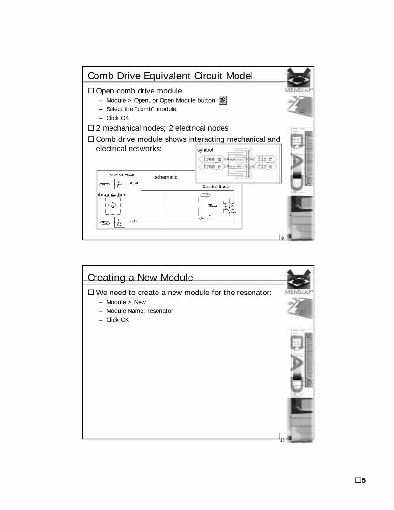
Creating a New Module¨We need to create a new module for the resonator:

– Module > New– Module Name: resonator– Click OK

¨6

11

Instancing a Module¨ To place a copy of another module in the current

module– Goto Module > Instance– Select the module to be instance from the list and click OK

• Instance will be inserted in the center of work area

– Move the instance to desired location – Modify instance parameters

12

Instancing Plate and Comb Drive¨ To instance the plate module

– Goto Module > Instance– Select “plate” in the Instance Module dialogue box and click OK– Use default location and parameters

¨ Similarly, instance the comb drive module– Goto Module > Instance– Select “comb” in the Instance Module dialogue box and click OK

¨ For the comb drive, we also need to move it

¨7

13

Selecting/Moving ¨ To select an object

– Click with the right mouse button, or– Select the Selection Tool , click with the left mouse button– Once selected:

• The selected object turns red• Its name will appear in the status bar

¨ To move an object– Select the object– Press the middle mouse button and drag the object to the

desired position– Move the comb drive instance to the right of the plate– Align the ports (represented by circles)

¨ To edit the parameters of an instance– Select the object– Goto Edit > Edit Object, or Ctrl + E

14

Duplicating Comb Drives ¨ To create a second instance of the comb drive:

– Select the first comb drive instance – Edit > Copy (Ctrl + C), then Edit > Paste (Ctrl + V)– Click on the left side of the place

¨ To change orientation of the left comb:– Select the left comb drive– Edit > Flip > Horizontal, or click the Flip Horiz. button

¨ Move the instances so that the connection ports are lined up

¨ You should have a schematic diagram that looks like this:

¨8

15

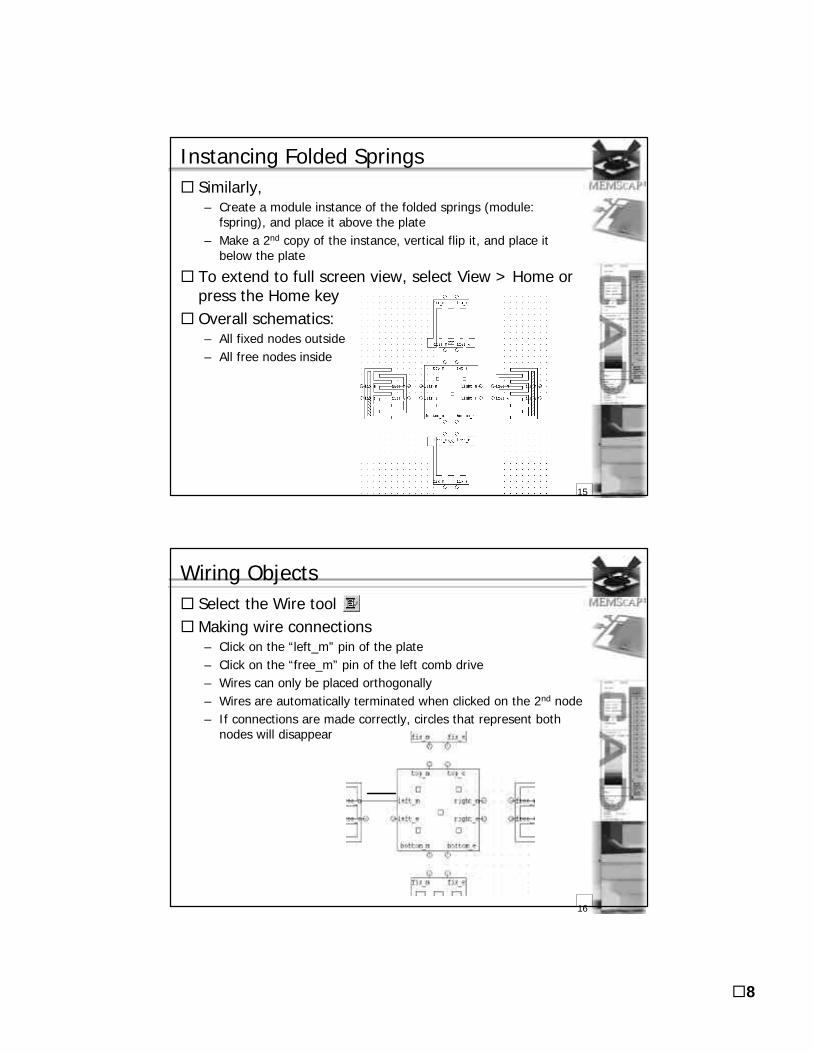
Instancing Folded Springs¨ Similarly,

– Create a module instance of the folded springs (module: fspring), and place it above the plate

– Make a 2nd copy of the instance, vertical flip it, and place it below the plate

¨ To extend to full screen view, select View > Home or press the Home key

¨ Overall schematics:– All fixed nodes outside– All free nodes inside

16

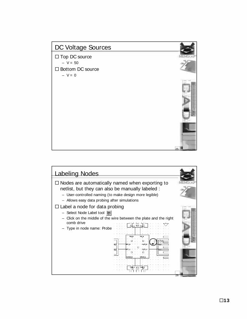
Wiring Objects¨ Select the Wire tool¨ Making wire connections

– Click on the “left_m” pin of the plate– Click on the “free_m” pin of the left comb drive– Wires can only be placed orthogonally– Wires are automatically terminated when clicked on the 2nd node– If connections are made correctly, circles that represent both

nodes will disappear

¨9

17

Complete Resonator Wiring¨ Connect the rest of the nodes between the springs,

comb drives, and plate:

18

Boundary Conditions¨ Mechanical boundary conditions:

– 5 Springs fix_m: fixed; displacement = 0– 5 Comb fix_m: fixed; displacement = 0

¨ Electrical boundary conditions:– 5 Spring fix_e: voltage = 50 V

• Connects to comb free_e through plate– 5 R comb fix_e: voltage = 0 V– 5 L comb fix_e: voltage = variable

¨ Now we will create the boundary conditions for the simulation:– Since displacement is mapped to voltage, both voltage and

displacement BC’s are created as voltage sources

¨10

19

Setting Boundary Conditions¨ Instancing AC voltage sources (Source_v_ac)

– Place it the left side of the left comb drive

¨ Instancing DC voltage sources (Source_v_ac)– Place it to the right side of the right comb drive

¨ Copy the instance of Source_v_dc and place it to the right of the top spring– Select the instance, Edit > Copy, Edit > Paste

20

Global Nodes¨ All the instances of a global module are connected to

each other regardless of whether they are connected by wires– Useful for frequently used nodes like power and ground

¨ To instance a global ground module – Click on the Global Symbol Instance button– Click on the bottom node of the AC source– Select the Gnd module

¨ Grounded AC source:

¨11

21

Global Nodes¨ Copy the Gnd instance to the other 2 voltage sources,

as well as 3 more instances next to the sources, and place them as follows:

22

Complete Schematic View¨ Use the Wire tool and connect the voltage sources

and ground to the module instances as follows:– All fix_m nodes to ground– All fix_e nodes to their respective voltage sources

¨12

23

Instance Properties¨ Module instances have properties that can be modified

– Properties are analogous to program variables and are used to store parametric description of modules

– Can store geometric (length, width, etc.) or behavioral (resistivity, etc.) parameters

¨ A property consists of name and value– Name: text– Value: can be text, number and tokens

¨ These properties are exported to the netlist

24

Changing Instance Properties¨ To change the AC voltage source

– Use the select tool to select the AC voltage source

– Click Edit > Edit Object, or Ctrl + E

¨ Change the following parameters:– 1 for mag– 0 for phase– 0 for Vdc

¨13

25

DC Voltage Sources¨ Top DC source

– V = 50

¨ Bottom DC source– V = 0

26

Labeling Nodes¨ Nodes are automatically named when exporting to

netlist, but they can also be manually labeled :– User-controlled naming (to make design more legible)– Allows easy data probing after simulations

¨ Label a node for data probing– Select Node Label tool– Click on the middle of the wire between the plate and the right

comb drive– Type in node name: Probe

¨14

27

Command Tool ¨ The Command Tool provides an interface for inserting

T-Spice simulation commands into your schematics– Pressing the Command Tool button – Click where the command is to be inserted in the work area– Enter information in pop-up window

28

Command Categories¨ Click the +/- sign to expand/collapse each category¨ After the category & subcategory are chosen, the right

side of the window allows the user to fill in options and parameters for the command

¨ For this tutorial, we will insert 2 simulation commands– Include foundry-dependent process data – Simulation parameters

¨15

29

Including Foundry Data¨ To insert the foundry data:

– Select Files > Include– Browse to the MUMPS process data file: Process_MUMPS.sp– Click Insert Command

¨ The inserted command should look something like this:

30

Foundry Data¨ Open MUMPS process file:

– Open C:\demo directory– Double click to open Process_MUMPS.sp

¨ This file contains information such as film thicknesses, material properties, and constants

¨16

31

Simulation Parameters¨ For this tutorial, we would like to perform an AC

analysis to study the frequency-dependent behavior of the resonator– With the Command Tool selected– Click below the last command created– Select Analysis > AC

• Frequency sample type: decade• Frequency per decade: 500• Frequency range: 10k to 100k• Sweep: Not used

– Click Insert Command

¨ The inserted command:

32

Final Schematic View

¨17

33

Setup Probing Parameters¨We need to set up where the simulation data will be

stored:– Goto Setup > Probing– For probing data file location, browse to your current working

directory (c:\demo), and type in Resonator.dat– Click OK

34

Generating Spice Netlist¨ Finally, to generate the Spice netlist of the current

schematics, press the T-Spice button¨ The T-Spice window displays the generated netlist

– Netlist: textual representation of the schematics

Simulation toolbar

Display/editor area

Output window

¨18

35

Starting Simulations¨ The simulation toolbar can be used to start, stop, and

pause a simulation¨ To start simulations, press the Start button¨ In the Run Simulation window

– Change Waveform options to: do not show– Click Start Simulation

36

Simulation Output¨ During simulation, a text window will display relevant

information during the simulation

¨ The bottom output window displays the status of the simulation:

¨19

37

Simulation Results¨ To view the results of the simulation, return to S-Edit.

– Select the Probe tool– Click on the Probe node we created

38

Waveform Display¨ The waveform viewer (W-Edit) opens and displays the

simulation results at the probed node.

Click the expand charts button

¨20

39

Simulation Results¨ Magnitude and phase plots separate into 2 charts

– Shows resonant frequency at ~13 kHz

¨ Chart display properties (axis, labels, scale, color, etc.) can be change from Chart > Options