System Identification of General Aviation Aircraft Using ...
123
System Identification of General Aviation Aircraft Using The Filter Error Technique Except where reference is made to the work of others, the work described in this thesis is my own or was done in collaboration with my advisory committee. This thesis does not include proprietary or classified information. Dakshesh Patel Certificate of Approval: John E. Cochran, Jr. Professor Aerospace Engineering Gilbert L. Crouse, Chair Associate Professor Aerospace Engineering David A. Cicci Professor Aerospace Engineering Joe F. Pittman Interim Dean Graduate School
Transcript of System Identification of General Aviation Aircraft Using ...
System Identification of General Aviation Aircraft
Using The Filter Error Technique
Except where reference is made to the work of others, the work described in this thesis ismy own or was done in collaboration with my advisory committee. This thesis does not
include proprietary or classified information.
Dakshesh Patel
Certificate of Approval:
John E. Cochran, Jr.ProfessorAerospace Engineering
Gilbert L. Crouse, ChairAssociate ProfessorAerospace Engineering
David A. CicciProfessorAerospace Engineering
Joe F. PittmanInterim DeanGraduate School

System Identification of General Aviation Aircraft
Using The Filter Error Technique
Dakshesh Patel
A Thesis
Submitted to
the Graduate Faculty of
Auburn University
in Partial Fulfillment of the
Requirements for the
Degree of
Master of Science
Auburn, AlabamaDecember 17, 2007
System Identification of General Aviation Aircraft
Using The Filter Error Technique
Dakshesh Patel
Permission is granted to Auburn University to make copies of this thesis at itsdiscretion, upon the request of individuals or institutions and at
their expense. The author reserves all publication rights.
Signature of Author
Date of Graduation
iii
Vita
Dakshesh Patel was born to Mahesh and Geeta, on March 15, 1983 in Ahmedabad.
He attended Nirma Institute of Technology, Ahmedabad and graduated in July 2004 with
Bachelor of Engineering in Instrumentation and Control. He joined Aerospace Engineering
Program at Auburn University as a Masters student in August 2004.
iv
Thesis Abstract
System Identification of General Aviation Aircraft
Using The Filter Error Technique
Dakshesh Patel
Master of Science, December 17, 2007(B.E., Nirma Institute of Technology, Gujarat University, 2004)
123 Typed Pages
Directed by Gilbert L. Crouse
An overview of some past and modern applications of system identification techniques
to aircraft is presented in this thesis, which traces progress and accomplishments in the
field of system identification - especially application to aircraft. The thesis also includes
the definition, meaning, importance, applications and necessity of the same. The funda-
mental parts of system identification, including model postulation, experimental design,
data analysis, parameter estimation, and model validation are explained. The filter error
technique of data analysis is detailed, for both linear and nonlinear systems. Techniques to
predict aircraft stability and control derivatives theoretically and analytically are explained
in some details. Two successfully investigated experiments of system identification using
flight data with results and comparison of the estimated parameters with published data
are demonstrated with details. The thesis is completed by some remarks made on possible
future advancement and concluding notes.
v
Acknowledgments
The author would like to thank his research advisor, Dr. Gilbert L. Crouse, for render-
ing constant guidance and motivation throughout his research. He also thanks Dr. Crouse
for showing complete trust in his abilities and providing him with an opportunity to con-
duct research in the exciting field of system identification. Dr. Crouse is a great mentor
and working with him was a wonderful and memorable experience for Dakshesh. The au-
thor would like to express his gratitude to Dr. John E. Cochran for teaching the courses
which greatly helped him in understanding the research problem and also for being part
of his graduate committee. He would like to thank Dr. David A. Cicci, for teaching the
fundamentals of estimation theory through orbit determination class and also for serving
as a graduate committee member.
The author is thankful to Ran Dai and Daroe Lee, for their friendship and help in
understanding the dynamics and control subjects. He would like to acknowledge his friends
at Auburn, with whom he spent memorable years. Particularly Palak, Vinita and Dhrumil’s
support and encouragement have always made his stay at Auburn, pleasant and enthusiastic.
The author wishes to dedicate this work to his parents and teachers for their enduring
love, immense moral support and encouragement in the journey of life.
vi

Style manual or journal used AIAA Journal of Aircraft
Computer software used LATEX and the departmental style-file “aums.sty”
vii
Table of Contents
List of Figures x
List of Tables xii
Nomenclature xiii
1 Introduction 11.1 System Identification - A Definition . . . . . . . . . . . . . . . . . . . . . . 1
1.1.1 Significance and Necessity of System Identification . . . . . . . . . . 21.1.2 Objectives of Research . . . . . . . . . . . . . . . . . . . . . . . . . . 4
1.2 Problem Description . . . . . . . . . . . . . . . . . . . . . . . . . . . . . . . 51.3 Progress of Aircraft System identification . . . . . . . . . . . . . . . . . . . 7
1.3.1 System Identification in General . . . . . . . . . . . . . . . . . . . . 71.3.2 System Identification of Aircraft . . . . . . . . . . . . . . . . . . . . 81.3.3 Deterministic and Non-Deterministic Analysis . . . . . . . . . . . . . 101.3.4 Latest Techniques of System Identification . . . . . . . . . . . . . . . 13
2 Background and Theoretical Development 162.1 Dynamical Model Description . . . . . . . . . . . . . . . . . . . . . . . . . . 162.2 Cost Function (Performance Index) J . . . . . . . . . . . . . . . . . . . . . . 172.3 Essentials of Cost Function Minimization . . . . . . . . . . . . . . . . . . . 172.4 Modified Newton-Raphson Algorithm . . . . . . . . . . . . . . . . . . . . . 20
3 System Identification of General Aviation Aircraft 233.1 Filter Error Technique for Linear Systems . . . . . . . . . . . . . . . . . . . 23
3.1.1 Kalman Filter . . . . . . . . . . . . . . . . . . . . . . . . . . . . . . . 253.1.2 Solution of Riccati Equation . . . . . . . . . . . . . . . . . . . . . . 263.1.3 Formulations for Process Noise . . . . . . . . . . . . . . . . . . . . . 283.1.4 The Filter Error Algorithm for Linear Systems . . . . . . . . . . . . 303.1.5 Parameter Update . . . . . . . . . . . . . . . . . . . . . . . . . . . . 32
3.2 Filter Error Technique for Non-linear Systems . . . . . . . . . . . . . . . . . 363.2.1 Steady State Filter . . . . . . . . . . . . . . . . . . . . . . . . . . . . 383.2.2 Parameter Update . . . . . . . . . . . . . . . . . . . . . . . . . . . . 41
viii
4 Prediction of Aircraft Stability and Control Derivatives 424.1 Steady State Coefficients . . . . . . . . . . . . . . . . . . . . . . . . . . . . . 434.2 Stability Derivatives . . . . . . . . . . . . . . . . . . . . . . . . . . . . . . . 45
4.2.1 Aircraft Speed Derivatives . . . . . . . . . . . . . . . . . . . . . . . . 464.2.2 Angle of Attack Derivatives . . . . . . . . . . . . . . . . . . . . . . . 474.2.3 Angle of Sideslip Derivatives . . . . . . . . . . . . . . . . . . . . . . 484.2.4 Roll Rate Derivatives . . . . . . . . . . . . . . . . . . . . . . . . . . 514.2.5 Pitch Rate Derivatives . . . . . . . . . . . . . . . . . . . . . . . . . . 534.2.6 Yaw Rate Derivatives . . . . . . . . . . . . . . . . . . . . . . . . . . 53
4.3 Control Derivatives . . . . . . . . . . . . . . . . . . . . . . . . . . . . . . . . 554.3.1 Aileron Control Derivatives . . . . . . . . . . . . . . . . . . . . . . . 564.3.2 Elevator Control Derivatives . . . . . . . . . . . . . . . . . . . . . . 574.3.3 Rudder Control Derivatives . . . . . . . . . . . . . . . . . . . . . . . 57
5 Investigated Examples of System Identification Using Flight Test Data 595.1 Estimation of Lateral Motion Derivatives using the Simulated Flight Data . 59
5.1.1 Comparison of the Results with the Original Experiment . . . . . . 615.1.2 Responses and Results . . . . . . . . . . . . . . . . . . . . . . . . . . 63
5.2 Estimation of Longitudinal Motion Derivatives of HFB-320 Aircraft . . . . 675.2.1 Comparison of the Results with the Original Experiment . . . . . . 705.2.2 Responses and Results . . . . . . . . . . . . . . . . . . . . . . . . . . 70
5.3 System Identification Applied to Model Aircraft Trainer . . . . . . . . . . . 735.3.1 The Investigated Aircraft Trainer - Hanger 9 Extra Easy . . . . . . 735.3.2 Responses and Results . . . . . . . . . . . . . . . . . . . . . . . . . . 74
5.4 Model Validation . . . . . . . . . . . . . . . . . . . . . . . . . . . . . . . . . 87
6 Summary 886.1 Concluding Notes . . . . . . . . . . . . . . . . . . . . . . . . . . . . . . . . . 886.2 Expected Future Applications of System Identification to Aircraft . . . . . . 89
Bibliography 91
A Discretization of continuous-time state equation 99A.1 Need of Discretization . . . . . . . . . . . . . . . . . . . . . . . . . . . . . . 99A.2 Determine Θ and Λ . . . . . . . . . . . . . . . . . . . . . . . . . . . . . . . . 100
B Numerical Integration using Runge-Kutta method, Order 4 102
ix
List of Figures
1.1 Block Diagram for System Identification to aircraft [1] . . . . . . . . . . . . 14
3.1 Block Diagram for Filter Error Technique [68] . . . . . . . . . . . . . . . . . 24
3.2 Algorithm of Filter Error Technique for Linear Systems [1] . . . . . . . . . . 31
3.3 Algorithm of Filter Error Technique for Nonlinear Systems [1] . . . . . . . . 37
4.1 Determination of Drag Coefficient from a known Lift Coefficient . . . . . . 44
5.1 The DLR de Havilland DHC − II Research Aircraft [84] . . . . . . . . . . 60
5.2 Comparison of Estimated(green) and Measured(blue) Responses for the Lat-eral Directional Motion of Aircraft . . . . . . . . . . . . . . . . . . . . . . . 64
5.3 Convergence Plots of Dimensional Derivatives for Lateral Directional Motionof Aircraft . . . . . . . . . . . . . . . . . . . . . . . . . . . . . . . . . . . . . 65
5.4 Cost Function Reduction for Lateral Directional Motion of Aircraft . . . . . 66
5.5 The DLR HFB − 320 Research Aircraft [87] . . . . . . . . . . . . . . . . . 67
5.6 Comparison of Estimated(green) and Measured(blue) Responses for the Lon-gitudinal Directional Motion of Aircraft . . . . . . . . . . . . . . . . . . . . 71
5.7 Convergence Plots of Non-Dimensional Derivatives for Longitudinal Direc-tional Motion of Aircraft . . . . . . . . . . . . . . . . . . . . . . . . . . . . . 72
5.8 Inputs for Longitudinal Motion . . . . . . . . . . . . . . . . . . . . . . . . . 72
5.9 Cost Function Reduction for Longitudinal Motion . . . . . . . . . . . . . . 73
5.10 Aircraft Trainer - Hanger 9 Extra Easy [91] . . . . . . . . . . . . . . . . . . 74
5.11 Comparison of Estimated(green) and Measured(blue) Responses for the Lat-eral Directional Motion of Aircraft . . . . . . . . . . . . . . . . . . . . . . . 77
x
5.12 Convergence Plots of Dimensional Derivatives for Lateral Directional Motionof Aircraft . . . . . . . . . . . . . . . . . . . . . . . . . . . . . . . . . . . . . 78
5.13 Cost Function Reduction for Lateral Directional Motion of Aircraft . . . . . 79
5.14 Comparison of Estimated(green) and Measured(blue) Responses for the Lat-eral Directional Motion of Aircraft . . . . . . . . . . . . . . . . . . . . . . . 80
5.15 Convergence Plots of Dimensional Derivatives for Lateral Directional Motionof Aircraft . . . . . . . . . . . . . . . . . . . . . . . . . . . . . . . . . . . . . 81
5.16 Cost Function Reduction for Lateral Directional Motion of Aircraft . . . . . 82
5.17 Comparison of Estimated(green) and Measured(blue) Responses for the Lon-gitudinal Directional Motion of Aircraft . . . . . . . . . . . . . . . . . . . . 84
5.18 Convergence Plots of Non-Dimensional Derivatives for Longitudinal Direc-tional Motion of Aircraft . . . . . . . . . . . . . . . . . . . . . . . . . . . . . 85
5.19 Input for Longitudinal Motion . . . . . . . . . . . . . . . . . . . . . . . . . 86
5.20 Cost Function Reduction for Longitudinal Motion . . . . . . . . . . . . . . 86
xi

List of Tables
5.1 Estimated dimensional derivatives of lateral motion of aircraft . . . . . . . . 62
5.2 Estimated non-dimensional derivatives of longitudinal motion of aircraft . . 69
5.3 Aerodynamic, geometric and mass data for the aircraft trainer . . . . . . . 75
5.4 Comparison between the predicted values and the estimated values of thedimensional derivatives for the lateral motion of the aircraft trainer . . . . . 76
5.5 Comparison between the predicted values and the estimated values of thedimensional derivatives for the lateral motion of the aircraft trainer . . . . . 82
5.6 Comparison between the predicted values and the estimated values of thenon-dimensional derivatives for the longitudinal motion of aircraft trainer . 83
xii

Nomenclature
1. English Symbols
a.c. aerodynamic center
A state matrix of a linear system, size n×n
Ah = bh2 / Sh horizontal tail aspect ratio
Av = bv2 / Sv vertical tail aspect ratio
Aw = b2 / S wing aspect ratio
ax, ay, az accelerations along x, y, z body axes, ft/s2
b wing span
bh horizontal tail span
bv vertical tail span
bx, by bias parameters of state and observation equations
c chord, ft
c mean geometric chord, ft
cr root chord, ft
ct tip chord, ft
c.g. aircraft center of gravity
C observation matrix, size m×n
CD aircraft drag coefficient
CD0 zero-lift drag coefficient
xiii

Cl aerodynamic rolling moment coefficient
CL aircraft lift coefficient
CL0 lift coefficient at zero angle of attack
Cm aerodynamic pitching moment coefficient
Cn aerodynamic yawing moment coefficient
CX coefficient of longitudinal force
CY coefficient of lateral(side) force
CZ coefficient of vertical force
D Drag
e span efficiency factor
ej jth unit vector
F state noise matrix, size n×n
also: aerodynamic force, N
FG magnitude of force due to gravity, N
FT magnitude of force due to thrust, N
Fe net thrust magnitude, N
f [·] vector of system state functions
G measurement noise matrix, size m×m
also: moment, Nm
g acceleration due to gravity, ft/s2
g[·] system observation function
xiv
I inertia matrix
Ixx rolling moment of inertia in body axes, slug-ft2
Ixz XZ product of inertia in body axes, slug-ft2
Iyy pitching moment of inertia in body axes, slug-ft2
Izz yawing moment of inertia in body axes, slug-ft2
J cost function
K filter-gain matrix, size n×m
k discrete-time index
lf fuselage length
lp horizontal distance between vertical tail a.c. and aircraft wing a.c.
lv horizontal distance between vertical tail a.c. and aircraft c.g.
L lift
m aircraft mass, lb
also: number of observation variables
m.g.c. mean geometric chord, ft
M free stream mach number
N number of data points
n number of state variables
P covariance matrix of the state error, size n×n
p, q, r roll, pitch, and yaw rates, rad/s
p, q, r roll, pitch, and yaw accelerations, rad/s2
xv

q dynamic pressure, N/ft2
rk kth diagonal element of R
R covariance matrix of residuals (innovations), size m×m
RN reynold’s number
S wing area, ft2
Sbfuse fuselage base area, ft2
Sfuse maximum fuselage cross section area, ft2
Sh horizontal tail area, ft2
Splf aircraft planform area, ft2
Sv vertical tail area, ft2
Swet total wetted area of aircraft, ft2
s number of input variables
t time, s
t/c thickness ratio at c
u control input vector, size s×1
u, v, w velocity components along x, y, and z body axes, ft/s
v measurement noise vector, size m×1
V airspeed, ft/s
V h horizontal tail volume coefficient
w state noise vector, size n×1
W aircraft weight, lb
xvi

x state vector, size n×1
Xac longitudinal position of a.c. on wing m.g.c., ft
Xach longitudinal position of horizontal tail a.c. on wing m.g.c., ft
Xw longitudinal distance from wing quarter chord m.g.c. to c.g., ft
y observation vector, size m×1
z measurement vector, size m×1
zf vertical height of fuselage at wing root chord, ft
zp vertical distance between vertical tail a.c. and aircraft wing a.c., ft
zv vertical distance between vertical tail a.c. and aircraft c.g., ft
zw wing distance to fuselage centerline, ft
2. Stability and Control Derivatives
CDV non-dimensional derivative of drag with respect to speed
CLV non-dimensional derivative of lift with respect to speed
CmV non-dimensional derivative of pitching moment with respect to speed
CDα non-dimensional derivative of drag with respect to angle of attack
CLα non-dimensional derivative of lift with respect to angle of attack
Cmα non-dimensional derivative of pitching moment with respect to angle of attack
Cmq derivative of pitching moment with respect to pitch rate
Cmδe derivative of pitching moment with respect to elevator deflection
Lp derivative of rolling moment with respect to roll rate
xvii
Lr derivative of rolling moment with respect to yaw rate
Lδa derivative of rolling moment with respect to aileron deflection
Lδr derivative of rolling moment with respect to rudder deflection
Lv derivative of rolling moment with respect to lateral(side) velocity
Lβ derivative of rolling moment with respect to sideslip angle
Np derivative of yawing moment with respect to roll rate
Nr derivative of yawing moment with respect to yaw rate
Nδa derivative of yawing moment with respect to aileron deflection
Nδr derivative of yawing moment with respect to rudder deflection
Nv derivative of yawing moment with respect to lateral(side) velocity
Nβ derivative of yawing moment with respect to sideslip angle
Yp derivative of side-force with respect to roll rate
Yr derivative of side-force with respect to yaw rate
Yδa derivative of side-force with respect to aileron deflection
Yδr derivative of side-force with respect to rudder deflection
Yv derivative of side-force with respect to lateral(side) velocity
Yβ derivative of side-force with respect to sideslip angle
3. Greek Symbols
α angle of attack, deg
β sideslip angle, deg
xviii

also: (1−M2)1/2
γ flight path angle, deg
Γ dihedral, deg
δa, δe, δr aileron, elevator, and rudder deflections, deg
δx perturbation in x
δΘ perturbation in Θ
∆t sampling time, s
∆Θ vector of parameter update
ε downwash angle at the horizontal tail, deg
εt wing twist angle, deg
η span fraction
ηh ratio of horizontal tail to wing dynamic pressure
λ = ct/cr taper tatio
Λc/2 semi-chord sweep angle, deg
Λc/4 quarter-chord sweep angle, deg
ΛLE leading edge sweep angle, deg
µ coefficient of viscosity for air
ω angular velocity, rad/s
Φ vector of unknown parameters
ρ density of air, lb/ft3
σ side-wash angle, deg
xix

σT tilt angle of the engines, deg
θ pitch angle, deg
Θ state transition matrix
ϑ vector of process noise distribution matrix, F
ζ vector of system parameters
4. Superscripts
T transpose
−1 inverse
∼ predicted estimates
∧ corrected estimates
5. Subscripts
a aileron
b base
cg center of gravity
cs cross sectional
e elevator
fus fusalage
h horizontal tail
i, j general indices
xx

k discrete-time index
LE leading edge
m measured variables
max maximum
M (at a given) mach number
p perturbed variables
plf planform
r rudder
ref reference, usually the wing, or a point on the wing
v vertical tail
w wing
wet wetted
0 initial condition
xxi

Chapter 1
Introduction
The thesis describes the system identification technique and its applications related
only to aircraft, but the system identification has been successfully applied to many diverse
fields. The system identification is basically related to modeling from experimental data and
can be applied to many different fields such as: economics, biology, materials, engineering,
automobiles, medicine and aerospace engineering.
1.1 System Identification - A Definition
System identification is a discipline of science which attempts to answer the inverse
problem. It tries to characterize a system in a suitable form based on observations of
the system’s behavior. The process of system identification involves certain fundamental
assumptions [1]:
1. The true state of the dynamic system is deterministic.
2. Physical principles underlying the dynamic process can be modeled.
3. It is possible to carry out specific experiments.
4. Measurements of system inputs and outputs are available.
In the year 1962, Zadeh [2] gave a technical definition for system identification as: “System
identification is the determination, on the basis of observation of input and output, of a
1

system within a specified class of systems to which the system under test is equivalent.”
Several important features of system identification are highlighted by this description: the
necessity of obtaining input and output data, model characterization and selecting the best
model from the selected class. Iliff [3] provided a philosophical definition in contrast with
the above technical definition as: “Given the answer, what are the questions, that is, look
at the results and try to figure out what situation caused those results.” This definition
points out the prime approach behind the model building process, namely that system
identification is an inverse problem.
1.1.1 Significance and Necessity of System Identification
The system identification tries to determine the best parameters for an assumed math-
ematical model, which is made up of differential equations. The unknown parameters are
determined indirectly from measured data. Considering the aircraft system identification
problem, assume Φ is an unknown parameter vector, which contains unknown stability and
control parameters of the dynamics equations, which are to be estimated. As a first part
of system identification, a parameter estimation technique is used to estimate the unknown
parameter vector Φ, such that the system response y fits the measured system response
z adequately. In aircraft system identification the measured system response is typically
flight test data. After the parameter estimation is performed, a second and more important
part, known as model validation needs to follow. It evaluates model reliability. If it seems
that the identified model does not agree with the specific system standards and also the
2
statistical properties of the estimated parameters do not agree with the standards, then the
postulated model structure needs to be changed. Generally both steps must be repeated
again and again until the model is validated.
If the experimental model is already validated, then only the first part, parameter
estimation, is dealt with. If the model structure is not known and adequate information
about the system structure is not available, the system identification technique is dealt with
as a whole, which includes both parameter estimation and model validation.
After mentioning the definition, meaning and significance of system identification and
parameter estimation, the next question is, what is the necessity of system identification.
Why and where is system identification needed? This question must be answered due to
the two following examples of questions that have been raised about the utility of system
identification.
1. During one of the early American Institute of Aeronautics and Astronautics (AIAA)
conferences, someone raised a question: “When the aircraft is past the design and pro-
duction stage, and already flying, why and where do you need system identification?”[4]
2. An anonymous paper reviewers comment: “After perhaps 30 years of journal articles
and conferences on system identification, hardly any results have been of engineering
utility. Or if they are in use, the fact is not widely published.”[4]
In flight vehicle development, system identification is a necessary step because it leads to
adequately accurate and validated mathematical models of flight vehicles, which are required
to [1],
3
1. understand the cause-effect relationship that underlines a physical phenomenon,
2. investigate system performance and characteristics,
3. verify wind-tunnel and analytical predictions,
4. develop high-fidelity aerodynamic databases for flight simulators meeting FAA fidelity
requirements,
5. support flight envelope expansion during prototype testing,
6. derive high-fidelity and high-bandwidth models for in-flight simulators,
7. design flight control laws including stability augmentation systems,
8. reconstruct the flight path trajectory, including wind estimation and incidence anal-
ysis,
9. perform fault-diagnosis and adaptive control or reconfiguration, and
10. analyze handling qualities specification compliance.
Due to the advantages and the uses given above the system identification is made an essential
part of aerospace system design and development.
1.1.2 Objectives of Research
The aim of this thesis and research work, is to contribute to the field of system iden-
tification of aircraft which has advanced over the recent decades, concentrating specifically
4
on nonlinear systems and time domain methodologies. Efficient and effective system iden-
tification of aircraft is only possible if the applied approach is well coordinated and follows
specific research guidelines. The thesis uses the filter error approach for all three examples
and tries to accommodate full details of such an efficient approach, summarizing the gen-
eral important concepts, techniques, computational procedures and three selected examples,
which were investigated based on the method.
1.2 Problem Description
The objective of system identification is to estimate the values of some unknown pa-
rameters in the system equations, which best represent the actual aircraft response, given a
set of flight time histories of an aircraft’s response variables. Here, the unknown parameters
are stability and control parameters.
The typical mathematical approach to this problem is to minimize the difference be-
tween the flight response and the response computed from the system equations. This
difference can be defined for each response variable as the integral of the error squared.
Then the signal errors can be multiplied by weighting factors and summed to obtain the
response error which defines an integral squared error criterion.
A mathematically more precise formulation can be made in probabilistic terms. A
probability that the estimated aircraft response time histories take on the values actually
observed can be defined for each possible estimate of unknown parameters. These parameter
5

estimates should be chosen so that this probability is maximized. This is known as a
maximum likelihood formulation of the problem.
To describe the maximum likelihood estimator mathematically, it is necessary to define
the equations of motion for the aircraft system. The following steps should be followed.
1. Derive the dynamical equations of motion.
2. Predict the unknown stability and control parameters.
3. Define the control inputs.
4. Express integral squared error criterion (to find a vector of unknowns), which mini-
mizes the cost function (performance index) J.
5. Estimate the state error covariance matrix to construct the likelihood function.
6. Minimize the cost function. The modified Newton-Raphson method seems most suit-
able for aircraft derivative determination, both in terms of computer time and con-
vergence properties.
7. Include prior information. Information from wind tunnel tests, previous real-time
flight tests and simulated flight test results are often available with the values of
some of the aircraft derivatives. It may be desirable to include this information in
the algorithm. The use of this information is particularly important when there is a
linear dependence between the response and the unknown parameters.
6
1.3 Progress of Aircraft System identification
A brief survey of the various contributions to the system identification field is presented
in this section, starting with applications in many fields. Applications to aircraft will follow.
Finally, the most modern techniques are briefed.
1.3.1 System Identification in General
The evolution from older system identification methods to statistically more accurate
approaches has been gradual. References can be found going back to the 18th century,
when Gauss [5] and Bernoulli [6] approached the system identification problem. The oldest
reference was found in the year 1777, when Bernoulli arrived at a solution by differentiating
the likelihood function [6]. Bernoulli used the concepts of maximum likelihood and least-
squares solution, though he did not introduce these terms. In the year 1809, Gauss [5]
used the maximum likelihood principle. In the reference mentioned, he discussed the least-
squares method for orbit determination of the earth from astronomical measurements.
Following the fundamental methods of Bernoulli and Gauss during the 18th century,
the maximum likelihood estimator was first discussed by Fisher [7] in the year 1912, as a
general statistical parameter estimator. Douglas [8] discussed “Inverse Problem Theorems”
in 1940. Feldbaum [9] considered the identification and control of the system as a single
problem in the “dual-control” theory; which was a little different than others, but still his
work was one of the most significant and also aimed at the present direction of investigation.
7
Research work in system identification theory prior to 1970, has been briefed in outstanding
research survey papers [10-13].
There are two kinds of system identification problems: deterministic (without state
noise) and non-deterministic (with state noise). Until the early forties, work on system
identification focus on the deterministic problem. But, succeeding the initial work in 1941-
1942 of Kolmogorov [14] and Wiener [15] the focus gradually shifted from deterministic
estimation to stochastic estimation. It was in the year 1960, when Kalman [16] followed basic
theories of Wiener and formulated a recursive solution to a filtering problem. This recursive
solution was directly executable through digital computations. Therefore, the Kalman filter
became popular quickly. Today it is the most widely used method for stochastic estimation.
The first experimentation of the maximum likelihood estimator on a digital computer and
application to parameters estimation in an industrial plant was done by Astrom and Bohlin
in 1965 [17]. This was the beginning of the modern era of system identification methods.
1.3.2 System Identification of Aircraft
The aerodynamic modeling, which obtains relationships between the three forces X,
Y and Z along the three cartesian coordinates, and the moments L, M and N about these
axes as functions of linear translational motion variables u, v, w and rotational rates p, q,
r was introduced in the early 20th century [18, 19]. This was the initiation of the evolution
of aircraft system identification. After the pioneering work of Bryan [18], numerical, sta-
tistical and experimental research was started in the field of real-time dynamics stability
8

and control. Glauert [20] initiated analyzing the phugoid motion of an aircraft in 1919 and
Norton [21, 22] presented papers in 1923 on estimation of stability and control derivatives.
The developments over the last nine decades have led to three different, but complementary
techniques for determining aerodynamic coefficients: 1) analytical methods, 2) wind-tunnel
methods, and 3) flight test methods [19].
The analytical methods and the wind-tunnel methods are performed to generate basic
information about the aerodynamic flight coefficients. Research in the computational fluid
dynamics field in recent years has positively affected the analytical approaches by providing
numerical solutions of complete configurations via sophisticated and advanced Euler and
Navier-Stokes flow solvers [19, 23, 24]. Experimental methods are important to validate the
analytical estimations. Wind-tunnel techniques, have in the past provided a huge amount
of data on innumerable flight vehicle configurations and are, as a rule, a basis for any new
flight vehicle design [19]. These techniques are, however, often associated with certain lim-
itations of validity arising out of, for example, model scaling, Reynolds number, dynamic
derivatives, cross coupling, and aero servo elasticity effects [19]. Determination of aerody-
namic derivatives from flight measurements is, therefore, important and necessary to reduce
limitations and uncertainties of the aforementioned two methods [19] and [25].
While detailing the chronological survey of research which led to the development and
universal acceptance of the maximum-likelihood estimation technique for aircraft stability
and control derivatives estimation, the more straightforward deterministic analysis will be
discussed first, which will be followed by non-deterministic analysis. References [26] and [27]
9
discuss some of the investigations in estimation of unknown stability and control derivatives
of an aircraft from aircraft dynamic response data.
1.3.3 Deterministic and Non-Deterministic Analysis
1. Deterministic Analysis: System identification methods have become more ele-
gant and complex since Kalman’s contribution. The steady-state oscillator excitation
analysis by Breuhaus [28] and Milliken [29, 30] and also the pulse input method uti-
lizing Fourier analysis [31] are examples of the frequency response method, which
increased in popularity for aircraft analysis during the 1940s and 1950s. These meth-
ods produced the frequency response of the vehicle, but not the stability and control
derivatives of the differential equations. Greenberg [32] and Shinbrot [33] attempted
to extract those parameters by defining the values of the aircraft parameters that re-
sulted in the best fit of the frequency response. Weighted least-square [33] and linear
least-squares [34] techniques were also applied to flight data in the 1960s. But these
techniques give poor results in the presence of measurement noise and yield biased
estimates. Also, they are time consuming and singularities are a serious problem with
them. The response curve-fitting technique [35] was formulated in 1951, which is
equivalent to the output error technique. But due to the lack of efficient and faster
computational means it did not work at that time.
In the 1950s and 1960s, time-vector methods [36-40] were commonly applied graph-
ical procedures to determine aircraft parameters from flight data. However, those
10

methods give an incomplete set of parameters and only the responses of fairly simple
motion can be analyzed. In the early 1960s, before the invention of digital computers,
analog matching techniques [40, 41] which are time consuming and somewhat tedious,
were applied to flight data. Resulting estimates differed depending on the skill and
knowledge of the person. Discussion of these past techniques concluded that a more
complete method of identification was needed, which can be faster and gives better
results.
Two separate articles [42, 43] on output error methods for obtaining aerodynamic
coefficients were published in the 1968. Taylor, Lawrence and Iliff [42] discussed the
maximum-likelihood estimator for obtaining a complete set of aerodynamic parame-
ters from flight data. Larson and Fleck [43] described a quasi-linearization method for
parameter identification of an aircraft. This research had produced an excellent model
which sufficiently described the resulting motion of the aircraft; which is the reason
for the success of these two methods. Due to these two studies on aircraft identifi-
cation using nonlinear minimization techniques, the interest in analysis of flight data
was increased. After only a year in the 1969, Taylor and Iliff [44] modified these two
techniques to include prior information. Minimization of this modified cost function
does not result in a maximum-likelihood estimator because it was based on the joint
probability distribution rather than the conditional probability [45]. Some excellent
and very successful computer algorithms on system identification have been published
11
[46-50]. The maximum likelihood estimator method was found very useful for flight
dynamic response [47-55].
Mehra [51] applied the Kalman filter to estimate aircraft aerodynamic parameters,
which produced poor results, because the state estimation and parameter estimation
were both biased. Hence, they did not converge to good results. Taylor, Powell and
Mehra [56] obtained better results after addition of the derivative of the state. In
the Netherlands, two successful applications of the Kalman filter, providing the state
estimation and aircraft parameters identification were obtained [57, 58].
2. Non-Deterministic Analysis: There are two types of techniques applied for pa-
rameter estimation with measurement and state noise: the Kalman filter technique
[51, 56-62] and maximum-likelihood estimator technique [52, 53, 63-65]. In the case of
non-deterministic analysis, the maximum likelihood estimator technique is normally
known as the filter error method. It was after 1965 that Astrom [59] and Kashyap
[60] described general applications of the extended Kalman filter. During 1970, for
the discrete-time system Taylor, Powell and Mehra [56] applied the extended Kalman
filter to simulated aircraft data with a state noise input. Chen and Eulrich [61] ex-
perimented with an application to that of Taylor, Powell and Mehra in 1971, but
it produced inconclusive results, as the state noise input was small, and also due to
nonlinearity of the system. Yazawa [62] produced very good results, when he applied
a simplified extended Kalman filter.
12
Iliff [65] applied the maximum-likelihood technique to output data of an aircraft flying
in atmospheric turbulence. The results were similar for the same aircraft flying in
smooth air, which is without state noise.
1.3.4 Latest Techniques of System Identification
The maximum likelihood estimator technique is used in most of the latest techniques
of system identification. One of these methods, the filter error technique is completely
detailed in Chapter 3. The digital computers of the modern era have the speed to imple-
ment self-regulating and self-governing data processing capability, which has changed the
concentration of flight test data analysis utilizing methods based on frequency domain to
methods based on time domain. Using modern computers, relatively larger numbers of
aircraft stability and control derivatives can be estimated from only a single aircraft test.
A coordinated approach based on flight test instrumentation, flight test techniques, and
methods of data analysis gradually evolved for system identification as applied to aircraft
[19, 46]:
1. Instrumentation and filters, which cover the entire flight data acquisition process
including adequate instrumentation and airborne or ground-based digital recording
equipment. Effects of all kinds of data quality should be accounted.
2. Flight test techniques, which are related to the selected flight vehicle maneuvering
procedures. The input signals should be optimized in their spectral composition to
excite all response modes from which parameters are to be estimated.
13
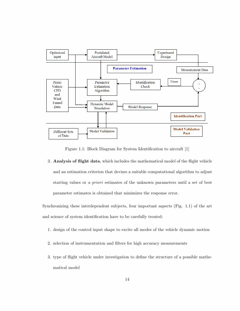
Figure 1.1: Block Diagram for System Identification to aircraft [1]
3. Analysis of flight data, which includes the mathematical model of the flight vehicle
and an estimation criterion that devises a suitable computational algorithm to adjust
starting values or a priori estimates of the unknown parameters until a set of best
parameter estimates is obtained that minimizes the response error.
Synchronizing these interdependent subjects, four important aspects (Fig. 1.1) of the art
and science of system identification have to be carefully treated:
1. design of the control input shape to excite all modes of the vehicle dynamic motion
2. selection of instrumentation and filters for high accuracy measurements
3. type of flight vehicle under investigation to define the structure of a possible mathe-
matical model
14
4. the quality of data analysis by selecting the most suitable time or frequency domain
identification method
The above four points must be followed carefully while investigating each aircraft. If they
are followed, modern system identification methods for aircraft can generally be expected
to provide good results. The modern techniques of data analysis for parameter estimation
are classified as: 1) Equation error technique, 2) Output error technique, 3) Filter error
technique. The last technique has been chosen for this study and is discussed in Chapter 3.
System identification is a multidisciplinary technique, which covers the fields of control
theory, numerical techniques, theories of statistics, sensors and instrumentation, flight test
techniques, signal processing, and flight dynamics. Basic knowledge of each of these fields
enables the user to generate efficient results.
15

Chapter 2
Background and Theoretical Development
Dynamical systems can generally be characterized by differential equations, whose or-
der is dependent on the complexity of the whole process. The system identification process
starts with postulating a model, so that it becomes possible to estimate the parameters of
state through simulation. Usually this is done by solving an initial value problem utilizing
numerical integration techniques. For system identification of aircraft, state space dynam-
ical models characterizing the aircraft motion are usually used. These models are derived
from Newtonian mechanics; which gives well formulated kinematic equations of aircraft
motion with translational and rotational degrees of freedom [66].
2.1 Dynamical Model Description
As stated earlier, the system identification process for aircraft starts with postulating
a dynamical model and governing equations of aircraft motion. The equations of motion
also include the output and measurement equations. The complete set of equations is then
[66]:
x=f [x(t),u(t),ζ]+F (ϑ)w(t), x(t0)=x0
y=g[x(t),u(t),ζ]
z(tk)=y(tk)+Gv(tk) (2.1)
16

where x is the (n×1) state vector, u is the (s×1) input vector, y is the (m×1) observation
vector and z is the (m×1) measurement vector. The unknown parameter vector Φ is given
as:
Φ=[ζT ϑT x0T ]T (2.2)
In this specific case of system identification to aircraft, the system parameter vector ζ is
made up of aircraft stability and control derivatives. The above nonlinear dynamical model
can be linearized if required, using numerical approximation.
2.2 Cost Function (Performance Index) J
Using the measurement vector z(t), observation vector y(t), measurement noise covari-
ance matrix R (m×m), for ny observation variables and N data points, a cost function, or
performance index, J can be defined as follows [67].
J(Φ, R) =12
∫ N
1[z(t)− y(t)]T R−1 [z(t)− y(t)] dt+
N
2ln [det(R)] +
Nny2
ln det(2π) (2.3)
where Φ is a column vector of parameters, which are to be estimated.
2.3 Essentials of Cost Function Minimization
For any experiment, the number of observations ny and number of data points N shall
be fixed. So, the last term in the above equation is a constant and hence can be neglected
17
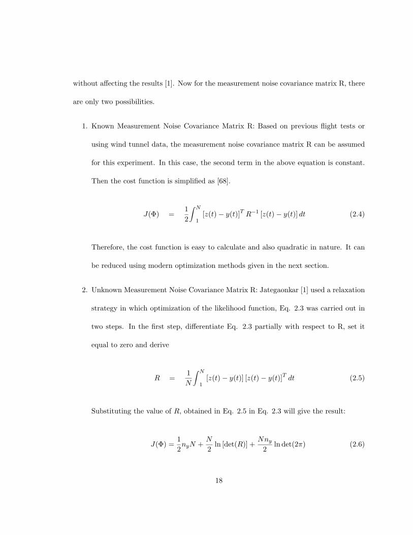
without affecting the results [1]. Now for the measurement noise covariance matrix R, there
are only two possibilities.
1. Known Measurement Noise Covariance Matrix R: Based on previous flight tests or
using wind tunnel data, the measurement noise covariance matrix R can be assumed
for this experiment. In this case, the second term in the above equation is constant.
Then the cost function is simplified as [68].
J(Φ) =12
∫ N
1[z(t)− y(t)]T R−1 [z(t)− y(t)] dt (2.4)
Therefore, the cost function is easy to calculate and also quadratic in nature. It can
be reduced using modern optimization methods given in the next section.
2. Unknown Measurement Noise Covariance Matrix R: Jategaonkar [1] used a relaxation
strategy in which optimization of the likelihood function, Eq. 2.3 was carried out in
two steps. In the first step, differentiate Eq. 2.3 partially with respect to R, set it
equal to zero and derive
R =1N
∫ N
1[z(t)− y(t)] [z(t)− y(t)]T dt (2.5)
Substituting the value of R, obtained in Eq. 2.5 in Eq. 2.3 will give the result:
J(Φ) =12nyN +
N
2ln [det(R)] +
Nny2
ln det(2π) (2.6)
18
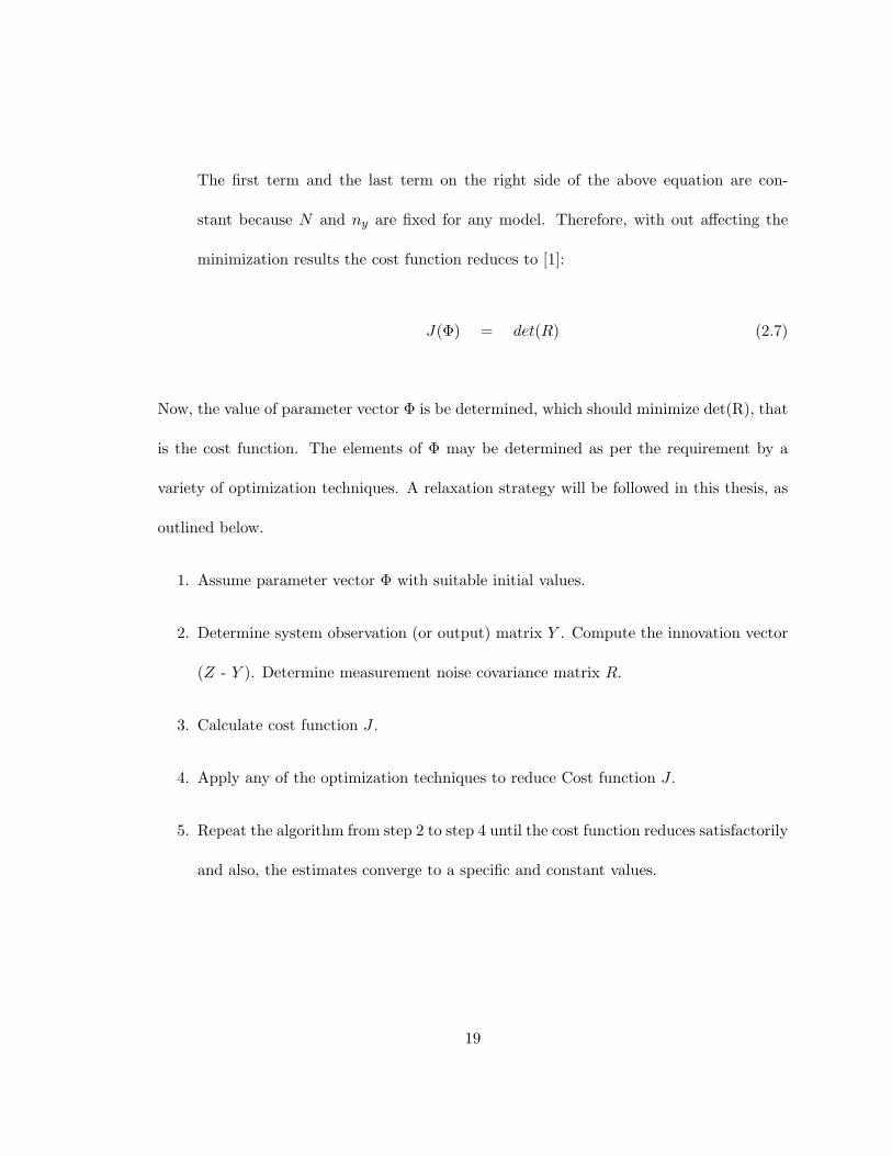
The first term and the last term on the right side of the above equation are con-
stant because N and ny are fixed for any model. Therefore, with out affecting the
minimization results the cost function reduces to [1]:
J(Φ) = det(R) (2.7)
Now, the value of parameter vector Φ is be determined, which should minimize det(R), that
is the cost function. The elements of Φ may be determined as per the requirement by a
variety of optimization techniques. A relaxation strategy will be followed in this thesis, as
outlined below.
1. Assume parameter vector Φ with suitable initial values.
2. Determine system observation (or output) matrix Y . Compute the innovation vector
(Z - Y ). Determine measurement noise covariance matrix R.
3. Calculate cost function J .
4. Apply any of the optimization techniques to reduce Cost function J .
5. Repeat the algorithm from step 2 to step 4 until the cost function reduces satisfactorily
and also, the estimates converge to a specific and constant values.
19
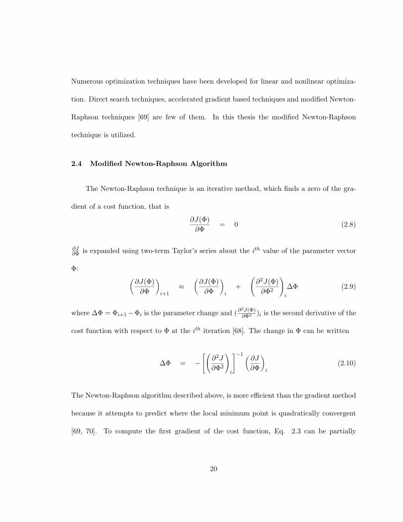
Numerous optimization techniques have been developed for linear and nonlinear optimiza-
tion. Direct search techniques, accelerated gradient based techniques and modified Newton-
Raphson techniques [69] are few of them. In this thesis the modified Newton-Raphson
technique is utilized.
2.4 Modified Newton-Raphson Algorithm
The Newton-Raphson technique is an iterative method, which finds a zero of the gra-
dient of a cost function, that is
∂J(Φ)∂Φ
= 0 (2.8)
∂J∂Φ is expanded using two-term Taylor’s series about the ith value of the parameter vector
Φ: (∂J(Φ)∂Φ
)i+1
≈(∂J(Φ)∂Φ
)i
+
(∂2J(Φ)∂Φ2
)i
∆Φ (2.9)
where ∆Φ = Φi+1−Φi is the parameter change and (∂2J(Φ)∂Φ2 )i is the second derivative of the
cost function with respect to Φ at the ith iteration [68]. The change in Φ can be written
∆Φ = −[(
∂2J
∂Φ2
)i
]−1 (∂J
∂Φ
)i
(2.10)
The Newton-Raphson algorithm described above, is more efficient than the gradient method
because it attempts to predict where the local minimum point is quadratically convergent
[69, 70]. To compute the first gradient of the cost function, Eq. 2.3 can be partially
20
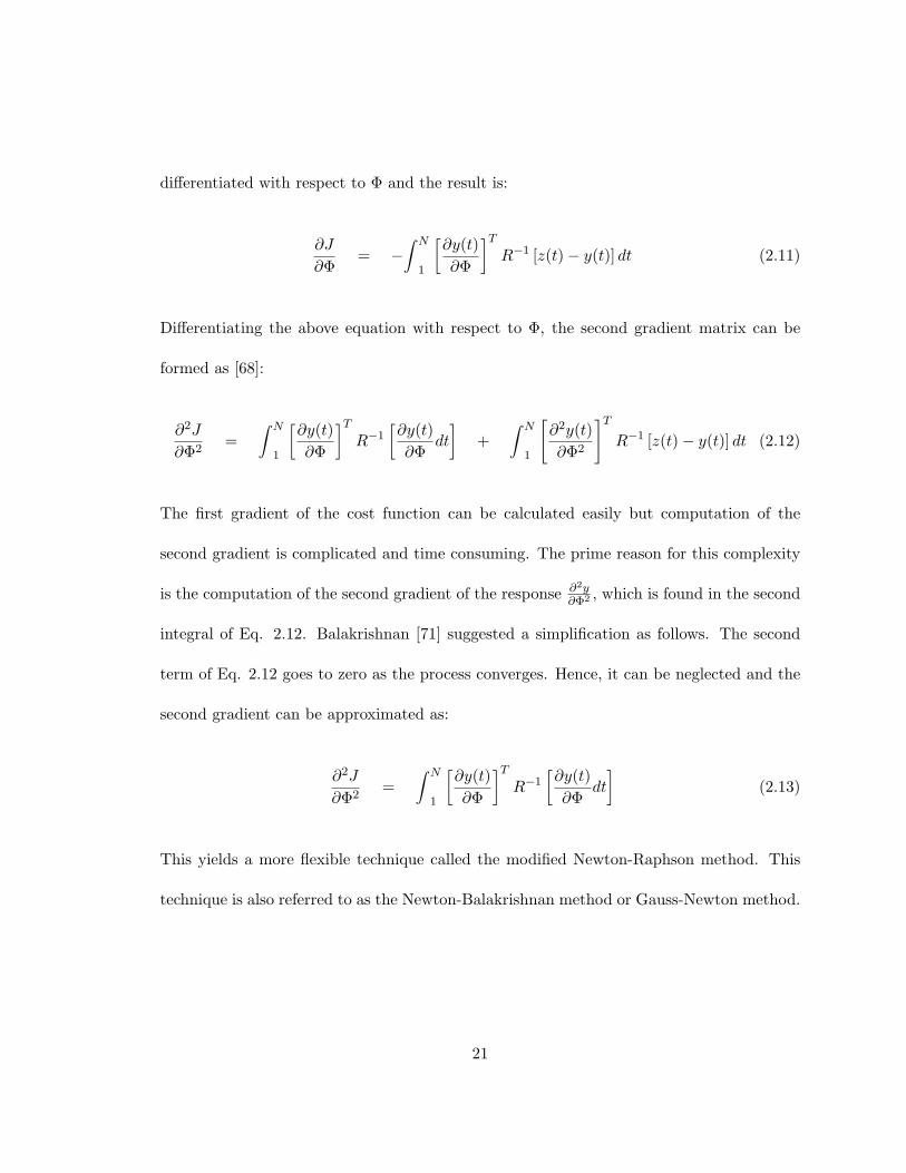
differentiated with respect to Φ and the result is:
∂J
∂Φ= −
∫ N
1
[∂y(t)∂Φ
]TR−1 [z(t)− y(t)] dt (2.11)
Differentiating the above equation with respect to Φ, the second gradient matrix can be
formed as [68]:
∂2J
∂Φ2=
∫ N
1
[∂y(t)∂Φ
]TR−1
[∂y(t)∂Φ
dt
]+
∫ N
1
[∂2y(t)∂Φ2
]TR−1 [z(t)− y(t)] dt (2.12)
The first gradient of the cost function can be calculated easily but computation of the
second gradient is complicated and time consuming. The prime reason for this complexity
is the computation of the second gradient of the response ∂2y∂Φ2 , which is found in the second
integral of Eq. 2.12. Balakrishnan [71] suggested a simplification as follows. The second
term of Eq. 2.12 goes to zero as the process converges. Hence, it can be neglected and the
second gradient can be approximated as:
∂2J
∂Φ2=
∫ N
1
[∂y(t)∂Φ
]TR−1
[∂y(t)∂Φ
dt
](2.13)
This yields a more flexible technique called the modified Newton-Raphson method. This
technique is also referred to as the Newton-Balakrishnan method or Gauss-Newton method.
21

This leads to a system of linear equations that can be summarized as follow [68]:
Denote P1 = −[(
∂2J
∂Φ2
)i
]−1
and P2 =(∂J
∂Φ
)i
(2.14)
From Eq. 2.11 and Eq. 2.13:
P1 =∫ N
1
[∂y(t)∂Φ
]TR−1
[∂y(t)∂Φ
dt
](2.15)
P2 = −∫ N
1
[∂y(t)∂Φ
]TR−1 [z(t)− y(t)] dt (2.16)
Then,
Φi+1 = Φi + ∆Φ, where ∆Φ = −P1−1P2 (2.17)
22

Chapter 3
System Identification of General Aviation Aircraft
The various aircraft parameter estimation techniques are:
1. The equation error technique
2. The output error technique
3. The filter error techniques
4. The frequency domain techniques
5. The recursive parameter estimation technique
6. The artificial neural network based techniques
A filter error technique is used in this thesis. The filter error techniques represent the general
stochastic approach to aircraft system identification introduced by Balakrishnan [63]. Iliff
[65] and Mehra [51, 56, 72] utilized these techniques in the 1970s. These techniques are
highly efficient while working with measurement and process noise.
3.1 Filter Error Technique for Linear Systems
A block diagram of the filter error technique is shown in Fig. 3.1. In this section, the
filter error technique for linear systems will be discussed with theoretical advancements and
computational aspects.
23

Figure 3.1: Block Diagram for Filter Error Technique [68]
A dynamic system can be described by the following stochastic linear mathematical
model [1].
x(t) = Ax(t) +Bu(t) + Fw(t) + bx, x(t0) = 0 (3.1)
y(t) = Cx(t) +Du(t) + by (3.2)
z(tk) = y(tk) +Gvk, k = 1, 2, ...N (3.3)
where x is a state vector (n×1), u is a control input vector (s×1), y is an output vector
(m×1), and z is a measurement vector (m×1) sampled at N discrete time points. Matrices A
(n×n), and C (m×n), contain unknown stability derivatives and matrices B (n×s), and D
(m×s), contain unknown control derivatives. Matrices F (n×n), and G (m×m), represent
24

the process and measurement noise distribution matrices, respectively. In the state and
observation equations, bx and by are bias terms. In the most general case all of the elements
of the matrices A, B, C, D and bias terms, bx and by form the parameter vector Φ, which
is to be estimated.
From the Eqs. 2.3-2.4, output vector, y, is required now, to calculate the cost function
J and the measurement noise covariance matrix, R. A Kalman filter is used to estimate the
output vector given the observed data, Ztk . Parameter estimates for Φ and R are obtained
by minimizing the cost function.
Though it can be assumed that the process and measurement noises are additive, the
estimation process is still complicated because the nature of the system is non-deterministic
[67]. Because of the process and measurement noise, it is not possible to integrate the state
equations. Instead, a standard Kalman filter is utilized as an optimal state estimator for
the linear system [73, 74].
3.1.1 Kalman Filter
The Kalman filter consists of two steps, a prediction and a correction step.
1. Prediction step: For the linear model postulated in Eqs. 3.1-3.2, the prediction step
is given by [1]:
x(tk+1) = Θx(tk) + ΛBu(tk) + Λbx (3.4)
y(tk) = Cx(tk) +Du(tk) + bx (3.5)
25

2. Correction step
x(tk) = x(tk) +K[z(tk)− y(tk)] (3.6)
Here, x is a predicted state vector, x is a corrected state vector, u is an average of the
control input at two successive discrete time steps, y is a predicted observation vector and
[z(tk)− y(tk)] is the residual (or innovation). Θ and Λ are the state transition matrix and
integral of state transition matrix (derived in appendix A). K is the Kalman gain (n×m)
and is dependent on the observation matrix C, state prediction error covariance matrix P
(n×n), and measurement error covariance matrix R (m×m), and given as [67]:
K = PCTR−1 (3.7)
The measurement noise covariance matrix R can be found using Eq. 2.5 and the state
prediction error covariance matrix P is calculated by solving the Riccati equation.
3.1.2 Solution of Riccati Equation
The Riccati equation is solved to compute the state prediction error covariance matrix,
P . A steady-state form of the continuous-time Riccati equation is used here because it is
easier than the discrete-time equation [1, 67, 75]. The first order projection of the Riccati
equation is given below.
AP + PAT − 1∆t
PCTR−1CP + FF T = 0 (3.8)
26

Eq. 3.8 can be solved using Potter’s method [1, 76] based on eigenvector decomposition.
Only the necessary details are provided here. Solution of the Riccati equation follows three
steps and is very straightforward.
1. Start with formulation of the Hamiltonian matrix, H, as [67]:
H =
[A | − FF T
− 1∆tC
TR−1C | −AT
](3.9)
2. Compute the eigenvalues and eigenvector of the Hamiltonian matrix, H. Divide the
eigenvector matrix into four equal size matrices such that the eigenvectors related to
eigenvalues with positive real parts remain on the left side. Controllability due to
process noise and observability ensure that exactly one half of the eigenvectors will
have positive real parts (i.e., unstable eigenvalues). Suppose M is the eigenvector
matrix of H, then it can be divided and arranged as [67]:
M =[M11|M12
M21|M22
](3.10)
3. The solution of the steady-state, continuous-time Riccati equation is as follows [67]:
P = −M11M21−1 (3.11)
The state prediction error covariance matrix, P , is a steady-state matrix and is not depen-
dent on time [1].
27

3.1.3 Formulations for Process Noise
Three principle formulations have been used to account for both the process and mea-
surement noises based on the way the measurement noise covariance matrix, R; Kalman
gain matrix, K; and the noise distribution matrices, F and G, are estimated [54, 67, 68].
1. Natural Formulation
The natural formulation [67, 68] utilizes the unknown parameter vector Φ in the best
possible optimization method and minimizes the cost function. The elements of parameter
vector Φ are all or some elements of matrices the A, B, C, D, F , G. This formulation is
very easy to define and theoretically a possible and perfect technique. But, if the problem
considered has process and measurement noises, this formulation is not a practical one.
Mainly because this formulation does not have an explicit solution to estimate the noises.
There are three primary disadvantages of this formulation, primarily due to the complica-
tions in the estimation of F and G matrices. The drawbacks are convergence, singularity
and computational burden. Therefore, this technique is not used extensively these days.
2. Innovation Formulation
The innovation formulation was suggested to overcome the difficulties of the natural
formulation. It is very similar to the formulation which was followed in the output error
method [51, 62, 67]. As it was mentioned in the previous section, the prime difficulty
of the natural formulation is estimation of the F and G matrices. From the definitions
of the cost function, J, in Eq. 2.3 and measurement noise covariance matrix, R, in Eq.
2.5, it is clear that they are dependent on the F and G matrices indirectly through the
28
Kalman gain. Therefore, if the Kalman gain is directly estimated, then the complications
due to the natural formulation would be solved. In this case, the elements of the parameter
vector Φ are all or some elements of the matrices A, B, C, D, K. This formulation
works well with process and measurement noises and also for linear and nonlinear systems.
The straightforward solution of the cost function, J, from Eq. 2.6 and measurement noise
covariance matrix, R, in Eq. 2.5 solves the convergence problems.
Because the innovation formulation estimates the Kalman gain K directly (in place
of deriving the same from Eq. 3.7, it solves the remaining parameter estimation problem
utilizing only three equations (3.4-3.6). The best part of this formulation is it excludes
the need to compute the most complex part of the algorithm, that is the solution of the
Riccati equation. Thus, this technique looks more appealing computationally, however, it
has a few disadvantages [67]. The size of matrix K is larger than that of matrix F . The
parameter vector Φ is larger here, which takes more computational time. The elements
of K do not have direct physical meaning [68]. Moreover, the Kalman gain, K as well as
system parameters and measurement noise covariance matrix, R, are computed separately,
which may give unsuitable estimates for R and K.
3. Combined Formulation
Maine and Iliff [55, 67] proposed a Combined Formulation in 1981, which takes the best
features from both of the previous formulations. The combined formulation estimates the
process noise matrix, F , and it calculates the measurement noise covariance matrix, R, from
Eq. 2.5. Hence, the parameter vector, Φ, consists of all or some elements of the matrices A,
29
B, C, D, F , and a two-step relaxation strategy is applied. Here the first step is to estimate
the measurement noise covariance matrix, R, which is relatively simpler. The Parameter
vector, Φ, is estimated in the second step utilizing the modified Newton-Raphson technique.
The primary advantage of this method is that the process noise matrix, F , has a physical
meaning. To estimate the state prediction error covariance matrix, P , the solution of the
Riccati equation is necessary. Although this solution is tedious, it is worthwhile because
the results of this formulation are more practical with respect to convergence, singularities,
parameter estimates and computation burden [1].
3.1.4 The Filter Error Algorithm for Linear Systems
After comparing the three formulations, only the combined formulation is followed in
this thesis due to its inherent efficiency. The filter error algorithm for linear systems is
outlined in Fig. 3.2. In this technique the following tasks are important.
1. Select suitable initial values for the unknown parameter vector, Φ, the Kalman gain,
K, the state prediction error covariance matrix, P, and states x. Load the available
flight data (from real time flight or from a simulator).
2. Apply the Kalman filter and calculate the observation vector, Y; innovation matrix,
initial measurement noise covariance matrix, R; and based on that the initial cost
function, J.
3. Solve the Riccati equation and find the new Kalman gain. Calculate the new mea-
surement noise covariance matrix, R, and based on that the new cost function, J.
30
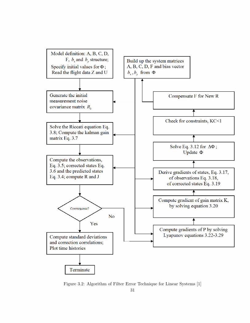
Figure 3.2: Algorithm of Filter Error Technique for Linear Systems [1]31
4. Apply the modified Newton-Raphson technique to minimize the cost function.
5. Update the parameter vector Φ.
6. Repeat the steps 3 - 5 until all parameters converge to specific and constant values.
3.1.5 Parameter Update
The modified Newton-Raphson method is applied in this section to update the param-
eter vector, Φ, such that it minimizes the cost function after each iteration. The following
equations were derived in section 2.4 [1].
Φi+1 = Φi + ∆Φ, where ∆Φ = −P1−1P2 (3.12)
P1 =∫ N
1
[∂y(tk)∂Φ
]TR−1
[∂y(tk)∂Φ
dt
](3.13)
P2 = −∫ N
1
[∂y(tk)∂Φ
]TR−1 [z(tk)− y(tk)] dt (3.14)
In the above equations, everything is readily available to use, except the sensitivity matrix
or the gradient matrix of response, given below [1]:
(∂y
∂Φ
)ij
=∂yi∂Φj
(3.15)
The sensitivity matrix ( ∂y∂Φ) can be solved using several ways. However, the classical method
is used in this thesis by solving the sensitivity equations [69]. The finite difference method
is also an excellent method, which is usually applied for nonlinear system. The required
32
sensitivity equations are obtained by differentiating the system equations with respect to
elements of the parameter matrix, Φ. Partial differentiation of Eq. 3.4 results in the
following equation [1].
∂x(tk+1)∂Φ
= Θ∂x(tk)∂Φ
+∂Θ∂Φ
x(tk) + Λ∂B
∂Φu(tk) +
∂Λ∂Φ
Bu(tk) + Λ∂bx∂Φ
+∂Λ∂Φ
bx (3.16)
The above equation is the exact gradient of Eq. 3.4 and is necessary to compute ∂Θ∂Φ and
∂Λ∂Φ . Maine and Iliff [67] eliminated this computation burden by approximating the gradient
computation significantly, explained below:
∂x(tk+1)∂Φ
≈ Θ∂x(tk)∂Φ
+ Λ∂A
∂Φx(tk) + Λ
∂B
∂Φu(tk) + Λ
∂bx∂Φ
,∂x(1)∂Φ
= 0 (3.17)
Two new terms are introduced in the above equations. An average of two consecutive
inputs is shown as u and x is an average of states at two successive time steps. Partial
differentiation of Eq. 3.5 and Eq. 3.6 result in the following equation [67].
∂y(tk)∂Φ
= C∂x(tk)∂Φ
+∂C
∂Φx(tk) +
∂D
∂Φu(t) +
∂by∂Φ
(3.18)
∂x(tk)∂Φ
=∂x(tk)∂Φ
−K∂y(tk)∂Φ
+∂K
∂Φ[z(tk)− y(tk)] (3.19)
Eqs. 3.17-3.19 represent a set of sensitivity equations. Except for the ∂K∂Φ all terms are
available at this point. Therefore, the gradient of the Kalman gain matrix is computed to
complete this optimization problem. Differentiate Eq. 3.7 to derive the following result
33

[67].
∂K
∂Φ=∂P
∂ΦCTR−1 + P
∂CT
∂ΦR−1 (3.20)
For each specific time step and at this stage in the algorithm measurement noise covariance
matrix R, system matrix C and state prediction error covariance matrix P are fixed and
constant. Partial differentiation of each element matrix C with respect to related parameters
is one and elsewhere it is zero. Thus, only ∂P∂Φ needs to be calculated to compute the gradient
of K. Note that ∂P∂Φ is a three dimensional matrix and hence ∂K
∂Φ is also a three dimensional
matrix. ∂P∂Φ is derived by differentiating the steady-state Riccati equation 3.8 [67].
A∂P
∂Φ+∂A
∂ΦP + P
∂AT
∂Φ+∂P
∂ΦAT − 1
∆t∂P
∂ΦCTR−1CP − 1
∆tP∂CT
∂ΦR−1CP
− 1∆t
PCTR−1∂C
∂Φ− 1
∆tPCTR−1C
∂P
∂Φ+ F
∂F T
∂Φ+∂F
∂ΦF T = 0 (3.21)
Arrange the left-hand side terms and simplify mathematically using matrix properties like
(A+B)T = AT +BT and (AB)T = BTAT . The result is shown here [67].
A∂P
∂Φ+∂P
∂ΦAT = C + C
T (3.22)
where
A = A− 1∆t
PCTR−1C = A− 1∆t
KC (3.23)
and
C = −∂A∂Φ
P +1
∆tPCTR−1∂C
∂ΦP − ∂F
∂ΦF T (3.24)
34
There is one equation like Eq. 3.22 for each element of the system parameter vector Φ.
This leads to a set of Lyapunov equations of the form AX + XAT = B [1, 67]. Since the
A matrix remains similar for the entire set, the Lyapunov equations are solved efficiently
utilizing the following transformation [67].
A′
= T−1AT (3.25)
and
(C + CT )
′= T−1(C + C
T )T ∗−1 (3.26)
Here, T is the matrix of the eigenvectors of A. Due to this alteration A′ is now diagonal
and thus Eq. 3.22 is left as [67]:
A′(∂P
∂Φ
)′
+(∂P
∂Φ
)′
A′∗ = (C + C
T )′
(3.27)
As the A′ is diagonal, the above equation can be solved for(∂P∂Φ
)′
easily. Generally for a
diagonal matrix A, AX +XAT = B can be solved by [67]
Xij =Bij
(Aii +Ajj)(3.28)
The gradient of the state prediction error covariance matrix P is calculated using back
transformation [67].
∂P
∂Φ= T
(∂P
∂Φ
)′
T ∗ (3.29)
35
Now, Eqs. 3.12-3.14 can be solved easily. As stated earlier, this technique leads to an
unconditional minimum of the cost function. All system parameters are treated separately.
The results obtained using this technique will be provided and discussed in the next chapter.
3.2 Filter Error Technique for Non-linear Systems
The general mathematical model of a non-linear system is given below:
x(t) = f [x(t), u(t), β] + Fw(t), x(t0) = x0 (3.30)
y(t) = g[x(t), u(t), β] (3.31)
z(tk) = y(t) +Gv(tk) (3.32)
Here f and g are nonlinear functions, x(t) is a state vector and u(t) is an input vector. F
and G are time-invariant noise distribution matrices.
The filter error technique for nonlinear systems is illustrated in Fig. 3.3. For non-linear
systems, response gradients are calculated based on finite difference approximations. An
extended Kalman filter [77, 78] dependent on the first-order approximation of the dynamical
equations is used for non-linear filtering.
36

Figure 3.3: Algorithm of Filter Error Technique for Nonlinear Systems [1]
37

3.2.1 Steady State Filter
The combined formulation is followed, for the nonlinear case just as was done for the
linear case. The two-step relation strategy, discussed in section 2.4 is applied to estimate
R. While doing this, the following tasks are important.
1. Select some suitable initial values for the unknown parameter vector Φ. Load the
available flight data (from real time flight or from simulator).
2. Apply the extended Kalman filter and calculate the observation vector, Y; innovation
matrix; initial measurement noise covariance matrix, R; and the initial cost function,
J. Numerically integrate the state equations. For numerical integration, a fourth order
Runge-Kutta method was used. A description of this method is given in appendix B.
3. Solve the Riccati equation and find the new Kalman gain. Calculate a new measure-
ment noise covariance matrix, R, and new cost function, J.
4. Apply the modified Newton-Raphson technique to minimize the cost function.
5. Update the parameter vector, Φ.
6. Repeat steps 3 - 5 until all parameters converge to constant values.
The optimal filters are practically impossible for non-linear systems. Hence, an extended
Kalman filter is used here. A two-step, non-linear, constant-gain filter is formulated as [1].
38

Prediction step
x(tk+1) = x(tk) +∫ tk+1
tk
f [x(t), u(t), β]dt, x(t0) = x0 (3.33)
y(tk) = g[x(t), u(t), β] (3.34)
Correction step
x(tk) = x(tk) +K[z(tk)− y(tk)] (3.35)
The Kalman gain K is dependent on the measurement noise covariance matrix, R, state
prediction error covariance matrix, P; and system matrix, C. It is expressed as [1]:
K = PCTR−1 (3.36)
where
C =[∂g[x(t), u(t), β]
∂x
]t=t0
(3.37)
A steady-state, continuous-time, Riccati equation is solved here to calculate P . The lin-
earized matrices A and C are used, and solved using a finite difference method which is
explained below.
Finite Difference Technique:
39
If each of the state variables is perturbed by δxj , the elements of the matrices A and
C can be approximated using a central difference formula as [1]:
Aij ≈(fi[x+ δxj , u, β]− fi[x− δxj , u, β]
2δxj
)x=x0
(3.38)
Cij ≈(gi[x+ δxj , u, β]− gi[x− δxj , u, β]
2δxj
)x=x0
(3.39)
For the non-linear system, the response gradients are approximated using the finite differ-
ence approximation. For a small perturbation δΦj in each variable of the unknown param-
eter vector Φ, the perturbed response variable yp for each of the unperturbed variable yi is
computed. The sensitivity response gradient is approximated as
[∂y(tk)∂Φ
]=yp(tk)− yi(tk)
δΦ(3.40)
For each element of the unknown parameter vector, Φ, the state and observation vari-
ables are calculated utilizing a two step non-linear steady-state filter as given below [1].
Prediction step
xp−j(tk+1) = xp−j(tk) +∫ tk+1
tk
f [xp−j(tk+1), u(tk+1), β + δβjej ]dt (3.41)
yp−j(tk) = g[xp−j(tk+1), u(tk+1), β + δβjej ] (3.42)
40
Correction step
xp−j(tk) = xp−j(tk) +Kp−j [z(tk)− yp−j(tk)] (3.43)
The predicted state variables x in Eq. 3.41 are computed by numerical integration. To
compute Eq. 3.43 the perturbed Kalman gain matrix Kp−j needs to be calculated, which
is given by [1]
Kp−j = Pp−jCTp−jR
−1 (3.44)
here, the perturbed system matrices Ap−j and Cp−j need to be calculated to use them to
solve the Riccati equation, which are approximated using a central difference method.
3.2.2 Parameter Update
Referring to section 3.1.5 and Eqs. 3.13-3.14, all quantities can be derived for non-
linear systems. The parameter vector Φ will be updated using Eq. 3.12. This technique
also leads to an unconditional minimum of the cost function. The results obtained using
this technique will be provided and discussed in the next chapter.
41
Chapter 4
Prediction of Aircraft Stability and Control Derivatives
Techniques to calculate the stability and control derivatives analytically, are presented
in this chapter. These derivatives are an important part of the experiment because they
are required as an input to determine dynamic stability and control behavior [79]. These
methods are referred from [79-83]. Only preliminary information is presented here. Details
should be found from [79-83]. Stability and control derivatives given in Eqs. 5.1-5.5 are
predicted using the following methods. Initial values derived using these methods were used
in the experimental aircraft Trainer.
The important notes while using these methods are [79]:
1. The methods presented in this chapter apply only to rigid aircraft.
2. The methods presented in this chapter apply only to subsonic speed regimes.
3. All derivatives are in rad−1.
4. All coefficients and derivatives are defined in the stability axes system.
5. The drag prediction methods apply only in the flight cases where the boundary layer
is turbulent.
6. The drag prediction methods apply only to smooth surfaces.
42

4.1 Steady State Coefficients
The definitions of steady state coefficients CD, CL and Cm0 are given below. They
were used to determine the lift, drag and pitching moment steady state coefficients [79].
CL is the aircraft’s steady-state lift coefficient, given as [79]:
CL = W/(qS) (4.1)
CD is the aircraft’s steady-state drag coefficient. It is calculated using the following
method. As shown in Fig. 4.1, it is related to a specific value of steady-state lift coefficient
CL. The steady-state aircraft drag coefficient is given as follows [79]:
CD = CDw + CDfus (4.2)
The wing drag coefficient is predicted from [79]:
CDw = CD0w+ CDLw
where CD0w= (Rwf )(RLS)(Rfw){1 + L′(t/c) + 100(t/c)4}(Swet/S)
and CDLw = (CLw)2/πAe+ 2πCLwηtv + 4π2(ηt)2w (4.3)
43

Figure 4.1: Determination of Drag Coefficient from a known Lift Coefficient
The fuselage drag coefficient is predicted from [79]:
CDfus = CD0fus+ CDLfus
where CD0fus= (Rwf )(Cffus){1 + 60(lf/df )3 + 0.0025(lf/df )}(Swet/S) + CDbfus
and CDLfus = 2α2(Sb/S) + ηcdcα3(Splffus/S) (4.4)
Cm0 is the aircraft zero lift pitching moment coefficient and can be predicted using the
following equation [79]:
Cm0 = Cm0wf+ Cm0h
(4.5)
44

Cm0wfis the zero lift pitching moment coefficient due to wing-fuselage combination. It is
predicted from [79]:
Cm0wf= {(Cm0w
)+(Cm0f)}{(Cm0)M+(Cm0)M=0}
where Cm0w= {(Acos2Λc/4)/(A+2cosΛc/4)}(cm0r
+cm0t)/2
+(∆Cm0/εt)εt
and Cm0f= {(k2−k1)/36.5Sc}[
∑{(wfi
2)(iw+α0Lw+iclf )∆xi}] (4.6)
Cm0his the zero lift pitching moment coefficient because of the horizontal tail. It is predicted
from [79]:
Cm0h= −(xach−xref )CL0h
(4.7)
4.2 Stability Derivatives
The techniques for calculating the following stability derivatives are addressed in this
section:
1. Aircraft speed derivatives.
2. Angle of attack derivatives.
3. Angle of sideslip derivatives.
4. Roll rate derivatives.
45

5. Pitch rate derivatives.
6. Yaw rate derivatives.
As it was stated before, only preliminary equations are addressed here. Complete analysis
can be found in [79-83].
4.2.1 Aircraft Speed Derivatives
The aerodynamic speed derivative CLV , lift with respect to aircraft speed is determined
using the following equation [79].
CLV = {M2(cosΛc/4)2CL}/{1−M2(cosΛc/4)2} (4.8)
The aerodynamic speed derivative CDV , drag with respect to aircraft speed is deter-
mined using the following equation [79].
CDV = M(∂CD/∂M) (4.9)
The aerodynamic speed derivative CmV , pitching moment with respect to aircraft speed
is determined using the following equation [79].
CmV = −CL(∂XacA/∂M) (4.10)
46

4.2.2 Angle of Attack Derivatives
The derivative of the aerodynamic lift with respect to aircraft angle of attack (also
called as the aircraft lift curve slope) can be determined from [79]:
CLα = CLαwf + CLαhηh(Sh/S)(1− dε/dα) (4.11)
CLαwf is the wing-fuselage lift curve slope, determined as [79]:
CLαwf = KwfCLαw (4.12)
where CLαw is the wing lift curve slope and is given by [79]:
CLαw = 2πA/[2 + {(A2β2/k2)(1 + tan2Λc/2/β2) + 4}1/2] (4.13)
CLαh is the horizontal tail lift curve slope. It can be calculated using the above equation
with suitable substitution of horizontal tail parameters for the wing parameters. All other
quantities in Eqs. 4.11-4.13 are defined in [79].
The derivative of the aerodynamic drag with respect to aircraft angle of attack can be
computed as follows [79].
CDα = (∂CD/∂CL)CLα (4.14)
47
The derivative of the aerodynamic pitching moment with respect to aircraft angle of
attack can be calculated as follows [79].
Cmα = (∂Cm/∂CL)CLα (4.15)
4.2.3 Angle of Sideslip Derivatives
The aircraft equations of motion contain the aerodynamic pitch velocity derivatives
Lv, Nv, Yv. They are derivatives of rolling moment, yawing moment and side force with
respect to pitch velocity. If the angle of sideslip is very small then it is given by:
β = v/u (4.16)
From the above equation:
Lβ = Lvu
Nβ = Nvu
Yβ = Yvu (4.17)
48

Lβ, Nβ and Yβ are calculated first to predict Lv, Nv and Yv and given as [83],
Lβ =qSbClβIx
Nβ =qSbCnβIz
Yβ =qSCyβm
(4.18)
The theoretical methods to predict the coefficients given in the above equations are
described in this section.
The coefficient of the rolling moment derivative with respect to the sideslip, Clβ (also
called the dihedral effect) can be calculated from [79]:
Clβ = Clβwf + Clβh + Clβv (4.19)
The wing-fuselage contribution is given by [79]:
Clβwf =180π
[CLwf {(Clβ/CL)Λc/2(KMΛ)(Kf )+(Clβ/CL)A}
+Γ{(Clβ/Γ)KMΓ+(∆Clβ/Γ)}+(∆Clβ )zw
+(εttanΛc/4){(∆Clβ )/(εttanΛc/4)}] (4.20)
The horizontal and vertical tail contributions are given by [79]:
Clβh = (Clβhf )(Shbh/Sb)
49

Clβv = (Cyβv ){(zvcosα−lvsinα)/b} (4.21)
The coefficient of the yawing moment derivative with respect to the sideslip, Cnβ (also
called static dihedral stability) is computed from [79]:
Cnβ = Cnβw + Cnβf + Cnβv (4.22)
The wing, fuselage and vertical tail contributions are given in order as [79]:
Cnβw = 0
Cnβf =−180pi
KNKR1(Sfsbf/Sb)
Cnβv = −(Cyβv ){(lvcosα+zvsinα)/b} (4.23)
The coefficient of the side force derivative with respect to the sideslip, Cyβ is calculated
from [79]:
Cyβ = Cyβw + Cyβf + Cyβv (4.24)
The wing, fuselage and vertical tail contributions are given in order as [79]:
Cyβw = −0.00573(|Γ|)
Cyβf = −2Ki(Scs/S)
50
Cyβv = −kv(CLαv )(1+dσ/dβ)ηv(Sv/S) (4.25)
4.2.4 Roll Rate Derivatives
The rolling moment with respect to the roll rate is [83],
Lp =qSb2Clp2Ixu0
The coefficient of the rolling moment with respect to the roll rate Clp , also called the
damping derivative, is found from [79]:
Clp = Clpw+Clph+Clpv (4.26)
The wing, horizontal and vertical tail contributions are given in order as [79]:
Clpw = (βClp/k)CL=0(k/β){(CLαw )CL/(CLαw )CL=0}∗
∗{(Clp)Γ/(Clp)Γ=0}+ (∆Clp)drag
Clph = 0.5(Clp)h(Sh/S)(bh/b)2
Clpv = 2(zv/b)2Yβv (4.27)
The derivative of the yawing moment with respect to the roll rate is [83],
Np =qSb2Cnp
2Izu0
51

The derivative of the coefficient of the yawing moment with respect to the roll rate, Cnp , is
found from [79]:
Cnp = Cnpw+Cnpv (4.28)
The wing and vertical tail contributions are given in order as [79]:
Cnpw = {(Cnp/CL)CL=0}CL+(Cnp/εt)εt
+[∆Cnp/{(αδf )(δf )}](αδf )(δf )
Cnpv = −(2/b2)(lvcosα+zvsinα)(zvcosα−lvsinα−zv)Cyβv (4.29)
The derivative of the side force with respect to the roll rate is [83],
Yp =qSbCnp2mu0
The derivative of the coefficient of the side force with respect to the roll rate Cyp can be
found from [79]:
Cyp = 2(Cyβv ){(zvcosα−lvsinα)/b} (4.30)
52
4.2.5 Pitch Rate Derivatives
The pitching moment with respect to pitch rate derivative, also called pitch damping
derivative is calculated from [79]:
Cmq = Cmqw + Cmqh (4.31)
The wing contribution is given by [79]:
Cmqw = Cmqw/at M=0{A3tan2Λc/4AB+6cosΛc/4
+3B}/{
A3tan2Λc/4A+6cosΛc/4
+3}
where Cmqw/at M=0= −kwClαw cosΛc/4[
A{2(xw/c)2+0.5(xw/c)}(A+2cosΛc/4)
+A3tan2Λc/4
24(A+6cosΛc/4)+
18
]
The horizontal tail contribution is given by [79]:
Cmqh = −2(CLαh )ηhV h(xach−xcg) (4.32)
4.2.6 Yaw Rate Derivatives
The derivative of the rolling moment with respect to the yaw rate is [83],
Lr =qSb2Clr2Ixu0
53

The coefficient of the rolling moment with respect to the yaw rate Clr is determined
from [79]:
Clr = Clrw+Clrv (4.33)
The wing and vertical tail contributions are given in order as [79]:
Clrw = (CLw)(Clr/CL)CL=0+(∆Clr/Γ)Γ+(∆Clr/εt)εt
+[∆Clr/{(αδf )(δf )}](αδf )(δf )
Clrv = −(2/b2)(lvcosα+zvsinα)(zvcosα−lvsinα)Cyβv (4.34)
The yawing moment with respect to the yaw rate is [83],
Nr =qSb2Cnr
2Izu0
The coefficient of the yawing moment with respect to the yaw rate Cnr , also called the
yaw damping is found from [79]:
Cnr = Cnrw+Cnrv (4.35)
The wing and vertical tail contributions are given in order as [79]:
Cnrw = (Cnr/CL2)(CLw)2+(Cnr/CD0)CD0w
54

Cnrv = (2/b2)(lvcosα+zvsinα)2Cyβv (4.36)
The side force with respect to the yaw rate is [83],
Yr =qSbCyr2mu0
The coefficient of the side force with respect to the yaw rate Cyr , is found from [79]:
Cyr = −2(Cyβv ){(lvcosα+zvsinα)/b} (4.37)
4.3 Control Derivatives
The techniques to calculate the following control derivatives are addressed in this sec-
tion:
1. Aileron control derivatives.
2. Elevator control derivatives.
3. Rudder control derivatives.
As it was stated before, only preliminary equations are addressed here. Complete analysis
can be found from [79-83].
55
4.3.1 Aileron Control Derivatives
The rolling moment with respect to the aileron deflection is given as [83]
Lδa =qSbClδaIx
The coefficient of the rolling moment with respect to the aileron deflection, Clδa , also
called the roll control power, is calculated from [83]:
Clδa =2CLαw τSb
∫ y2
y1
cy dy (4.38)
The yawing moment with respect to the aileron deflection is given as [83]
Nδa =qSbCnδa
Iz
The coefficient of the yawing moment with respect to the aileron deflection, Cnδa , also
called the adverse aileron yaw, is predicted from [83]:
Cnδa = KaCLwClδa (4.39)
The side force with respect to the aileron deflection is given as [83]
Yδa =qSCyδam
56
The coefficient of the side force with respect to the aileron deflection, Cyδa is negligible
for most of the conventional aileron arrangements [80]:
Cyδa = 0 (4.40)
4.3.2 Elevator Control Derivatives
The pitching moment with respect to elevator derivative, Cmδe , also called the elevator
control power, can be found from [79]:
Cmδe = (αδe)Cmih
(αδe) = kb{clδ/(clδ)theory}(clδ)theory(k′/clαh )[(αδ)CL/(αδ)cl ]
Cmih = −(CLαh )ηhV h (4.41)
4.3.3 Rudder Control Derivatives
The rolling moment with respect to the rudder deflection is given as [83]
Lδr =qSbClδrIx
The coefficient of the rolling moment with respect to the aileron deflection, Clδr , also
called the roll control power, is calculated from [83]:
Clδr = {(zvcosα−lvsinα)/b}Cyβv (4.42)
57
The yawing moment with respect to the rudder deflection is given as [83]
Nδr =qSbCnδr
Iz
The coefficient of the yawing moment with respect to the aileron deflection, Cnδr , also
called the rudder control power, can be found from [79]:
Cnδr = −Cyβv {(lvcosα+zvsinα)/b} (4.43)
The side force with respect to the rudder deflection is given as [83]
Yδr =qSCyδrm
The coefficient of the side force with respect to the rudder deflection, Cyδr is given as
[79]:
Cyδr = (CLαv )(k′Kb){(αδ)CL/(αδ)Cl}(αδ)Cl(Sv/S) (4.44)
58

Chapter 5
Investigated Examples of System Identification Using Flight Test Data
Two separate experiments were performed to investigate the System Identification the-
ory, which was detailed in Chapters 2 and 3. The filter error technique was used in both
experiments.
Sections 5.1-5.2 provide experimental details, which were originally carried out at
DFVLR, Institute of Flight Mechanics, Braunschweig, Federal Republic of Germany [68].
The first experiment of this thesis utilized the same flight parameters and flight test data,
which were used in the original experiments. The results of the experiments and compar-
ison with the earlier experiments [1, 68] are also presented. The second experiment was
performed on a radio controlled, glow-powered aircraft trainer, the Hanger 9 Extra Easy.
The flight test data were acquired at Auburn University, Auburn, AL, USA.
5.1 Estimation of Lateral Motion Derivatives using the Simulated Flight Data
This experiment was performed to estimate the lateral motion derivatives of an aircraft
using a linear model and simulated aircraft response. The aircraft response was generated
incorporating moderate to high level of turbulence [1]. Nominal values of the lateral motion
aerodynamic derivatives used correspond to those obtained by parameter estimation from
flight data recorded during the tests in a steady atmosphere with the research aircraft de
Havilland DHC-2, shown in Fig. 5.1 [68]. Classical equations of aircraft motion including
59
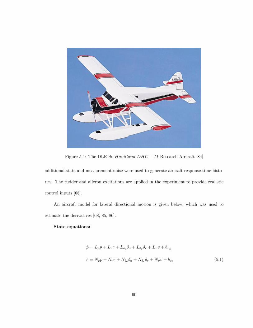
Figure 5.1: The DLR de Havilland DHC − II Research Aircraft [84]
additional state and measurement noise were used to generate aircraft response time histo-
ries. The rudder and aileron excitations are applied in the experiment to provide realistic
control inputs [68].
An aircraft model for lateral directional motion is given below, which was used to
estimate the derivatives [68, 85, 86].
State equations:
p = Lpp+ Lrr + Lδaδa + Lδrδr + Lvv + bxp
r = Npp+Nrr +Nδaδa +Nδrδr +Nvv + bxr (5.1)
60
Observation equations:
pm = Lpp+ Lrr + Lδaδa + Lδrδr + Lvv + byp
rm = Npp+Nrr +Nδaδa +Nδrδr +Nvv + byr
aym = Ypp+ Yrr + Yδaδa + Yδrδr + Yvv + byay
pm = p+ byp
rm = r + byr (5.2)
The unknown parameter vector Φ for the considered model has dimensional derivatives and
bias terms. It is given as [68]:
ΦT = [Lp Lr Lδa Lδr Lv Np Nr Nδa Nδr Nv Yp Yr
Yδa Yδr Yv bxp bxr byp byr byay byp byr fpp frr] (5.3)
Each element of the parameter vector Φ is defined in the above equations except fpp and
frr. They form diagonal process noise distribution matrix F. The initial values were kept
the same as they were in the original experiment [68].
5.1.1 Comparison of the Results with the Original Experiment
The estimated results for the lateral motion derivatives, applying the system identifi-
cation techniques discussed in Chapters 2 and 3, are summarized in Table 5.1. Initial and
nominal values of the derivatives [1] are also given in the table. The results obtained from
61
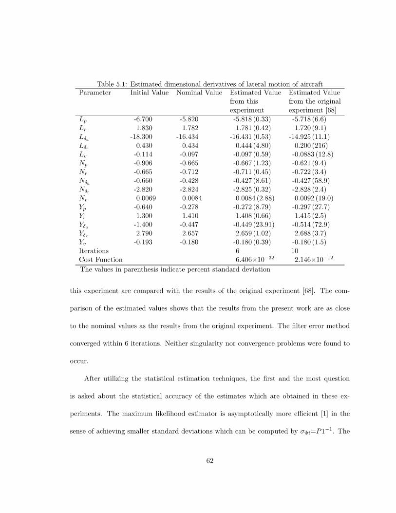
Table 5.1: Estimated dimensional derivatives of lateral motion of aircraftParameter Initial Value Nominal Value Estimated Value Estimated Value
from this from the originalexperiment experiment [68]
Lp -6.700 -5.820 -5.818 (0.33) -5.718 (6.6)Lr 1.830 1.782 1.781 (0.42) 1.720 (9.1)Lδa -18.300 -16.434 -16.431 (0.53) -14.925 (11.1)Lδr 0.430 0.434 0.444 (4.80) 0.200 (216)Lv -0.114 -0.097 -0.097 (0.59) -0.0883 (12.8)Np -0.906 -0.665 -0.667 (1.23) -0.621 (9.4)Nr -0.665 -0.712 -0.711 (0.45) -0.722 (3.4)Nδa -0.660 -0.428 -0.427 (8.61) -0.427 (58.9)Nδr -2.820 -2.824 -2.825 (0.32) -2.828 (2.4)Nv 0.0069 0.0084 0.0084 (2.88) 0.0092 (19.0)Yp -0.640 -0.278 -0.272 (8.79) -0.297 (27.7)Yr 1.300 1.410 1.408 (0.66) 1.415 (2.5)Yδa -1.400 -0.447 -0.449 (23.91) -0.514 (72.9)Yδr 2.790 2.657 2.659 (1.02) 2.688 (3.7)Yv -0.193 -0.180 -0.180 (0.39) -0.180 (1.5)Iterations 6 10Cost Function 6.406×10⁻³² 2.146×10⁻¹²
The values in parenthesis indicate percent standard deviation
this experiment are compared with the results of the original experiment [68]. The com-
parison of the estimated values shows that the results from the present work are as close
to the nominal values as the results from the original experiment. The filter error method
converged within 6 iterations. Neither singularity nor convergence problems were found to
occur.
After utilizing the statistical estimation techniques, the first and the most question
is asked about the statistical accuracy of the estimates which are obtained in these ex-
periments. The maximum likelihood estimator is asymptotically more efficient [1] in the
sense of achieving smaller standard deviations which can be computed by σΦi=P1−1. The
62

asymptotic efficiency is an important property with practical importance. It implies that
the maximum likelihood estimator makes efficient use of the available data and that the
smaller standard deviation indicates theoretically maximum achievable accuracy of the es-
timates [1]. Tables 5.1-5.5 indicate that the standard deviation of all estimated derivatives
are smaller, which means the estimates are very accurate.
5.1.2 Responses and Results
The comparison of the estimated model response with the measured data and the time
history plots of the control inputs are shown in Fig. 5.2. As it was stated before, the control
inputs and flight data used in this experiment are same as the original experiment [68]. The
estimated data are shown in green while the measured data are shown as blue. Fig. 5.3
shows the convergence plots of the estimated parameters, which suggest all parameters are
converging to a specific constant value within 6 iterations.
Reduction of the cost function appears in Fig. 5.4, which shows how rapidly the cost
function reduces. This is due to the modified Newton-Raphson technique, which finds zero
for the gradient of the cost function at the local minimum point. Also, the theoretically
predicted parameters are very close to the estimated parameters using the algorithm. This
is the prime reason the cost function is very small. Recalling the formulations for process
noise discussed in Section 3.1.2, the combined formulation was used in this experiment.
From Table 5.1 and Figs. 5.2-5.4 the following points are observed.
1. The measured response and the estimated response are in agreement with each other.
63

Figure 5.2: Comparison of Estimated(green) and Measured(blue) Responses for the LateralDirectional Motion of Aircraft
64

Figure 5.3: Convergence Plots of Dimensional Derivatives for Lateral Directional Motion ofAircraft
65
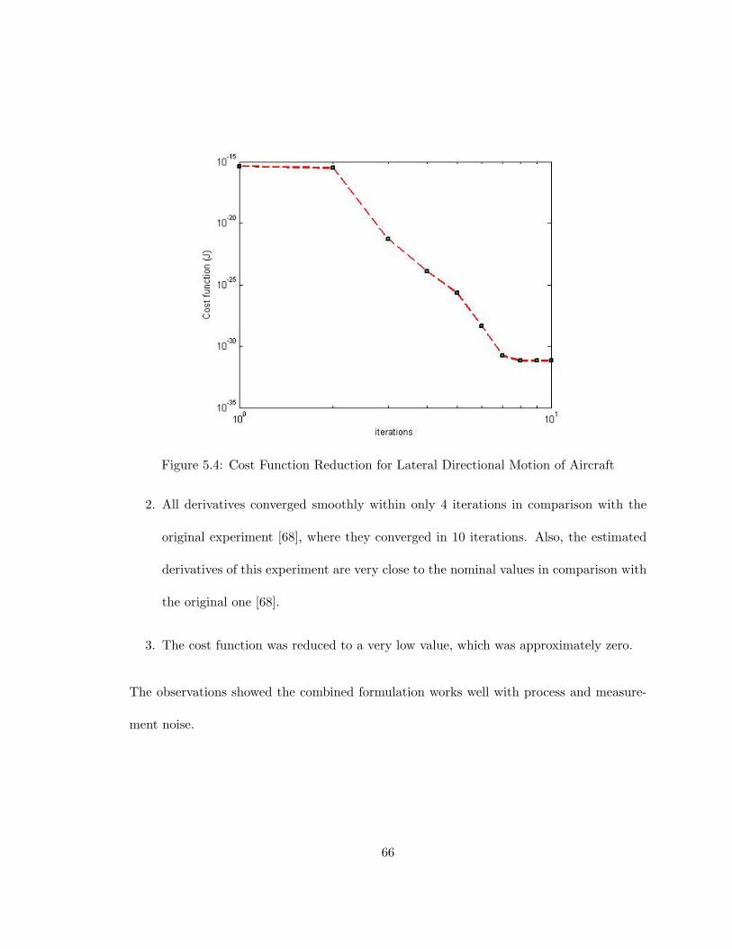
Figure 5.4: Cost Function Reduction for Lateral Directional Motion of Aircraft
2. All derivatives converged smoothly within only 4 iterations in comparison with the
original experiment [68], where they converged in 10 iterations. Also, the estimated
derivatives of this experiment are very close to the nominal values in comparison with
the original one [68].
3. The cost function was reduced to a very low value, which was approximately zero.
The observations showed the combined formulation works well with process and measure-
ment noise.
66

Figure 5.5: The DLR HFB − 320 Research Aircraft [87]
5.2 Estimation of Longitudinal Motion Derivatives of HFB-320 Aircraft
This experiment was performed to estimate the non dimensional derivatives of another
aircraft. A non-linear model of a fixed wing research aircraft, the HFB-320, shown in Fig.
5.5, was used and the drag, lift and pitching moment coefficients of this research aircraft
were estimated [87]. The longitudinal motion of the aircraft was excited through flight tests
[88]. A multi-step elevator input was used in the flight test, which resulted in a short period
motion, as well as a pulse input, that lead to a phugoid motion [89]. The inputs are shown
in Fig. 5.8.
A non-linear model of longitudinal motion of aircraft was utilized in the experiment
because the non-linear model was found to provide excellent estimation results [88-90]. The
postulated non-linear model to estimate the non-dimensional aerodynamic derivatives is
67
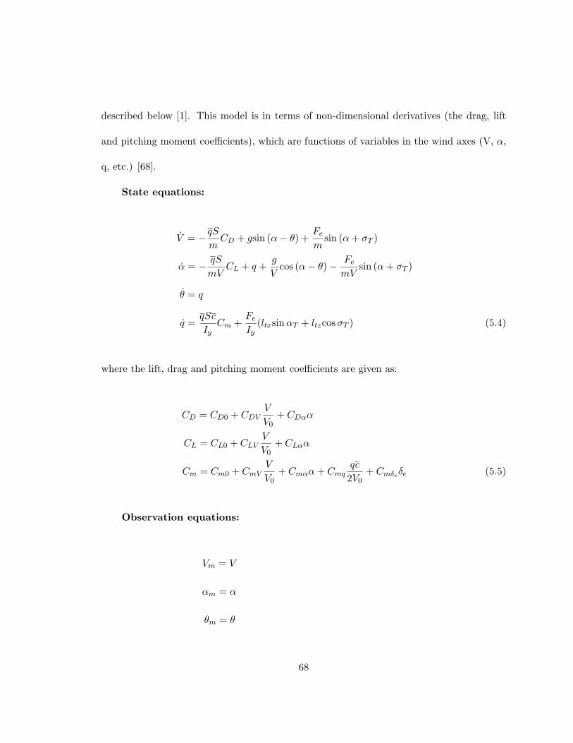
described below [1]. This model is in terms of non-dimensional derivatives (the drag, lift
and pitching moment coefficients), which are functions of variables in the wind axes (V, α,
q, etc.) [68].
State equations:
V = −qSmCD + gsin (α− θ) +
Fem
sin (α+ σT )
α = − qS
mVCL + q +
g
Vcos (α− θ)− Fe
mVsin (α+ σT )
θ = q
q =qSc
IyCm +
FeIy
(ltxsinαT + ltzcosσT ) (5.4)
where the lift, drag and pitching moment coefficients are given as:
CD = CD0 + CDVV
V0+ CDαα
CL = CL0 + CLVV
V0+ CLαα
Cm = Cm0 + CmVV
V0+ Cmαα+ Cmq
qc
2V0+ Cmδeδe (5.5)
Observation equations:
Vm = V
αm = α
θm = θ
68
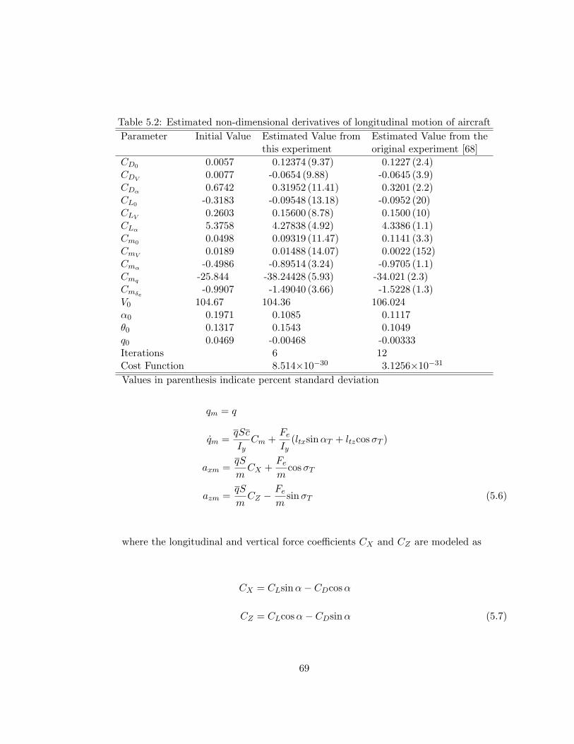
Table 5.2: Estimated non-dimensional derivatives of longitudinal motion of aircraftParameter Initial Value Estimated Value from Estimated Value from the
this experiment original experiment [68]CD0 0.0057 0.12374 (9.37) 0.1227 (2.4)CDV 0.0077 -0.0654 (9.88) -0.0645 (3.9)CDα 0.6742 0.31952 (11.41) 0.3201 (2.2)CL0 -0.3183 -0.09548 (13.18) -0.0952 (20)CLV 0.2603 0.15600 (8.78) 0.1500 (10)CLα 5.3758 4.27838 (4.92) 4.3386 (1.1)Cm0 0.0498 0.09319 (11.47) 0.1141 (3.3)CmV 0.0189 0.01488 (14.07) 0.0022 (152)Cmα -0.4986 -0.89514 (3.24) -0.9705 (1.1)Cmq -25.844 -38.24428 (5.93) -34.021 (2.3)Cmδe -0.9907 -1.49040 (3.66) -1.5228 (1.3)V0 104.67 104.36 106.024α0 0.1971 0.1085 0.1117θ0 0.1317 0.1543 0.1049q0 0.0469 -0.00468 -0.00333Iterations 6 12Cost Function 8.514×10⁻³⁰ 3.1256×10⁻³¹
Values in parenthesis indicate percent standard deviation
qm = q
qm =qSc
IyCm +
FeIy
(ltxsinαT + ltzcosσT )
axm =qS
mCX +
Fem
cosσT
azm =qS
mCZ −
Fem
sinσT (5.6)
where the longitudinal and vertical force coefficients CX and CZ are modeled as
CX = CLsinα− CDcosα
CZ = CLcosα− CDsinα (5.7)
69

The above mentioned non-linear aircraft model of Eqs. 5.4-5.6, contains non-linearities due
to trigonometric terms, q and also on account of the transformation in Eq. 5.7.
The unknown parameter vector Φ for the considered model has non-dimensional deriva-
tives, and is given below as [1]:
ΦT = [CD0 CDV CDα CL0 CLV CLα Cm0 CmV Cmα Cmq Cmδe ] (5.8)
5.2.1 Comparison of the Results with the Original Experiment
The estimated results from the longitudinal motion derivatives, applying the system
identification technique discussed in Chapters 2 and 3, are summarized in the Table 5.2.
Initial values of the non-dimensional derivatives [1] are also given in the table. The results
obtained from this experiment are compared with the results of the original experiment
[68]. Neither singularity nor convergence problems were found to occur in this experiment.
5.2.2 Responses and Results
The comparison of the estimated model response with the measured data and the time
history plots of the control inputs are shown in Fig. 5.6. The estimated data are shown
in green while the measured data are shown in blue. Fig. 5.7 shows the convergence plots
of the estimated parameters, which suggest all derivatives converged smoothly within only
4 iterations in comparison with the original experiment [68], where they converged in 12
70
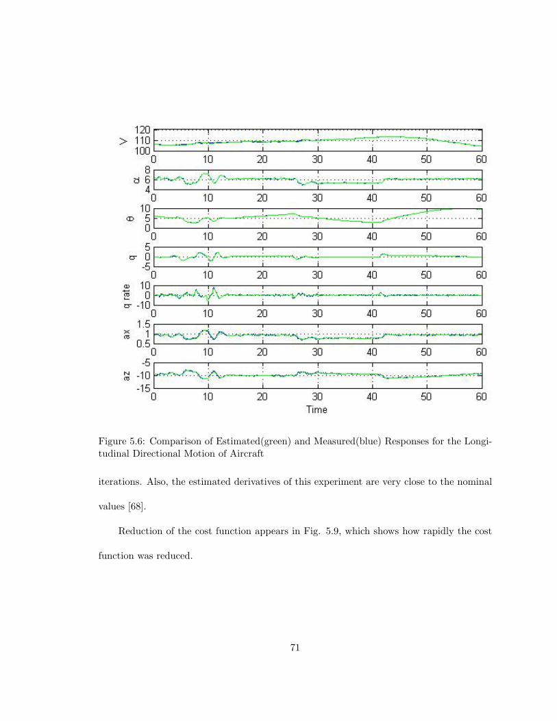
Figure 5.6: Comparison of Estimated(green) and Measured(blue) Responses for the Longi-tudinal Directional Motion of Aircraft
iterations. Also, the estimated derivatives of this experiment are very close to the nominal
values [68].
Reduction of the cost function appears in Fig. 5.9, which shows how rapidly the cost
function was reduced.
71
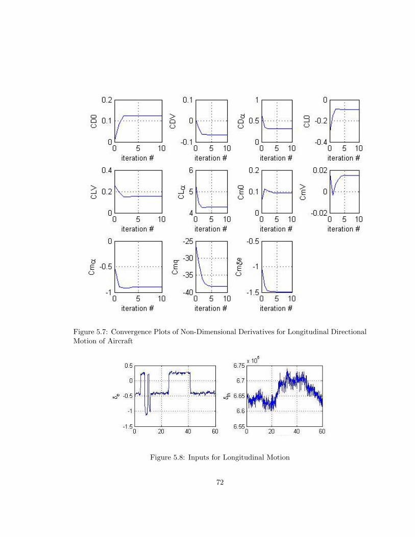
Figure 5.7: Convergence Plots of Non-Dimensional Derivatives for Longitudinal DirectionalMotion of Aircraft
Figure 5.8: Inputs for Longitudinal Motion
72

Figure 5.9: Cost Function Reduction for Longitudinal Motion
5.3 System Identification Applied to Model Aircraft Trainer
The experiments discussed in sections 5.1-5.2 were successfully completed. As a final
part of the exercise, the system identification technique was applied to model aircraft trainer.
The filter error technique for linear and nonlinear systems discussed in Chapter 3 were
applied here, as well as the modified Newton-Raphson algorithm to reduce the cost function.
The experiment and results are discussed in the following subsections.
5.3.1 The Investigated Aircraft Trainer - Hanger 9 Extra Easy
An unmanned aerial aircraft trainer, Hanger 9 Extra Easy which is made by Hobby
Outlet (shown in Fig. 5.10), was investigated in the third experiment. The Hanger 9 Extra
73

Figure 5.10: Aircraft Trainer - Hanger 9 Extra Easy [91]
Easy is a radio controlled glow powered aircraft. Both, lateral and longitudinal motion
derivatives were estimated for this aircraft. For lateral directional motion, a linear model
was used and the state and observation equations of Eqs. 5.1-5.2 were utilized. The unknown
parameter vector Φ of Eq. 5.3 was estimated. For longitudinal directional motion, a non-
linear model was used and the state and observation equations of Eqs. 5.4-5.7 were utilized.
The unknown parameter vector Φ of Eq. 5.8 was estimated. The aerodynamic, geometric
and mass details of the trainer aircraft [91] are given in the following Table 5.3. Geometric
details were provided by the manufacturer and the remaining details were measured from
the aircraft.
5.3.2 Responses and Results
The stability and control derivatives of the aircraft trainer, given in Eq. 5.3 and
Eq. 5.8 were estimated in this part of experiment. The initial value of each derivative
74
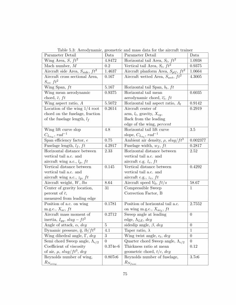
Table 5.3: Aerodynamic, geometric and mass data for the aircraft trainerParameter Detail Data Parameter Detail DataWing Area, S, ft2 4.8472 Horizontal tail Area, St, ft2 1.0938Mach number, M 0.2 Vertical tail Area, St, ft2 0.9375Aircraft side Area, Sside, ft2 1.4637 Aircraft planform Area, Splf , ft2 1.0664Aircraft cross sectional Area, 0.167 Aircraft wetted Area, Swet, ft2 4.3005Scs, ft2
Wing Span, ft 5.167 Horizontal tail Span, bt, ftWing mean aerodynamic 0.9375 Horizontal tail mean 0.6035chord, c, ft aerodynamic chord, ct, ftWing aspect ratio, A 5.5072 Horizontal tail aspect ratio, At 0.9142Location of the wing 1/4 root 0.2614 Aircraft center of 0.2919chord on the fuselage, fraction arm, lt, gravity, Xcg,of the fuselage length, lf Back from the leading
edge of the wing, percentWing lift curve slop 4.8 Horizontal tail lift curve 3.5CLαw , rad−1 slope, CLαt , rad
−1
Span efficiency factor, e 0.75 Ambient air density, ρ, slug/ft3 0.002377Fuselage length, lf , ft 4.2917 Fuselage width, wf , ft 0.2817Horizontal distance between 2.33 Horizontal distance between 2.52vertical tail a.c. and vertical tail a.c. andaircraft wing a.c., lp, ft aircraft c.g. lv, ftVertical distance between 0.145 Vertical distance between 0.4292vertical tail a.c. and vertical tail a.c. andaircraft wing a.c., zp, ft aircraft c.g., zv, ftAircraft weight, W , lbs 8.64 Aircraft speed V0, ft/s 58.67Center of gravity location, 31 Compressible Sweep 1percent of c, Correction Factor, Bmeasured from leading edgePosition of a.c. on wing 0.1781 Position of horizontal tail a.c. 2.7552m.g.c., Xac, ft on wing m.g.c., Xach , ftAircraft mass moment of 0.2712 Sweep angle at leading 0inertia, Iyy, slug − ft2 edge, ΛLE , degAngle of attack, α, deg 5 sideslip angle, β, deg 0Dynamic pressure, q, lb/ft2 4.1 Taper ratio, λ 1Wing dihedral angle, Γ, deg 3 Wing twist angle, εt, deg 0Semi chord Sweep angle, Λc/2 0 Quarter chord Sweep angle, Λc/2 0Coefficient of viscosity 0.374e-6 Thickness ratio at mean 0.12of air, µ, slug/ft3, deg geometric chord, t/c, degReynolds number of wing, 0.807e6 Reynolds number of fuselage, 3.7e6RNwing RNfuse
75
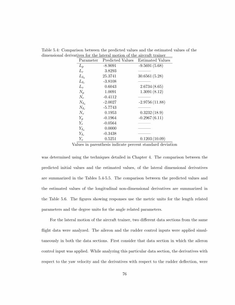
Table 5.4: Comparison between the predicted values and the estimated values of thedimensional derivatives for the lateral motion of the aircraft trainer
Parameter Predicted Values Estimated ValuesLp -8.9091 -9.5691 (5.68)Lr 3.8293 ———Lδa 25.3741 30.6561 (5.28)Lδr -3.8108 ———Lv 0.6043 2.6734 (8.65)Np 1.0091 1.3091 (8.12)Nr -0.4112 ———Nδa -2.0027 -2.9756 (11.88)Nδr -5.7743 ———Nv 0.1953 0.3232 (18.9)Yp -0.1964 -0.2967 (6.11)Yr -0.0564 ———Yδa 0.0000 ———Yδr -0.3438 ———Yv 0.5251 0.1203 (10.09)
Values in parenthesis indicate percent standard deviation
was determined using the techniques detailed in Chapter 4. The comparison between the
predicted initial values and the estimated values, of the lateral dimensional derivatives
are summarized in the Tables 5.4-5.5. The comparison between the predicted values and
the estimated values of the longitudinal non-dimensional derivatives are summarized in
the Table 5.6. The figures showing responses use the metric units for the length related
parameters and the degree units for the angle related parameters.
For the lateral motion of the aircraft trainer, two different data sections from the same
flight data were analyzed. The aileron and the rudder control inputs were applied simul-
taneously in both the data sections. First consider that data section in which the aileron
control input was applied. While analyzing this particular data section, the derivatives with
respect to the yaw velocity and the derivatives with respect to the rudder deflection, were
76

Figure 5.11: Comparison of Estimated(green) and Measured(blue) Responses for the LateralDirectional Motion of Aircraft
77
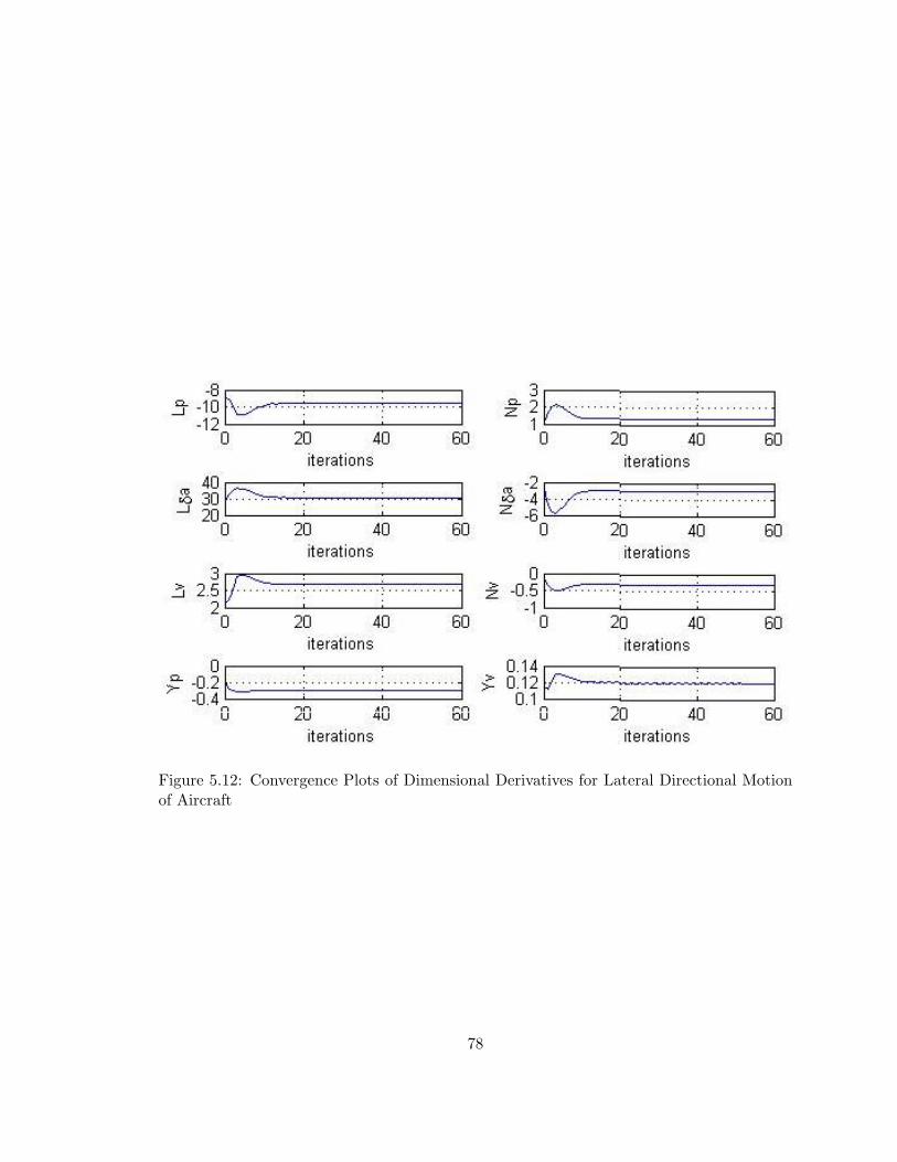
Figure 5.12: Convergence Plots of Dimensional Derivatives for Lateral Directional Motionof Aircraft
78
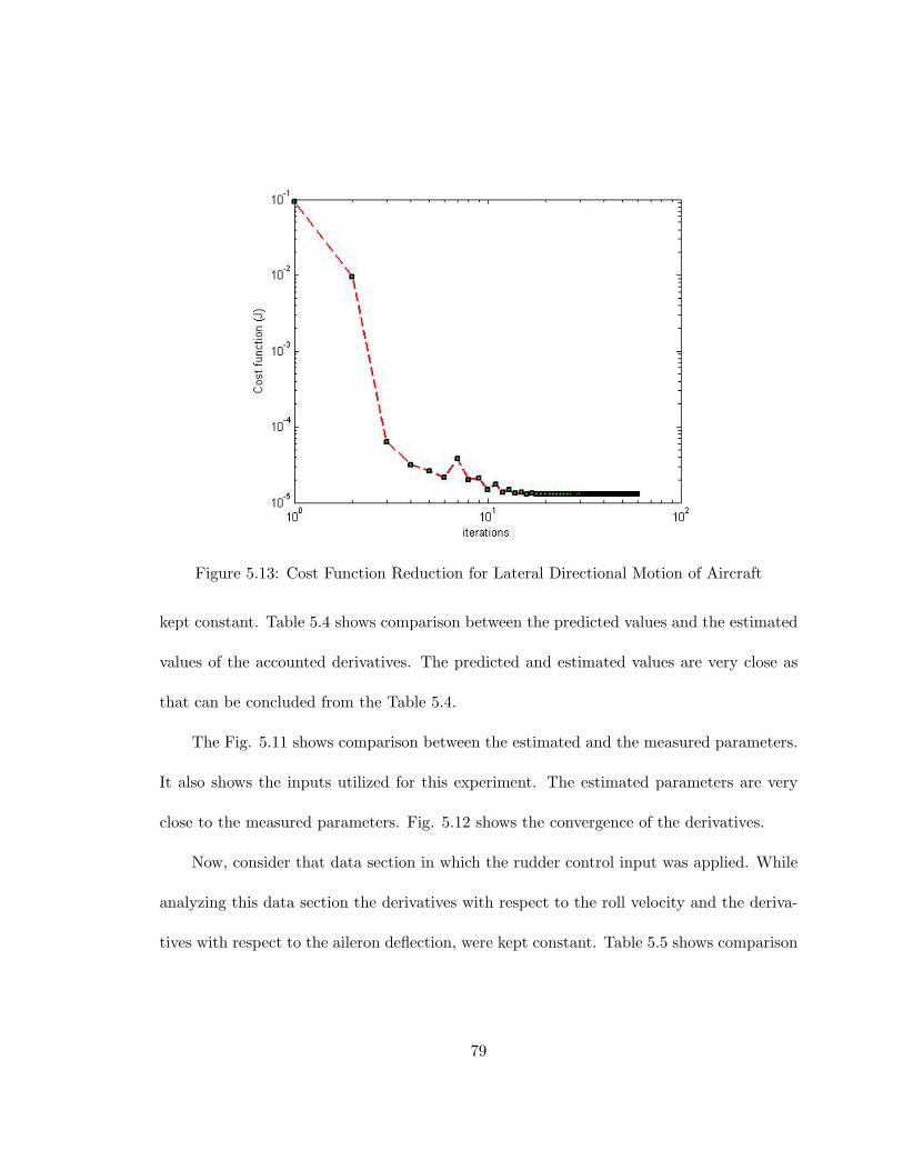
Figure 5.13: Cost Function Reduction for Lateral Directional Motion of Aircraft
kept constant. Table 5.4 shows comparison between the predicted values and the estimated
values of the accounted derivatives. The predicted and estimated values are very close as
that can be concluded from the Table 5.4.
The Fig. 5.11 shows comparison between the estimated and the measured parameters.
It also shows the inputs utilized for this experiment. The estimated parameters are very
close to the measured parameters. Fig. 5.12 shows the convergence of the derivatives.
Now, consider that data section in which the rudder control input was applied. While
analyzing this data section the derivatives with respect to the roll velocity and the deriva-
tives with respect to the aileron deflection, were kept constant. Table 5.5 shows comparison
79

Figure 5.14: Comparison of Estimated(green) and Measured(blue) Responses for the LateralDirectional Motion of Aircraft
80

Figure 5.15: Convergence Plots of Dimensional Derivatives for Lateral Directional Motionof Aircraft
81
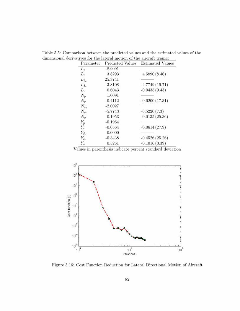
Table 5.5: Comparison between the predicted values and the estimated values of thedimensional derivatives for the lateral motion of the aircraft trainer
Parameter Predicted Values Estimated ValuesLp -8.9091 ———Lr 3.8293 4.5890 (8.46)Lδa 25.3741 ———Lδr -3.8108 -4.7749 (19.71)Lv 0.6043 -0.0435 (9.43)Np 1.0091 ———Nr -0.4112 -0.6200 (17.31)Nδa -2.0027 ———Nδr -5.7743 -6.5220 (7.3)Nv 0.1953 0.0135 (25.36)Yp -0.1964 ———Yr -0.0564 -0.0614 (27.9)Yδa 0.0000 ———Yδr -0.3438 -0.4526 (25.26)Yv 0.5251 -0.1016 (3.39)
Values in parenthesis indicate percent standard deviation
Figure 5.16: Cost Function Reduction for Lateral Directional Motion of Aircraft
82
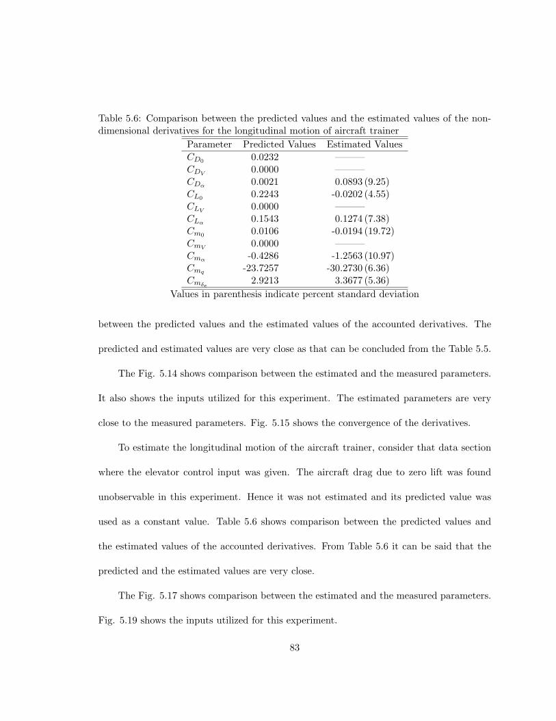
Table 5.6: Comparison between the predicted values and the estimated values of the non-dimensional derivatives for the longitudinal motion of aircraft trainer
Parameter Predicted Values Estimated ValuesCD0 0.0232 ———CDV 0.0000 ———CDα 0.0021 0.0893 (9.25)CL0 0.2243 -0.0202 (4.55)CLV 0.0000 ———CLα 0.1543 0.1274 (7.38)Cm0 0.0106 -0.0194 (19.72)CmV 0.0000 ———Cmα -0.4286 -1.2563 (10.97)Cmq -23.7257 -30.2730 (6.36)Cmδe 2.9213 3.3677 (5.36)
Values in parenthesis indicate percent standard deviation
between the predicted values and the estimated values of the accounted derivatives. The
predicted and estimated values are very close as that can be concluded from the Table 5.5.
The Fig. 5.14 shows comparison between the estimated and the measured parameters.
It also shows the inputs utilized for this experiment. The estimated parameters are very
close to the measured parameters. Fig. 5.15 shows the convergence of the derivatives.
To estimate the longitudinal motion of the aircraft trainer, consider that data section
where the elevator control input was given. The aircraft drag due to zero lift was found
unobservable in this experiment. Hence it was not estimated and its predicted value was
used as a constant value. Table 5.6 shows comparison between the predicted values and
the estimated values of the accounted derivatives. From Table 5.6 it can be said that the
predicted and the estimated values are very close.
The Fig. 5.17 shows comparison between the estimated and the measured parameters.
Fig. 5.19 shows the inputs utilized for this experiment.
83
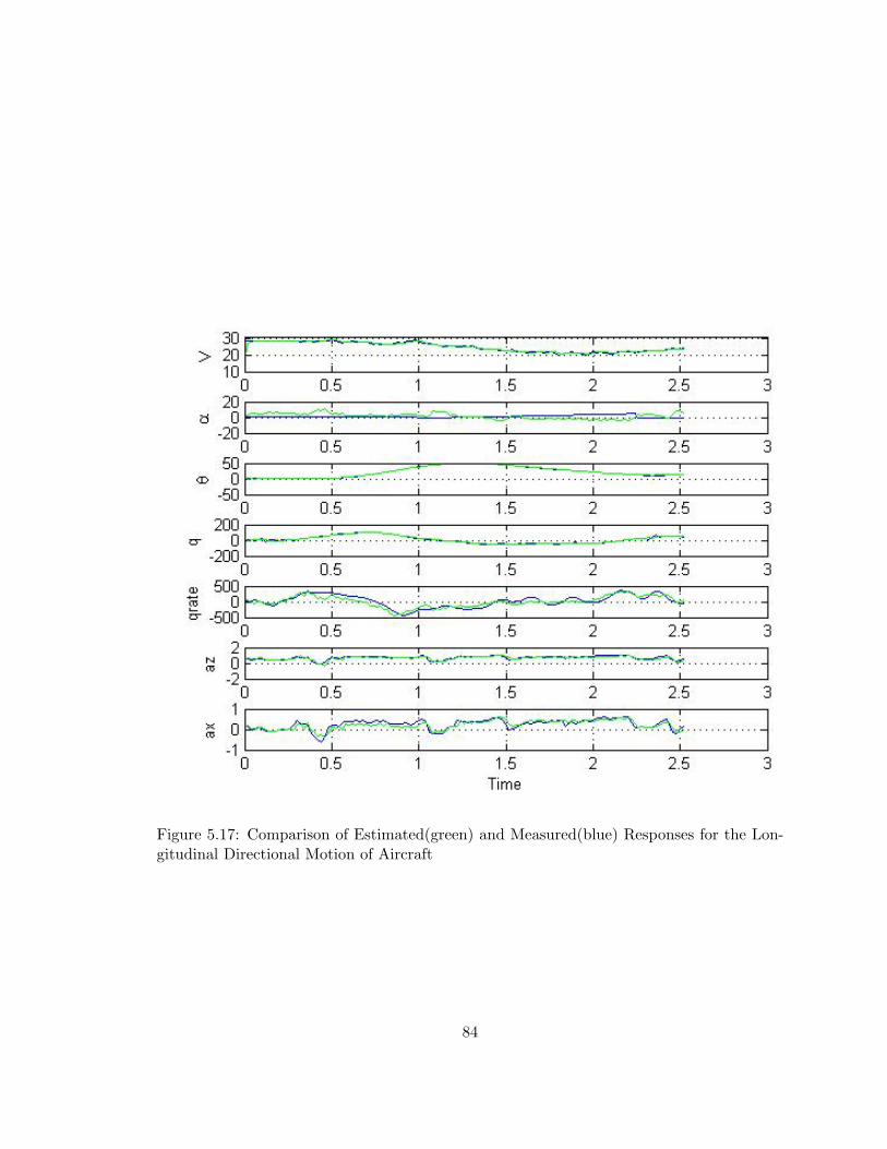
Figure 5.17: Comparison of Estimated(green) and Measured(blue) Responses for the Lon-gitudinal Directional Motion of Aircraft
84
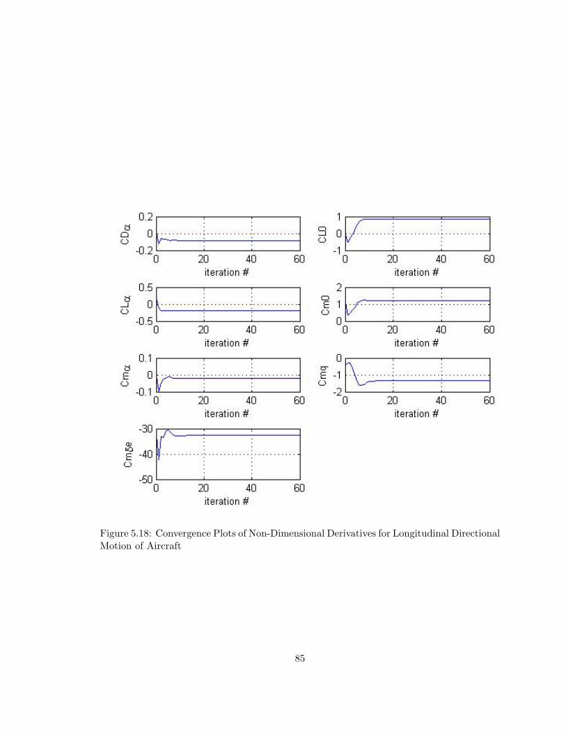
Figure 5.18: Convergence Plots of Non-Dimensional Derivatives for Longitudinal DirectionalMotion of Aircraft
85

Figure 5.19: Input for Longitudinal Motion
Figure 5.20: Cost Function Reduction for Longitudinal Motion
86
5.4 Model Validation
Model validation is the final step in the system identification process and must be
performed regardless of the accuracy of the parameter estimation techniques. The prime
reason for above statement is: estimates are not facts. The identified model must prove
that its parameters have physically acceptable values with reasonable accuracy and the best
prediction capability. Due to these arguments, the estimated parameters are compared with
the available aircraft aerodynamics data, which are obtained from wind tunnel experiments,
computational fluid dynamics or theoretical predictions. While comparing these parameters,
accuracy and precision of the estimates must be taken in to account. Model validation is
very important to gain confidence in the identified model.
87

Chapter 6
Summary
6.1 Concluding Notes
The system identification technique applied to aircraft is an efficient method for aircraft
aerodynamic modeling, based on flight test data. This thesis traced several breakthroughs
and achievements in the field of system identification, especially application to aircraft.
The thesis started with the definition, meaning and significance of system identification
and also included the necessity for it. Minimization of the maximum likelihood function
was explained in detail.
Presently, this technique involves five fundamental steps: model postulation, exper-
imental design, data analysis, parameter estimation, and model validation. All of them
were explained in detail in this thesis. The filter error technique for data analysis was dis-
cussed in detail, for both linear and nonlinear dynamical systems. Theoretical techniques
for predicting aircraft stability and control derivatives were explained in some details.
The final part of the thesis included successfully investigated examples of system iden-
tification using flight test data with results and comparison of the estimated parameters
with published data. Using the efficient results derived and presented in this thesis, and
also high quality results of many other applications published recently [92-94], a conclusion
is be made that many of the application fields which were thought as growing areas few
88
years before are now more or less, well established. The system identification methods are
now highly matured, efficient and sophisticated tools; not only for the research purposes,
but also to support and to satisfy the requirements of the aeronautical industry.
6.2 Expected Future Applications of System Identification to Aircraft
There are many interesting and necessary applications of system identification tech-
niques to aircraft which can be studied in the future. Correlation between computational
fluid dynamics (CFD) practitioners and system identification researchers should increase
considerably. In addition to the use of the system identification technique to validate the
wind tunnel and the CFD data, it should also be utilized in coordinated approaches with
the CFD, to gain advantages of the strengths of both the techniques or if one approach can
not be used efficiently somewhere, another technique can be used to fill in the gaps.
The test data of each individual parts of any aircraft can be measured using small
and inexpensive sensors. Using the modern computation capabilities, the aircraft can be
identified as distributed parameter models for the aircraft aerodynamics. Effects of each
individual sections can be considered as a results of that. This might not be an easy task, as
distributed models need more test data of each individual part, improved dynamical models
and the best wind tunnel and CFD data. The system identification researchers should
then progress towards controlled automated process and solve the particular problems if
encountered.
89
A lot of research work can be done with the nonlinear systems and unsteady aero-
dynamic models. It includes learning the basic techniques to design related experiments.
These should also ensure the necessary and critical experiments are being performed at safe
environment and at effective cost; providing the state estimates are accurate and validated
models are appropriate. System identification techniques for the nonlinear systems and un-
steady aerodynamic modeling are very complex, so the experiments need to be performed
with high accuracy and should be repeated.
For few applications, the theoretical and analytical problems will arise in the system
identification which can not be ignored. Every new flying vehicle should be tested using the
system identification techniques to validate the model. The prime practice, known as the
system identification will continue to be an important part in the aeronautical engineering,
which involves identification of the mathematical model based on the measured data from
the experiment.
90
Bibliography
[1] Jategaonkar, R. V., “Flight Vehicle System Identification: A Time Domain Methodol-ogy”, edited by Lu, F. K., Vol. 216, Progress in Aeronautics and Astronautics, AIAA,August, 2006, Reston, VA.
[2] Zadeh, L. A., “From Circuit Theory to System Theory,” Proceedings of the IRE,Vol. 50, May 1962, pp. 856-865.
[3] Anon., “He Has a Question for Any Answer,” Interview with K. Iliff by M. McCall,Antelope Valley Press, CA, Nov. 1, 1994.
[4] Jategaonkar, R. V., “Flight Vehicle System Identification - Engineering Utility,”Journal of Aircraft, Vol. 42, No. 1, 2005, pp. 11.
[5] Gauss, K. F., “Theory of the Motion of the Heavenly Bodies Moving About the Sunin Conic Section,” (Translated by Charles, H. D., 1857), Dover Publications Inc., NewYork, 1847. (Translated from Theoria Motus, 1809)
[6] Bernoulli, D., “The Most Probable Choice Between Several Discrepant Observationsand the Formation Therefrom of the Most Likely Induction,” Acta. Acad. Petrop.,1777, pp. 3-33; English Translation by Kendall, M. G., “Daniel Bernoulli on MaximumLikelihood,” Biometrika, Vol. 48, No. 1, 1961, pp. 1-18.
[7] Fisher, R. A., “On an Absolute Criterion for Fitting Frequency Curves,” Messengerof Mathematics, Vol. 41, Macmillan, London, 1912, pp. 155-160.
[8] Douglas, J., “Theorems in the Inverse Problem in the Calculus of Variations,”Proceedings of the National Academy of Science, Vol. 16, No. 3, 1940.
[9] Feldbaum, A. A., “Dual Control Theory,” Automn. Remote Control, Vol. 22, 1961,pp. 1-12 and 109-121.
[10] Cuenod, M. and Sage, A., “Comparison of Some Methods Used for Process Identifi-cation,” Automatica, Vol. 4, 1968, pp. 235-269.
[11] Balakrishnan, A. V. and Peterka, V., “Identification in Automatic Control Systems,”Automatica, Vol. 5, 1969, pp. 817-829.
[12] Astrom, K. J. and Eykhoff, P., “System Identification - A Survey,” Automatica, Vol.7, No. 2, 1971, pp. 123-162.
91
[13] Eykhoff, P., “System Identification, Parameter and State Estimation,” John Wileyand Sons, London, 1974.
[14] Kolmogorov, A. N., “Interpolation und Extrapolation von Stationaren Zufalligen Fol-gen,” Bulletin of the Academy of Sciences of the USSR Series Mathematics,Vol. 5, 1941, pp. 3-14.
[15] Wiener, N., “The Extrapolation, Interpolation and Smoothing of Stationary Time Se-ries,” OSRD 370, Report to the Services, Research Project DIC-6037, MassachusettsInst. of Technology, Cambridge, MA, Feb. 1942.
[16] Kalman, R. E., “A New Approach to Linear Filtering and Prediction Problems,”Transactions of the American Society of Mechanical Engineers, Series D, Journal ofBasic Engineering, Vol. 82, March 1960, pp. 35-45.
[17] Astrom, K. J., and Bohlin, T., “Numerical Identification of Linear Dynamic Systemsfrom Normal Operating Records,” Proceedings of the 2nd IFAC Symposium onTheory of Self − Adaptive Control Systems (England, UK), edited by Hammond,P. H., Plenum, New York, 1966, pp. 96-111.
[18] Bryan, G. H., “Stability in Aviation,” Macmillan, London, 1911.
[19] Hamel, P. G. and Jategaonkar, R. V., “Evolution of Flight Vehicle System Identifica-tion,” Journal of Aircraft, Vol. 33, No. 1, 1996, pp. 9-28.
[20] Glauert, H., “Analysis of Phugoids Obtained by a Recording Airspeed Indicator,”Aeronautical Research Council R and M 576, Jan. 1919.
[21] Norton, F. H., “The Measurement of the Damping in Roll on a JN4h in Flight,”NACA Rept. 167, 1923.
[22] Norton, F. H., “A Study of Longitudinal Dynamic Stability in Flight,” NACA Rept.170, 1923.
[23] Kroll, N., Radespiel, R., and Rossow, C., “Accurate and Efficient Flow Solvers for 3DApplications on Structured Meshes,” VKI Lecture Series 1994-05, Brussels, Belgium,March 1994.
[24] Slooff, J. W., and Schmidt, W. (eds.), “Computational Aerodynamics Based on theEuler Equations,” AG-325, AGARD, Sept. 1994.
[25] Hamel, P. G., “Determination of Aircraft Dynamic Stability and Control Parametersfrom Flight Testing,” LS-114, AGARD, May 1981 (Paper 10).
[26] “Parameter Estimation Techniques and Applications in Aircraft Flight Testing,”NASA TN-D-7647, 1974.
92
[27] “Methods for Aircraft State and Parameter Identification,” AGARD-CP-172, May1975.
[28] Breuhaus, W. O., “Summary of Dynamic Stability and Control Flight Research Con-ducted Utilizing a B-25J Airplane,” Cornell Aeronautical Lab., Buffalo, NY, Rept.TB-405-F-10, May 1948.
[29] Milliken, W. F. Jr., “Progress in Dynamic Stability and Control Research,” Journalof the Aeronautical Sciences, Vol. 14, No. 9, 1947, pp. 493-519.
[30] Milliken, W. F., Jr., “Dynamic Stability and Control Research,” Proceedings of the3rd Anglo−American Aeronautical Conference, Brighton, England, UK, 1951, pp.447-524.
[31] Seamans, R. C. Jr., Blasingame, B. P., and Clementson, G. C., “The Pulse Method forthe Determination of Aircraft Dynamic Performance,” Journal of the AeronauticalScience, Vol. 17, No. 1, Jan. 1950, pp. 22-38.
[32] Greenberg, H., “A Survev of Methods for Determining Stability Parameters of anAirplane From Dynamic Flight Measurements,” NACA TN-2340, April 1951.
[33] Shinbrot, M., “On the Analysis of Linear and Nonlinear Dynamical Systems FromTransient-Response Data,” NACA TN-3288, Dec. 1954.
[34] Howard, J., “The Determination of Lateral Stability and Control Derivatives FromFlight Data,” Canadian Aeronautics Space Journal, Vol. 13, No. 3, March 1967,pp. 126-134.
[35] Shinbrot, M., “A Least-Squares Curve Fitting Method with Applications to the Cal-culation of Stability Coefficients from Transient Response Data,” NACA TN 2341,April 1951.
[36] Wolowicz, C. H., and Holleman, E. C., “Stability Derivative Determination fromFlight Data,” Rept. 224, AGARD, Oct. 1958.
[37] Mueller, R. K., “The Graphical Solution of Stability Problems,” Journal of theAeronautical Sciences, Vol. 4, No. 8, 1937, pp. 324-331.
[38] Doetsch, K. H., “The Time Vector Method for Stability Investigations,” RoyalAircraft Establishment Rept., Aero 2495, Aug. 1953.
[39] Sternfield, L., “A Vector Method Approach to the Dynamic Lateral Stability of Air-craft,” Journal of the Aeronautical Sciences, Vol. 21, No. 4, 1954, pp. 251-256.
[40] Wolowicz, C. H., “Considerations in the Determination of Stability and ControlDerivatives and Dynamic Characteristics From Flight Data,” AGARD-AR-549, Pt.1, 1966.
93

[41] Rampy, J. M., and Berry, D. T., “Determination of Stability Derivatives From FlightTest Data by Means of High Speed Repetitive Operation Analog Matching,” FTC-TDR-64-8, Edwards, CA, May 1964.
[42] Taylor, L. W. Jr., and Iliff, K. W., “A Modified Newton-Raphson Method for Deter-mining Stability Derivatives From Flight Data,” Second International Conferenceon Computing Methods in Optimization Problems, Academic Press, New York,1969, pp. 353-364.
[43] Larson, D. B., and Fleck, J. T., “Identification of Parameters by the Method ofQuasilinearization,” Cornell Aeronautical Lab., Buffalo, New York, Rept. 164, May1968.
[44] Taylor, L. W. Jr., Iliff, K. W., and Powers, B. G., “A Comparison of Newton-Raphsonand Other Methods for Determining Stability Derivatives From Flight Data,” AIAAPaper, 69-315, March 1969.
[45] Iliff, K. W., “Aircraft Parameter Estimation” AIAA Dryden Lecture in Research for1987.
[46] Hamel, P. G., “Flight Vehicle System Identification Status and Prospects,” DFVLR-Mitt. 87-22, Nov. 1987, pp. 51-90.
[47] Grove, R. D., Bowles, R. L., and Mayhew, S. C., “A Procedure for Estimating Sta-bility and Control Parameters From Flight Test Data by Using Maximum LikelihoodMethods Employing a Real- Time Digital System,” NASA TN-D-6735, 1972.
[48] Ross, A. J., and Foster, G. W., “FORTRAN Programs for the Determination of Aero-dynamic Derivatives From Transient Longitudinal or Lateral Responses of Aircraft,”Royal Aircraft Establishment, TR-75090, Sept. 1975.
[49] Maine, R. E., and Iliff, K. W., “A FORTRAN Program for Determining AircraftStability and Control Derivatives From Flight Data,” NASA TN-D-7831, 1975.
[50] Nagy, C. J., “A New Method for Test and Analysis of Dynamic Stability and Control,”Air Force Flight Test Center, Edwards, CA, AFFTC-TD-75-4, May 1976.
[51] Mehra, R. K., “Maximum Likelihood Identification of Aircraft Parameters,”Proceedings of the Eleventh Joint Automatic Control Conference of theAmerican Automatic Control Council, Paper 18-C, Atlanta, GA, June 1970, pp.442-444.
[52] Iliff, K. W., and Maine, R. E., “Practical Aspects of Using a Maximum LikelihoodEstimatoion method to extract stability and control derivatives from flight data,”NASA TN D-8209, April 1976, pp. 1-34
94

[53] Iliff, K. W., and Maine, R. E., “Further Observations on Maximum Likelihood Esti-mates of Stability and Control Characteristics Obtained From Flight Data,” AIAAPaper 77-1133, Aug. 1977, pp. 100-112.
[54] Jategaonkar, R. V., and Plaetschke, E., “Maximum Likelihood Estimation of Param-eters in Linear Systems with Process and Measurement Noise,” DFVLR-FB 87-20,June 1987.
[55] Maine, R. E., and Iliff, K. W., “User’s Manual for MMLE3, a General FORTRAN Pro-gram for Maximum Likelihood Parameter Estimation,” NASA TP-1563, Nov. 1980.
[56] Taylor, J. S., Powell, J. D., and Mehra, R. K., “The Use of Smoothing and Other Ad-vanced Techniques for VTOL Aircraft Parameter Identification,” Final Rept., NavalAir Systems Command Contract N00019-69-C-0534, Systems Control, Inc., Palo Alto,CA, June 1970.
[57] Gerlach, O. H., “The Determination of Stability Derivatives and Performance Char-acteristics From Dynamic Maneuvers,” Delft Univ. of Technology, Dept. of AerospaceEngineering, Delft, The Netherlands, Rept. VTH-163, March 1971.
[58] Jonkers, H. L., “Application of the Kalman Filter to Flight Path Reconstruction FromFlight Test Data Including Estimation of Instrumental Bias Error Corrections,” DelftUniv. of Technology, Dept. of Aerospace Engineering, Delft, The Netherlands, Rept.VTH-162, Feb. 1976.
[59] Astrom, K. J., “Control Problems in Papermaking,” Proceedings of the IBMScientific Computing Symposium on Control Theory and Applications, IBM DataProcessing Division, White Plains, New York, 1966, pp. 135-167.
[60] Kashyap, R. L., “A New Method of Recursive Estimation in Discrete Linear Systems,”IEEE Transactions on Automatic Control, Vol. AC-15, No. 1, Feb. 1970, pp. 18-24
[61] Chen, Robert, T. N., and Eulrich, B. J., “Parameter and Model Identification ofNonlinear Dynamical Systems Using a Suboptimal Fixed-point Smoothing Algo-rithm,” Proceedings of the Twelfth Joint Automatic Control Conference of theAmerican Automatic Control Council, Paper 7-E2, Aug. 1971, pp. 731-740.
[62] Yazawa, K., “Identification of Aircraft Stability and Control Derivatives in the Pres-ence of Turbulence,” AIAA Paper 77-1134, Aug. 1977.
[63] Balakrishnan, A. V, “Stochastic System Identification Techniques,” StochasticOptimization and Control, edited by H. F. Karreman, John Wiley and sons, London,1968.
[64] Balakrishnan, A. V., “Modelling and Identification Theory: A Flight Control Appli-cation,” Theory and Applications of V ariable Structure Systems, edited by R. B.Mohler and A. Ruberti, Academic, New York, 1972.
95
[65] Iliff, K. W., “Identification and Stochastic Control with Application to Flight Controlin Turbulence,” Ph.D. Dissertation, Univ. of California, Los Angeles, CA, May 1973.
[66] Etkin, B., “Dynamics of Atmospheric Flight,” John Wiley and Sons, New York, 1972.
[67] Maine, R. E., and Iliff, K. W., “Formulation and Implementation of a Practical al-gorithm for Parameter Estimation with Process and Measurement Noise,” SIAM J.Applied Mathematics, Dec. 1981, pp. 558-579.
[68] Jategaonkar, R. V., and Plaetschket, E., “Algorithms for Aircraft Parameter Estima-tion Accounting for Process and Measurement Noise,” Journal of Aircraft, Vol. 26,No 4, April 1989, pp. 360-372.
[69] Iliff, K. W., and Taylor, L. W., “Determination of Stability Derivatives from FlightData Using a Newton-Raphson Minimization Technique,” NASA TN D-6579, March1972.
[70] Ortega, J. M., and Rheinboldt, W.C., “Iterative Solution of Nonlinear Equations inSeveral Variables,” Academic Press, New York, 1970.
[71] Balakrishnan, A. V., “Communication Theory,” 1968, McGraw-Hill, NY.
[72] Mehra, R. K., “Identification of Stochastic Linear Dynamic Systems Using KalmanFilter Representation,” AIAA Journal, Vol. 9, Jan. 1971, pp. 28-31.
[73] Gelb, A., “Applied Optimal Estimation,” The MIT Press, Cambridge, MA, 1974.
[74] Grewal, M. S., and Andrews, A. P., “Kalman Filtering Theory and Practice,” PrenticeHall, Upper Saddle River, NJ, 1993.
[75] Vaughan, D. R.,“A Non-recursive Algebraic Solution for the Discrete Riccati Equa-tion,” IEEE Transactions on Automatic Control, Vol. AC-15, Oct. 1970, pp. 597-599.
[76] Potter, J. E., “Matrix Quadratic Solutions,” SIAM Journal of AppliedMathematics, Vol. 14, May 1966, pp. 496-501.
[77] Welch, G., and Bishop, G., “An Introduction to the Kalman Filter,” SIGGRAPH,Los Angeles, CA, Aug. 2001.
[78] Maybeck, P., “Stochastic models, estimation and control,” Vol. 1, Academic Press,New York, 1979.
[79] Roskam, J., “Airplane Design Part VI: Preliminary Calculation of AerodynamicThrust and Power Characteristics”, Vol. 2, 1990, Roskam Aviation and EngineeringCorporation, Ottawa, KS.
96

[80] Roskam, J., “Airplane Flight Dynamics and Automatic Flight Controls Part I”, Vol.1, 1995, DARcorporation, Lawrence, KS.
[81] Roskam, J., “Airplane Flight Dynamics and Automatic Flight Controls Part II”, Vol.1, 1998, DARcorporation, Lawrence, KS.
[82] Raymer, D. P., “Aircraft Design: A Conceptual Approach”, Vol. 3, 1999, AIAA,Reston, VA.
[83] Nelson, R. C., “Flight Stability and Automatic Control”, Vol. 2, 1998, McGraw-Hill,NY.
[84] Plaetschke, E., Mulder, J. A., and Breeman, J. H., “Results of Beaver Aircraft Pa-rameter Identification,” DFVLR-FB 83-10, March 1983.
[85] McRuer, D., Ashkenas, I., and Graham, D., “Aircraft Dynamics and Automatic Con-trol”, Princeton Univ. Press, Princeton, NJ, 1973, pp. 292-295.
[86] Heffley, R. K., Jewell, W. F., Lehman, J. M., and Van Winkle, R. A., “A Compilationand Analysis of Helicopter Handling Qualities Data, Volume One: Data Compilation,”NASA CR-3144, Aug. 1979.
[87] Chowdhary, G. and Jategaonkar, R. V., “Aerodynamic Parameter Estimation fromFlight Data Applying Extended and Unscented Kalman Filter,” AIAA AtmosphericF light Mechanics Conference and Exhibit, Keystone, Colorado, Aug. 2006, pp.6146-6163.
[88] Jategaonkar, R. V., and Balakrishna, S., “Effects of Flap Position on Longitudi-nal Parameters of HFB-320,” TM SE-8602, NAL Bangalore, India, Feb. 1986 andDFVLR-IB 111-85/15, June 1985.
[89] Mackie, D. B., “A comparison of Parameter Estimation Results from Flight Test DataUsing Linear and Nonlinear Maximum Likelihood Methods,” DFVLR-FB 84-06, Dec.1983.
[90] Iliff, K. W., “Maximum Likelihood Estimation of Lift and Drag from Dynamic AircraftManeuvers,” Journal of Aircraft, Vol. 14, Dec. 1977, pp. 1175-1181.
[91] Hobby Outlet, 1700 S.E. Mile Hill Dr., Suite 101, Port Orchard, WA 98366.
[92] Jategaonkar, R. V., Fischenberg, D., and Gruenhagen, W., “Aerodynamic Modelingand System Identification from Flight DataRecent Applications at DLR ,” Journalof Aircraft, Vol. 41, No. 4, 2004, pp. 681-691.
[93] Wang, K. C., and Iliff, K. W., “Retrospective and Recent Examples of Aircraft Param-eter Identification at NASA Dryden Flight Research Center ,” Journal of Aircraft,Vol. 41, No. 4, 2004, pp. 752-764.
97

[94] Morelli, E. A., and Klein, V., “Application of System Identification to Aircraft atNASA Langley Research Center,” Journal of Aircraft, Vol. 42, No. 1, 2005, pp.12-25.
[95] Kuo, B. C., “Automatic Control Systems”, Prentice Hall Inc., Englewood Cliffs, NJ,1962.
[96] Hildebrand, F. B., “Introduction to Numerical Analysis”, McGraw-Hill, New York,1956, pp. 319-323.
98

Appendix A
Discretization of continuous-time state equation
A.1 Need of Discretization
The state equation utilized in the thesis is given below as [1]:
x(t) = Ax(t) +Bu(t) + bx (A.1)
This is a continuous time equation. The Kalman filter equations are discrete in nature.
Therefore, the state equation given above must be converted from a continuous-time state
equation to a discrete-time state equation. In the discrete-time case, it is assumed that the
input vector u(t) changes only at the equally spaced sampling instants. The discrete-time
state equation will be derived, which yields the exact values at t = kT , k = 0,1,2,3...N
The continuous-time state equation is Eq. A.1. Here, kT and (k+1)T are used instead
of k and (k+1)in order to clarify the analysis. The discrete-time representation of Eq. A.1
should be as follows [95]:
x(k+1)T = Θ(t)xkT + Λ(t)ukT (A.2)
The matrices Θ and Λ depend on the sampling period t. Therefore, if the period is fixed,
Θ and Λ are constant matrices.
99

A.2 Determine Θ and Λ
The general integral solution of Eq. A.1 is [95]:
x(t) = eAtx(0) + eAt∫ t
0e−AτBu(τ)dτ (A.3)
Therefore
x(k+1)T = eA(k+1)Tx(0) + eA(k+1)T∫ (k+1)T
0e−AτBu(τ)dτ (A.4)
and
xkT = eAkTx(0) + eAkT∫ kT
0e−AτBu(τ)dτ (A.5)
If Eq. A.5 is multiplied by eAT and subtracted from Eq. A.4, the following result will be
obtained [95].
x(k+1)T = eATxkT + eA(k+1)T∫ (k+1)T
kTe−AτBu(τ)dτ (A.6)
That can be simplified to [95]:
x(k+1)T = eATxkT +∫ T
0eAτBu(τ)dτ (A.7)
Comparing Eq. A.2 and Eq. A.7 [95].
Θ = eAT and Λ =∫ T
0eAτdτ (A.8)
100
Θ is termed the state transition matrix, and Λ is the integral of the state transition matrix.
Θ = eAT
Λ = A−1(eAT − I) (A.9)
where I is an identity matrix.
The final discrete-time state equation is given below:
x(tk+1) = Θx(tk) + ΛBu(tk) + Λbx (A.10)
101
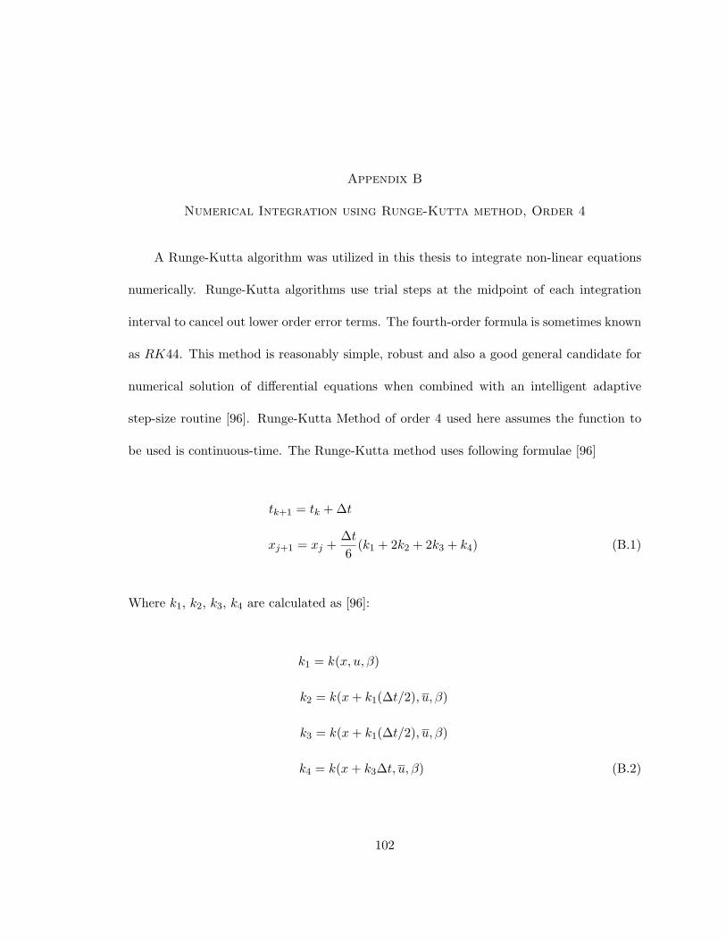
Appendix B
Numerical Integration using Runge-Kutta method, Order 4
A Runge-Kutta algorithm was utilized in this thesis to integrate non-linear equations
numerically. Runge-Kutta algorithms use trial steps at the midpoint of each integration
interval to cancel out lower order error terms. The fourth-order formula is sometimes known
as RK44. This method is reasonably simple, robust and also a good general candidate for
numerical solution of differential equations when combined with an intelligent adaptive
step-size routine [96]. Runge-Kutta Method of order 4 used here assumes the function to
be used is continuous-time. The Runge-Kutta method uses following formulae [96]
tk+1 = tk + ∆t
xj+1 = xj +∆t6
(k1 + 2k2 + 2k3 + k4) (B.1)
Where k1, k2, k3, k4 are calculated as [96]:
k1 = k(x, u, β)
k2 = k(x+ k1(∆t/2), u, β)
k3 = k(x+ k1(∆t/2), u, β)
k4 = k(x+ k3∆t, u, β) (B.2)
102


![Aviation[1]. Unusual Aircraft](https://static.fdocuments.in/doc/165x107/559393a41a28ab23348b45e0/aviation1-unusual-aircraft.jpg)