SYSTEM IDENTIFICATION OF A BRIDGE-TYPE BUILDING …
117
SYSTEM IDENTIFICATION OF A BRIDGE-TYPE BUILDING STRUCTURE A Thesis presented to the Faculty of California Polytechnic State University, San Luis Obispo In Partial Fulfillment of the Requirements for the Degree Master of Science in Architecture with a Specialization in Architectural Engineering by Pablo De La Cruz Ramos Jr. March 2013
Transcript of SYSTEM IDENTIFICATION OF A BRIDGE-TYPE BUILDING …
SYSTEM IDENTIFICATION OF A BRIDGE-TYPE
BUILDING STRUCTURE
A Thesis
presented to
the Faculty of California Polytechnic State University,
San Luis Obispo
In Partial Fulfillment
of the Requirements for the Degree
Master of Science in Architecture with a Specialization in Architectural Engineering
by
Pablo De La Cruz Ramos Jr.
March 2013

ii
© 2013
Pablo De La Cruz Ramos Jr.
ALL RIGHTS RESERVED

iii
COMMITTEE MEMBERSHIP
TITLE: System Identification of a Bridge-Type Building
Structure
AUTHOR: Pablo De La Cruz Ramos Jr.
DATE SUBMITTED: March 2013
COMMITTEE CHAIR: Dr. Graham Archer, Ph.D., P.Eng., Professor,
Architectural Engineering
COMMITTEE MEMBER: Dr. Cole McDaniel, Ph.D., P.E., Associate Professor,
Architectural Engineering
COMMITTEE MEMBER: John Lawson, M.S., S.E., Assistant Professor,
Architectural Engineering

iv
ABSTRACT
System Identification of a Bridge-Type Building Structure
Pablo De La Cruz Ramos
The Bridge House is a steel building structure located in Poly Canyon, a rural area
inside the campus of California Polytechnic State University, San Luis Obispo. The
Bridge House is a one story steel structure supported on 4 concrete piers with a lateral
force resisting system (LFRS) composed of ordinary moment frames in the N-S direction
and braced frames in the E-W direction and vertically supported by a pair of trusses. The
dynamic response of the Bridge House was investigated by means of system
identification through ambient and forced vibration testing. Interesting findings such as
diaphragm flexibility, foundation flexibility and frequency shifts due to thermal effects
were all found throughout the mode shape mapping process. Nine apparent mode shapes
were experimentally identified, N-S and E-W translational, rotational and 6 vertical
modes. A computational model was also created and refined through correlation with the
modal parameters obtained through FVTs. When compared to the experimental results,
the computational model estimated the experimentally determined building period within
8% and 10% for both N-S and E-W translational modes and within 10% for 4 of the
vertical modes.

v
ACKNOWLEDGEMENTS
I would like to thank the previous Bridge House senior project team, Brian Planas,
Megan Hanson, Dave Martin, Emma Ronney, Charles Weir, and Nick Herskedal for
converting the Bridge House into a structural dynamic laboratory, without your hard
work this thesis would not been possible. I would like to thank Ray Ward for fixing the
linear mass shaker when it was necessary. I would like to thank my brother from another
mother Sabino Tirado, thank you for traveling to Cal Poly with me and extending your
helping hand through the experimentation process. I would like to thank my mother Flora
Reyes for always giving me her love and support throughout my college education, after
9 years of college I graduated with a Master’s degree. I would like to thank my wife and
daughter Erika and Jazlene Ramos, thank you for your understanding, patience and
continuous motivation on completing this thesis. Finally, I would like to thank my
advisors Dr. Graham Archer, Dr. Cole McDaniel, and Mr. John Lawson for your
continuous help throughout the production of this thesis as this would not have been
possible without your time and expertise.

vi
Table of Contents
List of Tables .................................................................................................................... vii
List of Figures .................................................................................................................. viii
1.0 Introduction .............................................................................................................. 1
1.1 Literature Review ................................................................................................. 2
1.2 The Test Building ................................................................................................. 5
1.3 Equipment Basis ................................................................................................... 9
1.4 Mass Description ................................................................................................ 13
1.5 Stiffness Approximations of Lateral Resisting Elements .................................. 16
2.0 Experiment Basis ................................................................................................... 20
2.1 Theoretical Validation of the Experimental Readings ....................................... 20
2.2 Experimental Determination of Apparent N-S Mode Shape ............................. 24
2.2.1 Ambient Vibration Testing ......................................................................... 24
2.2.2 Forced Vibration Testing ............................................................................ 26
2.3 Experimental Determination of First E-W Mode Shape .................................... 31
2.3.1 Ambient Vibration Testing ......................................................................... 31
2.3.2 Forced Vibration Testing ............................................................................ 33
2.4 Experimental Determination of First Vertical Mode Shape............................... 37
2.4.1 Ambient Vibration Testing ......................................................................... 37
2.4.2 Forced Vibration Testing ............................................................................ 38
2.5 Modal Orthogonality of Experimental Mode Shapes ........................................ 46
2.6 Experimental Findings ....................................................................................... 51
2.6.1 Roof Diaphragm Flexibility ........................................................................ 51
2.6.2 Temperature Effects .................................................................................... 57
2.6.3 Vertical Anomaly on the Floor Diaphragm in First N-S Mode .................. 62
2.6.4 Foundation Flexibility ................................................................................. 64
3.0 Analytical Basis ..................................................................................................... 68
3.1 Progression of Analytical Modeling .................................................................. 68
3.1.1 Translational Modes.................................................................................... 69
3.1.2 Vertical Modes ............................................................................................ 79
3.2 Comparison of Analytical to Experimental Mode Shapes ................................. 80
3.3 Analytical Model of Vertical Anomaly .............................................................. 88
4.0 Conclusions ............................................................................................................ 91
4.1 AVT and FVT .................................................................................................... 91
4.1.1 Diaphragms ................................................................................................. 93
4.1.2 Foundation Flexibility ................................................................................. 94
4.1.3 Frequency Shift Due to Thermal Effects .................................................... 95
4.2 Computational Modeling.................................................................................... 96
4.2.1 Diaphragm................................................................................................... 97
4.2.2 Foundation Flexibility ................................................................................. 97
4.2.3 Comparisons of Analytical to Experimental Mode Shapes ........................ 98
5.0 References ............................................................................................................ 102
6.0 Appendix .............................................................................................................. 104

vii
List of Tables
Table 1: Mass Take-Off .................................................................................................... 13
Table 2: Stiffness Approximations of Lateral Resisting Elements ................................... 19
Table 3: Experimental vs. Computational Accelerations ................................................. 24
Table 4: Summary of Experimental Mode Shapes ........................................................... 43
Table 5 Continued: Summary of Experimental Mode Shapes........................................ 44
Table 6: Mass Weighted Correlation Numbers Comparing Experimental Mode
Shapes ............................................................................................................................... 48
Table 7: Diaphragm Stiffness and Natural Frequency of the Analytical E-W Mode
for Different Connections Types ...................................................................................... 55
Table 8: Flexible Roof Diaphragm vs. Experimental Results .......................................... 71
Table 9: Hybrid Roof Diaphragm vs. Experimental Results ............................................ 72
Table 10: Hybrid Diaphragm Model with Foundation Flexibility vs. Experimental
Results ............................................................................................................................... 76
Table 11: Flexible Roof Diaphragm Model with Diagonal Bracing vs. Experimental
Results ............................................................................................................................... 77
Table 12: Analytical Vertical Modes vs. Experimental Vertical Modes .......................... 80
Table 13: MAC Numbers Comparing Un-Swept-Apparent Results to Analytical
Results ............................................................................................................................... 83
Table 14: MAC Numbers Comparing Swept-Experimental Results
(Modes 1, 5, 2, 3, 8, 6, 4, 9, 7) to Analytical Results ....................................................... 85
Table 15: MAC Numbers Comparing Swept-Experimental Results
(Modes 1, 5, 2, 3, 8, 7, 4, 6, 9) to Analytical Results ....................................................... 87

viii
List of Figures
Figure A: Map of Vicinity .................................................................................................. 5
Figure B: Bridge House Elevation ...................................................................................... 6
Figure C: Exterior Welded Connections ............................................................................. 7
Figure D: Beam to C-Channel Connection ......................................................................... 7
Figure E: Roof and Floor Diaphragm ................................................................................. 8
Figure F: Concrete Piers ..................................................................................................... 9
Figure G: Test Setup L) Computer, Amplifier and Signal Generator, .............................. 10
Figure H: Vertical Shaker Used to Capture Vertical Modes ............................................ 11
Figure I: Accelerometer Orientation ................................................................................. 12
Figure J: Weight Verification of a 1-ft x 1-ft Square Hole on the Roof ........................... 14
Figure K: Tributary Area per Degree of Freedom for Construction of Mass Matrix ....... 15
Figure L: Mass Matrix ...................................................................................................... 16
Figure M: Approximate Soil Spring Stiffness of Actual Conditions ................................ 18
Figure N: Computational Set-up ....................................................................................... 21
Figure O: First Ambient Vibration FFT Response ........................................................... 25
Figure P: Second Ambient Vibration FFT Response ....................................................... 26
Figure Q: Forced Sweep FFT ........................................................................................... 27
Figure R: Frequency Response Curve .............................................................................. 28
Figure S: Definition of Half Power Band Method ............................................................ 29
Figure T: First Experimental N-S Mode Shape ................................................................ 30
Figure U: Ambient FFT Response .................................................................................... 31
Figure V: Ambient FFT Response .................................................................................... 32
Figure W: Forced Sweep FFT........................................................................................... 33
Figure X: Frequency Response Curve .............................................................................. 34
Figure Y: First Experimental E-W Mode Shape ............................................................... 35
Figure Z: Vertical Accelerations of the Floor and Roof Diaphragm ................................ 36
Figure AA: Ambient FFT Response ................................................................................. 38
Figure BB: Forced Sweep FFT ......................................................................................... 39
Figure CC: Frequency Response Curve ............................................................................ 40
Figure DD: First Experimental Vertical Mode Shape ...................................................... 41
Figure EE: Future Placement of Vertical Shaker to Optimize Apparent Mode 6 ............ 50
Figure FF: N-S Experimental Mode Shape ...................................................................... 51
Figure GG: E-W Apparent Mode Shape ........................................................................... 52
Figure HH: Steel Deck Panel Connections A) Seam Weld B) Button Punch C) Screw .. 53
Figure II: Roof Steel Deck Panel Configuration ............................................................... 55
Figure JJ: N-S Experimental Mode Shape ........................................................................ 57
Figure KK: Isometric on Site View of the Bridge House ................................................. 58
Figure LL: Frequency Response Shift Due to Thermal Phenomena ................................ 59
Figure MM: Surface Temperature vs. Natural Frequency ................................................ 60
Figure NN: Compression Stresses Due to Thermal Expansion ........................................ 61
Figure OO: East Elevation of First N-S Analytical Mode Shape ..................................... 61
Figure PP: Mass Normalized Vertical Floor Accelerations of the N-S Mode .................. 63
Figure QQ: Mass Normalized Translational Floor Accelerations of the N-S Mode ........ 63
ix
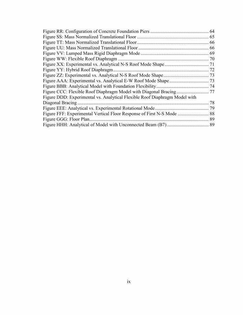
Figure RR: Configuration of Concrete Foundation Piers ................................................. 64
Figure SS: Mass Normalized Translational Floor ............................................................ 65
Figure TT: Mass Normalized Translational Floor ............................................................ 66
Figure UU: Mass Normalized Translational Floor ........................................................... 66
Figure VV: Lumped Mass Rigid Diaphragm Mode ......................................................... 69
Figure WW: Flexible Roof Diaphragm ............................................................................ 70
Figure XX: Experimental vs. Analytical N-S Roof Mode Shape ..................................... 71
Figure YY: Hybrid Roof Diaphragm ................................................................................ 72
Figure ZZ: Experimental vs. Analytical N-S Roof Mode Shape ...................................... 73
Figure AAA: Experimental vs. Analytical E-W Roof Mode Shape ................................. 73
Figure BBB: Analytical Model with Foundation Flexibility ............................................ 74
Figure CCC: Flexible Roof Diaphragm Model with Diagonal Bracing ........................... 77
Figure DDD: Experimental vs. Analytical Flexible Roof Diaphragm Model with
Diagonal Bracing .............................................................................................................. 78
Figure EEE: Analytical vs. Experimental Rotational Mode ............................................. 79
Figure FFF: Experimental Vertical Floor Response of First N-S Mode .......................... 88
Figure GGG: Floor Plan.................................................................................................... 89
Figure HHH: Analytical of Model with Unconnected Beam (B7) ................................... 89

1.0 Introduction 1
System Identification of a Bridge-Type Building Structure
1.0 INTRODUCTION
The purpose of this thesis is to capture the dynamic response of the Bridge House
through a process known as system identification. System Identification is the
development of an analytical model through its comparisons with experimentally
determined natural frequencies, mode shapes, and damping ratios.
The Bridge House, the structure investigated in this thesis is a one story steel
structure that is supported by 4 concrete piers. Its lateral force resisting system (LFRS) is
composed of ordinary moment frames in the N-S direction and braced frames in the E-W
direction. The structure is also similar to a bridge and spans 48 ft over a seasonal creek, it
is vertically supported by a pair of trusses.
To get a feel for the natural frequencies of the Bridge House in one of the N-S, E-W,
and vertical directions, ambient vibration tests (AVT) were first performed. The results of
AVT can be influenced by inconsistent noise (mainly due to wind gusts) and produce
variable results; thus, to better determine the natural frequency, AVT were followed by
forced vibration tests (FVT). Force vibration amplifies the response of the structure
through the use of a linear mass shaker with a sinusoidal output force of 30 lbs. For
translational modes the shaker was most effective when placed on the roof in its
respective direction while for vertical modes it was most effective when placed in the
vertical direction on the floor. A more precise frequency of the mode of interest was
determined by performing a micro sweep. A micro sweep was done by exciting the
structure at a small range of frequencies while simultaneously recording the steady state
accelerations. The results of the micro sweep were used to create frequency response

1.0 Introduction 2
System Identification of a Bridge-Type Building Structure
curves used to determine modal parameters such as the natural frequency and damping
ratio. Once the natural frequency was established, the shaker was then set up to
continuously oscillate at the determined natural frequency and the steady state the N-S,
E-W, and vertical accelerations were recorded. For this particular structure, accelerations
at 70 locations throughout the floor and roof were recorded, a process also known as
mode shape mapping.
An analytical model was developed to capture the dynamic behavior of the Bridge
House. The process of generating an accurate computational model required a series of
subsequent refined computational models. The analytical modeling process began with a
simple hand analysis and ended with a complex computational model. The computational
modeling was focused on the refinement of the model based on comparisons with
experimental results.
1.1 Literature Review
The Bridge House was investigated using forced vibration testing (FVT) and
exhibited a flexible roof diaphragm response in the E-W direction. Thus a literature
review was conducted on similar research topics that were performed using FVT. Other
research papers were investigated for their estimation of the flexible diaphragm stiffness
and its effect on the overall response of the structure.
In a research study that utilizes the same experimental equipment, (Jacobsen
2011) explored the behavior of two nearly identical concrete-shearwall buildings with
flexible diaphragms, one of which that had been seismically retrofitted to strengthen the
1.0 Introduction 3
System Identification of a Bridge-Type Building Structure
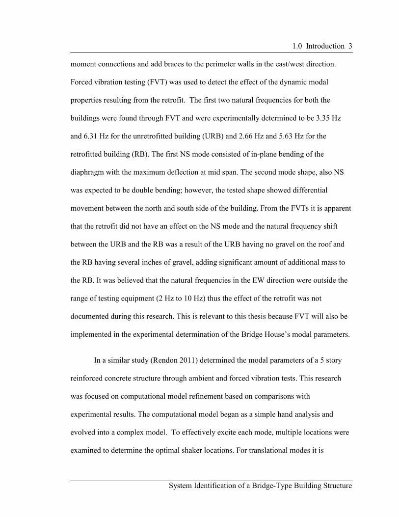
moment connections and add braces to the perimeter walls in the east/west direction.
Forced vibration testing (FVT) was used to detect the effect of the dynamic modal
properties resulting from the retrofit. The first two natural frequencies for both the
buildings were found through FVT and were experimentally determined to be 3.35 Hz
and 6.31 Hz for the unretrofitted building (URB) and 2.66 Hz and 5.63 Hz for the
retrofitted building (RB). The first NS mode consisted of in-plane bending of the
diaphragm with the maximum deflection at mid span. The second mode shape, also NS
was expected to be double bending; however, the tested shape showed differential
movement between the north and south side of the building. From the FVTs it is apparent
that the retrofit did not have an effect on the NS mode and the natural frequency shift
between the URB and the RB was a result of the URB having no gravel on the roof and
the RB having several inches of gravel, adding significant amount of additional mass to
the RB. It was believed that the natural frequencies in the EW direction were outside the
range of testing equipment (2 Hz to 10 Hz) thus the effect of the retrofit was not
documented during this research. This is relevant to this thesis because FVT will also be
implemented in the experimental determination of the Bridge House’s modal parameters.
In a similar study (Rendon 2011) determined the modal parameters of a 5 story
reinforced concrete structure through ambient and forced vibration tests. This research
was focused on computational model refinement based on comparisons with
experimental results. The computational model began as a simple hand analysis and
evolved into a complex model. To effectively excite each mode, multiple locations were
examined to determine the optimal shaker locations. For translational modes it is

1.0 Introduction 4
System Identification of a Bridge-Type Building Structure
typically ideal to excite a structure at the center of mass. However, this structure features
a large opening at the center of mass on all 5 floors, thus making it challenging to
effectively excite the structure. The first three natural frequencies recorded and their
respective modes were mapped out. The diaphragms in the 5 story structure behaved as
rigid diaphragms for the 1st 2 modes while the third mode displayed a semi rigid
diaphragm response. This is relevant to this thesis because this research highlights that
forced vibration testing can be effectively used to validate computational models.
Trembley and Stiemer (1996) investigated the dynamic behavior of low-rise steel
buildings that rely on metal roof deck diaphragm response for lateral seismic resistance.
A parametric study in the preliminary phase of the research showed that typical structures
designed according to modern building code provisions can have a fundamental period of
vibration that is much longer than that assumed in the calculations. The study also
indicated that roof diaphragm flexibility in the direction parallel to the stiff lateral frames
increases the natural period of a structure in its respective direction. This is relevant to
this thesis because the bridge house’s roof diaphragm behaves flexible in the E-W
direction whereas it is essentially rigid diaphragm in the N-S direction. As a result,
diaphragm flexibility must be accounted for when analyzing the Bridge House,
specifically in the E-W direction.
In order to calculate the natural period of a low rise steel building with a flexible
diaphragm, the stiffness of the diaphragm needs to be estimated. The stiffness of a
corrugated steel deck diaphragm is a direct indication of how the diaphragm distorts
under the influence of in-plane shear forces (Luttrell 1995). Some factors that affect

diaphragm stiffness are the geometry of the corrugated steel element and the type of side
lap connections. Corrugated steel decks have
However, when a button p
stiffness can be significantly reduced.
provided by the Steel Deck Institute Diaphragm Design Manual will be used to estimate
the diaphragm stiffness, and empirical equations derived by researchers that incorporate
diaphragm flexibility will be applied to estimate the natural period of the Bridge House.
1.2 The Test Building
The structure investigated
senior project. It is located on the northeast
University, San Luis Obispo
1.0
System Identification of a Bridge-Type Building Structure
the geometry of the corrugated steel element and the type of side
ns. Corrugated steel decks have standard geometry with minimal variation.
a button punch is alternatively used instead of seam weld,
can be significantly reduced. This is relevant to this thesis because the equations
provided by the Steel Deck Institute Diaphragm Design Manual will be used to estimate
stiffness, and empirical equations derived by researchers that incorporate
diaphragm flexibility will be applied to estimate the natural period of the Bridge House.
The Test Building
The structure investigated in this thesis was-built in 1965 by a group o
senior project. It is located on the northeast campus of the California Polytechnic State
University, San Luis Obispo. See Figure A below.
Figure A: Map of Vicinity
(Google Maps)
1.0 Introduction 5
Type Building Structure
the geometry of the corrugated steel element and the type of side
geometry with minimal variation.
instead of seam weld, the diaphragm
This is relevant to this thesis because the equations
provided by the Steel Deck Institute Diaphragm Design Manual will be used to estimate
stiffness, and empirical equations derived by researchers that incorporate
diaphragm flexibility will be applied to estimate the natural period of the Bridge House.
in 1965 by a group of students as a
California Polytechnic State

The Bridge House
construction laboratory inside
from the center of campus.
It is a one-story steel structure
composed of ordinary moment frames in the
direction. See Figure B below
The structure is similar to that of a
direction and 24-ft in the transverse direction
trusses along the longitudinal direction
large glass windows and plywood sh
replacement for windows that were broken as a result of vandalism.
The columns and braces on the exterior of the building are
sections (HSS3X3X1/4) that are
channels are also the chord members of the truss s
1.0
System Identification of a Bridge-Type Building Structure
Bridge House is located in a remote area known as the outdoor experimental
construction laboratory inside of Poly Canyon and it is approximately 1.2 miles away
from the center of campus.
story steel structure with a lateral force resisting system (LFRS)
rdinary moment frames in the N-S direction and braced frame
below.
Figure B: Bridge House Elevation
(Nelson)
is similar to that of a bridge and spans 48-ft in the longitudinal
ft in the transverse direction. It is vertically supported by a
along the longitudinal direction. The façade of the building is a combination of
large glass windows and plywood sheathing. The plywood sheathing is a temporary
replacement for windows that were broken as a result of vandalism.
The columns and braces on the exterior of the building are hollow structural
) that are welded in between two c-channels (C12X20.7)
hannels are also the chord members of the truss system. See Figure C below.
1.0 Introduction 6
Type Building Structure
the outdoor experimental
t is approximately 1.2 miles away
rce resisting system (LFRS)
and braced frames in the E-W
ft in the longitudinal
t is vertically supported by a pair of
ilding is a combination of
eathing. The plywood sheathing is a temporary
hollow structural
C12X20.7). The c-
below.

1.0 Introduction 7
System Identification of a Bridge-Type Building Structure
Figure C: Exterior Welded Connections
The corner columns of the building are built up sections composed of (4)
HSS3X3X1/4 tubes as seen in the Figure C above. Only three HSS tubes can be seen in
Figure C; the fourth tube lies underneath the inside c-channel. A typical weld connection
for a brace or column to the truss chord consists of four 12-inch-long fillet welds, one for
each corner of the HSS.
The interior roof and floor beams are wide flange sections spaced at 8 ft on center
and are connected to the web of the truss chords via steel tabs. See Figure D below.
Figure D: Beam to C-Channel Connection
The steel tabs are located on both sides of the beam web and are connected with
fillet welds.

1.0 Introduction 8
System Identification of a Bridge-Type Building Structure
The roof diaphragm is made up of rigid insulation topped with gravel-on-metal
deck, while the floor diaphragm is composed of 3 ½- inch thick lightweight concrete also
supported by metal deck. See Figure E below.
Figure E: Roof and Floor Diaphragm
The metal decks spans 8-ft and as common practice, it is reasonable to assume
that the roof deck panels and roof beams are interconnected through intermediate spot
welds. In the original senior project report of 1965, the floor beams were designed non
composite (Bridge House, 1966); thus, the connections between the floor diaphragm and
floor beams are also assumed to be intermediate spot welds.
The building rests on four 18-inch x 18-inch concrete piers, one for each corner of
the building. See Figure F below.

1.0 Introduction 9
System Identification of a Bridge-Type Building Structure
Figure F: Concrete Piers
The embedment and exposure of each pier differs at each corner. It is assumed
(verified through experimental testing) that the floor diaphragm is pin connected to the
concrete piers via embed plates, rebar, and fillet welds. A soils report is not available to
determine the current site conditions; however, the soil contains some cohesion with
granular material; therefore the soil is in the range of clayey sand.
1.3 Equipment Basis
Forced Vibration Testing (FVT) (McDaniel and Archer 2010) was used in this
thesis to experimentally determine the natural frequencies and mode shapes of the Bridge
House. To document the resonant frequencies and mode shapes, the following equipment
was used:
• Accelerometers
• Data Acquisition (DAQ)
• Dell Computer with Lab View Software
• Electronic Signal Generator

1.0 Introduction 10
System Identification of a Bridge-Type Building Structure
• Amplifier
• Linear Mass Shaker
This equipment can also be seen in Figure G below.
Figure G: Test Setup L) Computer, Amplifier and Signal Generator,
TR) Accelerometers, BR) Linear Mass Shaker
The linear mass shaker is an 80-lb machine that oscillates at various frequencies
and amplitudes that can generate a sinusoidal force up to 30 lbs. Generally friction
between the base of the shaker and the floor is sufficient to transfer the force generated
from the shaker onto the structure, thus no additional anchoring devices are needed.
Designed for scale structures, the linear shaker, when properly placed, has been proven to
excite buildings under 4 floors, and under 30,000 square feet (McDaniel and Archer
2010). The same linear shaker was used to excite the Bridge House, a structure that is far
within the limitations of the equipment, as it is a 1-story steel structure with a square
footage of 1,152 sq-ft. and an approximate weight of 41tons.
In 2011 the Bridge House was renovated and converted into a structural dynamics
laboratory (Rehabilitation, 2011). The senior project team fabricated shaker mounts at
1.0 Introduction 11
System Identification of a Bridge-Type Building Structure
the roof level to easily hoist and fasten the linear mass shaker to the roof. The Bridge
House is a 1-story structure, thus exciting the structure at the roof ideally maximizes
response of the first translational modes. The linear mass shaker fastened to the roof can
also be seen in the test setup depicted in Figure G on page 10.
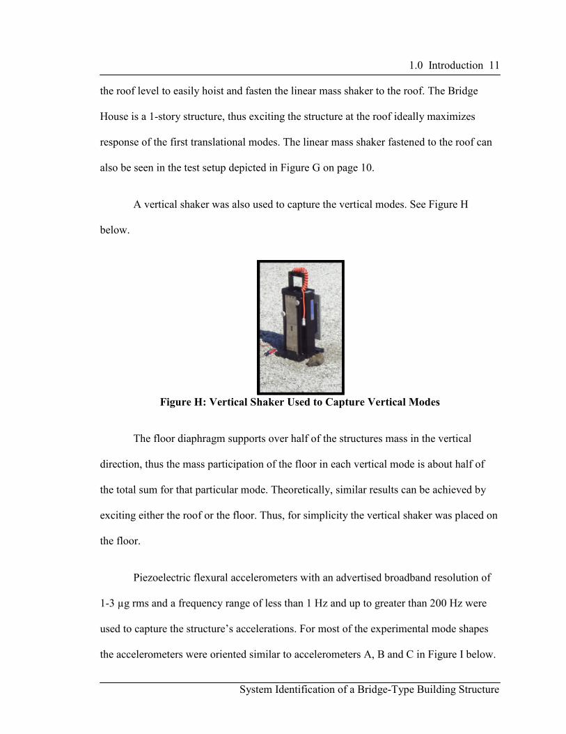
A vertical shaker was also used to capture the vertical modes. See Figure H
below.
Figure H: Vertical Shaker Used to Capture Vertical Modes
The floor diaphragm supports over half of the structures mass in the vertical
direction, thus the mass participation of the floor in each vertical mode is about half of
the total sum for that particular mode. Theoretically, similar results can be achieved by
exciting either the roof or the floor. Thus, for simplicity the vertical shaker was placed on
the floor.
Piezoelectric flexural accelerometers with an advertised broadband resolution of
1-3 µg rms and a frequency range of less than 1 Hz and up to greater than 200 Hz were
used to capture the structure’s accelerations. For most of the experimental mode shapes
the accelerometers were oriented similar to accelerometers A, B and C in Figure I below.

1.0 Introduction 12
System Identification of a Bridge-Type Building Structure
The 3 accelerometers were mounted to a steel plate, one for each direction along the X, Y
and Z coordinates.
An additional accelerometer was introduced to capture the rotational mode of
vibration about the vertical axis. Accelerometer D as in Figure I below was set 48-ft
away from accelerometer A and the rotation was calculated using equation 1 below.
gx
BA ×− , Equation 1
Where A and B are the accelerations from the two accelerometers (g),
g is the acceleration due to gravity (ft/sec2), and
x is the distance between accelerometers A and B (ft).
Figure I: Accelerometer Orientation
A 24-bit analog to digital converter was used to process the signals from the
accelerometers. These signals were processed further using the standard lab software,
LabView (McDaniel and Archer 2010). The software was set up to scale the readings
from each accelerometer and provide a time history of the accelerometer readings as well
as perform a Fast Fourier Transform (FFT) of the data to provide frequency information.
(Rendon, 2011)

1.0 Introduction 13
System Identification of a Bridge-Type Building Structure
1.4 Mass Description
The Bridge House is a small structure with a 48-ft x 24-ft footprint and an
approximate weight of 41 tons. Table 1 below illustrates the mass take off of the different
structural and nonstructural components of the building that contribute to the mass.
Table 1: Mass Take-Off
Roof
Structural
Metal Deck 18-gauge steel 3.0 psf
Framing W8x31 @ 8ft o.c. 4.5 psf
Framing C12x20.7 5.2 psf
Columns HSS3x3x.25 1.1 psf
Braces HSS3x3x.25 1.0 psf
Nonstructural
Roofing Rigid Insulation and Gravel 15.0 psf
Total 29.8 psf
Floor
Structural
Concrete 4" thick lightweight conc 22.5 psf
Metal Deck 18-gauge steel 3.0 psf
Framing W8x35 @ 8ft o.c. 5.1 psf
Framing C12x20.7 5.2 psf
Columns HSS3x3x.25 1.1 psf
Braces HSS3x3x.25 1.0 psf
Nonstructural
Window/Door Frames L3x2x1/4 1.2 psf
L3x2x1/5 1.0 psf
Facades Plywood1
0.4 psf
Glass1
0.8 psf
Other Misc 0.2 psf
Total 41.5 psf
1 The façade of The Bridge House is composed of plywood and glass. These values
represent the total weight of the material divided by the square footage of the floor.

1.0 Introduction 14
System Identification of a Bridge-Type Building Structure
Nonstructural components such as utility equipment and furnishings usually
contribute a substantial amount of additional mass to a structure; however, due to the
current vacant occupancy of the structure, the nonstructural components only make up
about 20% of the total mass.
Current roofing manufacturers list gravel and rigid foam insulation at a material
weight of approximately 7 psf and 1.5 psf, respectively. However, due to the relatively
small size of the structure, small change in mass can result in considerable change in the
modal parameters. Therefore, the weight of the roof had to be verified.
To verify the weight of the roof, a 1-ft x 1-ft square of gravel and rigid foam
insulation was cut out, placed into a bag, and weighed as in Figure J below.
Figure J: Weight Verification of a 1-ft x 1-ft Square Hole on the Roof
The 1-ft x 1-ft square of gravel and rigid insulation weighed 15 lbs, equivalent to
15 psf, exceeding the maximum listed weight by 214 percent.
The façade of the structure rests on the on top of the floor slab and is connected
with seldom welds to the columns without any evident connections to the roof; hence any
weight associated with the façade is resisted by the floor. This assumption is essential
1.0 Introduction 15
System Identification of a Bridge-Type Building Structure
when creating the mass matrix since it contributes additional weight to the perimeter of
the floor diaphragm.
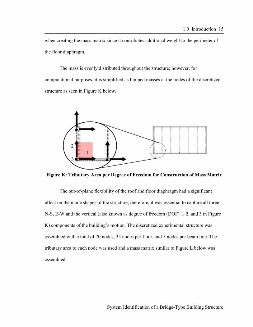
The mass is evenly distributed throughout the structure; however, for
computational purposes, it is simplified as lumped masses at the nodes of the discretized
structure as seen in Figure K below.
Figure K: Tributary Area per Degree of Freedom for Construction of Mass Matrix
The out-of-plane flexibility of the roof and floor diaphragm had a significant
effect on the mode shapes of the structure; therefore, it was essential to capture all three
N-S, E-W and the vertical (also known as degree of freedom (DOF) 1, 2, and 3 in Figure
K) components of the building’s motion. The discretized experimental structure was
assembled with a total of 70 nodes, 35 nodes per floor, and 5 nodes per beam line. The
tributary area to each node was used and a mass matrix similar to Figure L below was
assembled.

1.0 Introduction 16
System Identification of a Bridge-Type Building Structure
Figure L: Mass Matrix
The lumped mass at each node is the sum of the mass contributions of all the
structural elements tributary to the node and corresponds to all translational DOF at that
node (e.g., M11 = M1 is corresponds to DOF 1 and Mij is corresponds to DOF i where i=j).
In general, for a lumped mass model, the diagonal entries in the mass matrix such as Mij
are equal to 0 when i≠ j.
1.5 Stiffness Approximations of Lateral Resisting Elements
In addition to the mass matrix, the lateral stiffness of the structure was
approximated to hand calculate the theoretical natural frequencies and mode shapes. For
purposes of calculating the stiffness of the LFRS, it was assumed that the structure has a
rigid diaphragm in both directions; therefore, only the stiffness of the LFRS was
necessary. The stiffness in the N-S direction is provided by all perimeter columns in
which the corner columns are built up sections composed of (4) HSS3X3X1/4 and the
intermediate columns are single HSS3X3X1/4. The stiffness in the N-S direction was
approximated using equation 2.
∑=−3
12
L
EIk SN
Equation 2

1.0 Introduction 17
System Identification of a Bridge-Type Building Structure
Where L is the length of the column and
EI is bending stiffness of the column.
The stiffness in the E-W direction is provided by the HSS3X3X1/4 diagonal
braces. There are 6 diagonal braces on each north and south face of the structure;
however, because compression braces provide minimal stiffness, only the tension braces
were considered when calculating the stiffness in the E-W direction. The stiffness in the
E-W direction was approximated using equation 3 below.
θ2COS
L
EAk WE ∑=− , Equation 3
Where L is the length of the diagonal brace,
EA is the axial stiffness of the diagonal brace, and
θ is the angle between diagonal brace and horizontal plane.
The lateral stiffness of the concrete piers was not necessary for the hand
calculations; however, it will be referenced at a later section in this thesis. Assuming
similar behavior as a cantilevered beam, the lateral stiffness of the concrete piers was
approximated using equation 4 below.
3.
3
L
EIk cracked
PierConc = Equation 4
Where L is the average length of the concrete pier and
crackedEI is the cracked bending stiffness of the concrete pier
Icracked was chosen in lieu of Igross based a conservative assumption assuming the
lateral stiffness provided by the soil is significantly less than the lateral stiffness of the
1.0 Introduction 18
System Identification of a Bridge-Type Building Structure
concrete piers. The concrete piers are embedded into the soil and in order to preserve the
existing conditions of the Bridge House, the concrete pier lengths could not be verified.
As an alternative, as-built construction drawings generated by the 1966 senior project
Bridge House team were used as reference (see Appendix on page 104).
In addition to the stiffness generated by the concrete piers, there is also lateral
stiffness provided by the soil. A soils report is not available to determine the current site
conditions; however, the soil contains some cohesion with granular material; therefore
the soil is in the range of clayey sand. A range of typical values for the modulus of
subgrade reaction for clayey, medium-dense sand is given in the textbook Foundation
Analysis and Design (Bowles 1996). The soil’s modulus of sub grade reaction is a
function of soil compaction and soil moisture content and can range anywhere from 61
k/ft3 to 573 k/ft
3.
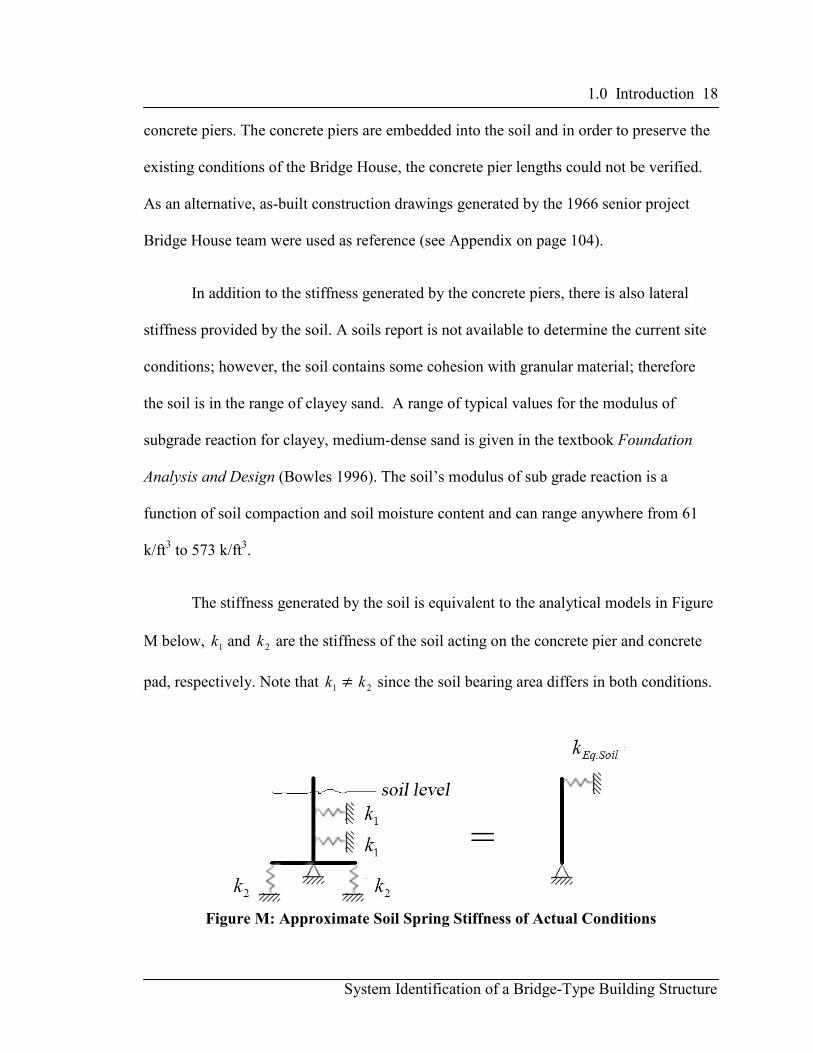
The stiffness generated by the soil is equivalent to the analytical models in Figure
M below, 1k and 2k are the stiffness of the soil acting on the concrete pier and concrete
pad, respectively. Note that 1k ≠ 2k since the soil bearing area differs in both conditions.
Figure M: Approximate Soil Spring Stiffness of Actual Conditions

1.0 Introduction 19
System Identification of a Bridge-Type Building Structure
To simplify 1k and 2k an equivalent analytical model was used where SoilEqk . was
calculated using equation 5 below. Equation 5 was derived by applying a unit rotation at
the base of the analytical model in Figure M and subsequently using the fundamental
statics approach of∑ � = 0.
2
3
2
3
.12
1''
6
1
h
bkd
h
kbhk SS
SoilEq ⋅+⋅= Equation 5
Where SoilEqk . is the equivalent soil spring stiffness in the analytical model,
h is the average height of the pier,
b is the depth and width of the concrete pad,
Sk is the modulus of subgrade reaction,
'h is the effective soil height,
'b is the depth and width of concrete pier.
Equation 5 determined that the minimum and maximum soil spring stiffness
based on the previously defined range for the modulus subgrade reaction, 7 k/in and 65
k/in, respectively. Thus the total soil stiffness in each direction varied from 28 k/in to 260
k/in (4 piers).
Table 2 below is a summary of all the previously calculated stiffness values.
Table 2: Stiffness Approximations of Lateral Resisting Elements
SNk − WEk − Σ PierConck . SoilEqk .
87 k/in 1149 k/in 576 k/in 7 k/in – 65 k/in

2.0 Experiment Basis 20
System Identification of a Bridge-Type Building Structure
2.0 EXPERIMENT BASIS
One of the goals of this thesis was to determine the natural frequencies and mode
shapes of the Bridge House. Obtaining the first 2 translational and the first rotational
mode shapes was the primary objective, while all other vertical modes were secondary.
To effectively excite the first N-S and E-W translational modes, the linear mass shaker
was placed on the roof. The floor diaphragm supports slightly over half of the structure’s
mass in the vertical direction, thus the mass participation of the floor for each vertical
mode is about half of the total sum in each vertical mode. Thus it was appropriate to
excite the structure in the vertical direction by placing the shaker on the floor.
2.1 Theoretical Validation of the Experimental Readings
To validate the experimental results, a simplified theoretical forced vibration modal
analysis using the principle of dynamic amplification was performed. Dynamic
amplification utilizes amplification factors that are used to amplify the response of the
structure’s steady state accelerations under harmonic loading at its respective natural
frequency. For this analysis, the roof diaphragm was assumed to be rigid in both
translational directions, and the 30-lb harmonic force was applied to the roof’s center of
mass at a frequency of 4.45 Hz as shown in Figure N below.

2.0 Experiment Basis 21
System Identification of a Bridge-Type Building Structure
Figure N: Computational Set-up
The equation of motion of a harmonic forced vibration response is given in
equation 6 (Chopra 2007):
tpkuucum o ωsin=++ &&& Equation 6
Where op is the amplitude of the force,
ω is the exciting frequency,
m is the mass of the system,
k is the stiffness of the system,
c is the damping constant, u is the displacement of the system,
u& is the velocity of the system, and
u&& is the acceleration of the system.
The complementary solution to the differential equation in equation 6 is given in
equation 7:
( ) ( ) tDtCtBtAetu DD
tn ωωωωξωcossinsincos +++= −
Equation 7
Where ξ is the damping ratio (experimentally determined),
nω is the natural frequency of the system,
Dω is given by Equation 8, and
2.0 Experiment Basis 22
System Identification of a Bridge-Type Building Structure
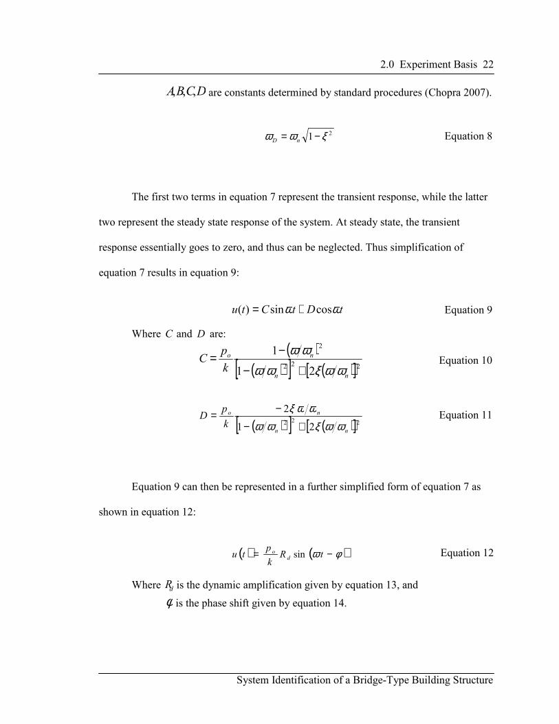
DCBA ,,, are constants determined by standard procedures (Chopra 2007).
21 ξωω −= nD
Equation 8
The first two terms in equation 7 represent the transient response, while the latter
two represent the steady state response of the system. At steady state, the transient
response essentially goes to zero, and thus can be neglected. Thus simplification of
equation 7 results in equation 9:
tDtCtu ωω cossin)( += Equation 9
Where C and D are:
( )( )[ ] ( )[ ]222
2
21
1
nn
no
k
pC
ωωξωωωω
+−
−= Equation 10
( )[ ] ( )[ ]22221
2
nn
no
k
pD
ωωξωωωωξ
+−
−= Equation 11
Equation 9 can then be represented in a further simplified form of equation 7 as
shown in equation 12:
( ) ( )φω −= tRk
ptu d
o sin Equation 12
Where dR is the dynamic amplification given by equation 13, and
φ is the phase shift given by equation 14.

2.0 Experiment Basis 23
System Identification of a Bridge-Type Building Structure
( )[ ] ( )[ ]222
21
1
nn
dR
ωωξωω +−= Equation 13
( )( )2
1
1
2tan
n
n
ωωωωξφ
−= −
Equation 14
Equation 12 defines the displacement of a single degree of freedom with respect
to time under a harmonic load, which is also equivalent to the modal displacement
(equation 15) of a single degree of freedom (DOF) in a multi DOF system.
( ) ( )φω −= tRk
ptq d
o sin Equation 15
Differentiating equation 15 twice yields equation 16, the modal accelerations:
( ) ( )nd
n
nn tR
k
ptq φωω −−= sin2
&& Equation 16
Where )(tqn&&
is the acceleration of the nth mode,
nk is equal to
2
nω when mode shapes are mass orthonormalized, and
np is the effect of the loading on mode n, given in equation 17:
pp T
nn φ= Equation 17
The modal accelerations are then recoupled into the equation of motion by using
equation 18:
( ) qtu Φ=&& Equation 18

2.0 Experiment Basis 24
System Identification of a Bridge-Type Building Structure
Where ( )tu&& are the global acceleration, and
Φ is the matrix of mode shapes.
Using the mass in Table 1 on page 13 and the lateral stiffness in the N-S and E-W
direction, the results of Eq. 19 using are summarized in Table 3 below and compared to
the experimental accelerations for nωω = and ξ = 0.044 (experimentally determined).
The mass and stiffness matrices along with the theoretical results are in the appendix.
Table 3: Experimental vs. Computational Accelerations
Computational Accelerations Experimental Accelerations Percent Difference
Uy 5.23 m g 5.90 m g 11.4 %
The computational accelerations were 11.4% different from the experimental
accelerations.
2.2 Experimental Determination of Apparent N-S Mode Shape
The N-S mode was experimentally determined using ambient vibration and forced
vibration tests, the mode was anticipated to be a translational dominated mode in the N-S
direction.
2.2.1 Ambient Vibration Testing
Ambient vibration testing (AVT) was first performed to try to determine the
approximate frequency at which the first mode of vibration in the N-S direction occurred.
AVT was performed without the linear mass shaker and due to the unoccupied state of

2.0 Experiment Basis 25
System Identification of a Bridge-Type Building Structure
the Bridge House; its main source for AVT was wind. To get a good representation of the
natural frequencies, an average of 10 thirty-second AVT’s were used to create a FFT
response curve such as Figure O below. A peak in the FFT response curve represents a
possible mode.
Figure O: First Ambient Vibration FFT Response
The accelerometers were placed in a strategic way in an attempt to locate the
frequency at which the response of the mode is maximized. It was predicted that the first
N-S mode was primarily uniform N-S translational motion at the roof, thus the placement
of the accelerometers at any location within the roof diaphragm was appropriate.
The first AVT was performed with two accelerometers at the south face of the
structure on the roof (see Figure O). The FFT response curve in Figure O illustrates a
distinct peak in the N-S direction at about 5 Hz, where the response in the E-W direction
was negligible. This was a good indication that the N-S mode was about 5 Hz. An

2.0 Experiment Basis 26
System Identification of a Bridge-Type Building Structure
additional AVT at another distinct location on the roof was used to help verify that the
peak at about 5 Hz was dominated by N-S motion, see Figure P below.
Figure P: Second Ambient Vibration FFT Response
The results of the second AVT also indicated a strong ambient response in the N-
S direction at about 5 Hz. The E-W response was negligible at about 5 Hz; however,
there appeared to be an E-W peak at about 10 Hz, possibly the first E-W mode.
Subsequently, forced vibration testing (FVT) was performed to overcome the ambient
response of the structure and more accurately determine the natural frequency of the N-S
mode.
2.2.2 Forced Vibration Testing
Following AVT, FVT was performed in an attempt to amplify the response of the
structure to isolate the N-S mode. The linear mass shaker was placed at the center of
mass on the roof where the forced vibration sweep was executed for a range of

2.0 Experiment Basis 27
System Identification of a Bridge-Type Building Structure
frequencies of 3-6 Hz. The results of the forced vibration sweep can be seen in the FFT
in Figure Q below.
Figure Q: Forced Sweep FFT
At about 5 Hz, it is clear that the response is dominated by N-S motion, thus
reinforcing that the N-S mode is at approximately 5 Hz. Note that the peak acceleration
in the forced vibration sweep shown in Figure Q is 167 times greater than the peak
acceleration in the AVT.
To better determine the frequency at which the N-S mode occurred, a micro
sweep was subsequently performed. A micro sweep was done by exciting the structure
through a small range of frequencies while simultaneously recording the steady state
accelerations. The shaker was placed in the same location and orientated in the same
direction as in Figure Q as it was evident that the N-S motion was maximized while the
E-W minimized. Figure R below are results of the micro sweep for the N-S mode, also
known as the N-S mode frequency response curve.

2.0 Experiment Basis 28
System Identification of a Bridge-Type Building Structure
Figure R: Frequency Response Curve
The roof experienced a peak acceleration of about 5 m g at a frequency of 4.45
Hz. Note that the accelerations measured in the frequency response curve were steady
state; thus, are 1667 times larger than the recorded ambient accelerations. The results of
the AVT and FVT illustrate that as the accelerations demands increased (from AVT to
FVT), the natural frequency slightly decreased. This occurs from the slippage in the
connections as the acceleration demands increase, slightly reducing the stiffness. The
effective damping shown in Figure R was calculated utilizing the half power band
method as in Figure S below.
2.0 Experiment Basis 29
System Identification of a Bridge-Type Building Structure
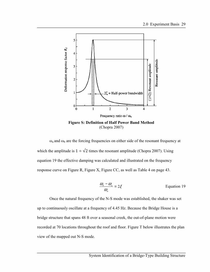
Figure S: Definition of Half Power Band Method
(Chopra 2007)
ωa and ωb are the forcing frequencies on either side of the resonant frequency at
which the amplitude is 1 ÷ √2 times the resonant amplitude (Chopra 2007). Using
equation 19 the effective damping was calculated and illustrated on the frequency
response curve on Figure R, Figure X, Figure CC, as well as Table 4 on page 43.
ξω
ωω2=
−
n
ab Equation 19
Once the natural frequency of the N-S mode was established, the shaker was set
up to continuously oscillate at a frequency of 4.45 Hz. Because the Bridge House is a
bridge structure that spans 48 ft over a seasonal creek, the out-of-plane motion were
recorded at 70 locations throughout the roof and floor. Figure T below illustrates the plan
view of the mapped out N-S mode.
2.0 Experiment Basis 30
System Identification of a Bridge-Type Building Structure
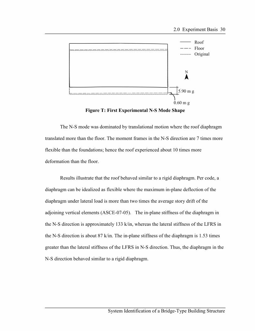
Figure T: First Experimental N-S Mode Shape
The N-S mode was dominated by translational motion where the roof diaphragm
translated more than the floor. The moment frames in the N-S direction are 7 times more
flexible than the foundations; hence the roof experienced about 10 times more
deformation than the floor.
Results illustrate that the roof behaved similar to a rigid diaphragm. Per code, a
diaphragm can be idealized as flexible where the maximum in-plane deflection of the
diaphragm under lateral load is more than two times the average story drift of the
adjoining vertical elements (ASCE-07-05). The in-plane stiffness of the diaphragm in
the N-S direction is approximately 133 k/in, whereas the lateral stiffness of the LFRS in
the N-S direction is about 87 k/in. The in-plane stiffness of the diaphragm is 1.53 times
greater than the lateral stiffness of the LFRS in N-S direction. Thus, the diaphragm in the
N-S direction behaved similar to a rigid diaphragm.
2.0 Experiment Basis 31
System Identification of a Bridge-Type Building Structure
2.3 Experimental Determination of First E-W Mode Shape
The E-W mode was experimentally determined using ambient vibration and forced
vibration tests, the mode was anticipated to be a translational dominated mode in the E-W
direction.
2.3.1 Ambient Vibration Testing
The subsequent target mode shape was the E-W mode. As previously mentioned
in section 2.2.1, the accelerometers were placed in a strategic way to locate the frequency
at which the primary response of the particular mode shape was maximized.
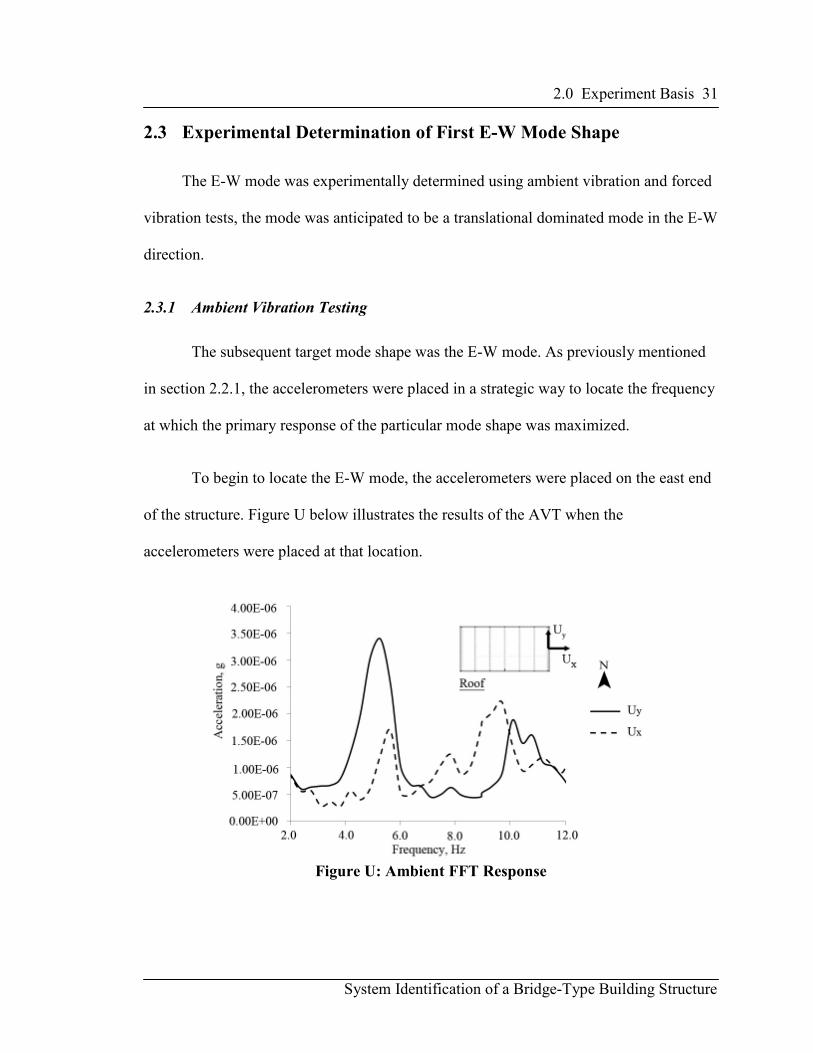
To begin to locate the E-W mode, the accelerometers were placed on the east end
of the structure. Figure U below illustrates the results of the AVT when the
accelerometers were placed at that location.
Figure U: Ambient FFT Response

2.0 Experiment Basis 32
System Identification of a Bridge-Type Building Structure
Multiple peaks occur in the ambient FFT response curves in Figure U. Similar to
previous AVT’s, the vertical ambient response was again greater than both the N-S and
E-W by order of magnitudes, thus, to better examine the N-S and E-W response, the
vertical response was omitted from Figure U. Figure U indicates that the ambient
response in the E-W direction was strongest at 9 Hz; however, other peaks in the E-W
direction are also in existence and need to be considered. For a closer look at the overall
ambient response of the structure, Figure V below was included to examine the vertical
ambient response along with the N-S and E-W response.
Figure V: Ambient FFT Response
It is clear in Figure V that the majority of the peaks that correspond to the E-W
response are located below the vertical response peaks. The vertical response was
significantly greater than the E-W response, indicating that these peaks are most likely a
vertical mode. However if the E-W response is closely examined at slightly less than 10
Hz, it is evident that there are 2 peaks that are closely spaced. The second peak occurs

2.0 Experiment Basis 33
System Identification of a Bridge-Type Building Structure
where the vertical response is greatest, whereas the first peak occurs where the vertical
response is at its minimum. Additional AVT’s were also performed at other locations to
validate the frequency range of the E-W mode. Figure V indicates that there is a good
possibility that the E-W mode occurs at about a frequency of 9 Hz, thus a FVT sweep
was subsequently conducted to reinforce that concept.
2.3.2 Forced Vibration Testing
The results of the ambient tests performed on the east end of the building
generated satisfactory results; therefore the accelerometers were kept in the same
location. The shaker was applied at the roof’s center of mass to oscillate in the E-W
direction at a frequency range of 7-11 Hz. The results were plotted in Figure W below.
Figure W: Forced Sweep FFT
Figure W illustrates a strong response in the E-W direction, while the N-S
response was relatively negligible. Note the accelerations in the forced vibration sweep
were 225 times larger than the AVT accelerations. Figure W also shows that there are

2.0 Experiment Basis 34
System Identification of a Bridge-Type Building Structure
two closely spaced peaks in the E-W direction. One peak occurred at about 9 Hz, while
the other occurred at about 10.5 Hz. The AVT in Figure V on page 32 illustrate similar
peaks at similar frequencies. Thus, based on the results from Figure V, the E-W mode
appears to occur at about 9 Hz. To determine a more precise frequency that is in sync
with the E-W mode, a micro sweep as described in section 2.2.2 was performed. See
Figure X below.
Figure X: Frequency Response Curve
The steady state accelerations were 3,250 times larger than the ambient
accelerations and were at maximum at about 9.1 Hz. The 1.92% damping ratio was
calculated using the half power band method. The frequency response curve in Figure X
does not have a distinctive peak; it is a wide-ranging curve resulting from 2 closely
spaced modes. Ambient tests in Figure V suggested that the peak at about 10 Hz was a
vertical mode thus it be inappropriate to use the full range of frequencies as in Figure R
on page 28. Theoretically, both frequencies on either side of the peak should have
occurred at similar distance apart; however, on Figure X it is clear there are no other

2.0 Experiment Basis 35
System Identification of a Bridge-Type Building Structure
modes present just prior to 9.10 Hz. For this mode, it was suitable to assume that the
frequency range for the half power band method was 2 times (9.10 -8.75) Hz.
To begin the mode shape mapping process, the shaker was set up to continuously
oscillate at the natural frequency of 9.1 Hz. Similar to the N-S mode, 70 locations were
used to record the N-S, E-W and vertical accelerations throughout the building’s floor
and roof diaphragms. Figure Y below illustrates the plan view of the mapped out E-W
mode.
Figure Y: First Experimental E-W Mode Shape
The E-W mode evidently demonstrated some in-plane flexibility in the
diaphragm. The LFRS engaged in this mode was the braced frames that are located along
the long direction of the building. Note that in the previous N-S mode, the roof
diaphragm behaved similar to a rigid diaphragm while the same diaphragm conversely
behaved as a flexible diaphragm in the E-W direction. The LFRS in the E-W direction
has an approximate stiffness of 1149 k/in, about 13 times stiffer than the LFRS in N-S
direction. The in-plane stiffness of the diaphragm in the E-W direction is approximately
544 k/in. The diaphragm behaved differently in the orthogonal direction because the

2.0 Experiment Basis 36
System Identification of a Bridge-Type Building Structure
moment frames in the N-S direction is 53% more flexible than the N-S in-plane
diaphragm, while the braced frames in E-W direction provides 211% more stiffness than
the E-W in-plane diaphragm. As a result of the relatively large stiffness of the braced
frames, the diaphragm had a larger participation in the E-W mode and thus behaved
flexibly. Although the E-W mode appeared to be a translational mode, there were
significant vertical accelerations in the roof and floor diaphragm. An isometric view of
the vertical accelerations of the roof and floor diaphragms can be seen in Figure Z below.
Figure Z: Vertical Accelerations of the Floor and Roof Diaphragm
The E-W mode is considered to be predominantly a translational mode; however,
it also contained significant vertical accelerations. The roof vertical accelerations on the
east end were larger than the any lateral roof acceleration.
The results from FVT also presented uncertainty about the connection between
the roof diaphragm to the gravity wide flange beams (see Figure Y). Composite behavior
between the two elements would have resulted from a series of evenly spaced spot welds.
However, in Figure Y it is clearly not the case. By placing the accelerometer on the
underside of the roof beams, it was determined that some beams were fully attached,
2.0 Experiment Basis 37
System Identification of a Bridge-Type Building Structure
some were partially attached, and some not attached at all. In general, Figure Y indicates
that the steel deck was only welded at each ends of the 24-ft long sections.
In addition to the flexible diaphragm behavior, foundation flexibility was also
noticeable in the E-W mode shape. The concrete piers are no different than a cantilevered
beam and the stiffness is a function of its length, thus the different pier heights would
have resulted in different lateral stiffness. Typically torsion arises when a variation of
lateral stiffness occurs; however, the results of the E-W mode shape proved otherwise.
Theoretically, the concrete piers have about 10% more lateral stiffness than the
surrounding soil and the ratio of lateral frame stiffness to soil spring stiffness is about 2.2
in the E-W direction and about 0.15 in the N-S direction (see section 1.5). As a result, the
concrete were susceptible to rocking in the apparent E-W mode.
2.4 Experimental Determination of First Vertical Mode Shape
The first vertical mode was experimentally determined using ambient vibration and
forced vibration tests and was anticipated to be a first order vertical mode engaging the
roof and the floor diaphragms.
2.4.1 Ambient Vibration Testing
The concrete-topped floor spans 48 ft, thus the vertical response of the building
was quite significant. The roof supports less than half of the structure’s mass in the
vertical direction, thus the mass participation of the roof for each vertical mode would be
about less than half of the total sum. The ideal location to place the accelerometers was

2.0 Experiment Basis 38
System Identification of a Bridge-Type Building Structure
at the center of the roof diaphragm. However, this location was obstructed by the
permanent steel mounting brackets used to attach the linear mass shaker to the roof. Thus
the accelerometers were placed in the roof in the middle front quarter of the diaphragm as
seen in Figure AA below.
Figure AA: Ambient FFT Response
The ambient vertical response of the structure was up to 2.5 times stronger than
the translational response. A large peak corresponding to the vertical direction was
evident at about a frequency of 5 Hz. There were additional peaks for the vertical
response at frequencies of 11 Hz and 16 Hz. However, to further investigate the vertical
response at about 5 Hz, a FVT was performed.
2.4.2 Forced Vibration Testing
The vertical shaker was placed at the center of mass of the floor, believed to be
the location of the maximum response of the first vertical mode. Subsequently, the shaker
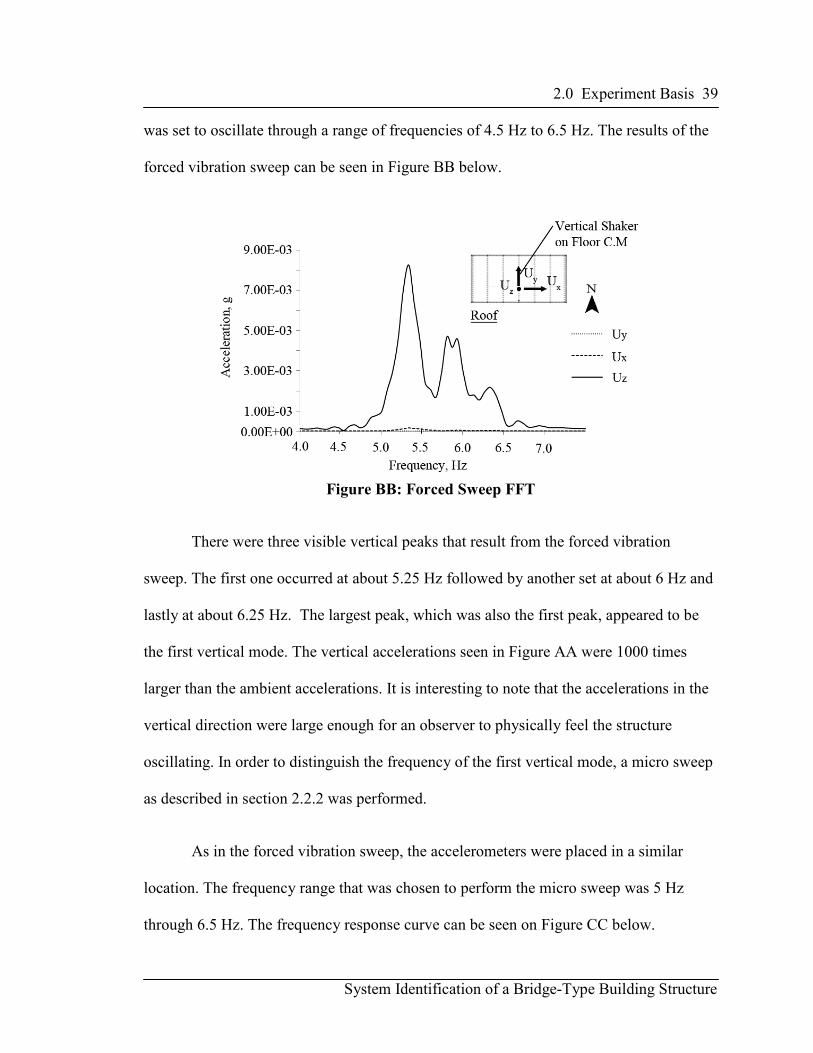
2.0 Experiment Basis 39
System Identification of a Bridge-Type Building Structure
was set to oscillate through a range of frequencies of 4.5 Hz to 6.5 Hz. The results of the
forced vibration sweep can be seen in Figure BB below.
Figure BB: Forced Sweep FFT
There were three visible vertical peaks that result from the forced vibration
sweep. The first one occurred at about 5.25 Hz followed by another set at about 6 Hz and
lastly at about 6.25 Hz. The largest peak, which was also the first peak, appeared to be
the first vertical mode. The vertical accelerations seen in Figure AA were 1000 times
larger than the ambient accelerations. It is interesting to note that the accelerations in the
vertical direction were large enough for an observer to physically feel the structure
oscillating. In order to distinguish the frequency of the first vertical mode, a micro sweep
as described in section 2.2.2 was performed.
As in the forced vibration sweep, the accelerometers were placed in a similar
location. The frequency range that was chosen to perform the micro sweep was 5 Hz
through 6.5 Hz. The frequency response curve can be seen on Figure CC below.

2.0 Experiment Basis 40
System Identification of a Bridge-Type Building Structure
Figure CC: Frequency Response Curve
The maximum acceleration at the roof occurred at a frequency of 5.33 Hz. The
response for this particular mode was sensitive to the change in frequency; therefore the
damping ratio for the first vertical mode was about 1.50%. The vertical shaker was placed
at the center of mass of the floor diaphragm and set up to continuously oscillate at the
natural frequency 5.33 Hz. Similar as in the translational modes, 70 locations were used
to record the N-S, E-W, and vertical accelerations throughout the structure’s floor and
roof diaphragms. Figure DD below illustrates an isometric view of the first vertical mode.

2.0 Experiment Basis 41
System Identification of a Bridge-Type Building Structure
Figure DD: First Experimental Vertical Mode Shape
Figure DD is an isometric view of the vertical accelerations in the first mode
shape. The primary motion of this mode was in the vertical direction, thus it was shown
as an isometric rather than in plan.
As expected, the first mode of vibration in the vertical direction was the floor and
roof diaphragm vibrating in phase with each other amid a deflected shape of a half sine
wave. A maximum steady state acceleration of 55 mg was experienced at the center of
mass of the roof diaphragm, 6,875 times larger than the ambient vertical accelerations.
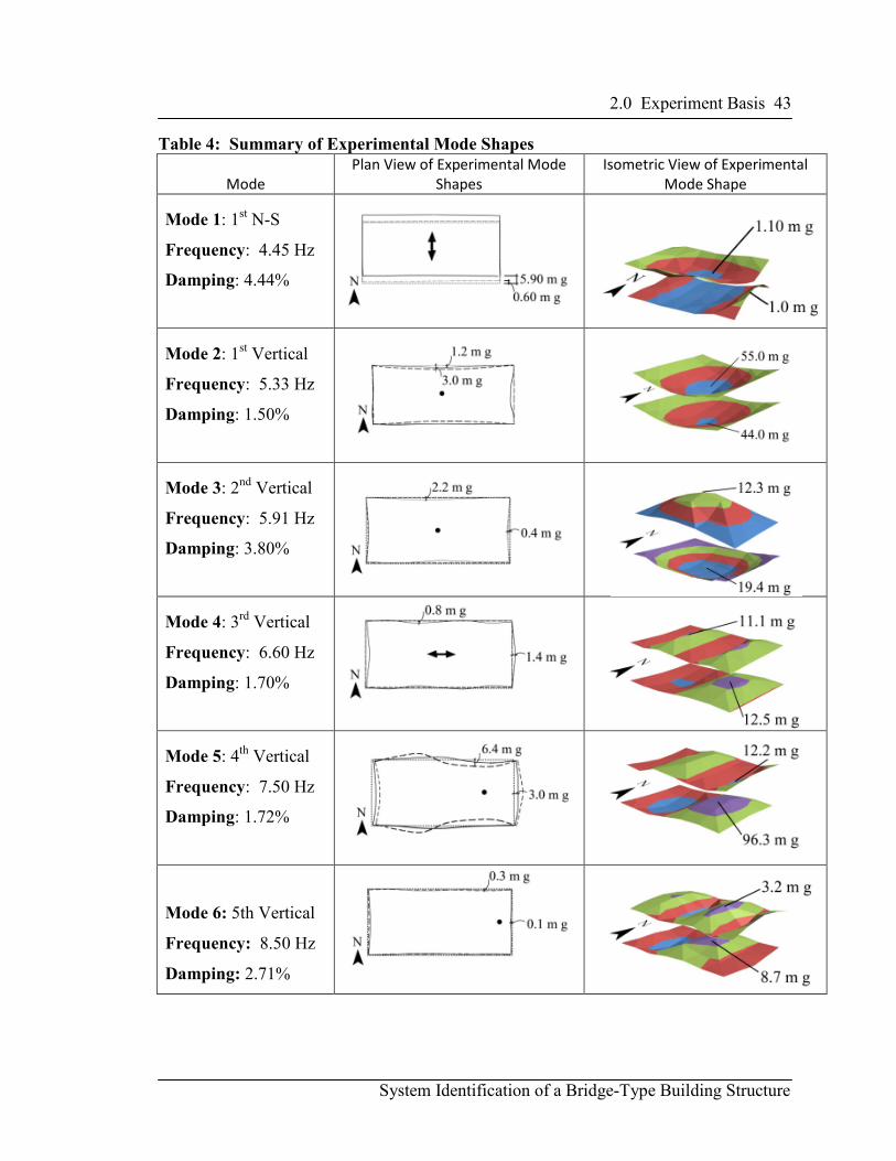
A total of 9 mode shapes were recorded. For simplicity, only the first two
translational and first vertical modes (denoted modes 1, 2 and 7 in Table 4 on page 43)
were explained in detail. Table 4 below is a summary of all 9 mode shapes. Please note
that all subsequent discussions will refer to the experimental mode shapes as apparent
mode shapes prior to performing the sweeping procedure. The sweeping procedure is a
purification process of the experimental apparent mode shapes. A further explanation can
be read in section 3.2 of this thesis.

2.0 Experiment Basis 42
System Identification of a Bridge-Type Building Structure
The first column on the left of Table 4 contains a brief description of the apparent
mode. The middle column is a plan view of the translational accelerations, and the far
right column is an isometric view of the vertical accelerations.
2.0 Experiment Basis 43
System Identification of a Bridge-Type Building Structure
Table 4: Summary of Experimental Mode Shapes
Mode
Plan View of Experimental Mode
Shapes
Isometric View of Experimental
Mode Shape
Mode 1: 1st N-S
Frequency: 4.45 Hz
Damping: 4.44%
Mode 2: 1st Vertical
Frequency: 5.33 Hz
Damping: 1.50%
Mode 3: 2nd
Vertical
Frequency: 5.91 Hz
Damping: 3.80%
Mode 4: 3rd
Vertical
Frequency: 6.60 Hz
Damping: 1.70%
Mode 5: 4th
Vertical
Frequency: 7.50 Hz
Damping: 1.72%
Mode 6: 5th Vertical
Frequency: 8.50 Hz
Damping: 2.71%

2.0 Experiment Basis 44
System Identification of a Bridge-Type Building Structure
Table 5 Continued: Summary of Experimental Mode Shapes
Mode 7: 1st E-W
Frequency: 9.10 Hz
Damping: 6.66%
Mode 8: 6th Vertical
Frequency: 9.50 Hz
Damping: 1.47%
Mode 9: Rotational
Frequency: 10.30 Hz
Damping: 4.00%
Apparent mode 3 was the second vertical mode at a frequency of 5.91 Hz. It was
similar to apparent mode 2 with the exception that the roof and floor diaphragms vibrated
out of phase. The damping ratio was 3.80%, 2.5 times more than apparent mode 2.
Damping can decrease the acceleration demands which as seen in apparent mode 3, the
maximum acceleration was about 2.25 times less than the maximum floor acceleration in
apparent mode 2. Coupling of apparent modes 2 and 3 occurred due to the fact that the
frequencies of the two apparent modes were less than 0.75 Hz apart and also due to the
fact that the two apparent modes were excited in the same location.
The natural frequency for apparent mode 4 was experimentally determined to be
at 6.60 Hz. Apparent mode 4 was unique in the sense that it was a vertical mode found by

2.0 Experiment Basis 45
System Identification of a Bridge-Type Building Structure
applying the horizontal shaker in the E-W direction. The shaker was mounted to the
underside of the middle wide-flange roof beam; because it was applied to the underside
of the beam, it initiated torsion into the beam, which caused out-of-plane deformation of
the roof diaphragm. It is interesting to note that although apparent mode 4 was excited
using the horizontal shaker, the vertical accelerations were almost 9 times more than the
translational accelerations. The apparent mode shape was defined by the out-of-plane
deformations of the roof and floor diaphragms. The roof created a deflected shape that
appeared as two sine waves, whereas the floor only deformed into one sine wave.
Apparent mode 5 was the 4th
vertical mode with a frequency of 7.50 Hz. It was
excited using the vertical shaker at the east quarter point of the floor diaphragm.
Although apparent mode 4 and 5 were similar, the differences were in the acceleration
demands on the floor diaphragm and the roof’s deflected shape. The largest acceleration
in apparent mode 5 was 96.3 m g, about 8 times more than the accelerations in apparent
mode 4. In general the roof diaphragm in apparent mode 5 experienced maximum
accelerations where they were essentially zero in apparent mode 4.
Apparent mode 6 was excited with the vertical shaker on the east end of the floor
where the natural frequency was determined to be 8.50 Hz. Apparent mode 6 was a
vertical mode where the roof diaphragm resembles that of apparent modes 5, 7 and 8. The
floor’s deflected shape appeared that of a 1 ¼ sine wave. The accelerations throughout
the building were considerably less than any other apparent vertical mode. The damping
ratio was calculated to be 2.71% and aside from apparent mode 3, the damping ratio was
larger than all other apparent vertical mode. The low accelerations in apparent mode 6
2.0 Experiment Basis 46
System Identification of a Bridge-Type Building Structure
could have resulted from the placement of the vertical shaker. The shaker was placed
approximately 4 ft from the east end support where the oscillating 30-lb force was
absorbed by the stiff support, ineffectively exciting the structure.
Apparent mode 8 was a third order vertical mode. Its response was also
dominated by the out-of-plane deformation in the diaphragms; however, the response was
not nearly as strong as the previously mentioned vertical modes. The damping ratio was
also relatively low at 1.47%. The out-of-plane deformation of the floor was defined by 1
½ sine waves, whereas the roof was defined by 2 sine waves.
Apparent mode 9 was a rotational mode that was excited by placing the shaker on
the roof at a 45 degree angle on the N-E end of the building. The damping ratio was
calculated to be 4.0%. Apparent mode 9, rotation about the vertical axis, experienced
considerable vertical accelerations on both the floor and roof diaphragms that seemed to
be similar to the vertical accelerations in apparent mode 8.
2.5 Modal Orthogonality of Experimental Mode Shapes
One of the fundamental principles in structural dynamics is the orthogonality of
the eigenvalue solutions (Chopra 2007). When ωj ≠ ωi
ij Mφφ = 0 Equation 20
Two modes with distinct frequencies are 90 degrees out of phase with each other
if the result of equation 20 is equal to zero. When ωj = ωi

2.0 Experiment Basis 47
System Identification of a Bridge-Type Building Structure
ij Mφφ = 1 Equation 21
Equation 21 is equal to 1 if the ith and jth modes are in phase with each other.
Both equation 20 and equation 21 are theoretical solutions when two modes are either out
of phase or in phase with each other, respectively. When conducting experimental FVT,
the results between two different modes will never yield a solution of 1.
Similar to equation 20 and equation 21, another frequently used correlation tool is
the modal assurance criterion (MAC). A MAC number is a statistical indicator used
(Allemang 2003) to define the consistency (degree of linearity) between two sets of mode
shapes. The MAC also takes on a value from zero to unity where zero represents
inconsistent correspondence and unity represents a consistent correspondence. The MAC
number can be calculated using equation 22:
( )( )( )j
T
ji
T
i
j
T
i
φφφφφφ
MM
MMAC
2
= Equation 22
Where iφ and jφ represent the two mode shapes being compared, and
M is the mass matrix of the structure.
Apparent modes acquired through FVT will always have some interaction with
other modes. The severity of interaction depends if the mode of interest is excited in an
ideal location. For example, placing the vertical shaker at a quarter point (a non-ideal
location for apparent modes 2 or 3) of the floor diaphragm will possibly excite apparent
modes 2, 3, 4, 5 and 6. Apparent modes 7, 8 and 9 will not be excited because apparent
mode 7 and 9 are considered non vertical modes and the quarter point in apparent mode 8

2.0 Experiment Basis 48
System Identification of a Bridge-Type Building Structure
occurs at a node of the deflected shape. The ideal location for shaker placement would be
where the peak response of the apparent mode occurs, see Table 4 on page 43. A further
explanation of ideal shaker locations will be given later in this section.
Applying equation 22 will yield a range of solutions of 0 < x < 1, where x is the
correlation between the ith and jth mode. Table 6 below is a matrix of MAC numbers
comparing experimental results.
Table 6: Mass Weighted Correlation Numbers Comparing Experimental Mode
Shapes
1 2 3 4 5 6 7 8 9
1 1.00 0.00 0.00 0.00 0.00 0.00 0.01 0.00 0.09
2 0.00 1.00 0.04 0.00 0.00 0.01 0.00 0.01 0.00
3 0.00 0.04 1.00 0.00 0.00 0.01 0.00 0.00 0.00
4 0.00 0.00 0.00 1.00 0.01 0.01 0.01 0.00 0.00
5 0.00 0.00 0.00 0.01 1.00 0.41 0.02 0.00 0.00
6 0.00 0.01 0.01 0.01 0.41 1.00 0.12 0.19 0.00
7 0.01 0.00 0.00 0.01 0.02 0.12 1.00 0.00 0.00
8 0.00 0.01 0.00 0.00 0.00 0.19 0.00 1.00 0.00
9 0.09 0.00 0.00 0.00 0.00 0.00 0.00 0.00 1.00
Note that the diagonal values in Table 6 correspond to the condition in Eq. 21,
thus the values are equal to 1.
Apparent modes 1 and 9 had a correlation of 0.09. Apparent mode 9 was the
apparent rotational mode, and apparent mode 1 was the N-S mode. Although both were
excited at two different shaker locations, the apparent rotational mode did not contain
some N-S translational motion. Thus apparent modes 1 and 9 yield a correlation of 0.09.

2.0 Experiment Basis 49
System Identification of a Bridge-Type Building Structure
Apparent mode 6 had correlations of 0.41, 0.12 and 0.19 with apparent modes 5, 7
and 8, respectively. Apparent modes 5, 6, and 8 were excited on the east end of the floor
using the vertical shaker and showed in similar out-of-plane motion of the roof
diaphragm. Apparent mode 7 was considered a translational mode but because the
relative stiffness of the lateral system to the diaphragm is substantially large, the roof
diaphragm underwent significant out-of-plane deformation.
The interaction of apparent mode 6 with apparent modes 5, 7, and 8 indicated that
there was a possibility that apparent mode 6 was not a real mode. Interaction of apparent
modes naturally occurs in forced vibration testing; however, the degree of interaction can
be minimized when the shaker is placed at the most optimal location. Apparent mode 6
was excited with the vertical shaker placed on the floor on the east end of the structure. If
apparent modes 5, 7, and 8 are examined in Table 4, one can conclude vertical
accelerations at the location where the vertical shaker was placed are in existence. Thus
what appeared to be apparent mode 6 was simply the response of the structure composed
of apparent modes 5, 7, and 8.
For future research, because the real mode 6 was not found, it is suggested that
the vertical shaker be placed in a location that will maximize the response of mode 6
while minimizing the response of all other modes. Figure EE shows elevation views of
apparent modes 2, 3, 4, 5, and 6 with a proposed location for placement of the vertical
shaker in an attempt to capture the real mode 6.

2.0 Experiment Basis 50
System Identification of a Bridge-Type Building Structure
Figure EE: Future Placement of Vertical Shaker to Optimize Apparent Mode 6
To capture the real mode 6, it is proposed to place the vertical shaker on the floor
12 ft from the south face at a frequency that shall be determined by the same procedures
explained earlier in sections 2.2 through 2.4. The proposed new location for the vertical
shaker would be within the vicinity of the maximum accelerations for apparent modes 2
and 3 occur, and although this location will minimize the response of apparent modes 4
and 5, some interaction between apparent mode 6 with apparent modes 2 and 3 may
occur. However there is a possibility that the frequencies between the apparent modes
may be distant enough that apparent modes 2 and 3 will not be excited.

2.0 Experiment Basis 51
System Identification of a Bridge-Type Building Structure
2.6 Experimental Findings
Interesting findings through FVT were diaphragm flexibility, frequency shift due to
temperature effects, a vertical anomaly on the floor diaphragm in the apparent N-S mode,
and foundation flexibility.
2.6.1 Roof Diaphragm Flexibility
As previously discussed in section 2.2, the roof diaphragm in the apparent N-S
mode behaved as a nearly rigid diaphragm. See Figure FF below.
Figure FF: N-S Experimental Mode Shape
In the apparent E-W mode, different responses among the roof beams become an
overall part of the apparent E-W mode. Thus, for clarification they were also included in
Figure FF. Figure GG below illustrates the flexibility in the roof diaphragm for the
apparent E-W mode.

2.0 Experiment Basis 52
System Identification of a Bridge-Type Building Structure
Figure GG: E-W Apparent Mode Shape
Research has been shown that for buildings with diagonal braces as the LFRS, the
in-plane flexibility of the floor and roof diaphragms may significantly influence the
dynamic behavior of building structures. Specifically for single story steel buildings, the
in-plane stiffness of the roof diaphragm are magnitudes smaller than the stiffness of the
LFRS (Trembley and Stiemer 1996).
Some major factors that contribute to the flexibility of the diaphragm are warping
of the panel, slip of the connections, and the geometry of the steel deck panel (Luttrell
1995). In addition to the diaphragm not being properly attached to the roof gravity
beams; on-site inspections lead to speculate that there was no interlocking connection
between the 2-ft wide steel deck panels. The roof diaphragm is composed of rigid
insulation topped with gravel that is supported by wide flange gravity beams at 8-ft on
center. To preserve the state of the Bridge House, a non-destructive analytical parametric
study was performed in an attempt to estimate the diaphragm stiffness.

2.0 Experiment Basis 53
System Identification of a Bridge-Type Building Structure
The side lap connection (connector slip parameter) between the panels can
significantly influence the diaphragm stiffness. Thus, three types of connections that were
investigated. See Figure HH below.
Figure HH: Steel Deck Panel Connections A) Seam Weld B) Button Punch C) Screw
The three different connections evaluated in this parametric study are used in
current practice, whereas only the seam weld and button punch was used at the time the
Bridge House was built. Equation 23 is provided by the Steel Deck Institute’s (SDI)
Diaphragm Design Manual to estimate the shear modulus of a steel deck diaphragm:
( ) CDd
sυ12
Et'G
n +++= Equation 23
Where G’ is the shear modulus defined by Eq.1,
E is the modulus of elasticity,
t is the base metal thickness,
nD is the warping constant,
C is the connector slip parameter,
s is the girth of corrugation per rib,
d is the corrugated pitch, and
ν is Poisson’s ratio, 0.3.

2.0 Experiment Basis 54
System Identification of a Bridge-Type Building Structure
Medhekar and Kennedy (1997) investigated the response of a low rise steel building
under seismic ground motion and adapted equation 24 to determine the natural period of
a low rise steel building.
gKK
WKK2πT
DB
DB += Equation 24
Where KD is the diaphragm stiffness defined by equation 25,
KB is the lateral stiffness of the vertical bracing,
W is the seismic weight,
g is gravity.
With,
bG'
L
EIπ
L
πK
2
3
2
D
+= Equation 25
Where L is the length of the diaphragm,
EI is bending stiffness of the diaphragm,
G’ is the shear modulus of the diaphragm defined by equation 23,
b is the width of the diaphragm.
Equation 24 accounts for all significant characteristics of low rise steel buildings
with flexible roof diaphragms and yields excellent results when compared to more
elaborate numerical methods.
Each 2-ft wide deck panel in the Bridge House are 24-ft long and are supported
by wide flange beams at 8 ft on center as seen in Figure II below.

2.0 Experiment Basis 55
System Identification of a Bridge-Type Building Structure
Figure II: Roof Steel Deck Panel Configuration
The shear stiffness of the diaphragm was calculated using equations provided by
the Steel Deck Institute (SDI) (Luttrell 1995). Table 7 below is a summary of results
using equation 23, 24, and 25 for the three different connection types. Where G’ is the
diaphragm shear modulus, KD is the diaphragm stiffness and f is the natural frequency
calculated by taking the inverse of equation 24.
Table 7: Diaphragm Stiffness and Natural Frequency of the Analytical E-W Mode
for Different Connections Types
Button
Punch Screws Welds
ns G' KD f G' KD f G' KD f
0 27.6 543.9 11.1 27.6 543.9 11.1 27.6 543.9 11.1
3 28.3 557.5 11.2 34.4 676.3 11.9 43.1 847.0 12.7
6 29.0 571.1 11.3 40.7 799.9 12.5 56.4 1105.7 13.6
9 29.7 584.6 11.3 46.6 915.5 13.0 67.8 1328.8 14.2
12 30.4 598.0 11.4 52.2 1023.8 13.4 77.8 1523.4 14.6
16 31.3 615.7 11.5 59.0 1158.0 13.8 89.4 1747.1 15.0
As previously stated, the steel deck sheets are 24 ft long and are supported by
gravity beams. The number of side lap connections for this parametric study is located in
the far left column of Table 6, denoted as ns. For example, when ns = 3, 3 evenly spaced

2.0 Experiment Basis 56
System Identification of a Bridge-Type Building Structure
connections per 24-ft panel are considered. In past and current practice it is common to
spot weld the steel deck to the steel beams, thus for calculation purposes, spot welds were
assumed to be used where the diaphragm was connected to the gravity beams.
As a baseline the experimental natural frequency of the apparent E-W mode was
used as reference. From examination of Table 7, as the density of all connections
increased, the diaphragm stiffness and the natural frequency of the analytical E-W mode
also increased. It was also observed that welded side lap connections provided the most
stiffness while button punch connections offered the least. Although all of the results
overestimated the experimental natural frequency (9.10 Hz), a 22% error arose as a result
of assuming there are no connections between the side laps. Note that the parametric
study did not account for the additional flexibility from the missing restraints between the
steel deck panels and their supporting beams. As previously explained, it was
experimentally determined that a portion of the gravity roof beams were fully attached to
the metal deck while some were partially attached. In general, test results lead to believe
that the steel deck was only welded at each ends of the 24-ft long sections. If the
calculations performed per SDI were to account for the current conditions, the stiffness of
the diaphragm would have decreased and would have yielded better analytical results.
Three steel deck interlocking connections were evaluated; each connection
generated different results for the analytical frequency of the E-W mode. In comparison
to the experimentally determined natural frequency of the apparent E-W mode, the
analytical results were best when it was assumed that no interlocking connection between
the steel deck panels existed. Thus the results of the parametric study lead to believe that

2.0 Experiment Basis 57
System Identification of a Bridge-Type Building Structure
there is no connection other than friction between the steel deck panels. As a result, the
diaphragm provides minimal bending resistance in the E-W direction, and thus behaved
flexibly in the apparent E-W mode.
2.6.2 Temperature Effects
It was determined through FVT that the Bridge House, a steel structure, is
sensitive to increasing surrounding temperatures. During hot weather it was believed that
some of the steel elements in the LFRS of the structure elongated and went into
compression as a result of deformation compatibility, decreasing the structure’s
geometric stiffness which in turn affected the dynamic response of the structure. The
thermal phenomenon was observed and investigated only in the apparent N-S mode as
seen in Figure JJ below.
Figure JJ: N-S Experimental Mode Shape
The thermal phenomenon was first observed when the steady state accelerations
from the FVT in the apparent N-S mode significantly varied throughout the day. At the
time of testing, the sun consistently shined on the S-W end of the structure where as the
north face was sheltered by a flock of trees. See Figure KK below.

2.0 Experiment Basis 58
System Identification of a Bridge-Type Building Structure
Figure KK: Isometric on Site View of the Bridge House
In the morning, the south face of the Bridge House experienced rapid increase in
temperature and as the day progressed, the west end heated up and the south face cooled
down. The change in temperature experienced in the west and south faces throughout the
day were recorded to be 65 °F. The north and east end of the building were not exposed
to the sun, thus the temperature of the steel elements on those faces did not significantly
vary. To see the magnitude of this phenomenon, the surface temperature of the structure’s
west end was monitored and a frequency response curves for two different surface
temperatures were created (see Figure LL below). Various steel elements were exposed
throughout the day, thus the increase in temperature throughout the Bridge House was
non uniform. However, for an explanation of this phenomenon, only the west end of the
structure was investigated.

2.0 Experiment Basis 59
System Identification of a Bridge-Type Building Structure
Figure LL: Frequency Response Shift Due to Thermal Phenomena
When the surface temperature of the west end was at about 55 °F the natural
frequency of the apparent N-S mode was at about 4.5 Hz and when the temperature
increased to a temperature of 120°F, the natural frequency dropped to about 4.2 Hz, a 7
% decrease.
Figure MM below contains a multitude of frequency response curves that were
created throughout the day, summarizing the results of the steel surface temperature vs.
the natural frequency of the apparent N-S mode.

2.0 Experiment Basis 60
System Identification of a Bridge-Type Building Structure
Figure MM: Surface Temperature vs. Natural Frequency
At a surface temperature of about 55°F, the natural frequency of the apparent N-S
mode was about 4.5 Hz and from there on, the frequency decreased as the surface
temperature increased. The frequency reached a minimum of 4.2 Hz when the surface
temperature reached a maximum of 120°F. After a peak temperature of 120°F, the natural
frequency began to gradually climb back up. Although Figure MM contains an 11-hour
range of data, the natural frequency did not return to 4.5 Hz. However, FTVs performed
the following morning confirmed that the frequency was back to 4.5 Hz.
To further investigate this phenomenon, an analytical model was created where a
similar temperature change as in Figure MM was applied to the west end of the structure.
The deflected shape of the structure as a result of the temperature loading along with the
temperature induced compression stresses was illustrated on Figure NN below.

2.0 Experiment Basis 61
System Identification of a Bridge-Type Building Structure
Figure NN: Compression Stresses Due to Thermal Expansion
To simulate the experimental results, a thermal load of a 65 °F temperature
change was applied to the columns and girders on the structures west end. As the
structure heats up, the steel elements in Figure NN want to naturally expand against the
structure and its supports, inducing compression stresses in the floor and roof beams up
to 20% of the yield stress. Similar to a P-delta effect, the flexural stiffness of the
members in Figure NN decreased, causing the natural frequency to also decrease. To
observe the participation of the thermally affected steel elements in the N-S mode, an
elevation view of the analytical N-S mode was provided in Figure OO below.
Figure OO: East Elevation of First N-S Analytical Mode Shape

2.0 Experiment Basis 62
System Identification of a Bridge-Type Building Structure
Since the mass of the structure was unchanged the stiffness of the structure must
have decreased. Globally, as the temperature increased, the steel in the Bridge House
wanted to naturally expand; however, boundary conditions restrained the elements from
expanding thus resulting in compression. In the case of the apparent N-S mode, the P-
delta effect caused the flexural stiffness in the N-S direction to decrease, thus also
decreasing the natural frequency. This phenomenon was determined to only affect the
frequency of the apparent N-S mode. However, in order to globally understand the
thermal phenomenon, other modes should be evaluated to determine if other modes are
more, equally, or less affected. To better understand why the natural frequency is
sensitive as the temperature of the structure increases and insensitive as the temperature
decreases, additional research is recommended.
2.6.3 Vertical Anomaly on the Floor Diaphragm in First N-S Mode
The building was excited in the N-S direction; however, a vertical anomaly on the
floor diaphragm was consistently detected in the apparent N-S mode. Although the
primary motion of the building was N-S, significant vertical accelerations were evident
on the east end of the floor diaphragm. An isometric view of the vertical mass normalized
floor accelerations can be seen in Figure PP below.

2.0 Experiment Basis 63
System Identification of a Bridge-Type Building Structure
Figure PP: Mass Normalized Vertical Floor Accelerations of the N-S Mode
One test utilized a 30-lb force whereas the second test used a 3-lb force. The 3-lb
force test was established to examine if the 3-lb force was small enough to effectively
excite the structure without overcoming friction of the possible detached floor. The
steady state accelerations of the 3-lb test were 90% smaller than the results of the 30-lb
test; however, the global results of both tests were similar due to mass normalization.
The flexibility of the east end of the floor experienced a mass normalized
acceleration of 9.1x10⁻⁴
g, 1.6 times more than the normalized translational accelerations
of the floor as seen in Figure QQ below.
Figure QQ: Mass Normalized Translational Floor Accelerations of the N-S Mode

2.0 Experiment Basis 64
System Identification of a Bridge-Type Building Structure
The vertical accelerations observed are clearly from the contribution of another
mode. It is unknown as to why such a large vertical response is generated from
excitement of the structure in the N-S direction; however, it is reasonable to conclude that
from the FVT results, there is a lack of connection between the floor diaphragm and the
girder on the east end, causing the floor girder to thrust the floor diaphragm upward.
2.6.4 Foundation Flexibility
Experimental results suggest that foundation flexibility was an important
component of most of the apparent mode shapes. The foundations are 18- in x 18-in
concrete piers bearing on 4.5-ft x 4.5-ft concrete pads. All four foundation piers are
different in length as seen in Figure RR on below.
Figure RR: Configuration of Concrete Foundation Piers

2.0 Experiment Basis 65
System Identification of a Bridge-Type Building Structure
The pier denoted as F1 in Figure RR is almost completely embedded in the soil,
whereas F4 is almost completely exposed. The concrete piers are believed to be similar to
a cantilever beam where the stiffness of a pier is a function of its length. As a result, the
different pier heights would generate different lateral stiffness. Typically torsion arises
when a variation of stiffness occurs; however, the FVT results proved otherwise. By
examining the apparent mode shapes, it was reasonable to conclude that the soil bearing
against and on the concrete piers was not sufficient to engage the piers in bending,
causing concrete piers to rock in the apparent N-S and E-W mode. To illustrate the
motion of the foundations in the apparent N-S mode, Figure SS below provides the mass
normalized floor accelerations.
Figure SS: Mass Normalized Translational Floor
Accelerations of the N-S Mode Shape
The Bridge House was experimentally determined to be pin connected to the
foundations. Thus, due to deformation compatibility, if the floor was moving, so were the
foundations. To illustrate the motion of the foundations in the apparent E-W mode,
Figure TT below provides the mass normalized floor accelerations.

2.0 Experiment Basis 66
System Identification of a Bridge-Type Building Structure
Figure TT: Mass Normalized Translational Floor
Accelerations of the E-W Mode Shape
The apparent E-W mode was composed of translational E-W motion in
combination with significant roof vertical accelerations. The lateral stiffness of the LFRS
in the N-S direction is considerably less than the lateral stiffness of the foundations/soil
whereas on the other hand, the LFRS in the E-W direction is considerably larger. Thus as
a result, the floor in the apparent E-W mode laterally accelerated about 4 times more than
in the apparent N-S mode. To complete the illustration of the motion of the foundations
in three orthogonal directions, Figure UU below exhibits the mass normalized
translational floor accelerations of the 1st apparent vertical mode.
Figure UU: Mass Normalized Translational Floor
Accelerations for the First Vertical Mode Shape

2.0 Experiment Basis 67
System Identification of a Bridge-Type Building Structure
The 1st apparent vertical mode was dominated by in-phase out-of-plane motion of the
floor and roof diaphragm. Although predominantly was a vertical mode, the piers slightly
experienced lateral accelerations; however, they were not as significant as in the apparent
E-W and N-S mode.
The three mode shapes in Figure SS, TT and UU were illustrated to highlight the
lateral response of the concrete piers in three orthogonal apparent mode shapes.
Foundation flexibility can be observed in all three figures, thus it is reasonable to
conclude that foundation flexibility played an important role in the dynamic behavior of
the Bridge House.

3.0 Analytical Basis 68
System Identification of a Bridge-Type Building Structure
3.0 ANALYTICAL BASIS
The second part of this project was to develop an analytical model that accurately
captured the dynamic behavior of the Bridge House utilizing a methodology known as
system identification. System identification is an effective tool used to develop analytical
models from experimental data. Test-validated analytical models can stimulate the
understanding of real dynamic behavior, thereby creating an improved understanding of
the assumptions used in the analysis and design of a structure.
The original construction documents were not readily available. However the
structure is in an exposed condition, thus most of the modeling decisions were based on
what was physically seen in the structure. An essential component in the development of
the computational model was estimating the mass of the structure. Not having a good
estimation of the mass can result in significant inaccuracy of the modal parameters in the
computational model.
The intention of the analytical modeling process is to begin with a simple hand
analysis and end with a complex computational model, focusing on the refinement of the
computational model based on comparisons with experimental results.
3.1 Progression of Analytical Modeling
Translational modes and vertical modes are two distinct dynamic responses, thus
the progression of the analytical modeling was divided into 2 sections. The first section
elaborated on the translational modes, while the 2nd
elaborated on the vertical modes.

3.0 Analytical Basis 69
System Identification of a Bridge-Type Building Structure
Note that for the computational model, the mass of the roof and floor was evenly
distributed throughout both diaphragms. However, the existing window assemblies create
concentrated line masses along the perimeter of the floor. As a result, the rotational
inertia of the floor was underestimated, resulting in a smaller natural frequency.
Capturing the rotational mode was far beyond simply being within the range of the
experimentally determined natural frequency; discrepancies in the mode shapes indicate
that the structure’s rotational stiffness is too low and that there are significant vertical
accelerations in the experimental results not being captured by the computational model.
Due to the limited scope of this thesis, the rotational mode was excluded from this
portion of the thesis. The rotational mode is considered relatively insignificant in
comparison to the rest of the modes; however, for completeness the results were still
reported.
3.1.1 Translational Modes
The first attempt in trying to analytically model the Bridge House was done by
performing a simple hand analysis assuming a rigid roof diaphragm with a fixed base as
seen in Figure VV below.
Figure VV: Lumped Mass Rigid Diaphragm Mode
(Rendon)

3.0 Analytical Basis 70
System Identification of a Bridge-Type Building Structure
The frequency results for the hand analysis assuming a rigid diaphragm were 4.97
Hz for the N-S mode and 18.09 Hz for the E-W mode. Comparison to the experimental
results, shows a percent error of 11.68% and 98.80%, respectively. Experimental results
in Table 4 on page 43 for the N-S and E-W apparent modes indicate that the roof
diaphragm behaves nearly rigid in the apparent N-S mode and flexible in the apparent E-
W mode. Thus, use of the rigid diaphragm assumption can lead to an overestimation of
the natural frequency. Because diaphragm flexibility in low rise steel structures can
significantly decrease the natural frequency of a structure, a flexible diaphragm was
incorporated into the following computational model shown in Figure WW below.
Figure WW: Flexible Roof Diaphragm
The intent of the flexible diaphragm was to replicate the experimental results in
the apparent E-W mode. A fine mesh of out-of-plane elements in combination with the
roof gravity beams was used to generate the roof diaphragm as seen in Figure WW. The
thickness of the out-of-plane elements were calibrated to match the calculated mid span
deflection of a simply supported corrugated steel deck. Table 8 below is a summary of
the analytical results for a computational model with a flexible diaphragm.

3.0 Analytical Basis 71
System Identification of a Bridge-Type Building Structure
Table 8: Flexible Roof Diaphragm vs. Experimental Results
N-S Mode E-W Mode Rotational Mode
Analytical Frequency 3.58 Hz 6.13 Hz 5.27 Hz
Experimental Frequency 4.45 Hz 9.10 Hz 10.70 Hz
Percent Difference -19.60 % -32.60% -50.75 %
As previously mentioned, the in-plane flexibility of a diaphragm can significantly
decrease the natural frequency of the structure. A simple change of the diaphragm from
rigid to flexible caused the frequency in the N-S direction to drop to 3.58 Hz and 6.13 Hz
in the E-W direction, a 28% and 66% decrease from the previous model, respectively.
The analytical and experimental mode shape can be seen in Figure XX below.
Figure XX: Experimental vs. Analytical N-S Roof Mode Shape
Experimental results illustrated that the roof diaphragm was nearly rigid in the
apparent N-S mode. However, the analytical model resulted in an overly flexible
diaphragm. To increase the N-S in-plane stiffness, in-plane stiffness elements were
integrated to create a hybrid diaphragm as seen Figure YY below.
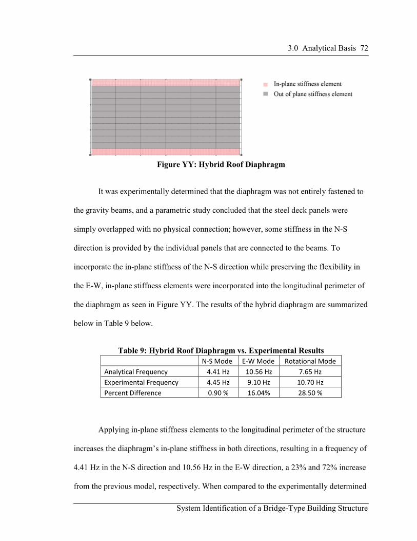
3.0 Analytical Basis 72
System Identification of a Bridge-Type Building Structure
Figure YY: Hybrid Roof Diaphragm
It was experimentally determined that the diaphragm was not entirely fastened to
the gravity beams, and a parametric study concluded that the steel deck panels were
simply overlapped with no physical connection; however, some stiffness in the N-S
direction is provided by the individual panels that are connected to the beams. To
incorporate the in-plane stiffness of the N-S direction while preserving the flexibility in
the E-W, in-plane stiffness elements were incorporated into the longitudinal perimeter of
the diaphragm as seen in Figure YY. The results of the hybrid diaphragm are summarized
below in Table 9 below.
Table 9: Hybrid Roof Diaphragm vs. Experimental Results
N-S Mode E-W Mode Rotational Mode
Analytical Frequency 4.41 Hz 10.56 Hz 7.65 Hz
Experimental Frequency 4.45 Hz 9.10 Hz 10.70 Hz
Percent Difference 0.90 % 16.04% 28.50 %
Applying in-plane stiffness elements to the longitudinal perimeter of the structure
increases the diaphragm’s in-plane stiffness in both directions, resulting in a frequency of
4.41 Hz in the N-S direction and 10.56 Hz in the E-W direction, a 23% and 72% increase
from the previous model, respectively. When compared to the experimentally determined

3.0 Analytical Basis 73
System Identification of a Bridge-Type Building Structure
frequencies, the analytical model yields a percent error of 0.90% for the N-S mode and
16.04% for the E-W mode. The analytical and experimental N-S mode shape can be seen
in Figure ZZ below.
Figure ZZ: Experimental vs. Analytical N-S Roof Mode Shape
The increase of the diaphragm’s in-plane stiffness is evident in Figure ZZ
resulting in a much improved correlation between the analytical and experimental results.
Creating a hybrid diaphragm allows for flexibility in the E-W direction while maintaining
the in-plane stiffness in the N-S direction. The analytical and experimental E-W mode
shape can be seen in Figure AAA below.
Figure AAA: Experimental vs. Analytical E-W Roof Mode Shape
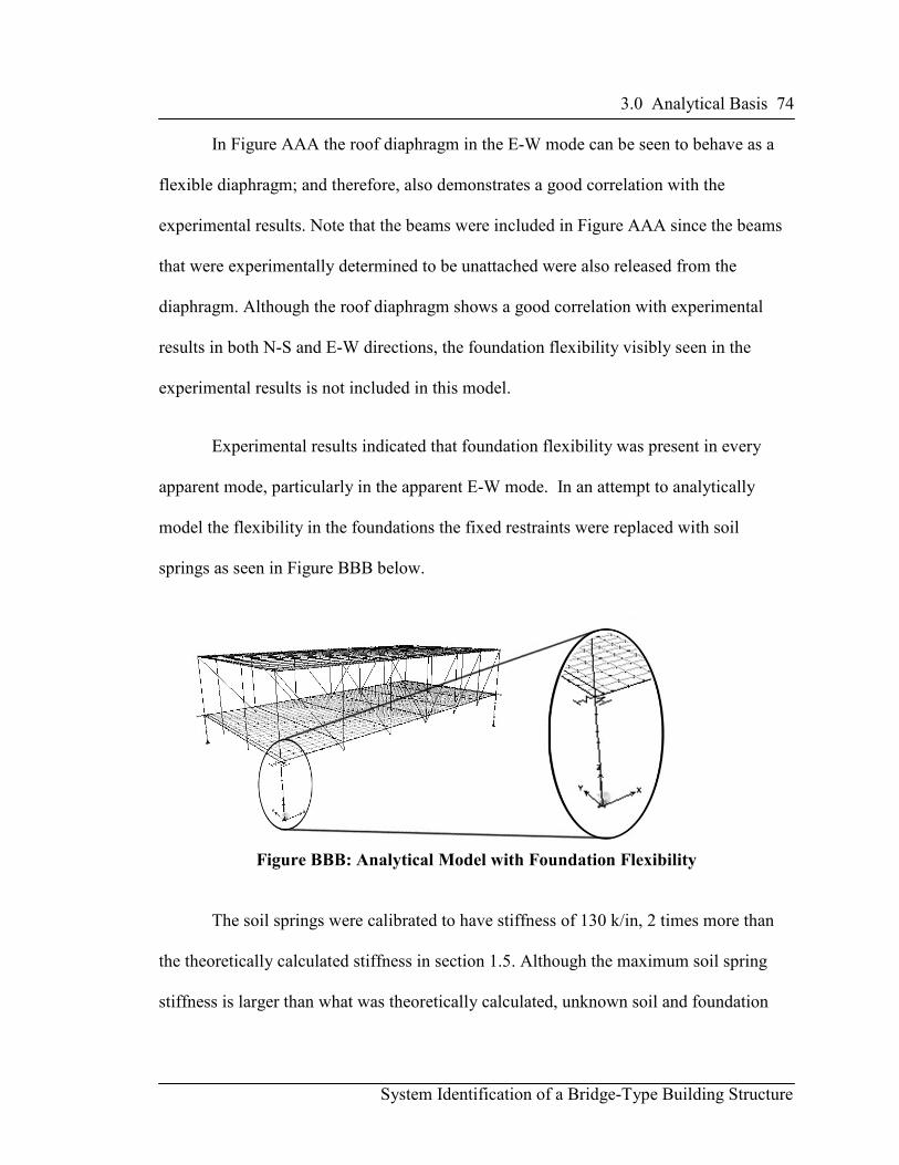
3.0 Analytical Basis 74
System Identification of a Bridge-Type Building Structure
In Figure AAA the roof diaphragm in the E-W mode can be seen to behave as a
flexible diaphragm; and therefore, also demonstrates a good correlation with the
experimental results. Note that the beams were included in Figure AAA since the beams
that were experimentally determined to be unattached were also released from the
diaphragm. Although the roof diaphragm shows a good correlation with experimental
results in both N-S and E-W directions, the foundation flexibility visibly seen in the
experimental results is not included in this model.
Experimental results indicated that foundation flexibility was present in every
apparent mode, particularly in the apparent E-W mode. In an attempt to analytically
model the flexibility in the foundations the fixed restraints were replaced with soil
springs as seen in Figure BBB below.
Figure BBB: Analytical Model with Foundation Flexibility
The soil springs were calibrated to have stiffness of 130 k/in, 2 times more than
the theoretically calculated stiffness in section 1.5. Although the maximum soil spring
stiffness is larger than what was theoretically calculated, unknown soil and foundation

3.0 Analytical Basis 75
System Identification of a Bridge-Type Building Structure
conditions can significantly alter the soil spring stiffness defined in equation 5 on page
19.
The average height of the piers was referenced from the original construction
drawings that were created in the early 1960’s. In 2011, the Bridge House senior project
team (Rehabilitation 2011) confirmed that portions of the structure were not constructed
in accordance with the original construction drawings. For example, braces on the short
ends of the building were shown in the plan but were never installed. Thus it is possible
that there is discrepancy between the foundation piers shown in the drawings and the on-
site conditions.
Three variables that can alter the soil spring stiffness are the modulus of subgrade,
average pier height, and the width of the concrete pads that support the concrete piers. In
order to obtain an accurate value for the soil’s modulus of subgrade, an in depth soil
investigation would have to be performed. However, based on good computational
results, an analytical soil spring stiffness of 130 k/in is considered ideal. In order to
generate a stiffness of 130 k/in, the modulus of subgrade reaction would have to be two
times more than the maximum textbook value of 65 k/ft3
(see section 1.5) , a scenario that
is quite unlikely. Another unknown variable that can alter the soil spring stiffness is the
average pier heights. While preserving a modulus of subgrade reaction of 65 k/ft3, the
average pier height would have to decrease from 5-ft-9-in to about 4-ft-0-in to obtain the
ideal soil spring stiffness, a scenario that is more likely. Lastly, dimensions of the
existing concrete pads also have an effect on the soil spring stiffness. The original
construction plans specify that the concrete pads are 4-ft-6-in wide; however, while also
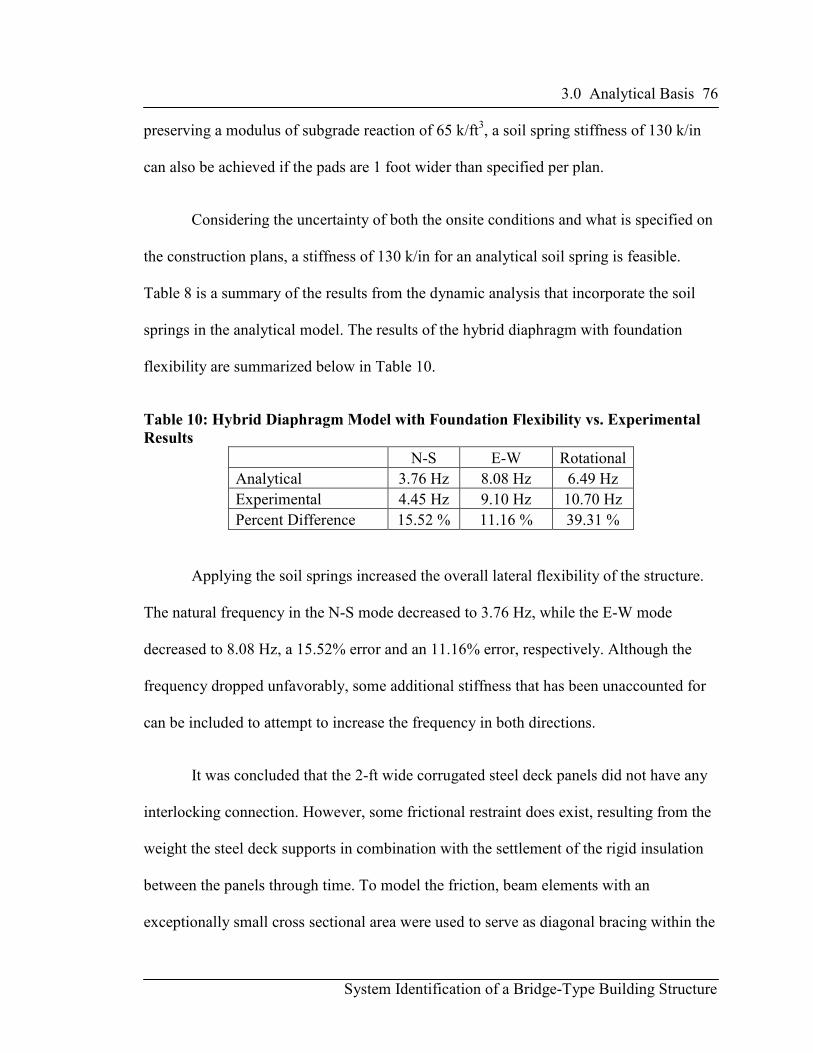
3.0 Analytical Basis 76
System Identification of a Bridge-Type Building Structure
preserving a modulus of subgrade reaction of 65 k/ft3, a soil spring stiffness of 130 k/in
can also be achieved if the pads are 1 foot wider than specified per plan.
Considering the uncertainty of both the onsite conditions and what is specified on
the construction plans, a stiffness of 130 k/in for an analytical soil spring is feasible.
Table 8 is a summary of the results from the dynamic analysis that incorporate the soil
springs in the analytical model. The results of the hybrid diaphragm with foundation
flexibility are summarized below in Table 10.
Table 10: Hybrid Diaphragm Model with Foundation Flexibility vs. Experimental
Results
N-S E-W Rotational
Analytical 3.76 Hz 8.08 Hz 6.49 Hz
Experimental 4.45 Hz 9.10 Hz 10.70 Hz
Percent Difference 15.52 % 11.16 % 39.31 %
Applying the soil springs increased the overall lateral flexibility of the structure.
The natural frequency in the N-S mode decreased to 3.76 Hz, while the E-W mode
decreased to 8.08 Hz, a 15.52% error and an 11.16% error, respectively. Although the
frequency dropped unfavorably, some additional stiffness that has been unaccounted for
can be included to attempt to increase the frequency in both directions.
It was concluded that the 2-ft wide corrugated steel deck panels did not have any
interlocking connection. However, some frictional restraint does exist, resulting from the
weight the steel deck supports in combination with the settlement of the rigid insulation
between the panels through time. To model the friction, beam elements with an
exceptionally small cross sectional area were used to serve as diagonal bracing within the

3.0 Analytical Basis 77
System Identification of a Bridge-Type Building Structure
diaphragm. The intention of the diagonal bracing was to slightly increase the in-plane
stiffness of the diaphragm and improve the correlation between the analytical and
experimental results. Figure CCC below is a plan view of the analytical model that
incorporates diagonal bracing in the roof diaphragm.
Figure CCC: Flexible Roof Diaphragm Model with Diagonal Bracing
The cross bracing spanned through the beams that were experimentally
determined to be un-attached to the steel deck. For example, beams 5 and 6 numbered
from left to right in Figure AAA on page 73 were experimentally determined to be free of
any connection to the diaphragm. Thus, just like the steel deck, the diagonal bracing also
spanned over beams 5 and 6. Table 11 below summarizes the results of the hybrid
diaphragm model with diagonal braces and foundation flexibility.
Table 11: Flexible Roof Diaphragm Model with Diagonal Bracing vs. Experimental
Results
N-S E-W Rotational
Analytical 4.10 Hz 8.20 Hz 7.38 Hz
Experimental 4.45 Hz 9.10 Hz 10.70 Hz
Percent Difference 7.86 % 9.89 % 31.02 %

3.0 Analytical Basis 78
System Identification of a Bridge-Type Building Structure
Applying the diagonal bracing in the roof diaphragm enhanced the overall lateral
in-plane stiffness of the diaphragm. The results can be seen in Table 11 above. Both the
natural frequencies of the N-S and E-W mode increased, resulting in an improved
correlation between the experimental and analytical results. The natural frequency of the
analytical N-S mode was 7.86% different, while the E-W mode was 9.89% different.
Figure DDD: Experimental vs. Analytical Flexible Roof Diaphragm Model with
Diagonal Bracing
Although the discrepancies are quite obvious in Figure DDD, the correlation
between the experimental and analytical results has improved. When compared to the
previous analytical model, the flexibility on the east end of the building has been reduced.
Stiffening the diaphragm also improved natural frequency for both the N-S and E-W
mode shapes.
Although the rotational mode was not discussed in detail in this thesis, Figure
EEE below illustrates the analytical and experimental mode shapes.

3.0 Analytical Basis 79
System Identification of a Bridge-Type Building Structure
Figure EEE: Analytical vs. Experimental Rotational Mode
As previously mentioned, capturing the rotational mode was far beyond simply
being within the range of the experimentally determined natural frequency; discrepancies
in the mode shapes indicate that the structure’s rotational stiffness is too low and that
there are significant vertical accelerations in the experimental results not being captured
by the computational model. As a result the correlation between the analytical and
experimental results is approximately zero.
There are many abnormalities in this structure. However, when compared to the
experimental results, the analytical model that incorporated the diagonal braces in the
roof diaphragm yielded the best results.
3.1.2 Vertical Modes
The Bridge House is a bridge structure, thus there were vertical modes that were
experimentally captured. As previously mentioned, there were a total of 6 vertical modes.
Utilizing the same analytical model that included the diagonal braces, a summary of
analytical results are compared to the experimental results in Table 12 below.

3.0 Analytical Basis 80
System Identification of a Bridge-Type Building Structure
Table 12: Analytical Vertical Modes vs. Experimental Vertical Modes
1st
Vertical
2nd
Vertical
3rd
Vertical
4th
Vertical
5th
Vertical
6th
Vertical
Model
Frequency 5.09 Hz 5.50 Hz N/A 6.74 Hz N/A 9.30 Hz
Experimental
Frequency 5.33 Hz 5.91 Hz 6.60 Hz 7.50 Hz 8.50 Hz 9.50 Hz
Percent
Difference 4.5 % 6.9 % N/A 10.1 % N/A 2.1 %
As shown in Table 12, the largest percent error calculated was 10.1% while the
lowest was 2.1%. The apparent 3rd
and 5th
experimental modes were not identifiable
through visual observation of the analytical deflected shapes; therefore, the percent errors
were not calculated for those two particular modes. It is a possibility that those two
particular modes were not captured in the computational model; however, that conclusion
cannot be drawn until a sweeping procedure is performed and correlation values between
the computational mode shapes and experimental modes are computed. A further
explanation on the sweeping procedure and correlation values also known as modal
assurance criterion (MAC) numbers will be in the subsequent section.
3.2 Comparison of Analytical to Experimental Mode Shapes
When a structure is excited by means of forced vibration at a natural frequency, the
mode of interest does not respond solely; the response of the structure naturally includes
the participation of other modes as well. Thus, every apparent mode captured is
considered to be diluted by other dynamic modes. The degree of dilution depends on the
placement of the shaker as previously discussed in section 2.5. In order to optimize the

3.0 Analytical Basis 81
System Identification of a Bridge-Type Building Structure
response of the structure, the shaker should be placed in a location where the response of
the mode of interest is most dominant.
To directly compare “pure” apparent mode shapes to analytical mode shapes, the
apparent mode shapes have to be purified as suggested by Gram-Schmidt (Golub 1989).
The purpose of purifying each apparent mode is to eliminate the participation of other
dynamic modes; however, in order to effectively purify each apparent mode, every
dynamic mode needs to be captured.
There were a total of 9 apparent modes that were experimentally captured in this
thesis. As indicated by Gram-Schmidt, the apparent modes should be organized from the
purest to the most diluted. Considering a mode “pure” assumes that the mode does not
contain any participation of other dynamic modes. Thus a judgment has to be made as to
which apparent mode is rationally considered most “pure”. In a conventional building
the most common dynamic modes in an “ultra low” force vibration test are the first two
translational and the rotational mode. With only three modes to choose from, the
sweeping procedure is clear-cut. However, having two translational, five vertical, and one
rotational mode to rearrange makes the procedure much more complex. Any change in
the arrangement of the modes will cause a significant change in the results, thus it is
important to organize the modes in a precise order.
In the first attempt to organize the apparent modes from purest to most diluted, it
was assumed that mode 1 was the “purest” followed by modes 5, 2, 3, 8, 6, 4, 9 and 7.
Mode 1 was chosen as the “purest” as its response was primarily translational motion in

3.0 Analytical Basis 82
System Identification of a Bridge-Type Building Structure
the N-S direction with very minimal out-of-plane motion in the roof and floor
diaphragms. Mode 5, a second order vertical mode, was chosen as the second purest as its
response was the strongest out of all 9 modes. Its peak acceleration was an out-of-plane
acceleration of 0.1g at the floor.
Modes 2 and 3 are coupled first order vertical modes. In mode 2 the out-of-plane
motion of the roof and floor diaphragms are in-phase, while in mode 3 the roof and floor
diaphragms are out-of-phase. The peak response of mode 2 is greater than mode 3 but
almost 2.5 times less than mode 5. Apparent mode 8 is a third order vertical mode and its
response is also dominated by well defined roof and floor out-of-plane deformations;
however, the vertical accelerations in apparent mode 8 are about 4 times less than
apparent mode 2.
Apparent modes 6, 4, 9, and 7 are considered to be the most diluted. AVTs and
FVTs for apparent mode 6 indicated that the vertical shaker should placed at mid span 4-
ft from the east end of the floor. However, this peculiar location (close a stiff support)
produced a well defined vertical mode with out-of-plane deformations in the roof and
floor. Apparent mode 4 is unique in the sense that it is a vertical mode found by applying
the horizontal shaker in the E-W direction. The shaker was mounted to the underside of
the middle wide-flange roof beam; because it was applied to the underside of the beam, it
initiated torsion into the beam, which caused out-of-plane deformation of the roof
diaphragm. Considering that both modes 6 and 4 are vertical modes, mode 6 was chosen
in front of mode 4 because mode 6 was found by utilizing the vertical shaker. Modes 9
and 7 are rotational and translational modes, respectively. Mode 7 was chosen as the most

3.0 Analytical Basis 83
System Identification of a Bridge-Type Building Structure
diluted due to the significant out-of-plane accelerations in the roof diaphragm. As
previously mentioned, it was concluded that the steel deck panels were not interlocked
with one another, and not all beams were properly attached to the steel deck. As a result
of these abnormalities, the response of apparent mode 7 was significantly affected.
Apparent modes 6 and 4 have similar roof out-of-plane deformations. In theory, by
placing apparent modes 6 and 4 in front of apparent mode 7, the out-of-plane
deformations of the roof diaphragm in mode 7 should get “swept out” by apparent modes
6 and 4.
In order to demonstrate the effect of the sweeping procedure, Table 13 below was
created. Table 13 is a matrix of MAC numbers in which the columns represent the
analytical mode shapes and the rows represent the apparent mode shapes.
Table 13: MAC Numbers Comparing Un-Swept-Apparent Results to Analytical
Results
In Table 13, the MAC numbers for apparent modes 1, 2, 3, and 5 were all above
0.90, which represents an excellent correlation. With a MAC number of 0.84, the un-
3.0 Analytical Basis 84
System Identification of a Bridge-Type Building Structure
swept apparent mode 8 correlates well with analytical mode 10. The un-swept apparent
mode 4 has MAC numbers of 0.49 and 0.42 with analytical modes 6 and 8, respectively.
As observed in Table 4 on page 43 the out-of-plane deformations of the floor diaphragm
in the apparent mode 4 resembled analytical mode 6, while the out-of-plane deformation
of the roof diaphragm in apparent mode 4 resembled analytical mode 8.
Un-swept apparent mode 6 has a MAC number of 0.50 with analytical mode 6.
Apparent mode 6 shows similar out-of-plane deformations in the floor diaphragm to
apparent mode 4. Lastly, un-swept apparent mode 7 have similar out-of-plane
deformation in the roof as in analytical mode 8 and similar translational displacement as
in analytical mode 9, which generates MAC numbers of 0.40 and 0.24, respectively. To
summarize the effect of the sweeping procedure, Table 14 below contains the MAC
numbers comparing the swept experimental results to the analytical results.
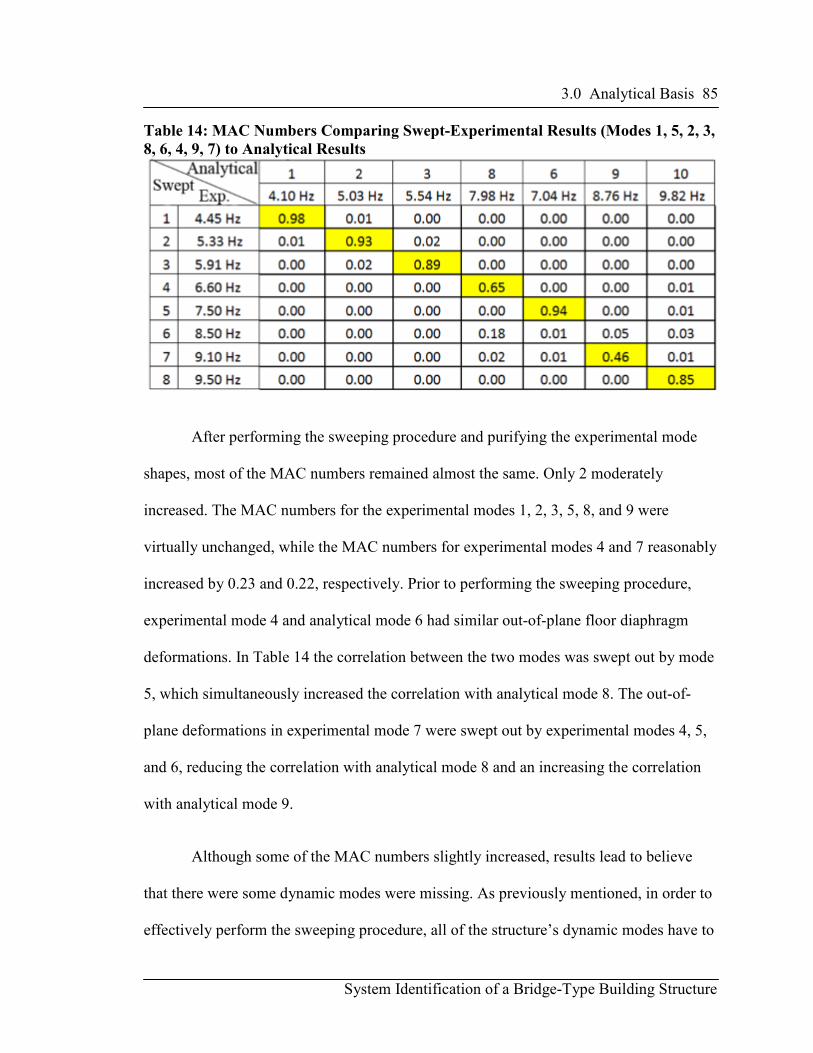
3.0 Analytical Basis 85
System Identification of a Bridge-Type Building Structure
Table 14: MAC Numbers Comparing Swept-Experimental Results (Modes 1, 5, 2, 3,
8, 6, 4, 9, 7) to Analytical Results
After performing the sweeping procedure and purifying the experimental mode
shapes, most of the MAC numbers remained almost the same. Only 2 moderately
increased. The MAC numbers for the experimental modes 1, 2, 3, 5, 8, and 9 were
virtually unchanged, while the MAC numbers for experimental modes 4 and 7 reasonably
increased by 0.23 and 0.22, respectively. Prior to performing the sweeping procedure,
experimental mode 4 and analytical mode 6 had similar out-of-plane floor diaphragm
deformations. In Table 14 the correlation between the two modes was swept out by mode
5, which simultaneously increased the correlation with analytical mode 8. The out-of-
plane deformations in experimental mode 7 were swept out by experimental modes 4, 5,
and 6, reducing the correlation with analytical mode 8 and an increasing the correlation
with analytical mode 9.
Although some of the MAC numbers slightly increased, results lead to believe
that there were some dynamic modes were missing. As previously mentioned, in order to
effectively perform the sweeping procedure, all of the structure’s dynamic modes have to

3.0 Analytical Basis 86
System Identification of a Bridge-Type Building Structure
be captured. Essentially, 9 modes may have not been enough. One of the essential modes
not recorded is a mode that is primarily composed of out-of-plane deformation of the roof
diaphragm. To effectively sweep out the out-of-plane deformations of the roof in
apparent mode 7, the missing mode needs to be captured. However, for computational
reasons, the apparent E-W mode was theoretically purified (artificially setting the vertical
roof accelerations in apparent mode 7 to zero) from the out-of-plane roof deformations
just as they would have been if the missing mode was recorded.
As a result of that assumption, the un-swept MAC number in Table 13 on page 83
for apparent mode 7 and analytical mode 9 significantly increased from 0.24 to 0.78. To
re-perform the sweeping procedure, the experimental modes were reorganized to reflect
the artificial purification of apparent mode 7. As previously explained, apparent modes 1,
5, 2, 3, and 8 are believed to be the “purest”, and thus were left in the same order. The
last four experimental modes were reorganized in the following order: 7, 4, 6, and 9.
Apparent mode 7 was moved to the front of the group as a result of its artificial
purification and aside from apparent mode 9, apparent mode 4 and 6 were extremely
diluted and are similar in shape. However, apparent mode 4 was chosen as more pure due
to a mass weighted correlation number of 0.41 (see Table 6 on page 48) between apparent
mode 6 and apparent mode 5. A value of 0.41 indicates a moderate correlation between
the two apparent modes and being that apparent mode 5 is considered the 2nd
most pure,
by default it is assumed that apparent mode 4 is as more pure between the two modes.
(see Table 4 on page 43). To summarize the effect of the second attempt at the sweeping

3.0 Analytical Basis 87
System Identification of a Bridge-Type Building Structure
procedure, Table 15 below contains the MAC numbers that compare the revised swept
experimental results to the analytical results.
Table 15: MAC Numbers Comparing Swept-Experimental Results (Modes 1, 5, 2, 3,
8, 7, 4, 6, 9) to Analytical Results
Overall the MAC numbers summarized in Table 15 are much improved over the
MAC numbers in Table 14. The MAC numbers for swept experimental modes 1, 2, 3, 5,
and 8 are unchanged and were previously discussed; therefore, this section will only
emphasize the MAC numbers for experimental modes 4, 6, 7, and 9.
As previously discussed, experimental mode 4 was found by exciting the structure
at the roof level in the E-W direction. Although it was primarily a vertical mode, some
translation deformation in the E-W direction can be seen as a result of the shaker
position. By virtue of the sweeping procedure, the translational deformations in
experimental mode 4 are swept out by experimental mode 7, resulting in a MAC number
of 0.76.

3.0 Analytical Basis 88
System Identification of a Bridge-Type Building Structure
Prior to performing the sweeping procedure, the out-of-plane deformations in the
roof diaphragm in experimental mode 7 were artificially swept out and resulted in a MAC
number of 0.78. After performing the sweeping procedure, the out-of-plane deformations
in the floor diaphragm were swept out by experimental mode 5, resulting in a much
improved MAC number of 0.86.
3.3 Analytical Model of Vertical Anomaly
An interesting anomaly that was found by virtue of forced vibration testing was a
vertical irregularity in the floor diaphragm in the N-S translational mode. As seen in
Table 4 on page 43, experimental mode 1 is dominated by the N-S translational motion of
the roof diaphragm; however, a vertical anomaly can be observed in the east end of the
floor and can also be seen in Figure FFF below.
Figure FFF: Experimental Vertical Floor Response of First N-S Mode
The vertical irregularity can be seen in Figure FFF on the east end of the floor
diaphragm. The vertical accelerations at this particular location were about 4 times
greater than the vertical accelerations at mid span. For clarification of the location of the
vertical anomaly, the floor plan of the Bridge House is shown in Figure GGG below.

3.0 Analytical Basis 89
System Identification of a Bridge-Type Building Structure
Figure GGG: Floor Plan
The vertical anomaly occurs at beam B7 as shown in Figure GGG. The assembly
of the floor diaphragm is composed of lightweight concrete over metal deck, which is
then supported by the wide flange beams as shown in Figure GGG. As previously stated,
the acceleration readings were taken from the top of the concrete slab, thus the vertical
anomaly results from the lack of connection between the metal deck and the wide flange
beam B7. In an attempt to capture similar behavior of the floor diaphragm, the analytical
model was modified so that the restraint between beam B7 and the floor diaphragm was
released. Figure HHH below is the analytical mode shape of the floor that best resembles
the vertical anomaly.
Figure HHH: Analytical of Model with Unconnected Beam (B7)

3.0 Analytical Basis 90
System Identification of a Bridge-Type Building Structure
The experimental and analytical results are not identical; however, there is a
resemblance between the two. The computed MAC number comparing both Figure FFF
and Figure HHH is 0.80. Although the results are promising, a more in-depth
investigation is needed to firmly conclude the as-built conditions of the Bridge House. It
should be noted that the modifications done to the analytical model, in order to capture
the dynamic mode seen in Figure HHH, were not included in the analytical model prior to
this section and were done only to confirm a possible explanation of the vertical anomaly.

4.0 Conclusions 91
System Identification of a Bridge-Type Building Structure
4.0 CONCLUSIONS
The Bridge House is a one story steel structure supported on 4 concrete piers that
spans 48 ft over a seasonal creek. The lateral force resisting system (LFRS) is composed
of ordinary moment frames in the N-S direction and braced frames in the E-W direction.
It is vertically supported by a pair of trusses.
An experimental investigation was performed by means of system identification
through ambient and forced vibration testing. Ambient vibration tests (AVT) were first
performed to determine the dominant response of the Bridge House in either the N-S, E-
W and vertical directions through a selected range of frequencies, an indication that a
possible mode was present. To better determine the natural frequency, AVT were
followed by forced vibration tests (FVT). FVT amplified the response of the structure
through the use of a linear mass shaker with an output force equivalent to 30 lbs.
An analytical model was developed to capture the dynamic behavior of the Bridge
House. The process of generating an accurate computational model required a series of
subsequent refined computational models based on comparisons with experimental
results.
4.1 AVT and FVT
Ambient Vibration Tests (AVT) was used to find the approximate range of all nine
natural frequencies. Forced Vibration Tests (FVT) was then performed to more
accurately determine the natural frequency of each mode. Once the natural frequency and
optimum shaker location was established, the shaker was positioned to continuously

4.0 Conclusions 92
System Identification of a Bridge-Type Building Structure
oscillate at each mode shape’s respective natural frequency. Mode shape mapping was
then used to determine the deformed shape of the structure at it respective resonant
frequency. Experimental mode shapes in this thesis are referred to as apparent mode
shapes prior to performing the sweeping procedure. To directly compare “pure”
experimental mode shapes to analytical mode shapes, the influence of other dynamic
modes on an apparent mode shape was minimized through the sweeping procedure.
The apparent N-S mode at 4.45 Hz was dominated by N-S translational motion.
The roof diaphragm behaved similar to that of a rigid diaphragm because the theoretical
N-S in plane stiffness of the diaphragm is 1.53 times greater than the lateral stiffness of
the moment frames. On the other hand, the apparent E-W mode was dominated by a
combination of translational and vertical accelerations where the diaphragm
demonstrated flexible behavior resulting from the theoretical E-W in plane diaphragm
stiffness being 2 times less than the lateral stiffness of the braced frames. The apparent E-
W mode also highlights that some roof beams were experimentally determined to be fully
attached, some partially attached and some not attached at all. The Bridge House spans
48 ft, thus vertical modes were also present in addition to the translational modes. A total
of 5 vertical modes were captured and vertical accelerations were recorded up to 0.1g.
During the experimental investigation interesting findings such as diaphragm
flexibility, foundation flexibility and frequency shifts due to thermal effects were found
throughout the mode shape mapping process.

4.0 Conclusions 93
System Identification of a Bridge-Type Building Structure
4.1.1 Diaphragms
The roof diaphragm is made up of rigid insulation topped with gravel supported by
2-ft x 24-ft metal deck. In the dynamic response of the structure, the roof diaphragm
behaved as flexible in the E-W direction whereas the same diaphragm behaved rigid in
the N-S direction. The E-W direction has an approximate stiffness of 1149 k/in, about 13
times stiffer than the N-S direction. The in-plane stiffness of the diaphragm in the E-W
direction is approximately 544 k/in. The diaphragm behaved differently in each direction
because the N-S direction is 53% less stiff than the N-S in-plane stiffness of the
diaphragm while the E-W direction provides 211% more stiffness than the E-W in-plane
stiffness of the diaphragm. As a result of the stiff lateral system, the diaphragm was
engaged in the apparent E-W mode and thus behaved flexibly. The in-plane stiffness of
the roof diaphragm was estimated by conducting a parametric study in accordance with
the Steel Deck Institute (SDI) where the experimentally determined E-W frequency was
used as a basis for comparison to the hand calculated results.
The type of side lap connections between the roof steel deck panels have a
significant effect on the in-plane stiffness which then effects the natural period of the
translational modes. During an on-site inspection there were no visual or physical
evidence of the type of connection between the steel deck panels. The roof diaphragm
connections that were considered in the parametric study were button punch, seam welds,
and screwed connections. It was analytically determined that a welded side lap
connection resulted in an E-W natural frequency of 15 Hz (a 65% error), whereas the
button punch connections resulted in a frequency of 11.5 Hz (a 26% error). The

4.0 Conclusions 94
System Identification of a Bridge-Type Building Structure
parametric study concluded that the steel deck panels were inter-linked with no physical
connection other than friction, producing a 22% percent difference from the
experimentally determined natural frequency. Note that the parametric study did not
account for the additional flexibility from the missing restraints between the steel deck
panels and their supporting beams. It was experimentally determined that a portion of the
gravity roof beams were fully attached to the metal deck while some were partially
attached. The lack of interlocking mechanism between the steel deck panels in
combination with the lack of restraints of the steel deck to the gravity beams produced a
highly flexible diaphragm. As a result, the ratio of the lateral stiffness to the diaphragm
in-plane stiffness is approximately 2 in the E-W direction versus 0.65 in the N-W
direction.
A vertical anomaly on the floor diaphragm was consistently detected in the apparent
N-S mode. The structure was excited in the N-S direction where its primary motion was
N-S; however, vertical accelerations up to 2 times greater than the lateral floor
accelerations were experienced on the east end of the floor diaphragm. The vertical
flexibility of the floor arose from the influence of a vertical mode resulting from the lack
of connection between the floor diaphragm and the floor beam at the east end of the
building.
4.1.2 Foundation Flexibility
The soil and the concrete foundation piers significantly contributed to the
translational response in the E-W direction; however, the contribution was negligible in
the N-S direction. Furthermore, the peak lateral roof to floor acceleration ratio was about

4.0 Conclusions 95
System Identification of a Bridge-Type Building Structure
2.7 in the E-W mode and about 9.8 in the N-S direction (4 times more in N-S than in the
E-W direction).
The concrete piers are no different than a cantilevered beam and the stiffness is a
function of its length, thus the different pier heights would typically result in different
lateral stiffness. Torsion arises when a variation of lateral stiffness occurs; however, the
results of the apparent E-W mode shape proved otherwise. The concrete piers have about
10% more lateral stiffness (based on ideal soil spring stiffness of 130 k/in) than the
surrounding soil. The ratio of lateral frame stiffness to soil spring stiffness is about 2.2 in
the E-W direction and about 0.15 in the N-S direction; thus, the soil bearing against and
on the concrete piers is not sufficient to engage the piers in bending, causing concrete
piers to rock, more so in the apparent E-W mode.
4.1.3 Frequency Shift Due to Thermal Effects
The Bridge House was experimentally determined to be sensitive to the measured
temperature range of 55 °F to 120 °F. Throughout the day as ambient temperature
progressively increased, the natural frequency of the N-S translational mode decreased
from 4.5Hz to 4.2Hz, a 7% decrease.
To computationally model this thermal phenomenon, an analytical model of the
Bridge House was created where a 65°F temperature change was applied to the steel
columns and girders of the LFRS on the west face of the structure (the side most
susceptible to sun exposure in the experimental N-S mode). As The Bridge House heats
up the steel expands against the structure and its supports, causing elements in the LFRS
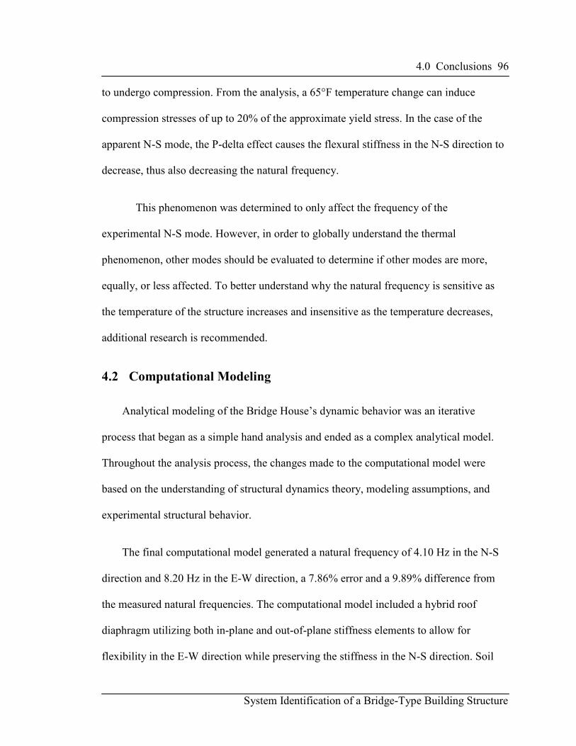
4.0 Conclusions 96
System Identification of a Bridge-Type Building Structure
to undergo compression. From the analysis, a 65°F temperature change can induce
compression stresses of up to 20% of the approximate yield stress. In the case of the
apparent N-S mode, the P-delta effect causes the flexural stiffness in the N-S direction to
decrease, thus also decreasing the natural frequency.
This phenomenon was determined to only affect the frequency of the
experimental N-S mode. However, in order to globally understand the thermal
phenomenon, other modes should be evaluated to determine if other modes are more,
equally, or less affected. To better understand why the natural frequency is sensitive as
the temperature of the structure increases and insensitive as the temperature decreases,
additional research is recommended.
4.2 Computational Modeling
Analytical modeling of the Bridge House’s dynamic behavior was an iterative
process that began as a simple hand analysis and ended as a complex analytical model.
Throughout the analysis process, the changes made to the computational model were
based on the understanding of structural dynamics theory, modeling assumptions, and
experimental structural behavior.
The final computational model generated a natural frequency of 4.10 Hz in the N-S
direction and 8.20 Hz in the E-W direction, a 7.86% error and a 9.89% difference from
the measured natural frequencies. The computational model included a hybrid roof
diaphragm utilizing both in-plane and out-of-plane stiffness elements to allow for
flexibility in the E-W direction while preserving the stiffness in the N-S direction. Soil
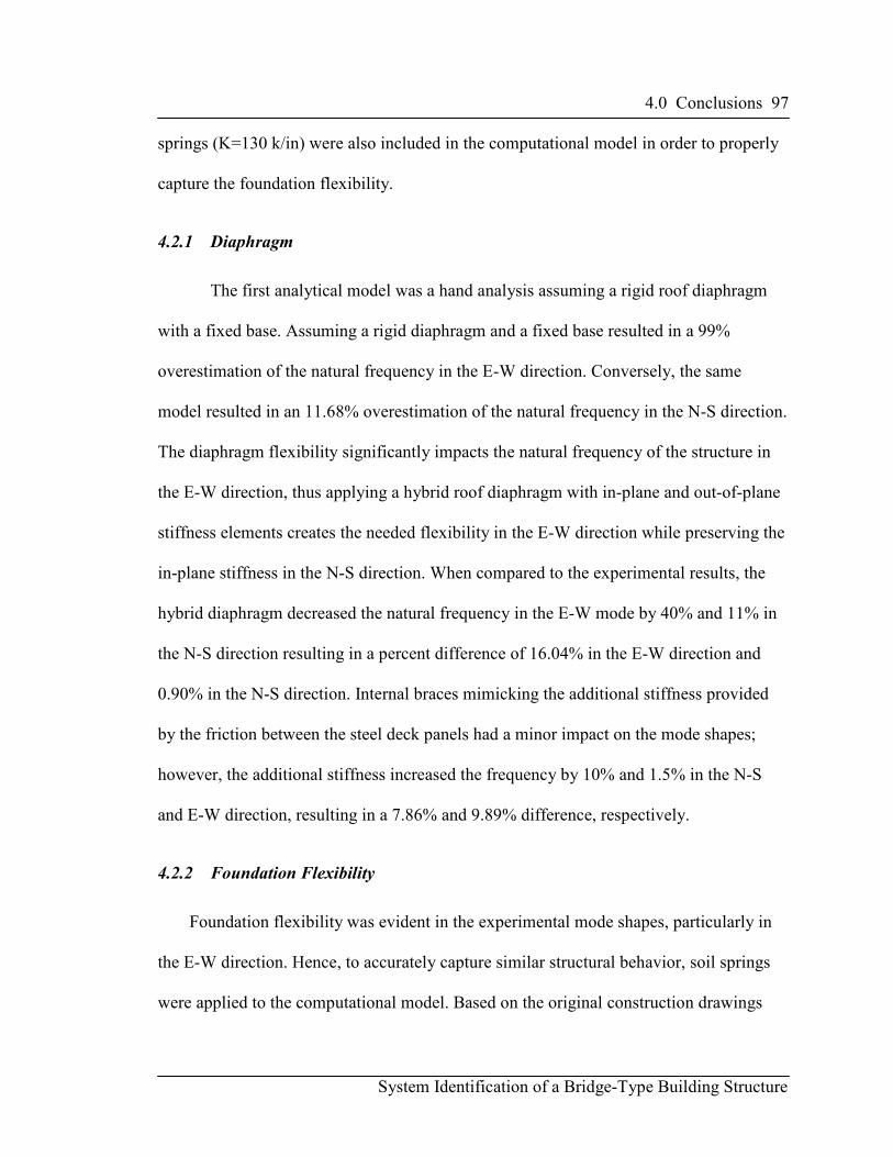
4.0 Conclusions 97
System Identification of a Bridge-Type Building Structure
springs (K=130 k/in) were also included in the computational model in order to properly
capture the foundation flexibility.
4.2.1 Diaphragm
The first analytical model was a hand analysis assuming a rigid roof diaphragm
with a fixed base. Assuming a rigid diaphragm and a fixed base resulted in a 99%
overestimation of the natural frequency in the E-W direction. Conversely, the same
model resulted in an 11.68% overestimation of the natural frequency in the N-S direction.
The diaphragm flexibility significantly impacts the natural frequency of the structure in
the E-W direction, thus applying a hybrid roof diaphragm with in-plane and out-of-plane
stiffness elements creates the needed flexibility in the E-W direction while preserving the
in-plane stiffness in the N-S direction. When compared to the experimental results, the
hybrid diaphragm decreased the natural frequency in the E-W mode by 40% and 11% in
the N-S direction resulting in a percent difference of 16.04% in the E-W direction and
0.90% in the N-S direction. Internal braces mimicking the additional stiffness provided
by the friction between the steel deck panels had a minor impact on the mode shapes;
however, the additional stiffness increased the frequency by 10% and 1.5% in the N-S
and E-W direction, resulting in a 7.86% and 9.89% difference, respectively.
4.2.2 Foundation Flexibility
Foundation flexibility was evident in the experimental mode shapes, particularly in
the E-W direction. Hence, to accurately capture similar structural behavior, soil springs
were applied to the computational model. Based on the original construction drawings
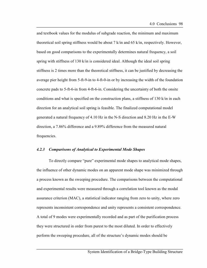
4.0 Conclusions 98
System Identification of a Bridge-Type Building Structure
and textbook values for the modulus of subgrade reaction, the minimum and maximum
theoretical soil spring stiffness would be about 7 k/in and 65 k/in, respectively. However,
based on good comparisons to the experimentally determines natural frequency, a soil
spring with stiffness of 130 k/in is considered ideal. Although the ideal soil spring
stiffness is 2 times more than the theoretical stiffness, it can be justified by decreasing the
average pier height from 5-ft-9-in to 4-ft-0-in or by increasing the width of the foundation
concrete pads to 5-ft-6-in from 4-ft-6-in. Considering the uncertainty of both the onsite
conditions and what is specified on the construction plans, a stiffness of 130 k/in in each
direction for an analytical soil spring is feasible. The finalized computational model
generated a natural frequency of 4.10 Hz in the N-S direction and 8.20 Hz in the E-W
direction, a 7.86% difference and a 9.89% difference from the measured natural
frequencies.
4.2.3 Comparisons of Analytical to Experimental Mode Shapes
To directly compare “pure” experimental mode shapes to analytical mode shapes,
the influence of other dynamic modes on an apparent mode shape was minimized through
a process known as the sweeping procedure. The comparisons between the computational
and experimental results were measured through a correlation tool known as the modal
assurance criterion (MAC), a statistical indicator ranging from zero to unity, where zero
represents inconsistent correspondence and unity represents a consistent correspondence.
A total of 9 modes were experimentally recorded and as part of the purification process
they were structured in order from purest to the most diluted. In order to effectively
perform the sweeping procedure, all of the structure’s dynamic modes should be

4.0 Conclusions 99
System Identification of a Bridge-Type Building Structure
experimentally captured; however, it was concluded that one essential apparent mode was
not recorded. The apparent mode considered missing is a mode that is composed of only
the out-of-plane deformations of the roof diaphragm in the apparent E-W mode. Thus, the
apparent E-W mode was not effectively purified. However, for computational reasons,
the apparent E-W mode was theoretically purified by artificially setting the out-of-plane
roof deformations to zero just as they would have been if the missing mode was recorded.
It is recommended that the missing mode be recorded in future research.
Apparent modes 1, 7 and 9 are defined as the N-S, E-W and rotational mode
whereas modes 2, 3, 4, 5, 6, and 8 are all defined as vertical modes, respectively. To
perform the sweeping procedure the apparent modes were structured from purest to the
most diluted. Judgment as to which experimental mode is considered most “pure” can be
made by examining mode shapes, accelerations, and the shaker location. The
arrangement of modes starting from what is considered most pure is as follows: apparent
mode 1, 5, 2, 3, 8, 7, 4, 6, 9.
Apparent mode 1 was chosen as the “purest” because the response was primarily
strong translational motion in the N-S direction with very minimal out-of-plane motion in
the roof and floor diaphragms. Mode 5, a second order vertical mode, was chosen as the
second purest as its response was the strongest out of all 9 modes. The peak acceleration
of mode 5 was an out-of-plane acceleration of 0.1g at the floor. Modes 2 and 3 follow
because they are first order coupled vertical modes with well defined deflected shapes
and accelerations up to 0.05g, about 6 times greater than the translational accelerations in
a translational mode. Apparent mode 8 is a third order vertical mode and its response is

4.0 Conclusions 100
System Identification of a Bridge-Type Building Structure
also dominated by well defined roof and floor out-of-plane diaphragm; however,
accelerations are about 4 times less than apparent mode 2. Apparent mode 7 is influenced
by a higher order vertical mode and is considered far from pure; however, its theoretical
purification results in a better defined deflected shape than apparent modes 4, 6 and 9.
Aside from apparent mode 9, apparent mode 4 and 6 were extremely diluted and are
similar in shape. However, apparent mode 4 was chosen as more pure due to a mass
weighted correlation number of 0.41 (see Table 6 on page 48) between apparent mode 6
and apparent mode 5. A value of 0.41 indicates a moderate correlation between the two
apparent modes and being that apparent mode 5 is considered the 2nd
most pure, by
default apparent mode 4 is regarded as more pure between the two modes. The computed
MAC numbers for experimental modes 1-9 are as follows: 0.98, 0.93, 0.89, 0.76, 0.94,
0.00, 0.86, 0.85, and 0.00, respectively. MAC numbers for mode 1, 2, 3, 4, 5, 7 and 8
indicate that a good correlation between the experimental and analytical results is
obtained. However, MAC numbers comparing experimental mode 6 and 9 show no
correlation to the analytical model, thus indicating that there is a possibility that
experimental modes 4 and 6 are not the real modes.
The Bridge House is a unique structure that poses dynamic properties observed in
both buildings and bridges. Typically, the first three dynamic modes in low rise regular
buildings are the first two translational followed by a rotational mode. However, because
the structure spans 48 ft over a seasonal creek, there are numerous vertical modes that
have to be considered when analyzing this structure. Although not all of the vertical

4.0 Conclusions 101
System Identification of a Bridge-Type Building Structure
modes were experimentally captured, appropriate assumptions were made to generate a
computational model that closely correlated with the experimental results.

5.0 References 102
System Identification of a Bridge-Type Building Structure
5.0 REFERENCES
Allemang R. J. “The Modal Assurance Criterion (MAC): Twenty Years of Use and
Abuse.” Sound and Vibration, 2003.
Bowles, Joseph E. Foundation Analysis and Design. Columbus, Ohio: McGraw-Hill,
1996.
Chopra, A. K. Dynamics of Structures, Theory and Applications to Earthquake
Engineering, Third Edition. New Jersey: Pearson Prentice-Hall, 2007.
Davena, Ronald, et al. California Polytechnic State University, San Luis Obispo, 1966.
San Luis Obispo: Cal Poly SLO, 1966. Print
Golub G.H. and Van Loan C.F. Matrix Computations: Second Edition. Baltimore: Johns
Hopkins University Press, 1989.
Jacobsen, Erica Dawn, Forced Vibration Testing and Analysis of Pre- and Post- Retrofit
Buildings. Diss. California Polytechnic State University, San Luis Obispo, 2011.
San Luis Obispo: Cal Poly SLO, 2011. Print
Luttrell, Larry. Diaphragm Design Manual, Second Edition. Fox River Grove, Illinois:
Steel Deck Institute, 1995.
McDaniel, C.C., and G.C. Archer. Improving Student Understanding of Structural
Dynamics Using Full-scale, Real-time Excitation of Buildings. American Society
for Engineering Education (ASEE) Annual Conference, 2010.
Medhekar, Manoj S., and D.J. Laurie Kennedy. Seismic Evaluation of Steel Buildings
with Concentrically Braced Frames. Diss. U. of Alberta, 1997. Edmonton: UA,
1997. Print
Nelson, Chirs. Poly Canyon’s Bridge House. www.chrisnelson.ca. 20 May 2005. Web.
19 August 2012.
Planas, Brian, et al. Rehabilitation of the Bridge House. California Polytechnic State
University, San Luis Obispo, 2011. San Luis Obispo: Cal Poly SLO, 2011. Print
Rendon, Adam R., Determination of the Modal Parameters of a Five Story Reinforced
Concrete Structure Using Ultra Low Level Excitation and Computational
Analysis. Diss. California Polytechnic State University, San Luis Obispo, 2011.
San Luis Obispo: Cal Poly SLO, 2011. Print
“San Luis Obispo, California.” Map. Google Maps. Google, Web 19 August 2012.

5.0 References 103
System Identification of a Bridge-Type Building Structure
The Structural Engineer Institute of the American Society of Civil Engineers. Minimum
Design Loads for Buildings and Other Structures (ASCE-7-05). American Society
of Civil Engineers, 2006.
Trembley, Robert, and Siegfried F. Stiemer. “Seismic Behavior of Single-Story Steel
Structures with a Flexible Roof Diaphragm.” Canadian Journal of Civil
Engineering 23.1 (1996): 49-62. Print

6.0 Appendix 104
System Identification of a Bridge-Type Building Structure
6.0 APPENDIX

N
1
2
3
4
ABCDEFG
8' -
0"
8' -
0"
8' -
0"
8' - 0" 8' - 0" 8' - 0" 8' - 0" 8' - 0" 8' - 0"
W8X35, TYPCONNECTEDW/WELDEDANGLE
(2) C12X20.7 SPACED 3", TYP3"X3"X1/4" HSS TUBE, TYP
INSIDE TUBEON TOP OFCHANNEL
0' - 10"0' - 10"
54"X54" FOOTING,TYP
18"X18"X50"PEDESTAL
18"X18"60"PEDESTAL
18"X18"X72"PEDESTAL
18"X18"X77"PEDESTAL
2.5" FLOOR DECKWITH 5" TOTALNORMAL WEIGHT CONCRETEEXTRA LAYER OF 12GASHEET METAL
9 JUNE . 2011
06.09.2011ORIGINAL
01/2
"1"
2"
SHEET
TITLE
APPROVED
CHECKED
DRAWN
JOB NUMBER
DATE
SHEET INFORMATION
DRAWING ISSUE / REVISIONS
0000.00
NO ISSUE DATE
CA
LP
OL
Y B
RID
GE
HO
US
E
6/9/
2011
12:
23:3
3 P
M
Z:\A
RC
E\S
hare
d\B
RID
GE
HA
US
\Rev
it\B
ridge
Hou
seF
inal
.rvt
S.1
FLOOR PLAN
Megan Hanson
Abe Lynn
David Martin
1/4" = 1'-0"1 FLOOR
pramos
Text Box
(Rehabilitation, 2011)

N
1
2
3
4
ABCDEFG
W8X31, TYPCONNECTEDW/WELDEDANGLE
GRAVEL OVER MEMBRANEROOF, 4" RIGID INSULATION
(2) C12X20.7 SPACED 3", TYP3"X3"X1/4" HSS TUBE, TYP
INSIDE TUBEBELOW BTM OFCHANNEL
0' - 10"0' - 10"
8' -
0"
8' -
0"
8' -
0"
8' - 0" 8' - 0" 8' - 0" 8' - 0" 8' - 0" 8' - 0"
9 JUNE . 2011
06.09.2011ORIGINAL
01/2
"1"
2"
SHEET
TITLE
APPROVED
CHECKED
DRAWN
JOB NUMBER
DATE
SHEET INFORMATION
DRAWING ISSUE / REVISIONS
0000.00
NO ISSUE DATE
CA
LP
OL
Y B
RID
GE
HO
US
E
6/9/
2011
12:
23:4
0 P
M
Z:\A
RC
E\S
hare
d\B
RID
GE
HA
US
\Rev
it\B
ridge
Hou
seF
inal
.rvt
S.2
ROOF PLAN
David Martin
Abe Lynn
David Martin
1/4" = 1'-0"1 ROOF
pramos
Text Box
(Rehabilitation, 2011)

FLOOR0' - 0"
ROOF10' - 0"
HSS3X3X1/4
HSS3X3X1/4
HSS3X3X1/4 HSS3X3X
1/4
HSS3X3X
1/4
HSS3X3X
1/4
5' -
0"
4' -
2"2'
- 0
"
1' -
2"
APPROXSOILLEVELAPPROX
SOILLEVEL
FLOOR0' - 0"
ROOF10' - 0"
HSS3X3X1/4
HSS3X3X1/4
HSS3X3X1/4 HSS3X3X
1/4
HSS3X3X
1/4
HSS3X3X
1/4
6' -
5"
6' -
0"
2' -
8"
4' -
8"
APPROXSOILLEVEL
APPROXSOILLEVEL
9 JUNE . 2011
06.09.2011ORIGINAL
01/2
"1"
2"
SHEET
TITLE
APPROVED
CHECKED
DRAWN
JOB NUMBER
DATE
SHEET INFORMATION
DRAWING ISSUE / REVISIONS
0000.00
NO ISSUE DATE
CA
LP
OL
Y B
RID
GE
HO
US
E
6/9/
2011
12:
23:4
5 P
M
Z:\A
RC
E\S
hare
d\B
RID
GE
HA
US
\Rev
it\B
ridge
Hou
seF
inal
.rvt
S.3
ELEVATIONS
David Martin
Abe Lynn
David Martin
1/4" = 1'-0"1 Elevation - North
1/4" = 1'-0"2 Elevation - South
pramos
Text Box
(Rehabilitation, 2011)