System Dynamics Modeling

with the System Improvement Process

1. Executive summary

This user guide focuses on the details of how to use system dynamics (SD) modeling

when applying the System Improvement Process (SIP). The purpose is to support the

Transport Problem Project, as well as to serve as a guide for anyone who wants to learn

how to do this. Readers should be familiar with SIP and the basics of SD modeling.

The perspective is how to do SD modeling using SIP, rather than the normal approach

of the Thwink.org material, which revolves around how to apply SIP. This should be

useful for the transport project, where from the start emphasis is being placed on models

as the main project output (?), rather than the SIP analysis results matrix.

2. Limitations of standard SD modeling compared to SIP

SD defines a reference mode as the behavior over time of the problem to solve. “Ref-

erence” means you will refer to this again and again. Reference mode data is time series

data that graphically plots the history of key problem behavior, especially problem symp-

toms. A reference mode model is one that can reproduce the reference mode data to the

desired level of accuracy.

The Standard SD Process Steps: The standard SD modeling/problem-solving pro-

cess uses the steps listed below in a very iterative manner. The steps are simplified to

allow a high-level strategic view of the process. The steps are at such a high level they

are about the same as the process we use to solve everyday problems that require a mental

rather than a physical model.

1. Learn about the problem itself: its history, past solution attempts, predicted

trends, various hypotheses for problem behavior, and so on.

2. Collect reference mode data. For example, if it’s a sales problem then this might

be a sales graph for companies A, B, and C, plus data for marketing expenditures.

3. Build a reference mode model. This model can produce graphs with curves that

come close to actual data.

4. Validate the model using a checklist of best practices. The strategy is that the

model behaves the way it does “for the right reasons.” This is determined mainly

by model inspection by the model builders, getting problem experts to agree that

the structure and behavior of the model reflects their knowledge of the problem,

testing the model for all plausible ranges of constants, and examination of the

model boundary. Does it include what’s needed and exclude everything else?

To support the transport problem project

Jack Harich

February 3, 2021

2

5. Find solution strategies by examining the model’s structure and dynamic behav-

ior. If the model is reasonably valid and its behavior is endogenous (generated

from within), it will automatically contain areas that can offer solution insights.

6. Refine the model as necessary to explore and test the most promising solutions.

7. Recommend the solutions that the model shows to be the most promising for

further work, such as elaboration, real world testing, and implementation.

These steps were extracted from the SD literature, mainly the field’s standard text

book for SD modeling (Sterman 2000, p. 86) and Jack Homer’s outstanding collection of

articles from the System Dynamics Review (Homer 2012), especially Why We Iterate.

The SD process has succeeded for decades. The business world has achieved routine

success using SD on a wide variety of business and engineering problems.

However, when SD has been applied to difficult large-scale social problems it has

largely failed. The only significant success, to my knowledge, has been Jay Forrester’s

classic study of the US urban decay problem (Forrester 1969). Yet even this modest suc-

cess did not solve the urban decay problem. Slums with high crime, low average income,

and poor-quality housing still exist in countless US cities and around the world. But the

US urban riots of the 1960s have stopped.

SD has also been applied to the global environmental sustainability problem. This

began with The Limits to Growth’s World3 model (Meadows et al. 1972) and continued

with many integrated world models (Costanza et al. 2007). As we now know all too well,

this line of research failed to solve the problem.

Why has the standard SD modeling approach failed on difficult large-scale problems

like environmental sustainability? Because this class of problems differs radically from

typical business and engineering problems. Compared to business/engineering problems,

difficult large-scale social problems have these three defining characteristics:

1. Ultra-high complexity: They are at least ten orders of magnitude more complex

since they involve entire nations, political systems, and in some cases the bio-

sphere. This defines large-scale. Because political units are involved, these are so-

cial problems.

2. Repeated solution failure: These problems have a long history of solution fail-

ure at the government level for over a generation (25 years) or more. This defines

a difficult problem.

3. Mode lock-in: Because these problems are systemic, they are mode change prob-

lems rather than optimization, scientific discovery, or information search prob-

lems, etc. Solving them requires systemic mode change.

The standard SD process steps contain nothing that directly addresses these charac-

teristics. The standard process is a “one size fits all” process. It arose from study of busi-

ness and engineering problems. When Jay Forrester (the inventor of SD) and others

applied it to social problems, beginning with urban decay and World3, no changes were

made to the process. This imposed a severe limitation that has prevented SD from solving

difficult large-scale social problems. The standard SD process simply cannot scale up to

this class of problems, creating three enormous gaps.

3

3. The revised SD modeling process using SIP

How SIP works is summarized in the two figures below:

Figure 1. The SIP matrix. Each subproblem employs a social force diagram and neces-

sary models. Each cell in the matrix is a research question. As the process proceeds,

the cells are filled in with a summary of results.

Figure 2. The standard social force diagram. This provides a standard vocabulary of terms,

illustrates the two layers, and shows the all-important mode change. SIP treats an unsolved

problem as a system locked into the wrong mode due to well-hidden root cause forces.

4

The previous section explained how the standard SD process cannot reliably solve

difficult large-scale problems due to its inability to correctly analyze problems with ultra-

high complexity, repeated solution failure, and mode lock-in. SIP fills these three gaps

with these specific procedures:

1. SIP addresses ultra-high complexity with process driven problem solving, prob-

lem decomposition, and root cause analysis, in a cohesive manner using the SIP

matrix.

2. SIP addresses repeated solution failure by organizing analysis into superficial

and fundamental layers. First why past solutions failed is understood. Then,

building on that knowledge, how future solutions can succeed by resolving root

causes is understood.

3. Finally, SIP addresses mode lock-in by first determining why the present root

cause forces cause lock-in to the present mode. In difficult large-scale social

problems, some portion of the human system is locked into an undesirable mode

and is unable to easily change to the desired mode. Lock-in occurs due to the un-

relenting strength of a system’s dominant feedback loops. For each subproblem,

the desired mode change requires reengineering the system’s structure such that

when force F is applied, a new force R is created, and the system’s current domi-

nant feedback loops are replaced by new ones, causing the desired mode change

to occur. Once all subproblems have achieved mode change the overall problem

is solved because the system now “wants” to stay in the new mode.

Model-based analysis means model construction drives application of the analysis

framework (SIP) and that the model contains the logical and empirical justification of the

most important analysis results. To use SD for model-based analysis with SIP, the stand-

ard SD problem-solving process must be revised to work as follows. The key steps are

underlined.

The Revised SD Process Steps:

3.1. SIP Step 1. Problem definition:

1. Learn about the problem itself: its history, past solution attempts, predicted

trends, various hypotheses for problem behavior, and so on.

2. Define the original problem using the standard SIP format: Move system A un-

der constraints B from present state C to goal state D by deadline E with confi-

dence level F.

3. Collect reference mode data for the original problem.

3.2. SIP Step 2. Analysis

1. Decompose the original problem into subproblems using the standard three

subproblems found in all difficult large-scale social problems, plus more as

needed. This requires beginning analysis and iterating until the right subproblems

are found.

5

Then perform the five sub-steps of analysis for each subproblem. From the per-

spective of SD, this involves:

2. Collect reference mode data, with emphasis on solution failure data.

3. Build a superficial-solutions-forces reference mode model. Simultaneously,

construct the upper left quadrant of the social force diagram for this subproblem.

This contains the causal chain leading from superficial solutions to low leverage

points to intermediate causes to old symptoms. The model should explain why the

system is locked into the present undesired mode. The model cannot yet explain

why the superficial solutions failed, since the root causes are not yet known.

4. Validate the model using a list of SD requirements for validity, plus those spe-

cific to SIP. In addition, inspect the model for understandability, using a list of

SD requirements. These lists are presented later in the sections on understandabil-

ity and validation requirements.

5. Extend the model to include the fundamental-solution-forces. The high lever-

age points and root causes are added. The model now shows the superficial solu-

tions failed because S < R. The superficial solutions are not added here, but later

in SIP step 3.

6. Extend the model to include the mode change. This adds the desired mode cas-

ual chain of new root causes to new intermediate causes to new symptoms. The

model can now explain how the desired mode change can be achieved, by push-

ing on the high leverage points such that F > R. A high leverage point is a solu-

tion strategy and is a specific node in the model that one or more solution

elements will “push on” to solve that subproblem.

7. Validate the model as described before.

3.3. SIP Step 3. Solution Convergence

If no iteration to previous steps is needed, this step contains no further SD modeling.

This step is included so that the full context of SD modeling with SIP is described. What

usually happens is some further modeling is necessary, due to discovery of new ideas and

new system behavior while converging on solutions.

1. List all solution elements that could possibly work, using knowledge of the

high leverage points and model structure. This can be done with deep thinking,

brainstorming, client involvement, popular and academic literature review, etc.

2. Reduce this list to the few solution element candidates that are highly plausi-

ble. This involves expert judgement, client involvement, review of similar solu-

tions and their outcome, etc. Note there is no need to test the candidates on the

model. That’s already been done for the higher-level abstraction of high leverage

points.

3. Test, refine, and reduce the solution element candidates to the one or very

few that have a proven high probability of success. The two main forms of

testing are laboratory studies on test subjects and real word studies such as pilot

6

programs. This step ends when there is a high probability the selected solutions

will work to initiate the desired mode change scenario.

4. Recommend the solution elements that have passed testing. This involves

writeup and presentation of the research leading to the recommendation, with em-

phasis on how the SD model has been proven to be valid and how testing shows

the recommended solution elements to behave as predicted by the model.

3.4. SIP Step 4. Implementation

This step is unchanged. However, it’s important to remember that implementers are

seen as part of the SIP team. They should be fully aware of the crucial findings of the

previous steps. Ideally some will participate in prior steps for a smooth handoff.

This knowledge and involvement will help implementers do the further fine tuning of

intervention policies that is inevitably required to optimize solution quality, which is a

mixture of effectiveness, cost, and speed. If implementers discover that the system does

not respond as predicted by the analysis, then the analysis must be updated to reflect this

new knowledge and process results must be reviewed starting at that point. This way

solution managers always know the full context of why a solution is working well. If it’s

not and the reason cannot be found in solution management and implementation issues,

then they know where to go to begin to find the structural reason for why not.

3.5. Discussion of the revised process

The revised process differs substantially from the standard SD process in order to

close the three gaps. The largest difference occurs in step 2.1, analysis, where the one big

problem is decomposed into smaller and much easier to analyze subproblems. This in-

stantly transforms a difficult problem from insolvable to solvable because you are no

longer trying to understand multiple problems (each of which has its own social force

diagram) at once without realizing it. We found it impossible to analyze the environmen-

tal sustainability problem without this decomposition.

The second largest difference occurs in steps 2.3, 2.5, and 2.6. These three steps first

build a superficial layer model, then the fundamental layer model, and finally the full

mode-change model using rigorous root cause analysis. This tightly organized process

makes it possible to analyze previously impossible-to-solve difficult large-scale social

problems in an engineering-like manner. These three steps replace the single step of the

standard SD process of “Build the reference mode model.” That model might later be

changed slightly in the step “Refine the model as necessary to explore and test the most

promising solutions,” but this would usually have minor effects on model structure.

The standard SD process can be summarized as data → model → solution. The revised

process can be summarized as data → decomposition → superficial layer RCA →

fundamental layer RCA → mode change design → model → solution. The critical synthesis

of data → model has 2 steps in the standard SD process. The revised process replaces this

with 6 steps.

7

Steps 2.1, 2.3, 2.5, and 2.6 thus hold the key to successful use of SD modeling with

SIP. To support steps 2.3, 2.5, and 2.6, the model creation steps, the next two sections

provide lists of requirements. These are a first version, so they are certain to evolve.

3.6. The myth that an endogenous model must contain the root causes

In SD models, endogenous behavior is model behavior that arises from the structure

of the model and not its constants or lookup tables. Exogenous behavior is behavior ex-

ternal to the model that is included in the model by use of constants and lookup tables. A

constant is a fixed numeric value, like water freezes at zero degrees Celsius. Lookup

tables are graphs showing the causal effect of one variable on another. An example from

the Dueling Loops model is shown.

An endogenous model is one

that uses no lookup tables. In prac-

tice, most serious SD models contain

some lookup tables, so that a subsys-

tem doesn’t have to be built to endog-

enously create the dynamic behavior,

and are routinely called endogenous

models since the critically important

behavior is generated endogenously

by the feedback loop structure.

The SD modeling community passionately believes that since an endogenous model

contains all the causes for the model’s behavior, then it must contain a problem’s root

causes. I say this because this was the response when, in the period from 2010 to 2013, I

tried to show this myth wasn’t true (without using the word “myth” to be diplomatic) in

an email list discussion group of SD community members. Their response was how can

you say that, when we know that ALL of an endogenous model’s behavior comes from

within?

There was no indication that root cause analysis had ever been used to construct an

SD model. Thus, this community had no idea what root causes really are and how they

are found. This means they were living in a different paradigm from me. Our viewpoints

were, in the words of Thomas Kuhn, incommensurate paradigms. Small wonder we had

disagreement that could never be resolved.

Let’s consider an example. Suppose you had an SD model of a person’s body. The

problem symptom is a fever. The cause is infection, as modeled by antigens (such as a

virus) invading the body and the body’s immune system. To the SD community, the root

cause of the fever is infection. The infection can be treated with an antibiotic to strengthen

the person’s immune system and thereby kill the invading microorganisms. This analysis

is correct given all the information presented. The causal chain is infection → fever. Con-

ceptually, the causal chain is cause → problem symptoms.

Now suppose there was a deeper reason for the infection. The patient had a secondary

immunodeficiency disorder, in this case caused by radiation therapy. The radiation weak-

ened the person’s immune system, such that it was unable to fend off the infection. Now

8

the causal chain is weakened immune system → infection → fever. Conceptually, the

causal chain is root cause → intermediate cause → problem symptoms.

If the model lacked the concept of a weakened immune system and its effect on in-

fection, it would NOT contain the root cause. Prescribing an antibiotic would treat (in

vain) the intermediate cause: infection. Either the patient’s reaction to the antibiotic

would be less than expected, or the infection would return later once the antibiotic wore

off. People relying on the model to find the root cause of the patient’s fever would never

find it.

Falling into the trap of this myth can be avoided by applying root cause analysis.

First, one must remember that all model constants are exogenous constants, except for

universal laws of behavior like gravity. This is easy to forget. In the above model, there

would be a constant(s) or lookup table(s) that governed the body’s response to infection.

Let’s assume it was a constant. By applying root cause analysis, model builders would

trace the causal chain from the symptom of fever, to the intermediate cause of infection,

to the constant. This would happen due to the question “Why is the body not responding

properly to the infection? What is the deeper cause?” Then they would say something like

“It could be that the response constant is wrong. It’s not a constant, since it’s subject to

being weakened by things like radiation treatment.” By then modifying the model to in-

clude the effect of secondary immunodeficiency disorder, including one caused by radi-

ation, the model would now contain the missing root cause.

This example is analogous to the integrated world models of the environmental sus-

tainability problem. They lack the problem’s root causes. No amount of model inspection

and scenario testing will find the missing root causes. Instead, such effort will only lead

to the conviction that the (superficial) solutions that have been tried and failed were some-

how not ingenious enough, were poorly managed or funded or promoted, were never tried

due to change resistance, and so on.

9

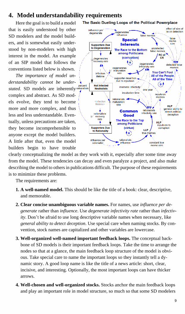
4. Model understandability requirements

Here the goal is to build a model

that is easily understood by other

SD modelers and the model build-

ers, and is somewhat easily under-

stood by non-modelers with high

interest in the model. An example

of an SIP model that follows the

conventions listed below is shown.

The importance of model un-

derstandability cannot be under-

stated. SD models are inherently

complex and abstract. As SD mod-

els evolve, they tend to become

more and more complex, and thus

less and less understandable. Even-

tually, unless precautions are taken,

they become incomprehensible to

anyone except the model builders.

A little after that, even the model

builders begin to have trouble

clearly conceptualizing the model as they work with it, especially after some time away

from the model. These tendencies can decay and even paralyze a project, and also make

describing the model to others in publications difficult. The purpose of these requirements

is to minimize these problems.

The requirements are:

1. A well-named model. This should be like the title of a book: clear, descriptive,

and memorable.

2. Clear concise unambiguous variable names. For names, use influence per de-

generate rather than influence. Use degenerate infectivity rate rather than infectiv-

ity. Don’t be afraid to use long descriptive variable names when necessary, like

general ability to detect deception. Use special care when naming stocks. By con-

vention, stock names are capitalized and other variables are lowercase.

3. Well-organized well-named important feedback loops. The conceptual back-

bone of SD models is their important feedback loops. Take the time to arrange the

nodes so that at a glance, the main feedback loop structure of the model is obvi-

ous. Take special care to name the important loops so they instantly tell a dy-

namic story. A good loop name is like the title of a news article: short, clear,

incisive, and interesting. Optionally, the most important loops can have thicker

arrows.

4. Well-chosen and well-organized stocks. Stocks anchor the main feedback loops

and play an important role in model structure, so much so that some SD modelers

10

feel stocks are the backbone of an SD model, not its main feedback loops. Take

the time to get the structure of your main feedback loops and stocks as clear and

productive as possible.

5. Clearly identified node types. Stocks are boxes. Constants and lookup tables

have dotted arrows. Shadow variables refer to the original variable somewhere

else in the model. These have gray text and brackets (a Vensim convention).

6. Clearly identified node relationship and loop types. Arrows indicate node rela-

tionships. Direct relationships should be solid arrows. Inverse relationships

should be dashed arrows. Important loops should have R or B below the loop

name to indicate a reinforcing or balancing loop. Delays in relationships should

have double slashes. Arrange all arrows so they are easy to follow. Minimize ar-

row crossings.

7. Explanatory notes as needed. For example, the Basic Dueling Loops model

identifies the root cause of change resistance (RC of CR), the low leverage point

(LLP), and two high leverage points (HLP). These are the most important nodes

on the model.

8. Simple easily understood variable equations and units. After adding a new

node to the model, give it a good name and units. Then add the equation as soon

as possible. Careful choice of nodes and arrows will lead to simple variable equa-

tions. These can be so obvious that you don’t have to inspect a need to see its

equation. For example: (1) influence per degenerate x Supporters Due to Degen-

eration = degenerates influence and (2) undetected false memes = false memes –

detected false memes.

Add a node whenever necessary so that your equations are simple and the

model is easily read. For example, instead of A = MAX (B, C + D x (E/F)), add a

node for the C + D x (E/F) calculation. The name of that node will describe what

the calculation using the four variables means. Another node will describe what B

means. Then consider adding a node for the D x (E/F) calculation. Now your

model is much more understandable.

However, for some situations adding nodes would clutter the model. An ex-

ample is the twin nodes degenerates infectivity rate and rationalists infectivity

rate. These share three variables (memetic infectivity, incubation time, and one

year) and have other input variables. By designing the structure as shown, the

model remains uncluttered and readable, at the slight cost of more complex equa-

tions for the twin rates.

Use clear units like births/year. Units must agree with the variable equation

and must be consistent throughout the entire model.

Once a variable has a good name, proper units, and a good simple equation,

it’s self-descriptive. If not, add a comment in the equation editor.

9. Well-designed model pages. Simple models fit on one page. Most models for

difficult problems require multiple pages. These pages should be carefully de-

signed to be subsystems, with the first page having the main model. Large models

will have subsystems of subsystems. Each page should be well named.

11

10. Clearly designed output graphs. Model builders and published model results

will use the output graphs a lot, so they must tell their story well. Use different

colors, line thickness to discriminate between lines. This allows many lines to be

on a single graph without becoming confusing. Use a clear graph title. Make all

graphs consistent.

5. Model validation requirements

5.1. Solving the missing data problem with tendency models

What does the modeler do when key behavior data cannot be or has not been accu-

rately collected? This occurs frequently in soft data like people’s attitude, preferences,

happiness, susceptibility to deception, and so on. It also occurs in problems where certain

data has not been measured, cannot be measured, or is too expensive to collect, like a list

of all proposed solutions to a difficult social problem for the last 50 years and their out-

comes, including whether they were implemented and how much the proposed solution

was changed during implementation. Another example is level of criminal activity in a

population, like income tax evasion and fraud, spouse abuse, and cocaine use. Self-re-

porting, even with face-to-face interviews, is widely known to have low accuracy on be-

havior of this type, making accurate measurement difficult, too expensive, or impossible.

The problem of inability to collect data (both time series and constants) is frequently

solved by estimation. But now when a model is tuned and behavior validation is per-

formed, one is comparing model behavior to estimated data. The model can only be as

good as the estimates. This results in models with low credibility unless the estimates are

provided by experts.

However, estimates from experts are not always available. What does the modeler do

then? Our solution follows that of Aracil (1999), who feels this void can be filled by “the

modern theory of nonlinear dynamical systems. This theory is particularly concerned with

the qualitative aspects of the system’s behavior.” Aracil defines qualitative as “con-

cerned mainly with dynamic tendencies: whether the system is growing, declining, oscil-

lating, or in equilibrium. Qualitative, in this sense, has a fuzzy meaning that covers those

aspects that are less well defined than the strictly quantitative aspects, but which charac-

terize the system’s behavior patterns.”

Since “qualitative” model has a strict definition in the SD literature (it means causal

loop diagrams), we will use the term dynamic “tendency” model. Forrester’s urban decay

model is a tendency model, as it models an idealized representative city and its data is

estimated. All Thwink.org models so far are tendency models and use estimated constants

and lookup tables, and are compared to mostly estimated time series data, since measure-

ment of so many soft factors has never been done. There are exceptions. For example, the

rising ecological footprint serves as a broad measure of growing environmental unsus-

tainability.

Most importantly, tendency models can be used for comparing the relative effective-

ness of different leverage points. Forrester did this by evaluating the relative effectiveness

of the four most popular policies for solving the urban decay problem. The existing SIP

12

analysis does this by measuring the relative amount of leverage in different leverage

points.

5.2. Validation and model types

Validation occurs during model iteration. Homer (1983) defines the term:

“Validation of a system dynamics model can be viewed broadly as a process of

demonstrating that both the structure and behavior of the model correspond to

existing knowledge about the system under investigation.”

Validation centers on the concept of ensuring that the model produces “the right be-

havior for the right reasons.” Here “the right behavior” means model behavior must agree

with real world data to the desired level of accuracy. “The right reasons” means the model

structure produces model behavior for logically sound reasons, as determined by inspec-

tion by model builders and problem experts. Thus, validation is best divided into two

main steps: structure validation and behavior validation. To be through, we have added

a minor third type: technical validation.

The approach to model validation testing depends on to the purpose and type of the

model. If only a general idea of the causal structure is needed, a qualitative causal loop

diagram will suffice. If only the general dynamic tendencies must be understood, a dy-

namic tendency SD model will do. But if exact dynamic behavior must be understood,

then a calibrated SD model is required. A spectrum of model types exists, ranging from

low to high ability to exactly mimic the system of interest, as diagramed below. The latter

two types are quantitative.

Qualitative CLD Models → Dynamic Tendency SD Models → Calibrated SD Models

As a model or model section is constructed, it frequently goes through all three types.

Quick qualitative causal loop diagrams are followed by a tendency SD model, to check

that the dynamic hypotheses of model behave as expected and to begin to explore the

model for insights and unexpected behavior. Some data may be available at this point. If

so, it’s used instead of estimated data. As the model is built, the need for data is clarified,

more data is collected, and the model is tuned to agree with the data to the desired level

of accuracy. This leads to a calibrated SD model, the normal endpoint for most serious

problem-solving SD models.

5.3. Technical validation

This covers technical aspects of SD models that must hold regardless of the structure

or intended behavior of the model. Fortunately, these are few in number. This list assumes

Vensim is the SD modeling tool.

1. Avoid divide by zero. Design constant ranges and lookup table values to avoid

this.

2. No isolated variables or subsystems. All variables must be connected to at least

one other variable. All subsystems must be connected to the main model.

13

3. Run the units check frequently when constructing the model. This checks for

unit consistency between connected nodes, which reduces logical errors.

5.4. Structure validation

Structure validation determines if model behavior arises for “the right reasons.”

Model behavior arises from model structure. In these tests the model is not running, since

we are only inspecting its structure.

These steps must ideally be done by both model builders and problem experts. How-

ever, model builders will perform these steps in more detail. Makes sense means some-

thing makes strong logical and factual sense.

1. Does every node-to-node relationship make sense? This means it must corre-

spond to problem behavior. Constants and lookup tables are included. These must

agree with the real world.

2. Does the arrangement of the stocks make sense? Do they elegantly capture the

behavior of key physical items like housing aging, escalating levels of illicit drug

use, or the progress of proposed solutions?

3. Does every important feedback loop make sense? Do this by walking around

the loop one node at a time and telling a story as you go.

4. Does the feedback loop structure as a whole make sense? Do this by walking

along the causal paths that connect the loops, telling stories as you go.

5. Does the structure of the model strongly support the analysis findings? The

key findings are logically structured as social force diagrams. Does the model

strongly support every node on the diagram and the mode change, except the so-

lutions? Solutions are not in SIP models. Instead, a model contains the leverage

points that solutions push on. It’s possible that large future models may need to

contain some aspects of particular solutions.

6. Is the boundary of the model correct? Exogenous behavior is behavior external

to the model that is included in the model by use of constants and lookup tables.

An SD model’s boundary (what’s inside and outside) is thus defined by its con-

stants and lookup tables.

This test is important for models not developed using root cause analysis,

since the model’s dynamics hypothesis (the key structure) is created intuitively.

It’s not that useful for models developed using root cause analysis, since once the

symptoms node is added to the model as the first node, all other nodes comprise

the causal chain leading to the symptoms. This tends to automatically lead to cor-

rect boundary nodes, since the causal chain nodes (especially the all-important

leverage points) must be variables that change. Everything else must be boundary

nodes.

Many more structure validation tests are discussed in the literature. Those listed above

appear to be the main ones and should suffice for our purposes. More tests will be added

as necessary.

14

5.5. Behavior validation, the correspondence test, and “close enough”

Behavior validation determines if model behavior agrees with real world data to the

desired level of accuracy. During these tests the model is running. The main test is the

correspondence test:

1. Does model behavior correspond closely to collected data? This is the key be-

havior test. The correspondence will never be perfect, since models are simplifi-

cations of reality. Instead, the model should track historical or estimated data to

the desired level of accuracy. In particular, it must agree with the tendency of the

dynamic data, including growth, decline, equilibrium, and oscillation. The model

must also agree with measured constants and lookup tables.

In comparing model behavior to data, how close is close enough? The answer is close

enough to validate that the structure of the model is reasonably correct in terms of the

model’s intended use. For SIP, the intended use is to use high leverage point knowledge

to design solution elements.

If the model passes the “close enough” test, then one may have confidence that vari-

ous leverage point scenarios are reasonably correct. It follows that policies based on these

scenarios can be expected to succeed, within the range of how accurately the model mim-

ics problem behavior for the right reasons, and within the range of confidence gained by

solution element testing.

John Sterman (2000, p. 846) found that “Many modelers focus excessively on repli-

cation of historical data without regard to the appropriateness of underlying assumptions,

robustness, and sensitivity of results to assumptions about the model boundary and feed-

back structure.” In other words, many modelers focus excessively on behavior validation

rather than structure validation. I believe one should focus far more on structure valida-

tion. Behavior validation should be viewed as empirical confirmation that the structure

validation is correct. This is true because it’s easy to build a model that mimics historical

data for the wrong reasons.

Let’s examine an actual SD model to illustrate how close is close enough. This model

was discussed in Jack Homer’s (1983) paper on Partial-model testing as a validation tool

for system dynamics. The paper’s Figures 7 and 10 are shown below.

15

Both graphs contain the same historical time-series data. Note how the data points are

connected with straight lines, giving the historical graph line a rough jagged appearance.

By contrast, the simulated graph line has mostly smooth transitions.

The close match of behavior in Figure 7 was achieved by careful tuning of the model

subsystem that calculated the reporting rate variable, while that subsystem was cut off

from the rest of the model’s behavior to allow partial-model testing. The key tuning as-

pects were use of a third-order delay in rate calculation and a reporting time (a model

constant) of 1.25 years. This resulted in a very good fit. Model oscillation and growth

corresponded surprisingly closely to real world data for a subsystem with only 13 nodes,

including 1 stock, 5 constants, and 2 lookup tables. The subsystem is shown below.

When the subsystem was hooked up to the rest of the model, the result was Figure 10.

Now the simulated curve is not nearly as close to the historical data as it was before. Yet

Figure 10 was acceptable. It was “close enough.” Homer explained that due to the differ-

ence between Figures 7 and 10, one might conclude “that something is wrong with the

model” because the timing of the model’s oscillations is wrong. But “in real life, the

precise timing of the oscillations is sensitive to random disturbances that can affect the

evaluation and reporting process” used in the problem that was modeled.” No model can

predict random event timing precisely. Thus, the behavior validation was close enough.

16

5.6. Behavior validation, additional tests

Here we list behavior tests that have a completely different purpose from correspond-

ence testing. Instead of verifying model behavior accuracy, they look for behavior prob-

lems that indicate structure problems.

2. Extreme condition testing. Does the model exhibit reasonable behavior at a con-

stant’s end points? What if this is done with several constants at the same time?

As you do this, does any unusual behavior offer new insights?

This test is easily run by moving constant sliders to their lower and upper lim-

its. My rule for setting these limits is that they be the limits found in the real

world. These limits are usually estimated. The default value is that of the refer-

ence mode.

3. Sensitivity analysis. This test seeks to determine if model behavior varies in im-

portant unexpected ways when assumptions are varied over their plausible range.

These assumptions can be constants, lookup tables, the level of aggregation used

in stock aging chains, and “even the way people make decisions.” (Sterman 2000,

p. 884)

If a lookup table must be easily tested for different assumptions, it’s usually

possible to add constants controlling the table’s graph, such as its slope, starting,

and ending points, or even all its points. I’ve had to do this only a few times. I’ve

also dragged table graph nodes while the model was running to do simple testing,

as well as tuning.

Commonly only constants are tested dynamically. The other types of assump-

tions are usually tested by inspection. A single constant is easily tested manually

by dragging it slider. Simple testing of multiple constants at a time is frequently

done to test potential weakness one can spot, given the model’s structure. Testing

many constants at a time in a complete manner is so laborious that most SD mod-

eling tools offer automated sensitivity analysis.

However, even with automated testing, complete sensitivity analysis of all

possible constant permutations is impossible, unless the constant ranges are re-

stricted to a small number of discrete values. To solve this problem, Sterman

(2000 italics in the original) recommends that “sensitivity analysis must focus on

those relationships and parameters you suspect are both highly uncertain and

likely to be influential. A parameter around which no uncertainty exists need not

be tested. Likewise, if a parameter has but little effect on the dynamics it need not

be tested….”

Sensitivity analysis is also used to look for what we call high leverage points. Here,

instead of using root cause analysis to find the high leverage points, the modeler assumes

the model already contains the root causes (usually without using that term) and relies on

sensitivity analysis to find the unique combinations of parameter values that would solve

the problem by providing the desired scenario. This approach will not work if the model

does not already contain the root cause. This approach also does nothing to encourage

looking for the root causes.

17

The behavior validation tests described above are sufficient for our purposes for now,

since we are building relatively simple models. More tests will be added if needed.

5.7. SIP leverage point testing

Not listed in the behavior validation tests is testing the behavior of the model’s lever-

age points. This occurs as a normal part of applying SIP. Does this low or high leverage

point behave as expected? Of these two leverage points, which has the highest leverage?

Can pushing on this one high leverage point cause the desired mode change, or must

multiple points be used? And so on. This type of testing is where most testing time goes.

References

Aracil J (1999) On the qualitative properties in system dynamics models. Eur J Econ

Soc Syst 13:1–18. https://doi.org/10.1051/ejess:1999100

Costanza R, Leemans R, Boumans R, Gaddis E (2007) Integrated Global Models. In:

Sustainability or Collapse: An Integrated History and future Of People on Earth. p

417

Forrester JW (1969) Urban Dynamics. The M.I.T. Press

Homer JB (2012) Models that Matter: Selected Writing on System Dynamics from 1985

to 2010. Grapeseed Press

Homer JB (1983) Partial-model testing as a validation tool for system dynamics. In:

Proceedings of the 1983 International System Dynamics Conference. System

Dynamics Society, Chestnut Hill, MA

Meadows D, Meadows D, Randers J, Behrens W (1972) The Limits to Growth.

Universe Books

Sterman J (2000) Business Dynamics: Systems Thinking and Modeling for a Complex

World. McGraw Hill, Boston