Levitating Spinner

Singapore Young Physicist Tournament 2011

RIVER VALLEY HIGH SCHOOL

Category A Group 1

Zhang Nuda

Leung Sin Yung

Lam Teng Foong

2

CONTENTS

Page Number

Nomenclature 3

Introduction 3

Literature Review 4-6

Mathematical Modelling 6-12

Methodology

Phase 1

Phase 2

13-19

Results and Analysis

Phase 1

Phase 2

19-26

Evaluation 27-29

Conclusion 29-30

Appendix 31-33

Bibliography 34

Acknowledgements 34

3

NOMENCLATURE

= moment of inertia of top in z axis (vertical axis)

= moment of inertia of top in x/y axis (horizontal axis)

= effective radius for the moment of inertia of the top

= magnetic field strength

= magnetic field strength at the levitating height of the top

= magnetic field strength in the direction (vertical)

= magnetic dipole moment

= permeability of free space

= angular velocity of the spinning top

= gravitational acceleration, taken to be 9.81

INTRODUCTION

This report investigates the phenomenon in which a hand-spun spinning top

containing a ring magnet is able to levitate above a square piece of magnet, with the

like poles of both magnets facing each other. This phenomenon is demonstrated by

the toy Levitron®, discovered by inventor Roy Harrigan and patented in 1983. In our

experiments we used a similar toy which works on the same principles.

The set consists of a magnetic top (consisting of a permanent ring magnet

enclosed in plastic casing), a plastic lifter plate, and another square permanent

magnet encased in plastic, which acts as the base above which the top levitates.

The square magnet base has a highly uniformed magnetic field, with a region of

weak magnetization in the middle, thus behaving similarly to a ring magnet. The top

is spun on the lifter plate on the magnet base and then lifted to levitation height. If

the top is in alignment with the magnetic field of the base and its mass is within an

4

acceptable range, it will suspend in midair and spin gyroscopically for up to 2

minutes.

Through our experiments, we wish to investigate and analyse the parameters

and conditions governing each successful levitation, and to compare our results with

the mathematical model established previously by Simon, Heflinger and Ridgway[1],

in addition supplement it with our own research findings. This will provide a

comprehensive picture of how the levitating top works, allowing us to determine the

conditions required for it to levitate.

LITERATURE REVIEW

Physics behind the Levitating Top

Since the invention of the Levitron® in 1983, many research papers have

been written to explain the physics behind the magnetic levitating spinner. Two

prominent scientists who have been investigating the Levitron® are Sir Michael Berry

and Andrey Geim, who have both won the Nobel Prize in 2000 for their research in

this area. This toy has sparked the curiosity of physicists for it has overcome certain

theories of magnetic nature that seemingly contradict its ability to levitate, one of

which that is more commonly discussed is Earnshaw‟s theorem.

Earnshaw‟s theorem has proven that it is not possible to achieve stable

levitation of any fixed magnet against gravity. The magnetic moment will attempt to

flip the magnet over. Yet, in the case of the Levitron®, the magnetic spinner is able

to suspend itself while spinning for up to 30 minutes in a vacuum, and a few minutes

outside a vacuum [2]. In this case, the magnetic spinner does not violate Earnshaw‟s

theorem in any way, but instead, gets around it [4]. It is able to maintain stable

levitation while spinning due to a behaviour known as gyroscopic precession, which

causes the top‟s spin axis to turn in a direction at right angles to that in which the

5

torque (magnetic moment) might be expected to turn it[6]. This action in turn aligns

the top‟s precession axis to the direction of the local magnetic field and prevents the

top from flipping. [1] As such, the magnetic field pattern of the base is crucial.

Commercially, the Levitron® and similar products have a strong square magnet base

with a region of weak or null magnetic field in the centre. However a ring magnet with

near zero magnetic field in the centre would also work[1] . As an analogue, the

levitating top can then be seen as being trapped within a well, or a small parameter

space where successful levitation is possible. In our study, we will attempt to define

these parameters governing successful levitation.

Another point to note is the energy system of the whole toy. An object will try

to maintain at the lowest potential energy possible in nature. For an object to remain

in equilibrium, its forces along any axis must add up to zero. Hence, to achieve

stable levitation, there are two conditions that need to be fulfilled. One, the lifting

force must balance the weight of the top so that the top levitates at a constant height,

and second, the potential energy at the point of levitation must be at the minimum.[1]

Methods to Define “Conditions”

Various sources have provided us with a range of angular velocities of the top

for which it can hover successfully. According to Fascinations®, the maker of the

Levitron®, the top would be stable when spinning at 20 to 35 revolutions per second

(approx. 125 - 220 rads-1), becoming unstable above 35 to 40rps (approx. 220 –

251rads-1) and below 18rps (approx. 113rads-1) [2]. This is very similar to the results

obtained by the experiments of Simon, Heflinger and Ridgway, showing an upper

frequency limit of 254rads-1 and a lower frequency limit of 114rads-1 [1]. As the

precession frequency is inversely proportional to the spin frequency, if the angular

velocity of the top exceeds the upper spin limit, the precession frequency will be

6

insufficient in keeping the top oriented to the local magnetic field direction and the

top falls, thus originates the upper spin limit. On the other hand, beyond the low

frequency limit, the angle of precession of the top is too great such that the magnetic

field gradient can no longer support it and it falls [1].

Fascinations® also states that the mass of the top is critical for the top to

successfully levitate as it determines the “equilibrium height” where the magnetic

force balances the force of gravity [2]. The stable range of this “equilibrium height” is

small and hence adjusting the top‟s mass with washers is often required for the top

to levitate.

Therefore, we can conclude that we have the following conditions we can investigate:

Range of angular velocity required for levitation

Range of precession frequency required for levitation

Range of mass of the top required for levitation

Range of levitating height required for levitation

MATHEMATICAL MODELLING

As mathematical models of the levitating top have already been published in

scientific journals, we would like to use them as our foundation to find the conditions

of which our top would levitate. One paper from which we will largely draw the basis

of our investigation from is Spin Stabilised Magnetic Levitation by M.D. Simon, L.O.

Heflinger and S.L. Ridgway[1].

1) Mathematical model to calculate the largest possible mass of top

[1] states that the potential energy of the levitating top is defined as:

(1)

7

Where,

U is the potential energy of the top

is the magnetic dipole moment of the top

B is the magnetic field strength of the magnetic base at the centre of gravity at the

levitating point

m is the mass of the top

g is the acceleration due to gravity

z is the displacement of the centre of gravity of the top in the z direction (vertical)

from the point of reference ( in this case the top surface of the base plate magnet)

This equation can be expanded into

(2)

Utilising the curl and divergence equations and , the

magnetic field in the r and z direction around the levitation can be expressed as a set

of power series equations

(3)

(4)

where

8

and

Using the equations from [1], by substituting (3) and (4) into (2) as well as

ignoring terms larger than the 4th order, this gives us the following approximation

(5)

The report states that in order for the potential energy of the top to be stable

during levitation, equation (5) must be quadratic in both z and r directions to

resemble the shape of a potential energy well.

One of the requirements needed to satisfy the above condition is

(6)

which can be expressed as

(7)

Assuming values g and are constants, the magnetic field gradient in the z

direction,

, is inversely proportional to the mass of the levitating top. Therefore,

the point on the graph at which

is the lowest is also when the top with the

greatest possible mass can be levitated.

Hence, the equation to calculate the maximum mass of the top for it to

achieve levitation is

9

(8)

On the other hand, since

is a function of z, if is a known value, then

it can be used to calculate the highest possible height the top can levitate above the

magnetic base plate, , since

(9)

Where is the distance between the centre of gravity and the lowest point of the

top in the z direction at that instant.

2) Mathematical model to calculate the range of angular velocity for which

the top will levitate

[1] states that the angular velocity of the top, , can be defined as

(10)

Where,

is the moment of inertia along the z axis

is the moment of inertia along the x and y axis

is the effective radius for the moment of inertia

Also, can be expressed in terms of m and as

(11)

10

By substituting (11) into (10), the range of angular velocity can be simplified to

become

(12)

Hence, by finding the values , B, , and m and substituting them into (25), we

can calculate the range of that when achieved by the top will allow it to achieve

levitation.

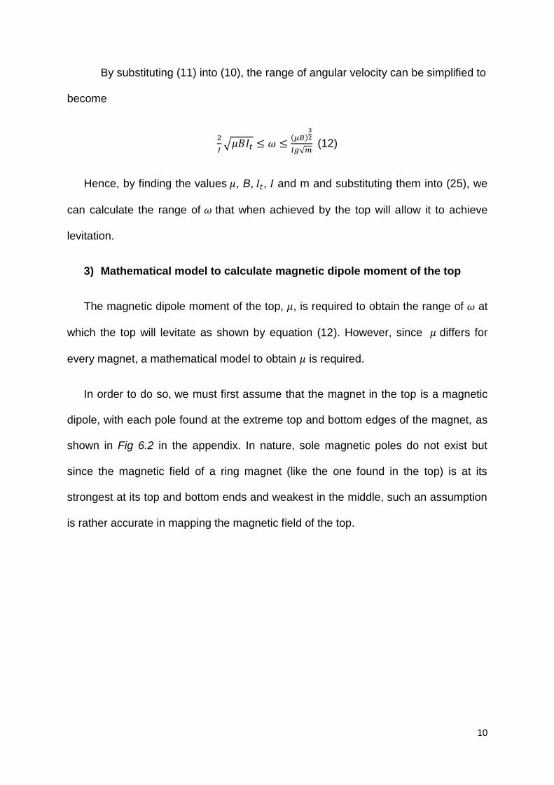
3) Mathematical model to calculate magnetic dipole moment of the top

The magnetic dipole moment of the top, , is required to obtain the range of at

which the top will levitate as shown by equation (12). However, since differs for

every magnet, a mathematical model to obtain is required.

In order to do so, we must first assume that the magnet in the top is a magnetic

dipole, with each pole found at the extreme top and bottom edges of the magnet, as

shown in Fig 6.2 in the appendix. In nature, sole magnetic poles do not exist but

since the magnetic field of a ring magnet (like the one found in the top) is at its

strongest at its top and bottom ends and weakest in the middle, such an assumption

is rather accurate in mapping the magnetic field of the top.

11

Figure 1

By taking this assumption into consideration, the magnetic field strength of the

top at point “a” (shown in the Fig 1), , can be expressed as the following equation

(13)

where

is the permeability of free space

is the “pole strength” of each pole

This equation can be simplified into

(14)

The magnetic dipole magnet of a magnet is conventionally defined as

12

(15)

Where is the vector separating the two opposite poles, which in our case can

be defined as

(16)

By substituting (16) into (14), we now get

(17)

Rearranging the terms gives us the linear equation

(18)

where

Hence, with values and d as constants, by measuring how varies with z

and plotting a graph of

against z, we will be able to obtain the value of ,

which is the gradient of the linear equation.

13

METHODOLOGY

To understand the phenomenon of the levitating top, we conducted

experiments that allow us to collect our own set of experimental data, and, with some

analysis, account for the various parameters that govern a successful levitation. This

will allow us to prove that the existing conclusions made by other research papers

are valid, and in addition better define those parameters with our own findings to

provide a more comprehensive picture of the phenomenon.

There are two phases in the experimental stage of our investigation.

Phase 1 is to find values and which are required by equations (8) and (12)

to obtain the largest possible weight of the top and the range of angular velocity at

which the top will levitate.

Phase 1 includes two experiments:

1. Experiment 1.1: Investigate of how varies with z

2. Experiment 1.2: Obtain value

Phase 2 involves experiments that tests the validity of the range of and

value obtained by equations

and

respectively.

Phase 2 includes two experiments as well:

1. Experiment 2.1: Compare range of obtained by

to

range of obtained in reality

14

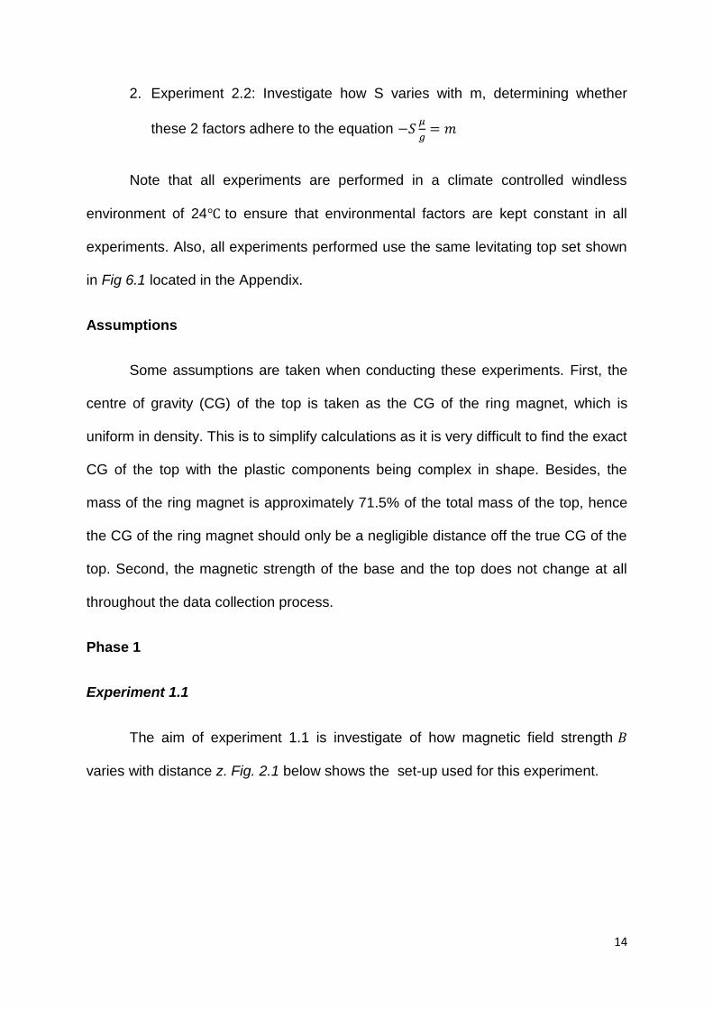
2. Experiment 2.2: Investigate how S varies with m, determining whether

these 2 factors adhere to the equation

Note that all experiments are performed in a climate controlled windless

environment of 24 to ensure that environmental factors are kept constant in all

experiments. Also, all experiments performed use the same levitating top set shown

in Fig 6.1 located in the Appendix.

Assumptions

Some assumptions are taken when conducting these experiments. First, the

centre of gravity (CG) of the top is taken as the CG of the ring magnet, which is

uniform in density. This is to simplify calculations as it is very difficult to find the exact

CG of the top with the plastic components being complex in shape. Besides, the

mass of the ring magnet is approximately 71.5% of the total mass of the top, hence

the CG of the ring magnet should only be a negligible distance off the true CG of the

top. Second, the magnetic strength of the base and the top does not change at all

throughout the data collection process.

Phase 1

Experiment 1.1

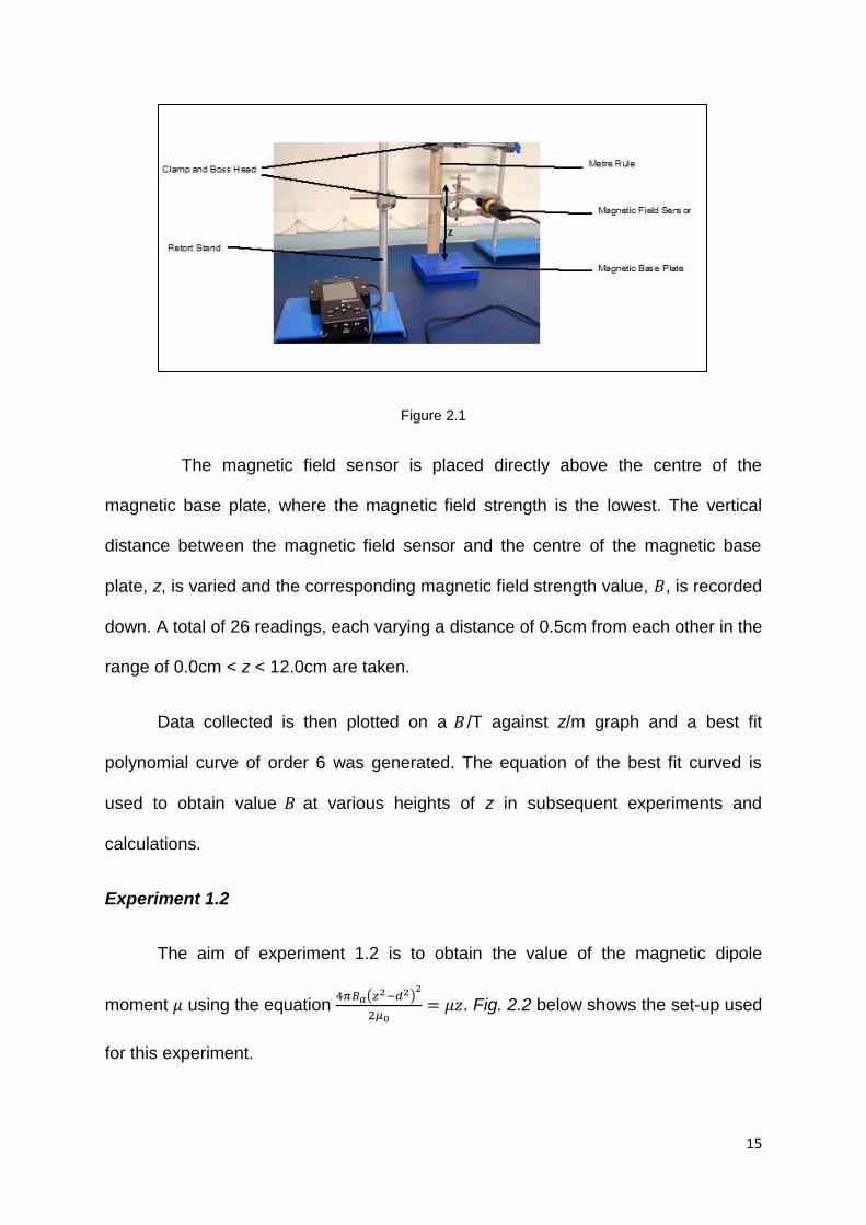
The aim of experiment 1.1 is investigate of how magnetic field strength

varies with distance z. Fig. 2.1 below shows the set-up used for this experiment.

15

Figure 2.1

The magnetic field sensor is placed directly above the centre of the

magnetic base plate, where the magnetic field strength is the lowest. The vertical

distance between the magnetic field sensor and the centre of the magnetic base

plate, z, is varied and the corresponding magnetic field strength value, , is recorded

down. A total of 26 readings, each varying a distance of 0.5cm from each other in the

range of 0.0cm < z < 12.0cm are taken.

Data collected is then plotted on a /T against z/m graph and a best fit

polynomial curve of order 6 was generated. The equation of the best fit curved is

used to obtain value at various heights of z in subsequent experiments and

calculations.

Experiment 1.2

The aim of experiment 1.2 is to obtain the value of the magnetic dipole

moment using the equation

. Fig. 2.2 below shows the set-up used

for this experiment.

16

Figure 2.2

Figure 2.3

The magnetic sensor is placed directly above the centre of the top. The top is

held upside down in a fixed position by a clamp. The distance h (Fig. 2.3), is varied

by moving the position of the magnetic sensor vertically and the corresponding

magnetic field strength value, , is recorded down. A total of 20 readings of ,

each varying a distance of 0.5cm from each other between 1.0cm < h< 10.0cm are

taken. Value z is obtained by subtracting 0.39cm from the values of h. A graph of

/ against z/m is plotted where d=0.25cm. A best fit line is generated

and the gradient of the line is deemed as the value .

17

Phase 2

Experiment 2.1

The aim of experiment 2.1 is to compare the range of the angular velocity

of the levitating top obtained by

to range of obtained in

reality. Fig 3.1, 3.2 and 3.3 below show the set-up used for this experiment.

Figure 3.1

Figure 3.2 Figure 3.3

18

Two Casio Exilim EX-FH100 cameras are positioned as shown in Fig 3.1

above, held in fixed positions by two tripod stands. Each successful levitation,

defined as one that spins for over 1 minute and falls straight down instread of

slipping sideways once it exists stable levitation, is recorded from the top and side

view by the two cameras at 240fps.

The videos are then analysed using the Tracker software by Douglas Brown.

Video footage from camera 1 is used to determine the levitation height of the

top, L, measured from the surface of the base to the base of the top. A total of 3

videos were analysed. A distance of 0.85cm, ( term found in (9)) the distance from

the lowest point of the top to the Centre of Gravity (CG) of the ring magnet, is

added each value of L to obtain z and then the average <z>, which will be

substituted into the best fit curve generated in experiment 1.1 to obtain a

corresponding value of to be used in subsequent calculations.

Video footage from camera 2 is used to obtain the the top‟s angular velocity 5

seconds into levitation and 5 seconds before the end of levitation. A total of 10

videos were analysed to obtain < >and < > respectively which will be

compared to the range of obtained using the equation

.

Experiment 2.2

The aim of experiment 2.2 is to investigate how S varies with m, determining

whether these 2 factors adhere to the equation

mentioned in the

mathematical modelling. A similar set-up used in experiment 2.1 is used for

experiment 2.2, except that only footage from camera 1 is used.

19

The mass of the top is increased by adding Blu Tac at 0.002g intervals till 6

sets of data are obtained. Each set of data comprises of 3 successful levitations at

that particular mass. The average levitating height of the top at each different mass,

<L>, is obtained and used to obtain value <z> like in experiment 2.0. Values of <z>

are then compared to the ones generated by

to access the validity of the

equation.

RESULTS AND ANALYSIS

Phase 1

Experiment 1.1

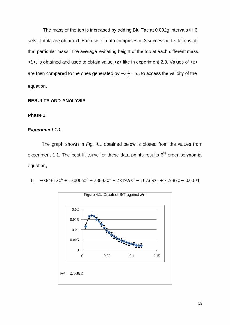
The graph shown in Fig. 4.1 obtained below is plotted from the values from

experiment 1.1. The best fit curve for these data points results 6th order polynomial

equation,

Figure 4.1: Graph of B/T against z/m

R² = 0.9992

0

0.005

0.01

0.015

0.02

0 0.05 0.1 0.15

20

This curve generated could be used to find the magnetic field strength, B and

magnetic field strength gradient, , at the point where the top levitates, L.

Using results of <L> from experiment 2.1, equation (9), and measuring

=0.85cm we are able to obtain the value z

This value of z is then substituted into the equation of best fit curve in

experiment 1.1 to obtain value B which is required in subsequent calculations

To obtain , the equation of the best fit curve is differentiated and its first

derivative is obtained. Fig 4.2 below shows the graph of S/ against z/m

Figure 4.2: Graph of S/ against z/m

21

NOTE: For Fig 4.2 the extrapolation of the graph beyond approximately z=0.1m could be ignored as is beyond the experimental

data we obtained.

The turning point where

shows the

coordinates . This goes to show that the maximum height

of levitation of the top from the base is 0.0354m, equivalent to 3.54cm. At the same

we have obtained .

Furthermore, we can also use the first derivative of the best fit curve as a way

to define S in terms of z, which will be required in the analysis of results of

experiment 2.2.

The equation for the first derivative is

Experiment 1.2

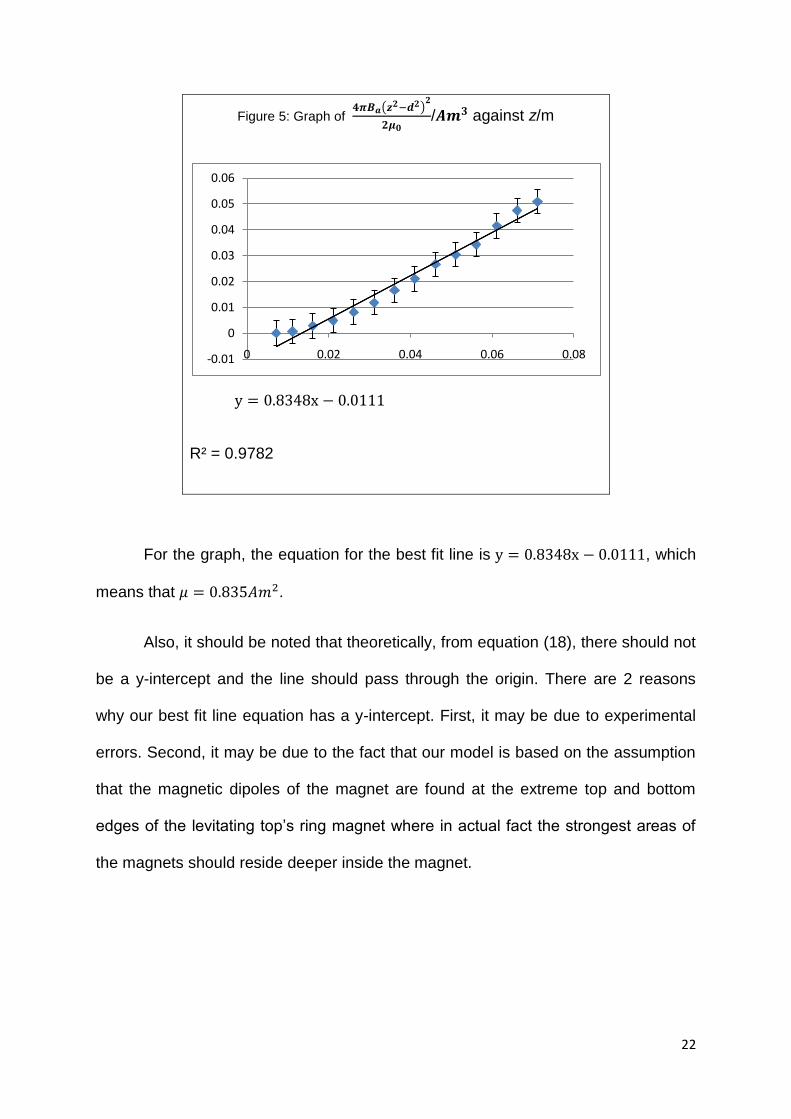
Fig 5 shows the results of experiment 1.2 plotted in a graph of

/ against z/m with a best fit line generated.

As shown by equation (18), values

and z have a linear

relationship with each other and the gradient of these 2 variables is the value ,

which is what we want to obtain from the results in this experiment.

22

Figure 5: Graph of

/ against z/m

R² = 0.9782

For the graph, the equation for the best fit line is , which

means that .

Also, it should be noted that theoretically, from equation (18), there should not

be a y-intercept and the line should pass through the origin. There are 2 reasons

why our best fit line equation has a y-intercept. First, it may be due to experimental

errors. Second, it may be due to the fact that our model is based on the assumption

that the magnetic dipoles of the magnet are found at the extreme top and bottom

edges of the levitating top‟s ring magnet where in actual fact the strongest areas of

the magnets should reside deeper inside the magnet.

-0.01

0

0.01

0.02

0.03

0.04

0.05

0.06

0 0.02 0.04 0.06 0.08

23

Phase 1 Conclusion

From phase 1 and previous calculations, we have obtained the following

values

.

(See appendix for calculations)

(See appendix for calculations)

(Obtained in experiment 2.1)

With these values, we can now use equations (8) and (12) to obtain the

largest possible weight of the top and the range of angular velocity at which the top

will levitate.

For the largest possible weight

For the range of angular velocity required to levitate

24

The range of angular velocity obtained,

is rather close to the range established by [1], between 114rads-1 and

254rads-1, and by [2], 20 to 35 revolutions per second (approx. 125 - 220 rads-1). The

higher than usual upper angular velocity limit from our calculations compared to

those of published sources may be due to the fact that our values are based on the

magnetic levitating top set we are using, which may be of a different brand and type

from the one used by the published sources. Other reasons might include

experimental error and less accurate calculations (such as the calculation of and )

which may cause our results to be less accurate.

Phase 2

Experiment 2.1

Table 1 below shows the angular velocity of the top 5 seconds into levitation

and 5 seconds before exiting stable levitation. All values recorded fall within our

calculated angular velocity range.

Table 1

Trials 5s into

levitation

5s before exiting stable

levitation

1 146 119

2 148 129

3 156 121

4 181 119

5 171 119

25

6 171 121

7 171 116

8 162 116

9 162 118

10 168 119

Average 163 120

For the angular velocities recorded 5 seconds into levitation, the angular

velocity tends to vary over a range, but still falls within 145< <181 . This

might be the case as the initial force used to spin the top varies for each trial as it is

done by hand in our experiments. The limits to how fast a human can spin is also

much lower than that of machinery or other methods used in more sophisticated

methods, for example, the one mentioned in [1]. Hence, our results cannot conclude

whether our upper angular velocity limit calculated in phase 1 is accurate as we are

unable to make the top spin at such high velocities.

For the angular velocities recorded 5 seconds before the top exits stable

levitation, the results fall rather close to the lower angular velocity limit calculated in

phase 1, with only a difference of 16 between the calculated value and the

average of the 10 trials. The slightly higher experimental values may be because the

readings are taken 5 seconds before the top exits stable levitation and not at the

exact instant when the top becomes unstable. Therefore, it is understandable that

the experimental results are slightly higher than expected as the top will continue to

decelerate for 5 seconds after the readings are taken. Therefore it is possible to

conclude that the mathematical model we used to obtain the lower angular velocity

limit is rather accurate in finding the lowest angular velocity required by the top to

achieve levitation.

26

Experiment 2.2

Table 2 shows the results from experiments 2.2. As previously done in

experiment 1.1, <L> is converted to using equation (9). Values

are then compared to the z values obtained using equation (6),

, known as

values . It is possible for (6) to produce values because S is

expressed in terms of z by the first derivative of the best fit curve in experiment 1.1.

Table 2: Average height of top from base with varying masses

m/kg

L/mm z/mm

L1 L2 L3 <L> % Difference

Percentage

difference

0.02340 21.13 18.62 20.58 20.11 28.68 28.87 -0.6236%

0.02342 22.86 19.14 23.70 21.90 30.47 28.88 5.508%

0.02344 23.35 21.64 21.58 22.19 30.76 28.90 6.442%

0.02346 26.61 25.28 23.85 25.25 33.82 28.92 16.94%

0.02348 26.53 26.23 26.24 26.33 34.90 28.94 20.62%

0.02350 25.17 26.58 26.17 25.97 34.55 28.96 19.30%

By comparing and it can be seen that (6) is rather

accurate in portraying the relationship between m and S, with the largest percentage

difference between and only at approximately 20%.

From this we can also conclude that equation (8), which is derived from (6), is

also accurate in calculating . This makes our calculated value of at 26.6g

using equation (8) a valid estimation for the largest possible mass of a top for it to

levitate.

27

EVALUATION

Phase 1 Experiments

In Phase 1, the readings of the magnetic field strength measured with the

Addestation magnetic sensor tends to fluctuate. This might be due to the magnetic

field not being aligned perpendicularly with the sensor. If the magnetic field „passes‟

through the sensor at an angle, the value measured will be lower than the actual

value of the magnetic field at the measured point. To minimise this error, the sensor

is manipulated at the point of measurement by tilting it slightly in different directions

until the highest possible value is measured. A tripod stand with a clamp is also used

to hold the sensor in place each time we take the measurement.

Also, as the base of the tripod stand is metallic (magnetic), it might serve as a

source of interference for the measurement of the magnetic strength of the base

magnet and top. Attempts to reduce these interference includes placing the base as

far from the base or top as possible using clamps and rods made of non-magnetic

materials, as seen in Fig. 3.2 and 3.3.

Even with the above precautions, fluctuations in the reading during each

measurement cannot be totally avoided. To account for such fluctuations, the

percentage error of each set of data is calculated. For example, when the magnetic

sensor is at a height, m in experiment 1.1, the percentage error is:

Closer to the spot where the magnetic field strength is the maximum, there

are larger fluctuations. For example, at , the percentage error

obtained is as follows:

28

This large percentage error remains for , and other regions

with a high value of magnetic flux density (measured in Gauss) taken. This might

possibly be due to the non-uniform magnetic field in the region.

Phase 2 Experiments

For Phase 2 Experiments, interference from external surroundings while

obtaining experimental data is minimized by conducting the experiment in a

controlled environment with minimal winds and using tripod stand made of non-

magnetic materials. However, due to the limitations of our equipments some factors

are not easily controlled, such as the initial angular velocity of the magnetic levitating

top. Some fluctuation is inevitable as the initial force used to spin the top by hand

cannot be precisely controlled and will vary with every spin. As a result, the initial

angular velocity of the spin varies across a range of values (150±10 rad s-1 ).

There are also limits to the maximum speed at which a human hand can spin

the top, which are much lower than those achievable by more sophisticated methods,

such using a synchronous magnetic drive[1] to control spin rate. Hence it is not

possible to obtain and test the maximum angular velocity of the top (254rads-1 [1]),

which is beyond the ability of the human hand.

Another source of error arises from the limitations of the Tracker software

used for the video analysis. The software relies on individual human judgement in

the analysis of each footage. This renders the analysis prone to human biasness,

possibly resulting in the readings being precise but not accurate, as in our case

where each video is only analysed by one person. Further improvements could be

29

made in the future with a few people analysing each of the videos and conducting

inter-rater reliability tests to minimize or remove any individual biasness.

Lastly, the use values of the moment of inertia of the top and is only an

approximation and the values are not accurate, due to the dimensions of the top

being simplified for easier calculations. This is largely due to the non-uniform shape

of the plastic parts of the top. However, the effect of this approximation is not too

significant as majority of the mass of the top is due to the ring magnet in the middle,

which has a uniform disc shape, and hence its inertia could be calculated easily and

accurately.

CONCLUSIONS

An experimental study was conducted on the phenomenon of the levitating

magnetic spinner, defining the parameters in which the toy can achieve stable

levitation, based on previous research by Simon, Heflinger and Ridgway

In our study, the calculated angular velocity of the top required for stable

levitation is , while the actual velocity collected in our

experiments is . Discrepancies between the

theoretical range of angular velocities and the actual range are attributed largely to

human limitations and also, to a smaller extent, the limitations in the equipments

available. In addition, we have theoretically determined the maximum mass of the

top at which it can successfully levitate (26.6g), which is done by equating the

maximum weight of the top to the maximum magnetic field gradient, and the

maximum height at which the top can levitate (3.54cm) Also, we have established a

relationship between the mass of the top and its levitation height.

30

Even so, more detailed and vigorous testing using better laboratory

equipment will be required to test the true validity of equations

and

, especially for the mathematical model of the upper

angular velocity limit of which the results from our experiment are unable to conclude

its accuracy.

Therefore, our investigation has shown the conditions required for our top, or

any other magnetic levitating spinner, to levitate. These boundaries similar to the

boundaries set by the paper by M.D. Simon, L.O. Heflinger and S.L. Ridgway[1]. By

supplementing previous research with our own findings, have better defined the

boundaries in which the levitating spinner works, providing a more comprehensive

picture of this intriguing phenomenon. This can also serve as a base for future

research, which could delve even deeper into this phenomenon by taking into

account factors such as the gyroscopic precession, which we have failed to cover in

our investigation.

31

APPENDIX

Figure 6.1 Picture of the Hi-Tech Permanent Magnetic Suspensible Flying Disk

Figure 6.2: Cross section of top and base

Moment of Inertia of the Top

Figure 7.1: Generalised cross-sectional diagram of the top (not drawn to scale)

(To aid in calculations, certain insignificant details and features of the top are ignored).

32

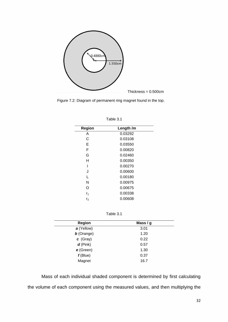
Thickness = 0.500cm

Figure 7.2: Diagram of permanent ring magnet found in the top.

Table 3.1

Region Length /m

A 0.03292

C 0.03108

E 0.03550

F 0.00820

G 0.02460

H 0.00350

I 0.00270

J 0.00600

L 0.00180

N 0.00975

O 0.00675

r1 0.00338

r2 0.00608

Table 3.1

Region Mass / g

a (Yellow) 3.01

b (Orange) 1.20

c (Gray) 0.22

d (Pink) 0.57

e (Green) 1.30

f (Blue) 0.37

Magnet 16.7

Mass of each individual shaded component is determined by first calculating

the volume of each component using the measured values, and then multiplying the

33

total mass of the top (23.4g) with the ratio of the volume of each component to the

total volume of the top.

In the following calculations, denotes the moment of inertia in the z axis

(vertical axis), while denotes the moment of inertia in the x/y axis (horizontal axis).

(3 s.f.)

(3 s.f.)

34

BIBLIOGRAPHY

[1] Simon, M.D., Heflinger, L.O. & Ridgway, S.L. (1997). Spin stabilized magnetic levitation. American Journal of Physics, 65(4), 286-292.

[2] The PHYSICS of Levitron. Retrieved 10 November, 2010, from http://www.levitron.com/physics.html

[3] Berry, M.V. (1996). The LevitronTM: an adiabatic trap for spins. Proc. Roy Soc. Lond. A, 452, 1207-1220

[4] Gibbs, P. & Geim, A (1997, March 18) Is Magnetic Levitation Possible? Retrieved 10 November, 2010, from http://www.ru.nl/hfml/research/levitation/diamagnetic/levitation_possible/

[5] McBride, J. M.(2001, August 27) A Toy Story. The Chemical Relevance of Earnshaw's Theorem, and How the Levitron® Circumvents It. Retrieved 10 November, 2010, from http://www.chem.yale.edu/~chem125/levitron/levitron.html

[6] Precession of Top. Retrieved 11 November, 2010, from http://hyperphysics.phy-astr.gsu.edu/hbase/top.html

[7] Gyroscopes—Everything you need to know. Retrieved 11 November, 2010, from http://www.gyroscopes.org/behaviour.asp

[8] Tracker Video Analysis and Modelling Tool for Physics Education. Retrieved October 28, 2010, from http://www.cabrillo.edu/~dbrown/tracker/

ACKNOLEDGEMENTS

We would like to thank River Valley High School for providing us with the

opportunity and the resources to undergo this investigation. We would also like to

thank our teachers-in-charge, Mr Lee Tat Leong and Mr Teo Tai Wei for their

guidance and support during this competition, and lastly the authors of [1] as much

of our ideas are based on their research paper.