Synthetic ECG Generation and Bayesian Filtering Using …lcp.mit.edu/pdf/SayadiPM10.pdf · 1...

1 Accepted to the journal of Physiological Measurement for future publication (30 June 2010).

Synthetic ECG Generation and Bayesian Filtering Using a Gaussian Wave-Based Dynamical Model

Omid Sayadi1, Mohammad B. Shamsollahi

1, and Gari D. Clifford

2

Biomedical Signal and Image Processing Laboratory (BiSIPL), School of Electrical Engineering, Sharif University of Technology, Tehran, Iran.

1

Institute of Biomedical Engineering, Department of Engineering Science, University of Oxford, UK. 2

Email: [email protected], [email protected], [email protected]

Abstract In this paper, we describe a Gaussian wave-based state space to model the temporal dynamics of electrocardiogram (ECG) signals. It is shown that this model may be effectively used for generating synthetic ECGs as well as separate characteristic waves (CWs) such as the atrial and ventricular complexes. The model uses separate state variables for each CW, i.e. P, QRS and T, and hence is capable of generating individual synthetic CWs as well as realistic ECG signals. The model is therefore useful for generating arrhythmias. Simulations of sinus bradycardia, sinus tachycardia, ventricular flutter, atrial fibrillation, and ventricular tachycardia are presented. In addition, discrete versions of the equations are presented for a model-based Bayesian framework for denoising. This framework, together with an extended Kalman filter (EKF) and extended Kalman smoother (EKS), were used for denoising the ECG for both normal rhythms and arrhythmias. For evaluating the denoising performance the signal-to-noise ratio (SNR) improvement of the filter outputs and clinical parameter stability were studied. The results demonstrate superiority over a wide range of input SNRs, achieving a maximum 12.7 dB improvement. Results indicate that preventing clinically relevant distortion of the ECG is sensitive to the number of model parameters. Models are presented which do not exhibit such distortions. The approach presented in this paper may therefore serve as an effective framework for synthetic ECG generation and model-based filtering of noisy ECG recordings. Keywords: denoising, electrocardiogram (ECG), ECG modeling, extended Kalman filter (EKF), extended Kalman smoother (EKS).

1. Introduction The electrocardiogram (ECG) obtained by a noninvasive technique is a record of the bio-potentials associated with the contractions of the heart muscle, which provides useful information for the detection, diagnosis and treatment of cardiac diseases. However, ECG signals are usually corrupted with unwanted interference, generally referred to as noise or artifact. Since the interference is often in-band, time-coincident and morphologically similar to cardiac activity, accurately extraction of information from an ECG requires effective characterization of the constituent waveform morphologies. Any filtering technique must preserve the important clinical features while providing high attenuation of noise. Accordingly, several techniques have been proposed to extract the ECG components contaminated with the background noise and allow the measurement of subtle features in the ECG signal. The adaptive filter architecture is among the common approaches (Thakor and Zhu

mailto:[email protected]�


1991). Statistical techniques such as principal component analysis (Moody and Mark 1989), independent component analysis (Barros et al. 1998, and He et al. 2006), and neural networks (Clifford and Tarassenko 2001) have also been used to extract a noise-free signal from the noisy ECG. Over the past several years; methods based on the wavelet transform (WT) have also received a great deal of attention for the denoising of signals that possess multi-resolution characteristics such as the ECG (Kestler et al. 1998, Donoho 1995, Popescu et al. 1998, Daqrouq 2005, Sayadi and Shamsollahi 2007).

In order to test the performance of a filtering system there are generally two approaches. The first is to use expert annotated data. Although this guarantees that the data are realistic, it is hard to test at extremely low noise levels, or when the data are swamped by high noise. To test in such circumstances one must employ a realistic model of the ECG. Although some excellent cellular models exist, such approaches are computationally intensive and therefore difficult to employ for large-scale simulations. McSharry et al. (2003) presented an electrocardiographic dynamical model (EDM) for generating a synthetic ECG signal with realistic PQRST morphology and heart rate dynamics. The aim of this model was to provide a standard realistic ECG signal with known characteristics, which can be generated with specific statistics thereby facilitating the performance evaluation of a given technique. Synthetic ECGs can be generated with different sampling frequencies, morphologies, heart rates, heart rate variabilities (HRVs) and different noise levels.

Many updates to this model and applications of it have been made over the last ten years since its first creation in 2000. First, a model-based filtering, compression and segmentation/feature extraction approach based on a least squares fit of observations to the model was proposed (Clifford et al. 2005). This approach was then applied to filtering, compression, QT-interval analysis and beat segmentation (Clifford and Villarroel 2006). The model has also been used to model fetal ECG (Sameni et al. 2007a). Recently, the model was updated to include a Hidden Markov Model to account for beat type changes (Clifford et al. 2008, Clifford et al. 2010). Moreover, in a recent work, we have provided a modified version of the EDM on a wave-related basis, which showed promising results for PVC detection (Sayadi et al. 2010).

Since the model formulation was in the form of a state space representation, Bayesian estimation procedures could be applied to the model, if appropriate observations were found and related to the state variables. In a pioneer work, Sameni et al. proposed the use of an explicit phase variable instead of the first two motion variables that indicates the angular location of the P, Q, R, S, and T waves. They obtained a compact set with two state variables, based on which the ECG measurement and the constructed phase signal could be relate to the state variables of the state space equations. Bayesian model-based frameworks were also proposed where the model was updated to explicitly use the three orthogonal dimensions and the equations were re-factored into a polar coordinate system to denoise the ECG by using a Kalman filter to track and constrain the model parameters (Sameni et al. 2006, Sameni et al. 2007b). This model has also been used to remove cardiac contaminants (Sameni et al. 2008). In addition, this technique has been modified using auto-regressive dynamics assignment to the model parameters (Sayadi et al. 2007) and applied to simultaneous denoising and compression (Sayadi and Shamsollahi 2008), and ECG beat segmentation (Sayadi and Shamsollahi 2009).

In the previously proposed approaches towards Bayesian ECG analysis (Sameni et al. 2007b, Sayadi and Shamsollahi 2008), occasional morphologic changes that only appear in some of the ECG cycles has considerable effects on the filter performance. In these cases, the phase error of the model can lead to large errors in the Gaussian parameters, since neither the model nor the measurements are reliable for the filter. For such occasional morphologic changes, even temporal adaptation of the filter parameters is not helpful, as the filter does not have sufficient time to adapt itself.


In this paper, in order to overcome such inaccuracies, we assume the presence of distinct coupled components for the ECG signal, based on which a Gaussian wave-based dynamical framework is developed. We study the proposed wave-based ECG dynamical model as a generative model for producing synthetic ECG signals as well as separate characteristic waveforms (CWs) such as the P-wave in isolation. In this way we simulate a series of arrhythmias with the model. In addition we investigate the state space Bayesian filtering approach (using our model with the EKF and EKS) and evaluate their performance on both normal and ectopic beats.

The paper is organized as follows. Section 2 provides relevant background on the original ECG dynamical model and presents the wave-based dynamical model. In Section 3, the details of the proposed method for synthetic ECG generation and Bayesian denoising is presented. Section 4 is devoted to simulation results. Finally, discussion and concluding remarks are provided in section 5.

2. ECG Dynamical Model In this section, the original ECG dynamical model proposed by McSharry et al. (2003) is reviewed briefly. The model is later used to introduce the wave-based dynamical model by modifications in the ECG formation using the characteristic waves. In addition, the resultant model is shown to be capable of generating separate CWs as well as the synthetic ECG. 2.1. Original Dynamical Model McSharry et al. (2003) proposed a realistic synthetic ECG generator using a set of state equations that generates a three-dimensional (3D) trajectory in a 3D state space with coordinates (x, y, z). The model consists of a circular limit cycle of unit radius in the (x, y) plane around which the trajectory is pushed up and down as it approaches the turning points in the ECG (P, Q, R, S and T). In fact, the characteristic waveforms of the ECG are described by Gaussian-type events corresponding to negative and positive attractors/repellors in the z direction. Quasi-periodicity of the ECG is reflected by the movement of the trajectory around the attracting limit cycle, while the inter-beat variation in the ECG is reproduced using the motion of the trajectory in the z direction. The original dynamical equations of motion are given by a set of three ordinary differential equations in Cartesian coordinates:

⎩⎪⎨

⎪⎧

)(2

exp 0},,,,{

2

2zz

baz

xyyyxx

TSRQPi i

iii −−

∆−∆−=

+=−=

∑∈

θθ

ωγωγ

�

(1)

where 221 yx +−=γ , πθθθ 2mod)( ii −=∆ , ),(2 xyanat=θ is the four quadrant arctangent of the

elements of x and y, ranging over ],[ ππ− , and ω is the angular velocity of the trajectory as it moves around the limit cycle, and is related to the beat-to-beat heart rate as ω=2πf. As it is seen in (1), each of the P, Q, R, S, and T-waves of the ECG waveform are modeled with a Gaussian function located at specific angular positions θ i. The ai, bi and θ i terms in (1) correspond to the amplitude, width, and center parameters of the Gaussian terms of this equation. Finally, the baseline wander of the ECG is modeled with the parameter z0 that is assumed to be a relatively low amplitude sinusoidal component coupled with the respiratory frequency (McSharry et al. 2003). The z coordinate of this trajectory, when plotted versus time gives the synthetic ECG. It can be seen that the ECG signal z is represented


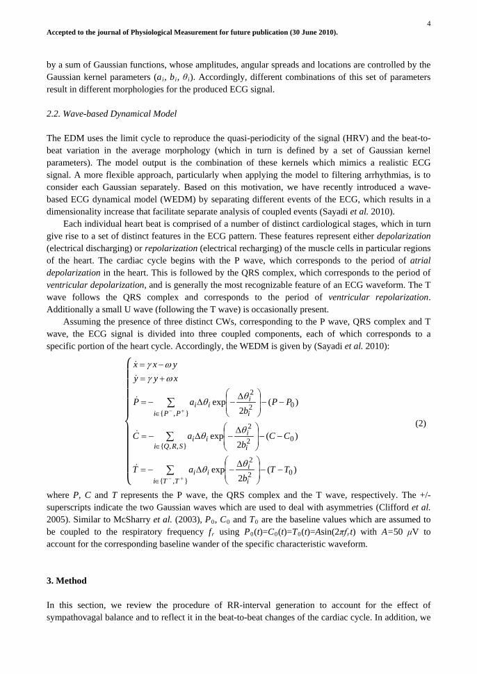
by a sum of Gaussian functions, whose amplitudes, angular spreads and locations are controlled by the Gaussian kernel parameters (ai, bi, θ i

). Accordingly, different combinations of this set of parameters result in different morphologies for the produced ECG signal.

2.2. Wave-based Dynamical Model The EDM uses the limit cycle to reproduce the quasi-periodicity of the signal (HRV) and the beat-to-beat variation in the average morphology (which in turn is defined by a set of Gaussian kernel parameters). The model output is the combination of these kernels which mimics a realistic ECG signal. A more flexible approach, particularly when applying the model to filtering arrhythmias, is to consider each Gaussian separately. Based on this motivation, we have recently introduced a wave-based ECG dynamical model (WEDM) by separating different events of the ECG, which results in a dimensionality increase that facilitate separate analysis of coupled events (Sayadi et al. 2010).

Each individual heart beat is comprised of a number of distinct cardiological stages, which in turn give rise to a set of distinct features in the ECG pattern. These features represent either depolarization (electrical discharging) or repolarization (electrical recharging) of the muscle cells in particular regions of the heart. The cardiac cycle begins with the P wave, which corresponds to the period of atrial depolarization in the heart. This is followed by the QRS complex, which corresponds to the period of ventricular depolarization, and is generally the most recognizable feature of an ECG waveform. The T wave follows the QRS complex and corresponds to the period of ventricular repolarization. Additionally a small U wave (following the T wave) is occasionally present.

Assuming the presence of three distinct CWs, corresponding to the P wave, QRS complex and T wave, the ECG signal is divided into three coupled components, each of which corresponds to a specific portion of the heart cycle. Accordingly, the WEDM is given by (Sayadi et al. 2010):

⎩⎪⎪⎪⎪⎨

⎪⎪⎪⎪⎧

)(2

exp

)(2

exp

)(2

exp

0},{

2

2

0},,{

2

2

0},{

2

2

TTb

aT

CCb

aC

PPb

aP

xyyyxx

TTi i

iii

SRQi i

iii

PPi i

iii

−−

∆−∆−=

−−

∆−∆−=

−−

∆−∆−=

+=−=

∑

∑

∑

+−

+−

∈

∈

∈

θθ

θθ

θθ

ωγωγ

�

(2)

where P, C and T represents the P wave, the QRS complex and the T wave, respectively. The +/- superscripts indicate the two Gaussian waves which are used to deal with asymmetries (Clifford et al. 2005). Similar to McSharry et al. (2003), P0, C0 and T0 are the baseline values which are assumed to be coupled to the respiratory frequency fr using P0(t)=C0(t)=T0(t)=Asin(2πfr

t) with A=50 μV to account for the corresponding baseline wander of the specific characteristic waveform.

3. Method In this section, we review the procedure of RR-interval generation to account for the effect of sympathovagal balance and to reflect it in the beat-to-beat changes of the cardiac cycle. In addition, we


incorporate optional parameters in the model to control the synthetic ECG parameters such as observational uncertainty and the sampling frequency. Afterwards, we show the new form of the dynamic equations (2) in polar coordinates, according to which a discrete state space representation is acquired to construct Bayesian framework for denoising applications. 3.1. Synthetic ECG generation As stated before, the wave-based dynamical model (2) generates the three CWs which are separate in z dynamics, but are coupled in timing as well as in nature. The model has 7 events, i.e. {P ˉ, P +, Q, R, S, T ˉ, T +

}, that act as push-pulls in the z direction as the corresponding trajectory passes around the unit limit cycle in the (x, y) plane. By contrasting the dynamical model (2) with the mechanisms underlying the cardiac cycle, it is obvious that the time required to complete one lap of the limit cycle is equal to a single beat duration and can be considered as the RR-interval of the synthetic ECG signal. On the other hand, the RR sequence timing can be assumed equal to the PP and TT sequences, since they all result from a physiological subsequence. Hence, variations in the length of the intervals can be incorporated by varying the same parameter, the angular velocity ω, to include the sequential coupling of the CW occurrence. To simulate the quasi-periodicity of the synthetic cardiac cycle, the time-dependent angular frequency of motion around the limit cycle is given by:

)(2)(

tRt πω =

(3)

where R(t) represents the time series generated by the RR-process, which introduces variations in the instantaneous heart rate time series using the generated beat-to-beat RR-intervals (the RR tachogram). Physiologically speaking, the heart rate may be increased by slow acting sympathetic activity or decreased by fast acting parasympathetic (vagal) activity. The balance between the effects of these two opposite acting branches of the autonomic nervous system is referred to as the sympathovagal balance and is believed to be reflected in the beat-to-beat changes of the cardiac cycle (Malik and Camm 1995). To incorporate the effect of the sympathetic and parasympathetic modulation of the RR-intervals, we have applied the same spectral estimation strategy as McSharry et al. (2003). In fact, the RR-process is supposed to generate RR-intervals which have a bimodal power spectrum consisting of the sum of two Gaussian distributions, whose parameters are motivated by the typical power spectrum of a real RR tachogram (Malik and Camm 1995). Having established the generation procedure for the RR-process, we are able to the use the synthetic model (2) for realistic CW generation. To solve the equations of motion (2) for generating synthetic CWs, they are integrated numerically using a fourth-order Runge–Kutta method (Press et al. 1992) with a fixed time step Δt=1/ fs where fs is the sampling frequency of the generated discrete ECG waveform. In order to simplify the dimensions and later relate the model parameters with real ECG recordings, the ai

terms in (2) will be replaced with:

},,,,,,{2+−+−∈= TTSRQPPi

ba

i

ii

ωα

(4)

where the α i are the peak amplitudes of the Gaussian functions used for modeling each of the ECG components (Sameni et al. 2007b). This definition may be verified from (2), by neglecting the baseline wander term (z − z0 z) and integrating the equation with respect to t. The ECG generation is now straight forward. Since the solution of (2) gives the time-series P(t), C(t) and T(t), the synthetic ECG is obtained by:

)()()()( tTtCtPtECG ++= (5)


3.2. Bayesian filtering A classical problem in estimation theory is the estimation of the hidden states of a system with an underlying dynamic model that are observable through a set of measurements. The well-known Kalman filter (KF) is one such method and under certain general constraints, it can be proved to be the optimal filter in the minimum mean square error sense (Kay 1993).

In the previous subsection, it was shown that realistic ECG signals can be produced by integrating a set of motion equations which modeled distinct CW of an ECG signal. However, since the equation set (2) is a state space representation, it can be used for a Bayesian paradigm construction. In the following, the proposed model (2) is used to model the temporal dynamics of ECG signals in a Bayesian framework for ECG denoising. Following the proposal of Sameni et al. (2005), we benefit the polar representation of the dynamical equations (2). With the proposed substitution (4), the new form of the dynamic equations in polar coordinates can be expressed as:

⎩⎪⎪⎪⎪⎨

⎪⎪⎪⎪⎧

)(2

exp

)(2

exp

)(2

exp

)1(

0},{

2

2

2

0},,{

2

2

2

0},{

2

2

2

TTbb

T

CCbb

C

PPbb

P

rrr

TTi i

i

i

ii

SRQi i

i

i

ii

PPi i

i

i

ii

−−

∆−

∆−=

−−

∆−

∆−=

−−

∆−

∆−=

=−=

∑

∑

∑

+−

+−

∈

∈

∈

θθωα

θθωα

θθωα

ωϕ

�

(6)

where r and φ are the radial and angular state variables in polar coordinates, respectively. Similar to polar version of McSharry’s model introduced by Sameni et al. (2007), this new set of equations has some benefits compared with the original equations (2). Firstly, the radial behavior of the generated trajectory converges to the limit cycle of r=1 for any initial value of r≥1. However, the second to fifth equations of (6) are independent of r, making the first equation redundant. Therefore, this first equation may be excluded as it does not affect the synthetic CWs (the P, C and T state variables). This leads to a simpler representation with straightforward interpretation. Secondly, the phase parameter φ is an explicit state-variable that indicates the angular location of different events, which is further used for the implementation of Bayesian ECG filters. In order to construct the discrete state space model used in Bayesian filters, we use a variant of (6) in its discrete form. The discrete state space representation in polar coordinates is given by:

⎩⎪⎪⎪⎪⎨

⎪⎪⎪⎪⎧

k

k

k

k

kk

k

k

k

k

kk

k

k

k

k

kk

TTTi i

i

i

iikk

CSRQi i

i

i

iikk

PPPi i

i

i

iikk

kk

bbTT

bbCC

bbPP

ηθθω

αδ

ηθθω

αδ

ηθθω

αδ

πωδϕϕ

+

∆−

∆−=

+

∆−

∆−=

+

∆−

∆−=

+=

∑

∑

∑

+−

+−

∈+

∈+

∈+

+

},{2

2

21

},,{2

2

21

},{2

2

21

1

2exp

2exp

2exp

)2mod()(

�

(7)


where δ is the sampling period, φ is the wrapped phase in polar coordinates and πθϕθ 2mod)(

kk iki −=∆ . Moreover, the inaccuracies of the dynamic model including the baseline

wander and the respiration modulation are replaced by perturbation terms ηP, ηC and ηT

Having considered four equations in (7) as the state space representation for the ECG signal, the process equations of a Bayesian framework are formed. Relating the ECG signal as an observation to the state variables in the left side of state space model (7) is now straightforward, since the CWs are summed up to form the record. In addition, a saw-tooth-shape signal that is expected to be zero at R-peaks, and being linearly assigned a phase between −π and π to the intermediate samples is also formed as the other observation. The observed noisy phase

, which are random additive noises.

kφ and noisy amplitude kz of the ECG are given by:

�k

k

uTCPz

u

kkkk

kk

2

1

+++=

+= ϕφ �

(8)

where k

u1 and k

u2 are the observation noises of the ECG in the phase and spatial domains,

respectively. The estimation of the states of the nonlinear model (7) that are observable through a set of measurements (8) is possible through an extended Kalman filter. Our proposed framework is built upon an EKF structure for its simplicity and improved numerical stability over other Bayesian filters (Gelb 1974). In order to use the KF formalism for this system, it is necessary to derive a linear approximation of (7) near a desired reference point, to obtain the following linear approximate model:

�

)ˆ()ˆ(),ˆ,ˆ(),,()ˆ()ˆ(),ˆ,ˆ(),,(1

kkkkkkkkkkk

kkkkkkkkkkkvvNxxMkvxgkvxgy

wwBxxAkwxfkwxfx−+−+≈=

−+−+≈=+ �

(9)

where f is the state evolution function and g represents the relationship between the state vector and the observations. The state variables vector, kx , the observation vector,

ky , the process noise vector, kw ,

and the observation noise vector, kv , are defined as follows:

][

},,,,,,{,],,,,,,[

][][

21 ′=

∈′=

′=

′=

+−+−

kk

kkkkkk

uuv

TTSRQPPibw

zyTCPx

k

TCPiiik

kkk

kkkkk

ηηηωθα

φϕ

(10)

where the prime indicates the transpose operator. The EKF algorithm is implemented using the time propagation and the measurement propagation equations to estimate the state variables (Kay 1993). The key idea for the implementation of the EKF is to linearize the nonlinear dynamical model in the vicinity of the previous estimated point, and to recursively calculate the state covariance matrices from the linearized equations, while the KF time propagation is performed via the original nonlinear equation (Haykin 2001).

The parameters of linearized model for time and measurement propagation in the EKF structure can be obtained using the equation set (7), (8) and the coefficients of the linear approximate model (9). To simplify the equations of the linearized model, we define the following terms for i ∈ {P ˉ, P +, Q, R, S, T ˉ, T +

}:


[ ] 3122134221234234

2

243

21

)1)(()1)(5.0(2

)2

exp(,

,,

×−−=ℵ

∆−−==

∆==

iiiiii

i

ii

ii

i

ii

i

ii

bb

bb

λλλλλ

θδλωλ

θλαλ

(11)

where dcbaabcd λλλλλ = . According to this terminology, the linearization of (7) and (8) with respect to the process components yields the following linear approximate coefficients:

=

∂∂

=

=

∂∂

=

ℵℵ

ℵℵℵ

ℵℵ

=∂

∂=

−

−

−

=∂

∂=

==

×∈×

∈××

∈×

×

=

×∈

∈

∈

=

∑

∑

∑

∑

∑

∑

+−+−

+−+−

+−

+−

1001),,ˆ(

,11100001),ˆ,(

1000

01000

00100000

),,ˆ(

100))(1(

010))(1(

001))(1(0001

),ˆ,(

ˆˆ

254},{

124115

},,{

1241616

},{

124115

121

ˆ

44},{

22134},,{

22134},{

22134

ˆ

kk

k

k

vvk

kxx

kk

TTiiTT

SRQiiSRQ

PPiiPP

wwk

k

TTiii

SRQiii

PPiii

xxk

k

vkvxg

Nx

kvxgM

wkwxf

B

xkwxf

A

λ

λ

λδ

λλ

λλ

λλ

(12)

To improve the filtering performance, it is also possible to use the information of future observations in the estimation procedure. This idea leads to the extended Kalman smoother (EKS). The EKS uses the future observations to give better estimates of the current state. The EKS algorithm basically consists of a forward EKF stage followed by a backward recursive smoothing stage. Due to this non-causal nature, the EKS is expected to have a better performance compared with the EKF. Depending on the smoothing strategy, smoothing algorithms are usually classified into fixed lag or fixed interval smoothers (Gelb 1974). In this paper, the fixed interval EKS is used, since the filtering procedure is carried out offline on the entirety of each ECG signal. For real-time applications of the proposed EKS methods, the fixed lag smoother is usually more appropriate.

The proposed nonlinear Bayesian framework estimates its variables using the state dynamical equations (7) and the noisy phase and noisy ECG observations. Having derived the state equations (7), the observation equations (8), and the linearized state equations of the ECG dynamic model (12), the implementation of the EKF and EKS is now possible. The filtering procedure provides the estimations corresponding to the CWs of the input ECG signal, which are summed up to obtain the denoised signal:

∑=

=++=4

2ˆˆˆˆˆ

iikkkk k

xTCPz

(13)

The denoising block diagram is shown in figure 1, in which the phase calculation block is simply an R-peak location detector, followed by linear assigning of a phase value between -π and π to the intermediate samples (Sameni et al. 2007b). In fact the ECG signal along with the phase signal forms the observation vector for the EKF structure. The initialization process is then run on this vector, to


Figure 1. General block diagram of the proposed algorithm for ECG denoising.

find the initial value for the state vector, the covariance matrices of the process noise and the measurement noise. Finally, the estimations of the state variables are obtained using the KF formulation.

4. Simulation Results The proposed algorithms were implemented in MATLAB®. The same RR-process generator as McSharry et al. (2003) was used for generating synthesized ECG signals with user-defined parameters (McSharry and Clifford 2003). Standard ECG databases from Physiobank, the Physionet signal archives (Golberger et al., 2000) were used to study the performance of the proposed denoising method. The initialization procedure described by Sameni et al. (2007) and Sayadi and Shamsollahi (2008) is employed for KF initialization. Qualitative and quantitative results are presented next. 4.1. Synthetic ECG generation

The described model gives the opportunity to have control on various signal parameters, such as the CW amplitude, spread and angular location, sampling frequency, mean and standard deviation of heart rate, noise amplitude, respiratory modulation frequency, and the ratio of the power contained in the low-frequency and high-frequency components of the tachogram spectrum. Figure 2 shows typical CW trajectories generated by the dynamical model (7) in the 3D space given by (x, y, z), with the limit cycle of unit radius included. Also, the distinct synthesized CWs are shown as a function of time, each of which is coupled with other CWs on a sequential time occurrence. The synthetic realistic ECG can be obtained by simply adding these three components, as shown in figure 2(c). The RR-tachogram and the corresponding bimodal power spectrum are shown in figure 2(d), 2(e) respectively, generated with mean heart rate 60 beats-per-minute and standard deviation 5 beats-per-minute.

As it can be seen, the synthetic ECG mimics the morphology of a real ECG signal. In addition, the RR-interval tachogram has a realistic spectral content. In other words, the dominant peak in the high-frequency band of the spectrum (≈ 0.25 Hz) is as the result of parasympathetic oscillations called respiratory sinus arrhythmia (RSA), while the second peak which is often found in the low-frequency band (≈ 0.1 Hz) is due to baroreflex regulation which creates the so-called Mayer waves in the blood pressure signal (De Boer et al. 1987).

ϕ

C

P

Denoised ECG

T

Extended

Kalman

Filter /

Smoother

Phase Calculation

ECG


(a) (b)

(c)

(d) (e)

(f) (g)

(h)

Figure 2. Wave-based synthetic ECG generation. (a) CW trajectories in the Cartesian coordinates, (b) Synthetic CWs as functions of time, (c) realistic synthesized ECG, (d) RR-interval tachogram of the generated ECG using the proposed RR-process, (e) Bimodal power spectrum of the generated RR-intervals, including the Mayer and RSA waves, (f) RR-interval tachogram of a typical real ECG signal, (g) Power spectrum of the real RR-intervals shown in (f) obtained from the typical ECG record, (h) realistic synthesized ECG using the real RR-interval tachogram.

In order to have a more similar spectral contents to real HRV spectra, it is possible to use real heart

rate variability signals acquired from real ECG signals, instead of generating artificial RR-tachograms using the proposed RR-process (section 3.1). Although this approach results in more realistic synthetic signals, the model is perhaps less useful for evaluating signal processing methods when used in this way. This is because standard pre-defined parameters such as those used in the RR-process generation cannot be accurately specified. Figure 2(h) shows a typical generated ECG signal using this approach, in which the RR-tachogram (figure 2(f)) is obtained to mimic a real HRV spectrum (figure 2(g)).

-2

-1

0

1

-1.5-1-0.500.51-0.01

0.01

0.03

XY

Z

PQRSTlimit cycle

11 12 13 14 15 16-0.03

-0.01

0.01

0.03

Time (sec)

Am

plitu

de (m

V)

P QRS T

11 12 13 14 15 16 17 18 19-0.02

-0.01

0

0.01

0.02

0.03

Time (sec)

Ampli

tude (

mV)

0 50 100 150 200 250 300 350 400 450 5000.95

1

1.05

Beat number

RR

inte

rval

(sec

)

0 0.05 0.1 0.15 0.2 0.25 0.3 0.35 0.4 0.45 0.50

0.5

1

1.5

2

Normalized frequency

Pow

er (s

ec2 /H

z)

0 50 100 150 200 250 300 350 400 450 500

0.8

0.9

1

1.1

1.2

1.3

Beat Number

RR

inte

rval

(sec

)

0 0.05 0.1 0.15 0.2 0.25 0.3 0.35 0.4 0.45 0.50

0.5

1

1.5

2

2.5

3

Normalized Frequency

Pow

er(s

ec2 /H

z)

0 1 2 3 4 5 6 7 8 9 10-0.2

0

0.2

0.4

0.6

Time (sec)

Ampli

tude (

mV)


(a) (b)

(c) (d) 2

(e)

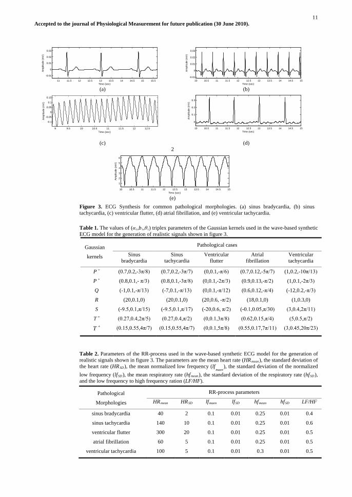
Figure 3. ECG Synthesis for common pathological morphologies. (a) sinus bradycardia, (b) sinus tachycardia, (c) ventricular flutter, (d) atrial fibrillation, and (e) ventricular tachycardia.

Table 1. The values of (α i,bi,θ i

) triplex parameters of the Gaussian kernels used in the wave-based synthetic ECG model for the generation of realistic signals shown in figure 3.

Gaussian

kernels

Pathological cases

Sinus bradycardia

Sinus tachycardia

Ventricular flutter

Atrial fibrillation

Ventricular tachycardia

P ˉ

(0.7,0.2,-3π/8)

(0.7,0.2,-3π/7)

(0,0.1,-π/6)

(0.7,0.12,-5π/7)

(1,0.2,-10π/13)

P (0.8,0.1,- π/3) + (0.8,0.1,-3π/8) (0,0.1,-2π/3) (0.9,0.13,-π/2) (1,0.1,-2π/3)

Q (-1,0.1,-π/13) (-7,0.1,-π/13) (0,0.1,-π/12) (0.6,0.12,-π/4) (-12,0.2,-π/3)

R (20,0.1,0) (20,0.1,0) (20,0.6, -π/2) (18,0.1,0) (1,0.3,0)

S (-9.5,0.1,π/15) (-9.5,0.1,π/17) (-20,0.6, π/2) (-0.1,0.05,π/30) (3,0.4,2π/11)

T ˉ (0.27,0.4,2π/5) (0.27,0.4,π/2) (0,0.1,3π/8) (0.62,0.15,π/4) (5,0.5,π/2)

T (0.15,0.55,4π/7) + (0.15,0.55,4π/7) (0,0.1,5π/8) (0.55,0.17,7π/11) (3,0.45,20π/23)

Table 2. Parameters of the RR-process used in the wave-based synthetic ECG model for the generation of realistic signals shown in figure 3. The parameters are the mean heart rate (HRmean), the standard deviation of the heart rate (HRSD), the mean normalized low frequency (lf

maen), the standard deviation of the normalized

low frequency (lfSD), the mean respiratory rate (hfmean), the standard deviation of the respiratory rate (hfSD

), and the low frequency to high frequency ration (LF/HF).

Pathological

Morphologies

RR-process parameters

HR HRmean lfSD lfmaen hfSD hfmean LF/HF SD

sinus bradycardia

40

2

0.1

0.01

0.25

0.01

0.4

sinus tachycardia 140 10 0.1 0.01 0.25 0.01 0.6

ventricular flutter 300 20 0.1 0.01 0.25 0.01 0.5

atrial fibrillation 60 5 0.1 0.01 0.25 0.01 0.5

ventricular tachycardia 100 5 0.1 0.01 0.3 0.01 0.5

11 11.5 12 12.5 13 13.5 14 14.5 15 15.5

-0.01

0

0.01

0.02

0.03

Am

plitu

de (m

V)

Time (sec)10 10.5 11 11.5 12 12.5 13 13.5 14 14.5 15

-0.01

0

0.01

0.02

0.03

Am

plitu

de (m

V)

Time (sec)

9 9.5 10 10.5 11 11.5 12 12.5

-0.1

-0.05

0

0.05

0.1

0.15

Time (sec)

Am

plitu

de (m

V)

10 10.5 11 11.5 12 12.5 13 13.5 14 14.5 15

0

0.1

0.2

0.3

Time (sec)

Am

plitu

de (m

V)

10 10.5 11 11.5 12 12.5 13 13.5 14 14.5 15

1

2

3

4

5

6

Time (sec)

Am

plitu

de (m

V)


(a)

(b) (c)

Figure 4. Input noisy observations and the output denoised state variables of EKF4 for a typical ECG signal. (a) Noisy input phase (dashed) and ECG (solid) observations, (b) CW estimations, (c) Denoised phase signal (dashed) and the ECG signal (solid).

Since the model has several parameters, it is possible to control the morphological features of the

synthetic ECG. Accordingly, it is possible to introduce abnormal morphological changes with time using a parameter to control the position and the form of the events. This extension has been also tested to incorporate several pathological conditions. Figure 3 shows the results of generating synthetic normal and abnormal ECGs including two normal states (sinus bradycardia and sinus tachycardia) and three abnormalities (atrial fibrillation, ventricular flutter and ventricular tachycardia). The depictions are the model outputs for different set of input parameters. Visual analysis of different sections of typical ECGs - both normal and abnormal subjects - was used to suggest suitable times, amplitude and spread values for the events. The corresponding values of Gaussian kernel parameters are shown in table I. Table II lists the parameters of the RR-process used in the simulation, including the mean and the standard deviation of heart rate, normalized low frequency which corresponds to the Mayer waves, respiratory rate and LF/HF ratio. 4.2. Bayesian filtering According to (13), the estimations of the second to fourth state variables obtained by the proposed EKF model with 4 state variables (EKF4) was summed up to form the denoised ECG signal. The same story holds for the EKS model with 4 state variables (EKS4). The MIT-BIH Normal Sinus Rhythm Database (Goldberger et al. 2000, MIT-BIH Normal Sinus Rhythm Database 1991) and The MIT-BIH Noise Stress Test Database (Goldberger et al. 2000, MIT-BIH Noise Stress Test Database) were used to study the performance of the proposed denoising method. Figure 4 shows typical EKF4 estimations, i.e. the CW estimates, which are summed up to form the denoised ECG.

The effect of different types of noises including white and real noises on the performance of the proposed method is investigated in figure 5. Comparing these results visually, it can be seen that the proposed method have admirably tracked the original signal in a rather low input signal to noise ratio (SNR) scenario. Moreover, The EKS demonstrates a smoother result, compared to that of EKF. In particular, it can be seen that the denoised signal follows the clean ECG morphology when artificial white noise is added (Figure 5(a)). Likewise, for the real EMG noises, the denoised signal is free from any EMG artifacts (Figure 5(b)). Motion artifact is generally considered the most troublesome, since it

1 1.5 2 2.5 3 3.5 4 4.5 5 5.5-4

-2

0

2

4

Time (sec)

Ampl

itude

(rad

/sec

-mV)

φ z

1 1.5 2 2.5 3 3.5 4 4.5 5 5.5-2

-1

0

1

2

3

Time (sec)

Am

plitu

de (m

V)

P C T

1 1.5 2 2.5 3 3.5 4 4.5 5 5.5-4

-2

0

2

4

Time (sec)

Ampl

itude

(ra

d/se

c-m

V)

φ z


(a)

(b)

(c)

Figure 5. Typical filtering results of the proposed wave-based approach for different types of input noises using EKF4 and EKS4. The MIT-BIH Normal Sinus Rhythm Database (Goldberger et al. 2000, MIT-BIH Normal Sinus Rhythm Database 1991) is used for evaluation. (a) Record 118e24 with an additive white Gaussian noise of –2 dB. (b) Record 118e18 with calibrated amount of real EMG noise (input SNR of 4 dB for the noisy portion). (c) Record 118e06 with real motion artifacts (input SNR of 6 dB).

can mimic the appearance of ectopic beats, it causes undesired notches on the ST segment and cannot be removed easily by simple band pass filters, unlike other types. Figure 5(c) indicates that EKF4 is also able to remove motion artifact, while preserving diagnostic morphological information of the signal. Note that because there are underlying dynamics for the ECG signal which constrain the filtering, motion artifact cannot force the denoised signal follow distorted waveforms. To clarify this, see Figure 5(c), where the denoised signal shows a different pattern to that of the noisy signal. Specifically, the T-wave end points, the PQ intervals and the ST segments in the denoised signal do not follow the corresponding distorted portions of the noisy signal.

To appreciate the merits of the proposed methods over the previously Bayesian model with 2 state variables, i.e. EKF2 and EKS2 (Sameni et al. 2007b), we have depicted the results of extended Kalman smoothing with EKS2 and EKS4 in Figure 6. The mean ECG, the standard deviation, and the least squares fit are also provided. One can easily find the ST elevation distortions and the baseline perturbation distortions of EKS2. In addition, when the initialization is not reliable or it does not account for out-kernel waves such as U wave, EKS4 outperforms EKS2 (see the U wave distortions in Figure 6(b) and the T wave distortions in Figure 6(d) for EKS2). For evaluating the performance of the proposed method, we have used the SNR improvement measure given by:

−−= ∑∑

id

in ixixixixdBimp 22 )()(/)()(log10][

(14)

where x denotes the clean ECG, xd is the denoised signal and xn

In order to investigate the performance of our algorithm and to compare it to different benchmark methods, we have implemented all Kalman-based ECG filtering schemes including the proposed EKF4

represents the noisy ECG.

14 14.5 15 15.5 16 16.5 17 17.5

-3

-2

-1

0

1

2

3

4

Time (sec)

Ampl

itude

(mV)

Noisy EKF4 EKS4

10 10.5 11 11.5 12 12.5 13 13.5 14 14.5 15-2

-1

0

1

2

3

4

Time (sec)

Ampl

itude

(mV)

Noisy EKF4 EKS4

0 0.5 1 1.5 2 2.5 3 3.5

-1

0

1

2

3

4

5

6

Time (sec)

Ampl

itude

(mV)

Noisy EKF4 EKS4


(a) (c)

(b) (d)

Figure 6. Qualitative comparison of filtering performances for EKS2 and EKS4 using a normal (record 106) and an abnormal (record 104) ECG from the MIT-BIH Arrhythmia Database (Goldberger et al. 2000, MIT-BIH Arrhythmia Database). (a) Average and standard deviation-bar of 20 ECG cycles of the normal ECG. The vertical lines are initial seeds for LSE fit, (b) Filtering results for the input normal ECG of 5 dB (top), EKS2 output with 8.94 dB improvement (middle), and EKS4 output with 10.26 dB improvement (bottom), (c) Average and standard deviation-bar of 20 ECG cycles of the abnormal ECG, (d) Filtering results for the input abnormal ECG of 3.8 dB (top), EKS2 output with 7.03 dB improvement (middle), and EKS4 output with 9.89 dB improvement (bottom). The baseline perturbation distortions and the peaks distortions for EKS2 are clearly seen.

and EKS4 methods, the EKF2 and EKS2 algorithms (Sameni et al. 2007b), and EKF17 which is a parameter-based Bayesian framework with auto- regressive dynamics (Sayadi and Shamsollahi 2008). Also, the conventional wavelet transform (WT) has been tested on the database. The reported results are based on the Coiflets3 mother wavelet with 6 levels of decomposition using the Stein’s Unbiased Risk Estimate (SURE) shrinkage rule, together with a single level rescaling and a soft thresholding strategy, as was tested by Sameni et al. (2007). For performance evaluation, Sameni et al. (2007) used 190 ECG segments from the the first 13 records of the MIT-BIH Normal Sinus Rhythm Database (Goldberger et al. 2000, MIT-BIH Normal Sinus Rhythm Database 1991). We have used the same records, however to ensure the consistency of the results, the full-length of the records were used for simulation. The whole procedure was repeated 50 times over the first 60 minutes of the selected records; each time using the same initial parameters but with a different set of random white Gaussian noise at the input. The SNRs were generally calculated over the second half of the filtered segments, to ensure that the transient effects of the filters would not influence the SNR calculations. For a quantitative comparison, the mean and standard deviation (SD) of the SNR improvements versus different input SNRs are depicted in Figure 7.

It can be seen that the EKS4 demonstrates the best average performance, and the EKF4 performs marginally better than the EKF2, is much similar to EKF17, but still underperforms the EKS2 approach. Furthermore, the superiority of EKS4 is obvious, especially in lower input SNRs, where the clean ECG is lost in noise.

Mathematically, white noise is defined to have a flat spectral density function over all frequencies. However, real noise sources have non-flat spectral densities that decrease in power at higher

0 0.5 1 1.5 2 2.5 3 3.5 4-1400

-1200

-1000

-800

-600

-400

-200

0

200

400

600

Time (sec)

Am

plitu

de(m

V)

ECG

EKS4

EKS2

0 0.5 1 1.5 2 2.5 3 3.5 4-800

-700

-600

-500

-400

-300

-200

-100

0

100

200

Time (sec)A

mpl

itude

(mV

)

EKS4

EKS2

ECG


(a) (b)

Figure 7. The mean (left) and variance (right) of the filter output SNR improvements for white noise versus different input SNRs averaged over 50 repetitions for different filtering methods, including WT, EKF2, EKS2, EKF17, EKF4 and EKS4.

frequencies, making the spectrum colored and the noise samples correlated in time. To have a better insight into the performance of the proposed Bayesian filter, artificial colored Gaussian noise with different variances were generated. For the current study, we have modeled the noise color by a single parameter representing the slope of a spectral density function that decreases monotonically with frequency:

cffS 1)( ∝

(15)

where f is the frequency and c is the slope; a measure of noise color. White noise (c=0), pink or flicker noise (c=1), and brown noise or the random walk process (c=2), are three of the most commonly referenced noises (Kay 1981).

Besides colored noises, calibrated amount of real noises were added to the ECG segments, and the noisy signals were presented to the benchmark and the proposed filters. The results of the noise color and real noise study are depicted in figure 8 for the mean SNR improvement as a function of the input SNR for all filtering methods. As can be seen, the filter performance increases as the input SNR ranges from 24 dB to -6 dB, while the slope of increase is larger for the proposed wave-based algorithms, i.e. EKF4 and EKS4. As with the previous results, it is seen that the EKS4 outperforms the results with all other techniques. In the presented approach, due to the phase wrapping of the RR interval to 2π, normal inter-beat variations of the RR-interval or consistent RR-interval abnormalities such as bradycardia or tachycardia do not considerably affect the filter performance. However, for morphological abnormalities that only appear in some of the ECG cycles, such as the Premature Ventricular Contraction (PVC), the phase error of the model can lead to large errors in the Gaussian functions’ locations. In particular, for low input SNRs, where neither the model nor the measurements are reliable for the filter, the filtering performance is not expected to be satisfactory. However, the benefit of the Gaussian mixture representation is that the effect of each Gaussian term vanishes very quickly (in less than the ECG period), meaning that the errors are not propagated to the following ECG cycles. In addition, the wave-based structure enables the model to have less error propagations due to the separation of Gaussian kernels. Figure 9 shows typical filtering results of an ECG signal with a spontaneous PVC rhythm. It can be seen that EKF4 and specially EKS4 provide a more accurate representation of the signal and

20151050-50

2

4

6

8

10

12

Input SNR (dB)

SN

R Im

prov

emen

t (dB

)

WTEKF2EKS2EKF17EKF4EKS4

20151050-5

1.5

2

2.5

3

3.5

4

4.5

Input SNR (dB)

SN

R Im

prov

emen

t Var

ianc

e (d

B)

WTEKF2EKS2EKF17EKF4EKS4


(a) (b)

(c)

Figure 8. The mean SNR improvements versus different input SNRs averaged over 50 repetitions for different filtering methods, including WT, EKF2, EKS2, EKF17, EKF4 and EKS4 for (a) pink noise, (b) brown noise, and (c) real EMG noise.

Figure 9. Typical filtering results of an ECG signal with a spontaneous PVC rhythm using EKF2, EKS2, EKF4 and EKS4. Record 119 from the MIT-BIH Arrhythmia Database (Goldberger et al. 2000, MIT-BIH Arrhythmia Database) is used for simulation (dotted line). The denoised signals are shown with solid lines.

track the rhythm change with less error in kernel assignments than EKF2 and EKS2. It should be mentioned that by monitoring the state estimates’ covariance matrices and the variations of the

WTEKF2

EKF4EKF17

EKF4EKS4

2418

126

0-6-5

0

5

10

15

20

25

MethodsInput SNR (dB)

Mea

n S

NR

Impr

ovem

ent (

dB)

WTEKF2

EKF4EKF17

EKF4EKS4

2418

126

0-6-5

0

5

10

15


Mea

n S

NR

Impr

ovem

ent (

dB)

WTEKF2

EKS2EKF17

EKF4EKS4

2418

126

0-6-5

0

5

10

15

20


Mea

n S

NR

Impr

ovem

ent (

dB)

4.5 5 5.5 6 6.5 7 7.5 8 8.5Time (sec)

Ampl

itude

EKF2

EKS2

EKF4

EKS4


innovation signals, it is possible to detect such unexpected abnormalities and hence, change the Kalman parameters to rely more on the observed cycle that the underlying dynamics (Sayadi et al. 2010).

It is also worth noting that the model presented in this article can also be used for fiducial point detection, since the θ i in equation (2), which are traced from beat-to-beat determine the locations or each CW. Clifford and Villarroel (2006) showed how the onset and offset of the CW's can be found, even for composite Gaussians, using a set number of standard deviations from the central time location of the θ i

The figures demonstrate that the deviations behave like a normal distribution. Moreover, for the PR interval which is defined as the difference between peak locations of P wave and QRS complex, the error is not considerable (mostly below 8 ms). However, the asymmetric properties of T wave and theway the corresponding two Gaussian kernels are related to the peak location results in more deviations, but still well in the acceptable range (below 36 ms), even for common difficulties such as standard ECG noise, P- and T-wave splitting, low amplitude T-waves and R-on-T or T-U fusion. Note that the TP interval is a pretty good proxy for the QT interval and that the 95% region is +/-5ms, which is better than inter-observer differences in annotating QT intervals (Moody et al. 2006) and conforms to the EACAR

. However, since ECG segmentation is not within the scope of the current study, we just show simple examples of two interval extractions based on peak detection results. Thus, to assess the accuracy of the EKF investigate the segmentation results of the proposed model-based algorithm with real clinical parameters, histograms of deviations between the markings of the automatic algorithm compared to the ‘gold standard’ of manually measured PR intervals and TP intervals for the 13 patients are presented in figure 10.

1

Another important issue is the limited range of deviations and their relation to the sampling frequency of the records. Figure 10 implies that the deviation lies in the interval of [−8, 8] ms for PR interval and [−36, 25] ms for TP interval extraction. Since the sampling frequency is 128 Hz, the former corresponds to 1 or 2 sample difference, and the latter corresponds to maximum 5 samples deviation from the manually located points. However, it was shown that for higher sampling frequencies (such as 360 Hz), the error is expected to be fewer than the above results (Sayadi and Shamsollahi 2008b).

guidelines. Based on this, it can definitely be said that the proposed automated method possess acceptable accuracy for clinical evaluations. Furthermore, combining the tracking properties of the EKF structure with the model-based idea, accuracy close to the experts’ measurements can be obtained.

(a) (b)

Figure 10. Histograms of deviations between the markings of the proposed automatic algorithm compared to the ‘gold standard’ of manually measured indices including (a) PR interval (b) TP interval.

1 The Expert Working Group (Efficacy) of the International Conference on Harmonisation of Technical Requirements for Registration of Pharmaceuticals for Human Use (ICH) (Branch 2005).

-8 -6 -4 -2 0 2 4 6 80

50

100

150

200

250

300

350

Deviation (ms)

Num

ber

95%

99%

-36 -30 -24 -18 -12 -6 0 6 12 18 240

50

100

150

200

250

300

350

Deviation (ms)

Num

ber

95%

99%


5. Discussion and Conclusions A wave-based dynamical set of motion equations was described and validated for synthetic ECG and CW generation, according to which a Bayesian framework was proposed for real ECG filtering. The model is based on a four dimensional state space that incorporates the characteristic waves of the ECG into a dynamical model. By separating the Gaussian functions, and using 2 kernels for asymmetric P and T waves, a state space model was constructed. The proposed set of equations aims at integrating into the ECG model a mechanism that estimates an ECG signal as a combination of finite characteristic waveforms, each of which represents a particular physiological state of the heart.

The model is capable of replicating many of the important features of the human ECG, including the morphological features and the spectral characteristics. In fact, many of the morphological changes observed in the real ECGs manifest as a consequence of the geometrical structure of the model. The model parameters control the specifications of the synthesized ECG, and in particular the average morphology can be controlled by specifying the positions of the P, Q, R, S, and T events and the magnitude of their effect on the ECG. Having access to a realistic ECG provides a benchmark for testing biomedical signal processing techniques. Accordingly, it is important to know how they perform for different noise levels and sampling frequencies. In addition, separation of different characteristic waveforms enables us to have control on separate physiological states, which are coupled together via the angular frequency parameter.

On the other hand, the state space model provides a means of KF-based tracking the behavior of the CWs, throughout the filtering procedure. From a filtering point of view, KFs can be thought of as adaptive filters that continuously move the location of the poles and zeros of their transfer functions, according to the signal or noise content of the input observations and the prior model of the signal dynamics. The filter structure is based upon a unique dynamical model, which is adapted to the observations according to the propagation equations. Moreover, this feature allows the filter to adapt with different spectral shapes and temporal nonstationarities, since the variance of the observation noise represents the degree of reliability of a single observation, as well as the degree of adaptively tracking the input noisy measurement. Based on this concept, we used the state variables estimations to obtain a denoised version of the input signal. The underlying dynamics (7) together with the KF structural covariance matrices guarantee the preservation of the signal morphology throughout the filtering procedure. The designed filter was applied to standard ECG databases. Compared to benchmark denoising schemes, the proposed EKF4 and EKS4 provides a larger SNR improvement, especially in lower input SNRs, where the original signal is lost in noise.

The use of adaptive Gaussian filters had been previously reported (Hodson et al. 1981, Talmon et al. 1986), where the frequency response of a convolutive Gaussian filter was adapted to the estimates of the local properties of the signal in order to minimize the distortion of the undisturbed signal by the filter. The major drawback of these methods is the template waveform construction which results in a complex method with increased processing time (Talmon et al. 1986). However, the EKF-based technique does not depend on a template, and instead uses a dynamic state space representation for adaptive signal tracking. Moreover, unlike the digital filters that depends on the phase alignment and bandwidth control (De Pinto 1991), the Kalman filters does not need any spectral adjustments.

Another point of interest is the low variance of SNR improvements for EKF4 and EKS4, which ensures the consistency of results as compared to other methods. Furthermore, the new modifications in the EKF structure results in fewer peak distortions and baseline perturbations tracking. This is true not only for white noise cases, but also for colored and real noises. In particular, the filter is more consistent while encountering spontaneous arrhythmias than the previously published methods. Hence,


the proposed method can serve as a basis for the design of a robust ECG filter, with applications for low SNR ECGs.

As an advantage, the model in its current form can be effectively used for ECG segmentation and fiducial points extraction. In fact, since the wave-based model provides separate estimation of the characteristic waves, the point extraction procedure can be much easier than point localization on the ECG signal. Furthermore, similar analytic expressions to Sayadi and Shamsollahi (2009) can be used for feature extraction from the characteristic waves of the ECG recordings.

In summary, the main contributions of this work are: 1) the introduction of a wave-based state space formulation for generating different types of pathologic ECG waveforms, 2) the derivation of a linearized model and the establishment of linear observation relations, 3) the proposal of a Kalman-based filtering scheme that could provide robust estimations of the input noisy measurements, and 4) the determination of ECG fiducial points based on the wave-based structure. Future works include incorporating non-Gaussian dynamics into the model to have a physiological correspondence for the asymmetric CWs. In addition, through modification of the RR-process, and especially by assigning nonlinear phases to the intermediate samples between R peaks, the time consequence of the CWs would be controlled, to produce pathological conditions such as QT prolongation and escape beats. Moreover, it is possible to use the methodology proposed by Clifford et al. (2010) and employ a first-order Markov chain to incorporate the transitions from normal to arrhythmia. Probability transitions can be learned from real data or modeled by coupling to heart rate and sympathovagal balance.

References Barros A K, Mansour A and Ohnishi N 1998 Removing artifacts from electrocardiographic signals using independent components analysis Neurocomputing 22 173–86 Branch S 2005 Guidelines from the International Conference on Harmonisation (ICH) J. Pharmaceutical and Biomedical Analysis 38 798-805 Clifford G D, Nemati S and Sameni R 2008 An Artificial Multi-Channel Model for Generating Abnormal Electrocardiographic Rhythms Proc. Comput. Cardiol. 14-17 Clifford G D, Shoeb A, McSharry P E and Janz B A 2005 Model-based filtering, compression and classification of the ECG Int. J. Bioelectromagn. 7 158–61 Clifford G D and Villarroel 2006 Model-Based Determination of QT Intervals Proc. Comput. Cardiol. 33 357–60 Clifford G D, Nemati S and Sameni R 2010 An artificial vector model for generating abnormal electrocardiographic rhythms Physiol. Meas. 31 (4) (In Press) Clifford G D and Tarassenko L 2001 One-pass training of optimal architecture auto-associative neural network for detecting ectopic beats Electron. Lett. 37 1126–27 Daqrouq K 2005 ECG baseline wander reduction using discrete wavelet transform Asian J. Inf. Technol. 4 989–95 De Boer R W, Karemaker J M and Strackee J 1987 Hemodynamic fluctuations and baroreflex sensitivity in humans: a beat-to-beat model Amer. J. Physiol. 253 680–89 De Pinto V 1991 Filters for the reduction of baseline wander and muscle artifact in the ECG J. Electrocardiol. 25 (Suppl.) 40–48 Donoho D L 1995 De-noising by soft-thresholding IEEE Trans. Inf. Theory 41 613–27 Gelb A 1974 Applied Optimal Estimation (Cambridge, MA: MIT Press) Goldberger A L, Amaral L A N, Glass L, Hausdorff J M, Ivanov P C, Mark R G, Mietus J E, Moody G B, Peng C K and Stanley H E 2000 PhysioBank, PhysioToolkit, and PhysioNet: components of a new research resource for complex physiologic signals Circulation 101 e215–20 (Circulation electronic pages http://circ.ahajournals.org/cgi/content/full/101/23/e215) He T, Clifford G D and Tarassenko L 2006 Application of independent component analysis in removing artefacts from the electrocardiogram Neural Comput. Appl. 15 105–16 Hodson E K, Thayer D R and Franklin C 1981 Adaptive Gaussian filtering and local frequency estimates using local curvature analysis IEEE Trans. Acoust. Speech Sig. Proc. 29 854–59 Kay S M 1981 Efficient generation of colored noise Proc. IEEE 69 480–81 Kay S M 1993 Fundamentals of Statistical Signal Processing: Estimation Theory (Englewood Cliffs, NJ: Prentice-Hall) Kestler H A, Haschka M, Kratz W et al.. 1998 De-noising of high-resolution ECG signals by combining the discrete wavelet transform with the Wiener filter Proc. Comput. Cardiol., (Cleveland, OH) 25 233–36 Malik M and Camm A J 1995 Heart Rate Variability (Armonk, NY: Futura) McSharry P E and Clifford G D 2003 ECGSYN - A realistic ECG waveform generator (http://www.physionet.org/physiotools/ ecgsyn/) McSharry P E, Clifford G D, Tarassenko L and Smith L A 2003 A dynamic model for generating synthetic electrocardiogram signals IEEE Trans. Biomed. Eng. 50 289–94 MIT-BIH Noise Stress Test Database (http://www.physionet.org/physiobank/database/nstdb/) MIT-BIH Normal Sinus Rhythm Database 1991 (http://www.physionet.org/physiobank/database/nsrdb/) Moody G B, Koch H and Steinhoff U 2006 The Physionet/Computers in Cardiology Challenge 2006: QT Interval Measurement Proc. Comput. Cardiol. 33 313-16

http://www.physionet.org/�


Moody G B and Mark R G 1989 QRS morphology representation and noise estimation using the Karhunen-Lo‘eve transform Proc. Comput. Cardiol. (Jerusalem, Israel) 16 269–72 PhysioBank, physiologic signal archives for biomedical research (http://www.physionet.org/physiobank/) Popescu M, Cristea P and Bezerianos A 1998 High resolution ECG filtering using adaptive Bayesian wavelet shrinkage Proc. Comput. Cardiol., 25 401–4 Press W H, Flannery B P, Teukolsky S A and Vetterling W T 1992 Numerical Recipes in C (2nd

Sameni R, Shamsollahi M B and Jutten C 2006 Multi-Channel Electrocardiogram Denoising Using a Bayesian Filtering Framework Proc. Comput. Cardiol. 17-20

ed. Cambridge, U.K.: Cambridge Univ Press)

Sameni R, Shamsollahi M B and Jutten C 2008 Model-based Bayesian filtering of cardiac contaminants from biomedical recordings Physiol. Meas. 29 595–613 Sameni R, Shamsollahi M B, Jutten C and Babaie-zadeh M 2005 Filtering Noisy ECG Signals Using the Extended Kalman Filter Based on a Modified Dynamic ECG Model Proc. Comput. Cardiol. 32 1017-20 Sameni R, Clifford G D, Jutten C and Shamsollahi M B 2007a Multichannel ECG and Noise Modeling: Application to Maternal and Fetal ECG Signals EURASIP Journal on Advances in Signal Processing Article ID 43407 doi:10.1155/2007/43407 Sameni R, Shamsollahi M B, Jutten C and Clifford G D 2007b A nonlinear Bayesian filtering framework for ECG denoising IEEE Trans. Biomed. Eng. 54 2172–85 Sayadi O, Sameni R and Shamsollahi M B 2007 ECG denoising using parameters of ECG dynamical model as the states of an extended Kalman filter Proc. EMBC’07 (Lyon, France) pp 2548–51 Sayadi O and Shamsollahi M B 2007 Multiadaptive bionic wavelet transform: Application to ECG denoising and baseline wandering reduction EURASIP J. Adv. Signal Process. 07 1–11 Sayadi O and Shamsollahi M B 2008a ECG denoising and compression using a modified extended Kalman filter structure IEEE Trans. Biomed. Eng. 55 2240–8 Sayadi O and Shamsollahi MB 2008b Model-based ECG fiducial points extraction using amodified extended Kalman filter structure Invited paper ISABEL ’08 (Aalborg, Denmark) pp 1–5 Sayadi O and Shamsollahi M B 2009 A model-based Bayesian framework for ECG beat segmentation Physiol. Meas. 30 335– 52 Sayadi O, Shamsollahi M B and Clifford G D 2010 Robust Detection of Premature Ventricular Contractions Using a Wave-Based Bayesian Framework IEEE Trans. Biomed. Eng. 57 353-62 Talmon J L, Kors J A and Van Bemmel J H 1986 Adaptive Gaussian filtering in routine ECG/VCG analysis IEEE Trans. Acoust. Speech Sig. Proc. 34 527–34 Thakor N V and Zhu Y S 1991 Applications of adaptive filtering to ECG analysis: Noise cancellation and arrhythmia detection IEEE Trans. Biomed. Eng. 38 785–94

Synthetic ECG Generation and Bayesian Filtering Using …lcp.mit.edu/pdf/SayadiPM10.pdf · 1...

Documents

Transcript of Synthetic ECG Generation and Bayesian Filtering Using …lcp.mit.edu/pdf/SayadiPM10.pdf · 1...