Synthetic Aperture Sonar Image Segmentation using the...
16
1 Synthetic Aperture Sonar Image Segmentation using the Fuzzy C-Means Clustering Algorithm. J. P. STITT R. L. TUTWILER A. S. LEWIS Research Associate Senior Research Associate Research Associate [email protected] [email protected] [email protected] Autonomous Control and Intelligent Systems Division The Pennsylvania State Applied Research Laboratory PO BOX 30, State College, PA, 16804 USA Key Words: Image Segmentation, Fuzzy C-Means, Clustering, Sonar, Automatic Abstract Synthetic aperture side-scan sonar (SAS) provides an imaging modality for detecting objects on the sea floor. It is also an excellent tool for shallow water characterization where immobile, submerged threats would not be detected by conventional forward-looking sonar range-doppler techniques. SAS images provide an image of an object and its shadow, both of which can be used in the classification and localizatio n of potential threats. This document discusses the development of an image segmentation algorithm that was capable of segmenting (detecting) the image of an object and its acoustic shadow in the presence of reverberation noise. As a component of an autonomous deployable active sonar system, no human input was required. An unsupervised form of cluster analysis, the Fuzzy C-Means Algorithm (FCM) was used to implement the segmentation procedure. FCM is a generalization of the classical K-Means or Hard C-Means (HCM) clustering algorithm and the FCM outperformed the HCM in the segmentation of SAS images. Operating in an
-
Upload
nguyenngoc -
Category
Documents
-
view
228 -
download
2
Transcript of Synthetic Aperture Sonar Image Segmentation using the...

1
Synthetic Aperture Sonar Image Segmentation using the Fuzzy C-Means Clustering Algorithm.
J. P. STITT R. L. TUTWILER A. S. LEWIS
Research Associate Senior Research Associate Research Associate
[email protected] [email protected] [email protected]
Autonomous Control and Intelligent Systems Division
The Pennsylvania State Applied Research Laboratory
PO BOX 30, State College, PA, 16804 USA
Key Words: Image Segmentation, Fuzzy C-Means, Clustering, Sonar, Automatic
Abstract
Synthetic aperture side-scan sonar (SAS) provides an imaging modality for detecting
objects on the sea floor. It is also an excellent tool for shallow water characterization where
immobile, submerged threats would not be detected by conventional forward-looking sonar
range-doppler techniques. SAS images provide an image of an object and its shadow, both of
which can be used in the classification and localization of potential threats.
This document discusses the development of an image segmentation algorithm that
was capable of segmenting (detecting) the image of an object and its acoustic shadow in the
presence of reverberation noise. As a component of an autonomous deployable active sonar
system, no human input was required. An unsupervised form of cluster analysis, the Fuzzy
C-Means Algorithm (FCM) was used to implement the segmentation procedure. FCM is a
generalization of the classical K-Means or Hard C-Means (HCM) clustering algorithm and
the FCM outperformed the HCM in the segmentation of SAS images. Operating in an
2
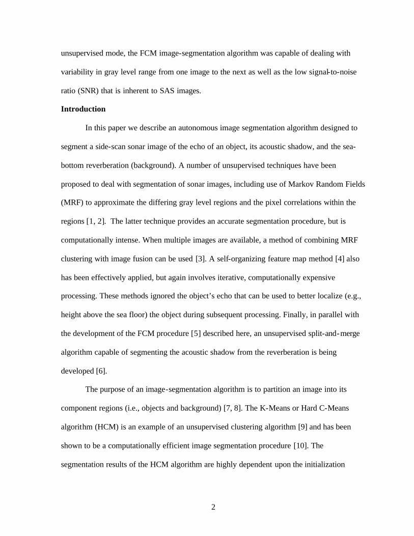
unsupervised mode, the FCM image-segmentation algorithm was capable of dealing with
variability in gray level range from one image to the next as well as the low signal-to-noise
ratio (SNR) that is inherent to SAS images.
Introduction
In this paper we describe an autonomous image segmentation algorithm designed to
segment a side-scan sonar image of the echo of an object, its acoustic shadow, and the sea-
bottom reverberation (background). A number of unsupervised techniques have been
proposed to deal with segmentation of sonar images, including use of Markov Random Fields
(MRF) to approximate the differing gray level regions and the pixel correlations within the
regions [1, 2]. The latter technique provides an accurate segmentation procedure, but is
computationally intense. When multiple images are available, a method of combining MRF
clustering with image fusion can be used [3]. A self-organizing feature map method [4] also
has been effectively applied, but again involves iterative, computationally expensive
processing. These methods ignored the object’s echo that can be used to better localize (e.g.,
height above the sea floor) the object during subsequent processing. Finally, in parallel with
the development of the FCM procedure [5] described here, an unsupervised split-and-merge
algorithm capable of segmenting the acoustic shadow from the reverberation is being
developed [6].
The purpose of an image-segmentation algorithm is to partition an image into its
component regions (i.e., objects and background) [7, 8]. The K-Means or Hard C-Means
algorithm (HCM) is an example of an unsupervised clustering algorithm [9] and has been
shown to be a computationally efficient image segmentation procedure [10]. The
segmentation results of the HCM algorithm are highly dependent upon the initialization

3
resulting in highly variable segmentation due to the local minima of the associated objective
function. This problem was overcome by generalizing the HCM to allow for a fuzzy
membership function for each cluster resulting in the FCM algorithm [10, 11]. The FCM has
been used to implement the image segmentation procedure [11-13]. Further, the FCM
algorithm has been employed in conjunction with multiresolution processing techniques [14]
to solve the problem of shading effects during the segmentation of magnetic resonance
images [15]. Both implementations deal with estimating the number of classes that are
present, an approach that increases the computational complexity of the procedures. In this
application, the procedure is required to estimate three clusters: echo, acoustic-shadow, and
reverberation.
Figure 1 – The SAS images of a cylinder (left) and a spheroid (right). Both objects show the brighter echo of the object itself and larger dark acoustic shadow. Throughout the paper, the eight-bit gray scale of all of the images has been normalized to the range [0, 1] and pseudo-color (color bar on the right) has been applied to enhance the appearance of the images.

4
In our application, image-segmentation serves as a preprocessing step for an object
classification procedure. We expected that the segmentation algorithm would improve the
image SNR prior to the classification module, thereby minimizing the likelihood of
misclassification and maximizing the classifier’s efficacy. Because the first-step in this
procedure extracts a subimage containing the region of interest and discards the bulk of the
pixels that contain no information, the classifier’s computational complexity is reduced.
Figure 1 shows the Synthetic Aperture Sonar (SAS) images of two objects. The
images were simulated using the Shallow Water Acoustics Toolkit (SWAT), which is
available from the Office of Naval Research [16]. All figures are plotted using a linear gray
scale with 256 gray levels. Pseudo-coloring was used to make the images easier to view.
Both images were preprocessed to enhance the gray-scale contrast. The image-segmentation
algorithm must be capable of dealing with variability in gray level range from one image to
the next as well as the low SNR that is inherent to sonar images. In each case, the simulated
range was 20 meters from the platform and the object was floating 0.3 meters above a coarse
sand bottom. Our simulations employed the default horizontal array setting.
Methods
Prior to applying the FCM image segmentation procedures, the original images were
preprocessed to deal with poor contrast and low signal to noise ratio (SNR). Figure 2 shows
the effects of the two preprocessing steps on the image of the cylinder in Figure 1. Figures
2.a, 2.b, and 2.c contain the images of the cylinder at each stage of reprocessing and Figures
2.d, 2.e, and 2.f shows the corresponding gray level histogram. The original image of the
cylinder is shown in the Figure 2.a. Figures 2.b and 2.e show the results of applying a
histogram equalization algorithm to the original image [7, 8].

5
Figure 2 – An illustration of the effects of applying two image processing steps to the
original image of the cylinder shown on the left side of Figure 1. The top row contains the gray scale images at three stages of processing. The bottom row shows the corresponding gray level histograms. Figures 2.a and 2.d contain the unprocessed image and its gray level histogram, respectively. Figures 2.b and 2.e illustrate the improvement following histogram equalization. In Figures 2.c and 2.f, a median filter has been applied to the histogram-equalized image resulting in an improved SNR.
The histogram-equalization algorithm distributed the gray levels within the original image
(Figure 2.d) over the entire gray scale range (Figure 2.e) resulting in an image with an
enhanced contrast (Figure 2.b). The effects of the second filtering stage are shown in Figure
2.c. A five-by-five median filter was applied to the contrast-enhanced image in the second
column [7, 8]. As shown in the gray level histogram in Figure 2.f, the gray level distribution
that is associated with the shadow region (gray level range = [0, 0.25]) is clearly separated
from the reverberation distribution which is located in the gray level range [0.4, 0.8].
6
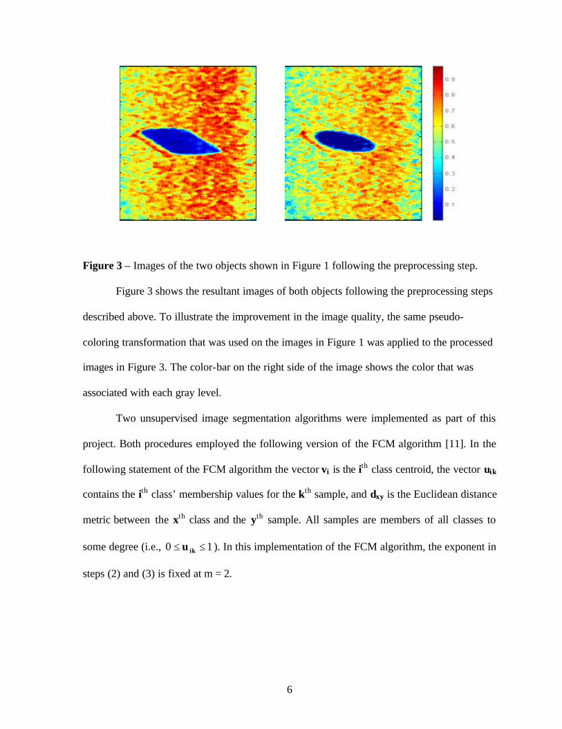
Figure 3 – Images of the two objects shown in Figure 1 following the preprocessing step.
Figure 3 shows the resultant images of both objects following the preprocessing steps
described above. To illustrate the improvement in the image quality, the same pseudo-
coloring transformation that was used on the images in Figure 1 was applied to the processed
images in Figure 3. The color-bar on the right side of the image shows the color that was
associated with each gray level.
Two unsupervised image segmentation algorithms were implemented as part of this
project. Both procedures employed the following version of the FCM algorithm [11]. In the
following statement of the FCM algorithm the vector vi is the ith class centroid, the vector uik
contains the ith class’ membership values for the kth sample, and dxy is the Euclidean distance
metric between the xth class and the yth sample. All samples are members of all classes to
some degree (i.e., 10 ≤≤ iku ). In this implementation of the FCM algorithm, the exponent in
steps (2) and (3) is fixed at m = 2.

7
Fuzzy c-means Algorithm (FCM):
1. Fix the number of clusters, c. Fix m ∞<< m1 . Initialize membership function (MF) U(h=0) to random values. Select metric dik.
2. Calculate the c mean-vectors {vi(h)} using:
( ) ( )∑∑==
=N
1k
mN
1kk
m
i ikik uu xv
3. Update U(h) using: ( )1m2
c
1j jk
ik1h
ik ddu 1
−
=
+ ∑
=
4. Compare U(h) to U(h+1) : if Lε≤− (h)1)(h U- U stop; otherwise h =
h + 1 and go to Step 2.
The HCM is a special case of the FCM clustering technique where the value of the
exponent in step (2) is fixed at m = 1 and the expression in step (3) is replaced by the
following:
(3) ( ) { }
=
= ≤≤+
otherwise,0
,1 dmindu
(h)
jkcj1
(h)
ik1h
ik.
The MFs in the HCM case are actually indicator functions have values of either zero or one.
The first step in our image segmentation process uses the FCM algorithm to extract a
small subimage from the original image by processing both the gray level and location within
the image. Figure 4 illustrates the steps used to implement this procedure, referred to as the
FCM-SIE procedure in the remainder of the discussion. Figure 4.A is a synthesized image
containing a dark region (shadow) in a field of brighter pixels (reverberation). In the first
step, each column of the image was presented to the FCM algorithm as a sample, and each
row was viewed as a feature. The algorithm was initialized to find one class (C = 1). The
8
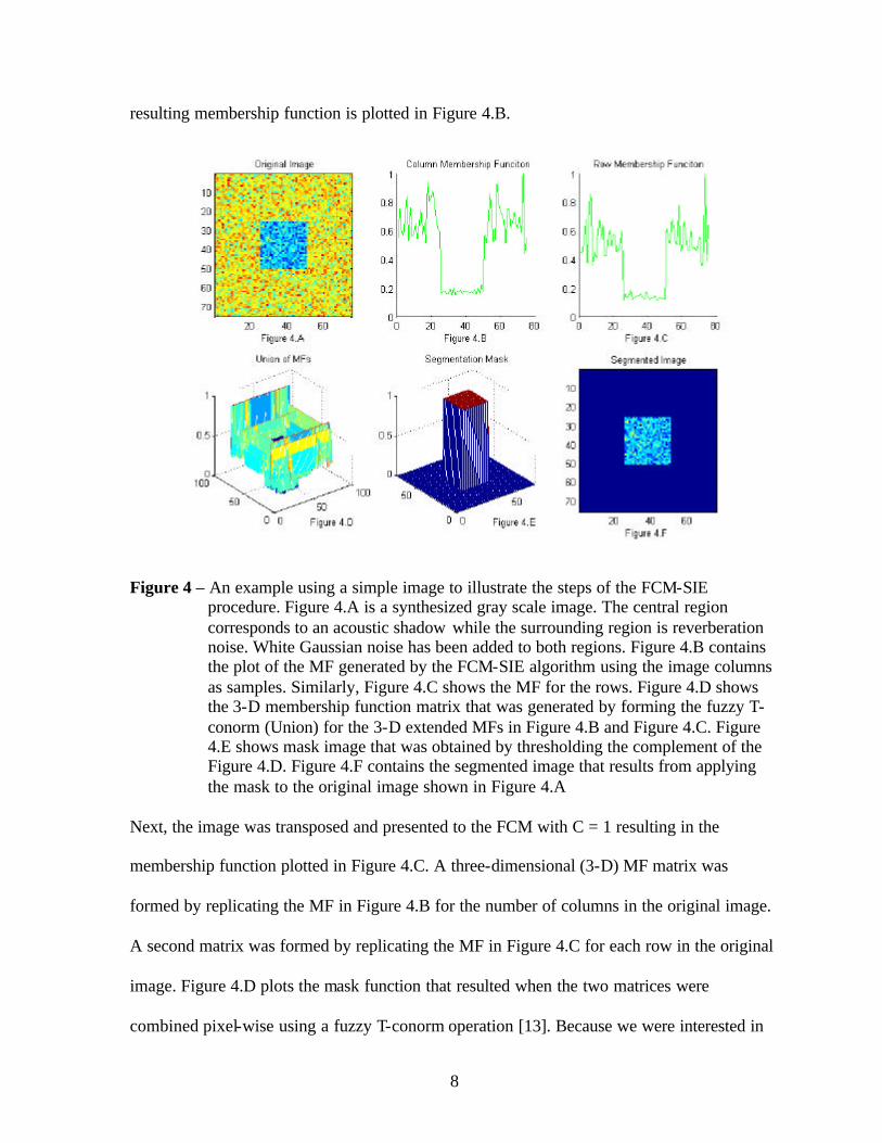
resulting membership function is plotted in Figure 4.B.
Figure 4 – An example using a simple image to illustrate the steps of the FCM-SIE procedure. Figure 4.A is a synthesized gray scale image. The central region corresponds to an acoustic shadow while the surrounding region is reverberation noise. White Gaussian noise has been added to both regions. Figure 4.B contains the plot of the MF generated by the FCM-SIE algorithm using the image columns as samples. Similarly, Figure 4.C shows the MF for the rows. Figure 4.D shows the 3-D membership function matrix that was generated by forming the fuzzy T-conorm (Union) for the 3-D extended MFs in Figure 4.B and Figure 4.C. Figure 4.E shows mask image that was obtained by thresholding the complement of the Figure 4.D. Figure 4.F contains the segmented image that results from applying the mask to the original image shown in Figure 4.A
Next, the image was transposed and presented to the FCM with C = 1 resulting in the
membership function plotted in Figure 4.C. A three-dimensional (3-D) MF matrix was
formed by replicating the MF in Figure 4.B for the number of columns in the original image.
A second matrix was formed by replicating the MF in Figure 4.C for each row in the original
image. Figure 4.D plots the mask function that resulted when the two matrices were
combined pixel-wise using a fuzzy T-conorm operation [13]. Because we were interested in

9
the shadow, the complement of the mask in Figure 4.D was thresholded using the statistics of
the matrix (µ + 1σ), resulting in the binary-valued mask function which is plotted in Figure
4.E. Figure 4.F is the segmented image that resulted from the pixel-wise multiplication of the
original image (Figure 4.A) and the mask shown in Figure 4.E.
Because the segmentation mask is a binary image it can be used to extract the
subimage from the original image. This is accomplished by scanning the mask for pixels
whose gray level is equal to one and saving the corresponding pixel of the original image to
the subimage. Thus, the subimage contained only the pixels within the shadow region
(central square) of in Figure 4.a.
The second step in the image segmentation process employed FCM to segment the
images based of gray level dissimilarities alone. As part of this analysis both the FCM and
the HCM were examined to determine which algorithm performed best for this portion of the
image segmentation task. Throughout the remainder of the discussion these two algorithms
will be referred to as FCM-GLS and HCM-GLS. The segmented images were formed by
assigning to each pixel the weighted value of the MF of the class with the largest degree of
membership. No additional histogram thresholding was employed. Table 1 is a listing of the
acronyms used throughout the remainder of the paper.
Table 1.1 – List of acronyms used through out the following discussion.
FCM Fuzzy C-Means Clustering Algorithm. HCM Hard C-Means Clustering Algorithm (also known as ISODATA, K-Means). FCM-GLS Fuzzy C-Means Gray Level Segmentation procedure. HCM-GLS HCM C-Means Gray Level Segmentation procedure. FCM-SIE Fuzzy C-Means Sub-Image Extraction procedure. MF Membership Function; in the case of HCM the MF reduces to an Indicator
(Characteristic) Function. SNR Signal- to-Noise Ratio. FCM Fuzzy C-Means Clustering Algorithm. SAS Synthetic Aperture Sonar.

10
Results
The FCM-SIE, FCM-GLS, and HCM-GLS procedures were implemented as
MATLAB m-files. The FCM-SIE procedure was presented with the preprocessed images that
were plotted in Figure 3. Figure 5 shows the segmented images that were generated by the
FCM-SIE procedure. The FCM-SIE procedure eliminated large regions of reverberation
noise during the segmentation process. In both cases, the echo and acoustic shadow are
preserved.
Figure 5 – The resulting FCM-SIE segmentations of the cylinder and spheroid objects shown in Figure 1.
The next step in processing involves the gray level segmentation of the subimages
that were extracted the FCM-SIE procedure. The images of both objects were presented to
both the HCM-GLS and the FCM-GLS algorithms multiple times. Each presentation
involved a unique random initialization of the prototypes and membership (indicator)
functions. The HCM-GLS produced substantial variability between the resulting
segmentations due to the presence of local minima within the objective [10].

11
Figure 6 – The subimages 6.a and 6.b were extracted by the FCM-SIE procedure from the original images shown on the top of Figure 1.The FCM-GLS was applied to these subimages with C = 2 classes resulting in the image in Figures 6.c and 6.d Figures 6.e and 6.f show the FCM-GLS results for the three-class (C = 3) segmentation.

12
On the other hand, the FCM-GLS produced very consistent segmentations from one
initialization to the next as a result of the algorithm’s ability to eliminate local minima in the
objective function [11].
The subimages of the cylinder and the spheroid that were extracted by the FCM-SIE
algorithm are shown in Figures 6.a and 6.b, respectively. To further reduce the likelihood of
a misclassification, the FCM-GLS algorithm was applied to these subimages. The results
FCM-GLS image segmentation for the two-class case are shown Figures 6.c and 6.d. The
pixels within the shadow region are clearly segmented from the remaining pixels in both
images resulting in improved contrast and SNR, which in turn improve the likelihood of
correct classification. Figures 6.e and 6.f show the results of the FCM-GLS algorithm for the
three-class case. In both figures, in the region to the left of the shadow, the echo is clearly
segmented from both the reverberation and from the shadow. The shadow itself is also
segmented form the reverberation regions that surround it.
Discussion
The initialization of both the HCM and the FCM required randomized MFs and the
results of the HCM algorithm are highly dependent upon this random initialization. The
function of the HCM-GLS procedure was to assign each pixel of the input image to one of
the C classes. Each class label is associated with one of the standard basis of a C-dimensional
space, termed the label space. The fact that the class label space was discrete induced local
minima in the objective function of the HCM algorithm. Depending upon the initial
conditions, the HCM became stuck in different local minima resulting in highly variable
image segmentation results.
13
The FCM-GLS produced very consistent segmentation results across all repetitions.
The resulting label space for the FCM-GLS is a C-dimensional unit hypercube formed from
the convex hull about the standard basis of the discrete HCM label space. Fuzzification of the
label space increases the uncertainty in the clustering problem, which has the effect of
smoothing out or eliminating the local minima of the objective function. The FCM-GLS does
not become trapped in local minima during the optimization process and thus generates
highly repeatable results.
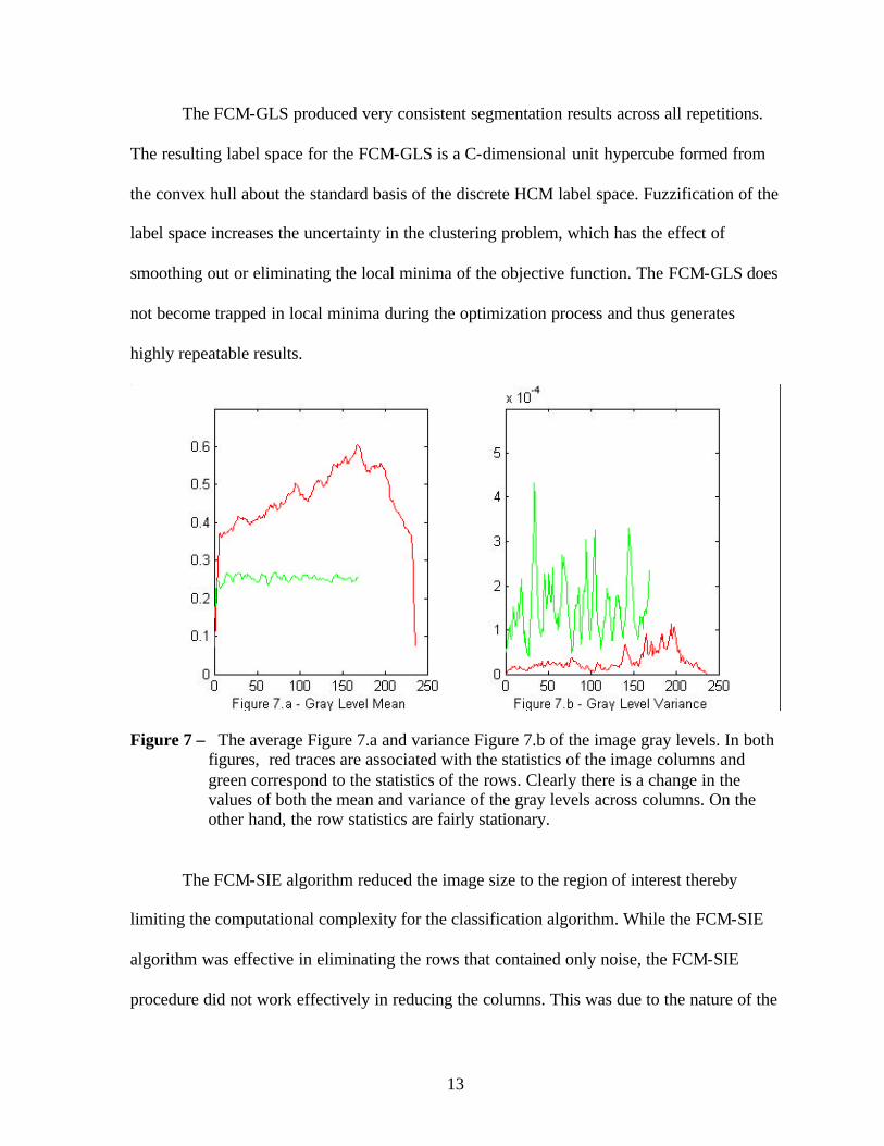
Figure 7 – The average Figure 7.a and variance Figure 7.b of the image gray levels. In both figures, red traces are associated with the statistics of the image columns and green correspond to the statistics of the rows. Clearly there is a change in the values of both the mean and variance of the gray levels across columns. On the other hand, the row statistics are fairly stationary.
The FCM-SIE algorithm reduced the image size to the region of interest thereby
limiting the computational complexity for the classification algorithm. While the FCM-SIE
algorithm was effective in eliminating the rows that contained only noise, the FCM-SIE
procedure did not work effectively in reducing the columns. This was due to the nature of the

14
reverberation noise which was stationary within a given column but which varied along the
rows of the image. Figure 7 shows a plot of the gray level mean and variance for both rows
and columns within a region of the cylinder image that contained only noise. The green plots
show the statistics for each row while the red graphs are plots of the statistics of each
column. The red plots of both in Figures 7.a and 7.b show a change in the level across the
image while the green are, on average, flat. The nonstationary nature of the column statistics
resulted in degraded performance of the FCM-SIE algorithm when the attempt was to reduce
the number of columns in the subimage.
In addition to confounding the FCM-SIE algorithm, the nonstationary nature of the
reverberation also reduced the efficacy of the three-class FCM-GLS. As can be seen in both
Figures 6.e. and 6.f, the reverberation to the left of the shadow region was assigned to the
correct class, while much of the reverberation to the right of the shadow as assigned to the
echo class (red). This misclassification was a direct result of the increasing level of the
reverberation in the region to the right of the shadow.
While the FCM-SIE algorithm, in conjunction with the FCM-GLS, resulted in
consistent gray level image segmentations of the extracted subimages, similar efforts using
the HCM were unsuccessful. Presumably, the HCM-SIE algorithm suffered from the local
minima problem that was present in the HCM-GLS procedure and was further compounded
by the complexity of the input matrix (i.e., both gray level and pixel location were included).
Conclusion
The FCM algorithm was found to be more robust in general than the HCM procedure
when applied to image segmentation. The FCM’s superior performance resulted from the
elimination of local minima in the HCM’s objective function that caused the inconsistent

15
convergence. The FCM-GLS algorithm provided very consistent gray level SAS image
segmentation whereas the HCM-GLS produced highly variable results. The FCM-SIE
procedure further improved the image segmentation by not only improving the contrast of the
segmented image but also by providing the ability to directly extract a subimage that was
significantly smaller in size, thereby decreasing the computational complexity for the
subsequent classification module.
Our future work will involve the development of an adaptive segmentation algorithm
that will be able to employ location information to remove the increasing level of the
reverberation across the columns of the image while preserving the stationary nature of the
noise within the columns. This addition should improve the performance of the FCM-SIE in
extracting a subimage and should result in an improved gray level segmentation by the FCM-
GSL.
Acknowledgement This material is based upon work supported by Mr. Les Jacobi, Code 333, Office of Naval Research,
through the Naval Sea Systems Command under contract No. N00039-97-D-0042, Delivery Order
No. 186.
References
1. Murino, V., Reconstruction and segmentation of underwater acoustic images combining confidence information in MRF models. Pattern Recognition, 2001. 34(5): p. 981-997.
2. Mignotte, M., et al., Sonar image segmentation using an unsupervised hierarchical MRF model. IEEE Transactions on Image Processing, 2000. 9(7): p. 1216 -1231.
3. Hoelscher-Hoebing, U. and D. Kraus, Unsupervised image segmentation and image fusion for multi-beam/multi-aspect sidescan sonar images. OCEANS '98 Conference Proceedings, 1998. 1: p. 571 -576.
4. Yao, K.C., et al., Unsupervised Segmentation using a Self-Organizing Map and a Noise Model Estimation in Sonar Imagery. Pattern Recognition Letters, 2000. 33(9): p. 1575-1584.
16
5. Stitt, J.P., R.L. Tutwiler, and A.S. Lewis, Fuzzy C-Means Image Segmentation of SIde-Scan Sonar Images. Proceedings of 2001 IASTED International Symposium on Signal and Image Processing., 2001.
6. Lewis, A.S., R.L. Tutwiler, and J.P. Stitt, Automatic Parameter Selection for Split/Merge Processing of SIde-Scan Sonar Images. Proceedings of IASTED International Symposium on Measurement and Control., 2001.
7. Gonzalez, R.C. and R.C. Woods, Digital image processing. 1992, Reading, Mass.: Addison-Wesley. xvi, 716 , [8] of plates.
8. Sonka, M., V. Hlavac, and R. Boyle, Image processing, analysis, and machine vision. 2nd ed. 1999, Pacific Grove, CA: PWS Pub. xxiv, 770.
9. Duda, R.O., P.E. Hart, and D.G. Stork, Pattern classification. 2nd ed. 2000, New York: Wiley. xx, 654.
10. Jain, A.K., M.N. Murty, and P.J. Flynn, Data Clustering: A Review. ACM Comput. Surv., 1999. 31(3): p. 264 - 323.
11. Bezdek, J.C., Fuzzy models and algorithms for pattern recognition and image processing. Handbooks of fuzzy sets series ; FSHS 4. 1999, Boston: Kluwer Academic. xv, 776.
12. Bezdek, J.C., Pattern recognition with fuzzy objective function algorithms. Advanced applications in pattern recognition. 1981, New York: Plenum Press. xv, 256.
13. Klir, G.J. and B. Yuan, Fuzzy sets and fuzzy logic: theory and applications. 1995, Upper Saddle River, N.J.: Prentice Hall PTR. xv, 574.
14. Tolias, Y.A. and S.M. Panas, Image Segmentation by a Fuzzy Clustering Algorithm using adaptive spatially constrained membership functions. IEEE Transactions on Systems, Man and Cybernetics, Part A., 1998. 28(3): p. 359 -369.
15. Pham, D.L. and J.L. Prince, An Adaptive Fuzzy C-means algorithm for Image Segmentation in the presence of Intensity Inhomogeneities. Pattern Recognition Letters, 1999. 20(1): p. 57-68.
16. Sammelmann, G.S., Sallow Water Acoustics Toolkit (SWAT). 1997, Office of Naval Research.