Synthetic Aperture Radar Imaging with Motion …math.stanford.edu/~papanico/pubftp/auto.pdfSynthetic...
50
Synthetic Aperture Radar Imaging with Motion Estimation and Autofocus Liliana Borcea * Thomas Callaghan † George Papanicolaou ‡ Abstract We introduce from first principles a synthetic aperture radar (SAR) imaging and target motion estimation method that is combined with compensation for radar platform trajectory perturbations. The main steps of the method are (a) segmentation of the data into properly calibrated small apertures, (b) preliminary motion estimation from the data using the Wigner transform and the ambiguity function, (c) compensation for platform trajectory perturbations using the Wigner transform and the ambiguity function of small aperture preliminary images, and (d) construction of high resolution images over wide apertures using the estimated motion and platform trajectory perturbations. The analysis provides quantitative criteria for imple- menting the aperture segmentation and the parameter estimation process. X-band persistent surveillance SAR is a specific application that is covered by our analysis. Detailed numerical simulations illustrate the robust applicability of the theory and validate the theoretical resolution analysis. 1 Introduction In synthetic aperture radar (SAR) we want to image the reflectivity of a given surface using an antenna system mounted on a platform flying over it, as illustrated in Figure 1. Information about the unknown reflectivity is obtained by emitting periodically at rate Δs probing signals f (t) and recording the echoes D(s, t), indexed by the slow time s of the SAR platform displacement and the fast time t of the probing signal. The slow time parametrizes the location ~ r p (s) of the platform at the instant it emits the signal, and the fast time t runs between two consecutive illuminations (0 <t< Δs). An image is formed by superposing over a platform trajectory segment of arc length (aperture) a, the data D(s, t) match-filtered with the time reversed emitted signal f (t), and back propagated with the round trip travel times τ (s, ~ ρ I ) from the platform to the imaging points ~ ρ I , I (~ ρ I ) = Z S(a) -S(a) ds Z dt D(s, t) f t - τ (s, ~ ρ I ) = Z ωo+πB ωo-πB dω 2π Z S(a) -S(a) ds b f (ω) b D(s, ω)e -iωτ (s,~ ρ I ) . (1.1) * Computational and Applied Mathematics, Rice University, MS 134, Houston, TX 77005-1892. ([email protected]) † Institute for Computational and Mathematical Engineering, Stanford University, Stanford CA 94305. ([email protected]) ‡ Department of Mathematics, Stanford University, Stanford CA 94305. ([email protected]) 1
Transcript of Synthetic Aperture Radar Imaging with Motion …math.stanford.edu/~papanico/pubftp/auto.pdfSynthetic...

Synthetic Aperture Radar Imaging with Motion Estimation and
Autofocus
Liliana Borcea∗ Thomas Callaghan† George Papanicolaou‡
Abstract
We introduce from first principles a synthetic aperture radar (SAR) imaging and targetmotion estimation method that is combined with compensation for radar platform trajectoryperturbations. The main steps of the method are (a) segmentation of the data into properlycalibrated small apertures, (b) preliminary motion estimation from the data using the Wignertransform and the ambiguity function, (c) compensation for platform trajectory perturbationsusing the Wigner transform and the ambiguity function of small aperture preliminary images,and (d) construction of high resolution images over wide apertures using the estimated motionand platform trajectory perturbations. The analysis provides quantitative criteria for imple-menting the aperture segmentation and the parameter estimation process. X-band persistentsurveillance SAR is a specific application that is covered by our analysis. Detailed numericalsimulations illustrate the robust applicability of the theory and validate the theoretical resolutionanalysis.
1 Introduction
In synthetic aperture radar (SAR) we want to image the reflectivity of a given surface using anantenna system mounted on a platform flying over it, as illustrated in Figure 1. Information aboutthe unknown reflectivity is obtained by emitting periodically at rate ∆s probing signals f(t) andrecording the echoes D(s, t), indexed by the slow time s of the SAR platform displacement and thefast time t of the probing signal. The slow time parametrizes the location ~rp(s) of the platformat the instant it emits the signal, and the fast time t runs between two consecutive illuminations(0 < t < ∆s).
An image is formed by superposing over a platform trajectory segment of arc length (aperture)a, the data D(s, t) match-filtered with the time reversed emitted signal f(t), and back propagatedwith the round trip travel times τ(s, ~ρ I) from the platform to the imaging points ~ρ I ,
I(~ρ I) =
∫ S(a)
−S(a)ds
∫dtD(s, t)f
(t− τ(s, ~ρ I)
)=
∫ ωo+πB
ωo−πB
dω
2π
∫ S(a)
−S(a)ds f(ω)D(s, ω)e−iωτ(s,~ρ I). (1.1)
∗Computational and Applied Mathematics, Rice University, MS 134, Houston, TX 77005-1892.([email protected])†Institute for Computational and Mathematical Engineering, Stanford University, Stanford CA 94305.
([email protected])‡Department of Mathematics, Stanford University, Stanford CA 94305. ([email protected])
1

~rp(s)
~ρ Ix
y
z
|~rp(s)− ~ρ I |
Figure 1: Setup for synthetic aperture imaging.
Here hat denotes Fourier transform, the bar stands for complex conjugate, B and ωo are thebandwidth and central frequency of f(t) respectively, S(a) is the slow time range over the apertureof length a, and
τ(s, ~ρ I) = 2|~rp(s)− ~ρ I |/c (1.2)
is the round trip travel time from the platform to the imaging point ~ρ I . The basic theory of SARimaging is presented in [5, 7].
The imaging function (1.1) can be modified in the case of large apertures by introducing aweight factor W (s) that accounts for the geometrical spreading of the wave field over the length ofthe aperture
IW (~ρ I) =
∫ ωo+πB
ωo−πB
dω
2π
∫ S(a)
−S(a)dsW (s)f(ω)D(s, ω)e−iωτ(s,~ρ I). (1.3)
The weight factor is often approximated by W (s) ≈ |~rp(s) − ~ρ I |. It can be calculated exactly inthe case of simple platform trajectories, so that the point spread function is as tight as possible[3, 9, 5].
Our main objective in this paper is to image moving localized reflectors, or targets, that canbe tracked in real time by processing data over sufficiently small sub-apertures. We introducean autofocus process that estimates the SAR platform trajectory perturbations using the Wignertransform and the ambiguity function of small aperture pre-images obtained with (1.1). It is onlyafter the target motion estimation and the autofocus have been carried out that we can computethe final image over a large aperture, using an imaging function like (1.3).
The main steps in the analysis of SAR imaging with motion estimation and autofocus are asfollows. First we segment the data into small apertures and find analytically under what conditionsphases can be linearized so that computationally efficient local Fourier transforms can be used.Next we calculate the ambiguity function of the data over the segmented apertures, and over atime window that is associated with a strong, moving target. Then we show how to estimate incre-mental target motion from estimates of the location of the peaks of the ambiguity function. This
2

includes a sensitivity analysis relative to SAR platform trajectory perturbations. We also analyzethe Wigner transform of the data over segmented apertures, and discuss the relative advantagesand disadvantages of using it rather than the ambiguity function. With the estimates of the targetmotion we construct a preliminary image around the moving target, and then calculate the ambi-guity function and the Wigner transform of this image in a suitable window around its peak. Theambiguity function and the Wigner transform depend on four independent variables. We show howto identify two-dimensional cross sections that contain their peaks. From such estimates of thepeaks we show how, in turn, we can compensate for SAR platform trajectory perturbations. Weuse both the Wigner transform and the ambiguity function because they provide complementaryinformation and with different resolution.
Estimating target motion and compensating for platform trajectory perturbation using theWigner transform and the ambiguity function is the main result of this paper. Alternative ap-proaches to autofocus are given in [8, 6].
Once the motion of the target and the platform trajectory perturbations have been estimatedover successive, overlapping segments of the trajectory, we can form a high resolution image overextended apertures. This approach can be applied to a wide range of SAR imaging systems,including X-band persistent surveillance SAR.
The paper is organized as follows. We begin in Section 2 with a mathematical model of the SARdata and the range compression processing. We also provide a summary of the relevant physicalparameters that are typical in X-band persistent surveillance SAR. In Section 3 we carry out a pre-liminary target motion estimation using the Wigner transform and the ambiguity function directlyon the range compressed data. In Section 4 we analyze the sensitivity of target motion estimationto SAR platform trajectory perturbations. In Section 5 we analyze the Wigner transform and theambiguity function of images. We show how by identifying the peaks in these functions we canestimate parameters that can be used for improving target motion estimation and for compensa-tion for SAR platform trajectory perturbations. In Section 6 we introduce a step-by-step algorithmfor autofocus with motion estimation. In Section 7 we present the results of detailed numericalsimulations, first for target motion estimation alone, and then for SAR platform trajectory pertur-bations without target motion. Even though the theoretical analysis allows for both target motionestimation and for compensation of SAR platform trajectory perturbations, there are a number ofimplementation issues that are addressed in a separate publication. Images must have considerablecomplexity, and processing over several overlapping apertures must be done in a coordinated way,in order to separate target motion estimation from SAR platform trajectory perturbations. Weend in Section 8 with a brief summary and conclusions.
2 Mathematical model of the data
In this section we present a mathematical model for the SAR data, which we use in the analysisof imaging with motion estimation and autofocus. It is based on the single scattering (Born)approximation of the solution of the wave equation, with reflectivity distributed on the surface~x = (x, z = h(x)) in R3, with known elevation z = h(x) at points x ∈ R2. We take for simplicity aflat imaging surface z = 0.
Let s be the time (slow time) that determines the location ~rp(s) of the SAR platform at theinstant it emits the probing signal f(t). We model the data D(s, t) received at the platform over
3

the fast time interval t ∈ (0,∆s) by
D(s, t) ≈ p(t,~rp(s+ t)), (2.1)
where p(t,~r) is the single scattering approximation of the wave field due to the signal f(t) emittedat t = 0 from a point source at ~rp(s). We have
p(t,~r) = −∫dt′∫dx
δ(t− t′ − |~x−~r|/c)4π|~x−~r|
R(t′,x)1
c2
∂2t f(t′ − |~x−~rp(s)|/c)
4π|~x−~rp(s)|, ~x = (x, 0), (2.2)
where
G(t, t′, ~x,~r) =δ(t− t′ − |~x−~r|/c)
4π|~x−~r|is the outgoing Green’s function of the wave equation and R(t,x) is the reflectivity that may changein time due to motion in the imaging region. The emitted signal consists of a base-band waveformfB(t) modulated by a carrier frequency νo = ωo/(2π),
f(t) = e−iωotfB(t), (2.3)
Its Fourier transform is
f(ω) =
∫dt eiωtf(t) = fB(ω − ωo),
and is supported in the interval|ω − ωo| ∈ [−πB, πB] ,
where B is the bandwidth. The probing signals in SAR are often chirps, as described briefly inAppendix A.
To model the time dependent reflectivity R(t,x), let us consider a spotlight SAR mode [7],where the platform steers a narrow radar beam to illuminate continuously the same moving target.We can then model its reflectivity, over a short time t ∈ (0,∆s), by translation from a center point~ρ(s) = (ρ(s), 0), at speed ~u(s) = (u(s), 0) in the imaging plane,
R(t,x) = g(x− ρ(s)− tu(s)). (2.4)
Here g is a function of small compact support around 0, modeling the reflectivity of the target inthe system of coordinates with moving origin ρ(s) + tu(s).
2.1 The X-band SAR regime
Our analysis is based on several approximations that are motivated by specific SAR data regimes.One such regime arises in the GOTCHA Volumetric SAR Data Set [4] for two and three dimensionalX-band persistent surveillance SAR.
The relevant physical parameters in the regime of GOTCHA are as follows. The central fre-quency is ν0 = 9.6Ghz, so that the central wavelength is λo = 3cm. The bandwidth is B = 622MHzsampled with 424 frequencies, so that ∆ν = 1.5MHz. The SAR platform trajectory is assumed tobe circular at height H = 7.3km, with radius R = 7.1km and speed V = 250km/h or 70m/s. Onecircular degree of trajectory is 124m. The pulse repetition rate is 117 per degree, which means thata pulse is sent every 1.05m, and ∆s = 0.015s.
4

We take a typical distance L = 10km to a target, and a typical target speed of |u| = 100km/hor 28m/sec. Then, we have from the basic image resolution theory [5], in ideal scenarios withknown target motion and SAR platform trajectory, that the range resolution of the image (1.1) isc/B = 48cm, and the cross range resolution is λ0L/a = 2.5m, with one degree aperture a.
The GOTCHA regime described here is used in the numerical simulations in Section 7. Theanalysis covers a wider range of parameters, but we keep referring to the GOTCHA parameters forillustration.
2.2 The basic data model
We assume throughout that∗
|~u(s)| . |~V(s)|, where ~V(s) =∂~rp(s+ t)
∂t
∣∣∣∣t=0
, (2.5)
and also that
ωo τ(s, ~ρ(s))|~V(s)|c
=4π|~rp(s)− ~ρ(s)|
λo
|~V(s)|c∼ 1, (2.6)
where λo = c/νo is the central wavelength. Although the platform speed |~V| is much smaller thanthe speed of light c, we consider a high frequency regime with λo |~rp(s)−~ρ(s)|, so that the termsin (2.6) balance each other. We also assume a relatively narrow bandwidth B, satisfying
|~V(s)|c B
νo 1. (2.7)
The bandwidth is narrow because B νo. However, B is sufficiently large so that over the durationO(1/B) of the range compressed signal (see Section 2.4), the platform moves a small distance withrespect to λo,
|~V(s)|B
c
νo= λo.
Let us denote by~ρζ(s) = ~ρ(s) + (ζ, 0)
the points in the support of the reflectivity. We obtain the following result, proved in Appendix B.
Proposition 1 The mathematical model of the fast time Fourier transform of the data
D(s, ω) =
∫dt eiωtD(s, t)
is given approximately by
D(s, ω) ≈ ω2o fB(ω − ωo)eiωoψ(s)
c2
∫dζ
g(ζ)
(4π|~rp(s)− ~ρζ(s)|)2eiωτ(s,~ρζ(s)), (2.8)
where the relative platform and target motion induces an order one Doppler phase ωoψ(s),
ψ(s) =2 (~rp(s)− ~ρ(s))
c·
(~V(s)
c−~u(s)
c
)= τ(s, ~ρ(s))
(~V(s)
c−~u(s)
c
)· ~m(s). (2.9)
∗Assumptions (2.6)-(2.7) hold in GOTCHA: |~V|/c = 2.3·10−7 B/νo = 6.5·10−2 and 4π|~rp − ~ρ|/λo|~V|/c = 0.93.
5

This phase is proportional to the travel time τ(s, ~ρ(s)) and the projection of the relative speed~V(s)− ~u(s) on the unit vector
~m(s) =~rp(s)− ~ρ(s)
|~rp(s)− ~ρ(s)|. (2.10)
2.3 Related data models
At lower frequencies, the Doppler phase ωoψ(s) becomes negligible, and the data model reduces tothe start-stop approximation
D(s, ω) ≈ ω2o fB(ω − ωo)
c2
∫dζ
g(ζ)
(4π|~rp(s)− ~ρζ(s)|)2eiω τ(s,~ρζ(s)), (2.11)
where the platform and target motion can be neglected on the fast time scale.In the case of high frequency (2.6) and broad-band regimes with B ∼ νo, the data model is
D(s, ω) ≈ ω2fB(ω − ωo)eiωψ(s)
c2
∫dζ
g(ζ)
(4π|~rp(s)− ~ρζ(s)|)2eiωτ(s,~ρζ(s)). (2.12)
This is similar to (2.8), except that it involves the Fourier coefficients −ω2fB(ω−ωo) of ∂2t f(t) and
we cannot neglect the variation of the Doppler phase ωψ(s) over the bandwidth.In the case of high frequency (2.6) and very narrow band regimes
B
νo∼ |
~V(s)|c 1,
the data model is
D(s, ω) ≈ ω2o fB [ω(1 + ∆ω)− ωo] eiωoψ(s)
c2
∫dζ
g(ζ)
(4π|~rp(s)− ~ρζ(s)|)2eiωτ(s,~ρζ(s)), (2.13)
where in addition to the Doppler phase ωoψ(s), which is the same as in (2.8), we have the Dopplerfrequency shift by the factor
∆ω =
(~V(s)
c− 2~u(s)
c
)· ~m(s).
We do not analyze here imaging in the broad band or the very narrow band regimes describedabove. We consider only the relatively narrow band regime assumed in Proposition 1, which appliesto a wide range of SAR imaging systems, including the X-band persistent surveillance GOTCHASAR described in section 2.1.
2.4 Range compression
Instead of working directly with the recorded data D(s, t), we compress them by convolution withthe complex conjugate of the time reversed emitted pulse f(−t), offset by the travel time τ(s, ~ρo)to a reference point ~ρo in the imaging plane,
Dr(s, t) =
∫dt′D(s, t′)f (t′ − t− τ(s, ~ρo)). (2.14)
6
In the Fourier domain we have
Dr(s, ω) = fB(ω − ωo)D(s, ω)e−iωτ(s,~ρo)
≈ ω2o
c2
∣∣∣fB(ω − ωo)∣∣∣2 eiωoψ(s)
∫dζ
g(ζ)
(4π|~rp(s)− ~ρζ(s)|)2exp
iω[τ(s, ~ρζ(s))− τ(s, ~ρo)
],
and we make the approximation
|fB(ω − ωo)| ≈ |fB(0)|, for |ω − ωo| ≤ πB, (2.15)
which holds for linear frequency modulated chirps (A.4), or for short pulses f(t) ∼ e−iωotsinc(πBt).We also set the Doppler phase ψ(s) to the constant ψ(0) over the small apertures a used in ourdata processing, because†
ωo [ψ(s)− ψ(0)] ∼ ωosψ′(0) ∼ ωosV2
c2∼ aV
λoc 1, (2.16)
for |s| ≤ S(a) = a/(2V ). The model of Dr(s, ω) becomes
Dr(s, ω) ≈ ω2o |fB(0)|2
c2eiωoψ(0)
∫dζ
g(ζ)
(4π|~rp(s)− ~ρζ(s)|)2exp
iω[τ(s, ~ρζ(s))− τ(s, ~ρo)
]. (2.17)
One advantage of working with range compressed data is that no matter how long is the emittedwaveform f(t), Dr(s, t) behaves like a short pulse with support O(1/B). Another advantage is thatsince its Fourier transform Dr(s, ω) has smaller phases than D(s, ω), it is more convenient innumerical computations.
3 The Wigner transform and ambiguity function of the data
We consider here the Wigner transform and the ambiguity function of the range compressed data,and show how the location of their peaks can be used to estimate the motion of a target. Welimit the discussion at first to the ideal case of perfect knowledge of the SAR platform trajectory.Unavoidable perturbations of this trajectory are considered in Section 4.
Let us suppose that the radar illuminates continuously the same moving target of small support.Idealizing the target by a point at ~ρ(s) = (ρ(s), 0), parametrized by the slow time s, we obtainfrom (2.17) that
Dr(s, ω) ≈ ω2o
c2
∣∣∣fB(0)∣∣∣2 eiωoψ(0)
(4π|~rp(s)− ~ρ(s)|)2exp iω [τ(s, ~ρ(s))− τ(s, ~ρo)] . (3.1)
The platform speed~V(s) = ~r′p(s) = V~t(s), (3.2)
is along the unit vector ~t(s), tangential to the trajectory at ~rp(s). The radius of curvature of thetrajectory is denoted by R and we suppose that
R ∼ |~rp(s)− ~ρ?| ∼ L,†In the GOTCHA regime, at one degree aperture a = 124m, and aV/(λoc) = 9.6 · 10−4.
7

where L is a typical SAR platform-target distance. In reality, the tangential platform speed V andthe radius of curvature R are slowly varying with s, but here we approximate them by constantsover the small time intervals used in the Wigner transform and the ambiguity function. The targetspeed is given by
~u(s) = ~ρ′(s) = (u(s), 0), (3.3)
and u may have arbitrary orientation in the horizontal imaging plane. We assume throughout thepaper that u(s) changes slowly in s, so that we can approximate it by a constant
u(s) ≈ u(0) ≡ u (3.4)
over the slow time interval centered at s = 0, and defining the small apertures used in our dataprocessing.
3.1 The Wigner transform of the SAR data from a point target
The Wigner transform of the range compressed SAR data is given by
W(s,Ω, ω, T ) =
∫ Ω
−Ωdω
∫ S
−Sds Dr
(s+
s
2, ω +
ω
2
)Dr
(s− s
2, ω − ω
2
)eisΩ−iωT , (3.5)
where Ω and T are frequency and time variables, dual to the variables of integration s and ω. Theω integral limit is
Ω = 2πB − 2|ω − ωo|,and it is determined so that ω ± ω/2 remains in the support of Dr for all ω ∈ [−Ω, Ω]. The timeoffset interval s ∈ [−S, S] is chosen in terms of an aperture a measured along the trajectory,
S =a
2V.
We restrict the aperture by asking that the Fresnel number a2/(λoL) satisfy
a2
λoL 4νoV
B|~u|, and
a2
λoL 8LV
a|~u|. (3.6)
We also assume that the reference point ~ρo is close enough to ~ρ(s),
|~ρ(s)− ~ρo| L. (3.7)
Under these conditions we show in Appendix C the following.
Proposition 2 The Wigner transform evaluated at the central frequency ωo has the form
W(s,Ω, ωo, T ) ∼ |fB(0)|4
|~rp(s)− ~ρ(s)|4sinc πB [T − τ(s, ~ρ(s)) + τ(s, ~ρo)]
sinc
2πa
λo
[Ωc
ωoV− 2~u
V· ~m(s) + 2~t(s) · ( ~m(s)− ~mo(s))
], (3.8)
where symbol ∼ stands for approximate, up to a multiplicative constant, ~m(s) is the unit vector in(2.10), and
~mo(s) =~rp(s)− ~ρo|~rp(s)− ~ρo|
. (3.9)
8

Among the two conditions on the Fresnel number in (3.6), the first one is more restrictive. Thisis because typically‡
L
a&νoB 1. (3.10)
The first condition in (3.6) allows us to neglect the quadratic terms s2 in the phase of the integrandin the Wigner transform, and the second condition makes the cubic terms s3 negligible. If werelaxed the assumption (3.6) to
a2
λoL.
4νoV
B|~u|, (3.11)
we would get a more complicated expression of the Wigner transform, involving Fresnel integralsinstead of the sinc functions. However the conclusions drawn below about motion estimation remainthe same, because they only use estimates of the peaks ΩW(s) and TW(s) of W(s,Ω, T, ωo). Thesepeaks are not affected by the quadratic phases in the Fresnel integrals.
3.2 Motion estimation from the peaks of the Wigner transform
It follows from Proposition 2 that from the peaks ΩW(s) and TW(s) of the Wigner transform wecan estimate the travel time τ(s, ~ρ(s)) and the target speed ~u projected along ~m(s). We have
~u
V· ~m(s) =
cΩW(s)
2ωoV+~t(s) · ( ~m(s)− ~mo(s)) +O
(λoa
), (3.12)
and
τ(s, ~ρ(s)) = TW(s) + τ(s, ~ρo) +O
(1
B
). (3.13)
Now, suppose that we have a good estimate of the target location (i.e., of vector ~m(s)), and wewish to estimate its speed ~u, so that we can track it at a later time. Recall that ~u is in the imagingplane, so we can determine it from its projection on two linearly independent vectors in this plane.Equation (3.12) gives only the projection of ~u along the direction ~m(s), when ~m(s) is known. Wecan estimate ~u by solving the nonlinear equation(
~u
V−~t(s+ s)
)· (~rp(s+ s)− ~ρ(s)− s~u)
|~rp(s+ s)− ~ρ(s)− s~u|≈ cΩW(s+ s)
2ωoV−~t(s+ s) · (~rp(s+ s)− ~ρo)
|~rp(s+ s)− ~ρo|
over a small interval of s. This is obtained from (3.12), with tangential platform speed V and ~utreated as constant relative to s. In theory, it is sufficient to take the limit s→ 0, which gives thedifferential form of the nonlinear equation for ~u,∣∣∣∣P(s)
(~t(s)−
~u
V
)∣∣∣∣2 ≈ ∣∣∣Po(s)~t(s)∣∣∣2 |~rp(s)− ~ρ(s)||~rp(s)− ~ρo|
+|~rp(s)− ~ρ(s)|
V~t′(s) · ( ~mo(s)− ~m(s))−
dΩW(s)
ds
c|~rp(s)− ~ρ(s)|2V 2ωo
. (3.14)
Here we letP(s) = I − ~m(s) ( ~m(s))T
‡For GOTCHA, the second condition in (3.6) says a 390m for |~u| = 100km/h. Inequality (3.11), which is therelaxed form of the first condition in (3.6) says a . 219m. Thus, we can work with apertures a ∼ 100m.
9
be the projection on the orthogonal complement of span ~m(s), and used that ~m′(s) =V P(s)(~t(s)−~u/V )|~rp(s)−~ρ(s)| .
Similarly, ~m′o(s) = V Po(s)~t(s)|~rp(s)−~ρo|
, where Po(s) = I − ~mo(s) ( ~mo(s))T .
Equations (3.12) and (3.14) determine ~u · ~m(s) and the norm of P(s)(~t(s) − ~u/V ), from theestimated peaks of the Wigner transform. To get the target speed ~u = (u, 0), we decompose u inthe orthonormal basis m, m⊥, where
m =m
|m|, ~m = (m,mz),
and m⊥ is the unit vector perpendicular to m in the horizontal plane. We know (u ·m), so let usestimate u · m⊥. Since
P(~t−
~u
V
)=(t− u
V−m
(~m ·~t− u ·m
V
), tz −mz
(~m ·~t− u ·m
V
)),
and m is along m, we get ∣∣∣∣t · m⊥ − u · m⊥
V
∣∣∣∣ = η,
where
η =
∣∣∣∣P(~t− ~u
V
)∣∣∣∣2 − [tz −mz
(~m ·~t− u ·m
V
)]2−[(
t− u
V
)· m− |m|
(~m ·~t− u ·m
V
)]21/2
.
This gives the target speed
u =(u ·m)
|m|m +
(t · m⊥ ± η
)m⊥, (3.15)
with an ambiguity in the sign of η in the component of u along m⊥.Note that the target speed estimation described above can be done for a single aperture centered
at s = 0, or for multiple apertures centered at s = [−S, S]. In the latter case, the estimated targetspeed may have some dependence on s, so we can think of (3.15) as giving
u U(s).
Then, we can use these estimates to approximate the target speed by the constant uI , the averageof U(s) over the slow time range [−S, S],
uI =1
2S
∫ S
−SdsU(s). (3.16)
3.3 The ambiguity function of the SAR data from a point target
The ambiguity function of the range compressed SAR data is given by
A(s,Ω, s, T ) =
∫ ωo+πB
ωo−πBdω
∫ S
−Sds Dr
(s+ s+
s
2, ω
)Dr
(s+ s− s
2, ω
)eisΩ−iωT . (3.17)
The slow time window center s and the offset s are independent variables, and Ω and T are the dualvariables of s and ω, respectively. The ambiguity function gives an alternative and complementaryapproach to target motion estimation, as follows from the next Proposition proved in Appendix D.
10

Proposition 3 If we choose S = a/(2V ), with a satisfying (3.6), and if ~ρo is sufficiently close to~ρ(s) for assumption (3.7) to hold, then the ambiguity function evaluated at s = a/(2V ) is givenapproximately by
A(s,Ω,
a
2V, T)∼ |fB(0)|4
|~rp(s)− ~ρ?|4exp
−iωo
[T +
a
c
(~u
V· ~m(s)−~t(s) · ( ~m(s)− ~mo(s))
)]sinc
πB
[T +
a
c
(~u
V· ~m(s)−~t(s) · ( ~m(s)− ~mo(s))
)]
sinc
aΩ
2V− πa2
λo
~t′(s)V· ( ~mo(s)− ~m(s)) +
∣∣∣Po(s)~t(s)∣∣∣2|~rp(s)− ~ρo|
−
∣∣∣P(s)(~t(s)− ~u
V
)∣∣∣2|~rp(s)− ~ρ(s)|
. (3.18)
Thus, the ambiguity function allows us to estimate both the projection of ~u on ~m(s), and thenorm of the projection of the relative speed ~V − ~u on the plane orthogonal to ~m(s). As alreadynoted, in (3.18) we evaluate the ambiguity function at the extreme value of the slow time offsets = a/(2V ). This is to get the tightest second sinc function, which gives the sharpest estimateof the peak ΩA(s) in Ω. This peak and TA(s), the peak of the first sinc in (3.18), determine thetarget speed, up to a sign, without the need for differentiation as in (3.14).
Thus, it appears that the Wigner transform and the ambiguity function provide the sameinformation. However, the precision of the estimated ~u · ~m(s) with the ambiguity function
~u
V· ~m(s) = −cT
A(s)
2SV+~t(s) · ( ~m(s)− ~mo(s)) +O
( c
Ba
)(3.19)
is not as good as in (3.12), becausec
Ba=νoλoBa
λoa.
The estimation of |P(s)(~t(s)−~u/V )| from the Wigner transform requires its peaks ΩW not onlyat s, but in a neighborhood of s, so that we can do the differentiation in (3.14). The ambiguityfunction gives directly∣∣∣∣P(s)
(~t(s)−
~u
V
)∣∣∣∣2 =∣∣∣Po(s)~t(s)∣∣∣2 |~rp(s)− ~ρ(s)|
|~rp(s)− ~ρo|+|~rp(s)− ~ρ(s)|
V~t′(s) · ( ~mo(s)− ~m(s))−
ΩA(s)
s
c|~rp(s)− ~ρ(s)|2ωoV 2
+O
(λoL
a2
), (3.20)
without any need to differentiate. In comparing this estimate with (3.14), we note that they coincideif we replace in (3.14) dΩW(s)/ds by ΩA(s)/s. We also note that because of our aperture limitationassumption (3.11), the estimates are useful if we have a large Fresnel number§
1 a2
λoL.
4νoV
B|~u|. (3.21)
This means that the aperture a cannot be too small if the motion estimation is to work. It mustbe large enough, but still limited by (3.21).
§In the GOTCHA regime, the Fresnel number is a2/(λoL) = 49 for a one degree aperture and 4νoV/(B|~u|) = 154.
11

3.4 Comparison of motion estimation with the Wigner transform and with theambiguity function
The peak of the Wigner transform (3.8) in the T variable can be used to estimate the round triptravel time τ(s, ~ρ(s)) to the moving target. There is only one peak if there is only one target as in(3.8). In general, there will be many peaks, each associated with a different target. The Wignerdistribution can, therefore, be used to select a time window associated with a target whose motionwe want to estimate. This windowing must be done before computing the ambiguity function(3.18). That is, the data D(s, t) must be windowed in t, after range compression, around the roundtrip travel time from the target of interest. Its Fourier transform is then used to compute theambiguity function (3.17).
It appears from this observation that the peaks of the Wigner transform have all the relevantinformation for motion estimation, allowing for the differentiation with respect to the slow time sthat gives (3.14). The computation of the ambiguity function seems to be superfluous at this point.However, as noted in the previous Section, the peaks of the ambiguity function provide directly,in (3.20), the information that is obtained by differentiation of the peak location of the Wignertransform. Avoiding differentiation with respect to the slow time s is important when dealing withnoisy data. We see therefore that the ambiguity function may provide a more robust estimate of|P(~t− ~u/V )|. But we also need the Wigner transform for windowing, as noted already.
3.5 Sensitivity of target motion estimation to knowledge of its initial location
The estimation of ~u from (3.12), (3.15) and (3.20) requires the vector ~m(s) in (2.10), and the targetrange |~rp(s)−~ρ(s)|. Neglecting the SAR platform trajectory perturbations, the range is determinedwith resolution c/B from the travel time τ(s, ~ρ(s)), which is estimated from the Wigner transform.The target location cannot be estimated directly from the data, before forming an image, butwe suppose that we know an approximation ~ρ? of ~ρ(s), either from direct observations, or fromtracking the target at previous times. That is, we approximate ~m(s) by ~m?(s) in (3.9), with
~m?(s) =~rp(s)− ~ρ?(s)|~rp(s)− ~ρ?(s)|
and ~ρ? in the imaging plane, at distance c/2τ(s, ~ρ(s)) from ~rp(s). In this Section we quantify thesensitivity of the target motion estimation to the error ~ρ− ~ρ? in the target location.
Let ∆~u = (∆u, 0) be the error in the velocity estimation. We obtain from (3.12) that
(~u + ∆~u) · ~m?
V=
cΩW
2ωoV+~t · ( ~m? − ~mo) =
~u · ~m?
V+
(~t−
~u
V
)· ( ~m? − ~m) +O
(λoa
),
and therefore
∆~u · ~m?
V=
(~t−
~u
V
)· ( ~m? − ~m) +O
(λoa
)= O
(|~ρ− ~ρ?|
L
)+O
(λoa
). (3.22)
Similarly, the error of the estimate (3.19) from the ambiguity function is
∆~u · ~m?
V= O
(|~ρ− ~ρ?|
L
)+O
( c
Ba
), (3.23)
12

and it is comparable to (3.22) when
|~ρ− ~ρ?|L
&c
Ba λo
a.
Thus, we need a more precise target location |~ρ(s)−~ρ?(s)| ∼ λoL/a in order to gain accuracy fromthe Wigner transform estimate.
From (3.20) we have that∣∣∣∣P?(~t− ~u + ∆~u
V
)∣∣∣∣2 =
∣∣∣∣P(~t− ~u
V
)∣∣∣∣2 +|~rp − ~ρ|V
~t′ · ( ~m− ~m?) +O
(λoL
a2
)=
∣∣∣∣P(~t− ~u
V
)∣∣∣∣2 +O
(|~ρ− ~ρ?|
L+λoL
a2
), (3.24)
because |~t′| = V/R ∼ V/|~rp − ~ρ|. The second term in the error dominates the first because of thesecond assumption in (3.6), provided that |~ρ− ~ρ?| . a. In view of (3.11) and for |~u| . V we have
|~ρ− ~ρ?|L
.a
L.νoλoBa
=c
Ba.λoL
a2.
We conclude that the velocity estimation with the ambiguity function is insensitive to the choiceof the reference point ~ρ?, as long as |~ρ(s)− ~ρ?| . a. The Wigner transform gives the same resultsas the ambiguity function in general, for |~ρ − ~ρ?| . a. However, when ~ρ? is closer to ~ρ, so that|~ρ? − ~ρ| is comparable to the cross range resolution λoL/a, the Wigner transform gives a sharperestimate of ~u · ~m(s). The importance of this observation will become clear in Section 5, wherewe study how the errors in the motion estimation and the SAR platform trajectory perturbationsaffect the peaks of preliminary images formed over the small aperture a.
4 Motion estimation with SAR platform trajectory perturbations
The SAR platform trajectory is known only approximately. We therefore consider perturbations~µ(s) of ~rp(s),
~rp(s)→ ~rp(s) + ~µ(s)
and rewrite the range compressed data (3.1) in the form
Dr(s, ω) ≈ ω2o
c2
∣∣∣fB(0)∣∣∣2 eiωoψ(0)
(4π|~rp(s)− ~ρ(s)|)2exp
2iω
c(|~rp(s) + ~µ(s)− ~ρ(s)| − |~rp(s)− ~ρo|)
. (4.1)
We assume that the SAR platform trajectory perturbations vary on the slow scale s and are small,so that only the unperturbed platform speed appears in the Doppler phase ψ in (2.9). This isbecause ωoψ ∼ 1 by assumption (2.6), and therefore perturbations of ψ are negligible. The effectof ~µ(s) on the amplitude of Dr(s, ω) is negligible as well.
In this Section we quantify the sensitivity of motion estimation to the platform trajectoryperturbations ~µ(s). We begin in the next section with assumptions on ~µ(s). The results of thesensitivity analysis are in Section 4.2.
13

4.1 Assumptions about the SAR platform trajectory perturbations
Let us begin by writing the range compressed data in the time domain in the form
Dr(s, t) ≈ω2o
c2
∣∣∣fB(0)∣∣∣2 eiωoψ(0)
(4π|~rp(s)− ~ρ(s)|)2
× exp
2iωoc
[|~rp(s)− ~ρ(s)| − |~rp(s)− ~ρo|+ ~µ(s) · ~m(s) +O
(|~µ(s)|2
L
)]×sinc
2πB
c
[|~rp(s)− ~ρ(s)| − |~rp(s)− ~ρo|+ ~µ(s) · ~m(s) +O
(|~µ(s)|2
L
)], (4.2)
where ~m(s) is given by (2.10). The residual in the phase can be neglected under the assumption¶
|~µ(s)| √λoL, (4.3)
which implies that it can be neglected in the sinc function as well.The trajectory perturbations ~µ(s) induce perturbations ~m(s) · ~µ(s)/c of the travel time which
can, in principle, be detected and compensated directly from the traces, with resolution O(1/B),when the perturbations are large enough
| ~m(s) · ~µ(s)| O( cB
).
By compensation, we mean that we can estimate ~m(s) · ~µ(s) and replace in all the subsequentprocessing the ideal platform locations ~rp(s) by ~rp(s) + ( ~m(s) · ~µ(s)) ~m(s). We assume from nowon that such a compensation has been made.
We now introduce some simple, conservative bounds on the norm of the trajectory perturbation~µ and its derivatives with respect to the slow time s. They are conservative in the sense that theyare sufficient for the sensitivity analysis of the next section and for the autofocus analysis presentedin Section 5.
We assume in (4.3) that the norm of the trajectory perturbations is bounded by
|~µ(s)| ∼ µ√λoL a, (4.4)
with the second inequality being a consequence of the smallness of the inverse Fresnel numberλoL/a
2 1 in (3.21). The speed of the trajectory perturbation |~µ′(s)| should be a small fractionof V . We scale it relative to the inverse of the Fresnel number, using a dimensionless parameter δ,so that
a∣∣~µ′(s)∣∣V
∼ λoL
aδ a. (4.5)
For the sensitivity analysis that follows, we assume that δ satisfies
δ λoL
a2and δ µ
a. (4.6)
The first inequality implies, along with (3.11), that
δ B
νo, (4.7)
¶For GOTCHA, this bound is |~µ(s)| 17m.
14

for target speeds |~u| . V .We assume that the acceleration of the trajectory perturbation satisfies
a2|~µ′′(s)|V 2
∼ λoγ λoL
a, (4.8)
where we have introduced another dimensionless parameter γ. For the sensitivity analysis weassume that γ a/L.
We finally assume thata3|~µ′′′(s)|
V 3 λo, (4.9)
so that we can approximate ~µ(s) by a second degree polynomial in s over the small aperture usedin the motion estimation.
It is convenient in the sensitivity analysis to assume that
γ ∼ δ (4.10)
so that we can work with the single dimensionless parameter
ε = min1, γ, δ. (4.11)
According to (4.6) and (4.7), it satisfies‖
ε λoL
a2, ε B
νoand ε µ
a. (4.12)
This allows us to express the Wigner transforms and the ambiguity functions in terms of sincs,rather than Fresnel integrals.
4.2 Sensitivity of motion estimation to SAR platform trajectory perturbations
With the scaling introduced above, we obtain the following results proved in Appendix E.
Theorem 1 The Wigner transform of the range compressed data takes the form
W(s,Ω, ωo, T ) ∼ |fB(0)|4
|~rp(s)− ~ρ(s)|4sinc
πB[T + δTW − τ(s, ~ρ(s)) + τ(s, ~ρo)
]sinc
2πa
λo
[c(Ω + δΩW)
V ωo− 2~u
V· ~m(s) + 2~t(s) · ( ~m(s)− ~mo(s))
],
where
δTW =2~µ(s) · ~m(s)
c, and
cδΩW
V ωo=~µ′(s)
V· ~m(s) +
(~t(s)−
~u
V
)· P(s)~µ(s)
|~rp(s)− ~ρ(s)|.
‖In the GOTCHA regime, at one degree aperture a = 124m we have λoL/a2 = 0.02, B/νo = 0.06 and so we can
work with ε & 0.3. This gives in (4.5) |~µ′|/V . 0.1, i.e. |~µ′| . 25km/h and in (4.8) |~µ′′| . 0.05m/s2. When we lookat the proof in Appendix E, we see that we have completely ignored the multiplicative constants and that, in fact,the results hold for accelerations that can be about 20 times larger than this. The same multiplicative constant canbe applied to |~µ′′′|.
15
Theorem 2 The ambiguity function evaluated at s = a/(2V ) has the form
A(s,Ω,
a
2V, T)∼ |fB(0)|4
|~rp(s)− ~ρ(s)|4e−iωo[T+δTA−a
c [~t(s)·( ~m(s)− ~mo(s))− ~uV· ~m(s)]]
sinc
πB
[T + δTA − a
c
[~t(s) · ( ~m(s)− ~mo(s))−
~u
V· ~m(s)
]]
sinc
a(Ω + δΩA)
2V− πa2
λo
~t′(s)V· ( ~mo(s)− ~m(s)) +
∣∣∣Po(s)~t(s)∣∣∣2|~rp(s)− ~ρo|
−
∣∣∣P(s)(~t(s)− ~u
V
)∣∣∣2|~rp(s)− ~ρ(s)|
,
where
δTA = − aV
δΩW
ωoand
δΩA
ωo=V a
c
2(~t− ~u
V
)|~rp(s)− ~ρ(s)|
· P(s)~µ′(s)
V−~µ′′(s)
V 2· ~m(s)
.We conclude from Theorem 1 that the platform perturbations induce an error ∼ ~µ(s) · ~m(s)/c
in the travel time estimation with the Wigner transform. As explained in the beginning of theprevious section, this perturbation is within the main lobe of the first sinc function in W, withresolution O(1/B). It has therefore a small effect on the travel time estimation. However, thetarget motion estimation is affected by the platform trajectory perturbations. Explicitly, we havethe errors
cδΩW
V ωo= O
(|~µ′(s) · ~m(s)|
V+|~µ(s)|L
)= O
(λoL
a2ε+µ
L
)(4.13)
in the estimation of ~u/V · ~m(s), and errors
cδΩA
V aωo= O
(∣∣∣∣P(s)~µ′(s)
V
∣∣∣∣+L|~µ′′(s) · ~m(s)|
V 2
)∼ O
(λoL
a2ε
)(4.14)
in the estimation of |P(s)(~t(s)− ~u/V )|2.Recalling from Section 3.3 that λoL/a
2 is the error bound on the estimated |~u|/V with theunperturbed platform trajectory, we can conclude that we can only approximate the target speed~u by ~uI , with an error
|∆~u|V.λoL
a2ε, where ∆~u = ~uI − ~u , (4.15)
with ε defined by (4.11).
5 Images, their ambiguity function and autofocus
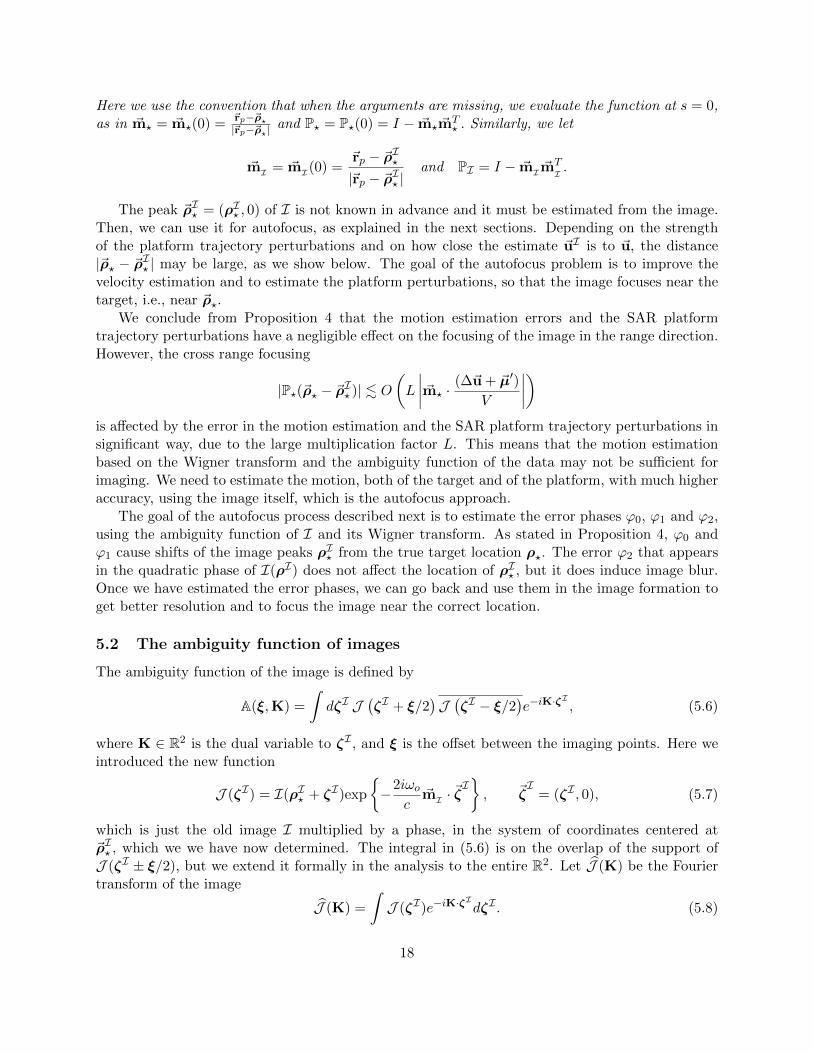
We first quantify in Section 5.1 the effect of SAR platform perturbations on the location of peaksof preliminary images obtained with small apertures. Then, we form in Sections 5.2 and 5.3 theambiguity function and the Wigner transform of these images, and analyze how SAR platformperturbations influence the location of their peaks. We also show in Section 5.4 how to estimateparameters associated with platform perturbations, so that they can be used in sharpening theimage, formed over wider apertures. This is the autofocus process. We assume here that motion
16
estimation from the data, as described in the previous sections, has been carried out. An algorithmfor both motion estimation and autofocus, based on our analysis, is presented in Section 6. Forsimplicity, we take the case of a point target. The results extend qualitatively to targets of finitesupport, although the analysis is more tedious.
5.1 Preliminary images with small apertures
Let us begin by rewriting the imaging function (1.1) in terms of the range compressed data
I(ρI) =
∫ S
−Sds
∫ ωo+πB
ωo−πB
dω
2πDr(s, ω)e−
2iωc (|~rp(s)−~ρ I−s~uI |−|~rp(s)−~ρo|), (5.1)
where ~ρ I = (ρI , 0) is the search point in the horizontal image plane and ~uI is the estimated targetspeed. We denote by ~ρ? = (ρ?, 0) the true target location at s = 0, the center of the aperture,assuming that it is in uniform translational motion over the slow time range |s| ≤ S = a/(2V ) thatdefines the small aperture a,
~ρ(s) = ~ρ? + s~u. (5.2)
For the analysis we use the range compressed data model (4.1). The focusing of the preliminaryimage I(ρI) is described in Proposition 4 whose proof is in Appendix F. We assume the sameconstraints on the aperture as in Propositions 2 and 3, and also those on the platform trajectoryperturbations ~µ(s) described in Section 3.
Proposition 4 The image I(ρI) is given by
I(ρI) ∼∫ ωo+πB
ωo−πBdω exp
2iω
c
(|~rp − ~ρ?| − |~rp − ~ρI? |+ ϕ0
)∫ S
−Sds
exp
2iωsV
c
[(~t−
~uI
V
)· ( ~m? − ~mI ) + ϕ1
]+iωo(sV )2
cϕ2
, (5.3)
where
ϕo = ~m? · ~µ,
ϕ1 = ~m? ·(∆~u + ~µ′)
V+
(~t−
~uI
V
)· P?~µ|~rp − ~ρ?|
,
ϕ2 =~µ′′ · ~m?
V 2+~t′
V· ( ~m? − ~mI ) +
∣∣∣P? (~t− ~uI
V + ∆~u+~µ′
V
)∣∣∣2|~rp − ~ρ?|
−
∣∣∣PI (~t− ~uI
V
)∣∣∣2|~rp − ~ρI? |
and ~ρI? = (ρI? , 0) is the image peak. It satisfies∣∣∣ ~m? · (~ρ? − ~ρI? )∣∣∣ = O(ϕ0) . O
( cB
)(5.4)
and ∣∣∣∣∣(~t−
~uI
V
)· P?(
~ρ? − ~ρI? )
|~rp − ~ρ?|
∣∣∣∣∣ = O(ϕ1) ∼ λoL
a2ε. (5.5)
17
Here we use the convention that when the arguments are missing, we evaluate the function at s = 0,as in ~m? = ~m?(0) =
~rp−~ρ?|~rp−~ρ?|
and P? = P?(0) = I − ~m? ~mT? . Similarly, we let
~mI = ~mI (0) =~rp − ~ρI?|~rp − ~ρI? |
and PI = I − ~mI ~mTI .
The peak ~ρI? = (ρI? , 0) of I is not known in advance and it must be estimated from the image.Then, we can use it for autofocus, as explained in the next sections. Depending on the strengthof the platform trajectory perturbations and on how close the estimate ~uI is to ~u, the distance|~ρ? − ~ρI? | may be large, as we show below. The goal of the autofocus problem is to improve thevelocity estimation and to estimate the platform perturbations, so that the image focuses near thetarget, i.e., near ~ρ?.
We conclude from Proposition 4 that the motion estimation errors and the SAR platformtrajectory perturbations have a negligible effect on the focusing of the image in the range direction.However, the cross range focusing
|P?(~ρ? − ~ρI? )| . O(L
∣∣∣∣ ~m? ·(∆~u + ~µ′)
V
∣∣∣∣)is affected by the error in the motion estimation and the SAR platform trajectory perturbations insignificant way, due to the large multiplication factor L. This means that the motion estimationbased on the Wigner transform and the ambiguity function of the data may not be sufficient forimaging. We need to estimate the motion, both of the target and of the platform, with much higheraccuracy, using the image itself, which is the autofocus approach.
The goal of the autofocus process described next is to estimate the error phases ϕ0, ϕ1 and ϕ2,using the ambiguity function of I and its Wigner transform. As stated in Proposition 4, ϕ0 andϕ1 cause shifts of the image peaks ρI? from the true target location ρ?. The error ϕ2 that appearsin the quadratic phase of I(ρI) does not affect the location of ρI? , but it does induce image blur.Once we have estimated the error phases, we can go back and use them in the image formation toget better resolution and to focus the image near the correct location.
5.2 The ambiguity function of images
The ambiguity function of the image is defined by
A(ξ,K) =
∫dζI J
(ζI + ξ/2
)J(ζI − ξ/2
)e−iK·ζ
I, (5.6)
where K ∈ R2 is the dual variable to ζI , and ξ is the offset between the imaging points. Here weintroduced the new function
J (ζI) = I(ρI? + ζI)exp
−2iωo
c~mI · ~ζ
I, ~ζ
I= (ζI , 0), (5.7)
which is just the old image I multiplied by a phase, in the system of coordinates centered at~ρI? , which we we have now determined. The integral in (5.6) is on the overlap of the support ofJ (ζI ± ξ/2), but we extend it formally in the analysis to the entire R2. Let J (K) be the Fouriertransform of the image
J (K) =
∫J (ζI)e−iK·ζ
IdζI . (5.8)
18

Then, the ambiguity function has the following form in terms of the Fourier transform of J ,
A(ξ,K) =1
(2π)2
∫dK J
(K + K/2
)J(K−K/2
)eiK·ξ. (5.9)
To state our result on the form of A(ξ,K), let us introduce the following notation. We let
~mI =~rp − ~ρI?|~rp − ~ρI? |
be the unit vector pointing from the platform to the peak of the image, and mI its projection onthe imaging plane. We also let PI = I − ~mI ~m
TI be the projection on the orthogonal complement
of span ~mI, and denote by
PpI
(~t−
~uI
V
)=
(t− uI
V
)−mI
[~mI ·
(~t−
~uI
V
)](5.10)
the projection of PI(~t− ~uI
V
)in the horizontal plane.
Under the same assumptions as in Proposition 4, and assuming further that the vector in (5.10)is not collinear with mI , we obtain the following result, proved in Appendix G.
Theorem 3 The ambiguity function of the image of a point target at ~ρ? is given by
A(ξ,K) ∼ exp
2iω(K)
c
(|~rp − ~ρ?| − |~rp − ~ρI? |+ ϕ0
)+
2iωos(K)V
cΦ1
sinc
2πB
c
(1− |ω(K)|
2πB
)[mI · ξ + s(K)V Φ1]
sinc
2πa(
1− V |s(K)|a
)λo
ξ · PpI(~t− ~uI
V
)|~rp − ~ρI? |
+ω(K)
ωoΦ1 + s(K)V ϕ2
,
where ∼ denotes approximation up to a multiplicative constant, and s(K) and ω(K) are defineduniquely in terms of the dual variable K, by equation
K =2ω
cmI +
2ωosV
c
PpI(~t− ~uI
V
)|~rp − ~ρI? |
, |s|V ≤ a, |ω| ≤ 2πB, (5.11)
and
Φ1 = ϕ1 +
(~t−
~uI
V
)· ( ~m? − ~mI ). (5.12)
5.3 The Wigner transform of images
The Wigner transform of the image is given by
W(ζI ,K) =
∫dξJ
(ζI + ξ/2
)J(ζI − ξ/2
)e−iK·ξ, (5.13)
19

where K ∈ R2 is the dual variable to ξ, and ζI is the imaging point offset from the peak ~ρI? ofthe image. The integral in (5.6) is on the overlap of the support of J (ζI ± ξ/2), but we extend itformally in the analysis to the entire R2. As we have done in Section (5.2), we can write W(ζI ,K)in terms of the Fourier transform J (K) of the image
W(ζI ,K) =1
(2π)2
∫dK J
(K + K/2
)J(K− K/2
)eiK·ζ
I. (5.14)
Moreover, under the same assumptions as in Theorem 3, we obtain the following form of the Wignertransform.
Theorem 4 The Wigner transform of the image of a point target at ~ρ? is given by
W(ζI ,K) ∼ sinc
4 (πB − |ω(K)− ωo|)
c
[mI · ζ
I + |~rp − ~ρ?| − |~rp − ~ρI? |+ ϕ0 + s(K)V Φ1
]
sinc
2ωoa(
1− 2V |s(K)|a
)c
ζI · PpI(~t− ~uI
V
)|~rp − ~ρI? |
+ω(K)
ωoΦ1 + s(K)V ϕ2
,
where ∼ denotes approximation up to a multiplicative constant, and s(K) and ω(K) are defineduniquely in terms of the dual variable K by equation
K =2(ω − ωo)
cmI +
2ωosV
c
PpI(~t− ~uI
V
)|~rp − ~ρI? |
. (5.15)
5.4 Autofocus: estimating effects of platform trajectory perturbations
Now, let us explain how we can use Theorems 3 and 4 to determine the platform perturbationterms that affect the velocity estimation and the imaging process. The autofocus requires that weknow ρ?, the true location of the target at s = 0, corresponding to the center of the aperture. Thegoal is to estimate the error terms ϕ0, ϕ1 and ϕ2, and then use them to improve the image.
5.5 Estimation of the error phase terms from the ambiguity function and theWigner transform of the image
The peaks of the ambiguity function A(ξ,K) depend only on the error terms ϕ1 and ϕ2. The errorϕ0 appears in the phase of A, which may be tricky to estimate. However, we can determine it fromthe peaks of the Wigner transform, as we show further down. Let us evaluate A(ξ,K) at
K = Ks =ωoa
c
PpI(~t− ~uI
V
)|~rp − ~ρI? |
, (5.16)
and obtain from (5.11) that
ω(Ks) = 0, s(Ks) =a
2V.
With this K, we get from Theorem 3 that
A(ξ,Ks) ∼ eiωoc
Φ1sinc
2πB
c
[mI · ξ +
a
2Φ1
]sinc
πaλoξ · PpI
(~t− ~uI
V
)|~rp − ~ρI? |
+a
2ϕ2
. (5.17)
20

If we let ξ(Ks) be the peak of this function, we have
ϕ1 = ϕA1
+O( c
aB
)ϕA
1=
(~t−
~uI
V
)· ( ~mI − ~m?)−mI ·
ξ(Ks)
a(5.18)
and
ϕ2 = ϕA2
+O
(λoa2
)ϕA
2= − 2ξ(Ks)
a|~rp − ~ρI? |· PI
(~t−
~uI
V
). (5.19)
The peaks of the Wigner transform given in Theorem 4 determine all three error terms ϕ0, ϕ1
and ϕ2. Explicitly, if we evaluate W(ζI ,K) at the dual variable
K = Kω =πB
cmI , (5.20)
we obtain from (5.15) that
ω(K) = ωo +πB
2, s(K) = 0.
The Wigner transform evaluated at K = Kω is
W(ζI ,Kω) ∼ sinc
2πB
c
[mI · ζ
I + |~rp − ~ρ?| − |~rp − ~ρI? |+ ϕ0
]sinc
2ωoa
c
ζI · PpI(~t− ~uI
V
)|~rp − ~ρI? |
+ Φ1
,
and it peaks at ζI(Kω). Therefore, we can estimate
ϕ1 = ϕW1
+O
(λo2a
)
ϕW1
=
(~t−
~uI
V
)· ( ~mI − ~m?)− ζI(Kω) ·
PpI(~t− ~uI
V
)|~rp − ~ρI? |
. (5.21)
This is a more accurate estimate of ϕ1 than that in (5.18), because the additional perturbation termin (5.21) is much smaller than the resolution limit c/(aB) in (5.18). This observation is important,because as we saw in Proposition 4, it is the term ~m? · (∆~u + ~µ′)/V that affects most strongly theoffset of the peak ~ρI? of the image from ~ρ?, in the cross range direction.
The remaining SAR platform perturbation term ϕ0 is
ϕ0 = ϕW0 +O
( c
2B
)ϕW
0 = −mI · ζI(Ks) + |~rp − ~ρI? | − |~rp − ~ρ?|. (5.22)
Getting the same perturbation from the ambiguity function requires the estimation of its phase,which may be difficult to implement in practice. Moreover, to get the analogue of (5.19), we canevaluate the Wigner transform at
K = Ks =2ωoc
mI +ωoa
2c
PpI(~t− ~uI
V
)|~rp − ~ρI? |
21
so that (5.15) gives
ω(Ks) = ωo, s(Ks) =a
4V
and so
ϕ2 = ϕW2
+O
(λoa2
)ϕW
2= − 4ζI(Ks)
a|~rp − ~ρI? |· PI
(~t−
~uI
V
). (5.23)
However, there is no gain in the estimation of ϕ2 from the peak ζI(Ks) of W (ζI ,Ks), because theresolution O(λo/a
2) is the same as that in (5.19).
6 The autofocus algorithm with motion estimation
The analysis that we have carried out in the previous sections suggest a step-by-step algorithm for(a) target motion estimation, (b) platform trajectory perturbation estimation and (c) formationof high-resolution images over extended apertures. We present here a basic algorithm that candeal with either (a) or (b), that is, it cannot deal directly with both target motion estimationand trajectory platform perturbations. To do a combined target motion and platform trajectoryperturbation requires more complex scenes of reference targets that move with different speeds,and estimation over several overlapping apertures. The algorithm presented here is a componentin a more elaborate strategy for combined target motion-platform trajectory estimation, which willbe presented elsewhere.
• Preliminary motion estimation
Step 1. Range-compress the data as in Section 2.4.
Step 2. Compute the Wigner transform of the range compressed data (3.5) as a two-dimensional Fourier transform for each s ∈ [−S, S]. Using the peak of the Wigner transformin Ω for each s, estimate ~u · ~m(s) as in (3.12).
Step 3. Compute the ambiguity function (3.17) as a two-dimensional Fourier transformfor each s ∈ [−S, S]. Estimate its peak as a function of Ω. From this, estimate further, as in(3.20), the component of the motion orthogonal to ~m.
Step 4. Combine these estimates to compute the estimate uI of the target speed, as inequation (3.15). Here, we can use a single aperture centered at slow time s = 0, or we mayuse multiple apertures centered at s ∈ [−S, S]. In the latter case, the target speed estimatesmay depend on s, and we denote them by U(s). Then, we obtain uI by averaging U(s) overthe aperture, as in (3.16).
• Improved target motion estimation or autofocus
Step 5. With the estimate ~uI = (uI , 0) of the motion compute a preliminary image asin (5.1) and search for its peak ~ρI? . Recompute image centered around ~ρI? and large enoughto capture the important features of the image.
22

Step 6. Compute the ambiguity function (5.9) as a four-dimensional Fourier transformstarting from the Fourier transform of the image computed in Step 5. This ambiguity functionis needed for all ξ but only for one K = Ks, given by (5.16).
Step 7. Estimate the peak ξ(Ks) of the ambiguity function of the image.
Step 8. Similarly, compute the Wigner transform (5.9) as a four-dimensional Fouriertransform starting from the Fourier transform of the image computed in Step 5. This Wignertransform is needed for all ζ but only for K = Kω, given by (5.20).
Step 9. Estimate the peak ζI(Kω) of the Wigner transform of the image.
Step 10. Use the Wigner transform to determine the error phases ϕ0 and ϕ1, as given inequations (5.22) and (5.21), respectively. Use the ambiguity function or the Wigner transformto determine the error phase ϕ2, as given in (5.19) or (5.23). These phases affect the imageas stated in Proposition 4.
Step 11. Extract from the phase estimates either target motion correction informationor platform trajectory perturbation information. For a single moving target and a single,small aperture it is not possible to get information about both.
1. If we have target motion but no platform perturbations (that is ~µ(s) ≡ 0), estimate~m? ·∆~u from ϕ1 and ~t · P?∆~u from ϕ2. Combine these estimates to compute ∆~u in amanner similar to (3.15).
2. If we have platform perturbations but no target motion, introduce a reduced model forplatform motion of the form
~µm(s) =
(µm + sµ′m +
s2
2µ′′m
)~m?. (6.1)
This reduced model is consistent with the smallness of the terms orthogonal to ~m? inProposition 4. We have
µm = ϕ0,
µ′m = V ϕ1
µ′′m = V 2ϕ2 − V~t′ · ( ~m? − ~mI )−
∣∣∣P? (V~t− ~uI)∣∣∣2|~rp − ~ρ?|
+
∣∣∣PI (V~t− ~uI)∣∣∣2|~rp − ~ρI? |
Step 12. Use the estimated target motion correction ∆~u and the platform trajectoryperturbation model ~µm(s) to compute the improved image
I(ρI) =
∫ S
−Sds
∫ ωo+πB
ωo−πB
dω
2πDr(s, ω)e−
2iωc (|~rp(s)+~µm(s)−~ρ I−s(~uI−∆~u)|−|~rp(s)−~ρo|). (6.2)
Step 13. Iterate steps 6-12 as they may provide a better estimate for the target motionas well as a better high resolution image.
23
6.1 Comments on the autofocus and motion estimation algorithm
Here are some comments regarding this algorithm.
1. The preliminary motion estimation requires a reasonable guess of the target location at onetime instant. We take that instant at s = 0, corresponding to the center of the aperture. Astraightforward modification of our estimation formulas allows for knowing the target locationat the beginning of the aperture s = −S, or at any other instant in [−S, S]. How good theguess of the target location must be, is analyzed in Section 3.5.
2. The autofocus algorithm requires precise knowledge of the moving target location at one timeinstant, which we take s = 0. This means that for autofocus, we assume that we know ~ρ? in(5.2).
3. All multidimensional integrals for Wigner transforms and ambiguity functions can be donewith the fast Fourier transform, except for the calculation of the image in Step 5.
4. Overlapping sub apertures increase the amount of computing substantially but they alsoincrease the robustness of the motion estimation and autofocus. The mathematical analysisof this trade-off has not been carried out.
5. The image in Steps 5 and 11 cannot, in general, be computed with Fourier transforms eventhough they are small aperture images. In order to be able to use Fourier transforms we needto know quite accurately, in advance, the location of the peak in the image.
6. If there are several targets, stationary or in motion and within view of a given sub aperture,they can be used to provide independent estimates of platform trajectory perturbations. Thiscan in turn improve target motion estimation on the ground.
7 Numerical simulations
The numerical simulations are subdivided into several categories highlighting the different types ofmotion that are present in our model. First in Section 7.1 we present results for target motion andno platform perturbations. In Section 7.2 we present results for the autofocus problem with a fixedtarget. The third category, to be addressed in a future paper, includes both target motion estimationand autofocus to compensate for platform trajectory perturbations. The parameters used in ourcomputation are the GOTCHA parameters presented in Section 2.1. The radar platform moves ona circular trajectory centered around the origin (0, 0) of the imaging plane. For our computations,the synthetic aperture corresponds to measurements sampled at the pulse repetition frequencyalong
~rp(s) =
(R cos
(V
Rs
), R sin
(V
Rs
), H
).
7.1 Target motion without platform perturbations
The target moves with constant velocity u = 28/√
2(1, 1) along the path ~ρ(s) = ~ρ?+~us. We centerthe slow time around 0 so that s ∈ [−S, S] where S = a/2V and a = πR/180 corresponds to a onedegree arc.
24
Amplitude of Wigner transform for fixed s
! (Hertz)
T (s
econ
ds)
184 186 188 190 192 194 196 198
4
4.5
5
5.5
6
6.5
7
7.5
8
x 10!8
(a) Wigner transform W (Ω, T )
Amplitude of Ambiguity function for fixed s
! (Hertz)
T (s
econ
ds)
10 20 30 40 50 60 70 80 90 100
0.9
1
1.1
1.2
1.3
1.4
1.5
x 10!7
(b) Ambiguity function A(Ω, T )
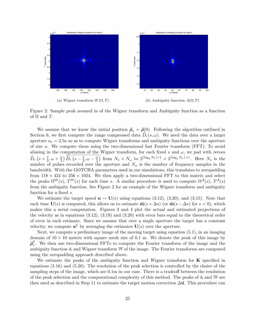
Figure 2: Sample peak zoomed in of the Wigner transform and Ambiguity function as a functionof Ω and T .
We assume that we know the initial position ~ρ? = ~ρ(0). Following the algorithm outlined inSection 6, we first compute the range compressed data Dr(s, ω). We need the data over a largeraperture ae = 2.5a so as to compute Wigner transforms and ambiguity functions over the apertureof size a. We compute them using the two-dimensional fast Fourier transform (FFT). To avoidaliasing in the computation of the Wigner transform, for each fixed s and ω, we pad with zeroes
Dr
(s+ s
2 , ω + ω2
)Dr
(s− s
2 , ω −ω2
)from Ns × Nω to 2dlog2Nse+1 × 2dlog2Nωe+1. Here Ns is the
number of pulses recorded over the aperture and Nω is the number of frequency samples in thebandwidth. With the GOTCHA parameters used in our simulations, this translates to zeropaddingfrom 118 × 424 to 256 × 1024. We then apply a two-dimensional FFT to this matrix and selectthe peaks ΩW(s), TW(s) for each time s. A similar procedure is used to compute ΩA(s), TA(s)from the ambiguity function. See Figure 2 for an example of the Wigner transform and ambiguityfunction for a fixed s.
We estimate the target speed u U(s) using equations (3.12), (3.20), and (3.15). Note thateach time U(s) is computed, this allows us to estimate ~m(s+ ∆s) (or ~m(s−∆s) for s < 0), whichmakes this a serial computation. Figures 3 and 4 plot the actual and estimated projections ofthe velocity as in equations (3.12), (3.19) and (3.20) with error bars equal to the theoretical orderof error in each estimate. Since we assume that over a single aperture the target has a constantvelocity, we compute uI by averaging the estimates U(s) over the aperture.
Next, we compute a preliminary image of the moving target using equation (5.1), in an imagingdomain of 10 × 10 meters with square mesh size of 0.1 m. We denote the peak of this image by~ρI? . We then use two-dimensional FFTs to compute the Fourier transform of the image and theambiguity function A and Wigner transform W of the image. The Fourier transforms are computedusing the zeropadding approach described above.
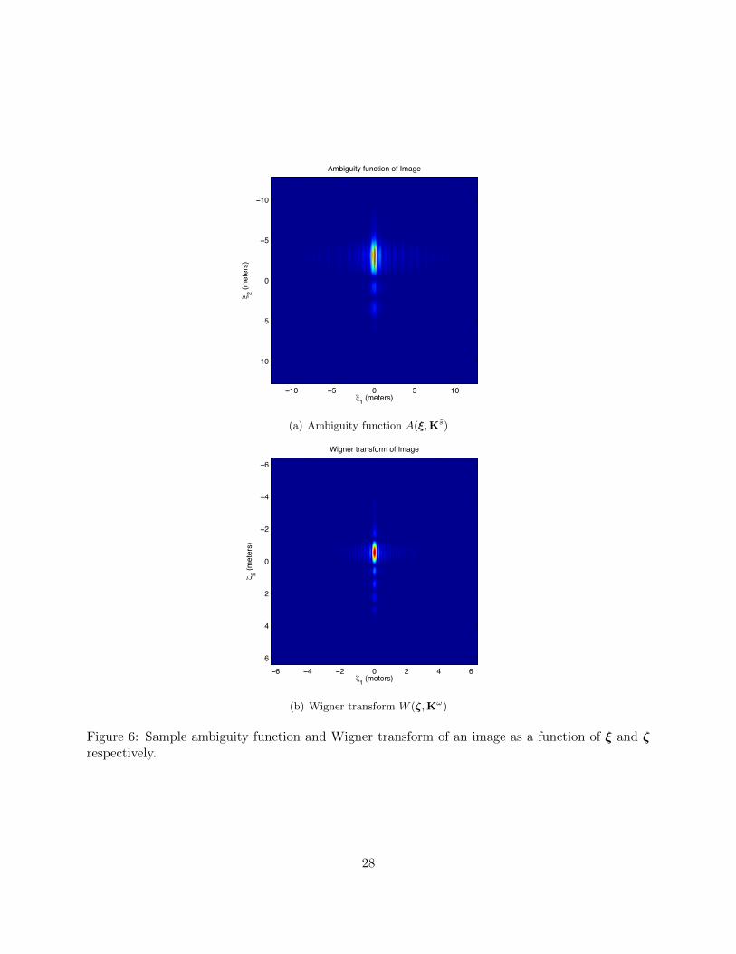
We estimate the peaks of the ambiguity function and Wigner transform for K specified inequations (5.16) and (5.20). The resolution of the peak selection is controlled by the choice of thesampling steps of the image, which are 0.1m in our case. There is a tradeoff between the resolutionof the peak selection and the computational complexity of this method. The peaks of A and W arethen used as described in Step 11 to estimate the target motion correction ∆~u. This procedure can
25

!0.8 !0.6 !0.4 !0.2 0 0.2 0.4 0.6 0.8 1
!0.202
!0.2
!0.198
!0.196
!0.194
!0.192
!0.19
Slow Time (seconds)
Rel
ativ
e Pr
ojec
ted
Velo
city
Relative Velocity Projected on m(s)
Wigner EstimateAmbiguity EstimateActualWigner ResolutionAmbiguity Resolution
Figure 3: Estimated velocity projected onto ~m(s). Estimates were computed using both Wignertransform and ambiguity function. Error bars based on theoretical resolution limits.
!1 !0.8 !0.6 !0.4 !0.2 0 0.2 0.4 0.6 0.8 11.65
1.66
1.67
1.68
1.69
1.7
1.71
1.72
1.73
Slow Time (seconds)
Squa
red
Nor
m o
f Alte
rnat
e R
elat
ive
Proj
ecte
d Ve
loci
ty
Squared Norm of Alternate Relative Projected Velocity
Ambiguity EstimateActualAmbiguity Resolution
Figure 4: Estimated projected velocity in the direction orthogonal to ~m(s). Estimate was obtainedusing the ambiguity function. Error bars based on theoretical resolution limits.
26

!1 !0.8 !0.6 !0.4 !0.2 0 0.2 0.4 0.6 0.8 1
6.782
6.784
6.786
6.788
6.79
6.792
6.794
6.796
6.798
6.8x 10!5
Slow Time (seconds)
Trav
el T
ime
(sec
onds
)
Wigner EstimateActualWigner Resolution
Figure 5: Estimated and actual travel time. Estimate was obtained using the Wigner transform.Error bars based on theoretical resolution limits.
be iterated if necessary. We find that after the first iteration the pair (~ρI? , ~uI) oscillates between
two nearly equal values. This oscillation can be attributed to the discrete sampling of the imagesand the resulting sampling error in selecting the peaks from the ambiguity function and Wignertransform. The results are plotted below in Figures 7 and 8.
7.2 Platform perturbations (autofocus) without target motion
In this section we assume that we have a stationary target at a known location ~ρ? and consider theSAR platform trajectory perturbations of the form:
~µ(s) =
(5λ0s+
λ0
2
s2
2+λ0
20
s3
6, 30λ0, 2λ0s−
λ0
2
s2
2+λ0
20
s3
6
).
Since the target is assumed stationary, we do not use the velocity estimation from the data and beginby computing the image around the target location ~ρ?. Since the resulting image is not centeredaround ~ρ?, we recompute the image in a domain centered around its peak ~ρI? . It is important forthe computation of the ambiguity function and Wigner transform to choose an imaging windowthat contains the peak ~ρI? and a sufficient amount of the sidelobes.
As in the previous section we then compute the ambiguity function A and Wigner transformW for particular values of K. The peaks of A and W are then used to estimate ~µm(s) as describedin Step 11. Finally, the image is recomputed using ~rp(s) + ~µm(s) in place of ~rp(s), as in Step 12.This process can be iterated by updating ~µm(s) until the image converges. The resulting imagesand resolution improvements are plotted in Figures 9 and 10.
27
!1 (meters)
! 2 (met
ers)
Ambiguity function of Image
!10 !5 0 5 10
!10
!5
0
5
10
(a) Ambiguity function A(ξ,Ks)
!1 (meters)
! 2 (met
ers)
Wigner transform of Image
!6 !4 !2 0 2 4 6
!6
!4
!2
0
2
4
6
(b) Wigner transform W (ζ,Kω)
Figure 6: Sample ambiguity function and Wigner transform of an image as a function of ξ and ζrespectively.
28

Cross!Range +meters.
Ran
ge +m
eter
s.
Image with Perfect Motion Estimation
!4 !2 0 2 4
!5
!4
!3
!2
!1
0
1
2
3
4
(a) Image with exact motion estimation
Cross!Range +meters.
Ran
ge +m
eter
s.
Image with Motion Estimation from Data
!4 !2 0 2 4
!5
!4
!3
!2
!1
0
1
2
3
4
(b) Image with motion estimation from data
Cross!Range +meters.
Ran
ge +m
eter
s.
Corrected Image from Image Iteration 2
!4 !2 0 2 4
!5
!4
!3
!2
!1
0
1
2
3
4
(c) Image with motion estimation from both dataand image
Figure 7: Top left: Image with exact target motion. Top right: image with target motion estimatedfrom the data alone. Bottom: Improved image using both the motion estimation from the dataand the correction from the image. The image converges to a peak with ∆x = 0.1 m error in twoiterations.
29

!1 !0.8 !0.6 !0.4 !0.2 0 0.2 0.4 0.6 0.8 10
0.002
0.004
0.006
0.008
0.01
0.012
0.014
0.016
0.018
0.02
Slow Time (seconds)
Dis
tanc
e fro
m T
rue
Traj
ecto
ry (m
eter
s)
Pointwise Error in Motion Estimation
Data Estimated PathImage Estimated Path (Iter 1)Image Estimated Path (Iter 2)Image Estimated Path (Iter 3)Image Estimated Path (Iter 4)Image Estimated Path (Iter 5)
Figure 8: Error in meters between the true trajectory of the moving target and the trajectoryestimated from the data and from the images at several iterations. The algorithm effectivelyconverges in one iteration and has a small oscillation afterwards.
Cross!Range (meters)
Ran
ge (m
eter
s)
Image with Platform Perturbation
!14 !12 !10 !8 !6
!5
!4
!3
!2
!1
0
1
2
3
4
5
(a) Unfocused Image
Cross!Range (meters)
Ran
ge (m
eter
s)
Corrected Image from Image Iteration 2
!5 0 5
!5
!4
!3
!2
!1
0
1
2
3
4
5
(b) Autofocused Image
Figure 9: Images of stationary target with platform perturbation before and after autofocus. Theimage windows are the same size but the left one is translated to a center at the peak of theunfocused image. The image on the right is the autofocused image after two iterations. It focusesat the true target location and the sidelobes are reduced.
8 Summary and conclusions
We have introduced and analyzed in detail from first principles a synthetic aperture radar (SAR)imaging and target motion estimation approach that is combined with compensation for radar plat-form trajectory perturbations. We have formulated an algorithm, in Section 6, that implementsthe theory for a single target and a single small aperture. This algorithm can deal with eithertarget motion estimation or with SAR platform trajectory perturbation, but not with both. Com-bined estimation requires multi-target scenes and multiple, overlapping apertures where the basic
30

!5 !4 !3 !2 !1 0 1 2 3 4 5
!35
!30
!25
!20
!15
!10
!5
0
Cross!Range (meters)
Imag
e In
tens
ity (d
B)
Cross!Range Resolution
No PerturbationPerturbationAutofocused
(a) Cross-range resolution
!5 !4 !3 !2 !1 0 1 2 3 4 5!40
!35
!30
!25
!20
!15
!10
!5
0
Range (meters)
Imag
e In
tens
ity (d
B)
Range Resolution
No PerturbationPerturbationAutofocused
(b) Range Resolution
Figure 10: Cross-range and range resolution of image cross-sections before and after autofocus.Note that the platform perturbations affect basically only the cross-range focus. Note also how theautofocus improves the cross-range resolution and gives an image that is essentially identical to theideal one, without any platform perturbations.
algorithm presented here is used as a component in a broader estimation and imaging strategy.In addition to providing detailed analytical error estimates for the approximations that we use,we verify that they are appropriate for the regime that arises in the GOTCHA Volumetric SARdata set. We also assess the performance of the algorithm of Section 6 with detailed numericalsimulations, presented in Section 7.
Acknowledgement
The work of L. Borcea was partially supported by the National Science Foundation, grants DMS-0604008, DMS-0934594, DMS-0907746, by the Office of Naval Research grants N000140910290and N000140510699, and by Air Force - SBIR FA8650-09-M-1523. The work of T. Callaghan waspartially supported by AFOSR grant FA9550-08-1-0089. The work of G. Papanicolaou was partiallysupported by AFOSR grant FA9550-08-1-0089 and by Air Force - SBIR FA8650-09-M-1523. Wethank Elizabeth Bleszynski, Marek Bleszynski and Thomas Jaroszewicz of Monopole Research withwhom we collaborated in the Air Force SBIR.
Appendices
A The probing signal
The base-band signals fB(t) in (2.3) may be short pulses, of width O(1/B), that give images withrange resolution ∼ c/B. However, such pulses are rarely used in SAR because they have low signalto noise ratio (SNR) [7]. Chirped waveforms of the form
f(t) = e−iωot+iσt2χ
(t
tc
)(A.1)
31

are preferred in SAR because for a given bandwidth B that gives good range resolution, they havea long waveform, that is, tc 1/B, and therefore higher SNR. The signal (A.1) is a linear fre-quency modulated chirp, with frequency modulation parameter σ > 0 and support in [−tc/2, tc/2],determined by pulse shape function χ (·/tc). In the frequency domain it has the form
f(ω) = fB(ω − ωo) =
∫ ∞−∞
dt χ
(t
tc
)ei(ω−ωo)t+iσt
2
= e−i(ω−ωo)2
4σ
∫ ∞−∞
dw
2πχ(w)ei
w(ω−ωo)2σtc
∫ ∞−∞
dt eiσ(t+ω−ωo2σ )
2−i wtc
(t+ω−ωo2σ )
=
√iπ
σe−
i(ω−ωo)24σ
∫ ∞−∞
dw
2πχ(w)e
iw(ω−ωo)
2σtc−i w
2
4σt2c .
Assuming that tc 1/√σ, this simplifies to
f(ω) = fB(ω − ωo) ≈√iπ
σe−
i(ω−ωo)24σ χ
(ωo − ω2σtc
). (A.2)
Thus, f(ω) is supported in the frequency interval
|ν − νo| =|ω − ωo|
2π≤ σtc
2π=B
2,
of length σtc/π = B, with B the chirp bandwidth. The assumption tc 1/√σ implies that for
given bandwidth B the width in time tc of the chirp is much longer than 1/B, tc 1/B. In atypical SAR setup tc is constrained by
tc =πB
σ< ∆s,
so that the support of the probing signal does not exceed the signal repetition rate ∆s. Since,∣∣∣f(ω)∣∣∣ =
∣∣∣fB(ω − ωo)∣∣∣ ≈√π
σ
∣∣∣∣χ(ω − ωo2σtc
)∣∣∣∣ , (A.3)
then in the case χ(t/tc) = 1[−tc/2,tc/2](t) we can make the approximation∣∣∣f(ω)∣∣∣ ≈ ∣∣∣fB(0)
∣∣∣ for all ω ∈ [ωo − σtc, ωo + σtc] . (A.4)
B Proof of Proposition 1
We begin with equation (2.2), where we make the change of variables
x = ρζ(s) + ut′, ρζ(s) = ρ(s) + ζ,
and approximate
~rp(s+ t) ≈ ~rp(s) + ~V(s)t, ~V(s) =∂~rp(s+ t)
∂t
∣∣∣∣t=0
. (B.1)
32

We get
D(s, t) ≈ ω2o
c2
∫dζ gc(ζ)
∫dt′
δ(t− t′ − |~rp(s) + ~V(s)t− ~ρζ(s)− ~ut′|/c)4π|~rp(s) + ~V(s)t− ~ρζ(s)− ~ut′|
f(t′ − |~rp(s)− ~ρζ(s)− ~ut′|/c)4π|~rp(s)− ~ρζ(s)− ~ut′|
, (B.2)
in narrow-band regimes πB ωo, where
∂2t f(t) ≈ −ω2
of(t) = −ω2oe−iωotfB(t).
The data model follows from (B.2) and the approximations
|~rp(s) + ~V(s)t− ~ρζ(s)− ~ut′| ≈ |~rp(s)− ~ρζ(s)|+ (~V(s)t− ~ut′) · ~mζ(s),
|~rp(s)− ~ρζ(s)− ~ut′| ≈ |~rp(s)− ~ρζ(s)| − ~ut′ · ~mζ(s),
with negligible error O(|~V(s)t|2/|~rp(s)− ~ρζ(s)|
)over the small time interval t ∈ (0,∆s). Here we
introduce the unit vector
~mζ(s) =~rp(s)− ~ρζ(s)
|~rp(s)− ~ρζ(s)|.
We obtain that
t′[1−
~u
c· ~mζ(s)
]≈ t
[1−
~V(s)
c· ~mζ(s)
]−|~rp(s)− ~ρζ(s)|
c
and therefore
D(s, t) ≈ ω2o
c2
∫dζ
gc(ζ)
(4π|~rp(s)− ~ρζ(s)|)2f
t
[1 +
(2~u
c−~V(s)
c
)· ~mζ(s) +O
(|~V(s)|2
c2
)]−
2|~rp(s)− ~ρζ(s)|c
[1 +
~u
c· ~mζ(s) +O
(|~u(s)|2
c2
)]. (B.3)
Neglecting the quadratic terms
|~u(s)|2
c2.|~V(s)|2
c2 1,
and Fourier transforming in t, we get
D(s, ω) ≈ ω2o
c2
∫dζ
gc(ζ)
(4π|~rp(s)− ~ρζ(s)|)2fB
ω
1 +(
2~uc −~V(s)c
)· ~mζ(s)
− ωo
exp
iω
2|~rp(s)− ~ρζ(s)|c
[1 +
(~V(s)
c−~u
c
)· ~mζ(s)
]. (B.4)
Since the support of fB is of order πB, we can write
fB(·) = F( ·πB
),
33

with F supported in [−1, 1] and approximate
fB
ω
1 +(
2~uc −~Vc
)· ~mζ(s)
− ωo
≈ F (ω − ωoπB
− ω
πB
(2~u
c−~V
c
)· ~mζ(s)
)≈ fB(ω − ωo),
because by (2.7),
ω
πB
|2~u− ~V(s)|c
∼ νoB
|~V(s)|c 1.
The mathematical model of the data is
D(s, ω) ≈ ω2o
c2
∫dζ
gc(ζ)
(4π|~rp(s)− ~ρζ(s)|)2fB(ω − ωo) exp
[iω τ(s, ~ρζ(s)) + iωψζ(s)
],
and if we assume further that the central frequency is high enough for equation
ωψζ(s) =2ωoc
(~V(s)
c−~u
c
)·(~rp(s)− ~ρζ(s)
)∼ 1 (B.5)
to hold (recall (2.6)), we obtain using the narrow band condition πB ωo and |ζ| |~rp(s)−~ρ(s)|that
ωψζ(s) ≈ ωoψ(s), (B.6)
with
ψ(s) =2
c
(~V(s)
c−~u
c
)· (~rp(s)− ~ρ(s)) . (B.7)
Therefore
D(s, ω) ≈ ω2o fB(ω − ωo)eiωoψ(s)
c2
∫dζ
gc(ζ)
(4π|~rp(s)− ~ρζ(s)|)2exp eiω τ(s,~ρζ(s)). (B.8)
This concludes the proof of Proposition 1.Equation (2.12) follows directly from equations (B.3) and (B.4), with the exception that we
cannot replace ∂2t f(t) by −ω2
of(t) anymore, so we should use in (B.4) −ω2fB(ω − ωo), the Fouriertransform of ∂2
t f(t).Finally, equation (2.13) is essentially equation (B.4), where we get the detectable Doppler
frequency shift by the factor(~V(s)c −
2~uc
)· ~m(s), in the very narrow band case satisfying ωo
πB|~V(s)|c ∼
1.
C Proof of Proposition 2
For a small enough time offset bound S we can approximate the amplitudes of Dr
(s± s
2 , ω ±ω2
)1(
4π|~rp(s± s
2
)− ~ρ
(s± s
2
)|)2 ≈ 1
(4π|~rp(s)− ~ρ(s)|)2
34

and obtain
W(s,Ω, ωo, T ) ∼ |fB(0)|4
|~rp(s)− ~ρ(s)|4
∫ 2πB
−2πBdω
∫ S
−Sds eiΦ
W (ω,s,s,ωo),
with phase given by
ΦW(ω, s, s, ωo) =2ωocT1(s, s) +
ω
cT2(s, s) + sΩ− ωT. (C.1)
Here we let
T1(s, s) =
∣∣∣∣~rp(s+s
2
)− ~ρ
(s+
s
2
)∣∣∣∣− ∣∣∣∣~rp(s− s
2
)− ~ρ
(s− s
2
)∣∣∣∣−∣∣∣∣~rp(s+s
2
)− ~ρo
∣∣∣∣+
∣∣∣∣~rp(s− s
2
)− ~ρo
∣∣∣∣ , (C.2)
and
T2(s, s) =
∣∣∣∣~rp(s+s
2
)− ~ρ
(s+
s
2
)∣∣∣∣+
∣∣∣∣~rp(s− s
2
)− ~ρ
(s− s
2
)∣∣∣∣−∣∣∣∣~rp(s+s
2
)− ~ρo
∣∣∣∣− ∣∣∣∣~rp(s− s
2
)− ~ρo
∣∣∣∣ . (C.3)
Now let us note that∣∣∣∣~rp(s+s
2
)− ~ρ
(s+
s
2
)∣∣∣∣− ∣∣∣∣~rp(s− s
2
)− ~ρ
(s− s
2
)∣∣∣∣ = s(~V(s)− ~u
)· ~m(s) +
O
(s3
24
d3 |~rp(s)− ~ρ(s)|ds3
), (C.4)
becaused |~rp(s)− ~ρ(s)|
ds=(~V(s)− ~u
)· ~m(s), (C.5)
and~V(s) = ~r′p(s) = V (s)~t(s), ~u = ~ρ′(s). (C.6)
Recall from (3.2) that ~t(s) is the unit vector tangential to the platform trajectory, and from (2.10)that ~m(s) is the unit vector
~m(s) =~rp(s)− ~ρ(s)
|~rp(s)− ~ρ(s)|. (C.7)
Assuming that both the target speed ~u, and the tangential platform speed V (s) change slowly ins, we drop their s dependence and approximate the second derivative of |~rp(s)− ~ρ(s)| by
d2 |~rp(s)− ~ρ(s)|ds2
≈ V~t′(s) · ~m(s) +(V~t(s)− ~u
)· ~m′(s), (C.8)
and the third derivative by
d3 |~rp(s)− ~ρ(s)|ds3
≈ V~t′′(s) · ~m(s) + 2V~t′(s) · ~m′(s) +(V~t(s)− ~u
)· ~m′′(s). (C.9)
35

We obtain therefore∣∣∣∣~rp(s+s
2
)− ~ρ
(s+
s
2
)∣∣∣∣− ∣∣∣∣~rp(s− s
2
)− ~ρ
(s− s
2
)∣∣∣∣ ≈ s(~V(s)− ~u)· ~m(s) +
s3
24
[V~t′′(s) · ~m(s) + 2V~t′(s) · ~m′(s) +
(V~t(s)− ~u
)· ~m′′(s)
]. (C.10)
A similar calculation gives∣∣∣∣~rp(s+s
2
)− ~ρo
∣∣∣∣− ∣∣∣∣~rp(s− s
2
)− ~ρo
∣∣∣∣ ≈ s ~V(s) · ~mo(s) +s3
24
[Vd2~t(s)
ds2· ~mo(s)+
2Vd~t(s)
ds· d~mo(s)
ds+ V~t(s) · d
2 ~mo(s)
ds2
], (C.11)
where
~mo(s) =~rp(s)− ~ρo|~rp(s)− ~ρo|
.
Thus, we obtain
2ωocT1(s, s) ≈ −2ωos~u
c· ~m(s) +
2ωosV
c~t(s) · ( ~m(s)− ~mo(s)) +
ωos3V 3
12cE1(s), (C.12)
with scaled remainder
V 2E1(s) = −~u
V· ~m′′(s) +~t′′(s) · [ ~m(s)− ~mo(s)] + 2~t′(s) ·
[~m′(s)− ~m′o(s)
]+
~t(s) ·[~m′′(s)− ~m′′o(s)
]. (C.13)
The derivatives of ~t(s) are determined by the differential geometry relations
~t′(s) = −VR~n(s), ~t′′(s) = −V
R~n′(s) = −V
2
R2~t(s), (C.14)
with ~n(s) the unit vector orthogonal to ~t(s), in the flight plane defined by ~t(s) and the center ofcurvature, at distance R from ~rp(s). The derivative of ~m(s) is
~m′(s) =P(s)
(V~t(s)− ~u
)|~rp(s)− ~ρ(s)|
, P(s) = I − ~m(s) ( ~m(s))T , (C.15)
and
~m′′(s) =P(s)V~t′(s) + P′(s)
(V~t(s)− ~u
)|~rp(s)− ~ρ(s)|
−P(s)
(V~t(s)− ~u
)|~rp(s)− ~ρ(s)|2
(V~t(s)− ~u
)· ~m(s) (C.16)
is a vector orthogonal to ~m′(s), with norm ∼ V 2/L2. Similarly, we have
~m′o(s) =V Po(s)~t(s)|~rp(s)− ~ρo|
, where Po(s) = I − ~mo(s) ( ~mo(s))T , (C.17)
36

and
~m′′o(s) =V Po(s)~t′(s) + V P′o(s)~t(s)
|~rp(s)− ~ρo|− V Po(s)~t(s)|~rp(s)− ~ρo|2
V~t(s) · ~mo(s). (C.18)
Now, assuming a reference point ~ρo that is close enough to ~ρ
|~ρ(s)− ~ρo| |~rp(s)− ~ρo| ∼ L, (C.19)
we can write
~m(s) = ~mo(s)−Po(s) (~ρ(s)− ~ρo)|~rp(s)− ~ρo|
+ ~E , |~E| = O
(|~ρ(s)− ~ρo|2
L2
), (C.20)
and ∣∣ ~m′(s)− ~m′o(s)∣∣ = O
(|~u|L
),∣∣ ~m′′(s)− ~m′′o(s)
∣∣ = O
(V |~u|L2
). (C.21)
Thus, equations (C.12), (C.13) and (C.19) give
2ωocT1(s, s) = −2ωos~u
c· ~m(s) +
2ωosV
c~t(s) · ( ~m(s)− ~mo(s)) +
ωos3V 3
12cE1(s),
with negligible remainder E1(s) = O(|~u|V L2
), when we chose the aperture SV = a/2 so that
(a/2)3 λoL2V/|~u|. (C.22)
This is the second assumption in (3.6).To approximate T2(s, s), we use (C.8) and (C.14) to get∣∣∣∣~rp(s+
s
2
)− ~ρ
(s+
s
2
)∣∣∣∣+
∣∣∣∣~rp(s− s
2
)− ~ρ
(s− s
2
)∣∣∣∣ = 2 |~rp(s)− ~ρ(s)|+
s2
8
[V~t′(s) · ~m(s) +
(V~t(s)− ~u
)· ~m′(s)
]+O
(s4
4!
d4|~rp(s)− ~ρ(s)|ds4
), (C.23)
and similarly,∣∣∣∣~rp(s+s
2
)− ~ρo
∣∣∣∣+
∣∣∣∣~rp(s− s
2
)− ~ρo
∣∣∣∣ = 2 |~rp(s)− ~ρo|+s2
8Vd~t(s)
ds· ~mo(s) +
s2
8V~t(s) · d
~mo(s)
ds+O
(s4
4!
d4|~rp(s)− ~ρ(s)|ds4
)(C.24)
Thus, we can write
ω
cT2(s, s) =
2ω
c(|~rp(s)− ~ρ(s)| − |~rp(s)− ~ρo|) +
ωs2
8cE2(s, s) (C.25)
with scaled remainder
E2(s, s) = O
(V 2|~ρ(s)− ~ρo|
L2
)+O
(V |~u|L
), (C.26)
37
that can be neglected if(a/2)2
λoL νoV
B|~u|. (C.27)
This is the first assumption in (3.6). Note that the other term in the remainder E2 is small because
ωs2V 2|~ρ(s)− ~ρo|c|~rp(s)− ~ρo|2
∼ B
νo
(a/2)2
λoL
|~ρ(s)− ~ρo|L
V
|~u||~ρ(s)− ~ρo|
L 1.
Gathering all the results we obtain the phase approximation
ΦW(ω, s, s, ωo) ≈ sωo[
Ω
ωo− 2~u
c· ~m(s) +
2V
c~t(s) · ( ~m(s)− ~mo(s))
]+
ω [τ(s, ~ρ(s))− τ(s, ~ρo)− T ] , (C.28)
and Proposition 2 follows after substituting Φ in the expression of the Wigner transformW(s,Ω, ωo, T ),and integrating over s and ω.
When we relax the first assumption in (3.6) to (3.11), the remainder E2 in (C.25) is no longernegligible, and we obtain a Fresnel integral in s. The method of stationary phase [2] tells us thatthe quadratic term in (C.25) does not affect the location of the peak of this integral, which is theinformation used in the target motion estimation.
D Proof of Proposition 3
We have from the definition (3.17) and Appendix C that
A(s,Ω, a/(2V ), T ) ∼ |fB(0)|4
|~rp(s)− ~ρ(s)|4
∫dω
∫ S
−Sds eiΦ
A(s,s,ω), (D.1)
with phase ΦA given by a minor modification of (C.28), with ω set to zero,
ΦA(s, s, ω) ≈ aω
c
[~t(s+ s) · ( ~m(s+ s)− ~mo(s+ s))−
~u
V· ~m(s+ s)
]+ sΩ− ωT. (D.2)
Now use equations (C.5)-(C.15) to write(~t(s+ s)−
~u
V
)· ~m(s+ s) =
(~t(s)−
~u
V
)· ~m(s) + s
[~t′(s) · ~m(s) +
(~t(s)−
~u
V
)· ~m′(s)
]+O
(a2
L2
)and
~t(s+ s) · ~mo(s+ s) = ~t(s) · ~mo(s) + s[~t′(s) · ~mo(s) +~t(s) · ~m′o(s)
]+O
(a2
L2
).
Using (C.15) and (C.17), we get
(~t(s)−
~u
V
)· ~m′(s) =
(~t(s)−
~u
V
)·P(s)
(~V(s)− ~u
)|~rp(s)− ~ρ(s)|
=V∣∣∣P(s)
(~t(s)− ~u
V
)∣∣∣2|~rp(s)− ~ρ(s)|
38
and
~t(s) · ~m′o(s) = ~t(s) · Po(s)~V(s)
|~rp(s)− ~ρo|=V∣∣∣Po(s)~t(s)∣∣∣2|~rp(s)− ~ρo|
.
We shall keep only the leading order terms, as the error is ∼ a3/λoE1(s), with E1(s) given by(C.13), and it becomes negligible when (a/2)3 λoL
2V/ |~u|. The phase (D.2) becomes
ΦA(s, s, ω) ≈ s
aV ωoc
[~t′(s)
V· ( ~m(s)− ~mo(s)) +
∣∣∣P(s)(~t(s)− ~u
V
)∣∣∣2|~rp(s)− ~ρ(s)|
−
∣∣∣Po(s)~t(s)∣∣∣2|~rp(s)− ~ρo|
+ Ω
+
ω
a
c
[~t(s) · ( ~m(s)− ~mo(s))−
~u
V· ~m(s)
]− T
+ E3,
with ~t′(s) given by (C.14), and remainder
E3 =asV (ω − ωo)
c
~t′(s)V· ( ~m(s)− ~mo(s)) +
∣∣∣P(s)(~t(s)− ~u
V
)∣∣∣2|~rp(s)− ~ρ(s)|
−
∣∣∣Po(s)~t(s)∣∣∣2|~rp(s)− ~ρo|
=
Ba2
cLO
(|~u|V
+|~rp(s)− ~ρo|
L
)= O
(Ba2|~u|νoλoLV
)(D.3)
that can be neglected under the first assumption in (3.6). We obtain
ΦA(s, s, ω) ≈ saV ωoc
[~t′(s) · ( ~m(s)− ~mo(s))
V+
∣∣∣P(s)(~t(s)− ~u
V
)∣∣∣2|~rp(s)− ~ρ(s)|
−
∣∣∣Po(s)~t(s)∣∣∣2|~rp(s)− ~ρo|
+ Ω
+
ω
a
c
[~t(s) · ( ~m(s)− ~mo(s))−
~u
V· ~m(s)
]− T
,
and Proposition 3 follows after substituting ΦA in (D.1) and integrating in ω and s.Finally, when we relax the first assumption in (3.6) to (3.11), we obtain
ΦA(s, s, ω) ≈ s
aV ωc~t′(s) · ( ~m(s)− ~mo(s))
V+
∣∣∣P(s)(~t(s)− ~u
V
)∣∣∣2|~rp(s)− ~ρ(s)|
−
∣∣∣Po(s)~t(s)∣∣∣2|~rp(s)− ~ρo|
+ Ω
+
ω
a
c
[~t(s) · ( ~m(s)− ~mo(s))−
~u
V· ~m(s)
]− T
,
and the ambiguity function A(s,Ω, a/(2V ), T ) cannot be written explicitly, due to the coupling ofthe integrals over ω and s. Nevertheless, we can infer from the method of stationary phase [2] thatthe coupling does not affect the location of the peaks of A(s,Ω, a/(2V ), T ), which is what we needin the motion estimation.
39

E Proof of Theorems 1 and 2.
The perturbation of the phase (C.1) of the Wigner transform of the range compressed data (4.1)is given by
δΦW(ω, s, s, ωo) =2ωocδT1(s, s) +
ω
cδT2(s, s), (E.1)
where
δT1(s, s) =
∣∣∣∣~rp(s+s
2
)+ ~µ
(s+
s
2
)− ~ρ
(s+
s
2
)∣∣∣∣− ∣∣∣∣~rp(s− s
2
)+ ~µ
(s− s
2
)− ~ρ
(s− s
2
)∣∣∣∣−∣∣∣∣~rp(s+
s
2
)− ~ρ
(s+
s
2
)∣∣∣∣+
∣∣∣∣~rp(s− s
2
)− ~ρ
(s− s
2
)∣∣∣∣ , (E.2)
and
δT2(s, s) =
∣∣∣∣~rp(s+s
2
)+ ~µ
(s+
s
2
)− ~ρ
(s+
s
2
)∣∣∣∣+
∣∣∣∣~rp(s− s
2
)+ ~µ
(s− s
2
)− ~ρ
(s− s
2
)∣∣∣∣−∣∣∣∣~rp(s+
s
2
)− ~ρ
(s+
s
2
)∣∣∣∣− ∣∣∣∣~rp(s− s
2
)− ~ρ
(s− s
2
)∣∣∣∣ . (E.3)
Proceeding as in Appendix C, we write
δT1(s, s) = s(V~t(s) + ~µ′(s)− ~u
)· ~mµ(s)− s
(V~t(s)− ~u
)· ~m(s) +
O
(s3
24
∣∣∣∣d3 [~rp(s) + ~µ(s)− ~ρ(s)|ds3
− d3 |~rp(s)− ~ρ(s)|ds3
]),
using the identity
d|~rp(s) + ~µ(s)− ~ρ(s)|ds
=(V~t(s) + ~µ′(s)− ~u
)· ~mµ(s), (E.4)
and
~mµ(s) =~rp(s) + ~µ(s)− ~ρ(s)
|~rp(s) + ~µ(s)− ~ρ(s)|= ~m(s) +
P(s)~µ(s)
|~rp(s)− ~ρ(s)|+ ~E , |~E| = O
(|~µ(s)|2
|~rp(s)− ~ρ?|2
). (E.5)
Then, we have
d2 |~rp(s) + ~µ(s)− ~ρ(s)|ds2
=(V~t′(s) + ~µ′′(s)
)· ~mµ(s) +
(V~t(s) + ~µ′(s)− ~u
)· ~m′µ(s), (E.6)
where
~m′µ(s) =Pµ(V~t(s) + ~µ′(s)− ~u
)|~rp(s) + ~µ(s)− ~ρ(s)|
, Pµ(s) = I − ~mµ(s) ( ~mµ(s))T , (E.7)
and furthermore,
d3 |~rp(s) + ~µ(s)− ~ρ(s)|ds3
≈(V~t′′(s) + ~µ′′′(s)
)· ~mµ(s) + 2
(V~t′(s) + ~µ′′(s)
)· ~m′µ(s) +(
V~t(s) + ~µ′(s)− ~u)· ~m′′µ(s). (E.8)
40

The second derivative of ~mµ(s) is given by
~m′′µ(s) =Pµ(V~t′(s) + ~µ′′(s)
)+ P′µ(s)
(V~t(s) + ~µ′(s)− ~u
)|~rp(s) + ~µ(s)− ~ρ(s)|
−
Pµ(s)(V~t(s) + ~µ′(s)− ~u
)|~rp(s) + ~µ(s)− ~ρ(s)|2
(V~t(s) + ~µ′(s)− ~u
)· ~mµ(s). (E.9)
and its magnitude is of order∣∣∣∣d2 ~mµ(s)
ds2
∣∣∣∣ = O
(V 2
L2
)+O
(∣∣~µ′′(s)∣∣L
), (E.10)
because |~µ′(s)| V . Thus, we obtain
2ωos
cδT1(s, s) =
2ωos
c~µ′(s) · ~m(s) +
2ωosV
c
(~t(s)−
~u
V
)· P~µ(s)
|~rp(s)− ~ρ(s)|+ωoV s
cE4(s), (E.11)
with scaled remainder
ωoV s
cE4(s) = O
(ωoc
a~µ′(s)
V· P(s)~µ(s)
L
)+O
(a|~µ(s)|2
λoL2+
a3
λoL2+
a
λoL
a2|~µ′′(s)|V 2
+a3|~µ′′′ · ~mµ(s)|
V 3λo
).
The first term in the remainder is negligible by (4.6),
ωoc
a
V~µ′(s) · P(s)~µ(s)
L∼ 1
λo
λoL
aδ
µ
L=
µ
aδ 1.
The second term is negligible because
a|~µ(s)|2
λoL2∼ µ2
a2
a3
λoL2 1,
by (3.6) and |~u| . V , and the fourth term is negligible by assumption (4.8)
a2|~µ′′(s)|V 2
∼ λoγ,
for all γ a/L, not only γ ∼ δ, as assumed in in (4.15). Finally, the last term in the remainder isnegligible by assumption (4.9).
We have now shown that
2ωos
cδT1(s, s) ≈ 2ωos
c~µ′(s) · ~m(s) +
2ωosV
c
(~t(s)−
~u
V
)· P(s)~µ(s)
|~rp(s)− ~ρ(s)|. (E.12)
Similarly, we getω
cδT2(s, s) =
2ω
c~µ(s) · ~m(s) + E5(s, s)
with remainder
E5(s, s) = O
(ω
c
µ2
L
)+O
(ω
c
a2
V 2
[d2|~rp(s) + ~µ(s)− ~ρ(s)|
ds2− d2|~rp(s)− ~ρ(s)|
ds2
]).
41

The first term in this remainder is negligible by (3.6) and the assumption |~µ| ∼ µ a. Note from(E.6) that the second term in E5 is similar to the remainder E2 estimated in Appendix C, and thatall terms but
ω
c
a2
V 2~µ′′(s) · ~mµ(s) ∼ B
νoγ
are negligible under our assumptions.Therefore, we get
ω
cδT2(s, s) ≈ 2ω
c~µ(s) · ~m(s) +
ω
c
s2
2~µ′′(s) · ~mµ(s) (E.13)
and the perturbation of the phase in the Wigner transform is given by
δΦW(ω, s, s, ωo) ≈2ωosV
c
[1
V~µ′(s) · ~m(s) +
(~t(s)−
~u
V
)· P(s)~µ(s)
|~rp(s)− ~ρ(s)|
]+
2ω
c~µ(s) · ~m(s) +
ω
c
s2
2~µ′′(s) · ~mµ(s). (E.14)
The last term in δΦW(ω, s, s, ωo) is of order B/(νoγ), and can be neglected when γ ∼ δ B/νo.Theorem 1 follows from (E.14) and (C.28), after integration in s and ω.
When γ . B/νo, we obtain a more complicated expression of W, involving a Fresnel integral in
s. However, the quadratic phase ωcs2
2 ~µ′′(s) · ~mµ(s) does not affect the location of the peak of the
resulting integral in s [1], which means that the velocity estimation described in Section 4.2 shouldwork for γ . B/νo, as well.
The perturbation of the phase (D.2) of the ambiguity function is given by
δΦA(s, s, ω) ≈ aω
c
[1
V~µ′(s+ s) · ~mµ(s+ s) +
(~t(s+ s)−
~u
V
)· ( ~mµ(s+ s)− ~m(s+ s))
].
Expanding in s we get
δΦA(s, s, ω) ≈ aω
c
[~µ′(s)
V· ~m(s) +
(~t(s)−
~u
V
)· P(s)~µ(s)
|~rp(s)− ~ρ(s)|
]+
asV ω
c
~µ′′(s)V 2
· ~m(s) + 2P(s)
(~t(s)−
~u
V
)·
P(s)~µ′(s)V
|~rp(s)− ~ρ(s)|+
∣∣∣P(s)~µ′(s)V
∣∣∣2|~rp(s)− ~ρ(s)|
+ E6,
with negligible remainder E6, as in Appendix D and the estimation of E5.
F Proof of Proposition 4.
Let us begin with the model (4.1) of the range compressed data, which we simplify by approximatingthe geometrical spreading factors (amplitudes) by a constant. The imaging function is given by
I(ρI) ∼∫ S
−Sds
∫ ωo+πB
ωo−πBdω e
2iωc (|~rp(s)+~µ(s)−~ρ?−s~u|−|~rp(s)−~ρ I−s~uI |), (F.1)
42

where ~uI satisfies (4.15), and the smooth part ~µ(s) of the platform trajectory perturbation satisfiesthe scaling assumptions (4.4)-(4.12). It is convenient for the analysis in the next sections to expandthe phase in I(ρI) around the peak ρI? of the image, which is yet to be determined. That is, wewrite
ρI = ρI? + ζI . (F.2)
Now, let us denote by
Φ(s) = |~rp(s) + ~µ(s)− ~ρ? − s~u| − |~rp(s)− ~ρ I − s~uI | (F.3)
the phase in (F.1) and expand it in s
Φ(s) = Φ(0) + sΦ′(0) +s2
2Φ′′(0) +O
(s3
3!Φ′′′(s)
). (F.4)
The remainder O(s3
3! Φ′′′(s)
)is negligible, as proved in Appendix E, and
Φ(0) = |~rp − ~ρ? + ~µ| − |~rp − ~ρI? − ~ζI|,
Φ′(0) = (V~t− ~u + ~µ′) · ~mµ − (V~t− ~uI) · ~MI , (F.5)
Φ′′(0) = (V~t′ + ~µ′′) · ~mµ + (V~t− ~u + ~µ′) · ~m′µ − V~t′ · ~MI − (V~t− ~uI) · ~M′I ,
where
~mµ(s) =~rp(s) + ~µ(s)− ~ρ? − s~u|~rp(s) + ~µ(s)− ~ρ? − s~u|
and
~MI (s) =~rp(s)− ~ρI? − ~ζ
I− s~uI
|~rp(s)− ~ρI? − ~ζI− s~uI |
.
Note the simplified notation in (F.5), with the convention that when the arguments are missing,we evaluate the function at s = 0, as in ~rp(0) ~rp.
Now, let us approximate each term in (F.4). We have
Φ(0) = |~rp − ~ρ?| − |~rp − ~ρI? |+ ~m? · ~µ + ~mI · ~ζI
+O
(|~ζI|2 + µ2
L
), (F.6)
where
~m? =~rp − ~ρ?|~rp − ~ρ?|
and ~mI =~rp − ~ρI?|~rp − ~ρI? |
, (F.7)
and the remainder is negligible by (4.4) and because
|~ζI| . λoL
a√λoL. (F.8)
To evaluate the next term in (F.4), we use
~mµ = ~m? +P?~µ|~rp − ~ρ?|
+ ~E , |~E| = O
(µ2
L2
)43

and
~MI = ~mI −PI~ζ
I
|~rp − ~ρI? |+ ~E , |~E| = O
(|~ζI|2
L2
),
with P? = I − ~m? ~mT? and PI = I − ~mI ( ~mI )
T , and get
sV Φ′(0) = sV
(~t−
~uI
V
)·
(~m? − ~mI +
P?~µ|~rp − ~ρ?|
+PI~ζ
I
|~rp − ~ρI? |
)+ sV
(∆~u + ~µ′)
V· ~m? +
O
(a
L
(|~ζI|2 + µ2)
L+aµ
L
|∆~u + ~µ′|V
). (F.9)
Here we let ∆~u = ~uI − ~u and we note that the remainder is negligible by assumptions (4.4), (F.8),(4.12) and a L.
For the last term in (F.4) we use that
~m′µV
=
(I − ~mµ ~m
Tµ
) (~t− ~uI
V + ∆~u+~µ′
V
)|~rp + ~µ− ~ρ? − ~ζ|
=P?(~t− ~uI
V + ∆~u+~µ′
V
)|~rp − ~ρ?|
+ ~E , |~E| = O
(µ
L2
),
and
~M′IV
=
(I − ~MI
~MTI
)(~t− ~uI
V
)|~rp + ~µ− ~ρI? − ~ζ
I|
=PI(~t− ~uI
V
)|~rp − ~ρI? |
+ ~E , |~E| = O
(|~ζI|
L2
).
We also have ~t′/V = −~n/R, and obtain
(sV )2Φ′′(0) = (sV )2
~µ′′ · ~m?
V 2−~n
R· ( ~m? − ~mI ) +
∣∣∣P? (~t− ~uI
V + ∆~u+~µ′
V
)∣∣∣2|~rp − ~ρ?|
−
∣∣∣PI (~t− ~uI
V
)∣∣∣2|~rp − ~ρI? |
+
O
(a2(1 + L|~µ′′ · ~m?|/V 2
)µ
L2+a2|~ζ
I|
L2
). (F.10)
SinceL|~µ′′ · ~m?|
V 2∼ Lλoεa2 1
by assumptions (4.8) and (4.12), we note that we can neglect the remainder in (F.10), because
|~ζI| λoL
2
a2and µ λoL
2
a2.
These inequalities follow from (F.8), (3.6) since
√λoL
λoL2/a2=
√a
L
√a3
λoL3√a
L
V
|~u|,
and |~u| . V .
44

We have obtained that
I(ζI) ∼∫ S
−Sds
∫ ωo+πB
ωo−πBdω exp
2iω
c
[|~rp − ~ρ?| − |~rp − ~ρI? |+ ~mI · ~ζ
Iϕo
]+
2iωsV
c
[(~t−
~uI
V
)·
(~m? − ~mI +
PI~ζI
|~rp − ~ρI? |
)+ ϕ1
]+iω(sV )2
cϕ2
, (F.11)
with ϕ0, ϕ1 and ϕ2 given in Proposition 4. Now, let us note that
2ωsV
c
(~t−
~uI
V
)· PI~ζ
I
|~rp − ~ρI? |=
2ωosV
c
(~t−
~uI
V
)· PI~ζ
I
|~rp − ~ρI? |+O
(Ba
c
|~ζI|
L
)and the remainder is negligible because
Ba
c
|~ζI|
L Ba
c
λoa∼ B
νo 1,
by assumption (F.8).We show next that we can also approximate
ω(sV )2
cϕ2 ≈
ωo(sV )2
cϕ2.
Indeed, we have
ω(sV )2
c
∣∣∣P? (∆~u+~µ′
V
)∣∣∣2|~rp − ~ρ?|
=ωo(sV )2
c
∣∣∣P? (∆~u+~µ′
V
)∣∣∣2|~rp − ~ρ?|
+O
a2B
c
∣∣∣∆~u+~µ′
V
∣∣∣2L
with negligible remainder because
a2B
c
∣∣∣∆~u+~µ′
V
∣∣∣2L
∼ B
νoλoL
(λoL
aε
)2
=B
νoε
λoL
a2ε B
νoε Ba2
νoλoL. 1,
by (4.15), (4.12) and (3.6). We also have
ω(sV )2
c
~t′
V· ( ~m? − ~mI ) =
ωo(sV )2
c
~t′
V· ( ~m? − ~mI ) +O
(a2B
cL| ~m? − ~mI |
)with remainder
a2B
cL| ~m? − ~mI | =
Ba2
νoλoL| ~m? − ~mI | .
V
|~u|| ~m? − ~mI | =
V
|~u|
(|~ρ?|+ |~ρI? |
L
)that can be neglected even with the relaxed form a2/(λoL) . νoV (B|~u|) of the first condition in(3.6), as long as |~ρ?| and |~ρI? | are much smaller than L. Moreover,
ω(sV )2
c
∣∣∣P? (~t− ~uI/V )∣∣∣2|~rp − ~ρ?|
−
∣∣∣PI (~t− ~uI/V )∣∣∣2|~rp − ~ρI? |
=ωo(sV )2
c
∣∣∣P? (~t− ~uI/V )∣∣∣2|~rp − ~ρ?|
−
∣∣∣PI (~t− ~uI/V )∣∣∣2|~rp − ~ρI? |
+O
(a2B
cL
[∣∣∣P? (~t− ~uI/V )∣∣∣2 − ∣∣∣PI (~t− ~uI/V )∣∣∣2])
45

with negligible remainder
a2B
cL
[∣∣∣P? (~t− ~uI/V )∣∣∣2 − ∣∣∣PI (~t− ~uI/V )∣∣∣2] ∼ Ba2a2
νoλoL
|~ρ?|+ |~ρI? |L
.V
|~u||~ρ?|+ |~ρI? |
L,
as above.For the remaining quadratic terms in ϕ2 we have
ω(sV )2
c
~µ′′ · ~m?
V 2+
2P?(~t− ~uI
V
)· P?
(∆~u+~µ′
V
)|~rp − ~ρ?|
=ωo(sV )2
c
~µ′′ · ~m?
V 2+
2P?(~t− ~uI
V
)· P?
(∆~u+~µ′
V
)|~rp − ~ρ?|
+O
(B
c
[a2|~µ′′ · ~m?|
V 2+a2|∆~u + ~µ′|
LV
])with negligible remainder
B
c
[a2|~µ′′ · ~m?|
V 2+a2|∆~u + ~µ′|
LV
]∼ B
νoλo
λoε
=B
νoε 1
by (4.12).However, we cannot neglect the frequency variation in the linear phase terms because
(ω − ωo)sVc
[(~t−
~uI
V
)· ( ~m? − ~mI ) + ~m? ·
(∆~u + ~µ′
V
)]∼ Ba
νoλo
∣∣∣∣(~t− ~uI
V
)· ( ~m? − ~mI )
∣∣∣∣+
Ba
νoλo
∣∣∣∣∆~u + ~µ′
V
∣∣∣∣ ∼ BL
νoaε
can be large. Here we used (4.15) and∣∣∣(~t− ~uI/V ) · ( ~m? − ~mI )
∣∣∣ ∼ |∆~u + ~µ′|/V , as shown below.
The imaging function takes the form
I(ρI? + ζI) ∼∫ S
−Sds
∫ ωo+πB
ωo−πBdω eiϕ(s,ω,ζI), (F.12)
with phase
ϕ(s, ω, ζI) =2ω
c
(|~rp − ~ρ?| − |~rp − ~ρI? |+ ~mI · ~ζ
I+ ϕ0
)+
2ωsV
c
[(~t−
~uI
V
)· ( ~m? − ~mI ) + ϕ1
]+
2ωosV
c
(~t−
~uI
V
)· PI~ζ
I
|~rp − ~ρI? |+ωo(sV )2
cϕ2.
Because of the coupling between the s and ω integrals in (F.12), we have a complicated ex-pression of the imaging function I(ζI), but we can still estimate the location of its peak using the
method of stationary phase [2]. In our notation, the peak is at ~ρI? , i.e. at ~ζI
= ~0. The integral ins peaks when the linear part of the phase vanishes(
~t−~uI
V
)· ( ~m? − ~mI ) ≈ −ϕ1. (F.13)
46

The quadratic phase does not affect the location of the peak, so we neglect it here. Moreover, theintegral over the band-width is large when
|~rp − ~ρ?|+ ϕ0 = |~rp − ~ρI? |+ sV
[(~t−
~uI
V
)· ( ~m? − ~mI ) + ϕ1
]≈ |~rp − ~ρI? |.
This gives
|~rp − ~ρ?| − |~rp − ~ρI? | . O(ϕ0). (F.14)
The proof of Proposition 4 follows from (F.13), (F.14), and the approximations
~m? − ~mI =P?(~ρ? − ~ρ I)|~rp − ~ρ?|
+ ~E , |~E| = O
(|~ρ? − ~ρ I |2
L2
),
and
|~rp − ~ρ?| − |~rp − ~ρI? | = ~m? · (~ρI? − ~ρ?)
[1 +O
(|~ρI? − ~ρ?|
L
)].
G Proof of Theorem 3
We begin with the model (F.12) of the image of a point target at ~ρ?. The ambiguity function isgiven by
A(ξ,K) =
∫dζI
∫ ∫ S
−Sds1ds2
∫ ∫ ωo+πB
ωo−πBdω1dω2 e
−iK·ζI+iϕ(s1,ω1,ζI+ξ/2)−iϕ(s2,ω2,ζ
I−ξ/2)
and we rewrite it in terms of the central and difference variables
s =s1 + s2
2, s = s1 − s2, ω =
ω1 + ω2
2, ω = ω1 − ω2. (G.1)
We get
A(ξ,K) =
∫ ∫dsds
∫ ∫dωdω
∫dζIe−iK·ζ
I+iΓ, (G.2)
where
Γ = ϕ
(s+
s
2, ω +
ω
2, ζI +
ξ
2
)− ϕ
(s− s
2, ω − ω
2, ζI − ξ
2
)(G.3)
and we simplify the notation by not indicating the limits
s ∈ [−2S, 2S], |s| ≤ S − |s|/2, ω ∈ [−2πB, 2πB], |ω − ωo| ≤ πB − |ω/2|, S =a
2V,
of the integrals in s, s, ω and ω, respectively.
47

Expanding the phase Γ, we get
Γ =2ω
c~mI · ~ζ
I+
2ωosV
c~ζI·PI(~t− ~uI
V
)|~rp − ~ρI? |
+2(ω − ωo)
c~mI · ~ξ +
2ωosV
c~ξ ·
PI(~t− ~uI
V
)|~rp − ~ρI? |
+
2ω
c
(|~rp − ~ρ?| − |~rp − ~ρI? |+ ϕ0
)+
2(ωs+ ωs)V
c
[(~t−
~uI
V
)· ( ~m? − ~mI ) + ϕ1
]+
2ωossV2
cϕ2, (G.4)
where we recall that ~ζI
= (ζI , 0).Now, let us note that when we integrate in (G.2) over ζI ∈ R2, as explained in Section (5.2),
we get a Dirac distribution
δ
K− 2ω
cmI −
2ωosV
c
PpI(~t− ~uI
V
)|~rp − ~ρI? |
,where mI is the projection of ~mI on the imaging plane and similarly,
PpI
(~t−
~uI
V
)=
(t− uI
V
)−mI
[~mI ·
(~t−
~uI
V
)].
Since mI and PpI(~t− ~uI
V
)are not parallel, by assumption, we can determine uniquely ω and s in
terms of the dual variable K, so we write
ω = ω(K), s = s(K) (G.5)
and collapse the integrals over ω and s in (G.2) to obtain
A(ξ,K) ∼ exp
[2iω(K)
c
(|~rp − ~ρ?| − |~rp − ~ρI? |+ ϕ0
)− 2iωo
cmI · ξ
]∫ ωo+πB− |ω(K)|
2
ωo−πB+|ω(K)|
2
dω exp
2iω
c
[mI · ξ + s(K)V
[(~t−
~uI
V
)· ( ~m? − ~mI ) + ϕ1
]]∫ S− |s(K)|
2
−S+|s(K)|
2
ds exp
2iωosV
c
ξ · PpI(~t− ~uI
V
)|~r′ − ~ρI? |
+ω(K)
ωo
[(~t−
~uI
V
)· ( ~m? − ~mI ) + ϕ1
]+
2iωoss(K)V 2
cϕ2
.
H Proof of Theorem 4
Using the same analysis as in Appendix G, we obtain that the Wigner transform is given by
W(ζI ,K) ∼∫ ∫
dsds
∫ ∫dωdω
∫dξe−iK·ξ+iΓ, (H.1)
48
with phase Γ given by (G.4) and with integration limits
s ∈ [−S, S], |s| ≤ 2(S − |s|), |ω − ωo| ≤ πB, |ω| ≤ 2 (πB − |ω − ωo|) , S =a
2V.
Now, the integration over ξ, which we extend in the analysis to the whole R2, gives the Diracdistribution
δ
K− 2(ω − ωo)c
mI · ξ −2ωosV
cξ ·
PpI(~t− ~uI
V
)|~rp − ~ρI? |
,and we can solve for s and ω in terms of K to get
ω = ω(K), s = s(K).
This allows us to collapse the s and ω integrals and the Wigner transform becomes
W(ζI ,K) ∼∫|ω|≤2(πB−|ω−ωo|)
dω exp
2iω
c
[mI · ζ
I + |~rp − ~ρ?| − |~rp − ~ρI? |+ ϕo + s(K)V ϕ1
]∫|s|≤2( a
2V−|s(K)|)
dsexp
2iωosV
c
ζI · PpI(~t− ~uI
V
)|~rp − ~ρI? |
+ω(K)
ωoϕ1 +
s(K)V
|~rp − ~ρ?|ϕ2
.
Theorem 4 follows.
References
[1] Milton Abramowitz and Irene A. Stegun. Handbook of mathematical functions with formulas,graphs, and mathematical tables. Dover, New York, 1972.
[2] C. M. Bender and S. A. Orszag. Advanced mathematical methods for scientists and engineers.McGraw-Hill, Inc, 1978.
[3] G. Beylkin. Imaging of discontinuities in the inverse scattering problem by inversion of a causalgeneralized Radon transform. J. Math. Phys., 26(1):99–108, 1985.
[4] C.H. Casteel Jr, L.R.A. Gorham, M.J. Minardi, S.M. Scarborough, K.D. Naidu, and U.K.Majumder. A challenge problem for 2d/3d imaging of targets from a volumetric data set in anurban environment. In Proceedings of SPIE, volume 6568, page 65680D, 2007.
[5] John C. Curlander and Robert N. McDonough. Synthetic Aperture Radar: Systems and SignalProcessing. Wiley-Interscience, 1991.
[6] C.V. Jakowatz, Jr and D.E. Wahl. Eigenvector method for maximum-likelihood estimation ofphase errors in synthetic-aperture-radar imagery. Journal of the Optical Society of America A,10(12):2539–2546, 1993.
[7] Charles V. Jakowatz Jr., Daniel E. Wahl, Paul H. Eichel, Dennis C. Ghiglia, and Paul A.Thompson. Spotlight-mode synthetic aperture radar: A signal processing approach. Springer,New York, NY, 1996.
49

[8] R.L. Morrison, M.N. Do, and D.C. Munson. SAR image autofocus by sharpness optimization:A theoretical study. IEEE Transactions on Image Processing, 16(9):2309, 2007.
[9] F. Natterer and F. Wubbeling. Mathematical methods in image reconstruction. Society forIndustrial and Applied Mathematics, 2001.
50