Synthesis of Threshold Logic Based Circuits
70
UNIVERSIDADE FEDERAL DO RIO GRANDE DO SUL INSTITUTO DE INFORMÁTICA PROGRAMA DE PÓS-GRADUAÇÃO EM COMPUTAÇÃO AUGUSTO NEUTZLING SILVA Synthesis of Threshold Logic Based Circuits Thesis presented in partial fulfillment of the requirements for the degree of Master of Computer Science Prof. Dr. Renato Perez Ribas Advisor. Prof. Dr. André Inácio Reis Co-advisor Porto Alegre, September 2014.
Transcript of Synthesis of Threshold Logic Based Circuits

UNIVERSIDADE FEDERAL DO RIO GRANDE DO SUL
INSTITUTO DE INFORMAacuteTICA
PROGRAMA DE POacuteS-GRADUACcedilAtildeO EM COMPUTACcedilAtildeO
AUGUSTO NEUTZLING SILVA
Synthesis of Threshold Logic Based Circuits
Thesis presented in partial fulfillment of the
requirements for the degree of Master of
Computer Science
Prof Dr Renato Perez Ribas
Advisor
Prof Dr Andreacute Inaacutecio Reis
Co-advisor
Porto Alegre September 2014
2
CIP ndash CATALOGACcedilAtildeO NA PUBLICACcedilAtildeO
UNIVERSIDADE FEDERAL DO RIO GRANDE DO SUL
Reitor Prof Carlos Alexandre Netto
Vice-Reitor Prof Rui Vicente Oppermann
Proacute-Reitor de Poacutes-Graduaccedilatildeo Prof Vladimir Pinheiro do Nascimento
Diretor do Instituto de Informaacutetica Prof Luiacutes da Cunha Lamb
Coordenador do PPGC Profordf Carla Maria Dal Sasso Freitas
Bibliotecaacuteria-Chefe do Instituto de Informaacutetica Beatriz Regina Bastos Haro
Neutzling Augusto
Synthesis of Threshold Logic Based Circuits Augusto
Neutzling ndash 2014
71 fil
Advisor Renato P Ribas Co-advisor Andreacute I Reis
Thesis (Master) ndash Universidade Federal do Rio Grande do Sul
Programa de Poacutes-Graduaccedilatildeo em Computaccedilatildeo Porto Alegre BR ndash
RS 2014
1 Digital Circuits 2 Logic synthesis 3 Threshold logic 4
Emerging technologies I Ribas Renato Perez II Reis Andreacute
Inaacutecio III Synthesis of Threshold Logic Based Circuits
3
ACKNOWLEDGEMENTS
Gostaria de agradecer primeiramente aacute minha matildee Marilda e meu pai Clovis Se cheguei ateacute aqui sem duvida eacute por causa de vocecircs Vocecircs satildeo sem duvida os melhores pais desse mundo Agradecer meu irmatildeo Rafael simplesmente o cara O maior amigo e minha maior proteccedilatildeo Aleacutem de me dar de presente o Bernardo a minha joia mais preciosa Minha namorada Aline fundamental com seu amor companheirismo e compreensatildeo mesmo nas horas mais difiacuteceis Um amor que nunca imaginei sentir e receber Aacute minha segunda matildee Claudia pelo amor e dedicaccedilatildeo inesgotaacuteveis que recebi durante toda a minha vida Agradecer a todos os meus amigos que fazem a minha vida feliz e me datildeo suporte para enfrentar o dia a dia Aos meus orientadores Ribas e Andreacute pela dedicaccedilatildeo paciecircncia conhecimento e principalmente pela amizade Fundamentais neste trabalho A todos meus coelgas do Logics que hoje satildeo mais amigos do que colegas por todos os ensinamentos
E a todos que diretamente ou indiretamente fizeram parte dessa conquista
4
Synthesis of Threshold Logic Based Circuits
ABSTRACT
In this work a novel method to synthesize digital integrated circuits (ICs) based on
threshold logic gates (TLG) is proposed Synthesis considering TLGs is quite relevant
since threshold logic has been revisited as a promising alternative to conventional
CMOS IC design due to its suitability to emerging technologies such as resonant
tunneling diodes memristors and spintronics devices Identification and synthesis of
threshold logic functions (TLF) are fundamental steps for the development of an IC
design flow based on threshold logic The first contribution is a heuristic algorithm to
identify if a function can be implemented as a single TLG Furthermore if a function is
not detected as a TLF the method uses the functional composition approach to generate
an optimized TLG network that implements the target function The identification
method is able to assign optimal variable weights and optimal threshold value to
implement the function It is the first heuristic algorithm that is not based on integer
linear programming (ILP) that is able to identify all threshold functions with up to six
variables Moreover it also identifies more functions than other related heuristic
methods when the number of variables is more than six Differently from ILP based
approaches the proposed algorithm is scalable The average execution time is less than
1 ms per function The second major contribution is the constructive process applied to
generate optimized TLG networks taking into account multiple goals and design costs
like gate count logic depth and number of interconnections Experiments carried out
over MCNC benchmark circuits show an average gate count reduction of 32 reaching
up to 54 of reduction in some cases when compared to related approaches
Keywords Digital circuits logic synthesis threshold logic emerging technologies
5
Siacutentese de circuitos baseados em loacutegica de limiar (threshold)
RESUMO
Circuitos baseados em portas loacutegicas de limiar (threshold logic gates ndash TLG) vem sendo
estudados como uma alternativa promissora em relaccedilatildeo ao tradicional estilo loacutegico
CMOS baseado no operadores AND e OR na construccedilatildeo de circuitos integrados
digitais TLGs satildeo capazes de implementar funccedilotildees Booleanas mais complexas em uma
uacutenica porta loacutegica Diversos novos dispositivos candidatos a substituir o transistor
MOS natildeo se comportam como chaves loacutegicas e satildeo intrinsicamente mais adequados agrave
implementaccedilatildeo de TLGs Exemplos desses dispositivos satildeo os memristores spintronica
diodos de tunelamento ressonante (RTD) autocircmatos celulares quacircnticos (QCA) e
dispositivos de tunelamento de eleacutetron uacutenico (SET) Para o desenvolvimento de um
fluxo de projeto de circuitos integrados baseados em loacutegica threshold duas etapas satildeo
fundamentais (1) identificar se uma dada funccedilatildeo Booleana corresponde a uma funccedilatildeo
loacutegica threshold (TLF) isto eacute pode ser implementada em um uacutenico TLG e computar os
pesos desse TLG (2) se uma funccedilatildeo natildeo eacute identificada como TLF outro meacutetodo de
siacutentese loacutegica deve construir uma rede de TLGs otimizada que implemente a funccedilatildeo
Este trabalho propotildee meacutetodos para atacar cada um desses dois problemas e os
resultados superam os meacutetodos do estado-da-arte O meacutetodo proposto para realizar a
identificaccedilatildeo de TLFs eacute o primeiro meacutetodo heuriacutestico capaz de identificar todas as
funccedilotildees de cinco e seis variaacuteveis aleacutem de identificar mais funccedilotildees que os demais
meacutetodos existentes quando o nuacutemero de variaacuteveis aumenta O meacutetodo de siacutentese de
redes de TLGs eacute capaz de sintetizar circuitos reduzindo o nuacutemero de portas TLG
utilizadas bem como a profundidade loacutegica e o nuacutemero de interconexotildees Essa reduccedilatildeo
eacute demonstrada atraveacutes da siacutentese dos circuitos de avaliaccedilatildeo da MCNC em comparaccedilatildeo
com os meacutetodos jaacute propostos na literatura Tais resultados devem impactar diretamente
na aacuterea e desempenho do circuito
Palavras-Chave Circuitos digitais siacutentese loacutegica loacutegica threshold tecnologias
emergentes
6
LIST OF FIGURES
Figure 11 TLG implemented using RTDs 13 Figure 12 Two different TLG networks implementing the function f=ab+cd 14 Figure 13 Logic synthesis flow inside a standard cell based ASIC flow 16 Figure 14 Threshold logic synthesis flow 18 Figure 21 Some examples of TLGs 21 Figure 22 Threshold logic properties (MUROGA 1971) 21 Figure 23 Types of Boolean equivalence used to group functions in classes (HINSBERGER KOLLA 1998) 21 Figure 24 Calculating Chowrsquos parameters value for function f=x1x2˅ x1x3x4 22 Figure 213 A threshold logic latch (TLL) cell (SAMUEL KRZYSZTOF VRUDHULAS
2010) 23 Figure 214 Spintronic Threshold Logic (STL) cell (NUKALA KULKARNI VRUDHULA
2012) 24 Figure 215 MTL gate which uses the memristors as weights and Iref as the threshold (RAJENDRAN et al 2010) 25 Figure 216 Single Electron Tunneling (SET) minority gate 26 Figure 217 Quantum Cellular Automata majority gate (ZHANG et al 2005) 26 Figure 218 General structure of a M-of-N NCL gate (MALLEPALLI et al 2007) 27 Figure 220 Semi-static CMOS implementation of a TH23 gate f = AB+AC+BC
(MALLEPALLI et al 2007) 28 Figure 221 MOBILE (a) basic circuit (b) monostable state and (c) bistable state (WEI SHEN 2011) 29 Figure 31 Proposed algorithm flow 39
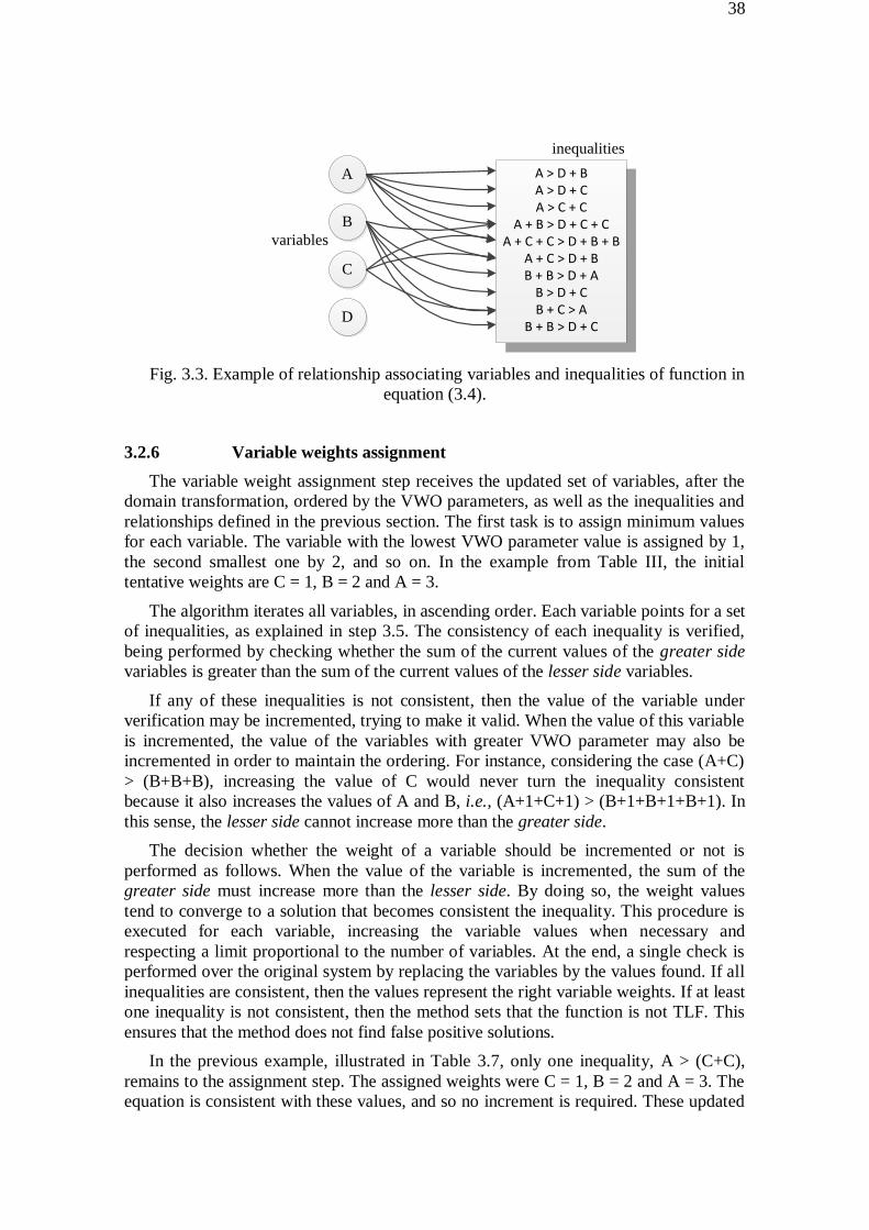
Figure 32 Inequalities simplification flow 42 Figure 33 Example of map associating variables and inequalities 45
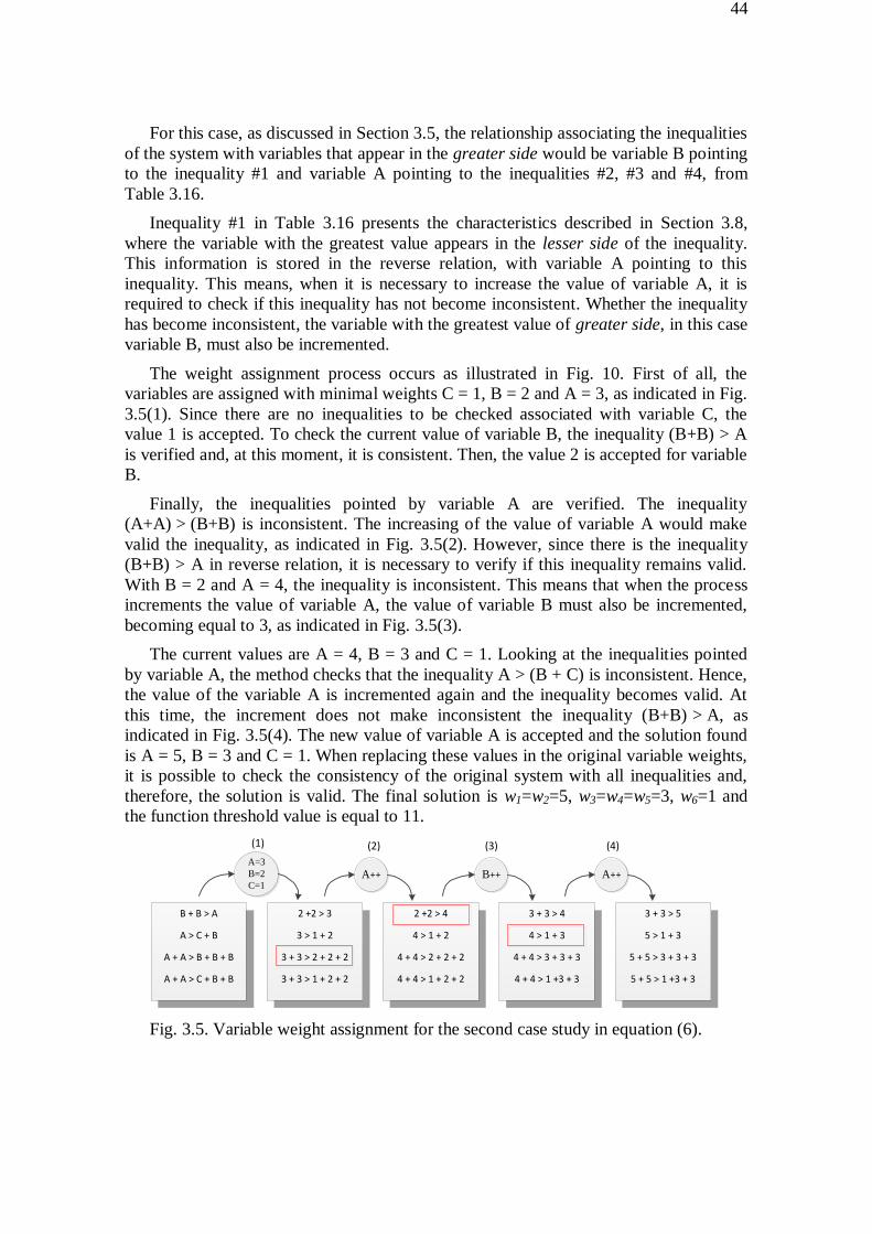
Figure 34 Variable weight assignment for the first example
ƒ=x1x2˅x1x3˅x1x4˅x2x3˅x2x4˅x1x5x6 46
Figure 35 Variables weights assignment for the second example 47 Figure 36 Average execution time per function for each number of variables using the 44-
6genlib set of functions 47
Figure 41 Example of initial bonded-pairs 49 Figure 42 Example of initial bonded-pairs 49 Figure 43 Bonded-pair association example 50 Figure 44 Combining the elements of a bucket new element are generated and stored in a new bucket 51 Figure 45 Some elements of Fig 44 can be removed to reduce the number of elements in a
bucket improving memory use and execution time 51 Figure 46 General flow of functional composition method 52 Figure 47 Bonded-pair representation for threshold networks 52 Figure 48 A naiumlve approach for associate TLGs 53 Figure 49 An improved way approach for associating TLG 53
7
Figure 410 Proposed way for associating TLGs 54 Figure 411 TLGs representing the functions f1 and f2 54 Figure 412 The naiumlve way for associating the functions f1 and f2 55 Figure 413 The proposed method for associating the functions f1 and f2 55 Figure 414 Algorithm flow of the proposed method 56 Figure 415 Synthesis flow of threshold logic circuits 57 Figure 416 Threshold logic circuit synthesis flow 60 Figure 417 Profile of MCNC Boolean network nodes 60 Figure 418 Profile of MCNC Boolean network nodes 61
8
LISTA OF TABLES
Table 11 Different functions implemented by adjusting the threshold value of the gate in Fig
11 13 Table 12 Main works addressing threshold logic circuit synthesis 18 Table 31 Relationship between the input weights and the function threshold value 41
Table 32 Greater side and lesser side sets 41
Table 33 Generated inequalities system 42 Table 34 Fake variables based in the variable Chowrsquos parameter 43
Table 35 Inequalities system with the fake variables 43
Table 36 Inequalities simplification for the given example 43 Table 37 Resultant set of inequalities 43
Table 38 Original inequalities system with the computed input weights 46
Table 39 Chowrsquos parameter values for the first example ƒ=x1x2˅x1x3˅x1x4˅x2x3˅x2x4˅x1x5x6 47
Table 310 Inequalities generation for the first example 48
Table 311 Original inequalities system for the first example 48
Table 312 Updated variable created for each Chowrsquos parameter value 48 Table 313 Simplified inequalities system 48
Table 314 Selected inequalities for the variable weight assignment step 49
Table 315 Updated variable crated for each Chowrsquos parameter value 50 Table 316 Simplified inequalities for the variable weight assignment step 50
Table 317 Number of TLFs identified by each method 52
Table 318 Number of TLFs classes identified for each method 52
Table 319 Average time per function for each number of variables 52 Table 320 Average time per function for each number of variables 53
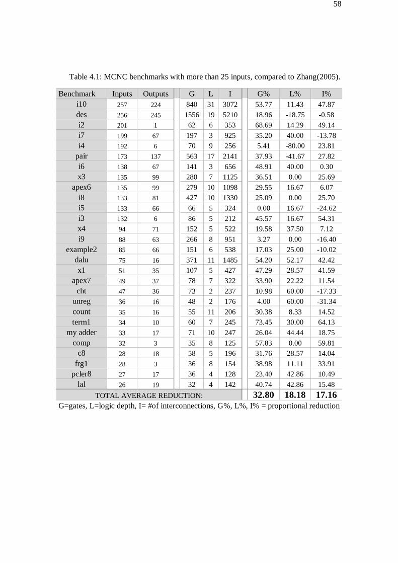
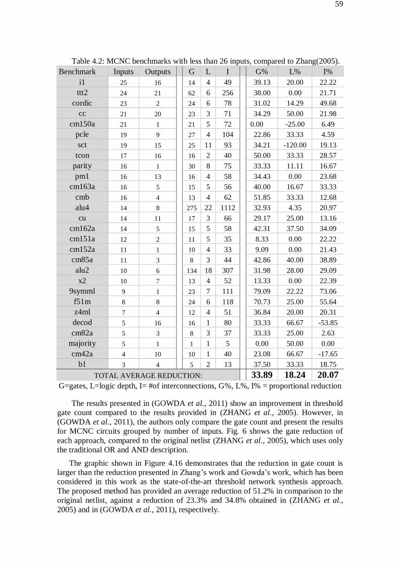
Table 41 MCNC benchmarks with more than 25 inputs compared to Zhang(2005) 58 Table 42 MCNC benchmarks with less than 26 inputs compared to Zhang(2005) 59 Table 43 MCNC circuit decompositions SIS and ABC tools 62
9
LIST OF ABBREVIATIONS AND ACRONYMS
AIG And Inverter Graph
ASIC Application Specific Integrated Circuit
BDD Binary Decision Diagram
CAD Computer Aided Design
CMOS Complementary Metal-Oxide-Semiconductor
CTL Capacitive Threshold Logic
EDA Electronic Design Automation
FC Functional Composition
FPGA Field programmable gate arrays
HDL Hardware Description Language
ILP Integer Linear Programming
ISOP Irredundant Sum-of-products
MAJ Majority gate
MOBILE Monostable-Bistable Logic Element
NCL Null Convention Logic
QCA Quantum Cellular Automata
ROBDD Reduced Ordered Binary Decision Diagram
RTD Resonant Tunneling Diode
RTL Register Transfer Level
SET Single Electron Transistor
SOP Sum-of-products
TLG Threshold Logic Gate
TLF Threshold Logic Function
VLSI Very Large Scale Integration
10
CONTENTS
ABSTRACT 4
RESUMO 5
LIST OF FIGURES 6
LISTA OF TABLES 8
1 INTRODUCTION 12
11 Motivation 13
12 Standard cell IC design flow 14 121 Logic synthesis in the standard cell flow 14
1211 Decomposition 15 1212 Pattern Matching 15 1213 Covering 16
13 Threshold logic design flow 16
14 Objectives 18
15 Thesis Organization 18
2 PRELIMINARES 19
21 Basic concepts 19 211 Boolean cofactors 19 212 Unateness 19 213 Irredundant sum-of-products 20 214 Threshold Logic Function 20 215 Threshold Logic Gate 20 216 Threshold Logic Functions Properties 21 217 Classes of Boolean function 21 218 Chowrsquos Parameters 22
22 TLG Physical Implementations 22 221 CMOS Threshold logic Latch 23 222 Spintronics 24 223 Memristors 24 224 Single Electron Tunneling (SET) 25 225 Quantum Cellular Automata (QCA) 26
11
226 NCL Threshold Logic for asynchronous circuits 27 2261 Transistor-Level Implementation 27
227 Resonant Tunneling Devices (RTD) 28
23 Final Considerations 29
3 THRESHOLD LOGIC IDENTIFICATION 30
31 Related Work 30
32 Proposed Method 31 321 Variable weight order 31 322 Generation of inequalities 32 323 Creation of inequalities system 34 324 Simplification of inequalities 35 325 Association of inequalities to variables 37 326 Variable weights assignment 38 327 Function threshold value calculation 39 328 Variable weights adjustment 39
33 Case studies 40 331 First case 40 332 Second case 43
34 Experimental Results 45 341 Identification effectiveness 45
35 Runtime efficiency 46 351 Opencore circuits 47
4 THRESHOLD LOGIC BASED CIRCUIT SYNTHESIS 48
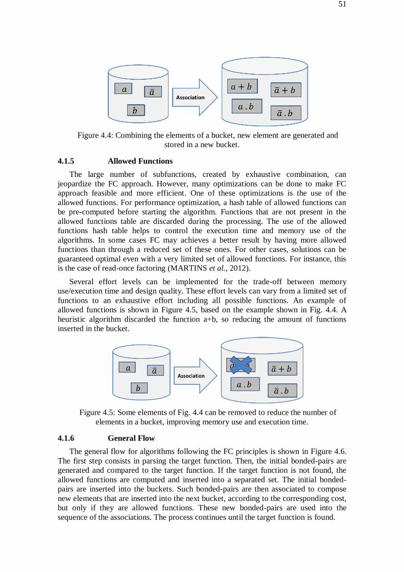
41 Functional Composition Method 48 411 Bonded-Pair Representation 49 412 Initial Functions 49 413 Bonded-Pair Association 50 414 Partial Order and Dynamic Programming 50 415 Allowed Functions 51 416 General Flow 51
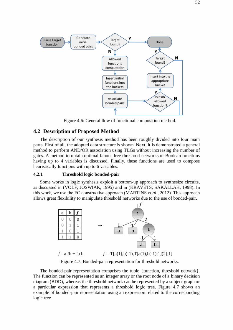
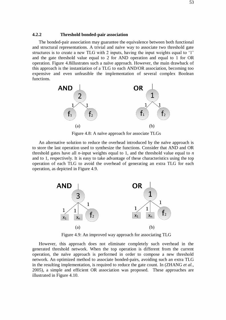
42 Description of Proposed Method 52 421 Threshold logic bonded-pair 52 422 Threshold bonded-pair association 53
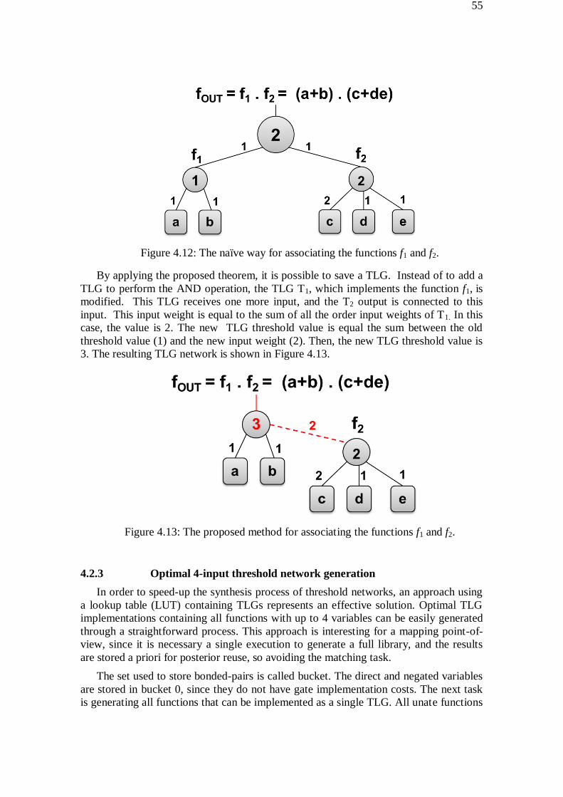
4221 Example of proposed threshold bonded-pair association 54 423 Optimal 4-input threshold network generation 55 424 Threshold network synthesis with up to 6 inputs 56
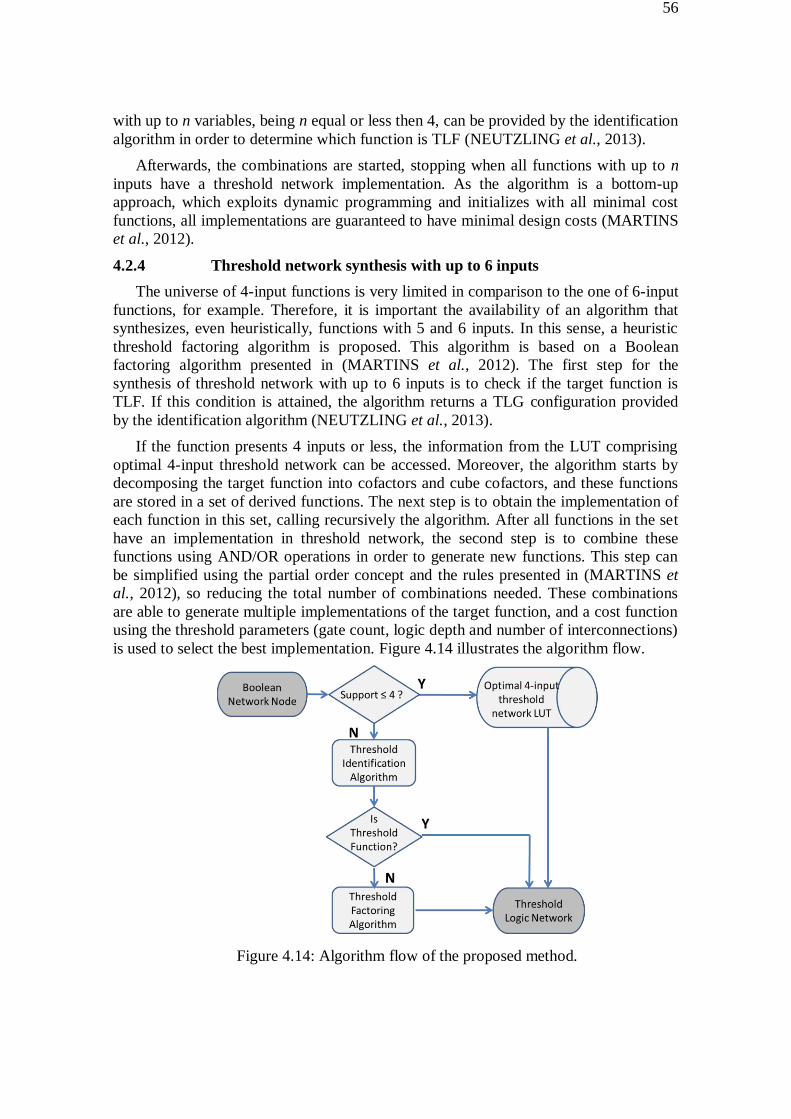
43 Experimental results 57
44 Future work 60
5 CONCLUSIONS 63
6 REFERENCES 64
12
1 INTRODUCTION
In the past five decades the transistor scaling has resulted in an exponential increase
of circuit integration (MOORE 1965) Development of integrated circuits (ICs) with
larger amount of transistors is the key for modern electronic products evolution
However according to the international technology roadmap for semiconductors
(ITRS) transistor scaling is becoming increasingly more difficult Nanoscale metal-
oxide semiconductor (MOS) devices start to be influenced by quantum physic effects
These challenges motivate the investigation of new alternatives to VLSI circuit design
(ITRS 2011)
Several technologies are emerging as alternatives to silicon complementary metal-
oxide-semiconductor (CMOS) transistor targeting greater level of miniaturization
reduced fabrication costs higher integration density and better performance These
nanotechnologies are based on different physical electrical magnetic and mechanical
phenomena They present distinct characteristics compared to CMOS technology
The most basic logic gates possible to implement in CMOS are NAND NOR and
INVERTER Some of future nanotechnologies use different logic styles For instance
the basic element of quantum cellular automata (QCA) technology is the majority logic
gate (ZHANG et al 2005) These differences represent a hard challenge for future IC
design that if well explored can lead to advantages over CMOS
Threshold logic functions (TLFs) are a subset of Boolean functions composed of
functions obeying the following principles First each input has a specific weight and
the gate has a threshold value Second the function output is defined by the ratio
between the sum of the weights of ON inputs and the threshold value of the gate if this
ratio is equal or greater than one than the output of the gate is one A Threshold logic
gate (TLG) implements a TLF Many complex Boolean functions can be implemented
in a single TLG and any Boolean function can be implemented using a TLG network
(MUROGA 1971)
In order to exploit the advantages of threshold logic in new technologies computer
aided design (CAD) tools that automate the design of integrated circuits directly on this
logical style are required The development of CAD tools for CMOS was essential to
the evolution of this technology There is an extra interest in the study of threshold
circuits because networks constructed with threshold gates are almost equivalent to
standard feed forward neural networks models using sigmoidal activation functions
and thus most of the properties and characteristics of the circuits can be extended and
applied to neural networks (BEIU et al 1996 SUBIRATS JEREZ FRANCO 2008)
The objective of this work is to develop methods for an integrated circuit design
flow based on threshold logic These methods should synthesize a TLG based circuit
13
implementation from a given Boolean network that composes a circuit The synthesis
should optimize given cost functions such as number of TLGs input weights and
number of interconnections in order to optimize the final circuit area and performance
11 Motivation
Static CMOS and pass transistor logic (PTL) are logic styles used in current digital
IC design based in MOS transistor From a functional point of view such logic styles
are able to implement any Boolean function in a single gate through series and parallel
associations (ignoring the inversions) Obviously electric characteristics like the
number of transistors in series limit the functions which are efficiently implemented
(WESTE HARRIS 2009)
Some logic styles suffer limitations on the set of functions that can be implemented
in a single gate For instance null convention logic (NCL) is able to implement only
threshold logic functions (TLF) In the other hand such logic style has potential benefits
in asynchronous IC design Logic styles proposed for emerging technologies like
memristors spintronics devices resonant tunneling devices (RTD) quantum cellular
automata (QCA) and single electron tunneling devices (SET) are also limited to
implement only TLFs
CAD tools currently used in digital IC design were developed to optimize CMOS
logic style based circuits Hence such tools do not explore specific TLF properties In
this sense TLG based circuits can be optimized when synthesized through CAD tools
focused in threshold logic (ZHANG et al 2005 GOWDA et al 2011)
An important property in TLGs is the possibility to implement different Boolean
functions only changing the weight inputs and the threshold value For instance Figure
11 presents a TLG implemented using RTDs where each RTD area corresponds to one
input weight or to the threshold value Suppose all the input weights be equal to 1 and
the threshold value equal to 5 It corresponds to the Boolean function f=abcde the five
input AND (AVEDILLO JM 2004) Decreasing the threshold value to 4 the gate
implements the function f=abcd+abce+abde+acde+bcde Table 11 shows different
functions can be implemented by keeping all input weights equal to 1 and just
decreasing the threshold value
Figure 11 TLG implemented using RTDs
Table 11 Different functions implemented by adjusting the threshold value of the
gate in Fig 11
threshold = 5 f=abcde
threshold = 4 f=abcd+abce+abde+acde+bcde
threshold = 3 f=abc+abd+abe+acd+ace+ade+bcd+bce+bde+cde
threshold = 2 f=ab+ac+ad+ae+bc+bd+be+cd+ce+de
14
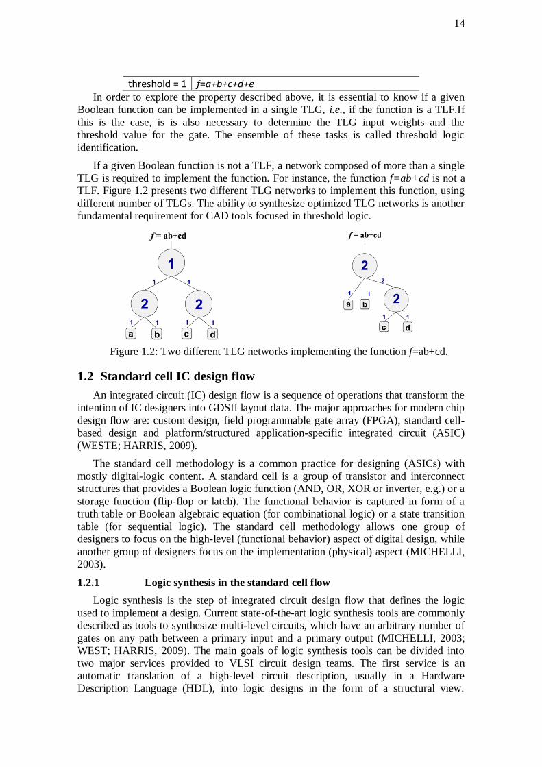
threshold = 1 f=a+b+c+d+e In order to explore the property described above it is essential to know if a given
Boolean function can be implemented in a single TLG ie if the function is a TLFIf
this is the case is is also necessary to determine the TLG input weights and the
threshold value for the gate The ensemble of these tasks is called threshold logic
identification
If a given Boolean function is not a TLF a network composed of more than a single
TLG is required to implement the function For instance the function f=ab+cd is not a
TLF Figure 12 presents two different TLG networks to implement this function using
different number of TLGs The ability to synthesize optimized TLG networks is another
fundamental requirement for CAD tools focused in threshold logic
Figure 12 Two different TLG networks implementing the function f=ab+cd
12 Standard cell IC design flow
An integrated circuit (IC) design flow is a sequence of operations that transform the
intention of IC designers into GDSII layout data The major approaches for modern chip
design flow are custom design field programmable gate array (FPGA) standard cell-
based design and platformstructured application-specific integrated circuit (ASIC)
(WESTE HARRIS 2009)
The standard cell methodology is a common practice for designing (ASICs) with
mostly digital-logic content A standard cell is a group of transistor and interconnect
structures that provides a Boolean logic function (AND OR XOR or inverter eg) or a
storage function (flip-flop or latch) The functional behavior is captured in form of a
truth table or Boolean algebraic equation (for combinational logic) or a state transition
table (for sequential logic) The standard cell methodology allows one group of
designers to focus on the high-level (functional behavior) aspect of digital design while
another group of designers focus on the implementation (physical) aspect (MICHELLI
2003)
121 Logic synthesis in the standard cell flow
Logic synthesis is the step of integrated circuit design flow that defines the logic
used to implement a design Current state-of-the-art logic synthesis tools are commonly
described as tools to synthesize multi-level circuits which have an arbitrary number of
gates on any path between a primary input and a primary output (MICHELLI 2003
WEST HARRIS 2009) The main goals of logic synthesis tools can be divided into
two major services provided to VLSI circuit design teams The first service is an
automatic translation of a high-level circuit description usually in a Hardware
Description Language (HDL) into logic designs in the form of a structural view
15
Additionally as a second service logic synthesis tools also try to optimize the resulting
circuit in terms of cost functions while satisfying design constraints required by the
designers Typical cost functions include chip area power consumption critical path
delay and the degree of testability of the final circuit Design constraints imposed by
users can include different timing requirements on different inputoutput paths required
frequency output loads etc (MICHELLI 2003 WEST HARRIS 2009 SASAO
1997 GEREZ 1999)
The logic synthesis step is commonly divided into two major tasks the technology
independent optimizations and the technology-dependent optimizations Figure 22
depicts the logic synthesis flow for cell-based VLSI circuit designs The main tasks
performed in the technology-independent stage are Boolean minimizations circuit
restructuring and local optimizations In the second stage the technology-dependent
one the generic circuit resulting from stage one is mapped to the standard cell library in
the technology mapping and trade-off optimizations are performed using all the
information from the characterized cells such as gate sizing delay optimizations on
critical paths buffer insertion and fanout limiting (SASAO 1997)
Technology mapping also known technology binding is an important phase in the
technology-dependent optimizations The technology mapping is the process by which
the technology-independent logic circuit is implemented in terms of the logic elements
available in a particular technology library of standard cells (MICHELLI 2003 WEST
HARRIS 2009 MARQUES et al 2009) Each logic element is associated with
information about delay area as well as internal and external capacitances The
optimization problem is to find an implementation meeting some user defined
constraints (as a target delay) while minimize other cost functions such as area and
power consumption This process is frequently described as being divided into three
main phases decomposition matching and covering (MICHELLI 2003 WEST
HARRIS 2009 MARQUES et al 2009)
1211Decomposition
In this phase the data structure for the technology mapping called subject graph is
created The specification of this new representation relies strongly on the mapping
strategy adopted Some approaches break the graph into trees Others focus on applying
structural transformations such that the subject graph has similar structural
representations as the cells from the library (MICHELLI 2003 WEST HARRIS 2009
MARQUES et al 2009) Another objective of this phase is to ensure each node of the
subject graph does have at least one match against the cells of the library Thus the
method assures that there exists a way to associate all portions of the subject to at least
one cell from the library thus guaranteeing a feasible solution
1212Pattern Matching
In the pattern matching phase the algorithms try to find a set of matches between
each node of the subject graph and the cells in the technology library Two main
approaches are commonly used described as follows (MICHELLI 2003 WEST
HARRIS 2009 MARQUES et al 2009)
Structural matching identifies common structural patterns between portions of the
subject graph and cells of the library Most approaches reduce the structural matching
problem to a graph isomorphism problem Due to the reduced size of cell graphs which
limit the portion of the subject graph to be inspected for graph isomorphism the
16
computational time to determining the isomorphism (commonly intractable) can be
neglected Boolean matching performs the matching considering Boolean functions of
the same equivalence class It usually performs the matching using binary decision
diagrams (BDD) by trying different variable orderings until a matching is found
Boolean matching is computationally more expensive than structural matching but can
lead to better results
1213Covering
Once the whole subject graph has been matched the final phase of technology
mapping needs to cover the entire logic network choosing among all the matches a
subset that minimizes the objective cost function and produce a valid implementation of
the circuit The cost function is often the total area the largest delay the total power
consumption or a composition of these (MICHELLI 2003 WEST HARRIS 2009
MARQUES et al 2009)
Technology mapping transforms the technology-independent circuit into a network
of gates from the given technology (library) The simple cost estimation performed in
previous steps is replaced by a more concrete implementation-driven estimation during
technology mapping These costs can be further reduced afterwards through technology
dependent optimizations Technology mapping is constrained by several factors such as
the availability of gates (logic functions) in the technology library the drivability of
each gate in its logic family and the delay power and area of each gate (MICHELLI
2003 MARQUES et al 2009)
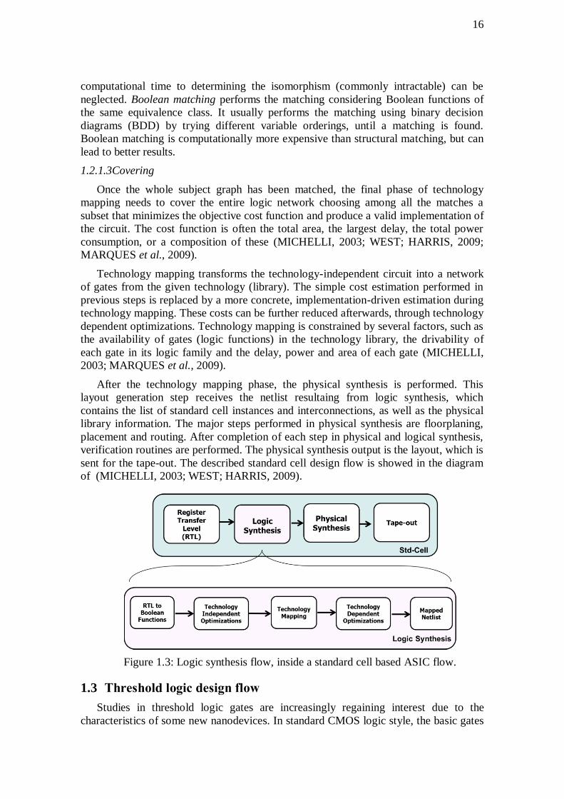
After the technology mapping phase the physical synthesis is performed This
layout generation step receives the netlist resultaing from logic synthesis which
contains the list of standard cell instances and interconnections as well as the physical
library information The major steps performed in physical synthesis are floorplaning
placement and routing After completion of each step in physical and logical synthesis
verification routines are performed The physical synthesis output is the layout which is
sent for the tape-out The described standard cell design flow is showed in the diagram
of (MICHELLI 2003 WEST HARRIS 2009)
Figure 13 Logic synthesis flow inside a standard cell based ASIC flow
13 Threshold logic design flow
Studies in threshold logic gates are increasingly regaining interest due to the
characteristics of some new nanodevices In standard CMOS logic style the basic gates
17
are INVERTER NAND and NOR However in some emerging technologies the most
basic logic gates which can be implemented are intrinsically threshold logic gates This
means that more complex Boolean functions can be implemented with the same cost of
implementing a NAND or NOR gate
However the current EDA tools are developed for standard CMOS circuits and are
not prepared to explore the benefits of the threshold logic Therefore it is necessary to
establish an alternative design flow that performs a threshold logic synthesis ie to find
an optimized circuit implementation composed of threshold logic gates
presents a proposal for threshold logic synthesis flow The RTL description is not
changed as well as the Boolean network elaboration Technology independent
optimizations are also performed by traditional academic tools such ABC
(BERKELEY 2013) and SIS (SENTOVICH et al 1992) The methods focused on
threshold logic synthesis start from the optimized Boolean network
The goal is to generate a TLGs netlist which implements the given Boolean
networks (which compose the complete circuit) The technology mapping does not use a
specific pre-characterized cell library An approach known as library-free mapping is
used where a set of allowed functions that can be used as cell is defined (REIS 1999
MARQUES et al 2007) The set of allowed functions in this case is defined by the
functions that are threshold logic ie functions that can be implemented by a single
TLG called threshold logic functions (TLF)
In order to perform such library-free technology mapping two methods are required
The first one must be able to determine if a given Boolean function is a TLF as well as
to compute the input weights and the threshold value This task is called threshold logic
identification The second method should be responsible for the technology mapping
seeking an implementation for the circuit that minimizes the cost functions such as the
number of TLGs and logic depth This task is called TLG network synthesis and the
result is a TLG netlist
The proposed logic synthesis methods do not restrict the physical implementation of
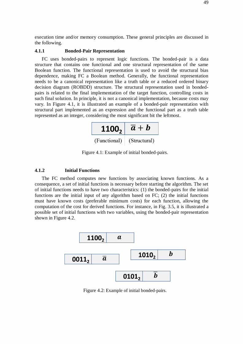
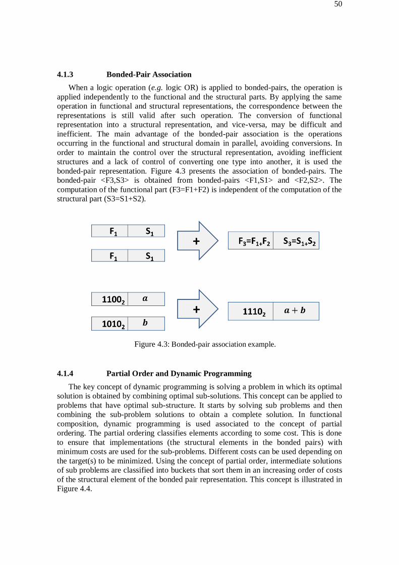
threshold logic gates to some specific technology It is possible to determine which cells
should be built to be used in the circuit Thereafter the physical synthesis can be
performed using either traditional place and routing methods or methods focused in
threshold logic or in the chosen nanotechnology
18
Figure 14 Threshold logic synthesis flow
14 Objectives
The major objective of this work is to propose methods to allow design flows that
explore benefits of TLFs Two methods are proposed and detailed in Chapters 3 and 4
The first contribution is a heuristic method to perform identification and synthesis of
TLFs The objective is to identify if a given Boolean function is TLF Such input
weights and threshold value must be calculated by the proposed method This task is
called TLF identification and determines if the given Boolean function can be
implemented as a single TLG
When there is no solution for the identification problem ie if the identification
method determines that the given Boolean function is not a TLF another method able
to synthesize TLG networks is required This is the second contribution of this work
The method is responsible to synthesize a group of interconnected TLGs which
implement the target Boolean function The synthesis should minimize the cost
functions like number of TLGs logic depth and number of interconnections The
proposed method is based on a principle called functional composition (FC) The
algorithm associates simpler sub-solutions with known costs in order to produce a
solution with minimum cost An optimized ANDOR association between threshold
networks is proposed and it allows the functional composition to reduce the cost
functions
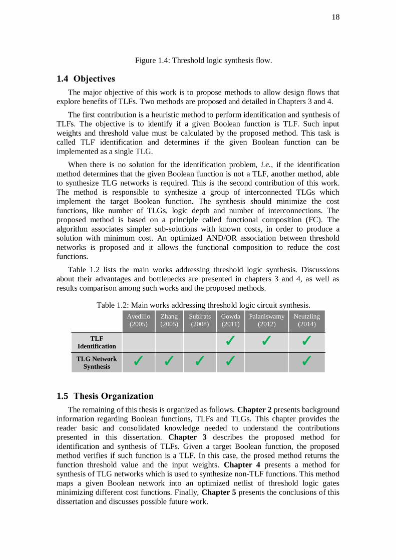
Table 12 lists the main works addressing threshold logic synthesis Discussions
about their advantages and bottlenecks are presented in chapters 3 and 4 as well as
results comparison among such works and the proposed methods
Table 12 Main works addressing threshold logic circuit synthesis Avedillo
(2005)
Zhang
(2005)
Subirats
(2008)
Gowda
(2011)
Palaniswamy
(2012)
Neutzling
(2014)
TLF
Identification
TLG Network
Synthesis
15 Thesis Organization
The remaining of this thesis is organized as follows Chapter 2 presents background
information regarding Boolean functions TLFs and TLGs This chapter provides the
reader basic and consolidated knowledge needed to understand the contributions
presented in this dissertation Chapter 3 describes the proposed method for
identification and synthesis of TLFs Given a target Boolean function the proposed
method verifies if such function is a TLF In this case the prosed method returns the
function threshold value and the input weights Chapter 4 presents a method for
synthesis of TLG networks which is used to synthesize non-TLF functions This method
maps a given Boolean network into an optimized netlist of threshold logic gates
minimizing different cost functions Finally Chapter 5 presents the conclusions of this
dissertation and discusses possible future work
19
2 PRELIMINARES
This chapter is organized into three main sections The first one presents some basic
concepts on threshold logic and logic synthesis These fundamentals are useful to
facilitate the understanding of this work The second part consists in a review of
threshold logic gates implementations that have been proposed in the literature based
on MOS transistors and nanodevices Finally two widespread application of threshold
logic gates are presented one using resonant tunneling diodes and another using null
convention logic style which serves as the basis for a kind of asynchronous circuits
21 Basic concepts
211 Boolean cofactors
Cofactor operation is a very basic and significant operation over Boolean functions
Let us define cofactor as the following
Let f Bn rarr B be a Boolean function and x = x0hellipxn the variables in support of f
The cofactor of f with respect to xi is denoted as f(x1hellipxi=chellipxn) where c isin 0 1
(BOOLE 1854) It is also possible to define as positive cofactor the operation where a
variable receive the Boolean constant 1 The opposite is defined as negative cofactor
and is when a variable receives the Boolean constant 0 For presentation sake let
f(x1hellipxi=chellipxn) equiv f(xi=c)
It is not an easy task to enumerate all methods that take advantage of the cofactor
operation One of the most important examples is the Shannon expansion where a
function can be represented as a sum of two sub-functions of the original (SHANNON
1948)
f (x1hellipxn) = xi middot f(xi=0) + xi middot f(xi=1) (22)
212 Unateness
The unateness behavior is an intrinsic characteristic of Boolean functions It enables
us to know the behavior of each variable as well the behavior of the entire function Let
f be a Boolean function The unateness behavior of a variable xi in f can be obtained
according to the following relations
α = f (xi=1) (23)
20
β = f (xi=0) (24)
γ = α + β (25)
dont care α equiv β (26) positive unate α equiv γ (27) negative unate β equiv γ (28) binate α ne β ne γ (29)
We say that a Boolean function is unate if all its variables are either positive or
negative unate In the case when at least one variable were binate the Boolean function
is considered binate Unate Boolean functions are of special interest for this work
Unateness is an important characteristic in the threshold logic identification All TLF
are unate functions Therefore if a function has binate variables the function cannot be
TLF The TLF identification method first of all verify the function unateness If a given
function is binate this function is not a TLF
213 Irredundant sum-of-products
An expression is called sum-of-products (SOP) when such expression corresponds to
product terms joined by a sum (OR) operation An irredundant sum-of-products (ISOP)
is a SOP where no product term can be deleted or simplified without changing the logic
behavior of the function Unate functions have unique ISOPs (BRAYTON et al 1984)
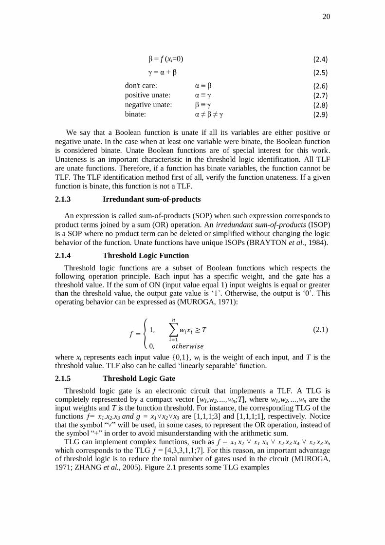
214 Threshold Logic Function
Threshold logic functions are a subset of Boolean functions which respects the following operation principle Each input has a specific weight and the gate has a threshold value If the sum of ON (input value equal 1) input weights is equal or greater than the threshold value the output gate value is lsquo1rsquo Otherwise the output is lsquo0rsquo This operating behavior can be expressed as (MUROGA 1971)
119891 = 1 sum119908119894119909119894
119899
119894=1
ge 119879
0 119900119905ℎ119890119903119908119894119904119890
(21)
where xi represents each input value 01 wi is the weight of each input and T is the threshold value TLF also can be called lsquolinearly separablersquo function
215 Threshold Logic Gate
Threshold logic gate is an electronic circuit that implements a TLF A TLG is completely represented by a compact vector [w1w2hellipwnT] where w1w2hellipwn are the input weights and T is the function threshold For instance the corresponding TLG of the functions ƒ= x1x2x3 and g = x1˅x2˅x3 are [1113] and [1111] respectively Notice that the symbol ldquo˅rdquo will be used in some cases to represent the OR operation instead of the symbol ldquo+rdquo in order to avoid misunderstanding with the arithmetic sum
TLG can implement complex functions such as ƒ = x1 x2 ˅ x1 x3 ˅ x2 x3 x4 ˅ x2 x3 x5 which corresponds to the TLG ƒ = [433117] For this reason an important advantage of threshold logic is to reduce the total number of gates used in the circuit (MUROGA 1971 ZHANG et al 2005) Figure 21 presents some TLG examples
21
Figure 21 Some examples of TLGs
216 Threshold Logic Functions Properties
All TLF are unate functions Therefore if a function has binate variables the function cannot be TLF However not all unate functions are TLF (MUROGA 1971) The function ƒ = (x1x2)˅(x3x4) is a simple example of unate function that is not TLF
If the given logic function contains negative variables these variables can be manipulated in the same way as functions having only positive variables in order to identify if it is a TLF or not If ƒ(x1x2hellipxn) is TLF defined by [w1w2hellipwnT] then its
complement 119891(x1x2hellipxn) is also TLF defined by [-w1-w2hellip-wn1-T] This process is illustrated in Figure 22
If a function is TLF and NOT gate (inverter) is available then it is possible to obtain a realization by using TLG with only positive weights by selectively negating the inputs (MUROGA 1971)
Figure 22 Threshold logic properties (MUROGA 1971)
217 Classes of Boolean function
Boolean functions can be grouped into classes of functions Given a set of all
functions with up to n variables they can be grouped in classes of functions As
illustrated in Figure 23 Boolean functions can be grouped considering the
complementation (negation) of its inputs (x) permutation of its inputs (y) andor
inversion (negation) of its output (z) The NP class represents the set of equivalent
functions obtained by negating and permuting the inputs (HINSBERGER KOLLA
1998)
Figure 23 Types of Boolean equivalence used to group functions in classes
(HINSBERGER KOLLA 1998)
22
218 Chowrsquos Parameters
Chowrsquos parameters are a particular set of parameters used to define the relationship
among the weights of TLF Given a function ƒ(x1x2hellipxn) we call mi the number of
entries for which ƒ(xi) = 1 and xi = 1 and ni the number of entries for which ƒ(xi) = 1
and xi = 0 The Chowrsquos parameter pi of a variable xi explained in (AVEDILLO JM
RUEDA 1999 MUROGA 1971) is given by
119901119894 = 2119898119894 minus 2119899119894 (210)
Figure 24 shows the Chowrsquos parameter computation using the function
f=x1x2˅x1x3x4 as example The correlation among pi and pj values of two the input
variables induces the correlation among the weights wi and wj of the input variables xi
and xj respectively If pi gt pj then wi gt wj (MUROGA 1971)
x1 x2 x3 x4 ƒ
0 0 0 0 0
0 0 0 1 0 m1 = 5 and n1 = 0
0 0 1 0 0 p1 = 10
0 0 1 1 0
0 1 0 0 0 m2= 4 and n2 = 1
0 1 0 1 0 p2 = 6
0 1 1 0 0
0 1 1 1 0 m3 = 3 and n3 = 2
1 0 0 0 0 p3 = 2
1 0 0 1 0
1 0 1 0 0 m4 = 3 and n4 = 2
1 0 1 1 1 p4 = 2
1 1 0 0 1
1 1 0 1 1
1 1 1 0 1
1 1 1 1 1
Figure 24 Calculating Chowrsquos parameters value for function f=x1x2˅ x1x3x4
22 TLG Physical Implementations
Researches on neural networks (NNs) go back sixty years ago The key year for the
development of the ldquoscience of mindrdquo was 1943 when the first mathematical model of a
neuron operating fashion the threshold logic gate was invented (MCCULLOCJ PITTS
1943) In the last decades the tremendous impetus of VLSI technology has made
neurocomputer design a really lively research topic Researches on hardware
implementations of NNs and on threshold logic in particular have been very active In
this section we will focus only on different approaches that have been tried for
implementing TLG in silicon Effectiveness of TLG as an alternative technology to
modern VLSI design is determined by the availability cost and capabilities of the basic
building blocks In this sense many interesting circuit concepts for developing CMOS
compatible TLGs have been explored As the number of different proposed solutions
reported in the literature is on the order of hundreds we cannot mention all of them
here Instead we shall try to cover important types of architectures and present several
representative examples (BEIU 2003)
23
Recently many other approaches have been used for implementing TLG charge-
coupled devices optical and even molecular (BEIU QUINTANA AVEDILLO 2003)
The main emerging future devices used to implement TLGs are the spintronics
memristors single electron tunneling (SET) resonant tunneling devices (RTDs)
quantum cellular automata (QCA) (ZHANG et al 2005) (GAO ALIBART
STRUKOV 2013)
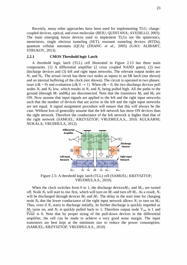
221 CMOS Threshold logic Latch
A threshold logic latch (TLL) cell illustrated in Figure 213 has three main
components (1) A differential amplifier (2 cross coupled NAND gates) (2) two
discharge devices and (3) left and right input networks The relevant output nodes are
N1 and N2 The actual circuit has these two nodes as inputs to an SR latch (not shown)
and an internal buffering of the clock (not shown) The circuit is operated in two phases
reset (clk = 0) and evaluation (clk 0 rarr 1) When clk = 0 the two discharge devices pull
nodes N5 and N6 low which results in N1 and N2 being pulled high All the paths to the
ground (through M7 andM8) are disconnected Note that the transistors M5 and M6 are
ON Now assume that input signals are applied to the left and the right input networks
such that the number of devices that are active in the left and the right input networks
are not equal A signal assignment procedure will ensure that this will always be the
case Without loss of generality assume that the left network has more ON devices than
the right network Therefore the conductance of the left network is higher than that of
the right network (SAMUEL KRZYSZTOF VRUDHULAS 2010 KULKARNI
NUKALA VRUDHULA 2012)
Figure 25 A threshold logic latch (TLL) cell (SAMUEL KRZYSZTOF
VRUDHULAS 2010)
When the clock switches from 0 to 1 the discharge devicesM11 and M12 are turned
off Node N5 will start to rise first which will turn on M7 and turn off M1 As a result N1
will be discharged through devices M5 and M7 The delay in the start time for charging
node N6 due the lower conductance of the right input network allows N1 to turn on M3
Thus even if N2 starts to discharge initially its further discharge is quickly impeded as
M3 turns on and N2 is quickly pulled back to 1 Therefore output node Vout is 1 and
119881119900119906119905 is 0 Note that by proper sizing of the pull-down devices in the differential
amplifier the cell can be made to achieve a very good noise margin The input
transistors are best kept at the minimum size to reduce the power consumption
(SAMUEL KRZYSZTOF VRUDHULAS 2010)
24
222 Spintronics
An architecture for threshold gate is based on the integration of conventional
MOSFETs and a Spintronic device known in the literature as Spin Transfer Torque -
Magnetic Tunneling Junction (STTMTJ) device (NUKALA KULKARNI
VRUDHULA 2012) The novel feature of this architecture is that the STT-MTJ device
is intrinsically a primitive threshold device ie it changes its state when the magnitude
of the current through the device exceeds some threshold value This simple property
when exploited leads to an extraordinary simple realization of a complex threshold
gate referred here as an STL cell
Recent works discuss the usage of STT-MTJ in logic computation such as (ZHAO
BELHAIRE CHAPPERT 2007) (GANG et al 2011) (PATIL et al 2010) All
previous works on STT-MTJ for logic use it for storage (logic 0 or 1) or as resistive
networks to perform single logic gates In contrast the method described in (NUKALA
KULKARNI VRUDHULA 2012) employs a single STT-MTJ device in conjunction
with MOSFETs to build complex threshold function and is illustrated in Figure 214
Figure 26 Spintronic Threshold Logic (STL) cell (NUKALA KULKARNI
VRUDHULA 2012)
The cell operates in the following manner The signals WR RD_i and PR are
pairwise complementary ie no two of them are in a high level at the same time
Initially PR is asserted and the current flows into the NMOS transistor (NM1) through
the STT-MTJ device from B to A The flow of current brings the STT-MTJ in the anti-
parallel or high resistance state When the WR is asserted certain amount of current (I)
flows through the STT-MTJ device depending on the number of ON PMOS transistors
(P1 to PN shown in Figure 214) If the current I is larger than a switching current Ic
then the STT-MTJ device switches to the low resistance state Otherwise it remains in
high resistance state This is the write phase of the cell When the WR pulse goes low
no current flows through the STT-MTJ device and since the device is non-volatile the
state is maintained
Reading the state of STT-MTJ is done by asserting the RD_i pulse When RD_i goes
high transistor NM3 whose source is connected to the STT-MTJ device and transistor
NM2 connected to the STT-Ref are enabled The drains nodes of these two transistors
N5 and N6 are the two outputs of the STL cell and they are connected to the sense
amplifier to evaluate the state of the STT-MTJ device
223 Memristors
Leon Chua (1971) proposed a fourth fundamental device the memristor which
relates charge q and flux φ in the following way
25
119872(119902) =119889(120593(119902))
119889119902 (211)
The parameter M(q) denotes the memristance of a charge controlled memristor
measured in ohms It has been observed that the memristance at any particular instance
depends on the integral of current or voltage through the device from negative infinity
to that instance Thus the memristor behaves like an ordinary resistor at any given
instance where its resistance depends on the complete history of the device (CHUA
1971 STRUKOV et al 2008 WILLIAMS 2008)
The key idea is to use memristors as weights of the inputs to a threshold gate For a
threshold gate using memristors as weights if Vi and Memi are the voltage and
memristance at the input i then the output Y is
119884 =
1 119894119891 sum119881119894
119872119890119898119894ge 119868119903119890119891
0 119894119891 sum119881119894
119872119890119898119894lt 119868119903119890119891
(212)
The voltages applied at the inputs of a TLG are converted into current values which
are then summed up by connecting all the wires together This sum of all weighted
currents is then compared with a threshold or reference current Iref The memristance
value can be selected by applying an appropriate voltage over a period of time A TLG
using memristors as weight is shown in Figure 215 (RAJENDRAN et al 2010)
Figure 27 MTL gate which uses the memristors as weights and Iref as the threshold
(RAJENDRAN et al 2010)
224 Single Electron Tunneling (SET)
SET has been receiving increased attention because it combines large integration
and ultra-low power dissipation (GHOSH JAIN SARKAR 2013) The use of SET
technology for TLGs has been advocated and several implementations have been
presented A basic minority SET gate is shown in Figure 216 It consists of a double-
junction box (CL and two Cj junctions) three input capacitors and an output capacitor
Vd is the bias voltage Three input voltages V1 V2 and V3 are applied to Node 1
through the input capacitors These capacitors form a voltage summing network and
produce the mean of their inputs at Node 1 The double-junction box produces the
minority-logic output on Node 1 by the following rule If the voltage at Node 1 exceeds
a threshold an electron will tunnel from the ground to Node 1 via Node 2 and make the
voltage at Node 1 negative Otherwise the voltage at Node 1 will remain positive
Logic 1 and 0 are represented by a positive and negative voltage of equal magnitude
An SET minority gate can also implement a two input NOR or a two-input NAND gate
26
by setting one of its inputs to an appropriate logic value (OYA et al 2002 ZHANG et
al 2005 SULIEMAN BEIU 2004)
Figure 28 Single Electron Tunneling (SET) minority gate
225 Quantum Cellular Automata (QCA)
The quantum cellular automata (QCA) have been one of the promising
nanotechnologies in the future The analysis and simulation of QCA circuits has many
challenges It involves larger computational complexity Quantum dots are
nanostructures created from standard semi conductive materials These structures are
modeled as quantum wells They exhibit energy effects even at distances several
hundred times larger than the material system lattice constant A dot can be visualized
as well Once electrons are trapped inside the dot it requires higher energy for electron
to escape Quantum dot cellular automata is a novel technology that attempts to create
general computational functionality at the nanoscale by controlling the position of
single electrons (WALUS BUDIMAN JULLIEN 2004 ZHANG et al 2004) The
fundamental unit of QCA is the cell created with four quantum dots positioned at the
vertices of a square (WALUS et al 2004) The electrons are quantum mechanical
particles They are able to tunnel between the dots in a cell The electrons in the cell that
are placed adjacent to each other will interact As a result the polarization of one cell
will be directly affected by the polarization of its neighbors
Figure 217 shows quantum cells with electrons occupying opposite vertices These
interaction forces between the neighboring cells are able to synchronize their
polarization Therefore an array of QCA cells acts as wire and it is able to transmit
information from one end to another Thus the information is coded in terms of
polarization of cell Polarization of each cell depends on polarization of its neighboring
cells To perform logic computing we require universally a complete logic set We need
a set of Boolean logic gates that can perform AND OR NOT and FANIN and FAN
OUT operations The combination of these is considered as universal because any
general Boolean function can be implemented with the combination of these logic
primitives The fundamental method for computing is building a majority gate
(WALUS et al 2004 ZHANG et al 2004 ZHANG et al 2005)
Figure 29 Quantum Cellular Automata majority gate (ZHANG et al 2005)
The majority gate produces an output that reflects the majority of the inputs The
majority function is a part of a larger group of functions called threshold functions
27
Threshold functions work according to inputs that reaches certain threshold value before
output is asserted The majority function is most fundamental logic gate in QCA
circuits In order to create an AND gate we simply fix one of the majority gate input to
0 (P = -1) To create OR gate we fix one of inputs to 1 P = +1 The inverter or NOT gate
is also simple to implement using QCA (WALUS BUDIMAN JULLIEN 2004)
226 NCL Threshold Logic for asynchronous circuits
NULL Convention Logic (NCL) is a clock-free delay-insensitive logic design
methodology for digital systems (FANT 2005 MOREIRA et al 2014) Unlike
previous asynchronous design approaches NCL circuits are very easy to design and
analyze In NCL a circuit consists of an interconnection of primitive modules known as
M-of-N threshold gates with hysteresis All functional blocks including both
combinational logic and storage elements are constructed out of these same primitives
The designer simply specifies an interconnection of library modules in order to obtain a
desired computational functionality The circuit operates at the maximum speed of the
underlying semiconductor device technology (SMITH DI 2009)
The primitive element that we consider is an M-of-N threshold gate with hysteresis
which we refer to as simply an M-of-N gate The abstract symbol for an M-of-N gate is
shown in Figure 218 The cases of interest are those where M le N An M-of-N gate is a
generalization of both Muller C-element and Boolean OR gate Specifically for N gt 1
an N-of-N gate corresponds to an N-input Muller C-element On the other hand a 1-of-
N gate corresponds to an N-input Boolean OR gate The cases where both M gt 1 and M
lt N are novel and have no counterparts in the literature (FANT 2005 MALLEPALLI
et al 2007)
Figure 210 General structure of a M-of-N NCL gate (MALLEPALLI et al 2007)
The M-of-N gates operate on signals that can have two possible abstract values
which we refer to as DATA and NULL In the normal mapping arrangement DATA
corresponds to a logic-1 voltage level while NULL corresponds to a logic-0 voltage
level The reverse mapping is also possible as are mappings into units of current
There are two important aspects of the M-of-N gate namely threshold behavior and
hysteresis behavior The threshold behavior means that the output becomes DATA if at
least M of the N inputs have become DATA The hysteresis behavior means that the
output only changes after a sufficiently complete set of input values have been
established In the case of a transition to DATA the output remains at NULL until at
least M of the N inputs become DATA In the case of a transition to NULL the output
remains at DATA until all N of the inputs become NULL (SMITH DI 2009)
2261Transistor-Level Implementation
NCL threshold gates are designed with hysteresis state-holding capability such that
after the output is asserted all inputs must be ldquodeassertedrdquo before the output will be
ldquodeassertedrdquo Therefore NCL gates have both set and hold equations where the set
equation determines when the gate will become asserted and the hold equation
28
determines when the gate will remain asserted once it has been asserted The set
equation determines the gate functionality as one of the 27 NCL gates (subset of
threshold functions)[f] whereas the hold equation is the same for all NCL gates and is
simply all inputs ORed together The general equation for an NCL gate with output f is
f=set+ 119891 bull hold) where 119891 is the previous output value and f is the new value Take the
TH23 gate for example The set equation is AB + AC + BC and the correspondent hold
equation is A + B + C therefore the gate is asserted when at least 2 inputs are asserted
and it then remains asserted until all inputs are deasserted (MALLEPALLI et al 2007)
NCL gates can also be implemented in a semi-static fashion where a weak feedback
inverter is used to achieve hysteresis behavior which only requires the set and reset
equations to be implemented in the NMOS and PMOS logic respectively The semi-
static TH23 gate is shown in Figure 220 In general the semi-static implementation
requires fewer transistors but it is slightly slower because of the weak inverter Note
that TH1n gates are simply OR gates and do not require any feedback such that their
static and semi-static implementations are exactly the same
Transistor-level libraries have been created for both the static and semi-static
versions of all the NCL gates used in the design For the static version minimum widths
were used for all transistors to maximize gate speed However for the semistatic
version larger transistors were required to overcome the weak feedback inverter to
obtain proper gate functionality and reduce the propagation delay (MALLEPALLI et
al 2007)
Figure 211 Semi-static CMOS implementation of a TH23 gate f = AB+AC+BC
(MALLEPALLI et al 2007)
227 Resonant Tunneling Devices (RTD)
RTDs can be considered the most mature type of quantum devices which are used
in high-speed and low-power circuits (CHOI et al 2009 PETTENGHI AVEDILLO
QUINTANA 2008) They operate at room temperature and have an IIIndashV large scale
integration process (SUDIRGO et al 2004 LITVINOV 2010) The incorporation of
RTDs into transistor technologies offers the opportunity to improve the speed and
compactness of large scale integration RTDs exhibit a negative differential resistance
(NDR) region in their currentndashvoltage characteristics which can be exploited to
increase the functionality implemented by a single gate significantly It reduces the
circuit complexity in comparison to conventional MOS technologies (AVEDILLO
QUINTANAROLDAN 2006)
29
RTD-based circuits rely on utilizing a threshold logic gate called monostablendash
bistable logic element (MOBILE) which combines a pair of series connected RTDs with
hetero junction field-effect transistors (HFETs) to achieve inputndashoutput isolation and
functionality (MAEZAWA MIZUTANI 1993) A series connection of three or more
RTDs which is a multi-threshold-threshold gate (MTTG) has been employed to
implement more complex functions than TLG Compared to the Boolean logic TLG
and MTTG can increase circuit functionality and reduce circuit levels and gate numbers
[8] To support the design of RTD gates various RTD models have been proposed in
The MOBILE shown in Figure 221(a) is a rising edge triggered current controlled
gate which consists of two RTDs connected in series and it is driven by a switching
bias voltage Vclk When Vclk is low both RTDs are in the on-state S0 and the circuit is
mono-stable as shown in Fig 222(b) When Vclk increases to an appropriate value it
ensures that the RTD with smaller peak current switches first from the ON-state to the
OFF-state The MOBILE can reach two possible states S1 and S2 which is referred to
bistable as shown in Fig 222(c) (WEI SHEN 2011) Output becomes stable at S1 and
generates a low value if the load RTD has a smaller peak current Otherwise the output
switches to S2 with a high value Logic functionality can be achieved by embedding an
input stage which modifies the peak current of one of the RTDs (BHATTACHARYA
MAZUMDER 2001)
(a) (b) (c)
Figure 212 MOBILE (a) basic circuit (b) monostable state and (c) bistable state
(WEI SHEN 2011)
23 Final Considerations
This chapter presented several proposals to implement TLGs using different devices
and structures In order to explore the features of threshold logic an IC design flow with
algorithms focused in this logic style is necessary Chapters 3 and 4 present methods to
address two crucial steps of a TLG based design flow
30
3 THRESHOLD LOGIC IDENTIFICATION
An essential task to establish a design flow based on threshold logic gates (TLG) is
to determine whether a Boolean function is a threshold logic function (TLF) ie if the
function can be implemented using a single TLG Furthermore threshold logic
identification aims to find the correct TLG which implements the Boolean function by
calculating the corresponding input weight and the threshold value of the gate
In this chapter a new method for threshold logic identification is proposed Section
31 reviews the related methods and presents a brief discussion about each strategy
Section 32 explains in detail each step of the proposed method and Section 33
demonstrates two practical examples to demonstrate it Finally Section 34 presents
experimental results comparing to the results from the state-of-the-art approaches in
this field The efficiency in the number of identified TLF and runtime of each method is
verified
31 Related Work
Most of methods proposed for threshold logic identification aims to solve a system
of inequalities generated from the truth table using integer linear programming ILP
(AVEDILLO JM 2004 ZHANG et al 2005 SUBIRATS JEREZ FRANCO 2008)
ILP provides optimal results However such a strategy becomes unfeasible when the
number of variables increases because the number of inequalities to be solved increases
exponentially with the number of input variables Heuristic methods on the other hand
are not optimal but present a significant improvement in execution time
The first heuristic (non-ILP) method known to identify threshold logic functions was
proposed by Gowda et al in (GOWDA VRUDHULA KONJEVOD 2007) and
improved afterwards in (GOWDA VRUDHULA 2008) and (GOWDA et al 2011)
This method is based on functional decomposition and a min-max factorization tree
The target function is decomposed into simpler subfunctions until they can be directly
characterized (AND OR 0 1) These subfunctions are merged by respecting some TLF
properties The main limitation of this method is the reduced number of TLF identified
Moreover it represents a very time consuming process and presents a strong
dependence to the initial expression structure including the ordering of the initial tree
In (PALANISWAMY GOPARAJU TRAHOUDAS 2010) it is presented a
method based on the modified Chowrsquos parameters The basic idea is assign to each
input a weight value that is proportional to the Chowrsquos parameter This method has been
later improved in (PALANISWAMY GOPARAJU TRAHOUDAS 2012) and can be
considered as the state-of-the-art work in TLF identification However the bottlenecks
of these approaches are also the number of identified functions and the fact that the
31
assigned input weights are not always the minimum possible values Those non-
minimal weights can impact the final circuit area (ZHANG et al 2005)
32 Proposed Method
In the proposed method a complete system of inequalities is also built using similar
strategy to ILP inequalities generation algorithms However unlike ILP-based
approaches the inequalities system is not actually solved Instead the algorithm selects
some of the inequalities as constraints to the associated variables to compute the
variable weights in a bottom-up way After this assignment the consistency of the
complete system is verified in order to check if the weights have been correctly
computed
As mentioned before if a function is not unate then it is not TLF Therefore the
algorithm first checks the unateness property of the function A negative variable can be
changed to a positive one if the weight signal is inverted and this amount is subtracted
from the threshold value Without loss of generality the proposed algorithm starts from
a positive unate function
For a better understanding the algorithm has been split into eight steps which are
illustrated in Fig 31 and summarized in the following in step (1) the ordering of the
variable weights is identified step (2) generates the inequalities step (3) creates the
system of inequalities in step (4) the simplification of the inequalities set is executed
in step (5) the association of each variable to some inequalities is performed step (6)
assigns the variable weights and the consistency of the solution found is verified if the
given Boolean function is confirmed as TLF then the threshold value is calculated in
step (7) in step (8) is performed an eventual adjusting of the variable weights when it is
necessary
Variable ordering
computation
Inequalities system
generation
Simplification of
inequalities
Weight assignment
and result
consistency check
Unate Boolean
function
Variable weight
adjustment
Association of
inequalities for
each variable
Threshold
Logic Function
parameters
Step (1) Step (2) Step (4)
Step (5)Step (6)Step (7)Step (8)
Creation of
inequalities
Step (3)
Function threshold
value computation
Fig 31 Flow chart of the proposed algorithm for TLF identification
321 Variable weight order
In the proposed method is essential to know the variable weight ordering since this
information is used in the inequalities simplification and weight assignment steps A
well-known manner to obtain such an ordering is through the Chowrsquos parameters
32
[Chow 1961 Muroga 1971] The correlation between the Chowrsquos parameters pi and pj
of two variables xi and xj induces the correlation between the respective weights wi and
wj ie if pi gt pj then wi gt wj [Muroga 1971]
A new algorithm to obtain a variable weight ordering (WVO) parameter is proposed
WVO parameters provide similar variable weight ordering of Chowrsquos parameter
although the absolute parameter values are possibly different The proposed WVO
parameters are calculated directly from the ISOP and being simpler and faster to
compute Such parameters are based on max literal computation proposed in [Gowda et
al 2011]
Given an ISOP representation of a function f the largest variable weight of the
target TLF is associated to the literal that occurs most frequently in the largest cubes of f
(ie the cubes with fewer literals) In the case of a tie it is decided by comparing
frequency of the literals in the next smaller size cubes
The proposed algorithm defines for each cube a kind of weight corresponding to the
cube size Such weight is added to the VWO parameter of the variables present in the
cube The variable weight ordering is associated to the ordering of these VWO
parameters computed for each variable The pseudo algorithm of this step is described
in Algorithm 1 The time complexity of Algorithm 1 is O(mn) being m the number of
cubes and n the number of variables
Algorithm 1 Compute the variable weight order
Input function f with n variables represented by an ISOP F with cube set C that contains m cubes Output list VWO parameters list_VWO in ascending order
1 initialize all values of list_VWO as zero
2 for each cube c isin C do 3 lit = |c|
4 for each xi isin c do
5 add mn-lit in list_ VWO[xi] 6 end for 7 end for 8 order(list_ VWO) 9 return list_ VWO
For instance for the given Boolean function defined by the following ISOP
ƒ = (x1x2)˅(x1x3x4) (31)
the calculated values of variables x1 x2 x3 and x4 are 6(22+2
1) 4(2
2) 1(2
1) and
1(21) respectively whereas the Chowrsquos parameters of this variables would be 10 6 2
and 2 respectively Notice that the same ordering is obtained in both calculations Thus
in this case the algorithm initially assigns the weight of the variables x3 and x4 then
afterwards the weight of the variable x2 is assigned being the weight of variable x1 the
last one to be defined
322 Generation of inequalities
Equation (1) defines the relationship between the variable weights and the threshold
value of a TLF If the function value is true (lsquo1rsquo) for certain assignment vector then the
sum of weights of this assignment is equal to or greater than the threshold value
Otherwise the function value is false (lsquo0rsquo) ie the sum of weights is less than the
threshold value From this relationship it is possible to generate the inequalities
associated For instance given the truth table of the function from equation (3) the
relationship between variable weights and the threshold value is shown in Table I
33
Table 31 Inequalities from truth table representing function defined by equation
(31)
x1 x2 x3 x4 ƒ Inequality
0 0 0 0 0 0 lt T 0 0 0 1 0 w4 lt T 0 0 1 0 0 w3 lt T
0 0 1 1 0 (w3 + w4) lt T 0 1 0 0 0 w2 lt T 0 1 0 1 0 (w2 + w4) lt T 0 1 1 0 0 (w2 + w3) lt T
0 1 1 1 0 (w2 + w3 + w4) lt T 1 0 0 0 0 w1 lt T 1 0 0 1 0 (w1 + w4) lt T
1 0 1 0 0 (w1 + w3) lt T 1 0 1 1 1 (w1 + w3 + w4) ge T 1 1 0 0 1 (w1+ w2) ge T
1 1 0 1 1 (w1+ w2 + w4) ge T 1 1 1 0 1 (w1 + w2 + w3) ge T 1 1 1 1 1 (w1 + w2 + w3 + w4) ge T
Some relationships in Table I are redundant due to the fact that some inequalities are
self-contained into another inequalities For instance since we havethe relation
(w1+w2) ge T and the variable weights are always positive so the relation
(w1+w2+w3) ge T is redundant The irredundant information is the lesser assignments
(ie the lesser weight sum) that make the function true (lsquo1rsquo) and the greater
assignments (ie the greater weight sum) that make it false (lsquo0rsquo) Notice that an
assignment vector A(a1a2a3an) is smaller than or equal to an assignment vector
B(b1b2b3hellipbn) denoted as A le B if and only if ai le bi for (i = 123hellipn) For example
the assignment vector (1001) is lesser than the assignment vector (1101) whereas
the assignment vectors (0101) and (1100) are not comparable
In our method these redundancies are avoided using two ISOP expressions one for
the direct function and another for the negated function In the example the least true
assignment vectors are (1100) and (1011) and the greatest false assignment vectors
are (1010) (1001) and (0111) Therefore the algorithm creates only (w1+w2) and
(w1+w3+w4) in the greater side and (w1+w3) (w1+w4) and (w2+w3+w4) in the lesser
side The ISOP from f and frsquo are considered as inputs of the method Each sum of
variable weights greater than the function threshold value is placed in the greater side
set whereas each sum of weights which is less than the threshold value belongs to the
lesser side set Table 32 shows these two sets for the illustrative example in equation
(31)
Table 32 Greater side and lesser side sets for function described in Table 31
greater side lesser side
(w1+w2) ge T gt (w1+w4)
(w1+w3+w4) ge T gt (w1+w3)
---
T gt (w2+w3+w4)
This procedure is described by the pseudo algorithm in Algorithm 2 The time
complexity of Algorithm 2 is O(m+mrsquo) where m is the number of cubes in the ISOP of
function f and mrsquo is the number of cubes in the ISOP of the negated function f rsquo
34
Algorithm 2 Generation of inequalities sides
Input ISOP form of function f and negated function f rsquo Output two sets of inequalities sides a set ineq_greater and a set ineq_lower
1 for each cube c isin C
2 create inequality_side S from c
add S in ineq_greater 3 end for 4 for each cube c isin C rsquo
5 create inequality_side S from c add S in ineq_lower 6 end for 7 return ltineq_greater ineq_lowergt
323 Creation of inequalities system
The pseudo algorithm that represents the creation of the system of inequalities is
presented in Algorithm 3 The instruction compose_inequality creates a new inequality
from the two inequality sides Each greater side element is greater than each lesser side
element because the greater side elements are greater than (or equal to) the threshold
value whereas the lesser side elements are smaller than that The inequalities system is
generated by performing a kind of Cartesian product of the greater side set and the
lesser side set
Table 33 shows the six inequalities generated for the Boolean function illustrated in
Table 31 Notice that if the procedure had taken into account all truth table
assignments 55 inequalities would be generated The time complexity of Algorithm 3 is
O(mmrsquo) where m is the number of cubes in the ISOP of function f and mrsquo is the
number of cubes in the ISOP of negated function f rsquo
Table 33 Inequalities system generated for function described in Table 32
Inequality
1 (w1+w2) gt (w1+w4)
2 (w1+w2) gt (w1+w3)
3 (w1+w2) gt (w2+w3+w4)
4 (w1+w3+w4) gt (w1+w4)
5 (w1+w3+w4) gt (w1+w3)
6 (w1+w3+w4) gt (w2+w3+w4)
Algorithm 3 Inequalities generation
Input two sets of inequalities a set ineq_greater and a set ineq_lower
Output set of inequalities ineq_set
1 set_ineq = empty
2 for each inequality_side g isin ineq_greater
3 for each inequality_side l isin ineq_lower
4 ineq = compose_inequality(gl) 5 add ineq in set_ineq
6 end for 7 end for 8 return ltset_ineqgt
35
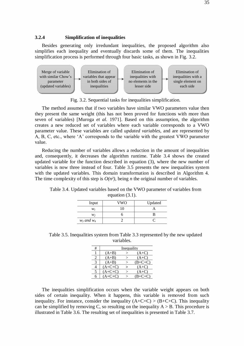
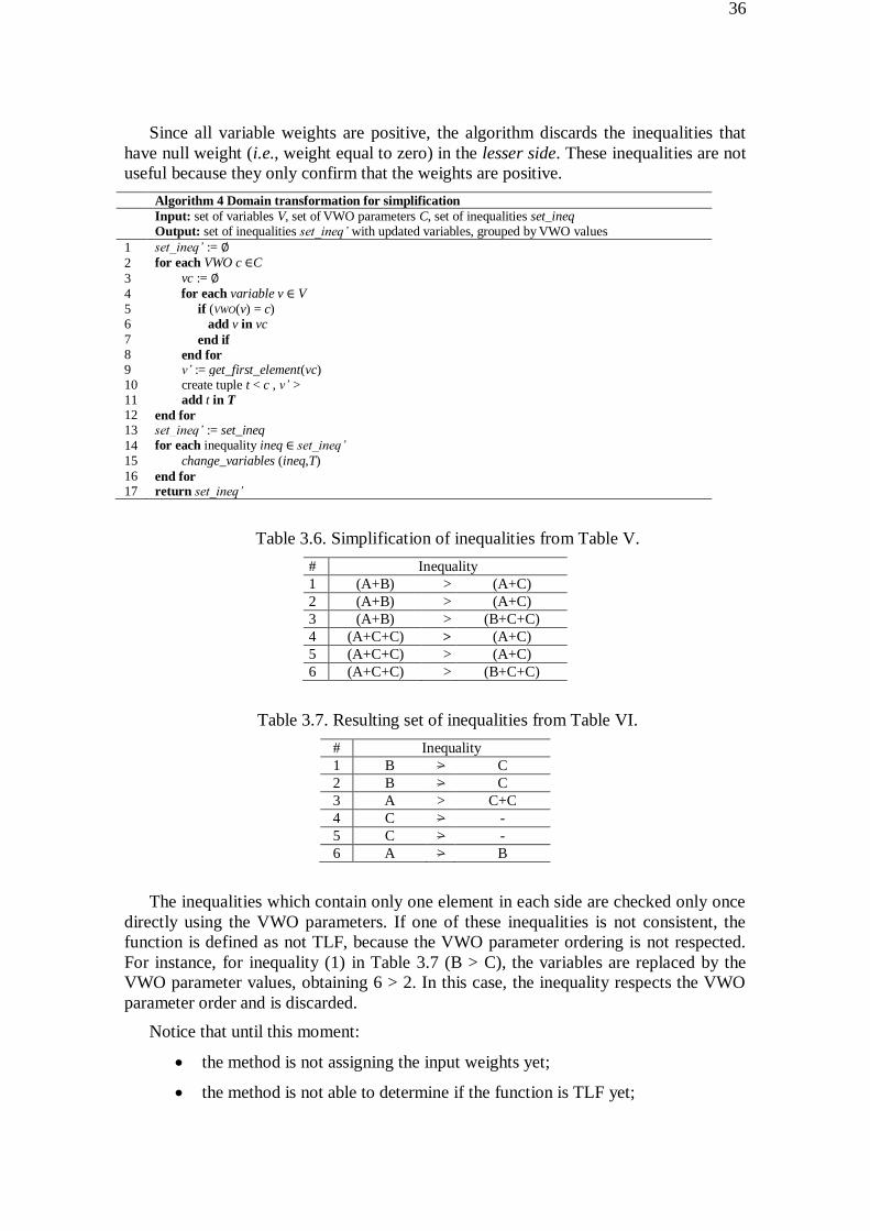
324 Simplification of inequalities
Besides generating only irredundant inequalities the proposed algorithm also
simplifies each inequality and eventually discards some of them The inequalities
simplification process is performed through four basic tasks as shown in Fig 32
Merge of variable
with similar Chowrsquos
parameter
(updated variables)
Elimination of
variables that appear
in both sides of
inequalities
Elimination of
inequalities with
no elements in the
lesser side
Elimination of
inequalities with a
single element on
each side
Fig 32 Sequential tasks for inequalities simplification
The method assumes that if two variables have similar VWO parameters value then
they present the same weight (this has not been proved for functions with more than
seven of variables) [Muroga et al 1971] Based on this assumption the algorithm
creates a new reduced set of variables where each variable corresponds to a VWO
parameter value These variables are called updated variables and are represented by
A B C etc where lsquoArsquo corresponds to the variable with the greatest VWO parameter
value
Reducing the number of variables allows a reduction in the amount of inequalities
and consequently it decreases the algorithm runtime Table 34 shows the created
updated variable for the function described in equation (3) where the new number of
variables is now three instead of four Table 35 presents the new inequalities system
with the updated variables This domain transformation is described in Algorithm 4
The time complexity of this step is O(nsup2) being n the original number of variables
Table 34 Updated variables based on the VWO parameter of variables from
equation (31)
Input
weight
VWO
parameter
Updated
variable w1 10 A
w2 6 B
w3 and w4 2 C
Table 35 Inequalities system from Table 33 represented by the new updated
variables
Inequality 1 (A+B) gt (A+C)
2 (A+B) gt (A+C) 3 (A+B) gt (B+C+C) 4 (A+C+C) gt (A+C)
5 (A+C+C) gt (A+C) 6 (A+C+C) gt (B+C+C)
The inequalities simplification occurs when the variable weight appears on both
sides of certain inequality When it happens this variable is removed from such
inequality For instance consider the inequality (A+C+C) gt (B+C+C) This inequality
can be simplified by removing C so resulting on the inequality A gt B This procedure is
illustrated in Table 36 The resulting set of inequalities is presented in Table 37
36
Since all variable weights are positive the algorithm discards the inequalities that
have null weight (ie weight equal to zero) in the lesser side These inequalities are not
useful because they only confirm that the weights are positive
Algorithm 4 Domain transformation for simplification
Input set of variables V set of VWO parameters C set of inequalities set_ineq
Output set of inequalities set_ineqrsquo with updated variables grouped by VWO values
1 set_ineqrsquo = empty
2 for each VWO c isinC
3 vc = empty
4 for each variable v isin V
5 if (VWO(v) = c) 6 add v in vc
7 end if 8 end for 9 vrsquo = get_first_element(vc) 10 create tuple t lt c vrsquo gt 11 add t in T
12 end for 13 set_ineqrsquo = set_ineq
14 for each inequality ineq isin set_ineqrsquo
15 change_variables (ineqT)
16 end for 17 return set_ineqrsquo
Table 36 Simplification of inequalities from Table V
Inequality
1 (A+B) gt (A+C)
2 (A+B) gt (A+C)
3 (A+B) gt (B+C+C)
4 (A+C+C) gt (A+C)
5 (A+C+C) gt (A+C)
6 (A+C+C) gt (B+C+C)
Table 37 Resulting set of inequalities from Table VI
Inequality
1 B gt C
2 B gt C
3 A gt C+C
4 C gt -
5 C gt -
6 A gt B
The inequalities which contain only one element in each side are checked only once
directly using the VWO parameters If one of these inequalities is not consistent the
function is defined as not TLF because the VWO parameter ordering is not respected
For instance for inequality (1) in Table 37 (B gt C) the variables are replaced by the
VWO parameter values obtaining 6 gt 2 In this case the inequality respects the VWO
parameter order and is discarded
Notice that until this moment
the method is not assigning the input weights yet
the method is not able to determine if the function is TLF yet
37
it is only possible to determine some functions that have been identified as
non TLF
After all these simplifications the set of useful inequalities can be significantly
reduced In the demonstration example described in Table 31 the only remaining
inequality is the number 3 in Table 37 A gt (C+C) which will be the only inequality to
be used in the assignment step The reduction in the number of inequalities is one of the
key points of the proposed method since the weight assignment is based on inequalities
manipulation However such a simplification becomes the method heuristic ie some
discarded inequality could be essential for the correct solution It generates false
negatives for functions with more than six variables The pseudo algorithm of the
complete inequalities simplification process is shown in Algorithm 5 The time
complexity of this step is O(nlog(n)mmrsquo) being n the number of variables m the
number of cubes in the ISOP of function f and mrsquo is the number of cubes in the ISOP of
the negated function f rsquo
Algorithm 5 Inequalities simplification
Input set of inequalities set_ineq
Output simplified set of inequalities set_ineq_simplified
1 set_ineq_simplified = empty
2 for each inequality ineq isin set_ineq
3 split ineq in greater and lesser side
4 for each variable v1 isin greater_side
5 for each variable v2 isin lesser_side 6 if (v1 = v2)
7 remove(v1 greater_side) 8 remove(v2 lesser_side) 9 end if 10 end for 11 end for 12 if lower_side is not empty
13 ineq = compose_inequality (greaterlesser) 14 add ineq in set_ineq_simplified
15 end if 16 end for 17 return set_ineq_simplified
325 Association of inequalities to variables
Before computing the variable weights the tuple ltvariablesinequalitiesgt
associating the variables with some of the inequalities is created By making so each
variable points to inequalities in which the variable is present on the greater side This
relationship is exploited in the weight assignment step discussed in the next section
However the function defined by equation (33) used as example in the description of
previous steps is not appropriate to illustrate how this procedure because the simplified
set has only one inequality For a better visualization of this step in Fig33 is shown an
example of one of this kind of relationship for the following function
ƒ =(x1x2x3)˅(x1x2x4)˅(x1x3x4)˅(x1x2x5)˅(x1x3x5)˅(x1x4x5)˅(x1x2x6)
˅(x1x3x6)˅( x2x3x4)˅(x2x3x5) (34)
38
A
B
C
A gt D + BA gt D + CA gt C + C
A + B gt D + C + CA + C + C gt D + B + B
A + C gt D + BB + B gt D + A
B gt D + CB + C gt A
B + B gt D + CD
variables
inequalities
Fig 33 Example of relationship associating variables and inequalities of function in
equation (34)
326 Variable weights assignment
The variable weight assignment step receives the updated set of variables after the
domain transformation ordered by the VWO parameters as well as the inequalities and
relationships defined in the previous section The first task is to assign minimum values
for each variable The variable with the lowest VWO parameter value is assigned by 1
the second smallest one by 2 and so on In the example from Table III the initial
tentative weights are C = 1 B = 2 and A = 3
The algorithm iterates all variables in ascending order Each variable points for a set
of inequalities as explained in step 35 The consistency of each inequality is verified
being performed by checking whether the sum of the current values of the greater side
variables is greater than the sum of the current values of the lesser side variables
If any of these inequalities is not consistent then the value of the variable under
verification may be incremented trying to make it valid When the value of this variable
is incremented the value of the variables with greater VWO parameter may also be
incremented in order to maintain the ordering For instance considering the case (A+C)
gt (B+B+B) increasing the value of C would never turn the inequality consistent
because it also increases the values of A and B ie (A+1+C+1) gt (B+1+B+1+B+1) In
this sense the lesser side cannot increase more than the greater side
The decision whether the weight of a variable should be incremented or not is
performed as follows When the value of the variable is incremented the sum of the
greater side must increase more than the lesser side By doing so the weight values
tend to converge to a solution that becomes consistent the inequality This procedure is
executed for each variable increasing the variable values when necessary and
respecting a limit proportional to the number of variables At the end a single check is
performed over the original system by replacing the variables by the values found If all
inequalities are consistent then the values represent the right variable weights If at least
one inequality is not consistent then the method sets that the function is not TLF This
ensures that the method does not find false positive solutions
In the previous example illustrated in Table 37 only one inequality A gt (C+C)
remains to the assignment step The assigned weights were C = 1 B = 2 and A = 3 The
equation is consistent with these values and so no increment is required These updated
39
variable values are assigned to the corresponding variable weights resulting in w1=3
w2=2 and w3=w4=1 Table 38 shows the original system with the assigned values
Table 38 Original system from Table 36 with the computed variable weights
Inequality
1 (3+2) gt (3+1)
2 (3+2) gt (3+1)
3 (3+2) gt (2+1+1)
4 (3+1+1) gt (3+1)
5 (3+1+1) gt (3+1)
6 (3+1+1) gt (2+1+1)
Since all inequalities are consistent the computed values are accepted as a valid
solution of the system Algorithm 6 shows the pseudo algorithm of the assignment step
The time complexity of this step is O(nmmrsquo) being n the number of variables m the
number of cubes in the ISOP of function f and mrsquo is the number of cubes in the ISOP of
the negated function f rsquo
Algorithm 6 Weights assignment
Input list of variables list_variables relationship of variables and associated inequalities set_ineq Output set of variables v with assigned values
1 n = 1 2 correct = false 3 for all variable v isin list_variables do
4 v = n 5 n= n++ 6 end for 7 for each variable v isin list_variables do
8 set_ineq = get_ineq_by_variable (v)
9 for each inequation ineq isin set_ineq
10 correct = verify_consistency(ineq) 11 while (correct = false OR v lt limit) 12 v = v++
13 increment_greater_variables(v list_variables)
14 correct = verify_consistency(ineq) 15 end while 16 end for 17 end for 18 return list_weight_VWO
327 Function threshold value calculation
After checking whether the weights have been assigned correctly the algorithm
calculates the function threshold value In a TLF represented through an ISOP form the
sum of weights of the variables contained in each product is equal to or greater than the
function threshold value Therefore the threshold value is equal to the least sum of
weights of the greater side set In the example defined by equation (3) and in Table I
the threshold value is 5 obtained from the greater side element of any inequality in
Table 38 (in this case all greater sides have equal sum) The final solution for such a
given Boolean function is [32115]
328 Variable weights adjustment
When a variable is incremented an already checked inequality can become
inconsistent One way to identify and prevent the occurrence of this problem is
explained in the following
40
For instance for a given function let us consider that the growing ordering of the
updated variable is D C B and A where A has the highest weight value and D has the
lowest weight value At a certain time the algorithm has checked the inequalities
associated to D C and B variables The inequalities associated with variable A are
checked and an inconsistency determines that the value of this variable needs to be
incremented However there is an inequality (B+C+D) gt A that has already been
checked By increasing the value of variable A the inequality that had been considered
consistent can become inconsistent
This kind of problem can occur when a variable in the lesser side of the inequality
has greater value than any variable value in the greater side In our investigation it was
observed that this occurs in less than 2 of the 6-input functions and never occurs in
functions with fewer variables As the consequence in these cases the minimum weight
values are not guaranteed
In order to solve this problem a relationship represented by the tuple
ltvariableinequalitiesgt where variables point to inequalities similarly as presented in
step (5) and is called reverse relation If a variable x is on the lesser side and its VWO
parameter value is greater than any VWO parameter of the greater side variables then
this information is recorded on the relationship tuple In the assignment step (6) when
the method specifies that a variable must be incremented this reverse relation may also
be consulted
At the moment of incrementing a variable the method
checks if there is an inequality associated to this variable in the reverse relation
checks if this inequality becomes inconsistent after the increment of variable x
(if so) increments the greatest value variable of the greater side and makes the
inequality consistent again This is done recursively for the variables with VWO
greater than the VWO of variable x
It is important to notice that whenever the value of some variable is incremented
the value of the higher variables must also be incremented ie the ordering must be
maintained A demonstration of this improvement is presented in Section 332
33 Case studies
In the previous section the method proposed for threshold logic function
identification was described The example from equation (12) used to demonstrate the
algorithms is quite simple having been adopted just to simplify the explanation and
facilitate the understanding of the procedure steps However the importance and impact
of each step can be subestimated with such a simple example In this section two more
complex functions are used as case studies to illustrate the main gains and benefits of
our approach
331 First case
Let us consider the following function
ƒ=(x1x2)˅(x1x3)˅(x1x4)˅(x2x3)˅(x2x4)˅(x1x5x6) (35)
The first step is to compute the VWO parameter for each variable and sort them as
shown in Table 39
41
Table 39 VWO parameter values for function of equation (5)
VWO parameter Variables 2 x5 x6
14 x4 x3 30 x2 34 x1
The given function described in equation (35) presents 64 possible assignment
vectors since it has six variables Among these assignments 23 are false and 41 are true
If all truth table assignments are taken into account then the system comprises 943
inequalities However as it was discussed before the method considers the ISOP
expression as input and generates only the greatest false assignments and the least true
assignments The greater side and lesser side sets for this case are presented in Table
310 Afterwards the Cartesian product between the greater side and the lesser side is
performed and 24 inequalities are obtained as showed in Table 311 In the next the
algorithm creates the updated variables based on repeated VWO parameters and
replaces the variable weights as shown in Table 312 The simplification is then
performed by removing variables that appear in both sides of the inequalities The
simplified set of inequalities is shown in Table 313
Table 310 Inequalities generation for the first case study in equation (5)
Greater side Lesser side
w1 + w2
gt T gt
w3 + w4 + w5 + w6
w1 + w3 w2 + w5 + w6
w1 + w4 w1 + w6
w2 + w3 w1 + w5
w2 + w4 ---
w1 + w5 + w6 ---
Table 311 Original inequalities system for the first case study in equation (5)
Inequality Inequality
1 w1+w2 gt w3+w4+w5+w6 13 w2+w3 gt w3+w4+w5+w6
2 w1+w2 gt w2+w5+w6 14 w2+w3 gt w2+w5+w6
3 w1+w2 gt w1+w6 15 w2+w3 gt w1+w6
4 w1+w2 gt w1+w5 16 w2+w3 gt w1+w5
5 w1+w3 gt w3+w4+w5+w6 17 w2+w4 gt w3+w4+w5+w6
6 w1+w3 gt w2+w5+w6 18 w2+w4 gt w2+w5+w6
7 w1+w3 gt w1+w6 19 w2+w4 gt w1+w6
8 w1+w3 gt w1+w5 20 w2+w4 gt w1+w5
9 w1+w4 gt w3+w4+w5+w6 21 w1+w5+w6 gt w3+w4+w5+w6
10 w1+w4 gt w2+w5+w6 22 w1+w5+w6 gt w2+w5+w6
11 w1+w4 gt w1+w6 23 w1+w5+w6 gt w1+w6
12 w1+w4 gt w1+w5 24 w1+w5+w6 gt w1+w5
Table 312 Updated variable created for each VWO parameter value for the first
case study in equation (5)
Variable
weights
VWO
parameter
Updated
variable w1 34 A w2 30 B
w3 and w4 14 C w5 and w6 2 D
42
For the variable weight assignment the method selects only inequalities that have
more than one weight in the lesser side and discards repeated inequalities Table XIV
presents the selected inequalities for the given example We have only 8 inequalities
against 943 inequalities whether a conventional method would be used and against 24
inequalities present in the original generated system
Table 313 Simplified inequalities system from Table XI using updated variables
from Table 312
1 A+B gt C+C+D+D 13 B gt C+D+D
2 A gt D+D 14 C gt D+D
3 B gt D 15 B+C gt A+D
4 B gt D 16 B+C gt A+D
5 A gt C+D+D 17 B gt C+D+D
6 A+C gt B+D+D 18 C gt D+D
7 C gt D 19 B+C gt A+D
8 C gt D 20 B+C gt A+D
9 A gt C+D+D 21 A gt C+C
10 A+C gt B+D+D 22 A gt B
11 C gt D 23 D gt
12 C gt D 24 D gt
Table 314 Selected inequalities from Table 313 for the variable weight
assignment step
1 A+B gt C+C+D+D 13 B gt C+D+D
2 A gt D+D 14 C gt D+D
5 A gt C+D+D 15 B+C gt A+D
6 A+C gt B+D+D 21 A gt C+C
Fig 9 illustrates the variable weight assignment At first the variables are assigned
with minimum values respecting the ordering defined by the respective VWO
parameters These values are A = 4 B = 3 C = 2 and D = 1 as indicated in Fig 34(1)
Since there are any inequality pointed by variable D the method accepts the value 1 for
such variable and starts to verify the inequalities pointed by C This way the inequality
13 from Table XIV turns to be not consistent and so increasing the variable value of C
this inequality becomes consistent as indicated in Fig 34(2) The updated value of
variable C is 3 and with this value all of the inequalities containing variable C are
consistent
C++
A+Bgt C+C+D+D
Agt D+D
Agt C+D+D
A+Cgt B+D+D
Bgt C+D+D
Cgt D+D
B+Cgt A+D
Agt C+C
B++ B++
A=4
B=3
C=2
D=1
(1)
(2) (3) (4)
4+3gt 2+2+1+1
4gt 1+1
4gt 2+1+1
4+2gt 3+1+1
3gt 2+1+1
2gt 1+1
3+2gt 4+1
4gt 2+2
5+4gt 3+3+1+1
5gt 1+1
5gt 3+1+1
5+3gt 4+1+1
4gt 3+1+1
3gt 1+1
4+3gt 5+1
5gt 3+3
6+5gt 3+3+1+1
6gt 1+1
6gt 3+1+1
6+3gt 5+1+1
5gt 3+1+1
3gt 1+1
5+3gt 6+1
6gt 3+3
7+6gt 3+3+1+1
7gt 1+1
7gt 3+1+1
7+3gt 6+1+1
6gt 3+1+1
3gt 1+1
6+3gt 7+1
7gt 3+3
Fig 34 Variable weight assignment for the first case study in equation (35)
43
Next the method checks the inequalities pointed by B The verification concludes
that the inequality 14 from Table XIV is inconsistent Incrementing once the value of
variable B does not become the inequality valid as indicated in Fig 34(3) but
decreases the difference between the sums of the two sides The increment is performed
again and the current values are B = 6 and A = 7 as indicated in Fig34 (4) making all
inequalities pointed by B becomes consistent Finally the method checks the
inequalities pointed by A and verifies that such inequalities are also valid with the
weights A = 7 B = 6 C = 3 and D = 1
After computing all variable weights the algorithm identify the function threshold
value The value is obtained from the least sum of weights value in the greater side set
In this case the threshold value is equal to 9 from any of the weight sums in Table 311
(w2 + w4) (w2 + w3) or (w1 + w5 + w6)
The final check is then performed over the original inequalities system presented in
Table 311 (ie before the simplification) with the assigned variable weights All
inequalities are verified consistent so the right solution found is w1 = 7 w2 = 6 w3 = 3
w4 = 3 w5 = 1 w6 = 1 and T = 9
Due to the bottom-up characteristic of our approach the variable weights and
function threshold value found are the minimum possible It is a quite relevant feature
since impacts directly on the area of corresponding TLG In the Palaniswamyrsquos method
[2012] for instance the solution found for the same TLF is [98441111]
332 Second case
A second case study is presented to demonstrate the eventual improvement
discussed in Section 38 exploiting the reverse relation concept Let us consider the
Boolean function represented by the following ISOP
f = (x1x2x3)˅(x1x2x4)˅(x1x3x4)˅(x1x2x5)˅(x1x3x5)˅(x1x4x5)˅(x1x2x6)
˅(x2x3x4)˅(x2x3x5)˅(x2x4x5) (36)
Table 315 shows the relationship between the variable weights the corresponding
VWO parameters and the created updated variables
Table 315 Updated variable created for each VWO parameter value of the second
case study in equation (6)
Variable
weights
VWO
parameter
Updated
variable w1 w2 34 A w3 w4 w5 30 B w6 14 C
To simplify such explanation the process of generation and simplification of
variables is not presented Table 316 shows the system using the updated variables
already simplified
Table 316 Simplified inequalities for the weight assignment step of the second case
study in equation (6)
1 B+B gt A
2 A gt C+B
3 A+A gt B+B+B
4 A+A gt C+B+B
44
For this case as discussed in Section 35 the relationship associating the inequalities
of the system with variables that appear in the greater side would be variable B pointing
to the inequality 1 and variable A pointing to the inequalities 2 3 and 4 from
Table 316
Inequality 1 in Table 316 presents the characteristics described in Section 38
where the variable with the greatest value appears in the lesser side of the inequality
This information is stored in the reverse relation with variable A pointing to this
inequality This means when it is necessary to increase the value of variable A it is
required to check if this inequality has not become inconsistent Whether the inequality
has become inconsistent the variable with the greatest value of greater side in this case
variable B must also be incremented
The weight assignment process occurs as illustrated in Fig 10 First of all the
variables are assigned with minimal weights C = 1 B = 2 and A = 3 as indicated in Fig
35(1) Since there are no inequalities to be checked associated with variable C the
value 1 is accepted To check the current value of variable B the inequality (B+B) gt A
is verified and at this moment it is consistent Then the value 2 is accepted for variable
B
Finally the inequalities pointed by variable A are verified The inequality
(A+A) gt (B+B) is inconsistent The increasing of the value of variable A would make
valid the inequality as indicated in Fig 35(2) However since there is the inequality
(B+B) gt A in reverse relation it is necessary to verify if this inequality remains valid
With B = 2 and A = 4 the inequality is inconsistent This means that when the process
increments the value of variable A the value of variable B must also be incremented
becoming equal to 3 as indicated in Fig 35(3)
The current values are A = 4 B = 3 and C = 1 Looking at the inequalities pointed
by variable A the method checks that the inequality A gt (B + C) is inconsistent Hence
the value of the variable A is incremented again and the inequality becomes valid At
this time the increment does not make inconsistent the inequality (B+B) gt A as
indicated in Fig 35(4) The new value of variable A is accepted and the solution found
is A = 5 B = 3 and C = 1 When replacing these values in the original variable weights
it is possible to check the consistency of the original system with all inequalities and
therefore the solution is valid The final solution is w1=w2=5 w3=w4=w5=3 w6=1 and
the function threshold value is equal to 11
A++
B + B gt A
A gt C + B
A + A gt B + B + B
A + A gt C + B + B
2 +2 gt 3
3 gt 1 + 2
3 + 3 gt 2 + 2 + 2
3 + 3 gt 1 + 2 + 2
2 +2 gt 4
4 gt 1 + 2
4 + 4 gt 2 + 2 + 2
4 + 4 gt 1 + 2 + 2
3 + 3 gt 4
4 gt 1 + 3
4 + 4 gt 3 + 3 + 3
4 + 4 gt 1 +3 + 3
3 + 3 gt 5
5 gt 1 + 3
5 + 5 gt 3 + 3 + 3
5 + 5 gt 1 +3 + 3
B++ A++
A=3
B=2
C=1
(1) (2) (3) (4)
Fig 35 Variable weight assignment for the second case study in equation (6)
45
34 Experimental Results
Three sets of experiments were carried out in order to validate and compare our
results to the ones from existing related algorithms available in the literature In the first
experiment the efficiency of the proposed method is evaluated in terms of the number
of TLF identified The execution time of the method is evaluated in the second
experiment calculating the average runtime per identified function In the third
experiment the functions (k-cuts) identified in the synthesis of opencores used as
benchmarking are analyzed for both the effectiveness and the runtime of TLF
identification The platform used was Intel Core i5 processor with 2GB main memory
341 Identification effectiveness
The main goal of threshold logic function identification methods is to maximize the
number of TLF identified representing their effectiveness The enumeration of all TLF
with up to eight variables has been already calculated by Muroga in [1970] being used
as reference in this work
In [2008] Gowda et al presented the first method to identify TLF without using
linear programming afterwards improving it in [2011] The approach presented by
Palaniswamy et al in [2012] provides better results Table 317 shows the
experimental results
Table 317 Number of TLF identified by each method
Number of
variables
Muroga
[1970]
Gowda
[2008]
Palaniswamy
[2012]
Proposed
method
TLF TLF TLF TLF
1 2 2 100 2 100 2 100 2 8 8 100 8 100 8 100 3 72 72 100 72 100 72 100 4 1536 1248 813 1536 100 1536 100 5 86080 36800 428 75200 874 86080 100 6 14487040 1447040 100 9424000 651 144870
40
100
For functions with up to three variables all mentioned methods identify 100 of
existing TLF Moreover Gowdarsquos method identifies 813 and 428 of four and five
variables respectively For functions with five and six variables Palaniswamyrsquos method
identified 874 and 651 of TLF respectively whereas our method identified
correctly all existing ones in both sets To the best of our knowledge that is the first
non-ILP method able to identify correctly all TLF with up to six inputs
As for more than six variables the set of functions becomes impractical to be
evaluated we used the NP representative class of functions The results are shown in
Table XVIII Notice that for all the universe of TLF with seven variables our approach
identifies almost 80 of them whereas the other methods identify less than 35
46
Table 318 Number of TLF identified for each method considering NP
representative class of functions
Number
of variables
Muroga
[1970]
Gowda
[2008]
Palaniswamy
[2012] Proposed method
TLF TLF TLF TLF
1 1 1 100 1 100 1 100 2 2 2 100 2 100 2 100 3 5 5 100 5 100 5 100 4 17 15 882 17 100 17 100 5 92 52 565 84 913 92 100 6 994 181 182 728 732 994 100 7 28262 573 20 9221 326 22477 795
35 Runtime efficiency
In the second experiment the execution time was evaluated by calculating the
average runtime spent to identify each TLF The results are shown in Table XIX These
values demonstrate that the proposed method is comparable to the Palaniswamyrsquos
method [2012] For all NP functions up to seven variables the average execution time
to identify each function was less than one millisecond
The time complexity of the method is dominated by the inequality simplification
performed in step 34 The time complexity of such a computation is O(nlog(n)mmrsquo)
being n the number of variables m the number of cubes in the ISOP of function f and
mrsquo is the number of cubes in the ISOP of the negated function f rsquo The scalability of our
method has been verified through a random set of five thousand threshold logic
functions from eight to eleven variables also shown in Table 319
Table 319 Average runtime per TLF identification for each number of variables
Number of variables 1 2 3 4 5 6 7 8 9 10 11
Runtime (milliseconds) 03 02 03 04 05 04 06 07 07 08 09
When the number of variables increases solving the inequalities system by linear
programming becomes quite expensive Fig 36 illustrates the scalability of our
heuristic method in comparison to the exponentially behavior of ILP approaches The
results were obtained taking into account the set of functions lsquo44-6genlibrsquo which
comprises 3503 unate functions with up to sixteen variables [Stentovich et al 1992]
Notice that the average runtime per function is presented for subsets of different number
of variables and in a logarithm scale in Fig 36
The ILP method execution time has a significant increase from eight variables and
reaches tens of seconds for sixteen variables On the other hand the proposed approach
spends only few milliseconds for this number of variables The difference is about four
orders of magnitude This benchmark is composed by functions which are the basis of
standard cells libraries and therefore are widely used by technology mapping engines
in the logic synthesis of digital integrated circuits Our method identifies correctly all
TLF in this set emphasizing again the algorithm effectiveness
47
Fig 36 Average runtime per function for number of variables considering the set
of unate Boolean functions lsquo44-6genlibrsquo [Stentovich et al 1992]
351 Opencore circuits
In the last experiment the cut enumeration was performed using the ABC tool
[Berkeley 2014] over six opencore circuits [Pistorius et al 2007] generating a set of
366 million of Boolean functions with up to 11 variables A profile summarizing the
number of TLF found by both the proposed method and ILP-based method is presented
in Table XX
Table 320 Analysis of k-cuts (n-variable functions) obtained from the synthesis of
opencores circuits
k Cuts Unate
(unatetotal)
TLF - ILP
(TLFunate)
TLF - proposed
(proposedILP)
Runtime (ms)
(ILP)
Runtime (ms)
(proposed)
2 90 72 (80) 72 (100) 7 (100) 046 008 (18) 3 1613 637 (39) 637 (100) 637 (100) 044 009 (21) 4 28169 9818 (35) 8227 (84) 8227 (100) 047 010 (20)
5 180166 82891 (46) 53216 (64) 53216 (100) 056 011 (19) 6 446580 208278 (47) 99976 (48) 99976 (100) 075 012 (16) 7 624192 252042 (40) 101039 (40) 101023 (99) 119 017 (14) 8 654727 233872 (36) 86708 (37) 86671 (99) 203 025 (12)
9 605959 190054 (31) 68872 (36) 68619 (99) 418 048 (12) 10 568520 158133 (28) 57176 (36) 56852 (99) 976 160 (16) 11 550753 138132 (25) 51192 (37) 50875 (99) 2646 408 (15)
In the third column of Table 320is shown the quantity (and percentage) of unate
functions among the k-cuts (ie n-variable functions) obtained from the synthesis of the
opencores Remember that only unate functions are candidate to be TLF An amount of
TLF in the unate functions set was identified through the ILP-based method
representing the total number of TLFs possible as shown in the fourth column in Table
320 In the fifth column in Table 320 is given the number of TLF identified by our
method demonstrating its effectiveness Moreover the execution time was around one
fifth when compared to ILP method
001
010
100
1000
10000
100000
1000000
10000000
1 2 3 4 5 6 7 8 9 10 11 12 13 14 15 16Ave
rage
Ru
nti
me
pe
r Fu
nct
ion
(m
ilise
con
ds)
Number of Variables
ILP Our Approach
48
4 THRESHOLD LOGIC BASED CIRCUIT SYNTHESIS
Specific computer-aided design (CAD) tools must be available for developing TLG
based digital integrated circuits (ICs) In this sense one critical task is to obtain efficient
logic networks using TLGs to implement a given Boolean function In (ZHANG et al
2005) it is proposed a recursive partition of a logic function that is not TLF and nodes
are merged respecting fanin restrictions Unfortunately the quality of results is very
sensitive to the circuit description On the other hand the method presented in
(SUBIRATS JEREZ FRANCO 2008) is based on the truth table description of the
function The algorithm computes an ordering of variables using information of on-set
and off-set in order to find TLFs the algorithm uses Shannon decomposition
(SHANNON 1948) However this approach provides as output a two-level TLG
network ie without fanin restriction being more suitable for neural networks than for
IC design In (GOWDA et al 2011) a factorized tree is used to generate a network of
threshold gates The method breaks recursively the given initial expression trees into
sub expressions identifying sub-tree that are TLFs and assigning the input weights It is
appropriate for IC synthesis using several TLGs but represents a very time consuming
process and presents a strong dependence to the initial expression structure including
the ordering of the initial tree
In this chapter an algorithm is proposed to synthesize threshold networks aiming to
(1) minimize the threshold network size taking into account other costs besides TLGs
count like logic depth and number of interconnections (2) generate more than one
solution considering a design cost order and (3) eliminate the structural bias
dependence in order to improve the quality of results It is based on a constructive
synthesis which associates simpler sub-solutions with known costs in order to build
more complex networks allowing the optimization of different cost functions other than
just the TLG count (VOLF JOSWIAK 1995 KRAVETS SAKALLAH 1998
MARTINS et al 2012) The algorithm uses a novel ANDOR association between
threshold networks to reduce the total number of TLGs in the circuit
41 Functional Composition Method
The functional composition (FC) method is based on some general principles
proposed in (MARTINS et al 2012) These principles include the use of bonded-pair
representation the use of initial functions set the association between simple functions
to create more complex ones the control of costs achieved by using a partial order that
enables dynamic programming and the restriction of allowed functions to reduce
49
execution time andor memory consumption These general principles are discussed in
the following
411 Bonded-Pair Representation
FC uses bonded-pairs to represent logic functions The bonded-pair is a data
structure that contains one functional and one structural representation of the same
Boolean function The functional representation is used to avoid the structural bias
dependence making FC a Boolean method Generally the functional representation
needs to be a canonical representation like a truth table or a reduced ordered binary
decision diagram (ROBDD) structure The structural representation used in bonded-
pairs is related to the final implementation of the target function controlling costs in
such final solution In principle it is not a canonical implementation because costs may
vary In Figure 41 it is illustrated an example of a bonded-pair representation with
structural part implemented as an expression and the functional part as a truth table
represented as an integer considering the most significant bit the leftmost
Figure 41 Example of initial bonded-pairs
412 Initial Functions
The FC method computes new functions by associating known functions As a
consequence a set of initial functions is necessary before starting the algorithm The set
of initial functions needs to have two characteristics (1) the bonded-pairs for the initial
functions are the initial input of any algorithm based on FC (2) the initial functions
must have known costs (preferable minimum costs) for each function allowing the
computation of the cost for derived functions For instance in Fig 35 it is illustrated a
possible set of initial functions with two variables using the bonded-pair representation
shown in Figure 42
Figure 42 Example of initial bonded-pairs
50
413 Bonded-Pair Association
When a logic operation (eg logic OR) is applied to bonded-pairs the operation is
applied independently to the functional and the structural parts By applying the same
operation in functional and structural representations the correspondence between the
representations is still valid after such operation The conversion of functional
representation into a structural representation and vice-versa may be difficult and
inefficient The main advantage of the bonded-pair association is the operations
occurring in the functional and structural domain in parallel avoiding conversions In
order to maintain the control over the structural representation avoiding inefficient
structures and a lack of control of converting one type into another it is used the
bonded-pair representation Figure 43 presents the association of bonded-pairs The
bonded-pair ltF3S3gt is obtained from bonded-pairs ltF1S1gt and ltF2S2gt The
computation of the functional part (F3=F1+F2) is independent of the computation of the
structural part (S3=S1+S2)
Figure 43 Bonded-pair association example
414 Partial Order and Dynamic Programming
The key concept of dynamic programming is solving a problem in which its optimal
solution is obtained by combining optimal sub-solutions This concept can be applied to
problems that have optimal sub-structure It starts by solving sub problems and then
combining the sub-problem solutions to obtain a complete solution In functional
composition dynamic programming is used associated to the concept of partial
ordering The partial ordering classifies elements according to some cost This is done
to ensure that implementations (the structural elements in the bonded pairs) with
minimum costs are used for the sub-problems Different costs can be used depending on
the target(s) to be minimized Using the concept of partial order intermediate solutions
of sub problems are classified into buckets that sort them in an increasing order of costs
of the structural element of the bonded pair representation This concept is illustrated in
Figure 44
51
Figure 44 Combining the elements of a bucket new element are generated and
stored in a new bucket
415 Allowed Functions
The large number of subfunctions created by exhaustive combination can
jeopardize the FC approach However many optimizations can be done to make FC
approach feasible and more efficient One of these optimizations is the use of the
allowed functions For performance optimization a hash table of allowed functions can
be pre-computed before starting the algorithm Functions that are not present in the
allowed functions table are discarded during the processing The use of the allowed
functions hash table helps to control the execution time and memory use of the
algorithms In some cases FC may achieves a better result by having more allowed
functions than through a reduced set of these ones For other cases solutions can be
guaranteed optimal even with a very limited set of allowed functions For instance this
is the case of read-once factoring (MARTINS et al 2012)
Several effort levels can be implemented for the trade-off between memory
useexecution time and design quality These effort levels can vary from a limited set of
functions to an exhaustive effort including all possible functions An example of
allowed functions is shown in Figure 45 based on the example shown in Fig 44 A
heuristic algorithm discarded the function a+b so reducing the amount of functions
inserted in the bucket
Figure 45 Some elements of Fig 44 can be removed to reduce the number of
elements in a bucket improving memory use and execution time
416 General Flow
The general flow for algorithms following the FC principles is shown in Figure 46
The first step consists in parsing the target function Then the initial bonded-pairs are
generated and compared to the target function If the target function is not found the
allowed functions are computed and inserted into a separated set The initial bonded-
pairs are inserted into the buckets Such bonded-pairs are then associated to compose
new elements that are inserted into the next bucket according to the corresponding cost
but only if they are allowed functions These new bonded-pairs are used into the
sequence of the associations The process continues until the target function is found
52
Figure 46 General flow of functional composition method
42 Description of Proposed Method
The description of our synthesis method has been roughly divided into four main
parts First of all the adopted data structure is shown Next it is demonstrated a general
method to perform ANDOR association using TLGs without increasing the number of
gates A method to obtain optimal fanout-free threshold networks of Boolean functions
having up to 4 variables is discussed Finally these functions are used to compose
heuristically functions with up to 6 variables
421 Threshold logic bonded-pair
Some works in logic synthesis exploit a bottom-up approach to synthesize circuits
as discussed in (VOLF JOSWIAK 1995) and in (KRAVETS SAKALLAH 1998) In
this work we use the FC constructive approach (MARTINS et al 2012) This approach
allows great flexibility to manipulate threshold networks due to the use of bonded-pair
f =a b + a b f = T[a(1)b(-1)T[a(1)b(-1)1](2)1]
Figure 47 Bonded-pair representation for threshold networks
The bonded-pair representation comprises the tuple function threshold network
The function can be represented as an integer array or the root node of a binary decision
diagram (BDD) whereas the threshold network can be represented by a subject graph or
a particular expression that represents a threshold logic tree Figure 47 shows an
example of bonded-pair representation using an expression related to the corresponding
logic tree
a b f
0 0 0
0 1 1
1 0 1
1 1 0
53
422 Threshold bonded-pair association
The bonded-pair association may guarantee the equivalence between both functional
and structural representations A trivial and naiumlve way to associate two threshold gate
structures is to create a new TLG with 2 inputs having the input weights equal to lsquo1rsquo
and the gate threshold value equal to 2 for AND operation and equal to 1 for OR
operation Figure 48illustrates such a naiumlve approach However the main drawback of
this approach is the instantiation of a TLG to each ANDOR association becoming too
expensive and even unfeasible the implementation of several complex Boolean
functions
(a) (b)
Figure 48 A naiumlve approach for associate TLGs
An alternative solution to reduce the overhead introduced by the naiumlve approach is
to store the last operation used to synthesize the functions Consider that AND and OR
threshold gates have all n-input weights equal to 1 and the threshold value equal to n
and to 1 respectively It is easy to take advantage of these characteristics using the top
operation of each TLG to avoid the overhead of generating an extra TLG for each
operation as depicted in Figure 49
(a) (b)
Figure 49 An improved way approach for associating TLG
However this approach does not eliminate completely such overhead in the
generated threshold network When the top operation is different from the current
operation the naiumlve approach is performed in order to compose a new threshold
network An optimized method to associate bonded-pairs avoiding such an extra TLG
in the resulting implementation is required to reduce the gate count In (ZHANG et al
2005) a simple and efficient OR association was proposed These approaches are
illustrated in Figure 410
54
(a) (b)
Figure 410 Proposed way for associating TLGs
The following theorem is related to perform AND association using a general n-
input TLG
Theorem If a Boolean function f(x1 x2 xn) is a threshold logic function then
h(x1 x2 xn+1) = f(x1 x2 xn) ^ xn+1 being ^ the AND operation is also a threshold
function where the threshold value of h (Th) is given by Th = sum(w1w2 wn)+ 1 and
the input weight wn+1 of input xn+1 is wn+1 = Th ndash Tf where Tf is the threshold value of f
Proof Without loss of generality assume that f has only positive unate variables
There is an input weight-threshold vector [w1w2 wn Tf] for f since f TLF
Considering h = f(x1 x2 xn) ^ xn+1 h=0 when xn+1 is assigned to 0 Therefore the
threshold value of h (Th) must be greater than sum(w1w2hellip wn) If xn+1 is equal to 1 then
the function h is equal to f Therefore wn+1 is the difference between Th and Tf
To illustrate the theorem let f1(x1x2x3) = x1x2 + x1x3 that is a TLF represented by
[2113] Then h1(x1 x2 x3 x4) = (x1x2 + x1x3) ^ x4 is also TLF represented by
[21125] since Th = 1+sum(w1w2w3) = 5 and w4 = Th ndash Tf = 2
4221Example of proposed threshold bonded-pair association
In order to demonstrate how the proposed theorem for threshold bonded-pair
association works an example is presented Given two functions being f1(ab) = a+b and
being f2(cde)= c+de the equivalent TLG which implement each function is
[T1[a(1)b(1)]1] and [T2[c(2)d(1)e(1)]2] respectively These gates are shown in
Figure 411
Figure 411 TLGs representing the functions f1 and f2
The goal of this association is perform an AND operation between f1 and f2 The
naiumlve way would add one TLG in order to obtain the output function as is shown in
Figure 412
55
Figure 412 The naiumlve way for associating the functions f1 and f2
By applying the proposed theorem it is possible to save a TLG Instead of to add a
TLG to perform the AND operation the TLG T1 which implements the function f1 is
modified This TLG receives one more input and the T2 output is connected to this
input This input weight is equal to the sum of all the order input weights of T1 In this
case the value is 2 The new TLG threshold value is equal the sum between the old
threshold value (1) and the new input weight (2) Then the new TLG threshold value is
3 The resulting TLG network is shown in Figure 413
Figure 413 The proposed method for associating the functions f1 and f2
423 Optimal 4-input threshold network generation
In order to speed-up the synthesis process of threshold networks an approach using
a lookup table (LUT) containing TLGs represents an effective solution Optimal TLG
implementations containing all functions with up to 4 variables can be easily generated
through a straightforward process This approach is interesting for a mapping point-of-
view since it is necessary a single execution to generate a full library and the results
are stored a priori for posterior reuse so avoiding the matching task
The set used to store bonded-pairs is called bucket The direct and negated variables
are stored in bucket 0 since they do not have gate implementation costs The next task
is generating all functions that can be implemented as a single TLG All unate functions
56
with up to n variables being n equal or less then 4 can be provided by the identification
algorithm in order to determine which function is TLF (NEUTZLING et al 2013)
Afterwards the combinations are started stopping when all functions with up to n
inputs have a threshold network implementation As the algorithm is a bottom-up
approach which exploits dynamic programming and initializes with all minimal cost
functions all implementations are guaranteed to have minimal design costs (MARTINS
et al 2012)
424 Threshold network synthesis with up to 6 inputs
The universe of 4-input functions is very limited in comparison to the one of 6-input
functions for example Therefore it is important the availability of an algorithm that
synthesizes even heuristically functions with 5 and 6 inputs In this sense a heuristic
threshold factoring algorithm is proposed This algorithm is based on a Boolean
factoring algorithm presented in (MARTINS et al 2012) The first step for the
synthesis of threshold network with up to 6 inputs is to check if the target function is
TLF If this condition is attained the algorithm returns a TLG configuration provided
by the identification algorithm (NEUTZLING et al 2013)
If the function presents 4 inputs or less the information from the LUT comprising
optimal 4-input threshold network can be accessed Moreover the algorithm starts by
decomposing the target function into cofactors and cube cofactors and these functions
are stored in a set of derived functions The next step is to obtain the implementation of
each function in this set calling recursively the algorithm After all functions in the set
have an implementation in threshold network the second step is to combine these
functions using ANDOR operations in order to generate new functions This step can
be simplified using the partial order concept and the rules presented in (MARTINS et
al 2012) so reducing the total number of combinations needed These combinations
are able to generate multiple implementations of the target function and a cost function
using the threshold parameters (gate count logic depth and number of interconnections)
is used to select the best implementation Figure 414 illustrates the algorithm flow
Figure 414 Algorithm flow of the proposed method
57
43 Experimental results
The experimental results evaluate the efficiency of the threshold network synthesis
The platform used in the experiments was an Intel Core i5 processor with 2 GB main
memory The optimal 4-input threshold network LUT and the heuristic factoring have
the following cost function in this order of priority (1) threshold gate count (2) logic
depth and (3) number of interconnections
MCNC benchmark circuits (YANG 1991) were decomposed and mapped in order
to compare our results to the ones presented in (ZHANG et al 2005) and in (GOWDA
et al 2011) Figure 415 shows the design flow applied to synthesize the circuits For a
fair comparison SIS tool was used to decompose the circuits (SENTOVICH ET AL
1992) Since Zhangrsquos method and Gowdarsquos method do not mention which SIS scripts
they have applied to decompose the circuits the scripts from (SUBIRATS JEREZ
FRANCO 2008) were chosen and adapted to generate networks with up to 6 inputs We
synthesized all circuits listed in (ZHANG et al 2005) and we were able to reduce the
threshold gate count in all MCNC benchmarks evaluated However for sake of
simplicity we present only the 20 more relevant circuits which were implemented
using more than 70 threshold gates The decomposition results obtained using ABC tool
were also omitted although gains have been verified (BERKELEY 2013) Circuits
synthesized using ABC generated an increasing around 264 in the gate count with a
significant reduction in the logic depth of circa 50
Circuit
Specification
(VHDL
blifVerilog)
Logic synthesis tools (ABC SIS others)
Synthesize threshold networks for each node
Boolean Logic Network
Threshold Logic Circuit
Figure 415 Synthesis flow of threshold logic circuits
Tables 41 and Table 42 show the results of mapping threshold networks in MCNC
benchmarks and presents the gate count reduction in the evaluated circuits
demonstrating the efficiency of the proposed method The average gate count reduction
is of circa 32 reaching up to 54 Nevertheless many circuits achieved some
improvement in the three characteristics simultaneously We were also able to reduce or
maintain the logic depth in the circuits presented in Table I excepting for the
benchmarks pair and de In average the logic depth decreased 193 An increasing in
the number of interconnection was expected since the method try to use a maximum
fanin always when it was possible In general this cost has also been improved due to
the multi-goal synthesis prioritizing the threshold gate count logic depth and number
of interconnections in this order
58
Table 41 MCNC benchmarks with more than 25 inputs compared to Zhang(2005)
Benchmark Inputs Outputs
G L I
G L I
i10 257 224
840 31 3072
5377 1143 4787
des 256 245
1556 19 5210
1896 -1875 -058
i2 201 1
62 6 353
6869 1429 4914
i7 199 67
197 3 925
3520 4000 -1378
i4 192 6
70 9 256
541 -8000 2381
pair 173 137
563 17 2141
3793 -4167 2782
i6 138 67
141 3 656
4891 4000 030
x3 135 99
280 7 1125
3651 000 2569
apex6 135 99
279 10 1098
2955 1667 607
i8 133 81
427 10 1330
2509 000 2570
i5 133 66
66 5 324
000 1667 -2462
i3 132 6
86 5 212
4557 1667 5431
x4 94 71
152 5 522
1958 3750 712
i9 88 63
266 8 951
327 000 -1640
example2 85 66
151 6 538
1703 2500 -1002
dalu 75 16
371 11 1485
5420 5217 4242
x1 51 35
107 5 427
4729 2857 4159
apex7 49 37
78 7 322
3390 2222 1154
cht 47 36
73 2 237
1098 6000 -1733
unreg 36 16
48 2 176
400 6000 -3134
count 35 16
55 11 206
3038 833 1452
term1 34 10
60 7 245
7345 3000 6413
my adder 33 17
71 10 247
2604 4444 1875
comp 32 3
35 8 125
5783 000 5981
c8 28 18
58 5 196
3176 2857 1404
frg1 28 3
36 8 154
3898 1111 3391
pcler8 27 17
36 4 128
2340 4286 1049
lal 26 19
32 4 142
4074 4286 1548
TOTAL AVERAGE REDUCTION
3280 1818 1716
G=gates L=logic depth I= of interconnections G L I = proportional reduction
59
Table 42 MCNC benchmarks with less than 26 inputs compared to Zhang(2005)
Benchmark Inputs Outputs
G L I
G L I
i1 25 16 14 4 49 3913 2000 2222
ttt2 24 21 62 6 256 3800 000 2171
cordic 23 2 24 6 78 3102 1429 4968
cc 21 20 23 3 71 3429 5000 2198
cm150a 21 1 21 5 72 000 -2500 649
pcle 19 9 27 4 104 2286 3333 459
sct 19 15 25 11 93 3421 -12000 1913
tcon 17 16 16 2 40 5000 3333 2857
parity 16 1 30 8 75 3333 1111 1667
pm1 16 13 16 4 58 3443 000 2368
cm163a 16 5 15 5 56 4000 1667 3333
cmb 16 4 13 4 62 5185 3333 1268
alu4 14 8 275 22 1112 3293 435 2097
cu 14 11 17 3 66 2917 2500 1316
cm162a 14 5 15 5 58 4231 3750 3409
cm151a 12 2 11 5 35 833 000 2222
cm152a 11 1 10 4 33 909 000 2143
cm85a 11 3 8 3 44 4286 4000 3889
alu2 10 6 134 18 307 3198 2800 2909
x2 10 7 13 4 52 1333 000 2239
9symml 9 1 23 7 111 7909 2222 7306
f51m 8 8 24 6 118 7073 2500 5564
z4ml 7 4 12 4 51 3684 2000 2031
decod 5 16 16 1 80 3333 6667 -5385
cm82a 5 3 8 3 37 3333 2500 263
majority 5 1 1 1 5 000 5000 000
cm42a 4 10 10 1 40 2308 6667 -1765
b1 3 4 5 2 13 3750 3333 1875
TOTAL AVERAGE REDUCTION
3389 1824 2007
G=gates L=logic depth I= of interconnections G L I = proportional reduction
The results presented in (GOWDA et al 2011) show an improvement in threshold
gate count compared to the results provided in (ZHANG et al 2005) However in
(GOWDA et al 2011) the authors only compare the gate count and present the results
for MCNC circuits grouped by number of inputs Fig 6 shows the gate reduction of
each approach compared to the original netlist (ZHANG et al 2005) which uses only
the traditional OR and AND description
The graphic shown in Figure 416 demonstrates that the reduction in gate count is
larger than the reduction presented in Zhangrsquos work and Gowdarsquos work which has been
considered in this work as the state-of-the-art threshold network synthesis approach
The proposed method has provided an average reduction of 512 in comparison to the
original netlist against a reduction of 233 and 348 obtained in (ZHANG et al
2005) and in (GOWDA et al 2011) respectively
60
Figure 416 Threshold logic circuit synthesis flow
44 Future work
In order to establish a fair comparison to previous methods (ZHANG et al 2005
SUBIRATS JEREZ FRANCO 2008 GOWDA et al 2011) circuit decomposition
was performed using SIS tool (SENTOVICH et al 1992) However evaluating the
impact of different decompositions in the final TLG circuit implementation represents
an open research topic A decomposition method focused in threshold logic may
provide better results than generic approaches
In order to motivate and provide information for this future work a profile
containing of decomposed Boolean networks from MCNC benchmarks is shown in
Figure 417 The nodes were grouped into three different sets (1) single threshold
nodes containing nodes which correspond to threshold logic functions ie nodes
directly identified in a single TLG (2) optimal threshold network which corresponds to
the nodes that was already synthesized in the optimal 4-input threshold network LUT
and (3) heuristic threshold network which corresponds to the remaining nodes (ie
non-TLF and with more than 4 inputs) synthesized using the factoring heuristic method
A future work focused in a threshold decomposition method should investigate effective
ways to maximize the number of single threshold nodes
Figure 417 Profile of MCNC Boolean network nodes
0
10
20
30
40
50
60
0-30 30-65 65-200 200-1200
Ga
te c
ou
nt
red
uct
ion
MCNC circuits grouped by size
Zhang [5] Gowda [7] Our Approach
48
15
37
Profile of MCNC Boolean Network Nodes using SIS tool
Single Threshold Nodes
Optimal Threshold Network
Heuristic Threshold Network
61
The same experiment was performed using ABC tool (BERKELEY 2013) which
is considered the state-of-the-art logic synthesis tool The resulting profile is similar to
the generated using SIS tool It is illustrated in Figure 418
Figure 418 Profile of MCNC Boolean network nodes
However three observations about decomposition using ABC tool are important
-The number of TLG (gate count) using SIS tool is less in 46 of the 56 synthesized
benchmark ie perform decomposition using ABC tool reduces the gate count only in
10 benchmark These cases are highlighted in Table 43
-The number of nodes in the Boolean network decomposed by ABC tool is smaller
than the number of nodes decomposed by SIS tool in only 9 benchmarks In such cases
ABC tool uses less TLGs than SIS In one case (benchmark example2) ABC reduces
gate count despite an increase in the number of nodes
- The average runtime to decompose a circuit using ABC tool is greatly reduced
compared to SIS tool The average runtime using ABC tool is about two orders of
magnitude smaller
47
19
34
Profile of MCNC Boolean Network Nodes using ABC tool
Single Threshold Nodes
Optimal Threshold Network
Heuristic Threshold Network
62
Table 43 MCNC circuit decompositions SIS and ABC tools
Boolean network nodes TLG gate count
benchmark SIS ABC SIS ABC
9symml 4 41 23 88
alu2 80 109 134 169
alu4 158 194 275 301
apex6 142 157 279 305 apex7 48 55 78 82
b1 4 4 5 5
c8 32 28 58 56
cc 21 21 23 24
cht 36 36 73 73
cm150a 6 6 21 21
cm151a 4 4 11 12 cm152a 3 3 10 10
cm162a 10 10 15 15
cm163a 7 7 15 15
cm42a 10 10 10 10
cm82a 3 3 8 8
cm85a 6 6 8 10
cmb 10 11 13 16 comp 19 22 35 38
cordic 17 9 24 19
count 23 24 55 56
cu 12 16 17 18
dalu 181 235 371 564
decod 16 16 16 16
des 741 1035 1556 2089 example2 88 94 151 146
f51m 8 21 24 38
frg1 28 26 36 34
i1 17 18 14 16
i10 495 582 840 958
i2 57 66 62 67
i3 82 42 86 74 i4 46 62 70 82
i5 66 76 66 76
i6 74 67 141 172
i7 67 67 197 197
i8 213 284 427 503
i9 136 229 266 329
lal 23 25 32 34
majority 1 1 1 1 my_adder 45 25 71 65
pair 294 338 563 597
parity 15 5 30 20
pcle 13 24 27 27
pcler8 24 13 36 35
pm1 14 16 16 18
sct 17 21 25 28 tcon 16 16 16 16
term1 31 42 60 73
ttt2 37 35 62 61
unreg 16 16 48 48
x1 89 89 107 105
x2 12 14 13 16
x3 149 167 280 284 x4 84 109 152 153
z4ml 5 6 12 13
63
5 CONCLUSIONS
Threshold logic is a promising digital IC design style which allows implementing
complex Boolean functions in a single gate so reducing the gate count and
consequently optimizing circuit area performance and power consumption This
observation is more important for emerging technologies where threshold logic gates
are the basic logic gates for the technology CAD tools which explore threshold logic
features may be developed in order to establish an IC design flow based on TLGs in
order to make efficient use of these new technologies In this sense this work presented
two main contributions
Firstly an improved non-ILP algorithm to identify threshold logic functions was
proposed The algorithm manipulates inequalities generated from ISOP form of the
function to avoid using linear programming The input weights are assigned using a
bottom-up approach based on the Chowrsquos parameter order to compute TLG input
weights The algorithm identifies more functions than previous heuristic methods The
results demonstrate that the method is able to identify all functions with up to six
variables The method is suitable to be inserted in the known threshold logic synthesis
tools without loss of efficiency since such a frameworks limit to six the number of TLG
inputs The runtime per function is scalable differently from ILP based approaches
enabling the application of the algorithm when the number of inputs increases
Secondly a novel algorithm for synthesis of threshold networks has been proposed
using the functional composition technique The proposed method is based on a
functional composition approach being able to take into account multiple costs such as
the number of threshold logic gates logic depth and number of interconnections
Experiments over MCNC benchmark circuits show that the threshold gate count logic
depth and interconnections decreased 32 19 and 15 in average respectively
64
6 REFERENCES
AOYAMA K A reconfigurable logic circuit based on threshold elements with a
controlled floating gate In IEEE INTERNATIONAL SYMPOSIUM ON
CIRCUITS AND SYSTEMS (ISCAS) Proceedings vol5 2002 381-
384
AVEDILLO M J et al A low-power CMOS threshold-gate Electronic Letters n 31
1995 2157ndash2159
AVEDILLO M J JM Q A threshold logic synthesis tool for RTD circuits In
DIGITAL SYSTEM DESIGN EUROMICRO SYMPOSIUM ON
Proceedings [Sl] [sn] 2004 p 624-627
AVEDILLO M J JM Q RUEDA A Threshold Logic Encyclopedia of Electrical
and Electronics Engineering vol22 1999 178-190
AVEDILLO M J QUINTANA J MROLDAN H P Increased logic functionality
of clocked series-connected RTDs IEEE Trans on Nanotechnologies 5
2006 606-611
BEEREL P A OZDAG R O FERRETTI M Designerrsquos Guide to to
Asynchronous VLSI [Sl] Cambridge University Press 2010
BEIU V On higher order noise immune perceptrons INTERNATIONAL JOINT
CONFERENCE ON NEURAL NETWORKS (IJCNN) Proceedingshellip
[Sl] [sn] 2001 p 246-251
BEIU V Threshold logic implementations The early days In INTERNATIONAL
MIDWEST SYMPOSIUM ON CIRCUITS AND SYSTEMS (MWSCAS)
Proceedings [Sl] [sn] 2003
BEIU V et al On the circuit complexity of sigmoid feedforward feedforward neural
networks Neural Networks [Sl] [sn] 1996 p 1155ndash1171
BEIU V QUINTANA J M AVEDILLO M J VLSI implementations of threshold
logic a comprehensive survey IEEE Transaction on Neural Network
vol 14 n 51217-1243 May 2003
BERKELEY ABC A System for Sequential Synthesis and Verification Berkeley
Logic Synthesis and Verification Group [Sl] 2013
BHATTACHARYA M MAZUMDER P Augmentation of SPICE for simulation of
circuits containing resonant tunneling diodes IEEE Transactions on
Computer-Aided Design of Integrated Circuits and Systems v 20 n 1
p 39-50 2001
65
BOBBA S HAJJ I N Current-mode threshold logic gates IEEE INTERNATIONAL
CONFERENCE ON COMPUTER DESIGN (ICCD) Proceedings [Sl]
[sn] 2000 p 235-240
BRAYTON R K et al Logic Minimization Algorithms for VLSI Synthesis
Norwell MA USA Academic Publishers 1984
BURNS J R Threshold circuit utilizing field effect transistors US Patent 3 260 863
12 Jul 1996
CELINSKI P et al Low power high speed charge recycling CMOS threshold logic
gate Electronic Letters 2001 1067-1069
CELINSKI P et al Compact parallel (m n) counters based on self-timed threshold
logic Electronic Letters 38 2002 633-635
CHOI S et al A novel high-speed multiplexing IC based on resonant tunneling diodes
IEEE Trans on Nanotechnologies 2 2009 482-486
CHUA L Memristor - The missing circuit element IEEE Transactions on Circuit
Theory vol18 n 5 1971 507-519
CcedilILINGIROGLU U A purely capacitive synaptic matrix for fixed-weight neural
networks IEEE Trans Circuit and System vol2 n 38 1991 210-217
FANT K M Logically Determined Design Hoboken NJ Wiley 2005
GANG Y et al A high-reliabilitylow-power magnetic full-adder Magnetics IEEE
Transactions 47(11) 2011 4611-4616
GAO L ALIBART F STRUKOV D Programmable CMOS memristor threshold
logic IEEE Trnsaction on Nanotechnology vol 12 n 2 2013 115-119
GEREZ S H Algorithms for VLSI Design Automation 1 ed ed England John Wiley
amp Sons Ltd West Sussex 1999
GHOSH A JAIN A SARKAR S K Design and Simulation of Single Electron
Threshold Logic Gate INTERNATIONAL CONFERENCE ON
COMPUTATIONAL INTELLIGENCE MODELING TECHNIQUES
AND APPLICATIONS Proceedings [Sl] [sn] 2013 p based
Programmable Logic Array
GOLUMBIC M C MINTZ A ROTICS U Factoring and recognition of read-once
functions using cographs and normality DESIGN AUTOMATION
CONFERENCE (DAC) Proceedings [Sl] [sn] 2001 p 109-114
GOWDA T et al Identification of threshold functions and synthesis of threshold
networks IEEE Trans on Computer-Aided Design of Integrated
Circuits and Systems vol30 2011 665-677
GOWDA T VRUDHULA S A decomposition based approach for synthesis of multi-
level threshold logic circuits ASIA AND SOUTH PACIFIC DESIGN
AUTOMATION CONFERENCE (ASP-DAC) Proceedings [Sl]
[sn] 2008 p 125-130
GOWDA T VRUDHULA S KONJEVOD G A non-ilp based threshold logic
synthesis methodology INTERNATIONAL WORKSHOP ON LOGIC amp
SYNTHESIS (IWLS) Proceedings [Sl] [sn] 2007
66
HAMPEL D PROST K J SCHEINBERG N R Threshold logic using
complementary MOS device US Patent 3 900 742 19 Ago 1975
HINSBERGER U KOLLA R Boolean matching for large libraries DESIGN
AUTOMATION CONFERENCE (DAC) Proceedings [Sl] [sn]
1998 p 206-211
HUANG H Y WANG T N CMOS capacitor coupling logic (C3L) logic circuits
IEEE ASIA PACIFIC CONFERENCE ON ASICS (AP-ASIC)
Proceedings [Sl] [sn] 2000 p 33-36
ITRS Semiconductor Industries Association Roadmap Avaliable in http
publicitrsnet Accessed in 2011
JOHNSON M G A symmetric CMOS NOR gate for high-speed applications IEEE
Journal of Solid-State Circuits 23 1988 1233-1236
KOTANI K et al Clocked-controlled neuron-MOS logic gates IEEE Trans Circuit
and System [Sl] [sn] 1998
KRAVETS V N SAKALLAH K A M32 a constructive multilevel logic synthesis
system DESIGN AUTOMATION CONFERENCE Proceedings [Sl]
[sn] 1998 p 336-341
KULKARNI N NUKALA N VRUDHULA S Minimizing area and power of
sequential CMOS circuits using threshold decomposition IEEEACM
INTERNATIONAL CONFERENCE ON COMPUTER-AIDED DESIGN
(ICCAD) Proceedings [Sl] [sn] 2012 p 605-612
KWON H Y et al Low power neuron-MOS technology for high-functionality logic
gate synthesis IEICE Transactions On Electronics [Sl] [sn] 1997 p
924-929
LEE J et al Split-level precharge differential logic A new type of high-speed charge-
recycling differential logic IEEE Journal of Solid-State Circuits 36
2001 1276-1280
LERCH J B Threshold gate circuits employing field-effect transistors US Patent 3
715 603 6 Feb 1973
LITVINOV V I Resonant tunnelingin III-nitrides Proceedings of the IEEE v 98 n
7 p 1249-1254 2010
LOacutePEZ J A H et al New types of digital comparators IEEE INTERNATIONAL
SYMPOSIUM ON CIRCUITS AND SYSTEMS (ISCAS) vol1 1995 29-
32
MAEZAWA K MIZUTANI T which combines a pair of series connected RTDs with
hetero junction field-effect transistors Japanese Journal of Applied
Physics 1993 L42-L44
MALLEPALLI S R et al Implementation of Static and Semi-Static Versions of a
24+8X Quad-Rail NULL CONVENTION MULTIPLY AND
ACCUMULATE UNIT IEEE REGION 5 TECHNICAL CONFERENCE
Proceedings [Sl] [sn] 2007 p 53-58
67
MARQUES F S et al DAG based library-free technology mapping ACM GREAT
LAKES SYMPOSIUM ON VLSI (GLSVLSI) Proceedings [Sl] [sn]
2007
MARQUES F S et al Mapeamento Tecnoloacutegico no Projeto de Circuitos Integrados
[Sl] Desafios e Avanccedilos em Computaccedilatildeo - o estado da arte Editora
daUniversidade Federal de Pelotas 2009
MARTIN A J NYSTROumlM M Asynchronous Techniques for System-on-Chip
Design Proceedings Of The IEEE [Sl] [sn] 2006 p 1089-1120
MARTINS M G A et al Functional composition paradigm and applications
INTERNATIONAL WORKSHOP ON LOGIC amp SYNTHESIS (IWLS)
Proceedings [Sl] [sn] 2012
MCCULLOCJ W S PITTS W A logical calculus of the ideas immanent in nervous
activity BULL MATH BIOPHYSIOL5 Proceedings [Sl] [sn]
1943 p 115-133
MICHELLI G D Synthesis and optimization of digital circuits [Sl] Tata McGraw-
Hill Education 2003
MODIANO V J Majority circuit using a constant current bias US Patent 3 155 839
3 Nov 1964
MOORE G Cramming more components onto integrated circuits Readings in
computer architecture p 56 2000
MOREIRA M T et al Semicustom NCL Design with Commercial EDA Frameworks
Is it Possible IEEE INTERNATIONAL SYMPOSIUM ON
ASYNCHRONOUS CIRCUITS AND SYSTEM PROCEEDINGS
[Sl] [sn] 2014
MUROGA S Threshold Logic and Its Applications New York Wiley-Interscience
1971
MUROGA S TSUBOI T BAUGH C R Enumeration of Threshold Functions of
Eight Variables IEEE Trans on Computer volC n 9 1970 818-825
NEUTZLING A et al Synthesis of threshold logic gates to nanoelectronics SYMP
ON INTEGRATED CIRCUITS AND SYSTEMS DESIGN (SBCCI)
Proceedings [Sl] [sn] 2013
NUKALA N S KULKARNI N VRUDHULA S Spintronic threshold Logic array
(STLA) - a compact low leakage non-volatile gate array architecture
IEEEACM INT`L SYMPOSIUM ON NANOSCALE ARCHITECTURES
(NANOARCH) Proceedings [Sl] [sn] 2012 p 188-195
NUKALA N S KULKARNI N VRUDHULA S Spintronic Threshold Logic Array
(STLA) - a compact low leakage non-volatile gate array architecture
IEEEACM INTERNATIONAL SYMPOSIUM ON NANOSCALE
ARCHITECTURES (NANOARCH) Proceedings [Sl] [sn] 2012 p
188-195
OYA T et al A majority-logic nanodevice using a balance pair of single-electron
boxes Journal of Nanoscience and Nanotechnology [Sl] [sn] 2002 p
333-342
68
OumlZDEMIR H et al A capacitive threshold-logic gate IEEE Journal of Solid-State
Circuits 31 1996 1141-1150
PACHA C et al Threshold logic circuit design for parallel adders using resonant
tunneling devices IEEE Trans on VLSI Systems 9 2000 558-572
PADURE M et al A new latch-based threshold logic family INTERNATIONAL
SEMICONDUCTOR CONFERENCE (CAS) Proceedings [Sl] [sn]
2001 p 531-534
PALANISWAMY A K GOPARAJU M K TRAHOUDAS S Scalable
identification of threshold logic functions GREAT LAKES SYMPOSIUM
ON VLSI (GLSVLSI) Proceedings [Sl] [sn] 2010 p 269-274
PALANISWAMY A K GOPARAJU M K TRAHOUDAS S An Efficient
Heuristic to Identify Threshold Logic Functions ACM Journal on
Emerging Technologies in Computing Systems vol8 n 3 2012 191ndash
1917
PATIL S et al Spintronic logic gates for spintronic data using magnetic tunnel
junctions IEEE INTERNATIONAL CONFERENCE ON COMPUTER
DESIGN (ICCD) Proceedings [Sl] [sn] 2010 p 125-131
PETTENGHI H AVEDILLO M J QUINTANA J M Using multi-threshold
threshold gates in RTD-based logic design a case study Microelectronics
Journal 39 2008 241-247
QUINTANA J M et al Practical low-cost CPL implementations of threshold logic
functions GREAT LAKES SYMPOSIUM ON VLSI (GLSVLSI
Proceedings [Sl] [sn] 2001 p 139-144
RAJENDRAN J et al Memristor based Programmable Threshold Logic Array
IEEEACM International Symposium on Nanoscale Architectures
Proceedings hellip 2010 5-10
RAMOS J F et al A threshold logic gate based on clocked coupled inverters 84
1998 371-382
REIS A I Covering strategies for library free technology mapping SYMP ON
INTEGRATED CIRCUITS AND SYSTEMS DESIGN (SBCCI)
Proceedings [Sl] [sn] 1999 p 180-183
SAMUEL L KRZYSZTOF B VRUDHULAS Design of a robust high
performance standard cell threshold logic family for deep sub-micron
technology IEEE INTERNATIONAL CONFERENCE ON
MICROELECTRONICS Proceedings [Sl] [sn] 2010 p 19-22
SASAO T Logic Synthesis and Optimization Norwell MA USA Kluwer
Academic Publishers 1997
SCHULTZ K J FRANCIS R J SMITH K C Ganged CMOS trading standby
power for speed IEEE Journal of Solid-State Circuits 25 1990 870ndash
873
SENTOVICH E et al SIS A system for sequential circuit synthesis Tech
RepUCBERL M9241 UC Berkeley Berkeley [sn] 1992
69
SENTOVICH E M ET AL SIS A system for sequential circuit synthesis [Sl]
1992
SHANNON C E The Synthesis of Two-Terminal Switching Circuits Bell System
Technical Journal [Sl] [sn] 1948 p 28 59ndash98
SHIBATA T OHMI T A functional MOS transistor featuring gate-level weighted
sum and threshold operations IEEE Journal of Solid-State Circuits 39
1992 1444ndash1455
SIMON T D A fast static CMOS NOR gate Advanced research in VLSI and parallel
systems BrownMIT [Sl] [sn] 1992 p 180-192
SMITH S DI J Designing Asynchronous Circuits using NULL Convention Logic
(NCL) Synthesis Lectures on Digital Circuits and Systems v 4 n 1 p
1-96 2009
SOBELMAN G E FANT K CMOS circuit design of threshold gates with hysteresis
IEEE INTERNATIONAL SYMPOSIUM ON CIRCUITS AND SYSTEMS
(ISCAS) Proceedings [Sl] [sn] 1998 p 61-64
SOMASEKHAR D ROY K Differential current switch logic A low DCVS logic
family IEEE Journal of Solid-State Circuits 31 1996 981-991
STRANDBERG R YUAN J Single input current-sensing differential logic (SCSDL)
In IEEE INTERNATIONAL SYMPOSIUM ON CIRCUITS AND
SYSTEMS (ISCAS) Proceedingshellip [Sl] [sn] 2000 p 764-767
STRUKOV D B et al Nature vol453 2008 80-83
SUBIRATS J JEREZ J FRANCO L A new decomposition algorithm for threshold
synthesis and generalization of boolean functions IEEE Trans on Circuit
and System vol55 n 10 2008 3188-3196
SUDIRGO S et al Monolithically integrated SiSiGe resonant interband tunnel
diodeCMOS demonstrating low voltage MOBILE operation Solid-State
Electron 48 2004 1907-1910
SULIEMAN M BEIU V Characterization of a 16-bit threshold logic single electron
adder In IEEE INTERNATIONAL SYMPOSIUM ON CIRCUITS AND
SYSTEMS (ISCAS) Proceedingshellip p III-681-4 Vol 3
TATAPUDI S BEIU V Split-precharge differential noise-immune threshold logic
gate (SPD-NTL) INTERNATIONAL WORK CONFERENCE ON
ARTIFICIAL NEURAL NETWORKS (IWANN) Proceedings
[Sl][sn] 2003 p 49-56
TSIVIDIS Y P ANASTASSIOU D Switched-capacitor neural networks Electronic
Letters 23 1987 958-959
VOLF F A M JOSWIAK L Decompositional logic synthesis approach for look up
table based FPGAs IEEE INTrsquoL ASIC CONF Proceedings [Sl][sn]
1995 p 358-361
WALUS K et al QCADesigner a rapid design and Simulation tool for quantum-dot
cellular automata IEEE Trans on Nanotechnology vol3 2004 2631
70
WALUS K BUDIMAN R A JULLIEN G A Split current quantum-dot cellular
automata-modeling and simulation IEEE Transactions on
Nanotechnology vol3 2004 249-256
WEI Y SHEN J Novel universal threshold logic gate based on RTD and its
application Microelectronics Journal 2011 851-854
WEST N H HARRIS D M CMOS VLSI Design a Circuits and Systems
perspective 3a ed ed [Sl] Addison-Wesley 2009
WILLIAMS R How we found the missing Memristor IEEE Spectrum vol45 n 12
2008 28-35
YANG S Logic synthesis and optimization benchmarks user guide version 30
Microelectronics Center of North Carolina (MCNC) INTERNATIONAL
WORKSHOP ON LOGIC amp SYNTHESIS (IWLS) Proceedingshellip [Sl]
1991
ZHANG R et al A method of majority logic reduction for quantum cellular automata
IEEE Transactions on Nanotechnology vol3 2004 443-450
ZHANG R et al Performance comparison of quantum-dot cellular automata adders
IEEE INTERNATIONAL SYMPOSIUM ON CIRCUITS AND SYSTEMS
(ISCAS) Proceedings [Sl][sn] 2005 p 2522-2526
ZHANG R et al Threshold network synthesis and optimization and its application to
nanotechnologies IEEE Trans on Computer-Aided Design of
Integrated Circuits and Systems (TCAD) vol24 n 1 2005
ZHAO W BELHAIRE E CHAPPERT C Spin-mtj based non-volatile flipflop
IEEE Conference on Nanotechnology (IEEE-NANO) [Sl] [sn] 2007 p
399-402
ZHENG Y HUANG C Complete Logic Functionality of Reconfigurable RTD
Circuit Elements IEEE Transactions on Nanotechnology vol8 2009
631-642
2
CIP ndash CATALOGACcedilAtildeO NA PUBLICACcedilAtildeO
UNIVERSIDADE FEDERAL DO RIO GRANDE DO SUL
Reitor Prof Carlos Alexandre Netto
Vice-Reitor Prof Rui Vicente Oppermann
Proacute-Reitor de Poacutes-Graduaccedilatildeo Prof Vladimir Pinheiro do Nascimento
Diretor do Instituto de Informaacutetica Prof Luiacutes da Cunha Lamb
Coordenador do PPGC Profordf Carla Maria Dal Sasso Freitas
Bibliotecaacuteria-Chefe do Instituto de Informaacutetica Beatriz Regina Bastos Haro
Neutzling Augusto
Synthesis of Threshold Logic Based Circuits Augusto
Neutzling ndash 2014
71 fil
Advisor Renato P Ribas Co-advisor Andreacute I Reis
Thesis (Master) ndash Universidade Federal do Rio Grande do Sul
Programa de Poacutes-Graduaccedilatildeo em Computaccedilatildeo Porto Alegre BR ndash
RS 2014
1 Digital Circuits 2 Logic synthesis 3 Threshold logic 4
Emerging technologies I Ribas Renato Perez II Reis Andreacute
Inaacutecio III Synthesis of Threshold Logic Based Circuits
3
ACKNOWLEDGEMENTS
Gostaria de agradecer primeiramente aacute minha matildee Marilda e meu pai Clovis Se cheguei ateacute aqui sem duvida eacute por causa de vocecircs Vocecircs satildeo sem duvida os melhores pais desse mundo Agradecer meu irmatildeo Rafael simplesmente o cara O maior amigo e minha maior proteccedilatildeo Aleacutem de me dar de presente o Bernardo a minha joia mais preciosa Minha namorada Aline fundamental com seu amor companheirismo e compreensatildeo mesmo nas horas mais difiacuteceis Um amor que nunca imaginei sentir e receber Aacute minha segunda matildee Claudia pelo amor e dedicaccedilatildeo inesgotaacuteveis que recebi durante toda a minha vida Agradecer a todos os meus amigos que fazem a minha vida feliz e me datildeo suporte para enfrentar o dia a dia Aos meus orientadores Ribas e Andreacute pela dedicaccedilatildeo paciecircncia conhecimento e principalmente pela amizade Fundamentais neste trabalho A todos meus coelgas do Logics que hoje satildeo mais amigos do que colegas por todos os ensinamentos
E a todos que diretamente ou indiretamente fizeram parte dessa conquista
4
Synthesis of Threshold Logic Based Circuits
ABSTRACT
In this work a novel method to synthesize digital integrated circuits (ICs) based on
threshold logic gates (TLG) is proposed Synthesis considering TLGs is quite relevant
since threshold logic has been revisited as a promising alternative to conventional
CMOS IC design due to its suitability to emerging technologies such as resonant
tunneling diodes memristors and spintronics devices Identification and synthesis of
threshold logic functions (TLF) are fundamental steps for the development of an IC
design flow based on threshold logic The first contribution is a heuristic algorithm to
identify if a function can be implemented as a single TLG Furthermore if a function is
not detected as a TLF the method uses the functional composition approach to generate
an optimized TLG network that implements the target function The identification
method is able to assign optimal variable weights and optimal threshold value to
implement the function It is the first heuristic algorithm that is not based on integer
linear programming (ILP) that is able to identify all threshold functions with up to six
variables Moreover it also identifies more functions than other related heuristic
methods when the number of variables is more than six Differently from ILP based
approaches the proposed algorithm is scalable The average execution time is less than
1 ms per function The second major contribution is the constructive process applied to
generate optimized TLG networks taking into account multiple goals and design costs
like gate count logic depth and number of interconnections Experiments carried out
over MCNC benchmark circuits show an average gate count reduction of 32 reaching
up to 54 of reduction in some cases when compared to related approaches
Keywords Digital circuits logic synthesis threshold logic emerging technologies
5
Siacutentese de circuitos baseados em loacutegica de limiar (threshold)
RESUMO
Circuitos baseados em portas loacutegicas de limiar (threshold logic gates ndash TLG) vem sendo
estudados como uma alternativa promissora em relaccedilatildeo ao tradicional estilo loacutegico
CMOS baseado no operadores AND e OR na construccedilatildeo de circuitos integrados
digitais TLGs satildeo capazes de implementar funccedilotildees Booleanas mais complexas em uma
uacutenica porta loacutegica Diversos novos dispositivos candidatos a substituir o transistor
MOS natildeo se comportam como chaves loacutegicas e satildeo intrinsicamente mais adequados agrave
implementaccedilatildeo de TLGs Exemplos desses dispositivos satildeo os memristores spintronica
diodos de tunelamento ressonante (RTD) autocircmatos celulares quacircnticos (QCA) e
dispositivos de tunelamento de eleacutetron uacutenico (SET) Para o desenvolvimento de um
fluxo de projeto de circuitos integrados baseados em loacutegica threshold duas etapas satildeo
fundamentais (1) identificar se uma dada funccedilatildeo Booleana corresponde a uma funccedilatildeo
loacutegica threshold (TLF) isto eacute pode ser implementada em um uacutenico TLG e computar os
pesos desse TLG (2) se uma funccedilatildeo natildeo eacute identificada como TLF outro meacutetodo de
siacutentese loacutegica deve construir uma rede de TLGs otimizada que implemente a funccedilatildeo
Este trabalho propotildee meacutetodos para atacar cada um desses dois problemas e os
resultados superam os meacutetodos do estado-da-arte O meacutetodo proposto para realizar a
identificaccedilatildeo de TLFs eacute o primeiro meacutetodo heuriacutestico capaz de identificar todas as
funccedilotildees de cinco e seis variaacuteveis aleacutem de identificar mais funccedilotildees que os demais
meacutetodos existentes quando o nuacutemero de variaacuteveis aumenta O meacutetodo de siacutentese de
redes de TLGs eacute capaz de sintetizar circuitos reduzindo o nuacutemero de portas TLG
utilizadas bem como a profundidade loacutegica e o nuacutemero de interconexotildees Essa reduccedilatildeo
eacute demonstrada atraveacutes da siacutentese dos circuitos de avaliaccedilatildeo da MCNC em comparaccedilatildeo
com os meacutetodos jaacute propostos na literatura Tais resultados devem impactar diretamente
na aacuterea e desempenho do circuito
Palavras-Chave Circuitos digitais siacutentese loacutegica loacutegica threshold tecnologias
emergentes
6
LIST OF FIGURES
Figure 11 TLG implemented using RTDs 13 Figure 12 Two different TLG networks implementing the function f=ab+cd 14 Figure 13 Logic synthesis flow inside a standard cell based ASIC flow 16 Figure 14 Threshold logic synthesis flow 18 Figure 21 Some examples of TLGs 21 Figure 22 Threshold logic properties (MUROGA 1971) 21 Figure 23 Types of Boolean equivalence used to group functions in classes (HINSBERGER KOLLA 1998) 21 Figure 24 Calculating Chowrsquos parameters value for function f=x1x2˅ x1x3x4 22 Figure 213 A threshold logic latch (TLL) cell (SAMUEL KRZYSZTOF VRUDHULAS
2010) 23 Figure 214 Spintronic Threshold Logic (STL) cell (NUKALA KULKARNI VRUDHULA
2012) 24 Figure 215 MTL gate which uses the memristors as weights and Iref as the threshold (RAJENDRAN et al 2010) 25 Figure 216 Single Electron Tunneling (SET) minority gate 26 Figure 217 Quantum Cellular Automata majority gate (ZHANG et al 2005) 26 Figure 218 General structure of a M-of-N NCL gate (MALLEPALLI et al 2007) 27 Figure 220 Semi-static CMOS implementation of a TH23 gate f = AB+AC+BC
(MALLEPALLI et al 2007) 28 Figure 221 MOBILE (a) basic circuit (b) monostable state and (c) bistable state (WEI SHEN 2011) 29 Figure 31 Proposed algorithm flow 39
Figure 32 Inequalities simplification flow 42 Figure 33 Example of map associating variables and inequalities 45
Figure 34 Variable weight assignment for the first example
ƒ=x1x2˅x1x3˅x1x4˅x2x3˅x2x4˅x1x5x6 46
Figure 35 Variables weights assignment for the second example 47 Figure 36 Average execution time per function for each number of variables using the 44-
6genlib set of functions 47
Figure 41 Example of initial bonded-pairs 49 Figure 42 Example of initial bonded-pairs 49 Figure 43 Bonded-pair association example 50 Figure 44 Combining the elements of a bucket new element are generated and stored in a new bucket 51 Figure 45 Some elements of Fig 44 can be removed to reduce the number of elements in a
bucket improving memory use and execution time 51 Figure 46 General flow of functional composition method 52 Figure 47 Bonded-pair representation for threshold networks 52 Figure 48 A naiumlve approach for associate TLGs 53 Figure 49 An improved way approach for associating TLG 53
7
Figure 410 Proposed way for associating TLGs 54 Figure 411 TLGs representing the functions f1 and f2 54 Figure 412 The naiumlve way for associating the functions f1 and f2 55 Figure 413 The proposed method for associating the functions f1 and f2 55 Figure 414 Algorithm flow of the proposed method 56 Figure 415 Synthesis flow of threshold logic circuits 57 Figure 416 Threshold logic circuit synthesis flow 60 Figure 417 Profile of MCNC Boolean network nodes 60 Figure 418 Profile of MCNC Boolean network nodes 61
8
LISTA OF TABLES
Table 11 Different functions implemented by adjusting the threshold value of the gate in Fig
11 13 Table 12 Main works addressing threshold logic circuit synthesis 18 Table 31 Relationship between the input weights and the function threshold value 41
Table 32 Greater side and lesser side sets 41
Table 33 Generated inequalities system 42 Table 34 Fake variables based in the variable Chowrsquos parameter 43
Table 35 Inequalities system with the fake variables 43
Table 36 Inequalities simplification for the given example 43 Table 37 Resultant set of inequalities 43
Table 38 Original inequalities system with the computed input weights 46
Table 39 Chowrsquos parameter values for the first example ƒ=x1x2˅x1x3˅x1x4˅x2x3˅x2x4˅x1x5x6 47
Table 310 Inequalities generation for the first example 48
Table 311 Original inequalities system for the first example 48
Table 312 Updated variable created for each Chowrsquos parameter value 48 Table 313 Simplified inequalities system 48
Table 314 Selected inequalities for the variable weight assignment step 49
Table 315 Updated variable crated for each Chowrsquos parameter value 50 Table 316 Simplified inequalities for the variable weight assignment step 50
Table 317 Number of TLFs identified by each method 52
Table 318 Number of TLFs classes identified for each method 52
Table 319 Average time per function for each number of variables 52 Table 320 Average time per function for each number of variables 53
Table 41 MCNC benchmarks with more than 25 inputs compared to Zhang(2005) 58 Table 42 MCNC benchmarks with less than 26 inputs compared to Zhang(2005) 59 Table 43 MCNC circuit decompositions SIS and ABC tools 62
9
LIST OF ABBREVIATIONS AND ACRONYMS
AIG And Inverter Graph
ASIC Application Specific Integrated Circuit
BDD Binary Decision Diagram
CAD Computer Aided Design
CMOS Complementary Metal-Oxide-Semiconductor
CTL Capacitive Threshold Logic
EDA Electronic Design Automation
FC Functional Composition
FPGA Field programmable gate arrays
HDL Hardware Description Language
ILP Integer Linear Programming
ISOP Irredundant Sum-of-products
MAJ Majority gate
MOBILE Monostable-Bistable Logic Element
NCL Null Convention Logic
QCA Quantum Cellular Automata
ROBDD Reduced Ordered Binary Decision Diagram
RTD Resonant Tunneling Diode
RTL Register Transfer Level
SET Single Electron Transistor
SOP Sum-of-products
TLG Threshold Logic Gate
TLF Threshold Logic Function
VLSI Very Large Scale Integration
10
CONTENTS
ABSTRACT 4
RESUMO 5
LIST OF FIGURES 6
LISTA OF TABLES 8
1 INTRODUCTION 12
11 Motivation 13
12 Standard cell IC design flow 14 121 Logic synthesis in the standard cell flow 14
1211 Decomposition 15 1212 Pattern Matching 15 1213 Covering 16
13 Threshold logic design flow 16
14 Objectives 18
15 Thesis Organization 18
2 PRELIMINARES 19
21 Basic concepts 19 211 Boolean cofactors 19 212 Unateness 19 213 Irredundant sum-of-products 20 214 Threshold Logic Function 20 215 Threshold Logic Gate 20 216 Threshold Logic Functions Properties 21 217 Classes of Boolean function 21 218 Chowrsquos Parameters 22
22 TLG Physical Implementations 22 221 CMOS Threshold logic Latch 23 222 Spintronics 24 223 Memristors 24 224 Single Electron Tunneling (SET) 25 225 Quantum Cellular Automata (QCA) 26
11
226 NCL Threshold Logic for asynchronous circuits 27 2261 Transistor-Level Implementation 27
227 Resonant Tunneling Devices (RTD) 28
23 Final Considerations 29
3 THRESHOLD LOGIC IDENTIFICATION 30
31 Related Work 30
32 Proposed Method 31 321 Variable weight order 31 322 Generation of inequalities 32 323 Creation of inequalities system 34 324 Simplification of inequalities 35 325 Association of inequalities to variables 37 326 Variable weights assignment 38 327 Function threshold value calculation 39 328 Variable weights adjustment 39
33 Case studies 40 331 First case 40 332 Second case 43
34 Experimental Results 45 341 Identification effectiveness 45
35 Runtime efficiency 46 351 Opencore circuits 47
4 THRESHOLD LOGIC BASED CIRCUIT SYNTHESIS 48
41 Functional Composition Method 48 411 Bonded-Pair Representation 49 412 Initial Functions 49 413 Bonded-Pair Association 50 414 Partial Order and Dynamic Programming 50 415 Allowed Functions 51 416 General Flow 51
42 Description of Proposed Method 52 421 Threshold logic bonded-pair 52 422 Threshold bonded-pair association 53
4221 Example of proposed threshold bonded-pair association 54 423 Optimal 4-input threshold network generation 55 424 Threshold network synthesis with up to 6 inputs 56
43 Experimental results 57
44 Future work 60
5 CONCLUSIONS 63
6 REFERENCES 64
12
1 INTRODUCTION
In the past five decades the transistor scaling has resulted in an exponential increase
of circuit integration (MOORE 1965) Development of integrated circuits (ICs) with
larger amount of transistors is the key for modern electronic products evolution
However according to the international technology roadmap for semiconductors
(ITRS) transistor scaling is becoming increasingly more difficult Nanoscale metal-
oxide semiconductor (MOS) devices start to be influenced by quantum physic effects
These challenges motivate the investigation of new alternatives to VLSI circuit design
(ITRS 2011)
Several technologies are emerging as alternatives to silicon complementary metal-
oxide-semiconductor (CMOS) transistor targeting greater level of miniaturization
reduced fabrication costs higher integration density and better performance These
nanotechnologies are based on different physical electrical magnetic and mechanical
phenomena They present distinct characteristics compared to CMOS technology
The most basic logic gates possible to implement in CMOS are NAND NOR and
INVERTER Some of future nanotechnologies use different logic styles For instance
the basic element of quantum cellular automata (QCA) technology is the majority logic
gate (ZHANG et al 2005) These differences represent a hard challenge for future IC
design that if well explored can lead to advantages over CMOS
Threshold logic functions (TLFs) are a subset of Boolean functions composed of
functions obeying the following principles First each input has a specific weight and
the gate has a threshold value Second the function output is defined by the ratio
between the sum of the weights of ON inputs and the threshold value of the gate if this
ratio is equal or greater than one than the output of the gate is one A Threshold logic
gate (TLG) implements a TLF Many complex Boolean functions can be implemented
in a single TLG and any Boolean function can be implemented using a TLG network
(MUROGA 1971)
In order to exploit the advantages of threshold logic in new technologies computer
aided design (CAD) tools that automate the design of integrated circuits directly on this
logical style are required The development of CAD tools for CMOS was essential to
the evolution of this technology There is an extra interest in the study of threshold
circuits because networks constructed with threshold gates are almost equivalent to
standard feed forward neural networks models using sigmoidal activation functions
and thus most of the properties and characteristics of the circuits can be extended and
applied to neural networks (BEIU et al 1996 SUBIRATS JEREZ FRANCO 2008)
The objective of this work is to develop methods for an integrated circuit design
flow based on threshold logic These methods should synthesize a TLG based circuit
13
implementation from a given Boolean network that composes a circuit The synthesis
should optimize given cost functions such as number of TLGs input weights and
number of interconnections in order to optimize the final circuit area and performance
11 Motivation
Static CMOS and pass transistor logic (PTL) are logic styles used in current digital
IC design based in MOS transistor From a functional point of view such logic styles
are able to implement any Boolean function in a single gate through series and parallel
associations (ignoring the inversions) Obviously electric characteristics like the
number of transistors in series limit the functions which are efficiently implemented
(WESTE HARRIS 2009)
Some logic styles suffer limitations on the set of functions that can be implemented
in a single gate For instance null convention logic (NCL) is able to implement only
threshold logic functions (TLF) In the other hand such logic style has potential benefits
in asynchronous IC design Logic styles proposed for emerging technologies like
memristors spintronics devices resonant tunneling devices (RTD) quantum cellular
automata (QCA) and single electron tunneling devices (SET) are also limited to
implement only TLFs
CAD tools currently used in digital IC design were developed to optimize CMOS
logic style based circuits Hence such tools do not explore specific TLF properties In
this sense TLG based circuits can be optimized when synthesized through CAD tools
focused in threshold logic (ZHANG et al 2005 GOWDA et al 2011)
An important property in TLGs is the possibility to implement different Boolean
functions only changing the weight inputs and the threshold value For instance Figure
11 presents a TLG implemented using RTDs where each RTD area corresponds to one
input weight or to the threshold value Suppose all the input weights be equal to 1 and
the threshold value equal to 5 It corresponds to the Boolean function f=abcde the five
input AND (AVEDILLO JM 2004) Decreasing the threshold value to 4 the gate
implements the function f=abcd+abce+abde+acde+bcde Table 11 shows different
functions can be implemented by keeping all input weights equal to 1 and just
decreasing the threshold value
Figure 11 TLG implemented using RTDs
Table 11 Different functions implemented by adjusting the threshold value of the
gate in Fig 11
threshold = 5 f=abcde
threshold = 4 f=abcd+abce+abde+acde+bcde
threshold = 3 f=abc+abd+abe+acd+ace+ade+bcd+bce+bde+cde
threshold = 2 f=ab+ac+ad+ae+bc+bd+be+cd+ce+de
14
threshold = 1 f=a+b+c+d+e In order to explore the property described above it is essential to know if a given
Boolean function can be implemented in a single TLG ie if the function is a TLFIf
this is the case is is also necessary to determine the TLG input weights and the
threshold value for the gate The ensemble of these tasks is called threshold logic
identification
If a given Boolean function is not a TLF a network composed of more than a single
TLG is required to implement the function For instance the function f=ab+cd is not a
TLF Figure 12 presents two different TLG networks to implement this function using
different number of TLGs The ability to synthesize optimized TLG networks is another
fundamental requirement for CAD tools focused in threshold logic
Figure 12 Two different TLG networks implementing the function f=ab+cd
12 Standard cell IC design flow
An integrated circuit (IC) design flow is a sequence of operations that transform the
intention of IC designers into GDSII layout data The major approaches for modern chip
design flow are custom design field programmable gate array (FPGA) standard cell-
based design and platformstructured application-specific integrated circuit (ASIC)
(WESTE HARRIS 2009)
The standard cell methodology is a common practice for designing (ASICs) with
mostly digital-logic content A standard cell is a group of transistor and interconnect
structures that provides a Boolean logic function (AND OR XOR or inverter eg) or a
storage function (flip-flop or latch) The functional behavior is captured in form of a
truth table or Boolean algebraic equation (for combinational logic) or a state transition
table (for sequential logic) The standard cell methodology allows one group of
designers to focus on the high-level (functional behavior) aspect of digital design while
another group of designers focus on the implementation (physical) aspect (MICHELLI
2003)
121 Logic synthesis in the standard cell flow
Logic synthesis is the step of integrated circuit design flow that defines the logic
used to implement a design Current state-of-the-art logic synthesis tools are commonly
described as tools to synthesize multi-level circuits which have an arbitrary number of
gates on any path between a primary input and a primary output (MICHELLI 2003
WEST HARRIS 2009) The main goals of logic synthesis tools can be divided into
two major services provided to VLSI circuit design teams The first service is an
automatic translation of a high-level circuit description usually in a Hardware
Description Language (HDL) into logic designs in the form of a structural view
15
Additionally as a second service logic synthesis tools also try to optimize the resulting
circuit in terms of cost functions while satisfying design constraints required by the
designers Typical cost functions include chip area power consumption critical path
delay and the degree of testability of the final circuit Design constraints imposed by
users can include different timing requirements on different inputoutput paths required
frequency output loads etc (MICHELLI 2003 WEST HARRIS 2009 SASAO
1997 GEREZ 1999)
The logic synthesis step is commonly divided into two major tasks the technology
independent optimizations and the technology-dependent optimizations Figure 22
depicts the logic synthesis flow for cell-based VLSI circuit designs The main tasks
performed in the technology-independent stage are Boolean minimizations circuit
restructuring and local optimizations In the second stage the technology-dependent
one the generic circuit resulting from stage one is mapped to the standard cell library in
the technology mapping and trade-off optimizations are performed using all the
information from the characterized cells such as gate sizing delay optimizations on
critical paths buffer insertion and fanout limiting (SASAO 1997)
Technology mapping also known technology binding is an important phase in the
technology-dependent optimizations The technology mapping is the process by which
the technology-independent logic circuit is implemented in terms of the logic elements
available in a particular technology library of standard cells (MICHELLI 2003 WEST
HARRIS 2009 MARQUES et al 2009) Each logic element is associated with
information about delay area as well as internal and external capacitances The
optimization problem is to find an implementation meeting some user defined
constraints (as a target delay) while minimize other cost functions such as area and
power consumption This process is frequently described as being divided into three
main phases decomposition matching and covering (MICHELLI 2003 WEST
HARRIS 2009 MARQUES et al 2009)
1211Decomposition
In this phase the data structure for the technology mapping called subject graph is
created The specification of this new representation relies strongly on the mapping
strategy adopted Some approaches break the graph into trees Others focus on applying
structural transformations such that the subject graph has similar structural
representations as the cells from the library (MICHELLI 2003 WEST HARRIS 2009
MARQUES et al 2009) Another objective of this phase is to ensure each node of the
subject graph does have at least one match against the cells of the library Thus the
method assures that there exists a way to associate all portions of the subject to at least
one cell from the library thus guaranteeing a feasible solution
1212Pattern Matching
In the pattern matching phase the algorithms try to find a set of matches between
each node of the subject graph and the cells in the technology library Two main
approaches are commonly used described as follows (MICHELLI 2003 WEST
HARRIS 2009 MARQUES et al 2009)
Structural matching identifies common structural patterns between portions of the
subject graph and cells of the library Most approaches reduce the structural matching
problem to a graph isomorphism problem Due to the reduced size of cell graphs which
limit the portion of the subject graph to be inspected for graph isomorphism the
16
computational time to determining the isomorphism (commonly intractable) can be
neglected Boolean matching performs the matching considering Boolean functions of
the same equivalence class It usually performs the matching using binary decision
diagrams (BDD) by trying different variable orderings until a matching is found
Boolean matching is computationally more expensive than structural matching but can
lead to better results
1213Covering
Once the whole subject graph has been matched the final phase of technology
mapping needs to cover the entire logic network choosing among all the matches a
subset that minimizes the objective cost function and produce a valid implementation of
the circuit The cost function is often the total area the largest delay the total power
consumption or a composition of these (MICHELLI 2003 WEST HARRIS 2009
MARQUES et al 2009)
Technology mapping transforms the technology-independent circuit into a network
of gates from the given technology (library) The simple cost estimation performed in
previous steps is replaced by a more concrete implementation-driven estimation during
technology mapping These costs can be further reduced afterwards through technology
dependent optimizations Technology mapping is constrained by several factors such as
the availability of gates (logic functions) in the technology library the drivability of
each gate in its logic family and the delay power and area of each gate (MICHELLI
2003 MARQUES et al 2009)
After the technology mapping phase the physical synthesis is performed This
layout generation step receives the netlist resultaing from logic synthesis which
contains the list of standard cell instances and interconnections as well as the physical
library information The major steps performed in physical synthesis are floorplaning
placement and routing After completion of each step in physical and logical synthesis
verification routines are performed The physical synthesis output is the layout which is
sent for the tape-out The described standard cell design flow is showed in the diagram
of (MICHELLI 2003 WEST HARRIS 2009)
Figure 13 Logic synthesis flow inside a standard cell based ASIC flow
13 Threshold logic design flow
Studies in threshold logic gates are increasingly regaining interest due to the
characteristics of some new nanodevices In standard CMOS logic style the basic gates
17
are INVERTER NAND and NOR However in some emerging technologies the most
basic logic gates which can be implemented are intrinsically threshold logic gates This
means that more complex Boolean functions can be implemented with the same cost of
implementing a NAND or NOR gate
However the current EDA tools are developed for standard CMOS circuits and are
not prepared to explore the benefits of the threshold logic Therefore it is necessary to
establish an alternative design flow that performs a threshold logic synthesis ie to find
an optimized circuit implementation composed of threshold logic gates
presents a proposal for threshold logic synthesis flow The RTL description is not
changed as well as the Boolean network elaboration Technology independent
optimizations are also performed by traditional academic tools such ABC
(BERKELEY 2013) and SIS (SENTOVICH et al 1992) The methods focused on
threshold logic synthesis start from the optimized Boolean network
The goal is to generate a TLGs netlist which implements the given Boolean
networks (which compose the complete circuit) The technology mapping does not use a
specific pre-characterized cell library An approach known as library-free mapping is
used where a set of allowed functions that can be used as cell is defined (REIS 1999
MARQUES et al 2007) The set of allowed functions in this case is defined by the
functions that are threshold logic ie functions that can be implemented by a single
TLG called threshold logic functions (TLF)
In order to perform such library-free technology mapping two methods are required
The first one must be able to determine if a given Boolean function is a TLF as well as
to compute the input weights and the threshold value This task is called threshold logic
identification The second method should be responsible for the technology mapping
seeking an implementation for the circuit that minimizes the cost functions such as the
number of TLGs and logic depth This task is called TLG network synthesis and the
result is a TLG netlist
The proposed logic synthesis methods do not restrict the physical implementation of
threshold logic gates to some specific technology It is possible to determine which cells
should be built to be used in the circuit Thereafter the physical synthesis can be
performed using either traditional place and routing methods or methods focused in
threshold logic or in the chosen nanotechnology
18
Figure 14 Threshold logic synthesis flow
14 Objectives
The major objective of this work is to propose methods to allow design flows that
explore benefits of TLFs Two methods are proposed and detailed in Chapters 3 and 4
The first contribution is a heuristic method to perform identification and synthesis of
TLFs The objective is to identify if a given Boolean function is TLF Such input
weights and threshold value must be calculated by the proposed method This task is
called TLF identification and determines if the given Boolean function can be
implemented as a single TLG
When there is no solution for the identification problem ie if the identification
method determines that the given Boolean function is not a TLF another method able
to synthesize TLG networks is required This is the second contribution of this work
The method is responsible to synthesize a group of interconnected TLGs which
implement the target Boolean function The synthesis should minimize the cost
functions like number of TLGs logic depth and number of interconnections The
proposed method is based on a principle called functional composition (FC) The
algorithm associates simpler sub-solutions with known costs in order to produce a
solution with minimum cost An optimized ANDOR association between threshold
networks is proposed and it allows the functional composition to reduce the cost
functions
Table 12 lists the main works addressing threshold logic synthesis Discussions
about their advantages and bottlenecks are presented in chapters 3 and 4 as well as
results comparison among such works and the proposed methods
Table 12 Main works addressing threshold logic circuit synthesis Avedillo
(2005)
Zhang
(2005)
Subirats
(2008)
Gowda
(2011)
Palaniswamy
(2012)
Neutzling
(2014)
TLF
Identification
TLG Network
Synthesis
15 Thesis Organization
The remaining of this thesis is organized as follows Chapter 2 presents background
information regarding Boolean functions TLFs and TLGs This chapter provides the
reader basic and consolidated knowledge needed to understand the contributions
presented in this dissertation Chapter 3 describes the proposed method for
identification and synthesis of TLFs Given a target Boolean function the proposed
method verifies if such function is a TLF In this case the prosed method returns the
function threshold value and the input weights Chapter 4 presents a method for
synthesis of TLG networks which is used to synthesize non-TLF functions This method
maps a given Boolean network into an optimized netlist of threshold logic gates
minimizing different cost functions Finally Chapter 5 presents the conclusions of this
dissertation and discusses possible future work
19
2 PRELIMINARES
This chapter is organized into three main sections The first one presents some basic
concepts on threshold logic and logic synthesis These fundamentals are useful to
facilitate the understanding of this work The second part consists in a review of
threshold logic gates implementations that have been proposed in the literature based
on MOS transistors and nanodevices Finally two widespread application of threshold
logic gates are presented one using resonant tunneling diodes and another using null
convention logic style which serves as the basis for a kind of asynchronous circuits
21 Basic concepts
211 Boolean cofactors
Cofactor operation is a very basic and significant operation over Boolean functions
Let us define cofactor as the following
Let f Bn rarr B be a Boolean function and x = x0hellipxn the variables in support of f
The cofactor of f with respect to xi is denoted as f(x1hellipxi=chellipxn) where c isin 0 1
(BOOLE 1854) It is also possible to define as positive cofactor the operation where a
variable receive the Boolean constant 1 The opposite is defined as negative cofactor
and is when a variable receives the Boolean constant 0 For presentation sake let
f(x1hellipxi=chellipxn) equiv f(xi=c)
It is not an easy task to enumerate all methods that take advantage of the cofactor
operation One of the most important examples is the Shannon expansion where a
function can be represented as a sum of two sub-functions of the original (SHANNON
1948)
f (x1hellipxn) = xi middot f(xi=0) + xi middot f(xi=1) (22)
212 Unateness
The unateness behavior is an intrinsic characteristic of Boolean functions It enables
us to know the behavior of each variable as well the behavior of the entire function Let
f be a Boolean function The unateness behavior of a variable xi in f can be obtained
according to the following relations
α = f (xi=1) (23)
20
β = f (xi=0) (24)
γ = α + β (25)
dont care α equiv β (26) positive unate α equiv γ (27) negative unate β equiv γ (28) binate α ne β ne γ (29)
We say that a Boolean function is unate if all its variables are either positive or
negative unate In the case when at least one variable were binate the Boolean function
is considered binate Unate Boolean functions are of special interest for this work
Unateness is an important characteristic in the threshold logic identification All TLF
are unate functions Therefore if a function has binate variables the function cannot be
TLF The TLF identification method first of all verify the function unateness If a given
function is binate this function is not a TLF
213 Irredundant sum-of-products
An expression is called sum-of-products (SOP) when such expression corresponds to
product terms joined by a sum (OR) operation An irredundant sum-of-products (ISOP)
is a SOP where no product term can be deleted or simplified without changing the logic
behavior of the function Unate functions have unique ISOPs (BRAYTON et al 1984)
214 Threshold Logic Function
Threshold logic functions are a subset of Boolean functions which respects the following operation principle Each input has a specific weight and the gate has a threshold value If the sum of ON (input value equal 1) input weights is equal or greater than the threshold value the output gate value is lsquo1rsquo Otherwise the output is lsquo0rsquo This operating behavior can be expressed as (MUROGA 1971)
119891 = 1 sum119908119894119909119894
119899
119894=1
ge 119879
0 119900119905ℎ119890119903119908119894119904119890
(21)
where xi represents each input value 01 wi is the weight of each input and T is the threshold value TLF also can be called lsquolinearly separablersquo function
215 Threshold Logic Gate
Threshold logic gate is an electronic circuit that implements a TLF A TLG is completely represented by a compact vector [w1w2hellipwnT] where w1w2hellipwn are the input weights and T is the function threshold For instance the corresponding TLG of the functions ƒ= x1x2x3 and g = x1˅x2˅x3 are [1113] and [1111] respectively Notice that the symbol ldquo˅rdquo will be used in some cases to represent the OR operation instead of the symbol ldquo+rdquo in order to avoid misunderstanding with the arithmetic sum
TLG can implement complex functions such as ƒ = x1 x2 ˅ x1 x3 ˅ x2 x3 x4 ˅ x2 x3 x5 which corresponds to the TLG ƒ = [433117] For this reason an important advantage of threshold logic is to reduce the total number of gates used in the circuit (MUROGA 1971 ZHANG et al 2005) Figure 21 presents some TLG examples
21
Figure 21 Some examples of TLGs
216 Threshold Logic Functions Properties
All TLF are unate functions Therefore if a function has binate variables the function cannot be TLF However not all unate functions are TLF (MUROGA 1971) The function ƒ = (x1x2)˅(x3x4) is a simple example of unate function that is not TLF
If the given logic function contains negative variables these variables can be manipulated in the same way as functions having only positive variables in order to identify if it is a TLF or not If ƒ(x1x2hellipxn) is TLF defined by [w1w2hellipwnT] then its
complement 119891(x1x2hellipxn) is also TLF defined by [-w1-w2hellip-wn1-T] This process is illustrated in Figure 22
If a function is TLF and NOT gate (inverter) is available then it is possible to obtain a realization by using TLG with only positive weights by selectively negating the inputs (MUROGA 1971)
Figure 22 Threshold logic properties (MUROGA 1971)
217 Classes of Boolean function
Boolean functions can be grouped into classes of functions Given a set of all
functions with up to n variables they can be grouped in classes of functions As
illustrated in Figure 23 Boolean functions can be grouped considering the
complementation (negation) of its inputs (x) permutation of its inputs (y) andor
inversion (negation) of its output (z) The NP class represents the set of equivalent
functions obtained by negating and permuting the inputs (HINSBERGER KOLLA
1998)
Figure 23 Types of Boolean equivalence used to group functions in classes
(HINSBERGER KOLLA 1998)
22
218 Chowrsquos Parameters
Chowrsquos parameters are a particular set of parameters used to define the relationship
among the weights of TLF Given a function ƒ(x1x2hellipxn) we call mi the number of
entries for which ƒ(xi) = 1 and xi = 1 and ni the number of entries for which ƒ(xi) = 1
and xi = 0 The Chowrsquos parameter pi of a variable xi explained in (AVEDILLO JM
RUEDA 1999 MUROGA 1971) is given by
119901119894 = 2119898119894 minus 2119899119894 (210)
Figure 24 shows the Chowrsquos parameter computation using the function
f=x1x2˅x1x3x4 as example The correlation among pi and pj values of two the input
variables induces the correlation among the weights wi and wj of the input variables xi
and xj respectively If pi gt pj then wi gt wj (MUROGA 1971)
x1 x2 x3 x4 ƒ
0 0 0 0 0
0 0 0 1 0 m1 = 5 and n1 = 0
0 0 1 0 0 p1 = 10
0 0 1 1 0
0 1 0 0 0 m2= 4 and n2 = 1
0 1 0 1 0 p2 = 6
0 1 1 0 0
0 1 1 1 0 m3 = 3 and n3 = 2
1 0 0 0 0 p3 = 2
1 0 0 1 0
1 0 1 0 0 m4 = 3 and n4 = 2
1 0 1 1 1 p4 = 2
1 1 0 0 1
1 1 0 1 1
1 1 1 0 1
1 1 1 1 1
Figure 24 Calculating Chowrsquos parameters value for function f=x1x2˅ x1x3x4
22 TLG Physical Implementations
Researches on neural networks (NNs) go back sixty years ago The key year for the
development of the ldquoscience of mindrdquo was 1943 when the first mathematical model of a
neuron operating fashion the threshold logic gate was invented (MCCULLOCJ PITTS
1943) In the last decades the tremendous impetus of VLSI technology has made
neurocomputer design a really lively research topic Researches on hardware
implementations of NNs and on threshold logic in particular have been very active In
this section we will focus only on different approaches that have been tried for
implementing TLG in silicon Effectiveness of TLG as an alternative technology to
modern VLSI design is determined by the availability cost and capabilities of the basic
building blocks In this sense many interesting circuit concepts for developing CMOS
compatible TLGs have been explored As the number of different proposed solutions
reported in the literature is on the order of hundreds we cannot mention all of them
here Instead we shall try to cover important types of architectures and present several
representative examples (BEIU 2003)
23
Recently many other approaches have been used for implementing TLG charge-
coupled devices optical and even molecular (BEIU QUINTANA AVEDILLO 2003)
The main emerging future devices used to implement TLGs are the spintronics
memristors single electron tunneling (SET) resonant tunneling devices (RTDs)
quantum cellular automata (QCA) (ZHANG et al 2005) (GAO ALIBART
STRUKOV 2013)
221 CMOS Threshold logic Latch
A threshold logic latch (TLL) cell illustrated in Figure 213 has three main
components (1) A differential amplifier (2 cross coupled NAND gates) (2) two
discharge devices and (3) left and right input networks The relevant output nodes are
N1 and N2 The actual circuit has these two nodes as inputs to an SR latch (not shown)
and an internal buffering of the clock (not shown) The circuit is operated in two phases
reset (clk = 0) and evaluation (clk 0 rarr 1) When clk = 0 the two discharge devices pull
nodes N5 and N6 low which results in N1 and N2 being pulled high All the paths to the
ground (through M7 andM8) are disconnected Note that the transistors M5 and M6 are
ON Now assume that input signals are applied to the left and the right input networks
such that the number of devices that are active in the left and the right input networks
are not equal A signal assignment procedure will ensure that this will always be the
case Without loss of generality assume that the left network has more ON devices than
the right network Therefore the conductance of the left network is higher than that of
the right network (SAMUEL KRZYSZTOF VRUDHULAS 2010 KULKARNI
NUKALA VRUDHULA 2012)
Figure 25 A threshold logic latch (TLL) cell (SAMUEL KRZYSZTOF
VRUDHULAS 2010)
When the clock switches from 0 to 1 the discharge devicesM11 and M12 are turned
off Node N5 will start to rise first which will turn on M7 and turn off M1 As a result N1
will be discharged through devices M5 and M7 The delay in the start time for charging
node N6 due the lower conductance of the right input network allows N1 to turn on M3
Thus even if N2 starts to discharge initially its further discharge is quickly impeded as
M3 turns on and N2 is quickly pulled back to 1 Therefore output node Vout is 1 and
119881119900119906119905 is 0 Note that by proper sizing of the pull-down devices in the differential
amplifier the cell can be made to achieve a very good noise margin The input
transistors are best kept at the minimum size to reduce the power consumption
(SAMUEL KRZYSZTOF VRUDHULAS 2010)
24
222 Spintronics
An architecture for threshold gate is based on the integration of conventional
MOSFETs and a Spintronic device known in the literature as Spin Transfer Torque -
Magnetic Tunneling Junction (STTMTJ) device (NUKALA KULKARNI
VRUDHULA 2012) The novel feature of this architecture is that the STT-MTJ device
is intrinsically a primitive threshold device ie it changes its state when the magnitude
of the current through the device exceeds some threshold value This simple property
when exploited leads to an extraordinary simple realization of a complex threshold
gate referred here as an STL cell
Recent works discuss the usage of STT-MTJ in logic computation such as (ZHAO
BELHAIRE CHAPPERT 2007) (GANG et al 2011) (PATIL et al 2010) All
previous works on STT-MTJ for logic use it for storage (logic 0 or 1) or as resistive
networks to perform single logic gates In contrast the method described in (NUKALA
KULKARNI VRUDHULA 2012) employs a single STT-MTJ device in conjunction
with MOSFETs to build complex threshold function and is illustrated in Figure 214
Figure 26 Spintronic Threshold Logic (STL) cell (NUKALA KULKARNI
VRUDHULA 2012)
The cell operates in the following manner The signals WR RD_i and PR are
pairwise complementary ie no two of them are in a high level at the same time
Initially PR is asserted and the current flows into the NMOS transistor (NM1) through
the STT-MTJ device from B to A The flow of current brings the STT-MTJ in the anti-
parallel or high resistance state When the WR is asserted certain amount of current (I)
flows through the STT-MTJ device depending on the number of ON PMOS transistors
(P1 to PN shown in Figure 214) If the current I is larger than a switching current Ic
then the STT-MTJ device switches to the low resistance state Otherwise it remains in
high resistance state This is the write phase of the cell When the WR pulse goes low
no current flows through the STT-MTJ device and since the device is non-volatile the
state is maintained
Reading the state of STT-MTJ is done by asserting the RD_i pulse When RD_i goes
high transistor NM3 whose source is connected to the STT-MTJ device and transistor
NM2 connected to the STT-Ref are enabled The drains nodes of these two transistors
N5 and N6 are the two outputs of the STL cell and they are connected to the sense
amplifier to evaluate the state of the STT-MTJ device
223 Memristors
Leon Chua (1971) proposed a fourth fundamental device the memristor which
relates charge q and flux φ in the following way
25
119872(119902) =119889(120593(119902))
119889119902 (211)
The parameter M(q) denotes the memristance of a charge controlled memristor
measured in ohms It has been observed that the memristance at any particular instance
depends on the integral of current or voltage through the device from negative infinity
to that instance Thus the memristor behaves like an ordinary resistor at any given
instance where its resistance depends on the complete history of the device (CHUA
1971 STRUKOV et al 2008 WILLIAMS 2008)
The key idea is to use memristors as weights of the inputs to a threshold gate For a
threshold gate using memristors as weights if Vi and Memi are the voltage and
memristance at the input i then the output Y is
119884 =
1 119894119891 sum119881119894
119872119890119898119894ge 119868119903119890119891
0 119894119891 sum119881119894
119872119890119898119894lt 119868119903119890119891
(212)
The voltages applied at the inputs of a TLG are converted into current values which
are then summed up by connecting all the wires together This sum of all weighted
currents is then compared with a threshold or reference current Iref The memristance
value can be selected by applying an appropriate voltage over a period of time A TLG
using memristors as weight is shown in Figure 215 (RAJENDRAN et al 2010)
Figure 27 MTL gate which uses the memristors as weights and Iref as the threshold
(RAJENDRAN et al 2010)
224 Single Electron Tunneling (SET)
SET has been receiving increased attention because it combines large integration
and ultra-low power dissipation (GHOSH JAIN SARKAR 2013) The use of SET
technology for TLGs has been advocated and several implementations have been
presented A basic minority SET gate is shown in Figure 216 It consists of a double-
junction box (CL and two Cj junctions) three input capacitors and an output capacitor
Vd is the bias voltage Three input voltages V1 V2 and V3 are applied to Node 1
through the input capacitors These capacitors form a voltage summing network and
produce the mean of their inputs at Node 1 The double-junction box produces the
minority-logic output on Node 1 by the following rule If the voltage at Node 1 exceeds
a threshold an electron will tunnel from the ground to Node 1 via Node 2 and make the
voltage at Node 1 negative Otherwise the voltage at Node 1 will remain positive
Logic 1 and 0 are represented by a positive and negative voltage of equal magnitude
An SET minority gate can also implement a two input NOR or a two-input NAND gate
26
by setting one of its inputs to an appropriate logic value (OYA et al 2002 ZHANG et
al 2005 SULIEMAN BEIU 2004)
Figure 28 Single Electron Tunneling (SET) minority gate
225 Quantum Cellular Automata (QCA)
The quantum cellular automata (QCA) have been one of the promising
nanotechnologies in the future The analysis and simulation of QCA circuits has many
challenges It involves larger computational complexity Quantum dots are
nanostructures created from standard semi conductive materials These structures are
modeled as quantum wells They exhibit energy effects even at distances several
hundred times larger than the material system lattice constant A dot can be visualized
as well Once electrons are trapped inside the dot it requires higher energy for electron
to escape Quantum dot cellular automata is a novel technology that attempts to create
general computational functionality at the nanoscale by controlling the position of
single electrons (WALUS BUDIMAN JULLIEN 2004 ZHANG et al 2004) The
fundamental unit of QCA is the cell created with four quantum dots positioned at the
vertices of a square (WALUS et al 2004) The electrons are quantum mechanical
particles They are able to tunnel between the dots in a cell The electrons in the cell that
are placed adjacent to each other will interact As a result the polarization of one cell
will be directly affected by the polarization of its neighbors
Figure 217 shows quantum cells with electrons occupying opposite vertices These
interaction forces between the neighboring cells are able to synchronize their
polarization Therefore an array of QCA cells acts as wire and it is able to transmit
information from one end to another Thus the information is coded in terms of
polarization of cell Polarization of each cell depends on polarization of its neighboring
cells To perform logic computing we require universally a complete logic set We need
a set of Boolean logic gates that can perform AND OR NOT and FANIN and FAN
OUT operations The combination of these is considered as universal because any
general Boolean function can be implemented with the combination of these logic
primitives The fundamental method for computing is building a majority gate
(WALUS et al 2004 ZHANG et al 2004 ZHANG et al 2005)
Figure 29 Quantum Cellular Automata majority gate (ZHANG et al 2005)
The majority gate produces an output that reflects the majority of the inputs The
majority function is a part of a larger group of functions called threshold functions
27
Threshold functions work according to inputs that reaches certain threshold value before
output is asserted The majority function is most fundamental logic gate in QCA
circuits In order to create an AND gate we simply fix one of the majority gate input to
0 (P = -1) To create OR gate we fix one of inputs to 1 P = +1 The inverter or NOT gate
is also simple to implement using QCA (WALUS BUDIMAN JULLIEN 2004)
226 NCL Threshold Logic for asynchronous circuits
NULL Convention Logic (NCL) is a clock-free delay-insensitive logic design
methodology for digital systems (FANT 2005 MOREIRA et al 2014) Unlike
previous asynchronous design approaches NCL circuits are very easy to design and
analyze In NCL a circuit consists of an interconnection of primitive modules known as
M-of-N threshold gates with hysteresis All functional blocks including both
combinational logic and storage elements are constructed out of these same primitives
The designer simply specifies an interconnection of library modules in order to obtain a
desired computational functionality The circuit operates at the maximum speed of the
underlying semiconductor device technology (SMITH DI 2009)
The primitive element that we consider is an M-of-N threshold gate with hysteresis
which we refer to as simply an M-of-N gate The abstract symbol for an M-of-N gate is
shown in Figure 218 The cases of interest are those where M le N An M-of-N gate is a
generalization of both Muller C-element and Boolean OR gate Specifically for N gt 1
an N-of-N gate corresponds to an N-input Muller C-element On the other hand a 1-of-
N gate corresponds to an N-input Boolean OR gate The cases where both M gt 1 and M
lt N are novel and have no counterparts in the literature (FANT 2005 MALLEPALLI
et al 2007)
Figure 210 General structure of a M-of-N NCL gate (MALLEPALLI et al 2007)
The M-of-N gates operate on signals that can have two possible abstract values
which we refer to as DATA and NULL In the normal mapping arrangement DATA
corresponds to a logic-1 voltage level while NULL corresponds to a logic-0 voltage
level The reverse mapping is also possible as are mappings into units of current
There are two important aspects of the M-of-N gate namely threshold behavior and
hysteresis behavior The threshold behavior means that the output becomes DATA if at
least M of the N inputs have become DATA The hysteresis behavior means that the
output only changes after a sufficiently complete set of input values have been
established In the case of a transition to DATA the output remains at NULL until at
least M of the N inputs become DATA In the case of a transition to NULL the output
remains at DATA until all N of the inputs become NULL (SMITH DI 2009)
2261Transistor-Level Implementation
NCL threshold gates are designed with hysteresis state-holding capability such that
after the output is asserted all inputs must be ldquodeassertedrdquo before the output will be
ldquodeassertedrdquo Therefore NCL gates have both set and hold equations where the set
equation determines when the gate will become asserted and the hold equation
28
determines when the gate will remain asserted once it has been asserted The set
equation determines the gate functionality as one of the 27 NCL gates (subset of
threshold functions)[f] whereas the hold equation is the same for all NCL gates and is
simply all inputs ORed together The general equation for an NCL gate with output f is
f=set+ 119891 bull hold) where 119891 is the previous output value and f is the new value Take the
TH23 gate for example The set equation is AB + AC + BC and the correspondent hold
equation is A + B + C therefore the gate is asserted when at least 2 inputs are asserted
and it then remains asserted until all inputs are deasserted (MALLEPALLI et al 2007)
NCL gates can also be implemented in a semi-static fashion where a weak feedback
inverter is used to achieve hysteresis behavior which only requires the set and reset
equations to be implemented in the NMOS and PMOS logic respectively The semi-
static TH23 gate is shown in Figure 220 In general the semi-static implementation
requires fewer transistors but it is slightly slower because of the weak inverter Note
that TH1n gates are simply OR gates and do not require any feedback such that their
static and semi-static implementations are exactly the same
Transistor-level libraries have been created for both the static and semi-static
versions of all the NCL gates used in the design For the static version minimum widths
were used for all transistors to maximize gate speed However for the semistatic
version larger transistors were required to overcome the weak feedback inverter to
obtain proper gate functionality and reduce the propagation delay (MALLEPALLI et
al 2007)
Figure 211 Semi-static CMOS implementation of a TH23 gate f = AB+AC+BC
(MALLEPALLI et al 2007)
227 Resonant Tunneling Devices (RTD)
RTDs can be considered the most mature type of quantum devices which are used
in high-speed and low-power circuits (CHOI et al 2009 PETTENGHI AVEDILLO
QUINTANA 2008) They operate at room temperature and have an IIIndashV large scale
integration process (SUDIRGO et al 2004 LITVINOV 2010) The incorporation of
RTDs into transistor technologies offers the opportunity to improve the speed and
compactness of large scale integration RTDs exhibit a negative differential resistance
(NDR) region in their currentndashvoltage characteristics which can be exploited to
increase the functionality implemented by a single gate significantly It reduces the
circuit complexity in comparison to conventional MOS technologies (AVEDILLO
QUINTANAROLDAN 2006)
29
RTD-based circuits rely on utilizing a threshold logic gate called monostablendash
bistable logic element (MOBILE) which combines a pair of series connected RTDs with
hetero junction field-effect transistors (HFETs) to achieve inputndashoutput isolation and
functionality (MAEZAWA MIZUTANI 1993) A series connection of three or more
RTDs which is a multi-threshold-threshold gate (MTTG) has been employed to
implement more complex functions than TLG Compared to the Boolean logic TLG
and MTTG can increase circuit functionality and reduce circuit levels and gate numbers
[8] To support the design of RTD gates various RTD models have been proposed in
The MOBILE shown in Figure 221(a) is a rising edge triggered current controlled
gate which consists of two RTDs connected in series and it is driven by a switching
bias voltage Vclk When Vclk is low both RTDs are in the on-state S0 and the circuit is
mono-stable as shown in Fig 222(b) When Vclk increases to an appropriate value it
ensures that the RTD with smaller peak current switches first from the ON-state to the
OFF-state The MOBILE can reach two possible states S1 and S2 which is referred to
bistable as shown in Fig 222(c) (WEI SHEN 2011) Output becomes stable at S1 and
generates a low value if the load RTD has a smaller peak current Otherwise the output
switches to S2 with a high value Logic functionality can be achieved by embedding an
input stage which modifies the peak current of one of the RTDs (BHATTACHARYA
MAZUMDER 2001)
(a) (b) (c)
Figure 212 MOBILE (a) basic circuit (b) monostable state and (c) bistable state
(WEI SHEN 2011)
23 Final Considerations
This chapter presented several proposals to implement TLGs using different devices
and structures In order to explore the features of threshold logic an IC design flow with
algorithms focused in this logic style is necessary Chapters 3 and 4 present methods to
address two crucial steps of a TLG based design flow
30
3 THRESHOLD LOGIC IDENTIFICATION
An essential task to establish a design flow based on threshold logic gates (TLG) is
to determine whether a Boolean function is a threshold logic function (TLF) ie if the
function can be implemented using a single TLG Furthermore threshold logic
identification aims to find the correct TLG which implements the Boolean function by
calculating the corresponding input weight and the threshold value of the gate
In this chapter a new method for threshold logic identification is proposed Section
31 reviews the related methods and presents a brief discussion about each strategy
Section 32 explains in detail each step of the proposed method and Section 33
demonstrates two practical examples to demonstrate it Finally Section 34 presents
experimental results comparing to the results from the state-of-the-art approaches in
this field The efficiency in the number of identified TLF and runtime of each method is
verified
31 Related Work
Most of methods proposed for threshold logic identification aims to solve a system
of inequalities generated from the truth table using integer linear programming ILP
(AVEDILLO JM 2004 ZHANG et al 2005 SUBIRATS JEREZ FRANCO 2008)
ILP provides optimal results However such a strategy becomes unfeasible when the
number of variables increases because the number of inequalities to be solved increases
exponentially with the number of input variables Heuristic methods on the other hand
are not optimal but present a significant improvement in execution time
The first heuristic (non-ILP) method known to identify threshold logic functions was
proposed by Gowda et al in (GOWDA VRUDHULA KONJEVOD 2007) and
improved afterwards in (GOWDA VRUDHULA 2008) and (GOWDA et al 2011)
This method is based on functional decomposition and a min-max factorization tree
The target function is decomposed into simpler subfunctions until they can be directly
characterized (AND OR 0 1) These subfunctions are merged by respecting some TLF
properties The main limitation of this method is the reduced number of TLF identified
Moreover it represents a very time consuming process and presents a strong
dependence to the initial expression structure including the ordering of the initial tree
In (PALANISWAMY GOPARAJU TRAHOUDAS 2010) it is presented a
method based on the modified Chowrsquos parameters The basic idea is assign to each
input a weight value that is proportional to the Chowrsquos parameter This method has been
later improved in (PALANISWAMY GOPARAJU TRAHOUDAS 2012) and can be
considered as the state-of-the-art work in TLF identification However the bottlenecks
of these approaches are also the number of identified functions and the fact that the
31
assigned input weights are not always the minimum possible values Those non-
minimal weights can impact the final circuit area (ZHANG et al 2005)
32 Proposed Method
In the proposed method a complete system of inequalities is also built using similar
strategy to ILP inequalities generation algorithms However unlike ILP-based
approaches the inequalities system is not actually solved Instead the algorithm selects
some of the inequalities as constraints to the associated variables to compute the
variable weights in a bottom-up way After this assignment the consistency of the
complete system is verified in order to check if the weights have been correctly
computed
As mentioned before if a function is not unate then it is not TLF Therefore the
algorithm first checks the unateness property of the function A negative variable can be
changed to a positive one if the weight signal is inverted and this amount is subtracted
from the threshold value Without loss of generality the proposed algorithm starts from
a positive unate function
For a better understanding the algorithm has been split into eight steps which are
illustrated in Fig 31 and summarized in the following in step (1) the ordering of the
variable weights is identified step (2) generates the inequalities step (3) creates the
system of inequalities in step (4) the simplification of the inequalities set is executed
in step (5) the association of each variable to some inequalities is performed step (6)
assigns the variable weights and the consistency of the solution found is verified if the
given Boolean function is confirmed as TLF then the threshold value is calculated in
step (7) in step (8) is performed an eventual adjusting of the variable weights when it is
necessary
Variable ordering
computation
Inequalities system
generation
Simplification of
inequalities
Weight assignment
and result
consistency check
Unate Boolean
function
Variable weight
adjustment
Association of
inequalities for
each variable
Threshold
Logic Function
parameters
Step (1) Step (2) Step (4)
Step (5)Step (6)Step (7)Step (8)
Creation of
inequalities
Step (3)
Function threshold
value computation
Fig 31 Flow chart of the proposed algorithm for TLF identification
321 Variable weight order
In the proposed method is essential to know the variable weight ordering since this
information is used in the inequalities simplification and weight assignment steps A
well-known manner to obtain such an ordering is through the Chowrsquos parameters
32
[Chow 1961 Muroga 1971] The correlation between the Chowrsquos parameters pi and pj
of two variables xi and xj induces the correlation between the respective weights wi and
wj ie if pi gt pj then wi gt wj [Muroga 1971]
A new algorithm to obtain a variable weight ordering (WVO) parameter is proposed
WVO parameters provide similar variable weight ordering of Chowrsquos parameter
although the absolute parameter values are possibly different The proposed WVO
parameters are calculated directly from the ISOP and being simpler and faster to
compute Such parameters are based on max literal computation proposed in [Gowda et
al 2011]
Given an ISOP representation of a function f the largest variable weight of the
target TLF is associated to the literal that occurs most frequently in the largest cubes of f
(ie the cubes with fewer literals) In the case of a tie it is decided by comparing
frequency of the literals in the next smaller size cubes
The proposed algorithm defines for each cube a kind of weight corresponding to the
cube size Such weight is added to the VWO parameter of the variables present in the
cube The variable weight ordering is associated to the ordering of these VWO
parameters computed for each variable The pseudo algorithm of this step is described
in Algorithm 1 The time complexity of Algorithm 1 is O(mn) being m the number of
cubes and n the number of variables
Algorithm 1 Compute the variable weight order
Input function f with n variables represented by an ISOP F with cube set C that contains m cubes Output list VWO parameters list_VWO in ascending order
1 initialize all values of list_VWO as zero
2 for each cube c isin C do 3 lit = |c|
4 for each xi isin c do
5 add mn-lit in list_ VWO[xi] 6 end for 7 end for 8 order(list_ VWO) 9 return list_ VWO
For instance for the given Boolean function defined by the following ISOP
ƒ = (x1x2)˅(x1x3x4) (31)
the calculated values of variables x1 x2 x3 and x4 are 6(22+2
1) 4(2
2) 1(2
1) and
1(21) respectively whereas the Chowrsquos parameters of this variables would be 10 6 2
and 2 respectively Notice that the same ordering is obtained in both calculations Thus
in this case the algorithm initially assigns the weight of the variables x3 and x4 then
afterwards the weight of the variable x2 is assigned being the weight of variable x1 the
last one to be defined
322 Generation of inequalities
Equation (1) defines the relationship between the variable weights and the threshold
value of a TLF If the function value is true (lsquo1rsquo) for certain assignment vector then the
sum of weights of this assignment is equal to or greater than the threshold value
Otherwise the function value is false (lsquo0rsquo) ie the sum of weights is less than the
threshold value From this relationship it is possible to generate the inequalities
associated For instance given the truth table of the function from equation (3) the
relationship between variable weights and the threshold value is shown in Table I
33
Table 31 Inequalities from truth table representing function defined by equation
(31)
x1 x2 x3 x4 ƒ Inequality
0 0 0 0 0 0 lt T 0 0 0 1 0 w4 lt T 0 0 1 0 0 w3 lt T
0 0 1 1 0 (w3 + w4) lt T 0 1 0 0 0 w2 lt T 0 1 0 1 0 (w2 + w4) lt T 0 1 1 0 0 (w2 + w3) lt T
0 1 1 1 0 (w2 + w3 + w4) lt T 1 0 0 0 0 w1 lt T 1 0 0 1 0 (w1 + w4) lt T
1 0 1 0 0 (w1 + w3) lt T 1 0 1 1 1 (w1 + w3 + w4) ge T 1 1 0 0 1 (w1+ w2) ge T
1 1 0 1 1 (w1+ w2 + w4) ge T 1 1 1 0 1 (w1 + w2 + w3) ge T 1 1 1 1 1 (w1 + w2 + w3 + w4) ge T
Some relationships in Table I are redundant due to the fact that some inequalities are
self-contained into another inequalities For instance since we havethe relation
(w1+w2) ge T and the variable weights are always positive so the relation
(w1+w2+w3) ge T is redundant The irredundant information is the lesser assignments
(ie the lesser weight sum) that make the function true (lsquo1rsquo) and the greater
assignments (ie the greater weight sum) that make it false (lsquo0rsquo) Notice that an
assignment vector A(a1a2a3an) is smaller than or equal to an assignment vector
B(b1b2b3hellipbn) denoted as A le B if and only if ai le bi for (i = 123hellipn) For example
the assignment vector (1001) is lesser than the assignment vector (1101) whereas
the assignment vectors (0101) and (1100) are not comparable
In our method these redundancies are avoided using two ISOP expressions one for
the direct function and another for the negated function In the example the least true
assignment vectors are (1100) and (1011) and the greatest false assignment vectors
are (1010) (1001) and (0111) Therefore the algorithm creates only (w1+w2) and
(w1+w3+w4) in the greater side and (w1+w3) (w1+w4) and (w2+w3+w4) in the lesser
side The ISOP from f and frsquo are considered as inputs of the method Each sum of
variable weights greater than the function threshold value is placed in the greater side
set whereas each sum of weights which is less than the threshold value belongs to the
lesser side set Table 32 shows these two sets for the illustrative example in equation
(31)
Table 32 Greater side and lesser side sets for function described in Table 31
greater side lesser side
(w1+w2) ge T gt (w1+w4)
(w1+w3+w4) ge T gt (w1+w3)
---
T gt (w2+w3+w4)
This procedure is described by the pseudo algorithm in Algorithm 2 The time
complexity of Algorithm 2 is O(m+mrsquo) where m is the number of cubes in the ISOP of
function f and mrsquo is the number of cubes in the ISOP of the negated function f rsquo
34
Algorithm 2 Generation of inequalities sides
Input ISOP form of function f and negated function f rsquo Output two sets of inequalities sides a set ineq_greater and a set ineq_lower
1 for each cube c isin C
2 create inequality_side S from c
add S in ineq_greater 3 end for 4 for each cube c isin C rsquo
5 create inequality_side S from c add S in ineq_lower 6 end for 7 return ltineq_greater ineq_lowergt
323 Creation of inequalities system
The pseudo algorithm that represents the creation of the system of inequalities is
presented in Algorithm 3 The instruction compose_inequality creates a new inequality
from the two inequality sides Each greater side element is greater than each lesser side
element because the greater side elements are greater than (or equal to) the threshold
value whereas the lesser side elements are smaller than that The inequalities system is
generated by performing a kind of Cartesian product of the greater side set and the
lesser side set
Table 33 shows the six inequalities generated for the Boolean function illustrated in
Table 31 Notice that if the procedure had taken into account all truth table
assignments 55 inequalities would be generated The time complexity of Algorithm 3 is
O(mmrsquo) where m is the number of cubes in the ISOP of function f and mrsquo is the
number of cubes in the ISOP of negated function f rsquo
Table 33 Inequalities system generated for function described in Table 32
Inequality
1 (w1+w2) gt (w1+w4)
2 (w1+w2) gt (w1+w3)
3 (w1+w2) gt (w2+w3+w4)
4 (w1+w3+w4) gt (w1+w4)
5 (w1+w3+w4) gt (w1+w3)
6 (w1+w3+w4) gt (w2+w3+w4)
Algorithm 3 Inequalities generation
Input two sets of inequalities a set ineq_greater and a set ineq_lower
Output set of inequalities ineq_set
1 set_ineq = empty
2 for each inequality_side g isin ineq_greater
3 for each inequality_side l isin ineq_lower
4 ineq = compose_inequality(gl) 5 add ineq in set_ineq
6 end for 7 end for 8 return ltset_ineqgt
35
324 Simplification of inequalities
Besides generating only irredundant inequalities the proposed algorithm also
simplifies each inequality and eventually discards some of them The inequalities
simplification process is performed through four basic tasks as shown in Fig 32
Merge of variable
with similar Chowrsquos
parameter
(updated variables)
Elimination of
variables that appear
in both sides of
inequalities
Elimination of
inequalities with
no elements in the
lesser side
Elimination of
inequalities with a
single element on
each side
Fig 32 Sequential tasks for inequalities simplification
The method assumes that if two variables have similar VWO parameters value then
they present the same weight (this has not been proved for functions with more than
seven of variables) [Muroga et al 1971] Based on this assumption the algorithm
creates a new reduced set of variables where each variable corresponds to a VWO
parameter value These variables are called updated variables and are represented by
A B C etc where lsquoArsquo corresponds to the variable with the greatest VWO parameter
value
Reducing the number of variables allows a reduction in the amount of inequalities
and consequently it decreases the algorithm runtime Table 34 shows the created
updated variable for the function described in equation (3) where the new number of
variables is now three instead of four Table 35 presents the new inequalities system
with the updated variables This domain transformation is described in Algorithm 4
The time complexity of this step is O(nsup2) being n the original number of variables
Table 34 Updated variables based on the VWO parameter of variables from
equation (31)
Input
weight
VWO
parameter
Updated
variable w1 10 A
w2 6 B
w3 and w4 2 C
Table 35 Inequalities system from Table 33 represented by the new updated
variables
Inequality 1 (A+B) gt (A+C)
2 (A+B) gt (A+C) 3 (A+B) gt (B+C+C) 4 (A+C+C) gt (A+C)
5 (A+C+C) gt (A+C) 6 (A+C+C) gt (B+C+C)
The inequalities simplification occurs when the variable weight appears on both
sides of certain inequality When it happens this variable is removed from such
inequality For instance consider the inequality (A+C+C) gt (B+C+C) This inequality
can be simplified by removing C so resulting on the inequality A gt B This procedure is
illustrated in Table 36 The resulting set of inequalities is presented in Table 37
36
Since all variable weights are positive the algorithm discards the inequalities that
have null weight (ie weight equal to zero) in the lesser side These inequalities are not
useful because they only confirm that the weights are positive
Algorithm 4 Domain transformation for simplification
Input set of variables V set of VWO parameters C set of inequalities set_ineq
Output set of inequalities set_ineqrsquo with updated variables grouped by VWO values
1 set_ineqrsquo = empty
2 for each VWO c isinC
3 vc = empty
4 for each variable v isin V
5 if (VWO(v) = c) 6 add v in vc
7 end if 8 end for 9 vrsquo = get_first_element(vc) 10 create tuple t lt c vrsquo gt 11 add t in T
12 end for 13 set_ineqrsquo = set_ineq
14 for each inequality ineq isin set_ineqrsquo
15 change_variables (ineqT)
16 end for 17 return set_ineqrsquo
Table 36 Simplification of inequalities from Table V
Inequality
1 (A+B) gt (A+C)
2 (A+B) gt (A+C)
3 (A+B) gt (B+C+C)
4 (A+C+C) gt (A+C)
5 (A+C+C) gt (A+C)
6 (A+C+C) gt (B+C+C)
Table 37 Resulting set of inequalities from Table VI
Inequality
1 B gt C
2 B gt C
3 A gt C+C
4 C gt -
5 C gt -
6 A gt B
The inequalities which contain only one element in each side are checked only once
directly using the VWO parameters If one of these inequalities is not consistent the
function is defined as not TLF because the VWO parameter ordering is not respected
For instance for inequality (1) in Table 37 (B gt C) the variables are replaced by the
VWO parameter values obtaining 6 gt 2 In this case the inequality respects the VWO
parameter order and is discarded
Notice that until this moment
the method is not assigning the input weights yet
the method is not able to determine if the function is TLF yet
37
it is only possible to determine some functions that have been identified as
non TLF
After all these simplifications the set of useful inequalities can be significantly
reduced In the demonstration example described in Table 31 the only remaining
inequality is the number 3 in Table 37 A gt (C+C) which will be the only inequality to
be used in the assignment step The reduction in the number of inequalities is one of the
key points of the proposed method since the weight assignment is based on inequalities
manipulation However such a simplification becomes the method heuristic ie some
discarded inequality could be essential for the correct solution It generates false
negatives for functions with more than six variables The pseudo algorithm of the
complete inequalities simplification process is shown in Algorithm 5 The time
complexity of this step is O(nlog(n)mmrsquo) being n the number of variables m the
number of cubes in the ISOP of function f and mrsquo is the number of cubes in the ISOP of
the negated function f rsquo
Algorithm 5 Inequalities simplification
Input set of inequalities set_ineq
Output simplified set of inequalities set_ineq_simplified
1 set_ineq_simplified = empty
2 for each inequality ineq isin set_ineq
3 split ineq in greater and lesser side
4 for each variable v1 isin greater_side
5 for each variable v2 isin lesser_side 6 if (v1 = v2)
7 remove(v1 greater_side) 8 remove(v2 lesser_side) 9 end if 10 end for 11 end for 12 if lower_side is not empty
13 ineq = compose_inequality (greaterlesser) 14 add ineq in set_ineq_simplified
15 end if 16 end for 17 return set_ineq_simplified
325 Association of inequalities to variables
Before computing the variable weights the tuple ltvariablesinequalitiesgt
associating the variables with some of the inequalities is created By making so each
variable points to inequalities in which the variable is present on the greater side This
relationship is exploited in the weight assignment step discussed in the next section
However the function defined by equation (33) used as example in the description of
previous steps is not appropriate to illustrate how this procedure because the simplified
set has only one inequality For a better visualization of this step in Fig33 is shown an
example of one of this kind of relationship for the following function
ƒ =(x1x2x3)˅(x1x2x4)˅(x1x3x4)˅(x1x2x5)˅(x1x3x5)˅(x1x4x5)˅(x1x2x6)
˅(x1x3x6)˅( x2x3x4)˅(x2x3x5) (34)
38
A
B
C
A gt D + BA gt D + CA gt C + C
A + B gt D + C + CA + C + C gt D + B + B
A + C gt D + BB + B gt D + A
B gt D + CB + C gt A
B + B gt D + CD
variables
inequalities
Fig 33 Example of relationship associating variables and inequalities of function in
equation (34)
326 Variable weights assignment
The variable weight assignment step receives the updated set of variables after the
domain transformation ordered by the VWO parameters as well as the inequalities and
relationships defined in the previous section The first task is to assign minimum values
for each variable The variable with the lowest VWO parameter value is assigned by 1
the second smallest one by 2 and so on In the example from Table III the initial
tentative weights are C = 1 B = 2 and A = 3
The algorithm iterates all variables in ascending order Each variable points for a set
of inequalities as explained in step 35 The consistency of each inequality is verified
being performed by checking whether the sum of the current values of the greater side
variables is greater than the sum of the current values of the lesser side variables
If any of these inequalities is not consistent then the value of the variable under
verification may be incremented trying to make it valid When the value of this variable
is incremented the value of the variables with greater VWO parameter may also be
incremented in order to maintain the ordering For instance considering the case (A+C)
gt (B+B+B) increasing the value of C would never turn the inequality consistent
because it also increases the values of A and B ie (A+1+C+1) gt (B+1+B+1+B+1) In
this sense the lesser side cannot increase more than the greater side
The decision whether the weight of a variable should be incremented or not is
performed as follows When the value of the variable is incremented the sum of the
greater side must increase more than the lesser side By doing so the weight values
tend to converge to a solution that becomes consistent the inequality This procedure is
executed for each variable increasing the variable values when necessary and
respecting a limit proportional to the number of variables At the end a single check is
performed over the original system by replacing the variables by the values found If all
inequalities are consistent then the values represent the right variable weights If at least
one inequality is not consistent then the method sets that the function is not TLF This
ensures that the method does not find false positive solutions
In the previous example illustrated in Table 37 only one inequality A gt (C+C)
remains to the assignment step The assigned weights were C = 1 B = 2 and A = 3 The
equation is consistent with these values and so no increment is required These updated
39
variable values are assigned to the corresponding variable weights resulting in w1=3
w2=2 and w3=w4=1 Table 38 shows the original system with the assigned values
Table 38 Original system from Table 36 with the computed variable weights
Inequality
1 (3+2) gt (3+1)
2 (3+2) gt (3+1)
3 (3+2) gt (2+1+1)
4 (3+1+1) gt (3+1)
5 (3+1+1) gt (3+1)
6 (3+1+1) gt (2+1+1)
Since all inequalities are consistent the computed values are accepted as a valid
solution of the system Algorithm 6 shows the pseudo algorithm of the assignment step
The time complexity of this step is O(nmmrsquo) being n the number of variables m the
number of cubes in the ISOP of function f and mrsquo is the number of cubes in the ISOP of
the negated function f rsquo
Algorithm 6 Weights assignment
Input list of variables list_variables relationship of variables and associated inequalities set_ineq Output set of variables v with assigned values
1 n = 1 2 correct = false 3 for all variable v isin list_variables do
4 v = n 5 n= n++ 6 end for 7 for each variable v isin list_variables do
8 set_ineq = get_ineq_by_variable (v)
9 for each inequation ineq isin set_ineq
10 correct = verify_consistency(ineq) 11 while (correct = false OR v lt limit) 12 v = v++
13 increment_greater_variables(v list_variables)
14 correct = verify_consistency(ineq) 15 end while 16 end for 17 end for 18 return list_weight_VWO
327 Function threshold value calculation
After checking whether the weights have been assigned correctly the algorithm
calculates the function threshold value In a TLF represented through an ISOP form the
sum of weights of the variables contained in each product is equal to or greater than the
function threshold value Therefore the threshold value is equal to the least sum of
weights of the greater side set In the example defined by equation (3) and in Table I
the threshold value is 5 obtained from the greater side element of any inequality in
Table 38 (in this case all greater sides have equal sum) The final solution for such a
given Boolean function is [32115]
328 Variable weights adjustment
When a variable is incremented an already checked inequality can become
inconsistent One way to identify and prevent the occurrence of this problem is
explained in the following
40
For instance for a given function let us consider that the growing ordering of the
updated variable is D C B and A where A has the highest weight value and D has the
lowest weight value At a certain time the algorithm has checked the inequalities
associated to D C and B variables The inequalities associated with variable A are
checked and an inconsistency determines that the value of this variable needs to be
incremented However there is an inequality (B+C+D) gt A that has already been
checked By increasing the value of variable A the inequality that had been considered
consistent can become inconsistent
This kind of problem can occur when a variable in the lesser side of the inequality
has greater value than any variable value in the greater side In our investigation it was
observed that this occurs in less than 2 of the 6-input functions and never occurs in
functions with fewer variables As the consequence in these cases the minimum weight
values are not guaranteed
In order to solve this problem a relationship represented by the tuple
ltvariableinequalitiesgt where variables point to inequalities similarly as presented in
step (5) and is called reverse relation If a variable x is on the lesser side and its VWO
parameter value is greater than any VWO parameter of the greater side variables then
this information is recorded on the relationship tuple In the assignment step (6) when
the method specifies that a variable must be incremented this reverse relation may also
be consulted
At the moment of incrementing a variable the method
checks if there is an inequality associated to this variable in the reverse relation
checks if this inequality becomes inconsistent after the increment of variable x
(if so) increments the greatest value variable of the greater side and makes the
inequality consistent again This is done recursively for the variables with VWO
greater than the VWO of variable x
It is important to notice that whenever the value of some variable is incremented
the value of the higher variables must also be incremented ie the ordering must be
maintained A demonstration of this improvement is presented in Section 332
33 Case studies
In the previous section the method proposed for threshold logic function
identification was described The example from equation (12) used to demonstrate the
algorithms is quite simple having been adopted just to simplify the explanation and
facilitate the understanding of the procedure steps However the importance and impact
of each step can be subestimated with such a simple example In this section two more
complex functions are used as case studies to illustrate the main gains and benefits of
our approach
331 First case
Let us consider the following function
ƒ=(x1x2)˅(x1x3)˅(x1x4)˅(x2x3)˅(x2x4)˅(x1x5x6) (35)
The first step is to compute the VWO parameter for each variable and sort them as
shown in Table 39
41
Table 39 VWO parameter values for function of equation (5)
VWO parameter Variables 2 x5 x6
14 x4 x3 30 x2 34 x1
The given function described in equation (35) presents 64 possible assignment
vectors since it has six variables Among these assignments 23 are false and 41 are true
If all truth table assignments are taken into account then the system comprises 943
inequalities However as it was discussed before the method considers the ISOP
expression as input and generates only the greatest false assignments and the least true
assignments The greater side and lesser side sets for this case are presented in Table
310 Afterwards the Cartesian product between the greater side and the lesser side is
performed and 24 inequalities are obtained as showed in Table 311 In the next the
algorithm creates the updated variables based on repeated VWO parameters and
replaces the variable weights as shown in Table 312 The simplification is then
performed by removing variables that appear in both sides of the inequalities The
simplified set of inequalities is shown in Table 313
Table 310 Inequalities generation for the first case study in equation (5)
Greater side Lesser side
w1 + w2
gt T gt
w3 + w4 + w5 + w6
w1 + w3 w2 + w5 + w6
w1 + w4 w1 + w6
w2 + w3 w1 + w5
w2 + w4 ---
w1 + w5 + w6 ---
Table 311 Original inequalities system for the first case study in equation (5)
Inequality Inequality
1 w1+w2 gt w3+w4+w5+w6 13 w2+w3 gt w3+w4+w5+w6
2 w1+w2 gt w2+w5+w6 14 w2+w3 gt w2+w5+w6
3 w1+w2 gt w1+w6 15 w2+w3 gt w1+w6
4 w1+w2 gt w1+w5 16 w2+w3 gt w1+w5
5 w1+w3 gt w3+w4+w5+w6 17 w2+w4 gt w3+w4+w5+w6
6 w1+w3 gt w2+w5+w6 18 w2+w4 gt w2+w5+w6
7 w1+w3 gt w1+w6 19 w2+w4 gt w1+w6
8 w1+w3 gt w1+w5 20 w2+w4 gt w1+w5
9 w1+w4 gt w3+w4+w5+w6 21 w1+w5+w6 gt w3+w4+w5+w6
10 w1+w4 gt w2+w5+w6 22 w1+w5+w6 gt w2+w5+w6
11 w1+w4 gt w1+w6 23 w1+w5+w6 gt w1+w6
12 w1+w4 gt w1+w5 24 w1+w5+w6 gt w1+w5
Table 312 Updated variable created for each VWO parameter value for the first
case study in equation (5)
Variable
weights
VWO
parameter
Updated
variable w1 34 A w2 30 B
w3 and w4 14 C w5 and w6 2 D
42
For the variable weight assignment the method selects only inequalities that have
more than one weight in the lesser side and discards repeated inequalities Table XIV
presents the selected inequalities for the given example We have only 8 inequalities
against 943 inequalities whether a conventional method would be used and against 24
inequalities present in the original generated system
Table 313 Simplified inequalities system from Table XI using updated variables
from Table 312
1 A+B gt C+C+D+D 13 B gt C+D+D
2 A gt D+D 14 C gt D+D
3 B gt D 15 B+C gt A+D
4 B gt D 16 B+C gt A+D
5 A gt C+D+D 17 B gt C+D+D
6 A+C gt B+D+D 18 C gt D+D
7 C gt D 19 B+C gt A+D
8 C gt D 20 B+C gt A+D
9 A gt C+D+D 21 A gt C+C
10 A+C gt B+D+D 22 A gt B
11 C gt D 23 D gt
12 C gt D 24 D gt
Table 314 Selected inequalities from Table 313 for the variable weight
assignment step
1 A+B gt C+C+D+D 13 B gt C+D+D
2 A gt D+D 14 C gt D+D
5 A gt C+D+D 15 B+C gt A+D
6 A+C gt B+D+D 21 A gt C+C
Fig 9 illustrates the variable weight assignment At first the variables are assigned
with minimum values respecting the ordering defined by the respective VWO
parameters These values are A = 4 B = 3 C = 2 and D = 1 as indicated in Fig 34(1)
Since there are any inequality pointed by variable D the method accepts the value 1 for
such variable and starts to verify the inequalities pointed by C This way the inequality
13 from Table XIV turns to be not consistent and so increasing the variable value of C
this inequality becomes consistent as indicated in Fig 34(2) The updated value of
variable C is 3 and with this value all of the inequalities containing variable C are
consistent
C++
A+Bgt C+C+D+D
Agt D+D
Agt C+D+D
A+Cgt B+D+D
Bgt C+D+D
Cgt D+D
B+Cgt A+D
Agt C+C
B++ B++
A=4
B=3
C=2
D=1
(1)
(2) (3) (4)
4+3gt 2+2+1+1
4gt 1+1
4gt 2+1+1
4+2gt 3+1+1
3gt 2+1+1
2gt 1+1
3+2gt 4+1
4gt 2+2
5+4gt 3+3+1+1
5gt 1+1
5gt 3+1+1
5+3gt 4+1+1
4gt 3+1+1
3gt 1+1
4+3gt 5+1
5gt 3+3
6+5gt 3+3+1+1
6gt 1+1
6gt 3+1+1
6+3gt 5+1+1
5gt 3+1+1
3gt 1+1
5+3gt 6+1
6gt 3+3
7+6gt 3+3+1+1
7gt 1+1
7gt 3+1+1
7+3gt 6+1+1
6gt 3+1+1
3gt 1+1
6+3gt 7+1
7gt 3+3
Fig 34 Variable weight assignment for the first case study in equation (35)
43
Next the method checks the inequalities pointed by B The verification concludes
that the inequality 14 from Table XIV is inconsistent Incrementing once the value of
variable B does not become the inequality valid as indicated in Fig 34(3) but
decreases the difference between the sums of the two sides The increment is performed
again and the current values are B = 6 and A = 7 as indicated in Fig34 (4) making all
inequalities pointed by B becomes consistent Finally the method checks the
inequalities pointed by A and verifies that such inequalities are also valid with the
weights A = 7 B = 6 C = 3 and D = 1
After computing all variable weights the algorithm identify the function threshold
value The value is obtained from the least sum of weights value in the greater side set
In this case the threshold value is equal to 9 from any of the weight sums in Table 311
(w2 + w4) (w2 + w3) or (w1 + w5 + w6)
The final check is then performed over the original inequalities system presented in
Table 311 (ie before the simplification) with the assigned variable weights All
inequalities are verified consistent so the right solution found is w1 = 7 w2 = 6 w3 = 3
w4 = 3 w5 = 1 w6 = 1 and T = 9
Due to the bottom-up characteristic of our approach the variable weights and
function threshold value found are the minimum possible It is a quite relevant feature
since impacts directly on the area of corresponding TLG In the Palaniswamyrsquos method
[2012] for instance the solution found for the same TLF is [98441111]
332 Second case
A second case study is presented to demonstrate the eventual improvement
discussed in Section 38 exploiting the reverse relation concept Let us consider the
Boolean function represented by the following ISOP
f = (x1x2x3)˅(x1x2x4)˅(x1x3x4)˅(x1x2x5)˅(x1x3x5)˅(x1x4x5)˅(x1x2x6)
˅(x2x3x4)˅(x2x3x5)˅(x2x4x5) (36)
Table 315 shows the relationship between the variable weights the corresponding
VWO parameters and the created updated variables
Table 315 Updated variable created for each VWO parameter value of the second
case study in equation (6)
Variable
weights
VWO
parameter
Updated
variable w1 w2 34 A w3 w4 w5 30 B w6 14 C
To simplify such explanation the process of generation and simplification of
variables is not presented Table 316 shows the system using the updated variables
already simplified
Table 316 Simplified inequalities for the weight assignment step of the second case
study in equation (6)
1 B+B gt A
2 A gt C+B
3 A+A gt B+B+B
4 A+A gt C+B+B
44
For this case as discussed in Section 35 the relationship associating the inequalities
of the system with variables that appear in the greater side would be variable B pointing
to the inequality 1 and variable A pointing to the inequalities 2 3 and 4 from
Table 316
Inequality 1 in Table 316 presents the characteristics described in Section 38
where the variable with the greatest value appears in the lesser side of the inequality
This information is stored in the reverse relation with variable A pointing to this
inequality This means when it is necessary to increase the value of variable A it is
required to check if this inequality has not become inconsistent Whether the inequality
has become inconsistent the variable with the greatest value of greater side in this case
variable B must also be incremented
The weight assignment process occurs as illustrated in Fig 10 First of all the
variables are assigned with minimal weights C = 1 B = 2 and A = 3 as indicated in Fig
35(1) Since there are no inequalities to be checked associated with variable C the
value 1 is accepted To check the current value of variable B the inequality (B+B) gt A
is verified and at this moment it is consistent Then the value 2 is accepted for variable
B
Finally the inequalities pointed by variable A are verified The inequality
(A+A) gt (B+B) is inconsistent The increasing of the value of variable A would make
valid the inequality as indicated in Fig 35(2) However since there is the inequality
(B+B) gt A in reverse relation it is necessary to verify if this inequality remains valid
With B = 2 and A = 4 the inequality is inconsistent This means that when the process
increments the value of variable A the value of variable B must also be incremented
becoming equal to 3 as indicated in Fig 35(3)
The current values are A = 4 B = 3 and C = 1 Looking at the inequalities pointed
by variable A the method checks that the inequality A gt (B + C) is inconsistent Hence
the value of the variable A is incremented again and the inequality becomes valid At
this time the increment does not make inconsistent the inequality (B+B) gt A as
indicated in Fig 35(4) The new value of variable A is accepted and the solution found
is A = 5 B = 3 and C = 1 When replacing these values in the original variable weights
it is possible to check the consistency of the original system with all inequalities and
therefore the solution is valid The final solution is w1=w2=5 w3=w4=w5=3 w6=1 and
the function threshold value is equal to 11
A++
B + B gt A
A gt C + B
A + A gt B + B + B
A + A gt C + B + B
2 +2 gt 3
3 gt 1 + 2
3 + 3 gt 2 + 2 + 2
3 + 3 gt 1 + 2 + 2
2 +2 gt 4
4 gt 1 + 2
4 + 4 gt 2 + 2 + 2
4 + 4 gt 1 + 2 + 2
3 + 3 gt 4
4 gt 1 + 3
4 + 4 gt 3 + 3 + 3
4 + 4 gt 1 +3 + 3
3 + 3 gt 5
5 gt 1 + 3
5 + 5 gt 3 + 3 + 3
5 + 5 gt 1 +3 + 3
B++ A++
A=3
B=2
C=1
(1) (2) (3) (4)
Fig 35 Variable weight assignment for the second case study in equation (6)
45
34 Experimental Results
Three sets of experiments were carried out in order to validate and compare our
results to the ones from existing related algorithms available in the literature In the first
experiment the efficiency of the proposed method is evaluated in terms of the number
of TLF identified The execution time of the method is evaluated in the second
experiment calculating the average runtime per identified function In the third
experiment the functions (k-cuts) identified in the synthesis of opencores used as
benchmarking are analyzed for both the effectiveness and the runtime of TLF
identification The platform used was Intel Core i5 processor with 2GB main memory
341 Identification effectiveness
The main goal of threshold logic function identification methods is to maximize the
number of TLF identified representing their effectiveness The enumeration of all TLF
with up to eight variables has been already calculated by Muroga in [1970] being used
as reference in this work
In [2008] Gowda et al presented the first method to identify TLF without using
linear programming afterwards improving it in [2011] The approach presented by
Palaniswamy et al in [2012] provides better results Table 317 shows the
experimental results
Table 317 Number of TLF identified by each method
Number of
variables
Muroga
[1970]
Gowda
[2008]
Palaniswamy
[2012]
Proposed
method
TLF TLF TLF TLF
1 2 2 100 2 100 2 100 2 8 8 100 8 100 8 100 3 72 72 100 72 100 72 100 4 1536 1248 813 1536 100 1536 100 5 86080 36800 428 75200 874 86080 100 6 14487040 1447040 100 9424000 651 144870
40
100
For functions with up to three variables all mentioned methods identify 100 of
existing TLF Moreover Gowdarsquos method identifies 813 and 428 of four and five
variables respectively For functions with five and six variables Palaniswamyrsquos method
identified 874 and 651 of TLF respectively whereas our method identified
correctly all existing ones in both sets To the best of our knowledge that is the first
non-ILP method able to identify correctly all TLF with up to six inputs
As for more than six variables the set of functions becomes impractical to be
evaluated we used the NP representative class of functions The results are shown in
Table XVIII Notice that for all the universe of TLF with seven variables our approach
identifies almost 80 of them whereas the other methods identify less than 35
46
Table 318 Number of TLF identified for each method considering NP
representative class of functions
Number
of variables
Muroga
[1970]
Gowda
[2008]
Palaniswamy
[2012] Proposed method
TLF TLF TLF TLF
1 1 1 100 1 100 1 100 2 2 2 100 2 100 2 100 3 5 5 100 5 100 5 100 4 17 15 882 17 100 17 100 5 92 52 565 84 913 92 100 6 994 181 182 728 732 994 100 7 28262 573 20 9221 326 22477 795
35 Runtime efficiency
In the second experiment the execution time was evaluated by calculating the
average runtime spent to identify each TLF The results are shown in Table XIX These
values demonstrate that the proposed method is comparable to the Palaniswamyrsquos
method [2012] For all NP functions up to seven variables the average execution time
to identify each function was less than one millisecond
The time complexity of the method is dominated by the inequality simplification
performed in step 34 The time complexity of such a computation is O(nlog(n)mmrsquo)
being n the number of variables m the number of cubes in the ISOP of function f and
mrsquo is the number of cubes in the ISOP of the negated function f rsquo The scalability of our
method has been verified through a random set of five thousand threshold logic
functions from eight to eleven variables also shown in Table 319
Table 319 Average runtime per TLF identification for each number of variables
Number of variables 1 2 3 4 5 6 7 8 9 10 11
Runtime (milliseconds) 03 02 03 04 05 04 06 07 07 08 09
When the number of variables increases solving the inequalities system by linear
programming becomes quite expensive Fig 36 illustrates the scalability of our
heuristic method in comparison to the exponentially behavior of ILP approaches The
results were obtained taking into account the set of functions lsquo44-6genlibrsquo which
comprises 3503 unate functions with up to sixteen variables [Stentovich et al 1992]
Notice that the average runtime per function is presented for subsets of different number
of variables and in a logarithm scale in Fig 36
The ILP method execution time has a significant increase from eight variables and
reaches tens of seconds for sixteen variables On the other hand the proposed approach
spends only few milliseconds for this number of variables The difference is about four
orders of magnitude This benchmark is composed by functions which are the basis of
standard cells libraries and therefore are widely used by technology mapping engines
in the logic synthesis of digital integrated circuits Our method identifies correctly all
TLF in this set emphasizing again the algorithm effectiveness
47
Fig 36 Average runtime per function for number of variables considering the set
of unate Boolean functions lsquo44-6genlibrsquo [Stentovich et al 1992]
351 Opencore circuits
In the last experiment the cut enumeration was performed using the ABC tool
[Berkeley 2014] over six opencore circuits [Pistorius et al 2007] generating a set of
366 million of Boolean functions with up to 11 variables A profile summarizing the
number of TLF found by both the proposed method and ILP-based method is presented
in Table XX
Table 320 Analysis of k-cuts (n-variable functions) obtained from the synthesis of
opencores circuits
k Cuts Unate
(unatetotal)
TLF - ILP
(TLFunate)
TLF - proposed
(proposedILP)
Runtime (ms)
(ILP)
Runtime (ms)
(proposed)
2 90 72 (80) 72 (100) 7 (100) 046 008 (18) 3 1613 637 (39) 637 (100) 637 (100) 044 009 (21) 4 28169 9818 (35) 8227 (84) 8227 (100) 047 010 (20)
5 180166 82891 (46) 53216 (64) 53216 (100) 056 011 (19) 6 446580 208278 (47) 99976 (48) 99976 (100) 075 012 (16) 7 624192 252042 (40) 101039 (40) 101023 (99) 119 017 (14) 8 654727 233872 (36) 86708 (37) 86671 (99) 203 025 (12)
9 605959 190054 (31) 68872 (36) 68619 (99) 418 048 (12) 10 568520 158133 (28) 57176 (36) 56852 (99) 976 160 (16) 11 550753 138132 (25) 51192 (37) 50875 (99) 2646 408 (15)
In the third column of Table 320is shown the quantity (and percentage) of unate
functions among the k-cuts (ie n-variable functions) obtained from the synthesis of the
opencores Remember that only unate functions are candidate to be TLF An amount of
TLF in the unate functions set was identified through the ILP-based method
representing the total number of TLFs possible as shown in the fourth column in Table
320 In the fifth column in Table 320 is given the number of TLF identified by our
method demonstrating its effectiveness Moreover the execution time was around one
fifth when compared to ILP method
001
010
100
1000
10000
100000
1000000
10000000
1 2 3 4 5 6 7 8 9 10 11 12 13 14 15 16Ave
rage
Ru
nti
me
pe
r Fu
nct
ion
(m
ilise
con
ds)
Number of Variables
ILP Our Approach
48
4 THRESHOLD LOGIC BASED CIRCUIT SYNTHESIS
Specific computer-aided design (CAD) tools must be available for developing TLG
based digital integrated circuits (ICs) In this sense one critical task is to obtain efficient
logic networks using TLGs to implement a given Boolean function In (ZHANG et al
2005) it is proposed a recursive partition of a logic function that is not TLF and nodes
are merged respecting fanin restrictions Unfortunately the quality of results is very
sensitive to the circuit description On the other hand the method presented in
(SUBIRATS JEREZ FRANCO 2008) is based on the truth table description of the
function The algorithm computes an ordering of variables using information of on-set
and off-set in order to find TLFs the algorithm uses Shannon decomposition
(SHANNON 1948) However this approach provides as output a two-level TLG
network ie without fanin restriction being more suitable for neural networks than for
IC design In (GOWDA et al 2011) a factorized tree is used to generate a network of
threshold gates The method breaks recursively the given initial expression trees into
sub expressions identifying sub-tree that are TLFs and assigning the input weights It is
appropriate for IC synthesis using several TLGs but represents a very time consuming
process and presents a strong dependence to the initial expression structure including
the ordering of the initial tree
In this chapter an algorithm is proposed to synthesize threshold networks aiming to
(1) minimize the threshold network size taking into account other costs besides TLGs
count like logic depth and number of interconnections (2) generate more than one
solution considering a design cost order and (3) eliminate the structural bias
dependence in order to improve the quality of results It is based on a constructive
synthesis which associates simpler sub-solutions with known costs in order to build
more complex networks allowing the optimization of different cost functions other than
just the TLG count (VOLF JOSWIAK 1995 KRAVETS SAKALLAH 1998
MARTINS et al 2012) The algorithm uses a novel ANDOR association between
threshold networks to reduce the total number of TLGs in the circuit
41 Functional Composition Method
The functional composition (FC) method is based on some general principles
proposed in (MARTINS et al 2012) These principles include the use of bonded-pair
representation the use of initial functions set the association between simple functions
to create more complex ones the control of costs achieved by using a partial order that
enables dynamic programming and the restriction of allowed functions to reduce
49
execution time andor memory consumption These general principles are discussed in
the following
411 Bonded-Pair Representation
FC uses bonded-pairs to represent logic functions The bonded-pair is a data
structure that contains one functional and one structural representation of the same
Boolean function The functional representation is used to avoid the structural bias
dependence making FC a Boolean method Generally the functional representation
needs to be a canonical representation like a truth table or a reduced ordered binary
decision diagram (ROBDD) structure The structural representation used in bonded-
pairs is related to the final implementation of the target function controlling costs in
such final solution In principle it is not a canonical implementation because costs may
vary In Figure 41 it is illustrated an example of a bonded-pair representation with
structural part implemented as an expression and the functional part as a truth table
represented as an integer considering the most significant bit the leftmost
Figure 41 Example of initial bonded-pairs
412 Initial Functions
The FC method computes new functions by associating known functions As a
consequence a set of initial functions is necessary before starting the algorithm The set
of initial functions needs to have two characteristics (1) the bonded-pairs for the initial
functions are the initial input of any algorithm based on FC (2) the initial functions
must have known costs (preferable minimum costs) for each function allowing the
computation of the cost for derived functions For instance in Fig 35 it is illustrated a
possible set of initial functions with two variables using the bonded-pair representation
shown in Figure 42
Figure 42 Example of initial bonded-pairs
50
413 Bonded-Pair Association
When a logic operation (eg logic OR) is applied to bonded-pairs the operation is
applied independently to the functional and the structural parts By applying the same
operation in functional and structural representations the correspondence between the
representations is still valid after such operation The conversion of functional
representation into a structural representation and vice-versa may be difficult and
inefficient The main advantage of the bonded-pair association is the operations
occurring in the functional and structural domain in parallel avoiding conversions In
order to maintain the control over the structural representation avoiding inefficient
structures and a lack of control of converting one type into another it is used the
bonded-pair representation Figure 43 presents the association of bonded-pairs The
bonded-pair ltF3S3gt is obtained from bonded-pairs ltF1S1gt and ltF2S2gt The
computation of the functional part (F3=F1+F2) is independent of the computation of the
structural part (S3=S1+S2)
Figure 43 Bonded-pair association example
414 Partial Order and Dynamic Programming
The key concept of dynamic programming is solving a problem in which its optimal
solution is obtained by combining optimal sub-solutions This concept can be applied to
problems that have optimal sub-structure It starts by solving sub problems and then
combining the sub-problem solutions to obtain a complete solution In functional
composition dynamic programming is used associated to the concept of partial
ordering The partial ordering classifies elements according to some cost This is done
to ensure that implementations (the structural elements in the bonded pairs) with
minimum costs are used for the sub-problems Different costs can be used depending on
the target(s) to be minimized Using the concept of partial order intermediate solutions
of sub problems are classified into buckets that sort them in an increasing order of costs
of the structural element of the bonded pair representation This concept is illustrated in
Figure 44
51
Figure 44 Combining the elements of a bucket new element are generated and
stored in a new bucket
415 Allowed Functions
The large number of subfunctions created by exhaustive combination can
jeopardize the FC approach However many optimizations can be done to make FC
approach feasible and more efficient One of these optimizations is the use of the
allowed functions For performance optimization a hash table of allowed functions can
be pre-computed before starting the algorithm Functions that are not present in the
allowed functions table are discarded during the processing The use of the allowed
functions hash table helps to control the execution time and memory use of the
algorithms In some cases FC may achieves a better result by having more allowed
functions than through a reduced set of these ones For other cases solutions can be
guaranteed optimal even with a very limited set of allowed functions For instance this
is the case of read-once factoring (MARTINS et al 2012)
Several effort levels can be implemented for the trade-off between memory
useexecution time and design quality These effort levels can vary from a limited set of
functions to an exhaustive effort including all possible functions An example of
allowed functions is shown in Figure 45 based on the example shown in Fig 44 A
heuristic algorithm discarded the function a+b so reducing the amount of functions
inserted in the bucket
Figure 45 Some elements of Fig 44 can be removed to reduce the number of
elements in a bucket improving memory use and execution time
416 General Flow
The general flow for algorithms following the FC principles is shown in Figure 46
The first step consists in parsing the target function Then the initial bonded-pairs are
generated and compared to the target function If the target function is not found the
allowed functions are computed and inserted into a separated set The initial bonded-
pairs are inserted into the buckets Such bonded-pairs are then associated to compose
new elements that are inserted into the next bucket according to the corresponding cost
but only if they are allowed functions These new bonded-pairs are used into the
sequence of the associations The process continues until the target function is found
52
Figure 46 General flow of functional composition method
42 Description of Proposed Method
The description of our synthesis method has been roughly divided into four main
parts First of all the adopted data structure is shown Next it is demonstrated a general
method to perform ANDOR association using TLGs without increasing the number of
gates A method to obtain optimal fanout-free threshold networks of Boolean functions
having up to 4 variables is discussed Finally these functions are used to compose
heuristically functions with up to 6 variables
421 Threshold logic bonded-pair
Some works in logic synthesis exploit a bottom-up approach to synthesize circuits
as discussed in (VOLF JOSWIAK 1995) and in (KRAVETS SAKALLAH 1998) In
this work we use the FC constructive approach (MARTINS et al 2012) This approach
allows great flexibility to manipulate threshold networks due to the use of bonded-pair
f =a b + a b f = T[a(1)b(-1)T[a(1)b(-1)1](2)1]
Figure 47 Bonded-pair representation for threshold networks
The bonded-pair representation comprises the tuple function threshold network
The function can be represented as an integer array or the root node of a binary decision
diagram (BDD) whereas the threshold network can be represented by a subject graph or
a particular expression that represents a threshold logic tree Figure 47 shows an
example of bonded-pair representation using an expression related to the corresponding
logic tree
a b f
0 0 0
0 1 1
1 0 1
1 1 0
53
422 Threshold bonded-pair association
The bonded-pair association may guarantee the equivalence between both functional
and structural representations A trivial and naiumlve way to associate two threshold gate
structures is to create a new TLG with 2 inputs having the input weights equal to lsquo1rsquo
and the gate threshold value equal to 2 for AND operation and equal to 1 for OR
operation Figure 48illustrates such a naiumlve approach However the main drawback of
this approach is the instantiation of a TLG to each ANDOR association becoming too
expensive and even unfeasible the implementation of several complex Boolean
functions
(a) (b)
Figure 48 A naiumlve approach for associate TLGs
An alternative solution to reduce the overhead introduced by the naiumlve approach is
to store the last operation used to synthesize the functions Consider that AND and OR
threshold gates have all n-input weights equal to 1 and the threshold value equal to n
and to 1 respectively It is easy to take advantage of these characteristics using the top
operation of each TLG to avoid the overhead of generating an extra TLG for each
operation as depicted in Figure 49
(a) (b)
Figure 49 An improved way approach for associating TLG
However this approach does not eliminate completely such overhead in the
generated threshold network When the top operation is different from the current
operation the naiumlve approach is performed in order to compose a new threshold
network An optimized method to associate bonded-pairs avoiding such an extra TLG
in the resulting implementation is required to reduce the gate count In (ZHANG et al
2005) a simple and efficient OR association was proposed These approaches are
illustrated in Figure 410
54
(a) (b)
Figure 410 Proposed way for associating TLGs
The following theorem is related to perform AND association using a general n-
input TLG
Theorem If a Boolean function f(x1 x2 xn) is a threshold logic function then
h(x1 x2 xn+1) = f(x1 x2 xn) ^ xn+1 being ^ the AND operation is also a threshold
function where the threshold value of h (Th) is given by Th = sum(w1w2 wn)+ 1 and
the input weight wn+1 of input xn+1 is wn+1 = Th ndash Tf where Tf is the threshold value of f
Proof Without loss of generality assume that f has only positive unate variables
There is an input weight-threshold vector [w1w2 wn Tf] for f since f TLF
Considering h = f(x1 x2 xn) ^ xn+1 h=0 when xn+1 is assigned to 0 Therefore the
threshold value of h (Th) must be greater than sum(w1w2hellip wn) If xn+1 is equal to 1 then
the function h is equal to f Therefore wn+1 is the difference between Th and Tf
To illustrate the theorem let f1(x1x2x3) = x1x2 + x1x3 that is a TLF represented by
[2113] Then h1(x1 x2 x3 x4) = (x1x2 + x1x3) ^ x4 is also TLF represented by
[21125] since Th = 1+sum(w1w2w3) = 5 and w4 = Th ndash Tf = 2
4221Example of proposed threshold bonded-pair association
In order to demonstrate how the proposed theorem for threshold bonded-pair
association works an example is presented Given two functions being f1(ab) = a+b and
being f2(cde)= c+de the equivalent TLG which implement each function is
[T1[a(1)b(1)]1] and [T2[c(2)d(1)e(1)]2] respectively These gates are shown in
Figure 411
Figure 411 TLGs representing the functions f1 and f2
The goal of this association is perform an AND operation between f1 and f2 The
naiumlve way would add one TLG in order to obtain the output function as is shown in
Figure 412
55
Figure 412 The naiumlve way for associating the functions f1 and f2
By applying the proposed theorem it is possible to save a TLG Instead of to add a
TLG to perform the AND operation the TLG T1 which implements the function f1 is
modified This TLG receives one more input and the T2 output is connected to this
input This input weight is equal to the sum of all the order input weights of T1 In this
case the value is 2 The new TLG threshold value is equal the sum between the old
threshold value (1) and the new input weight (2) Then the new TLG threshold value is
3 The resulting TLG network is shown in Figure 413
Figure 413 The proposed method for associating the functions f1 and f2
423 Optimal 4-input threshold network generation
In order to speed-up the synthesis process of threshold networks an approach using
a lookup table (LUT) containing TLGs represents an effective solution Optimal TLG
implementations containing all functions with up to 4 variables can be easily generated
through a straightforward process This approach is interesting for a mapping point-of-
view since it is necessary a single execution to generate a full library and the results
are stored a priori for posterior reuse so avoiding the matching task
The set used to store bonded-pairs is called bucket The direct and negated variables
are stored in bucket 0 since they do not have gate implementation costs The next task
is generating all functions that can be implemented as a single TLG All unate functions
56
with up to n variables being n equal or less then 4 can be provided by the identification
algorithm in order to determine which function is TLF (NEUTZLING et al 2013)
Afterwards the combinations are started stopping when all functions with up to n
inputs have a threshold network implementation As the algorithm is a bottom-up
approach which exploits dynamic programming and initializes with all minimal cost
functions all implementations are guaranteed to have minimal design costs (MARTINS
et al 2012)
424 Threshold network synthesis with up to 6 inputs
The universe of 4-input functions is very limited in comparison to the one of 6-input
functions for example Therefore it is important the availability of an algorithm that
synthesizes even heuristically functions with 5 and 6 inputs In this sense a heuristic
threshold factoring algorithm is proposed This algorithm is based on a Boolean
factoring algorithm presented in (MARTINS et al 2012) The first step for the
synthesis of threshold network with up to 6 inputs is to check if the target function is
TLF If this condition is attained the algorithm returns a TLG configuration provided
by the identification algorithm (NEUTZLING et al 2013)
If the function presents 4 inputs or less the information from the LUT comprising
optimal 4-input threshold network can be accessed Moreover the algorithm starts by
decomposing the target function into cofactors and cube cofactors and these functions
are stored in a set of derived functions The next step is to obtain the implementation of
each function in this set calling recursively the algorithm After all functions in the set
have an implementation in threshold network the second step is to combine these
functions using ANDOR operations in order to generate new functions This step can
be simplified using the partial order concept and the rules presented in (MARTINS et
al 2012) so reducing the total number of combinations needed These combinations
are able to generate multiple implementations of the target function and a cost function
using the threshold parameters (gate count logic depth and number of interconnections)
is used to select the best implementation Figure 414 illustrates the algorithm flow
Figure 414 Algorithm flow of the proposed method
57
43 Experimental results
The experimental results evaluate the efficiency of the threshold network synthesis
The platform used in the experiments was an Intel Core i5 processor with 2 GB main
memory The optimal 4-input threshold network LUT and the heuristic factoring have
the following cost function in this order of priority (1) threshold gate count (2) logic
depth and (3) number of interconnections
MCNC benchmark circuits (YANG 1991) were decomposed and mapped in order
to compare our results to the ones presented in (ZHANG et al 2005) and in (GOWDA
et al 2011) Figure 415 shows the design flow applied to synthesize the circuits For a
fair comparison SIS tool was used to decompose the circuits (SENTOVICH ET AL
1992) Since Zhangrsquos method and Gowdarsquos method do not mention which SIS scripts
they have applied to decompose the circuits the scripts from (SUBIRATS JEREZ
FRANCO 2008) were chosen and adapted to generate networks with up to 6 inputs We
synthesized all circuits listed in (ZHANG et al 2005) and we were able to reduce the
threshold gate count in all MCNC benchmarks evaluated However for sake of
simplicity we present only the 20 more relevant circuits which were implemented
using more than 70 threshold gates The decomposition results obtained using ABC tool
were also omitted although gains have been verified (BERKELEY 2013) Circuits
synthesized using ABC generated an increasing around 264 in the gate count with a
significant reduction in the logic depth of circa 50
Circuit
Specification
(VHDL
blifVerilog)
Logic synthesis tools (ABC SIS others)
Synthesize threshold networks for each node
Boolean Logic Network
Threshold Logic Circuit
Figure 415 Synthesis flow of threshold logic circuits
Tables 41 and Table 42 show the results of mapping threshold networks in MCNC
benchmarks and presents the gate count reduction in the evaluated circuits
demonstrating the efficiency of the proposed method The average gate count reduction
is of circa 32 reaching up to 54 Nevertheless many circuits achieved some
improvement in the three characteristics simultaneously We were also able to reduce or
maintain the logic depth in the circuits presented in Table I excepting for the
benchmarks pair and de In average the logic depth decreased 193 An increasing in
the number of interconnection was expected since the method try to use a maximum
fanin always when it was possible In general this cost has also been improved due to
the multi-goal synthesis prioritizing the threshold gate count logic depth and number
of interconnections in this order
58
Table 41 MCNC benchmarks with more than 25 inputs compared to Zhang(2005)
Benchmark Inputs Outputs
G L I
G L I
i10 257 224
840 31 3072
5377 1143 4787
des 256 245
1556 19 5210
1896 -1875 -058
i2 201 1
62 6 353
6869 1429 4914
i7 199 67
197 3 925
3520 4000 -1378
i4 192 6
70 9 256
541 -8000 2381
pair 173 137
563 17 2141
3793 -4167 2782
i6 138 67
141 3 656
4891 4000 030
x3 135 99
280 7 1125
3651 000 2569
apex6 135 99
279 10 1098
2955 1667 607
i8 133 81
427 10 1330
2509 000 2570
i5 133 66
66 5 324
000 1667 -2462
i3 132 6
86 5 212
4557 1667 5431
x4 94 71
152 5 522
1958 3750 712
i9 88 63
266 8 951
327 000 -1640
example2 85 66
151 6 538
1703 2500 -1002
dalu 75 16
371 11 1485
5420 5217 4242
x1 51 35
107 5 427
4729 2857 4159
apex7 49 37
78 7 322
3390 2222 1154
cht 47 36
73 2 237
1098 6000 -1733
unreg 36 16
48 2 176
400 6000 -3134
count 35 16
55 11 206
3038 833 1452
term1 34 10
60 7 245
7345 3000 6413
my adder 33 17
71 10 247
2604 4444 1875
comp 32 3
35 8 125
5783 000 5981
c8 28 18
58 5 196
3176 2857 1404
frg1 28 3
36 8 154
3898 1111 3391
pcler8 27 17
36 4 128
2340 4286 1049
lal 26 19
32 4 142
4074 4286 1548
TOTAL AVERAGE REDUCTION
3280 1818 1716
G=gates L=logic depth I= of interconnections G L I = proportional reduction
59
Table 42 MCNC benchmarks with less than 26 inputs compared to Zhang(2005)
Benchmark Inputs Outputs
G L I
G L I
i1 25 16 14 4 49 3913 2000 2222
ttt2 24 21 62 6 256 3800 000 2171
cordic 23 2 24 6 78 3102 1429 4968
cc 21 20 23 3 71 3429 5000 2198
cm150a 21 1 21 5 72 000 -2500 649
pcle 19 9 27 4 104 2286 3333 459
sct 19 15 25 11 93 3421 -12000 1913
tcon 17 16 16 2 40 5000 3333 2857
parity 16 1 30 8 75 3333 1111 1667
pm1 16 13 16 4 58 3443 000 2368
cm163a 16 5 15 5 56 4000 1667 3333
cmb 16 4 13 4 62 5185 3333 1268
alu4 14 8 275 22 1112 3293 435 2097
cu 14 11 17 3 66 2917 2500 1316
cm162a 14 5 15 5 58 4231 3750 3409
cm151a 12 2 11 5 35 833 000 2222
cm152a 11 1 10 4 33 909 000 2143
cm85a 11 3 8 3 44 4286 4000 3889
alu2 10 6 134 18 307 3198 2800 2909
x2 10 7 13 4 52 1333 000 2239
9symml 9 1 23 7 111 7909 2222 7306
f51m 8 8 24 6 118 7073 2500 5564
z4ml 7 4 12 4 51 3684 2000 2031
decod 5 16 16 1 80 3333 6667 -5385
cm82a 5 3 8 3 37 3333 2500 263
majority 5 1 1 1 5 000 5000 000
cm42a 4 10 10 1 40 2308 6667 -1765
b1 3 4 5 2 13 3750 3333 1875
TOTAL AVERAGE REDUCTION
3389 1824 2007
G=gates L=logic depth I= of interconnections G L I = proportional reduction
The results presented in (GOWDA et al 2011) show an improvement in threshold
gate count compared to the results provided in (ZHANG et al 2005) However in
(GOWDA et al 2011) the authors only compare the gate count and present the results
for MCNC circuits grouped by number of inputs Fig 6 shows the gate reduction of
each approach compared to the original netlist (ZHANG et al 2005) which uses only
the traditional OR and AND description
The graphic shown in Figure 416 demonstrates that the reduction in gate count is
larger than the reduction presented in Zhangrsquos work and Gowdarsquos work which has been
considered in this work as the state-of-the-art threshold network synthesis approach
The proposed method has provided an average reduction of 512 in comparison to the
original netlist against a reduction of 233 and 348 obtained in (ZHANG et al
2005) and in (GOWDA et al 2011) respectively
60
Figure 416 Threshold logic circuit synthesis flow
44 Future work
In order to establish a fair comparison to previous methods (ZHANG et al 2005
SUBIRATS JEREZ FRANCO 2008 GOWDA et al 2011) circuit decomposition
was performed using SIS tool (SENTOVICH et al 1992) However evaluating the
impact of different decompositions in the final TLG circuit implementation represents
an open research topic A decomposition method focused in threshold logic may
provide better results than generic approaches
In order to motivate and provide information for this future work a profile
containing of decomposed Boolean networks from MCNC benchmarks is shown in
Figure 417 The nodes were grouped into three different sets (1) single threshold
nodes containing nodes which correspond to threshold logic functions ie nodes
directly identified in a single TLG (2) optimal threshold network which corresponds to
the nodes that was already synthesized in the optimal 4-input threshold network LUT
and (3) heuristic threshold network which corresponds to the remaining nodes (ie
non-TLF and with more than 4 inputs) synthesized using the factoring heuristic method
A future work focused in a threshold decomposition method should investigate effective
ways to maximize the number of single threshold nodes
Figure 417 Profile of MCNC Boolean network nodes
0
10
20
30
40
50
60
0-30 30-65 65-200 200-1200
Ga
te c
ou
nt
red
uct
ion
MCNC circuits grouped by size
Zhang [5] Gowda [7] Our Approach
48
15
37
Profile of MCNC Boolean Network Nodes using SIS tool
Single Threshold Nodes
Optimal Threshold Network
Heuristic Threshold Network
61
The same experiment was performed using ABC tool (BERKELEY 2013) which
is considered the state-of-the-art logic synthesis tool The resulting profile is similar to
the generated using SIS tool It is illustrated in Figure 418
Figure 418 Profile of MCNC Boolean network nodes
However three observations about decomposition using ABC tool are important
-The number of TLG (gate count) using SIS tool is less in 46 of the 56 synthesized
benchmark ie perform decomposition using ABC tool reduces the gate count only in
10 benchmark These cases are highlighted in Table 43
-The number of nodes in the Boolean network decomposed by ABC tool is smaller
than the number of nodes decomposed by SIS tool in only 9 benchmarks In such cases
ABC tool uses less TLGs than SIS In one case (benchmark example2) ABC reduces
gate count despite an increase in the number of nodes
- The average runtime to decompose a circuit using ABC tool is greatly reduced
compared to SIS tool The average runtime using ABC tool is about two orders of
magnitude smaller
47
19
34
Profile of MCNC Boolean Network Nodes using ABC tool
Single Threshold Nodes
Optimal Threshold Network
Heuristic Threshold Network
62
Table 43 MCNC circuit decompositions SIS and ABC tools
Boolean network nodes TLG gate count
benchmark SIS ABC SIS ABC
9symml 4 41 23 88
alu2 80 109 134 169
alu4 158 194 275 301
apex6 142 157 279 305 apex7 48 55 78 82
b1 4 4 5 5
c8 32 28 58 56
cc 21 21 23 24
cht 36 36 73 73
cm150a 6 6 21 21
cm151a 4 4 11 12 cm152a 3 3 10 10
cm162a 10 10 15 15
cm163a 7 7 15 15
cm42a 10 10 10 10
cm82a 3 3 8 8
cm85a 6 6 8 10
cmb 10 11 13 16 comp 19 22 35 38
cordic 17 9 24 19
count 23 24 55 56
cu 12 16 17 18
dalu 181 235 371 564
decod 16 16 16 16
des 741 1035 1556 2089 example2 88 94 151 146
f51m 8 21 24 38
frg1 28 26 36 34
i1 17 18 14 16
i10 495 582 840 958
i2 57 66 62 67
i3 82 42 86 74 i4 46 62 70 82
i5 66 76 66 76
i6 74 67 141 172
i7 67 67 197 197
i8 213 284 427 503
i9 136 229 266 329
lal 23 25 32 34
majority 1 1 1 1 my_adder 45 25 71 65
pair 294 338 563 597
parity 15 5 30 20
pcle 13 24 27 27
pcler8 24 13 36 35
pm1 14 16 16 18
sct 17 21 25 28 tcon 16 16 16 16
term1 31 42 60 73
ttt2 37 35 62 61
unreg 16 16 48 48
x1 89 89 107 105
x2 12 14 13 16
x3 149 167 280 284 x4 84 109 152 153
z4ml 5 6 12 13
63
5 CONCLUSIONS
Threshold logic is a promising digital IC design style which allows implementing
complex Boolean functions in a single gate so reducing the gate count and
consequently optimizing circuit area performance and power consumption This
observation is more important for emerging technologies where threshold logic gates
are the basic logic gates for the technology CAD tools which explore threshold logic
features may be developed in order to establish an IC design flow based on TLGs in
order to make efficient use of these new technologies In this sense this work presented
two main contributions
Firstly an improved non-ILP algorithm to identify threshold logic functions was
proposed The algorithm manipulates inequalities generated from ISOP form of the
function to avoid using linear programming The input weights are assigned using a
bottom-up approach based on the Chowrsquos parameter order to compute TLG input
weights The algorithm identifies more functions than previous heuristic methods The
results demonstrate that the method is able to identify all functions with up to six
variables The method is suitable to be inserted in the known threshold logic synthesis
tools without loss of efficiency since such a frameworks limit to six the number of TLG
inputs The runtime per function is scalable differently from ILP based approaches
enabling the application of the algorithm when the number of inputs increases
Secondly a novel algorithm for synthesis of threshold networks has been proposed
using the functional composition technique The proposed method is based on a
functional composition approach being able to take into account multiple costs such as
the number of threshold logic gates logic depth and number of interconnections
Experiments over MCNC benchmark circuits show that the threshold gate count logic
depth and interconnections decreased 32 19 and 15 in average respectively
64
6 REFERENCES
AOYAMA K A reconfigurable logic circuit based on threshold elements with a
controlled floating gate In IEEE INTERNATIONAL SYMPOSIUM ON
CIRCUITS AND SYSTEMS (ISCAS) Proceedings vol5 2002 381-
384
AVEDILLO M J et al A low-power CMOS threshold-gate Electronic Letters n 31
1995 2157ndash2159
AVEDILLO M J JM Q A threshold logic synthesis tool for RTD circuits In
DIGITAL SYSTEM DESIGN EUROMICRO SYMPOSIUM ON
Proceedings [Sl] [sn] 2004 p 624-627
AVEDILLO M J JM Q RUEDA A Threshold Logic Encyclopedia of Electrical
and Electronics Engineering vol22 1999 178-190
AVEDILLO M J QUINTANA J MROLDAN H P Increased logic functionality
of clocked series-connected RTDs IEEE Trans on Nanotechnologies 5
2006 606-611
BEEREL P A OZDAG R O FERRETTI M Designerrsquos Guide to to
Asynchronous VLSI [Sl] Cambridge University Press 2010
BEIU V On higher order noise immune perceptrons INTERNATIONAL JOINT
CONFERENCE ON NEURAL NETWORKS (IJCNN) Proceedingshellip
[Sl] [sn] 2001 p 246-251
BEIU V Threshold logic implementations The early days In INTERNATIONAL
MIDWEST SYMPOSIUM ON CIRCUITS AND SYSTEMS (MWSCAS)
Proceedings [Sl] [sn] 2003
BEIU V et al On the circuit complexity of sigmoid feedforward feedforward neural
networks Neural Networks [Sl] [sn] 1996 p 1155ndash1171
BEIU V QUINTANA J M AVEDILLO M J VLSI implementations of threshold
logic a comprehensive survey IEEE Transaction on Neural Network
vol 14 n 51217-1243 May 2003
BERKELEY ABC A System for Sequential Synthesis and Verification Berkeley
Logic Synthesis and Verification Group [Sl] 2013
BHATTACHARYA M MAZUMDER P Augmentation of SPICE for simulation of
circuits containing resonant tunneling diodes IEEE Transactions on
Computer-Aided Design of Integrated Circuits and Systems v 20 n 1
p 39-50 2001
65
BOBBA S HAJJ I N Current-mode threshold logic gates IEEE INTERNATIONAL
CONFERENCE ON COMPUTER DESIGN (ICCD) Proceedings [Sl]
[sn] 2000 p 235-240
BRAYTON R K et al Logic Minimization Algorithms for VLSI Synthesis
Norwell MA USA Academic Publishers 1984
BURNS J R Threshold circuit utilizing field effect transistors US Patent 3 260 863
12 Jul 1996
CELINSKI P et al Low power high speed charge recycling CMOS threshold logic
gate Electronic Letters 2001 1067-1069
CELINSKI P et al Compact parallel (m n) counters based on self-timed threshold
logic Electronic Letters 38 2002 633-635
CHOI S et al A novel high-speed multiplexing IC based on resonant tunneling diodes
IEEE Trans on Nanotechnologies 2 2009 482-486
CHUA L Memristor - The missing circuit element IEEE Transactions on Circuit
Theory vol18 n 5 1971 507-519
CcedilILINGIROGLU U A purely capacitive synaptic matrix for fixed-weight neural
networks IEEE Trans Circuit and System vol2 n 38 1991 210-217
FANT K M Logically Determined Design Hoboken NJ Wiley 2005
GANG Y et al A high-reliabilitylow-power magnetic full-adder Magnetics IEEE
Transactions 47(11) 2011 4611-4616
GAO L ALIBART F STRUKOV D Programmable CMOS memristor threshold
logic IEEE Trnsaction on Nanotechnology vol 12 n 2 2013 115-119
GEREZ S H Algorithms for VLSI Design Automation 1 ed ed England John Wiley
amp Sons Ltd West Sussex 1999
GHOSH A JAIN A SARKAR S K Design and Simulation of Single Electron
Threshold Logic Gate INTERNATIONAL CONFERENCE ON
COMPUTATIONAL INTELLIGENCE MODELING TECHNIQUES
AND APPLICATIONS Proceedings [Sl] [sn] 2013 p based
Programmable Logic Array
GOLUMBIC M C MINTZ A ROTICS U Factoring and recognition of read-once
functions using cographs and normality DESIGN AUTOMATION
CONFERENCE (DAC) Proceedings [Sl] [sn] 2001 p 109-114
GOWDA T et al Identification of threshold functions and synthesis of threshold
networks IEEE Trans on Computer-Aided Design of Integrated
Circuits and Systems vol30 2011 665-677
GOWDA T VRUDHULA S A decomposition based approach for synthesis of multi-
level threshold logic circuits ASIA AND SOUTH PACIFIC DESIGN
AUTOMATION CONFERENCE (ASP-DAC) Proceedings [Sl]
[sn] 2008 p 125-130
GOWDA T VRUDHULA S KONJEVOD G A non-ilp based threshold logic
synthesis methodology INTERNATIONAL WORKSHOP ON LOGIC amp
SYNTHESIS (IWLS) Proceedings [Sl] [sn] 2007
66
HAMPEL D PROST K J SCHEINBERG N R Threshold logic using
complementary MOS device US Patent 3 900 742 19 Ago 1975
HINSBERGER U KOLLA R Boolean matching for large libraries DESIGN
AUTOMATION CONFERENCE (DAC) Proceedings [Sl] [sn]
1998 p 206-211
HUANG H Y WANG T N CMOS capacitor coupling logic (C3L) logic circuits
IEEE ASIA PACIFIC CONFERENCE ON ASICS (AP-ASIC)
Proceedings [Sl] [sn] 2000 p 33-36
ITRS Semiconductor Industries Association Roadmap Avaliable in http
publicitrsnet Accessed in 2011
JOHNSON M G A symmetric CMOS NOR gate for high-speed applications IEEE
Journal of Solid-State Circuits 23 1988 1233-1236
KOTANI K et al Clocked-controlled neuron-MOS logic gates IEEE Trans Circuit
and System [Sl] [sn] 1998
KRAVETS V N SAKALLAH K A M32 a constructive multilevel logic synthesis
system DESIGN AUTOMATION CONFERENCE Proceedings [Sl]
[sn] 1998 p 336-341
KULKARNI N NUKALA N VRUDHULA S Minimizing area and power of
sequential CMOS circuits using threshold decomposition IEEEACM
INTERNATIONAL CONFERENCE ON COMPUTER-AIDED DESIGN
(ICCAD) Proceedings [Sl] [sn] 2012 p 605-612
KWON H Y et al Low power neuron-MOS technology for high-functionality logic
gate synthesis IEICE Transactions On Electronics [Sl] [sn] 1997 p
924-929
LEE J et al Split-level precharge differential logic A new type of high-speed charge-
recycling differential logic IEEE Journal of Solid-State Circuits 36
2001 1276-1280
LERCH J B Threshold gate circuits employing field-effect transistors US Patent 3
715 603 6 Feb 1973
LITVINOV V I Resonant tunnelingin III-nitrides Proceedings of the IEEE v 98 n
7 p 1249-1254 2010
LOacutePEZ J A H et al New types of digital comparators IEEE INTERNATIONAL
SYMPOSIUM ON CIRCUITS AND SYSTEMS (ISCAS) vol1 1995 29-
32
MAEZAWA K MIZUTANI T which combines a pair of series connected RTDs with
hetero junction field-effect transistors Japanese Journal of Applied
Physics 1993 L42-L44
MALLEPALLI S R et al Implementation of Static and Semi-Static Versions of a
24+8X Quad-Rail NULL CONVENTION MULTIPLY AND
ACCUMULATE UNIT IEEE REGION 5 TECHNICAL CONFERENCE
Proceedings [Sl] [sn] 2007 p 53-58
67
MARQUES F S et al DAG based library-free technology mapping ACM GREAT
LAKES SYMPOSIUM ON VLSI (GLSVLSI) Proceedings [Sl] [sn]
2007
MARQUES F S et al Mapeamento Tecnoloacutegico no Projeto de Circuitos Integrados
[Sl] Desafios e Avanccedilos em Computaccedilatildeo - o estado da arte Editora
daUniversidade Federal de Pelotas 2009
MARTIN A J NYSTROumlM M Asynchronous Techniques for System-on-Chip
Design Proceedings Of The IEEE [Sl] [sn] 2006 p 1089-1120
MARTINS M G A et al Functional composition paradigm and applications
INTERNATIONAL WORKSHOP ON LOGIC amp SYNTHESIS (IWLS)
Proceedings [Sl] [sn] 2012
MCCULLOCJ W S PITTS W A logical calculus of the ideas immanent in nervous
activity BULL MATH BIOPHYSIOL5 Proceedings [Sl] [sn]
1943 p 115-133
MICHELLI G D Synthesis and optimization of digital circuits [Sl] Tata McGraw-
Hill Education 2003
MODIANO V J Majority circuit using a constant current bias US Patent 3 155 839
3 Nov 1964
MOORE G Cramming more components onto integrated circuits Readings in
computer architecture p 56 2000
MOREIRA M T et al Semicustom NCL Design with Commercial EDA Frameworks
Is it Possible IEEE INTERNATIONAL SYMPOSIUM ON
ASYNCHRONOUS CIRCUITS AND SYSTEM PROCEEDINGS
[Sl] [sn] 2014
MUROGA S Threshold Logic and Its Applications New York Wiley-Interscience
1971
MUROGA S TSUBOI T BAUGH C R Enumeration of Threshold Functions of
Eight Variables IEEE Trans on Computer volC n 9 1970 818-825
NEUTZLING A et al Synthesis of threshold logic gates to nanoelectronics SYMP
ON INTEGRATED CIRCUITS AND SYSTEMS DESIGN (SBCCI)
Proceedings [Sl] [sn] 2013
NUKALA N S KULKARNI N VRUDHULA S Spintronic threshold Logic array
(STLA) - a compact low leakage non-volatile gate array architecture
IEEEACM INT`L SYMPOSIUM ON NANOSCALE ARCHITECTURES
(NANOARCH) Proceedings [Sl] [sn] 2012 p 188-195
NUKALA N S KULKARNI N VRUDHULA S Spintronic Threshold Logic Array
(STLA) - a compact low leakage non-volatile gate array architecture
IEEEACM INTERNATIONAL SYMPOSIUM ON NANOSCALE
ARCHITECTURES (NANOARCH) Proceedings [Sl] [sn] 2012 p
188-195
OYA T et al A majority-logic nanodevice using a balance pair of single-electron
boxes Journal of Nanoscience and Nanotechnology [Sl] [sn] 2002 p
333-342
68
OumlZDEMIR H et al A capacitive threshold-logic gate IEEE Journal of Solid-State
Circuits 31 1996 1141-1150
PACHA C et al Threshold logic circuit design for parallel adders using resonant
tunneling devices IEEE Trans on VLSI Systems 9 2000 558-572
PADURE M et al A new latch-based threshold logic family INTERNATIONAL
SEMICONDUCTOR CONFERENCE (CAS) Proceedings [Sl] [sn]
2001 p 531-534
PALANISWAMY A K GOPARAJU M K TRAHOUDAS S Scalable
identification of threshold logic functions GREAT LAKES SYMPOSIUM
ON VLSI (GLSVLSI) Proceedings [Sl] [sn] 2010 p 269-274
PALANISWAMY A K GOPARAJU M K TRAHOUDAS S An Efficient
Heuristic to Identify Threshold Logic Functions ACM Journal on
Emerging Technologies in Computing Systems vol8 n 3 2012 191ndash
1917
PATIL S et al Spintronic logic gates for spintronic data using magnetic tunnel
junctions IEEE INTERNATIONAL CONFERENCE ON COMPUTER
DESIGN (ICCD) Proceedings [Sl] [sn] 2010 p 125-131
PETTENGHI H AVEDILLO M J QUINTANA J M Using multi-threshold
threshold gates in RTD-based logic design a case study Microelectronics
Journal 39 2008 241-247
QUINTANA J M et al Practical low-cost CPL implementations of threshold logic
functions GREAT LAKES SYMPOSIUM ON VLSI (GLSVLSI
Proceedings [Sl] [sn] 2001 p 139-144
RAJENDRAN J et al Memristor based Programmable Threshold Logic Array
IEEEACM International Symposium on Nanoscale Architectures
Proceedings hellip 2010 5-10
RAMOS J F et al A threshold logic gate based on clocked coupled inverters 84
1998 371-382
REIS A I Covering strategies for library free technology mapping SYMP ON
INTEGRATED CIRCUITS AND SYSTEMS DESIGN (SBCCI)
Proceedings [Sl] [sn] 1999 p 180-183
SAMUEL L KRZYSZTOF B VRUDHULAS Design of a robust high
performance standard cell threshold logic family for deep sub-micron
technology IEEE INTERNATIONAL CONFERENCE ON
MICROELECTRONICS Proceedings [Sl] [sn] 2010 p 19-22
SASAO T Logic Synthesis and Optimization Norwell MA USA Kluwer
Academic Publishers 1997
SCHULTZ K J FRANCIS R J SMITH K C Ganged CMOS trading standby
power for speed IEEE Journal of Solid-State Circuits 25 1990 870ndash
873
SENTOVICH E et al SIS A system for sequential circuit synthesis Tech
RepUCBERL M9241 UC Berkeley Berkeley [sn] 1992
69
SENTOVICH E M ET AL SIS A system for sequential circuit synthesis [Sl]
1992
SHANNON C E The Synthesis of Two-Terminal Switching Circuits Bell System
Technical Journal [Sl] [sn] 1948 p 28 59ndash98
SHIBATA T OHMI T A functional MOS transistor featuring gate-level weighted
sum and threshold operations IEEE Journal of Solid-State Circuits 39
1992 1444ndash1455
SIMON T D A fast static CMOS NOR gate Advanced research in VLSI and parallel
systems BrownMIT [Sl] [sn] 1992 p 180-192
SMITH S DI J Designing Asynchronous Circuits using NULL Convention Logic
(NCL) Synthesis Lectures on Digital Circuits and Systems v 4 n 1 p
1-96 2009
SOBELMAN G E FANT K CMOS circuit design of threshold gates with hysteresis
IEEE INTERNATIONAL SYMPOSIUM ON CIRCUITS AND SYSTEMS
(ISCAS) Proceedings [Sl] [sn] 1998 p 61-64
SOMASEKHAR D ROY K Differential current switch logic A low DCVS logic
family IEEE Journal of Solid-State Circuits 31 1996 981-991
STRANDBERG R YUAN J Single input current-sensing differential logic (SCSDL)
In IEEE INTERNATIONAL SYMPOSIUM ON CIRCUITS AND
SYSTEMS (ISCAS) Proceedingshellip [Sl] [sn] 2000 p 764-767
STRUKOV D B et al Nature vol453 2008 80-83
SUBIRATS J JEREZ J FRANCO L A new decomposition algorithm for threshold
synthesis and generalization of boolean functions IEEE Trans on Circuit
and System vol55 n 10 2008 3188-3196
SUDIRGO S et al Monolithically integrated SiSiGe resonant interband tunnel
diodeCMOS demonstrating low voltage MOBILE operation Solid-State
Electron 48 2004 1907-1910
SULIEMAN M BEIU V Characterization of a 16-bit threshold logic single electron
adder In IEEE INTERNATIONAL SYMPOSIUM ON CIRCUITS AND
SYSTEMS (ISCAS) Proceedingshellip p III-681-4 Vol 3
TATAPUDI S BEIU V Split-precharge differential noise-immune threshold logic
gate (SPD-NTL) INTERNATIONAL WORK CONFERENCE ON
ARTIFICIAL NEURAL NETWORKS (IWANN) Proceedings
[Sl][sn] 2003 p 49-56
TSIVIDIS Y P ANASTASSIOU D Switched-capacitor neural networks Electronic
Letters 23 1987 958-959
VOLF F A M JOSWIAK L Decompositional logic synthesis approach for look up
table based FPGAs IEEE INTrsquoL ASIC CONF Proceedings [Sl][sn]
1995 p 358-361
WALUS K et al QCADesigner a rapid design and Simulation tool for quantum-dot
cellular automata IEEE Trans on Nanotechnology vol3 2004 2631
70
WALUS K BUDIMAN R A JULLIEN G A Split current quantum-dot cellular
automata-modeling and simulation IEEE Transactions on
Nanotechnology vol3 2004 249-256
WEI Y SHEN J Novel universal threshold logic gate based on RTD and its
application Microelectronics Journal 2011 851-854
WEST N H HARRIS D M CMOS VLSI Design a Circuits and Systems
perspective 3a ed ed [Sl] Addison-Wesley 2009
WILLIAMS R How we found the missing Memristor IEEE Spectrum vol45 n 12
2008 28-35
YANG S Logic synthesis and optimization benchmarks user guide version 30
Microelectronics Center of North Carolina (MCNC) INTERNATIONAL
WORKSHOP ON LOGIC amp SYNTHESIS (IWLS) Proceedingshellip [Sl]
1991
ZHANG R et al A method of majority logic reduction for quantum cellular automata
IEEE Transactions on Nanotechnology vol3 2004 443-450
ZHANG R et al Performance comparison of quantum-dot cellular automata adders
IEEE INTERNATIONAL SYMPOSIUM ON CIRCUITS AND SYSTEMS
(ISCAS) Proceedings [Sl][sn] 2005 p 2522-2526
ZHANG R et al Threshold network synthesis and optimization and its application to
nanotechnologies IEEE Trans on Computer-Aided Design of
Integrated Circuits and Systems (TCAD) vol24 n 1 2005
ZHAO W BELHAIRE E CHAPPERT C Spin-mtj based non-volatile flipflop
IEEE Conference on Nanotechnology (IEEE-NANO) [Sl] [sn] 2007 p
399-402
ZHENG Y HUANG C Complete Logic Functionality of Reconfigurable RTD
Circuit Elements IEEE Transactions on Nanotechnology vol8 2009
631-642

10
CONTENTS
ABSTRACT 4
RESUMO 5
LIST OF FIGURES 6
LISTA OF TABLES 8
1 INTRODUCTION 12
11 Motivation 13
12 Standard cell IC design flow 14 121 Logic synthesis in the standard cell flow 14
1211 Decomposition 15 1212 Pattern Matching 15 1213 Covering 16
13 Threshold logic design flow 16
14 Objectives 18
15 Thesis Organization 18
2 PRELIMINARES 19
21 Basic concepts 19 211 Boolean cofactors 19 212 Unateness 19 213 Irredundant sum-of-products 20 214 Threshold Logic Function 20 215 Threshold Logic Gate 20 216 Threshold Logic Functions Properties 21 217 Classes of Boolean function 21 218 Chowrsquos Parameters 22
22 TLG Physical Implementations 22 221 CMOS Threshold logic Latch 23 222 Spintronics 24 223 Memristors 24 224 Single Electron Tunneling (SET) 25 225 Quantum Cellular Automata (QCA) 26
11
226 NCL Threshold Logic for asynchronous circuits 27 2261 Transistor-Level Implementation 27
227 Resonant Tunneling Devices (RTD) 28
23 Final Considerations 29
3 THRESHOLD LOGIC IDENTIFICATION 30
31 Related Work 30
32 Proposed Method 31 321 Variable weight order 31 322 Generation of inequalities 32 323 Creation of inequalities system 34 324 Simplification of inequalities 35 325 Association of inequalities to variables 37 326 Variable weights assignment 38 327 Function threshold value calculation 39 328 Variable weights adjustment 39
33 Case studies 40 331 First case 40 332 Second case 43
34 Experimental Results 45 341 Identification effectiveness 45
35 Runtime efficiency 46 351 Opencore circuits 47
4 THRESHOLD LOGIC BASED CIRCUIT SYNTHESIS 48
41 Functional Composition Method 48 411 Bonded-Pair Representation 49 412 Initial Functions 49 413 Bonded-Pair Association 50 414 Partial Order and Dynamic Programming 50 415 Allowed Functions 51 416 General Flow 51
42 Description of Proposed Method 52 421 Threshold logic bonded-pair 52 422 Threshold bonded-pair association 53
4221 Example of proposed threshold bonded-pair association 54 423 Optimal 4-input threshold network generation 55 424 Threshold network synthesis with up to 6 inputs 56
43 Experimental results 57
44 Future work 60
5 CONCLUSIONS 63
6 REFERENCES 64
12
1 INTRODUCTION
In the past five decades the transistor scaling has resulted in an exponential increase
of circuit integration (MOORE 1965) Development of integrated circuits (ICs) with
larger amount of transistors is the key for modern electronic products evolution
However according to the international technology roadmap for semiconductors
(ITRS) transistor scaling is becoming increasingly more difficult Nanoscale metal-
oxide semiconductor (MOS) devices start to be influenced by quantum physic effects
These challenges motivate the investigation of new alternatives to VLSI circuit design
(ITRS 2011)
Several technologies are emerging as alternatives to silicon complementary metal-
oxide-semiconductor (CMOS) transistor targeting greater level of miniaturization
reduced fabrication costs higher integration density and better performance These
nanotechnologies are based on different physical electrical magnetic and mechanical
phenomena They present distinct characteristics compared to CMOS technology
The most basic logic gates possible to implement in CMOS are NAND NOR and
INVERTER Some of future nanotechnologies use different logic styles For instance
the basic element of quantum cellular automata (QCA) technology is the majority logic
gate (ZHANG et al 2005) These differences represent a hard challenge for future IC
design that if well explored can lead to advantages over CMOS
Threshold logic functions (TLFs) are a subset of Boolean functions composed of
functions obeying the following principles First each input has a specific weight and
the gate has a threshold value Second the function output is defined by the ratio
between the sum of the weights of ON inputs and the threshold value of the gate if this
ratio is equal or greater than one than the output of the gate is one A Threshold logic
gate (TLG) implements a TLF Many complex Boolean functions can be implemented
in a single TLG and any Boolean function can be implemented using a TLG network
(MUROGA 1971)
In order to exploit the advantages of threshold logic in new technologies computer
aided design (CAD) tools that automate the design of integrated circuits directly on this
logical style are required The development of CAD tools for CMOS was essential to
the evolution of this technology There is an extra interest in the study of threshold
circuits because networks constructed with threshold gates are almost equivalent to
standard feed forward neural networks models using sigmoidal activation functions
and thus most of the properties and characteristics of the circuits can be extended and
applied to neural networks (BEIU et al 1996 SUBIRATS JEREZ FRANCO 2008)
The objective of this work is to develop methods for an integrated circuit design
flow based on threshold logic These methods should synthesize a TLG based circuit
13
implementation from a given Boolean network that composes a circuit The synthesis
should optimize given cost functions such as number of TLGs input weights and
number of interconnections in order to optimize the final circuit area and performance
11 Motivation
Static CMOS and pass transistor logic (PTL) are logic styles used in current digital
IC design based in MOS transistor From a functional point of view such logic styles
are able to implement any Boolean function in a single gate through series and parallel
associations (ignoring the inversions) Obviously electric characteristics like the
number of transistors in series limit the functions which are efficiently implemented
(WESTE HARRIS 2009)
Some logic styles suffer limitations on the set of functions that can be implemented
in a single gate For instance null convention logic (NCL) is able to implement only
threshold logic functions (TLF) In the other hand such logic style has potential benefits
in asynchronous IC design Logic styles proposed for emerging technologies like
memristors spintronics devices resonant tunneling devices (RTD) quantum cellular
automata (QCA) and single electron tunneling devices (SET) are also limited to
implement only TLFs
CAD tools currently used in digital IC design were developed to optimize CMOS
logic style based circuits Hence such tools do not explore specific TLF properties In
this sense TLG based circuits can be optimized when synthesized through CAD tools
focused in threshold logic (ZHANG et al 2005 GOWDA et al 2011)
An important property in TLGs is the possibility to implement different Boolean
functions only changing the weight inputs and the threshold value For instance Figure
11 presents a TLG implemented using RTDs where each RTD area corresponds to one
input weight or to the threshold value Suppose all the input weights be equal to 1 and
the threshold value equal to 5 It corresponds to the Boolean function f=abcde the five
input AND (AVEDILLO JM 2004) Decreasing the threshold value to 4 the gate
implements the function f=abcd+abce+abde+acde+bcde Table 11 shows different
functions can be implemented by keeping all input weights equal to 1 and just
decreasing the threshold value
Figure 11 TLG implemented using RTDs
Table 11 Different functions implemented by adjusting the threshold value of the
gate in Fig 11
threshold = 5 f=abcde
threshold = 4 f=abcd+abce+abde+acde+bcde
threshold = 3 f=abc+abd+abe+acd+ace+ade+bcd+bce+bde+cde
threshold = 2 f=ab+ac+ad+ae+bc+bd+be+cd+ce+de
14
threshold = 1 f=a+b+c+d+e In order to explore the property described above it is essential to know if a given
Boolean function can be implemented in a single TLG ie if the function is a TLFIf
this is the case is is also necessary to determine the TLG input weights and the
threshold value for the gate The ensemble of these tasks is called threshold logic
identification
If a given Boolean function is not a TLF a network composed of more than a single
TLG is required to implement the function For instance the function f=ab+cd is not a
TLF Figure 12 presents two different TLG networks to implement this function using
different number of TLGs The ability to synthesize optimized TLG networks is another
fundamental requirement for CAD tools focused in threshold logic
Figure 12 Two different TLG networks implementing the function f=ab+cd
12 Standard cell IC design flow
An integrated circuit (IC) design flow is a sequence of operations that transform the
intention of IC designers into GDSII layout data The major approaches for modern chip
design flow are custom design field programmable gate array (FPGA) standard cell-
based design and platformstructured application-specific integrated circuit (ASIC)
(WESTE HARRIS 2009)
The standard cell methodology is a common practice for designing (ASICs) with
mostly digital-logic content A standard cell is a group of transistor and interconnect
structures that provides a Boolean logic function (AND OR XOR or inverter eg) or a
storage function (flip-flop or latch) The functional behavior is captured in form of a
truth table or Boolean algebraic equation (for combinational logic) or a state transition
table (for sequential logic) The standard cell methodology allows one group of
designers to focus on the high-level (functional behavior) aspect of digital design while
another group of designers focus on the implementation (physical) aspect (MICHELLI
2003)
121 Logic synthesis in the standard cell flow
Logic synthesis is the step of integrated circuit design flow that defines the logic
used to implement a design Current state-of-the-art logic synthesis tools are commonly
described as tools to synthesize multi-level circuits which have an arbitrary number of
gates on any path between a primary input and a primary output (MICHELLI 2003
WEST HARRIS 2009) The main goals of logic synthesis tools can be divided into
two major services provided to VLSI circuit design teams The first service is an
automatic translation of a high-level circuit description usually in a Hardware
Description Language (HDL) into logic designs in the form of a structural view
15
Additionally as a second service logic synthesis tools also try to optimize the resulting
circuit in terms of cost functions while satisfying design constraints required by the
designers Typical cost functions include chip area power consumption critical path
delay and the degree of testability of the final circuit Design constraints imposed by
users can include different timing requirements on different inputoutput paths required
frequency output loads etc (MICHELLI 2003 WEST HARRIS 2009 SASAO
1997 GEREZ 1999)
The logic synthesis step is commonly divided into two major tasks the technology
independent optimizations and the technology-dependent optimizations Figure 22
depicts the logic synthesis flow for cell-based VLSI circuit designs The main tasks
performed in the technology-independent stage are Boolean minimizations circuit
restructuring and local optimizations In the second stage the technology-dependent
one the generic circuit resulting from stage one is mapped to the standard cell library in
the technology mapping and trade-off optimizations are performed using all the
information from the characterized cells such as gate sizing delay optimizations on
critical paths buffer insertion and fanout limiting (SASAO 1997)
Technology mapping also known technology binding is an important phase in the
technology-dependent optimizations The technology mapping is the process by which
the technology-independent logic circuit is implemented in terms of the logic elements
available in a particular technology library of standard cells (MICHELLI 2003 WEST
HARRIS 2009 MARQUES et al 2009) Each logic element is associated with
information about delay area as well as internal and external capacitances The
optimization problem is to find an implementation meeting some user defined
constraints (as a target delay) while minimize other cost functions such as area and
power consumption This process is frequently described as being divided into three
main phases decomposition matching and covering (MICHELLI 2003 WEST
HARRIS 2009 MARQUES et al 2009)
1211Decomposition
In this phase the data structure for the technology mapping called subject graph is
created The specification of this new representation relies strongly on the mapping
strategy adopted Some approaches break the graph into trees Others focus on applying
structural transformations such that the subject graph has similar structural
representations as the cells from the library (MICHELLI 2003 WEST HARRIS 2009
MARQUES et al 2009) Another objective of this phase is to ensure each node of the
subject graph does have at least one match against the cells of the library Thus the
method assures that there exists a way to associate all portions of the subject to at least
one cell from the library thus guaranteeing a feasible solution
1212Pattern Matching
In the pattern matching phase the algorithms try to find a set of matches between
each node of the subject graph and the cells in the technology library Two main
approaches are commonly used described as follows (MICHELLI 2003 WEST
HARRIS 2009 MARQUES et al 2009)
Structural matching identifies common structural patterns between portions of the
subject graph and cells of the library Most approaches reduce the structural matching
problem to a graph isomorphism problem Due to the reduced size of cell graphs which
limit the portion of the subject graph to be inspected for graph isomorphism the
16
computational time to determining the isomorphism (commonly intractable) can be
neglected Boolean matching performs the matching considering Boolean functions of
the same equivalence class It usually performs the matching using binary decision
diagrams (BDD) by trying different variable orderings until a matching is found
Boolean matching is computationally more expensive than structural matching but can
lead to better results
1213Covering
Once the whole subject graph has been matched the final phase of technology
mapping needs to cover the entire logic network choosing among all the matches a
subset that minimizes the objective cost function and produce a valid implementation of
the circuit The cost function is often the total area the largest delay the total power
consumption or a composition of these (MICHELLI 2003 WEST HARRIS 2009
MARQUES et al 2009)
Technology mapping transforms the technology-independent circuit into a network
of gates from the given technology (library) The simple cost estimation performed in
previous steps is replaced by a more concrete implementation-driven estimation during
technology mapping These costs can be further reduced afterwards through technology
dependent optimizations Technology mapping is constrained by several factors such as
the availability of gates (logic functions) in the technology library the drivability of
each gate in its logic family and the delay power and area of each gate (MICHELLI
2003 MARQUES et al 2009)
After the technology mapping phase the physical synthesis is performed This
layout generation step receives the netlist resultaing from logic synthesis which
contains the list of standard cell instances and interconnections as well as the physical
library information The major steps performed in physical synthesis are floorplaning
placement and routing After completion of each step in physical and logical synthesis
verification routines are performed The physical synthesis output is the layout which is
sent for the tape-out The described standard cell design flow is showed in the diagram
of (MICHELLI 2003 WEST HARRIS 2009)
Figure 13 Logic synthesis flow inside a standard cell based ASIC flow
13 Threshold logic design flow
Studies in threshold logic gates are increasingly regaining interest due to the
characteristics of some new nanodevices In standard CMOS logic style the basic gates
17
are INVERTER NAND and NOR However in some emerging technologies the most
basic logic gates which can be implemented are intrinsically threshold logic gates This
means that more complex Boolean functions can be implemented with the same cost of
implementing a NAND or NOR gate
However the current EDA tools are developed for standard CMOS circuits and are
not prepared to explore the benefits of the threshold logic Therefore it is necessary to
establish an alternative design flow that performs a threshold logic synthesis ie to find
an optimized circuit implementation composed of threshold logic gates
presents a proposal for threshold logic synthesis flow The RTL description is not
changed as well as the Boolean network elaboration Technology independent
optimizations are also performed by traditional academic tools such ABC
(BERKELEY 2013) and SIS (SENTOVICH et al 1992) The methods focused on
threshold logic synthesis start from the optimized Boolean network
The goal is to generate a TLGs netlist which implements the given Boolean
networks (which compose the complete circuit) The technology mapping does not use a
specific pre-characterized cell library An approach known as library-free mapping is
used where a set of allowed functions that can be used as cell is defined (REIS 1999
MARQUES et al 2007) The set of allowed functions in this case is defined by the
functions that are threshold logic ie functions that can be implemented by a single
TLG called threshold logic functions (TLF)
In order to perform such library-free technology mapping two methods are required
The first one must be able to determine if a given Boolean function is a TLF as well as
to compute the input weights and the threshold value This task is called threshold logic
identification The second method should be responsible for the technology mapping
seeking an implementation for the circuit that minimizes the cost functions such as the
number of TLGs and logic depth This task is called TLG network synthesis and the
result is a TLG netlist
The proposed logic synthesis methods do not restrict the physical implementation of
threshold logic gates to some specific technology It is possible to determine which cells
should be built to be used in the circuit Thereafter the physical synthesis can be
performed using either traditional place and routing methods or methods focused in
threshold logic or in the chosen nanotechnology
18
Figure 14 Threshold logic synthesis flow
14 Objectives
The major objective of this work is to propose methods to allow design flows that
explore benefits of TLFs Two methods are proposed and detailed in Chapters 3 and 4
The first contribution is a heuristic method to perform identification and synthesis of
TLFs The objective is to identify if a given Boolean function is TLF Such input
weights and threshold value must be calculated by the proposed method This task is
called TLF identification and determines if the given Boolean function can be
implemented as a single TLG
When there is no solution for the identification problem ie if the identification
method determines that the given Boolean function is not a TLF another method able
to synthesize TLG networks is required This is the second contribution of this work
The method is responsible to synthesize a group of interconnected TLGs which
implement the target Boolean function The synthesis should minimize the cost
functions like number of TLGs logic depth and number of interconnections The
proposed method is based on a principle called functional composition (FC) The
algorithm associates simpler sub-solutions with known costs in order to produce a
solution with minimum cost An optimized ANDOR association between threshold
networks is proposed and it allows the functional composition to reduce the cost
functions
Table 12 lists the main works addressing threshold logic synthesis Discussions
about their advantages and bottlenecks are presented in chapters 3 and 4 as well as
results comparison among such works and the proposed methods
Table 12 Main works addressing threshold logic circuit synthesis Avedillo
(2005)
Zhang
(2005)
Subirats
(2008)
Gowda
(2011)
Palaniswamy
(2012)
Neutzling
(2014)
TLF
Identification
TLG Network
Synthesis
15 Thesis Organization
The remaining of this thesis is organized as follows Chapter 2 presents background
information regarding Boolean functions TLFs and TLGs This chapter provides the
reader basic and consolidated knowledge needed to understand the contributions
presented in this dissertation Chapter 3 describes the proposed method for
identification and synthesis of TLFs Given a target Boolean function the proposed
method verifies if such function is a TLF In this case the prosed method returns the
function threshold value and the input weights Chapter 4 presents a method for
synthesis of TLG networks which is used to synthesize non-TLF functions This method
maps a given Boolean network into an optimized netlist of threshold logic gates
minimizing different cost functions Finally Chapter 5 presents the conclusions of this
dissertation and discusses possible future work
19
2 PRELIMINARES
This chapter is organized into three main sections The first one presents some basic
concepts on threshold logic and logic synthesis These fundamentals are useful to
facilitate the understanding of this work The second part consists in a review of
threshold logic gates implementations that have been proposed in the literature based
on MOS transistors and nanodevices Finally two widespread application of threshold
logic gates are presented one using resonant tunneling diodes and another using null
convention logic style which serves as the basis for a kind of asynchronous circuits
21 Basic concepts
211 Boolean cofactors
Cofactor operation is a very basic and significant operation over Boolean functions
Let us define cofactor as the following
Let f Bn rarr B be a Boolean function and x = x0hellipxn the variables in support of f
The cofactor of f with respect to xi is denoted as f(x1hellipxi=chellipxn) where c isin 0 1
(BOOLE 1854) It is also possible to define as positive cofactor the operation where a
variable receive the Boolean constant 1 The opposite is defined as negative cofactor
and is when a variable receives the Boolean constant 0 For presentation sake let
f(x1hellipxi=chellipxn) equiv f(xi=c)
It is not an easy task to enumerate all methods that take advantage of the cofactor
operation One of the most important examples is the Shannon expansion where a
function can be represented as a sum of two sub-functions of the original (SHANNON
1948)
f (x1hellipxn) = xi middot f(xi=0) + xi middot f(xi=1) (22)
212 Unateness
The unateness behavior is an intrinsic characteristic of Boolean functions It enables
us to know the behavior of each variable as well the behavior of the entire function Let
f be a Boolean function The unateness behavior of a variable xi in f can be obtained
according to the following relations
α = f (xi=1) (23)
20
β = f (xi=0) (24)
γ = α + β (25)
dont care α equiv β (26) positive unate α equiv γ (27) negative unate β equiv γ (28) binate α ne β ne γ (29)
We say that a Boolean function is unate if all its variables are either positive or
negative unate In the case when at least one variable were binate the Boolean function
is considered binate Unate Boolean functions are of special interest for this work
Unateness is an important characteristic in the threshold logic identification All TLF
are unate functions Therefore if a function has binate variables the function cannot be
TLF The TLF identification method first of all verify the function unateness If a given
function is binate this function is not a TLF
213 Irredundant sum-of-products
An expression is called sum-of-products (SOP) when such expression corresponds to
product terms joined by a sum (OR) operation An irredundant sum-of-products (ISOP)
is a SOP where no product term can be deleted or simplified without changing the logic
behavior of the function Unate functions have unique ISOPs (BRAYTON et al 1984)
214 Threshold Logic Function
Threshold logic functions are a subset of Boolean functions which respects the following operation principle Each input has a specific weight and the gate has a threshold value If the sum of ON (input value equal 1) input weights is equal or greater than the threshold value the output gate value is lsquo1rsquo Otherwise the output is lsquo0rsquo This operating behavior can be expressed as (MUROGA 1971)
119891 = 1 sum119908119894119909119894
119899
119894=1
ge 119879
0 119900119905ℎ119890119903119908119894119904119890
(21)
where xi represents each input value 01 wi is the weight of each input and T is the threshold value TLF also can be called lsquolinearly separablersquo function
215 Threshold Logic Gate
Threshold logic gate is an electronic circuit that implements a TLF A TLG is completely represented by a compact vector [w1w2hellipwnT] where w1w2hellipwn are the input weights and T is the function threshold For instance the corresponding TLG of the functions ƒ= x1x2x3 and g = x1˅x2˅x3 are [1113] and [1111] respectively Notice that the symbol ldquo˅rdquo will be used in some cases to represent the OR operation instead of the symbol ldquo+rdquo in order to avoid misunderstanding with the arithmetic sum
TLG can implement complex functions such as ƒ = x1 x2 ˅ x1 x3 ˅ x2 x3 x4 ˅ x2 x3 x5 which corresponds to the TLG ƒ = [433117] For this reason an important advantage of threshold logic is to reduce the total number of gates used in the circuit (MUROGA 1971 ZHANG et al 2005) Figure 21 presents some TLG examples
21
Figure 21 Some examples of TLGs
216 Threshold Logic Functions Properties
All TLF are unate functions Therefore if a function has binate variables the function cannot be TLF However not all unate functions are TLF (MUROGA 1971) The function ƒ = (x1x2)˅(x3x4) is a simple example of unate function that is not TLF
If the given logic function contains negative variables these variables can be manipulated in the same way as functions having only positive variables in order to identify if it is a TLF or not If ƒ(x1x2hellipxn) is TLF defined by [w1w2hellipwnT] then its
complement 119891(x1x2hellipxn) is also TLF defined by [-w1-w2hellip-wn1-T] This process is illustrated in Figure 22
If a function is TLF and NOT gate (inverter) is available then it is possible to obtain a realization by using TLG with only positive weights by selectively negating the inputs (MUROGA 1971)
Figure 22 Threshold logic properties (MUROGA 1971)
217 Classes of Boolean function
Boolean functions can be grouped into classes of functions Given a set of all
functions with up to n variables they can be grouped in classes of functions As
illustrated in Figure 23 Boolean functions can be grouped considering the
complementation (negation) of its inputs (x) permutation of its inputs (y) andor
inversion (negation) of its output (z) The NP class represents the set of equivalent
functions obtained by negating and permuting the inputs (HINSBERGER KOLLA
1998)
Figure 23 Types of Boolean equivalence used to group functions in classes
(HINSBERGER KOLLA 1998)
22
218 Chowrsquos Parameters
Chowrsquos parameters are a particular set of parameters used to define the relationship
among the weights of TLF Given a function ƒ(x1x2hellipxn) we call mi the number of
entries for which ƒ(xi) = 1 and xi = 1 and ni the number of entries for which ƒ(xi) = 1
and xi = 0 The Chowrsquos parameter pi of a variable xi explained in (AVEDILLO JM
RUEDA 1999 MUROGA 1971) is given by
119901119894 = 2119898119894 minus 2119899119894 (210)
Figure 24 shows the Chowrsquos parameter computation using the function
f=x1x2˅x1x3x4 as example The correlation among pi and pj values of two the input
variables induces the correlation among the weights wi and wj of the input variables xi
and xj respectively If pi gt pj then wi gt wj (MUROGA 1971)
x1 x2 x3 x4 ƒ
0 0 0 0 0
0 0 0 1 0 m1 = 5 and n1 = 0
0 0 1 0 0 p1 = 10
0 0 1 1 0
0 1 0 0 0 m2= 4 and n2 = 1
0 1 0 1 0 p2 = 6
0 1 1 0 0
0 1 1 1 0 m3 = 3 and n3 = 2
1 0 0 0 0 p3 = 2
1 0 0 1 0
1 0 1 0 0 m4 = 3 and n4 = 2
1 0 1 1 1 p4 = 2
1 1 0 0 1
1 1 0 1 1
1 1 1 0 1
1 1 1 1 1
Figure 24 Calculating Chowrsquos parameters value for function f=x1x2˅ x1x3x4
22 TLG Physical Implementations
Researches on neural networks (NNs) go back sixty years ago The key year for the
development of the ldquoscience of mindrdquo was 1943 when the first mathematical model of a
neuron operating fashion the threshold logic gate was invented (MCCULLOCJ PITTS
1943) In the last decades the tremendous impetus of VLSI technology has made
neurocomputer design a really lively research topic Researches on hardware
implementations of NNs and on threshold logic in particular have been very active In
this section we will focus only on different approaches that have been tried for
implementing TLG in silicon Effectiveness of TLG as an alternative technology to
modern VLSI design is determined by the availability cost and capabilities of the basic
building blocks In this sense many interesting circuit concepts for developing CMOS
compatible TLGs have been explored As the number of different proposed solutions
reported in the literature is on the order of hundreds we cannot mention all of them
here Instead we shall try to cover important types of architectures and present several
representative examples (BEIU 2003)
23
Recently many other approaches have been used for implementing TLG charge-
coupled devices optical and even molecular (BEIU QUINTANA AVEDILLO 2003)
The main emerging future devices used to implement TLGs are the spintronics
memristors single electron tunneling (SET) resonant tunneling devices (RTDs)
quantum cellular automata (QCA) (ZHANG et al 2005) (GAO ALIBART
STRUKOV 2013)
221 CMOS Threshold logic Latch
A threshold logic latch (TLL) cell illustrated in Figure 213 has three main
components (1) A differential amplifier (2 cross coupled NAND gates) (2) two
discharge devices and (3) left and right input networks The relevant output nodes are
N1 and N2 The actual circuit has these two nodes as inputs to an SR latch (not shown)
and an internal buffering of the clock (not shown) The circuit is operated in two phases
reset (clk = 0) and evaluation (clk 0 rarr 1) When clk = 0 the two discharge devices pull
nodes N5 and N6 low which results in N1 and N2 being pulled high All the paths to the
ground (through M7 andM8) are disconnected Note that the transistors M5 and M6 are
ON Now assume that input signals are applied to the left and the right input networks
such that the number of devices that are active in the left and the right input networks
are not equal A signal assignment procedure will ensure that this will always be the
case Without loss of generality assume that the left network has more ON devices than
the right network Therefore the conductance of the left network is higher than that of
the right network (SAMUEL KRZYSZTOF VRUDHULAS 2010 KULKARNI
NUKALA VRUDHULA 2012)
Figure 25 A threshold logic latch (TLL) cell (SAMUEL KRZYSZTOF
VRUDHULAS 2010)
When the clock switches from 0 to 1 the discharge devicesM11 and M12 are turned
off Node N5 will start to rise first which will turn on M7 and turn off M1 As a result N1
will be discharged through devices M5 and M7 The delay in the start time for charging
node N6 due the lower conductance of the right input network allows N1 to turn on M3
Thus even if N2 starts to discharge initially its further discharge is quickly impeded as
M3 turns on and N2 is quickly pulled back to 1 Therefore output node Vout is 1 and
119881119900119906119905 is 0 Note that by proper sizing of the pull-down devices in the differential
amplifier the cell can be made to achieve a very good noise margin The input
transistors are best kept at the minimum size to reduce the power consumption
(SAMUEL KRZYSZTOF VRUDHULAS 2010)
24
222 Spintronics
An architecture for threshold gate is based on the integration of conventional
MOSFETs and a Spintronic device known in the literature as Spin Transfer Torque -
Magnetic Tunneling Junction (STTMTJ) device (NUKALA KULKARNI
VRUDHULA 2012) The novel feature of this architecture is that the STT-MTJ device
is intrinsically a primitive threshold device ie it changes its state when the magnitude
of the current through the device exceeds some threshold value This simple property
when exploited leads to an extraordinary simple realization of a complex threshold
gate referred here as an STL cell
Recent works discuss the usage of STT-MTJ in logic computation such as (ZHAO
BELHAIRE CHAPPERT 2007) (GANG et al 2011) (PATIL et al 2010) All
previous works on STT-MTJ for logic use it for storage (logic 0 or 1) or as resistive
networks to perform single logic gates In contrast the method described in (NUKALA
KULKARNI VRUDHULA 2012) employs a single STT-MTJ device in conjunction
with MOSFETs to build complex threshold function and is illustrated in Figure 214
Figure 26 Spintronic Threshold Logic (STL) cell (NUKALA KULKARNI
VRUDHULA 2012)
The cell operates in the following manner The signals WR RD_i and PR are
pairwise complementary ie no two of them are in a high level at the same time
Initially PR is asserted and the current flows into the NMOS transistor (NM1) through
the STT-MTJ device from B to A The flow of current brings the STT-MTJ in the anti-
parallel or high resistance state When the WR is asserted certain amount of current (I)
flows through the STT-MTJ device depending on the number of ON PMOS transistors
(P1 to PN shown in Figure 214) If the current I is larger than a switching current Ic
then the STT-MTJ device switches to the low resistance state Otherwise it remains in
high resistance state This is the write phase of the cell When the WR pulse goes low
no current flows through the STT-MTJ device and since the device is non-volatile the
state is maintained
Reading the state of STT-MTJ is done by asserting the RD_i pulse When RD_i goes
high transistor NM3 whose source is connected to the STT-MTJ device and transistor
NM2 connected to the STT-Ref are enabled The drains nodes of these two transistors
N5 and N6 are the two outputs of the STL cell and they are connected to the sense
amplifier to evaluate the state of the STT-MTJ device
223 Memristors
Leon Chua (1971) proposed a fourth fundamental device the memristor which
relates charge q and flux φ in the following way
25
119872(119902) =119889(120593(119902))
119889119902 (211)
The parameter M(q) denotes the memristance of a charge controlled memristor
measured in ohms It has been observed that the memristance at any particular instance
depends on the integral of current or voltage through the device from negative infinity
to that instance Thus the memristor behaves like an ordinary resistor at any given
instance where its resistance depends on the complete history of the device (CHUA
1971 STRUKOV et al 2008 WILLIAMS 2008)
The key idea is to use memristors as weights of the inputs to a threshold gate For a
threshold gate using memristors as weights if Vi and Memi are the voltage and
memristance at the input i then the output Y is
119884 =
1 119894119891 sum119881119894
119872119890119898119894ge 119868119903119890119891
0 119894119891 sum119881119894
119872119890119898119894lt 119868119903119890119891
(212)
The voltages applied at the inputs of a TLG are converted into current values which
are then summed up by connecting all the wires together This sum of all weighted
currents is then compared with a threshold or reference current Iref The memristance
value can be selected by applying an appropriate voltage over a period of time A TLG
using memristors as weight is shown in Figure 215 (RAJENDRAN et al 2010)
Figure 27 MTL gate which uses the memristors as weights and Iref as the threshold
(RAJENDRAN et al 2010)
224 Single Electron Tunneling (SET)
SET has been receiving increased attention because it combines large integration
and ultra-low power dissipation (GHOSH JAIN SARKAR 2013) The use of SET
technology for TLGs has been advocated and several implementations have been
presented A basic minority SET gate is shown in Figure 216 It consists of a double-
junction box (CL and two Cj junctions) three input capacitors and an output capacitor
Vd is the bias voltage Three input voltages V1 V2 and V3 are applied to Node 1
through the input capacitors These capacitors form a voltage summing network and
produce the mean of their inputs at Node 1 The double-junction box produces the
minority-logic output on Node 1 by the following rule If the voltage at Node 1 exceeds
a threshold an electron will tunnel from the ground to Node 1 via Node 2 and make the
voltage at Node 1 negative Otherwise the voltage at Node 1 will remain positive
Logic 1 and 0 are represented by a positive and negative voltage of equal magnitude
An SET minority gate can also implement a two input NOR or a two-input NAND gate
26
by setting one of its inputs to an appropriate logic value (OYA et al 2002 ZHANG et
al 2005 SULIEMAN BEIU 2004)
Figure 28 Single Electron Tunneling (SET) minority gate
225 Quantum Cellular Automata (QCA)
The quantum cellular automata (QCA) have been one of the promising
nanotechnologies in the future The analysis and simulation of QCA circuits has many
challenges It involves larger computational complexity Quantum dots are
nanostructures created from standard semi conductive materials These structures are
modeled as quantum wells They exhibit energy effects even at distances several
hundred times larger than the material system lattice constant A dot can be visualized
as well Once electrons are trapped inside the dot it requires higher energy for electron
to escape Quantum dot cellular automata is a novel technology that attempts to create
general computational functionality at the nanoscale by controlling the position of
single electrons (WALUS BUDIMAN JULLIEN 2004 ZHANG et al 2004) The
fundamental unit of QCA is the cell created with four quantum dots positioned at the
vertices of a square (WALUS et al 2004) The electrons are quantum mechanical
particles They are able to tunnel between the dots in a cell The electrons in the cell that
are placed adjacent to each other will interact As a result the polarization of one cell
will be directly affected by the polarization of its neighbors
Figure 217 shows quantum cells with electrons occupying opposite vertices These
interaction forces between the neighboring cells are able to synchronize their
polarization Therefore an array of QCA cells acts as wire and it is able to transmit
information from one end to another Thus the information is coded in terms of
polarization of cell Polarization of each cell depends on polarization of its neighboring
cells To perform logic computing we require universally a complete logic set We need
a set of Boolean logic gates that can perform AND OR NOT and FANIN and FAN
OUT operations The combination of these is considered as universal because any
general Boolean function can be implemented with the combination of these logic
primitives The fundamental method for computing is building a majority gate
(WALUS et al 2004 ZHANG et al 2004 ZHANG et al 2005)
Figure 29 Quantum Cellular Automata majority gate (ZHANG et al 2005)
The majority gate produces an output that reflects the majority of the inputs The
majority function is a part of a larger group of functions called threshold functions
27
Threshold functions work according to inputs that reaches certain threshold value before
output is asserted The majority function is most fundamental logic gate in QCA
circuits In order to create an AND gate we simply fix one of the majority gate input to
0 (P = -1) To create OR gate we fix one of inputs to 1 P = +1 The inverter or NOT gate
is also simple to implement using QCA (WALUS BUDIMAN JULLIEN 2004)
226 NCL Threshold Logic for asynchronous circuits
NULL Convention Logic (NCL) is a clock-free delay-insensitive logic design
methodology for digital systems (FANT 2005 MOREIRA et al 2014) Unlike
previous asynchronous design approaches NCL circuits are very easy to design and
analyze In NCL a circuit consists of an interconnection of primitive modules known as
M-of-N threshold gates with hysteresis All functional blocks including both
combinational logic and storage elements are constructed out of these same primitives
The designer simply specifies an interconnection of library modules in order to obtain a
desired computational functionality The circuit operates at the maximum speed of the
underlying semiconductor device technology (SMITH DI 2009)
The primitive element that we consider is an M-of-N threshold gate with hysteresis
which we refer to as simply an M-of-N gate The abstract symbol for an M-of-N gate is
shown in Figure 218 The cases of interest are those where M le N An M-of-N gate is a
generalization of both Muller C-element and Boolean OR gate Specifically for N gt 1
an N-of-N gate corresponds to an N-input Muller C-element On the other hand a 1-of-
N gate corresponds to an N-input Boolean OR gate The cases where both M gt 1 and M
lt N are novel and have no counterparts in the literature (FANT 2005 MALLEPALLI
et al 2007)
Figure 210 General structure of a M-of-N NCL gate (MALLEPALLI et al 2007)
The M-of-N gates operate on signals that can have two possible abstract values
which we refer to as DATA and NULL In the normal mapping arrangement DATA
corresponds to a logic-1 voltage level while NULL corresponds to a logic-0 voltage
level The reverse mapping is also possible as are mappings into units of current
There are two important aspects of the M-of-N gate namely threshold behavior and
hysteresis behavior The threshold behavior means that the output becomes DATA if at
least M of the N inputs have become DATA The hysteresis behavior means that the
output only changes after a sufficiently complete set of input values have been
established In the case of a transition to DATA the output remains at NULL until at
least M of the N inputs become DATA In the case of a transition to NULL the output
remains at DATA until all N of the inputs become NULL (SMITH DI 2009)
2261Transistor-Level Implementation
NCL threshold gates are designed with hysteresis state-holding capability such that
after the output is asserted all inputs must be ldquodeassertedrdquo before the output will be
ldquodeassertedrdquo Therefore NCL gates have both set and hold equations where the set
equation determines when the gate will become asserted and the hold equation
28
determines when the gate will remain asserted once it has been asserted The set
equation determines the gate functionality as one of the 27 NCL gates (subset of
threshold functions)[f] whereas the hold equation is the same for all NCL gates and is
simply all inputs ORed together The general equation for an NCL gate with output f is
f=set+ 119891 bull hold) where 119891 is the previous output value and f is the new value Take the
TH23 gate for example The set equation is AB + AC + BC and the correspondent hold
equation is A + B + C therefore the gate is asserted when at least 2 inputs are asserted
and it then remains asserted until all inputs are deasserted (MALLEPALLI et al 2007)
NCL gates can also be implemented in a semi-static fashion where a weak feedback
inverter is used to achieve hysteresis behavior which only requires the set and reset
equations to be implemented in the NMOS and PMOS logic respectively The semi-
static TH23 gate is shown in Figure 220 In general the semi-static implementation
requires fewer transistors but it is slightly slower because of the weak inverter Note
that TH1n gates are simply OR gates and do not require any feedback such that their
static and semi-static implementations are exactly the same
Transistor-level libraries have been created for both the static and semi-static
versions of all the NCL gates used in the design For the static version minimum widths
were used for all transistors to maximize gate speed However for the semistatic
version larger transistors were required to overcome the weak feedback inverter to
obtain proper gate functionality and reduce the propagation delay (MALLEPALLI et
al 2007)
Figure 211 Semi-static CMOS implementation of a TH23 gate f = AB+AC+BC
(MALLEPALLI et al 2007)
227 Resonant Tunneling Devices (RTD)
RTDs can be considered the most mature type of quantum devices which are used
in high-speed and low-power circuits (CHOI et al 2009 PETTENGHI AVEDILLO
QUINTANA 2008) They operate at room temperature and have an IIIndashV large scale
integration process (SUDIRGO et al 2004 LITVINOV 2010) The incorporation of
RTDs into transistor technologies offers the opportunity to improve the speed and
compactness of large scale integration RTDs exhibit a negative differential resistance
(NDR) region in their currentndashvoltage characteristics which can be exploited to
increase the functionality implemented by a single gate significantly It reduces the
circuit complexity in comparison to conventional MOS technologies (AVEDILLO
QUINTANAROLDAN 2006)
29
RTD-based circuits rely on utilizing a threshold logic gate called monostablendash
bistable logic element (MOBILE) which combines a pair of series connected RTDs with
hetero junction field-effect transistors (HFETs) to achieve inputndashoutput isolation and
functionality (MAEZAWA MIZUTANI 1993) A series connection of three or more
RTDs which is a multi-threshold-threshold gate (MTTG) has been employed to
implement more complex functions than TLG Compared to the Boolean logic TLG
and MTTG can increase circuit functionality and reduce circuit levels and gate numbers
[8] To support the design of RTD gates various RTD models have been proposed in
The MOBILE shown in Figure 221(a) is a rising edge triggered current controlled
gate which consists of two RTDs connected in series and it is driven by a switching
bias voltage Vclk When Vclk is low both RTDs are in the on-state S0 and the circuit is
mono-stable as shown in Fig 222(b) When Vclk increases to an appropriate value it
ensures that the RTD with smaller peak current switches first from the ON-state to the
OFF-state The MOBILE can reach two possible states S1 and S2 which is referred to
bistable as shown in Fig 222(c) (WEI SHEN 2011) Output becomes stable at S1 and
generates a low value if the load RTD has a smaller peak current Otherwise the output
switches to S2 with a high value Logic functionality can be achieved by embedding an
input stage which modifies the peak current of one of the RTDs (BHATTACHARYA
MAZUMDER 2001)
(a) (b) (c)
Figure 212 MOBILE (a) basic circuit (b) monostable state and (c) bistable state
(WEI SHEN 2011)
23 Final Considerations
This chapter presented several proposals to implement TLGs using different devices
and structures In order to explore the features of threshold logic an IC design flow with
algorithms focused in this logic style is necessary Chapters 3 and 4 present methods to
address two crucial steps of a TLG based design flow
30
3 THRESHOLD LOGIC IDENTIFICATION
An essential task to establish a design flow based on threshold logic gates (TLG) is
to determine whether a Boolean function is a threshold logic function (TLF) ie if the
function can be implemented using a single TLG Furthermore threshold logic
identification aims to find the correct TLG which implements the Boolean function by
calculating the corresponding input weight and the threshold value of the gate
In this chapter a new method for threshold logic identification is proposed Section
31 reviews the related methods and presents a brief discussion about each strategy
Section 32 explains in detail each step of the proposed method and Section 33
demonstrates two practical examples to demonstrate it Finally Section 34 presents
experimental results comparing to the results from the state-of-the-art approaches in
this field The efficiency in the number of identified TLF and runtime of each method is
verified
31 Related Work
Most of methods proposed for threshold logic identification aims to solve a system
of inequalities generated from the truth table using integer linear programming ILP
(AVEDILLO JM 2004 ZHANG et al 2005 SUBIRATS JEREZ FRANCO 2008)
ILP provides optimal results However such a strategy becomes unfeasible when the
number of variables increases because the number of inequalities to be solved increases
exponentially with the number of input variables Heuristic methods on the other hand
are not optimal but present a significant improvement in execution time
The first heuristic (non-ILP) method known to identify threshold logic functions was
proposed by Gowda et al in (GOWDA VRUDHULA KONJEVOD 2007) and
improved afterwards in (GOWDA VRUDHULA 2008) and (GOWDA et al 2011)
This method is based on functional decomposition and a min-max factorization tree
The target function is decomposed into simpler subfunctions until they can be directly
characterized (AND OR 0 1) These subfunctions are merged by respecting some TLF
properties The main limitation of this method is the reduced number of TLF identified
Moreover it represents a very time consuming process and presents a strong
dependence to the initial expression structure including the ordering of the initial tree
In (PALANISWAMY GOPARAJU TRAHOUDAS 2010) it is presented a
method based on the modified Chowrsquos parameters The basic idea is assign to each
input a weight value that is proportional to the Chowrsquos parameter This method has been
later improved in (PALANISWAMY GOPARAJU TRAHOUDAS 2012) and can be
considered as the state-of-the-art work in TLF identification However the bottlenecks
of these approaches are also the number of identified functions and the fact that the
31
assigned input weights are not always the minimum possible values Those non-
minimal weights can impact the final circuit area (ZHANG et al 2005)
32 Proposed Method
In the proposed method a complete system of inequalities is also built using similar
strategy to ILP inequalities generation algorithms However unlike ILP-based
approaches the inequalities system is not actually solved Instead the algorithm selects
some of the inequalities as constraints to the associated variables to compute the
variable weights in a bottom-up way After this assignment the consistency of the
complete system is verified in order to check if the weights have been correctly
computed
As mentioned before if a function is not unate then it is not TLF Therefore the
algorithm first checks the unateness property of the function A negative variable can be
changed to a positive one if the weight signal is inverted and this amount is subtracted
from the threshold value Without loss of generality the proposed algorithm starts from
a positive unate function
For a better understanding the algorithm has been split into eight steps which are
illustrated in Fig 31 and summarized in the following in step (1) the ordering of the
variable weights is identified step (2) generates the inequalities step (3) creates the
system of inequalities in step (4) the simplification of the inequalities set is executed
in step (5) the association of each variable to some inequalities is performed step (6)
assigns the variable weights and the consistency of the solution found is verified if the
given Boolean function is confirmed as TLF then the threshold value is calculated in
step (7) in step (8) is performed an eventual adjusting of the variable weights when it is
necessary
Variable ordering
computation
Inequalities system
generation
Simplification of
inequalities
Weight assignment
and result
consistency check
Unate Boolean
function
Variable weight
adjustment
Association of
inequalities for
each variable
Threshold
Logic Function
parameters
Step (1) Step (2) Step (4)
Step (5)Step (6)Step (7)Step (8)
Creation of
inequalities
Step (3)
Function threshold
value computation
Fig 31 Flow chart of the proposed algorithm for TLF identification
321 Variable weight order
In the proposed method is essential to know the variable weight ordering since this
information is used in the inequalities simplification and weight assignment steps A
well-known manner to obtain such an ordering is through the Chowrsquos parameters
32
[Chow 1961 Muroga 1971] The correlation between the Chowrsquos parameters pi and pj
of two variables xi and xj induces the correlation between the respective weights wi and
wj ie if pi gt pj then wi gt wj [Muroga 1971]
A new algorithm to obtain a variable weight ordering (WVO) parameter is proposed
WVO parameters provide similar variable weight ordering of Chowrsquos parameter
although the absolute parameter values are possibly different The proposed WVO
parameters are calculated directly from the ISOP and being simpler and faster to
compute Such parameters are based on max literal computation proposed in [Gowda et
al 2011]
Given an ISOP representation of a function f the largest variable weight of the
target TLF is associated to the literal that occurs most frequently in the largest cubes of f
(ie the cubes with fewer literals) In the case of a tie it is decided by comparing
frequency of the literals in the next smaller size cubes
The proposed algorithm defines for each cube a kind of weight corresponding to the
cube size Such weight is added to the VWO parameter of the variables present in the
cube The variable weight ordering is associated to the ordering of these VWO
parameters computed for each variable The pseudo algorithm of this step is described
in Algorithm 1 The time complexity of Algorithm 1 is O(mn) being m the number of
cubes and n the number of variables
Algorithm 1 Compute the variable weight order
Input function f with n variables represented by an ISOP F with cube set C that contains m cubes Output list VWO parameters list_VWO in ascending order
1 initialize all values of list_VWO as zero
2 for each cube c isin C do 3 lit = |c|
4 for each xi isin c do
5 add mn-lit in list_ VWO[xi] 6 end for 7 end for 8 order(list_ VWO) 9 return list_ VWO
For instance for the given Boolean function defined by the following ISOP
ƒ = (x1x2)˅(x1x3x4) (31)
the calculated values of variables x1 x2 x3 and x4 are 6(22+2
1) 4(2
2) 1(2
1) and
1(21) respectively whereas the Chowrsquos parameters of this variables would be 10 6 2
and 2 respectively Notice that the same ordering is obtained in both calculations Thus
in this case the algorithm initially assigns the weight of the variables x3 and x4 then
afterwards the weight of the variable x2 is assigned being the weight of variable x1 the
last one to be defined
322 Generation of inequalities
Equation (1) defines the relationship between the variable weights and the threshold
value of a TLF If the function value is true (lsquo1rsquo) for certain assignment vector then the
sum of weights of this assignment is equal to or greater than the threshold value
Otherwise the function value is false (lsquo0rsquo) ie the sum of weights is less than the
threshold value From this relationship it is possible to generate the inequalities
associated For instance given the truth table of the function from equation (3) the
relationship between variable weights and the threshold value is shown in Table I
33
Table 31 Inequalities from truth table representing function defined by equation
(31)
x1 x2 x3 x4 ƒ Inequality
0 0 0 0 0 0 lt T 0 0 0 1 0 w4 lt T 0 0 1 0 0 w3 lt T
0 0 1 1 0 (w3 + w4) lt T 0 1 0 0 0 w2 lt T 0 1 0 1 0 (w2 + w4) lt T 0 1 1 0 0 (w2 + w3) lt T
0 1 1 1 0 (w2 + w3 + w4) lt T 1 0 0 0 0 w1 lt T 1 0 0 1 0 (w1 + w4) lt T
1 0 1 0 0 (w1 + w3) lt T 1 0 1 1 1 (w1 + w3 + w4) ge T 1 1 0 0 1 (w1+ w2) ge T
1 1 0 1 1 (w1+ w2 + w4) ge T 1 1 1 0 1 (w1 + w2 + w3) ge T 1 1 1 1 1 (w1 + w2 + w3 + w4) ge T
Some relationships in Table I are redundant due to the fact that some inequalities are
self-contained into another inequalities For instance since we havethe relation
(w1+w2) ge T and the variable weights are always positive so the relation
(w1+w2+w3) ge T is redundant The irredundant information is the lesser assignments
(ie the lesser weight sum) that make the function true (lsquo1rsquo) and the greater
assignments (ie the greater weight sum) that make it false (lsquo0rsquo) Notice that an
assignment vector A(a1a2a3an) is smaller than or equal to an assignment vector
B(b1b2b3hellipbn) denoted as A le B if and only if ai le bi for (i = 123hellipn) For example
the assignment vector (1001) is lesser than the assignment vector (1101) whereas
the assignment vectors (0101) and (1100) are not comparable
In our method these redundancies are avoided using two ISOP expressions one for
the direct function and another for the negated function In the example the least true
assignment vectors are (1100) and (1011) and the greatest false assignment vectors
are (1010) (1001) and (0111) Therefore the algorithm creates only (w1+w2) and
(w1+w3+w4) in the greater side and (w1+w3) (w1+w4) and (w2+w3+w4) in the lesser
side The ISOP from f and frsquo are considered as inputs of the method Each sum of
variable weights greater than the function threshold value is placed in the greater side
set whereas each sum of weights which is less than the threshold value belongs to the
lesser side set Table 32 shows these two sets for the illustrative example in equation
(31)
Table 32 Greater side and lesser side sets for function described in Table 31
greater side lesser side
(w1+w2) ge T gt (w1+w4)
(w1+w3+w4) ge T gt (w1+w3)
---
T gt (w2+w3+w4)
This procedure is described by the pseudo algorithm in Algorithm 2 The time
complexity of Algorithm 2 is O(m+mrsquo) where m is the number of cubes in the ISOP of
function f and mrsquo is the number of cubes in the ISOP of the negated function f rsquo
34
Algorithm 2 Generation of inequalities sides
Input ISOP form of function f and negated function f rsquo Output two sets of inequalities sides a set ineq_greater and a set ineq_lower
1 for each cube c isin C
2 create inequality_side S from c
add S in ineq_greater 3 end for 4 for each cube c isin C rsquo
5 create inequality_side S from c add S in ineq_lower 6 end for 7 return ltineq_greater ineq_lowergt
323 Creation of inequalities system
The pseudo algorithm that represents the creation of the system of inequalities is
presented in Algorithm 3 The instruction compose_inequality creates a new inequality
from the two inequality sides Each greater side element is greater than each lesser side
element because the greater side elements are greater than (or equal to) the threshold
value whereas the lesser side elements are smaller than that The inequalities system is
generated by performing a kind of Cartesian product of the greater side set and the
lesser side set
Table 33 shows the six inequalities generated for the Boolean function illustrated in
Table 31 Notice that if the procedure had taken into account all truth table
assignments 55 inequalities would be generated The time complexity of Algorithm 3 is
O(mmrsquo) where m is the number of cubes in the ISOP of function f and mrsquo is the
number of cubes in the ISOP of negated function f rsquo
Table 33 Inequalities system generated for function described in Table 32
Inequality
1 (w1+w2) gt (w1+w4)
2 (w1+w2) gt (w1+w3)
3 (w1+w2) gt (w2+w3+w4)
4 (w1+w3+w4) gt (w1+w4)
5 (w1+w3+w4) gt (w1+w3)
6 (w1+w3+w4) gt (w2+w3+w4)
Algorithm 3 Inequalities generation
Input two sets of inequalities a set ineq_greater and a set ineq_lower
Output set of inequalities ineq_set
1 set_ineq = empty
2 for each inequality_side g isin ineq_greater
3 for each inequality_side l isin ineq_lower
4 ineq = compose_inequality(gl) 5 add ineq in set_ineq
6 end for 7 end for 8 return ltset_ineqgt
35
324 Simplification of inequalities
Besides generating only irredundant inequalities the proposed algorithm also
simplifies each inequality and eventually discards some of them The inequalities
simplification process is performed through four basic tasks as shown in Fig 32
Merge of variable
with similar Chowrsquos
parameter
(updated variables)
Elimination of
variables that appear
in both sides of
inequalities
Elimination of
inequalities with
no elements in the
lesser side
Elimination of
inequalities with a
single element on
each side
Fig 32 Sequential tasks for inequalities simplification
The method assumes that if two variables have similar VWO parameters value then
they present the same weight (this has not been proved for functions with more than
seven of variables) [Muroga et al 1971] Based on this assumption the algorithm
creates a new reduced set of variables where each variable corresponds to a VWO
parameter value These variables are called updated variables and are represented by
A B C etc where lsquoArsquo corresponds to the variable with the greatest VWO parameter
value
Reducing the number of variables allows a reduction in the amount of inequalities
and consequently it decreases the algorithm runtime Table 34 shows the created
updated variable for the function described in equation (3) where the new number of
variables is now three instead of four Table 35 presents the new inequalities system
with the updated variables This domain transformation is described in Algorithm 4
The time complexity of this step is O(nsup2) being n the original number of variables
Table 34 Updated variables based on the VWO parameter of variables from
equation (31)
Input
weight
VWO
parameter
Updated
variable w1 10 A
w2 6 B
w3 and w4 2 C
Table 35 Inequalities system from Table 33 represented by the new updated
variables
Inequality 1 (A+B) gt (A+C)
2 (A+B) gt (A+C) 3 (A+B) gt (B+C+C) 4 (A+C+C) gt (A+C)
5 (A+C+C) gt (A+C) 6 (A+C+C) gt (B+C+C)
The inequalities simplification occurs when the variable weight appears on both
sides of certain inequality When it happens this variable is removed from such
inequality For instance consider the inequality (A+C+C) gt (B+C+C) This inequality
can be simplified by removing C so resulting on the inequality A gt B This procedure is
illustrated in Table 36 The resulting set of inequalities is presented in Table 37
36
Since all variable weights are positive the algorithm discards the inequalities that
have null weight (ie weight equal to zero) in the lesser side These inequalities are not
useful because they only confirm that the weights are positive
Algorithm 4 Domain transformation for simplification
Input set of variables V set of VWO parameters C set of inequalities set_ineq
Output set of inequalities set_ineqrsquo with updated variables grouped by VWO values
1 set_ineqrsquo = empty
2 for each VWO c isinC
3 vc = empty
4 for each variable v isin V
5 if (VWO(v) = c) 6 add v in vc
7 end if 8 end for 9 vrsquo = get_first_element(vc) 10 create tuple t lt c vrsquo gt 11 add t in T
12 end for 13 set_ineqrsquo = set_ineq
14 for each inequality ineq isin set_ineqrsquo
15 change_variables (ineqT)
16 end for 17 return set_ineqrsquo
Table 36 Simplification of inequalities from Table V
Inequality
1 (A+B) gt (A+C)
2 (A+B) gt (A+C)
3 (A+B) gt (B+C+C)
4 (A+C+C) gt (A+C)
5 (A+C+C) gt (A+C)
6 (A+C+C) gt (B+C+C)
Table 37 Resulting set of inequalities from Table VI
Inequality
1 B gt C
2 B gt C
3 A gt C+C
4 C gt -
5 C gt -
6 A gt B
The inequalities which contain only one element in each side are checked only once
directly using the VWO parameters If one of these inequalities is not consistent the
function is defined as not TLF because the VWO parameter ordering is not respected
For instance for inequality (1) in Table 37 (B gt C) the variables are replaced by the
VWO parameter values obtaining 6 gt 2 In this case the inequality respects the VWO
parameter order and is discarded
Notice that until this moment
the method is not assigning the input weights yet
the method is not able to determine if the function is TLF yet
37
it is only possible to determine some functions that have been identified as
non TLF
After all these simplifications the set of useful inequalities can be significantly
reduced In the demonstration example described in Table 31 the only remaining
inequality is the number 3 in Table 37 A gt (C+C) which will be the only inequality to
be used in the assignment step The reduction in the number of inequalities is one of the
key points of the proposed method since the weight assignment is based on inequalities
manipulation However such a simplification becomes the method heuristic ie some
discarded inequality could be essential for the correct solution It generates false
negatives for functions with more than six variables The pseudo algorithm of the
complete inequalities simplification process is shown in Algorithm 5 The time
complexity of this step is O(nlog(n)mmrsquo) being n the number of variables m the
number of cubes in the ISOP of function f and mrsquo is the number of cubes in the ISOP of
the negated function f rsquo
Algorithm 5 Inequalities simplification
Input set of inequalities set_ineq
Output simplified set of inequalities set_ineq_simplified
1 set_ineq_simplified = empty
2 for each inequality ineq isin set_ineq
3 split ineq in greater and lesser side
4 for each variable v1 isin greater_side
5 for each variable v2 isin lesser_side 6 if (v1 = v2)
7 remove(v1 greater_side) 8 remove(v2 lesser_side) 9 end if 10 end for 11 end for 12 if lower_side is not empty
13 ineq = compose_inequality (greaterlesser) 14 add ineq in set_ineq_simplified
15 end if 16 end for 17 return set_ineq_simplified
325 Association of inequalities to variables
Before computing the variable weights the tuple ltvariablesinequalitiesgt
associating the variables with some of the inequalities is created By making so each
variable points to inequalities in which the variable is present on the greater side This
relationship is exploited in the weight assignment step discussed in the next section
However the function defined by equation (33) used as example in the description of
previous steps is not appropriate to illustrate how this procedure because the simplified
set has only one inequality For a better visualization of this step in Fig33 is shown an
example of one of this kind of relationship for the following function
ƒ =(x1x2x3)˅(x1x2x4)˅(x1x3x4)˅(x1x2x5)˅(x1x3x5)˅(x1x4x5)˅(x1x2x6)
˅(x1x3x6)˅( x2x3x4)˅(x2x3x5) (34)
38
A
B
C
A gt D + BA gt D + CA gt C + C
A + B gt D + C + CA + C + C gt D + B + B
A + C gt D + BB + B gt D + A
B gt D + CB + C gt A
B + B gt D + CD
variables
inequalities
Fig 33 Example of relationship associating variables and inequalities of function in
equation (34)
326 Variable weights assignment
The variable weight assignment step receives the updated set of variables after the
domain transformation ordered by the VWO parameters as well as the inequalities and
relationships defined in the previous section The first task is to assign minimum values
for each variable The variable with the lowest VWO parameter value is assigned by 1
the second smallest one by 2 and so on In the example from Table III the initial
tentative weights are C = 1 B = 2 and A = 3
The algorithm iterates all variables in ascending order Each variable points for a set
of inequalities as explained in step 35 The consistency of each inequality is verified
being performed by checking whether the sum of the current values of the greater side
variables is greater than the sum of the current values of the lesser side variables
If any of these inequalities is not consistent then the value of the variable under
verification may be incremented trying to make it valid When the value of this variable
is incremented the value of the variables with greater VWO parameter may also be
incremented in order to maintain the ordering For instance considering the case (A+C)
gt (B+B+B) increasing the value of C would never turn the inequality consistent
because it also increases the values of A and B ie (A+1+C+1) gt (B+1+B+1+B+1) In
this sense the lesser side cannot increase more than the greater side
The decision whether the weight of a variable should be incremented or not is
performed as follows When the value of the variable is incremented the sum of the
greater side must increase more than the lesser side By doing so the weight values
tend to converge to a solution that becomes consistent the inequality This procedure is
executed for each variable increasing the variable values when necessary and
respecting a limit proportional to the number of variables At the end a single check is
performed over the original system by replacing the variables by the values found If all
inequalities are consistent then the values represent the right variable weights If at least
one inequality is not consistent then the method sets that the function is not TLF This
ensures that the method does not find false positive solutions
In the previous example illustrated in Table 37 only one inequality A gt (C+C)
remains to the assignment step The assigned weights were C = 1 B = 2 and A = 3 The
equation is consistent with these values and so no increment is required These updated
39
variable values are assigned to the corresponding variable weights resulting in w1=3
w2=2 and w3=w4=1 Table 38 shows the original system with the assigned values
Table 38 Original system from Table 36 with the computed variable weights
Inequality
1 (3+2) gt (3+1)
2 (3+2) gt (3+1)
3 (3+2) gt (2+1+1)
4 (3+1+1) gt (3+1)
5 (3+1+1) gt (3+1)
6 (3+1+1) gt (2+1+1)
Since all inequalities are consistent the computed values are accepted as a valid
solution of the system Algorithm 6 shows the pseudo algorithm of the assignment step
The time complexity of this step is O(nmmrsquo) being n the number of variables m the
number of cubes in the ISOP of function f and mrsquo is the number of cubes in the ISOP of
the negated function f rsquo
Algorithm 6 Weights assignment
Input list of variables list_variables relationship of variables and associated inequalities set_ineq Output set of variables v with assigned values
1 n = 1 2 correct = false 3 for all variable v isin list_variables do
4 v = n 5 n= n++ 6 end for 7 for each variable v isin list_variables do
8 set_ineq = get_ineq_by_variable (v)
9 for each inequation ineq isin set_ineq
10 correct = verify_consistency(ineq) 11 while (correct = false OR v lt limit) 12 v = v++
13 increment_greater_variables(v list_variables)
14 correct = verify_consistency(ineq) 15 end while 16 end for 17 end for 18 return list_weight_VWO
327 Function threshold value calculation
After checking whether the weights have been assigned correctly the algorithm
calculates the function threshold value In a TLF represented through an ISOP form the
sum of weights of the variables contained in each product is equal to or greater than the
function threshold value Therefore the threshold value is equal to the least sum of
weights of the greater side set In the example defined by equation (3) and in Table I
the threshold value is 5 obtained from the greater side element of any inequality in
Table 38 (in this case all greater sides have equal sum) The final solution for such a
given Boolean function is [32115]
328 Variable weights adjustment
When a variable is incremented an already checked inequality can become
inconsistent One way to identify and prevent the occurrence of this problem is
explained in the following
40
For instance for a given function let us consider that the growing ordering of the
updated variable is D C B and A where A has the highest weight value and D has the
lowest weight value At a certain time the algorithm has checked the inequalities
associated to D C and B variables The inequalities associated with variable A are
checked and an inconsistency determines that the value of this variable needs to be
incremented However there is an inequality (B+C+D) gt A that has already been
checked By increasing the value of variable A the inequality that had been considered
consistent can become inconsistent
This kind of problem can occur when a variable in the lesser side of the inequality
has greater value than any variable value in the greater side In our investigation it was
observed that this occurs in less than 2 of the 6-input functions and never occurs in
functions with fewer variables As the consequence in these cases the minimum weight
values are not guaranteed
In order to solve this problem a relationship represented by the tuple
ltvariableinequalitiesgt where variables point to inequalities similarly as presented in
step (5) and is called reverse relation If a variable x is on the lesser side and its VWO
parameter value is greater than any VWO parameter of the greater side variables then
this information is recorded on the relationship tuple In the assignment step (6) when
the method specifies that a variable must be incremented this reverse relation may also
be consulted
At the moment of incrementing a variable the method
checks if there is an inequality associated to this variable in the reverse relation
checks if this inequality becomes inconsistent after the increment of variable x
(if so) increments the greatest value variable of the greater side and makes the
inequality consistent again This is done recursively for the variables with VWO
greater than the VWO of variable x
It is important to notice that whenever the value of some variable is incremented
the value of the higher variables must also be incremented ie the ordering must be
maintained A demonstration of this improvement is presented in Section 332
33 Case studies
In the previous section the method proposed for threshold logic function
identification was described The example from equation (12) used to demonstrate the
algorithms is quite simple having been adopted just to simplify the explanation and
facilitate the understanding of the procedure steps However the importance and impact
of each step can be subestimated with such a simple example In this section two more
complex functions are used as case studies to illustrate the main gains and benefits of
our approach
331 First case
Let us consider the following function
ƒ=(x1x2)˅(x1x3)˅(x1x4)˅(x2x3)˅(x2x4)˅(x1x5x6) (35)
The first step is to compute the VWO parameter for each variable and sort them as
shown in Table 39
41
Table 39 VWO parameter values for function of equation (5)
VWO parameter Variables 2 x5 x6
14 x4 x3 30 x2 34 x1
The given function described in equation (35) presents 64 possible assignment
vectors since it has six variables Among these assignments 23 are false and 41 are true
If all truth table assignments are taken into account then the system comprises 943
inequalities However as it was discussed before the method considers the ISOP
expression as input and generates only the greatest false assignments and the least true
assignments The greater side and lesser side sets for this case are presented in Table
310 Afterwards the Cartesian product between the greater side and the lesser side is
performed and 24 inequalities are obtained as showed in Table 311 In the next the
algorithm creates the updated variables based on repeated VWO parameters and
replaces the variable weights as shown in Table 312 The simplification is then
performed by removing variables that appear in both sides of the inequalities The
simplified set of inequalities is shown in Table 313
Table 310 Inequalities generation for the first case study in equation (5)
Greater side Lesser side
w1 + w2
gt T gt
w3 + w4 + w5 + w6
w1 + w3 w2 + w5 + w6
w1 + w4 w1 + w6
w2 + w3 w1 + w5
w2 + w4 ---
w1 + w5 + w6 ---
Table 311 Original inequalities system for the first case study in equation (5)
Inequality Inequality
1 w1+w2 gt w3+w4+w5+w6 13 w2+w3 gt w3+w4+w5+w6
2 w1+w2 gt w2+w5+w6 14 w2+w3 gt w2+w5+w6
3 w1+w2 gt w1+w6 15 w2+w3 gt w1+w6
4 w1+w2 gt w1+w5 16 w2+w3 gt w1+w5
5 w1+w3 gt w3+w4+w5+w6 17 w2+w4 gt w3+w4+w5+w6
6 w1+w3 gt w2+w5+w6 18 w2+w4 gt w2+w5+w6
7 w1+w3 gt w1+w6 19 w2+w4 gt w1+w6
8 w1+w3 gt w1+w5 20 w2+w4 gt w1+w5
9 w1+w4 gt w3+w4+w5+w6 21 w1+w5+w6 gt w3+w4+w5+w6
10 w1+w4 gt w2+w5+w6 22 w1+w5+w6 gt w2+w5+w6
11 w1+w4 gt w1+w6 23 w1+w5+w6 gt w1+w6
12 w1+w4 gt w1+w5 24 w1+w5+w6 gt w1+w5
Table 312 Updated variable created for each VWO parameter value for the first
case study in equation (5)
Variable
weights
VWO
parameter
Updated
variable w1 34 A w2 30 B
w3 and w4 14 C w5 and w6 2 D
42
For the variable weight assignment the method selects only inequalities that have
more than one weight in the lesser side and discards repeated inequalities Table XIV
presents the selected inequalities for the given example We have only 8 inequalities
against 943 inequalities whether a conventional method would be used and against 24
inequalities present in the original generated system
Table 313 Simplified inequalities system from Table XI using updated variables
from Table 312
1 A+B gt C+C+D+D 13 B gt C+D+D
2 A gt D+D 14 C gt D+D
3 B gt D 15 B+C gt A+D
4 B gt D 16 B+C gt A+D
5 A gt C+D+D 17 B gt C+D+D
6 A+C gt B+D+D 18 C gt D+D
7 C gt D 19 B+C gt A+D
8 C gt D 20 B+C gt A+D
9 A gt C+D+D 21 A gt C+C
10 A+C gt B+D+D 22 A gt B
11 C gt D 23 D gt
12 C gt D 24 D gt
Table 314 Selected inequalities from Table 313 for the variable weight
assignment step
1 A+B gt C+C+D+D 13 B gt C+D+D
2 A gt D+D 14 C gt D+D
5 A gt C+D+D 15 B+C gt A+D
6 A+C gt B+D+D 21 A gt C+C
Fig 9 illustrates the variable weight assignment At first the variables are assigned
with minimum values respecting the ordering defined by the respective VWO
parameters These values are A = 4 B = 3 C = 2 and D = 1 as indicated in Fig 34(1)
Since there are any inequality pointed by variable D the method accepts the value 1 for
such variable and starts to verify the inequalities pointed by C This way the inequality
13 from Table XIV turns to be not consistent and so increasing the variable value of C
this inequality becomes consistent as indicated in Fig 34(2) The updated value of
variable C is 3 and with this value all of the inequalities containing variable C are
consistent
C++
A+Bgt C+C+D+D
Agt D+D
Agt C+D+D
A+Cgt B+D+D
Bgt C+D+D
Cgt D+D
B+Cgt A+D
Agt C+C
B++ B++
A=4
B=3
C=2
D=1
(1)
(2) (3) (4)
4+3gt 2+2+1+1
4gt 1+1
4gt 2+1+1
4+2gt 3+1+1
3gt 2+1+1
2gt 1+1
3+2gt 4+1
4gt 2+2
5+4gt 3+3+1+1
5gt 1+1
5gt 3+1+1
5+3gt 4+1+1
4gt 3+1+1
3gt 1+1
4+3gt 5+1
5gt 3+3
6+5gt 3+3+1+1
6gt 1+1
6gt 3+1+1
6+3gt 5+1+1
5gt 3+1+1
3gt 1+1
5+3gt 6+1
6gt 3+3
7+6gt 3+3+1+1
7gt 1+1
7gt 3+1+1
7+3gt 6+1+1
6gt 3+1+1
3gt 1+1
6+3gt 7+1
7gt 3+3
Fig 34 Variable weight assignment for the first case study in equation (35)
43
Next the method checks the inequalities pointed by B The verification concludes
that the inequality 14 from Table XIV is inconsistent Incrementing once the value of
variable B does not become the inequality valid as indicated in Fig 34(3) but
decreases the difference between the sums of the two sides The increment is performed
again and the current values are B = 6 and A = 7 as indicated in Fig34 (4) making all
inequalities pointed by B becomes consistent Finally the method checks the
inequalities pointed by A and verifies that such inequalities are also valid with the
weights A = 7 B = 6 C = 3 and D = 1
After computing all variable weights the algorithm identify the function threshold
value The value is obtained from the least sum of weights value in the greater side set
In this case the threshold value is equal to 9 from any of the weight sums in Table 311
(w2 + w4) (w2 + w3) or (w1 + w5 + w6)
The final check is then performed over the original inequalities system presented in
Table 311 (ie before the simplification) with the assigned variable weights All
inequalities are verified consistent so the right solution found is w1 = 7 w2 = 6 w3 = 3
w4 = 3 w5 = 1 w6 = 1 and T = 9
Due to the bottom-up characteristic of our approach the variable weights and
function threshold value found are the minimum possible It is a quite relevant feature
since impacts directly on the area of corresponding TLG In the Palaniswamyrsquos method
[2012] for instance the solution found for the same TLF is [98441111]
332 Second case
A second case study is presented to demonstrate the eventual improvement
discussed in Section 38 exploiting the reverse relation concept Let us consider the
Boolean function represented by the following ISOP
f = (x1x2x3)˅(x1x2x4)˅(x1x3x4)˅(x1x2x5)˅(x1x3x5)˅(x1x4x5)˅(x1x2x6)
˅(x2x3x4)˅(x2x3x5)˅(x2x4x5) (36)
Table 315 shows the relationship between the variable weights the corresponding
VWO parameters and the created updated variables
Table 315 Updated variable created for each VWO parameter value of the second
case study in equation (6)
Variable
weights
VWO
parameter
Updated
variable w1 w2 34 A w3 w4 w5 30 B w6 14 C
To simplify such explanation the process of generation and simplification of
variables is not presented Table 316 shows the system using the updated variables
already simplified
Table 316 Simplified inequalities for the weight assignment step of the second case
study in equation (6)
1 B+B gt A
2 A gt C+B
3 A+A gt B+B+B
4 A+A gt C+B+B
44
For this case as discussed in Section 35 the relationship associating the inequalities
of the system with variables that appear in the greater side would be variable B pointing
to the inequality 1 and variable A pointing to the inequalities 2 3 and 4 from
Table 316
Inequality 1 in Table 316 presents the characteristics described in Section 38
where the variable with the greatest value appears in the lesser side of the inequality
This information is stored in the reverse relation with variable A pointing to this
inequality This means when it is necessary to increase the value of variable A it is
required to check if this inequality has not become inconsistent Whether the inequality
has become inconsistent the variable with the greatest value of greater side in this case
variable B must also be incremented
The weight assignment process occurs as illustrated in Fig 10 First of all the
variables are assigned with minimal weights C = 1 B = 2 and A = 3 as indicated in Fig
35(1) Since there are no inequalities to be checked associated with variable C the
value 1 is accepted To check the current value of variable B the inequality (B+B) gt A
is verified and at this moment it is consistent Then the value 2 is accepted for variable
B
Finally the inequalities pointed by variable A are verified The inequality
(A+A) gt (B+B) is inconsistent The increasing of the value of variable A would make
valid the inequality as indicated in Fig 35(2) However since there is the inequality
(B+B) gt A in reverse relation it is necessary to verify if this inequality remains valid
With B = 2 and A = 4 the inequality is inconsistent This means that when the process
increments the value of variable A the value of variable B must also be incremented
becoming equal to 3 as indicated in Fig 35(3)
The current values are A = 4 B = 3 and C = 1 Looking at the inequalities pointed
by variable A the method checks that the inequality A gt (B + C) is inconsistent Hence
the value of the variable A is incremented again and the inequality becomes valid At
this time the increment does not make inconsistent the inequality (B+B) gt A as
indicated in Fig 35(4) The new value of variable A is accepted and the solution found
is A = 5 B = 3 and C = 1 When replacing these values in the original variable weights
it is possible to check the consistency of the original system with all inequalities and
therefore the solution is valid The final solution is w1=w2=5 w3=w4=w5=3 w6=1 and
the function threshold value is equal to 11
A++
B + B gt A
A gt C + B
A + A gt B + B + B
A + A gt C + B + B
2 +2 gt 3
3 gt 1 + 2
3 + 3 gt 2 + 2 + 2
3 + 3 gt 1 + 2 + 2
2 +2 gt 4
4 gt 1 + 2
4 + 4 gt 2 + 2 + 2
4 + 4 gt 1 + 2 + 2
3 + 3 gt 4
4 gt 1 + 3
4 + 4 gt 3 + 3 + 3
4 + 4 gt 1 +3 + 3
3 + 3 gt 5
5 gt 1 + 3
5 + 5 gt 3 + 3 + 3
5 + 5 gt 1 +3 + 3
B++ A++
A=3
B=2
C=1
(1) (2) (3) (4)
Fig 35 Variable weight assignment for the second case study in equation (6)
45
34 Experimental Results
Three sets of experiments were carried out in order to validate and compare our
results to the ones from existing related algorithms available in the literature In the first
experiment the efficiency of the proposed method is evaluated in terms of the number
of TLF identified The execution time of the method is evaluated in the second
experiment calculating the average runtime per identified function In the third
experiment the functions (k-cuts) identified in the synthesis of opencores used as
benchmarking are analyzed for both the effectiveness and the runtime of TLF
identification The platform used was Intel Core i5 processor with 2GB main memory
341 Identification effectiveness
The main goal of threshold logic function identification methods is to maximize the
number of TLF identified representing their effectiveness The enumeration of all TLF
with up to eight variables has been already calculated by Muroga in [1970] being used
as reference in this work
In [2008] Gowda et al presented the first method to identify TLF without using
linear programming afterwards improving it in [2011] The approach presented by
Palaniswamy et al in [2012] provides better results Table 317 shows the
experimental results
Table 317 Number of TLF identified by each method
Number of
variables
Muroga
[1970]
Gowda
[2008]
Palaniswamy
[2012]
Proposed
method
TLF TLF TLF TLF
1 2 2 100 2 100 2 100 2 8 8 100 8 100 8 100 3 72 72 100 72 100 72 100 4 1536 1248 813 1536 100 1536 100 5 86080 36800 428 75200 874 86080 100 6 14487040 1447040 100 9424000 651 144870
40
100
For functions with up to three variables all mentioned methods identify 100 of
existing TLF Moreover Gowdarsquos method identifies 813 and 428 of four and five
variables respectively For functions with five and six variables Palaniswamyrsquos method
identified 874 and 651 of TLF respectively whereas our method identified
correctly all existing ones in both sets To the best of our knowledge that is the first
non-ILP method able to identify correctly all TLF with up to six inputs
As for more than six variables the set of functions becomes impractical to be
evaluated we used the NP representative class of functions The results are shown in
Table XVIII Notice that for all the universe of TLF with seven variables our approach
identifies almost 80 of them whereas the other methods identify less than 35
46
Table 318 Number of TLF identified for each method considering NP
representative class of functions
Number
of variables
Muroga
[1970]
Gowda
[2008]
Palaniswamy
[2012] Proposed method
TLF TLF TLF TLF
1 1 1 100 1 100 1 100 2 2 2 100 2 100 2 100 3 5 5 100 5 100 5 100 4 17 15 882 17 100 17 100 5 92 52 565 84 913 92 100 6 994 181 182 728 732 994 100 7 28262 573 20 9221 326 22477 795
35 Runtime efficiency
In the second experiment the execution time was evaluated by calculating the
average runtime spent to identify each TLF The results are shown in Table XIX These
values demonstrate that the proposed method is comparable to the Palaniswamyrsquos
method [2012] For all NP functions up to seven variables the average execution time
to identify each function was less than one millisecond
The time complexity of the method is dominated by the inequality simplification
performed in step 34 The time complexity of such a computation is O(nlog(n)mmrsquo)
being n the number of variables m the number of cubes in the ISOP of function f and
mrsquo is the number of cubes in the ISOP of the negated function f rsquo The scalability of our
method has been verified through a random set of five thousand threshold logic
functions from eight to eleven variables also shown in Table 319
Table 319 Average runtime per TLF identification for each number of variables
Number of variables 1 2 3 4 5 6 7 8 9 10 11
Runtime (milliseconds) 03 02 03 04 05 04 06 07 07 08 09
When the number of variables increases solving the inequalities system by linear
programming becomes quite expensive Fig 36 illustrates the scalability of our
heuristic method in comparison to the exponentially behavior of ILP approaches The
results were obtained taking into account the set of functions lsquo44-6genlibrsquo which
comprises 3503 unate functions with up to sixteen variables [Stentovich et al 1992]
Notice that the average runtime per function is presented for subsets of different number
of variables and in a logarithm scale in Fig 36
The ILP method execution time has a significant increase from eight variables and
reaches tens of seconds for sixteen variables On the other hand the proposed approach
spends only few milliseconds for this number of variables The difference is about four
orders of magnitude This benchmark is composed by functions which are the basis of
standard cells libraries and therefore are widely used by technology mapping engines
in the logic synthesis of digital integrated circuits Our method identifies correctly all
TLF in this set emphasizing again the algorithm effectiveness
47
Fig 36 Average runtime per function for number of variables considering the set
of unate Boolean functions lsquo44-6genlibrsquo [Stentovich et al 1992]
351 Opencore circuits
In the last experiment the cut enumeration was performed using the ABC tool
[Berkeley 2014] over six opencore circuits [Pistorius et al 2007] generating a set of
366 million of Boolean functions with up to 11 variables A profile summarizing the
number of TLF found by both the proposed method and ILP-based method is presented
in Table XX
Table 320 Analysis of k-cuts (n-variable functions) obtained from the synthesis of
opencores circuits
k Cuts Unate
(unatetotal)
TLF - ILP
(TLFunate)
TLF - proposed
(proposedILP)
Runtime (ms)
(ILP)
Runtime (ms)
(proposed)
2 90 72 (80) 72 (100) 7 (100) 046 008 (18) 3 1613 637 (39) 637 (100) 637 (100) 044 009 (21) 4 28169 9818 (35) 8227 (84) 8227 (100) 047 010 (20)
5 180166 82891 (46) 53216 (64) 53216 (100) 056 011 (19) 6 446580 208278 (47) 99976 (48) 99976 (100) 075 012 (16) 7 624192 252042 (40) 101039 (40) 101023 (99) 119 017 (14) 8 654727 233872 (36) 86708 (37) 86671 (99) 203 025 (12)
9 605959 190054 (31) 68872 (36) 68619 (99) 418 048 (12) 10 568520 158133 (28) 57176 (36) 56852 (99) 976 160 (16) 11 550753 138132 (25) 51192 (37) 50875 (99) 2646 408 (15)
In the third column of Table 320is shown the quantity (and percentage) of unate
functions among the k-cuts (ie n-variable functions) obtained from the synthesis of the
opencores Remember that only unate functions are candidate to be TLF An amount of
TLF in the unate functions set was identified through the ILP-based method
representing the total number of TLFs possible as shown in the fourth column in Table
320 In the fifth column in Table 320 is given the number of TLF identified by our
method demonstrating its effectiveness Moreover the execution time was around one
fifth when compared to ILP method
001
010
100
1000
10000
100000
1000000
10000000
1 2 3 4 5 6 7 8 9 10 11 12 13 14 15 16Ave
rage
Ru
nti
me
pe
r Fu
nct
ion
(m
ilise
con
ds)
Number of Variables
ILP Our Approach
48
4 THRESHOLD LOGIC BASED CIRCUIT SYNTHESIS
Specific computer-aided design (CAD) tools must be available for developing TLG
based digital integrated circuits (ICs) In this sense one critical task is to obtain efficient
logic networks using TLGs to implement a given Boolean function In (ZHANG et al
2005) it is proposed a recursive partition of a logic function that is not TLF and nodes
are merged respecting fanin restrictions Unfortunately the quality of results is very
sensitive to the circuit description On the other hand the method presented in
(SUBIRATS JEREZ FRANCO 2008) is based on the truth table description of the
function The algorithm computes an ordering of variables using information of on-set
and off-set in order to find TLFs the algorithm uses Shannon decomposition
(SHANNON 1948) However this approach provides as output a two-level TLG
network ie without fanin restriction being more suitable for neural networks than for
IC design In (GOWDA et al 2011) a factorized tree is used to generate a network of
threshold gates The method breaks recursively the given initial expression trees into
sub expressions identifying sub-tree that are TLFs and assigning the input weights It is
appropriate for IC synthesis using several TLGs but represents a very time consuming
process and presents a strong dependence to the initial expression structure including
the ordering of the initial tree
In this chapter an algorithm is proposed to synthesize threshold networks aiming to
(1) minimize the threshold network size taking into account other costs besides TLGs
count like logic depth and number of interconnections (2) generate more than one
solution considering a design cost order and (3) eliminate the structural bias
dependence in order to improve the quality of results It is based on a constructive
synthesis which associates simpler sub-solutions with known costs in order to build
more complex networks allowing the optimization of different cost functions other than
just the TLG count (VOLF JOSWIAK 1995 KRAVETS SAKALLAH 1998
MARTINS et al 2012) The algorithm uses a novel ANDOR association between
threshold networks to reduce the total number of TLGs in the circuit
41 Functional Composition Method
The functional composition (FC) method is based on some general principles
proposed in (MARTINS et al 2012) These principles include the use of bonded-pair
representation the use of initial functions set the association between simple functions
to create more complex ones the control of costs achieved by using a partial order that
enables dynamic programming and the restriction of allowed functions to reduce
49
execution time andor memory consumption These general principles are discussed in
the following
411 Bonded-Pair Representation
FC uses bonded-pairs to represent logic functions The bonded-pair is a data
structure that contains one functional and one structural representation of the same
Boolean function The functional representation is used to avoid the structural bias
dependence making FC a Boolean method Generally the functional representation
needs to be a canonical representation like a truth table or a reduced ordered binary
decision diagram (ROBDD) structure The structural representation used in bonded-
pairs is related to the final implementation of the target function controlling costs in
such final solution In principle it is not a canonical implementation because costs may
vary In Figure 41 it is illustrated an example of a bonded-pair representation with
structural part implemented as an expression and the functional part as a truth table
represented as an integer considering the most significant bit the leftmost
Figure 41 Example of initial bonded-pairs
412 Initial Functions
The FC method computes new functions by associating known functions As a
consequence a set of initial functions is necessary before starting the algorithm The set
of initial functions needs to have two characteristics (1) the bonded-pairs for the initial
functions are the initial input of any algorithm based on FC (2) the initial functions
must have known costs (preferable minimum costs) for each function allowing the
computation of the cost for derived functions For instance in Fig 35 it is illustrated a
possible set of initial functions with two variables using the bonded-pair representation
shown in Figure 42
Figure 42 Example of initial bonded-pairs
50
413 Bonded-Pair Association
When a logic operation (eg logic OR) is applied to bonded-pairs the operation is
applied independently to the functional and the structural parts By applying the same
operation in functional and structural representations the correspondence between the
representations is still valid after such operation The conversion of functional
representation into a structural representation and vice-versa may be difficult and
inefficient The main advantage of the bonded-pair association is the operations
occurring in the functional and structural domain in parallel avoiding conversions In
order to maintain the control over the structural representation avoiding inefficient
structures and a lack of control of converting one type into another it is used the
bonded-pair representation Figure 43 presents the association of bonded-pairs The
bonded-pair ltF3S3gt is obtained from bonded-pairs ltF1S1gt and ltF2S2gt The
computation of the functional part (F3=F1+F2) is independent of the computation of the
structural part (S3=S1+S2)
Figure 43 Bonded-pair association example
414 Partial Order and Dynamic Programming
The key concept of dynamic programming is solving a problem in which its optimal
solution is obtained by combining optimal sub-solutions This concept can be applied to
problems that have optimal sub-structure It starts by solving sub problems and then
combining the sub-problem solutions to obtain a complete solution In functional
composition dynamic programming is used associated to the concept of partial
ordering The partial ordering classifies elements according to some cost This is done
to ensure that implementations (the structural elements in the bonded pairs) with
minimum costs are used for the sub-problems Different costs can be used depending on
the target(s) to be minimized Using the concept of partial order intermediate solutions
of sub problems are classified into buckets that sort them in an increasing order of costs
of the structural element of the bonded pair representation This concept is illustrated in
Figure 44
51
Figure 44 Combining the elements of a bucket new element are generated and
stored in a new bucket
415 Allowed Functions
The large number of subfunctions created by exhaustive combination can
jeopardize the FC approach However many optimizations can be done to make FC
approach feasible and more efficient One of these optimizations is the use of the
allowed functions For performance optimization a hash table of allowed functions can
be pre-computed before starting the algorithm Functions that are not present in the
allowed functions table are discarded during the processing The use of the allowed
functions hash table helps to control the execution time and memory use of the
algorithms In some cases FC may achieves a better result by having more allowed
functions than through a reduced set of these ones For other cases solutions can be
guaranteed optimal even with a very limited set of allowed functions For instance this
is the case of read-once factoring (MARTINS et al 2012)
Several effort levels can be implemented for the trade-off between memory
useexecution time and design quality These effort levels can vary from a limited set of
functions to an exhaustive effort including all possible functions An example of
allowed functions is shown in Figure 45 based on the example shown in Fig 44 A
heuristic algorithm discarded the function a+b so reducing the amount of functions
inserted in the bucket
Figure 45 Some elements of Fig 44 can be removed to reduce the number of
elements in a bucket improving memory use and execution time
416 General Flow
The general flow for algorithms following the FC principles is shown in Figure 46
The first step consists in parsing the target function Then the initial bonded-pairs are
generated and compared to the target function If the target function is not found the
allowed functions are computed and inserted into a separated set The initial bonded-
pairs are inserted into the buckets Such bonded-pairs are then associated to compose
new elements that are inserted into the next bucket according to the corresponding cost
but only if they are allowed functions These new bonded-pairs are used into the
sequence of the associations The process continues until the target function is found
52
Figure 46 General flow of functional composition method
42 Description of Proposed Method
The description of our synthesis method has been roughly divided into four main
parts First of all the adopted data structure is shown Next it is demonstrated a general
method to perform ANDOR association using TLGs without increasing the number of
gates A method to obtain optimal fanout-free threshold networks of Boolean functions
having up to 4 variables is discussed Finally these functions are used to compose
heuristically functions with up to 6 variables
421 Threshold logic bonded-pair
Some works in logic synthesis exploit a bottom-up approach to synthesize circuits
as discussed in (VOLF JOSWIAK 1995) and in (KRAVETS SAKALLAH 1998) In
this work we use the FC constructive approach (MARTINS et al 2012) This approach
allows great flexibility to manipulate threshold networks due to the use of bonded-pair
f =a b + a b f = T[a(1)b(-1)T[a(1)b(-1)1](2)1]
Figure 47 Bonded-pair representation for threshold networks
The bonded-pair representation comprises the tuple function threshold network
The function can be represented as an integer array or the root node of a binary decision
diagram (BDD) whereas the threshold network can be represented by a subject graph or
a particular expression that represents a threshold logic tree Figure 47 shows an
example of bonded-pair representation using an expression related to the corresponding
logic tree
a b f
0 0 0
0 1 1
1 0 1
1 1 0
53
422 Threshold bonded-pair association
The bonded-pair association may guarantee the equivalence between both functional
and structural representations A trivial and naiumlve way to associate two threshold gate
structures is to create a new TLG with 2 inputs having the input weights equal to lsquo1rsquo
and the gate threshold value equal to 2 for AND operation and equal to 1 for OR
operation Figure 48illustrates such a naiumlve approach However the main drawback of
this approach is the instantiation of a TLG to each ANDOR association becoming too
expensive and even unfeasible the implementation of several complex Boolean
functions
(a) (b)
Figure 48 A naiumlve approach for associate TLGs
An alternative solution to reduce the overhead introduced by the naiumlve approach is
to store the last operation used to synthesize the functions Consider that AND and OR
threshold gates have all n-input weights equal to 1 and the threshold value equal to n
and to 1 respectively It is easy to take advantage of these characteristics using the top
operation of each TLG to avoid the overhead of generating an extra TLG for each
operation as depicted in Figure 49
(a) (b)
Figure 49 An improved way approach for associating TLG
However this approach does not eliminate completely such overhead in the
generated threshold network When the top operation is different from the current
operation the naiumlve approach is performed in order to compose a new threshold
network An optimized method to associate bonded-pairs avoiding such an extra TLG
in the resulting implementation is required to reduce the gate count In (ZHANG et al
2005) a simple and efficient OR association was proposed These approaches are
illustrated in Figure 410
54
(a) (b)
Figure 410 Proposed way for associating TLGs
The following theorem is related to perform AND association using a general n-
input TLG
Theorem If a Boolean function f(x1 x2 xn) is a threshold logic function then
h(x1 x2 xn+1) = f(x1 x2 xn) ^ xn+1 being ^ the AND operation is also a threshold
function where the threshold value of h (Th) is given by Th = sum(w1w2 wn)+ 1 and
the input weight wn+1 of input xn+1 is wn+1 = Th ndash Tf where Tf is the threshold value of f
Proof Without loss of generality assume that f has only positive unate variables
There is an input weight-threshold vector [w1w2 wn Tf] for f since f TLF
Considering h = f(x1 x2 xn) ^ xn+1 h=0 when xn+1 is assigned to 0 Therefore the
threshold value of h (Th) must be greater than sum(w1w2hellip wn) If xn+1 is equal to 1 then
the function h is equal to f Therefore wn+1 is the difference between Th and Tf
To illustrate the theorem let f1(x1x2x3) = x1x2 + x1x3 that is a TLF represented by
[2113] Then h1(x1 x2 x3 x4) = (x1x2 + x1x3) ^ x4 is also TLF represented by
[21125] since Th = 1+sum(w1w2w3) = 5 and w4 = Th ndash Tf = 2
4221Example of proposed threshold bonded-pair association
In order to demonstrate how the proposed theorem for threshold bonded-pair
association works an example is presented Given two functions being f1(ab) = a+b and
being f2(cde)= c+de the equivalent TLG which implement each function is
[T1[a(1)b(1)]1] and [T2[c(2)d(1)e(1)]2] respectively These gates are shown in
Figure 411
Figure 411 TLGs representing the functions f1 and f2
The goal of this association is perform an AND operation between f1 and f2 The
naiumlve way would add one TLG in order to obtain the output function as is shown in
Figure 412
55
Figure 412 The naiumlve way for associating the functions f1 and f2
By applying the proposed theorem it is possible to save a TLG Instead of to add a
TLG to perform the AND operation the TLG T1 which implements the function f1 is
modified This TLG receives one more input and the T2 output is connected to this
input This input weight is equal to the sum of all the order input weights of T1 In this
case the value is 2 The new TLG threshold value is equal the sum between the old
threshold value (1) and the new input weight (2) Then the new TLG threshold value is
3 The resulting TLG network is shown in Figure 413
Figure 413 The proposed method for associating the functions f1 and f2
423 Optimal 4-input threshold network generation
In order to speed-up the synthesis process of threshold networks an approach using
a lookup table (LUT) containing TLGs represents an effective solution Optimal TLG
implementations containing all functions with up to 4 variables can be easily generated
through a straightforward process This approach is interesting for a mapping point-of-
view since it is necessary a single execution to generate a full library and the results
are stored a priori for posterior reuse so avoiding the matching task
The set used to store bonded-pairs is called bucket The direct and negated variables
are stored in bucket 0 since they do not have gate implementation costs The next task
is generating all functions that can be implemented as a single TLG All unate functions
56
with up to n variables being n equal or less then 4 can be provided by the identification
algorithm in order to determine which function is TLF (NEUTZLING et al 2013)
Afterwards the combinations are started stopping when all functions with up to n
inputs have a threshold network implementation As the algorithm is a bottom-up
approach which exploits dynamic programming and initializes with all minimal cost
functions all implementations are guaranteed to have minimal design costs (MARTINS
et al 2012)
424 Threshold network synthesis with up to 6 inputs
The universe of 4-input functions is very limited in comparison to the one of 6-input
functions for example Therefore it is important the availability of an algorithm that
synthesizes even heuristically functions with 5 and 6 inputs In this sense a heuristic
threshold factoring algorithm is proposed This algorithm is based on a Boolean
factoring algorithm presented in (MARTINS et al 2012) The first step for the
synthesis of threshold network with up to 6 inputs is to check if the target function is
TLF If this condition is attained the algorithm returns a TLG configuration provided
by the identification algorithm (NEUTZLING et al 2013)
If the function presents 4 inputs or less the information from the LUT comprising
optimal 4-input threshold network can be accessed Moreover the algorithm starts by
decomposing the target function into cofactors and cube cofactors and these functions
are stored in a set of derived functions The next step is to obtain the implementation of
each function in this set calling recursively the algorithm After all functions in the set
have an implementation in threshold network the second step is to combine these
functions using ANDOR operations in order to generate new functions This step can
be simplified using the partial order concept and the rules presented in (MARTINS et
al 2012) so reducing the total number of combinations needed These combinations
are able to generate multiple implementations of the target function and a cost function
using the threshold parameters (gate count logic depth and number of interconnections)
is used to select the best implementation Figure 414 illustrates the algorithm flow
Figure 414 Algorithm flow of the proposed method
57
43 Experimental results
The experimental results evaluate the efficiency of the threshold network synthesis
The platform used in the experiments was an Intel Core i5 processor with 2 GB main
memory The optimal 4-input threshold network LUT and the heuristic factoring have
the following cost function in this order of priority (1) threshold gate count (2) logic
depth and (3) number of interconnections
MCNC benchmark circuits (YANG 1991) were decomposed and mapped in order
to compare our results to the ones presented in (ZHANG et al 2005) and in (GOWDA
et al 2011) Figure 415 shows the design flow applied to synthesize the circuits For a
fair comparison SIS tool was used to decompose the circuits (SENTOVICH ET AL
1992) Since Zhangrsquos method and Gowdarsquos method do not mention which SIS scripts
they have applied to decompose the circuits the scripts from (SUBIRATS JEREZ
FRANCO 2008) were chosen and adapted to generate networks with up to 6 inputs We
synthesized all circuits listed in (ZHANG et al 2005) and we were able to reduce the
threshold gate count in all MCNC benchmarks evaluated However for sake of
simplicity we present only the 20 more relevant circuits which were implemented
using more than 70 threshold gates The decomposition results obtained using ABC tool
were also omitted although gains have been verified (BERKELEY 2013) Circuits
synthesized using ABC generated an increasing around 264 in the gate count with a
significant reduction in the logic depth of circa 50
Circuit
Specification
(VHDL
blifVerilog)
Logic synthesis tools (ABC SIS others)
Synthesize threshold networks for each node
Boolean Logic Network
Threshold Logic Circuit
Figure 415 Synthesis flow of threshold logic circuits
Tables 41 and Table 42 show the results of mapping threshold networks in MCNC
benchmarks and presents the gate count reduction in the evaluated circuits
demonstrating the efficiency of the proposed method The average gate count reduction
is of circa 32 reaching up to 54 Nevertheless many circuits achieved some
improvement in the three characteristics simultaneously We were also able to reduce or
maintain the logic depth in the circuits presented in Table I excepting for the
benchmarks pair and de In average the logic depth decreased 193 An increasing in
the number of interconnection was expected since the method try to use a maximum
fanin always when it was possible In general this cost has also been improved due to
the multi-goal synthesis prioritizing the threshold gate count logic depth and number
of interconnections in this order
58
Table 41 MCNC benchmarks with more than 25 inputs compared to Zhang(2005)
Benchmark Inputs Outputs
G L I
G L I
i10 257 224
840 31 3072
5377 1143 4787
des 256 245
1556 19 5210
1896 -1875 -058
i2 201 1
62 6 353
6869 1429 4914
i7 199 67
197 3 925
3520 4000 -1378
i4 192 6
70 9 256
541 -8000 2381
pair 173 137
563 17 2141
3793 -4167 2782
i6 138 67
141 3 656
4891 4000 030
x3 135 99
280 7 1125
3651 000 2569
apex6 135 99
279 10 1098
2955 1667 607
i8 133 81
427 10 1330
2509 000 2570
i5 133 66
66 5 324
000 1667 -2462
i3 132 6
86 5 212
4557 1667 5431
x4 94 71
152 5 522
1958 3750 712
i9 88 63
266 8 951
327 000 -1640
example2 85 66
151 6 538
1703 2500 -1002
dalu 75 16
371 11 1485
5420 5217 4242
x1 51 35
107 5 427
4729 2857 4159
apex7 49 37
78 7 322
3390 2222 1154
cht 47 36
73 2 237
1098 6000 -1733
unreg 36 16
48 2 176
400 6000 -3134
count 35 16
55 11 206
3038 833 1452
term1 34 10
60 7 245
7345 3000 6413
my adder 33 17
71 10 247
2604 4444 1875
comp 32 3
35 8 125
5783 000 5981
c8 28 18
58 5 196
3176 2857 1404
frg1 28 3
36 8 154
3898 1111 3391
pcler8 27 17
36 4 128
2340 4286 1049
lal 26 19
32 4 142
4074 4286 1548
TOTAL AVERAGE REDUCTION
3280 1818 1716
G=gates L=logic depth I= of interconnections G L I = proportional reduction
59
Table 42 MCNC benchmarks with less than 26 inputs compared to Zhang(2005)
Benchmark Inputs Outputs
G L I
G L I
i1 25 16 14 4 49 3913 2000 2222
ttt2 24 21 62 6 256 3800 000 2171
cordic 23 2 24 6 78 3102 1429 4968
cc 21 20 23 3 71 3429 5000 2198
cm150a 21 1 21 5 72 000 -2500 649
pcle 19 9 27 4 104 2286 3333 459
sct 19 15 25 11 93 3421 -12000 1913
tcon 17 16 16 2 40 5000 3333 2857
parity 16 1 30 8 75 3333 1111 1667
pm1 16 13 16 4 58 3443 000 2368
cm163a 16 5 15 5 56 4000 1667 3333
cmb 16 4 13 4 62 5185 3333 1268
alu4 14 8 275 22 1112 3293 435 2097
cu 14 11 17 3 66 2917 2500 1316
cm162a 14 5 15 5 58 4231 3750 3409
cm151a 12 2 11 5 35 833 000 2222
cm152a 11 1 10 4 33 909 000 2143
cm85a 11 3 8 3 44 4286 4000 3889
alu2 10 6 134 18 307 3198 2800 2909
x2 10 7 13 4 52 1333 000 2239
9symml 9 1 23 7 111 7909 2222 7306
f51m 8 8 24 6 118 7073 2500 5564
z4ml 7 4 12 4 51 3684 2000 2031
decod 5 16 16 1 80 3333 6667 -5385
cm82a 5 3 8 3 37 3333 2500 263
majority 5 1 1 1 5 000 5000 000
cm42a 4 10 10 1 40 2308 6667 -1765
b1 3 4 5 2 13 3750 3333 1875
TOTAL AVERAGE REDUCTION
3389 1824 2007
G=gates L=logic depth I= of interconnections G L I = proportional reduction
The results presented in (GOWDA et al 2011) show an improvement in threshold
gate count compared to the results provided in (ZHANG et al 2005) However in
(GOWDA et al 2011) the authors only compare the gate count and present the results
for MCNC circuits grouped by number of inputs Fig 6 shows the gate reduction of
each approach compared to the original netlist (ZHANG et al 2005) which uses only
the traditional OR and AND description
The graphic shown in Figure 416 demonstrates that the reduction in gate count is
larger than the reduction presented in Zhangrsquos work and Gowdarsquos work which has been
considered in this work as the state-of-the-art threshold network synthesis approach
The proposed method has provided an average reduction of 512 in comparison to the
original netlist against a reduction of 233 and 348 obtained in (ZHANG et al
2005) and in (GOWDA et al 2011) respectively
60
Figure 416 Threshold logic circuit synthesis flow
44 Future work
In order to establish a fair comparison to previous methods (ZHANG et al 2005
SUBIRATS JEREZ FRANCO 2008 GOWDA et al 2011) circuit decomposition
was performed using SIS tool (SENTOVICH et al 1992) However evaluating the
impact of different decompositions in the final TLG circuit implementation represents
an open research topic A decomposition method focused in threshold logic may
provide better results than generic approaches
In order to motivate and provide information for this future work a profile
containing of decomposed Boolean networks from MCNC benchmarks is shown in
Figure 417 The nodes were grouped into three different sets (1) single threshold
nodes containing nodes which correspond to threshold logic functions ie nodes
directly identified in a single TLG (2) optimal threshold network which corresponds to
the nodes that was already synthesized in the optimal 4-input threshold network LUT
and (3) heuristic threshold network which corresponds to the remaining nodes (ie
non-TLF and with more than 4 inputs) synthesized using the factoring heuristic method
A future work focused in a threshold decomposition method should investigate effective
ways to maximize the number of single threshold nodes
Figure 417 Profile of MCNC Boolean network nodes
0
10
20
30
40
50
60
0-30 30-65 65-200 200-1200
Ga
te c
ou
nt
red
uct
ion
MCNC circuits grouped by size
Zhang [5] Gowda [7] Our Approach
48
15
37
Profile of MCNC Boolean Network Nodes using SIS tool
Single Threshold Nodes
Optimal Threshold Network
Heuristic Threshold Network
61
The same experiment was performed using ABC tool (BERKELEY 2013) which
is considered the state-of-the-art logic synthesis tool The resulting profile is similar to
the generated using SIS tool It is illustrated in Figure 418
Figure 418 Profile of MCNC Boolean network nodes
However three observations about decomposition using ABC tool are important
-The number of TLG (gate count) using SIS tool is less in 46 of the 56 synthesized
benchmark ie perform decomposition using ABC tool reduces the gate count only in
10 benchmark These cases are highlighted in Table 43
-The number of nodes in the Boolean network decomposed by ABC tool is smaller
than the number of nodes decomposed by SIS tool in only 9 benchmarks In such cases
ABC tool uses less TLGs than SIS In one case (benchmark example2) ABC reduces
gate count despite an increase in the number of nodes
- The average runtime to decompose a circuit using ABC tool is greatly reduced
compared to SIS tool The average runtime using ABC tool is about two orders of
magnitude smaller
47
19
34
Profile of MCNC Boolean Network Nodes using ABC tool
Single Threshold Nodes
Optimal Threshold Network
Heuristic Threshold Network
62
Table 43 MCNC circuit decompositions SIS and ABC tools
Boolean network nodes TLG gate count
benchmark SIS ABC SIS ABC
9symml 4 41 23 88
alu2 80 109 134 169
alu4 158 194 275 301
apex6 142 157 279 305 apex7 48 55 78 82
b1 4 4 5 5
c8 32 28 58 56
cc 21 21 23 24
cht 36 36 73 73
cm150a 6 6 21 21
cm151a 4 4 11 12 cm152a 3 3 10 10
cm162a 10 10 15 15
cm163a 7 7 15 15
cm42a 10 10 10 10
cm82a 3 3 8 8
cm85a 6 6 8 10
cmb 10 11 13 16 comp 19 22 35 38
cordic 17 9 24 19
count 23 24 55 56
cu 12 16 17 18
dalu 181 235 371 564
decod 16 16 16 16
des 741 1035 1556 2089 example2 88 94 151 146
f51m 8 21 24 38
frg1 28 26 36 34
i1 17 18 14 16
i10 495 582 840 958
i2 57 66 62 67
i3 82 42 86 74 i4 46 62 70 82
i5 66 76 66 76
i6 74 67 141 172
i7 67 67 197 197
i8 213 284 427 503
i9 136 229 266 329
lal 23 25 32 34
majority 1 1 1 1 my_adder 45 25 71 65
pair 294 338 563 597
parity 15 5 30 20
pcle 13 24 27 27
pcler8 24 13 36 35
pm1 14 16 16 18
sct 17 21 25 28 tcon 16 16 16 16
term1 31 42 60 73
ttt2 37 35 62 61
unreg 16 16 48 48
x1 89 89 107 105
x2 12 14 13 16
x3 149 167 280 284 x4 84 109 152 153
z4ml 5 6 12 13
63
5 CONCLUSIONS
Threshold logic is a promising digital IC design style which allows implementing
complex Boolean functions in a single gate so reducing the gate count and
consequently optimizing circuit area performance and power consumption This
observation is more important for emerging technologies where threshold logic gates
are the basic logic gates for the technology CAD tools which explore threshold logic
features may be developed in order to establish an IC design flow based on TLGs in
order to make efficient use of these new technologies In this sense this work presented
two main contributions
Firstly an improved non-ILP algorithm to identify threshold logic functions was
proposed The algorithm manipulates inequalities generated from ISOP form of the
function to avoid using linear programming The input weights are assigned using a
bottom-up approach based on the Chowrsquos parameter order to compute TLG input
weights The algorithm identifies more functions than previous heuristic methods The
results demonstrate that the method is able to identify all functions with up to six
variables The method is suitable to be inserted in the known threshold logic synthesis
tools without loss of efficiency since such a frameworks limit to six the number of TLG
inputs The runtime per function is scalable differently from ILP based approaches
enabling the application of the algorithm when the number of inputs increases
Secondly a novel algorithm for synthesis of threshold networks has been proposed
using the functional composition technique The proposed method is based on a
functional composition approach being able to take into account multiple costs such as
the number of threshold logic gates logic depth and number of interconnections
Experiments over MCNC benchmark circuits show that the threshold gate count logic
depth and interconnections decreased 32 19 and 15 in average respectively
64
6 REFERENCES
AOYAMA K A reconfigurable logic circuit based on threshold elements with a
controlled floating gate In IEEE INTERNATIONAL SYMPOSIUM ON
CIRCUITS AND SYSTEMS (ISCAS) Proceedings vol5 2002 381-
384
AVEDILLO M J et al A low-power CMOS threshold-gate Electronic Letters n 31
1995 2157ndash2159
AVEDILLO M J JM Q A threshold logic synthesis tool for RTD circuits In
DIGITAL SYSTEM DESIGN EUROMICRO SYMPOSIUM ON
Proceedings [Sl] [sn] 2004 p 624-627
AVEDILLO M J JM Q RUEDA A Threshold Logic Encyclopedia of Electrical
and Electronics Engineering vol22 1999 178-190
AVEDILLO M J QUINTANA J MROLDAN H P Increased logic functionality
of clocked series-connected RTDs IEEE Trans on Nanotechnologies 5
2006 606-611
BEEREL P A OZDAG R O FERRETTI M Designerrsquos Guide to to
Asynchronous VLSI [Sl] Cambridge University Press 2010
BEIU V On higher order noise immune perceptrons INTERNATIONAL JOINT
CONFERENCE ON NEURAL NETWORKS (IJCNN) Proceedingshellip
[Sl] [sn] 2001 p 246-251
BEIU V Threshold logic implementations The early days In INTERNATIONAL
MIDWEST SYMPOSIUM ON CIRCUITS AND SYSTEMS (MWSCAS)
Proceedings [Sl] [sn] 2003
BEIU V et al On the circuit complexity of sigmoid feedforward feedforward neural
networks Neural Networks [Sl] [sn] 1996 p 1155ndash1171
BEIU V QUINTANA J M AVEDILLO M J VLSI implementations of threshold
logic a comprehensive survey IEEE Transaction on Neural Network
vol 14 n 51217-1243 May 2003
BERKELEY ABC A System for Sequential Synthesis and Verification Berkeley
Logic Synthesis and Verification Group [Sl] 2013
BHATTACHARYA M MAZUMDER P Augmentation of SPICE for simulation of
circuits containing resonant tunneling diodes IEEE Transactions on
Computer-Aided Design of Integrated Circuits and Systems v 20 n 1
p 39-50 2001
65
BOBBA S HAJJ I N Current-mode threshold logic gates IEEE INTERNATIONAL
CONFERENCE ON COMPUTER DESIGN (ICCD) Proceedings [Sl]
[sn] 2000 p 235-240
BRAYTON R K et al Logic Minimization Algorithms for VLSI Synthesis
Norwell MA USA Academic Publishers 1984
BURNS J R Threshold circuit utilizing field effect transistors US Patent 3 260 863
12 Jul 1996
CELINSKI P et al Low power high speed charge recycling CMOS threshold logic
gate Electronic Letters 2001 1067-1069
CELINSKI P et al Compact parallel (m n) counters based on self-timed threshold
logic Electronic Letters 38 2002 633-635
CHOI S et al A novel high-speed multiplexing IC based on resonant tunneling diodes
IEEE Trans on Nanotechnologies 2 2009 482-486
CHUA L Memristor - The missing circuit element IEEE Transactions on Circuit
Theory vol18 n 5 1971 507-519
CcedilILINGIROGLU U A purely capacitive synaptic matrix for fixed-weight neural
networks IEEE Trans Circuit and System vol2 n 38 1991 210-217
FANT K M Logically Determined Design Hoboken NJ Wiley 2005
GANG Y et al A high-reliabilitylow-power magnetic full-adder Magnetics IEEE
Transactions 47(11) 2011 4611-4616
GAO L ALIBART F STRUKOV D Programmable CMOS memristor threshold
logic IEEE Trnsaction on Nanotechnology vol 12 n 2 2013 115-119
GEREZ S H Algorithms for VLSI Design Automation 1 ed ed England John Wiley
amp Sons Ltd West Sussex 1999
GHOSH A JAIN A SARKAR S K Design and Simulation of Single Electron
Threshold Logic Gate INTERNATIONAL CONFERENCE ON
COMPUTATIONAL INTELLIGENCE MODELING TECHNIQUES
AND APPLICATIONS Proceedings [Sl] [sn] 2013 p based
Programmable Logic Array
GOLUMBIC M C MINTZ A ROTICS U Factoring and recognition of read-once
functions using cographs and normality DESIGN AUTOMATION
CONFERENCE (DAC) Proceedings [Sl] [sn] 2001 p 109-114
GOWDA T et al Identification of threshold functions and synthesis of threshold
networks IEEE Trans on Computer-Aided Design of Integrated
Circuits and Systems vol30 2011 665-677
GOWDA T VRUDHULA S A decomposition based approach for synthesis of multi-
level threshold logic circuits ASIA AND SOUTH PACIFIC DESIGN
AUTOMATION CONFERENCE (ASP-DAC) Proceedings [Sl]
[sn] 2008 p 125-130
GOWDA T VRUDHULA S KONJEVOD G A non-ilp based threshold logic
synthesis methodology INTERNATIONAL WORKSHOP ON LOGIC amp
SYNTHESIS (IWLS) Proceedings [Sl] [sn] 2007
66
HAMPEL D PROST K J SCHEINBERG N R Threshold logic using
complementary MOS device US Patent 3 900 742 19 Ago 1975
HINSBERGER U KOLLA R Boolean matching for large libraries DESIGN
AUTOMATION CONFERENCE (DAC) Proceedings [Sl] [sn]
1998 p 206-211
HUANG H Y WANG T N CMOS capacitor coupling logic (C3L) logic circuits
IEEE ASIA PACIFIC CONFERENCE ON ASICS (AP-ASIC)
Proceedings [Sl] [sn] 2000 p 33-36
ITRS Semiconductor Industries Association Roadmap Avaliable in http
publicitrsnet Accessed in 2011
JOHNSON M G A symmetric CMOS NOR gate for high-speed applications IEEE
Journal of Solid-State Circuits 23 1988 1233-1236
KOTANI K et al Clocked-controlled neuron-MOS logic gates IEEE Trans Circuit
and System [Sl] [sn] 1998
KRAVETS V N SAKALLAH K A M32 a constructive multilevel logic synthesis
system DESIGN AUTOMATION CONFERENCE Proceedings [Sl]
[sn] 1998 p 336-341
KULKARNI N NUKALA N VRUDHULA S Minimizing area and power of
sequential CMOS circuits using threshold decomposition IEEEACM
INTERNATIONAL CONFERENCE ON COMPUTER-AIDED DESIGN
(ICCAD) Proceedings [Sl] [sn] 2012 p 605-612
KWON H Y et al Low power neuron-MOS technology for high-functionality logic
gate synthesis IEICE Transactions On Electronics [Sl] [sn] 1997 p
924-929
LEE J et al Split-level precharge differential logic A new type of high-speed charge-
recycling differential logic IEEE Journal of Solid-State Circuits 36
2001 1276-1280
LERCH J B Threshold gate circuits employing field-effect transistors US Patent 3
715 603 6 Feb 1973
LITVINOV V I Resonant tunnelingin III-nitrides Proceedings of the IEEE v 98 n
7 p 1249-1254 2010
LOacutePEZ J A H et al New types of digital comparators IEEE INTERNATIONAL
SYMPOSIUM ON CIRCUITS AND SYSTEMS (ISCAS) vol1 1995 29-
32
MAEZAWA K MIZUTANI T which combines a pair of series connected RTDs with
hetero junction field-effect transistors Japanese Journal of Applied
Physics 1993 L42-L44
MALLEPALLI S R et al Implementation of Static and Semi-Static Versions of a
24+8X Quad-Rail NULL CONVENTION MULTIPLY AND
ACCUMULATE UNIT IEEE REGION 5 TECHNICAL CONFERENCE
Proceedings [Sl] [sn] 2007 p 53-58
67
MARQUES F S et al DAG based library-free technology mapping ACM GREAT
LAKES SYMPOSIUM ON VLSI (GLSVLSI) Proceedings [Sl] [sn]
2007
MARQUES F S et al Mapeamento Tecnoloacutegico no Projeto de Circuitos Integrados
[Sl] Desafios e Avanccedilos em Computaccedilatildeo - o estado da arte Editora
daUniversidade Federal de Pelotas 2009
MARTIN A J NYSTROumlM M Asynchronous Techniques for System-on-Chip
Design Proceedings Of The IEEE [Sl] [sn] 2006 p 1089-1120
MARTINS M G A et al Functional composition paradigm and applications
INTERNATIONAL WORKSHOP ON LOGIC amp SYNTHESIS (IWLS)
Proceedings [Sl] [sn] 2012
MCCULLOCJ W S PITTS W A logical calculus of the ideas immanent in nervous
activity BULL MATH BIOPHYSIOL5 Proceedings [Sl] [sn]
1943 p 115-133
MICHELLI G D Synthesis and optimization of digital circuits [Sl] Tata McGraw-
Hill Education 2003
MODIANO V J Majority circuit using a constant current bias US Patent 3 155 839
3 Nov 1964
MOORE G Cramming more components onto integrated circuits Readings in
computer architecture p 56 2000
MOREIRA M T et al Semicustom NCL Design with Commercial EDA Frameworks
Is it Possible IEEE INTERNATIONAL SYMPOSIUM ON
ASYNCHRONOUS CIRCUITS AND SYSTEM PROCEEDINGS
[Sl] [sn] 2014
MUROGA S Threshold Logic and Its Applications New York Wiley-Interscience
1971
MUROGA S TSUBOI T BAUGH C R Enumeration of Threshold Functions of
Eight Variables IEEE Trans on Computer volC n 9 1970 818-825
NEUTZLING A et al Synthesis of threshold logic gates to nanoelectronics SYMP
ON INTEGRATED CIRCUITS AND SYSTEMS DESIGN (SBCCI)
Proceedings [Sl] [sn] 2013
NUKALA N S KULKARNI N VRUDHULA S Spintronic threshold Logic array
(STLA) - a compact low leakage non-volatile gate array architecture
IEEEACM INT`L SYMPOSIUM ON NANOSCALE ARCHITECTURES
(NANOARCH) Proceedings [Sl] [sn] 2012 p 188-195
NUKALA N S KULKARNI N VRUDHULA S Spintronic Threshold Logic Array
(STLA) - a compact low leakage non-volatile gate array architecture
IEEEACM INTERNATIONAL SYMPOSIUM ON NANOSCALE
ARCHITECTURES (NANOARCH) Proceedings [Sl] [sn] 2012 p
188-195
OYA T et al A majority-logic nanodevice using a balance pair of single-electron
boxes Journal of Nanoscience and Nanotechnology [Sl] [sn] 2002 p
333-342
68
OumlZDEMIR H et al A capacitive threshold-logic gate IEEE Journal of Solid-State
Circuits 31 1996 1141-1150
PACHA C et al Threshold logic circuit design for parallel adders using resonant
tunneling devices IEEE Trans on VLSI Systems 9 2000 558-572
PADURE M et al A new latch-based threshold logic family INTERNATIONAL
SEMICONDUCTOR CONFERENCE (CAS) Proceedings [Sl] [sn]
2001 p 531-534
PALANISWAMY A K GOPARAJU M K TRAHOUDAS S Scalable
identification of threshold logic functions GREAT LAKES SYMPOSIUM
ON VLSI (GLSVLSI) Proceedings [Sl] [sn] 2010 p 269-274
PALANISWAMY A K GOPARAJU M K TRAHOUDAS S An Efficient
Heuristic to Identify Threshold Logic Functions ACM Journal on
Emerging Technologies in Computing Systems vol8 n 3 2012 191ndash
1917
PATIL S et al Spintronic logic gates for spintronic data using magnetic tunnel
junctions IEEE INTERNATIONAL CONFERENCE ON COMPUTER
DESIGN (ICCD) Proceedings [Sl] [sn] 2010 p 125-131
PETTENGHI H AVEDILLO M J QUINTANA J M Using multi-threshold
threshold gates in RTD-based logic design a case study Microelectronics
Journal 39 2008 241-247
QUINTANA J M et al Practical low-cost CPL implementations of threshold logic
functions GREAT LAKES SYMPOSIUM ON VLSI (GLSVLSI
Proceedings [Sl] [sn] 2001 p 139-144
RAJENDRAN J et al Memristor based Programmable Threshold Logic Array
IEEEACM International Symposium on Nanoscale Architectures
Proceedings hellip 2010 5-10
RAMOS J F et al A threshold logic gate based on clocked coupled inverters 84
1998 371-382
REIS A I Covering strategies for library free technology mapping SYMP ON
INTEGRATED CIRCUITS AND SYSTEMS DESIGN (SBCCI)
Proceedings [Sl] [sn] 1999 p 180-183
SAMUEL L KRZYSZTOF B VRUDHULAS Design of a robust high
performance standard cell threshold logic family for deep sub-micron
technology IEEE INTERNATIONAL CONFERENCE ON
MICROELECTRONICS Proceedings [Sl] [sn] 2010 p 19-22
SASAO T Logic Synthesis and Optimization Norwell MA USA Kluwer
Academic Publishers 1997
SCHULTZ K J FRANCIS R J SMITH K C Ganged CMOS trading standby
power for speed IEEE Journal of Solid-State Circuits 25 1990 870ndash
873
SENTOVICH E et al SIS A system for sequential circuit synthesis Tech
RepUCBERL M9241 UC Berkeley Berkeley [sn] 1992
69
SENTOVICH E M ET AL SIS A system for sequential circuit synthesis [Sl]
1992
SHANNON C E The Synthesis of Two-Terminal Switching Circuits Bell System
Technical Journal [Sl] [sn] 1948 p 28 59ndash98
SHIBATA T OHMI T A functional MOS transistor featuring gate-level weighted
sum and threshold operations IEEE Journal of Solid-State Circuits 39
1992 1444ndash1455
SIMON T D A fast static CMOS NOR gate Advanced research in VLSI and parallel
systems BrownMIT [Sl] [sn] 1992 p 180-192
SMITH S DI J Designing Asynchronous Circuits using NULL Convention Logic
(NCL) Synthesis Lectures on Digital Circuits and Systems v 4 n 1 p
1-96 2009
SOBELMAN G E FANT K CMOS circuit design of threshold gates with hysteresis
IEEE INTERNATIONAL SYMPOSIUM ON CIRCUITS AND SYSTEMS
(ISCAS) Proceedings [Sl] [sn] 1998 p 61-64
SOMASEKHAR D ROY K Differential current switch logic A low DCVS logic
family IEEE Journal of Solid-State Circuits 31 1996 981-991
STRANDBERG R YUAN J Single input current-sensing differential logic (SCSDL)
In IEEE INTERNATIONAL SYMPOSIUM ON CIRCUITS AND
SYSTEMS (ISCAS) Proceedingshellip [Sl] [sn] 2000 p 764-767
STRUKOV D B et al Nature vol453 2008 80-83
SUBIRATS J JEREZ J FRANCO L A new decomposition algorithm for threshold
synthesis and generalization of boolean functions IEEE Trans on Circuit
and System vol55 n 10 2008 3188-3196
SUDIRGO S et al Monolithically integrated SiSiGe resonant interband tunnel
diodeCMOS demonstrating low voltage MOBILE operation Solid-State
Electron 48 2004 1907-1910
SULIEMAN M BEIU V Characterization of a 16-bit threshold logic single electron
adder In IEEE INTERNATIONAL SYMPOSIUM ON CIRCUITS AND
SYSTEMS (ISCAS) Proceedingshellip p III-681-4 Vol 3
TATAPUDI S BEIU V Split-precharge differential noise-immune threshold logic
gate (SPD-NTL) INTERNATIONAL WORK CONFERENCE ON
ARTIFICIAL NEURAL NETWORKS (IWANN) Proceedings
[Sl][sn] 2003 p 49-56
TSIVIDIS Y P ANASTASSIOU D Switched-capacitor neural networks Electronic
Letters 23 1987 958-959
VOLF F A M JOSWIAK L Decompositional logic synthesis approach for look up
table based FPGAs IEEE INTrsquoL ASIC CONF Proceedings [Sl][sn]
1995 p 358-361
WALUS K et al QCADesigner a rapid design and Simulation tool for quantum-dot
cellular automata IEEE Trans on Nanotechnology vol3 2004 2631
70
WALUS K BUDIMAN R A JULLIEN G A Split current quantum-dot cellular
automata-modeling and simulation IEEE Transactions on
Nanotechnology vol3 2004 249-256
WEI Y SHEN J Novel universal threshold logic gate based on RTD and its
application Microelectronics Journal 2011 851-854
WEST N H HARRIS D M CMOS VLSI Design a Circuits and Systems
perspective 3a ed ed [Sl] Addison-Wesley 2009
WILLIAMS R How we found the missing Memristor IEEE Spectrum vol45 n 12
2008 28-35
YANG S Logic synthesis and optimization benchmarks user guide version 30
Microelectronics Center of North Carolina (MCNC) INTERNATIONAL
WORKSHOP ON LOGIC amp SYNTHESIS (IWLS) Proceedingshellip [Sl]
1991
ZHANG R et al A method of majority logic reduction for quantum cellular automata
IEEE Transactions on Nanotechnology vol3 2004 443-450
ZHANG R et al Performance comparison of quantum-dot cellular automata adders
IEEE INTERNATIONAL SYMPOSIUM ON CIRCUITS AND SYSTEMS
(ISCAS) Proceedings [Sl][sn] 2005 p 2522-2526
ZHANG R et al Threshold network synthesis and optimization and its application to
nanotechnologies IEEE Trans on Computer-Aided Design of
Integrated Circuits and Systems (TCAD) vol24 n 1 2005
ZHAO W BELHAIRE E CHAPPERT C Spin-mtj based non-volatile flipflop
IEEE Conference on Nanotechnology (IEEE-NANO) [Sl] [sn] 2007 p
399-402
ZHENG Y HUANG C Complete Logic Functionality of Reconfigurable RTD
Circuit Elements IEEE Transactions on Nanotechnology vol8 2009
631-642
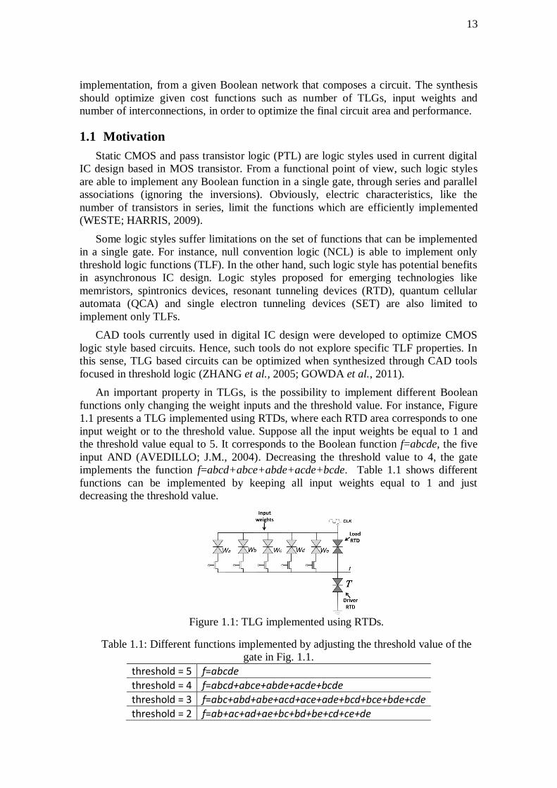