Nutrient Pollution and Eutrophication. Eutrophication Lecture Question –What is eutrophication?
Synthesis of SWMP Data for ASSETS Eutrophication Assessment of the North Atlantic Region NERR Systems
A Final Report Submitted to The NOAA/UNH Cooperative Institute for Coastal and Estuarine
Environmental Technology (CICEET)
Submitted by
Christopher Cayce Dalton1
Fred Dillon2
Dr. Suzanne Bricker3
Dr. Michele Dionne1
1Wells National Estuarine Research Reserve342 Laudholm Farm Road, Wells ME 04090
2FB Environmental97A Exchange Street, Suite 305, Portland ME 04101
3NOAA National Center for Coastal and Ocean Science 1305 East West Highway, Floor 8, Silver Spring MD 20910
November 30, 2006
This project was funded by a grant from NOAA/UNH Cooperative Institute for Coastal and Estuarine Environmental Technology, NOAA Grant Number #NA04NOS4190109

Wells National Estuarine Research Reserve2
Table of ContentsExpanded Executive Summary and Key Findings ...........................................................................4
Coastal Resource Issue: Eutrophication ...................................................................................4ASSETS is a Global Eutrophication Evaluation Tool ................................................................4Pressure-State-Response Framework ........................................................................................4Improvements Over Existing Tools .............................................................................................4Current Stage of Development: Integrating NERR-SWMP, MA-CZM Land Use Index ..........5ASSETS Characteristics .............................................................................................................5
Abstract .............................................................................................................................................7Introduction .......................................................................................................................................7
Introduction to ASSETS ..............................................................................................................7Introduction to SWMP ................................................................................................................8Application of ASSETS to SWMP ...............................................................................................9
Objectives ........................................................................................................................................11Study Period and Additional Data ...........................................................................................11
Methods ..........................................................................................................................................11Evolution of the NEEA-ASSETS Methodology .........................................................................11Influencing Factors ...................................................................................................................12Overall Eutrophic Condition ....................................................................................................14Future Outlook..........................................................................................................................18Overall Classification Grade ....................................................................................................18Land Use Index (LUI) ...............................................................................................................19
Results .............................................................................................................................................20Discussion .......................................................................................................................................22
Results of Assessment ...............................................................................................................22National and Regional Context ................................................................................................23Evaluating the Methodology and Integration with SWMP ......................................................24
Utilization .......................................................................................................................................26End User Application ...............................................................................................................26Knowledge Exchange ...............................................................................................................26Partnerships .............................................................................................................................27Next Steps to Application ..........................................................................................................27
References .......................................................................................................................................28Appendix I: Individual System Results .........................................................................................32Webhannet Estuary .........................................................................................................................32
Data Sources ............................................................................................................................32I. Susceptibility .........................................................................................................................32II. Influencing Factors (IF) .......................................................................................................33III. Overall Eutrophic Condition (OEC) ..................................................................................35IV. Future Outlook (FO) ...........................................................................................................38V. Overall Classification Grade (ASSETS) ...............................................................................39References .................................................................................................................................39
Merriland / Branch / Little River (MBLR) Estuary .......................................................................41Data Sources ............................................................................................................................41I. Susceptibility .........................................................................................................................41II. Influencing Factors (IF) .......................................................................................................42III. Overall Eutrophic Condition (OEC) ..................................................................................43IV. Future Outlook (FO) ...........................................................................................................45V. Overall Classification Grade (ASSETS) ...............................................................................46References .................................................................................................................................46
Great Bay Estuary...........................................................................................................................47Data Sources ............................................................................................................................47I. Susceptibility .........................................................................................................................47
Synthesis of SWMP and ASSETS for North Atlantic Region NERRs 3
II. Influencing Factors (IF) .......................................................................................................48III. Overall Eutrophic Condition (OEC) ..................................................................................51IV. Future Outlook (FO) ...........................................................................................................53V. Overall Classification Grade (ASSETS) ...............................................................................53References .................................................................................................................................53
Waquoit Bay Estuary ......................................................................................................................55Data Sources ............................................................................................................................55I. Susceptibility .........................................................................................................................55II. Influencing Factors (IF) .......................................................................................................56III. Overall Eutrophic Condition (OEC) ..................................................................................57IV. Future Outlook (FO) ...........................................................................................................61V. Overall Classification Grade (ASSETS) ...............................................................................62References .................................................................................................................................62
Narragansett Bay Estuary ...............................................................................................................64Data Sources ............................................................................................................................64I. Susceptibility .........................................................................................................................65II. Influencing Factors (IF) .......................................................................................................66III. Overall Eutrophic Condition (OEC) ..................................................................................67IV. Future Outlook (FO) ...........................................................................................................72V. Overall Classification Grade (ASSETS) ...............................................................................72References .................................................................................................................................72
Old Woman Creek ...........................................................................................................................74Data Sources ............................................................................................................................74I. Susceptibility .........................................................................................................................75II. Influencing Factors (IF) .......................................................................................................75III. Overall Eutrophic Condition (OEC) ..................................................................................76IV. Future Outlook (FO) ...........................................................................................................78V. Overall Classification Grade (ASSETS) ...............................................................................79References .................................................................................................................................80
Appendix II: Additional Land Use Index Information ..................................................................81Appendix III: Maps of ASSETS Component Results ...................................................................90
Wells National Estuarine Research Reserve4
Expanded Executive Summary and Key FindingsCoastal Resource Issue: EutrophicationThe Assessment of Estuarine Trophic Status (ASSETS) was developed to meet the need for an accurate, transferable and accessible method of measuring excessive nutrient enrich-ment (eutrophication) in estuaries and coastal waters. Legislative drivers include US Clean Water Act of 1972, US Harmful Algal Bloom and Hypoxia Research and Control Act of 1998 and the EU Water Framework Directive (2000/60/EC), EU UWWTD and Nitrates Directives – Definition of Sensitive Areas and Vulnerable Zones.
ASSETS is a Global Eutrophication Evaluation ToolASSETS builds on earlier efforts such as NOAA’s National Estuarine Eutrophication Survey from the early 1990’s and the National Estuarine Eutrophication Assessment (NEEA) from 1998 to the present. These earlier efforts relied heavily on expert opinion and heuristic analysis. ASSETS development is driven by a need for a more quantitative and accessible approach to evaluating eutrophication. No significant regulatory barriers to ASSETS devel-opment were encountered in this study.
ASSETS has been applied to 157 estuaries around the world. These results, detailed discus-sion of many case studies and continuing updates about ASSETS can be found at http://www.eutro.org. In addition, the website http://www.eutro.us hosts the latest NEEA survey update, containing results of the survey along with physical characteristics, hydrology, land use, population, climate, and sediment and nutrient loads for estuaries in the database.
Pressure-State-Response FrameworkThe method uses a pressure-state-response model with multiple parameters and an inclu-sive approach to data, summarized as follows:
Pressure: Influencing Factors (IF)Susceptibility of estuary (dilution and flushing)Nutrient loading
State: Overall Eutrophic Status (OEC)Primary symptoms: chlorophyll-a, macroalgaeSecondary symptoms: low dissolved oxygen, submerged aquatic veg-tation loss, hazardous/nuisance algal blooms
Response: Future Outlook (FO)Susceptibility of estuary (dilution and flushing)Nutrient loading trends
Improvements Over Existing ToolsASSETS adopted the above framework while streamlining and quantifying the NEEA methodology, using five symptoms from the original field of sixteen, and developing sta-tistical criteria whenever possible. Symptoms were divided into primary and secondary categories. Primary symptoms are ones that would be expected to manifest first when ex-cess nutrients become available to coastal waters, and include turbidity, high chlorophyll-a concentrations, and macroalgal blooms. Secondary symptoms are those expected when
•··
•··
•··
Synthesis of SWMP and ASSETS for North Atlantic Region NERRs 5
excessive nutrient inputs have persisted to the point where eutrophication has become en-trenched, including dissolved oxygen depletion, submerged aquatic vegetation loss, toxic algal blooms and changes in benthic and pelagic community composition. This study has identified the need for National Estuarine Research Reserves to include macroalgae in its System Wide Monitoring Program bio-monitoring build-out.
Current Stage of Development: Integrating NERR-SWMP, MA-CZM Land Use IndexSystem Wide Monitoring Program (SWMP) is an expanding component of the National Estuarine Research Reserve (NERR) system in the United States. There are 26 NERRs around the country, containing over one million acres of protected estuarine waters, wet-lands and adjacent uplands, and representing every known climatic zone in the nation and 15 biogeographic regions. The SWMP program has several characteristics valuable to the ASSETS framework, including excellent temporal coverage of data, thorough quality con-trol and uniform national protocols. Low spatial coverage is a limitation. The land use component of SWMP remains to be developed, and the current study demonstrates one possible approach to implementation.
ASSETS CharacteristicsCost: ASSETS uses existing data and basic desktop software. Costs are pri-marily labor, communications (data collection was greatly improved by on-site visits). ArcGIS software was used for the Land Use Index component.
Maintenance requirements: ASSETS requires no maintenance beyond data archival. However, it is intended for replication at 3 to 10 year intervals in or-der to observe trends and evaluate the predictive ability of past applications.
Accuracy: Available data should be evaluated for accuracy before being used in ASSETS. The results provided by ASSETS are intended to be ac-cessible to managers and non-scientists, while the evaluation process creates a telescoping level of detail for each parameter and for each salinity zone. Those who seek more detail than an overall grade can find it.
Speed: ASSETS is intended as a rapid and accessible evaluation tool. Data collection requires significant time. Application of ASSETS requires ma-nipulation of spreadsheet or database software. Once all data is collected, is it estimated that it would take two weeks to apply ASSETS to one estuary.
Ease of use: A step-by-step method has been submitted with this report. Skills in spreadsheet or database software for basic statistical manipulation (percentiles, means, medians) is required. If land use coverage is not avail-able for the lands adjacent to the estuary under study, then GIS software and land use categorization skills will be required.
End user capacity requirements: Data requirements include estuarine hy-drology (volume, freshwater inflow, tidal range, degree of stratification),
•
•
•
•
•
•
Wells National Estuarine Research Reserve6
monitoring data (dissolved oxygen, chlorophyll-a, hazardous/nuisance algal blooms, submerged aquatic vegetation, macroalgae), nutrient loading data for estuary, or a nutrient monitoring program (dissolved inorganic nitrogen or total nitrogen), trends in population, wastewater treatment, agriculture and other sources of nutrients. ArcGIS software (or equivalent) is necessary to apply the Land Use Index.
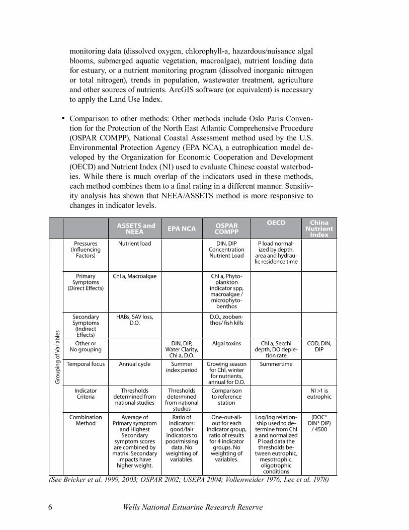
Comparison to other methods: Other methods include Oslo Paris Conven-tion for the Protection of the North East Atlantic Comprehensive Procedure (OSPAR COMPP), National Coastal Assessment method used by the U.S. Environmental Protection Agency (EPA NCA), a eutrophication model de-veloped by the Organization for Economic Cooperation and Development (OECD) and Nutrient Index (NI) used to evaluate Chinese coastal waterbod-ies. While there is much overlap of the indicators used in these methods, each method combines them to a final rating in a different manner. Sensitiv-ity analysis has shown that NEEA/ASSETS method is more responsive to changes in indicator levels.
•
ASSETS and
NEEA EPA NCA OSPAR COMPP
OECD China Nutrient
Index
Gro
upin
g of
Var
iabl
es
Pressures (Influencing
Factors)
Nutrient load DIN, DIP ConcentrationNutrient Load
P load normal-ized by depth,
area and hydrau-lic residence time
Primary Symptoms
(Direct Effects)
Chl a, Macroalgae Chl a, Phyto-plankton
indicator spp, macroalgae / microphyto-
benthos
Secondary Symptoms
(Indirect Effects)
HABs, SAV loss, D.O.
D.O., zooben-thos/ fish kills
Other or No grouping
DIN, DIP, Water Clarity,
Chl a, D.O.
Algal toxins Chl a, Secchi depth, DO deple-
tion rate
COD, DIN, DIP
Temporal focus Annual cycle Summer index period
Growing season for Chl, winter for nutrients,
annual for D.O.
Summertime
IndicatorCriteria
Thresholds determined from national studies
Thresholds determined
from national studies
Comparison to reference
station
NI >1 is eutrophic
Combination Method
Average of Primary symptom
and Highest Secondary
symptom scores are combined by
matrix. Secondary impacts have
higher weight.
Ratio of indicators: good/fair
indicators to poor/missing
data. No weighting of
variables.
One-out-all-out for each
indicator group, ratio of results for 4 indicator
groups. No weighting of
variables.
Log/log relation-ship used to de-termine from Chl a and normalized
P load data the thresholds be-
tween eutrophic, mesotrophic, oligotrophic conditions
(DOC* DIN* DIP)
/ 4500
(See Bricker et al. 1999, 2003; OSPAR 2002; USEPA 2004; Vollenweider 1976; Lee et al. 1978)
Synthesis of SWMP and ASSETS for North Atlantic Region NERRs 7
AbstractThe Assessment of Estuarine Trophic Status (ASSETS)—an accurate, transferable and ac-cessible method of measuring eutrophication in estuaries and coastal waters—was applied at 5 northeast National Estuarine Research Reserves (NERRs) in the United States. The study used 2002-2004 data from the NERR System Wide Monitoring Program (SWMP), which tracks short term variability and long term changes in estuarine parameters such as chlorophyll-a, dissolved oxygen and dissolved inorganic nitrogen. Objectives of the project included determining the level of eutrophication at the estuaries studied, improving the ASSETS methodology, exploring integration of ASSETS and SWMP, investigating the relationship between adjacent land use and eutrophic status.
The study found that in the northeast eutrophic conditions worsened north to south, going from the second and third highest grades at the two northernmost estuaries to the lowest possible grade in the three southernmost estuaries, which corresponds generally with a decrease in tidal range and an increase in population density. Lower intensities of develop-ment in adjacent land use surrounding the estuarine channel was generally found to corre-late with lower eutrophic conditions. However, land use surrounding the marsh system as a whole did not show such a correlation. Future conditions were expected to remain the same in one system (Narragansett Bay) due to planned improvements in wastewater treatment. In all other systems, conditions were expected to worsen.
IntroductionEutrophication of coastal waters in the United States is extensive, as shown by Bricker et al. (1999) in the National Estuarine Eutrophication Assessment (NEEA). An estimated 60% of our nation’s coastal waters suffer from excessive nutrient inputs, creating problems such as low dissolved oxygen which threatens the survival of fish, shellfish and benthic organisms; overgrowth of algae which can be unsightly, have negative effects on natural biota, and interfere with navigation and recreation; loss of seagrasses which provide habitat invalu-able to sustaining commercial and recreational fisheries; blooms of toxic or nuisance algae which cause restrictions in commercial fishing and may hamper recreational opportunities. NEEA and other studies (CENR 2003, Boesch 2001, NRC 2000) identify nutrient enrich-ment as one of the most significant threats to estuarine and coastal waters, and have urged that additional research and assessment be part of the management strategies to improving these conditions.
Introduction to ASSETSAssessment of Estuarine Trophic Status (ASSETS) was developed to meet the need for an accurate, transferable and accessible method of measuring eutrophication in estuaries and coastal waters. The method evolved from the National Estuarine Eutrophication Survey conducted by NOAA from 1992 to 1997 (NOAA 1996, 1997a, b, c, 1998) and the National Estuarine Eutrophication Assessment (NEEA) conducted from 1998 to the present, and oth-ers (Bricker et al. 1999, 2002, 2003, 2006). In these prior efforts, a pressure-state-response framework was developed to evaluate eutrophication of estuarine waters, summarized as follows:

Wells National Estuarine Research Reserve8
Pressure: Influencing Factors (IF)Susceptibility of estuary (dilution and flushing)Nutrient loading
State: Overall Eutrophic Condition (OEC)Symptoms of eutrophication (chlorophyll-a, oxygen depletion, etc).
Response: Future Outlook (FO)Susceptibility of estuary (dilution and flushing)Future nutrient loading predictions
Nutrient concentrations of estuarine waters were not included as a symptom of eutrophica-tion, since they represent the net result of physical, chemical and biological processes and may be high or low when eutrophication is clearly a problem. Instead, symptoms where divided into primary and secondary categories. Primary symptoms are those expected first when excess nutrients become available to coastal waters, such as turbidity, high chloro-phyll-a concentrations, and macroalgal blooms. Secondary symptoms are those expected when excessive nutrient inputs have persisted and eutrophication is entrenched, includ-ing dissolved oxygen depletion, submerged aquatic vegetation loss, toxic algal blooms and changes in benthic and pelagic community composition.
Legislation in the US and Europe has driven the development of several methods for as-sessing eutrophication. These laws include the US Clean Water Act of 1972, US Harmful Algal Bloom and Hypoxia Research and Control Act of 1998 and the EU Water Framework Directive (2000/60/EC), EU Urban Waste Water Treatment Directive (UWWTD) and Nitrates Directives – Definition of Sensitive Areas and Vulnerable Zones. Other methods besides NEEA/ASSETS using a suite of chemical and biological indicators to determine a single score for eutrophication include the National Coastal Assessment (US EPA 2004) and the Oslo Paris Convention for the Protection of the North Sea Comprehensive Procedure (OSPAR COMPP, OSPAR, 2001). Sensitivity analysis has shown that NEEA/ASSETS method is more responsive to changes in indicator levels (Ferreira et al. in press).
The website http://www.eutro.org contains further information about the ASSETS meth-odology, including results from 157 estuaries around the world, detailed case studies, and updates to ASSETS. The website http://www.eutro.us hosts the latest NEEA survey update, containing results of the survey along with physical characteristics, hydrology, land use, population, climate, and sediment and nutrient loads for estuaries in the database.
Introduction to SWMPSystem Wide Monitoring Program (SWMP) is an expanding component of the National Estuarine Research Reserve (NERR) system in the United States. Twenty six NERRs around the country contain over one million acres of protected estuarine waters, wetlands and adjacent uplands, and represent every known climatic zone in the nation and 15 bio-geographic regions. SWMP was established in 1995 in order to track short term variability and long term changes in estuarine environments within the NERR system, and consists of three phased-in components: abiotic parameters, biological monitoring, and watershed and land use classification (Owen et al. 2005).
•··
•·
•··
Synthesis of SWMP and ASSETS for North Atlantic Region NERRs 9
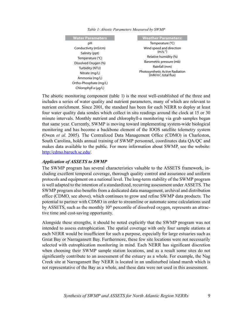
The abiotic monitoring component (table 1) is the most well-established of the three and includes a series of water quality and nutrient parameters, many of which are relevant to nutrient enrichment. Since 2001, the standard has been for each NERR to deploy at least four water quality data sondes which collect in situ readings around the clock at 15 or 30 minute intervals. Monthly nutrient and chlorophyll-a monitoring via grab samples began that same year. Currently, SWMP is moving toward implementing system-wide biological monitoring and has become a backbone element of the IOOS satellite telemetry system (Owen et al. 2005). The Centralized Data Management Office (CDMO) in Charleston, South Carolina, holds annual training of SWMP personnel, coordinates data QA/QC and makes data available to the public. For more information about SWMP, see the website: http://cdmo.baruch.sc.edu/.
Application of ASSETS to SWMPThe SWMP program has several characteristics valuable to the ASSETS framework, in-cluding excellent temporal coverage, thorough quality control and assurance and uniform protocols and equipment on a national level. The long-term stability of the SWMP program is well adapted to the intention of a standardized, recurring assessment under ASSETS. The SWMP program also benefits from a dedicated data management, archival and distribution office (CDMO, see above), which continues to grow and refine SWMP data products. The potential to partner with CDMO in order to streamline or automate some calculations used by ASSETS, such as the monthly 10th percentile of dissolved oxygen, represents an attrac-tive time and cost-saving opportunity.
Alongside these strengths, it should be noted explicitly that the SWMP program was not intended to assess eutrophication. The spatial coverage with only four sample stations at each NERR would be insufficient for such a purpose, especially for large estuaries such as Great Bay or Narragansett Bay. Furthermore, these few site locations were not necessarily selected with eutrophication monitoring in mind. Each NERR has significant discretion when choosing their SWMP sample station locations, and as a result some sites do not significantly contribute to an assessment of the estuary as a whole. For example, the Nag Creek site at Narragansett Bay NERR is located in an undisturbed island marsh which is not representative of the Bay as a whole, and these data were not used in this assessment.
Table 1: Abiotic Parameters Measured by SWMP
Water ParameterspH
Conductivity (mS/cm)Salinity (ppt)
Temperature (°C)Dissolved Oxygen (%)
Turbidity (NTU)Nitrate (mg/L)
Ammonia (mg/L)Ortho-Phosphate (mg/L)
Chlorophyll a (µg/L)
Weather Parameters:Temperature (°C)
Wind speed and direction (m/s; °)
Relative humidity (%)Barometric pressure (mb)
Rainfall (mm)Photosynthetic Active Radiation
(mM/m2, total flux)
Wells National Estuarine Research Reserve10
In two cases, the incomplete spatial coverage from the SWMP program was compensated by other monitoring programs which use the same or similar equipment. In Narragansett Bay, the Bay Window program is a cooperative network of buoy and dock mounted sondes offering an expanded coverage of the Bay. This program did not offer the same high stan-dard as SWMP in terms of data availability and metadata. However, it did show significant improvement from the start to end of the study period. While it showed limitations for these years, it is expected to be a good resource for the future. In Great Bay, the New Hampshire Department of Environmental Services (NHDES) and the Great Bay Estuary Partnership (GBEP) maintain sondes and a nutrient monitoring program that are very similar to SWMP and expand spatial coverage to nearly all parts of that system.
Volunteer water quality data was also used when available, keeping in mind possible limitations of these programs. While the Great Bay Coastal Watch program benefits from long-term trained volunteers and an EPA-approved Quality Assurance Project Plan, the Watershed Evaluation Team program at the Wells NERR is intended primarily as an edu-cational experience for junior and high school students. Some parameters, especially mac-roalgal blooms, did not benefit from formal monitoring programs at any NERR. In this case, a heuristic approach was taken, drawing on the expert knowledge of those who work within the estuary.
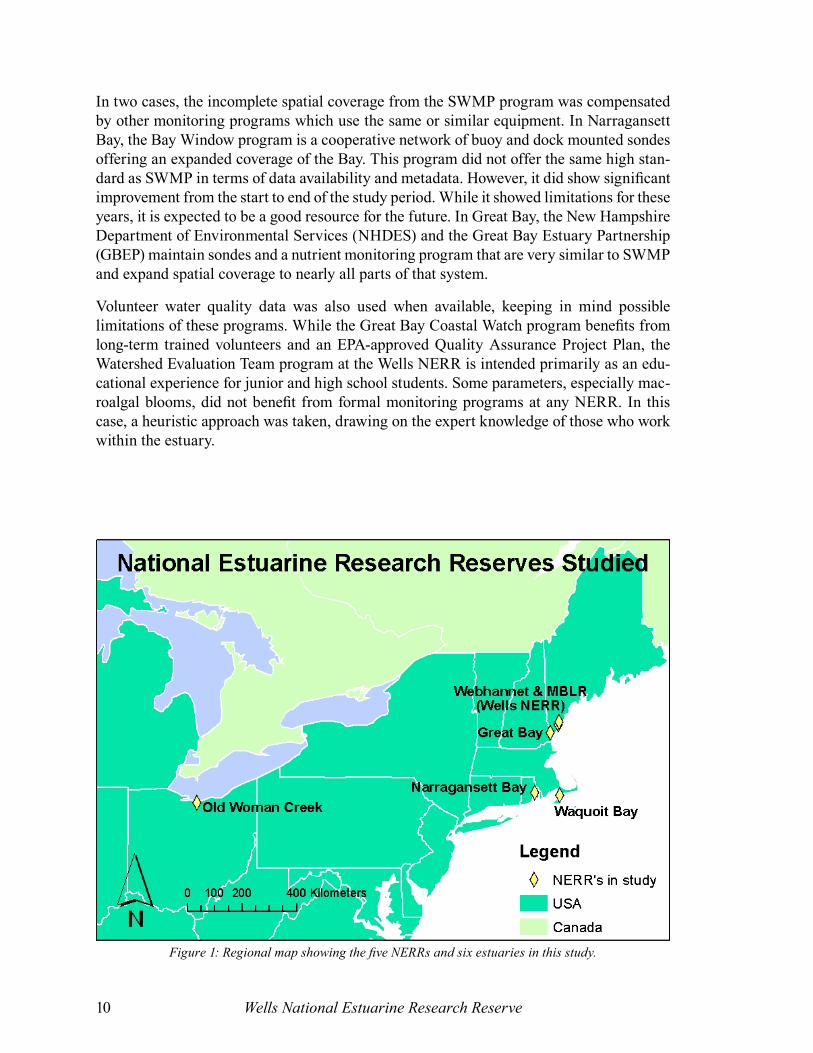
Figure 1: Regional map showing the five NERRs and six estuaries in this study.

Synthesis of SWMP and ASSETS for North Atlantic Region NERRs 11
ObjectivesSeveral goals were set forth for this application of ASSETS to northeast region NERRs (the five NERRs in this study are shown in Figure 1):
Determine the level of eutrophication at the NERRs chosen for study, along with identifying the likely sources and possible management responses. Improve the ASSETS methodology itself by exploring integration with SWMP and identifying possible areas for improvement. A two day work-shop at the Wells NERR in June 2006 helped meet this goal as participants from the study sites were brought together to review the draft results and provide feedback.Train regional scientists, policy makers and educators in the application of ASSETS.Inform stakeholders in the region of the results of this study, along with ap-propriate background on the methods used.Investigate the relationship between adjacent land use and eutrophic status as measured by ASSETS in the study area.
Study Period and Additional DataThe study period used in this report was 2002-2004, which corresponds to the first three years for which nutrient data is available under SWMP. In two cases (Wells NERR and Great Bay NERR), initial nutrient data was noted in the metadata as suspect and was omitted.
MethodsEvolution of the NEEA-ASSETS MethodologyASSETS grew out of the intention for more a streamlined, accessible and quantitative ap-plication of the NEEA approach. The ASSETS methodology as applied here was taken pri-marily from three recent publications, the NEEA report (Bricker et al. 1999), the Ecological Modelling paper which presented the Influencing Factors quantitative model of nutrient pressure (Bricker et al. 2003) and the Gulf of Maine Pilot Study (Bricker et al. 2006). Some results of the present report can be compared to those in the Gulf of Maine report, although Waquoit Bay, the Merriland/Branch/Little River (MBLR) Estuary and Old Woman Creek have not been previously studied by ASSETS. Waquoit Bay was, however, included in the 2006 NEEA update survey (Bricker et al. in press). Finally, the Human Use Indicator presented in the most recent study (Bricker et al. 2006) was beyond the scope of this project and is not applied here. In its place, a land use component, adopted from Massachusetts Coastal Zone Management Land Use Index method (Carlisle 2002, 2004) was applied in order to test the hypothesis that estuaries surrounded by more heavily developed land are correlated with higher eutrophication scores.
Most components of ASSETS have been maintained from previous studies: the basic Pressure-State-Response framework, the hierarchy of primary and secondary symptoms, weighting symptoms by three salinity zones within the estuary, the quantitative categories
•
•
•
•
•
Wells National Estuarine Research Reserve12
for symptoms, and the system of logical decision tables used to reach the final results. In Overall Eutrophic Condition (below), the rationale for each symptom was evaluated and modified to better match the temporal scale of available data. Additionally, the use of salin-ity zones was reinstated as in the two prior reports, after having been omitted in the 2006 Gulf of Maine study (Bricker et al. 2006). These salinity zones were refined as described below.
Influencing FactorsThe Pressure component under ASSETS is called Influencing Factors (IF) and is made up of three parts: dilution potential, flushing potentials and a nutrient loading score.
Dilution anD Flushing Potentials
Both dilution and flushing under ASSETS are determined quantitatively, through the use of a logical decision table. Dilution is based on just two inputs, vertical stratification and the volume of the estuary or its freshwater fraction. For a few estuaries in this study, it appears that the dilution potential is underestimated by the original IF decision tables due to the fact that these estuaries are very small when considered in a national context. In cases where the scientific literature clearly contradicted the ASSETS methodology (e.g., Webhannet Estuary), the literature result was adopted and ways to improve the accuracy of the methodology were sought. The units used for estuary volume in prior reports are not indicated in those reports, but are known to be cubic feet. For this reason, both cubic feet and cubic meters are provided here.
The ASSETS methods for determining flushing potential seemed more robust across the full size range of estuaries included in this study. Both tidal range and freshwater inflow are considered. However, it may need refinement for estuaries where the tidal range is nearly equal to the depth the estuary. This is the case for the Webhannet Estuary, where ASSETS determined flushing to be moderate. Literature describes flushing potential as high, due to the fact that the estuary almost empties out during low tide (Ward 2004). Units were not indicated in prior reports, but inflow units are known to be per day and are indicated here (volume units cancel when divided). Susceptibility was determined from dilution and flushing potential using the same decision table as in Bricker et al. (1999).
nutrient loaDing score
The original NEEA report relied upon USGS SPARROW (spatially referenced regressions of contaminant transport on watershed attributes; Smith et al. 1997) model to provide nutri-ent loading information in a nationally comparable format. Given that the underlying data for SPARROW is often outdated, the original NEEA report identified the need to better characterize the nutrient pressures on estuaries (Bricker et al. 1999).
The Influencing Factors model (originally called Overall Human Influence) was developed by Bricker et al. (2003) for this purpose and has been applied here. This simple model aims to quantify the ratio in the estuary of watershed source dissolved inorganic nitrogen (DIN) to total DIN (from combined offshore and watershed sources), with total nitrogen some-times being substituted for DIN. The higher the proportion of local source DIN, the higher the nutrient pressure on the estuary is considered to be. The model makes a few simplifying

Synthesis of SWMP and ASSETS for North Atlantic Region NERRs 13
assumptions: all nutrients in the estuary come either from the watershed via freshwater tributaries or from offshore (i.e., no loading directly from estuary banks, groundwater or atmosphere), and DIN is conserved in the estuary between the two sample stations. This method calculates this ratio from mean DIN measurements at two end members of the estuary—a sample station at the mouth used to represent offshore water and one at the head of tide to represent incoming freshwater—and a dilution model based on an average salinity within the estuary.
At some NERRs, sample station locations were not well-suited to the underlying assump-tions of the above model. For example, there were multiple freshwater tributaries entering the estuary, or one or both end-member sample stations were missing due to sample stations being more centrally located in the estuary. In addition, the concept of an average salinity within the estuary appeared to be unnecessary, since the salinity of each SWMP nutrient sample is known or can be closely estimated based on sonde data, meaning actual dilution of marine water to freshwater could be determined for each sample. The basic quantitative model is:
Influencing Factors Nutrient Loading Formula = mh / (mb + mh) where: mh = DIN concentration from freshwater inflow end-member mb = DIN concentration from offshore end-member
These two components are defined by: mh = min * (So – Se)/So mb = msea * Se/Sowhere: min = DIN concentration (mg/L) in inflow to the estuary So = Salinity of ocean (ppt) Se = Average salinity of estuary (ppt) msea = DIN concentration (mg/L) of the ocean
alternate inFluencing Factors Formula ProPoseD
An alternative approach which makes fuller use of the data collected by SWMP is pro-posed here. It uses the same basic ratio as the ASSETS Influencing Factors calculation above: the ratio of watershed source DIN to combined watershed and offshore source DIN in order to measure nutrient pressure on the estuary. Instead of relying on two end member measurements, it considers each nutrient sample to occur in a linear relationship along the dilution gradient between freshwater inflow and offshore, full salinity water. This method, like the prior model, assumes all DIN in the estuary comes from either the watershed via freshwater sources (zero salinity) or from offshore sources (local marine salinity) and is conserved in the estuary. Instead of using an average salinity for the entire estuary as in ASSETS, however, this method uses the measured mean salinity of actual samples at each station.
The average salinity at two sample stations are plotted against the average DIN concentra-tion. Assuming DIN is conserved in the estuary and the only two sources are freshwater

Wells National Estuarine Research Reserve14
inflow and offshore water, salinity and DIN will vary in a linear relationship between these two end members as FW inflow become progressively more diluted by offshore water. This linear relationship is revealed by the two samle stations and it predicts the average DIN concentration at each of the two end members (Figure 2). If additional sample sta-tions are plotted on the graph, the assumption of conservation of DIN may itself be tested. Unfortunately, the placement of SWMP sample stations at the estuaries studied was not conducive to testing this assumption since they were typically in completely different tribu-taries and thus could not be considered on a path between the two sample stations used.
Final inFluencing Factors (iF) score
The decision table from Bricker et al. (2006) was used to determine the IF score from susceptiblity and the nutrient loading score using both the original and alternative methods for nutrient loading described above.
Overall Eutrophic ConditionThe Overall Eutrophic Condition component of NEEA considered 16 parameters, which were streamlined into six and divided into primary and secondary categories based on whether they are considered early or advanced indicators of eutrophication (Bricker et al. 1999). The most recent ASSETS study further narrowed these categories to five (Bricker et al. 2006), which are the same as those used here. The two primary symptoms are chloro-phyll-a (chl-a) and macroalgae. The three secondary symptoms are dissolved oxygen (DO), submerged aquatic vegetation loss (SAV), and hazardous/nuisance algal blooms (HAB).
Figure 2. The Influencing Factors nutrient loading model was refined to take advantage of measured salini-ties, instead of estimates of the idealized “average estuarine salinity” used in prior ASSETS studies.
Synthesis of SWMP and ASSETS for North Atlantic Region NERRs 15
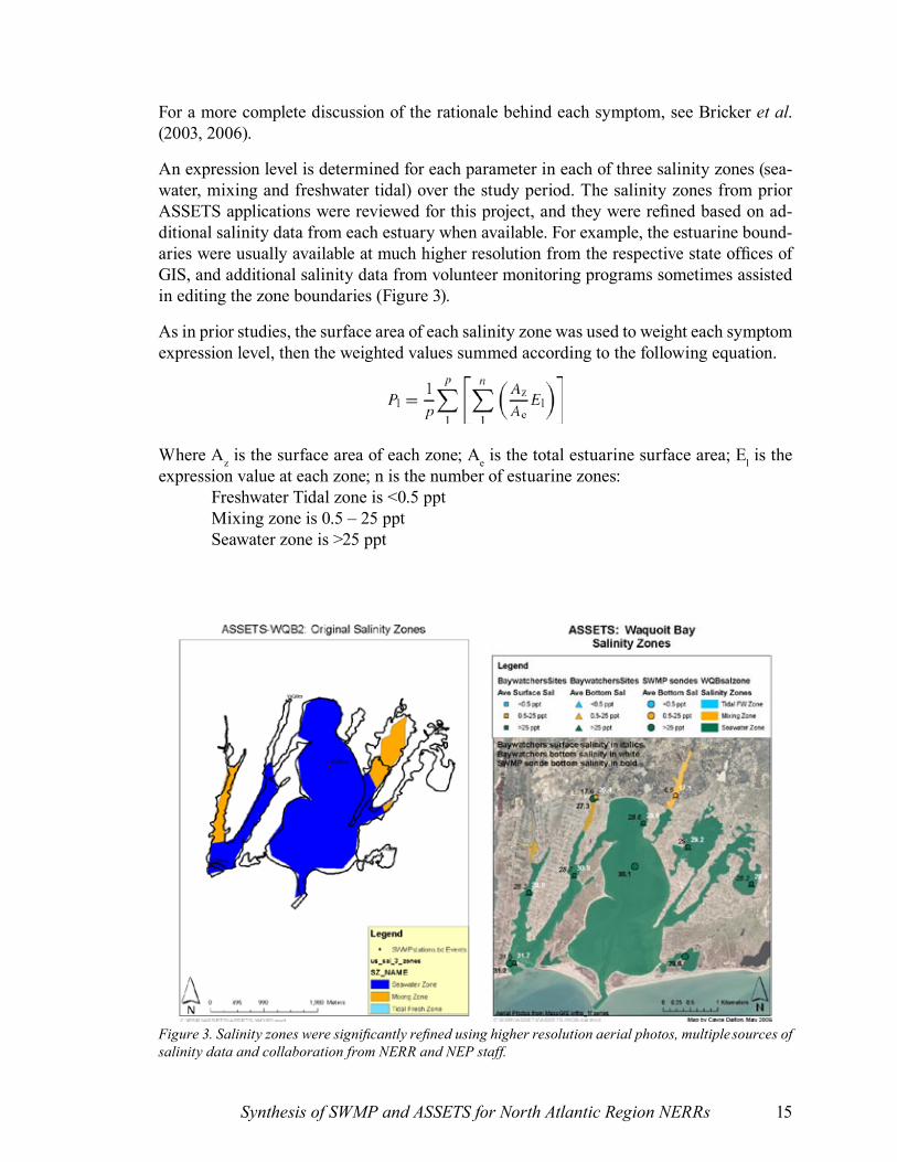
Figure 3. Salinity zones were significantly refined using higher resolution aerial photos, multiple sources of salinity data and collaboration from NERR and NEP staff.
For a more complete discussion of the rationale behind each symptom, see Bricker et al. (2003, 2006).
An expression level is determined for each parameter in each of three salinity zones (sea-water, mixing and freshwater tidal) over the study period. The salinity zones from prior ASSETS applications were reviewed for this project, and they were refined based on ad-ditional salinity data from each estuary when available. For example, the estuarine bound-aries were usually available at much higher resolution from the respective state offices of GIS, and additional salinity data from volunteer monitoring programs sometimes assisted in editing the zone boundaries (Figure 3).
As in prior studies, the surface area of each salinity zone was used to weight each symptom expression level, then the weighted values summed according to the following equation.
Where Az is the surface area of each zone; Ae is the total estuarine surface area; El is the expression value at each zone; n is the number of estuarine zones:
Freshwater Tidal zone is <0.5 pptMixing zone is 0.5 – 25 pptSeawater zone is >25 ppt

Wells National Estuarine Research Reserve16
The expression level for each symptom in each salinity zone is determined by a step-wise logical process that generally considers three factors: the concentration or level of occur-rence, the spatial coverage in the salinity zone, and the temporal frequency on a multi-year basis. When possible, these three components are quantified. Alternatively, a heuristic ap-proach is used. After aggregating each symptom across salinity zones, a numerical score is obtained between 0 and 1, which is then converted to a category (high, moderate, low). For all symptoms, spatial coverage is considered as a percentage of the salinity zone:
High (>50, ≤100%)Medium (>25, ≤50% )Low (>10, ≤25%)Very Low (>0, ≤10% )
Temporal frequency is considered on a multi-year basis:Episodic (conditions occur randomly, not necessarily every year)Periodic (conditions occur annually or predictably)Persistent (conditions occur continually throughout the year)
chloroPhyll-a
Yearly 90th percentiles were used to determine concentration level for each salinity zone. The same surface concentrations were used as in prior NEEA/ASSETS applications (Bricker et al. 1999):
Hypereutrophic: > 60 μg/LHigh: > 20, ≤ 60 μg/LMedium: > 5, ≤ 20 μg/LLow: > 0, ≤ 5 μg/L
macroalgae
Macroalgae have been the least monitored of the five eutrophication symptoms in ASSETS. The seemingly random spatial and temporal distribution of macroalgal mats complicates quantitative monitoring (Brawley 2002). Nonetheless, they are an important, and in some systems dominant, indicator of eutrophication. They bloom in estuaries with short resi-dence times of a few days whereas phytoplankton (and thus chlorophyll-a) respond more strongly when residence times are on the order of weeks or months (Valiela 2002). The need for further macroalgae monitoring was widely recognized among those who assisted with this study.
The use of stable isotopes of nitrogen in macroalgae has proven an effective predictor of ni-trogen loading (modeled) and DIN concentrations in tributaries to estuaries (Carmichael et al. 2004). This technique uses the different atomic signature of wastewater-source nitrogen from atmospheric/fertilizer nitrogen, which then shows up in algal tissues (which uptake nutrients directly from the water column). This technique has the potential to transform macroalgal blooms from a symptom of eutrophication to a source indicator. Cole et al. (2004) used this technique to successfully predict the percent of nitrogen in the water column from wastewater sources in Narragansett Bay, Waquoit Bay, and others. Nitrogen stable isotopes in phytoplankton chlorophyll has also been investigated (Sachs et al. 1999).
Synthesis of SWMP and ASSETS for North Atlantic Region NERRs 17
Isotopic analysis may be beyond the scope of SWMP and other basic monitoring programs, and not necessarily well-adapted to ASSETS if the intention is a simple and rapid overview of eutrophication. However, when studies of this type are available and resources permit, they could be incorporated into the pressure component since they provide key information about nutrient sources, potentially utilizing either the chl-a or macroalgae symptoms in ASSETS.
Macroalgae were assessed heuristically, since virtually no quantitative monitoring (and certainly no systematic monitoring) is currently conducted on a regional or national basis. The categories for macroalgae levels are simply problem (significant impact upon biological resources) or no problem (no significant impact). Biases in interpretations are acknowledged as a potential weakness in ASSETS, and further development of the indicator is planned.
DissolveD oxygen
The same categories of DO bottom concentrations were used as in prior NEEA/ASSETS applications with one modification for anoxia. The YSI dissolved oxygen probes used in SWMP has a reported accuracy of +/- 0.2 mg/L in the hypoxic and anoxic range. Therefore, a 10th percentile level of 0.2 mg/L was considered anoxic (YSI ca. 2002).
Anoxia: 0 mg/L (≤ 0.2 mg/L measured)Hypoxia: > 0.2 mg/L, ≤ 2 mg/LBiological Stress: >2mg/L, ≤ 5mg/LNo Problem: > 5mg/L
The 10th percentile was assessed on a monthly basis, not yearly as in prior ASSETS ap-plications. The high temporal resolution of the SWMP DO dataset (30 minute interval, or approximately 1440 readings/month/station when logger deployed nonstop) means a 10th percentile represents about 72 hours per month, consistent with the underlying concept that “low values of dissolved oxygen should be representative of system conditions, and not a single minimum value” (Bricker et al. 2003). This also resolved potential inconsisten-cies in seasonal deployment. Some non-SWMP sondes were deployed only for three or four summer months, others for six months, and most SWMP sondes for the entire year. Whether sondes are deployed for 4 summer months or year round, as long as deployments are during the months in which the lowest DO concentrations are likely to occur, the data are comparable. The frequency and distribution through time of the lowest 10th percentile category was used to determined temporal frequency.
In cases where a non-SWMP DO datasets provided too few data points per year to use a yearly percentile at each station, data were grouped by salinity zone and/or by multi-year sample period in order to obtain a minimum of about 30 samples. These changes are noted in each individual estuary results section in the appendix.
submergeD aquatic vegetation (sav) loss
The analysis of Submerged Aquatic Vegetation under ASSETS is a straightforward percent cover loss (or gain), with categories as follows:
Wells National Estuarine Research Reserve18
Trend:IncreaseDecreaseNo change
Magnitude of loss: High (>50%, ≤100%)Medium (>25%, ≤50%)Low (>0%, ≤25%)
The analysis of Submerged Aquatic Vegetation Loss under ASSETS shows room for re-finement. For example, many estuaries have suffered catastrophic losses in past decades, from which they have never recovered. Using the current methodology, ASSETS does not capture this history. In addition, if only remnants of prior beds exist, a very small change in acreage may show up as a very large percentage change, possibly skewing results. Just as importantly, shoot density and biomass changes should be considered when assessing submerged aquatic vegetation changes, not simply area covered. As an example of several of these issues, Great Bay eelgrass beds have suffered a large loss in biomass over the ten years ending in 2003, although the ASSETS methodology indicates only a “low” score (i.e., not a serious problem) for this symptom.
Fred Short (pers. comm.) suggested also that SAV loss could be considered a primary symptom of eutrophication, rather than a secondary symptom, citing observations that first eelgrass beds die off and then dissolved oxygen problems appear. Trowbridge (2006) sug-gested that increasing macroalgae is a plausible cause for the recent decline in eelgrass that has been observed in Great Bay, so that perhaps SAV loss may be considered an intermedi-ate symptom (showing up after an increase in macroalgae and before a drop in DO).
hazarDous/nuisance algal blooms (hab)Like macroalgae, HAB were evaluated heuristically. HAB’s were considered in relation-ship to their impact on biological resources, with the two categories being “problem,” and “no problem.” Duration, frequency and species composition are also considered. If HAB’s begin offshore and advecte into the estuary, ASSETS assigns a low score since estuarine nutrients were potentially sustaining, but not generating, the bloom. In none of the estuaries studied were HAB’s considered a problem, so this symptom was not evaluated in detail for this study.
Future OutlookThis component mirrors susceptibility, substituting future nutrient loading for current nu-trient loading. Population, land use, wastewater and other trends are examined to determine if nutrient loading to the estuary is expected to increase, decrease or remain unchanged. A decision table is then used which considers this trend with the susceptibility determined above to indicate the Future Outlook score.
Overall Classification GradeAfter determining numerical scores for the above three components, they are compared to a decision matrix which correlates them to an overall ASSETS score for the estuary. The decision matrix was not modified from previous applications of ASSETS.

Synthesis of SWMP and ASSETS for North Atlantic Region NERRs 19
Land Use Index (LUI)To investigate the potential relationship between coastal land uses and eutrophication lev-els, a simple land use analysis was conducted for each NERR using a modification of a method developed by the Massachusetts Office of Coastal Zone Management (Carlisle 2002, 2004). The Land Use Index (LUI) method is used for wetland assessment projects to quantify potential human-induced impacts from physical disturbances in the surrounding landscape. While it has since been refined considerably (MA-CZM, 2005), the LUI method still basically assumes that as the types and intensities of adjacent land uses increase, aquatic resources become more susceptible to cumulative impacts due to corresponding changes in hydrology, nutrient and sediment regimes and habitat quality. After applying the LUI method to a variety of coastal wetlands, MA-CZM found that the results provided a robust indicator of relative human disturbance from proximate land uses and activities while also allowing for the prioritization of wetland management strategies.
lui methoDology
The LUI method begins by delineating the extent of a given wetland study area and then establishes a 150 meter buffer or “zone of influence” around it. Land use types within the buffer area are then identified, either from existing land cover data (if available) or manu-ally using high resolution aerial photos. The land use classification scheme groups specific land use types into 7 more generalized categories (Table 2). This allows the LUI method to be adapted for a wide variety of different classification schemes.
Land Use Category Land Use Index CoefficientNatural Condition 0.95
Residential Low 0.66Agricultural 0.83
Urban 0.23Maintained Open 0.83Disturbed Open 0.86Residential High 0.25
Residential Medium 0.45
Table 2: MA-CZM land use classification system used in this study (MA-CZM, 2005)
These generalized land use categories are assigned LUI coefficients that describe the rela-tive disturbance level of each. More intensive land uses, such as large commercial centers and urban areas, are assumed to produce more pollutants and are therefore are more likely to adversely impact nearby aquatic resources than less intensive land uses, such as low density residential development. The steps of the method are outlined here:
Prepare Base MapIdentify, delineate, map wetland study site (if applicable)Identify, classify, and map surrounding land usesEstablish and map buffer zones (zones of influence)Compute area of buffer zonesCompute area of each unique land use in bufferApply Land Use Coefficients
•••••••

Wells National Estuarine Research Reserve20
Complete field-based Rapid Assessment FormCombine scores to generate the Land Use Index
All of these steps except for the rapid field assessment were used for the ASSETS-SWMP Data Synthesis Project. Field assessments were not conducted due to time and budget con-straints, particularly since the 2005 version of the LUI method includes an even more extensive field assessment component.
aPPlying lui to nerrs sites
In using the LUI method to estimate potential land use impacts to the NERR sites in our study, we essentially followed the methodology as outlined above (excluding field assess-ment), but instead of delineating a wetland study site we used the salinity zones to define the extent of our study areas. This worked well in most cases, where the estuarine channel was essentially equal to the channel plus surrounding marshes. However, for the MBLR and Webhannet, the surrounding vegetated marsh is large relative to the channel. In these cases, we could not use the salinity zone coverage (i.e., the channel) to represent the wet-land as a whole. In these cases, we calculated a LUI for both the estuarine channel and for the wetland as a whole, generating two separate scores.
ResultsA summary of results is presented in Tables 3-9 and Figure 4. For details on each system, see Appendix 1.
table 3: Webhannet estuary
Indices Methods Parameters/ Values Index category
ASSETS grade
PressureIF index
Susceptibility Dilution potential High Low Susceptibility Low
IF = 5
OEC = 5
FO = 1
Good
Flushing potential HighNutrient inputs Moderate
StateOEC index
PrimarySymptom
Chlorophyll a Low Low
LowMacroalgae No prob.
SecondarySymptom
Dissolved oxygen LowLowSAV Low
HAB No prob.ResponseFO index
Future nutri-ent pressures Steadily increasing development & population Worsen
High
••

Synthesis of SWMP and ASSETS for North Atlantic Region NERRs 21
table 4: mblr estuary
Indices Methods Parameters/ Values Index category
ASSETS grade
PressureIF index
Susceptibility Dilution potential Low Moderate Susceptibility Moderate
IF = 3
OEC = 5
FO = 1
Moderate
Flushing potential HighNutrient inputs Moderate
StateOEC index
PrimarySymptom
Chlorophyll a Low Low
LowMacroalgae No prob.
SecondarySymptom
Dissolved oxygen LowLowSAV Low
HAB No prob.ResponseFO index
Future nutri-ent pressures Steadily increasing development & population Worsen
High
table 5: great bay
Indices Methods Parameters/ Values Index category
ASSETS grade
PressureIF index
Susceptibility Dilution potential Low Moderate Susceptibility Moderate
HighIF = 3
OEC = 3
FO = 1
Poor
Flushing potential HighNutrient inputs Moderate High
StateOEC index
PrimarySymptom
Chlorophyll a High High
ModerateMacroalgae High
SecondarySymptom
Dissolved oxygen LowLowSAV Low
HAB No prob.ResponseFO index
Future nutri-ent pressures Increasing population Worsen
High
table 6: Waquoit bay
Indices Methods Parameters/ Values Index category
ASSETS grade
PressureIF index
Susceptibility Dilution potential Low Moderate Susceptibility Moderate
HighIF = 2
OEC = 1
FO = 1
Bad
Flushing potential HighNutrient inputs High
StateOEC index
PrimarySymptom
Chlorophyll a Moderate High
HighMacroalgae High
SecondarySymptom
Dissolved oxygen HighHighSAV Moderate
HAB No prob.ResponseFO index
Future nutri-ent pressures Increasing housing density and population Worsen
High
Wells National Estuarine Research Reserve22
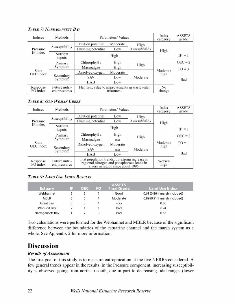
table 7: narragansett bay
Indices Methods Parameters/ Values Index category
ASSETS grade
PressureIF index
Susceptibility Dilution potential Moderate High Susceptibility High
IF = 1
OEC = 2
FO = 3
Bad
Flushing potential LowNutrient inputs High
StateOEC index
PrimarySymptom
Chlorophyll a High HighModerate
high
Macroalgae High
SecondarySymptom
Dissolved oxygen ModerateModerateSAV Low
HAB LowResponseFO index
Future nutri-ent pressures
Flat trends due to improvements in wastewater treatment
No change
table 8: olD Woman creek
Indices Methods Parameters/ Values Index category
ASSETS grade
PressureIF index
Susceptibility Dilution potential Low High Susceptibility High
IF = 1
OEC = 2
FO = 1
Bad
Flushing potential LowNutrient inputs High
StateOEC index
PrimarySymptom
Chlorophyll a High HighModerate
high
Macroalgae n/a
SecondarySymptom
Dissolved oxygen ModerateModerateSAV n/a
HAB Low
ResponseFO index
Future nutri-ent pressures
Flat population trends, but strong increase in regional nitrogen and phosphorous loads in
rivers in region since about 1995.Worsen
high
table 9: lanD use inDex results
DiscussionResults of AssessmentThe first goal of this study is to measure eutrophication at the five NERRs considered. A few general trends appear in the results. In the Pressure component, increasing susceptibil-ity is observed going from north to south, due in part to decreasing tidal ranges (lower
Estuary IF OEC FOASSETS
Final Grade Land Use IndexWebhannet 5 5 1 Good 0.61 (0.86 if marsh included)
MBLR 3 5 1 Moderate 0.89 (0.91 if marsh included)Great Bay 3 3 1 Poor 0.80
Waquoit Bay 2 1 1 Bad 0.74Narragansett Bay 1 2 3 Bad 0.63
Two calculations were performed for the Webhannet and MBLR because of the significant difference between the boundaries of the estuarine channel and the marsh system as a whole. See Appendix 2 for more information.

Synthesis of SWMP and ASSETS for North Atlantic Region NERRs 23
flushing). Under the State component, with regard to OEC there are no particular trends for individual symptoms expressed, but there is an overall trend toward worsening symptoms from north to south. Under Response, there is no clear trend, although the southernmost Atlantic estuary, Narragansett shows an improving outlook, while the northern estuaries all show conditions likely to worsen due to population increases. For a detailed assessment of each estuary, see Appendix 1.
National and Regional ContextPreliminary results of the recent update of the 1999 NEEA (http://www.eutro.us; Bricker et al. in press) shows that, nationally, there are still a significant number of US systems that are highly impacted by nutrient inputs in the early 2000s. Eutrophic conditions were mod-erate to high in 63 systems (57% of the total waterbody surface) and, as in the 1999 national assessment, estuaries with high levels of eutrophic conditions were found in every region. During the decade between studies, conditions in 35 systems improved and in 27 systems conditions have worsened. For some systems that have improved, Boston Harbor, Long Island Sound and Charlotte Harbor, it is the result of management measures that have been successful. However, even for the systems that have improved the future outlook is bleak with 44 of 141 systems expected to worsen in the future and only 15 expected to improve. We also know less now than we did a decade ago. The number of systems with inadequate data for assessment increased from 17 in the early 1990s to 43 in the early 2000s.
The results for the North Atlantic region in general are a contrast to results in other regions with less problems observed overall. However, there is a pattern of higher level problems
Figure 4. Final ASSETS grade, which synthesizes pressure-state-response into one score.
Wells National Estuarine Research Reserve24
in systems in the southern part of the region where population density is higher, land use is significantly less forested, and the tide range is lowest. The NEEA update and the ASSETS results here differ in some details (see Appendix 1), but this overall pattern is consistent. The future outlook for the region, where there were results, are bleak with 8 of the 11 systems reporting that conditions will worsen in the future. While these are systems in the southern part of the region, the bleak outlook should be a call to action to put into place management measures now that will prevent future degradation.
Evaluating the Methodology and Integration with SWMPThe second goal was to improve the ASSETS methodology, and explore its integration with SWMP. The need to refine certain aspects of ASSETS methodology is most clearly indicated when the criteria for a given component produce results that do not agree with known conditions. For example, the Webhannet Estuary was determined to have low dilu-tion potential under the ASSETS criteria, a result based on the estuary’s small dilution volume relative to other estuaries around the nation. However, Ward (2004) describes the estuary as exhibiting high dilution, citing freshwater inflow as only about 0.5% of the tidal prism. Similarly, flushing potential for the Webhannet was determined by the ASSETS de-cision table to be moderate, whereas the literate indicates the Webhannet is highly flushed. The Webhannet Estuary is at the far end of the spectrum of sites studied by ASSETS both in terms of its small size and large tidal range.
There are several possible approaches to adjusting the ASSETS criteria so that they accu-rately assess estuaries at the extreme end of the spectrum like the Webhannet. One method would be to modify the way flushing and/or dilution potentials are determined. Conceptually, dilution should include both solvent and solute, in this case the ratio of freshwater inflow to estuary volume (or the tidal prism in the case of a stratified water column). Currently, it only considers the solute: the volume of the estuary or its freshwater fraction.
Another strategy would be to create separate criteria for flushing and dilution based on estuarine typology. A similar issue was previously encountered in Florida Bay, where the ASSETS criteria for chlorophyll-a had to be tailored to local conditions in order to provide an accurate assessment of symptom expression (Ferreira et al. 2006, in press). A typol-ogy component is currently a high priority for development of the ASSETS methodology (Bricker, pers. comm.).
The state component of ASSETS also showed room for further refinement. First, the deci-sion table for dissolved oxygen should weight more heavily anoxia under low spatial or temporal frequency. In the case of Narragansett Bay, anoxia at low spatial distribution and episodic frequency under ASSETS would indicate that dissolved oxygen depletion is not a significant symptom of eutrophication in that estuary. The extensive fish kill in Greenwich Bay experienced during the study period, however, clearly paints a different picture. In this case, adjusting the scores that the decision table produce with a given combination of inputs may be an appropriate solution. Alternatively, ASSETS could be applied to subsections of a complex estuary such as Narragansett Bay, to better represent spatial variation in trophic condition.

Synthesis of SWMP and ASSETS for North Atlantic Region NERRs 25
Secondly, the SAV component should be considered. Fred Short (pers. comm.) suggested that SAV could be considered a primary symptom rather than a secondary, since in his view disappearing SAV precedes a decline in dissolved oxygen. Furthermore, the change in spatial coverage of eelgrass may not be the most meaningful metric to use. When a historically large eelgrass coverage has been reduced to a tiny remnant, any change in acreage will be large on a percent basis. More importantly, it does not consider changes in plant density which may be decreasing much faster than spatial extent, as is the case in Great Bay. While in this report, expert knowledge of changes in eelgrass status was read-ily available for comparison with the eelgrass results provided by ASSETS, ultimately the ASSETS methodology should generate as accurate a picture as possible using quantitative means alone.
A third challenge to the ASSETS methodology is the lack of a consistent monitoring pro-gram for macroalgae. It was beyond the scope of this study to implement such programs, and the fact that in some estuaries (Waquoit Bay) macroalgae is the single most dominant symptom of eutrophication, it was considered absolutely necessary to include macroalgae in the state component despite the heuristic nature of the evaluation.
The Influencing Factors component of ASSETS was easily refined to maximize the use of available data in the SWMP database, incorporating salinity measurements where a generalized model of salinity was used in prior studies. A likely weaknesses remains in the assumption of conservation of DIN in the estuary. This weakness can be overcome by the use of additional sampling stations which could be used to show whether DIN is in fact conserved. Other more sophisticated nutrient loading models are available, such as EPA Region 1 ArcView Generalized Watershed Loading Function which is specialized to the northeast, or the Gulf of Maine Watershed and Information Characterization System (GM-WICS), as well as more specific modeling efforts on a local basis. The much higher complexity of these models may preclude their use in ASSETS, for which user accessibility is a stated goal.
The third and fourth goals were to train researchers, policy makers and educators in the use of ASSETS, and to disseminate the picture of eutrophication it provides to these and other stakeholders. Results of a workshop with potential users and a step-by-step outline of the ASSETS methodology is presented below.
A final goal of this study was to investigate the relationship between adjacent land use and eutrophication as measured by ASSETS. When looking at the land use adjacent to the estuarine system as a whole (channels plus vegetated marsh), no clear relationship between the LUI and ASSETS scores was discernable (Table 9). In conducting the land use analysis, it became clear that the question of defining system boundaries could have significant im-plications. For three estuaries (Great Bay, Waquoit Bay and Narragansett Bay), at the reso-lution used for this project, the estuarine channel was essentially the same as the estuarine channel plus surrounding vegetated marsh, given that the channel was so much larger than the vegetated marsh. However, for the Webhannet and MBLR, this was not the case, and a separate analysis was performed that looked at land use adjacent to the channel itself. Using this definition, there does appear to be some correlation between adjacent land use and

Wells National Estuarine Research Reserve26
ASSETS score. Since ASSETS uses data which come exclusively from the water column, there may be some rationale for examining land use adjacent to the channel itself in relation to eutrophication scores. Perhaps in cases where land use adjacent to a marsh system is highly impacted but eutrophication is not observed in estuarine waters, that the vegetated marsh itself may be buffering the excessive nutrient enrichment, and may be itself suffering from some form of eutrophication. The further study of land use and eutrophication should make a distinction between estuarine waters and the vegetated marsh, perhaps conducting a separate land use analysis for each. See Appendix 1 for maps and figures.
UtilizationEnd User ApplicationThe ASSETS methodology was applied at five northeastern estuaries that are part of the NERR system, with the assistance and collaboration of the research directors at each NERR. Project staff were able to make site visits at the four New England reserves, while com-munication with Old Woman Creek was via e-mail and phone. At the two largest estuaries, Great Bay and Narragansett Bay, collaboration extended to state, quasi-governmental and non-profit organizations, as well. Details of these interactions are provided below.
Knowledge ExchangeProject staff visited the scientists at the four New England estuaries in late November and early December 2005. During these meetings, the ASSETS methodology was pre-sented to the research director of each NERR, Rhode Island Department of Environmental Management, and University of New Hampshire Jackson Estuarine Laboratory. During visits, the ASSETS methodology was presented and data were sought and discussed.
On June 12-13, the project staff held a workshop with researchers and educators from all of the estuaries (except Old Woman Creek) in which the methods were outlined, the draft results were presented and a discussion was held on how to best improve the ASSETS methodology. Below are highlights from this meeting.
Several comments focused on improving the technical aspects of the methodology, includ-ing better nutrient loading assessment, addition of a wetland analysis component, adop-tion of estuarine typologies and a statistical analysis to investigate predictive capacity. For example, a need to refine the loading component used in ASSETS was identified. The USGS SPARROW model is based on dated land use information, ranging from 1972 to 1992. Valiela’s N-LOAD model was mentioned as a possible candidate, as was the ArcView Generalized Watershed Loading Function under development by EPA Region 1. NOAA’s Coastal Services Center also provides a web-based nutrient loading tool (N-Spect, www.csc.noaa.gov/crs/cwq/nspect.html), although it focuses on nutrients in sediments.
ASSETS looks to water quality and aquatic communities for symptoms of eutrophica-tion. Jan Smith (Mass Bays and Islands National Estuary Program) suggested the wetlands themselves may also show signs of eutrophication which may not appear in highly flushed estuaries. With increasing development and impervious surface, the salinity zones may change, while the wetlands would remain stationary. The use of a wetland assessment tool (such as the one being developed by Massachusetts CZM) could accomplish this goal.
Synthesis of SWMP and ASSETS for North Atlantic Region NERRs 27
Estuarine typologies were mentioned as a way to refine the accuracy of the ASSETS quan-titative criteria across different types of systems. An example of this approach has already been initiated in Florida Bay, where the quantitative criteria for chlorophyll-a concentra-tions were localized since the original levels underestimated the severity of that parameter (Ferreira, 2006, in press). The ASSETS methodology is moving toward the implementation of this concept (Bricker, pers. comm.).
Finally, several participants mentioned the potential value of conducting a statistical evalu-ation of ASSETS results to determine the relationship between pressure and state, and to evaluate the predictive ability of ASSETS over the long term. This type of analysis could contribute to the further refinement of the methodology and ultimately augment its cred-ibility. If the predictive ability of ASSETS is demonstrated, then it would be possible to create ecological forecasts which may have a management value.
Linking ASSETS to positive management decisions was discussed. ASSETS was generally praised for its synthetic nature, and the ability to provide a quick general picture or ad-ditional levels of detail depending on the audience. The need for a regulatory driver and/or economic connection was identified. An ecological services concept, such as the continued application of a Human Use Indicator such as the one which examined recreational fish catch in relation to ASSETS, assigning an economic value to that catch (Bricker et al. 2003; Bricker et al. 2006), could in part fill this need. ASSETS may also be used to influ-ence future state regulations, which would link the results more closely to management decisions.
On June 15, 2006, project staff presented both on the ASSETS methodology and Great Bay’s results at the New Hampshire Estuaries Project Technical Advisory Committee meeting (see http://nhep.unh.edu/programs/nutrient.htm). This committee helps to establish Water Quality Standards in collaboration with NH DES and NHEP. Present at the meeting were representatives from EPA, University of New Hampshire, NH DES, Conservation Law Foundation and private consulting firms.
PartnershipsCollaborations were strengthened with many organizations through this study. Most notably, the System Wide Monitoring Program of the NERRs system, through the five northeast reserves, as described above. In addition, data was exchanged and methods were discussed with Great Bay Estuary Project, New Hampshire Department of Environmental Services, Great Bay Coastal Watch, Waquoit Bay Coast Watch, Rhode Island Department of Environmental Management, Narragansett Bay Commission, Heidelberg College and Massachusetts Coastal Zone Management.
Next Steps to ApplicationThe ASSETS methodology is readily accessible to coastal resources managers now through the step-by-step methodology submitted together with this report. This methodology brings together in one source several ASSETS papers and reports. Prior studies documenting the history of eutrophication at hundreds of estuaries both in the United States and abroad are available on the site http://eutro.org.
Wells National Estuarine Research Reserve28
ASSETS is undergoing additional development, so those interested in applying it should contact NOAA NCCOS (S. Bricker, principle investigator). Future developments will focus on an estuarine typology component, a human use/socioeconomic indicator to complet-ment the water quality index, refined nutrient loading, and the quantification of macroal-gae. Of these future plans, the macroalgal component is the one most in need of resources beyond those which are presently available to the developers of ASSETS. A standardized, quantitative method for monitoring macroalgae in relation to eutrophication is need that is acknowledged both by the developers of the ASSETS method and by the NERRs that were visited in this study.
Another next step would be the integration of the SWMP data stream with ASSETS. An important step in this process would be to evaluate the suitability of SWMP sample sta-tions for an assessment of eutrophication, as described above. The technical obstacles to this step involve authoring software which would access the SWMP database (available via web, or it could be integrated directly with the CDMO workflow), calculate the appropriate symptom level and return the associated ASSETS parameter to a eutrophication database. At the time of writing, CDMO has not yet moved to a SQL database, which has been a long term goal to facilitate working with the data. A one to two year project with a NERR-wide scope would be sufficient to evaluate the dissolved oxygen and chlorophyll-a and nutrient components of SWMP and author the appropriate software. Until this change has occurred, it would be premature to design software intended to access SWMP data.
ReferencesBoesch, D. 2002. Challenges and Opportunities for Science in Reducing Nutrient Over-enrichment of Coastal Ecosystems. Estuaries 25:744-758.
Brawley J.W. 2002. Dynamic Modeling of Nutrient Inputs and Ecosystem Responses in the Waquoit Bay Estuarine System. Dissertation, U. Maryland, College Park.
Bricker, S.B., C.G. Clement, D.E. Pirhalla, S.P. Orlando, and D.R.G. Farrow. 1999. National Estuarine Eutrophication Assessment. Effects of Nutrient Enrichment in the Nation’s Estuaries. NOAA, National Ocean Service, Special Projects Office and National Centers for Coastal Ocean Science, Silver Spring MD.
Bricker, S.B., J.G. Ferreira, and T. Simas. 2003. An Integrated Methodology for Assessment of Estuarine Trophic Status. Ecological Modelling 169: 39-60.
Bricker, S.B., D. Lipton, A. Mason, M. Dionne, D. Keeley, C. Krahforst, J. Latimer, J. Pennock. 2006. Improving methods and indicators for evaluating coastal water eutrophica-tion: a pilot study in the Gulf of Maine. Report to NOAA-CICEET. 66p.
Bricker, S.B., B. Dennison, B. Longstaff, J. Woerner, A. Jones, C. Wicks, K. Boicourt. National Estuarine Eutrophication Assessment: Effects of nutrient enrichment in the Nation’s estuaries 1999-2004. National Oceanic and Atmospheric Administration, National Ocean Service, National Centers for Coastal Ocean Science, Centers for Coastal Monitoring
Synthesis of SWMP and ASSETS for North Atlantic Region NERRs 29
and Assessment and The University of Maryland, Center for Environmental Science, Integration and Application Network. In press.
Bricker, S.B., G. Matlock, J. Snider, A. Mason, M. Alber, W. Boynton, D. Brock, G. Brush, D. Chestnut, U. Claussen, W. Dennison, E. Dettmann, D. Dunn, J. Ferreira, D. Flemer, P. Fong, J. Fourqurean, J. Hameedi, D. Hernandez, D. Hoover, D. Johnston, S. Jones, K. Kamer, R. Kelty, D. Keeley, R. Langan, J. Latimer, D. Lipton, R. Magnien, T. Malone, G. Morrison, J. Newton, J. Pennock, N. Rabalais, D. Scheurer, J. Sharp, D. Smith, S. Smith, P. Tester, R. Thom, D. Trueblood and R. Van Dolah. 2004. National Estuarine Eutrophication Assessment Update: Workshop summary and recommendations for development of a long-term monitoring and assessment program. Proceedings of a workshop 4-5 September 2002. Patuxent Wildlife Research Refuge, Laurel, Maryland.
Carlisle, B.K. 2002. Land Use Index: Wetland Evaluation Area Version: Description and Methodology 11/02. Massachusetts Coastal Zone Management, Wetland Assessment Program.
Carlisle, B.K., J.D. Baker, A.L. Hicks, J.P. Smith and A.L. Wilbur. 2004. Cape Cod Salt Marsh Assessment Project; Final Grant Report, Volume 1: Relationship of salt marsh indi-ces of Biotic Integrity to surrounding land use, 1999. Boston, MA. Massachusetts Office of Coastal Zone Management.
Carmichael, R.H., B. Annett, I. Valiela. 2004. Nitrogen Loading to Pleasant Bay, Cape Cod: Application of Models and Stable Isotopes to Detect Incipient Nutrient Enrichment of Estuaries. Marine Pollution Bulletin 48:137-143.
Cole, M.L., I. Valiela, K. D. Kroeger, G. L. Tomasky, J. Cebrian, C. Wigand, R. A. McKinney, S. P. Grady, M. H. Carvalho da Silva. 2004. Assessment of a d15N Isotopic Method to Indicate Anthropogenic Eutrophication in Aquatic Ecosystems. Journal of Environmental Quality. 33:124-132. Committee on Environmental and Natural Resources (CENR). 2000. Integrated assessment of hypoxia in the northern Gulf of Mexico. National Science and Technology Council, Committee on Environment and Natural Resources, Washington, DC.
Ferreira, J.G., S.B. Bricker, T.C. Simas, 2006. Application and sensitivity testing of an eutrophication assessment method on coastal systems in the United States and European Union. J. Environmental Management, In Press.
Holden, William F. 1997. Fresh Water, Suspended Sediment, and Nutrient Influx to the Little River and Webhannet River Estuaries, Wells, Maine. Dissertation, Boston University. 258 p.
Lee, G.F., W. Rast and R.A. Jones. 1978. Eutrophication of waterbodies: Insights for an age-old problem. Environmental Science & Technology 12:900-908.
National Oceanic and Atmospheric Administration (NOAA). 1996. NOAA’s Estuarine Eutrophication Survey. Volume 1: South Atlantic Region. National Oceanic and Atmospheric

Wells National Estuarine Research Reserve30
Administration, National Ocean Service, Office of Ocean Resources Conservation and Assessment. Silver Spring.
National Oceanic and Atmospheric Administration (NOAA). 1997a. NOAA’s Estuarine Eutrophication Survey. Volume 2: Mid-Atlantic Region. National Oceanic and Atmospheric Administration, National Ocean Service, Office of Ocean Resources Conservation and Assessment. Silver Spring.
National Oceanic and Atmospheric Administration (NOAA). 1997b. NOAA’s Estuarine Eutrophication Survey. Volume 3: North Atlantic Region. National Oceanic and Atmospheric Administration, National Ocean Service, Office of Ocean Resources Conservation and Assessment. Silver Spring.
National Oceanic and Atmospheric Administration (NOAA). 1997c. NOAA’s Estuarine Eutrophication Survey. Volume 4: Gulf of Mexico Region. National Oceanic and Atmospheric Administration, National Ocean Service, Office of Ocean Resources Conservation and Assessment. Silver Spring.
National Oceanic and Atmospheric Administration (NOAA). 1998. NOAA’s Estuarine Eutrophication Survey. Volume 5: Pacific Coast Region. National Oceanic and Atmospheric Administration, National Ocean Service, Office of Ocean Resources Conservation and Assessment. Silver Spring.
National Research Council (NRC). 2000. Clean Coastal Waters: Understanding and Reducing the Effects of Nutrient Pollution. National Academy of Sciences.
Oslo Paris Convention for the Protection of the North Sea (OSPAR). 2002. Common Assessment Criteria, their Assessment Levels and Area Classification within the Comprehensive Procedure of the Common Procedure. OSPAR Commission for the protec-tion of the marine environment of the North-East Atlantic. http://www.ospar.org/eng/html/welcome.html
OSPAR. 2001. Draft Common Assessment Criteria and their Application within the Comprehensive Procedure of the Common Procedure. Meeting of the eutrophication task group (ETG), London, 9-11 October 2001, ed. OSPAR convention for the protection of the marine environment of the North-East Atlantic. OSPAR Commission, London, England.
Owen, B., S. White. 2005. National Estuarine Research Reserve System 10 Anniversary Report on the System-wide Monitoring Program (SWMP) Data Applications: 1995 – 2005. NOAA Estuarine Reserves Division, Silver Spring MD. http://www.nerrs.noaa.gov/programs/SWMPReport.pdf
Sachs, J.P., D.J. Repeta, R. Goericke. 1999. Nitrogen and carbon isotopic ratios of chloro-phyll from marine phytoplankton. Geochimica et Cosmochimica Acta 63:1431-1441.
Smith, R.A., G.E. Schwarz and R.B. Alexander. 1997. Spatially referenced regressions on watershed attributes (SPARROW). Regional interpretation of water quality monitoring data. Water Resources Research 33: 2781-2798.
Synthesis of SWMP and ASSETS for North Atlantic Region NERRs 31
Trowbridge, P. March 2006. Environmental Indicator Report: Critical Habitats and Species. New Hampshire Estuaries Project, University of New Hampshire, Durham, NH.
United States Environmental Protection Agency (US EPA). December 2004. National Coastal Condition Report II. Office of Research and Development, Office of Water, Washington, DC. EPA-620/R-03/002. http://www.epa.gov/owow/oceans/nccr2/
Valiela, I., J.L. Bowen. 2002. Nitrogen Sources to Watershed and Estuaries: Role of Land Cove Mosaics and Losses within Watersheds. Environmental Pollution 118:239-248.
Vollenweider, R.A. 1976. Advances in defining critical loading levels for phosphorus in lake eutrophication. Mem Ist. Ital. Idrobio. 33: 53-83.
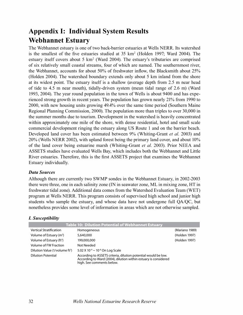
Wells National Estuarine Research Reserve32
Appendix I: Individual System ResultsWebhannet EstuaryThe Webhannet estuary is one of two back-barrier estuaries at Wells NERR. Its watershed is the smallest of the five estuaries studied at 35 km2 (Holden 1997; Ward 2004). The estuary itself covers about 5 km2 (Ward 2004). The estuary’s tributaries are comprised of six relatively small coastal streams, four of which are named. The southernmost river, the Webhannet, accounts for about 50% of freshwater inflow, the Blacksmith about 25% (Holden 2004). The watershed boundary extends only about 5 km inland from the shore at its widest point. The estuary itself is a shallow (average depth from 2.5 m near head of tide to 4.5 m near mouth), tidally-driven system (mean tidal range of 2.6 m) (Ward 1993, 2004). The year round population in the town of Wells is about 9400 and has expe-rienced strong growth in recent years. The population has grown nearly 21% from 1990 to 2000, with new housing units growing 49.4% over the same time period (Southern Maine Regional Planning Commission, 2000). The population more than triples to over 30,000 in the summer months due to tourism. Development in the watershed is heavily concentrated within approximately one mile of the shore, with dense residential, hotel and small scale commercial development ringing the estuary along US Route 1 and on the barrier beach. Developed land cover has been estimated between 9% (Whiting-Grant et al. 2003) and 20% (Wells NERR 2002), with upland forest being the primary land cover, and about 10% of the land cover being estuarine marsh (Whiting-Grant et al. 2003). Prior NEEA and ASSETS studies have evaluated Wells Bay, which includes both the Webhannet and Little River estuaries. Therefore, this is the first ASSETS project that examines the Webhannet Estuary individually.
Data SourcesAlthough there are currently two SWMP sondes in the Webhannet Estuary, in 2002-2003 there were three, one in each salinity zone (IN in seawater zone, ML in mixing zone, HT in freshwater tidal zone). Additional data comes from the Watershed Evaluation Team (WET) program at Wells NERR. This program consists of supervised high school and junior high students who sample the estuary, and whose data have not undergone full QA/QC, but nonetheless provides some level of information in areas which are not otherwise sampled.
I. SusceptibilityTable 10: Dilution Potential of Webhannet Estuary
Vertical Stratification Homogeneous (Mariano 1989)Volume of Estuary (m3) 5,640,000 (Holden 1997)Volume of Estuary (ft3) 199,000,000 (Holden 1997)Volume of FW Fraction Not NeededDilution Value (1/volume ft3) 5.02 X 10⁻⁹ ~ 10-8 On Log ScaleDilution Potential According to ASSETS criteria, dilution potential would be low.
According to Ward (2004), dilution within estuary is considered high. See comments below.
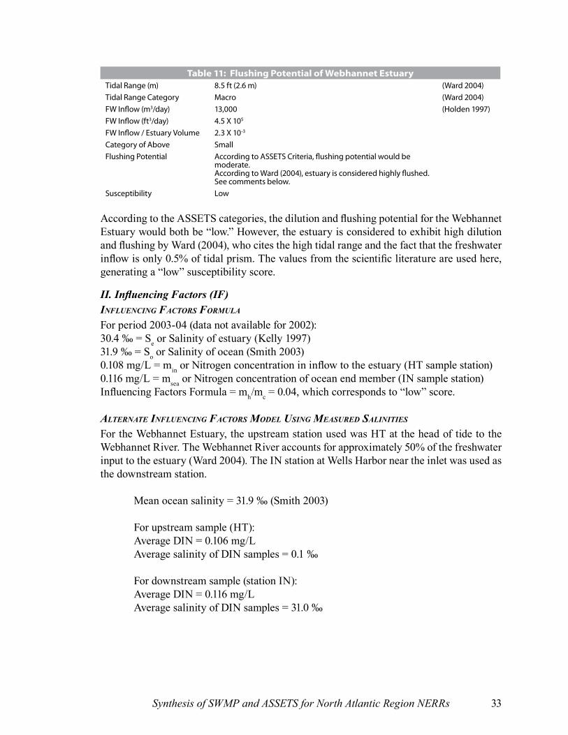
Synthesis of SWMP and ASSETS for North Atlantic Region NERRs 33
Table 11: Flushing Potential of Webhannet EstuaryTidal Range (m) 8.5 ft (2.6 m) (Ward 2004)Tidal Range Category Macro (Ward 2004)FW Inflow (m3/day) 13,000 (Holden 1997)FW Inflow (ft3/day) 4.5 X 10⁵
FW Inflow / Estuary Volume 2.3 X 10⁻³
Category of Above SmallFlushing Potential According to ASSETS Criteria, flushing potential would be
moderate. According to Ward (2004), estuary is considered highly flushed. See comments below.
Susceptibility Low
According to the ASSETS categories, the dilution and flushing potential for the Webhannet Estuary would both be “low.” However, the estuary is considered to exhibit high dilution and flushing by Ward (2004), who cites the high tidal range and the fact that the freshwater inflow is only 0.5% of tidal prism. The values from the scientific literature are used here, generating a “low” susceptibility score.
II. Influencing Factors (IF)inFluencing Factors Formula
For period 2003-04 (data not available for 2002):30.4 ‰ = Se or Salinity of estuary (Kelly 1997)31.9 ‰ = So or Salinity of ocean (Smith 2003)0.108 mg/L = min or Nitrogen concentration in inflow to the estuary (HT sample station)0.116 mg/L = msea or Nitrogen concentration of ocean end member (IN sample station)Influencing Factors Formula = mh/mc = 0.04, which corresponds to “low” score.
alternate inFluencing Factors moDel using measureD salinities
For the Webhannet Estuary, the upstream station used was HT at the head of tide to the Webhannet River. The Webhannet River accounts for approximately 50% of the freshwater input to the estuary (Ward 2004). The IN station at Wells Harbor near the inlet was used as the downstream station.
Mean ocean salinity = 31.9 ‰ (Smith 2003)
For upstream sample (HT):Average DIN = 0.106 mg/LAverage salinity of DIN samples = 0.1 ‰
For downstream sample (station IN):Average DIN = 0.116 mg/LAverage salinity of DIN samples = 31.0 ‰
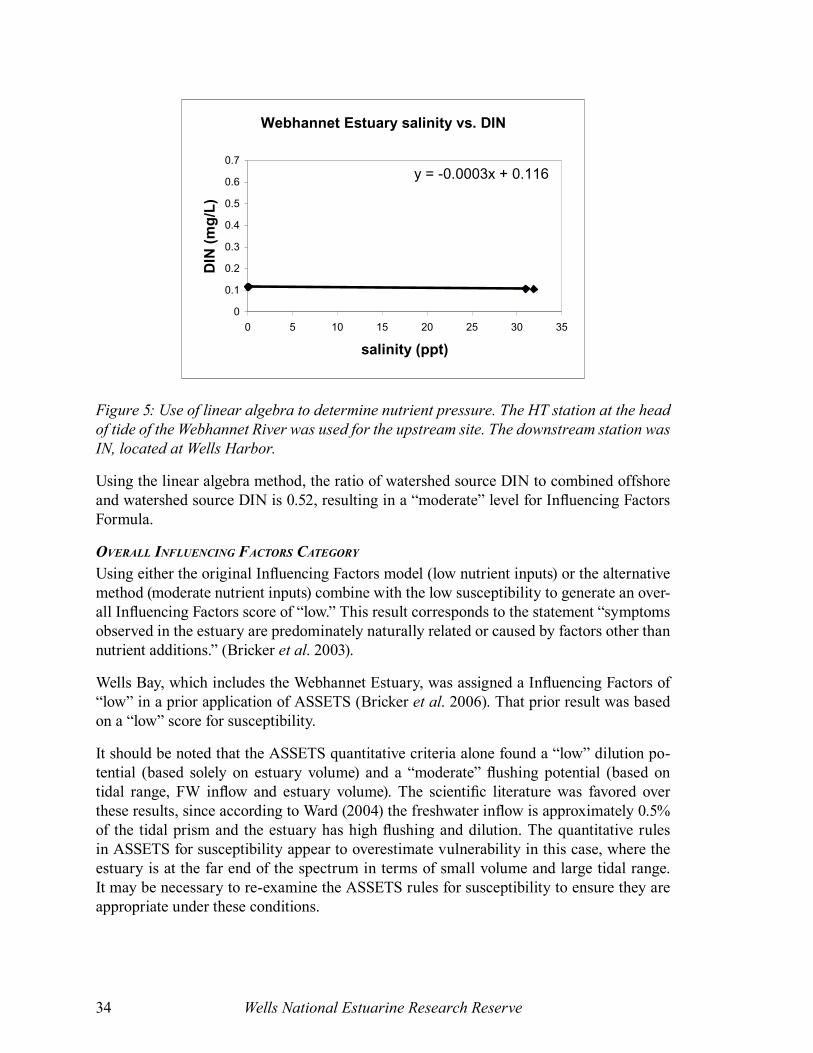
Wells National Estuarine Research Reserve34
Webhannet Estuary salinity vs. DIN
y = -0.0003x + 0.116
0
0.1
0.2
0.3
0.4
0.5
0.6
0.7
0 5 10 15 20 25 30 35
salinity (ppt)
DIN
(mg
/L)
Great Bay salinity vs. DIN
y = -0.0074x + 0.3055
0
0.1
0.2
0.3
0.4
0.5
0.6
0.7
0 5 10 15 20 25 30 35
salinity (ppt)
DIN
(mg
/L)
MBLR Estuary salinity vs. DIN
y = 0.0029x + 0.0954
0
0.1
0.2
0.3
0.4
0.5
0.6
0.7
0 10 20 30 40
salinity (ppt)
DIN
(mg
/L)
Waquoit Bay salinity vs. DIN
y = -0.0117x + 0.3843
0
0.1
0.2
0.3
0.4
0.5
0.6
0.7
0 5 10 15 20 25 30 35
salinity (ppt)D
IN(m
g/L
)
Figure 5: Use of linear algebra to determine nutrient pressure. The HT station at the head of tide of the Webhannet River was used for the upstream site. The downstream station was IN, located at Wells Harbor.
Using the linear algebra method, the ratio of watershed source DIN to combined offshore and watershed source DIN is 0.52, resulting in a “moderate” level for Influencing Factors Formula.
overall inFluencing Factors category
Using either the original Influencing Factors model (low nutrient inputs) or the alternative method (moderate nutrient inputs) combine with the low susceptibility to generate an over-all Influencing Factors score of “low.” This result corresponds to the statement “symptoms observed in the estuary are predominately naturally related or caused by factors other than nutrient additions.” (Bricker et al. 2003).
Wells Bay, which includes the Webhannet Estuary, was assigned a Influencing Factors of “low” in a prior application of ASSETS (Bricker et al. 2006). That prior result was based on a “low” score for susceptibility.
It should be noted that the ASSETS quantitative criteria alone found a “low” dilution po-tential (based solely on estuary volume) and a “moderate” flushing potential (based on tidal range, FW inflow and estuary volume). The scientific literature was favored over these results, since according to Ward (2004) the freshwater inflow is approximately 0.5% of the tidal prism and the estuary has high flushing and dilution. The quantitative rules in ASSETS for susceptibility appear to overestimate vulnerability in this case, where the estuary is at the far end of the spectrum in terms of small volume and large tidal range. It may be necessary to re-examine the ASSETS rules for susceptibility to ensure they are appropriate under these conditions.

Synthesis of SWMP and ASSETS for North Atlantic Region NERRs 35
Overall, the low result for Influencing Factors is consistent with prior studies. Historically, the Webhannet Estuary has not been considered to suffer from high nutrient pressure. A study of estuaries in the Gulf of Maine in 1996 showed the Webhannet’s mean DIN concen-tration of 2.2 µg/L, while the MBLR was about double that at 4.7 µg/L. Both concentrations were noted as very low compared to other estuaries around the nation (Kelly 1997).
III. Overall Eutrophic Condition (OEC)Table 12: Salinity Zones of Webhannet Estuary
Surface Area of Total Estuary (m2) 1,307,318
Salinity Zones Seawater Mixing Freshwater TidalSurface Area (m2) 1,098,211 209,107 0Zone Area / Total Area 0.84 0.16 0
Figure 6: Salinity zones were updated using higher resolution coverage of the estuary and additional data from Wells NERR SWMP and Watershed Evaluation Team.

Wells National Estuarine Research Reserve36
chloroPhyll-a
A prior study by Kelly (1997) found low levels of chlorophyll-a and other nutrients in estu-aries throughout the northern Gulf of Maine, including the Webhannet. High flushing due to large tidal range was cited as protecting these estuaries from eutrophication. However, lower salinities were correlated with higher nutrients and lower dissolved oxygen, suggest-ing that they were not completely immune from land-based influences.
The data used for this study generally confirm this finding. Yearly 90th percentiles of chlo-rophyll-a from the SWMP database indicate medium levels at site HT (head of tide) for two of three years, with all other sites showing low levels. Using medium concentrations at medium spatial distribution and episodic frequency results in low expression value for Chl-a.
Additional data: The WET program data (high school & junior high volunteer data, no formal QA/QC) is currently undergoing data entry for the study period, and data is avail-able only for years 1992-1998. Keeping in mind the limitations of this dataset, it shows a 90th percentile only slightly above 5 µg/L only for the mixing zone, while the seawater zone shows “low” levels. Since these values are not for the study period, they are not included in the ASSETS score here.
macroalgae
Macroalgae has not been formally studied, but personal observations by Dalton and Dionne (personal communication) indicate it was not a problem for biological resources during this time period. Expression value is considered “no problem” for macroalgae, although evidence is limited to informal observations.
DissolveD oxygen
Historically, dissolved oxygen has not been a problem at Wells NERR. Ward’s (1993) measurements from May 1990 to June 1992 showed levels were generally well above any problem threshold, although minimum values occasionally dipped into the biological stress range (<5 mg/L). Only on two days during that period and only at Wells Harbor did DO fall below 3 mg/L, perhaps an early indication of some degree of susceptibility to low DO at that site.
Kelly et al. (1996) conducted a survey of dissolved oxygen in 1995 in the Gulf of Maine from New Hampshire to Canada (but not including the Webhannet Estuary). This study was repeated the following year, covering more estuaries and including the Webhannet, (Kelly 1997). Dissolved oxygen levels in the region were high, only about 1.5% of Maine samples <5.5 mg/L, showing lowest levels in September. Despite generally high levels in both the Webhannet and MBLR estuaries, these estuaries were in the lower range for Maine indicating perhaps slightly higher susceptibility than neighboring estuaries.
Given the high resolution of SWMP data, this report uses monthly 10th percentile for dis-solved oxygen. According to this measure, the mixing zone shows episodic biological stress across the study period. However, in the seawater zone (which is monitored at only one site), hypoxia occurred during one month in 2002, while the second half of 2004 showed
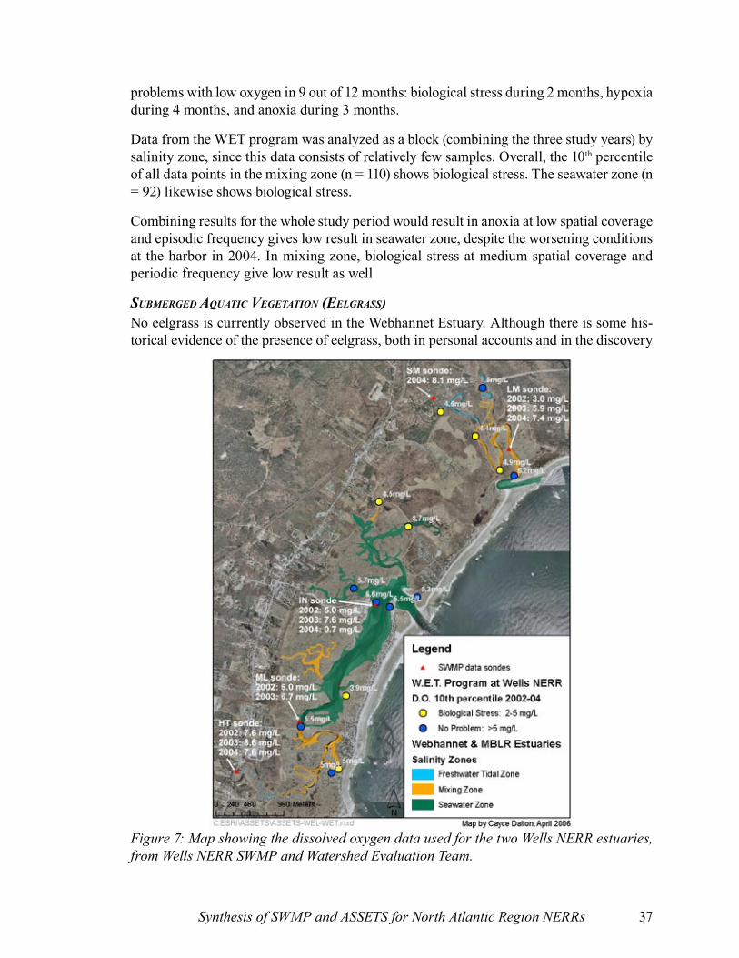
Synthesis of SWMP and ASSETS for North Atlantic Region NERRs 37
problems with low oxygen in 9 out of 12 months: biological stress during 2 months, hypoxia during 4 months, and anoxia during 3 months.
Data from the WET program was analyzed as a block (combining the three study years) by salinity zone, since this data consists of relatively few samples. Overall, the 10th percentile of all data points in the mixing zone (n = 110) shows biological stress. The seawater zone (n = 92) likewise shows biological stress.
Combining results for the whole study period would result in anoxia at low spatial coverage and episodic frequency gives low result in seawater zone, despite the worsening conditions at the harbor in 2004. In mixing zone, biological stress at medium spatial coverage and periodic frequency give low result as well
submergeD aquatic vegetation (eelgrass)No eelgrass is currently observed in the Webhannet Estuary. Although there is some his-torical evidence of the presence of eelgrass, both in personal accounts and in the discovery
Figure 7: Map showing the dissolved oxygen data used for the two Wells NERR estuaries, from Wells NERR SWMP and Watershed Evaluation Team.
Wells National Estuarine Research Reserve38
in 1988 of seed remains in a core sample, none was found in the early 1990’s either (Short et al. 1993). Restoration efforts in 1987 and 1988 resulted in the rapid die-off of transplants, attributed to the exposure due to the high tidal range in the estuary and the dark color of the freshwater inflow which reduced light availability (Short 1993). These factors indicate that at least for the past 15 years there have been no established eelgrass beds at either of the Wells NERR’s estuaries. This symptom is noted as “no change.” Expression of SAV loss is considered “low,” only because no beds are known to exist in the estuary.
hazarDous or nuisance algal blooms (hab)Although paralytic shellfish poison toxin (PSP) has been found in the area (Bean 2004 un-published), the algal blooms which generate it are considered to begin offshore and advect into the estuary. For this reason, the HAB score is considered low.
overall eutroPhic conDition summary
Primary symptoms are “low.”Secondary symptoms are “low.”
Combining primary and secondary symptoms of eutrophication for the entire study period yields a “low” overall eutrophic condition. This score is in spite of repeated periods of anoxia at one sample station in 2004. The ASSETS methodology describes this situation as follows: “level of expression of eutrophic conditions is minimal.” (Bricker et al. 2003).
Despite this assessment, the low oxygen periods in the Webhannet Estuary are a cause for concern and should be investigated further. These conditions persisted throughout the fall into early winter when low oxygen would not be expected. The sample station is surround-ed by docks at the harbor. The timing and location of oxygen depletion might be caused by human activity at the dock, which might have only localized effects (e.g., overboard discharge of solid wastes which settle near the data sonde). Another possible explanation is that shifting sediments have created a depression around the Webhannet Inlet sonde, and this micro-zone is prone to poor mixing dynamics. Given the large tidal range, this would seem unlikely. Nonetheless, the dilution and flushing, according to the ASSETS model, are both less than what was previously thought (compare to ASSETS GOM Pilot Study). A third explanation is that conditions in the deployment tube might be causing readings which do not represent general conditions in the estuary. For example, algae could be growing on the deployment tube, consuming oxygen during certain periods and lowing readings in the immediate vicinity of oxygen probe. Or, somehow water exchange between the inside and outside of the tube could somehow be blocked. Both of these possibilities can be evaluated relatively easily. Further investigation is needed to determine if data from the Webhannet Inlet sonde represent the general conditions in the seawater zone of the estuary.
IV. Future Outlook (FO)The Webhannet Watershed is among the least developed in this study. However, the wa-tershed has shown approximately 50% growth in housing in the past ten years (Wells NERR 2003). Since that time, additional housing construction has been strong in the area. An example of new construction includes a new multifamily unit whose lawn and gravel drainage area reaches into the no-build vegetated buffer zone along Blacksmith Brook in a
Synthesis of SWMP and ASSETS for North Atlantic Region NERRs 39
previously undeveloped area (McBride, pers. comm.). Such an example sets a precedent of builders bringing new sources of nutrients directly to the stream banks, undermining effec-tiveness of legislation designed to protect the estuary from eutrophication. Nutrient inputs from land based sources can be expected to increase significantly, given these trends.
Expected nutrient trends, combined with the high susceptibility result in a “worsen high” score for Future Outlook, which corresponds to the statement “nutrient related symptoms are likely to substantially worsen.” This is what appears to be happening at the Wells Harbor station (IN). The periods of low dissolved oxygen which appeared in the second half of 2004 became more severe and persistent in 2005 and the first half of 2006. It may be that low observed dissolved oxygen at this station is due to highly localized conditions, for example high biological oxygen demand from organic matter deposited near the sonde, in particular if sediments have eroded to form a depression around the deployment tube. On the other hand, if conditions at that sample station prove to be representative of general estuarine conditions, the change toward more severe signs of eutrophication may already be well underway.
V. Overall Classification Grade (ASSETS)Pressure (IF): 5 = LowState (OEC): 5 = LowResponse (FO): 1 = Worsen HighOverall: Good
ReferencesBricker S.D., D. Lipton, A. Mason, M. Dionne, D. Keeley, C. Krahforst, J. Latimer, J. Pennock. 2006. Improving methods and indicators for evaluating coastal water eutrophica-tion: a pilot study in the Gulf of Maine. Report to NOAA-CICEET. 66p.
Holden, William F. 1997. Fresh Water, Suspended Sediment, and Nutrient Influx to the Little River and Webhannet River Estuaries, Wells, Maine. Dissertation, Boston University. 258 p.
Kelly, J.R. and P.S. Libby. 1996. Final Report on Dissolved Oxygen Levels in Select Maine Estuaries and Embayments. Report submitted to Wells NERR and Maine Dept. of Environmental Protection Marine Program. Battelle Ocean Sciences, Duxbury MA. 46p.
Kelly, J.R. 1997. Final Report Dissolved Oxygen in Maine Estuaries and Embayments: 1996 Results and Analyses. Report submitted to Wells NERR and Maine Dept. of Environmental Protection, and Casco Bay Estuary Project. 95 p.
Mariano, C.G. 1989. Wave-current interactions at the Wells inlet and a comparison of hy-draulics and sand circulation with the Little River inlet. Boston University, Boston, MA.
Short, F. T., D. M. Burdick, J. S. Wolf and G. E. Jones. 1993. Eelgrass in Estuarine Research Reserves along the East Coast, USA. Part I: Declines from pollution and disease; Part II: Management of eelgrass meadows. NOAA, Coastal Ocean Program through the Sea Grant College Program, 107 pp.
Wells National Estuarine Research Reserve40
Smith, S.V. 2003. Preliminary NOAA estuarine typology database.
Southern Maine Regional Planning Commission. 2000. Profile of General Demographic Characteristics. Springvale, ME. http://www.smrpc.org/census/censusprofiles/Wells.pdf
Ward LG. 2004. Variations in physical properties and water quality in the Webhannet River estuary (Wells National Estuarine Research Reserve, Maine). Journal of Coastal Research Special Issue 45:39-58.
Wells National Estuarine Research Reserve (WNERR). 2003. Webhannet River
Watershed Conservation Strategy report: summary handout. Maine Department of Environmental Protection.
Wells National Estuarine Research Reserve (WNERR). 2002. Merriland, Branch, and Little River Watershed Shoreland Survey of Non-point Sources. Maine Department of Environmental Protection.
Whiting-Grant, K., C. Dalton, F. Dillon. 2003. Microbial Source Tracking in Two Southern Maine Watersheds: Webhannet River Watershed Report. Maine Sea Grant report no. MSG-TR-03-01.

Synthesis of SWMP and ASSETS for North Atlantic Region NERRs 41
Merriland / Branch / Little River (MBLR) EstuaryThe Merriland / Branch Brook / Little River (MBLR) Estuary is the second of two estuaries located at Wells NERR in Maine. Its watershed is about 80 km2 (Holden 1997), about twice as large as the adjacent Webhannet. Discharge of the Little River also over twice that of Webhannet (see statistics below). The watershed extends about 10 miles inland, narrow-ing sharply as it reaches the coast. Despite the larger watershed area and discharge, the estuary itself is much smaller (1.2% of watershed’s land cover is estuarine marsh) than the Webhannet. The watershed is less developed than the Webhannet, showing about 3% de-veloped land cover compared to the 9% using the same methodology as for the Webhannet (Whiting-Grant 2004). Development has been primarily been single house lots or small developments, although a large golf course and residential complex has been recently pro-posed (WNERR 2004), and a condominium village is now under construction adjacent to the Merriland River in close proximity to the Little River Estuary, and other similar devel-opments are now in the planning stages. No population figures are available specifically for the watershed, although 1281 developed land parcels were recently counted (WNERR 2004). An estimate of two residents per developed parcel would suggest a population be-tween 2000 and 3000. The estuary system itself is the only undeveloped barrier beach and salt marsh in Maine with a tidal inlet (WNERR 2003). The MBLR has not been evaluated separately under any previous NEEA or ASSETS application, since it is a component of Wells Bay.
Data SourcesAlthough currently there are two SWMP sondes in the MBLR Estuary, in 2002-2003 there was only one. In 2002, that sonde was deployed for only three months in the spring due to difficulties with site stability, although nutrient samples were collected from April through December. By contrast, the WET Program has sampled continuously from the early 1990’s to the present. WET data is collected by high school and junior high students and has not undergone full QA/QC, nonetheless it provides some level of information in areas which are not otherwise sampled.
The SWMP program has one sample station in the mixing zone (LM) and one in the freshwater tidal zone (SM). The upstream sample station was inadvertently established just upstream of the head of tide, however it is considered in an estuarine zone for this study. The sonde has since been moved to within the mixing zone. The WET program has 5 sample stations in the estuary, plus one at the initial logger stations just upstream of the head of tide.
I. SusceptibilityTable 13: Dilution Potential of MBLR Estuary
Vertical Stratification Minor (Dionne, pers. comm. 2006) Volume of Estuary (m3) 495,000 (Holden 1997)Volume of Estuary (ft3) 17,400,000Volume of FW Fraction Not neededDilution Value (1/volume ft3) 5.72 x 10⁻⁸ ~ 10-7 on log scaleDilution Potential Low

Wells National Estuarine Research Reserve42
Table 14: Flushing Potential of MBLR EstuaryTidal Range (m) 8.6 ft (2.6 m) (Ward 2004)Tidal Range Category MacroFW Inflow (m3/day) 31000 (Holden 1997)FW Inflow (ft3/day) 1.1 x 10⁶
FW Inflow / Estuary Volume 6.3 x 10⁻² ~ 10-1 given log scaleCategory of Above LargeFlushing Potential HighSusceptibility Moderate
II. Influencing Factors (IF)inFluencing Factors Formula
For period 2003-04 (data not available for 2002):18.1 ‰ = So or Salinity of estuary (Kelly 1997)31.9 ‰ = So or Salinity of ocean (Smith 2003)0.096 mg/L = min or Nitrogen concentration in inflow to the estuary (SM sample station)0.130 mg/L = msea or Nitrogen concentration of ocean end member (LM sample station)Influencing Factors Formula = mh/mc = 0.36, which corresponds to “moderate” score.
alternate inFluencing Factors moDel using measureD salinities
The intersection of the lines from two stations (furthest upstream and furthest downstream) are used to determine the ratio of sources for the estuary. For the MBLR Estuary, the SM site located just above the head of tide in the Merriland River was used as the up-stream station. This choice was dictated by the location of the SWMP site locations. The other major tributary to the estuary, Branch Brook, was considered the primary source of
Figure 8: Use of linear algebra to determine nutrient pressure. The Skinner Mill station was used for the upstream site, although this accounts only for the Merriland River fresh-water input, excluding the Branch Brook. The downstream station was the Little River mouth station.
Webhannet Estuary salinity vs. DIN
y = -0.0003x + 0.116
0
0.1
0.2
0.3
0.4
0.5
0.6
0.7
0 5 10 15 20 25 30 35
salinity (ppt)
DIN
(mg
/L)
Great Bay salinity vs. DIN
y = -0.0074x + 0.3055
0
0.1
0.2
0.3
0.4
0.5
0.6
0.7
0 5 10 15 20 25 30 35
salinity (ppt)
DIN
(mg
/L)
MBLR Estuary salinity vs. DIN
y = 0.0029x + 0.0954
0
0.1
0.2
0.3
0.4
0.5
0.6
0.7
0 10 20 30 40
salinity (ppt)
DIN
(mg
/L)
Waquoit Bay salinity vs. DIN
y = -0.0117x + 0.3843
0
0.1
0.2
0.3
0.4
0.5
0.6
0.7
0 5 10 15 20 25 30 35
salinity (ppt)
DIN
(mg
/L)

Synthesis of SWMP and ASSETS for North Atlantic Region NERRs 43
nitrates+nitrites by Holden 1997. The downstream site was the LM station located near the mouth of the estuary.
Mean ocean salinity = 31.9 ‰ (Smith 2003)
For upstream sample (WEL SM):Average DIN = 0.096 mg/LAverage salinity of DIN samples = 0.1 ‰
For downstream sample (WEL LM):Average DIN = 0.125 mg/LAverage salinity of DIN samples = 10.3 ‰
Using the linear algebra approach, the ratio of watershed-based DIN to total DIN is 0.39. This alternative method indicates a very similar Influencing Factors score as the above method in the “moderate” range.
overall inFluencing Factors category
The “moderate” nutrient loading score combined with the “moderate” susceptibility result in an overall Influencing Factors score of “moderate,” which corresponds to the descrip-tion, “symptoms observed in the estuary are moderately related to nutrient inputs” (Bricker et al. 2003).
III. Overall Eutrophic Condition (OEC)Table 15: Salinity Zones of MBLR Estuary
Surface Area of Total Estuary (m2) 203,023
Salinity Zones Seawater Mixing Freshwater TidalSurface Area (m2) 57,353 145,670 0Zone Area / Total Area 0.28 0.72 0
chloroPhyll-a
Yearly 90th percentiles of chlorophyll-a from the SWMP database show that in 2002 and 2004 levels were low. In 2003, levels were slightly above the “medium” threshold.
Additional data is available from the WET program. These data are currently undergoing data entry for the study period, and data is available only for years 1992-1998. Keeping in mind the limitations of this dataset, it shows a 90th percentile only slightly above 5 µg/L only for the mixing zone, while the seawater zone shows “low” levels. The overall expres-sion value is low for Chl-a.
macroalgae
Macroalgae has not been formally studied, but personal observations by Dalton and Dionne indicate it was not a problem for biological resources during this time period. Expression value is considered “no problem” for macroalgae, although evidence is limited to informal observations.
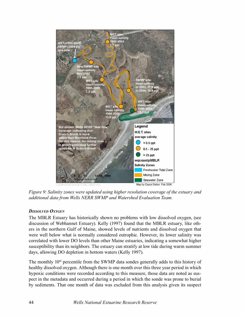
Wells National Estuarine Research Reserve44
DissolveD oxygen
The MBLR Estuary has historically shown no problems with low dissolved oxygen, (see discussion of Webhannet Estuary). Kelly (1997) found that the MBLR estuary, like oth-ers in the northern Gulf of Maine, showed levels of nutrients and dissolved oxygen that were well below what is normally considered eutrophic. However, its lower salinity was correlated with lower DO levels than other Maine estuaries, indicating a somewhat higher susceptibility than its neighbors. The estuary can stratify at low tide during warm summer days, allowing DO depletion in bottom waters (Kelly 1997).
The monthly 10th percentile from the SWMP data sondes generally adds to this history of healthy dissolved oxygen. Although there is one month over this three year period in which hypoxic conditions were recorded according to this measure, those data are noted as sus-pect in the metadata and occurred during a period in which the sonde was prone to burial by sediments. That one month of data was excluded from this analysis given its suspect
Figure 9: Salinity zones were updated using higher resolution coverage of the estuary and additional data from Wells NERR SWMP and Watershed Evaluation Team.

Synthesis of SWMP and ASSETS for North Atlantic Region NERRs 45
nature. Only in one other month (site LM, October 2003) did DO dip into the biological stress level at 4 mg/L.
This study used the 10th percentile of all WET data from each site over the study period, given the relatively few water samples, and the increased possibility of outliers due to student error. Using this metric, the WET data indicates biological stress in some areas of mixing zone and seawater zone. (See Webhannet section for DO map.)
Taken together, the data indicate episodic conditions of biological stress, which at any level of spatial frequency, indicate a “low” score for dissolved oxygen. Overall, dissolved oxygen symptom is considered low for all three years.
submergeD aquatic vegetation (eelgrass)There have been no established eelgrass beds in the MBLR estuary for at least the past 15 years. See SAV under the Webhannet Estuary above. Expression of SAV loss is considered “low,” only because no beds are known to exist in the estuary.
hazarDous or nuisance algal blooms (hab)The HAB score is considered low, due to the fact that in Wells Bay (which includes the MBLR Estuary), blooms are considered to occur offshore and advect into the estuaries (Bean 2004 unpublished).
overall eutroPhic conDition summary
Primary symptoms are “low.”Secondary symptoms are “low.”
Combining primary and secondary symptoms of eutrophication yields an overall “low” eu-trophic condition for the study period. The ASSETS methodology describes this situation as follows: “level of expression of eutrophic conditions is minimal” (Bricker et al. 2003).
IV. Future Outlook (FO)The MBLR Watershed is the most rural in this study. Significant tracts of land are owned by the Kennebunk Kennebunkport Wells Water District since drinking water is drawn from Branch Brook. These tracts are currently managed for conservation, although the water district owns them outright and may sell them in the future to fund additional or alternative water infrastructure. There are developments that have the potential to make a strong impact on the watershed, including the large, dense campground located where US Route 1 intersects the Merriland River, and the possibility that farms and fields along much of the rivers will soon become more densely developed. For example, a new golf course and condominium development has been constructed along the banks of the Merriland within several kilometers of its confluence with the Little River estuary. A third cause for concern is bottled water plant along the Merriland River which could significantly reduce ground-water flow to the estuary, which could result in higher proportions of surface runoff, with a consequent increase in nutrient concentrations. Given these factors, nutrient pressures can be expected to increase somewhat over the coming years, although probably less so than

Wells National Estuarine Research Reserve46
in the Webhannet, which has a much higher proportion of its watershed closer to the coast, where development is particularly aggressive.
Expected increase in nutrients, combined with the moderate susceptibility combine to indi-cate a “worsen high” score for Future Outlook, which corresponds to the statement “nutri-ent related symptoms are likely to substantially worsen” (Bricker et al. 2003).
V. Overall Classification Grade (ASSETS)Pressure (IF): 3 = ModerateState (OEC): 5 = LowResponse (FO): 1 = Worsen HighOverall: Moderate
ReferencesBricker S.D., D. Lipton, A. Mason, M. Dionne, D. Keeley, C. Krahforst, J. Latimer, J. Pennock. 2006. Improving methods and indicators for evaluating coastal water eutrophica-tion: a pilot study in the Gulf of Maine. Report to NOAA-CICEET. 66 p.
Holden, William F. 1997. Fresh Water, Suspended Sediment, and Nutrient Influx to the Little River and Webhannet River Estuaries, Wells, Maine. Dissertation, Boston University. 258 p.
Kelly, J.R. and P.S. Libby. 1996. Final Report on Dissolved Oxygen Levels in Select Maine Estuaries and Embayments. Report submitted to Wells NERR and Maine Dept. of Environmental Protection Marine Program. Battelle Ocean Sciences, Duxbury MA. 46p.
Kelly, J.R. 1997. Final Report Dissolved Oxygen in Maine Estuaries and Embayments: 1996 Results and Anayses. Report submitted to Wells NERR and Maine Dept. of Environmental Protection, and Casco Bay Estuary Project. 95 p.
Smith, S.V. 2003. Preliminary NOAA estuarine typology database.
Ward LG. 2004. Variations in physical properties and water quality in the Webhannet River estuary (Wells National Estuarine Research Reserve, Maine). Journal of Coastal Research Special Issue 45:39-58.
Wells National Estuarine Research Reserve (WNERR). 2003. MBLR Watershed Conservation Strategy report: summary handout. Maine Department of Environmental Protection.
Wells National Estuarine Research Reserve (WNERR). 2004. Merriland River, Branch Brook, and Little River Watershed Nonpoint Source Pollution Management Plan. Maine Department of Environmental Protection.
Whiting-Grant, K., C. Dalton, F. Dillon. 2004. Microbial Source Tracking in Two Southern Maine Watersheds: Merriland River, Branch Brook and Little River (MBLR) Watershed Report. Maine Sea Grant report no. MSG-TR-04-01.

Synthesis of SWMP and ASSETS for North Atlantic Region NERRs 47
Great Bay EstuaryGreat Bay Estuary, located at the border between New Hampshire and Maine, is a tide dominated system fed by seven major rivers, and includes Great Bay, Little Bay and the Piscataqua River. The Bay itself extends 25 km inland, with a watershed of 2,409 km2, the largest in this study. The elongated shape of the estuary creates a significant time lag between tides at the mouth and in the bay, up to 2.5 hours, and the flushing time has been estimated at 36 tidal cycle, or 18 days (Short 1992). Development and population are densely concentrated in the coastal region, such as Portsmouth. Population has increased steadily in recent years, and land use has tended to reflect this growth in impervious sur-face (Trowbridge 2006c). Nonetheless, there are still significant tracts of unfragmented lands to the west of Great Bay suggesting the development pressure on a whole across the watershed is moderate, although rates of change have not yet been determined for this indicator (Trowbridge 2006c).
Data SourcesGreat Bay Estuary is the focus of several monitoring programs. There are four SWMP sondes recording dissolved oxygen and salinity (among other parameters) at 30 minute intervals. The SWMP program also generates chlorophyll-a and nitrogen species data from grab samples at these four stations on a monthly basis, excluding ice-season. New Hampshire Estuary Project (NHEP) and University of New Hampshire (UNH) maintain two additional sondes, following nearly identical protocol as SWMP. In addition, the NH Department of Environmental Services (NHDES) collects grab samples from 10 stations throughout the estuary, which are analyzed for dissolved oxygen, chlorophyll-a and various nitrogen components.
Great Bay Coast Watch is a volunteer monitoring program with an EPA approved Quality Assurance Project Plan (QAPP) and more than 10 years of experience. It collects monthly grab samples from 22 sites throughout the estuary at high and low tide which it analyzes for dissolved oxygen, salinity and other parameters.
I. SusceptibilityTable 16: Dilution Potential of Great Bay Estuary
Vertical Stratification HomogeneousVolume of Estuary (m3) 2.3 X 10⁸ (Short 1992)Volume of Estuary (ft3) 8.1 X 10⁹ Vol of FW Fraction Not NeededDilution Value (1/volume ft3) 1.23 X 10⁻¹⁰
Dilution Potential Low
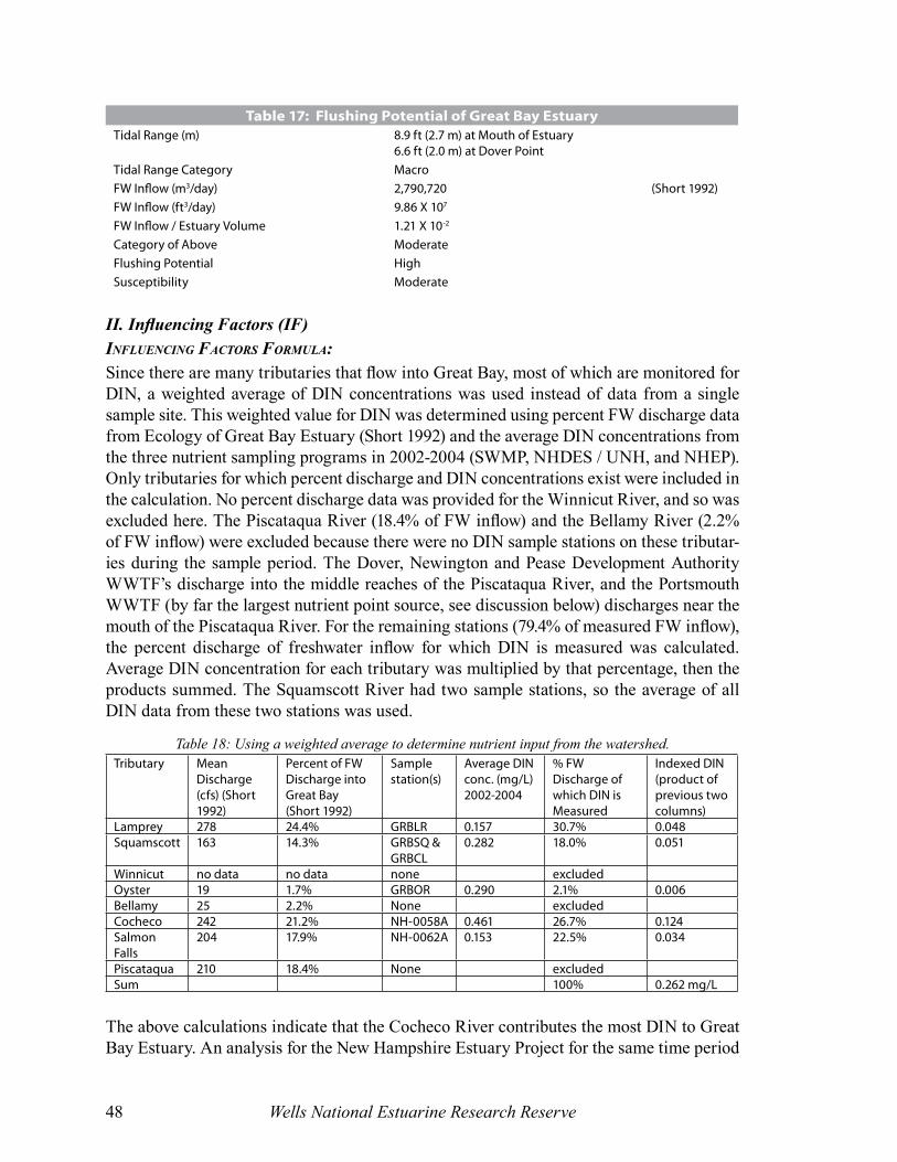
Wells National Estuarine Research Reserve48
Table 17: Flushing Potential of Great Bay EstuaryTidal Range (m) 8.9 ft (2.7 m) at Mouth of Estuary
6.6 ft (2.0 m) at Dover PointTidal Range Category MacroFW Inflow (m3/day) 2,790,720 (Short 1992)FW Inflow (ft3/day) 9.86 X 10⁷
FW Inflow / Estuary Volume 1.21 X 10⁻²
Category of Above ModerateFlushing Potential HighSusceptibility Moderate
II. Influencing Factors (IF)inFluencing Factors Formula:Since there are many tributaries that flow into Great Bay, most of which are monitored for DIN, a weighted average of DIN concentrations was used instead of data from a single sample site. This weighted value for DIN was determined using percent FW discharge data from Ecology of Great Bay Estuary (Short 1992) and the average DIN concentrations from the three nutrient sampling programs in 2002-2004 (SWMP, NHDES / UNH, and NHEP). Only tributaries for which percent discharge and DIN concentrations exist were included in the calculation. No percent discharge data was provided for the Winnicut River, and so was excluded here. The Piscataqua River (18.4% of FW inflow) and the Bellamy River (2.2% of FW inflow) were excluded because there were no DIN sample stations on these tributar-ies during the sample period. The Dover, Newington and Pease Development Authority WWTF’s discharge into the middle reaches of the Piscataqua River, and the Portsmouth WWTF (by far the largest nutrient point source, see discussion below) discharges near the mouth of the Piscataqua River. For the remaining stations (79.4% of measured FW inflow), the percent discharge of freshwater inflow for which DIN is measured was calculated. Average DIN concentration for each tributary was multiplied by that percentage, then the products summed. The Squamscott River had two sample stations, so the average of all DIN data from these two stations was used.
Table 18: Using a weighted average to determine nutrient input from the watershed.Tributary Mean
Discharge (cfs) (Short 1992)
Percent of FWDischarge into Great Bay(Short 1992)
Sample station(s)
Average DIN conc. (mg/L) 2002-2004
% FW Discharge of which DIN is Measured
Indexed DIN (product of previous two columns)
Lamprey 278 24.4% GRBLR 0.157 30.7% 0.048Squamscott 163 14.3% GRBSQ &
GRBCL0.282 18.0% 0.051
Winnicut no data no data none excludedOyster 19 1.7% GRBOR 0.290 2.1% 0.006Bellamy 25 2.2% None excludedCocheco 242 21.2% NH-0058A 0.461 26.7% 0.124Salmon Falls
204 17.9% NH-0062A 0.153 22.5% 0.034
Piscataqua 210 18.4% None excludedSum 100% 0.262 mg/L
The above calculations indicate that the Cocheco River contributes the most DIN to Great Bay Estuary. An analysis for the New Hampshire Estuary Project for the same time period
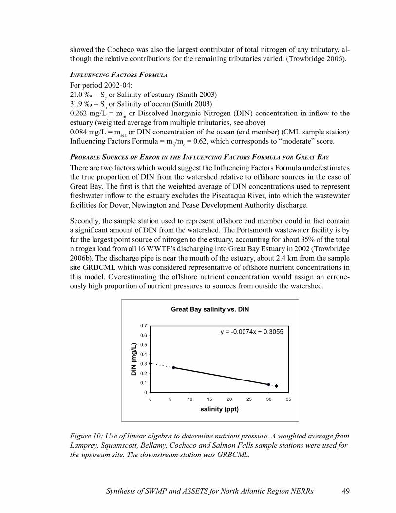
Synthesis of SWMP and ASSETS for North Atlantic Region NERRs 49
showed the Cocheco was also the largest contributor of total nitrogen of any tributary, al-though the relative contributions for the remaining tributaries varied. (Trowbridge 2006).
inFluencing Factors Formula
For period 2002-04:21.0 ‰ = Se or Salinity of estuary (Smith 2003)31.9 ‰ = So or Salinity of ocean (Smith 2003)0.262 mg/L = min or Dissolved Inorganic Nitrogen (DIN) concentration in inflow to the estuary (weighted average from multiple tributaries, see above) 0.084 mg/L = msea or DIN concentration of the ocean (end member) (CML sample station)Influencing Factors Formula = mh/mc = 0.62, which corresponds to “moderate” score.
Probable sources oF error in the inFluencing Factors Formula For great bay
There are two factors which would suggest the Influencing Factors Formula underestimates the true proportion of DIN from the watershed relative to offshore sources in the case of Great Bay. The first is that the weighted average of DIN concentrations used to represent freshwater inflow to the estuary excludes the Piscataqua River, into which the wastewater facilities for Dover, Newington and Pease Development Authority discharge.
Secondly, the sample station used to represent offshore end member could in fact contain a significant amount of DIN from the watershed. The Portsmouth wastewater facility is by far the largest point source of nitrogen to the estuary, accounting for about 35% of the total nitrogen load from all 16 WWTF’s discharging into Great Bay Estuary in 2002 (Trowbridge 2006b). The discharge pipe is near the mouth of the estuary, about 2.4 km from the sample site GRBCML which was considered representative of offshore nutrient concentrations in this model. Overestimating the offshore nutrient concentration would assign an errone-ously high proportion of nutrient pressures to sources from outside the watershed.
Webhannet Estuary salinity vs. DIN
y = -0.0003x + 0.116
0
0.1
0.2
0.3
0.4
0.5
0.6
0.7
0 5 10 15 20 25 30 35
salinity (ppt)
DIN
(mg
/L)
Great Bay salinity vs. DIN
y = -0.0074x + 0.3055
0
0.1
0.2
0.3
0.4
0.5
0.6
0.7
0 5 10 15 20 25 30 35
salinity (ppt)
DIN
(mg
/L)
MBLR Estuary salinity vs. DIN
y = 0.0029x + 0.0954
0
0.1
0.2
0.3
0.4
0.5
0.6
0.7
0 10 20 30 40
salinity (ppt)
DIN
(mg
/L)
Waquoit Bay salinity vs. DIN
y = -0.0117x + 0.3843
0
0.1
0.2
0.3
0.4
0.5
0.6
0.7
0 5 10 15 20 25 30 35
salinity (ppt)
DIN
(mg
/L)
Figure 10: Use of linear algebra to determine nutrient pressure. A weighted average from Lamprey, Squamscott, Bellamy, Cocheco and Salmon Falls sample stations were used for the upstream site. The downstream station was GRBCML.
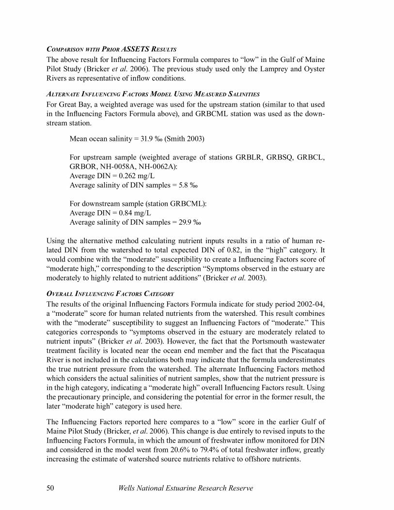
Wells National Estuarine Research Reserve50
comParison With Prior assets results
The above result for Influencing Factors Formula compares to “low” in the Gulf of Maine Pilot Study (Bricker et al. 2006). The previous study used only the Lamprey and Oyster Rivers as representative of inflow conditions.
alternate inFluencing Factors moDel using measureD salinities
For Great Bay, a weighted average was used for the upstream station (similar to that used in the Influencing Factors Formula above), and GRBCML station was used as the down-stream station.
Mean ocean salinity = 31.9 ‰ (Smith 2003)
For upstream sample (weighted average of stations GRBLR, GRBSQ, GRBCL, GRBOR, NH-0058A, NH-0062A):Average DIN = 0.262 mg/LAverage salinity of DIN samples = 5.8 ‰
For downstream sample (station GRBCML):Average DIN = 0.84 mg/LAverage salinity of DIN samples = 29.9 ‰
Using the alternative method calculating nutrient inputs results in a ratio of human re-lated DIN from the watershed to total expected DIN of 0.82, in the “high” category. It would combine with the “moderate” susceptibility to create a Influencing Factors score of “moderate high,” corresponding to the description “Symptoms observed in the estuary are moderately to highly related to nutrient additions” (Bricker et al. 2003).
overall inFluencing Factors category
The results of the original Influencing Factors Formula indicate for study period 2002-04, a “moderate” score for human related nutrients from the watershed. This result combines with the “moderate” susceptibility to suggest an Influencing Factors of “moderate.” This categories corresponds to “symptoms observed in the estuary are moderately related to nutrient inputs” (Bricker et al. 2003). However, the fact that the Portsmouth wastewater treatment facility is located near the ocean end member and the fact that the Piscataqua River is not included in the calculations both may indicate that the formula underestimates the true nutrient pressure from the watershed. The alternate Influencing Factors method which considers the actual salinities of nutrient samples, show that the nutrient pressure is in the high category, indicating a “moderate high” overall Influencing Factors result. Using the precautionary principle, and considering the potential for error in the former result, the later “moderate high” category is used here.
The Influencing Factors reported here compares to a “low” score in the earlier Gulf of Maine Pilot Study (Bricker, et al. 2006). This change is due entirely to revised inputs to the Influencing Factors Formula, in which the amount of freshwater inflow monitored for DIN and considered in the model went from 20.6% to 79.4% of total freshwater inflow, greatly increasing the estimate of watershed source nutrients relative to offshore nutrients.
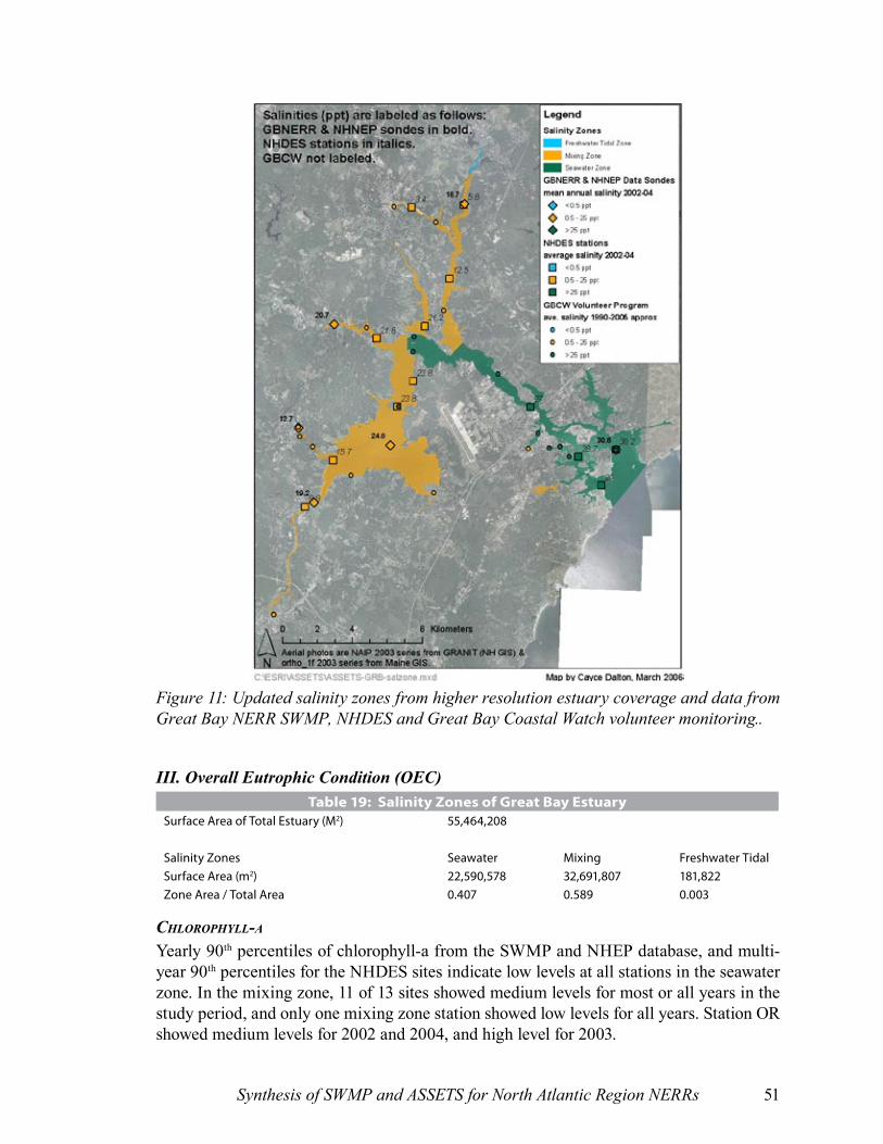
Synthesis of SWMP and ASSETS for North Atlantic Region NERRs 51
Figure 11: Updated salinity zones from higher resolution estuary coverage and data from Great Bay NERR SWMP, NHDES and Great Bay Coastal Watch volunteer monitoring..
III. Overall Eutrophic Condition (OEC)Table 19: Salinity Zones of Great Bay Estuary
Surface Area of Total Estuary (M2) 55,464,208
Salinity Zones Seawater Mixing Freshwater TidalSurface Area (m2) 22,590,578 32,691,807 181,822Zone Area / Total Area 0.407 0.589 0.003
chloroPhyll-a
Yearly 90th percentiles of chlorophyll-a from the SWMP and NHEP database, and multi-year 90th percentiles for the NHDES sites indicate low levels at all stations in the seawater zone. In the mixing zone, 11 of 13 sites showed medium levels for most or all years in the study period, and only one mixing zone station showed low levels for all years. Station OR showed medium levels for 2002 and 2004, and high level for 2003.

Wells National Estuarine Research Reserve52
Expression value for Chl-a is low for seawater zone. Expression value is high for mixing zone, based on medium concentration, periodic frequency and high spatial coverage. The overall expression value for chlorophyll-a for Great Bay is high.
Great Bay is not normally thought of as suffering from high chl-a. Trowbridge (2006b) found that the estuary is meeting the NHEP goal, which is to have no areas in the estuary which exceed the state’s swimming standards of 20 µg/L. In fact, the data used for this study, except for one year at site OR, show that the 90th percentile chlorophyll-a did not exceed this level, and the classification of “high” here is due to samples in the 5-20 µg/L range occurring frequently and over a large area.
macroalgae
Art Mathieson (pers. comm. 2005) stated that problems with macroalgae occur on an an-nual basis in the spring and summer in the Great Bay Estuary, likely due to nutrients released from wastewater treatment facilities. In addition, macroalgae as a symptom of eutrophication were cited by Brian Smith of Great Bay NERR in the mixing zone.
Fred Short (personal comm., 2005) specified that macroalgae is a problem for eelgrass in the central part of the bay, and in the Oyster, Bellamy and Piscataqua rivers. He estimated a 50% increase in recent years, noting that quantification is difficult since algal mats are not attached and move in response to currents and wind. Given the periodic frequency of macroalgae blooms, this symptom is scored as “high.”
DissolveD oxygen
Given the high resolution of SWMP sonde data (30 minute sample interval), monthly 10th percentiles were examined for dissolved oxygen. Additional data comes from NHEP, NHDES, UNH and GBCW grab samples. Given the low number of samples at these sourc-es, this study looked at their 10th percentile for the entire study period (n~30 for NHEP and NHDES, n~45 for GBCW). According to these two measures, only three sites (CL, LR, OR) showed DO values in the biological stress range, and all other sites showed no problem (>5 mg/L). These three sites all occur in the mixing zone, all considerably upstream in tidal river channels. For this reason, the spatial coverage of biological stress was considered very low (>0 and ≤10% of the mixing zone). As a result, dissolved oxygen appears to be a very minor problem for the estuary as a whole, and it’s score falls in the “low” range.
submergeD aquatic vegetation (sav or eelgrass)Generally, the coverage of eelgrass in Great Bay is extensive, thanks in large part to favor-able conditions in the 1980’s that limited the disease which attacks the plant. Fred Short, who has studied eelgrass in Great Bay and the northeast region, states (pers. comm.) that eelgrass coverage in the mixing zone in 2002-03 did not increase, although its biomass did increase. In 2003-04, there was an 18% decline. In the seawater zone, there was no decrease due to eutrophication in eelgrass, although Canada Geese grazing caused a loss near the mouth of the bay. Likewise, Trowbridge (in press) cites that 2004 eelgrass coverage is similar to that observed throughout the 1990’s at about 2000 acres, or about 17% less than the peak in 1996.
Synthesis of SWMP and ASSETS for North Atlantic Region NERRs 53
NHEP looked at long term eelgrass trends, including coverage, density and temporal fre-quency. Biomass in 2004 is 41% less than in 1996, indicating that coverage alone may not be adequate to assess the health of eelgrass in Great Bay. The gradual nature of the decline seems inconsistent with a wasting disease (slime mold, Labryrinthula zosterae) hypothesis. Increasing macroalgal presence appears to be a more plausible explanation and is consistent with anecdotal reports (Trowbridge, in press).
Given the relatively small loss of eelgrass during the study period, the SAV symptom falls in the “low” category. However, this decline is part of a gradual decline on a decadal scale, particularly noticeable in terms of biomass, which is not assessed by ASSETS.
hazarDous or nuisance algal blooms (hab)Both Fred Short and Brian Smith commented that HAB’s have not been seen as a signifi-cant problem in Great Bay Estuary, and is scored as “no problem.”
overall eutroPhic conDition summary
Primary symptoms are “high.”Secondary symptoms are “low”.
Combining primary and secondary symptoms of eutrophication yields an overall “moder-ate” eutrophic condition for the study period, corresponding to the statement, “primary symptoms high but secondary symptoms still not being expressed” (Bricker et al. 2003)
IV. Future Outlook (FO)Population trends indicate a 5-10% increase in population from 2003-2008 in coastal New Hampshire, although upper portions of the watershed will undergo less of a change (Crossett et al. 2004). Impervious surfaces have also increased grown in coastal New Hampshire over the past 15 years, and the rate of increase has increased slightly in the past 5 years. New Hampshire Estuary Project’s goal of limiting impervious surface to no more than 10% of land cover has already been exceeded in 10 of the 37 coastal watersheds and 13 of the 42 coastal municipalities across the state, many in the Great Bay watershed (Trowbridge 2006c). Given these trends and the moderate susceptibility, the FO for Great Bay is as-signed a “worsen high” score.
V. Overall Classification Grade (ASSETS)Pressure (IF): 3 = ModerateState (OEC): 3 = ModerateResponse (FO): 1 = Worsen HighOverall: Poor
ReferencesBricker SD, Lipton D, Mason A, Dionne M, Keeley D, Krahforst C, Latimer J, Pennock J. 2006. Improving methods and indicators for evaluating coastal water eutrophication: a pilot study in the Gulf of Maine. Report to NOAA-CICEET. 66p.
Wells National Estuarine Research Reserve54
Crossett, K. M., T. J. Culliton, P.C. Wiley, T. R. Goodspeed. 2004. Population Trends Along the Coastal United States: 1980-2008. National Oceanic and Atmospheric Administration, National Ocean Service, Management and Budget Office, Special Projects. Coastal Trends Report Series.
Trowbridge, P. March 2006a. Environmental Indicator Report: Critical Habitats and Species. New Hampshire Estuaries Project, University of New Hampshire, Durham, NH.
Trowbridge, P. March 2006b. Environmental Indicator Report: Water Quality. New Hampshire Estuaries Project, University of New Hampshire, Durham, NH.
Trowbridge, P. May 2006c. Environmental Indicator Report: Land Use and Development. New Hampshire Estuaries Project, University of New Hampshire, Durham, NH.
Trowbridge, P. 2006d. State of the Estuaries Report. New Hampshire Estuaries Project, University of New Hampshire, Durham, NH. In press.
Short, FT. 1992. (ed.) The Ecology of the Great Bay Estuary, New Hampshire and Maine: An Estuarine Profile and Bibliography. NOAA-Coastal Ocean Program Publ. 222 pp.
Smith, SV. 2003. Preliminary NOAA estuarine typology database.

Synthesis of SWMP and ASSETS for North Atlantic Region NERRs 55
Waquoit Bay EstuaryWaquoit Bay Estuary is a coastal lagoon system with a large circular basin fed by six diverse sub-embayments (Brawley 2002). Waquoit Bay’s watershed is located on the south-ern side of Cape Cod in the towns of Falmouth, Mashpee, and Sandwich, Massachusetts. This small watershed (65 km2) extends roughly 10 km inland (Cambareri et al. 1998) and consists of dense residential development adjacent to the estuary, with the overwhelming majority of waste treatment through septic systems located in sandy, permeable soils. As a result, the vast majority of nitrogen influx to the estuary occurs via groundwater seepage (Brawley 2002). The bay itself was once a highly productive shellfish area, although eutro-phication has led to declines in this resource. Nonetheless, the bay was one of the only areas in Falmouth re-opened to shellfishing in 2000 due to contamination in adjacent shellfishing waters (MA EOEA 2003).
Data SourcesThere are four SWMP sondes in Waquoit Bay Estuary recording DO, salinity and other parameters at 30 minute intervals. Three sondes are in the seawater zone (over 25 ppt), and one (CR) is in the mixing zone. The SWMP sonde at MH is deployed year round. At other sites, sondes are deployed during the ice-free season, missing only winter and early spring.
In addition, since 1993 there has been a volunteer monitoring program called Baywatchers, which does not undergo the thorough QA/QC of SWMP but greatly increases the spatial coverage of data in the bay. Six of eight Baywatcher sites are in the seawater zone, with two in the mixing zone, including site 7 at the same location as sonde CR. Baywatchers collects samples 16 times per year (once per month, and twice in June, July, August and September) for dissolved oxygen (surface, bottom and sometimes middle), salinity, chlorophyll-a and nutrients.
I. SusceptibilityTable 20: Dilution Potential of Waquoit Bay Estuary
Vertical Stratification Minor (WQB Metadata 2004)Volume of Estuary (m3) 10,770,000 (Howes, et al. 2005)Volume of Estuary (ft3) 3.8 X 10⁸
Vol of FW Fraction Not NeededDilution Value (1/volume ft3) 2.63 X 10⁻⁹
Dilution Potential Low Table 21: Flushing Potential of Waquoit Bay Estuary
Tidal Range 1.5 ft (0.46 m) (Howes, et al. 2005)Tidal Range Category MicroFW Inflow (m3/day) 2.49 X 10⁷, Incl. Groundwater (Cambereri et al. 1998)FW Inflow (ft3/day) 2.41 X 10⁶
FW Inflow / Estuary Volume 6.3 X 10⁻³ ~ 10-2 Given Log ScaleCategory of Above LargeFlushing Potential HighSusceptibility Moderate
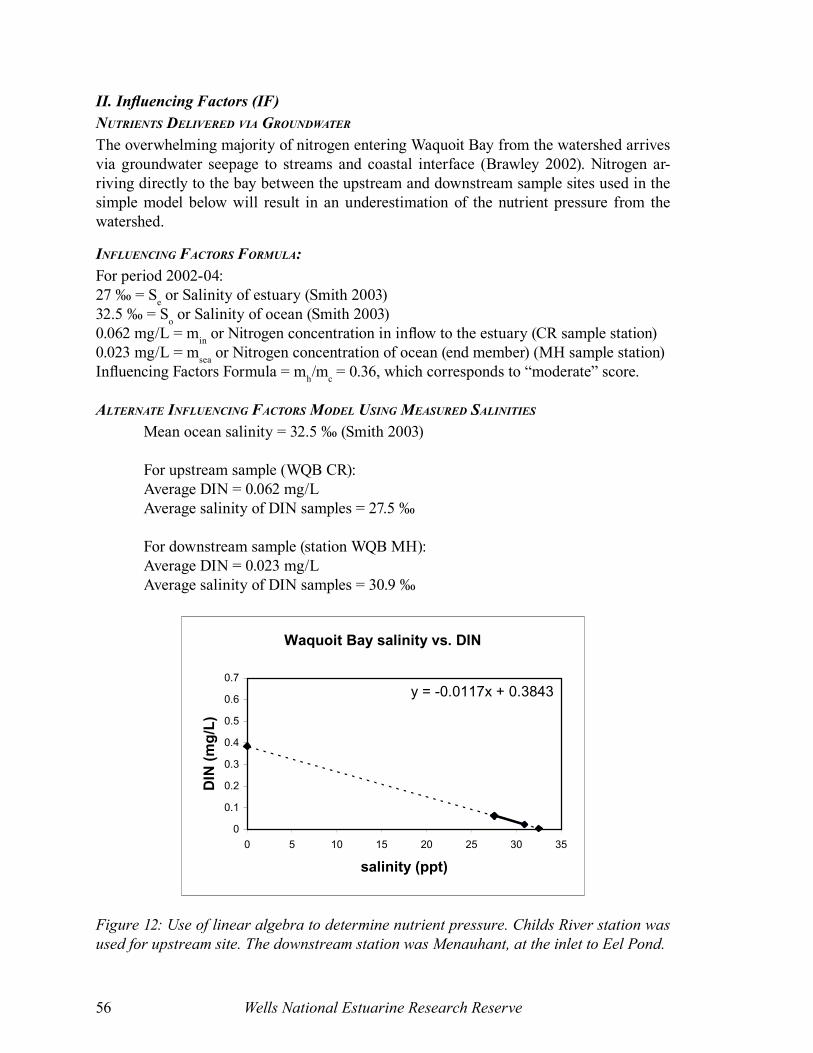
Wells National Estuarine Research Reserve56
II. Influencing Factors (IF)nutrients DelivereD via grounDWater
The overwhelming majority of nitrogen entering Waquoit Bay from the watershed arrives via groundwater seepage to streams and coastal interface (Brawley 2002). Nitrogen ar-riving directly to the bay between the upstream and downstream sample sites used in the simple model below will result in an underestimation of the nutrient pressure from the watershed.
inFluencing Factors Formula:For period 2002-04:27 ‰ = Se or Salinity of estuary (Smith 2003)32.5 ‰ = So or Salinity of ocean (Smith 2003)0.062 mg/L = min or Nitrogen concentration in inflow to the estuary (CR sample station)0.023 mg/L = msea or Nitrogen concentration of ocean (end member) (MH sample station)Influencing Factors Formula = mh/mc = 0.36, which corresponds to “moderate” score.
alternate inFluencing Factors moDel using measureD salinities
Mean ocean salinity = 32.5 ‰ (Smith 2003)
For upstream sample (WQB CR):Average DIN = 0.062 mg/LAverage salinity of DIN samples = 27.5 ‰
For downstream sample (station WQB MH):Average DIN = 0.023 mg/LAverage salinity of DIN samples = 30.9 ‰
Webhannet Estuary salinity vs. DIN
y = -0.0003x + 0.116
0
0.1
0.2
0.3
0.4
0.5
0.6
0.7
0 5 10 15 20 25 30 35
salinity (ppt)
DIN
(mg
/L)
Great Bay salinity vs. DIN
y = -0.0074x + 0.3055
0
0.1
0.2
0.3
0.4
0.5
0.6
0.7
0 5 10 15 20 25 30 35
salinity (ppt)
DIN
(mg
/L)
MBLR Estuary salinity vs. DIN
y = 0.0029x + 0.0954
0
0.1
0.2
0.3
0.4
0.5
0.6
0.7
0 10 20 30 40
salinity (ppt)
DIN
(mg
/L)
Waquoit Bay salinity vs. DIN
y = -0.0117x + 0.3843
0
0.1
0.2
0.3
0.4
0.5
0.6
0.7
0 5 10 15 20 25 30 35
salinity (ppt)
DIN
(mg
/L)
Figure 12: Use of linear algebra to determine nutrient pressure. Childs River station was used for upstream site. The downstream station was Menauhant, at the inlet to Eel Pond.
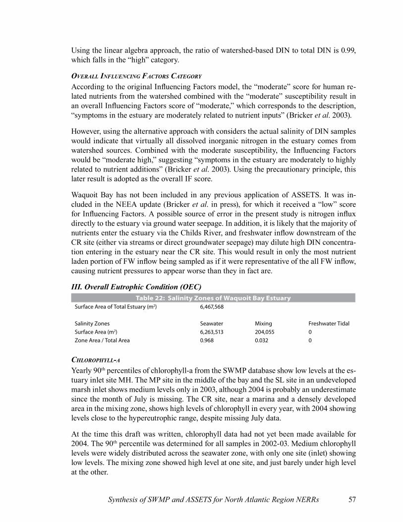
Synthesis of SWMP and ASSETS for North Atlantic Region NERRs 57
Using the linear algebra approach, the ratio of watershed-based DIN to total DIN is 0.99, which falls in the “high” category.
overall inFluencing Factors category
According to the original Influencing Factors model, the “moderate” score for human re-lated nutrients from the watershed combined with the “moderate” susceptibility result in an overall Influencing Factors score of “moderate,” which corresponds to the description, “symptoms in the estuary are moderately related to nutrient inputs” (Bricker et al. 2003).
However, using the alternative approach with considers the actual salinity of DIN samples would indicate that virtually all dissolved inorganic nitrogen in the estuary comes from watershed sources. Combined with the moderate susceptibility, the Influencing Factors would be “moderate high,” suggesting “symptoms in the estuary are moderately to highly related to nutrient additions” (Bricker et al. 2003). Using the precautionary principle, this later result is adopted as the overall IF score.
Waquoit Bay has not been included in any previous application of ASSETS. It was in-cluded in the NEEA update (Bricker et al. in press), for which it received a “low” score for Influencing Factors. A possible source of error in the present study is nitrogen influx directly to the estuary via ground water seepage. In addition, it is likely that the majority of nutrients enter the estuary via the Childs River, and freshwater inflow downstream of the CR site (either via streams or direct groundwater seepage) may dilute high DIN concentra-tion entering in the estuary near the CR site. This would result in only the most nutrient laden portion of FW inflow being sampled as if it were representative of the all FW inflow, causing nutrient pressures to appear worse than they in fact are.
III. Overall Eutrophic Condition (OEC)Table 22: Salinity Zones of Waquoit Bay Estuary
Surface Area of Total Estuary (m2) 6,467,568
Salinity Zones Seawater Mixing Freshwater TidalSurface Area (m2) 6,263,513 204,055 0Zone Area / Total Area 0.968 0.032 0
chloroPhyll-a
Yearly 90th percentiles of chlorophyll-a from the SWMP database show low levels at the es-tuary inlet site MH. The MP site in the middle of the bay and the SL site in an undeveloped marsh inlet shows medium levels only in 2003, although 2004 is probably an underestimate since the month of July is missing. The CR site, near a marina and a densely developed area in the mixing zone, shows high levels of chlorophyll in every year, with 2004 showing levels close to the hypereutrophic range, despite missing July data.
At the time this draft was written, chlorophyll data had not yet been made available for 2004. The 90th percentile was determined for all samples in 2002-03. Medium chlorophyll levels were widely distributed across the seawater zone, with only one site (inlet) showing low levels. The mixing zone showed high level at one site, and just barely under high level at the other.

Wells National Estuarine Research Reserve58
Given these data, chlorophyll concentration in the seawater zone is considered medium with high spatial distribution and episodic frequency. The mixing zone is considered high levels, high spatial distribution and periodic frequency. The overall expression value is moderate for Chl-a.
macroalgae
Waquoit Bay suffers from macroalgae at levels which dominate the bay and stifle submerged aquatic vegetation and other resources (Weidman, pers. comm.). Mats are persistent year round (although maximum frequency in the ASSETS decision table is “periodic,” defined as occurring predictably every year) in both the seawater and mixing zones, and at times are so thick that boaters cannot row through them. Dominant species are cladophora and gracilaria, with about 50% of the bay bottom covered with mostly cladophera. The overall expression level is “high” for macroalgae.
Figure 13: Salinity zones were updated using higher resolution coverage of the estuary and data from Waquoit Bay SWMP and NERR Baywatchers volunteer monitoring program.
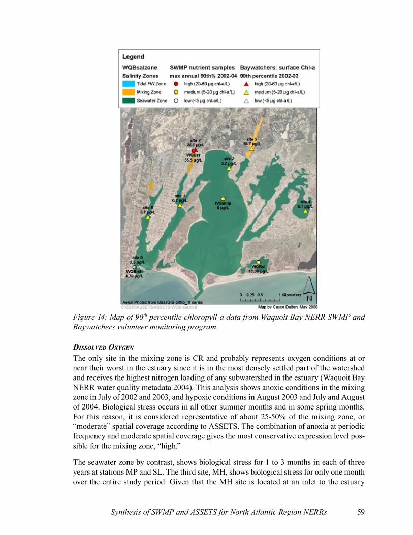
Synthesis of SWMP and ASSETS for North Atlantic Region NERRs 59
DissolveD oxygen
The only site in the mixing zone is CR and probably represents oxygen conditions at or near their worst in the estuary since it is in the most densely settled part of the watershed and receives the highest nitrogen loading of any subwatershed in the estuary (Waquoit Bay NERR water quality metadata 2004). This analysis shows anoxic conditions in the mixing zone in July of 2002 and 2003, and hypoxic conditions in August 2003 and July and August of 2004. Biological stress occurs in all other summer months and in some spring months. For this reason, it is considered representative of about 25-50% of the mixing zone, or “moderate” spatial coverage according to ASSETS. The combination of anoxia at periodic frequency and moderate spatial coverage gives the most conservative expression level pos-sible for the mixing zone, “high.”
The seawater zone by contrast, shows biological stress for 1 to 3 months in each of three years at stations MP and SL. The third site, MH, shows biological stress for only one month over the entire study period. Given that the MH site is located at an inlet to the estuary
Figure 14: Map of 90th percentile chloropyll-a data from Waquoit Bay NERR SWMP and Baywatchers volunteer monitoring program.
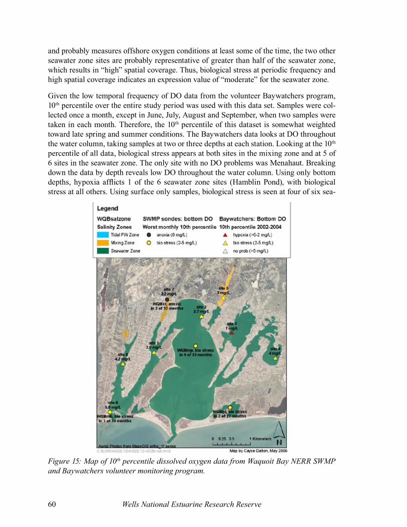
Wells National Estuarine Research Reserve60
and probably measures offshore oxygen conditions at least some of the time, the two other seawater zone sites are probably representative of greater than half of the seawater zone, which results in “high” spatial coverage. Thus, biological stress at periodic frequency and high spatial coverage indicates an expression value of “moderate” for the seawater zone.
Given the low temporal frequency of DO data from the volunteer Baywatchers program, 10th percentile over the entire study period was used with this data set. Samples were col-lected once a month, except in June, July, August and September, when two samples were taken in each month. Therefore, the 10th percentile of this dataset is somewhat weighted toward late spring and summer conditions. The Baywatchers data looks at DO throughout the water column, taking samples at two or three depths at each station. Looking at the 10th percentile of all data, biological stress appears at both sites in the mixing zone and at 5 of 6 sites in the seawater zone. The only site with no DO problems was Menahaut. Breaking down the data by depth reveals low DO throughout the water column. Using only bottom depths, hypoxia afflicts 1 of the 6 seawater zone sites (Hamblin Pond), with biological stress at all others. Using surface only samples, biological stress is seen at four of six sea-
Figure 15: Map of 10th percentile dissolved oxygen data from Waquoit Bay NERR SWMP and Baywatchers volunteer monitoring program.
Synthesis of SWMP and ASSETS for North Atlantic Region NERRs 61
water zone sites. Likewise, in the mixing zone, both sites show bottom biological stress and one site shows surface biological stress. Overall, the Baywatchers data do not show as bad a picture of DO in the mixing zone as the data sondes. However, they do indicate the same level as the sondes in the seawater zone. For this reason, the SWMP data provides the basis for the DO score. Taken together, the data indicate a high expression level for dissolved oxygen in the estuary as a whole over the study period.
The NEEA update indicated an overall low DO score for Waquoit Bay. That assessment, however, relied only on volunteer data (which were found in this study less indicative of problems) and the confidence is noted as speculative.
submergeD aquatic vegetation (eelgrass)Eelgrass was documented as rapidly declining in portions of the estuary in the decade prior to the study period, in part due to light limitation from heavy macroalgal blooms specifi-cally linked to increased nitrogen loading (Hauxwell et al. 2003). However, there has not been much change since about 2000 (Weidman, personal comm.). For this reason, the SAV score is considered moderate.
hazarDous or nuisance algal blooms (hab)Although nearby areas such as Marthas Vineyard, Buzzards Bay and Nausett have suffered from dinoflagelate blooms, Waquoit Bay has not (Weidman, personal communication). For this reason, it is scored as “no problem.”
overall eutroPhic conDition summary
Primary symptoms are “high.”Secondary symptoms are “high.”
Combining primary and secondary symptoms of eutrophication yields an overall “high” eutrophic condition for the study period. The ASSETS methodology describes this situa-tion as follows: “primary symptoms high and substantial secondary symptoms becoming more expressed, indicating potentially serious problems” (Bricker et al. 2003).
IV. Future Outlook (FO)Nutrients to Waquoit Bay estuary have steadily increased from the 1940’s to the present. This change is due from the 1970’s to the present primarily to wastewater increases, with atmospheric deposition decreasing and fertilizer trends generally flat (Valiela et al. 2002). Significant regional improvements in wastewater treatment have just been studied in recent years (Cape Cod Commission 2003), so results from such improvements are almost cer-tainly many years away.
Population and development are increasing in the region. Housing density increased 3.7 percent from 2000 to 2004 (Cape Cod Commission, 2005). Population is expected to in-crease 5-10 percent in the Cape Cod region between 2003-2008 (Crossett et al. 2004). All factors point to a likely increase in nutrient loads to the estuary. Combined with moderate pressure, this indicates a “worsen high” score, indicating that nutrient related symptoms are likely to substantially worsen.
Wells National Estuarine Research Reserve62
V. Overall Classification Grade (ASSETS)Pressure (IF): 2 = moderate highState (OEC): 1 = highResponse (FO): 1 = worsen highOverall: Bad
Due to significant differences in some components, especially in Influencing Factors and DO, the overall score is much different than the “moderate” reached in the NEEA update (Bricker et al. in press).
ReferencesBrawley J.W. 2002. Dynamic Modeling of Nutrient Inputs and Ecosystem Responses in the Waquoit Bay Estuarine System. Dissertation, U. Maryland, College Park.
Bricker S.D., D. Lipton, A. Mason, M. Dionne, D. Keeley, C. Krahforst, J. Latimer, J. Pennock. 2006. Improving methods and indicators for evaluating coastal water eutrophica-tion: a pilot study in the Gulf of Maine. Report to NOAA-CICEET. 66p.
Cambareri, T.C., and E. M. Eichner. 1998. Watershed delineation and ground water dis-charge to a coastal embayment. Ground Water 36 (4): 626-634.
Cape Cod Commission, Water Resources Office, Barnstable County. 2003. Cape cod Comprehensive Regional Wastewater Management Strategy Development Project.http://www.capecodcommission.org/data/CapeTrends-Housing090805.pdf
Cape Cod Commission. 2005. Housing Growth, parts I & II. Cape Trend Update. Accessed 22 May 2006.http://www.capecodcommission.org/data/CapeTrends-Housing090805.pdf http://www.capecodcommission.org/data/CapeTrends-Housing101305.pdf
Carmichael, R. H., B. Annett, I. Valiela. 2004. Nitrogen Loading to Pleasant Bay, Cape Cod: Application of Models and Stable Isotopes to Detect Incipient Nutrient Enrichment of Estuaries. Marine Pollution Bulletin 48:137-143.
Cole, M. L., I. Valiela, K. D. Kroeger, G. L. Tomasky, J. Cebrian, C. Wigand, R. A. McKinney, S. P. Grady, M. H. Carvalho da Silva. 2004. Assessment of a d15N Isotopic Method to Indicate Anthropogenic Eutrophication in Aquatic Ecosystems. Journal of Environmental Quality. 33:124-132.
Crossett, K. M., T. J. Culliton, P.C. Wiley, T. R. Goodspeed. 2004. Population Trends Along the Coastal United States: 1980-2008. National Oceanic and Atmospheric Administration, National Ocean Service, Management and Budget Office, Special Projects. Coastal Trends Report Series.
Hauxwell, J., J. Cebrián, I. Valiela. 2003. Eelgrass Zostera marina loss in temperate estuar-ies: relationship to land-derived nitrogen loads and effect of light limitation imposed by algae. Marine Ecology Progress. 247:59-73.
Synthesis of SWMP and ASSETS for North Atlantic Region NERRs 63
Howes B., S.W. Kelley, J.S. Ramsey, R. Samimy, D. Schlezinger, T. Ruthven, E. Eichner 2005. Linked Watershed-Embayment Model to Determine Critical Nitrogen Loading Thresholds for the Quashnet River, Hamblin Pond, and Jehu Pond, in the Waquoit Bay System in the Towns of Mashpee and Falmouth, Massachusetts. Massachusetts Estuaries Project, Massachusetts Department of Environmental Protection. Boston, MA.
Massachusetts Executive Office of Environmental Affairs (MA EOEA). February 2003. EOEA Cape Cod Watershed Assessment and Action Plan. http://www.mass.gov/envir/water/publications/CapeCod/SubwatershedFactSheets/WaquoitBay.pdf
Smith, S.V. 2003. Preliminary NOAA estuarine typology database.
Valiela I., J.L. Bowen. 2002. Nitrogen Sources to Watershed and Estuaries: Role of Land Cove Mosaics and Losses within Watersheds. Environmental Pollution 118:239-248.
Wright-Pierce. 2004. Enhancing Wastewater Management on Cape Cod: Planning, Administrative, and Legal Tools. Report to Barnstable County, Wastewater Implementation Committee (WIC)http://www.capecodcommission.org/water/WastewaterToolsReport/WWToolsRept.pdf
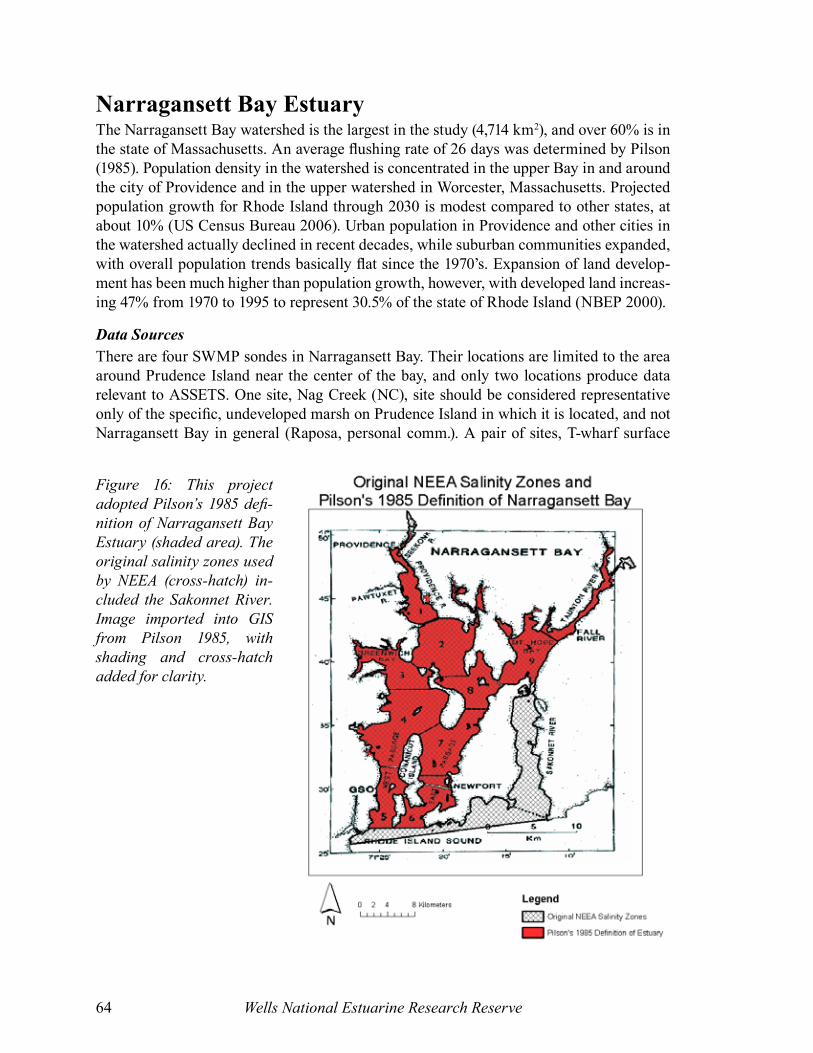
Wells National Estuarine Research Reserve64
Narragansett Bay EstuaryThe Narragansett Bay watershed is the largest in the study (4,714 km2), and over 60% is in the state of Massachusetts. An average flushing rate of 26 days was determined by Pilson (1985). Population density in the watershed is concentrated in the upper Bay in and around the city of Providence and in the upper watershed in Worcester, Massachusetts. Projected population growth for Rhode Island through 2030 is modest compared to other states, at about 10% (US Census Bureau 2006). Urban population in Providence and other cities in the watershed actually declined in recent decades, while suburban communities expanded, with overall population trends basically flat since the 1970’s. Expansion of land develop-ment has been much higher than population growth, however, with developed land increas-ing 47% from 1970 to 1995 to represent 30.5% of the state of Rhode Island (NBEP 2000).
Data SourcesThere are four SWMP sondes in Narragansett Bay. Their locations are limited to the area around Prudence Island near the center of the bay, and only two locations produce data relevant to ASSETS. One site, Nag Creek (NC), site should be considered representative only of the specific, undeveloped marsh on Prudence Island in which it is located, and not Narragansett Bay in general (Raposa, personal comm.). A pair of sites, T-wharf surface
Figure 16: This project adopted Pilson’s 1985 defi-nition of Narragansett Bay Estuary (shaded area). The original salinity zones used by NEEA (cross-hatch) in-cluded the Sakonnet River. Image imported into GIS from Pilson 1985, with shading and cross-hatch added for clarity.

Synthesis of SWMP and ASSETS for North Atlantic Region NERRs 65
(TS) and bottom (TB) is unlike most SWMP sample stations in that both a surface and bottom sonde are deployed. For ASSETS at T-wharf, the bottom sonde provides relevant DO information, while the surface sonde provides relevant salinity and chlorophyll data. For these reasons and the fact that the estuary is large with several significant freshwater tributaries, the SWMP sites alone would provide an extremely limited view of eutrophica-tion in this estuary.
Fortunately, there are many additional sample sondes of the same type as used by SWMP deployed in the bay attached to buoys or docks. Data collection is managed by different organizations, and is collected and distributed under the “Bay Window” umbrella program. This program is still being developed and expanded, so for the study period data availabil-ity is limited mostly to 2004, the period of data collection is seasonal and varies from site to site in length, QA/QC does not seem equal to the thorough review SWMP undergoes, and metadata does not appear to be available for most data files. Nonetheless, these sondes pro-vide some level of information in the same format and with the same equipment as SWMP, and seems to be expanding and improving in quality on a year to year basis. It should be a worthwhile source of data for future ASSETS replications, and has the potential for auto-mated integration with the SWMP database since formats are so similar.
For this report, only 2004 Bay Window data are considered, although a few files are spo-radically available for earlier years. All but one sonde is part of a surface-bottom pair at the same location. Considering when possible bottom sondes for dissolved oxygen and surface sondes for chlorophyll-a, there are twelve sondes at seven locations in addition to SWMP stations that are monitored.
I. SusceptibilityTable 23: Dilution Potential of Narragansett Bay
Vertical Stratification Minor Pilson 1985, Nixon 1995Volume of Estuary (m3) 2.72 X 10⁹ Pilson 1985Volume of Estuary (ft3) 9.62 X 10¹⁰
Vol of FW Fraction Not NeededDilution Value (1/volume ft3) 1.04 X 10⁻¹¹
Dilution Potential ModerateTable 24: Flushing Potential of Narragansett Bay
Tidal Range 1.9-1.1 m (6.2-3.6 ft) Pilson 1985Tidal Range Category MesoFW Inflow (m3/day) 9,072,000 Pilson 1985FW Inflow (ft3/day) 3.2 X 10¹⁰
FW Inflow / Estuary Volume 3.3 X 10⁻³
FW Inflow / Est Vol Catagory SmallFlushing Potential LowSusceptibility High
This is in contrast to moderate susceptibility in the most recent application of ASSETS, which found high dilution potential and moderate susceptibility (Bricker et al. 2006). The current study excludes the Sakonnet River and redraws the southern border slightly in order
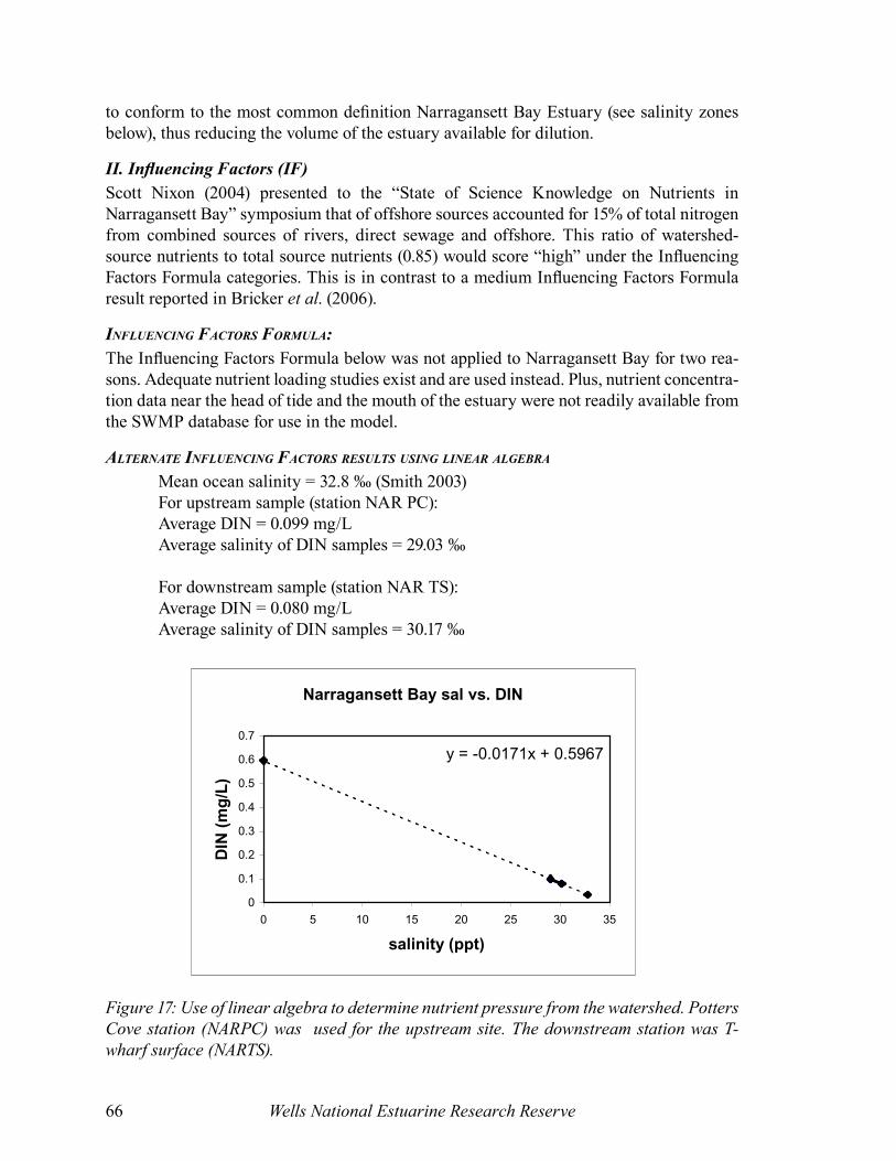
Wells National Estuarine Research Reserve66
to conform to the most common definition Narragansett Bay Estuary (see salinity zones below), thus reducing the volume of the estuary available for dilution.
II. Influencing Factors (IF)Scott Nixon (2004) presented to the “State of Science Knowledge on Nutrients in Narragansett Bay” symposium that of offshore sources accounted for 15% of total nitrogen from combined sources of rivers, direct sewage and offshore. This ratio of watershed-source nutrients to total source nutrients (0.85) would score “high” under the Influencing Factors Formula categories. This is in contrast to a medium Influencing Factors Formula result reported in Bricker et al. (2006).
inFluencing Factors Formula:The Influencing Factors Formula below was not applied to Narragansett Bay for two rea-sons. Adequate nutrient loading studies exist and are used instead. Plus, nutrient concentra-tion data near the head of tide and the mouth of the estuary were not readily available from the SWMP database for use in the model.
alternate inFluencing Factors results using linear algebra
Mean ocean salinity = 32.8 ‰ (Smith 2003)For upstream sample (station NAR PC):Average DIN = 0.099 mg/LAverage salinity of DIN samples = 29.03 ‰
For downstream sample (station NAR TS):Average DIN = 0.080 mg/LAverage salinity of DIN samples = 30.17 ‰
Narragansett Bay sal vs. DIN
y = -0.0171x + 0.5967
0
0.1
0.2
0.3
0.4
0.5
0.6
0.7
0 5 10 15 20 25 30 35
salinity (ppt)
DIN
(mg
/L)
Figure 17: Use of linear algebra to determine nutrient pressure from the watershed. Potters Cove station (NARPC) was used for the upstream site. The downstream station was T-wharf surface (NARTS).

Synthesis of SWMP and ASSETS for North Atlantic Region NERRs 67
Using the above method results in a ratio of watershed to offshore DIN of 0.94, correspond-ing to a “high” level for Influencing Factors Formula, the same category using Nixon’s figures above.
overall inFluencing Factors category
The high score for human related nutrients from the watershed combined with the high susceptibility result in an overall Influencing Factors score of “high,” which corresponds to the description, “symptoms in the estuary are probably closely related to nutrient addi-tions” (Bricker et al. 2003).
III. Overall Eutrophic Condition (OEC)The definition of Narragansett Bay Estuary used in the calculation of salinity zones presented by Michael Pilson in 1985, by Scott Nixon in 1995, and by Christopher Deacutis (personal comm. 2005). Previous applications of NEEA and ASSETS included the Sakonnet River, which has been excluded in the present and prior definitions since it is best characterized as a marine embayment with extremely limited exchange with estuarine waters.
salinity zones
The salinity zone delineations used in previous NEEA / ASSETS studies were compared to salinity data from each sample station. Since no conflict was noted, the previous delinea-tions were maintained.
Table 25: Salinity Zones of Narragansett Bay EstuarySurface Area of Total Estuary (m2) 326,355,109
Salinity Zones Seawater Mixing Freshwater TidalSurface Area (m2) 282,833,314 42,434,154 1,087,641Zone Area / Total Area 0.867 0.130 0.003
chloroPhyll-a
Yearly 90th percentiles of chlorophyll-a from the SWMP database show medium levels on an episodic basis. The 90th percentile of all data during the study period (2002-2004) at each site indicates low levels. These data come from grab samples analyzed by fluores-cence in the lab.
The Bay Window program appears to measure via an optical probe attached to a YSI 6000 or 6600 data sonde. This in vivo method is considered fully accurate only when calibrated to a phytoplankton suspension of known chlorophyll-a concentration obtained by an ex-tractive process in the lab (YSI Incorporated, undated). Documentation of such calibration is absent in the Bay Window chlorophyll data, and are assumed to be uncalibrated. The data can nonetheless still be used as an approximation of chlorophyll levels, providing at least some data where no other records exist. Looking at the data with this understanding, the yearly 90th percentiles from the Bay Window program indicate four locations at the borderline between medium and high levels (between 19.5 and 21.8 μg chl-a/L). One site, Bullocks Reach, is clearly in the high range at 29.8 μg chl-a/L. Three sites (Phillipsdale Landing, GSO Dock and Popasquash Point) are clearly in the medium range. Since these
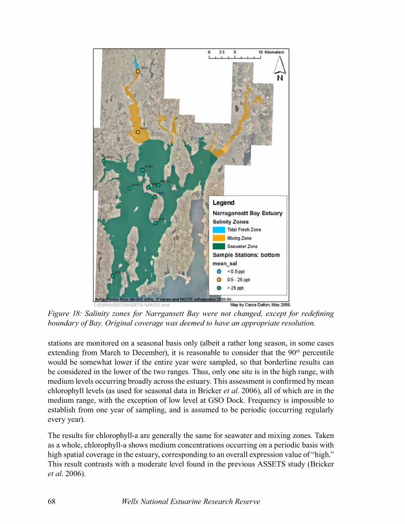
Wells National Estuarine Research Reserve68
stations are monitored on a seasonal basis only (albeit a rather long season, in some cases extending from March to December), it is reasonable to consider that the 90th percentile would be somewhat lower if the entire year were sampled, so that borderline results can be considered in the lower of the two ranges. Thus, only one site is in the high range, with medium levels occurring broadly across the estuary. This assessment is confirmed by mean chlorophyll levels (as used for seasonal data in Bricker et al. 2006), all of which are in the medium range, with the exception of low level at GSO Dock. Frequency is impossible to establish from one year of sampling, and is assumed to be periodic (occurring regularly every year).
The results for chlorophyll-a are generally the same for seawater and mixing zones. Taken as a whole, chlorophyll-a shows medium concentrations occurring on a periodic basis with high spatial coverage in the estuary, corresponding to an overall expression value of “high.” This result contrasts with a moderate level found in the previous ASSETS study (Bricker et al. 2006).
Figure 18: Salinity zones for Narrgansett Bay were not changed, except for redefining boundary of Bay. Original coverage was deemed to have an appropriate resolution.

Synthesis of SWMP and ASSETS for North Atlantic Region NERRs 69
macroalgae
Macroalgae appear not to have been extensively monitored during the study period, and a data gap for this symptom is acknowledged (Raposa, pers. comm.). Nonetheless, anecdotal reports indicate heavy presence of sea lettuce (Ulva lactuca) in the mixing zone. Portions of the seawater zone also experience nuisance macroalgal blooms, in general worse on the western side of the bay, and particularly severe in Greenwich Bay where they appear to remain due to inadequate flushing (Deacutis, personal comm.). Rhode Island Sea Grant (2005) and Department of Environmental Management (RISG 2005) have regularly ob-served thick macroalgae blooms in the upper parts of the bay. Given the fact that macroalgae are a problem for the two biggest zones of the estuary, and that these problems appear every year, the expression level for macroalgae is “high.” Taking the average of chlorophyll-a and macroalgae scores, the overall expression level for primary symptoms is “high.”
Figure 19: Chlorophyll-a data for Narrgansett Bay were provided by Narragansett Bay NERR, Narragansett Bay Commission, University of Rhode Island Graduate School of Oceanography, and RI DEM.

Wells National Estuarine Research Reserve70
DissolveD oxygen
In the seawater zone, levels from anoxic to no problem were revealed. The anoxic read-ings occurred at the Nag Creek site, which as mentioned earlier should not be considered as representative of Narragansett Bay generally. Hypoxia occurs on an episodic basis at Potters Cove (2 of 3 years), and only one month of the 2004 data available for Greenwich Bay. Many areas in Greenwich Bay were documented as experiencing anoxia in the mid 1990’s (Granger, et al. 2000).
Levels of biological stress occurred at two stations in the middle part of the Narragansett Bay, but not at the station nearest the mouth. Based on the sonde data alone, it would ap-pear that hypoxia at a low spatial coverage (10-25% of estuary) occurs on a periodic basis. However, these data do not seem to capture the reports of anoxia in upper parts of the bay of the type that led to the massive fish kill in Greenwich Bay in August 2003 (RIDEM 2003). Regardless, under either set of conditions—anoxic conditions at low spatial coverage (less
Figure 20: Dissolved oxygen from available sondes during the study period for Narragansett Bay. Data comes from Narragansett Bay NERR, Narragansett Bay Commission, University of Rhode Island Graduate School of Oceanography, and RI DEM.

Synthesis of SWMP and ASSETS for North Atlantic Region NERRs 71
than 25% of the zone) and episodic frequency, or hypoxia at low coverage (10-25%) and periodic frequency—the resulting score based on the ASSETS decision table is “low” for the seawater zone.
There are only two sondes in the mixing zone during the study period, both in the Providence River. The further upstream station, near the freshwater tidal zone interface, showed peri-ods of anoxia, while the lower one showed biological stress levels. The most conservative score under the precautionary principle for conditions in the mixing zone is “moderate,” associated with biological stress levels at a high spatial coverage and periodic frequency.
The “Insomniacs” dissolved oxygen data, collected on six summer nights in 2002 and 2003 was analyzed and presented in a previous ASSETS study (Bricker et al. 2006). That set of data suggests a moderate score for dissolved oxygen based on moderate concentration, moderate spatial coverage and periodic frequency. Further evidence for more serious DO depletion includes fish kills in 1999 and 2003. Using the precautionary principle, the lower score is adopted here, so that DO is considered moderate.
The stark contrast between the entirely benign picture painted by the data sonde 10th per-centile DO with the ASSETS decision tables versus the history of fish kills is a signal that the ASSETS criteria for DO should be carefully examined to ensure they are appropriate for use with high frequency, low spatial resolution data provided by SWMP. The precau-tionary principle in determining the DO score bears repeating in this case. Specifically, a probable weakness of ASSETS is the aggregation of the DO score for the estuary as a whole, so that severe but spatially limited problems are “averaged out” by large areas with no problems, as in this case. A potential solution would be to weight more heavily anoxia at very low to moderate spatial coverage (this combination currently results in “low” score if frequency is episodic).
submergeD aquatic vegetation (eelgrass)Eelgrass beds in Narragansett Bay have suffered major losses from the 1800’s to recent decades. Current beds total about 100 acres. The most recent survey was done in 1995, so near term changes are not known, but are not expected to have changed significantly due to eutrophication, since nutrient levels have remained about the same (Deacutis, personal comm.). Based on this information, SAV is considered not to have changed during the study period, with a consequent “low” score for the estuary.
hazarDous or nuisance algal blooms (hab)Although the potential exists for HAB’s in Narragansett Bay, with episodes of brown tides occurring in the mid 1980’s, they have not been a problem in recent years. When they do occur, they tend to originate in the Gulf of Maine and advect into the bay (Deacutis, personal comm.). For this reason, they are scored as “no problem.”
overall eutroPhic conDitions summary
Primary symptoms are “high.”Secondary symptoms are “moderate.”
Wells National Estuarine Research Reserve72
Combining primary and secondary symptoms of eutrophication yields an overall “moder-ate high” eutrophic condition for the study period. The ASSETS methodology describes this situation as follows: “Primary symptoms high and substantial secondary symptoms becoming expressed, indicating potentially serious problems.” (Bricker et al. 2003).
IV. Future Outlook (FO)Population growth has been basically flat over the past several decades while land con-sumption has increase substantially (NBEP 2005). Nitrogen inputs via tributaries have not significantly increased, while phosphorous inputs have declined (Nixon, et al. 2005). Population is expected to increase over the coming years (Crosset et al. 2004; US Census Bureau 2006), but wastewater treatment is also expected to improve as nitrogen removal processes are implemented (Bricker et al. 2006). On balance, nutrient pressure is not ex-pected to change.
Combined with the high susceptibility, flat nutrient trends would indicate a “no change” score for Future Outlook, which corresponds to the statement “nutrient related symptoms will most likely remain unchanged.”
V. Overall Classification Grade (ASSETS)Pressure (IF): 1 = highState (OEC): 2 = moderate highResponse (FO): 3 = no changeOverall: bad
The overall score is slightly worse than that reached by the Gulf of Maine Pilot Study (Bricker et al. 2006). The primary differences are a worse result here for dilution potential, which worsened susceptibility, and a worse Influencing Factors Formula result which wors-ened Influencing Factors. An additional difference is a better score here for chlorophyll-a. The result is the same as the NEEA Update (Bricker et al. in press).
ReferencesBricker S.B., C.G. Clement, D. E. Pirhalla, S.P. Orlando, and D.R.G. Farrow. 1999. National Estuarine Eutrophication Assessment. Effects of Nutrient Enrichment in the Nation’s Estuaries. NOAA, National Ocean Service, Special Projects Office and National Centers for Coastal Ocean Science, Silver Spring.
Bricker, S.B., J.G. Ferreira, and T. Simas. 2003. An Integrated Methodology for Assessment of Estuarine Trophic Status. Ecol. Modelling 169: 39-60.
Bricker S.B., D. Lipton, A. Mason, M. Dionne, D. Keeley, C. Krahforst, J. Latimer, J. Pennock. 2006. Improving methods and indicators for evaluating coastal water eutrophica-tion: a pilot study in the Gulf of Maine. Report to NOAA-CICEET. 66p.
Granger, S., M Brush, B. Buckley, M. Traber, M. Richardson, and S.W. Nixon. 2000. An Assessment of Eutrophication in Greenwich Bay. Paper No. 1 in: M. Schwartz (ed.) Restoring Water Quality in Greenwich Bay: A Whitepaper Series. Rhode Island Sea Grant, Narragansett, R.I. 20pp.
Synthesis of SWMP and ASSETS for North Atlantic Region NERRs 73
Nixon, S. 1995. An Assessment of the Annual Mass Balance of Carbon, Nitrogen and Phosphorus in Narragansett Bay. Biogeochemistry. 31:15-61.
Nixon, S., 2004. The Risk of Hypoxia in Narragansett Bay: A Synthesis of Available Data. Presented at State of Science Knowledge on Nutrients in Narragansett Bay. May 19,2005. http://seagrantadm.gso.uri.edu/04_sci_symp_web/1_Nixon_KEY.ppt
Nixon, S., B Buckley, S. Granger, L. Harris, A. Oczkowski, L. Cole, and R. Fulweiler. 2005. Anthropogenic Nutrient Inputs to Narragansett Bay: A twenty five year perspec-tive. Report to Narragansett Bay Commission and Rhode Island Sea Grant. Grad School Oceanography, U Rhode Island.
Pilson, M.E.Q. 1985. On the Residence Time of Water in Narragansett Bay. Estuaries, 8:2-14.
Rhode Island Department of Environmental Management (RIDEM). 2003. Greenwich Bay Fish Kill – August 2003: Causes, Impacts and Responses.http://www.dem.ri.gov/pubs/fishkill.pdf
Rhode Island Sea Grant (RISG) 2005. State of Science on Nutrients in Narragansett Bay: Findings and Recommendations from the Rhode Island Sea Grant 2004 Science Symposium. Eds: Carey, D., A. Desbonnet, A.B. Colt, B.A. Costa-Pierce.http://seagrant.gso.uri.edu/research/RISG_Nutrient_Symp_Synthesis.pdf
Smith, S.V. 2003. Preliminary NOAA estuarine typology database.
US Census Bureau. 2006. Florida, California and Texas to Dominate Future Population Growth, Census Bureau Reports.http://www.census.gov/Press-Release/www/releases/archives/population/004704.html
YSI Incorporated. Undated, ca. 2002. 6-Series Environmental Monitoring Systems Manual, Appendix I Chlorophyll Measurements. Yellow Springs, Ohio.
Wells National Estuarine Research Reserve74
Old Woman CreekOld Woman Creek NERR is located in a agricultural watershed in Ohio near the south-ernmost point of Lake Erie. The mouth of the stream is a drowned river channel in which tributary and offshore waters sometimes mix, creating a freshwater estuary. The dynamics of this estuary are distinct in many ways from the marine estuaries presented above, and the appropriateness of the ASSETS methodology to determining its eutrophic status is ad-mittedly unproven. The following represents a first approximation at applying ASSETS to a Great Lakes estuary, one which may be used as a starting point for future development.
Besides the obvious lack of a strong salinity gradient, there are several other essential hydrological and morphological differences between Old Woman Creek and the marine estuaries. First, mixing of offshore and tributary waters in the estuary does not follow a semi-diurnal pattern. In fact, a barrier beach often forms due to littoral drift and wave action which prevents mixing of offshore and estuarine waters for months at a time. This barrier is breached when high water levels and storm runoff undercut and then overtop the barrier beach, or more rarely from a strong north or northwest wind which causes lake water to crest the beach, creating an inlet. Once the mouth is opened, wind-driven seiche cause estuary water levels to vary. These seiche events are similar to tides, with a 10-14 hour cycle, although their timing is unpredictable. (Herndendorf et al. 2006; Klarer, pers. comm.).
An important dynamic absent from marine estuaries is the significant decadal-scale varia-tion of offshore (lake) water level. Since 1999, the lowering of Lake Erie has increased the amount of mudflats in the estuary, and caused changes in size, location and dominant spe-cies of aquatic macrophyte zones (Herndendorf et al. 2006). With this constantly shifting ecological backdrop, it may be more difficult to quantify trends in eutrophication, since spatial coverage of many symptoms may be greatly altered by water depth, making spa-tially-based comparisons from year to year difficult.
Old Woman Creek is considered strongly eutrophic. Herndendorf et al. (2006) cites the strong summertime diurnal swings in dissolved oxygen and pH as evidence of extremely high primary production typical of a hypertrophic wetland. Photosynthesis during the day produces more oxygen than can be respired within the estuary or diffused to the atmo-sphere, supersaturating the water with oxygen. At the same time, uptake of free carbon dioxide from the water by primary producers outpaces diffusion into the water from the atmosphere increasing pH. At night, respiration drives down oxygen levels and releases carbon dioxide in the water, reversing the two trends.
Data SourcesThere are four SWMP sondes deployed during the ice-free season (early March – mid December) at Old Woman Creek NERR. One sample station is near the mouth of the estu-ary (WM), one in the lower reaches (OL), one in the upstream reaches (SU) and one just upstream from the last riffle area in the stream before waters enter the estuary (BR). These four sites offer the potential for examining gradients along the estuary, however, the fact that the estuary is frequently sealed off from Lake Erie means that the gradient may not always represent the relationship of offshore waters to those from the watershed.

Synthesis of SWMP and ASSETS for North Atlantic Region NERRs 75
I. SusceptibilityDilution potential was determined using the same metrics as the marine estuaries. A recent study by Krieger (2001) conducted over a three year period determined that the volume of the estuary varied from around 360,000 to 600,000 m3. An order of magnitude estimate of 500,000 m3 was used for the purposes determining dilution potential here. Mitsch et al. (1989) determined tributary inflow to the estuary to be 0.18 m3/s. Evidence has been found for significant mixing of Lake Erie waters with riverine and estuarine waters along its shore (Herndendorf et al. 2006). Using these inputs and the ASSETS parameters, dilution potential is decidedly low.
Flushing potential was determined heuristically as follows. Tidal range on Lake Erie is on the order of magnitude of 0.1 – 0.2 m (Herndendorf et al. 2006). More significant flushing events do occasionally occur, but they depend on periods when the mouth of the estuary is open to Lake Erie. During Krieger’s (2001) three year study period, a barrier beach closed the mouth of the estuary from one fourth to one half of the time, during which surface water flow to the lake was essentially zero. This barrier beach tended to be created by heavy surf on Lake Erie, while a combination of high water in the estuary and storm runoff events tend to open it. Since water flows are lower in the summer and autumn, the estu-ary is typically closed during these seasons (Krieger 2001). When the estuary is open to offshore waters, northern winds occasionally create seiche events in which offshore water moves upstream into the estuary generating mixing (Whyte 1996). Based solely on the low tidal range and occasional nature of mixing events, flushing potential was assessed as low. A more nuanced assessment might assess separately periods when the mouth was open and when it was closed. Given the combination of low flushing and low dilution potentials, the susceptibility of Old Woman Creek is determined to be high.
II. Influencing Factors (IF)The Influencing Factors concept in ASSETS focuses on the ratio of nutrients coming from the watershed to the total amount of nutrients (offshore and watershed sources combined) in the estuary. Application of the two formulas used in the saltwater estuaries above to a freshwater estuary presents several challenges. The most obvious is how to estimate dilu-tion of tributary inflow to offshore waters within the estuary in the absence of a strong salinity gradient. It appears that specific conductivity could in fact be used for this purpose if both offshore and tributary values were known with greater precision than that delivered by the water quality component of SWMP (YSI probes). OWC nutrient data under SWMP does in fact include specific conductivity of each nutrient sample at what would appear to be an appropriate level of precision to estimate dilution, both within the estuary and just offshore. However, there are other serious limitations to the application of the IF formula, and the availability of loading values made such an attempt unnecessary.
Even if the IF formula could be applied, its underlying assumption of conservation of nu-trients within the estuary is considerably compromised in the case of Old Woman Creek. Studies have determined that between 35 and 80% of biologically important nutrients are retained or transformed within the estuary. Specifically, comparing outflow from the estu-ary relative to inflow, soluble reactive phosphorous was measured as 77% lower, nitrate was 42% lower and silicate was 49% lower (Herndendorf et al. 2006). Krieger (2001) found

Wells National Estuarine Research Reserve76
that total nitrogen load was 14% lower in outflow relative to inflow (with ammonium actu-ally increasing). The simple dilution model incorporated in the IF formulas fails to account for these transformations.
Further complicating this question in the case of Old Woman Creek is the alternating na-ture of the estuary. Sometimes, a barrier beach seals out offshore water during low flow periods. The estuary is opened again to offshore influences when high water and storm runoff combine to breech this barrier. When the beach is closed, essentially all nutrients in the estuary come from watershed sources, translating at least during these periods into an IF of 1. During the open periods, however, the influx of offshore water and nutrients is somewhat irregular, and considered less frequent than in semi-diurnal tidal estuaries.
Finally, which nutrient(s) should be analyzed? The typical assumption in freshwater systems is that phosphorus is the limiting nutrient. However, in the case of Old Woman Creek there is conflicting evidence in this regard. The N:P ratio is 29.67 would indicate phosphorus limitation (Heath 1992), whereas studies of phosphatase specific activity do not indicate P-limitation (Heath 1987), and some evidence was found to indicate occasional N-limitation (Heath 1987, 1992).
loaDing
Given the difficulties in applying the IF formulas to Old Woman Creek, the scientific lit-erature is an alternate source for determining the relative contributions from the watershed and offshore waters. A total phosphorus (TP) mass balance is presented in Mitsch et al. (1989). Here, TP from the watershed greatly overwhelms that from offshore (2.2 to 0.009 mg-P/m2-day). Krieger (pers. comm.) points out that this loading was calculated under drought conditions, and is probably not typical. Nonetheless, the ratio is so overwhelming that it provides some basis for an IF of “high” with vastly more TP in the estuary coming from the watershed than offshore.
inFluencing Factors
The “high” score for human related nutrients from the watershed combined with the “high” susceptibility result in an overall Influencing Factors score of “high,” which corresponds to the description, “symptoms in the estuary are probably closely related to nutrient addi-tions” (Bricker et al. 2003).
III. Overall Eutrophic Condition (OEC)salinity zones
While it may be possible to use salinity (specific conductivity) in Great Lakes estuaries to create an analogous system of zones, it would require measurements that exceeds the precision of the water quality component of SWMP as currently deployed. Furthermore, the irregularity of offshore inundations of the estuary would greatly limit the value of such zonation. In any case, determining such a method was beyond the scope of this project and data were assessed and weighted across the estuary as if pertaining to one zone. Where significant differences were noted across the estuary, data were weighted heuristically.

Synthesis of SWMP and ASSETS for North Atlantic Region NERRs 77
chloroPhyll-a
Old Woman Creek’s dominant primary producer has been described both as phytoplankton and macrophytes. This apparent contradiction is explained as accurate for different time periods, and provides an indication of the ecological variability in the estuary (Herndendorf et al. 2006). Observations during and after storm events lend support to the idea that phy-toplankton are the fundamental primary producers. After large influxes of stormwater, the summertime pattern of diurnal swings in dissolved oxygen and pH were significantly dampened, only to return after about a week. This pattern suggest that the storm washed away existing phytoplankton populations, which then slowly reestablished themselves (Herndendorf et al. 2006).
Yearly 90th percentiles of chlorophyll-a from the SWMP database show high levels at three of four sites (all but BR). Two of these sites show high levels during all three years (WM and OL). Considering high concentrations, high spatial coverage and periodic frequency the expression value for chlorophyll-a is “high.”
macroalgae
Old Woman Creek does not have any macroalgae, although filamentous (and rarely Blue-Green) algae sometimes grow to macroscopic proportions (Klarer, pers. comm.). Given the uncertainty of the appropriateness of this measure to a freshwater estuary compared to the relatively universal value of chlorophyll-a, this symptom is excluded from the ASSETS analysis of Old Woman Creek.
DissolveD oxygen
Dissolved oxygen is perhaps the most universal measure applied by ASSETS. Its value as a measure of eutrophication can be considered relatively independent of the saltwater or freshwater nature of the estuary under investigation. Mitch and Reeder in Mitch et al. (1989) noted dramatic diurnal swings in dissolved oxygen at Old Woman Creek during the summer (from 2 to 14 mg/L), driven by estuary metabolism in which photosynthesis super-saturates the water during the day and respiration rapidly depletes it at night. (Under such a regime, the authors state it would be “unwise” to think the estuary could ever support a diverse fish population.)
Using the monthly 10th percentile for dissolved oxygen, given its high temporal resolution, reveals that the lowest DO levels over the study period were anoxic (0.1 mg/L, which is below the level of accuracy of +/- 0.2 mg/L of the DO probe and to be conservative is con-sidered to indicate possible anoxic conditions). However, this level of DO appears in only one of the 115 monthly data sets of the study period (site SU, June 2002). Using low spatial coverage, episodic frequency and anoxic conditions results in a “low” DO expression value. However, hypoxic conditions occur at all four sites in two of three years. Using hypoxia at high spatial coverage and episodic frequency results in “moderate” DO expression value. Using the precautionary principle, this “moderate” value for DO is adopted.
submergeD aquatic vegetation
The submerged aquatic vegetation in the estuary is fairly minor component of the macro-phyte community. There do occur scattered but dense beds of Ceratophyllum demersum

Wells National Estuarine Research Reserve78
or Potamogeton pectinatus. In 2006, these beds are much more extensive than in previous years, but still remain a minority part of the aquatic macrophyte community (Klarer, pers. comm.).
Freshwater estuaries such as Old Woman Creek have a more diverse community of aquatic vegetation than marine estuaries. Seasonal and long term changes in vegetation are con-tinuous, and causes include changes in Lake Erie’s water level, and periodic breeches in the barrier beach which drains the estuary (Whyte 1996). Given the continuous nature of these changes and the fact that many causes do not relate to eutrophication, it is unlikely that spatial coverage of submerged vegetation would be a suitable indicator of eutrophic condition in the estuary and is excluded in the case of Old Woman Creek.
hazarDous or nuisance algal blooms (hab)In the Great Lakes, potentially toxic blooms come from the bluegreen algae, particularly Microcystis aerugionosa. In Lake Erie, two species of bluegreen algae were of concern in the 1980’s, Anabaena flos-aquae and Aphanizomenon flos-aquae, although they do not appear to be problem during the study period in Old Woman Creek (Klarer, pers. comm.). Furthermore, the genus Gymnodinium, a planktonic dinoflagellate common to Lake Erie, occasionally reaches bloom proportions. However, this appears not to have been the case in recent years (last bloom in 1981) and dinoflagellates have not been a major part of the algal community at Old Woman Creek (Herndendorf et al. 2006). For these reason, the HAB score is considered “low.”
overall eutroPhic conDition summary
Primary symptoms are “high.”Secondary symptoms are “moderate.”
Combining primary and secondary symptoms of eutrophication yields an overall “moder-ate high” eutrophic condition for the study period. The ASSETS methodology describes this situation as follows: “Primary symptoms high and substantial secondary symptoms becoming more expressed, indicating potentially serious problems.” (Bricker et al. 2003).
IV. Future Outlook (FO)Most of the Old Woman Creek watershed lies within Erie County, Ohio, which as a whole experienced very modest growth over the 1990’s at a total of 3.6% for the decade, and population projections for 2000-2005 indicate a slight decrease. The upper reaches of the watershed extend into Huron County, which experienced slightly higher growth at 5.8% in the 1990’s and 1.5% from 2000 to 2005 (US Census Bureau 2005). Projected growth through 2015 is expected to be very slow, a total of 1.5% for Erie County and 2.9% for Huron County (OH Dept of Development 2003). However, Krieger (pers. comm.) suggests that the coastal area around Old Woman Creek may be experiencing higher population growth than these statistics indicate, but no statistics could be found to confirm that.
Trends in agriculture and water quality in nearby watersheds over the period 1975 to 1995 indicated little change in the area of land devoted to farming or composition of crops, along

Synthesis of SWMP and ASSETS for North Atlantic Region NERRs 79
with a decrease in phosphorous use and a decrease in total phosphorous (TP) and dissolved reactive phosphorous (DRP) in the nearby Maumee and Sandusky rivers (Richards 2005).
In contrast to the twenty year period ending in 1995, preliminary results show Total Kjehldahl nitrogen (TKN) nutrient trends in the region were mixed from 1995 to 2005, with increasing DRP and TKN, and mixed trends for TP and nitrite. These trends, along with increased signs of nutrient related problems in Lake Erie (summer hypoxia, microcys-tis and other cyanobacteria) suggest that some of the improvements seen in past decades have stalled or even been reversed (Richards 2005). Furthermore, a strong and unambigu-ous increase in both loads and concentrations for soluble reactive phosphorous (SRP) in the above four watersheds has been observed from 1995 to 2004, and is particularly worrisome since it is readily bioavailable (Richards, pers. comm.). While these data do not come di-rectly from the Old Woman Creek watershed, the trends are reasonably consistent across the region and suggest that Old Woman Creek may be experiencing a similar increase in nutrient pressures. Although population is expected to remain flat, there are clear indica-tions that the region is experiencing increasing nutrient pressures. Combining this with the high susceptibility generates a Future Outlook score of “worsen high.”
V. Overall Classification Grade (ASSETS)Pressure (IF): 1 = highState (OEC): 2 = moderate highResponse (FO): 1 = worsen highOverall: Bad
Figure 21: Total Phosphorous Trends (preliminary data in blue) in northwest Ohio (Richards 2005).
Maumee
0.0
0.2
0.4
1975 1980 1985 1990 1995 2000
-0.014
0.111
0.236
0.361
1975 1980 1985 1990 1995 2000
Sandusky
Cuyahoga
-0.08
0.17
0.42
0.67
1975 1980 1985 1990 1995 2000
Grand
-0.1
0.0
0.1
0.2
1975 1980 1985 1990 1995 2000
Maumee
0.0
0.2
0.4
1975 1980 1985 1990 1995 2000
Maumee
0.0
0.2
0.4
1975 1980 1985 1990 1995 2000
-0.014
0.111
0.236
0.361
1975 1980 1985 1990 1995 2000
Sandusky
-0.014
0.111
0.236
0.361
1975 1980 1985 1990 1995 2000
Sandusky
Cuyahoga
-0.08
0.17
0.42
0.67
1975 1980 1985 1990 1995 2000
Cuyahoga
-0.08
0.17
0.42
0.67
1975 1980 1985 1990 1995 2000
Grand
-0.1
0.0
0.1
0.2
1975 1980 1985 1990 1995 2000
Grand
-0.1
0.0
0.1
0.2
1975 1980 1985 1990 1995 2000
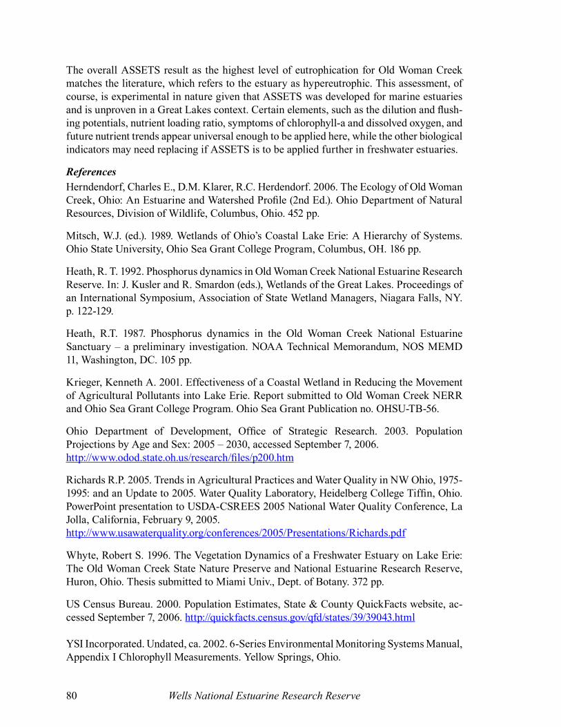
Wells National Estuarine Research Reserve80
The overall ASSETS result as the highest level of eutrophication for Old Woman Creek matches the literature, which refers to the estuary as hypereutrophic. This assessment, of course, is experimental in nature given that ASSETS was developed for marine estuaries and is unproven in a Great Lakes context. Certain elements, such as the dilution and flush-ing potentials, nutrient loading ratio, symptoms of chlorophyll-a and dissolved oxygen, and future nutrient trends appear universal enough to be applied here, while the other biological indicators may need replacing if ASSETS is to be applied further in freshwater estuaries.
ReferencesHerndendorf, Charles E., D.M. Klarer, R.C. Herdendorf. 2006. The Ecology of Old Woman Creek, Ohio: An Estuarine and Watershed Profile (2nd Ed.). Ohio Department of Natural Resources, Division of Wildlife, Columbus, Ohio. 452 pp.
Mitsch, W.J. (ed.). 1989. Wetlands of Ohio’s Coastal Lake Erie: A Hierarchy of Systems. Ohio State University, Ohio Sea Grant College Program, Columbus, OH. 186 pp.
Heath, R. T. 1992. Phosphorus dynamics in Old Woman Creek National Estuarine Research Reserve. In: J. Kusler and R. Smardon (eds.), Wetlands of the Great Lakes. Proceedings of an International Symposium, Association of State Wetland Managers, Niagara Falls, NY. p. 122-129.
Heath, R.T. 1987. Phosphorus dynamics in the Old Woman Creek National Estuarine Sanctuary – a preliminary investigation. NOAA Technical Memorandum, NOS MEMD 11, Washington, DC. 105 pp.
Krieger, Kenneth A. 2001. Effectiveness of a Coastal Wetland in Reducing the Movement of Agricultural Pollutants into Lake Erie. Report submitted to Old Woman Creek NERR and Ohio Sea Grant College Program. Ohio Sea Grant Publication no. OHSU-TB-56.
Ohio Department of Development, Office of Strategic Research. 2003. Population Projections by Age and Sex: 2005 – 2030, accessed September 7, 2006.http://www.odod.state.oh.us/research/files/p200.htm
Richards R.P. 2005. Trends in Agricultural Practices and Water Quality in NW Ohio, 1975-1995: and an Update to 2005. Water Quality Laboratory, Heidelberg College Tiffin, Ohio. PowerPoint presentation to USDA-CSREES 2005 National Water Quality Conference, La Jolla, California, February 9, 2005.http://www.usawaterquality.org/conferences/2005/Presentations/Richards.pdf
Whyte, Robert S. 1996. The Vegetation Dynamics of a Freshwater Estuary on Lake Erie: The Old Woman Creek State Nature Preserve and National Estuarine Research Reserve, Huron, Ohio. Thesis submitted to Miami Univ., Dept. of Botany. 372 pp.
US Census Bureau. 2000. Population Estimates, State & County QuickFacts website, ac-cessed September 7, 2006. http://quickfacts.census.gov/qfd/states/39/39043.html
YSI Incorporated. Undated, ca. 2002. 6-Series Environmental Monitoring Systems Manual, Appendix I Chlorophyll Measurements. Yellow Springs, Ohio.

Synthesis of SWMP and ASSETS for North Atlantic Region NERRs 81
Appendix II: Additional Land Use Index InformationThe MA-CZM Land Use Index (LUI) methodology calls for the analysis of the area ad-jacent to a wetland of interest. For some estuaries in this study (Great Bay, Waquoit Bay, Narragansett Bay), the GIS salinity zone coverage was considered to be essentially the same as the wetland system, because the adjacent marshes were very small relative to the overall size of the estuary. In the Webhannet and MBLR estuaries, however, the vegetated marsh comprises a large portion of the system beyond the channel. In the case of these estuaries, the marsh boundary was digitized separately, and land uses in the area surround-ing the entire system were determined. There appears to be no discernable pattern between either LUI and Overall Eutrophic Condition (OEC) or between LUI and ASSETS final grade, although this lack of correlation may be due to the very limited sample size of only five estuaries. Linear correlations result in an R2 of less than 0.1 (Figure 26).
This analysis brought to light an important difference between LUI and ASSETS. The land use method looks at impacts to the entire system, while ASSETS examines the eutrophic condition of estuarine waters. For the two estuaries in which the system boundaries were much larger than the channel boundaries, we conducted an additional analysis of land use immediately adjacent to the channel. In this case, there appears to be a correlation between both LUI and OEC (R2 = 0.69) and LUI and ASSETS (R2 = 0.84) (Figure 27).
ASSETS and Land Use Adjacent to System (Channel and Vegetated Marsh)
R2 = 1E-04
R2 = 0.0769
0
0.2
0.4
0.6
0.8
1
0 1 2 3 4 5 6
ASSETS or OEC Score
Lan
d U
se In
dex ASSETS vs. LUI
OEC vs. LUI
Linear (ASSETS vs.LUI)
Linear (OEC vs. LUI)
Table 26: ASSETS scores and Land Use Index according to original methodology, based on land surrounding the whole marsh system.
ASSETS and Land Use Adjacent to Channel
R2 = 0.69
R2 = 0.8425
0
0.2
0.4
0.6
0.8
1
0 1 2 3 4 5 6
ASSETS or OEC Score
Lan
d U
se In
dex ASSETS vs. LUI2
OEC vs. LUI2
Linear (ASSETS vs.LUI2)
Linear (OEC vs. LUI2)
Table 27: ASSET scores and Land Use Index, based on land surrounding the channel.

Wells National Estuarine Research Reserve82
Land Uses - 150 m Buffer
Natural Condition - 320 ac (46%)
Residential High - 266 ac (38%)
Urban - 60 ac (9%)
Maintained Open - 41 ac (6%)
Residential Low - 6 ac (1%)
Disturbed Open - 5 ac (<1%)
0 0.5 1Kilometers
Data Source: Maine Office of GIS; WNERRCoordinate System: NAD83, Zone 19, MetersMade by: F. Dillon - 6/11/06
WEBHANNET ESTUARYLand Use Assessment
Wells NERR - Wells, ME
M A I N E
Project Area
SWMP Stations
Figure 23: Land Use Index map for Webhannet Estuary. This map depicts the analysis of land use surrounding the entire channel-vegetated marsh system.
Webhannet Land Uses
Acres LUI Coeff. LUI Adj.
Natural Condition 319.5 0.95 303.6Residential High 266.0 0.25 66.5
Urban 60.4 0.23 13.9Maintained Open 40.5 0.83 33.6Residential Low 6.3 0.66 4.2Disturbed Open 5.3 0.86 4.6
698.2 426.4LUI GIS-based
score:0.61
Table 29: Webhannet Land Use Index using lands adjacent to the entire marsh system.

Synthesis of SWMP and ASSETS for North Atlantic Region NERRs 83
ASSETS-SWMP Data Synthesis ProjectWebhannet Estuary Land Use Analysis
150 m Buffer Land Uses *
Natural Condition - 831 ac. (86%)
Residential High - 88 ac. (9%)
Urban - 29 ac. (3%)
Maintained Open - 13 ac. (1%)
Residential Low - 4 ac. (<1%)
Disturbed Open - 2 ac. (<1%)
Data Source: Maine Office of GIS; WNERRCoordinate System: NAD83, UTM, Zone 19N, MetersMade by: F. Dillon on 11/29/06
0 1,000 2,000Feet
* MA-CZM LUI Score = 0.86
M A I N E
Wells NERR
Figure 24: Land Use Index map for Webhannet Estuary showing the analysis of land use adjacent to the channel only (the same GIS coverage that was used for the salinity zones).
Webhannet Land Uses
Acres LUI Coeff. LUI Adj.
Natural Condition 830.5 0.95 789.0Residential High 87.5 0.25 21.9
Urban 29.5 0.23 6.9Maintained Open 13.1 0.83 10.9Residential Low 4.0 0.66 2.7Disturbed Open 2.0 0.86 1.7
966.6 832.9LUI GIS-based
score:0.86
Table 30: Webhannet Land Use Index using lands adjacent to just the channel.
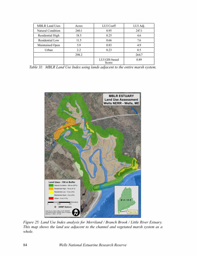
Wells National Estuarine Research Reserve84
MBLR ESTUARYLand Use Assessment
Wells NERR - Wells, ME
0 0.25 0.5Kilometers
Data Source: Maine Office of GIS; WNERRCoordinate System: NAD83, Zone 19, MetersMade by: F. Dillon - 6/11/06
Land Uses - 150 m BufferNatural Condition - 260 ac (87%)
Residential High - 19 ac (6 %)
Residential Low - 12 ac (4%)
Maintained Open - 6 ac (2%)
Urban - 2 ac (<1%)
SWMP Stations
M A I N E
Project Area
Figure 25: Land Use Index analysis for Merriland / Branch Brook / Little River Estuary. This map shows the land use adjacent to the channel and vegetated marsh system as a whole.
MBLR Land Uses Acres LUI Coeff LUI Adj.Natural Condition 260.1 0.95 247.1Residential High 18.5 0.25 4.6Residential Low 11.5 0.66 7.6
Maintained Open 5.9 0.83 4.9Urban 2.2 0.23 0.5
298.2 264.7LUI GIS-based
Score:0.89
Table 31: MBLR Land Use Index using lands adjacent to the entire marsh system.

Synthesis of SWMP and ASSETS for North Atlantic Region NERRs 85
ASSETS-SWMP Data Synthesis ProjectMBLR Estuary Land Use Analysis
* MA-CZM LUI Score = 0.91
M A I N E
Wells NERR
150 m Buffer Land Uses*
Natural Condition - 258 ac. (91%)
Residential High - 13 ac. (5%)
Residential Low - 5 ac. (2%)
Maintained Open - 4 ac. (1%)
Urban - 2 ac. (<1%)
Data Source: Maine Office of GIS; WNERRCoordinate System: NAD83, UTM, Zone 19N, MetersMade by: F. Dillon on 11/30/06
0 500 1,000Feet
Figure 26: Land Use Index analysis for Merriland / Branch Brook / Little River Estuary. This map shows the land use adjacent to the channel only.
MBLR Land Uses Acres LUI Coeff LUI Adj.Natural Condition 258.2 0.95 245.3Residential High 13.3 0.25 3.3Residential Low 4.7 0.66 3.1
Maintained Open 4.3 0.83 3.6Urban 2.0 0.23 0.5
282.5 255.7LUI GIS-based
Score:0.91
Table 32: MBLR Land Use Index using lands adjacent to just the channel.

Wells National Estuarine Research Reserve86
ASSETS-SWMP Data Synthesis ProjectGreat Bay Land Use Analysis
150 m Buffer Land Uses *
Natural Condition - 5,465 ac (56%)
Residential Low - 1,521 ac (16%)
Agricultural - 670 ac (7%)
Urban - 636 ac (6%)
Maintained Open - 532 ac (5%)
Disturbed Open - 454 ac (5%)
Residential High - 395 ac (4%)
Residential Medium - 127 ac (1%)
GBNERR SWMP Stations
0 1 2 3 4 5Miles
Data Sources: NH Granit; ME Office of GISCoordinate Systems: NAD83, UTM, Zone 19N, metersCreated: 11/21/06 by F. Dillon
M A I N E
N. H.
Great BayNERR
* MA CZM LUIScore = 0.81
Figure 29: Land Use Index map for Great Bay Estuary.
Great Bay Land Uses Acres LUI Coeff LUI AdjNatural Condition 5464 0.95 5191Residential Low 1521 0.66 1004
Agricultural 670 0.83 556Urban 636 0.23 146
Maintained Open 532 0.83 441Disturbed Open 454 0.86 390Residential High 395 0.25 99
Residential Medium 127 0.45 579799 7885
LUI GIS-based Score:
0.80
Table 34: Great Bay Land Use Index using lands adjacent to the entire marsh system.
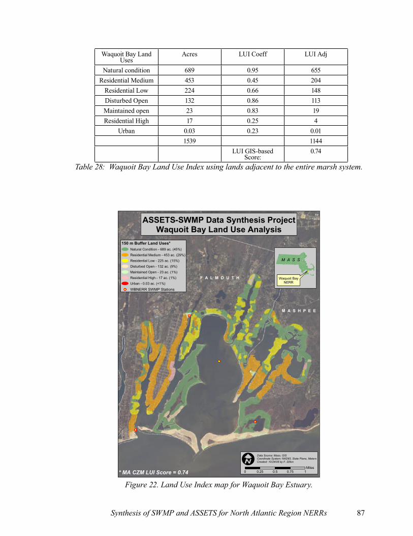
Synthesis of SWMP and ASSETS for North Atlantic Region NERRs 87
ASSETS-SWMP Data Synthesis ProjectWaquoit Bay Land Use Analysis
150 m Buffer Land Uses*Natural Condition - 689 ac. (45%)
Residential Medium - 453 ac. (29%)
Residential Low - 225 ac. (15%)
Disturbed Open - 132 ac. (9%)
Maintained Open - 23 ac. (1%)
Residential High - 17 ac. (1%)
Urban - 0.03 ac. (<1%)
WBNERR SWMP Stations
M A S S
Waquoit BayNERR
0 0.25 0.5 0.75 1Miles
Data Source: Mass. GISCoordinate System: NAD83, State Plane, MetersCreated: 10/24/06 by F. Dillon
* MA CZM LUI Score = 0.74
F A L M O U T H
M A S H P E E
Figure 22. Land Use Index map for Waquoit Bay Estuary.
Waquoit Bay Land Uses
Acres LUI Coeff LUI Adj
Natural condition 689 0.95 655Residential Medium 453 0.45 204
Residential Low 224 0.66 148Disturbed Open 132 0.86 113Maintained open 23 0.83 19Residential High 17 0.25 4
Urban 0.03 0.23 0.011539 1144
LUI GIS-based Score:
0.74
Table 28: Waquoit Bay Land Use Index using lands adjacent to the entire marsh system.
Wells National Estuarine Research Reserve88
Figure 27: Land Use Index map for Narragansett Bay Estuary.
ASSETS-SWMP Data Synthesis ProjectNarragansett Bay Land Use Analysis
M A S S A C H U S E T T S
R H O D E I S L A N D
NarragansettBay
M E
N H
M A
R IC T
Data Sources: Rhode Island GIS; Mass GISCoordinate System: NAD83, State Plane RI, FeetCreated by: F. Dillon - 9/11/06
0 2 4 6Miles
NBNERR SWMP Stations
150m Landuse Buffer
Narragansett Bay Land Uses
Acres LUI Coeff LUI Adj
Natural 6051 0.95 5748Residential High 2909 0.25 727
Urban 2770 0.23 637Residential Medium 2328 0.45 1048
Disturbed Open 1670 0.86 1436Maintained Open 1115 0.83 926Residential Low 743 0.66 490
Agriculture 742 0.83 61618327 11628
LUI GIS-based Score:
0.63
Table 33: Narragansett Bay Land Use Index using lands adjacent to the entire marsh system.
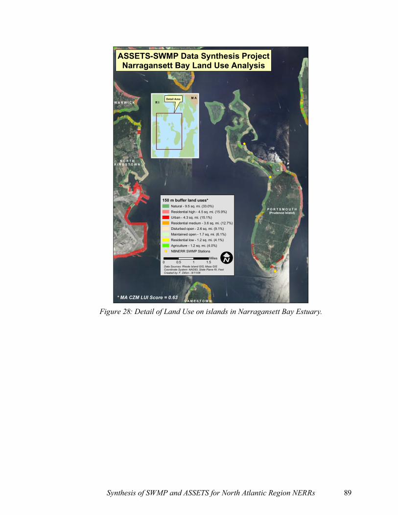
Synthesis of SWMP and ASSETS for North Atlantic Region NERRs 89
ASSETS-SWMP Data Synthesis ProjectNarragansett Bay Land Use Analysis
Detail Area M AR I
Data Sources: Rhode Island GIS; Mass GISCoordinate System: NAD83, State Plane RI, FeetCreated by: F. Dillon - 9/11/06
0 0.5 1 1.5Miles
150 m buffer land uses*Natural - 9.5 sq. mi. (33.0%)
Residential high - 4.5 sq. mi. (15.9%)
Urban - 4.3 sq. mi. (15.1%)
Residential medium - 3.6 sq. mi. (12.7%)
Disturbed open - 2.6 sq. mi. (9.1%)
Maintained open - 1.7 sq. mi. (6.1%)
Residential low - 1.2 sq. mi. (4.1%)
Agriculture - 1.2 sq. mi. (4.0%)
NBNERR SWMP Stations
N O R T HK I N G S T O W N
W A R W I C K
P O R T S M O U T H(Prudence Island)
* MA CZM LUI Score = 0.63J A M E S T O W N
Figure 28: Detail of Land Use on islands in Narragansett Bay Estuary.

Wells National Estuarine Research Reserve90
Appendix III: Maps of ASSETS Component Results
Figure 30: Map of flushing Potential. Figure 31: Map of Dilution Potential.
Figure 32: Map of Susceptibility.
Figure 33: Map of Influencing Factors.
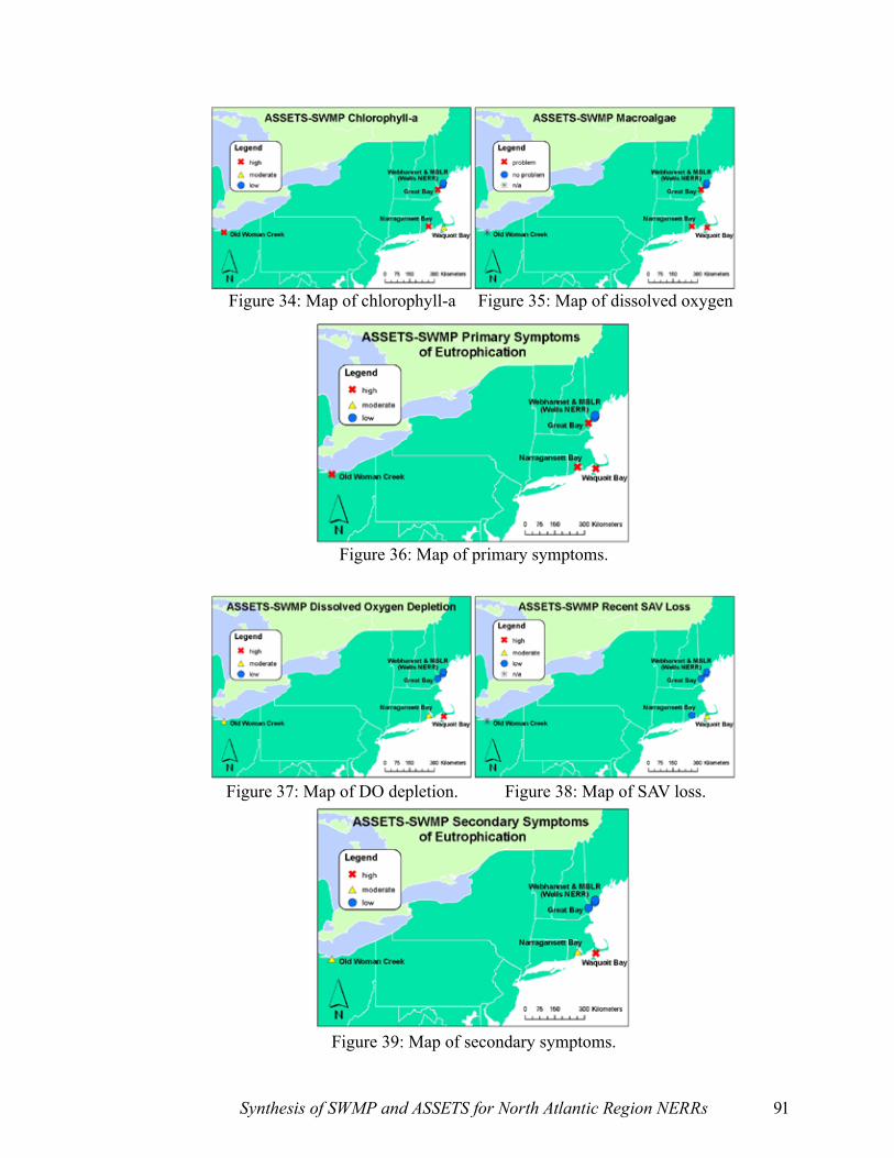
Synthesis of SWMP and ASSETS for North Atlantic Region NERRs 91
Figure 34: Map of chlorophyll-a Figure 35: Map of dissolved oxygen
Figure 37: Map of DO depletion. Figure 38: Map of SAV loss.
Figure 39: Map of secondary symptoms.
Figure 36: Map of primary symptoms.
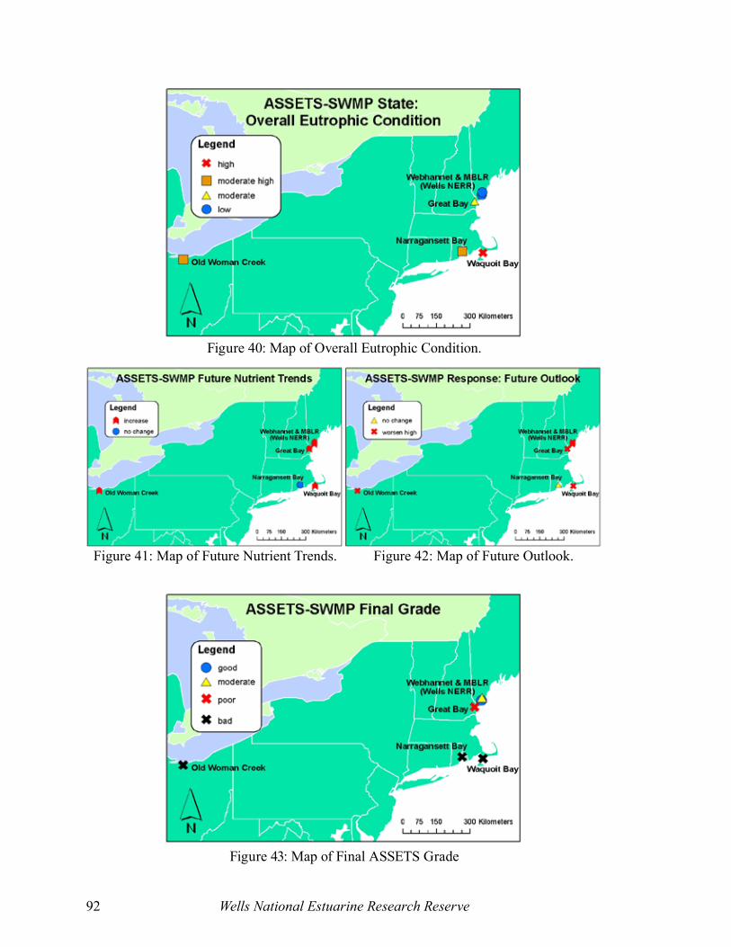
Wells National Estuarine Research Reserve92
Figure 40: Map of Overall Eutrophic Condition.
Figure 43: Map of Final ASSETS Grade
Figure 41: Map of Future Nutrient Trends. Figure 42: Map of Future Outlook.


![2019 STORMWATER MANAGEMENT PROGRAM PLAN UPDATEci.brier.wa.us › pdf › Brier SWMP 2019 [146728].pdf · the City’s Stormwater Management Program (SWMP). The City’s SWMP is intended](https://static.fdocuments.in/doc/165x107/5f0d8e2f7e708231d43af09f/2019-stormwater-management-program-plan-a-pdf-a-brier-swmp-2019-146728pdf.jpg)