Synthesis of Protocols and Discrete Controllerscgi.csc.liv.ac.uk/~sven/IdressHusien.pdf · I would...
123
Synthesis of Protocols and Discrete Controllers Thesis submitted in accordance with the requirements of the University of Liverpool for the degree of Doctor in Philosophy by Idress Mohammed Husien November 2017
Transcript of Synthesis of Protocols and Discrete Controllerscgi.csc.liv.ac.uk/~sven/IdressHusien.pdf · I would...

Synthesis of Protocols and Discrete Controllers
Thesis submitted in accordance with the requirements ofthe University of Liverpool for the degree of Doctor in Philosophy by
Idress Mohammed Husien
November 2017


Dedication
To My family
iii

Contents
notation v
Notations xiii
Preface xv
Abstract xvii
Acknowledgements xix
1 Introduction 11.1 Overview . . . . . . . . . . . . . . . . . . . . . . . . . . . . . . . . . . . . 11.2 Motivation . . . . . . . . . . . . . . . . . . . . . . . . . . . . . . . . . . . . 21.3 Research Question . . . . . . . . . . . . . . . . . . . . . . . . . . . . . . . 31.4 Research Methodology . . . . . . . . . . . . . . . . . . . . . . . . . . . . . 31.5 Research Contribution . . . . . . . . . . . . . . . . . . . . . . . . . . . . . 5
1.5.1 Program Synthesis . . . . . . . . . . . . . . . . . . . . . . . . . . . 51.5.2 Controller synthesis . . . . . . . . . . . . . . . . . . . . . . . . . . 5
1.6 The Organization of Thesis . . . . . . . . . . . . . . . . . . . . . . . . . . 61.7 Publication . . . . . . . . . . . . . . . . . . . . . . . . . . . . . . . . . . . 71.8 Summery . . . . . . . . . . . . . . . . . . . . . . . . . . . . . . . . . . . . 9
2 Background 112.1 Introduction . . . . . . . . . . . . . . . . . . . . . . . . . . . . . . . . . . . 112.2 Search Techniques . . . . . . . . . . . . . . . . . . . . . . . . . . . . . . . 11
2.2.1 Simulated Annealing . . . . . . . . . . . . . . . . . . . . . . . . . 122.2.2 Genetic Programming . . . . . . . . . . . . . . . . . . . . . . . . . 132.2.3 Initialization . . . . . . . . . . . . . . . . . . . . . . . . . . . . . . 15
2.3 Genetic Operators . . . . . . . . . . . . . . . . . . . . . . . . . . . . . . . 152.3.1 Mutation . . . . . . . . . . . . . . . . . . . . . . . . . . . . . . . . 152.3.2 Crossover . . . . . . . . . . . . . . . . . . . . . . . . . . . . . . . . 15
2.4 Hybrid Genetic Programming . . . . . . . . . . . . . . . . . . . . . . . . . 162.5 Model checking . . . . . . . . . . . . . . . . . . . . . . . . . . . . . . . . . 17
2.5.1 Computation Tree Logic (CTL) . . . . . . . . . . . . . . . . . . . . 17
v
3 Program Synthesis 213.1 Abstract . . . . . . . . . . . . . . . . . . . . . . . . . . . . . . . . . . . . . 213.2 Introduction . . . . . . . . . . . . . . . . . . . . . . . . . . . . . . . . . . . 223.3 The Approach in a Nutshell . . . . . . . . . . . . . . . . . . . . . . . . . . 243.4 Model Checking as a Fitness Function . . . . . . . . . . . . . . . . . . . . 263.5 Programs as Trees . . . . . . . . . . . . . . . . . . . . . . . . . . . . . . . 273.6 Case Studies . . . . . . . . . . . . . . . . . . . . . . . . . . . . . . . . . . . 31
3.6.1 Mutual Exclusion . . . . . . . . . . . . . . . . . . . . . . . . . . . . 313.6.2 Leader Election . . . . . . . . . . . . . . . . . . . . . . . . . . . . . 32
3.7 Synthesis Approach . . . . . . . . . . . . . . . . . . . . . . . . . . . . . . . 333.7.1 Parameters Setting . . . . . . . . . . . . . . . . . . . . . . . . . . . 333.7.2 Temperature Range . . . . . . . . . . . . . . . . . . . . . . . . . . 343.7.3 Crossover Ratio . . . . . . . . . . . . . . . . . . . . . . . . . . . . . 363.7.4 Initial Population Size Cost . . . . . . . . . . . . . . . . . . . . . . 36
3.8 Evaluation . . . . . . . . . . . . . . . . . . . . . . . . . . . . . . . . . . . . 373.9 Discussion . . . . . . . . . . . . . . . . . . . . . . . . . . . . . . . . . . . . 42
4 Discrete Controller Synthesis 454.1 Abstract . . . . . . . . . . . . . . . . . . . . . . . . . . . . . . . . . . . . . 454.2 Introduction . . . . . . . . . . . . . . . . . . . . . . . . . . . . . . . . . . . 45
4.2.1 General Search Techniques . . . . . . . . . . . . . . . . . . . . . . . 464.2.2 Contributions . . . . . . . . . . . . . . . . . . . . . . . . . . . . . . 47
4.3 Symbolic Model Checking & Controller Synthesis . . . . . . . . . . . . . . 474.3.1 Predicates . . . . . . . . . . . . . . . . . . . . . . . . . . . . . . . . 474.3.2 Symbolic Transition Systems . . . . . . . . . . . . . . . . . . . . . 48
Semantics . . . . . . . . . . . . . . . . . . . . . . . . . . . . 494.3.3 Model Checking STSs . . . . . . . . . . . . . . . . . . . . . . . . . 50
CTL w.r.t. STSs . . . . . . . . . . . . . . . . . . . . . . . . 504.4 Symbolic Discrete Controller Synthesis . . . . . . . . . . . . . . . . . . . . 51
4.4.1 Principles of Traditional DCS Algorithms . . . . . . . . . . . . . . 524.4.2 Symbolic DCS . . . . . . . . . . . . . . . . . . . . . . . . . . . . . 524.4.3 Controlled Execution of STSs . . . . . . . . . . . . . . . . . . . . . 534.4.4 Obtaining a Deterministic Controlled STS . . . . . . . . . . . . . . 53
4.5 Contribution w.r.t. Symbolic DCS . . . . . . . . . . . . . . . . . . . . . . 544.5.1 General Search Techniques . . . . . . . . . . . . . . . . . . . . . . . 554.5.2 Random Generation of Candidates . . . . . . . . . . . . . . . . . . 56
4.6 Principles of our DCS Algorithms . . . . . . . . . . . . . . . . . . . . . . . 574.6.1 Representing Deterministic Strategies . . . . . . . . . . . . . . . . 574.6.2 Performing Mutations and Crossovers . . . . . . . . . . . . . . . . 584.6.3 Model checking as a Fitness Function . . . . . . . . . . . . . . . . 604.6.4 Variants for Improved Search Techniques . . . . . . . . . . . . . . . 61
4.7 Experimental Feasibility Assessment . . . . . . . . . . . . . . . . . . . . . 624.7.1 Problem Instances . . . . . . . . . . . . . . . . . . . . . . . . . . . 62
Partial Objectives . . . . . . . . . . . . . . . . . . . . . . . . 634.7.2 Experimental Setup . . . . . . . . . . . . . . . . . . . . . . . . . . 644.7.3 Experimental Results . . . . . . . . . . . . . . . . . . . . . . . . . 64
4.8 Parameters Setting . . . . . . . . . . . . . . . . . . . . . . . . . . . . . . . 67
vi

4.8.1 Crossover Ratio . . . . . . . . . . . . . . . . . . . . . . . . . . . . . 674.8.2 Temperature . . . . . . . . . . . . . . . . . . . . . . . . . . . . . . 694.8.3 Initial Population vs Cost . . . . . . . . . . . . . . . . . . . . . . . 714.8.4 Discussion . . . . . . . . . . . . . . . . . . . . . . . . . . . . . . . . 71
5 Complexity 775.1 Introduction . . . . . . . . . . . . . . . . . . . . . . . . . . . . . . . . . . . 775.2 Complexity Analysis . . . . . . . . . . . . . . . . . . . . . . . . . . . . . . 78
5.2.1 Program Synthesis . . . . . . . . . . . . . . . . . . . . . . . . . . . 785.2.2 Discrete Controller Synthesis . . . . . . . . . . . . . . . . . . . . . 79
6 Implementation 836.1 Abstract . . . . . . . . . . . . . . . . . . . . . . . . . . . . . . . . . . . . . 836.2 Introduction . . . . . . . . . . . . . . . . . . . . . . . . . . . . . . . . . . . 836.3 Overview of PranCS . . . . . . . . . . . . . . . . . . . . . . . . . . . . . . 85
6.3.1 Representing Candidates . . . . . . . . . . . . . . . . . . . . . . . . 856.3.2 Structure of PranCS . . . . . . . . . . . . . . . . . . . . . . . . . . 866.3.3 Selecting and Tuning Search Techniques . . . . . . . . . . . . . . . 876.3.4 Parameters for Simulated Annealing . . . . . . . . . . . . . . . . . 886.3.5 Parameters for Genetic Programming . . . . . . . . . . . . . . . . 89
6.4 Exploration of the Parameter Space . . . . . . . . . . . . . . . . . . . . . 896.4.1 Exploring Population Size & Crossover Ratio . . . . . . . . . . . . 896.4.2 Exploring Cooling Schedules . . . . . . . . . . . . . . . . . . . . . . 90
6.5 Conclusion . . . . . . . . . . . . . . . . . . . . . . . . . . . . . . . . . . . . 90
7 Conclusion 937.1 Summery . . . . . . . . . . . . . . . . . . . . . . . . . . . . . . . . . . . . 937.2 Main Findings and Contributions . . . . . . . . . . . . . . . . . . . . . . . 94
7.2.1 Program synthesis . . . . . . . . . . . . . . . . . . . . . . . . . . . 967.2.2 Controller synthesis . . . . . . . . . . . . . . . . . . . . . . . . . . 96
Bibliography 99
vii


Illustrations
List of Figures
1.1 Work Flow Chart . . . . . . . . . . . . . . . . . . . . . . . . . . . . . . . . . 4
2.1 Simulated Annealing Flow Chart . . . . . . . . . . . . . . . . . . . . . . . . . 122.2 Genetic Programming Flow Chart . . . . . . . . . . . . . . . . . . . . . . . . 142.3 GP Candidate Tree . . . . . . . . . . . . . . . . . . . . . . . . . . . . . . . . 152.4 Candidate tree (left) with one node mutations (right) . . . . . . . . . . . . . 162.5 Program tree (left) with sub-tree mutations (right) . . . . . . . . . . . . . . . 162.6 Crossover:two parents(above)and two offspring (below) . . . . . . . . . . . . 172.7 Model Checking . . . . . . . . . . . . . . . . . . . . . . . . . . . . . . . . . . 18
3.1 Synthes Tool . . . . . . . . . . . . . . . . . . . . . . . . . . . . . . . . . . . . 253.2 Program tree (left) with one node mutations (right) . . . . . . . . . . . . . . 273.3 Program tree (left) with sub-tree mutations (right) . . . . . . . . . . . . . . . 273.4 Crossover:two parents(above)and two offspring (below) . . . . . . . . . . . . 283.5 Translation example – source(left) and target (right) . . . . . . . . . . . . . . 293.6 Synthesized Programs . . . . . . . . . . . . . . . . . . . . . . . . . . . . . . . 323.7 Graphical User Interface . . . . . . . . . . . . . . . . . . . . . . . . . . . . . . 343.8 Initial Population Size vs Cost for SW Synthesis . . . . . . . . . . . . . . . . 393.9 Average time required for synthesising a correct program . . . . . . . . . . . 413.10 Average running time of an individual execution . . . . . . . . . . . . . . . . 413.11 success rate of individual executions . . . . . . . . . . . . . . . . . . . . . . . 42
4.1 STS STask (Example 4.1) as a guarded automaton. . . . . . . . . . . . . . . . 504.2 Candidate predicate (left) with one node mutation (right) . . . . . . . . . . . 594.3 Candidate predicate (left) with sub-tree mutation (right) . . . . . . . . . . . 594.4 Crossover: two parents (above) and two offspring (below) . . . . . . . . . . . 604.5 Overall time required for synthesising a correct candidate . . . . . . . . . . . 654.6 Average running time of an individual execution . . . . . . . . . . . . . . . . 654.7 Success rate of individual executions . . . . . . . . . . . . . . . . . . . . . . . 664.8 Temperature Range for Controller Synthesis . . . . . . . . . . . . . . . . . . 744.9 Initial Population Size vs Cost for Discrete Controller synthesis . . . . . . . . 75
6.1 PranCS Structure . . . . . . . . . . . . . . . . . . . . . . . . . . . . . . . . . 856.2 Graphical User Interface. PranCS allows the user to fine-tune each search
technique by means of dedicated parameters. . . . . . . . . . . . . . . . . . 88
ix


List of Tables
3.1 Comparison for search temperature for Leader Election . . . . . . . . . . . . 353.2 Comparison for search temperature for Mutual Exclusion . . . . . . . . . . . 363.3 Crossover ratio for GP (Program Synthesis) . . . . . . . . . . . . . . . . . . . 373.4 Crossover ratio for Hybrid (Program Synthesis) . . . . . . . . . . . . . . . . . 383.5 Population size vs cost for Program synthesis (2-shared bit mutual exclusion) 393.6 Population size vs cost for Program synthesis (2-shared bit mutual exclusion) 403.7 Search Techniques Comparison . . . . . . . . . . . . . . . . . . . . . . . . . . 43
4.1 Search Techniques Comparison . . . . . . . . . . . . . . . . . . . . . . . . . . 674.2 Crossover ratio for GP (Discrete Controller Synthesis) . . . . . . . . . . . . . 684.3 Crossover ratio for Hybrid (Discrete Controller Synthesis) . . . . . . . . . . . 694.4 Population size vs cost for GP (Discrete Controller synthesis 2-Tasks) . . . . 704.5 Population size vs cost for Hybrid (Discrete Controller synthesis 2-Tasks) . . 714.6 Comparison for search temperature for Discrete Controller synthesis . . . . . 724.7 Comparison for search temperature for Discrete Controller . . . . . . . . . . 73
6.1 Synthesis times with the best parameters observed for Simulated Annealingapplied to our DCS benchmarks . . . . . . . . . . . . . . . . . . . . . . . . . 90
6.2 On the left: Safety-first GP with crossover for DCS (2-Tasks only), withVarious Population Sizes (|P |). . . . . . . . . . . . . . . . . . . . . . . . . . 90
xi

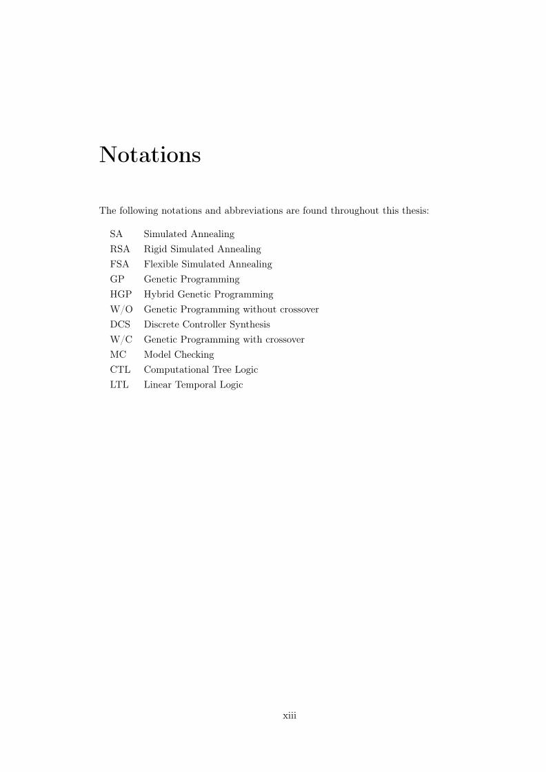
Notations
The following notations and abbreviations are found throughout this thesis:
SA Simulated AnnealingRSA Rigid Simulated AnnealingFSA Flexible Simulated AnnealingGP Genetic ProgrammingHGP Hybrid Genetic ProgrammingW/O Genetic Programming without crossoverDCS Discrete Controller SynthesisW/C Genetic Programming with crossoverMC Model CheckingCTL Computational Tree LogicLTL Linear Temporal Logic
xiii


Preface
I declare that this thesis is composed by myself and that the work contained herein is myown, except where explicitly stated otherwise, and that this work was undertaken by meduring my period of study at the University of Liverpool, United Kingdom. This thesishas not been submitted for any other degree or qualification except as specified here.
xv

Abstract
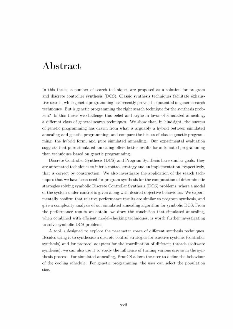
In this thesis, a number of search techniques are proposed as a solution for programand discrete controller synthesis (DCS). Classic synthesis techniques facilitate exhaus-tive search, while genetic programming has recently proven the potential of generic searchtechniques. But is genetic programming the right search technique for the synthesis prob-lem? In this thesis we challenge this belief and argue in favor of simulated annealing,a different class of general search techniques. We show that, in hindsight, the successof genetic programming has drawn from what is arguably a hybrid between simulatedannealing and genetic programming, and compare the fitness of classic genetic program-ming, the hybrid form, and pure simulated annealing. Our experimental evaluationsuggests that pure simulated annealing offers better results for automated programmingthan techniques based on genetic programming.
Discrete Controller Synthesis (DCS) and Program Synthesis have similar goals: theyare automated techniques to infer a control strategy and an implementation, respectively,that is correct by construction. We also investigate the application of the search tech-niques that we have been used for program synthesis for the computation of deterministicstrategies solving symbolic Discrete Controller Synthesis (DCS) problems, where a modelof the system under control is given along with desired objective behaviours. We experi-mentally confirm that relative performance results are similar to program synthesis, andgive a complexity analysis of our simulated annealing algorithm for symbolic DCS. Fromthe performance results we obtain, we draw the conclusion that simulated annealing,when combined with efficient model-checking techniques, is worth further investigatingto solve symbolic DCS problems.
A tool is designed to explore the parameter space of different synthesis techniques.Besides using it to synthesise a discrete control strategies for reactive systems (controllersynthesis) and for protocol adapters for the coordination of different threads (softwaresynthesis), we can also use it to study the influence of turning various screws in the syn-thesis process. For simulated annealing, PranCS allows the user to define the behaviourof the cooling schedule. For genetic programming, the user can select the populationsize.
xvii


Acknowledgements
I would like to express my deepest gratitude to my first supervisor, Sven Schewe, speciallyfor his support, constant patience and encouragement throughout my years of study. Hehas been very supportive in many different ways and has constantly encouraged meduring all these years. His immense knowledge has always helped me to learn a lot fromhim. His friendly behaviour and positive attitude are exemplary and I regard it as myhonour to have done my Ph.D. under his excellent supervision.
I would like to thank Alexei Lisitsa, and David Jackson, for being my academicadvisors, Dominik Wojtczak, for being my second supervisor and Special thanks also goto Nicolas Berthier for his support. I thank them for all their advice, useful ideas andsupport.
I would like to extend my deepest gratitude to the Ministry of higher Education inIraq especially the University of Kirkuk and Iraqi Cultural Attaché in London for theirfinancial support and for providing me with the opportunity to conduct my Ph.D. study.
I would like to thank the Department of Computer Science at the University of Liv-erpool has been an excellent place to conduct research; all staff members and colleagueshave been helpful whenever necessary. Finally, I thank my family, for all their support,trust, encouragement and prayers.
xix


Chapter 1
Introduction
1.1 Overview
The development of correct code can be quite challenging, especially for concurrentsystems. Classical software engineering methods, where the validation is based on testing,do not seem to provide the right way to approach this type of involved problems, as bugseasily elude predefined tests. Guaranteeing correctness for such programs is also nottrivial. Manual proof methods for verifying the correctness of the code against a givenformal specification were suggested in the late 60s.
The next step for achieving more reliable software has been to offer an automaticverification procedure through model checking [CGP99, BCM+90, AHM+98]. The holygrail of such techniques would be automatic synthesis: the automated construction ofprograms that are correct by construction.
Such synthesis techniques have long been held to be impossible due to complexity(which ranges between EXPTIME for CTL synthesis [CE82] and undecidable [PR90,FS05, SF06] for distributed systems. This line of thought has come under attack onmany fronts.
On the theoretical side, bounded [FS13] and succinct [FPS15] synthesis techniqueshave leveled the playing field between verification and synthesis by shifting the focusfrom the input complexity to the cost measured in the minimal explicit and symbolicsolution, respectively. One could argue that this is the theoretical foundation of successfulapproaches, including implementations of bounded synthesis [FJR09, Ehl11] and methodsbased on genetic algorithms [Joh07, KP08, KP09a].
In this work we suggest to use simulated annealing for program synthesis and compareit to similar approaches based on genetic algorithms. We use formal verification technique(model checking) as a way for assessing fitness in an inductive automatic programmingsystem.
We have implemented a synthesising tool, which uses (multiple calls to) the modelchecker NuSMV to determine the fitness for a candidate program. The candidate pro-grams exist in two forms. The main form is a simple imperative language. This formis subject to mutation, but it is translated to a secondary form, the modeling language
1
Chapter 1. Introduction 2
of NuSMV, for evaluating the fitness. We have implemented different selection andupdate mechanism to compare the performance of simulated annealing with genetic pro-gramming. Genetic programming represented in this work with and without applyingcrossover. A hybrid genetic programming method also applied in this work beside sim-ulated annealing.
The remainder of this introductory chapter is organised as follows. Section 1.2presents the motivation for the work presented in this thesis. Section 1.3 describes themain research question and the associated research issues to be addressed by the thesis.The adopted research methodology is presented in Section 1.4. Section 1.5 describes thecontributions of the work presented. The organisation of the remainder of this thesis ispresented in Section 1.6. Section 1.7 lists the publications resulting from the researchpresented in this thesis. Finally this chapter is concluded in Section 1.8 with a briefsummary.
1.2 Motivation
The main aim of the work presented in this thesis is to investigate and evaluate effectivealgorithms that will be used for code generation especially for concurrent programmingand for discrete controller synthesis. The motivation for this work is that the synthesisof programs and discrete controllers is desirable because it provides the following :
1. It can be used for generating correct code, which can be quite challenging especiallyfor concurrent systems, that cannot be obtained efficiently by classical softwareengineering methods.
2. It allows to correct the errors in faulty code by verifying a desired specificationsusing model checking, which takes a model and properties as input and check ifthe model satisfies the objectives or not, and lets the implementation evolve intocorrect code.
3. It can also be used for the computation of deterministic strategies solving symbolicDiscrete Controller Synthesis (DCS) problems, where a model of the system tocontrol is given along with desired objective behaviours.
The challenge in automatic programming is synthesizing programs automatically fromtheir set of requirements. Search techniques in which the fitness of each program is usuallycalculated by running the program on some test cases, and evaluating its performance.Orthogonally, model checking can be used to analyze a given program, verifying that itsatisfies its specification, or providing a counterexample of that fact.
Discrete Controller Synthesis (DCS) and Program Synthesis have similar goals inthat they are constructive methods for behaviour control. Discrete controller synthesistypically operates on the model of a plant, and seeks the automated construction ofa strategy so that the plant controlled accordingly satisfies a specific set of specifica-tions. Likewise, program synthesis operates by using some predefined rules, such as the

Chapter 1. Introduction 3
grammar and semantics of the target programming language, and seeks the automatedconstruction of a program whose execution satisfies a specific set of specifications.
As noted above the search techniques can be used together the model checking asa way to synthesis both programs and discrete controllers. The motivation of the workdescribed in this thesis can thus broadly be identified as the desire to develop a synthesistechnique that has low cost and can be used for both programs and discrete controllers.
1.3 Research Question
From the research motivation presented in Section 1.2, the key objective of the workpresented in this thesis is to research and investigate effective and efficient techniquefor program and controller synthesis. This objective can be formulated as a researchquestion as follows:
What are the most appropriate search technique that can be used with model checking(as a fitness function) for program so as control synthesis
In order to answer this research question the resolution of a number of sub-questionis required. These questions can be summarized as follows:
• General Search Technique: What is the best search technique that can be usedfor program synthesis? Is genetic programming, simulated annealing, or a hybridof them better? Can we implement them in another way as hybrid methods?
• Search Techniques Parameters: What are the efficient parameters that canbe used for genetic programming and simulated annealing? Is the application ofcrossover effective? How does initial population size affect the cost beside thesuccess rate? How does the initial temperature and cooling schedule affect theresults of simulated annealing? Are there ’best’ parameters for our techniques?
• Controller Synthesis: Can we use the same techniques in controller synthesis?Are the results similar to those of program synthesis? What about the parametersdo they have the same effect?
• Synthesis Tool: What is the scope of a synthesis tool based on generic searchtechnique?
1.4 Research Methodology
As described in the previous sections, the adopted research methodology of the workdescribed in this thesis is to investigate and evaluate a series of techniques used forprogram and controller synthesis. For this purpose, simulated annealing is used forprogram synthesis and compared it to similar approaches based on genetic programming.
We use a formal verification technique, model checking, as a way of assessing its fitnessin an inductive automatic programming system. We have implemented a synthesis tool,

Chapter 1. Introduction 4
which uses multiple calls to the model checker NuSMV [CCG+02] to determine the fitnessfor a candidate. The candidates exist in two forms.
1. The main form is a simple imperative language. This form is subject to mutation,in which the program represented as a binary tree. The leaf nodes in the programtree is the variables or constant. The program tree translated to
2. a secondary form, the modeling language of NuSMV, for evaluating its fitness.
Figure 1.1: Work Flow Chart
While there has been further research on how to measure partial satisfaction [HO13],we have adopted an approach that retains with the previous attempts:
1. The best choice for us is to keep to the choices made for promoting genetic pro-gramming [KP08, KP09a, KP09b], as this is the only choice that is completely freeof suspicion of being selected for being more suitable for simulated annealing thanfor genetic programming.
2. A second motivation for this selection is that it results in very simple specificationsand, therefore, in fast evaluations of the fitness.
Noting that synthesis entails on average hundreds of thousands to millions of calls toa model checker, only simple evaluations can be considered. We have implemented sixdifferent combinations of selection and update mechanism to test our hypothesis:
1. Simulated annealing with two different fitness measure.
2. Genetic programming both without crossover (as discussed in [KP08, KP09a, KP09b])and with crossover.
Chapter 1. Introduction 5
3. Hybrid genetic programming both without crossover (as discussed in [KP08, KP09a,KP09b]) and with crossover.
At the beginning all the parameters initialized, then the initial population generatedby the generation part of the our software, initially the candidates represented as a binarytrees. The candidates trees used as input for the translator, which convert them into aNuSMV models to evaluate those candidates. The model checker use as fitness functionfor the search techniques.
1.5 Research Contribution
1.5.1 Program Synthesis
In this part of our work we implement the following approaches:
1. We use simulated annealing for program synthesis and compare it to similar ap-proaches based on genetic programming.
2. We use a formal verification technique, model checking, as a way of assessing itsfitness in an inductive automatic programming system. For this purpose we give ascore for a candidate depending on the satisfied specifications.
3. We have implemented a synthesis tool, which uses multiple calls to the modelchecker NuSMV [CCG+02] to determine the fitness for a candidate program. Thetool enables the user to input the requirements (as temporal logic specifications)ofthe programs (protocols) that (s)he wants to generate, and the input variables forthe algorithms.
4. We have implemented six different combinations of selection and update mecha-nism to test our hypothesis: besides simulated annealing, we have used geneticprogramming both without crossover (as discussed in [KP08, KP09a, KP09b]) andwith crossover and hybrid genetic programming both without crossover (as dis-cussed in [KP08, KP09a, KP09b]) and with crossover. Simulated annealing alsoimplemented in two forms depending on the sharing of specifications. If the safetyspecification considered first then we refer to simulated annealing as flexible oth-erwise it will be knowns as rigid simulated annealing.
The tests we have run confirmed that simulated annealing performs significantlybetter than genetic programming. As a side result, we found that the assumption of Katzand Peled [KP08, KP09a, KP09b] that crossover does not accelerate genetic programmingdid not prove to be entirely correct, but the advantages we observed were minor.
1.5.2 Controller synthesis
1. We first define a symbolic model and an associated class of DCS problems, forwhich deterministic strategies are sought.

Chapter 1. Introduction 6
2. Next, we adapt the aforementioned search techniques to obtain algorithmic solu-tions that avoid computing the unsafe portion of the state-space.
3. Then, we confirm the hypotheses that (i) general search techniques are as applicableto solve our DCS problem as they are for synthesising programs; and
(ii) one obtains similar relative performance results for our DCS problem. Exper-imental results [HS16] for program synthesis, essentially that simulated annealingperforms better than genetic programming.
4. To assess these hypotheses, we adapt the six different combinations of candidateselection and update mechanisms of our previous work [HS16], and execute themon a scalable example DCS problem.
5. We perform an experimental feasibility assessment.
From the performance results we obtain, we draw the conclusion that, even thoughfor technical reasons our current experimental results do not compare favourably withexisting symbolic DCS tools, simulated annealing, when combined with efficient model-checking techniques, is worth further investigating to solve symbolic DCS problems.
1.6 The Organization of Thesis
The rest of the thesis delves in detail into the work behind each of the contributions, andis organized as follows:
• In Chapter 2 We present a literature review of related research and some back-ground material to the work on the search techniques explained in this thesis.
• Chapter 3 presents the adaptation of the general search techniques to solve theprogram synthesis problem and an extension of the quest for the best general searchtechnique by studying the effect of the parameter settings for the individual searchtechniques: the influence of the selected temperature for simulated annealing andthe crossover ratio for genetic programming.
• Chapter 4 summarizes how to use the general searching techniques for the com-putation of deterministic strategies solving symbolic Discrete Controller Synthesis(DCS) problems, where a model of the system to control is given along with desiredobjective behaviours.
• Chapter 5 present the analysis of complexity of the approaches applied in thiswork, the complexity analysis considered for both program and discrete controllersynthesis aspects.
• Chapter 6 provides the description of our PranCS tool, which implements thesimulated annealing based approach proposed in [HS16, HBS17] as well as similargenetic programming based approaches from [KP08] and [KP09a].
Chapter 1. Introduction 7
PranCS is based on quantitative measures for partial compliance with a specifica-tion, which serve as a measure for the fitness (or: quality) of a candidate solution.
• Chapter 7 begins by presenting some conclusions, then lists the main findings ofthe work presented in this thesis.
Note: Some concepts appear several times to make the technical chapters indepen-dently accessible.
1.7 Publication
Four papers, two published, one of them selected as the best paper among 25 papers onSEFM16, and two under review, have arisen out the work presented in this thesis, andthese are listed and described in this section:
1. Journal Papers:
• Idress Husien and Sven Schewe Program Generation Using Simulated Anneal-ing and Model Checking. submitted to the Journal of Logical and AlgebraicMethods in Programming (JLAMP).
This article summarises the application of the synthesis tool on code genera-tion. We extend the quest for the best general search technique by studyingthe effect of the parameter settings for the individual search techniques: theinfluence of the selected temperature for simulated annealing and the crossoverratio for genetic programming.
We found that the advantage in the individual execution time between theclassic and the hybrid version of genetic programming is in the range thatis to be expected, as the number of calls to the model checker is reduced.It is interesting to note that simulated annealing, where the shift from rigidto flexible evaluation might be expected to have a similar effect, does notbenefit to the same extent. It is also interesting to note that the executiontime suggests that determining the fitness of programs produced by simulatedannealing is slightly more expensive.
This journal article comprising an extended, updated and revised version of apaper [HS16] that appeared in the 14th International Conference on SoftwareEngineering and Formal Methods (SEFM 2016) (see below). The work of thisarticle included in Chapters 2, 3, and 5.
2. Conference Papers:
• Idress Husien and Sven Schewe Program Generation Using Simulated Anneal-ing and Model Checking, Software Engineering and Formal Methods - 14thInternational Conference, (SEFM 2016) (155-171), Springer 2016.
Chapter 1. Introduction 8
In this paper we challenge the belief that simulated annealing is the rightsearch technique that can be used with model checking for synthesis and ar-gue in favour of simulated annealing comparing with genetic programming,a different class of general search techniques. We show that, in hindsight,the success of genetic programming has drawn from what is arguably a hy-brid between simulated annealing and genetic programming, and compare thefitness of classic genetic programming, the hybrid form, and pure simulatedannealing.
Our experimental evaluation suggests that pure simulated annealing offersbetter results for automated programming than techniques based on geneticprogramming. In our view, the performance is naturally sensitive to the qual-ity of the integration, the suitability of the model checker used, and hiddendetails, like how the seed is chosen or details of how the fitness is computed.The integrated comparison makes sure that all methods are on equal footagein these regards. The work of this paper included in Chapters 2, 3, and 5.
• Idress Husien, Nicolas Berthier and Sven Schewe. A Hot Method for Synthe-sising Cool Controllers, In Proceedings of the 24th ACM SIGSOFT Interna-tional SPIN Symposium on Model Checking of Software, SPIN 2017, pages122-131, New York, NY, USA, 2017. ACM.
In this paper, we investigate the application of our searching techniques forthe computation of deterministic strategies solving symbolic Discrete Con-troller Synthesis (DCS) problems, where a model of the system to control isgiven along with desired objective behaviours. We experimentally confirmthat relative performance results are similar to program synthesis. our ex-perimental results do not compare favourably with existing symbolic DCStools. Yet, our implementations are proofs of concept, and one can think ofnumerous practical improvements that constitute inescapable ways to pursueinvestigating efcient symbolic DCS algorithms using simulated annealing. Forinstance, canonically representing symbolic candidate strategies using BDDsinstead of syntactic trees would allow building a cache of ftness results, andthereby avoid re-evaluating the ftness of equivalent candidate strategies.
At last, note that our search based algorithms do not require the computationof the unsafe region to produce deterministic strategies. The work of thispaper is included in Chapters 2 and 4 and 6.
• Idress Husien, Nicolas Berthier and Sven Schewe. PranCS: protocol Con-troller Synthesis Tool. In Proceeding of Symposium on Dependable SoftwareEngineering Theories, Tools and Applications SETTA 2017 Changsha, China,Pages(337-347), Springer.
This paper summarises the synthesis tool. Our Proctocol and ControllerSynthesis (PranCS) tool is designed to explore the parameter space of differentsynthesis techniques. Besides using it to synthesise a discrete control strategies

Chapter 1. Introduction 9
for reactive systems (controller synthesis) and for protocol adapters for thecoordination of different threads, we can also use it to study the influence ofturning various screws in the synthesis process.
For simulated annealing, PranCS allows the user to define the behaviour of thecooling schedule. the evaluation of PranCS indicates that simulated annealingis faster than genetic programming, and that some temperature ranges aremore useful than others. The work of this paper is included in Chapter 5
1.8 Summery
In summary, this chapter has provided an overview, and some background, for the re-search presented in the remainder of this thesis, including details concerning the mo-tivations for the work and the research question and subsidiary questions. It has alsoprovided a brief description of the research methodology and the contributions of theresearch. In the following chapter, a literature review, intended to provide more detailregarding the background concerning the research described in the thesis, is presented.

Chapter 2
Background
2.1 Introduction
Generating new programs—or correcting existing ones—for a specific problem can bea quite challenging, especially for concurrent systems. Classical software engineeringmethods, where the validation is based on testing, do not seem to suffice for this problem,as an error might depend on the order of context switches. In such cases, it might notoccur in test cases, and even if it is caught, it might not be reproducible.
To strengthen tests, manual proof methods for verifying the correctness of the codeagainst a given formal specification were suggested in the late 60s. The next step forachieving more reliable software has been to offer an automatic verification procedurethrough model checking [CGP99, BCM+90, AHM+98]. While this line of research hasimproved the power to validate the correctness of software and is useful for debuggingexisting code, it does not help to build correct code or protocols.
Synthesis—the automated construction of programs that are correct by construction—however, has long been held to be impossible due to complexity (which ranges be-tween EXPTIME for CTL synthesis [CE82] and undecidable for distributed systems[PR90, KV01, FS05, SF06]).
This line of thought has been challenged both theoretically—through the introductionof bounded [FS13] and succinct [FPS15] synthesis techniques—and through the develop-ment of an increasing number of tools, including implementations of bounded synthesis[FJR09, Ehl11] and methods based on genetic algorithms [Joh07, KP08, KP09a].
2.2 Search Techniques
We investigate two general search techniques, namely simulated annealing and geneticprogramming, and derive a hybrid one. We present these techniques, and turn to theirapplication in combination with model-checking to find deterministic strategies in thefollowing section. Let us now elaborate on the each of the search techniques we shallexperiment with.
11
Chapter 2. Background 12
2.2.1 Simulated Annealing
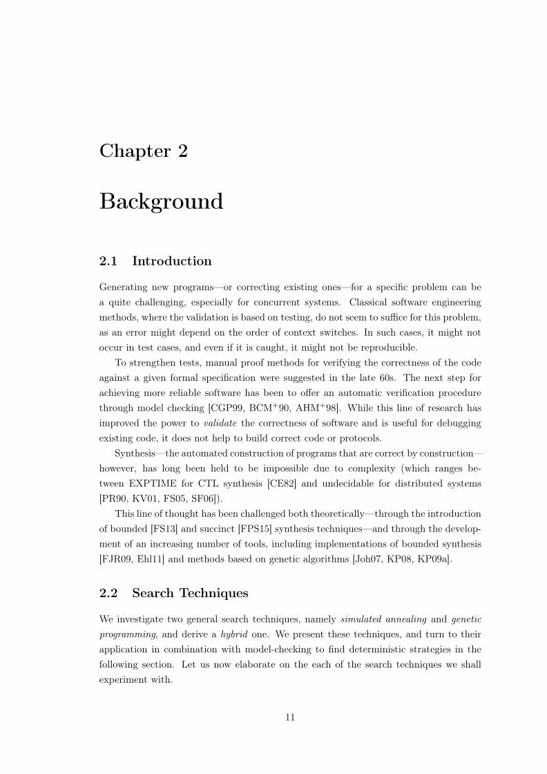
Simulated annealing [CJ01, HJJ03] is a general local search technique that is able toescape from local optima, is easy to implement, and has good convergence properties.When applied to an optimisation problem, the fitness function (objective) generatesvalues for the quality of the solution constructed in each iteration.
The fitness of this newly selected solution is then compared with the fitness of thesolution from the previous round. Improved solutions are always accepted, while some ofthe other solutions are accepted in the hope of escaping local optima in search of globaloptima.
The probability of accepting solutions with reduced fitness depends on a temperatureparameter, which is typically falling monotonically with each iteration of the algorithm.
Figure 2.1: Simulated Annealing Flow Chart
Simulated annealing starts with an initial candidate solution. In each iteration, aneighboring solution is generated by mutating the previous solution. Let, for the ith
iteration, Fi−1 be the fitness of the ‘old’ solution and Fi the fitness of its mutationconstructed in the ith iteration. If the fitness is not decreased (Fi ≥ Fi−1), then themutated solution is kept. If the fitness is decreased (Fi < Fi−1), then the probability p

Chapter 2. Background 13
that this mutated solution is kept is
p = eFi−Fi−1
Ti ,
where Ti is the temperature parameter for the ith step. The chance of changing to amutation with smaller fitness is therefore reduced with an increasing gap in the fitness,but also with a falling temperature parameter. The temperature parameter is positiveand usually non-increasing (0 < Ti ≤ Ti−1). The development of the sequence Ti isreferred to as the cooling schedule and inspired by cooling in the physical world [HJJ03].
Algorithm 1: Simulated Annealing algorithmSet the iteration value i := 0Set the initial temperature T to very high valueloop coolingloop Local searchRandomly derive initial solution xrepeati := i+ 1derive a neighbour solution x′ of x∆F := F (x′)− F (x)if ∆F >= 0 thenx := x′
elsederive random number p ∈ [0, 1]
if p < e∆FT (i) then
x := x′
end ifend ifend loop Local search
until the goal is reached or i = imax
end loop Cooling
The effect of cooling on the simulation of annealing is that the probability of followingan unfavorable move is reduced. In practice, the temperature is often decreased instages. During each stage the temperature is kept constant until a balanced solution isreached. The set of parameters that determines how the temperature is reduced (i.e.,the initial temperature, the stopping criterion, the temperature decrements betweensuccessive stages, and the number of transitions for each temperature value) is calledthe cooling schedule. We have used a simple cooling schedule, where the temperature isdropped by a constant in each iteration. The algorithm is described in Algorithm 1.
2.2.2 Genetic Programming
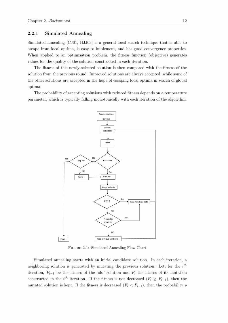
Genetic programming [Koz92] is a different general search technique that has been usedfor program synthesis in a similar setting [Joh07, KP08, KP09a, KP09b]. In geneticprogramming, a population of λ candidate programs is first generated randomly. In each
Chapter 2. Background 14
step, µ candidates (with µ λ) selected from the main popualtion according on theirfitness value.
Figure 2.2: Genetic Programming Flow Chart
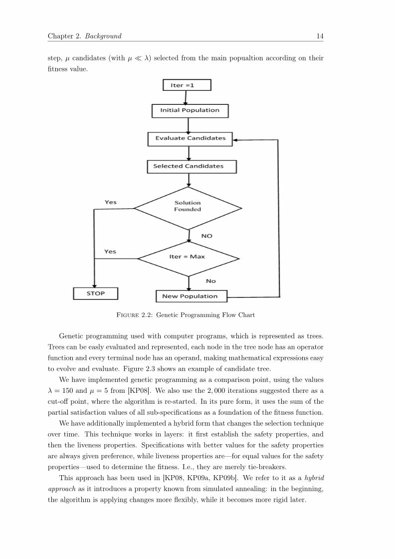
Genetic programming used with computer programs, which is represented as trees.Trees can be easly evaluated and represented, each node in the tree node has an operatorfunction and every terminal node has an operand, making mathematical expressions easyto evolve and evaluate. Figure 2.3 shows an example of candidate tree.
We have implemented genetic programming as a comparison point, using the valuesλ = 150 and µ = 5 from [KP08]. We also use the 2, 000 iterations suggested there as acut-off point, where the algorithm is re-started. In its pure form, it uses the sum of thepartial satisfaction values of all sub-specifications as a foundation of the fitness function.
We have additionally implemented a hybrid form that changes the selection techniqueover time. This technique works in layers: it first establish the safety properties, andthen the liveness properties. Specifications with better values for the safety propertiesare always given preference, while liveness properties are—for equal values for the safetyproperties—used to determine the fitness. I.e., they are merely tie-breakers.
This approach has been used in [KP08, KP09a, KP09b]. We refer to it as a hybridapproach as it introduces a property known from simulated annealing: in the beginning,the algorithm is applying changes more flexibly, while it becomes more rigid later.
Chapter 2. Background 15
*
-
x y
+
z 3
Figure 2.3: GP Candidate Tree
We have implemented the genetic approaches with and without crossover, and usedboth evaluation techniques for simulated annealing, where we refer to using the classicfitness function as a rigid evaluation, and to the hybrid approach as flexible evaluation.
2.2.3 Initialization
The generation of the initial population has a significant effect on the GP performance.Populations with poor diversity may have a negative effect on finding a correct solution.On the otherhand, the initial population size can increase the cost of finding a correctsolution. Initial populations are typically randomly generated. Here, we will describegrow method, which we have used in our work. In the grow method, nodes are takenrandomly from both function and terminal sets until the generator selects enough ter-minals to end the tree or it reaches the maximal depth. The grow method is known toproduce trees of irregular shapes [Koz92]. Similar to the full tree generator, the problemwith the grow method is that the shape of the trees with the grow method is directlyinfluenced by the size of the function and the terminal sets.
2.3 Genetic Operators
2.3.1 Mutation
The main operators of genetic programming are mutation and crossover.Mutation only work with one parent. A mutation point is selected randomlly, the
sub-tree rooted by the selected node replaced by another sub-tree of the same type. Thenew sub-tree is generated randomly. Mutation can also be applied on one node randomlyselected from the leaf or inner nodes. See Figure 2.4 and Figure 2.5.
2.3.2 Crossover
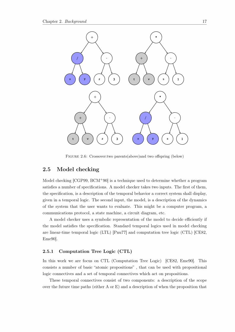
The main aim of crossover Figure 2.6 is to combine the nodes of two parents by exchang-ing some nodes from one parent tree with some from the other. The most commonlyused type of crossover is sub-tree crossover. In sub-tree crossover, the GP system selects

Chapter 2. Background 16
*
-
x y
+
z 3
*
/
x y
+
z 3
Figure 2.4: Candidate tree (left) with one node mutations (right)
*
-
x y
+
z 3
*
/
m n
+
z 3
Figure 2.5: Program tree (left) with sub-tree mutations (right)
two trees. The system randomly selects two crossover points in each parent and swapsthe sub-trees rooted there. Then, it generates a new offspring, which consists of parts ofthe two selected parents [Koz92]. Therefore, the crossover points are selected randomlyand independently.
2.4 Hybrid Genetic Programming
A part from simulated annealing and pure genetic programming with and withoutcrossovers as presented above, we additionally investigate a hybrid form introducinga property known from simulated annealing into the genetic programming algorithm:
by appropriately tuning the measures of fitness, changes are applied more flexibly inthe beginning, while evolution becomes more rigid over time. This hybrid approach hasalready been used for program synthesis by [KP08, KP09a, KP09b] as well as [HS16].
In our case, it basically consists in changing the candidate selection technique overtime, by first establishing the safety properties only, and then the liveness properties.
Just as for the genetic programming technique, crossovers are optional for this hybridapproach as well.
Chapter 2. Background 17
+
/
x y
-
z 3
*
+
t v
-
s 1
+
+
t v
-
z 3
*
/
x y
-
s 1
Figure 2.6: Crossover:two parents(above)and two offspring (below)
2.5 Model checking
Model checking [CGP99, BCM+90] is a technique used to determine whether a programsatisfies a number of specifications. A model checker takes two inputs. The first of them,the specification, is a description of the temporal behavior a correct system shall display,given in a temporal logic. The second input, the model, is a description of the dynamicsof the system that the user wants to evaluate. This might be a computer program, acommunications protocol, a state machine, a circuit diagram, etc.
A model checker uses a symbolic representation of the model to decide efficiently ifthe model satisfies the specification. Standard temporal logics used in model checkingare linear-time temporal logic (LTL) [Pnu77] and computation tree logic (CTL) [CE82,Eme90].
2.5.1 Computation Tree Logic (CTL)
In this work we are focus on CTL (Computation Tree Logic) [CE82, Eme90]. Thisconsists a number of basic “atomic propositions” , that can be used with propositionallogic connectives and a set of temporal connectives which act on propositions.
These temporal connectives consist of two components: a description of the scopeover the future time paths (either A or E) and a description of when the proposition that

Chapter 2. Background 18
Figure 2.7: Model Checking
is the argument of the temporal operator holds within that scope (one of G,F,X or U).These have (in informal terms) the following meanings:
• A The proposition has to hold on All paths starting from the current point.
• E There Exists a path starting from current state on which the proposition willhold.
• G The proposition holds all states (Globally) along the path.
• F The proposition has to hold somewhere (in the Future) along the path.
• X The neXt state the proposition will be satisfied.
• U The proposition holds Until a second proposition holds.
(U is the only binary operator, the others are unary)Given a finite set Π of atomic propositions, the syntax of a CTL formula is defined
as follows:
φ ::= p | ¬φ | φ ∨ φ | Aψ | Eψ,
ψ ::= Xφ | φUφ | Gφ,
where p ∈ Π. For each CTL formula φ we denote the length of φ by |φ|.Let T = (V,E) be an infinite directed tree, with all edges pointing away from the
root. (In model checking, this is the unraveling of the model.) Let l : V → 2Π be alabeling function. The semantics of CTL is defined as follows. For each v ∈ V we have:

Chapter 2. Background 19
• v |= p if, and only if, p ∈ l(v).
• v |= ¬φ if, and only if, v 6|= φ.
• v |= φ ∨ ψ if, and only if, v |= φ or v |= ψ.
• v |= Aψ if, and only if, for all paths π starting at v, we have π |= ψ.
• v |= Eψ if, and only if, there exists a path π starting at v with π |= ψ.
Let π = v1, v2, . . . be an infinite path in T . We have:
• π |= Xφ if, and only if, v2 |= φ.
• π |= φUφ′ if, and only if, there exists an i ∈ N such that vi |= φ′ and, for all j inthe range 1 ≤ j < i, we have vj |= φ.
• π |= Gφ if, and only if, vi |= φ for all i ∈ N.
Note that the φ and φ′ here are state formulas.The pair (T, l), where T is a tree and l is a labeling function, is a model of φ if, and
only if, r |= φ, where r ∈ V is the root of the tree. If (T, l) is a model of φ, then we writeT, l |= φ.
For the candidate programs in our work, the tree is the tree of all runs / interleavingof the programs under asynchronous composition, and the labels are the program states.

Chapter 3
Program Synthesis
This chapter is based on the results of [HS16]. We extend the quest for the best generalsearch technique by studying the effect of the parameter settings for the individual searchtechniques: the influence of the selected temperature for simulated annealing and thecrossover ratio for genetic programming. Note that we have already describe the generalsearching techniques and model checking on Chapter 1.
We start with our tool structure description in section 3.3,that simplify the mainparts of the synthesis tool. Then on section 3.4 we discuss how the model checking usedas a fitness for our searching methods. Section 3.5 shows how the programs representedin two forms for mutation purpose and as a pseudo code. Section 3.6 describes the casestudies that we have solved using the synthesis tool. The investigation of the parametersvariety shown on Section 3.7.1. The rest of the chapter consist of the evaluation section(3.8) and the discussion (section 3.9) of the tool results.
3.1 Abstract
Program synthesis can be viewed as an exploration of the search space of candidate pro-grams in pursuit of an implementation that satisfies a given property. Classic synthesistechniques facilitate exhaustive search, while genetic programming has recently proventhe potential of generic search techniques. But is genetic programming the right searchtechnique for the synthesis problem? In this chapter we challenge this belief and arguein favour of simulated annealing, a different class of general search techniques. We showthat, in hindsight, the success of genetic programming has drawn from what is arguably ahybrid between simulated annealing and genetic programming, and compare the fitnessof classic genetic programming, the hybrid form, and pure simulated annealing. Ourexperimental evaluation suggests that pure simulated annealing offers better results forautomated programming than techniques based on genetic programming.
21

Chapter 3. Program Synthesis 22
3.2 Introduction
Model checking methods are used to verify the correctness of digital circuits and codeagainst their formal specification. In case of design or programming errors, they pro-vide counterexample evidence of erroneous behavior. Model checking techniques sufferfrom inherent high complexity. New model checking methods attempt to speed it upand reduce the memory requirement. Recently, the more ambitious task of convertingthe formal specification automatically into correct-by-design code has gained significantprogress. In this chapter, automata-based techniques for model checking and automaticsynthesis are described.
Concurrent systems are are very difficult to synthesize, where a specific task needs tobe decomposed into many components, where each having limited visibility and controlon the behaviour of the other components. This make the synthesis of concurrent systemsis, in general, undecidable, so the classical software engineering methods in which testingis used for selection seems not suitable for this type of synthesis. The holy grail of suchtechniques would be synthesis: the automated construction of programs that are correctby construction. Such synthesis techniques have long been held to be impossible forreactive systems due to the complexity of synthesis, which ranges from EXPTIME forCTL synthesis [CE82, KV99] to undecidable for distributed systems [PR90, MT01, FS05,SF06].
This line of thought has come under attack on many fronts. On the theoretical side,bounded [FS13] and succinct [FPS15] synthesis techniques have levelled the playing fieldbetween the verification and synthesis of reactive systems by shifting the focus from theinput complexity to the cost measured in the minimal explicit and symbolic solution,respectively. One could argue that this is the theoretical underpinning of successfulapproaches, including implementations of bounded synthesis [FJR09], and methods basedon genetic programming [Joh07, KP08, KP09a, KP09b], also in [Ehl11] Unbeast, a toolfor the synthesis of reactive systems from LTL specifications has presented
The success of genetic programming is also based on the observation that the neigh-borhood of good solutions are often ‘not bad’, and would often still display many soughtafter properties, such as satisfying a number of sub-specifications fully, and others par-tially. Such properties are translated to a high fitness of the candidate solution. Viceversa, the higher the fitness of a candidate, the more likely is it to find a full solution inits proximity. This observation is also at the heart of traditional engineering techniques:usually the elimination of a bug does not cause errors in other places. It is also the as-sumption used when applying program repair [JGB05, vEJ13] techniques. The successivedevelopment into correct programs is also distantly related to counter-example-guidedinductive synthesis [Sol13] for inductive programs, where a genetic approach has alsobeen discussed [DKL15].
Our work is at the same time inspired by the success of genetic programming anddriven by the doubt if genetic programming is the right generic search technique to use.The success of genetic programming for synthesis is thoroughly documented by a series
Chapter 3. Program Synthesis 23
of papers by Katz and Peled [KP08, KP09a, KP09b]. The doubts, on the other hand,are fueled by the general observation that genetic programming is often outperformedby simulated annealing [Dav87, LMST96, MS96].
On a conceptual level, the difference between simulated annealing and genetic pro-gramming techniques are rather minor. These difference are threefold. The first differ-ence is in the number of candidates considered in each iteration. In genetic programming,these are many. In the Katz and Peled papers [KP08, KP09a, KP09b], for example, theseare typically 150, 5 from the previous cycle and 145 mutated programmes—numbers wehave copied for our own experiments with genetic programming. In simulated annealing,there is typically one new implementation in each iteration. The second difference isthat genetic approaches may use crossovers, a proper mix of two candidate solutions, inaddition to mutations, whereas simulated annealing only uses mutations1. The third dif-ference is the way the selection takes place. The rules for selection is typically static forgenetic programming, while the entropy falls over time in simulated annealing. It is im-portant to note that crossovers are not always used in genetic programming, and we arenot aware of any genetic programming approach that has tried to exploit crossovers forsynthesis. Personal communication with the authors of [KP08, KP09a, KP09b] showedthat they did not believe that crossover would be useful in the context of synthesis.
Simulated annealing has been reported [Dav87, LMST96, MS96] to outperform ge-netic programming when crossovers do not provide an advantage or are not used. Broadlyspeaking, this is because keeping only a single instance increases the update speed (wherethe factor is roughly the number of instances), whereas many instances reduce the searchdepth or increase the likelihood of success in a bounded search with a fixed number ofiterations. Overall, the speed-up of the update tends to outweigh the increase in depth,or the reduction in the success rate, of a bounded search. This led us to the hypothesisthat the same holds when these techniques are used in synthesis.
Finally, the paper series on genetic programming by Katz and Peled [KP08, KP09a,KP09b] has used a layered approach, where the evaluation of the search function differsover time, starting with establishing the safety then liveness properties. The effect ofthis difference is comparable to the effect of cooling when a stable level of quality isreached. We took this as another hint that simulated annealing is the more appropriatetechnique when implementing synthesis based on general search with model checkingas a fitness measure. In this work we suggest to use simulated annealing for programsynthesis and compare it to similar approaches based on genetic programming. We usea formal verification technique, model checking, as a way of assessing its fitness in aninductive automatic programming system.
We have implemented a synthesis tool, which uses multiple calls to the model checkerNuSMV [CCG+02] to determine the fitness for a candidate program. The candidateprograms exist in two forms. The main form is a simple imperative language. This form
1The changes are usually not referred to as mutations, but the rules of obtaining them are the same.We use the term mutations for simulated annealing, too, in order to ease the comparison between
simulated annealing and genetic programming.
Chapter 3. Program Synthesis 24
is subject to mutation, but it is translated to a secondary form, the modeling languageof NuSMV, for evaluating its fitness. All choices of how exactly a program is representedand how exactly the fitness is evaluated are disputable.
Generic search techniques are, however, usually rather robust against changes insuch details. While there has been further research on how to measure partial satisfaction[HO13], we believe that the best choice for us is to keep to the choices made for promotinggenetic programming [KP08, KP09a, KP09b], as this is the only choice that is completelyfree of suspicion of being selected for being more suitable for simulated annealing thanfor genetic programming. A second motivation for this selection is that it results in verysimple specifications and, therefore, in fast evaluations of the fitness.
Noting that synthesis entails on average hundreds of thousands to millions of calls toa model checker, only simple evaluations can be considered. We have implemented sixdifferent combinations of selection and update mechanism to test our hypothesis: besidessimulated annealing, we have used genetic programming both without crossover (as dis-cussed in [KP08, KP09a, KP09b]) and with crossover. The tests we have run confirmedthat simulated annealing performs significantly better than genetic programming. As aside result, we found that the assumption of the authors of [KP08, KP09a, KP09b] thatcrossover does not accelerate genetic programming did not prove to be entirely correct,but the advantages we observed were minor.
3.3 The Approach in a Nutshell
Our tool consists of four main components: a modifier / seeder for programs (ProgramGeneration), a compiler into a model checker format (Program Translation), a quantita-tive extension of a model checker, using NuSMV [CCG+02] as a back-end, and a selectorthat determines which program to keep (Generic Search Technique).
The structure of our synthesis tool is shown in Figure 3.1. In a nutshell, our synthe-siser (cf. Figure 3.1) Via a user-interface, the user can select the problem parameters:(1) Search technique; (2) NuSMV specification (3) number, size, and type of variables;and (4) complex or simple conditional statements (if and while statement).
The parameters are sent to the Program Generator, which generates new programs ac-cording to the given parameters. Each program is first translated into NuSMV [CCG+02]and then analysed by NuSMV. The model checking results form the basis of a fitnessfunction for the selected search technique. The specification is provided in form of a listof sub-specifications, which is then automatically extended to additional weaker specifi-cations that are used to obtain a quantitative measure for partial satisfaction.
Broadly speaking, the extension takes partial satisfaction of a specification into ac-count by giving different weights to different weaker versions of sub-specifications (cf.Section 3.4). The result can be manually modified, but the results reported in Section3.8 refer to the automatically produced extension. The internal representation of a pro-gram is a tree. The seeder / modifier produces an initial seed. (Alternatively, one could

Chapter 3. Program Synthesis 25
User Interface
Generator
Translator Fitness MeasureNuSMV
Search Technique
parameters properties
Candidate tree
Model Output
properties Fitness
Output
candidate update
Figure 3.1: Synthes Tool
start with an initial program provided by the user.) The modifier / seeder also producesmodifications of existing programs by changing sub-trees (cf. Section 3.5). The programsare then translated to the input language of a model checker (NuSMV in our case), whichis then called several times to determine the level of satisfaction, which is the measureof the fitness (cf. Section 3.3) of a program.
Broadly speaking, the number of candidate programs kept depends on the search tech-nique used. We have implemented both genetic programming approaches and simulatedannealing in order to obtain a clean point of comparison. We use NuSMV [CCG+02] as amodel checker. The translator therefore translates the abstract programs into the modellanguage of NuSMV. The other parts of the tool are written in C++. Figure 3.1 gives anoverview on the main components of our tool. When comparing simulated annealing togenetic programming, we merely replace the simulated annealing component by a similarcomponent for the respective genetic programming variant and optionally add crossoverto the available mutations.
The user provides specifications for the desired properties of a system in the formof a list of CTL specifications for the system dynamics that the program has to satisfy.The simulated annealing component then derives the intermediate specifications (full andpartial compliance) that are used to determine the fitness of a candidate (cf. Section 3.3).If the candidate program satisfied all required properties, then the synthesiser returns itas a correct program.
Otherwise, it will compare the fitness of the current candidate with the (stored)fitness value of the program it is derived from by mutation. (This is the currently storedcandidate.) If the fitness is lower, then the tool will update the stored candidate withthe probability e∆F/T (i) defined by the loss ∆F = Fi − Fi−1 in fitness and the currenttemperature T (i) taken from the cooling schedule.

Chapter 3. Program Synthesis 26
If the fitness is not lower, the tool will always replaces the stored candidate by themutated one. When the end of the cooling schedule is reached, the tool aborts. Thesynthesis process is then re-started, either with a fresh cooling schedule (usually with ahigher starting temperature or slower cooling) or with the same cooling schedule. Wehave implemented the latter.
3.4 Model Checking as a Fitness Function
We use model checking to determine the fitness of a candidate program in the same wayas it has been used for genetic programming [KP08, KP09a, KP09b]. Based on the modelchecking results, we derive a quantitative measure for the fitness (as a level of partialcorrectness) of a program. This can be the share of properties that are satisfied so far,or mechanically produced simpler properties.
For example, if a property shall hold on all paths, it is better if it holds on some paths,and yet better if it holds almost surely. Our implementation considers the specificationas a list of sub-specifications and assigns full marks for each sub-specification, which issatisfied by the candidate program. For cases where the sub-specification is not satisfied,we distinguish between different levels of partial satisfaction. We offer an automatedtranslation of properties with up to two universal quantifiers that occur positively. Toevaluate the candidates 100 points are assigned when the sub-specification is satisfied, 80
points if the specification is satisfied when replacing one universal path quantifier by anexistential path quantifier, and 10 points are assigned if the specification is satisfied afterreplacing both universal path quantifiers by existential ones. Those evaluation numbersare given to weight the candidates and distinguish among three levels of them accordingto the satisfaction of the specifications. This means that it is possible to take anothervalues (eg. 20, 60, and 100) the most important thing is keep the difference among themclear. (Existential quantifiers that occur negatively are treated accordingly.) Examplesof this automated translation are shown in Section 3.6.
The output of the model checker is used to evaluate the fitness of the current candi-date. The main part of the fitness is the average of the values for all sub-specifications inthe rigid evaluation and the average of all liveness specifications in the flexible evaluation.Following [KP08], we apply a penalty for long programs by deducing the number of innernodes of a program from this average when assigning the fitness of a candidate program.The resulting fitness value will be used by simulated annealing to compare the currentcandidate with the previous one when using rigid evaluation, and to make a decisionwhether the changes will be preserved or discarded. When using flexible evaluation, thisonly happens if the value for the safety specification is equal; falling resp. rising valuesfor safety specifications always result in discarding resp. selecting the update when usingflexible evaluation.
Chapter 3. Program Synthesis 27
while
==
turn me
=
other 0
while
!=
turn me
=
other 0
Figure 3.2: Program tree (left) with one node mutations (right)
while
==
turn me
=
other 0
while
!=
me 0
=
other 0
Figure 3.3: Program tree (left) with sub-tree mutations (right)
3.5 Programs as Trees
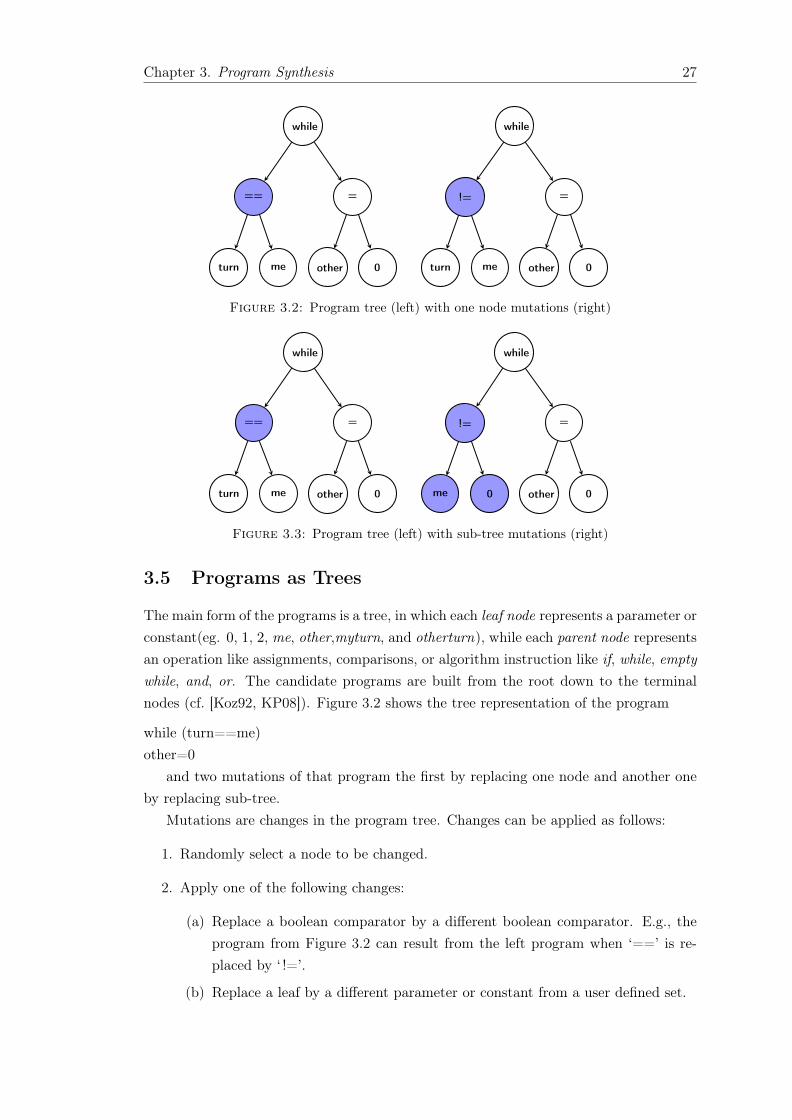
The main form of the programs is a tree, in which each leaf node represents a parameter orconstant(eg. 0, 1, 2, me, other,myturn, and otherturn), while each parent node representsan operation like assignments, comparisons, or algorithm instruction like if, while, emptywhile, and, or. The candidate programs are built from the root down to the terminalnodes (cf. [Koz92, KP08]). Figure 3.2 shows the tree representation of the program
while (turn==me)other=0
and two mutations of that program the first by replacing one node and another oneby replacing sub-tree.
Mutations are changes in the program tree. Changes can be applied as follows:
1. Randomly select a node to be changed.
2. Apply one of the following changes:
(a) Replace a boolean comparator by a different boolean comparator. E.g., theprogram from Figure 3.2 can result from the left program when ‘==’ is re-placed by ‘ !=’.
(b) Replace a leaf by a different parameter or constant from a user defined set.
Chapter 3. Program Synthesis 28
While
==
turn me
=
other 0
While
!=
turn other
=
me 1
While
!=
turn other
=
other 0
while
==
turn me
=
me 1
Figure 3.4: Crossover:two parents(above)and two offspring (below)
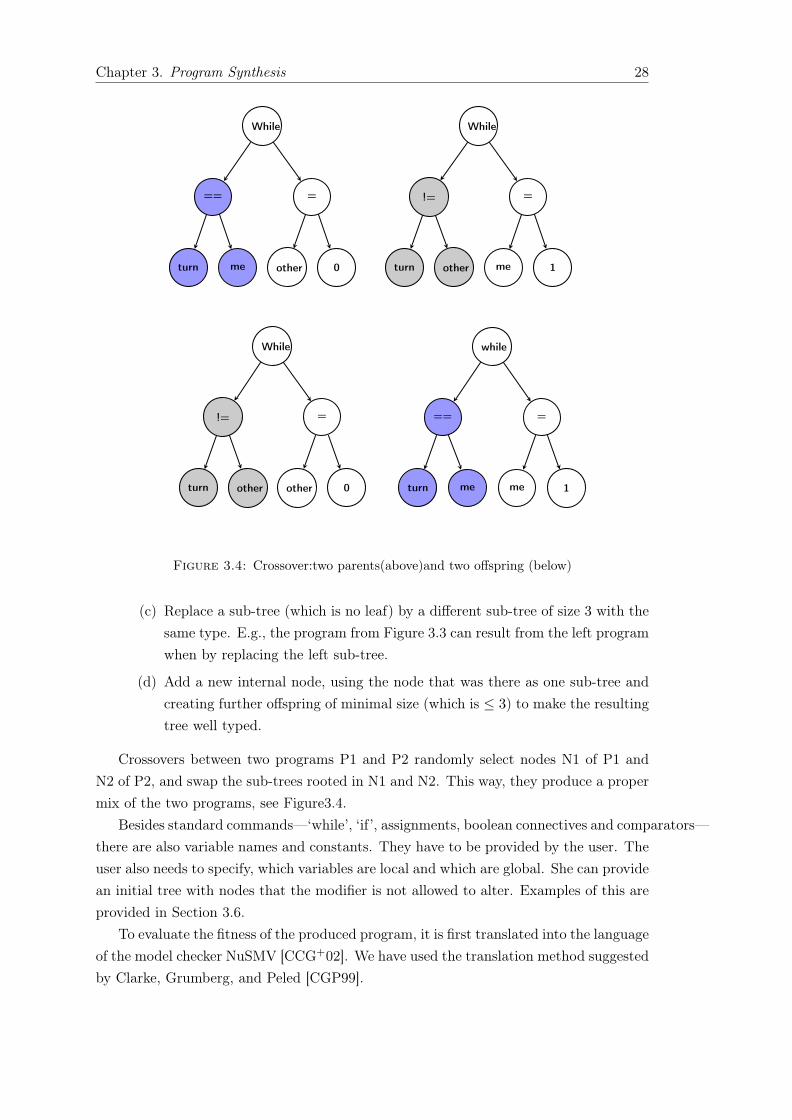
(c) Replace a sub-tree (which is no leaf) by a different sub-tree of size 3 with thesame type. E.g., the program from Figure 3.3 can result from the left programwhen by replacing the left sub-tree.
(d) Add a new internal node, using the node that was there as one sub-tree andcreating further offspring of minimal size (which is ≤ 3) to make the resultingtree well typed.
Crossovers between two programs P1 and P2 randomly select nodes N1 of P1 andN2 of P2, and swap the sub-trees rooted in N1 and N2. This way, they produce a propermix of the two programs, see Figure3.4.
Besides standard commands—‘while’, ‘if’, assignments, boolean connectives and comparators—there are also variable names and constants. They have to be provided by the user. Theuser also needs to specify, which variables are local and which are global. She can providean initial tree with nodes that the modifier is not allowed to alter. Examples of this areprovided in Section 3.6.
To evaluate the fitness of the produced program, it is first translated into the languageof the model checker NuSMV [CCG+02]. We have used the translation method suggestedby Clarke, Grumberg, and Peled [CGP99].

Chapter 3. Program Synthesis 29
process mewhile (true) dononcritical sectionwhile (turn==me) doskip
end whilecritical sectionturn=other
end while
‘me’ and ‘other’ are (differ-ent) variable valuations, inthis example implemented asboolean variables. In otherinstances, they might be havea different (finite) datatype.
MODULE p(turn)VARpc: 11, 12, 14,15;ASSIGNinit(pc) := 11;next(pc) :=case(pc=11) : 11, 12;(pc=12)&(turn=me) : 14;
(pc=14) : 15;(pc=15) : 11;TRUE: pc;esac;next(turn):=case(pc=15): other;TRUE :turn;esac;
Figure 3.5: Translation example – source(left) and target (right)
In this translation, the program is converted into very simple statements (similar toassembly language). To simplify the translation, the program lines are first labeled, andthis label is then uses as a pointer that represents the program counter (PC). From thisintermediate language, the NuSMV model is then built by creating (case) and (next)statements that use the PC. Figure 3 shows the translation of a mutual exclusion algo-rithm. At first, each line in the source algorithm labelled, then a variable pc (which islocal for each MODULE) is added to represent the control state.
In the first step label each statement in the algorithm, the labels will used to buildthe model.
First step label the statements
10 while (true)11 noncritical section12 while (turn==0)13 skip14 critical section15 turn=1
The next step is adding a pointer variable pc, and define all the variables as globalvariables.
Second add pc variableVARturn:boolean;

Chapter 3. Program Synthesis 30
p0:process(turn,myturn);p1:process(turn,myturn);....MODULE P(turn,myturn)VARpc: 11, 12, 14,15;10 while (true)11 noncritical section12 while (turn==0)13 skip14 critical section15 turn=1
Finally build the case and next state expression according the values of pc variable.
Thired Initialize all the variables properly, and start building their next-stateexpressions:MODULE p(turn, myturn)VARpc: 11, 12, 14,15;ASSIGNinit(pc) := 11;next(pc) :=case(pc=11) : 11, 12;(pc=12)&(turn=myturn) : 14;(pc=14) : 15;(pc=15) : 11;TRUE: pc;esac;next(turn):=case(pc=15): !myturn;TRUE :turn;esac;
And so on until build all the case statements by adding clauses according to thealgorithm fragments, til create the program.
Chapter 3. Program Synthesis 31
3.6 Case Studies
We have selected mutual exclusion [Dij65] and leader election [LP85, KP09b] as casestudies, because these are the examples, for which genetic programming has been suc-cessfully attempted. In mutual exclusion, the programming language is set to use twoand three shared bits, and for leader election 3 and 4 nodes ring can be used.
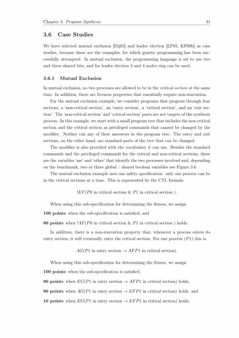
3.6.1 Mutual Exclusion
In mutual exclusion, no two processes are allowed to be in the critical section at the sametime. In addition, there are liveness properties that essentially require non-starvation.
For the mutual exclusion example, we consider programs that progress through foursections, a ‘non-critical section’, an ‘entry section’, a ‘critical section’, and an ‘exit sec-tion’. The ‘non-critical section’ and ‘critical section’ parts are not targets of the synthesisprocess. In this example, we start with a small program tree that includes the non-criticalsection and the critical section as privileged commands that cannot be changed by themodifier. Neither can any of their ancestors in the program tree. The entry and exitsections, on the other hand, are standard parts of the tree that can be changed.
The modifier is also provided with the vocabulary it can use. Besides the standardcommands and the privileged commands for the critical and non-critical sections, theseare the variables ‘me’ and ‘other’ that identify the two processes involved and, dependingon the benchmark, two or three global / shared boolean variables see Figure 3.6.
The mutual exclusion example uses one safety specification: only one process can bein the critical sections at a time. This is represented by the CTL formula
!EF (P0 in critical section & P1 in critical section ).
When using this sub-specification for determining the fitness, we assign
100 points when the sub-specification is satisfied, and
80 points when !AF (P0 in critical section & P1 in critical section ) holds.
In addition, there is a non-starvation property that, whenever a process enters itsentry section, it will eventually enter the critical section. For one process (P1) this is
AG(P1 in entry section→ AFP1 in critical section).
When using this sub-specification for determining the fitness, we assign
100 points when the sub-specification is satisfied,
80 points when EG(P1 in entry section→ AFP1 in critical section) holds,
80 points when AG(P1 in entry section→ EFP1 in critical section) holds, and
10 points when EG(P1 in entry section→ EFP1 in critical section) holds.
Chapter 3. Program Synthesis 32
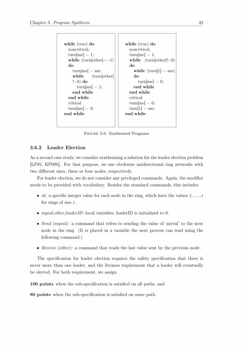
while (true) dononcritical;turn[me] = 1;while (turn[other]==1)doturn[me] = me;while (turn[other]!=0) doturn[me] = 1;
end whileend whilecriticalturn[me] = 0;
end while
while (true) dononcritical;turn[me] = 1;while (turn[other]!=0)dowhile (turn[1]==me)doturn[me] = 0;
end whileend whilecriticalturn[me] = 0;turn[1] = me;
end while
Figure 3.6: Synthesized Programs
3.6.2 Leader Election
As a second case study, we consider synthesising a solution for the leader election problem[LP85, KP09b]. For that purpose, we use clockwise unidirectional ring networks withtwo different sizes, three or four nodes, respectively.
For leader election, we do not consider any privileged commands. Again, the modifierneeds to be provided with vocabulary. Besides the standard commands, this includes
• id: a specific integer value for each node in the ring, which have the values 1, . . . , i
for rings of size i.
• myval,other,leaderID: local variables; leaderID is initialized to 0.
• Send (myval): a command that refers to sending the value of ‘myval’ to the nextnode in the ring. (It is placed in a variable the next process can read using thefollowing command.)
• Receive (other): a command that reads the last value sent by the previous node.
The specification for leader election requires the safety specification that there isnever more than one leader, and the liveness requirement that a leader will eventuallybe elected. For both requirement, we assign
100 points when the sub-specification is satisfied on all paths, and
80 points when the sub-specification is satisfied on some path.

Chapter 3. Program Synthesis 33
3.7 Synthesis Approach
When using the tool, the user starts with determining the search technique s/he wouldlike to use from a list of three types of the techniques:
genetic programming, hybrid, and simulated annealing. Both the genetic program-ming and the hybrid method can be used with or without crossover. Hybrid [KP09a] isa method, where the fitness is viewed as a pair of ‘safety-fitness’ and ‘liveness-fitness’,where the latter is only used if the safety fitness is equal. For simulated annealing thereare also two flavours to choose from: rigid (where the classic fitness function is used asdescribed above) and flexible, which uses the two-step fitness approach from ‘hybrid’.The tool allows the user to input parameters that control the dynamics of the synthesisprocess. These parameters depend on the selected search technique.
For genetic programming and the hybrid approach, the parameters include the pop-ulation size, the number of selected candidates, and the number of iterations. For simu-lated annealing, the user chooses the initial temperature and the cooling schedule. Theinput specification should be a list of NuSMV specifications. The tool will produceweaker specifications for the purpose of producing a fitness measure.
Finally, the user defines the signature of the program by selecting input variablesthat are used to build the pseudo code of the program that the user want to synthesize.The model checker NuSMV is used for the individual model checking tasks. When thecandidate program satisfies all required properties, the synthesiser returns it as a correctprogram. Otherwise, it will compare the fitness of the current candidate/s with the(stored) fitness value of the program/s it is derived from by mutation. (This is thecurrently stored candidate or population.) The selection of the candidate / populationto be kept is determined by the selected generic search technique.
For simulated annealing, if the fitness is lower, then the tool will update the storedcandidate with the probability defined by the loss in fitness and the current temperaturetaken from the cooling schedule. If the fitness is not lower, the tool will always replacesthe stored candidate by the mutated one. When the end of the cooling schedule isreached, the tool aborts.
3.7.1 Parameters Setting
The tool allows the user to select the generic search technique and to influence theparameter used for fine-tuning the respective technique. The parameters of the searchtechnique determine the likelihood of finding a correct program in each iteration as well asthe expected running time for each iteration. The selected parameters therefore heavilyinfluence the expected overall speed of the search.
The type of available parameters differs between genetic programming and simulatedannealing. Figure 3.7 shows the graphical user interface of the tool, which the user canuse to set the parameters or use the default setting.

Chapter 3. Program Synthesis 34
First, the search technique is selected. The tool then provides the input variablesto input their values, like population size and the number of the selected candidatesfor genetic programming and the hybrid technique, or the initial temperature and thecooling schedule for simulated annealing.
The user can also select the ratio of crossover vs mutation in genetic techniques. Asa default setting, this ratio is 20% and the initial population size is 150 and 5 selectedcandidates.
Figure 3.7: Graphical User Interface
The user should input her list of specifications and define the search space by selectingthe input language (variables and their range). When the tool has found a correctprogram, it is provided to the user.
3.7.2 Temperature Range
Besides serving as a synthesis tool, the main intention of the tool is to allow for a com-parison of different generic search techniques. In [HS16], we have used our technique togenerate correct solutions for mutual exclusion and leader election and found that simu-lated annealing is much (1.5 to 2 orders of magnitude) faster than genetic programming.
In order to test if the hypothesis from [Con90] that simulated annealing does mostof its work during the middle stages—while being in a good temperature range—holdsfor our application, we have developed the tool to allow for ‘cooling schedules’ that donot cool at all, but use a constant temperature. In order to be comparable to the defaultstrategy, we use up to 25, 001 iterations in each attempt.
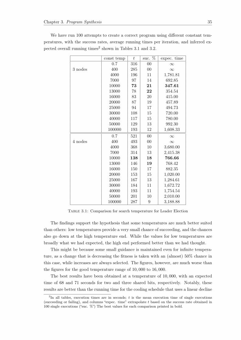
Chapter 3. Program Synthesis 35
We have run 100 attempts to create a correct program using different constant tem-peratures, with the success rates, average running times per iteration, and inferred ex-pected overall running times2 shown in Tables 3.1 and 3.2.
const temp t suc. % expec. time
3 nodes0.7 316 00 ∞400 285 00 ∞4000 196 11 1,781.817000 97 14 692.8510000 73 21 347.6113000 78 22 354.5416000 83 20 415.0020000 87 19 457.8925000 94 17 494.7330000 108 15 720.0040000 117 15 780.0050000 129 13 992.30100000 193 12 1,608.33
4 nodes0.7 521 00 ∞400 493 00 ∞4000 368 10 3,680.007000 314 13 2,415.3810000 138 18 766.6613000 146 19 768.4216000 150 17 882.3520000 153 15 1,020.0025000 167 13 1,284.6130000 184 11 1,672.7240000 193 11 1,754.5450000 201 10 2,010.00100000 287 9 3,188.88
Table 3.1: Comparison for search temperature for Leader Election
The findings support the hypothesis that some temperatures are much better suitedthan others: low temperatures provide a very small chance of succeeding, and the chancesalso go down at the high temperature end. While the values for low temperatures arebroadly what we had expected, the high end performed better than we had thought.
This might be because some small guidance is maintained even for infinite tempera-ture, as a change that is decreasing the fitness is taken with an (almost) 50% chance inthis case, while increases are always selected. The figures, however, are much worse thanthe figures for the good temperature range of 10, 000 to 16, 000.
The best results have been obtained at a temperature of 10, 000, with an expectedtime of 68 and 71 seconds for two and three shared bits, respectively. Notably, theseresults are better than the running time for the cooling schedule that uses a linear decline
2In all tables, execution times are in seconds; t is the mean execution time of single executions(succeeding or failing), and columns “expec. time” extrapolate t based on the success rate obtained in100 single executions (“suc. %”) The best values for each comparison printed in bold.

Chapter 3. Program Synthesis 36
const temp t suc. % expec. time
2 shared bits0.7 147 00 ∞400 143 00 ∞4000 129 3 43007000 77 12 641.610000 15 22 68.1813000 16 23 69.5616000 17 21 80.9520000 21 20 10525000 23 19 121.0530000 28 18 155.5540000 31 16 193.7550000 37 15 246.66100000 52 11 472.72
3 shared bits0.7 155 00 ∞400 148 00 ∞4000 121 4 30257000 81 11 25210000 17 24 70.8313000 18 24 7516000 19 22 86.3620000 23 22 104.5425000 25 21 191.0430000 30 19 157.8940000 34 17 20050000 41 16 256.25100000 58 13 446.15
Table 3.2: Comparison for search temperature for Mutual Exclusion
in the temperature. Starting at 20, 000 and terminating at 0, it has the same averagetemperature.
In the light of the results from the second experiment, it seems likely that the lastthird of the improvement cycles in this cooling schedule had little avail.
3.7.3 Crossover Ratio
Similarly, we have studied the effect of changing the share between crossover and muta-tion in genetic programming.We considered a range from a 0% to 60% share of crossovers.Country to our expectation, we did not observe any relevant effect of in- or decreasingthe share of cross over for either classic or hybrid genetic programming. Interestingly,the running time per instance increased with the share of crossovers, which might pointto a production of more complex programs. See Tables 3.3 and 3.4.
3.7.4 Initial Population Size Cost
The population size affect the algorithm in two sides, firstly large size could provide abetter diversity than the small one, but besides that it could make the algorithm make

Chapter 3. Program Synthesis 37
ratio % t suc. % expec. time
2 shared bits0 583 7 8,328.5720 589 9 6,544.4440 602 9 6,688.8860 614 8 7,657.0080 613 8 7,662.50100 652 2 32,600.00
3 shared bits0 615 7 8,785.7120 620 9 6,888.8840 637 9 7,077.7760 658 8 8,225.0080 669 4 16,725.00100 682 2 34,100.00
3 nodes0 1120 3 37,333.3320 1123 6 18,716.6640 1137 5 22,740.0060 1149 5 22,980.0080 1154 3 38,466.66100 1167 2 58,350.00
4 nodes0 1,311 3 43,700.0020 1,314 5 26,280.0040 1,325 4 33,125.0060 1,336 3 44,533.3380 1,345 3 44,833.33100 1,353 2 67,650.00
Table 3.3: Crossover ratio for GP (Program Synthesis)
more computation to find a good solution. In order to investigate how the populationsize effect on our synthesis approach and check the cost of the large size, we initiate thepopulation size to different sizes see Tables 3.5 and 3.6.
We found that the the cost of the initial population size increase the cost of findinga good solution dramatically as shown on Figure 3.8.
3.8 Evaluation
We have implemented the simulated annealing and genetic programming algorithms asdescribed, using NuSMV [CCG+02] as a solver when deriving the fitness of candidateprograms. For simulated annealing, we have set the initial temperature to 20, 000. Thecooling schedule decreases the temperature by 0.8 in each iteration.
The schedule ends after 25, 000 iterations, when the temperature hits 0. In a failedexecution, this leads to determining the fitness of 25, 001 candidate programs.
As described in Section 3.2, we have taken the values suggested in [KP08] for geneticprogramming: λ = 150 candidate programs are considered in each step, µ = 5 are kept,and we abort after 2, 000 iterations. In a failed execution, this leads to determining thefitness of 290, 150 candidate programs.
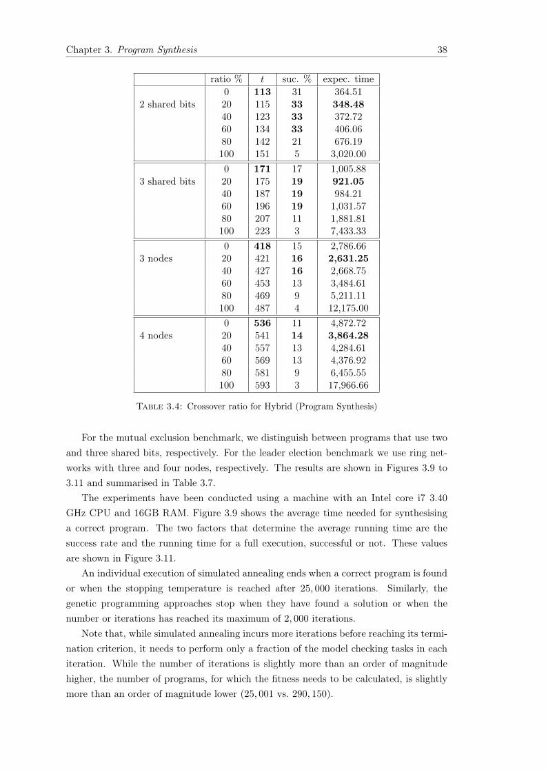
Chapter 3. Program Synthesis 38
ratio % t suc. % expec. time
2 shared bits0 113 31 364.5120 115 33 348.4840 123 33 372.7260 134 33 406.0680 142 21 676.19100 151 5 3,020.00
3 shared bits0 171 17 1,005.8820 175 19 921.0540 187 19 984.2160 196 19 1,031.5780 207 11 1,881.81100 223 3 7,433.33
3 nodes0 418 15 2,786.6620 421 16 2,631.2540 427 16 2,668.7560 453 13 3,484.6180 469 9 5,211.11100 487 4 12,175.00
4 nodes0 536 11 4,872.7220 541 14 3,864.2840 557 13 4,284.6160 569 13 4,376.9280 581 9 6,455.55100 593 3 17,966.66
Table 3.4: Crossover ratio for Hybrid (Program Synthesis)
For the mutual exclusion benchmark, we distinguish between programs that use twoand three shared bits, respectively. For the leader election benchmark we use ring net-works with three and four nodes, respectively. The results are shown in Figures 3.9 to3.11 and summarised in Table 3.7.
The experiments have been conducted using a machine with an Intel core i7 3.40GHz CPU and 16GB RAM. Figure 3.9 shows the average time needed for synthesisinga correct program. The two factors that determine the average running time are thesuccess rate and the running time for a full execution, successful or not. These valuesare shown in Figure 3.11.
An individual execution of simulated annealing ends when a correct program is foundor when the stopping temperature is reached after 25, 000 iterations. Similarly, thegenetic programming approaches stop when they have found a solution or when thenumber or iterations has reached its maximum of 2, 000 iterations.
Note that, while simulated annealing incurs more iterations before reaching its termi-nation criterion, it needs to perform only a fraction of the model checking tasks in eachiteration. While the number of iterations is slightly more than an order of magnitudehigher, the number of programs, for which the fitness needs to be calculated, is slightlymore than an order of magnitude lower (25, 001 vs. 290, 150).
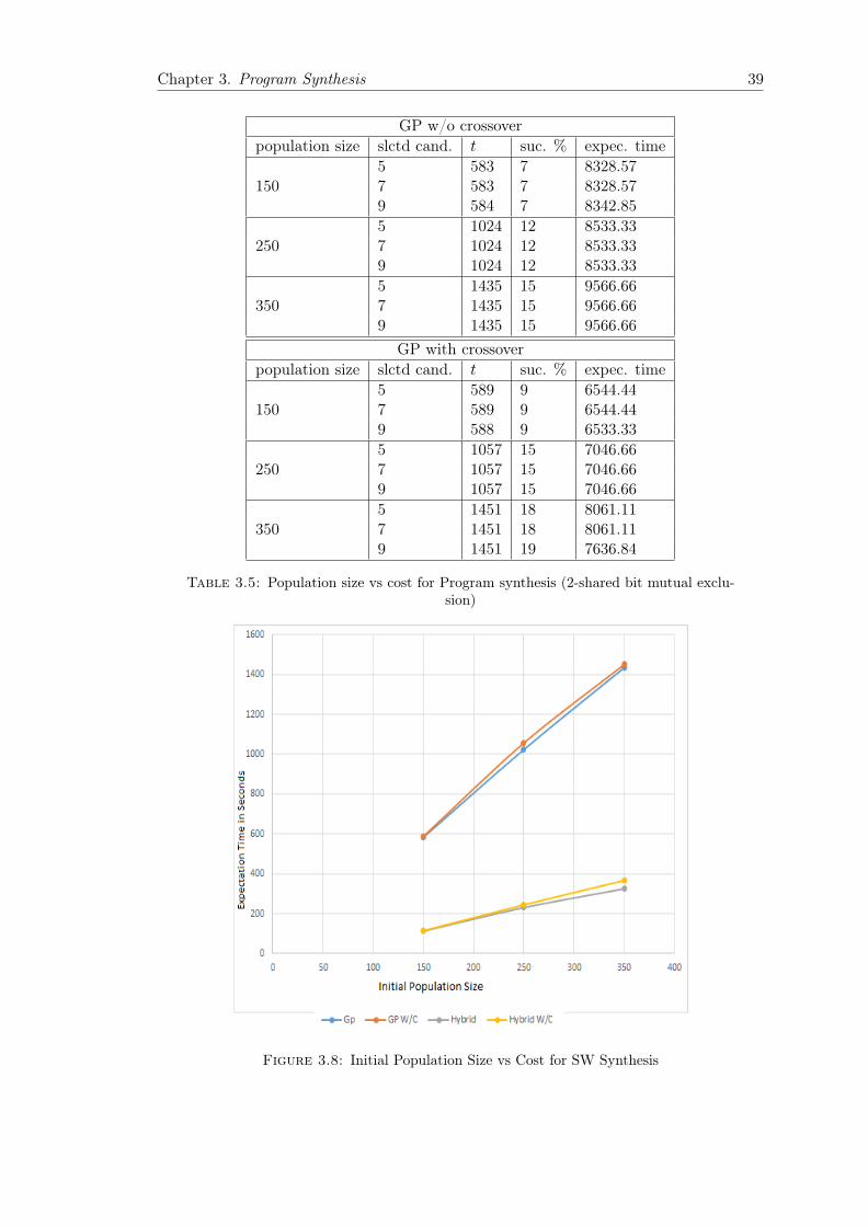
Chapter 3. Program Synthesis 39
GP w/o crossoverpopulation size slctd cand. t suc. % expec. time
1505 583 7 8328.577 583 7 8328.579 584 7 8342.85
2505 1024 12 8533.337 1024 12 8533.339 1024 12 8533.33
3505 1435 15 9566.667 1435 15 9566.669 1435 15 9566.66
GP with crossoverpopulation size slctd cand. t suc. % expec. time
1505 589 9 6544.447 589 9 6544.449 588 9 6533.33
2505 1057 15 7046.667 1057 15 7046.669 1057 15 7046.66
3505 1451 18 8061.117 1451 18 8061.119 1451 19 7636.84
Table 3.5: Population size vs cost for Program synthesis (2-shared bit mutual exclu-sion)
Figure 3.8: Initial Population Size vs Cost for SW Synthesis
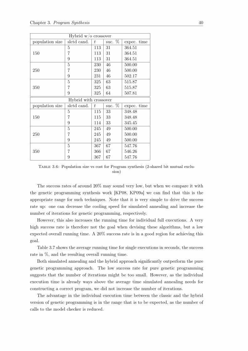
Chapter 3. Program Synthesis 40
Hybrid w/o crossoverpopulation size slctd cand. t suc. % expec. time
1505 113 31 364.517 113 31 364.519 113 31 364.51
2505 230 46 500.007 230 46 500.009 231 46 502.17
3505 325 63 515.877 325 63 515.879 325 64 507.81Hybrid with crossover
population size slctd cand. t suc. % expec. time
1505 115 33 348.487 115 33 348.489 114 33 345.45
2505 245 49 500.007 245 49 500.009 245 49 500.00
3505 367 67 547.767 366 67 546.269 367 67 547.76
Table 3.6: Population size vs cost for Program synthesis (2-shared bit mutual exclu-sion)
The success rates of around 20% may sound very low, but when we compare it withthe genetic programming synthesis work [KP08, KP09a] we can find that this is theappropriate range for such techniques. Note that it is very simple to drive the successrate up: one can decrease the cooling speed for simulated annealing and increase thenumber of iterations for genetic programming, respectively.
However, this also increases the running time for individual full executions. A veryhigh success rate is therefore not the goal when devising these algorithms, but a lowexpected overall running time. A 20% success rate is in a good region for achieving thisgoal.
Table 3.7 shows the average running time for single executions in seconds, the successrate in %, and the resulting overall running time.
Both simulated annealing and the hybrid approach significantly outperform the puregenetic programming approach. The low success rate for pure genetic programmingsuggests that the number of iterations might be too small. However, as the individualexecution time is already ways above the average time simulated annealing needs forconstructing a correct program, we did not increase the number of iterations.
The advantage in the individual execution time between the classic and the hybridversion of genetic programming is in the range that is to be expected, as the number ofcalls to the model checker is reduced.

Chapter 3. Program Synthesis 41
SA rigid SA flexible hybrid hybrid + CO GP GP + CO0
5,000
10,000
15,000
20,000
25,000
30,000
35,000
40,000
45,000
Individu
alexcution
timein
second
s2 shared bits3 shared bits3 nodes4 nodes
Figure 3.9: Average time required for synthesising a correct program
SA rigid SA flexible hybrid hybrid + CO GP GP + CO0
200
400
600
800
1,000
1,200
1,400
Individu
alexcution
timein
second
s
2 shared bits3 shared bits3 nodes4 nodes
Figure 3.10: Average running time of an individual execution

Chapter 3. Program Synthesis 42
SA rigid SA flexible hybrid hybrid + CO GP GP + CO0
5
10
15
20
25
30
35
Individu
alexecutiontimein
second
s
2 shared bits3 shared bits
3 nodes4 nodes
Figure 3.11: success rate of individual executions
It is interesting to note that simulated annealing, where the shift from rigid to flexibleevaluation might be expected to have a similar effect, does not benefit to the same extent.It is also interesting to note that the execution time suggests that determining the fitnessof programs produced by simulated annealing is slightly more expensive.
This was to be expected, as the average program length grows over time. The penaltyfor longer programs reduces this effect, but cannot entirely remove it. (This potentialdisadvantage is the reason why an occasional re-start provides better results than pro-longing the search.)
The advantage in running of simulated annealing compared to the hybrid approachreach from factor 4 to factor 10, and the comparison to pure genetic programming reachfrom factor 35 to factor 76. It is interesting to note that both the pure and the hybridapproach to genetic programming benefit from crossovers, but while the benefit for thepure approach is significant, almost halving the average time for synthesising a programin one case, the benefit for the superior hybrid approach is small.
3.9 Discussion
We have implemented an automated programming technique based on simulated anneal-ing and genetic programming, both in the pure form of [Joh07] and the arguably hybridform of [KP08, KP09a]. The implementations from these papers were unavailable forcomparison, but this is, in our view, a plus:

Chapter 3. Program Synthesis 43
Table 3.7: Search Techniques Comparison
Search Technique t suc. % expec. time
2 shared bitsSA rigid 20 19 105.26
SA flexible 18 21 85.71Hybrid w/o crossover 113 31 364.51Hybrid with crossover 115 33 348.48GP w/o crossover 583 7 8,328.57GP with crossover 589 9 6,544.44
3 shared bitsSA rigid 23 23 100
SA flexible 20 22 90.9Hybrid w/o crossover 171 17 1,005.88Hybrid with crossover 175 19 921.05GP w/o crossover 615 7 8,785.71GP with crossover 620 9 6,888.88
3 nodesSA rigid 84 19 442.1
SA flexible 81 20 405Hybrid w/o crossover 418 15 2,786.66Hybrid with crossover 421 16 2,631.25GP w/o crossover 1120 3 37,333.33GP with crossover 1123 6 18,716.66
4 nodesSA rigid 145 17 852.94
SA flexible 138 18 766.66Hybrid w/o crossover 536 11 4,872.72Hybrid with crossover 541 14 3,864.28GP w/o crossover 1311 3 43,700.00GP with crossover 1314 5 26,280.00
The performance is naturally sensitive to the quality of the integration, the suitabilityof the model checker used, and hidden details, like how the seed is chosen or details ofhow the fitness is computed. The integrated comparison makes sure that all methodsare on equal footage in these regards.
The results are very clear and in line with the expectation we had drawn from theliterature [Dav87, LMST96, MS96]. When crossovers are not used, the main differencebetween the established genetic programming techniques and simulated annealing is thesearch strategy of using many and using a single instance, respectively. The data gatheredconfirms that an increase of the number of iterations can easily overcompensate thebroader group of candidates kept in genetic programming.
Chapter 3. Program Synthesis 44
In our experiments, we have used an increase that fell short of creating the same ex-pected running time for a single full execution (with or without success), and yet outper-formed even the hybrid approach w.r.t. the success rate on three of our four benchmarks.
We have also added variations of genetic programming that include crossover tovalidate the assumption that crossovers do not lead to an annihilation of the advantage,but it proved that the hybrid approach, and thus the stronger competitor, does notbenefit much from using crossover.
The double advantage of shorter running time and higher success rate led to animprovement of 1.5 to 2 orders of magnitude compared to pure genetic programming(with and without crossover), and between half an order and one order of magnitudewhen compared to the hybrid approach (with or without crossover).
The results from in this chapter indicate that simulated annealing is the better generalsearch technique to use. It will be interesting to see if that these factors are essentiallyconstant, or if they depend heavily on the circumstances.
Together with the later extensions, the evaluation with the tool indicates that thereare good temperature ranges. To developing the tool further will be an integration ofthese results into the cooling schedule. One way to do this could, for example, be to chosea temperature, where many improvements have clustered in the observed runs, or just toprogress more slowly through areas where this has been the case during the observed runsin the past. Another possibility to use the observation that some temperatures providebetter results than others could be to re-heat a bit after observing an improved fitness,or to staying in the temperature where this improvement was realised for a while.

Chapter 4
Discrete Controller Synthesis
This chapter is mainly based on the results from [HBS17]. In this chapter we formallydefine the symbolic model and DCS problems, and detail the particular kind of solutionswe seek in Section 4.3.
We then turn to a description of the general search techniques that we investigatein Section 4.5.1, and further detail how we adapted them for solving our symbolic DCSproblems in Section 4.6.
We detail our experiments of our simulated annealing algorithm in Sections 4.7. Weeventually summarise and discuss our results in Section 4.8.4.
4.1 Abstract
Several general search techniques such as genetic programming and simulated annealinghave recently been investigated for synthesising programs from specifications of desiredobjective behaviours.
In this context, these techniques explore the space of all candidate programs byperforming local changes to candidates selected by means of a measure of their fitnesswrt the desired objectives. Previous performance results advocated the use of simulatedannealing over genetic programming for such problems.
In this chapter, we investigate the application of these techniques for the compu-tation of deterministic strategies solving symbolic Discrete Controller Synthesis (DCS)problems, where a model of the system to control is given along with desired objectivebehaviours. We experimentally confirm that relative performance results are similar toprogram synthesis.
4.2 Introduction
Discrete Controller Synthesis (DCS) and Program Synthesis not only share a commonnoun, but also similar goals in that they are constructive methods for behaviours control.
45

Chapter 4. Discrete Controller Synthesis 46
The former typically operates on the model of a plant, and seeks the automatedconstruction of a strategy so that the plant controlled accordingly fulfils a set of givenobjectives [RW89, AMP95].
Likewise, program synthesis operates by using some predefined rules, such as thegrammar and semantics of the target programming language, and seeks the automatedconstruction of a program whose execution fulfils given objectives.
Apart from their numerous applications to manufacturing systems [RW89, ZD12,KH91], DCS algorithms have also successfully been used to enforce deadlock avoidancein multi-threaded programs [WLK+09], enforce fault-tolerance [GR09], or for global re-source management in embedded systems [ACMR03, BMM13]. A closely related algo-rithm was also applied by [RCK+09] for device driver synthesis.
Foundations of DCS and program synthesis are similar to principles of actually stemfrom the same theoretical foundations. They can be seen as complementary to modelchecking [CGP99, BCM+90], that determines whether a system satisfies a number ofspecifications.
In that respect, traditional DCS algorithms are highly inspired by model checkingtechniques.
Given a model of the plant, they first exhaustively compute an unsafe portion ofthe state-space to avoid for the desired objectives to be satisfied, and a strategy isthen derived that avoids entering the unsafe region. A controller is built that altersthe behaviour of the plant according to this strategy so that it is guaranteed to alwaysbehave as required.
Just as for model checking, symbolic approaches for solving DCS problems have beensuccessfully investigated [AMP95, CKN98, MBLL00, BM14].
4.2.1 General Search Techniques
[CJ01, HJJ03, Joh07, KP08, KP09a, KP09b], as well as [HS16] in previous work, exploredthe use of general search techniques for program synthesis.
Instead of performing an exhaustive search, these techniques proceed by exploringthe search space in pursuit of a program satisfying the objectives.
Among these techniques are genetic programming [Koz92] and simulated anneal-ing [CJ01, HJJ03].
When applied to program synthesis, both search techniques work by successivelymutating candidate programs that are deemed “good” by using some measure of theirfitness wrt the desired objectives (eg using a model checker to measure the share ofobjectives satisfied by the candidate program, as done by [KP08, KP09a, KP09b] and[HS16]).
The genetic programming algorithm maintains a population of candidate solutionsover a high number of iterations, generating new ones by mutating or mixing candidatesrandomly selected based on their fitness.
Chapter 4. Discrete Controller Synthesis 47
Simulated annealing on the other hand, produces one new candidate program per it-eration, and does so by mutation only; the probability of survival of a candidate programdepends on both its fitness and a temperature parameter that monotonically decreasesfrom “hot” values favouring audacious mutations, to “cool” values preventing them. ac-cording to a “cooling schedule” inspired by cooling in the physical world.
By investigating and comparing these search techniques for program synthesis usingtheir proof of concept implementation, [HS16] found that simulated annealing performssignificantly better than genetic programming for synthesising programs.
4.2.2 Contributions
We first define a symbolic model and an associated class of DCS problems, for whichdeterministic strategies are sought. Next, we adapt the aforementioned search techniquesto obtain algorithmic solutions that avoid computing the unsafe portion of the state-space.
Then, we confirm the hypotheses that:(i) general search techniques are as applicable to solve our DCS problem as they
are for synthesising programs; and (ii) one obtains similar relative performance resultsfor our DCS problemexperimental results [HS16] for program synthesis, essentially thatsimulated annealing performs better than genetic programming.
To assess these hypotheses, we adapt the six different combinations of candidateselection and update mechanisms of our previous work [HS16], and execute them on ascalable example DCS problem.
Perform an experimental feasibility assessment.From the performance results we obtain, we draw the conclusion that, even though
for technical reasons our current experimental results do not compare favourably withexisting symbolic DCS tools, simulated annealing, when combined with efficient modelchecking techniques, is worth further investigation to solve symbolic DCS problems.
4.3 Symbolic Model Checking & Controller Synthesis
4.3.1 Predicates
We denote by V = 〈v1, . . . , vn〉 a vector of Boolean variables (i.e., taking their values inthe domain B = tt,ff; DV = Bn is the domain of V .
V ∪W is the concatenation of two vectors of variables, defined iff they contain distinctsets of variables (V ∩W = ∅).
A valuation v ∈ DV for each variable in V can be seen as the mapping v : V → DV .We denote valuations accordingly: v = v1 7→ ff...vn 7→ tt.
Further, given an additional vector of variables W such that V ∩ W = ∅, andcorresponding valuations v ∈ DV and w ∈ DW , the union of v and w is (v, w) ∈ DV ∪W .

Chapter 4. Discrete Controller Synthesis 48
PV denotes the set of all propositional predicates to as characteristic functions) overvariables in V , consisting of all formulae ϕ that can be generated according to thefollowing grammar:
ϕ ::= ff | tt | vi | ¬ϕ | ϕ ∨ ϕ | ϕ ∧ ϕ
where vi ∈ V .Let P ∈ PV be such a predicate, and v ∈ DV a valuation for variables in V .V : V → DV )Let v ∈ DV be a valuation for each variable in V , and P ∈ PV a predicate on V , we
denote by P (v) thetraditional evaluation of P after substituting every variable from V with its corre-
sponding value in v. For each V ∈ DV ,One has:
• v 6|= ff and v |= tt;
• v |= vi iff v(vi), for vi ∈ V ;
• v |= ¬ϕ iff v 6|= ϕ;
• v |= ϕ ∨ ψ iff v |= ϕ or v |= ψ;
• v |= ϕ ∧ ψ iff v |= ϕ and v |= ψ.
(ϕ⇒ ϕ′ denotes the logical implication, equivalent to ¬ϕ ∨ ϕ′.)Lastly, P (V)
def= tt if V |= P , ff otherwise.
4.3.2 Symbolic Transition Systems
A Symbolic Transition System (STS) comprises a finite set of (internal and input) vari-ables, and evolves at discrete points in time.
An update function indicates the new values for each internal variable according tothe current values of the internal and input variables. Each transition is guarded on thesystem variables, and has an update function indicating the variable changes when atransition is fired.
Definition 4.1 (Symbolic Transition System). A symbolic transition system is a tupleS = 〈X, I, T,A, x0〉 where:
• X = 〈x1, . . . , xn〉 is a vector of state variables encoding the memory necessary fordescribing the system’s behaviour;
• I = 〈i1, . . . , im〉 is a vector of input variables;
• T = 〈T1 : PX∪I , . . . , Tn : PX∪I〉 is the update function of S, and encodes the evo-lution of all state variables based on n predicates involving variables in X ∪ I;

Chapter 4. Discrete Controller Synthesis 49
• A ∈ PX∪I is a predicate encoding an assertion on the possible values of the inputsdepending on the current state;
• x0 ∈ DX is the initial valuation for the state variables.
• X0 ∈ PX is a predicate encoding the set of initial states.
We give an illustrative STS in Example 4.1 below.
Remark 4.2 (Parallel Composition). Consider given the set of STSs S1, . . . , SN , eachinvolving distinct sets of variables.
The system obtained by concatenating all their state vectors altogether, as well asall their input vectors and update functions, combined with the conjunction of theirrespective assertions Ai, and initial states x0
i , is an STS behaving as their synchronousproduct S1‖ . . . ‖SN : i.e.,∥∥
i∈1,...,NSidef=⟨⋃
Xi,⋃Ii,⋃Ti,∧Ai, (x
01, . . . , x
0N )⟩.
Semantics To each STS, one can make correspond a Finite State Machine (FSM):
Definition 4.3 (Finite State Machine corresponding to an STS). Given an STS S =
〈X, I, T,A, x0〉, we make correspond an FSM [S] = 〈X , I, T ,A, x0〉 where:
• X = DX is the state space of [S];
• I = DI is the input alphabet of [S];
• T : X × I → X = λ(x, ι). (Tj(x, ι))j∈1,...,n ;
• A ⊆ X × I = (x, ι) ∈ X × I | (x, ι) |= A ;
• x0 is the initial state of [S].
The behaviour of an FSM [S] is as follows:Assuming that [S] is in a state x ∈ X . Then, upon the reception of an input ι ∈ I
such that (x, ι) ∈ A (i.e., ι is an admissible valuation for all variables of I in state x),[S] evolves to the state x′ = T (x, ι).
Let (x0, ι0) · (x1, ι1) · (x2, ι2) · · · be an infinite sequence of states and inputs of [S]
starting from a given state x0 ∈ X , that can be constructed according to the precedingrule (∀j ∈ N, xj+1 = T (xj , ιj) and (xj , ιj) ∈ A). Suff [S]
(x0)denotes the set of all
such sequences, and XSuff [S](x0)is the sequences of states that are obtained from
Suff [S](x0)by removing the input component of each tuple of the sequences.
Further, Suff [S] (x) is the set of all suffixes of execution traces reaching a state x ∈ X ;i.e., x · y0 · y1 · · · ∈ Suff [S] (x) iff ∃x0 · x1 · x · y0 · y1 · · · ∈ XTrace[S]. every sequenceπ = x0 ·x1 · · · ∈ XTrace[S] such that ∃i ∈ N, (x = xi) and x0 · · ·xi ·xi+1 · · · ∈)∧(x = xi).
All execution traces of [S] start in the initial state x0, and XTrace[S]def= XSuff [S]
(x0)
denotes all such sequences of states.Further, the set of all execution paths of [S] is the set of all suffixes of any execution
trace of [S]: XPath[S]def= πs | ∃πp, πp · πs ∈ XTrace[S].

Chapter 4. Discrete Controller Synthesis 50
Idle(ξ = ff)
Active(ξ = tt)
r ∧ c
¬(r ∧ c)
s
¬s
Figure 4.1: STS STask (Example 4.1) as a guarded automaton.
Example 4.1 (Task STS). Let us now give a small illustrative example STS modellinga two-state task. We build upon this example throughout this chapter.
We model the behaviour of the system under consideration, called “Task”, using theSTS, where X = 〈ξ〉, I = 〈r, s, c〉, T = 〈(¬ξ∧r∧c)∨(ξ∧¬s)〉, A = tt, and x0 = ξ 7→ ff.The example represents a monitor in which r means run, s means stop, and c meanscontrol. An automaton representation of Task is given in Figure 4.1, where the Idle(resp. Active) location represents states where ξ = ff (resp. ξ = tt).
With successive inputs ι0 = r 7→ tt, s 7→ ff, c 7→ ff, and ι1 = r 7→ tt, s 7→ ff, c 7→ tt,one obtains a prefix of execution traces ξ 7→ ff · ξ 7→ ff · ξ 7→ tt · · · belonging toXTrace[STask].
4.3.3 Model Checking STSs
Model checking [CGP99, BCM+90] is a technique used to determine whether a systemsatisfies a number of specifications. A model-checker takes two inputs.
The first one of them, the specification, is a description of the temporal behaviour acorrect system shall display, given in a temporal logic.
The second input, the model, is a description of the dynamics of the system thatthe user wants to assess, be it a computer program, a communications protocol, a statemachine, a circuit diagram, etc.
Model-checkers usually use symbolic representations of the model to decide efficientlyif it satisfies the specification.
Typical symbolic representations for predicates involve Binary Decision Diagrams(BDDs) [Bry86], because they yield good time and memory performance in practice.
BDDs also enjoy an often useful canonicity property, as all functionally equivalentpredicates lead to a unique diagram.
Standard temporal logics used for model checking are Linear-time Temporal Logic(LTL) [Pnu77] and Computation Tree Logic (CTL) [CGP99].
As we focus on the latter, we now define CTL in terms of STSs.
CTL w.r.t. STSs Consider given an STS S = 〈X, I, T,A, x0〉, and its correspondingFSM [S] with X = DX . The syntax of a CTL formula φ relating to S is defined as
φ ::= ϕ | ¬φ | φ ∨ φ | Aψ | Eψ
ψ ::= Xφ | φUφ | Gφ
Chapter 4. Discrete Controller Synthesis 51
where ϕ ∈ PX .For each CTL formula φ, we denote the length of φ by |φ|.For each x ∈ X , we have (state formulae):
• x |= ϕ, for ϕ ∈ PX (cf. Section 4.3.1);
• x |= ¬φ iff x 6|= φ;
• x |= φ ∨ φ′ iff x |= φ or x |= φ′;
• x |= Aψ iff ∀π ∈ XSuff [S] (x) , π |= ψ;
• x |= Eψ iff ∃π ∈ XSuff [S] (x) , π |= ψ.
Let π = x0 · x1 · x2 · · · ∈ XPath[S] be an (infinite) execution path of S. We have(trace formulae):
• π |= Xφ iff x1 |= φ;
• π |= φUφ′ iff ∃i ∈ N, xi |= φ′ and ∀j < i, xj |= φ;
• π |= Gφ iff ∀i ∈ N, xi |= φ.
Note that φ and φ′ here are state formulae. (The shortcut Fφ denotes the “finally”construct, equivalent to ttUφ.)
[S] is a model of φ iff x0 |= φ; if [S] is a model of φ, then we write [S] |= φ.
4.4 Symbolic Discrete Controller Synthesis
The theoretical framework for Discrete Controller Synthesis (DCS) algorithms was firstintroduced in [RW89] in a language-theoretic setting. The general goal of DCS algorithmsis, given a system to be controlled S and a control objective φ, to obtain a controller thatalters the behaviour of S so that it fulfils φ.
In terms of the STSs as defined above, DCS algorithms involve partitioning theinput space (i.e., the vector of input variables I) into non-controllable U and controllableinputs C. In practice, the former set typically corresponds to measures performed onthe controlled system (aka plant), whereas the latter provides means for the controllerto influence the behaviours of the model (and thereby on the controlled system itself).
A control objective can typically be expressed in the form of a CTL formula. Adesired invariant for S, for instance, can be expressed as a CTL property of the formAGϕ, for some ϕ ∈ PX .
Chapter 4. Discrete Controller Synthesis 52
4.4.1 Principles of Traditional DCS Algorithms
The traditional approach for solving DCS problems is inspired by classical model checkingalgorithms: as follows:
(i) a portion of the state-space Fφ ⊆ X that must be avoided for the desired con-trol objective φ to hold whatever the valuations of the non-controllable inputs is firstcomputed; then,
(ii) a strategy σφ ⊆ X × I is derived that avoids entering Fφ;(iii) the resulting controller operates according to σφ.The synthesis fails if initial states belong to the forbidden area, i.e., Fφ ∩ X0 6= ∅.The synthesis fails if, starting from the initial state, there does not exist a strategy
that avoids Fφ; in other words, it fails if the initial state belongs to the forbidden areaof the state-space, i.e., x0 ∈ Fφ.
4.4.2 Symbolic DCS
Symbolic DCS algorithms targeting various models were investigated, by [AMP95, CKN98]for instance.
Regarding models close to STSs, symbolic DCS algorithms and tools were devel-oped by [MS00, MBLL00], and later extended by [BM14] to deal with logico-numerical(infinite-state) systems, involving variables defined on numerical domains.
These algorithms operate on STSs (possibly extended with variables defined on nu-merical domains), with predicates represented using BDDs. They model checking ap-proaches: they are based on a fixpoint computation of a symbolic representation of Fφ,the portions of the state-space Fφ ⊆ X that must be avoided for the desired controlobjective to hold, and the strategy σφ takes the form of a predicate Kφ restricting theadmissible values of the controllable input variables w.r.t. the values of the state andnon-controllable input ones; i.e., Kφ ∈ PX∪I .
Then, given valuations for all state and non-controllable input variables, values forall controllable inputs are chosen so that Kφ is satisfied.
The STS resulting from these algorithms is then One requirement regarding STSs isthat K must be at least as restrictive as A, i.e., ∀(x, i) ∈ DX×DI , (x, i) |= K ⇒ (x, i) |=A.
Example 4.2 (Controlling STask). Building up on the STS STask introduced in Exam-ple 4.1, we consider that the input variable c is actually a controllable input variable: it isa lever given to the controller to be synthesised, to prevent the modelled task from enteringthe Active state if this behaviour may lead to a violation of desired control objectives.
The resulting STS we use for DCS is then S′Task = 〈X,U]C, T,A, x0〉, with U = 〈r, s〉and C = 〈c〉.
Consider for instance the control objective expressed as the CTL formula φ = AG((¬s)∨X¬ξ) expressing that S′Task should not enter the Active state while non-controllable inputs holds.

Chapter 4. Discrete Controller Synthesis 53
This objective can be manually attained by following the strategy represented by thepredicate Kφ = (¬ξ ∧ s ∧ r ⇒ ¬c).
Given now first non-controllable inputs u0 = r 7→ tt, s 7→ tt, according to the strat-egy Kφ we must choose c0 = c 7→ ff as values for the controllable inputs (as c0 is theonly valuation for C s.t (x0, u0, c0) |= Kφ, and c0′ = c 7→ tt would lead to a violationof φ). The controlled system S′Task can then evolve into state x1 = ξ 7→ ff (staying inIdle).
With further inputs u1 = r 7→ tt, s 7→ ff, we can either choose c1 = c 7→ ff orc1′ = c 7→ tt, that both fulfil the strategy Kφ and respectively lead to state x2 = ξ 7→ ffand x2′ = ξ 7→ tt.
4.4.3 Controlled Execution of STSs
As exemplified above, σφ might be non-deterministic, and its symbolic representationKφ describes a relation: σφ is a subset of X × I.
Given a state x ∈ X and a valuation for all non-controllable inputs u ∈ DU , the setof all valuations c ∈ DC | (x, u, c) |= Kφ might not be a singleton.
Therefore, traditional DCS algorithms require further processing steps to eventuallyproduce a deterministic, executable controlled system.
Two approaches exist to this end:(i) using an on-line solver to randomly pick values c ∈ DC for the variables in C,
given values for non-controllable inputs u ∈ DU and state x ∈ X , s.t (x, u, c) |= Kφ
holds (as we did manually in Example 4.2); or (ii) translating the predicate Kφ intoa function assigning values for each controllable variable based on values for state andnon-controllable input variables.
In the remainder of this chapter, to obtain deterministic, easily implementable con-trolled STSs, we seek algorithms that give results similar to those obtained after applyingthe translation of on solving symbolic DCS problems combined with the translation ofoption (ii).
4.4.4 Obtaining a Deterministic Controlled STS
Option (ii) above amounts to refining the non-deterministic strategy σφ into a determin-istic strategy σ′φ.
Note that this translation may have an impact on the kind of control objectives thatcan effectively be enforced using the traditional DCS algorithms (that operate by com-puting Fφ), as this determinisation procedure implicitly entails “removing” transitionsfrom σφ. Notably, the resulting predicates highly depend on both the order of variableeliminations, and their default values.
A triangulation technique similar to the one described by [HRL08] may be used totranslate Kφ into a set of assignments.
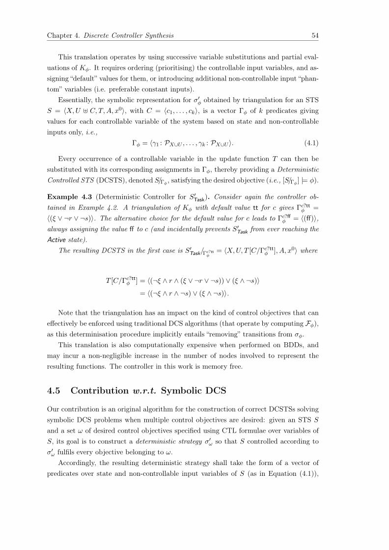
Chapter 4. Discrete Controller Synthesis 54
This translation operates by using successive variable substitutions and partial eval-uations of Kφ. It requires ordering (prioritising) the controllable input variables, and as-signing “default” values for them, or introducing additional non-controllable input “phan-tom” variables (i.e. preferable constant inputs).
Essentially, the symbolic representation for σ′φ obtained by triangulation for an STSS = 〈X,U ] C, T,A, x0〉, with C = 〈c1, . . . , ck〉, is a vector Γφ of k predicates givingvalues for each controllable variable of the system based on state and non-controllableinputs only, i.e.,
Γφ = 〈γ1 : PX∪U , . . . , γk : PX∪U 〉. (4.1)
Every occurrence of a controllable variable in the update function T can then besubstituted with its corresponding assignments in Γφ, thereby providing a DeterministicControlled STS (DCSTS), denoted S/Γφ , satisfying the desired objective (i.e., [S/Γφ ] |= φ).
Example 4.3 (Deterministic Controller for S′Task). Consider again the controller ob-tained in Example 4.2. A triangulation of Kφ with default value tt for c gives Γc?tt
φ =
〈(ξ ∨ ¬r ∨ ¬s)〉. The alternative choice for the default value for c leads to Γc?ffφ = 〈(ff)〉,
always assigning the value ff to c (and incidentally prevents S′Task from ever reaching theActive state).
The resulting DCSTS in the first case is S′Task/Γc?ttφ
= 〈X,U, T [C/Γc?ttφ ], A, x0〉 where
T [C/Γc?ttφ ] = 〈(¬ξ ∧ r ∧ (ξ ∨ ¬r ∨ ¬s)) ∨ (ξ ∧ ¬s)〉
= 〈(¬ξ ∧ r ∧ ¬s) ∨ (ξ ∧ ¬s)〉.
Note that the triangulation has an impact on the kind of control objectives that caneffectively be enforced using traditional DCS algorithms (that operate by computing Fφ),as this determinisation procedure implicitly entails “removing” transitions from σφ.
This translation is also computationally expensive when performed on BDDs, andmay incur a non-negligible increase in the number of nodes involved to represent theresulting functions. The controller in this work is memory free.
4.5 Contribution w.r.t. Symbolic DCS
Our contribution is an original algorithm for the construction of correct DCSTSs solvingsymbolic DCS problems when multiple control objectives are desired: given an STS Sand a set ω of desired control objectives specified using CTL formulae over variables ofS, its goal is to construct a deterministic strategy σ′ω so that S controlled according toσ′ω fulfils every objective belonging to ω.
Accordingly, the resulting deterministic strategy shall take the form of a vector ofpredicates over state and non-controllable input variables of S (as in Equation (4.1)),
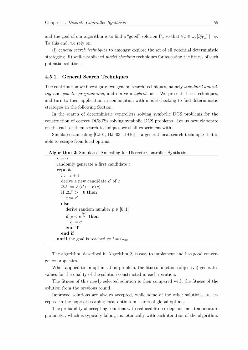
Chapter 4. Discrete Controller Synthesis 55
and the goal of our algorithm is to find a “good” solution Γω so that ∀φ ∈ ω, [S/Γω ] |= φ.To this end, we rely on:
(i) general search techniques to amongst explore the set of all potential deterministicstrategies; (ii) well-established model checking techniques for assessing the fitness of suchpotential solutions.
4.5.1 General Search Techniques
The contribution we investigate two general search techniques, namely simulated anneal-ing and genetic programming, and derive a hybrid one. We present these techniques,and turn to their application in combination with model checking to find deterministicstrategies in the following Section.
In the search of deterministic controllers solving symbolic DCS problems for theconstruction of correct DCSTSs solving symbolic DCS problems. Let us now elaborateon the each of them search techniques we shall experiment with.
Simulated annealing [CJ01, HJJ03, HS16] is a general local search technique that isable to escape from local optima.
Algorithm 2: Simulated Annealing for Discrete Controller Synthesisi := 0randomly generate a first candidate crepeati := i+ 1derive a new candidate c′ of c∆F := F (c′)− F (c)if ∆F >= 0 thenc := c′
elsederive random number p ∈ [0, 1]
if p < e∆Fθi then
c := c′
end ifend if
until the goal is reached or i = imax
The algorithm, described in Algorithm 2, is easy to implement and has good conver-gence properties.
When applied to an optimisation problem, the fitness function (objective) generatesvalues for the quality of the solution constructed in each iteration.
The fitness of this newly selected solution is then compared with the fitness of thesolution from the previous round.
Improved solutions are always accepted, while some of the other solutions are ac-cepted in the hope of escaping local optima in search of global optima.
The probability of accepting solutions with reduced fitness depends on a temperatureparameter, which is typically falling monotonically with each iteration of the algorithm.
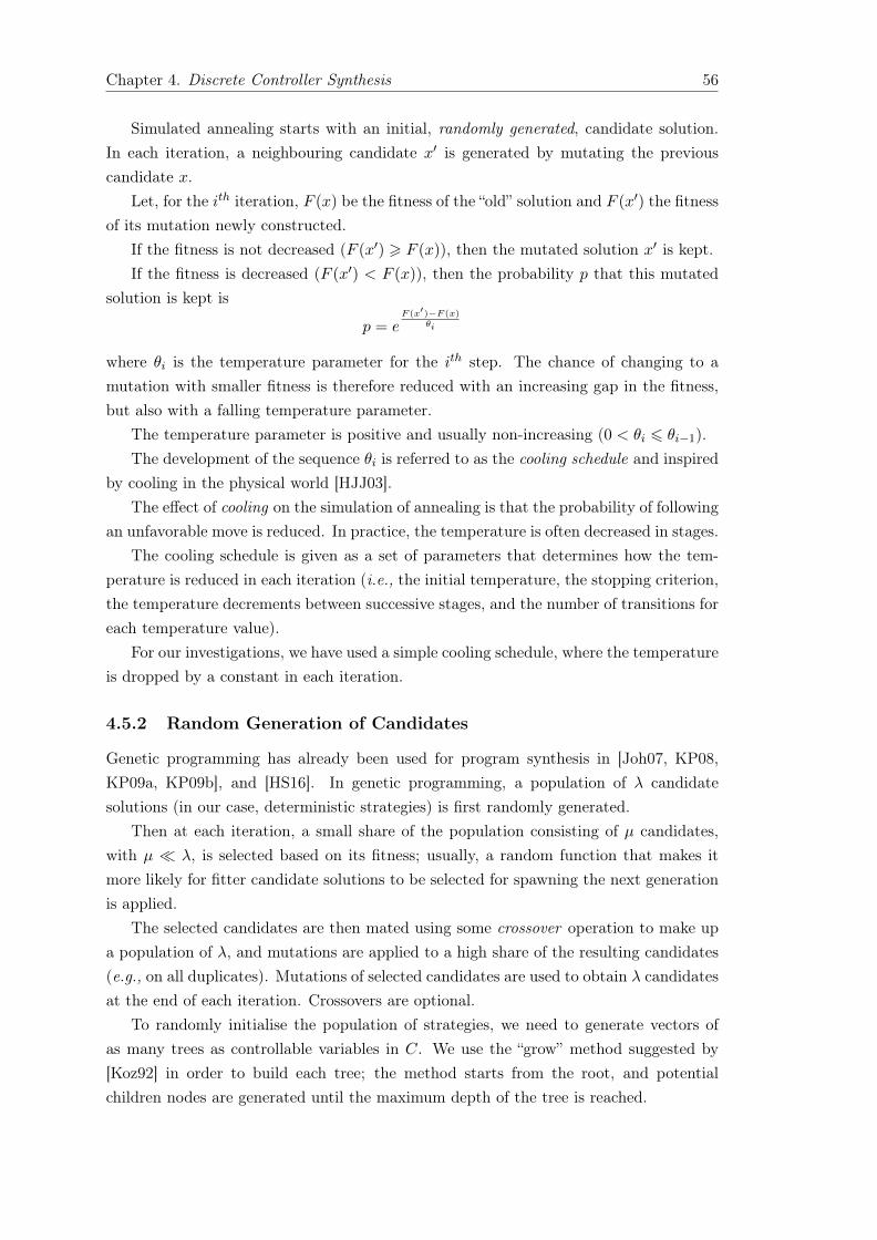
Chapter 4. Discrete Controller Synthesis 56
Simulated annealing starts with an initial, randomly generated, candidate solution.In each iteration, a neighbouring candidate x′ is generated by mutating the previouscandidate x.
Let, for the ith iteration, F (x) be the fitness of the “old” solution and F (x′) the fitnessof its mutation newly constructed.
If the fitness is not decreased (F (x′) > F (x)), then the mutated solution x′ is kept.If the fitness is decreased (F (x′) < F (x)), then the probability p that this mutated
solution is kept is
p = eF (x′)−F (x)
θi
where θi is the temperature parameter for the ith step. The chance of changing to amutation with smaller fitness is therefore reduced with an increasing gap in the fitness,but also with a falling temperature parameter.
The temperature parameter is positive and usually non-increasing (0 < θi 6 θi−1).The development of the sequence θi is referred to as the cooling schedule and inspired
by cooling in the physical world [HJJ03].The effect of cooling on the simulation of annealing is that the probability of following
an unfavorable move is reduced. In practice, the temperature is often decreased in stages.The cooling schedule is given as a set of parameters that determines how the tem-
perature is reduced in each iteration (i.e., the initial temperature, the stopping criterion,the temperature decrements between successive stages, and the number of transitions foreach temperature value).
For our investigations, we have used a simple cooling schedule, where the temperatureis dropped by a constant in each iteration.
4.5.2 Random Generation of Candidates
Genetic programming has already been used for program synthesis in [Joh07, KP08,KP09a, KP09b], and [HS16]. In genetic programming, a population of λ candidatesolutions (in our case, deterministic strategies) is first randomly generated.
Then at each iteration, a small share of the population consisting of µ candidates,with µ λ, is selected based on its fitness; usually, a random function that makes itmore likely for fitter candidate solutions to be selected for spawning the next generationis applied.
The selected candidates are then mated using some crossover operation to make upa population of λ, and mutations are applied to a high share of the resulting candidates(e.g., on all duplicates). Mutations of selected candidates are used to obtain λ candidatesat the end of each iteration. Crossovers are optional.
To randomly initialise the population of strategies, we need to generate vectors ofas many trees as controllable variables in C. We use the “grow” method suggested by[Koz92] in order to build each tree; the method starts from the root, and potentialchildren nodes are generated until the maximum depth of the tree is reached.

Chapter 4. Discrete Controller Synthesis 57
Algorithm 3: growmaxdepth (depth)
if depth < maxdepth thennode ← random (∨,∧,¬, tt,ff ∪X ∪ U)for each children child required for node do
node.child ← growmaxdepth (depth + 1)end for
elsenode ← random (tt,ff ∪X ∪ U)
end ifreturn node
growmaxdepth (depth) is shown as a recursive function in Algorithm 3, generating treesof maximum depth maxdepth. It takes the depth of the current node to be generated asargumentpredicate represented by the tree can be expressed. Initially depth=0.
If depth is less than the maximum tree depth, a node is chosen randomly from theset of terminals and binary operators. Then, depending on whether the node to generateis a terminal (leaf) or internal node, as many recursive calls as needed are performed tocreate the required number of children for the node.
If depth equals the maximum tree depth, then a node is chosen from the set ofterminals.
k) calls to grow1X∪U shall then be used to generate one candidate deterministicstrategy Γ.
Apart from simulated annealing and pure genetic programming with and withoutcrossovers as presented above, we additionally investigate a hybrid form introducing aproperty known from simulated annealing into the genetic programming algorithm: byappropriately tuning the measures of fitness, changes are applied more flexibly in thebeginning, while evolution becomes more rigid over time.
This hybrid approach has already been used for program synthesis in [KP08, KP09a?] as well as [HS16].
In our case, it basically consists in changing the candidate selection technique overtime, by first establishing the safety properties only, and then the liveness properties.
Just as for the genetic programming technique, crossovers are optional for this hybridapproach as well.
4.6 Principles of our DCS Algorithms
In this Section, we assume given an STS S = 〈X,U,C, T,A, x0〉 to be controlled, withC = 〈c1, . . . , ck〉, and a set of desired objective CTL formulae ω = φ1, . . . , φw.
4.6.1 Representing Deterministic Strategies
Recall that the candidate deterministic strategies are vectors of predicates involvingstate and non-controllable variables (cf. Section 4.5), and such candidates are subject to

Chapter 4. Discrete Controller Synthesis 58
mutations (and possibly crossovers) for genetic programming and simulated annealingalgorithms to be applicable. Therefore, one needs to find a suitable representation forsuch vectors of predicates.
Usual symbolic representations for predicates involve Binary Decision Diagrams (BDDs) [Bry86],for they yield good time and memory performance in practice. BDDs also enjoy an oftenuseful canonicity property, as every functionally equivalent predicates lead to a uniqueBDD.
Usual symbolic representations for predicates involve BDDs (cf. Section 4.3.3). Yet,implementing efficient random generation, mutations, and crossovers on such diagramsappears to be challenging, and more importantly, unnecessary w.r.t. the purpose of thischapter whose goal is only to perform a our goal of performing a preliminary feasibilityassessment for the use of general search techniques to solve symbolic DCS problems. Thecanonicity of candidates is not required by the algorithms we investigate either.
Therefore, we have opted for the simpler solution of using trees built according tothe grammar of predicates introduced in Section 4.3.1:
• each leaf is labelled with either a variable belonging to X ∪ U , or a constant intt,ff;
• each node with one children is labelled with ¬;
• each node with two children is labelled with a binary operator ∨ or ∧.
In the end, we represent candidate deterministic strategies as fixed-sized vectorsΓ = 〈γi〉i∈1,...,k of k trees γi as defined above, one per controllable variable in C.
Predicate consist of two parts, first a predicate P describes a relation or property,and variables (x, y) can take arbitrary values from some domain,P still have two truthvalues for statements (TandF ), When we assign values to x and y, then P has a truthvalue. This can be easily reprehend as a binary tree, in which mutations can be appliedin a simple way the using BDDs.
4.6.2 Performing Mutations and Crossovers
Mutations are changes applied on each candidate deterministic strategy Γ. Recall thatthe latter are represented as vectors of predicates involving state and non-controllablevariables (cf. Section 4.5). Such changes can be applied using a random walk on onetree of Γ as follows:
1. Randomly select a predicate γ to be changed in Γ;
2. Perform a random walk on γ from its root, randomly choosing to stop or visit one ofits children nodes (picked with uniform probability);
3. Perform a random walk on γ from its root, randomly choosing to stop or visit one ofits children nodes (picked with probabilities weighted by the number descendants);
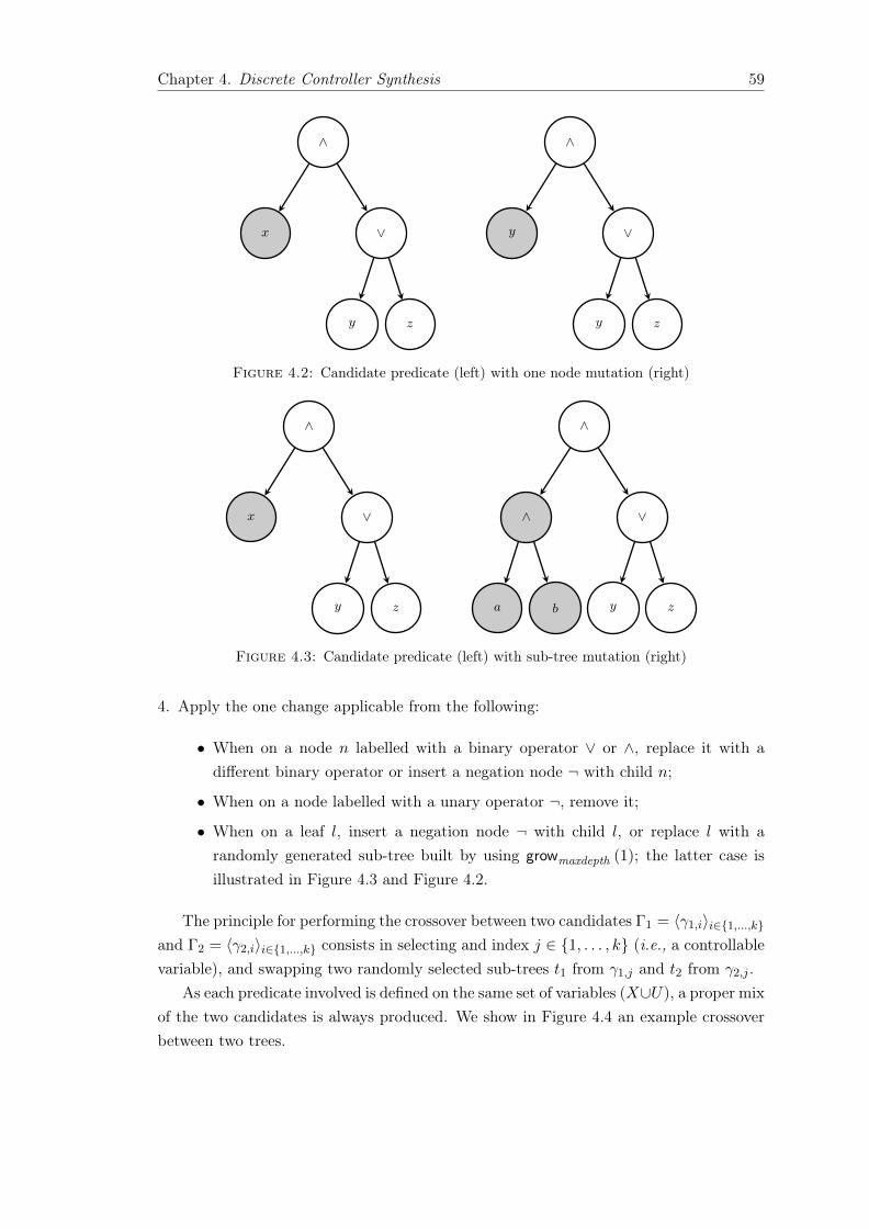
Chapter 4. Discrete Controller Synthesis 59
∧
x ∨
y z
∧
y ∨
y z
Figure 4.2: Candidate predicate (left) with one node mutation (right)
∧
x ∨
y z
∧
∧
a b
∨
y z
Figure 4.3: Candidate predicate (left) with sub-tree mutation (right)
4. Apply the one change applicable from the following:
• When on a node n labelled with a binary operator ∨ or ∧, replace it with adifferent binary operator or insert a negation node ¬ with child n;
• When on a node labelled with a unary operator ¬, remove it;
• When on a leaf l, insert a negation node ¬ with child l, or replace l with arandomly generated sub-tree built by using growmaxdepth (1); the latter case isillustrated in Figure 4.3 and Figure 4.2.
The principle for performing the crossover between two candidates Γ1 = 〈γ1,i〉i∈1,...,kand Γ2 = 〈γ2,i〉i∈1,...,k consists in selecting and index j ∈ 1, . . . , k (i.e., a controllablevariable), and swapping two randomly selected sub-trees t1 from γ1,j and t2 from γ2,j .
As each predicate involved is defined on the same set of variables (X∪U), a proper mixof the two candidates is always produced. We show in Figure 4.4 an example crossoverbetween two trees.

Chapter 4. Discrete Controller Synthesis 60
∧
∨
a b
∨
x y
∨
∧
c d
∧
y z
∧
∧
c d
∨
x y
∨
∨
a b
∧
y z
Figure 4.4: Crossover: two parents (above) and two offspring (below)
4.6.3 Model checking as a Fitness Function
We use model checking to determine the fitness of a candidate deterministic strategy ina way similar to that of [KP08, KP09a, KP09b] and [HS16] for program synthesis usinggenetic programming.
The model checking results are used to derive a quantitative measure for the fitness(as a level of partial correctness) of a deterministic strategy Γ w.r.t. the objectives ω.
To design a fitness measure for candidates, we make the hypothesis that the share ofobjectives that are satisfied so far by a candidate is a good indication of its pertinence.
We additionally observe that candidate solutions that satisfy weaker objectives—thatcan be mechanically derived from those belonging to ω—may be good candidates worthselecting for the generation of further potential solutions.For example, if a property shallhold on all paths (i.e., CTL formula of the form Aψ) , it is better if it holds on somepaths, and yet better if it holds almost surely.
Taking these observations into account, we first automatically translate the objectiveswith up to two universal path quantifiers occurring positively into weaker objectives:
• A first set of weaker objectives ω′ is obtained by selecting every objective from ω
featuring universal path quantifiers (i.e., Aψ), and replacing
Chapter 4. Discrete Controller Synthesis 61
• Repeating this process once again on eligible objectives of ω′ gives ω′′.
(We shall give example partial objectives as built by the above procedure in Sec-tion 4.7.1 below.)
Then, given a candidate deterministic strategy Γ and a set of objectives ω, a modelchecking algorithm is used to check whether [S/Γ] |= φ, for each objective φ in ω∪ω′∪ω′′
The fitness of Γ is computed based on the number of objectives of each set ω, ω′ andω′′ that it satisfies: m points are assigned per objective of ω that is satisfied, m′ points(with m′ < m) per objective of ω′, and m′′ points (with m′′ < m′) per objective of ω′′.
We offer an automated translation of properties with up to two universal quantifiersthat occur positively. 100 points are assigned when the sub-specification is satisfied, 80
points if the specification is satisfied when replacing one universal path quantifier by anexistential path quantifier, and 10 points are assigned if the specification is satisfied afterreplacing both universal path quantifiers by existential ones. (Existential quantifiers thatoccur negatively are treated accordingly.) Examples of this automated translation areshown in Chapter 3. Eventually, the main part of the fitness is the average of the valuesfor all considered objectives ω in the rigid evaluation, and the average of all livenessobjectives ωl in the flexible evaluation.
Following the works of [KP08] and [HS16], we also apply a penalty for “large” strate-gies by deducing the number of inner nodes of all trees from this average when assigningthe fitness of a candidate strategy.
Let us denote Fω (Γ) the fitness value obtained as described above for the candidateΓ and objectives ω.
4.6.4 Variants for Improved Search Techniques
To derive improved variants of the general search algorithms of Section 4.5.1, we notethat a subset ωs of given target objectives ω are safety ones, while the others ωl (= ω\ωs)are considered liveness objectives1.
At each iteration of the simulated annealing algorithm, the first decision to select anew candidate Γ′ over an old one Γ (condition ∆F < 0 in Algorithm 2) is taken accordingto one of two distinct policies, giving two versions of the simulated annealing algorithm:
rigid Γ′ is selected at this stage whenever Fω (Γ′) > Fω (Γ);
flexible Γ′ is selected at this stage whenever Fω (Γ′) > Fω (Γ) or Fωs (Γ′) > Fωs (Γ); Γ′
is always discarded when Fωs (Γ′) < Fωs (Γ).
The resulting fitness value will be used by simulated annealing to compare the currentcandidate with the previous one when using rigid evaluation, and to make a decisionwhether the changes will be preserved or discarded.
1One can use a simple syntactical criterion for deciding that an objective surely belongs to ωs; e.g.,some safety CTL formulae can be rewritten as AGϕ with ϕ ∈ PX .
Chapter 4. Discrete Controller Synthesis 62
When using flexible evaluation, this only happens if the value for the safety spec-ification is equal; falling (resp. rising) values for safety specifications always result indiscarding (resp. selecting) the update when using flexible evaluation.
Our implementation of the hybrid algorithm presented in Chapter 2 basically consistsin tuning the evaluation of fitness to first favour safety objectives: in this algorithm,the fitness Fω (Γ) of a candidate Γ is actually made of the pair (Fωs (Γ) , Fωl (Γ)), andcomparisons of such fitness measures are performed according to their lexical ordering.
This way, candidates with better values for the safety objectives ωs are always givenpreference, while the fitness computed using liveness objectives ωl only are merely tie-breakers for equal values of Fωs (Γ).
selection technique over time. It first evaluates the fitness of each candidate Γ usingsafety objectives only (Fωs (Γ)). Then, over a second phase, it continues by taking allobjectives ω into account to measure the fitness (Fω (Γ)).
properties, and then the liveness properties. Specifications with better values for thesafety properties are always given preference, while liveness properties are—for equalvalues for the safety properties—used to determine the fitness. i.e., they are merelytie-breakers.
This approach has been used in [HS16] as well as [KP08, KP09a, KP09b]. We referto it as a hybrid approach as it introduces a property known from simulated annealing:in the beginning, the algorithm is applying changes more flexibly, while it becomes morerigid later.
crossover, and used both evaluation techniques for simulated annealing, where werefer to using the classic fitness function as a rigid evaluation, and to the hybrid approachas flexible evaluation.
In the end, we investigate and compare six algorithms involving various search tech-niques:
1. pure genetic programming without crossovers (GP); and2. with crossovers (GP w. CO);3. rigid simulated annealing (SA rigid);4. flexible simulated annealing (SA flexible);5. hybrid search without crossovers (Hybrid); and6. with crossovers (Hybrid w. CO).
4.7 Experimental Feasibility Assessment
4.7.1 Problem Instances
In order to get a preliminary feasibility assessment of our approach, we have generatedseveral problem instances based on the parallel composition of STSs as per Remark 4.2.Synthesis objectives were then derived as CTL formulae in a scalable manner.
Regarding the STSs, each problem N–Tasks was built using composition of N in-stances of the STS S′Task described in Example 4.2 (modulo renaming of variables to

Chapter 4. Discrete Controller Synthesis 63
ensure disjointness); i.e., the STSs involved were built as
SN–Tasks =∥∥i∈1,...,N〈Xi, Ui ] Ci, Ti, Ai, x0
i 〉,
where Xi = 〈ξi〉, U = 〈ri, si〉, Ci = 〈ci〉, Ti = 〈(¬ξi ∧ ri ∧ ci) ∨ (ξi ∧ si)〉, Ai = tt, andx0i = ξi 7→ ff.Objective CTL formulae for each problem N–Tasks consist of both safety ωs,N and
liveness ωl,N objectives.Regarding safety, mutual exclusion properties suit our need for scalable, CTL formu-
lae that are relatively complex to represent: i.e., no two tasks should be in their Activestate (with ξi = tt) at the same time.
For each problem instance N–Tasks, one obtains:
ωs,N =
AG ∧i∈1,...,N−1
∧j∈i+1,...,N
¬ (ξi ∧ ξj)
,
with notable special case ωs,1 = ∅. As a concrete illustration, one obtains ωs,2 =
AG(¬(ξ1 ∧ ξ2)).Regarding liveness objectives ωl,N , we want to ensure that every task in its Idle state
should eventually reach its Active state. Formally, one obtains:
ωl,N =⋃
i∈1,...,N
AG (¬ξi ⇒ AFξi).
AG(¬ξ1 ⇒ AFξ1)
AG(¬ξ2 ⇒ AFξ2)
Those two are the liveness properties (any task on idle state will definitely be on theactive state in the future)
In the end, solving each problem N–Tasks consists in finding a deterministic strategyΓωN so that ∀φ ∈ ωN , [SN–Tasks/ΓωN ] |= φ, with ωN = ωs,N ∪ ωl,N .
Partial Objectives The partial objectives automatically generated from the ωs,N ’sand ωl,N ’s above, according to the procedure explained in Section 4.6.3, are:
ω′s,N =
EG ∧i∈1,...,N−1
∧j∈i+1,...,N
¬ (ξi ∧ ξj)
,
and ω′′s,N = ∅.Informally, partial objectives in ω′s,N state that there exists execution paths where
the mutual exclusion property is met.On the other hand, the ωl,N ’s lead to:
Chapter 4. Discrete Controller Synthesis 64
ω′l,N =⋃
i∈1,...,N
AG (¬ξi ⇒ EFξi) , EG (¬ξi ⇒ AFξi),
andω′′l,N =
⋃i∈1,...,N
EG (¬ξi ⇒ EFξi).
4.7.2 Experimental Setup
We have implemented the simulated annealing, and genetic programming, and hybridalgorithms as described, using NuSMV [CCG+02] as a solver to derive the fitness ofcandidate deterministic strategies.
For simulated annealing, we have set the initial temperature to 20,000. The coolingschedule decreases the temperature by 0.8 in each iteration. Thus, the schedule endsafter 25,000 iterations, when the temperature hits 0. In a failed execution, this leads todetermining the fitness of 25,001 candidates.
We have taken the values suggested in [KP08] and [HS16] for genetic programming:λ = 150 candidates are considered in each step, µ = 5 are kept, and we abort after2,000 iterations. In a failed execution, this leads to determining the fitness of 290,150candidates.
Points assigned for fitness measures are arbitrarily set to m = 100 for target objec-tives, and m′ = 80 and m′′ = 10 for partial objectives Those evaluation numbers aregiven to weight the candidates and distinguish among three levels of them according tothe satisfaction of the specifications. This means that it is possible to take another values(eg. 20, 60, and 100) the most important thing is keep the difference among them clear(cf. Section 4.6.3).
The experiments have been conducted using a machine with an Intel core i7 3.40GHz CPU and 16GB RAM.
4.7.3 Experimental Results
2The results are shown in Figures 4.5 and 4.7 and summarised in Table 4.1. Figure 4.5shows the average time needed for synthesising a correct candidates.
The two factors that determine the average running time are the success rate andthe running time for a full execution, successful or not.
These values are shown in Figure 4.7. Table 4.1 shows the average running time forsingle executions in seconds, the success rate in %, and the resulting overall runningtime.
2In all tables, execution times are in seconds; t is the mean execution time of single executions(succeeding or failing), and columns “expec. time” extrapolate t based on the success rate obtained in100 single executions (“suc. %”).

Chapter 4. Discrete Controller Synthesis 65
SA rigid SA flexible Hybrid Hybrid w. CO GP GP w. CO0
5,000
10,000
15,000
20,000
25,000
30,000
35,000
40,000
45,000
50,000Overalltimein
second
s1–Task2–Tasks3–Tasks4–Tasks5–Tasks6–Tasks
Figure 4.5: Overall time required for synthesising a correct candidate
SA rigid SA flexible Hybrid Hybrid w. CO GP GP w. CO0
200
400
600
800
1,000
Individu
alexecutiontimein
second
s
1–Task2–Tasks3–Tasks4–Tasks5–Tasks6–Tasks
Figure 4.6: Average running time of an individual execution

Chapter 4. Discrete Controller Synthesis 66
SA rigid SA flexible Hybrid Hybrid w. CO GP GP w. CO0
2
4
6
8
10
12
14
16
18
20
22Su
ccessrate
1–Task2–Tasks3–Tasks4–Tasks5–Tasks6–Tasks
Figure 4.7: Success rate of individual executions
The best values (shortest expected running time or highest success rate) for eachcomparison printed in bold. Both simulated annealing and the hybrid approach signif-icantly outperform the pure genetic programming approach. The low success rate forpure genetic programming suggests that the number of iterations might be too small.
However, as the individual execution time is already ways above the average timesimulated annealing needs for constructing a correct candidate, we did not increase thenumber of iterations.
The advantage in the individual execution time between the classic and the hybridversion of genetic programming is in the range that is to be expected, as the number ofcalls to the model-checker is reduced. It is interesting to note that simulated annealing,where the shift from rigid to flexible evaluation might be expected to have a similareffect, does not benefit to the same extent.
It is also interesting to note that the execution time suggests that determining thefitness of candidates produced by simulated annealing is slightly more expensive. Thiswas to be expected, as the average candidate size grows over time.
The penalty for longer candidates reduces this effect, but cannot entirely remove it.(This potential disadvantage is the reason why an occasional re-start provides betterresults than prolonging the search.)
As was the case in our previous work [HS16], it is interesting to note that both thepure and the hybrid approach to genetic programming benefit from crossovers.
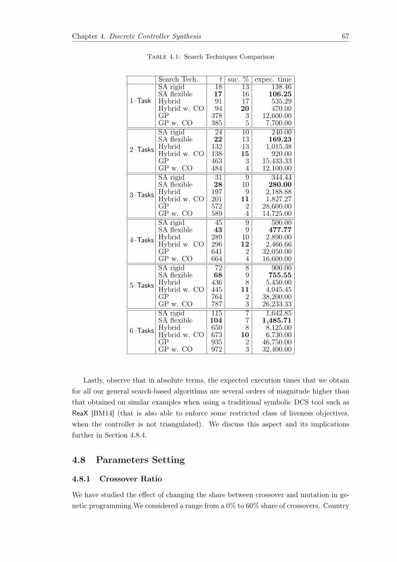
Chapter 4. Discrete Controller Synthesis 67
Table 4.1: Search Techniques Comparison
Search Tech. t suc. % expec. time
1–Task
SA rigid 18 13 138.46SA flexible 17 16 106.25Hybrid 91 17 535.29Hybrid w. CO 94 20 470.00GP 378 3 12,600.00GP w. CO 385 5 7,700.00
2–Tasks
SA rigid 24 10 240.00SA flexible 22 13 169.23Hybrid 132 13 1,015.38Hybrid w. CO 138 15 920.00GP 463 3 15,433.33GP w. CO 484 4 12,100.00
3–Tasks
SA rigid 31 9 344.44SA flexible 28 10 280.00Hybrid 197 9 2,188.88Hybrid w. CO 201 11 1,827.27GP 572 2 28,600.00GP w. CO 589 4 14,725.00
4–Tasks
SA rigid 45 9 500.00SA flexible 43 9 477.77Hybrid 289 10 2,890.00Hybrid w. CO 296 12 2,466.66GP 641 2 32,050.00GP w. CO 664 4 16,600.00
5–Tasks
SA rigid 72 8 900.00SA flexible 68 9 755.55Hybrid 436 8 5,450.00Hybrid w. CO 445 11 4,045.45GP 764 2 38,200.00GP w. CO 787 3 26,233.33
6–Tasks
SA rigid 115 7 1,642.85SA flexible 104 7 1,485.71Hybrid 650 8 8,125.00Hybrid w. CO 673 10 6,730.00GP 935 2 46,750.00GP w. CO 972 3 32,400.00
Lastly, observe that in absolute terms, the expected execution times that we obtainfor all our general search-based algorithms are several orders of magnitude higher thanthat obtained on similar examples when using a traditional symbolic DCS tool such asReaX [BM14] (that is also able to enforce some restricted class of liveness objectives,when the controller is not triangulated). We discuss this aspect and its implicationsfurther in Section 4.8.4.
4.8 Parameters Setting
4.8.1 Crossover Ratio
We have studied the effect of changing the share between crossover and mutation in ge-netic programming.We considered a range from a 0% to 60% share of crossovers. Country

Chapter 4. Discrete Controller Synthesis 68
to our expectation, we did not observe any relevant effect of in- or decreasing the shareof cross over for either classic or hybrid genetic programming. Interestingly, the run-ning time per instance increased with the share of crossovers, which might point to aproduction of more complex programs. See Tables 4.2 and 4.3.
ratio % t suc. % expec. time
1 Task0 378 4 945020 385 5 770040 403 5 806060 418 4 1045080 425 3 14166.67100 438 1 43800
2 Tasks0 475 3 15833.3320 484 4 1210040 491 4 1227560 501 3 1670080 509 2 25450100 521 1 52100
3 Tasks0 571 3 19033.3320 589 4 1472540 597 3 1990060 606 3 2020080 613 1 61300100 627 1 62700
4 Tasks0 658 3 21933.3320 664 4 1660040 679 4 1697560 687 3 2290080 693 2 34650100 711 1 71100
5 Tasks0 776 1 7760020 787 3 26233.3340 792 3 2640060 799 2 3995080 804 2 40200100 815 1 81500
6 Tasks0 961 2 4805020 972 3 3240040 981 2 4905060 989 2 4945080 997 2 49850100 1011 1 101100
Table 4.2: Crossover ratio for GP (Discrete Controller Synthesis)
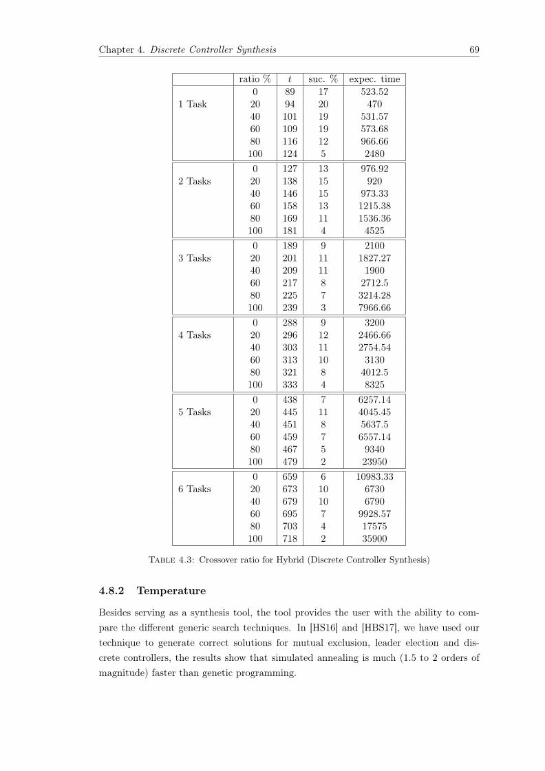
Chapter 4. Discrete Controller Synthesis 69
ratio % t suc. % expec. time
1 Task0 89 17 523.5220 94 20 47040 101 19 531.5760 109 19 573.6880 116 12 966.66100 124 5 2480
2 Tasks0 127 13 976.9220 138 15 92040 146 15 973.3360 158 13 1215.3880 169 11 1536.36100 181 4 4525
3 Tasks0 189 9 210020 201 11 1827.2740 209 11 190060 217 8 2712.580 225 7 3214.28100 239 3 7966.66
4 Tasks0 288 9 320020 296 12 2466.6640 303 11 2754.5460 313 10 313080 321 8 4012.5100 333 4 8325
5 Tasks0 438 7 6257.1420 445 11 4045.4540 451 8 5637.560 459 7 6557.1480 467 5 9340100 479 2 23950
6 Tasks0 659 6 10983.3320 673 10 673040 679 10 679060 695 7 9928.5780 703 4 17575100 718 2 35900
Table 4.3: Crossover ratio for Hybrid (Discrete Controller Synthesis)
4.8.2 Temperature
Besides serving as a synthesis tool, the tool provides the user with the ability to com-pare the different generic search techniques. In [HS16] and [HBS17], we have used ourtechnique to generate correct solutions for mutual exclusion, leader election and dis-crete controllers, the results show that simulated annealing is much (1.5 to 2 orders ofmagnitude) faster than genetic programming.
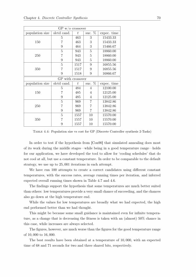
Chapter 4. Discrete Controller Synthesis 70
GP w/o crossoverpopulation size slctd cand. t suc. % expec. time
1505 463 3 15433.337 463 3 15433.339 464 3 15466.67
2505 943 5 18860.007 943 5 18860.009 943 5 18860.00
3505 1517 9 16855.567 1517 9 16855.569 1518 9 16866.67
GP with crossoverpopulation size slctd cand. t suc. % expec. time
1505 484 4 12100.007 485 4 12125.009 485 4 12125.00
2505 969 7 13842.867 969 7 13842.869 969 7 13842.86
3505 1557 10 15570.007 1557 10 15570.009 1557 10 15570.00
Table 4.4: Population size vs cost for GP (Discrete Controller synthesis 2-Tasks)
In order to test if the hypothesis from [Con90] that simulated annealing does mostof its work during the middle stages—while being in a good temperature range—holdsfor our application, we have developed the tool to allow for ‘cooling schedules’ that donot cool at all, but use a constant temperature. In order to be comparable to the defaultstrategy, we use up to 25, 001 iterations in each attempt.
We have run 100 attempts to create a correct candidates using different constanttemperatures, with the success rates, average running times per iteration, and inferredexpected overall running times shown in Table 4.7 and 4.6.
The findings support the hypothesis that some temperatures are much better suitedthan others: low temperatures provide a very small chance of succeeding, and the chancesalso go down at the high temperature end.
While the values for low temperatures are broadly what we had expected, the highend performed better than we had thought.
This might be because some small guidance is maintained even for infinite tempera-ture, as a change that is decreasing the fitness is taken with an (almost) 50% chance inthis case, while increases are always selected.
The figures, however, are much worse than the figures for the good temperature rangeof 10, 000 to 16, 000.
The best results have been obtained at a temperature of 10, 000, with an expectedtime of 68 and 71 seconds for two and three shared bits, respectively.
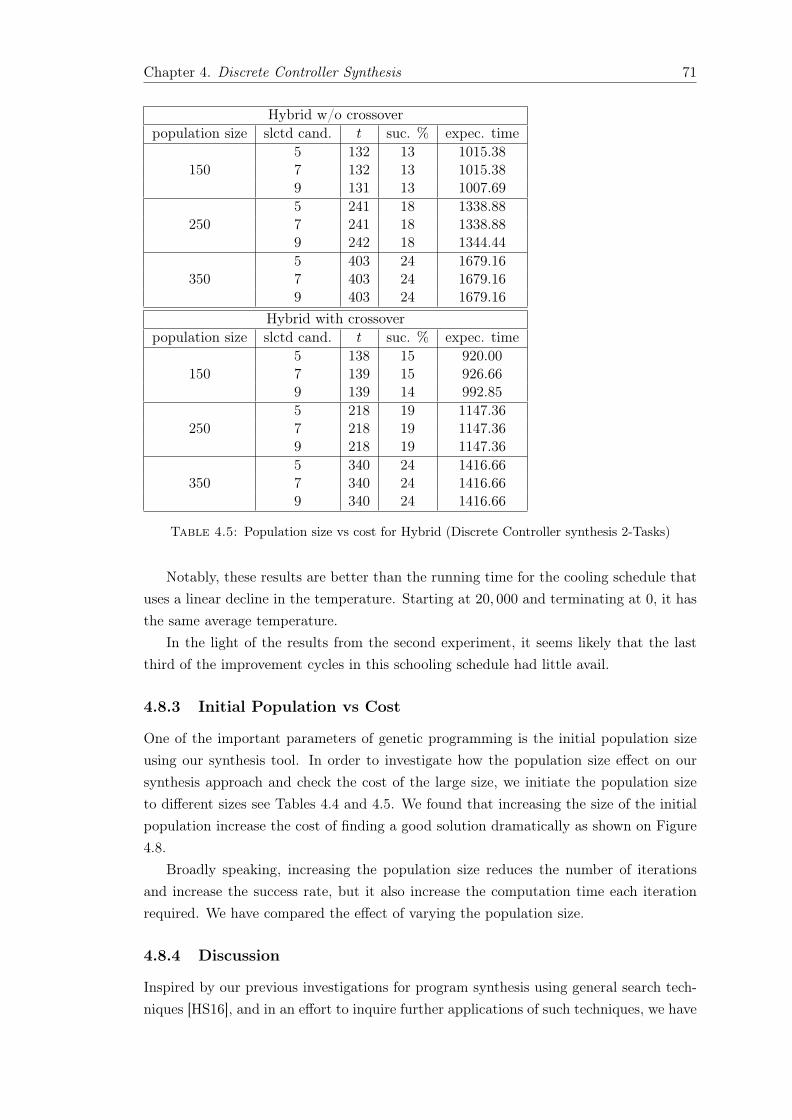
Chapter 4. Discrete Controller Synthesis 71
Hybrid w/o crossoverpopulation size slctd cand. t suc. % expec. time
1505 132 13 1015.387 132 13 1015.389 131 13 1007.69
2505 241 18 1338.887 241 18 1338.889 242 18 1344.44
3505 403 24 1679.167 403 24 1679.169 403 24 1679.16
Hybrid with crossoverpopulation size slctd cand. t suc. % expec. time
1505 138 15 920.007 139 15 926.669 139 14 992.85
2505 218 19 1147.367 218 19 1147.369 218 19 1147.36
3505 340 24 1416.667 340 24 1416.669 340 24 1416.66
Table 4.5: Population size vs cost for Hybrid (Discrete Controller synthesis 2-Tasks)
Notably, these results are better than the running time for the cooling schedule thatuses a linear decline in the temperature. Starting at 20, 000 and terminating at 0, it hasthe same average temperature.
In the light of the results from the second experiment, it seems likely that the lastthird of the improvement cycles in this schooling schedule had little avail.
4.8.3 Initial Population vs Cost
One of the important parameters of genetic programming is the initial population sizeusing our synthesis tool. In order to investigate how the population size effect on oursynthesis approach and check the cost of the large size, we initiate the population sizeto different sizes see Tables 4.4 and 4.5. We found that increasing the size of the initialpopulation increase the cost of finding a good solution dramatically as shown on Figure4.8.
Broadly speaking, increasing the population size reduces the number of iterationsand increase the success rate, but it also increase the computation time each iterationrequired. We have compared the effect of varying the population size.
4.8.4 Discussion
Inspired by our previous investigations for program synthesis using general search tech-niques [HS16], and in an effort to inquire further applications of such techniques, we have
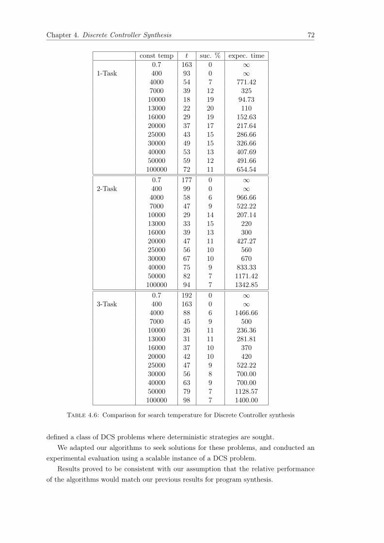
Chapter 4. Discrete Controller Synthesis 72
const temp t suc. % expec. time
1-Task0.7 163 0 ∞400 93 0 ∞4000 54 7 771.427000 39 12 32510000 18 19 94.7313000 22 20 11016000 29 19 152.6320000 37 17 217.6425000 43 15 286.6630000 49 15 326.6640000 53 13 407.6950000 59 12 491.66100000 72 11 654.54
2-Task0.7 177 0 ∞400 99 0 ∞4000 58 6 966.667000 47 9 522.2210000 29 14 207.1413000 33 15 22016000 39 13 30020000 47 11 427.2725000 56 10 56030000 67 10 67040000 75 9 833.3350000 82 7 1171.42100000 94 7 1342.85
3-Task0.7 192 0 ∞400 163 0 ∞4000 88 6 1466.667000 45 9 50010000 26 11 236.3613000 31 11 281.8116000 37 10 37020000 42 10 42025000 47 9 522.2230000 56 8 700.0040000 63 9 700.0050000 79 7 1128.57100000 98 7 1400.00
Table 4.6: Comparison for search temperature for Discrete Controller synthesis
defined a class of DCS problems where deterministic strategies are sought.We adapted our algorithms to seek solutions for these problems, and conducted an
experimental evaluation using a scalable instance of a DCS problem.Results proved to be consistent with our assumption that the relative performance
of the algorithms would match our previous results for program synthesis.

Chapter 4. Discrete Controller Synthesis 73
const temp t suc. % expec. time
4-Task0.7 332 0 ∞400 167 0 ∞4000 98 3 3266.667000 65 6 1083.3310000 39 9 433.3313000 43 11 390.9016000 58 9 644.4420000 67 9 744.4425000 81 7 1157.1430000 89 6 1483.3340000 95 6 1583.3350000 103 5 2060100000 118 4 2950
5-Task0.7 298 0 ∞400 153 0 ∞4000 98 4 24507000 79 6 1316.6610000 61 9 677.7713000 67 10 67016000 73 8 912.520000 81 6 135025000 89 6 1483.3330000 102 4 255040000 116 3 3866.6650000 128 4 3200100000 178 3 5933.33
6-Task0.7 613 0 ∞400 598 0 ∞4000 278 3 9266.667000 125 5 250010000 99 8 1237.513000 115 9 1277.7716000 127 9 1411.1120000 134 7 1914.2825000 152 6 2533.3330000 159 6 265040000 168 6 280050000 192 5 3840100000 253 6325
Table 4.7: Comparison for search temperature for Discrete Controller
As noted in Section 4.7, our experimental results do not compare favourably withexisting symbolic DCS tools.
Yet, our implementations are proofs of concept, and one can think of numerouspractical improvements that constitute inescapable ways to pursue investigating efficientsymbolic DCS algorithms using simulated annealing
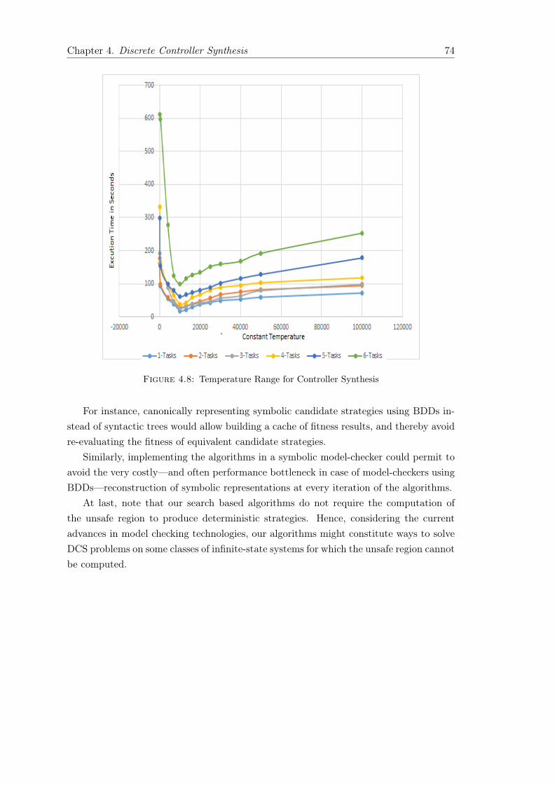
Chapter 4. Discrete Controller Synthesis 74
Figure 4.8: Temperature Range for Controller Synthesis
For instance, canonically representing symbolic candidate strategies using BDDs in-stead of syntactic trees would allow building a cache of fitness results, and thereby avoidre-evaluating the fitness of equivalent candidate strategies.
Similarly, implementing the algorithms in a symbolic model-checker could permit toavoid the very costly—and often performance bottleneck in case of model-checkers usingBDDs—reconstruction of symbolic representations at every iteration of the algorithms.
At last, note that our search based algorithms do not require the computation ofthe unsafe region to produce deterministic strategies. Hence, considering the currentadvances in model checking technologies, our algorithms might constitute ways to solveDCS problems on some classes of infinite-state systems for which the unsafe region cannotbe computed.

Chapter 4. Discrete Controller Synthesis 75
Figure 4.9: Initial Population Size vs Cost for Discrete Controller synthesis


Chapter 5
Complexity
5.1 Introduction
Discrete Controller Synthesis (DCS) and Program Synthesis have a similar theoreticalbackground: they are produce a control strategy and an implementation automatically,and also correct by construction.
The main differences between these two classes of problems, that DCS typicallyoperates on the model of a plant. It seeks the automated construction of a strategy tocontrol the plant, such that its runs satisfy a set of given objectives [RW89, AMP95].
Similarly, program synthesis seeks to infer an implementation, often of a reactivesystem, such that the runs of this system satisfy a given specification. While the mainargument supporting this technique is practical, it is interesting to consider the com-plexity of this approach, too. For the estimation of the complexity, we look at recurrentapplication of simulated annealing, as, from the figures from the previous Section, thisseems to be the most promising approach.
Also, applying the procedure repeatedly is fairly normal, as not 100% of the attemptslead to a deterministic strategy that satisfies all required objectives.
For our complexity consideration, we consider cooling schedules that change slowly.The reason for this is that the search space for a given cooling schedule is finite,
as only a finite set of deterministic strategies can be constructed with a fixed coolingschedule.
We naturally can only refer to probabilistic complexity here:it is always possible to only consider two neighbouring candidate strategies during all
runs (this is the case when candidate two is always selected as a mutation of candidateone and, vice versa, candidate one is always chosen as a mutation of candidate two),even when re-starting infinitely often.
This chapter provides a summary of the complexity analysis of the approach used inthis thesis. The rest of this section is organised as follows:
5.2.1 presents the complexity analysis of the program synthesis approach. Section5.2.2 provides a summary he complexity analysis of the discrete controller synthesisapproach.
77
Chapter 5. Complexity 78
5.2 Complexity Analysis
5.2.1 Program Synthesis
Theorem 5.1. Let s be the length of the specification and m the minimal size of thecorrect program. We show that there is a recurrent cooling schedule such that, with veryhigh probability,
• the space required is the space required for model checking programs of length O(m)
against specifications of length s and
• the time requirement is mO(m) times the time required for model checking programsof length O(m) against specifications of length s.
With very high probability means that, for all p < 1, one gets a result with probabilitygreater than p in the mentioned time and space class. Note that this refers to the samecooling schedule.
As a preparation for the proof of Theorem 5.2, we estimate the chance of producinga correct program in exactly m steps by a particular derivation of the program tree. Thechance is the product of the m transitions being made.
An individual transition can be described as the product of the chance that it isselected by the mutation algorithm and the chance that the algorithm continues withthe mutated form.
The chance of selecting a particular position for the mutation is Ω1i in the ith step,
and the chance of attempting a particular mutation when this position is selected is aconstant. (For the argument, it suffices that it is at least 1
O(poly(m)) .)If the chance is bounded from below by a constant – or even by a polynomial1
O(poly(m)) , then the chance is bounded from below by 1O(m)! .
For a given number n of steps (e.g., n = m if we have an oracle that tells us the sizeof the program we are looking for), it is easy to construct a cooling schedule with thisproperty: any cooling schedule that keeps the temperature sufficiently high for at leastn steps.
To avoid an unduly high time or space consumption of one iteration, the coolingafter this should proceed quickly, such that the overall number of mutation attemptsconsidered, nattempts, is in O(n).
As we would normally not know a suitable n ≥ m, we suggest to adjust the coolingschedule over time by increasing it slowly: in the ith iteration, we could use, for someconstant c ∈ N, the cooling scheme for ni = c + maxk ∈ N | k! ≤ i. Let us choosec = 0 for the proof.
of Theorem 5.1. For ni < m, we estimate the chance of creating a correct program with0. Note that nm! ≥ m. The time and space consumption of each of these steps can beestimated by the cost of model checking a program of size mattempts ∈ O(m) against aspecification of size s. There are less than m! of these attempts.
Chapter 5. Complexity 79
For ni ≥ m, the chance of creating a correct program is at least 1O(m)! . To create
a program with an arbitrary (but fixed) chance of at least p ∈ [0, 1[ therefore requiresO(m)! such steps.
The time and space consumption of each these steps can be estimated by the cost ofmodel checking a program of size O(m) against a specification of size s.
Note that this technique does not qualify as a decision procedure, as it cannot providea negative answer. (What it can be used to provide is an answer that, for a given m ∈ Nand p ∈ [0, 1[ there is no program of size at most m with a chance of at least p.)
Note further that the proof does not refer to a particular specification language. Forspace requirements, the complexity is, for relevant languages like LTL or CTL, as goodas one can hope.
With regard to time complexity, the complexity of synthesis is exponential for CTLand doubly exponential for LTL. If the expected time complexity of this algorithm ishigher depends on the question of whether or not PSPACE equals EXPTIME [FPS15].
5.2.2 Discrete Controller Synthesis
For the estimation of the complexity, we look at recurrent application of simulated anneal-ing, as, from the figures from the previous Section, this seems to be the most promisingapproach.
Also, applying the procedure repeatedly is fairly normal, as not 100% of the attemptslead to a deterministic strategy that satisfies all required objectives.
For our complexity consideration, we consider cooling schedules that change slowly.The reason for this is that the search space for a given cooling schedule is finite,
as only a finite set of deterministic strategies can be constructed with a fixed coolingschedule.
We naturally can only refer to probabilistic complexity here:it is always possible to only consider two neighbouring candidate strategies during all
runs (this is the case when candidate two is always selected as a mutation of candidateone and, vice versa, candidate one is always chosen as a mutation of candidate two),even when re-starting infinitely often.
Theorem 5.2. Let s be the length of the specification (some of the lengths of the targetobjectives in ω) and m the minimal size of the correct deterministic strategy. We showthat there is a recurrent cooling schedule such that, with very high probability,
• the space required is the space required for model-checking STSs of length O(m)
against specifications of length s and
• the time requirement is mO(m) times the time required for model-checking STSs oflength O(m) against specifications of length s.

Chapter 5. Complexity 80
With very high probability means that, for all p < 1, one gets a result with probabilitygreater than p in the mentioned time and space class. Note that this refers to the samecooling schedule.
As a preparation for the proof of Theorem 5.2, we estimate the chance of producinga correct strategy in exactly m steps by a particular derivation of the correspondingpredicate trees. The chance is the product of the m transitions being made.
An individual transition can be described as the product of the chance that it isselected by the mutation algorithm and the chance that the algorithm continues withthe mutated form.
The chance of selecting a particular position for the mutation is Ω(
1i
)in the ith step—
this lower bound stems from taking the weight of subtrees into account in the randomwalk, which can be used to select all nodes with equal probability—and the chance ofattempting a particular mutation when this position is selected is a constant.
(For the argument, it suffices that it is at least 1O(poly(m)) .) If the chance is bounded
from below by a constant – or even by a polynomial 1O(poly(m)) , then the chance is bounded
from below by 1O(m)! .
For a given number n of steps (e.g., n = m if we have an oracle that tells us the sizeof the predicate trees we are looking for), it is easy to construct a cooling schedule withthis property: any cooling schedule that keeps the temperature sufficiently high for atleast n steps.
To avoid an unduly high time or space consumption of one iteration, the coolingafter this should proceed quickly, such that the overall number of mutation attemptsconsidered, nattempts, is in O(n).
As we would normally not know a suitable n ≥ m, we suggest to adjust the coolingschedule over time by increasing it slowly: in the ith iteration, we could use, for someconstant c ∈ N, the cooling scheme for ni = c + maxk ∈ N | k! ≤ i. Let us choosec = 0 for the proof.
Proof of Theorem 5.2. For ni < m, we estimate the chance of creating a correct strategywith 0. Note that nm! ≥ m.
The time and space consumption of each of these steps can be estimated by the costof model-checking a strategy represented by predicate trees of size mattempts ∈ O(m)
against a specification of size s.There are less than m! of these attempts.For ni ≥ m, the chance of creating a correct strategy is at least 1
O(m)! .To create a strategy with an arbitrary (but fixed) chance of at least p ∈ [0, 1] therefore
requires O(m)! such steps. The time and space consumption of each of these steps canbe estimated by the cost of model-checking a strategy represented by predicate trees ofsize O(m) against a specification of size s.

Chapter 5. Complexity 81
Note that this technique does not qualify as a decision procedure, as it cannot providea negative answer. (What it can be used to provide is an answer that, for a given m ∈ Nand p ∈ [0, 1[ there is no strategy of size at most m with a chance of at least p.)
Note further that the proof does not refer to a particular specification language.For space requirements, the complexity is, for relevant languages like LTL or CTL,
as good as one can hope.With regard to time complexity, the complexity of synthesis is exponential for CTL
and doubly exponential for LTL.If the expected time complexity of this algorithm is higher depends on the question
of whether or not PSPACE equals EXPTIME [FPS15].

Chapter 6
Implementation
6.1 Abstract
PranCS [HSB17] is a tool for protocol and control synthesis. It is based on exploitinggeneral search techniques, simulated annealing and genetic programming, that use modelchecking for the fitness function. Based on this fitness, simulated annealing and geneticprogramming is used as a general search technique for homing in on an implementation.We use NuSMV as a back-end for the individual model checking tasks and a simplecandidate mutator to drive the search.
Our Proctocol and Control Synthesis (PranCS) tool is designed to exploring theparameter space of different synthesis techniques. Besides using it to synthesise a discretecontrol strategy for systems on chips and for protocol adapters for the coordination ofdifferent threads, it also allows for researching the influence turning various screws in thesynthesis process.
For simulated annealing, it PranCS allows the user to define the behaviour of thecooling schedule, and the population size for genetic programming can be selected by theuser. Additionally, PranCS offers different automated techniques for the inference of toquantify partial compliance with a specification and to infer the fitness of a candidateimplementation based on this partial compliance.
PranCS also allows for choosing small random seeds as well as user defined seeds toallow the user to define a starting point for the search, e.g. for candidate repair.
In this Chapter we summarize the synthesis tool structure, use and the capabilitiesthat enables the user to select the parameters and set the tools initial values. An in-troduction for the chapter will be on Section 6.2, an overview of the tool Section 6.3,exploring of the parameter space on Section 6.4, and conclusion on Section 6.5.
6.2 Introduction
Discrete Controller Synthesis (DCS) and Program Synthesis have similar goals: they areautomated techniques to infer a control strategy and an implementation, respectively,that is correct by construction.
83

Chapter 6. Implementation 84
There are mild differences between these two classes of problems. DCS typicallyoperates on the model of a plant. It seeks the automated construction of a strategy tocontrol the plant, such that its runs satisfy a set of given objectives [RW89, AMP95].
Similarly, program synthesis seeks to infer an implementation, often of a reactive sys-tem, such that the runs of this system satisfy a given specification. Program synthesis isparticularly attractive for the construction of protocols that govern the intricate interplaybetween different threads; we use mutual exclusion and leader election as examples.
DCS algorithms have been used to avoid deadlock in multi-threaded programs [WLK+09],for resource management correction in embedded systems [ACMR03, BMM13], and toenforce fault-tolerance [GR09]. A closely related algorithm was also applied for devicedriver synthesis [RCK+09].
DCS and program synthesis depend on a concept similar to principles of model-checking [CGP99, BCM+90]. Model-checking refers to automated techniques that de-termines whether or not a system satisfies a number of properties. Traditional DCSalgorithms are inspired by this approach. Given a model of the plant, they first exhaus-tively compute an unsafe portion of the state-space to avoid for the desired objectives tobe satisfied, and then derive a strategy that avoids entering the unsafe region.
Finally, a controller is built that restricts the behaviour of the plant according tothis strategy, so that it is guaranteed to always comply with its specification. Just as formodel-checking, symbolic approaches for solving DCS problems have been successfullyinvestigated [AMP95, CKN98, MBLL00, BM14].
Techniques based on genetic programming [CJ01, HJJ03, Joh07, KP08, KP09a, HS16,HBS17], as well as on simulated annealing [HS16, HBS17], have been tried for programsynthesis. Instead of performing an exhaustive search, these techniques proceed by us-ing a measure of the fitness—reflecting the question ‘How close am I to satisfying thespecification? ’—to find a short path towards a solution.
Among the generic search techniques that look promising for this approach, we focuson genetic programming [Koz92] and simulated annealing [CJ01, HJJ03]. When appliedto program synthesis, both search techniques work by successively mutating candidateprograms that are deemed ‘good’ by using some measure of their fitness.
We obtain their fitness for meeting the desired objectives by using a model-checker tomeasure the share of objectives that are satisfied by the candidate program, cf. [KP08,KP09a, HS16, HBS17].
Simulated annealing keeps one candidate solution. In a sequence of iterations, itmutates the current candidate and compares the fitness of the old and new candidate. Ifthe fitness increases, the new candidate is always maintained. If it decreases, a randomprocess decides if the new candidate replaces the old one in the next iteration.
The chances of the new candidate to replace the old one then decrease with the gapin the fitness and increase with the temperature. Thus, a lower temperature makes thesystem ‘stiffer’. Genetic programming maintains a population of candidate programs over
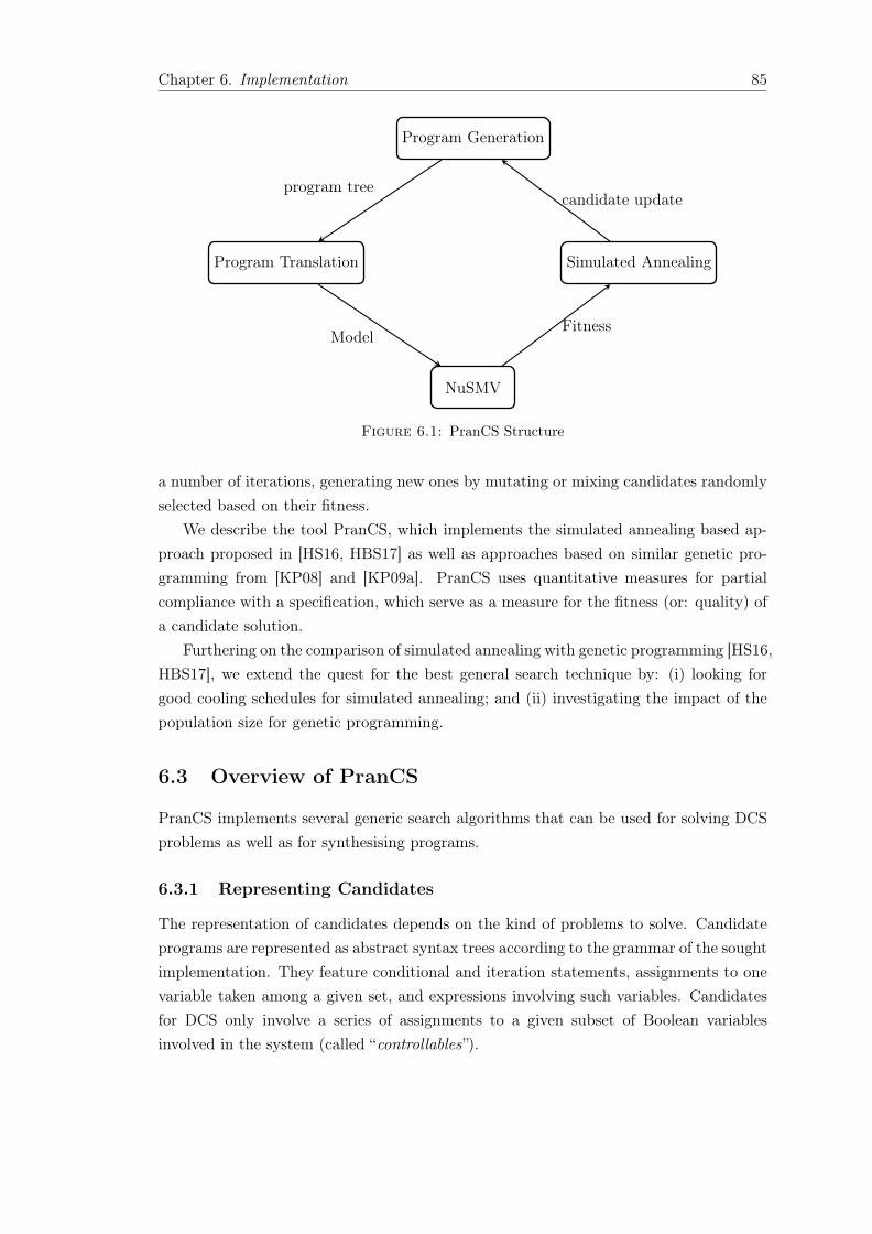
Chapter 6. Implementation 85
Program Generation
Program Translation
NuSMV
Simulated Annealing
program tree
ModelFitness
candidate update
Figure 6.1: PranCS Structure
a number of iterations, generating new ones by mutating or mixing candidates randomlyselected based on their fitness.
We describe the tool PranCS, which implements the simulated annealing based ap-proach proposed in [HS16, HBS17] as well as approaches based on similar genetic pro-gramming from [KP08] and [KP09a]. PranCS uses quantitative measures for partialcompliance with a specification, which serve as a measure for the fitness (or: quality) ofa candidate solution.
Furthering on the comparison of simulated annealing with genetic programming [HS16,HBS17], we extend the quest for the best general search technique by: (i) looking forgood cooling schedules for simulated annealing; and (ii) investigating the impact of thepopulation size for genetic programming.
6.3 Overview of PranCS
PranCS implements several generic search algorithms that can be used for solving DCSproblems as well as for synthesising programs.
6.3.1 Representing Candidates
The representation of candidates depends on the kind of problems to solve. Candidateprograms are represented as abstract syntax trees according to the grammar of the soughtimplementation. They feature conditional and iteration statements, assignments to onevariable taken among a given set, and expressions involving such variables. Candidatesfor DCS only involve a series of assignments to a given subset of Boolean variablesinvolved in the system (called “controllables”).
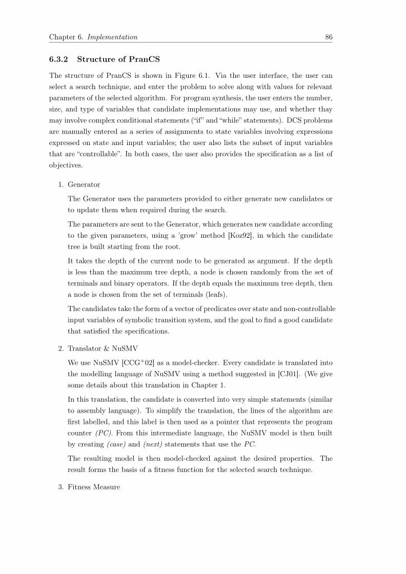
Chapter 6. Implementation 86
6.3.2 Structure of PranCS
The structure of PranCS is shown in Figure 6.1. Via the user interface, the user canselect a search technique, and enter the problem to solve along with values for relevantparameters of the selected algorithm. For program synthesis, the user enters the number,size, and type of variables that candidate implementations may use, and whether thaymay involve complex conditional statements (“if” and “while” statements). DCS problemsare manually entered as a series of assignments to state variables involving expressionsexpressed on state and input variables; the user also lists the subset of input variablesthat are “controllable”. In both cases, the user also provides the specification as a list ofobjectives.
1. Generator
The Generator uses the parameters provided to either generate new candidates orto update them when required during the search.
The parameters are sent to the Generator, which generates new candidate accordingto the given parameters, using a ’grow’ method [Koz92], in which the candidatetree is built starting from the root.
It takes the depth of the current node to be generated as argument. If the depthis less than the maximum tree depth, a node is chosen randomly from the set ofterminals and binary operators. If the depth equals the maximum tree depth, thena node is chosen from the set of terminals (leafs).
The candidates take the form of a vector of predicates over state and non-controllableinput variables of symbolic transition system, and the goal to find a good candidatethat satisfied the specifications.
2. Translator & NuSMV
We use NuSMV [CCG+02] as a model-checker. Every candidate is translated intothe modelling language of NuSMV using a method suggested in [CJ01]. (We givesome details about this translation in Chapter 1.
In this translation, the candidate is converted into very simple statements (similarto assembly language). To simplify the translation, the lines of the algorithm arefirst labelled, and this label is then used as a pointer that represents the programcounter (PC). From this intermediate language, the NuSMV model is then builtby creating (case) and (next) statements that use the PC.
The resulting model is then model-checked against the desired properties. Theresult forms the basis of a fitness function for the selected search technique.
3. Fitness Measure

Chapter 6. Implementation 87
The model checking results form the basis of a fitness function for the selectedsearch technique. To design a fitness measure for candidates, we make the hypoth-esis that the share of objectives that are satisfied so far by a candidate is a goodindication of its suitability w.r.t. the desired specification.
We additionally observe that weaker properties that can be mechanically derivedare useful to identify good candidates worth selecting for the generation of furtherpotential solutions. For example, if a property shall hold on all paths, it is betterif it holds on some path, and even better if it holds almost surely.
4. Search Technique
Based on the model checking results, we derive a quantitative measure for the fitness(as a level of partial correctness) of a candidate. The fitness measure obtained fora candidate is used as a fitness function for the selected search technique. If acandidate is evaluated as correct, we return (and display) it to the user.
Otherwise, depending on the search technique selected and the old and new fitnessmeasure/s, the current candidate or population is updated, and one or more candi-dates are sent for change to the Generator. The process is re-started if no solutionhas been found in a predefined number of steps (genetic programming) or whenthe cooling schedule expires (simulated annealing).
6.3.3 Selecting and Tuning Search Techniques
In terms of search techniques, PranCS implements the following methods: genetic pro-gramming, and simulated annealing. [KP09a] extends genetic programming by consider-ing the fitness as a pair of ‘safety-fitness’ and ‘liveness-fitness’, where the latter is onlyused for equal values of ‘safety-fitness’. Building upon this idea, we define two flavoursfor both simulated annealing and genetic programming: rigid (where the classic fitnessfunction is used) and safety-first, which uses the two-step fitness approach as above.
Further, genetic programming can be used with or without crossovers between can-didates [HS16, HBS17].
Depending on the selected search technique, the tool allows the user to input param-eters that control the dynamics of the synthesis process.
These parameters determine the likelihood of finding a correct program in each iter-ation and the expected running time for each iteration, and thus heavily influence theoverall search speed. For the genetic programming approach, the parameters include thepopulation size, the number of selected candidates, the number of iterations, and thecrossover ratio. For simulated annealing, the user chooses the initial temperature andthe cooling schedule.
Figure 6.2 shows the graphical user interface of PranCS.The input specification should be a list of NuSMV specifications. The tool will
produce weaker specifications for the purpose of producing a fitness measure.
Chapter 6. Implementation 88
Figure 6.2: Graphical User Interface. PranCS allows the user to fine-tune each searchtechnique by means of dedicated parameters.
Finally, the user defines the signature of the candidate by selecting input variablesthat are used to build the candidate that the user want to synthesise.
The model checker NuSMV is used for the individual model checking tasks. If thecandidate satisfied all required properties, then the synthesiser returns it as a correctcandidate. Otherwise, it will compare the fitness of the current candidate/s with the(stored) fitness value of the candidate/s it is derived from by mutation.
(This is the currently stored candidate or population.) The selection of the candidate/ population to be kept is determined by the selected generic search technique. Forsimulated annealing, if the fitness is lower, then the tool will update the stored candidatewith the probability defined by the loss in fitness and the current temperature taken fromthe cooling schedule.
If the fitness is not lower, the tool will always replaces the stored candidate by themutated one. When the end of the cooling schedule is reached, the tool aborts.
6.3.4 Parameters for Simulated Annealing
In simulated annealing (SA), the intuition is that, at the beginning of the search phase,the temperature is high, and it cools down as time goes by. The higher the temperature,the higher is the likelihood that a new candidate solution with inferior fitness replacesthe previous solution.
While this allows for escaping local minima, it can also happen that the candidatesdevelop into an undesirable direction. For this reason, simulated annealing does notcontinue for ever, but is re-started at the end of the cooling schedule.
Chapter 6. Implementation 89
Consequently, there is a sweet-spot in just how long a cooling schedule should be andwhen it becomes preferable to re-start, but this sweet-spot is difficult to find. We reportour experiments with PranCS for tuning the cooling schedule in Section 6.4.
6.3.5 Parameters for Genetic Programming
For genetic programming (GP), the parameters are the initial population size, the crossovervs mutation ratio, and the fitness measure used to select the individuals. The populationsize affects the algorithm in two ways: larger populations could provide better diversity.However, it also increases the number of iterations required to find a good solution. Weinvestigate how the population size and crossover ratio affect the performance of thesealgorithms.
6.4 Exploration of the Parameter Space
In [HS16], we have used our techniques to generate correct solutions for mutual exclu-sion and leader election problems; we have then exercised the same techniques to solvescalable DCS problems [HBS17]. In both cases, and with parameter values borrowedfrom [KP09a, KP08], we could already accelerate synthesis significantly using simulatedannealing compared to genetic programming (by 1.5 to 2 orders of magnitude).
In this work, our aim is to further explore the performance impact of the parametersfor each search technique. We thus reuse the same scalable benchmarks as in [HS16,HBS17]1: program synthesis problems consist of mutual exclusion (“2/3 shared bits”)and leader election (“3/4 nodes”); DCS problems compute controllers enforcing mutualexclusions and progress between 1 to 6 tasks modelled as automata (“1/6-Tasks”).
6.4.1 Exploring Population Size & Crossover Ratio
We have carried out several experiments in order to investigate how the population sizeand crossover ratio effect our synthesis approach when using genetic programming, withvarying population sizes; details of our results are presented in Chapter 3 and Chapter 4.Although results indicate that some crossover ratio that is good in general may exist, thenegative impact of small population sizes on success rates can in practice be mitigatedby the faster execution times.
We found that the initial population size dramatically increases the overall expectedtime for finding a good solution.
Continuing on our investigations of the parameters, the "best" initial population sizeand crossover ratio are fixed and a new measure for the fitness applied.
1In all tables, execution times are in seconds; t is the mean execution time of single executions(succeeding or failing), and columns “expec. time” extrapolate t based on the success rate obtained in100 single executions (“suc. %”).

Chapter 6. Implementation 90
Search Tech. t suc. % expec. time1-Task Rigid SA 20 13 153
Safety-first SA 19 16 118
2-Tasks Rigid SA 25 10 250Safety-first SA 24 13 184
3-Tasks Rigid SA 33 9 366Safety-first SA 29 10 290
4-Tasks Rigid SA 47 9 522Safety-first SA 43 9 477
5-Tasks Rigid SA 76 8 950Safety-first SA 70 9 777
6-Tasks Rigid SA 119 7 1,700Safety-first SA 106 7 1,514
Table 6.1: Synthesis times with the best parameters observed for Simulated Annealingapplied to our DCS benchmarks
|P | slctd cand. t suc. % expec. time
1505 138 15 9207 139 15 9269 139 14 992
2505 218 19 11477 218 19 11479 218 19 1147
3505 340 24 14167 340 24 14169 340 24 1416
Table 6.2: On the left: Safety-first GP with crossover for DCS (2-Tasks only), withVarious Population Sizes (|P |).
6.4.2 Exploring Cooling Schedules
We have studied good temperature ranges by keeping the temperature constant duringa “cooling” schedule with 25,000 steps. We give the results of these experiments inChapter 3 and Chapter 4. A robust temperature sweet-spot clearly exists for our scalablebenchmarks, suggesting that the quest for robust and generic good cooling schedules isworth pursuing.
Adaptive cooling schedule enables the decrease of the temperature to be low whenreach a good temperature otherwise it decremented normally. We have set the initialtemperature to 20, 000. The cooling schedule decreases the temperature by 0.8 in eachiteration in the normal movement and decrease it by 0.2 in the good temperature,
6.5 Conclusion
The results from [HS16, HBS17] already turn in favour of simulated annealing over theother general search technique we have studied.
These results shown on Table 6.2 (given in % and seconds, respectively, with thebest values in bold) indicate that using simulated annealing with an adaptive coolingschedule slightly increase the single execution time and also overall time. We use ascalable example of DCS problem from [HBS17] each problem N-Tasks was built usingN instances.

Chapter 6. Implementation 91
Together with our extensive exploration of the parameter space, the evaluation ofPranCS indicates that simulated annealing is faster that genetic programming (we re-port some synthesis times with the best parameters observed for simulated annealing inTable 6.2), and that some temperature ranges are more useful than others.
In order to integrate this result into the cooling schedule we plan to use an adaptivecooling schedule, in which the decrements of the temperature depends on the improve-ment of the fitness.

Chapter 7
Conclusion
This chapter provides a summary of the research work described in this thesis, the mainfindings together with the contributions. The rest of this section is organised as follows:Section 7.1 provides a summary of the work presented while Section 7.2 presents themain findings in the context of the research question and research motivations identifiedin Chapter 1.
7.1 Summery
We have implemented an automated programming technique based on simulated an-nealing and genetic programming, both in the pure form of and the arguably hybridform.
The results are very clear and in line with the expectation we had drawn from theliterature [Dav87, LMST96, MS96]. When crossovers are not used, the main differencebetween the established genetic programming techniques and simulated annealing is thesearch strategy of using many and using a single instance, respectively. The data gatheredconfirms that an increase of the number of iterations can easily overcompensate thebroader group of candidates kept in genetic programming. In our experiments, we haveused an increase that fell short of creating the same expected running time for a singlefull execution (with or without success), and yet outperformed even the hybrid approachw.r.t. the success rate on three of our four benchmarks. We have also added variations ofgenetic programming that include crossover to validate the assumption that crossovers donot lead to an annihilation of the advantage, but it proved that the hybrid approach, andthus the stronger competitor, does not benefit much from using crossover. The doubleadvantage of shorter running time and higher success rate led to an improvement of1.5 to 2 orders of magnitude compared to pure genetic programming (with and withoutcrossover), and between half an order and one order of magnitude when compared to thehybrid approach (with or without crossover).
The results from [HS16] indicate that simulated annealing is the better general searchtechnique to use. It will be interesting to see if these factors are essentially constant, orif they depend heavily on the circumstances. Together with the later extensions, the tool
93
Chapter 7. Conclusion 94
evaluation indicates that there are good temperature ranges. Inspired by our previousinvestigations for program synthesis using general search techniques [HS16], and in aneffort to inquire further applications of such techniques, we have defined a class of DCSproblems where deterministic strategies are sought. We adapted our algorithms to seeksolutions for these problems, and conducted an experimental evaluation using a scalableinstance of a DCS problem. Results proved to be consistent with our assumption thatthe relative performance of the algorithms would match our previous results for programsynthesis.
7.2 Main Findings and Contributions
This section presents the main findings from the research work presented in this thesis.In order to answer the research question from Section 1.3, the resolution of a number ofsubsidiary research questions was required. The work described in the thesis addresseseach of these research questions as follows:
• General Search Technique: What is the best search technique that can be usedfor program synthesis? Is genetic programming, simulated annealing, or a hybridof them better? can we implement them in another way as hybrid methods?
We use a formal verification technique, model checking, as a way of assessing itsfitness in an inductive automatic programming system. We have implemented asynthesis tool, which uses multiple calls to the model checker NuSMV to determinethe fitness for a candidate program. The candidate programs exist in two forms.The main form is a simple imperative language. This form is subject to mutation,but it is translated to a secondary form, the modeling language of NuSMV, forevaluating its fitness. All choices of how exactly a program is represented andhow exactly the fitness is evaluated are disputable. Generic search techniques are,however, usually rather robust against changes in such details. While there hasbeen further research on how to measure partial satisfaction, we believe that thebest choice for us is to keep to the choices made for promoting genetic program-ming, as this is the only choice that is completely free of suspicion of being selectedfor being more suitable for simulated annealing than for genetic programming. Asecond motivation for this selection is that it results in very simple specificationsand, therefore, in a fast evaluation of the fitness. Noting that synthesis entails onaverage hundreds of thousands to millions of calls to a model checker, only simpleevaluations can be considered. We have implemented six different combinations ofselection and update mechanism to test our hypothesis: besides simulated anneal-ing, we have used genetic programming both without crossover and with crossover.The tests we have run confirmed that simulated annealing performs significantlybetter than genetic programming. As a side result, we found that the assumptionof the authors of [KP08, KP09a, KP09b] that crossover does not accelerate genetic

Chapter 7. Conclusion 95
programming did not prove to be entirely correct, but the advantages we observedwere minor.
• Search Techniques Parameters: What are the efficient parameters that canbe used for genetic programming and simulated annealing? Is the application ofcrossover effective? How does initial population size affect the cost beside thesuccess rate? How does the initial temperature and cooling schedule affect theresults of simulated annealing? Are there ’best’ parameters for our techniques?
Besides serving as a synthesis tool, the main intention of PranCS is to allow fora comparison of different generic search techniques. In [HS16], we have used ourtechnique to generate correct solutions for mutual exclusion and leader electionand found that simulated annealing is much (1.5 to 2 orders of magnitude) fasterthan genetic programming.
• Controller Synthesis: Can we use the same techniques in controller synthesis?Are the results similar to those of program synthesis? What about the parametersdo they have the same effect?
We have defined a class of DCS problems where deterministic strategies are sought.We adapted our algorithms to seek solutions for these problems, and conductedan experimental evaluation using a scalable instance of a DCS problem. Resultsproved to be consistent with our assumption that the relative performance of thealgorithms would match our previous results for program synthesis. Yet, our imple-mentations are proofs of concept, and one can think of numerous practical improve-ments that constitute inescapable ways to pursue investigating efficient symbolicDCS algorithms using simulated annealingFor instance, canonically representingsymbolic candidate strategies using BDDs instead of syntactic trees would allowfor building a cache of fitness results, and thereby avoid re-evaluating the fitnessof equivalent candidate strategies.
Similarly, implementing the algorithms in a symbolic model-checker could permit toavoid the very costly—and often performance bottleneck in case of model-checkersusing BDDs—reconstruction of symbolic representations at every iteration of thealgorithms. Finally, note that our search based algorithms do not require thecomputation of the unsafe region to produce deterministic strategies. Hence, con-sidering the current advances in model-checking technologies, our algorithms mightconstitute ways to solve DCS problems on some classes of infinite-state systems forwhich the unsafe region cannot be computed.
• Synthesis Tool: What is the scope of a synthesis tool based on generic searchtechnique?
We have developed PranCS, which is a tool for protocol and controller synthesis.It exploits general search techniques such as simulated annealing and genetic pro-gramming for homing in on an implementation, and use model checking for the

Chapter 7. Conclusion 96
fitness function. We use NuSMV as a back-end for the individual model check-ing tasks and a simple candidate mutator to drive the search. Our Proctocol andController Synthesis (PranCS) tool is designed to explore the parameter spaceof different synthesis techniques. Besides using it to synthesise a discrete controlstrategy for reactive systems (controller synthesis) and for protocol adapters for thecoordination of different threads (protocol synthesis), we can also use it to studythe influence of turning various screws in the synthesis process. For simulated an-nealing, PranCS allows the user to define the behaviour of the cooling schedule.For genetic programming, the user can select the population size. Additionally,PranCS offers different automated techniques to quantify partial compliance witha specification and to infer the fitness of a candidate implementation based on thispartial compliance. PranCS also allows for choosing small random seeds as well asuser defined seeds to allow the user to define a starting point for the search, e.g.for candidate repair.
The main contributions of the research presented in this thesis were presented inChapter 1. These are restated here, for completeness, as follows:
7.2.1 Program synthesis
In this part of our work we suggest to:
1. Use simulated annealing for program synthesis and compare it to similar approachesbased on genetic programming.
2. Use a formal verification technique, model checking, as a way of assessing its fitnessin an inductive automatic programming system.
3. We have implemented a synthesis tool, which uses multiple calls to the modelchecker NuSMV [CCG+02] to determine the fitness of a candidate program.
4. We have implemented six different combinations of selection and update mecha-nism to test our hypothesis: besides simulated annealing, we have used geneticprogramming both without crossover (as discussed in [KP08, KP09a, KP09b]) andwith crossover and Hybrid genetic programming both without crossover (as dis-cussed in [KP08, KP09a, KP09b]) and with crossover.
The tests we have run confirmed that simulated annealing performs significantly bet-ter than genetic programming. As a side result, we found that the assumption of theauthors of [KP08, KP09a, KP09b] that crossover does not accelerate genetic program-ming did not prove to be entirely correct, but the advantages we observed were minor.
7.2.2 Controller synthesis
1. We first define a symbolic model and an associated class of DCS problems, forwhich deterministic strategies are sought.

Chapter 7. Conclusion 97
2. Next, we adapt the aforementioned search techniques to obtain algorithmic solu-tions that avoid computing the unsafe portion of the state-space.
3. Then, we confirm the hypotheses that: (i) general search techniques are as appli-cable to solve our DCS problem as they are for synthesising programs; and (ii) oneobtains similar relative performance results for our DCS problem. experimental re-sults [HS16] for program synthesis , essentially that simulated annealing performsbetter than genetic programming.
4. To assess these hypotheses, we adapt the six different combinations of candidateselection and update mechanisms of our previous work [HS16], and execute themon a scalable example DCS problem.
5. perform an experimental feasibility assessment.
From the performance results we obtain, we draw the conclusion that , even thoughfor technical reasons our current experimental results do not compare favourably withexisting symbolic DCS tools, simulated annealing, when combined with efficient model-checking techniques, is worth further investigating to solve symbolic DCS problems.
As noted in Section 4.7, our experimental results do not compare favourably withexisting symbolic DCS tools.


Bibliography
[ACMR03] Karine Altisen, Aurélie Clodic, Florence Maraninchi, and Eric Rutten. Us-ing controller-synthesis techniques to build property-enforcing layers. InProgramming Languages and Systems: 12th European Symposium on Pro-gramming, ESOP 2003 Held as Part of the Joint European Conferences onTheory and Practice of Software, ETAPS 2003 Warsaw, Poland, April 7–11,2003 Proceedings, pages 174–188, Berlin, Heidelberg, 2003. Springer BerlinHeidelberg.
[AHM+98] Rajeev Alur, Thomas A. Henzinger, Freddy Y. C. Mang, Shaz Qadeer, Sri-ram K. Rajamani, and Serdar Tasiran. Mocha: Modularity in model check-ing. In Proceedings of the 10th International Conference on Computer AidedVerification, CAV ’98, pages 521–525, London, UK, UK, 1998. Springer-Verlag.
[AMP95] Eugene Asarin, Oded Maler, and Amir Pnueli. Symbolic controller synthesisfor discrete and timed systems. In Hybrid Systems II, pages 1–20, Berlin,Heidelberg, 1995. Springer Berlin Heidelberg.
[BCM+90] Jerry R. Burch, Edmund M. Clarke, Kenneth L. McMillan, David L. Dill,and L. J. Hwang. Symbolic model checking: 10ˆ20 states and beyond. pages428–439, 1990.
[BM14] Nicolas Berthier and Hervé Marchand. Discrete Controller Synthesis forInfinite State Systems with ReaX. In 12th Int. Workshop on Discrete EventSystems, WODES ’14, pages 46–53. IFAC, May 2014.
[BMM13] Nicolas Berthier, Florence Maraninchi, and Laurent Mounier. SynchronousProgramming of Device Drivers for Global Resource Control in EmbeddedOperating Systems. ACM Trans. Embed. Comput. Syst., 12(1s):39:1–39:26,March 2013.
[Bry86] Randal E. Bryant. Graph-based algorithms for boolean function manipula-tion. IEEE Trans. Comput., 35(8):677–691, August 1986.
[CCG+02] Alessandro Cimatti, Edmund M. Clarke, Enrico Giunchiglia, FaustoGiunchiglia, Marco Pistore, Marco Roveri, Roberto Sebastiani, and Armando
99

Bibliography 100
Tacchella. NuSMV 2: An opensource tool for symbolic model checking. InIn CAV, LNCS 2404, pages 359–364. Springer, 2002.
[CE82] Edmund M. Clarke and E. Allen Emerson. Design and synthesis of synchro-nization skeletons using branching time temporal logic. In IBM Workshopon Logics of Programs, volume 131 of LNCS, pages 52–71. Springer, 1982.
[CGP99] Edmund M. Clarke, Jr., Orna Grumberg, and Doron A. Peled. Model Check-ing. MIT Press, Cambridge, MA, USA, 1999.
[CJ01] John A. Clark and Jeremy L. Jacob. Protocols are programs too: the meta-heuristic search for security protocols. Information and Software Technology,43:891–904, 2001.
[CKN98] José ER Cury, Bruce H Krogh, and Toshihiko Niinomi. Synthesis of supervi-sory controllers for hybrid systems based on approximating automata. IEEETransactions on Automatic Control, 43(4):564–568, 1998.
[Con90] D.T. Connolly. An improved annealing scheme for the qap. In European J.of Operational Research, volume 46, pages 93 –100, 1990.
[Dav87] Lawrence Davis. Genetic Algorithms and Simulated Annealing. Morgan Kauf-mann Publishers Inc., 1987.
[Dij65] E. W. Dijkstra. Solution of a problem in concurrent programming control.Commun. ACM, page 569, 1965.
[DKL15] Cristina David, Daniel Kroening, and Matt Lewis. Using program synthe-sis for program analysis. In LPAR, volume 9450 of LNCS, pages 483–498.Springer, 2015.
[Ehl11] Rüdiger Ehlers. Unbeast: Symbolic bounded synthesis. In Tools and Al-gorithms for the Construction and Analysis of Systems: 17th InternationalConference, TACAS 2011, Held as Part of the Joint European Conferenceson Theory and Practice of Software, ETAPS 2011, Saarbrücken, Germany,March 26–April 3, 2011. Proceedings, pages 272–275, Berlin, Heidelberg,2011. Springer Berlin Heidelberg.
[Eme90] E. Allen Emerson. Temporal and modal logic. In Jan van Leeuwen, editor,Handbook of Theoretical Computer Science (Vol. B), pages 995–1072. MITPress, Cambridge, MA, USA, 1990.
[FJR09] Emmanuel Filiot, Naiyong Jin, and Jean-François Raskin. An antichain algo-rithm for ltl realizability. In Computer Aided Verification: 21st InternationalConference, CAV 2009, Grenoble, France, June 26 - July 2, 2009. Proceed-ings, pages 263–277, Berlin, Heidelberg, 2009. Springer Berlin Heidelberg.

Bibliography 101
[FPS15] John Fearnley, Doron Peled, and Sven Schewe. Synthesis of succinct systems.Journal of Computer and System Sciences, 81(7):1171–1193, 2015.
[FS05] Bernd Finkbeiner and Sven Schewe. Uniform distributed synthesis. In LICS,pages 321–330. IEEE Computer Society Press, 2005.
[FS13] Bernd Finkbeiner and Sven Schewe. Bounded synthesis. International Jour-nal on Software Tools for Technology Transfer, 15(5-6):519–539, 2013.
[GR09] Alain Girault and Éric Rutten. Automating the addition of fault toler-ance with discrete controller synthesis. Formal Methods in System Design,35(2):190, 2009.
[HBS17] Idress Husien, Nicolas Berthier, and Sven Schewe. A hot method for synthe-sising cool controllers. In Proceedings of the 24th ACM SIGSOFT Interna-tional SPIN Symposium on Model Checking of Software, SPIN 2017, pages122–131, New York, NY, USA, 2017. ACM.
[HJJ03] Darrall Henderson, Sheldon H Jacobson, and Alan W Johnson. The theoryand practice of simulated annealing. In Handbook of metaheuristics, pages287–319. Springer, 2003.
[HO13] Thomas A. Henzinger and Jan Otop. From model checking to model mea-suring. In CONCUR, volume 8052 of LNCS, pages 273–287. Springer, 2013.
[HRL08] Yann Hietter, Jean-Marc Roussel, and Jean-Jacques Lesage. Algebraic Syn-thesis of Transition Conditions of a State Model. In 9th International Work-shop on Discrete Event Systems, WODES ’08, pages 187–192. IEEE, May2008.
[HS16] Idress Husien and Sven Schewe. Program generation using simulated anneal-ing and model checking. In SEFM, volume 9763 of LNCS, pages 155–171,2016.
[HSB17] Idress Husien, Sven Schewe, and Nicolas Berthier. Prancs: A protocol anddiscrete controller synthesis tool. In Dependable Software Engineering. Theo-ries, Tools, and Applications - Third International Symposium, SETTA 2017,Changsha, China, October 23-25, 2017, Proceedings, pages 337–349, 2017.
[JGB05] Barbara Jobstmann, Andreas Griesmayer, and Roderick Bloem. Programrepair as a game. In CAV, volume 3576 of LNCS, pages 226–238. Springer,2005.
[Joh07] Colin G. Johnson. Genetic programming with fitness based on model check-ing. In EuroGP, volume 4445 of LNCS, pages 114–124. Springer, 2007.
[KH91] Bruce H Krogh and Lawrence E Holloway. Synthesis of feedback control logicfor discrete manufacturing systems. Automatica, 27(4):641–651, 1991.

Bibliography 102
[Koz92] John R. Koza. Genetic Programming: On the Programming of Computers byMeans of Natural Selection. MIT Press, Cambridge, MA, USA, 1992.
[KP08] Gal Katz and Doron Peled. Model checking-based genetic programming withan application to mutual exclusion. In TACAS, volume 4963 of LNCS, pages141–156. Springer, 2008.
[KP09a] Gal Katz and Doron Peled. Model checking driven heuristic search for correctprograms. InMoChArt, volume 5348 of LNCS, pages 122–131. Springer, 2009.
[KP09b] Gal Katz and Doron Peled. Synthesizing solutions to the leader electionproblem using model checking and genetic programming. In HVC, volume6405 of LNCS, pages 117–132. Springer, 2009.
[KV99] Orna Kupferman and Moshe Y. Vardi. Church’s problem revisited. TheBulletin of Symbolic Logic, 5(2):245–263, June 1999.
[KV01] Orna Kupferman and Moshe Y. Vardi. Synthesizing distributed systems. InLICS, pages 389–398. IEEE Computer Society Press, 2001.
[LMST96] Jussi Lahtinen, Petri Myllymäki, Tomi Silander, and Henry Tirri. Empiricalcomparison of stochastic algorithms. In 2NWGA, pages 45–60, 1996.
[LP85] Orna Lichtenstein and Amir Pnueli. Checking that finite state concurrentprograms satisfy their linear specification. In POPL, pages 97–107. ACM,1985.
[MBLL00] Hervé Marchand, Patricia Bournai, Michel Le Borgne, and Paul Le Guer-nic. Synthesis of discrete-event controllers based on the signal environment.Discrete Event Dynamic System: Theory and Applications, 10(4):325–346,October 2000.
[MS96] J.W. Mann and G.D. Smith. A comparison of heuristics for telecommuni-cations traffic routing. In Modern Heuristic Search Methods, pages 235–254,1996.
[MS00] Hervé Marchand and Mazen Samaan. Incremental Design of a Power Trans-former Station Controller Using a Controller Synthesis Methodology. IEEETrans. Softw. Eng., 26:729–741, August 2000.
[MT01] P. Madhusudan and P. S. Thiagarajan. Distributed controller synthesis for lo-cal specifications. In ICALP, volume 2076 of LNCS, pages 396–407. Springer,2001.
[Pnu77] Amir Pnueli. The temporal logic of programs. In FOCS, pages 46–57. IEEEComputer Society Press, 1977.

Bibliography 103
[PR90] Amir Pnueli and Roni Rosner. Distributed reactive systems are hard tosynthesize. In FOCS, pages 746–757. IEEE Computer Society Press, 1990.
[RCK+09] Leonid Ryzhyk, Peter Chubb, Ihor Kuz, Etienne Le Sueur, and GernotHeiser. Automatic device driver synthesis with termite. In Proceedings of theACM SIGOPS 22nd Symposium on Operating Systems Principles, SOSP ’09,pages 73–86, New York, NY, USA, 2009. ACM.
[RW89] Peter J. G. Ramadge and W. Murray Wonham. The control of discrete eventsystems. Proceedings of the IEEE; Special issue on Dynamics of DiscreteEvent Systems, 77(1):81–98, 1989.
[SF06] Sven Schewe and Bernd Finkbeiner. Synthesis of asynchronous systems. InLOPSTR 2006, volume 4407 of LNCS, pages 127–142. Springer, 2006.
[Sol13] Armando Solar-Lezama. Program sketching. International Journal on Soft-ware Tools for Technology Transfer, 15(5-6):475–495, 2013.
[vEJ13] Christian von Essen and Barbara Jobstmann. Program repair without regret.In CAV, volume 8044 of LNCS, pages 896–911. Springer, 2013.
[WLK+09] Yin Wang, Stéphane Lafortune, Terence Kelly, Manjunath Kudlur, and ScottMahlke. The theory of deadlock avoidance via discrete control. In Proceedingsof the 36th annual ACM SIGPLAN-SIGACT Symposium on Principles ofProgramming Languages, POPL ’09, pages 252–263, New York, NY, USA,2009. ACM.
[ZD12] MengChu Zhou and Frank DiCesare. Petri net synthesis for discrete eventcontrol of manufacturing systems, volume 204. Springer Science & BusinessMedia, 2012.