Reputation and monitoring ability in loan syndications *

Hua Jessie Zhang**

September 24th, 2003

* JEL classification: G21. Key words: Loan syndication, asymmetric information. The author would like to thank her supervisor, Professor Gordon S. Roberts, for his support and advice. The author also would like to thank Kin Chung Lo, Kamphol Panyagometh, Jonathan Yan, Matthew Bowler as well as Stephen Sapp for their helpful comments and suggestions. All errors are the responsibility of the author.

** Ph.D. Candidate, Schulich School of Business, Finance Area, York University, 4700 Keele Street, Toronto, Ontario, Canada, M3J 1P3. Phone: 416-736-2100 Ext: 20635. Email: hjzhang@ssb.yorku.ca.

Reputation and monitoring ability in loan syndications

Abstract

Syndicated loans are an increasingly important financial instrument, occupying

40% of the US corporate finance market today. Employing a combination of modeling

and empirical testing, we provide and confirm the mechanics of how information about

the true motive and monitoring ability of lead banks is updated from a market perspective

through a sequence of loan syndication decisions. A repeated Bayesian game model with

incomplete information for syndicate members is constructed followed by empirical tests

to support the model. Further, lead banks are divided into two groups: “active” and

“drop-out” groups. Advancing upon previous study, we propose that the actions of the

“active” group should be consistent with the reputation hypothesis, while those of the

“drop-out” group could be motivated by either the exploitation effect or the

overconfidence effect. Two testable hypotheses to discriminate between the two effects

are proposed. The empirical results of this study confirm that the actions of the “active”

group are consistent with the reputation hypothesis and those of the “drop-out” group are

consistent with the overconfidence hypothesis.

1

Reputation and monitoring ability in loan syndications

I. Introduction

A syndicated loan is one in which a syndicate of lenders consisting of two or

more banks contracts with a borrower to provide loans on common terms and conditions

governed by a set of common documents (Syndicated Lending (2000)). By the late

1990s syndicated loans had become a rapidly growing emerging market, and an

increasingly important financing tool.

Syndicated loans possess qualities of both public and private debt. Public debt

tends to be long-term, with relatively loose covenants, and in most cases cannot be

renegotiated. By contrast, bank loans tend to be shorter term, with extensive covenants,

and can be restructured. Berlin and Loeys (1988), Berlin et al. (1992), and Rajan et al.

(1995) examined and confirmed these contractual characteristics extensively. A

syndicated loan has characteristics of both public and private debt, as it is the sale of a

“bundle” of loans to a group of institutional participants. In contrast, a non-syndicated

bank loan sells a “whole” contract to a borrower.

The syndicate of participating lenders delegates some monitoring responsibility to

the lead bank(s) prior to finalization of the loan syndication. The loan agreement

specifies which decisions require the consent of certain proportions of the member banks.

A standard syndicated loan agreement usually requires unanimous agreement for any

reduction in fees, principal, interest, or for changes in the terms of credits. However,

2

there are provisions that allow the lead bank to declare a default event, typically after

consulting with the other syndicate members.

Loan syndication invites agency problems such as adverse selection and moral

hazard. As mentioned by Esty (2001), the banks invited to participate in the loan

syndication are usually not banks with a previous relationship with the borrower, but

rather banks with a prior syndication relationship with the lead bank. An example of

asymmetric information is also illustrated by Simon (1993): since the syndicate

participants rely mainly on the borrower credit information contained in documents

provided by the lead bank, the lead bank may have additional inside information about

the borrower unavailable to the syndicate members. For example, in cases where the

borrower has been a long-time customer of the lead bank, the lead bank might have some

information not reflected in the borrower’s public financial statements. Dennis and

Mullineaux (2000) give a few examples of such information, citing “judgments

concerning management expertise, the nature of customer-supplier relationships, or the

borrower’s capacity to adapt successfully to changing market conditions.” Because loan

syndication involves relationship banking and significant amounts of underwriting

revenue, the originating banks may have incentives to syndicate loans even when the

inside information is not favorable, thereby creating an adverse selection problem.

Loan syndication also involves moral hazard, as Gorton and Pennachi (1995) and

Dennis and Mullineaux (2000) have pointed out. Once it is sold to syndicate participants,

the participants’ portion of the loan is removed from the balance sheets of the lead banks

and appears on the syndication participants’ statements. As a result, the burden of the

incentive to monitor the loan is shifted from the lead bank to the syndication participants.

3

Dennis and Mullineaux (2000) were the first to study the factors affecting the

decision to syndicate a loan and, in cases of loan syndication, the percentage of the loan

syndicated to participating members. Using the DealScan database from the Loan Pricing

Corporation (LPC), they found that the decision to syndicate a loan, together with the

percentage syndicated out to participating members, is affected from the degree of

transparency of the borrower, the loan and lead bank characteristics and the reputation of

the lead banks as syndication originators. In particular, the more transparent the borrower

is, as evidenced by the existence of a credit rating or by being listed on a stock exchange,

the more likely the loan is to be syndicated and sold in greater proportions to syndication

participants.

In the same vein, Panyagometh and Roberts (2003) proposed two alternative

hypotheses to explain loan syndication behavior in general: a reputation hypothesis

versus an exploitation hypothesis. Under the reputation hypothesis, lead banks would try

to syndicate quality loans, signaling their position as “certifiers of quality loans” for

future loan syndication. They used new information measures to re-examine the factors

affecting decision-making for loan syndication and the percentage of loans syndicated out

to other syndication members. Their empirical findings are consistent with the reputation

hypothesis. They also found that the addition of a performance pricing feature linking a

loan’s prime or LIBOR spread to the subsequent financial performance of the borrower,

as measured by various financial ratios, helps to mitigate information asymmetries within

loan syndicates. As a result, the addition of such a performance pricing feature facilitates

the formation of loan syndicates.

4

In both Dennis and Mullineaux (2000) and Panyagometh and Roberts (2003), the

findings confirm the belief that “scale and scope of information asymmetries are relevant

to the ‘salability’ of a debt contract” (Dennis and Mullineaux (2000)). These prior studies

also consistently found that a reputation effect is relevant to both decisions. In other

words, more reputable lead banks are more likely to syndicate, and when they do,

syndicate greater proportions of higher quality loans.

However, neither study investigates precisely how reputation functions at the

theoretical level or what kind of information can be deemed to be associated with a

negative/positive reputation. The information measures in Dennis and Mullineaux (2000)

and Panyagometh and Roberts (2003) did not discriminate between positive and negative

reputation effects, nor did these studies investigate the mechanics of how the other

syndicate members learn about the lead bank from previous syndications, or how a

syndicate member’s information about the lead bank(s) is updated before decision-

making. The theoretical model in our paper addresses the questions, connecting and

explaining past empirical work on a theoretical level. The empirical part of our paper,

together with the previous empirical work of Dennis and Mullineaux (2000) and

Panyagometh and Roberts (2003) can be considered as confirmations of the model.

In addition, furthering the reputation versus exploitation hypothesis developed by

Panyagometh and Roberts (2003) for the syndication market as a whole, we view lead

banks as falling into two groups. The “active” group is defined as lead banks that were

still initiating syndicated loans in 1998 or after, or whose parent firms were still doing so.

The “drop-out” group is defined as lead banks that had previously been in the origination

market for loan syndication but ceased acting as a lead bank in 1998 and after. We

5

propose that the “active” group should be consistent with reputation hypothesis, while the

“drop-out” group could be subject to either the exploitation hypothesis or the

overconfidence hypothesis.

Good monitoring ability is usually implicitly assumed in previous work studying

asymmetric information between lead banks and participating members. Hubbard et al.

(2002), among others, pointed out that banks have a cost advantage over non-bank

financial institutions and, therefore, better ability to monitor the financial health of these

relational clients. The reputation hypothesis and the exploitation hypothesis from

Panyagometh and Roberts (2003) implicitly assume that lead banks have sufficient

monitoring ability either to establish their reputation as a certifier of quality loans or to

exploit their inside information about the borrower. However, in reality this might not be

the case. In this paper we also extend previous work by incorporating an overconfidence

hypothesis, which has until now been ignored. Under the overconfidence hypothesis, the

reason lead banks drop out and abdicate their leading roles could be that they over-

estimate their ability to monitor the borrowers. As a result of this overconfidence, more

loans turn out to be “bad” than expected. Consequently, both lead banks and participating

members suffer from more loan defaults than expected. We also conduct tests for both

the exploitation and the overconfidence hypotheses for the “drop-out” group.

In this paper, a repeated Bayesian game with incomplete information for

syndicate participants is constructed for the syndicated loan decision-making process. In

each period, from a syndicate member’s perspective, only one of two possible situations

(states) can occur. In the first situation, the lead bank does not exploit inside information

about the borrower, which is usually a relational client of the lead bank, and the lead bank

6

also has adequate ability to monitor the borrower. In the second situation (state) the lead

bank either exploits its inside information about the borrower or is overconfident about

its monitoring ability. The potential syndicate participant does not know which is the

true state, but assigns a probability to each state. In each period, the syndicate

participants learn about the quality of loans in all previous periods, and update their

beliefs about the motives and the monitoring ability of the lead bank by updating the

probability of these two states. By comparing the two payoffs using the updated

probabilities, syndicate members then decide whether to become involved in syndication.

We also introduce two new variables associated with lead bank reputation and

changes in borrower financial status. The first new variable, TOTAL, serves as an

improved measure of the lead bank’s reputation as a loan syndication originator. Dennis

and Mullineaux (2000) used several proxies for the reputation effect: the number of

syndication originations conducted in the pre-sample period by the lead bank syndicating

the loan (REPEAT), and a dummy variable indicating whether the managing agent is a

bank (BANK). REPEAT is calculated based on the number of loan syndications

originated by the lead bank before January 1st, 1987, the pre-sample period before the

regression sample. REPEAT might not be a strong indicator of reputation within the

regression sample, although it does reflect some information from the pre-sample period.

Also it does not discriminate between “good” syndications and “bad” syndications. The

dummy variable BANK can only distinguish between bank and non-bank originators, not

between different bank originators. Panyagometh and Roberts (2003) used AVGVOL as

the measure of lead bank reputation. AVGVOL is the yearly average dollar amount of

syndicated loans previously originated by the lead bank. It still suffered from the same

7

problem of not being able to discriminate between “good” and “bad” loan syndications in

the past.

The new variable used in this paper, ZCHAG, serves as an improved measure of

financial health changes experienced by the borrower. Panyagometh and Roberts (2003)

used ZSCORECHG in their robustness test. ZSCORECHG is a dummy variable that

equals 1 if the change in Z score is positive and –1 if the change is negative. As a

dummy variable, ZSCORECHG can exaggerate minor random noise caused by factors

irrelevant to the financial status of the borrower. For example, it is an overstatement to

assume a -0.05% Z score change would have the same effect on syndication decision-

making as a –200% Z score change. Instead, we define our new continuous variable

ZCHAG as the change in a borrower’s Altman’s Z score one year after the loan is closed,

which solves the problem of non-proportionality in the variable.

An improved Z score change will have implications for the possibility of loan

default that are the opposite of those of a deteriorated Z score change ZCHAG can,

therefore, also be considered as a proxy for changes in loan quality. Next, we define

“good” loans as loans whose borrowers end up with unchanged1 or improved Z scores

one year after the loans were initiated, and “bad” loans as loans whose borrowers end up

with deteriorated Z scores one year after loans are initiated.

In this paper, a new and more accurate measurement of the reputation effect of the

lead banks, TOTAL, is used. TOTAL is the number of prior syndications conducted by

the lead bank that turned out to be “good” loans, minus the number that turned out to be

“bad” loans. Compared to reputation proxies used in prior studies, TOTAL is a more

advanced, dynamic measure of syndication reputation as it accumulates over time, which 1 Unchanged Z score is defined here as Z score with change greater than -15%.

8

is able to discriminate and, further, reward past “good” loan syndication and penalize past

“bad” loan syndication by the lead bank. As a result, it captures the reputation effect with

more accuracy.

Our model predicts that the decision to syndicate is positively correlated with the

number of “good” loans and negatively correlated with the number of “bad” loans.

Further, lead banks are divided into two groups, “active” lead banks and “drop-out” lead

banks. For the “drop-out” lead bank group, the model implies that in the case of inside

information exploitation by the lead bank, the change of financial status which is

represented by a Z score change after the loan is syndicated should be positively related

to the percentage of the loan that the lead bank kept to itself; in the case of lead bank

overconfidence, the lead banks were not able to tell “bad” loans from “good” loans, in

other words, there should not be a relationship between the Z score change after the loan

is out and the percentage of a loan that the lead bank kept to itself in the overconfidence

case.

The empirical results of this paper confirm the overconfidence hypothesis.

Further, our empirical results shows that, in general, the “active” group has syndicated

out more “good” loans to participating members than “bad” loans, signaling that it

chooses not to exploit inside information and that it has good monitoring ability, which

serves as further confirmation of our model. Therefore, the reputation effect, studied in

Dennis and Mullineaux (2000) and Panyagometh and Roberts (2003), showing that lead

banks as a whole syndicated out more higher quality loans, is consistent with the

numerical domination of the “active” group over the “drop-out” group. Further, our

9

model clarifies the differences between the two groups concerning the performance

record of syndicated loans they originated.

Part two of this paper describes the repeated Bayesian game with incomplete

information; part three addresses the testable hypothesis of the model; part four describes

the data and addresses the methodology used in the empirical test of the hypotheses and

discusses the tests and results; part five shows the results of robustness tests; part six

reports our conclusions.

II. Model

As state earlier, a borrower’s long-term relationship with the lead bank(s) could

supply the lead bank(s) with some inside information about the borrower that is not

revealed to the public. As a result, when deciding whether to take part in a syndicated

loan, and taking into account all the public information about the lead bank and the

borrower, participating members will have concerns about the lead bank’s real motivation

for originating the loan as well as its true ability to monitor the borrower. Lead banks’

real motivation could be to certify a good quality loan in order to establish a reputation

which will facilitate further originations of syndicated loans, or to try to help out a

troubled long-term relational borrower before the borrower’s financial difficulty is

revealed to the public; or the lead bank’s own financial health might be deteriorating (as

yet unknown to the public) and the up-front fee from originating a syndicated loan

becomes more important than building a reputation for future deals. On the other hand,

even when the lead bank’s motivation is to certify quality loans, its true ability to monitor

10

the borrower might not be as good as claimed, and participating members still could

suffer from this.

Assuming good monitoring ability on its part, if the motivation of the lead bank is

to certify good quality loans for future deals, the loan to be syndicated is expected to be

“good.” There might be cases where loans turn out to be “bad”, but the expected quality

of loans should be “good.” Also assuming good monitoring ability on the part of the lead

bank, if its motivation is to exploit inside information about the borrower, the expected

quality of the loan is “bad.” If the lead bank does not have good monitoring ability, and

if this is obvious to them, then the members would expect the loan to be “bad.” As a

result, potential participating members will not sign on to the loan syndication due to the

lead bank’s lack of monitoring ability. However, if the participating members are overly

optimistic about the lead bank’s monitoring ability, they might take part in the loan

syndication, and are more likely to find out afterwards that it is a “bad” loan.

In this section, we model the above reputation, exploitation and overconfidence

effects using a repeated Bayesian game model with incomplete information for syndicate

participants. If we consider the lead bank(s) in a syndicated loan as a single player and

the participating members as another player, for the purposes of the game there is one

lead bank and one participating member in each period. Both the lead bank and

participating member are risk-neutral. The participating member exists for an infinite

period, while the lead bank’s time horizon is unknown to the participating member.

There are two states in the game. State one ( refers to the state in which the lead bank

has good monitoring ability and will not exploit inside information about the borrower;

the expected quality of loans in state one is “good”. State two ( is refers to the state in

)1s

)2s

11

which the lead bank will exploit inside information about the borrower or/and is

overconfident about its ability to monitor the borrower; the expected quality of loans in

state two is “bad”. If the motive of the lead bank is to exploit inside information, then its

time horizon is finite. In other words, it knows that it will only play a finite number of

loan syndication games because it knows that eventually the quality of its loans will be

revealed and participating members will update their estimations of the relative

probabilities of state one in period t ( )tα and two in period t )1( tα− accordingly, and at

some point will decide not to participate due to the low probability assigned to state one.

If the motive of the lead bank is to certify quality loans, consistent with the reputation

motive, its time horizon is infinite, which means it will originate an infinite number of

syndicated loans. The participating member does not know which state is the true state

, but does know the following prior: )(s

=s

tα

1l

−−−∈−−

;1.,];1,0[.,

2

1

t

t

probwithsprobwiths

αα

The lead bank may or may not know the true state, although it believes it does. This is

not important in the current setting as our model focuses on the participating member’s

perspective as long as a certain constraint about the lead bank’s belief is satisfied. We

will discuss this constraint below.

In the beginning of each period, the syndicate member learns about the loan

quality in the last period. As a result, it adjusts its belief to incorporate the news

about quality of the last syndicated loan originated by the lead bank. If the last

syndicated loan originated by the lead bank is a “good” loan, the syndicate member will

re-assign tα as follows 1 += −tt αα where is positive. Conversely, if the last the 1l

12

syndicated loan is revealed to be a “bad” loan, syndicate member will re-assign tα as

follows: 21 l+= −tt αα where is negative. 2l

)p

)(∂ i

From the participating member’s perspective, the payoff has the following layout:

[CHART I GOES ABOUT HERE]

Where e is the expected payoff for the lead bank if state one occurs; f is the expected

payoff for the participating bank if state one occurs; g is the expected payoff for the lead

bank if state two occurs; h is the expected payoff for the participating member if state two

occurs.

In this model, h<0, e>0, f>0 and ∂××−+×∂××+= SpiSpag )1( , which can be

positive or negative.

The variable, e, the expected payoff for the lead bank if state one occurs, should

always be positive; f, the expected payoff for the participating bank if state one occurs,

should always be positive as well; h, the expected payoff for the participating member if

state two occurs, should be negative.

The variable, g, is the payoff for the lead bank if state two occurs. The value of g

depends on the fee for originating the loan ( , the actual probability of the borrower

repaying the loan ( , the size of the loan ( , the percentage of the loan kept by the

lead bank , the loan spread ( , and the possibility of loan default . In the case

of the overconfidence or the exploitation effect, the actual probability of loan default

is higher than its counterpart in state one, where the lead bank has good

monitoring ability and its motive is to certify quality loans for future deals. In the case of

)a

)S

) )1( p−

)1( p−

13

overconfidence in state two, the lead bank does not know ex ante the actual probability of

loan default ( , although it believes it does. As a result of its overconfidence, the

lead bank cannot discriminate between “bad” and “good” loans and, therefore, the

percentage of a loan kept by the lead bank (

)1 p−

)∂ should not be correlated with the loan’s

quality. In the case of information exploitation in state two, however, the lead bank

knows ex ante the actual probability of loan default as a result of exploiting inside

information. In an effort to avoid heavy expected loan losses, the lead bank will keep

more “good” loans and fewer “bad” loans for itself while still benefiting from syndication

up-front fees.

)1( − tα

There are two explanations for the motivation of the lead bank in state two. Under

the poor monitoring ability scenario, the lead bank is overconfident about its monitoring

ability. In this case, g could be negative. If state two refers to the state where the lead

bank wants to exploit inside information, g should be positive; it also implies that g is

greater than e and, therefore, there is an incentive for the lead bank to exploit inside

information.

The fact that the lead bank is willing to take the lead role implies that the payoff

for the lead bank to syndicate is greater or equal to the payoff for not syndicating, as

follows:

0>=×+× t ge α , where tα is the probability the lead bank assigns to state one in

period t.

From the lead bank’s perspective, in the case where the lead bank will not exploit

its inside information about the borrower, the lead bank assigns a probability )(β of 1 to

state one. In the case where it will exploit its inside information, the lead bank assigns a

14

probability )(β of 1 to state two as the true state. In the case where the lead bank is

overconfident in its own monitoring ability, it assigns a probability )(β of 1 to state one

as the true state, reflecting its overconfidence about its monitoring ability. In other

words, the lead bank mistakenly thinks that the true state is state one when in reality it is

not.

=α

In order for participating members to decide to become involved in the loan

syndication, the payoff of taking part, hf tt ×−+× )1( αα , should be greater or equal to

the payoff of not taking part, 0. In other words, if )/( hfht −−≥α then the participating

members will opt for the syndication, if they will decide not to

participate in the syndication.

)h−/( fht −<α

If the previous syndication deal is revealed ex post to have been a “good” loan, a

larger probability will be assigned to state one in the next game. If it is revealed to be a

“bad” loan ex post, a larger probability will be assigned to state two in the next game. In

other words, this is a repeated game, and following each round the participants update the

probabilities of each of the two states occurring in the next round.

The following is a numerical example in which two scenarios can be discussed.

Consider the following payoff schedule for participating banks

[CHART II GOES ABOUT HERE]

Scenario 1: 0 (when the participant agent knows with certainty that state two will

occur)

15

If participant agents know ex ante that state two will occur, the Bayesian game

degenerates into a Strategic game. Obviously, in the Nash-Equilibrium for such a game,

no syndication will occur, as indicated in Chart III.

[CHART III GOES ABOUT HERE]

Scenario 2: Assume a series of three potential games as follows:

Assuming , , and the probability that state one occurs in the first

period, from the syndicate member’s perspective,

1.01 =l 1.02 −=l

9.01 =α ; at the beginning of game two

it is learned that the Z score of the borrower from game one has deteriorated, therefore,

the expectation that state one will occur, i.e., 2α is re-evaluated, as

8.01.0 =9.02 −=l12 += αα , in game two. In game three, the participant agent learns

that the Z score of the borrower from game two has worsened again. Therefore, α is re-

assigned as 7.01.08.0223 =−=l+= αα in game three.

In game one

9.0=α

Given this probability distribution, the payoff for participant agents to take part is:

6.0)3(1.019.0 =−×+×

The payoff for both lead banks and participant agents if no syndication occurs is

001.009.0 =×+×

06.0 >

16

Therefore, the Nash-Equilibrium in game one is for both parties to participate in the

syndication.

In game two

8.0=α

Given this probability distribution, the payoff for both parties when syndication occurs is:

2.0)3(2.018.0 =−×+×

The payoff for both parties if no syndication occurs is

002.008.0 =×+×

02.0 >

Therefore, the Nash-Equilibrium in game two is for both the lead bank and the participant

agents to participate in the syndication. As a result, in game two syndication occurs.

In game three

7.0=α

Given this probability distribution, the payoff for participant agents to participate is:

2.0)3(3.017.0 −=−×+×

The payoff for them not to participate is

003.007.0 =×+×

02.0 <−

Therefore, the Nash Equilibria in game three are those cases where no syndication

occurs. That is to say, no syndication will occur in game three because the probability

that state one will occur is too low. In this scenario, the lowest α participants can tolerate

in order to decide to take part in the syndication is when the payoff of participating equals

17

0, the payoff of not participating. That is when 0)1( =×−+× hf αα , i.e.,

4/3))3(1/(3)/()( =−−=−−= hfhα .

III. Testable Hypotheses

Empirically, it is not easy to calibrate the parameters in our game theory models.

However, if we consider a Z score change as a signal to participant agents of a change in

loan default probability, we are able to test our model using Z score change as an

information measure.

The following are testable hypotheses consistent with the model above.

Hypothesis One (positive versus negative reputation effect)

The larger the number of lead roles a bank played in the past where borrowers

had unchanged or improved Z scores, the more likely a loan is to be syndicated. The

larger the number of lead roles played in past deals where borrowers have deteriorated Z

scores, the less likely the decision to syndicate.

The more positive experiences a lead bank has, the more likely it is, from the

participant agents’ point of view, that the lead bank is trying to build up its reputation as a

syndication originator for future deals and has good monitoring ability. In other words, it

is more likely that state one, where the expected payoff for the participant agents is

positive, is the true state. Therefore, the more likely it will be that the participant agents

are willing to opt into the loan syndication.

18

Hypothesis Two (reputation effect)

The “active” lead banks may have signaled to the market through the previous

syndicated loans they have originated that they have good monitoring ability and will not

exploit syndicate members for future originations.

Assuming our theoretical model is successfully confirmed, the next question will

be what is the reason for those lead banks to drop out, overconfidence or information

exploitation?

Hypotheses One and Two are the market dynamics of identifying “drop-out” lead

banks, that is to say, those lead banks which are unable to attract further syndication

participants and are forced out of the market. Hypotheses Three and Four explain ex post

the reason behind dropping out according to the reputation/exploitation and poor

monitoring ability studies respectively.

Hypothesis Three (exploitation effect)

If the main reason for lead banks to drop out is that they exploited participating

members before, they must have syndicated more deteriorated loans (where borrowers

ended up with decreased Z scores) than “good” loans (where borrowers ended up with

unchanged or improved Z scores). As a result, this provides a signal to participant

agents that these lead banks knew ex ante which were “good” loans and tried to keep

more “good” than “bad” loans to themselves.

Hypothesis Four (overconfidence effect)

19

If the main reason for lead banks to drop out is that they over-estimated their

monitoring ability, then they must have been unable to differentiate ex ante between

“good” loans and “bad” loans. In other words, the coefficient of Z score changes for the

“drop-out” group would not significantly affect the percentage of the loan syndicated out

in the over-confidence case.

IV. Data and empirical tests

The LPC DealScan database covering loan observations in the period 1987-1999

is used in these empirical tests. LPC provides market information on syndicated loans,

non-syndicated loans, and private placements obtained through the Security Exchange

Commission or directly from banks. Our version of the LPC database contains

approximately 66,000 loan facilities. LPC tries to confirm loan transactions filed by the

SEC with senior managers at the lending institutions and reports loans as “fully

confirmed”, “partially confirmed” or, “unconfirmed”. We start by selecting all non-

privately placed, “fully confirmed” loan transactions, which gives us a sample of 46,600

observations. We then exclude observations lacking information on the lead banks’

stake, collateralization and facility size. We end up with a sample of 14,180 loan

transactions of which 7,678 (54%) are syndicated loans.

[TABLE I. GOES ABOUT HERE]

Table I provides some descriptive statistics on the sample for the period of 1987

to 1999. Panel A of Table I shows proportions for the discrete variables. Of the full

20

sample 12,356 (87%) of the loans are secured, while 5,854 (82.75%) of the syndicated

loans are secured. Secured loans greatly outnumber unsecured loans, especially for non-

syndicated loans. Among syndicated loans, 48.75% of the borrowers have a senior,

unsecured debt rating, compared to only 9.74% for non-syndicated loans, confirming that

borrower transparency facilitates loan syndication.

Panel B of Table I show descriptive statistics for continuous variables. The mean

(49 months) and median (48 months) maturities of the syndicated loans are higher than

those of the non-syndicated sample, indicating that syndicated loans have longer

maturities on average than non-syndicated loans. The mean and median dollar values of

syndicated loans are about 15 times larger than those of non-syndicated loans, indicating

that as expected, syndicated loans are larger than non-syndicated loans.

[TABLE II. GOES ABOUT HERE]

Panel A of Table II reports the estimation of Pearson correlation coefficients for

our descriptive variables for syndicated and non-syndicated loans over 1987-1999. The

largest correlation is between Facsize and Bondrate, indicating that borrowers with a

bond rating are able to borrow larger amounts than borrowers without bond ratings.

Compared to non-banks, banks tend to originate loans with larger facility sizes, with

shorter maturities, and with performance pricing features, and tend to lend to rated

borrowers. Moreover, loans with performance pricing features tend to be unsecured,

made to rated borrowers, of shorter maturity, and of smaller size.

Panel B reports the estimation of Pearson correlation coefficients for the sample

with the variable TOTAL over 1987-1999, the number of prior syndications conducted

21

by the lead bank that turned out to be “good” loans minus the number that turned out to

be “bad” loans. Also the highest correlation for this sample is between Facsize and

Bondrate - 0.31455. In general, the results are similar to those in Panel A for both non-

syndicated and syndicated loans transactions, except that performance pricing features

tends to be included in syndicated loans of longer maturity. Lead banks with a good

reputation as a syndicated loan originator, which are more likely to be banks as opposed

to non-banks, tend to originate syndicated loans with longer maturities.

In order to include the variable ZCHAG, we start with the data set of loan

transactions over the period of 1987 to 1999 in the previous section and select only those

facilities whose Z score at close and one year after are both available in the

COMPUSTAT database’s borrower information. We end up with a sample of 1,982 loan

facilities of which 1,100 (55%) are syndicated. The absence of the information needed

to calculate Z score changes is the main reason for loss of observations. Of the 1,100

facilities, we define the “active” group as lead banks that were still initiating syndicated

loans in 1998 or after, or whose parent firms were still doing so. The “drop-out” group is

defined as lead banks that had previously been in the origination market for loan

syndication but ceased acting as a lead bank in 1998 and after. The reason for choosing

1998 as the cutoff year is that the version of the DealScan database used in this paper

covers data up to 1999, and some companies do not syndicate loans every year. So we

allow two years of non-origination to define a “drop-out” lead bank. In the “active” lead

banks group, we exclude syndicated loans where lead banks just started to syndicate in

1998, the cutoff year.

[TABLE III GOES ABOUT HERE]

22

Descriptive statistics for ZCHAG are provided in Table III. Panel A of Table III

shows proportions for discrete variables. In the “active” group the proportion of loans

with performance pricing, and loans to firms with bond ratings is higher than in the

“drop-out” group, while the proportion of secured loans is smaller. In the “active” group,

about 92% of loan transactions are originated by banks, as compared to 84% in the “drop-

out” group.

Panel B of Table III provides descriptive statistics for the continuous variables.

“Full sample” refers to all syndicated loans and non-syndicated loans with calculable

change in Z score one year after the loans are closed. It is the sample used in the first

state truncated regression. Starting from the “full sample”, we select all the syndicated

loans and divide them into the “active” and “drop-out” groups according to the

definitions stated earlier. The mean size of loans for the “active” group is slightly larger

than that of the “drop-out” group. Moreover, the mean and median size of both the

“active” group and the “drop-out” sample are much larger than those of the full sample,

indicating that in general syndicated loans are much larger than the average facility size

of non-syndicated loans. The mean maturity of the “active” and “drop-out” group is

longer than the average maturity of the full sample, implying that syndicated loans have

longer maturities than non-syndicated loans.

Examining the means of TOTAL reveals that, on average, lead banks in the

“active” group syndicated more “good” loans and fewer “bad” loans than those in the

“drop-out” group. This constitutes preliminary evidence that the “drop-out” group is

revealed ex post as less successful in originating “good” loans in general than the “active”

23

group and is penalized for its reputation as a “bad” syndicated loan originator. For more

precise tests, we turn to our regressions.

We follow the two-step procedure first introduced by Cragg (1971) and employed

by numerous researchers such as Dennis and Mullineaux (2000) and Panyagometh and

Roberts (2002). The first stage uses a Logit model to estimate the decision variable that

equals one if the loan is syndicated and zero otherwise. The decision is affected by

different factors such as the borrower’s degree of transparency as represented by

performance pricing linking the loan spread to borrower performance2, characteristics of

the loan such as secured or unsecured status, size and maturity, and the ability of

syndicate members to control the credit risk of the loan. Most importantly, as implied by

our model, the decision depends on the characteristics of the lead bank,3 such as how

many previously syndicated deals display improved/deteriorated Z scores. The degree of

transparency of the borrower is represented by whether the borrower has a ticker or bond

rating. Unlike Dennis and Mullineaux (2000) and Panyagometh and Roberts (2002),

where the percentage of the loans syndicated out is studied for syndicated loans as a

whole, we select all syndicated loan transactions in the first stage, then divide them into

“active” and “drop-out” groups. After that, we study factors affecting the percentage of

the loans syndicated out to syndication members using a regression model truncated

above 100%. By comparing the results for the two groups, we will be able to identify

essential differences between the two groups as well as the reason behind the “drop-out”

2 There are two types of performance pricing, the first is when the loan’s spread is linked to certain of the borrower’s financial ratios such as interest coverage, debt to tangible net worth, fixed charge coverage, etc, and the second one is when the loan’s spread is linked to the borrower’s credit rating. 3 Following Lee and Mullineaux (2001), the banks responsible for the creation of the syndicate re referred to as the “lead banks,” “arrangers,” or “lead managers.” In the DealScan database if these roles cannot be identified, then the role “agent” is used to recognize the lead banks.

24

group falling out of the loan syndication origination market. To avoid colinearity, and

also to improve robustness, we report the results with various specifications.

[TABLE IV. GOES ABOUT HERE]

Table IV reports the result of estimations for the decision to syndicate over the

period of 1987-1999. The factors affecting the decision to syndicate a loan include the

characteristics of the borrower, maturity, security, size, the inclusion of performance

pricing features, and the characteristics of the lead banks. In addition, we add TOTAL to

determine how the decision is affected by the positive or negative reputation of the lead

bank as a syndication originator. Consistent with the findings of Dennis and Mullineaux

(2000) and Panyagometh and Roberts (2002), we find similar effects of originator’s

reputation, existence of a bond rating, existence of a ticker, facility size, and the maturity

of loans. A loan is more likely to be syndicated if the originator is a bank, the borrower

has a senior unsecured debt rating, the maturity of the loan is longer, or the loan is larger.

Consistent with Panyagometh and Roberts (2002), the results in Table IV confirm that the

coefficient of Pfprice variable is positive, which means performance pricing features help

to control agency problems and, as a result makes a loan more likely to be syndicated,

although at a marginal level of statistical significance.

TOTAL is the number of transactions to date conducted with the lead bank

syndicating “good” loans minus the number of transactions conducted with the lead bank

syndicating “bad” loans. The positive coefficient of TOTAL at the 5 percent significance

25

level shows, consistent with Hypothesis One that the more a bank has played lead roles

where the loans are shown to be “good” (where the Z scores of the borrower are

unchanged or improved one year after the loan is finalized) in the past, the more likely is

the loan is to be syndicated. Conversely, it shows that the more a bank has played lead

roles where the loans are shown to be “bad” (where the Z scores of the borrowers are

deteriorated one year after the loan was finalized) in the past, the more likely it is the loan

will not be syndicated. Previous studies found that the more syndication originations are

conducted in the pre-sample period by the lead bank, as in Dennis and Mullineaux

(2000); or the larger the yearly average dollar amount of syndicated loans previously

originated by the lead bank, as in Panyagometh and Roberts (2002), the more likely a

loan is to be syndicated. However, neither of the two studies differentiated between

“good” and “bad” loans, and, therefore, neither can be considered as rigorous

confirmations of our model. However, our model can explain both of the results by

considering them as reflecting the numerical domination of “active” lead banks over

“drop-out” lead banks.

Having confirmed the mechanics of lead banks dropping out, the next question is

what was the reason these lead banks failed to meet the expectations of the market and

consequently dropped out, overconfidence about their monitoring ability or inside

information exploitation? In order to address this question, the second stage of our

empirical work studies the percentage of loans syndicated out by the “active” lead bank

group and by the “drop-out” lead bank group.

A new variable ZCHAG is introduced to test our hypotheses regarding to the

motivation of the dropping-out of the lead banks. ZCHAG is the change in the

26

borrower’s Altman’s Z score one year after the loan is closed. Our model predicts that, in

the case of inside information exploitation by lead banks, “drop-out” lead banks will have

syndicated out more “bad” loans than “good” loans to participating members. Therefore,

the coefficient of ZCHAG for the “drop-out” group should be negative with statistical

significance. As a result, it provides a signal to participant agents ex post that these lead

banks knew ex ante, which loans were “good” loans and tried to keep more “good” and

fewer “bad” loans.

Our model also predicts that, in the case of lead bank over-confidence, “drop-out”

lead banks were not able to differentiate between “good” loans and “bad” loans ex ante.

Therefore, the coefficient of the Z score change for the “drop-out” group would not

significantly affect the percentage of the loan syndicated out to participating members.

Conversely, “active” lead banks must have shown good monitoring ability. In other

words, they syndicated more “good” loans (with unchanged or improved Z scores) than

“deteriorated” loans (with decreased Z scores) as signals that they knew which were

“safer” loans and were willing to keep more risky loans to themselves than safe ones.

Table V reports the results of the estimation of proportions of loans syndicated

out for the “active” lead bank group. Table VI shows the results for the “drop-out” lead

bank group. The coefficient of ZCHAG for the “active” group is significantly positive,

implying good monitoring ability and non-exploitation of inside information by the lead

banks ex ante. The coefficient of ZCHAG for the “drop-out” group is insignificant,

implying lead bank overconfidence in its monitoring ability.

[TABLE V. GOES ABOUT HERE]

[TABLE VI. GOES ABOUT HERE]

27

V. Robustness Checks

The use of Z score changes as a proxy for private information can be subject to

the criticism raised by Saunders (1999) as follows: First, the out-of-sample performance

ability, referring to the ability of a model to predict outcomes from new data rather than

from data used in the model estimation, is a well-known concern. Second is the

applicability of the model since the coefficient estimation of the Z score uses U.S. data,

while we sometimes apply the Z score estimation to firms from other countries. Third,

the coefficient of the Z score is estimated to discriminate only between two extreme

behaviors of borrowers: default and non-default. In the real world borrowers exhibit

various degrees of financial difficulty. If a borrower faces difficulties, lenders usually

categorize them into different credit tiers, rather than just classifying them into simply

default or non-default categories. Fourth, Z score ignores important hard-to-quantify

factors, such as the long-term reputation of the borrower, which could play a critical role

in borrowers’ decision-making in potential loan default situations.

To address these criticisms, we re-examine our results by replacing the change in

Altman’s Z score (ZCHAG) with an alternative measure of the subsequent discovery of

lead banks’ possession of private information on the borrower’s financial health: bond

rating changes before the expiration of the loan (NOTCHAG) following Panyagometh

and Roberts (2003). In their paper, they used NOTCHAG without dividing samples into

“active” and “drop-out” groups. NOTCHAG, a proxy for changes in borrower financial

health ex post, is the number of notch(es) a borrower’s S&P senior debt rating changes as

observed in DealScan before the maturity of the loan. The first major drawback of

28

NOTCHAG is that debt ratings tend to react only to dramatic financial changes, which

might ignore some less dramatic change in the financial status of borrowers. The second

major drawback of using NOTCHAG is the reduction in sample size due to the

unavailability of S&P senior debt ratings for some borrowers. For this reason, we end up

with a sampleof 1,452 observations, of which 749 (52%) are syndicated loans for the

estimation of the loan syndication decision-making. Further we split the syndicated loans

into two groups: an “active” group with 672 observations, and a “drop-out” group with

only 67 observations. We then define the variable TOTAL2 as the number of previous

syndicated loan deals originated by the lead bank where the borrowers’ S&P senior debt

ratings before the loans expired were unchanged or upgraded minus the number of deals

where they were downgraded. Then we rerun our regressions in Table IV. Examining

Table VII, the results for the NOTCHAG sample, reveals that the coefficient of our new

measure of changes in borrower financial health, NOTCHAG, is positive and strongly

significant in the regression. As this is exactly what we find using ZCHAG in Table IV,

we conclude that our original finding there is robust: the decision to syndicate is

significantly related to the past experience of the lead bank.

Then we return to the NOTCHAG sample and divide the loans into “active” and

“drop-out” groups according to the same standard used for the ZCHAG sample. In the

“drop-out” group we also exclude 35 loans where the borrower has been merged or

acquired. Finally we rerun our regressions in Table V and VI replacing ZCHAG with

NOTCHAG. Table VIII and Table IX display the results for NOTCHAG and reveal that

the coefficient of our new measure of change in borrower financial health, NOTCHAG,

is positive and strongly significant in the “active” group and insignificant in the “drop-

29

out” group. As this is exactly what we find using ZCHAG in Table V and VI, we

conclude that the overconfidence effect, as an explanation for lead banks to drop out is

robust.

[TABLE VII GOES ABOUT HERE]

[TABLE VIII GOES ABOUT HERE]

[TABLE IX GOES ABOUT HERE]

Part VI. Conclusions

This paper focuses on an increasingly important form of corporate debt financing

- loan syndication. Advancing upon prior empirical research on adverse selection and

asymmetric information leading to conflicts between lead banks and participating banks

in loan syndications, we construct a Bayesian game model in which syndicate members

have insufficient information about lead banks to address the mechanics of updating

information about lead banks during a series of loan syndications. The conflicts arise

from uncertainty from the participating members’ perspective, about the lead banks’

motivation to originate and the lead banks’ true monitoring ability. In each period

syndicate participants learn about the quality of loans originated by the lead bank in all

previous periods, and update their beliefs about the motive and the monitoring ability of

the lead bank by updating the probability of the two states. As a result of this updating,

the market decides which lead banks will be unable to originate further syndicated loans.

The model helps to explain the reputation and exploitation effects in Dennis and

Mullineaux (2000) and Panyagometh and Roberts (2003).

30

In addition to modeling reputation and exploitation effects that have been

addressed empirically before, this model also incorporates another possible explanation

for lead banks’ dropping out: overconfidence in their own ability to monitor borrowers.

This study is the first to propose that lead banks’ overconfidence in their own monitoring

ability could be an alternative reason for them to drop out of the syndicate origination

market, besides exploiting participating banks in lending syndications.

Building upon information measures in previous studies, a more precise

reputation measure -- the number of previous “good” loans minus the number of previous

“bad” loans originated by the lead banks -- is designed to examine our theoretical model.

That is, loans are divided into “good” loans and “bad” loans according to the borrowers’

Z score change one year after the loans are closed. We find that the total number of

“good” loans originated in the past by the lead banks (positive reputation effect) is

positively correlated with loan syndication decision making, while the total number of

“bad” loans originated in the past by the lead banks (negative reputation effect) is

negatively correlated with loan syndication decision-making. This finding is consistent

with the negative/positive reputation effect hypothesis implied by our model.

Further, based on whether they are still active in the loan syndication origination

market, we further divide lead banks into two groups: “active” and “drop-out,” to identify

essential differences between the two groups and the reasons for dropouts in the second

group.

Building upon Panyagometh and Roberts’ (2003) reputation and exploitation

hypotheses for lead banks as a whole, we propose, based on our model, that the actions of

the “active” group should be consistent with the reputation hypothesis, while the actions

31

of the “drop-out” group could be motivated by either the exploitation hypothesis or the

overconfidence hypothesis. Testable hypotheses that can discriminate between

exploitation and overconfidence hypotheses are proposed in our paper. Our Empirical

tests confirm that the actions of the “active” group are consistent with the reputation

effect and the actions of the “drop-out” group are consistent with the overconfidence

hypothesis.

Viewed broadly, our results reinforce the importance of reputation and monitoring

ability in aligning the interests of lead banks and syndicate participants.

32

REFERENCES Aintablain, S., and G.S. Roberts, 2000, A note on market response to corporate loan

announcements in Canada, Journal of Banking and Finance 24, 381-393 Altman, E.I., 1968, Financial ratios, discriminant Analysis and the prediction of corporate

bankruptcy, Journal of Finance 23, 589-609. Altman, E.I., and H. Suggitt, 2000, Default rates in the syndicated loan market: a

mortality analysis, Journal of Banking and Finance 24, 229-253 Angbazo, L.A., J. Mei, and A. Saunders, 1998, Credit spreads in the market for highly

leveraged transaction loans, Journal of Banking and Finance 22, 1249-1282 Asarnow, E., 1995, Measuring the hidden risks in corporate loans, Commercial Lending

Review 10, 24-32 Asiamoney, 1999, Best practice in syndicated loans, 10, 82-83 Beatty, A., and J. Weber, 2000, Performance pricing in debt contracts. Working Paper,

The Pennsylvania State University and Massachusetts Institute of Technology Berger, A., and G. Udell, 1990, Collateral, loan quality, and bank risk, Journal of

Monetary Economics 25, 21-42 Berlin, M., and Loeys, J. (1988). Bond covenants and delegated monitoring, J. Finance

43, 397–412. Billett, M., Flannery, M., and Garfinkel, J. (1995). The effect of lender identity on a

borrowing firm’s equity return, J. Finance 50, 699–718. Boehmer, E., and W. Meggison, 1990, The determinants of secondary market prices for

developing country syndicated loans, Journal of Finance 45, 1517-1540 Booth, J., and R. Smith, 1986, Capital raising, underwriting, and the certification

hypothesis, Journal of Financial Economics 15, 261-281 Carter, R., and S. Manaster, 1990, Initial public offerings and underwriter reputation.

Journal of Finance 45, 1045-1067 Cragg, J., 1971, Some statistical models for limited dependent variables with applications

to the demand for durable goods, Econometrica 5, 829-844 Davidson, W.N., and J.L. Glascock, 1985, The announcement effect of preferred stock

re-ratings, Journal of Financial Research 8, 317-325

33

DeAngelo, L., 1981, Auditor size and audit quality, Journal of Accounting and Economics 3, 183-199

Dennis, A.S., and D.J. Mullineaux, 2000, Syndicated loans, Journal of Financial

Intermediation 9, 404-426 Dennis, S, D. Nandy, and I.G. Sharpe, 2000, The determinants of contract terms in bank

revolving credit agreements, Journal of Financial and Quantitative Analysis 35 (March), 87-110.

Dichev, I.D., and J.D. Piotroski, 2001, The long-run stock returns following bond ratings

changes. Journal of Finance 56, 173-203 Diamond, D.W., 1991, Monitoring and reputation: the choice between bank loans and

directly placed debt, Journal of Political Economy 99, 689-721 Dollinger, M.J., P.A Golden, and T. Saxton, 1997, The effect of reputation on the

decision to joint venture, Strategic Management Journal 18, 127-140 Easterbrook, F., 1984, Two agency costs explanations of dividends, American

Economics. Review 74, 650-659 Ederington, L.H., J.B. Yawitz, and B.E. Roberts, 1987, The informational content of

bond ratings. Journal of Financial Research 10, 211-226 Eichengreen, B., and A. Mody, 2000, Lending booms, reserves and the sustainability of

short-term debt: inferences from the pricing of syndicated bank loans, Journal of Development Economics 63, 5-44

Esty, B., 2001, Structuring Loan syndicates: a case study of the Hong Kong Disneyland

Project Loan, Journal of Applied Corporate Finance 14, 81-95 Esty, B., and W. Megginson, 2002, Creditor Rights, Enforcement, and Debt Ownership

Structure: Evidence from the Global Syndicated Loan Market, Working paper, Harvard University and University of Oklahoma

Evans, R., and J.P. Thomas, 1997, Reputation and experimentation in repeated games

with two long-run players, Econometrica 65, 1153-1173 Gomes, A., 2000, Going public without governance: managerial reputation effects,

Journal of Finance 55, 615-646 Gompers, P.A., 1995, Optimal investment, monitoring, and the staging of venture capital,

Journal of Finance 50, 1461-1490 Gorton, G., and G. Pennachi, 1995, Banks and loan sales: marketing non-marketable

assets, Journal of Monetary Economics 35, 389-411

34

Gorton, G., 1996, Reputation formation in early bank note markets, Journal of Political

Economy 104, 346-397 Gottesman, A.A., and G.S. Roberts, 2001, An investigation of the mid-loan relationship

between bank-lenders and borrowers, Working paper, Concordia University and York University

Hand, J.R.M., R.W. Holthausen, and R.W. Leftwich, 1992, The effect of bond rating

agency announcements on bond and stock prices. Journal of Finance 47, 733-752 Hubbard, R. G., K. N. Kuttner, and D.N. Palia, 2002, Are there “bank effect” in borrowers’

costs of funds? Evidence from a matched sample of borrowers and banks, Journal of Business, 75 (4), 559-581.

Jones, J., W. Lang, and P. Nigro, 2000, Recent trends in bank loan syndications: evidence

for 1995 to 1999, Working paper, Office of the Controller of the Currency Lee, S.H., H.M. Sung, and J.L. Urrutia, 1996, The behavior of secondary market prices of

LDC syndicated loans, Journal of Banking and Finance 20, 537-554 Lee, S.W., and D.J. Mullineaux, 2001, The size and composition of commercial lending

syndicates, Working paper, University of Kentucky Liu, P., and A.V. Thakor, 1984, Interest yields, credit ratings, and economic

characteristics of state bonds: an empirical analysis. Journal of Money, Credit and Banking 16, 344-351

LaCour-Little, M., and G.H. Chun, 1998, Third party originators and mortgage

prepayment risk: an agency problem?, Journal of Real Estate Research 17, 55-70 Loomis, F, 1991, Performance-based loan pricing techniques, The Journal of Commercial

Bank Lending. October, 7-17 Megginson, W.L., A.B. Poulsen, and J.F. Sinkey, 1995, Syndicated loan announcements

and the market value of the banking firm, Journal of Money, Credit, and Banking 27, 457-475

PaineWebber Equity Research, 1999, The biggest secret of Wall Street

Panyagometh, K., and G. Roberts, 2003, Private information, agency problems and determinants of loan syndications, Working paper, York University

Pichler, P., and W. Wilhelm, 2001, A theory of the syndicate: form follows function,

Journal of Finance 55, 2237-2264

35

Preece, D., and D.J. Mullineaux, 1996, Monitoring loan renegotiability, and firm value: the role of lending syndicates, Journal of Banking and Finance 20, 577-593

Pinches, G., and J.C. Singleton, 1978, The adjustment of stock prices to bond rating

changes. Journal of Finance 33, 29-44 Rajan, R., and A. Winton, 1995, Covenants and collateral as incentives to monitor,

Journal of Finance 50, 1113-1146 Saunders, Anthony, 1999, Financial Institution Management, McGraw-Hill/Irwin Shleifer, A., and R. Vishny, 1997, A Survey of Corporate Governance, Journal of

Finance 52, 737-783 Simons, K., 1993, Why do banks syndicate loans? New England Economics Review

Federal Reserve Bank Boston, 45-52 Spiegel, M.M., 1992, Concerted lending: did large banks bear the burden?, Journal of

Money, Credit, and Banking 24, 465-475 Strahan, P.E., 1999, Borrower risk and the price and nonprice terms of bank loans,

Working paper, Federal Reserve Bank of New York Vercammen, J. A., 1995, Credit bureau policy and sustainable reputation effects in credit markets, Economica 60, 461-479 Wakeman, L., 1981, The real function of bond rating agencies, Chase Financial

Quarterly 1, 3-12 Wansley, J.W., F.A. Elayan, and B.A. Maris, 1990, Preferred stock returns, CreditWatch,

and preferred stock rating changes. Financial Review 25, 265-285 Weinstein, M.I., 1977, The effect of rating change announcement on bond price, Journal

of Financial Economics 6, 329-350

36

Chart I

αState 2 with prob 1-α

State 1 with prob

Lead Bank Lead Bank To Syndicate Not to Syndicate To Syndicate Not to Syndicate

Syndication

occurs (g, h)

No syndication occurs (0,0)

No syndication occurs (0,0)

No syndication occurs (0,0)

Syndication

occurs (e, f)

No syndication occurs (0,0)

No syndication occurs (0, 0)

No syndication occurs (0,0)

Not to Participate

Participate

Participate

Not to Participate

37

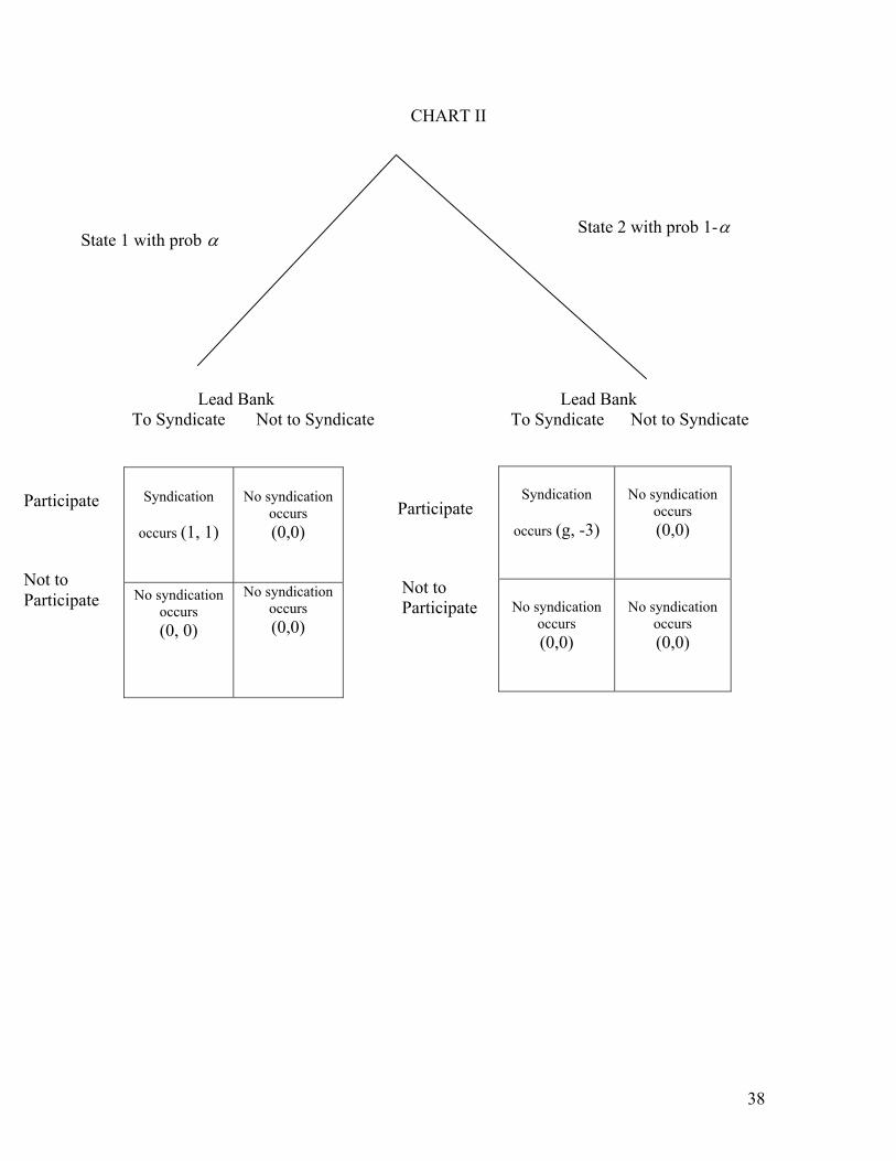
CHART II

αState 2 with prob 1-α

State 1 with prob

Lead Bank Lead Bank To Syndicate Not to Syndicate To Syndicate Not to Syndicate

Syndication

occurs (g, -3)

No syndication occurs (0,0)

No syndication No syndication

Syndication

occurs (1, 1)

No syndication occurs (0,0)

No syndication occurs (0, 0)

No syndication occurs (0,0)

Not to Participate

ParticipateParticipate

Not to Participate

occurs (0,0)

occurs (0,0)

38

CHART III

Lead Bank

Syndicate Not to Syndicate

No Syndication

Occurs (N-E)

No Syndication

Occurs (N-E)

No Syndication

Occurs (N-E)

Participate Participant agent

Not Participate

\

39

CHART IV

Lead Bank

Syndicate Not to Syndicate

Syndication Occur (N-E) (1,1)

Participate

Participant agent

Not Participate

40

Table I. Descriptive Statistics for the Sample

Variable Sample Size

Full Sample

Syndicated Loan

Non-syndicated Loan

Panel A: Descriptive statistics for discrete variables Secured Secured 12356(87.14%) 5854(82.75%) 6502(91.50%) Not-secured 1824(12.86%) 1220(17.25%) 604(8.50%) Bank Bank 12110(85.40%) 6284(88.83%) 5826(81.99%) Non-bank 2070(14.60%) 790(11.17%) 1280(18.01%) Pfprice With Performance Pricing

1145(8.07%) 627(8.86%) 518(7.29%)

Without Performance Pricing

13035(91.93%) 6447(91.14%) 6588(92.71%)

Bond Rating With Bond Rating 3577(25.23%) 2885(40.78%) 692(9.74%) Without Bond Rating 10603(74.77%) 4189(59.22%) 6414(90.26%) Ticker With Ticker 7837(55.27%) 4022(56.86%) 3815(53.69%) Without Ticker 6343(44.73%) 3052(43.14%) 3291(46.31%)

Panel B: Descriptive statistics for continuous variables mean/median

(min /max)

mean/median (min /max)

mean/median (min /max)

Maturity 14180 41.89/36 (0/408)

49.46/48 (0/366)

34.36/24 (0/408)

Facisize 14180 68.78/15 (0.005/8600)

129.69/50 (0.18/8600)

8.14/5 (0.005/1000)

Note. SECURED is a dummy equal to one if the loan is collateralized and zero otherwise; BANK is a dummy equal to one if the managing agent has a bank charter and zero otherwise; Pfprice is a dummy that equals to 1 if there is performance pricing and 0 otherwise; BONDRATE is a dummy equal to one if the borrower has a senior, unsecured debt rating and zero otherwise; TICKER is a dummy equal to one if the borrower is listed on the NYSE, AMEX or NASDAQ and zero otherwise; MATURITY is the maturity of the loan (in months); FACSIZE is the million dollar value size of the loan facility; Of the 14180 loan transactions in the sample of bank and non-bank facilities over the period of 1987-1999, 7074 (50%) are syndicated.

41

Table II. Correlation of Parameter Estimates

Panel A: For non-syndicated and syndicated loan transactions over the period 1987-1999

Bondrate Secured Bank Maturity Facsize TOTAL Pfprice

Bondrate 1 . 0 0 0 0 0

Secured -0.13672 1.00000

Bank 0 . 0 7 9 6 4 -0.12484 1.00000

Maturity 0 . 1 2 7 1 4 0.04477 -0.04760 1 . 0 0 0 0 0

Facsize 0 . 2 2 1 6 1 -0.15622 0.06118 0 . 0 7 5 0 4 1.00000

Pfprice 0.03586 -0.02993 0.01330 -0.00261 -0.00043 1.00000

Panel B: For syndicated loan transactions over the period 1987-1999 Bondrate 1 . 0 0 0 0 0

Secured -0.14531 1.00000

Bank 0 . 1 0 4 7 9 -0.14407 1.00000

Maturity 0 . 1 4 1 3 5 0.05718 -0.09405 1 . 0 0 0 0 0

Facsize 0 . 3 1 4 5 5 -0.14453 0.05725 0 . 1 0 1 1 7 1.00000

TOTAL 0 . 1 6 7 6 0 -0.16166 0.14110 -0.01110 0.14786 1.00000

Pfprice 0 . 0 2 9 4 0 -0.00084 0.03352 0 . 0 1 4 2 5 -0.00800 0.08063 1.00000

42

Table III. Descriptive Statistics for the ZCHAG Sample

Variable Sample Size

Full Sample

“active” Group

“drop-out” Group

Panel A: Descriptive statistics for discrete variables Bank Bank 1794(90.51) 857(92.25) 117(84.17) Non-bank 188(9.49) 72(7.75) 22(15.83) Bond Rating With Bond Rating 649(32.74) 483(51.99) 47(33.81) Without Bond Rating 1333(67.26) 446(48.01) 92(66.19) Pfprice With Performance Pricing

149(7.52) 87(9.36) 5(3.60)

Without Performance Pricing

1833(92.48) 842(90.64) 134(96.40)

Secured Secured 1572(79.31) 697(75.03) 120(86.33) Not-secured 410(20.69) 232(24.97) 19(13.67)

Panel B: Descriptive statistics for continuous variables mean/median

(min /max)

mean/median (min /max)

mean/median (min /max)

Facisize 1982 75.03/17.50 (0.05/5000)

134.33/60 (0.45/5000)

100.88/30 (1/2100)

Maturity 1982 42.38/36 (1/366)

48.82/46 (3/366)

47.30/47 (2/108)

TOTAL 1100 4.88/2 (-4/45)

5.46/2 (-4/45)

1.5179856/1 (-1/13)

ZCHAG 1982 0.71/-0.001 (-28.69/647.05)

0.02/-0.01 (-28.69/31.45)

0.46/0.03 (-2.2/18.2)

Note. SECURED is a dummy equal to one if the loan is collateralized and zero otherwise; BANK is a dummy equal to one if the managing agent has a bank charter and zero otherwise; Pfprice is a dummy that equals to 1 if there is the performance pricing and 0 otherwise; BONDRATE is a dummy equal to one if the borrower has a senior, unsecured debt rating and zero otherwise; TICKER is a dummy equal to one if the borrower is listed on the NYSE, AMEX or NASDAQ and zero otherwise; MATURITY is the maturity of the loan (in months); FACSIZE is the million dollar value size of the loan facility; TOTAL is the number of repeat transactions conducted with the lead bank syndicating “good” loans in the presample period with unchanged or improved Z score of the borrower minus the number of repeat transactions conducted with the lead bank syndicating “bad” loans with deteriorated Z score of the borrower. Of the 1982 loan transactions in the ZSCRORECHAG sample, 1100 (55%) are syndicated loans. The “active group” contains 929 loans. The “drop-out” group” contains 139 loans.

43

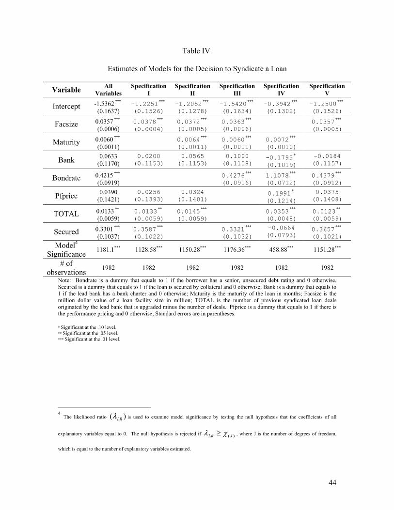
Table IV.

Estimates of Models for the Decision to Syndicate a Loan

Variable All Variables

Specification I

Specification II

Specification III

Specification IV

Specification V

Intercept -1.5362 ∗ ∗∗

(0.1637) -1.2251 ∗ ∗∗

(0.1526) -1.2052 ∗ ∗∗

(0.1278) -1.5420 ∗∗∗

(0.1634) -0.3942 ∗ ∗∗

(0.1302) -1.2500 ∗ ∗∗

(0.1526)

Facsize 0.0357 ∗∗∗

(0.0006) 0.0378 ∗ ∗∗

(0.0004) 0.0372 ∗ ∗∗

(0.0005) 0.0363 ∗∗∗

(0.0006) 0.0357 ∗ ∗∗

(0.0005)

Maturity 0.0060 ∗∗∗

(0.0011) 0.0064 ∗ ∗∗

(0.0011) 0.0060 ∗∗∗

(0.0011) 0.0072 ∗ ∗∗

(0.0010)

Bank 0.0633 (0.1170)

0.0200 (0.1153)

0.0565 (0.1153)

0.1000 (0.1158)

-0.1795 ∗ (0.1019)

-0.0184 (0.1157)

Bondrate 0.4215 ∗∗∗

(0.0919) 0.4276 ∗∗∗

(0.0916) 1.1078 ∗ ∗∗

(0.0712) 0.4379 ∗ ∗∗

(0.0912)

Pfprice 0.0390 (0.1421)

0.0256 (0.1393)

0.0324 (0.1401) 0.1991 ∗

(0.1214) 0.0375 (0.1408)

TOTAL 0.0133 ∗ ∗

(0.0059) 0.0133 ∗∗

(0.0059) 0.0145 ∗ ∗∗

(0.0059) 0.0353 ∗ ∗∗

(0.0048) 0.0123 ∗∗

(0.0059)

Secured 0.3301 ∗∗∗

(0.1037) 0.3587 ∗ ∗∗

(0.1022) 0.3321 ∗∗∗

(0.1032) -0.0664 (0.0793)

0.3657 ∗ ∗∗

(0.1021) Model4

Significance 1181.1*** 1128.58*** 1150.28*** 1176.36*** 458.88*** 1151.28***

# of observations 1982 1982 1982 1982 1982 1982

Note: Bondrate is a dummy that equals to 1 if the borrower has a senior, unsecured debt rating and 0 otherwise. Secured is a dummy that equals to 1 if the loan is secured by collateral and 0 otherwise; Bank is a dummy that equals to 1 if the lead bank has a bank charter and 0 otherwise; Maturity is the maturity of the loan in months; Facsize is the million dollar value of a loan facility size in million; TOTAL is the number of previous syndicated loan deals originated by the lead bank that is upgraded minus the number of deals. Pfprice is a dummy that equals to 1 if there is the performance pricing and 0 otherwise; Standard errors are in parentheses. * Significant at the .10 level. ** Significant at the .05 level. *** Significant at the .01 level.

4 The likelihood ratio )( LRλ is used to examine model significance by testing the null hypothesis that the coefficients of all

explanatory variables equal to 0. The null hypothesis is rejected if )( JLR χλ ≥ , where J is the number of degrees of freedom,

which is equal to the number of explanatory variables estimated.

44

Table V

Estimates of the Percentage of Syndicated of a loan

For “active” lead banks

Variable All Variable

Specification I

Specification II

Specification III

Specification IV

Specification V

Intercept 1.1634***

(0.0657) 1.1864*** (0.0573)

0.8888*** (0.0308)

1.1747*** (0.0656)

1.1942*** (0.0573)

1.1671*** (0.0657)

Facsize 0.00003

(0.00005) 0.00003 (0.00004)

0.00003 (0.00005)

0.00006 (0.00004)

0.00005 (0.00004)

0.00003 (0.00005)

Maturity 0.0006 (0.0005)

0.0007 (0.0005) 0.0007

(0.0005) 0.0007 (0.0005)

0.0006 (0.0005)

Bank -

0.3218***

(0.0590) -0.3272***

(0.0584) -0.3018***

(0.0585) -0.3068*** (0.0578)

-0.3200*** (0.0590)

Bondrate 0.0644**

(0.0282) 0.0633** (0.0282)

0.0420 (0.0282) 0.0664**

(0.0282)

Pfprice 0.0728

(0.0471) 0.0734 (0.0471)

0.0665 (0.0478)

0.0776* (0.0473)

0.0781* (0.0473)

Secured 0.0241

(0.0312) 0.0496 (0.0314)

0.0204 (0.0313) 0.0250

(0.0313) ZCHAG 0.0132**

(0.0061) 0.0134** (0.0061)

0.0113** (0.0061)

0.0128** (0.0061)

0.0131** (0.0061)

0.0133** (0.0061)

Model Significance5 43.91*** 42.72*** 10.96* 38.1*** 37.7*** 40.9***

# of observations 929 929 929 929 929 929

Note: Truncated (from above at 100%) regression estimates of the percentage of a loan being syndicated. Facsize is a million dollar value of a loan facility size (in million); Maturity is the maturity of the loan (in months); Bank is a dummy that equals to 1 if the managing agent has a bank charter and 0 otherwise; Bondrate is the variable equals to 1 if there is any senior debt rating for this borrower; Pfprice is a dummy that equals to 1 if there is the performance pricing and 0 otherwise; Secured equals to 1 if the loan is secured and 0 otherwise; ZCHAG is the Z score change one year after the facility is closed. * Significant at the .10 level. ** Significant at the .05 level. *** Significant at the .01 level.

5 The likelihood ratio )( LRλ is used to examine model significance by testing the null hypothesis that the coefficients of all

explanatory variables equal to 0. The null hypothesis is rejected if )( JLR χλ ≥ , where J is the number of degrees of freedom,

which is equal to the number of explanatory variables estimated.

45

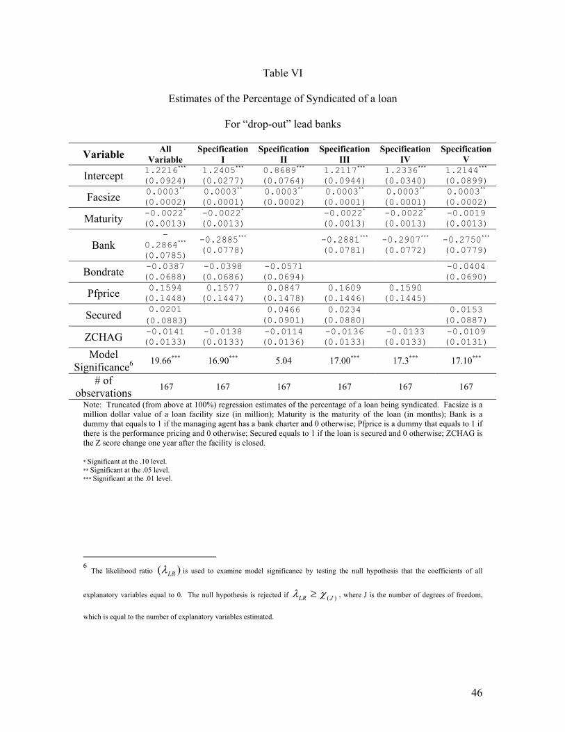
Table VI

Estimates of the Percentage of Syndicated of a loan

For “drop-out” lead banks

Variable All Variable

Specification I

Specification II

Specification III

Specification IV

Specification V

Intercept 1.2216*** (0.0924)

1.2405*** (0.0277)

0.8689*** (0.0764)

1.2117*** (0.0944)

1.2336*** (0.0340)

1.2144*** (0.0899)

Facsize 0.0003** (0.0002)

0.0003** (0.0001)

0.0003** (0.0002)

0.0003** (0.0001)

0.0003** (0.0001)

0.0003** (0.0002)

Maturity -0.0022* (0.0013)

-0.0022* (0.0013) -0.0022*

(0.0013) -0.0022* (0.0013)

-0.0019 (0.0013)

Bank -

0.2864*** (0.0785)

-0.2885*** (0.0778) -0.2881***

(0.0781) -0.2907*** (0.0772)

-0.2750*** (0.0779)

Bondrate -0.0387 (0.0688)

-0.0398 (0.0686)

-0.0571 (0.0694) -0.0404

(0.0690) Pfprice 0.1594

(0.1448) 0.1577 (0.1447)

0.0847 (0.1478)

0.1609 (0.1446)

0.1590 (0.1445)

Secured 0.0201 (0.0883) 0.0466

(0.0901) 0.0234 (0.0880) 0.0153

(0.0887) ZCHAG -0.0141

(0.0133) -0.0138 (0.0133)

-0.0114 (0.0136)

-0.0136 (0.0133)

-0.0133 (0.0133)

-0.0109 (0.0131)

Model Significance6 19.66*** 16.90*** 5.04 17.00*** 17.3*** 17.10***

# of observations 167 167 167 167 167 167

Note: Truncated (from above at 100%) regression estimates of the percentage of a loan being syndicated. Facsize is a million dollar value of a loan facility size (in million); Maturity is the maturity of the loan (in months); Bank is a dummy that equals to 1 if the managing agent has a bank charter and 0 otherwise; Pfprice is a dummy that equals to 1 if there is the performance pricing and 0 otherwise; Secured equals to 1 if the loan is secured and 0 otherwise; ZCHAG is the Z score change one year after the facility is closed. * Significant at the .10 level. ** Significant at the .05 level. *** Significant at the .01 level.

6 The likelihood ratio )( LRλ is used to examine model significance by testing the null hypothesis that the coefficients of all

explanatory variables equal to 0. The null hypothesis is rejected if )( JLR χλ ≥ , where J is the number of degrees of freedom,

which is equal to the number of explanatory variables estimated.

46

Table VII

Estimates of Models for the Decision to Syndicate a Loan for the NOTCHAG sample

Variable All Variables

Specification I

Specification II

Specification III

Specification IV

Specification V

Intercept 0.1099* (0.2134)

0.3885** (0.1870)

-0.0426 (0.1437)

0.0807 (0.2094)

0.8530*** (0.1859)

0.3712** (0.2008)

Facsize 0.0047*** (0.0006)

0.0048*** (0.0006)

0.0050*** (0.0005)

0.0049*** (0.0006) 0.0048***

(0.0006) Maturity 0.0069***

(0.0017) 0.0062*** (0.0017)

0.0069*** (0.0017)

0.0081*** (0.0016)

Bank 0.1929 (0.1293)

0.1896 (0.1289)

0.2276* (0.1275)

0.3944*** (0.1261)

0.2163* (0.1236)

0.1897 (0.1289)

Ticker 0.0749 (0.0987) 0.0761

(0.0961) 0.0670

(0.0936) 0.0229

(0.0968) Pfprice 0.3790**

(0.1657) 0.3630** (0.1644)

0.3761** (0.1653) 0.2928**

(0.1575) 0.3643** (0.1645)

TOTAL2 0.0344*** (0.0064)

0.0342*** (0.0063)

0.0339*** (0.0064) 0.0377***

(0.0060) 0.0342*** (0.0063)

Secured -0.2192 (0.1442)

-0.1198 (0.1387) -0.1410

(0.1389) -0.7091*** (0.1278)

-0.1164 (0.1395)

Model7 Significance 240.4*** 223.36*** 237.22*** 192.02*** 139.46*** 223.48***

# of observations 1452 1452 1452 1452 1452 1452

Note: Facsize is the dollar value of a loan facility in millions; Maturity is the maturity of the loan in months; Bank is a dummy that equals 1 if the lead bank has a bank charter and 0 otherwise; Ticker is a dummy equal to one if the borrower is listed on the NYSE, AMEX or NASDAQ and zero otherwise; Pfprice is a dummy that equals 1 if there is performance pricing and 0 otherwise; TOTAL2 is the number of previous syndicated loan deals the lead bank has originated where the borrower’s S&P senior debt rating is unchanged or upgraded minus the number of deals where the rating is downgraded; Secured is a dummy that equals 1 if the loan is secured by collateral and 0 otherwise. Standard errors are in parentheses.

* Significant at the .10 level. ** Significant at the .05 level. *** Significant at the .01 level.

7 The likelihood ratio )( LRλ is used to examine model significance by testing the null hypothesis that the coefficients of all

explanatory variables equal 0. The null hypothesis is rejected if )( JLR χλ ≥ , where J is the number of degrees of freedom, which

is equal to the number of explanatory variables estimated.

47

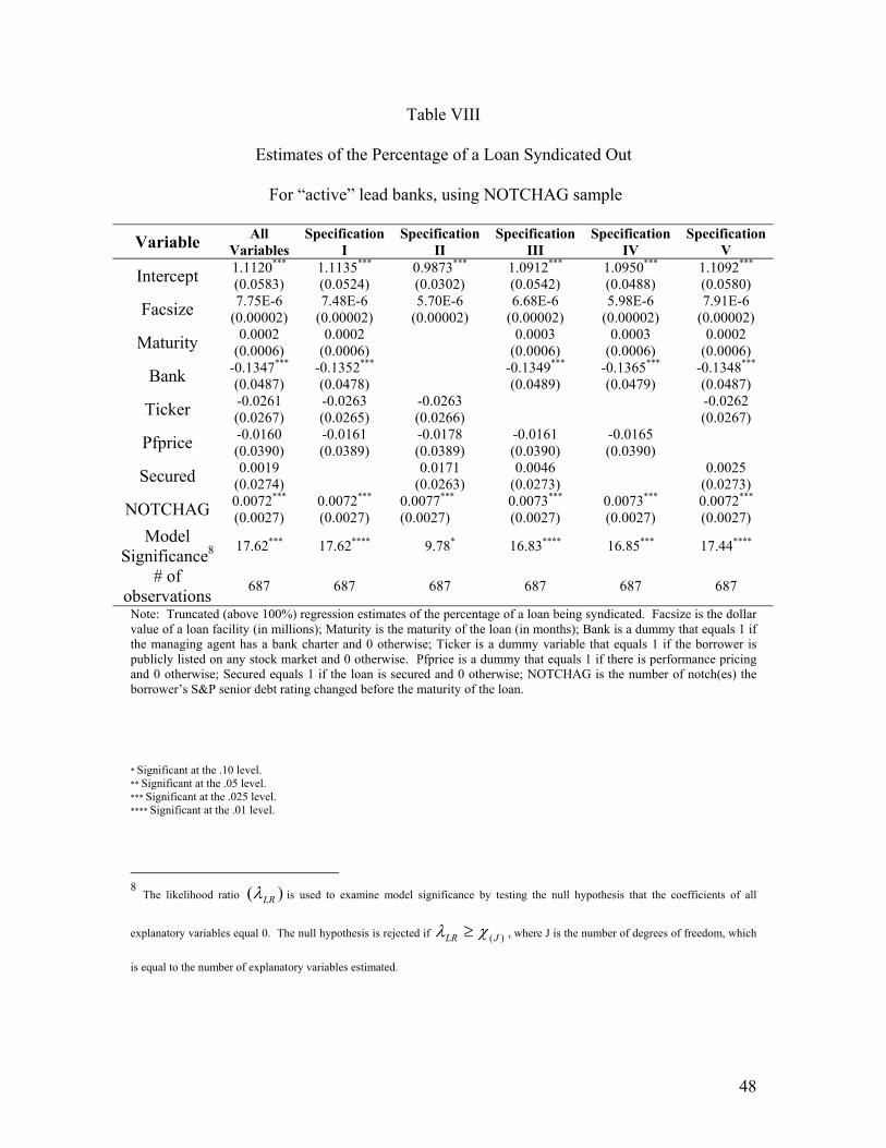
Table VIII

Estimates of the Percentage of a Loan Syndicated Out

For “active” lead banks, using NOTCHAG sample

Variable All Variables

Specification I

Specification II

Specification III

Specification IV

Specification V

Intercept 1.1120*** (0.0583)

1.1135*** (0.0524)

0.9873*** (0.0302)

1.0912*** (0.0542)

1.0950*** (0.0488)

1.1092*** (0.0580)

Facsize 7.75E-6 (0.00002)

7.48E-6 (0.00002)

5.70E-6 (0.00002)

6.68E-6 (0.00002)

5.98E-6 (0.00002)

7.91E-6 (0.00002)

Maturity 0.0002 (0.0006)

0.0002 (0.0006) 0.0003

(0.0006) 0.0003

(0.0006) 0.0002

(0.0006)

Bank -0.1347*** (0.0487)

-0.1352*** (0.0478) -0.1349***

(0.0489) -0.1365*** (0.0479)

-0.1348*** (0.0487)

Ticker -0.0261 (0.0267)

-0.0263 (0.0265)

-0.0263 (0.0266) -0.0262

(0.0267)

Pfprice -0.0160 (0.0390)

-0.0161 (0.0389)

-0.0178 (0.0389)

-0.0161 (0.0390)

-0.0165 (0.0390)

Secured 0.0019 (0.0274) 0.0171

(0.0263) 0.0046

(0.0273) 0.0025 (0.0273)

NOTCHAG 0.0072*** (0.0027)

0.0072*** (0.0027)

0.0077*** (0.0027)

0.0073*** (0.0027)

0.0073*** (0.0027)

0.0072*** (0.0027)

Model Significance8 17.62*** 17.62**** 9.78* 16.83**** 16.85*** 17.44****

# of observations 687 687 687 687 687 687

Note: Truncated (above 100%) regression estimates of the percentage of a loan being syndicated. Facsize is the dollar value of a loan facility (in millions); Maturity is the maturity of the loan (in months); Bank is a dummy that equals 1 if the managing agent has a bank charter and 0 otherwise; Ticker is a dummy variable that equals 1 if the borrower is publicly listed on any stock market and 0 otherwise. Pfprice is a dummy that equals 1 if there is performance pricing and 0 otherwise; Secured equals 1 if the loan is secured and 0 otherwise; NOTCHAG is the number of notch(es) the borrower’s S&P senior debt rating changed before the maturity of the loan. * Significant at the .10 level. ** Significant at the .05 level. *** Significant at the .025 level. **** Significant at the .01 level.

8 The likelihood ratio )( LRλ is used to examine model significance by testing the null hypothesis that the coefficients of all

explanatory variables equal 0. The null hypothesis is rejected if )(JLR χλ ≥ , where J is the number of degrees of freedom, which

is equal to the number of explanatory variables estimated.

48

Table IX

Estimates of the Percentage of a Loan Syndicated Out

For “drop-out” lead banks, using NOTCHAG sample

Variable All Variables

Specification I

Specification II

Specification III

Specification IV

Specification V

Intercept 1.2648 (0.3061)

1.4334*** (0.2437)

0.7536*** (0.2130)

1.5285*** (0.2614)

1.6019*** (0.2142)

1.2610*** (0.3057)

Facsize 0.0003 (0.0003)

0.0002 (0.0002)

0.0003 (0.0003)

0.0002 (0.0004)

0.0002 (0.0003)

0.0003 (0.0003)

Maturity -0.0063*** (0.0020)

-0.0062*** (0.0020) -0.0065***

(0.0021) -0.0065*** (0.0021)

-0.0062*** (0.0020)

Bank -0.2384 (0.2129)

-0.2475 (0.2152) -0.3105

(0.2154) -0.3112 (0.2163)

-0.2414 (0.2109)

Ticker 0.1753 (0.1196)

0.1435 (0.1149)

0.2301* (0.1264) 0.1753

(0.1196) Pfprice -0.0231

(0.1484) -0.0262 (0.1486)

0.0068 (0.1617)

-0.0209 (0.1533)

-0.0226 (0.1531)

Secured 0.1478 (0.1657) 0.1466

(0.1717) 0.0786

(0.1638) 0.1485 (0.1654)

NOTCHAG -0.0012 (0.0137)

-0.0038 (0.0134)

0.0072 (0.0143)

-0.00007 (0.0142)

-0.0017 (0.0138)

-0.0013 (0.0136)

Model Significance9 14.98*** 14.22*** 4.56 12.94** 12.85*** 14.96***

# of observations 62 62 62 62 62 62

Note: Truncated (above 100%) regression estimates of the percentage of a loan syndicated. Facsize is the dollar value of a loan facility (in millions); Maturity is the maturity of the loan (in months); Bank is a dummy that equals 1 if the managing agent has a bank charter and 0 otherwise; Ticker is a dummy variable that equals 1 if the borrower is publicly listed on any stock market and 0 otherwise. Pfprice is a dummy variable that equals to 1 if there is the performance pricing and 0 otherwise; Secured equals 1 if the loan is secured and 0 otherwise; NOTCHAG is the number of notch(es) the borrower’s S&P senior debt rating changed before the maturity of the loan. * Significant at the .10 level. ** Significant at the .05 level. *** Significant at the .025 level. **** Significant at the .01 level.

9 The likelihood ratio )( LRλ is used to examine model significance by testing the null hypothesis that the coefficients of all

explanatory variables equal 0. The null hypothesis is rejected if )( JLR χλ ≥ , where J is the number of degrees of freedom, which

is equal to the number of explanatory variables estimated.

49