Synchronization of spin trasnsfer nano-oscillators
235
HAL Id: tel-01126902 https://tel.archives-ouvertes.fr/tel-01126902 Submitted on 6 Mar 2015 HAL is a multi-disciplinary open access archive for the deposit and dissemination of sci- entific research documents, whether they are pub- lished or not. The documents may come from teaching and research institutions in France or abroad, or from public or private research centers. L’archive ouverte pluridisciplinaire HAL, est destinée au dépôt et à la diffusion de documents scientifiques de niveau recherche, publiés ou non, émanant des établissements d’enseignement et de recherche français ou étrangers, des laboratoires publics ou privés. Synchronization of spin trasnsfer nano-oscillators Abbass Hamadeh To cite this version: Abbass Hamadeh. Synchronization of spin trasnsfer nano-oscillators. Materials Science [cond- mat.mtrl-sci]. Université Paris Sud - Paris XI, 2014. English. NNT: 2014PA112262. tel-01126902
Transcript of Synchronization of spin trasnsfer nano-oscillators

HAL Id: tel-01126902https://tel.archives-ouvertes.fr/tel-01126902
Submitted on 6 Mar 2015
HAL is a multi-disciplinary open accessarchive for the deposit and dissemination of sci-entific research documents, whether they are pub-lished or not. The documents may come fromteaching and research institutions in France orabroad, or from public or private research centers.
L’archive ouverte pluridisciplinaire HAL, estdestinée au dépôt et à la diffusion de documentsscientifiques de niveau recherche, publiés ou non,émanant des établissements d’enseignement et derecherche français ou étrangers, des laboratoirespublics ou privés.
Synchronization of spin trasnsfer nano-oscillatorsAbbass Hamadeh
To cite this version:Abbass Hamadeh. Synchronization of spin trasnsfer nano-oscillators. Materials Science [cond-mat.mtrl-sci]. Université Paris Sud - Paris XI, 2014. English. NNT : 2014PA112262. tel-01126902
UNIVERSITE DE PARIS-SUD
UFR Scientifique d’OrsayEcole Doctorale de Physique en Ile-de-France (ED-564)
CEA SACLAY
These de Doctorat
presentee pour obtenirle grade de Docteur en sciences
de l’UNIVERSITE PARIS XI, ORSAY
Specialite:Physique
par
Abbass Hamadeh
Synchronization of spin transfer nano-oscillators
Soutenue le 3 Octobre 2014 au CEA Saclay devant le jury compose de :
Rapporteurs Mme. Ursula EbelsM. Stephane Mangin
Examinateurs M. Andre ThiavilleM. Andrei SlavinM. Vincent Cros
Directeur de these M. Olivier KleinCo-encadrant M. Gregoire de Loubens

Synchronization of spin transfer nano-oscillators
Abstract
Spin transfer nano-oscillators (STNOs) are nanoscale devices capable of generating highfrequency microwave signals through spin momentum transfer. Although they offerdecisive advantages compared to existing technology (spectral agility, integrability, etc.),their emitted power and spectral purity are quite poor. In view of their applications, apromising strategy to improve the coherence and increase the emitted microwave powerof these devices is to mutually synchronize several of them. A first step is to understandthe synchronization of a single STNO to an external source. For this, we have studieda circular nanopillar of diameter 200 nm patterned from a Cu60∣Py15∣ Cu10∣Py4∣Au25stack, where thicknesses are in nm. In the saturated state (bias magnetic field > 0.8 T),we have identified the auto-oscillating mode and its coupling to an external source byusing a magnetic resonance force microscope (MRFM). Only the uniform microwavefield applied perpendicularly to the bias field is efficient to synchronize the STNObecause it shares the spatial symmetry of the auto-oscillation mode, in contrast to themicrowave current passing through the device. The same sample was then studiedunder low perpendicular magnetic field, with the two magnetic layers in the vortexstate. In this case, it is possible to excite a highly coherent mode (F /∆F > 15000) witha linewidth below 100 kHz. By analyzing the harmonic content of the spectrum, wehave determined that the non-linear amplitude-phase coupling of the excited modeis almost vanishing, which explains the high spectral purity observed. Moreover, theoscillation frequency can still be widely tuned thanks to the Oersted field created by thedc current. We have also shown that the synchronization of this mode to a microwavefield source is very robust, the generation linewidth decreasing by more than five ordersof magnitude compared to the autonomous regime. From these findings we concludethat the magneto-dipolar interaction is promising to achieve mutual coupling of vortexbased STNOs, the dipolar field from a neighboring oscillator playing the role of themicrowave source. We have thus experimentally measured a system composed of twoSTNOs laterally separated by 100 nm. By varying the different configurations of vortexpolarities, we have observed the mutual synchronization of these two oscillators.Keywords: Magnetism; spintronics; microwave; oscillators; synchronization MRFM-magnetic resonance force microscopy; magnetic vortex state; dipolar coupling.


Synchronisation de nano-oscillateurs a transfert de spin
Resume
Les nano-oscillateurs a transfert de spin (STNOs) sont des dispositifs capables d’emettreune onde hyperfrequence lorsqu’ils sont pompes par un courant polarise grace aucouple de transfert de spin. Bien qu’ils offrent de nombreux avantages (agilite spec-trale, integrabilite, etc.) pour les applications, leur puissance d’emission et leur puretespectrale sont en general faibles. Une strategie pour ameliorer ces proprietes est desynchroniser plusieurs oscillateurs entre eux. Une premiere etape est de comprendrela synchronisation d’un STNO unique a une source externe. Pour cela, nous avonsetudie une vanne de spin Cu60∣NiFe15∣Cu10∣NiFe4∣Au25 (epaisseurs en nm) de sectioncirculaire de 200 nm. Dans l’etat sature perpendiculaire (champ applique > 0.8 T), nousavons determine la nature du mode qui auto-oscille et son couplage a une source externegrace a un microscope de force par resonance magnetique (MRFM). Seul un champmicro-onde uniforme permet de synchroniser le mode oscillant de la couche fine caril possede la bonne symetrie spatiale, au contraire du courant micro-onde traversantl’echantillon. Ce meme echantillon a ensuite ete etudie sous faible champ perpendic-ulaire, les deux couches magnetiques etant alors dans l’etat vortex. Dans ce cas, il estpossible d’exciter un mode de grande coherence (F /∆F > 15000) avec une largeur deraie inferieure a 100 kHz. En analysant le contenu harmonique du spectre, nous avonsdetermine que le couplage non-lineaire amplitude-phase du mode excite est quasi nul,ce qui explique la grande purete spectrale observee, et qu’en parallele, la frequenced’oscillation reste ajustable sur une grande gamme grace au champ d’Oersted creepar le courant injecte. De plus, la synchronisation de ce mode a une source de champmicro-onde est tres robuste, la largeur de raie mesuree diminuant de plus de cinq ordresde grandeur par rapport au regime autonome. Nous concluons de cette etude que lecouplage magneto-dipolaire entre STNOs a base de vortex est tres prometteur pourobtenir une synchronisation mutuelle, le champ dipolaire rayonne par un STNO surses voisins jouant alors le role de la source micro-onde. Nous sommes donc passes al’etape suivante, a savoir la mesure experimentale de deux STNOs similaires separeslateralement de 100 nm. En jouant sur les differentes configurations de polarites des vor-tex, nous avons reussi a observer la synchronisation mutuelle de ces deux oscillateurs.Mots-cles : Magnetisme; electronique de spin; hyperfrequence; oscillateurs; MRFM;synchronisation; MRFM-microscopie de force a resonance magnetique; etat vortexmagnetique; couplage dipolaire.


Remerciements
Enfin, le navire qui avait quitte son port il y a 3 ans, est revenu, regorgeant d’informationset de resultats inscrits dans cette these. Mon bonheur ne connaıt point de limite, mareconnaissance aussi a l’egard de toutes les personnes qui m’ont assure de leur soutienet de leur aide durant ce periple.
En premier lieu, mes remerciements s’adressent a Olivier Klein et Gregoire de Loubensqui m’ont inculque le gout et la passion de la physique que j’ai decouverte sans limiteni reserve. Je vous remercie pour avoir ete mes “pagaies”, me propulsant toujoursvers l’avant. Je vous remercie pour avoir ete “la boussole” qui me montrait le chemin.Vous m’avez permis de grandir en amour et en passion pour la physique. J’aimeraisegalement vous dire a quel point j’ai apprecie vos grandes disponibilites et vos respectssans faille des delais serres de relecture ma these que je vous ai adresses. Enfin, j’ai eteextremement sensible a vos qualites humaines d’ecoute et de comprehension tout aulong de ce travail de these.
Mes remerciements vont egalement a Vladimir Naletov. Son aide et son soutien aura etesans faille durant une grande partie de ma these, et j’ai grandement apprecie sa reactiviteet sa gentillesse.
Je remercie chaleureusement Ursula Ebels et Stephane Mangin d’avoir accepte d’etrerapporteurs de ce manuscrit, ainsi les menbres du jury de these Andrei Slavin, AndreThiaville et Vincent Cros pour leurs remarques.
Ce travail de these a ete effectue au SPEC au sein de Laboratoire Nano-magnetismeet Oxydes (LNO). Je remercie tous les personnes de SPEC qui ont attribue dune faconou dune autre a ce travail, en particulier Claude Fermon de m’avoir accueilli dansleur laboratoire. Je remercie egalement Michel Viret pour toutes les discussions et lapreparation des contact de echantillons de disques de YIG. Grand merci.
Evidemment ces annees passees au sein de LNO n’auraient pas ete sans la gentillessede l’ensemble des membres du Groupe. Je remercie sincerement tous les permanentsdu groupes . Je souhaite remercier aussi mes colleges de LNO (Thesards, Post-docs,Ingenieurs, Stagieres ..), avec lesquels j’ai partage de bons moments, Merci donc a,Christian, Benjamin, Pierre-andre, Camille, Jean-Yves, Laure, Quentin, Amala, Elodie,Aurelie, Olivier, Paolo, Soraya, Hugo, Remy, Damien, Ruben, Vincent ... pour leursoutien inconditionnel aussi je les remercie pour leur sympathie. Je noublie pas de
7

– 8 –
remercier mes amis, de SPEC ainsi que en dehors du Laboratoire, qui mont soutenudurant ces trois ans, avec eux j’ai partage de bons moments ainsi que des momentsdifficiles.
Je tiens aussi a remercier les personnes du l’unite mixte CNRS Thales avec qui j’aicollabore pour mon travail. Tout d’abord Vincent Cros pour les fructueuses discussionsque nous avons eues. Mes remerciements vont egalement a Julie Grollier, Madjid Anane,Nicolas Locatteli, Romain Lebrun (bon courage pour la suite), Eva Grimaldy, ALexJenkis et Olivier Dallivykelly.
Je ne saurai oublier de remercier tous mes professeurs qui mont appris de leursavoir faire, en particulier Monsieur Jean-Jacques Greffet, responsable de Master 2nanophysique et Monsieur Jerome Leygnier responsable de Master 1 physique fonda-mentale pour les differents conseils. Je ne les oublierai jamais.
Enfin ma reconnaissance va a ceux qui ont plus particulierement assure le soutien affectifde ce travail : ma famille ainsi que ma cherie.
Abbass HAMADEH
Table of Contents
Abstract 3
Resume 5
Remerciements 7
Introduction 150.1. Context . . . . . . . . . . . . . . . . . . . . . . . . . . . . . . . . . . . . . . . . . 15
0.2. Motivations . . . . . . . . . . . . . . . . . . . . . . . . . . . . . . . . . . . . . . 16
0.3. Methods . . . . . . . . . . . . . . . . . . . . . . . . . . . . . . . . . . . . . . . . 18
0.4. Outline of the manuscript . . . . . . . . . . . . . . . . . . . . . . . . . . . . . . 19
I. Background 21
1. Spin transfer nano-oscillators 231.1. Equation of motion of magnetization . . . . . . . . . . . . . . . . . . . . . . . 24
1.1.1. Conservative terms . . . . . . . . . . . . . . . . . . . . . . . . . . . . . 24
1.1.2. Non-conservative terms . . . . . . . . . . . . . . . . . . . . . . . . . . 26
1.1.3. Critical current . . . . . . . . . . . . . . . . . . . . . . . . . . . . . . . . 28
9
– 10 – Table of Contents
1.2. The vortex state . . . . . . . . . . . . . . . . . . . . . . . . . . . . . . . . . . . . 29
1.2.1. Static properties . . . . . . . . . . . . . . . . . . . . . . . . . . . . . . . 29
1.2.1.1. Vortex stability under applied magnetic field . . . . . . . 32
1.2.1.2. Vortex stability under applied DC current . . . . . . . . . 35
1.2.2. Gyrotropic mode . . . . . . . . . . . . . . . . . . . . . . . . . . . . . . 36
1.3. State-of-the-art of STNOs experimental results . . . . . . . . . . . . . . . . . 39
1.3.1. Individual STNOs . . . . . . . . . . . . . . . . . . . . . . . . . . . . . . 40
1.3.2. Phase-locking and mutual synchronization . . . . . . . . . . . . . . 43
2. Classification of spin-wave modes in magnetic nanostructures 47
2.1. General approach . . . . . . . . . . . . . . . . . . . . . . . . . . . . . . . . . . 48
2.2. Normally magnetized thin disk . . . . . . . . . . . . . . . . . . . . . . . . . . 50
2.2.1. The eigen-modes . . . . . . . . . . . . . . . . . . . . . . . . . . . . . . 50
2.2.2. Selection rules . . . . . . . . . . . . . . . . . . . . . . . . . . . . . . . . 52
2.2.3. Influence of symmetry breaking . . . . . . . . . . . . . . . . . . . . . 52
2.3. Disk in the vortex state . . . . . . . . . . . . . . . . . . . . . . . . . . . . . . . 53
2.3.1. Gyrotropic mode in the cone state . . . . . . . . . . . . . . . . . . . . 54
2.3.2. Higher order spin-wave modes . . . . . . . . . . . . . . . . . . . . . 55
2.4. Collective spin-wave modes induced by the dipolar interaction . . . . . . 58
2.4.1. Strength of the dynamic magneto-dipolar coupling . . . . . . . . . 58
2.4.2. Coupled equations of motion and collective dynamics . . . . . . . 59
3. Nonlinear auto-oscillator theory 63
3.1. Harmonic oscillator : introduction to useful concepts . . . . . . . . . . . . 64
3.1.1. Free, damped and driven oscillator . . . . . . . . . . . . . . . . . . . 64
3.1.2. Self-sustained oscillator . . . . . . . . . . . . . . . . . . . . . . . . . . 67
3.2. Non-linear auto-oscillator model . . . . . . . . . . . . . . . . . . . . . . . . . 69
3.3. The noise in the NAO Theory . . . . . . . . . . . . . . . . . . . . . . . . . . . 72
3.3.1. Amplitude and phase fluctuations . . . . . . . . . . . . . . . . . . . . 72
3.3.2. Power generated by a STNO . . . . . . . . . . . . . . . . . . . . . . . 74
3.3.3. Generation linewidth of an STNO . . . . . . . . . . . . . . . . . . . . 75
3.4. Phase-locking and mutual synchronization . . . . . . . . . . . . . . . . . . . 78
3.5. Multi-mode oscillator . . . . . . . . . . . . . . . . . . . . . . . . . . . . . . . . 82
Abbass HAMADEH

Table of Contents – 11 –
II. Experimental setup and samples 85
4. High frequency transport and MRFM 874.1. Transport measurement . . . . . . . . . . . . . . . . . . . . . . . . . . . . . . . 88
4.2. Magnetic Resonance Force Microscopy . . . . . . . . . . . . . . . . . . . . . 89
4.2.1. Introdution . . . . . . . . . . . . . . . . . . . . . . . . . . . . . . . . . . 90
4.2.2. MRFM operating principles . . . . . . . . . . . . . . . . . . . . . . . . 90
4.2.3. Experimental realization . . . . . . . . . . . . . . . . . . . . . . . . . . 92
4.2.3.1. Cantilever . . . . . . . . . . . . . . . . . . . . . . . . . . . . . 95
4.2.3.2. Probe magnet . . . . . . . . . . . . . . . . . . . . . . . . . . . 96
4.2.4. Experimental precision . . . . . . . . . . . . . . . . . . . . . . . . . . . 97
4.2.4.1. Tip stray field . . . . . . . . . . . . . . . . . . . . . . . . . . . 97
4.2.4.2. Calibration of ∆Mz . . . . . . . . . . . . . . . . . . . . . . . 98
5. Studied samples 1015.1. Nano-pillar structure and sample design . . . . . . . . . . . . . . . . . . . . 102
5.1.1. The lithographically patterned nanostructure . . . . . . . . . . . . . 102
5.1.2. The different samples . . . . . . . . . . . . . . . . . . . . . . . . . . . . 104
5.2. The microwave circuit: design and calibration . . . . . . . . . . . . . . . . . 105
5.2.1. Modulation of the microwave source . . . . . . . . . . . . . . . . . . 105
5.2.2. Calibration of microwave setup . . . . . . . . . . . . . . . . . . . . . 107
5.2.2.1. Calibration of rf field . . . . . . . . . . . . . . . . . . . . . . 107
5.2.2.2. Calibration of rf current . . . . . . . . . . . . . . . . . . . . 107
5.3. The magnetic properties of the sample . . . . . . . . . . . . . . . . . . . . . . 108
5.4. DC and high frequency characterization . . . . . . . . . . . . . . . . . . . . . 108
5.4.1. DC characterization . . . . . . . . . . . . . . . . . . . . . . . . . . . . . 108
5.4.2. RF characterization . . . . . . . . . . . . . . . . . . . . . . . . . . . . . 109
5.5. Eigen-modes in the saturated state . . . . . . . . . . . . . . . . . . . . . . . . 110
III. Experimental results 113
6. Nanopillar in the normally magnetized state 1156.1. Perfect axial symmetry . . . . . . . . . . . . . . . . . . . . . . . . . . . . . . . 116
6.1.1. Autonomous regime . . . . . . . . . . . . . . . . . . . . . . . . . . . . 117
6.1.1.1. Phase diagram of autonomous dynamics . . . . . . . . . . 117
6.1.1.2. Identification of the auto-oscillating mode . . . . . . . . . 121
Synchronization of spin trasnsfer nano-oscillators

– 12 – Table of Contents
6.1.2. Forced regime . . . . . . . . . . . . . . . . . . . . . . . . . . . . . . . . 1246.2. Broken axial symmetry . . . . . . . . . . . . . . . . . . . . . . . . . . . . . . . 127
6.2.1. Autonomous regime . . . . . . . . . . . . . . . . . . . . . . . . . . . . 1286.2.2. Forced regime . . . . . . . . . . . . . . . . . . . . . . . . . . . . . . . . 1336.2.3. Synchronization: SATM data vs. MRFM data . . . . . . . . . . . . . 138
6.3. Spin transfer dynamics at large applied current . . . . . . . . . . . . . . . . 1396.3.1. Excitation of coupled dynamics modes . . . . . . . . . . . . . . . . . 1396.3.2. Characterization of coupled dynamics modes . . . . . . . . . . . . . 140
6.4. Conclusion . . . . . . . . . . . . . . . . . . . . . . . . . . . . . . . . . . . . . . . 143
7. Nano-pillar in the double-vortex state 1457.1. Introduction . . . . . . . . . . . . . . . . . . . . . . . . . . . . . . . . . . . . . . 1467.2. Autonomous regime: analysis of linewidth and tunability . . . . . . . . . 148
7.2.1. High frequency properties . . . . . . . . . . . . . . . . . . . . . . . . . 1497.2.2. Origin of narrow linewidth . . . . . . . . . . . . . . . . . . . . . . . . 1507.2.3. Origin of tunability . . . . . . . . . . . . . . . . . . . . . . . . . . . . . 1527.2.4. Influence of other modes . . . . . . . . . . . . . . . . . . . . . . . . . . 1537.2.5. Self parametric excitation . . . . . . . . . . . . . . . . . . . . . . . . . 155
7.2.5.1. Spectral measurement . . . . . . . . . . . . . . . . . . . . . 1567.2.5.2. Threshold and bandwidth of self-parametric excitation . 159
7.3. Forced regime . . . . . . . . . . . . . . . . . . . . . . . . . . . . . . . . . . . . . 1617.3.1. Synchronization at fundamental frequency . . . . . . . . . . . . . . 1627.3.2. Fractional synchronization . . . . . . . . . . . . . . . . . . . . . . . . 1637.3.3. Perfect and robust synchronization . . . . . . . . . . . . . . . . . . . 1647.3.4. Role of noise in phase-locking phenomena . . . . . . . . . . . . . . 167
7.4. Conclusion . . . . . . . . . . . . . . . . . . . . . . . . . . . . . . . . . . . . . . . 169
8. Dipolar coupling between adjacent STNOs 1718.1. Introduction to mutual synchronization . . . . . . . . . . . . . . . . . . . . . 1728.2. Device structure and characterization . . . . . . . . . . . . . . . . . . . . . . 173
8.2.1. Device structure . . . . . . . . . . . . . . . . . . . . . . . . . . . . . . . 1738.2.2. DC transport characterization of double STNOs . . . . . . . . . . . 173
8.3. Advantage of vortex-state over saturated state . . . . . . . . . . . . . . . . . 1768.4. Experimental results on a pairs of STNOs in the vortex states . . . . . . . 176
8.4.1. Synchronization versus applied field . . . . . . . . . . . . . . . . . . 1788.4.2. Synchronization versus DC current . . . . . . . . . . . . . . . . . . . 1818.4.3. Discussion . . . . . . . . . . . . . . . . . . . . . . . . . . . . . . . . . . . 183
Abbass HAMADEH
Table of Contents – 13 –
8.5. Theoretical analysis and numerical simulations . . . . . . . . . . . . . . . . 1838.5.1. Synchronization efficiency: P vs. AP polarities . . . . . . . . . . . . 1838.5.2. Theoretical modeling . . . . . . . . . . . . . . . . . . . . . . . . . . . . 1858.5.3. Discussion . . . . . . . . . . . . . . . . . . . . . . . . . . . . . . . . . . . 188
8.6. Conclusion . . . . . . . . . . . . . . . . . . . . . . . . . . . . . . . . . . . . . . . 189
Conclusion and perspectives 191
Appendices 195
A. Differential phase diagrams 197
B. STNO power at large positive current 199
C. Strongly mutually coupled oscillators 201
D. Pair STNOs in the saturated state 205
E. Resume substantiel en Francais 207
Synchronization of spin trasnsfer nano-oscillators


Introduction
0.1. Context
Technological progress in the fabrication of hybrid nanostructures incorporating mag-netic metals has allowed the emergence of spintronics. This field of research capitalizeson the spin degree of freedom of electron [ 1]: spin currents are generated and manipu-lated at the nanometer scale in order to achieve novel functionalities.
An elementary device of spintronics consists of two magnetic layers separated by anormal layer. It exhibits the well-known giant magnetoresistance (GMR) effect [2, 3],that is, its resistance depends on the relative angle of
Ð→M between the magnetic layers.
Nowadays, this useful property is extensively used in magnetic sensors [4, 5]. Theconverse effect is that a direct current can transfer spin angular momentum between twomagnetic layers separated by either a normal metal or a thin insulating layer [6, 7]. Moregenerally, a spin current exerts on a ferromagnetic material a spin transfer torque, thatcan compensate the damping and lead to the destabilization of the magnetic moment [8].Practical applications are the possibility to control the digital information in magneticrandom access memories (MRAMs) [9, 10] or to produce high-frequency signals inspin-transfer nano-oscillators (STNOs) [11, 12].
Owing to their tunability, agility, compactness, and integrability, STNOs are promisingcandidates for various high frequency applications such as frequency generation [13, 14],
15

– 16 – Introduction
frequency detection [15, 16], signal processing [17, 18] and dynamic recording [19, 20, 21].As far as microwave applications are concerned, spectral purity and tuning sensitivityare two key characteristics for STNOs. A particularity of such devices compared to otheroscillators is their strong nonlinear properties, which are inherited from the equationof motion of magnetization [22]. On one hand, they confer interesting properties toSTNOs, as for instance their large frequency tunability [11, 12, 13, 14]. On the otherhand, they lead to a severe broadening of the generation linewidth [23]: due to nonlinearphase-amplitude coupling, the phase noise of STNOs is indeed rather large [24, 25],which is the main limiting factor to their practical applications. Hence, non-linearitiesaffect both the agility and spectral purity in a way such that both quantities cannot beoptimized independently and a compromise must be found. Moreover, STNOs beingnanoscale microwave generators, their emitted power is very tiny, typically in the rangeof pico- or nano-Watts. In that context, mutual phase-locking of several STNOs has beenproposed as means to reduce the phase noise and increase the power generated of suchoscillators [26, 22]. To date, there are a few experimental realizations of this idea, basedon specific systems with 2 ≤ N ≤ 4 mutually-synchronized STNOs [27, 28, 29, 30]. Themain limitations in developing large arrays of synchronized STNOs are: the dispersionof dynamical properties due to uncertainties in the fabrication process, the strength ofthe dynamical coupling, and its symmetry, which might prevent synchronization oflarge arrays. For example, for the same reason why the dipolar coupling alone cannotbe responsible for a spontaneous magnetization (ferromagnetism), one cannot build aclosed-packed 3D array of oscillators synchronized through the dipolar coupling.
0.2. Motivations
This thesis work has been motivated by understanding better the microwave propertiesof STNOs, a prerequisite if one wants to optimize their performance at the level of singledevice or several mutually coupled oscillators. To achieve this goal, a spectroscopicpoint of view has been adopted, because the knowledge of the spectrum of spin-waveeigenmodes in hybrid magnetic nanostructures, namely of their symmetries, energies,relaxation rates, and nonlinear properties, is crucial in many aspects. On one side,the spin-wave energies, relaxation rates, and nonlinear properties determine at whichfrequencies and with which spectral linewidth STNOs can emit [22]. On the other side,the spatial symmetry of the modes gives a fundamental insight about their selection
Abbass HAMADEH

0.2. Motivations – 17 –
rules (how they couple to external sources) and about the mutual coupling mechanismsthat might exist intra- or inter-STNOs.
The spin-wave eigenmodes can be considered as a fingerprint of a magnetic nanostruc-ture and are deeply linked to its ground state [31, 32]. Moreover, due to interactionsbetween the different magnetic layers in a STNO (e.g., the dipolar interaction), theseeigenmodes often have a collective character, i.e., they involve several layers in the stack.A few years ago, it was experimentally shown that spin transfer torque could excitethe gyrotropic mode of a magnetic vortex [33], which is the lowest energy mode of thistopological ground state [34]. The remarkably narrow generation linewidths (about1 MHz or less) and the large output power in the case of magnetic tunnel junctions(MTJs) demonstrated by UMR CNRS/Thales in collaboration with AIST (Japan) [35],are extremely promising for applications1. In parallel, it was realized in the Spintec labof CEA that the excitation of coupled modes in uniformly magnetized standard MTJscould improve the linewidth by up to one order of magnitude [38, 39]. Shortly before thebeginning of this thesis, my lab in CEA/SPEC and the UMR CNRS/Thales combinedthese two ideas to minimize even more the auto-oscillation linewidth. By operatinga STNO based on two coupled vortices in a spin-valve nanopillars, they obtained arecord low linewidth of ∆f = 46 kHz (for a generated frequency f ≃ 780 MHz, i.e.,f/∆f ≈ 17 000) [40]. Importantly for applications, a high coherence was kept even atzero magnetic field, and a large frequency tunability on dc current (≈ 10 MHz/mA) wasmeasured.
In order to define a strategy to optimize the microwave characteristics (in particular thecoherence) of individual STNOs and to efficiently couple several STNOs together, thefollowing questions have to be addressed:
1. What is the nature of the auto-oscillating eigenmode(s) in a STNO?
2. What is the influence of other modes in the system on the spectral emission?
3. What are the nonlinearities in the system? Which other properties can influencethe spectral linewidth and the tunability?
4. What is the optimal coupling mechanism to phase-lock the auto-oscillation to anexternal source?
1Recently, up to a few micro-Watts have been reported in optimized stacks having large magnetoresistanceratio and supporting large dc currents[36]. The low phase noise in vortex MTJs has also been directlymeasured and analyzed [37]
Synchronization of spin trasnsfer nano-oscillators

– 18 – Introduction
5. What is the best strategy to mutually synchronize several STNOs in a scalableway?
The goal of this thesis is to bring some insights to these different points, with a specialfocus to understand the interesting properties of vortex-based STNOs. In particular,the interplay between the different non-linearities and the limitations has been so farextensively studied in the case of uniformly magnetized state. The role of the magneticconfiguration and its influence on the non-linear properties were still an open questionat the beginning of my thesis.
0.3. Methods
To tackle these open questions, an experimental approach has been followed. Therefore,detailed high-frequency studies of well characterized STNOs have to be conducted. Ifone wants to be able to understand with sufficient accuracy their microwave properties, itis important to work with STNO samples having a simple design and high symmetry.
The work has thus been focused on a standard circular nanopillar composed of only twoferromagnetic layers having different thicknesses and separated by a normal metal layer.When magnetized by a large perpendicular magnetic field applied along its normal,the axial symmetry of this STNO allows for a simplified identification of its spin-waveeigenmodes [41]. Moreover, the same device exhibits the double vortex configuration(one vortex in each magnetic layer) with outstanding microwave properties [40]. This
sample, an archetype of STNO, is thus particularly adapted to bring useful answers tothe questions raised by the motivations of this thesis. To be consistent with our roadmap, the same STNO device, but duplicated, will be used in the studies of mutualsynchronization.
An originality of this work is its spectroscopic perspective. One thus needs spectroscopictools to investigate the magnetization dynamics in STNOs. A natural mean to probespin-wave modes in hybrid nanostructures is to use their magnetoresistance properties[42, 43, 44, 45, 46]. Since its first application to STNOs [11], spectral analysis of theemitted signals has widespread. However, these high-frequency transport techniquesare not sensitive to all spin-wave modes, because some can be hidden to them dueto selection rules [41]. Moreover, they do not provide a direct access to the spatialmode profiles. Experimental methods independent of transport have recently brought
Abbass HAMADEH
0.4. Outline of the manuscript – 19 –
useful insights to magnetization dynamics in hybrid nanostructures [47, 48, 49, 50,51, 52]. In particular, optical techniques such as time-resolved magneto-optical Kerrmicroscopy (TR-MOKE) [53], micro Brillouin Light Scattering (µ−BLS) [54], or X-raymagnetic circular dichroism (XMCD) [55] were recently successfully applied to probe
spin transfer driven dynamics. However, these experimental techniques all require anoptical access to the active part of the sample. In that respect, magnetic resonance forcemicroscopy (MRFM) [56, 57, 58, 59, 60], which relies on the dipolar interaction betweenthe sample and a magnetic probe attached at the free end of a soft cantilever, is welladapted to the study of STNOs [41]. In fact, this very sensitive technique can detect themagnetization dynamics in nanostructures buried under thick metallic electrodes [ 61],which in STNOs are required to pass the large current densities needed to compensate thedamping. Moreover, it is sensitive to all spin-wave modes, because it directly measuresthe longitudinal component of the magnetization [62].
In this thesis, both MRFM and high frequency transport techniques will be employedto probe the magnetization dynamics in a STNO where magnetic layers are either inthe saturated and or in the vortex state. They will bring complementary information toaddress the open questions listed above.
0.4. Outline of the manuscript
This manuscript is divided in three main parts.
The first part is dedicated to the introduction of the physical concepts and of the back-ground required for the analysis of the experimental results. In Chapter 1, I introducethe equation of motion of magnetization in the presence of spin transfer torque and thestate-of-the-art of STNOs. The description of the vortex state will also be included. InChapter 2, I explain the classification of spin-wave eigenmodes in isolated and coupledmagnetic nanostructures. In particular, the influence of the dipolar interaction betweenmagnetic layers is emphasized. In Chapter 3, I present the universal nonlinear auto-oscillator theory in the single mode approximation and mention its extension to themulti-mode case.
In the second part, I describe the experimental setups and the studied samples. Detailson the high frequency transport measurements and MRFM microscope are given in
Synchronization of spin trasnsfer nano-oscillators

– 20 – Introduction
Chapter 4. The studied samples are described in Chapter 5, and their preliminarycharacterization is also reported there.
The third part is dedicated to the presentation of the main experimental results obtainedduring my thesis.
In Chapter 6, the power emitted by a STNO in the normally saturated state is measuredusing an MRFM in the autonomous and forced regimes. This provides a quantitativeestimate of the threshold current, spin torque efficiency acting on the thin layer andnoise level, as well as the nature of the mode which first auto-oscillates: the lowestenergy, spatially most uniform spin-wave mode. It is also demonstrated that in order tophase lock this mode, the external source must have the same spatial symmetry. Then,by breaking the perfect axial symmetry of the system, a bi-modal excitation regime isobserved using spectrum analyzer and MRFM measurements. Studying this regime inthe presence of a small external driving force, a nonlinear interaction between the twoauto-oscillating modes is evidenced. At large dc current, it is shown that the coupleddynamics between the thick and thin magnetic layers that is excited greatly improvesthe generation linewidth to the detriment of frequency tunability.
In Chapter 7, I study the same STNO device, but in the double-vortex state. First, itsmicrowave characteristics are investigated as a function of the perpendicular magneticfield H⊥. By analyzing the harmonic content of the spectrum, this vortex-based oscillatoris found to be quasi-isochronous, which means that the severe nonlinear broadeningusually observed in STNOs is suppressed. The generation linewidth is found to displaystrong variations on H⊥ (from 40 kHz to 1 MHz), while the tunability remains constant(7 MHz/mA). This demonstrates that these two quantities are not necessarily correlated.The frequency tunability is ascribed to the current induced Oersted field, while thevariations of linewidth are attributed to the coupling of the auto-oscillating mode to anoverdamped mode in the system. I will present how these two modes can influence theemission spectrum. Then, I will study the synchronization of this double-vortex STNOto a uniform microwave field. In particular, conditions for a perfect phase-locking to theexternal source will be demonstrated.
Built on these results, mutual coupling of adjacent vortex-based STNOs through thedipolar interaction will be demonstrated in Chapter 8. Here, the idea is to replacethe external microwave field source by a second STNO. By controlling the frequencymismatch between the two oscillators, evidence of mutual synchronization when thelatter becomes smaller than the interacting energy will be presented.
Abbass HAMADEH

Part I.
Background
21


CHAPTER 1
Spin transfer nano-oscillators
This chapter is dedicated to introduce the physics at play in spin transfer nano-oscillators(STNOs) in order to understand well the results obtained in this thesis. In the first part,we introduce the equation of motion of magnetization in the presence of spin transfertorque. Then the static and dynamic properties of the vortex state are discussed. Finally,we review results from literature on STNOs that were obtained before or at the start ofthis thesis.
23

– 24 – 1. Spin transfer nano-oscillators
1.1. Equation of motion of magnetization
The archetypal structure of spin transfer nano-oscillators is a non-magnetic layer sand-wiched between two ferromagnetic layers. One of the magnetization is usually con-sidered fixed, whereas the second one is free to move. Then, the equation of motionfor the magnetization of the free layer (with magnetization vector referred by M ) inthe presence of magnetic dissipation and the spin-torque effect can be described bycollecting contributions from three terms. The two first terms are given by the classicalLandau-Lifshitz-Gilbert (LLG) equation [63, 64] and the third one accounts for the spintransfer torque (STT) [6, 7]:
∂M
∂t= [TLL]Conservative + [[TG]damping + [TS]spin]Non−conservative . (1.1)
The conservative term determines possible types of magnetization precession trajecto-ries (in-plane precession, clamshell, out-of-plane precession...). It also determines thedynamics on a qualitative level. On the other hand, non-conservative terms determinewhich of many possible trajectories will be stable and the dynamics on a quantitativelevel.
1.1.1. Conservative terms
In equation 1.1 (referred by Landau-Lifshitz-Gilbert-Slonczewski (LLGS) equation) thefirst right term TLL = −γM ×Heff is conservative and represents the Larmor precessionof the magnetizationM about the direction of the effective fieldHeff, here γ correspondsto the gyromagnetic ratio of the electron (γ = gµB/h) 1, g is Lande factor, µB is Bohrmagneton and h = h/2π is Planck’s constant. The effective field Heff is the functionalderivative with respect to the magnetization vector of the continuous magnetic energydensity:
µ0Heff = −δW(r)δM
. (1.2)
The main contributions to the energyW are:
1γ = gµB/h = 1.87 × 10⁷ rad.s−1.G−1 for Permalloy = Py = Ni80Fe20
Abbass HAMADEH

1.1. Equation of motion of magnetization – 25 –
1. Zeeman energy: it corresponds to the interaction between the magnetization andthe external magnetic fieldHext which includes the Oersted magnetic field createdby the current I as well as the stray field produced by nearby layers. This energycan be written as:
Ez = −µ0∫ M(r).Hextd3r . (1.3)
Where the integral is performed over the volume of the magnetic body.
2. Exchange energy: This energy is of purely quantum mechanical origin, and derivedfrom the competition between the Coulomb’s interaction and the principle ofexclusion of Pauli. This favors the alignment of the magnetic moment and dependson the spatial inhomogeneity of the magnetization.
Eexch =A
M2s∫ Σi ∣
∂
∂αiM ∣2 d3r , (1.4)
where αi = x, y, z. A is the exchange constant and Ms is the saturation magnetiza-tion value.
3. Demagnetizing energy: it is generated by the surface charges, and associated to thedipolar interaction between each individual magnetic moment. This energy can bewritten as follows :
Ed = −µ01
2∫ M .Hdd3r , (1.5)
where Hd = −Nij .M is the demagnetizing field, with Nij a demagnetization tensorwhich strongly depends on the shape of the sample.
4. Magneto-crystalline anisotropy energy: it originates from the spin-orbit interactionand tends to align the magnetization M with particular lattice directions. It can beexpressed as follows:
Ea = −Ku
M2s∫ (n.M(r))2d3r , (1.6)
where Ku is the magneto-crystalline anisotropy constant.
5. Magneto-elastic energy: it tends to align the direction of the magnetization alongthe axis of the mechanical strains. Often, this effect is negligible, in particular inpermalloy, in which the magnetostriction is minimized.
As a consequence, the effective field is composed of the total external applied fieldHext
and the magnetic self-interactions :
Synchronization of spin trasnsfer nano-oscillators

– 26 – 1. Spin transfer nano-oscillators
Heff =Hext +2A
µ0M2s
∆.M − Nij .M + 2Ku
µ0M2s
n(n.M(r)) . (1.7)
It is clear thatHeff depends strongly inM , this leads to the nonlinearity of the equationof motion.
1.1.2. Non-conservative terms
In order to take into account the dissipation effect, Gilbert has proposed to add aphenomenological damping term TG = − α
MsM × ∂M
∂t which acts as a viscous restoringforce on M [64]. This non-conservative term describes the energy dissipation of thesystem, where α is a dimensionless dissipation parameter. The origin of this dampingfactor is the interaction of spin waves with each other from one side and with latticevibrations and conduction electrons from other side. In the absence of current ( I=0) orexternal force, the magnetization precesses with a spiral around the effective field. Mreaches its equilibrium position after a certain relaxation time T ∼ 1
αω and aligns withHeff (see figure 1.2 (a)).
In the presence of a polarized electric current, an additional torque may act on themagnetization vector M , arising primarily from the transmission and reflection ofincoming electrons with moments at arbitrary angles to the magnetization. Indeed,when an unpolarized electric current I is passed through a spin valve structure. thethick layer filters the spin component in the opposite direction, and the counterpart withthe same direction goes through it. As a result, the electric current becomes polarized i.ethe spin angular momentum of the current is changed from the natural direction to thedirection of the magnetization. Due to the conservation of angular momentum, the lossof angular momentum of the current in the interface is absorbed by the thin layer, andthus this layer receives a torque (see figure 1.1). This torque represent the third term ofequation 1.1 and it is the Slonczewski spin transfer torque (STT) and is given by :
Ts = τS[M × (M × p)] , (1.8)
where τS = σ0IMs
is the Slonczewski factor. σ0 = εgµB2eMsLS
with L is the thickness of the layer,S is the area of the current-carrying region,ε is the spin polarization efficiency(ε ≤ 1), p
is the direction of the spin polarization of the current and e is the charge of electron. The
Abbass HAMADEH

1.1. Equation of motion of magnetization – 27 –
Figure 1.1: A simplified illustrationof spin transfer torque process, FMAand FMB refers to ferromagneticfilm with magnetization M1 andM2 respectively, whereas NF refersto nonmagnetic spacer. The thickmagnetic layer is used to produce apolarized electric current which inturns produces a torque on M2.
additional Slonczewski term describes the torque acting on the magnetization due tospin transfer and depends on the current density J (J = I/S). It can be either parallelor anti-parallel to the damping term (see figure 1.2), depending on the direction of thecurrent. In our convention for a positive current (electron flow from the fixed layer tothe free layer), STT torque is in the same direction as the damping torque. So the currentincreases the value of the effective damping and as a result, the STT torque acceleratesthe relaxation of the magnetization. On the other hand, for negative current (electronflow from the free layer to the fixed layer), the STT torque is opposite to the damping.Then, the current reduces the effective damping. Thus, the torque reduces the relaxationor even excites the dynamics of the magnetization depending on its strength relative tothe damping torque.
All the terms contributing to the magnetization motion are sketched in the figure 1.2.The magnetization, represented as a black arrow, precesses aroundHeff in a way definedby the balance between all the different magnetic torques (Larmor+Damping+STT).
Synchronization of spin trasnsfer nano-oscillators
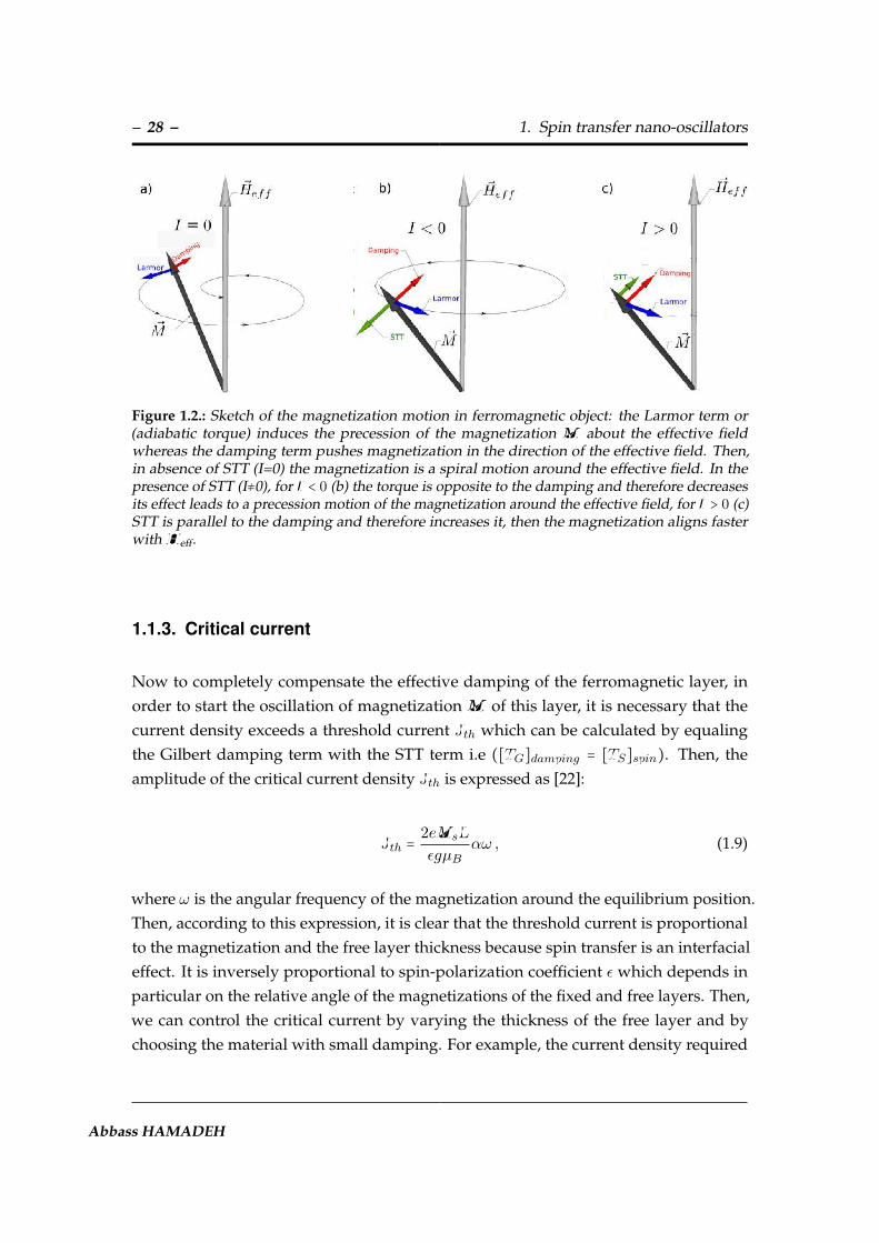
– 28 – 1. Spin transfer nano-oscillators
Figure 1.2.: Sketch of the magnetization motion in ferromagnetic object: the Larmor term or(adiabatic torque) induces the precession of the magnetization M about the effective fieldwhereas the damping term pushes magnetization in the direction of the effective field. Then,in absence of STT (I=0) the magnetization is a spiral motion around the effective field. In thepresence of STT (I≠0), for I < 0 (b) the torque is opposite to the damping and therefore decreasesits effect leads to a precession motion of the magnetization around the effective field, for I > 0 (c)STT is parallel to the damping and therefore increases it, then the magnetization aligns fasterwithHeff.
1.1.3. Critical current
Now to completely compensate the effective damping of the ferromagnetic layer, inorder to start the oscillation of magnetization M of this layer, it is necessary that thecurrent density exceeds a threshold current Jth which can be calculated by equalingthe Gilbert damping term with the STT term i.e ([TG]damping = [TS]spin). Then, theamplitude of the critical current density Jth is expressed as [22]:
Jth =2eMsL
εgµBαω , (1.9)
where ω is the angular frequency of the magnetization around the equilibrium position.Then, according to this expression, it is clear that the threshold current is proportionalto the magnetization and the free layer thickness because spin transfer is an interfacialeffect. It is inversely proportional to spin-polarization coefficient ε which depends inparticular on the relative angle of the magnetizations of the fixed and free layers. Then,we can control the critical current by varying the thickness of the free layer and bychoosing the material with small damping. For example, the current density required
Abbass HAMADEH

1.2. The vortex state – 29 –
for spin transfer effect for Permalloy of a few nm of thickness (α = 0.01, ω = 10 GHz, andε ∼ 0.5) is ∼ 107A/cm2.
1.2. The vortex state
The magnetic configuration at remanence inside a nanodot usually corresponds to aspatially non-uniform ground state. In certain conditions the magnetic configurationcould be in a vortex state. Indeed, the vortex state is often found to be the ground stateof magnetic nanodots, in which the dot size is larger than the exchange length LE ofthe material [65]. In the vortex state, the in-plane magnetizationM curls along the diskborder and in the center (the vortex core) the magnetization turns out-of-plane (seefigure 1.3). In fact, due to the finite size of a ferromagnetic disk the magnetization adoptsa vortex configuration at remanence to minimize the exchange and dipolar energies.In general, vortex nucleation can be favored in a ferromagnetic layer whose thicknessexceeds the exchange length LE and provided that the aspect ratio (thickness/lateralsize) is kept small, otherwise magnetic domain walls appear. The magnetic vortex ischaracterized by its chirality and polarity.
• The chirality C: this quantity defines the in plane direction of the magnetizationcurling and is either clockwise or counterclockwise ( C = ± 1).
• The polarity p: It defines the relative orientation of the vortex core with respect tothe plane of the ferromagnet. This quantity can be p = ± 1.
1.2.1. Static properties
To describe the vortex magnetization distribution, an analytical model has been proposedby Usov [66] which describes a rigid vortex core at the center of the disk. Indeed, fora circular dot of thickness L and radius R, the static magnetization distribution of thevortex can be parameterized as follows:
mx + imy = sin Θ(ρ)eiΦ(ρ), mz = p cos Θ(ρ), Φ(φ, ρ) = q φ +C π
2. (1.10)
Synchronization of spin trasnsfer nano-oscillators

– 30 – 1. Spin transfer nano-oscillators
Figure 1.3.: Figure (a) shows a sketch of a magnetic vortex of counterclockwise chirality andpositive polarity. Here the magnetization is curling in the plane of the disk, except at thecenter where it is pointing out-of-plane, This is called the vortex core. (b) and (c) shows thecharacteristics of a ferromagnetic vortex: polarity (b) and chirality (c).
Here ρ, φ, Θ and Φ are the polar coordinates that define the magnetization vector. Then,the common ansatz for the magnetization distribution in the core is [66]:
sin Θ(ρ) = 2ρRcR2c + ρ2
if ρ < Rc and Θ(ρ) = π2
if ρ > Rc . (1.11)
Where Rc corresponds to the vortex core radius which is a few exchange length (∼ 10- 20nm). In order to describe properly the evolution of magnetization distribution of themagnetic vortex and its dynamic properties, it is necessary to introduce an analyticaldescription of the vortex shifted from its equilibrium position. Several different analyticmodels of magnetic vortices in confined geometries were developed (see references[67, 65]). Thus, the magnetization of equation (1.10) is rewritten as:
mx + imy =2w(ζ, ζ)
1 +w(ζ, ζ)w(ζ, ζ), mz =
1 −w(ζ, ζ)w(ζ, ζ)1 +w(ζ, ζ)w(ζ, ζ)
, m2 = 1 , (1.12)
where ζ is a dimensionless variable and w(ζ, ζ) is a function which gives the position ofthe vortex core and it has the form:
Abbass HAMADEH
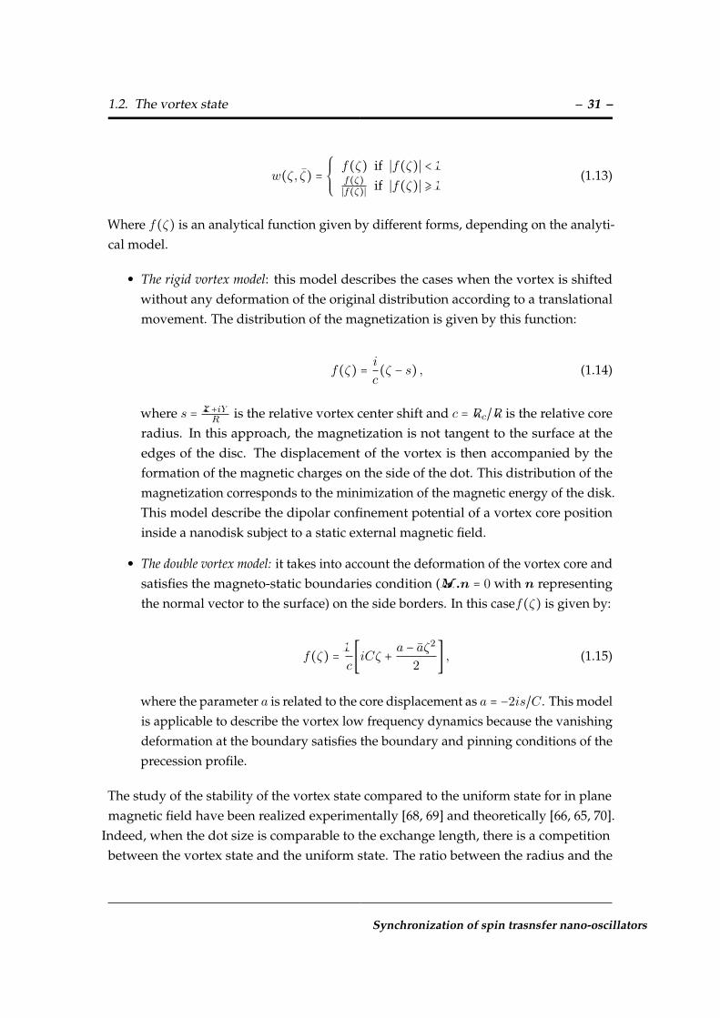
1.2. The vortex state – 31 –
w(ζ, ζ) =⎧⎪⎪⎨⎪⎪⎩
f(ζ) if ∣f(ζ)∣ < 1f(ζ)∣f(ζ)∣ if ∣f(ζ)∣ ⩾ 1
(1.13)
Where f(ζ) is an analytical function given by different forms, depending on the analyti-cal model.
• The rigid vortex model: this model describes the cases when the vortex is shiftedwithout any deformation of the original distribution according to a translationalmovement. The distribution of the magnetization is given by this function:
f(ζ) = ic(ζ − s) , (1.14)
where s = X+iYR is the relative vortex center shift and c = Rc/R is the relative core
radius. In this approach, the magnetization is not tangent to the surface at theedges of the disc. The displacement of the vortex is then accompanied by theformation of the magnetic charges on the side of the dot. This distribution of themagnetization corresponds to the minimization of the magnetic energy of the disk.This model describe the dipolar confinement potential of a vortex core positioninside a nanodisk subject to a static external magnetic field.
• The double vortex model: it takes into account the deformation of the vortex core andsatisfies the magneto-static boundaries condition (M.n = 0 with n representingthe normal vector to the surface) on the side borders. In this casef(ζ) is given by:
f(ζ) = 1
c[iCζ + a − aζ
2
2] , (1.15)
where the parameter a is related to the core displacement as a = −2is/C. This modelis applicable to describe the vortex low frequency dynamics because the vanishingdeformation at the boundary satisfies the boundary and pinning conditions of theprecession profile.
The study of the stability of the vortex state compared to the uniform state for in planemagnetic field have been realized experimentally [68, 69] and theoretically [66, 65, 70].
Indeed, when the dot size is comparable to the exchange length, there is a competitionbetween the vortex state and the uniform state. The ratio between the radius and the
Synchronization of spin trasnsfer nano-oscillators

– 32 – 1. Spin transfer nano-oscillators
Figure 1.4.: Diagram of stability of the vortex state (from[34]) when varying the dot radius R andthickness L (LE is the material exchange length). Three different ground state can be fonded. (I)vortex state, (II) magnetized uniformly in-plane and (III) magnetized uniformly parallel to thecylinder axis. The red area is a region of bi-stability.
thickness of the dot is the main parameter that is responsible to the transition betweenthese states. The boundaries between these states correspond to lines of equal magneticenergy. Then, the stability of a magnetic vortex in a soft ferromagnetic material wascalculated by Metlov et al. [65]. The calculation of energy for each dot aspect ratio L/Ris shown in figure 1.4. These calculations show that there are three stable magneticstates: the vortex state and the uniform states with the magnetization either in or out ofthe dot’s plane. Qualitatively, the phase diagram shows that if L or R is too small, themagnetization is saturated in the plane in the case of flat disk and the magnetization issaturated along the dot axis in the case of thick cylinder . Otherwise the vortex state isstable in soft magnetic cylinder with lateral size greater than the exchange length exceptin the bi-stability regions which corresponds to the red area in the figure 1.4.
Finally it should be mentioned that the phase diagram presented in figure 1.4 is universalfor soft magnetic dots if the geometrical sizes (R, L) are normalized to the materialexchange length LE .
1.2.1.1. Vortex stability under applied magnetic field
The stability of the vortex state as a function of magnetic field was studied in detailsin these references [71, 72, 67, 61]. The main effect of the external magnetic field is todeform the vortex configuration, and leading to its annihilation.
Abbass HAMADEH

1.2. The vortex state – 33 –
Figure 1.5.: Diagram of the reversal process of the normalized magnetization M/Ms as functionof in plane applied magnetic field of a magnetic disk. The remanent state corresponds to acentered vortex. The filled area represents the region of bi-stability between the vortex and theuniform state.
• In plane magnetic field: The stability of the vortex state as a function of in planemagnetic field was experimentally investigated for the first time by using magneto-optical measurements [69]. Indeed, when a strong magnetic field is applied inthe dot’s plane, the magnetization aligns with the field direction and thus thevortex is expulsed. In a magnetic disk with vortex state at zero field, the saturationmagnetization in the direction of the field is described by a process of vortex coredisplacement, and the vortex annihilation. The displacement of the vortex coreoccurs perpendicularly to the direction of the applied field due to the growth ofthe in-plane domain parallel to the applied field. The displacement of the corewas calculated by minimizing the total magnetic energy which consists of themagneto-static energy exchange and the Zeeman energy due to the external field.Figure 1.5 shows a typical behavior of the evolution of the magnetic vortex in adisk. When the magnetic field is decreased from the saturation, a magnetic vortexis nucleated, accompanied by an abrupt decrease in magnetization. The reversiblelinear part of the loop corresponds to the vortex core movement perpendicularto the applied field. Then, when the magnetic field reaches the annihilation field,the vortex vanishes completely and the disk stabilizes in a uniform state. Thefield annihilation (Han) of the vortex is greater than the field nucleation (Hn) ofthe vortex. There is also a region where the magnetic fields of the disk are in thebi-stable state (red area of figure 1.5). The values of characteristic fields (Han and
Synchronization of spin trasnsfer nano-oscillators
– 34 – 1. Spin transfer nano-oscillators
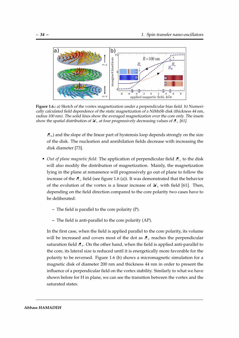
Figure 1.6.: a) Sketch of the vortex magnetization under a perpendicular bias field. b) Numeri-cally calculated field dependence of the static magnetization of a NiMnSb disk (thickness 44 nm,radius 100 nm). The solid lines show the averaged magnetization over the core only. The insetsshow the spatial distribution of Mz at four progressively decreasing values of H⊥ [61].
Hn) and the slope of the linear part of hysteresis loop depends strongly on the sizeof the disk. The nucleation and annihilation fields decrease with increasing thedisk diameter [73].
• Out of plane magnetic field: The application of perpendicular field H⊥ to the diskwill also modify the distribution of magnetization. Mainly, the magnetizationlying in the plane at remanence will progressively go out of plane to follow theincrease of the H⊥ field (see figure 1.6 (a)). It was demonstrated that the behaviorof the evolution of the vortex is a linear increase of Mz with field [61]. Then,depending on the field direction compared to the core polarity two cases have tobe deliberated:
– The field is parallel to the core polarity (P).
– The field is anti-parallel to the core polarity (AP).
In the first case, when the field is applied parallel to the core polarity, its volumewill be increased and covers most of the dot as Hz reaches the perpendicularsaturation field Hs. On the other hand, when the field is applied anti-parallel tothe core, its lateral size is reduced until it is energetically more favorable for thepolarity to be reversed. Figure 1.6 (b) shows a micromagnetic simulation for amagnetic disk of diameter 200 nm and thickness 44 nm in order to present theinfluence of a perpendicular field on the vortex stability. Similarly to what we haveshown before for H in plane, we can see the transition between the vortex and thesaturated states.
Abbass HAMADEH

1.2. The vortex state – 35 –
Figure 1.7.: Stability diagram of current (I) versus thickness L for Py discs with radius 100 nm.From [74]. The three states are stable in the shaded region.
1.2.1.2. Vortex stability under applied DC current
The influence of the DC current on the stability of the vortex was investigated in thisreference [74]. The main effect of a DC current on a ferromagnetic layer in the vortexstate is due to the Oersted field created by the current which is oriented in an ortho-radialdirection and its amplitude increases linearly from the center of the disk to its extremity.The Oersted field has a circular symmetry which is identical to the symmetry of thedistribution of the magnetization in the vortex state. Thus, for an Oersted field havingthe same chirality (direction of rotation) of the vortex, the magnetic state is favored, andvice versa in case of the opposite chirality (when the sign of the current is reversed).The stability of the vortex state, taking into account the effects of the Oersted field wascalculated by S. Urazhdin et al. [74]. Figure 1.7 shows the stability diagram calculationfor a permalloy disk (Ms = 800 emu/cm3) with a radius of 100 nm, varied thicknessL, and current I . Three different states can be distinguished. The state with positivechirality (C=+1), negative chirality (C=-1) and uniform state or single domain state. Inthis diagram the polarity I >0 is taken for the Oersted field of the current favoring theC=+1 state. The main conclusion of the phase diagram is as follows: although the initialconfiguration of a magnetic thin film (L<8nm) is uniform, it is possible to nucleate avortex by increasing the current amplitude. Then, if the thickness is sufficient, the vortexwill be stable even at zero current.
Synchronization of spin trasnsfer nano-oscillators

– 36 – 1. Spin transfer nano-oscillators
1.2.2. Gyrotropic mode
Several types of dynamic modes of magnetic vortices have to be distinguished, Thesemodes can be classified to two main types:
• The gyrotropic mode or translational mode which is excited at low frequency.
• The higher order modes (radial and azimuthal modes) which are excited at highfrequency (see section 2.3.2 of chapter 2).
The experiments performed in the vortex state in this thesis deal exclusively with thegyrotropic mode. In the following, we will provide some background on this mode.
The lowest energy excitation mode of a magnetic vortex is the so-called gyrotropic mode.It corresponds to a gyration of the vortex core around its equilibrium position at thecenter of the disk (see figure 1.8). In order to describe theoretically this mode, it is possibleto use an analytical model developed by Thiele [75]. Starting from the LLG equation, itcan be linearized and rewritten with the ansatz (M(ρ, t) =M(ρ −X(t), X(t)) and inthe presence of spin transfer torque, the full equation of motion is given :
G × X − ∂W (X)∂X
−DX +FSTT = 0 . (1.16)
WhereX parameterizes the vortex core position within the dot. In this equation the firstterm is a force acting perpendicular to the velocity. The gyrovector can be expressed asG = −G.ez , where G = 2πpLMs/γ, this vector is directed perpendicular to the disc plane,and is responsible for the vortex core oscillation. The second term is the reversible forceon the magnetic structure. This force is equal to a potential energy (W) that confines thecore in the middle of the disk. The variation of the total potential energy associated witha small displacement of the vortex core from the center can be expressed as :
W (X) =W (0) + κX2
2+O(X4) , (1.17)
the variation of the energy (W) is mainly due to the variation of the magnetostatic energy(Wms) and influence of the Oersted field induced by the current (WOe) [76].
Abbass HAMADEH

1.2. The vortex state – 37 –
Figure 1.8.: Scheme of the different forces acting on a vortex core which is represented by the reddot.
The third term is a dissipative force opposed to the velocity, responsible for the returnto equilibrium of the shifted vortex core. It can be shown that the tensor damping D isdiagonal [77] and that:
D ≃ −απMsL
γ[5
4+ ln
R
Rc] . (1.18)
The last term is the force due to the spin current which acts so as to compensate thedamping leading to steady precession of the core upon application of a dc current bias.In the case of a uniformly perpendicular polarized 2 current this torque has the form:
FSTT = κ⊥pzJ(Ð→ez ×Ð→X) , κ⊥ =
εMs
γπL . (1.19)
The different forces contributing to the gyrotropic motion of the vortex core are presentedin the figure 1.8. Here the vortex core is represented by red dot, which gyrates aroundan equilibrium orbit (red), defined by the balance between all the forces.
2These calculations of the terms of the equation have been done for the case of a uniformly polarizedcurrent [78, 76, 79]. For the other type of the polarizer orientation example vortex polarizer wherecertain simplifying assumptions can be made we can find the calculations in this reference [80].
Synchronization of spin trasnsfer nano-oscillators
– 38 – 1. Spin transfer nano-oscillators
Approximations for the gyrotropic-frequency
The calculation of eigen-frequency of the vortex oscillations can be done by solvingthe Thiele equation. The first calculation is given by Konstantin Guslienko, only thegyro-force and the confining potential are taken into account. Then, it predicts anoscillation frequency in the absence of applied magnetic field and zero current takes theapproximate form [81] :
ωG(0) ≃20
9γMs
L
R, (1.20)
which is a good approximation for disk with small thickness compared to the radius.Taking into account the presence of the applied current (the frequency of the oscillationsis modified due to the Oersted field created by the current [76, 82, 83]) and externalperpendicular magnetic field H⊥(See next chapter) [61], the frequency of the oscillationsis modified with respect to ωG(0) by two current and field dependent terms, so it takesthe form:
ω(H⊥) = ω0(H⊥) + ωOe(H⊥) with
⎧⎪⎪⎪⎪⎨⎪⎪⎪⎪⎩
ω0(H⊥) = ω0(0)[1 + pH⊥Hs].
ωOe(H⊥) = ωOe(0)√
1+[H⊥Hs
]
1−[H⊥Hs
]
.(1.21)
Where ωOe(0) ≃ 0.852π γµ0R.
Abbass HAMADEH

1.3. State-of-the-art of STNOs experimental results – 39 –
1.3. State-of-the-art of STNOs experimental results
Figure 1.9.: Upper panel: principle of spin transfer effect. Bottom panel : Two types of typicalspintronic devices (a) Nanopillar or (b) Nanocontact. In these typical devices two types ofmagnetic configurations can exist: homogeneous or vortex.
As mentioned in the introduction, the STNO microwave spintronic devices are basedon a magneto-resistive heterostructure of the type FMA/NM/FMB. Spin momentumtransfer from a current polarized by the polarizer FMA, to the local magnetizationof the free layer FMB can drive the latter into large angle self-sustained oscillations(see figure 1.9). This occurs when the spin polarized current is larger than a giventhreshold value, necessary to overcome intrinsic losses (see equation 1.9). These self-sustained oscillations are converted into voltage oscillations through magneto-resistive(MR) effects and are at the base of the spin transfer nano-oscillator (STNO) used formicrowave high frequency generation. After the first demonstration in 2003 by theCornell group [11] , many studies were realized in the following years to understand themagnetic excitations for different magnetic stack configurations, with varying magneticand transport properties, confirming the new phenomenon of spin momentum transferand its role for the magnetization dynamics. Several classes of configurations are usedthat are characterized by different excitation modes and frequency ranges. We give herea few examples of theses configuration in multi-layered nano-structures.
Synchronization of spin trasnsfer nano-oscillators
– 40 – 1. Spin transfer nano-oscillators
1.3.1. Individual STNOs
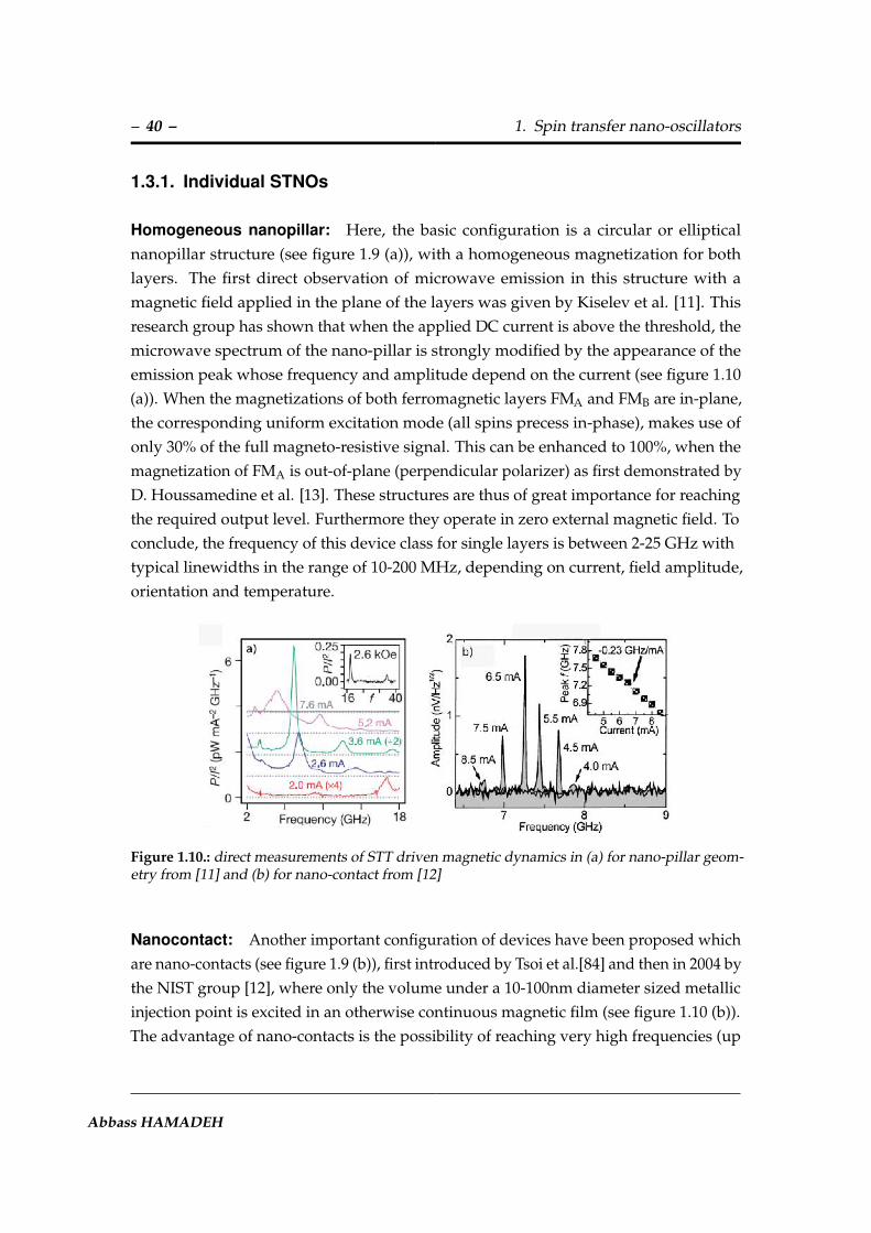
Homogeneous nanopillar: Here, the basic configuration is a circular or ellipticalnanopillar structure (see figure 1.9 (a)), with a homogeneous magnetization for bothlayers. The first direct observation of microwave emission in this structure with amagnetic field applied in the plane of the layers was given by Kiselev et al. [11]. Thisresearch group has shown that when the applied DC current is above the threshold, themicrowave spectrum of the nano-pillar is strongly modified by the appearance of theemission peak whose frequency and amplitude depend on the current (see figure 1.10(a)). When the magnetizations of both ferromagnetic layers FMA and FMB are in-plane,the corresponding uniform excitation mode (all spins precess in-phase), makes use ofonly 30% of the full magneto-resistive signal. This can be enhanced to 100%, when themagnetization of FMA is out-of-plane (perpendicular polarizer) as first demonstrated byD. Houssamedine et al. [13]. These structures are thus of great importance for reachingthe required output level. Furthermore they operate in zero external magnetic field. Toconclude, the frequency of this device class for single layers is between 2-25 GHz withtypical linewidths in the range of 10-200 MHz, depending on current, field amplitude,orientation and temperature.
Figure 1.10.: direct measurements of STT driven magnetic dynamics in (a) for nano-pillar geom-etry from [11] and (b) for nano-contact from [12]
Nanocontact: Another important configuration of devices have been proposed whichare nano-contacts (see figure 1.9 (b)), first introduced by Tsoi et al.[84] and then in 2004 bythe NIST group [12], where only the volume under a 10-100nm diameter sized metallicinjection point is excited in an otherwise continuous magnetic film (see figure 1.10 (b)).The advantage of nano-contacts is the possibility of reaching very high frequencies (up
Abbass HAMADEH

1.3. State-of-the-art of STNOs experimental results – 41 –
to 65 GHz) as has been demonstrated by Bonetti et al .[14] and to easily realize couplingof individual oscillators via spin waves (see next section).
Vortex based STNOs: The ability to induce steady oscillations in a ferromagnet byusing a DC current, has firstly been reported only for a uniform magnetization. Subse-quently, a second case of dynamics that was foretold to be possible as a result of STT aresteady oscillations of non-uniform magnetic structure (magnetic vortex) under excitationby a direct DC current. Several experiments have indeed demonstrated this phenomenonin different geometries. The initial experiments was given by the group from Cornelluniversity [33] in a nanopillar device. In this geometry, the microwave signals wereobserved for out-of-plane applied fields (required to have a polarized layer which ishere essential for the vortex to be excited into steady motion). Here the spin transfertorque acts as a source of anti-damping, canceling out the damping torque on averagean thus leading to the oscillation of the vortex. Then, thanks to the magneto-resistance,the oscillations of the voltage at frequencies below 2 GHz are observed, correspondingto oscillations of the gyrotropic mode (see figure 1.11). This vortex mode, first intro-duced in nano-pillar geometry followed in 2008 by [79] in nano-contact geometry. Theseoutcomes, quickly aroused great interest of the scientific community because the vortexmode offers important advantages compared the homogenous modes, to mention are alower threshold current a lower linewidth (<1MHz) , easier stabilization of modes inzero field [85] and up to 100% use of the magnetoresistance (thus large output power)due to the large radius of the trajectory [76, 35].
Figure 1.11.: Experimental measurement of the microwave signal resulting from the motion ofthe gyro-tropic vortex core under the influence of the spin transfer torque. Sample layout (leftinset). Microwave peak which can be obtained at ∼ 6 Oe (right inset). From [33].
Synchronization of spin trasnsfer nano-oscillators

– 42 – 1. Spin transfer nano-oscillators
Single STNOs with improved performance
The integration of STNOs in high frequency circuits depends on various conditions. Theimportant parameters are linewidth, and the generated power signal. Further researchefforts are being devoted to optimization of these parameters. In the last 6 years, thestate of the art for STNO power performances has increased by more than 40dB, mainlythrough the use of magnetic tunnel junctions (MTJ). To date, the largest power outputobtained in a single MTJ device in the vortex state is close to the µW range for a TMRhybrid device [35, 36, 86].
A remaining key issue is the phase noise directly related to linewidth. Using specialnanocontact geometry, subsequent reports showed a reduction from GHz down to a fewMHz by using a strong out-of-plane field [87]. A recent research allowed identifyingtwo main origins of the spectral linewidth. First, as the active magnetic volume in suchspin transfer devices is extremely small (<< µm3), the magnetic energy at stake is ofthe order of the thermal energy, meaning that thermal noise determines for the mostpart the generation linewidth [88, 23]. Second, the high nonlinear character of STNOs(i.e. the dependence of the frequency on the precession amplitude and with this on thespin polarized current) is extremely important for achieving high frequency tunabilityunreachable for any other types of oscillators, but in turn, is a source of phase noise[89, 90, 25].
Although the understanding of the linewidth broadening is still a subject of intenseresearch, it was recently identified an important way for linewidth reduction, whichmakes use of collective excitations. Going beyond excitations in a single magnetic layeras done in the large majority of studies, the use of magnetic multilayer stacks is aninnovative point proposed in several studies. In such structures like FM/NM/FM, alllayers interact directly via spin transfer torque as well as dipolar interactions. Recently,Houssameddine et al . have shown that the linewidth in an anti-ferromagnetic exchangecoupled bilayer is by a factor of 10 narrower than the one of a single layer [38]. ThenCNRS/Thales in collaboration with CEA/SPEC have shown that in spin transfer oscilla-tors based on coupled vortices, the linewidth drops down to a minimum of 50 kHz [40]as compared to 1 MHz in a single layer.
Finally, Naletov et al. [41] have succeeded to identify selection rules for the excited modesfor a single nano-pillar that are of importance when coupling the oscillations of differentlayers or when synchronizing to an external signal source. This fundamental aspect
Abbass HAMADEH
1.3. State-of-the-art of STNOs experimental results – 43 –
is vital for improving the spectral purity via synchronization of different oscillators orinside a phase locked loop.
1.3.2. Phase-locking and mutual synchronization
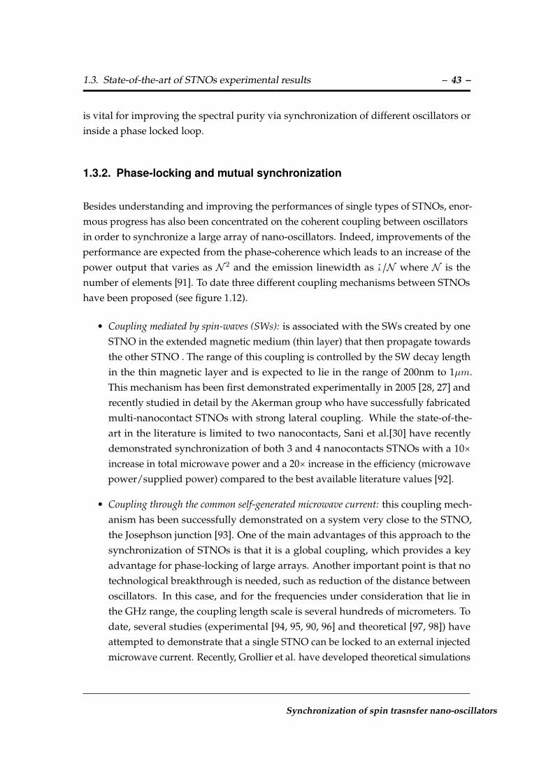
Besides understanding and improving the performances of single types of STNOs, enor-mous progress has also been concentrated on the coherent coupling between oscillatorsin order to synchronize a large array of nano-oscillators. Indeed, improvements of theperformance are expected from the phase-coherence which leads to an increase of thepower output that varies as N 2 and the emission linewidth as 1/N where N is thenumber of elements [91]. To date three different coupling mechanisms between STNOshave been proposed (see figure 1.12).
• Coupling mediated by spin-waves (SWs): is associated with the SWs created by oneSTNO in the extended magnetic medium (thin layer) that then propagate towardsthe other STNO . The range of this coupling is controlled by the SW decay lengthin the thin magnetic layer and is expected to lie in the range of 200nm to 1µm.This mechanism has been first demonstrated experimentally in 2005 [28, 27] andrecently studied in detail by the Akerman group who have successfully fabricatedmulti-nanocontact STNOs with strong lateral coupling. While the state-of-the-art in the literature is limited to two nanocontacts, Sani et al.[30] have recentlydemonstrated synchronization of both 3 and 4 nanocontacts STNOs with a 10×increase in total microwave power and a 20× increase in the efficiency (microwavepower/supplied power) compared to the best available literature values [92].
• Coupling through the common self-generated microwave current: this coupling mech-anism has been successfully demonstrated on a system very close to the STNO,the Josephson junction [93]. One of the main advantages of this approach to thesynchronization of STNOs is that it is a global coupling, which provides a keyadvantage for phase-locking of large arrays. Another important point is that notechnological breakthrough is needed, such as reduction of the distance betweenoscillators. In this case, and for the frequencies under consideration that lie inthe GHz range, the coupling length scale is several hundreds of micrometers. Todate, several studies (experimental [94, 95, 90, 96] and theoretical [97, 98]) haveattempted to demonstrate that a single STNO can be locked to an external injectedmicrowave current. Recently, Grollier et al. have developed theoretical simulations
Synchronization of spin trasnsfer nano-oscillators

– 44 – 1. Spin transfer nano-oscillators
[26], within the macro-spin approximation, which show that synchronization ofan assembly of STNOs is achievable through the common stimulated microwavecurrent. These calculations, performed at zero temperature, provide evidence thatthe efficiency of phase-locking is strongly linked to the MR ratio of each oscillatorand to the delay of microwave current transmission between STNOs. To date thereis no experimental verification of this coupling mechanism, because of the toosmall rf emitted power and the too large phase noise of individual STNOs.
• Coupling through the dipolar magnetic field: when the separation between STNOsis reduced to approximately their diameter, the oscillations in the individualoscillators can couple via the dynamic magnetic dipolar fields radiated from eachSTNO. Several experimental studies have demonstrated that a single STNO can belocked to the rf magnetic field produced by an external microwave antenna [99].Then, in the resonance mode (below threshold excitation) this coupling has recentlybeen demonstrated by Pigeau et al. using the MRFM technique [100]. It mightproof to be more efficient than electrical coupling and spin-waves coupling, thisis why we decided to perform a first experimental study using only two STNOsplaced nearby laterally. The experimental result of this study will be presented inchapter 8.
Abbass HAMADEH

1.3. State-of-the-art of STNOs experimental results – 45 –
Figure 1.12.: Summary of state of art of phase locking and mutual synchronization.
Synchronization of spin trasnsfer nano-oscillators
– 46 – 1. Spin transfer nano-oscillators
In conclusion, we have presented in this chapter the basic operating concepts ofSTNOs. They offer many capabilities for applications, but many challenges remainin order to optimize the microwave performances of these spintronic devices. In par-ticular, vortex based STNOs, STNOs operating on coupled modes, and the couplingof several STNOs are promising ways to achieve this goal.
Abbass HAMADEH

CHAPTER 2
Classification of spin-wave modes in magnetic nanostructures
In this chapter, we first introduce the basics of a general theoretical approach of linearspin-wave excitations. We then present the classification of spin-wave modes in twoparticular cases of interest in this thesis, which both preserve the axial symmetry: thenormally saturated disk, and the vortex-state disk, in the presence of a perpendicularmagnetic field. We then discuss the influence of dipolar interaction on the collectivedynamics of adjacent magnetic disks.
47
– 48 – 2. Classification of spin-wave modes in magnetic nanostructures
2.1. General approach
The general theoretical framework to determine linear spin wave modes in magneticnanostructures, developed by Vasyl Tiberkevich and Andrei Slavin, is presented indetails in references [41, 101] and in the thesis of Benjamin Pigeau [102]. Below, webriefly recall the general idea of this approach.
The first step is the linearization of the Landau-Lifshitz equation of motion of magneti-zation
∂M
∂t= γHeff ×M , (2.1)
in which the non-conservative terms are disregarded, and where the effective field,introduced in equation (2), can be conveniently written in the following form:
Heff =Hext − 4πG ∗M . (2.2)
In this notation, G is a linear tensor self-adjoint operator that regroups all the internalmagnetic interactions (exchange, demagnetizing and magneto-crystalline anisotropyenergies).
In the equilibrium state, the effective field Heff is parallel everywhere to the localmagnetization direction uM . To find the linear magnetization excitations, the out-of-equilibrium component of the magnetizationm is defined by the following ansatz:
M(r, t) =Ms(uM +m(r, t)) +O(m2) . (2.3)
The norm of the magnetization vector is a constant of motion, hencem.uM = 0. Thus,mis the small component of the magnetization (∣m∣ ≪ 1) oscillating in the plane transverseto the local uM .
Substitutingm in equation (2.1) and keeping only the linear terms, a linear equation de-scribing the transverse magnetization precession at the Larmor frequency is obtained:
∂m
∂t= uM × Ω ∗m , (2.4)
where the sign ∗ denotes the convolution product. The self-adjoint tensor operator Ω
represents here the Larmor frequency:
Ω = γ(HeffI + 4πMsG) . (2.5)
Abbass HAMADEH

2.1. General approach – 49 –
Here, I is the identity matrix and Heff is the norm of the effective field.
Considering only linear excitations of the spin system,m is developed in the eigen-basisof the spin wave eigenmodes, labeled by ν:
m(r, t) ≈∑ν
cν(t)mν(r) + c.c. (2.6)
where c.c. stands for complex conjugate. In this formulation, cν(t) are the amplitudesof the eigenmodes and mν(r) represents their spatial profile. This eigen-basis must beorthonormal and obey the closure relation:
i⟨mν .(uM ×mν′ )⟩ = Nνδν,ν , (2.7)
where m is the c.c. of m, δ the Kronecker delta function, and the bracket denotes thespatial average over the volume of the magnetic body. Nν are normalization constantsof the basis.
Assuming an oscillatory dependence of the spin wave magnetization vector mν at theeigen-frequencies ων , the eigen-modes labeled by ν are solutions of equation (2.4):
− iωνmν = uM × Ω ∗mν . (2.8)
The main properties of spin wave excitations follow from the eigen-problem equation(2.8) and the fact that the operator Ω is self-adjoint and real. In particular, if the equi-librium magnetization along uM corresponds to a local minimum of the energy, theoperator Ω is positive-definite. The “physical” (positive) eigen-frequencies are thensimply given by the formula:
ων =⟨mν .Ω ∗mν⟩
Nν. (2.9)
The importance of this relation is that the frequenciesων calculated using equation (2.9)are variationally stable with respect to perturbations of the mode profile mν . Thus,injecting some trial vectors inside equation (2.9) allows one to get approximate values ofων with high accuracy.
Synchronization of spin trasnsfer nano-oscillators
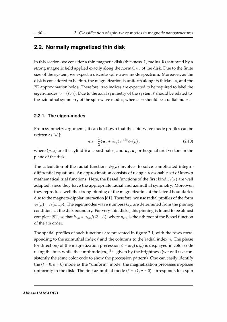
– 50 – 2. Classification of spin-wave modes in magnetic nanostructures
2.2. Normally magnetized thin disk
In this section, we consider a thin magnetic disk (thickness L, radius R) saturated by astrong magnetic field applied exactly along the normal uz of the disk. Due to the finitesize of the system, we expect a discrete spin-wave mode spectrum. Moreover, as thedisk is considered to be thin, the magnetization is uniform along its thickness, and the2D approximation holds. Therefore, two indices are expected to be required to label theeigen-modes: ν = (`, n). Due to the axial symmetry of the system,` should be related tothe azimuthal symmetry of the spin-wave modes, whereas n should be a radial index.
2.2.1. The eigen-modes
From symmetry arguments, it can be shown that the spin-wave mode profiles can bewritten as [41]:
m` =1
2(ux + iuy)e−i`φψ`(ρ) , (2.10)
where (ρ,φ) are the cylindrical coordinates, and ux, uy orthogonal unit vectors in theplane of the disk.
The calculation of the radial functions ψ`(ρ) involves to solve complicated integro-differential equations. An approximation consists of using a reasonable set of knownmathematical trial functions. Here, the Bessel functions of the first kind J`(x) are welladapted, since they have the appropriate radial and azimuthal symmetry. Moreover,they reproduce well the strong pinning of the magnetization at the lateral boundariesdue to the magneto-dipolar interaction [81]. Therefore, we use radial profiles of the formψ`(ρ) = J`(kl,nρ). The eigenmodes wave numberskl,n are determined from the pinningconditions at the disk boundary. For very thin disks, this pinning is found to be almostcomplete [81], so that k`,n = κ`,n/(R+L), where κ`,n is the nth root of the Bessel functionof the `th order.
The spatial profiles of such functions are presented in figure 2.1, with the rows corre-sponding to the azimuthal index ` and the columns to the radial index n. The phase(or direction) of the magnetization precession φ = arg(mν) is displayed in color codeusing the hue, while the amplitude ∣mν ∣2 is given by the brightness (we will use con-sistently the same color code to show the precession pattern). One can easily identifythe (` = 0, n = 0) mode as the “uniform” mode: the magnetization precesses in-phaseuniformly in the disk. The first azimuthal mode (` = +1, n = 0) corresponds to a spin
Abbass HAMADEH

2.2. Normally magnetized thin disk – 51 –
Figure 2.1.: Color representation of the Bessel spatial patterns for different values of the azimuthalmode index ` (by row) and radial mode index n (by column). The arrows are a snapshot ofthe transverse magnetization mν , labeled by the index ν = (`, n). All arrows are rotatingsynchronously in-plane at the spin-wave eigen-frequency. The hue indicates the phase φ =arg(mν) (or direction) of mν , and the brightness the amplitude of ∣mν ∣2. The nodal positions(∣mν ∣ = 0) are marked in white.
Synchronization of spin trasnsfer nano-oscillators

– 52 – 2. Classification of spin-wave modes in magnetic nanostructures
wave that is rotating around the disk in the same direction as the Larmor precession.The corresponding phase is in quadrature between two orthogonal positions and thismode has a node at the center of the disk (the nodal positions are marked in white).Then, increasing the index n results in an increase of the number of nodes in the radialdirection.
2.2.2. Selection rules
The spatial symmetry of the source is crucial to determine which spin-wave eigen-modescan be excited [41]. The overlap integral between the excitation field hrf and the modeprofile governs the selection rules:
h`,n =⟨m`,n.hrf ⟩N`,n
. (2.11)
It can be easily shown that a uniform microwave magnetic field can only excite (` = 0, n)spin wave modes, because in this case overlap integrals with azimuthal modes (` ≠ 0)vanish. In order to excite azimuthal spin wave modes with ` = +1, a field with anorthoradial symmetry can be used, as the one produced by an rf current flowing verticallythrough the disk [41]. We will come back on this point in section 5.5 of chapter 5
2.2.3. Influence of symmetry breaking
In the case of a small symmetry breaking from the perfect axial symmetry, introducedeither by a small tilt of the perpendicular applied field [59, 41] or a deviation from aperfect circular shape of the disk [41], it is still possible to use the same eigen-basis ofequation (2.10) to decompose the new spin-wave modes. The so-called “uniform” modewill not be affected, as it will always correspond to an in-phase precession of all thespins around the local effective field. But in general, the eigen-modes will now be asuperposition of ` = 0 and ` ≠ 0 modes of the basis, therefore, the selection rules mightalso be affected [59, 41].
Abbass HAMADEH

2.3. Disk in the vortex state – 53 –
Figure 2.2.: Profile of the vortex gyrotropic mode in the regime of small (a) and large (b) ampli-tude. The dashed circle displays the vortex core orbit, which is smaller and larger than the coreradius in (a) and (b), respectively.
2.3. Disk in the vortex state
We have already introduced in section 1.2 the particular dynamics of the gyrotropicmode in the vortex state with no applied magnetic field. Although the Thiele equationis very convenient to describe the dynamics of the vortex core, it is interesting to notethat this gyrotropic mode can be treated in the same general framework as presentedin section 2.1, see e.g. reference [103]. In particular, similarly to equation 2.3, the profileof the gyrotropic mode can be defined as the dynamical deviation from equilibriumconfiguration,m =M(x, y) −M(x, y)eq, where x, y are the cartesian coordinates in thedisk. Using the same color code as in figure 2.1, we have plotted in figure 2.2 (a) thisprofile in the linear regime, where the deviation of the vortex core from its equilibirumposition at the center of the disk is smaller than the core radius. From this snapshot ata particular phase of the vortex core gyration, it is clear that the gyrotropic mode hasthe ` = 0 symmetry, as the arrows displaying the dynamical magnetization are pointingon average in a particular direction (mainly along −Y). At larger radius of gyration(figure 2.2 (b)), we observe that the magnetization in the central region enclosed by thecore orbit (see dashed circle) operates a full rotation in the plane over one period. Thisfeature was also clear from the Thiele approach presentend in section 1.2.2 and is a veryinteresting point for the power emitted by STNOs based on the gyrotropic mode. It isalso interesting to note that the dynamical magnetization profile extend far outside theregion enclosed by the core orbit, until the boundaries of the disk.
Synchronization of spin trasnsfer nano-oscillators
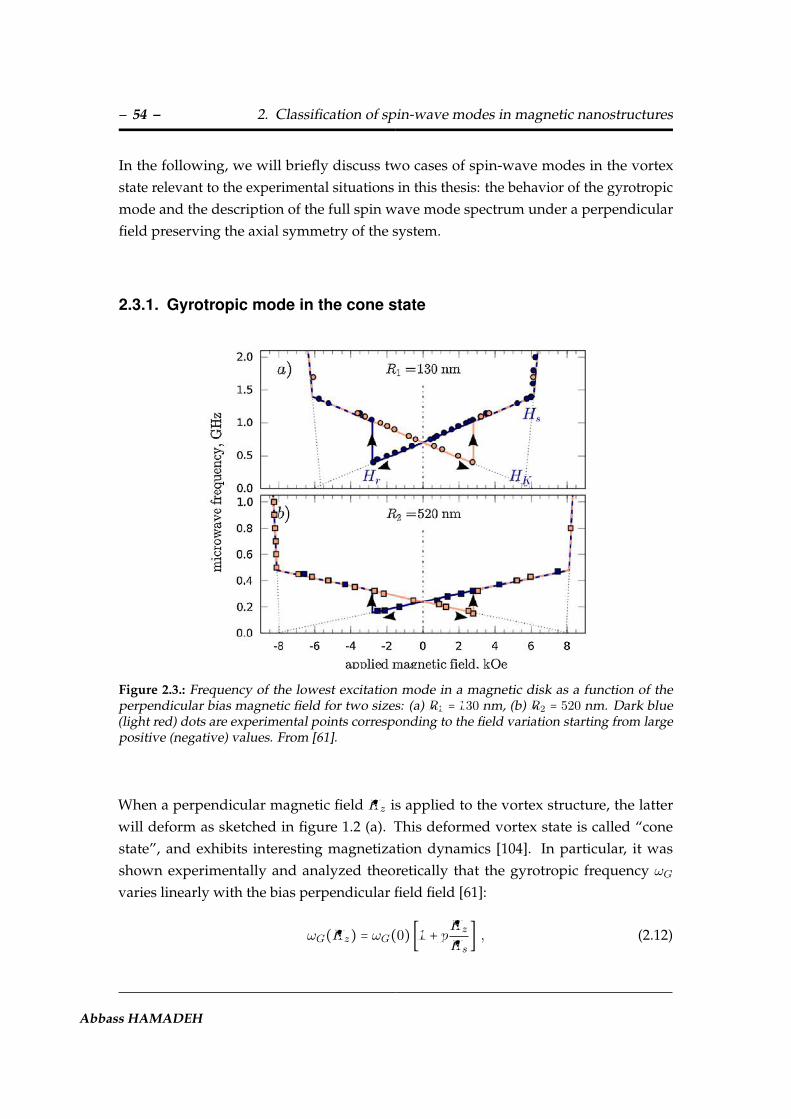
– 54 – 2. Classification of spin-wave modes in magnetic nanostructures
In the following, we will briefly discuss two cases of spin-wave modes in the vortexstate relevant to the experimental situations in this thesis: the behavior of the gyrotropicmode and the description of the full spin wave mode spectrum under a perpendicularfield preserving the axial symmetry of the system.
2.3.1. Gyrotropic mode in the cone state
Figure 2.3.: Frequency of the lowest excitation mode in a magnetic disk as a function of theperpendicular bias magnetic field for two sizes: (a) R1 = 130 nm, (b) R2 = 520 nm. Dark blue(light red) dots are experimental points corresponding to the field variation starting from largepositive (negative) values. From [61].
When a perpendicular magnetic field Hz is applied to the vortex structure, the latterwill deform as sketched in figure 1.2 (a). This deformed vortex state is called “conestate”, and exhibits interesting magnetization dynamics [104]. In particular, it wasshown experimentally and analyzed theoretically that the gyrotropic frequency ωG
varies linearly with the bias perpendicular field field [61]:
ωG(Hz) = ωG(0) [1 + pHz
Hs] , (2.12)
Abbass HAMADEH
2.3. Disk in the vortex state – 55 –
where Hs is the perpendicular saturation field of the disk. Two different frequencybranches can be observed, depending on the the vortex core polarity p, as shown infigure 2.3. When p is anti-parallel to Hz (p.Hz < 0) equation (2.12) is valid only if theperpendicular field is below the static reversal field Hr, which is indicated in figure 1.6(a) of chapter 1 and figure 2.3.
From equation (2.12), it is interesting to note that the vortex core polarity is directlygiven by the slope of ωG(Hz) vs. Hz . If ωG(Hz) increases (decreases) as Hz increases,then p = +1 (p = −1), i.e., the vortex core is along+z (−z). This useful property will allowus to determine the orientation of the vortex core in our experimental results presentedin chapters 7 and 8.
2.3.2. Higher order spin-wave modes
The gyrotropic mode is the lowest energy mode of the vortex state, and in this thesis, wewill operate STNOs based on this mode. However, there are of course many other spin-wave modes at higher energy [105, 106, 107, 108]. Here, we briefly mention the natureof these modes, and we comment on the large frequency gap which exists between thegyrotropic mode and higher order spin-wave modes in the vortex state.
The general approach presented in section 2.1 can be applied to classify the spin-wavemodes in the vortex state. The obtained spin wave spectrum is similar to the normallysaturated state, with the existence of radial and azimuthal modes. However, somequalitative differences exist due to the presence of the vortex core at the center of thedisk, and to the orthoradial symmetry of the equilibrium magnetization in the vortexstate (see figure 1.3 of chapter 1).
1. Radial spin waves (` = 0, n). Similarly to the case of a normally saturated disk, radialspin waves develop in the disk plane, leading to a varying angle of precession inthe radial direction [108]. In the limit of thin disks, the amplitude of the dynamicalmagnetization is well described by Bessel functions [105, 108]. The presence ofthe vortex core does not break the symmetry, but imposes a vanishing angle ofprecession at the center of the disk. Therefore, J1 rather than J0 is appropriateto describe the mode profiles, because J1(0) = 0. Compared to the saturatedstate, the symmetry of the background in which the spin wave modes developis inverted. Out of the core, the magnetization follows an orthoradial symmetry,while it was axial in the saturated case. Therefore, the selection rules for these spin
Synchronization of spin trasnsfer nano-oscillators

– 56 – 2. Classification of spin-wave modes in magnetic nanostructures
Figure 2.4.: In plane dynamical susceptibilities a)χ− and b) χ+ for a downward field sweep anda positive field branch (p = +1). The high values are in black and the low ones in light gray.
waves are reversed: to couple to the radial modes in the vortex state, the excitationhas to follow an azimuthal symmetry. For instance, a microwave field appliedperpendicularly to the plane of the disk is effective [108].
2. Azimuthal spin waves (`, n = 0). Waves traveling around the vortex core can alsobe excited. The profiles of these modes are proportional to m`(ρ) cos(`φ + ω`,0t).In a saturated disk, azimuthal spin waves with indices ±`, traveling in oppositedirections, are degenerate in energy. The presence of the vortex core lifts thisdegeneracy [109]. In fact, the gyrotropic mode can interact with the azimuthalmodes by dynamic dipolar coupling [103], leading to a lower (higher) frequencyfor waves rotating with (against) the gyrotropic mode. The selection rules forthese modes are also reversed compared to the saturated state, as they can only beexcited by a spatially homogeneous in-plane microwave field.
In figure 2.4, we present the results of micro-magnetic simulations which illustrate thequalitative modification of the spin-wave spectrum between the normally saturatedand the vortex (cone) states [110]. Here, the dynamic susceptibility tensor χi,j(r, ω)
Abbass HAMADEH

2.3. Disk in the vortex state – 57 –
(i, j = x, y, z) of a Permalloy disk (L = 50 nm, R = 500 nm) is calculated using a 3Dmicro-magnetic code [110]. Due to the rotational symmetry of the element, the in-planesusceptibility spectra are expressed using the circular polarization basis resulting inχ± = 1/2[(χxx + χyy) ± i(χyx − χxy)]. The imaginary part of both quantities are plottedversus the perpendicular field Hz in figure 2.4.
In the saturated state (Hz > Hs ≃ 9.5 kOe), the radial modes (` = 0, n) described in thesection 2.2 are seen in the χ− component. Azimuthal modes (`, n = 0) are not observedbecause they do not couple to the homogeneous in-plane microwave excitation field. Inthe vortex state (Hz <Hs), the low frequency gyrotropic mode is identified as 0−. It hasthe expected dependence versus field for a p = +1 core polarity and couples only to χ−because of the particular sense of rotation of the core. At higher frequency, several spinwave modes can be seen. They exhibit an opposite dependence with Hz . In contrastto the saturated state, they correspond to azimuthal modes. The magnetization of thevortex is curling in-plane, hence, the in-plane excitation field cannot couple to the radialmodes. The azimuthal modes can travel either clockwise or counter-clockwise aroundthe disk, this is the reason why they can be observed both in χ− and χ+. Moreover, themodes having indices l = ±1,2 are not degenerate in energy.
A particularly interesting observation is the existence of a large gap between the fun-damental gyrotropic mode and higher order spin-wave modes in the vortex state (inthis example, more than 5 GHz at zero field), in contrast to the saturated case (wherethis gap is lower than 0.5 GHz). This well isolated fundamental mode makes it anideal candidate to operate STNOs [33, 35], as the presence of neighboring spin-wavemodes in the spectrum is known to affect negatively the coherence of auto-oscillations[88, 111, 112].
Synchronization of spin trasnsfer nano-oscillators

– 58 – 2. Classification of spin-wave modes in magnetic nanostructures
2.4. Collective spin-wave modes induced by the dipolarinteraction in a pair of magnetic disks
In this section, we introduce the notion of coupled dynamics between neighboring disksinteracting through dipolar magnetic fields. Due to the different experimental cases metin this thesis, we will discuss the particularities due to the geometry (vertical vs. lateralarrangement of the disks) and to the ground state (normally saturated vs. vortex) in afirst step, by explaining how to evaluate the strength of the magneto-dipolar coupling.In a second step, we will treat the coupled equations of motion from a general point ofview in order to describe the basics of the resulting collective dynamics.
2.4.1. Strength of the dynamic magneto-dipolar coupling
The goal here is to evaluate the strength of the dynamic dipolar coupling betweenadjacent disks. The general expression of the effective demagnetizing stray field pro-duced by the dynamic magnetization of the jth disk projected along the local dynamicalmagnetization vector inside the ith disk and averaged over its volume is given by
hi→j =Ms
Nj⟨mj .Gd ∗mi⟩Vj , (2.13)
where Gd is the contribution of the demagnetizing interaction of the linear tensor self-adjoint operator introduced in equation (2.2).
The overlap defined in equation (2.13) is maximum for modes having the same wavenumbers in each disk [113]. In the following, we will thus only consider the dynamicdipolar coupling between similar spin-wave modes. Hence,mj and mi correspond tothe dynamical magnetization in each of the disks, but they have the same set of modeindices (`,m). Two cases are particularly interesting to us: the uniform mode in thenormally saturated state (with spatial profile J0(k0,0ρ)) and the gyrotropic mode in thevortex state (in this case, the spatial profile of the gyrotropic mode defined in reference[103] should be employed).
This dynamical field is an in-plane rotating field that is able to couple to the dynamicalpart of magnetization in both disks. Its calculation is in general non trivial, but can bederived in some simple cases [114, 41, 115, 116]. Generally, it can be calculated from
Abbass HAMADEH

2.4. Collective spin-wave modes induced by the dipolar interaction – 59 –
the demagnetizing tensor N . In the case of two discs on top of each other, this field isisotropic since N i→j
xx = N i→jyy , hence
hi→j =MsN i→jxx , (2.14)
where the curly brackets indicate that the spatial average is weighted by the mode profile.But in the case of two disks placed side by side, the axial symmetry is broken and:
hi→j =Ms
2(N i→j
xx + N i→jyy ) . (2.15)
Finally, we would like to point out the strong dependence of the dynamic magneto-dipolar coupling on the geometry. Roughly, it indeed scales with the thickness ofthe magnetic layers L and decays as 1/d3, where d is the spacing between magneticelements.
2.4.2. Coupled equations of motion and collective dynamics
Denoting the spin wave amplitudes in both disks by c1,2 and their isolated frequenciesby ω1,2, the coupled equations neglecting the damping terms read:
dc1
dt= −iω1c1 + iγh2→1c2 (2.16a)
dc2
dt= −iω2c2 + iγh1→2c1 (2.16b)
By diagonalizing this system, the eigenvalues of the coupled frequencies ωA,B are foundto be:
ωA,B = ω1 + ω2
2±
¿ÁÁÀ(ω1 − ω2
2)
2
+ (Ω
2)
2
, (2.17)
where the coupling strength is:
Ω2 = 4γ2h1→2h2→1 . (2.18)
The anti-crossing (or avoided crossing) behavior of equation (2.17), shown in figure 2.5(a), is typical of two oscillators coupled by conservative terms.
The collective eigen-modes are given by the eigen-vectors of the system, and are linear
Synchronization of spin trasnsfer nano-oscillators

– 60 – 2. Classification of spin-wave modes in magnetic nanostructures
combinations of the isolated spin-wave modes in each disk:
CA = c1 +ω1 − ωAγh2→1
c2 (2.19a)
CB = ω2 − ωBγh1→2
c1 + c2 . (2.19b)
The ratio of hybridization is given by
cicj
∣ωA,B
=⎛⎝(ωi − ωj) ∓
√(ωi − ωj)2 +Ω2
Ω
⎞⎠
∓1
. (2.20)
In the case of lateral neighboring disks displayed in figure 2.5 (b), the anti-binding modeA with higher energy has ci = −cj , i.e., a precession with equal weight in both disks andout-of-phase (optical mode), and the binding mode B with lower energy has ci = +cjwhich denotes an in-phase precession (acoustic mode). Due to the reversed sign of thedipolar interaction, the situation is opposite in the case of vertically stacked disks.
To conclude, the dynamic dipolar interaction between neighboring magnetic disks hastwo main consequences:
1. It renormalizes the eigen-frequencies following equation (2.17).
2. It hybridizes the spin-wave modes, which become delocalized in both magneticelements (see equation (2.20)).
To experimentally observe these effects, however, the dynamic dipolar coupling Ω hasto be large with respect to the mismatch ω2 − ω1 between the isolated (uncoupled)frequencies, but also with respect to the linewidth of the resonance line [100].
Abbass HAMADEH

2.4. Collective spin-wave modes induced by the dipolar interaction – 61 –
Figure 2.5.: (a) Eigen-frequencies vs. mismatch between isolated frequencies. (b) Energy leveldiagram when ω1 = ω2. The magneto-dipolar interaction hybridizes the system in binding andanti-binding coupled modes separated in frequency by the dynamical splitting Ω.
To summarize, we have presented a general analytical theory which enables to calcu-late the frequencies of the spin-wave eigen-modes in the linear regime and to clas-sify them according to their symmetry. In a normally magnetized disk, azimuthaland radial indices (`, n) are required to label the spin-wave modes. We have alsodescribed the influence of a perpendicular magnetic field on the spin-wave modesin the vortex-state. Finally, we have highlighted that the dynamic dipolar interactionbetween neighboring magnetic elements hybridizes the spin-wave modes, which be-come coupled, and renormalizes their eigen-frequencies.
Synchronization of spin trasnsfer nano-oscillators

CHAPTER 3
Nonlinear auto-oscillator theory
The purpose of this chapter is to present the formalism for the STNO proposed byA. Slavin and V. Tiberkevich [22]. We start in the first section by giving the basics and thenotions of oscillator. Next we give the analytic theory of STNO based on the universalmodel of nonlinear auto-oscillator. Then, the amplitude and phase fluctuations of thisoscillator is discussed and the output power and the generation linewidth expressionsare given. Finally we give examples of theoretical and exprimental results for thenon-autonomus regime of STNOs.
63

– 64 – 3. Nonlinear auto-oscillator theory
3.1. Harmonic oscillator : introduction to useful concepts
Before discussing the model of the spin transfer nano-oscillators, we will review thesimple example of the oscillator (mass attached to a spring) shown in figure 3.1, tointroduce the basic concepts to be used in the next section of this chapter. This section ismeant to be educational to show the most simple equations which we can refer to later.Briefly, we will develop the equations of motion of a free, damped and driven oscillator.Then we will show a small description of the notion of self -sustained oscillator.
3.1.1. Free, damped and driven oscillator
An oscillator is a system which produces a desired oscillation and characterized by aperiodic output in time domain. The study of the dynamical behavior of an oscillator, isa central issue in physics and mathematics. The spring is a model that allows an easyvisualization and understanding of the behavior of an oscillator. Let’s consider a singlemass attached to a spring and allowed to slide on a horizontal surface (top of figure3.1). First, we will ignore any damping forces acting on the mass. We can describe thestate of our system at any time in terms of the displacement x(t) of the mass. Accordingto Newton’s laws of motion, in this case the x(t) has to obey the following dynamicallaw:
x + ω20x = 0 . (3.1)
It is a linear second order differential equation describing the motion of the mass. Hereω0=
√km is known as the resonance frequency of the mass. The general solution of
equation 3.1 is :xf(t) = A sin (ω0t + φ) . (3.2)
This solution is characterized by an amplitude A, an angular frequency ω0 (period ofoscillation T=2π
√mk ), and a phase shift ofφ radians. A graph for this solution is shown
in figure 3.1 (a). In addition to x(t), we have plotted (x, x) the phase portrait of the system.This variable is important to describe the state of the oscillator where it displays thequalitative concepts of the trajectory. The point on the phase portrait is called a phasepoint and is represented in polar coordinates by A and φ. Figure 3.1 (b) shows that theevolution of the system is a closed trajectory which is called a limit cycle.
Abbass HAMADEH

3.1. Harmonic oscillator : introduction to useful concepts – 65 –
Figure 3.1.: (a), (c) and (e) Time series for a free, damped and driven harmonic oscillator respec-tively. (b), (d) and (f) phase portrait of free, damped and driven oscillator. We note here thatthe initial behavior of a driven oscillator depends on the initial conditions and the nature of thedriving force.
Synchronization of spin trasnsfer nano-oscillators

– 66 – 3. Nonlinear auto-oscillator theory
We are going now to introduce a real case where the system is dissipative and thusundergoes a loss in energy. According to the previous example, we will now take intoaccount the presence of friction or some other dissipative effect. The dissipation is aneffect which opposes to the motion of the mass. So, considering the simplest form ofdamping, i.e loss that is proportional to x (like friction force). Equation 3.1 becomes:
x + 2λx + ω20x = 0 , (3.3)
where λ is a positive parameter that measures the intensity of the dissipation. Thesolution of this equation is written as:
xd(t) = Ae−λt cos (ω1t − φ) . (3.4)
With ω0 > λ and ω1 =√ω2
0 − λ2. We conclude that the effect of a small amount of damping(λ) on a system which exhibits simple harmonic oscillation about a stable equilibriumstate is to reduce the angular frequency of the oscillation from its undamped value ω0 toω1, and to reduce the amplitude of the oscillation exponentially at the rate λ. This type oftime evolution is illustrated in figure 3.1 (c). In particular, if the damping is sufficientlylarge (λ ≥ ω0), then the system does not oscillate. Figure 3.1 (d) shows that the trajectoryof the phase portrait is a spiral along which the point of functioning moves in time untilreaching zero.
To study the case of a damped oscillator affected by an external periodic force, let’sconsider the same system investigated before with attaching a moving piston to the endof the spring. The piston executes simple harmonic oscillation of angular frequency ωe
and amplitude Ae. Here, x(t) is described by the linear second order differential equationwhich is expressed as follows:
x + 2λx + ω20x = Ae sin (ωet) , (3.5)
where Ae sin (ωet) is the external periodic force. The general solution is simply demon-strated graphically in figures 3.1 (e) and (f) and denoted analytically as:
x(t) = xd(t) + xA(ωe) cos (ωet + β) , (3.6)
Abbass HAMADEH

3.1. Harmonic oscillator : introduction to useful concepts – 67 –
where A(ωe) and β are respectively the amplitude and the phase shift with respect to theexternal force such that:
A(ωe) =Ae√
(ω20 − ω2
e)2 + (2λωe)2), (3.7)
β = tan−1( 2λωeω2
0 − ω2e
) . (3.8)
The behavior of x(t) presented in figure 3.1 (e) shows that for small t there is a transientbehavior due to the presence of xd(t) in equation 3.6 and after, there is a periodicoscillation (stationary behavior because t is large), and the phase presented in figure 3.1(f) shows that after a transitory evolution, the system settles down in a motion on cyclesimilar to that presented in figure 3.1 (b).
3.1.2. Self-sustained oscillator
A self-sustained oscillator has the capacity to oscillate forever if we isolate it from theenvironment. This oscillator is different from the forced oscillator whose amplitudeand period are determined by the characteristics of the external source. In contraryto the free oscillator, the trajectory in the phase plane of a self-sustained oscillator isindependent of the initial conditions (see figure 3.2). The oscillator reaches the limitcycle from the initial position. In figure 3.2 (a), dissipative damping (calledΓ+) restoresthe limit cycle by reducing the trajectory towards the limit cycle. Here the oscillationvaries the amplitude slowly due to the dissipated energy. In contrary, in figure 3.2 (b)anti-damping (called Γ−) restores the limit cycle and extends the trajectory. Here, theamplitude of oscillations is larger, due to the extra energy taken from the source. Wecan conclude that the equilibrium between these two dissipative terms determines theamplitude of the oscillation as illustrated in figure 3.2 (c). In the case of zero amplitude,there is no dissipated and supplied energy taken from the source, thus the two functionspass through the origin. The amplitudeA0 of the steady oscillations is determined by theintersection of the two functions where the energy supplied compensates the dissipatedenergy.
Synchronization of spin trasnsfer nano-oscillators
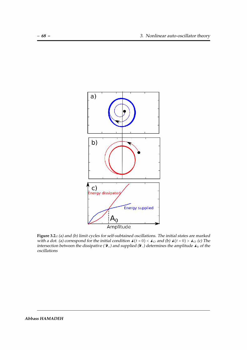
– 68 – 3. Nonlinear auto-oscillator theory
Figure 3.2.: (a) and (b) limit cycles for self-subtained oscillations. The initial states are markedwith a dot. (a) correspond for the initial condition A(t = 0) < AO and (b) A(t = 0) > AO (c) Theintersection between the dissipative ( Γ+) and supplied (Γ−) determines the amplitude A0 of theoscillations
Abbass HAMADEH

3.2. Non-linear auto-oscillator model – 69 –
To summarize, in this section we have introduced the notations and basic concepts of anoscillator. We have included the notions of equilibra, dissipation, forcing, self-substained,limit cycle, and phase portrait. Theses notations will be used later.
3.2. Non-linear auto-oscillator model
We present in this section the nonlinear auto-oscillator (NAO) model that is formulatedfrom equation of motion of magnetization which is presented in chapter 1. This modelis based on the classical quasi-Hamiltonian formalism for spin wave [22] and it considerthat only a single mode is excited at the auto-oscillation threshold. A similar approch ofthe case of multi-mode will be discussed in section 3.5.
It can be shown that the dynamics of the dimensionless complex amplitudec (given byc = Mx−iMy
√
2Ms(Ms+Mz)where Ms is the length of the magnetization saturation vector in the
free magnetic layer, andMx, My and Mz , are the projection of this vector on the equilib-rium magnetization direction x, y and z respectively) which describes magnetizationprecession in a STNO, is given by the following universal form:
∂c
∂t+ iω(∣ c ∣2)c + Γ+(∣ c ∣2)c − Γ−(∣ c ∣2)c = 0 . (3.9)
To recall the different terms used in this equation:
• c: the complex amplitude of auto-oscillations with the power and phase are de-noted p= ∣ c ∣2 and φ = arg(c) respectively.
• ω(p): is the resonance frequency.
• Γ+(p): is the damping rate for the energy dissipation.
• Γ−(p): is the effective negative damping introduced into the system by the spin-polarized current.
Synchronization of spin trasnsfer nano-oscillators

– 70 – 3. Nonlinear auto-oscillator theory
For a simple geometry, when the external magnetic field is applied along the normal ofthe free layer, the dependences of the frequency ω(p) and damping rates Γ±(p) on thepower p can be expressed as a first order series expansion:
ω(p) = ω0 +Np (3.10a)
Γ+(p) = ΓG(1 +Qp +Q′p2) (3.10b)
Γ−(p) = σ0I(1 − p) , (3.10c)
where ω0=γ(Hext − 4πMs), N is the coefficient of the nonlinear frequency shift for thenormally magnetized layer given by N = 2ωM = 2πγMs, ΓG = αGω0 (Gilbert damping),Q = 2ωM/ω0 and Q′ = −2ωM/ω0 represent the nonlinearity of the damping.
The form of equation (3.9) makes easy the analysis and the interpretations of the dynam-ics of magnetization. So, we will use this model along the manuscript and we will startby seeking the solution of this equation.
Stationary regime : The solutions of equation 3.9 is given by the form: c = p exp (iφ).Then, we will separate the real and imaginary parts to obtain a system of two equationsfor the power (p) and the phase (φ):
∂p
∂t+ 2[Γ+(p) − Γ−(p)]p = 0 , (3.11)
∂φ
∂t+ ω(p) = 0 . (3.12)
Two stationary solutions (dp/dt = 0) can be obtained from equation 3.11. The firststationary solution corresponds to p = 0 for which the linearization of equation 3.11yields this solution:
∂p
∂t+ 2[Γ+(0) − Γ−(0)]p = 0 . (3.13)
Based on this equation, it’s clear that when Γ+(0) > Γ−(0) , the solution p = 0 is stable.Then, the condition Γ+(0) = Γ−(0) gives the critical current Ith to obtain auto-oscillation.
Abbass HAMADEH

3.2. Non-linear auto-oscillator model – 71 –
From equations 3.10b and 3.10c, the expression of the critical current is given by (seeequation 1.9) :
Ith =ΓGσ0
. (3.14)
In order to establish the second type of stationary solution when p = p0, the dampingterms should cancel exactly at p = p0 such that Γ+(p) = Γ−(p0). This means that theenergy lost by damping (Γ+(p0)) should be compensated by the energy supplied (Γ−(p0))via spin transfer. Using equations 3.10b and 3.10c and with super-criticality ξ = I/Ith,one can obtain the stationary power (p0) for the STNO:
p0 =ξ − 1
ξ +Q . (3.15)
Two different regimes can be defined for the oscillator: the sub-critical regime (I < Ith)for which the system does not oscillate and the supercritical regime ( I > Ith) for whichthe spin torque driven self-sustained oscillations exist. Then, for small power deviationδp = p − p0 , we can get a damping rate Γp = G+ −G−= (ξ − 1)ΓG where (G+ = dΓ+/dpand G− = dΓ−/dp). Morever, from equation 3.15 , it is possible to describe the frequency,damping and spin transfer term as function of the current as follows:
ω = ω0 +Nξ − 1
ξ −Q (3.16a)
Γ−(p) = σ0IQ + 1
ξ +Q (3.16b)
Γ+(p) = ΓGξ(1 +Q)ξ +Q , (3.16c)
Using the expression of the frequency ω, we can also find the relation between the agilityin the current, which is defined by dω/dI and the nonlinearity factor N :
dω
dI= NI
1 +Q(ξ +Q)2
. (3.17)
The non-linear frequency shift coefficient for STNO strongly depends on the direction ofthe external magnetic field and can be negative or positive. It is possible to introduce the
Synchronization of spin trasnsfer nano-oscillators

– 72 – 3. Nonlinear auto-oscillator theory
normalized dimensionless nonlinear frequency shift ν which characterizes the relativeinfluence of frequency shift N in comparison on damping rate and its can given as:
ν = N
Γpp0 , (3.18)
ν >> 1 for STNOs which make them unique compared to other oscillators. The NAOmodel has many advantages, because it has transformed the LLGS equation into a onesimple equation. So, now we can describe the autonomous regime (i.e: the expressionof frequency, damping, ...). In the next section, we will describe the influence of thethermal noise in the NAO model which leads to an amplitude and phase fluctuationconsequence to linewidth broadening.
3.3. The noise in the NAO Theory
Beside describing the NAO model without external source in section 3.2 , a theory ofnon-autonomous dynamics of a STNO in the presence of thermal noise was developed.This theory is based on the nonlinear oscillator equation for the complex amplitude c(t)of a spin wave exited by spin current. When a force f(t) acts on the STNO, equation 3.9becomes:
∂c
∂t+ iω(∣ c ∣2)c + Γ+(∣ c ∣2)c − Γ−(∣ c ∣2)c = f(t) . (3.19)
It should be noted here that when f(t) is due to a periodic external source, the modeldescribes the synchronization or modulation [90] of STNO to an external source and wewill present this formalism later. In the case of the action of thermal noise, the functionf(t) is a stochastic force. Before we discuss the contribution of phase and amplitudefluctuations to the emitted power and generation linewidth, we will first discuss theorigin of these fluctuations.
3.3.1. Amplitude and phase fluctuations
Due to the small size of an STNO, the thermal fluctuations acting along the trajectoryof the oscillation, cause a spread in the time it takes to complete every orbit by making
Abbass HAMADEH
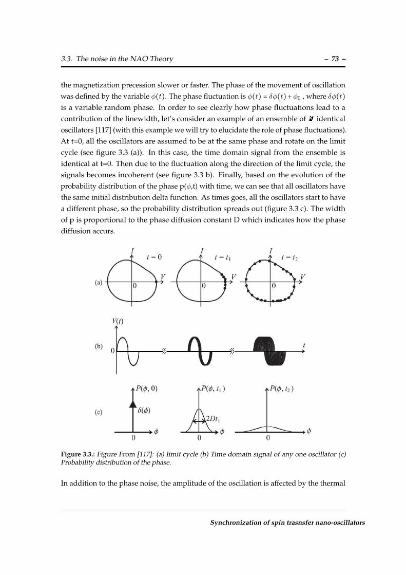
3.3. The noise in the NAO Theory – 73 –
the magnetization precession slower or faster. The phase of the movement of oscillationwas defined by the variable φ(t). The phase fluctuation is φ(t) = δφ(t)+φ0 , where δφ(t)is a variable random phase. In order to see clearly how phase fluctuations lead to acontribution of the linewidth, let’s consider an example of an ensemble of N identicaloscillators [117] (with this example we will try to elucidate the role of phase fluctuations).At t=0, all the oscillators are assumed to be at the same phase and rotate on the limitcycle (see figure 3.3 (a)). In this case, the time domain signal from the ensemble isidentical at t=0. Then due to the fluctuation along the direction of the limit cycle, thesignals becomes incoherent (see figure 3.3 b). Finally, based on the evolution of theprobability distribution of the phase p(φ,t) with time, we can see that all oscillators havethe same initial distribution delta function. As times goes, all the oscillators start to havea different phase, so the probability distribution spreads out (figure 3.3 c). The widthof p is proportional to the phase diffusion constant D which indicates how the phasediffusion accurs.
Figure 3.3.: Figure From [117]: (a) limit cycle (b) Time domain signal of any one oscillator (c)Probability distribution of the phase.
In addition to the phase noise, the amplitude of the oscillation is affected by the thermal
Synchronization of spin trasnsfer nano-oscillators

– 74 – 3. Nonlinear auto-oscillator theory
fluctuation. Here the later act perpendicular to the trajectory of the oscillation whichlead to a fluctuation on amplitude.
3.3.2. Power generated by a STNO
We have presented in details the meaning of amplitude and phase fluctuation. Nowthe goal is to solve equation 3.19 in order to derive the expression of the microwavepower generated by the STNO in the presence of thermal noise. For this purpose wecan consider that the function f(t) which describes the noise caused by temperature is astochastic white Gaussian process [118] with the correlator:
⟨f(t)f∗(t′)⟩ = 2D(p)δ(t − t′) , (3.20)
Where D(p) = Γ+(p)η(p) is the diffusion coefficient constant that characterizes the noiseamplitude of the oscillator with power p, η(p) = γkBT /VeffM0ω(p) is the effectivenoise power which depends on the effective volume Veff of the ferromagnetic materialinvolved in the oscillation. Note that equation 3.19 is nonlinear and stochastic andthus, this equation is difficult to solve. After writing the corresponding Fokker-Planckequation, we come down to a linear and deterministic problem, consequently simpleto solve. The system is described by a function P(t, p, φ) which gives the probability offinding the system with state (p, φ) at time t. The function that describes the system 3.19is a solution of [119] :
∂P∂t
= ∂
∂p[2p(Γ+ − Γ−)P] + ω
∂P∂φ
+ ∂
∂p(2pD
∂P∂p
) + ∂
∂φ(D
2p
∂P∂φ
) . (3.21)
To calculate the power in the presence of thermal fluctuations, we can limit to thestationary case. The stationary solution is independent of the phase φ. Now, we providethe analytic expression of the power distribution going from thermal equilibrium asfollows:
P0(p) = N0exp [−∫p
0(Γ+(p′) − Γ−(p′)
D(p′) )dp′] . (3.22)
Abbass HAMADEH
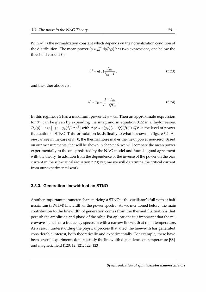
3.3. The noise in the NAO Theory – 75 –
With N0 is the normalization constant which depends on the normalization condition ofthe distribution. The mean power (p = ∫ ∞0 dpP0p) has two expressions, one below thethreshold current Ith:
p< = η(0) IthIth − I
, (3.23)
and the other above Ith:
p> = p0 =I − IthI −QIth
. (3.24)
In this regime, P0 has a maximum power at p = p0. Then an approximate expressionfor P0 can be given by expanding the integrand in equation 3.22 in a Taylor series,P0(p) ∼ exp [−(p − p0)2/2∆p2] with ∆p2 = η(p0)(1 +Q)ξ/(ξ +Q)2 is the level of powerfluctuation of STNO. This formulation leads finally to what is shown in figure 3.4. Asone can see in the case of ξ =0, the thermal noise makes the mean power non-zero. Basedon our measurements, that will be shown in chapter 6, we will compare the mean powerexperimentally to the one predicted by the NAO model and found a good agreementwith the theory. In addition from the dependence of the inverse of the power on the biascurrent in the sub-critical (equation 3.23) regime we will determine the critical currentfrom our experimental work.
3.3.3. Generation linewidth of an STNO
Another important parameter characterizing a STNO is the oscillator’s full with at halfmaximum (FWHM) linewidth of the power spectra. As we mentioned before, the maincontribution to the linewidth of generation comes from the thermal fluctuations thatperturb the amplitude and phase of the orbit. For aplications it is important that the mi-crowave signal has a frequency spectrum with a narrow linewidth at room temperature.As a result, understanding the physical process that affect the linewidth has generatedconsiderable interest, both theoretically and experimentally. For example, there havebeen several experiments done to study the linewidth dependence on temperature [88]and magnetic field [120, 12, 121, 122, 123]
Synchronization of spin trasnsfer nano-oscillators
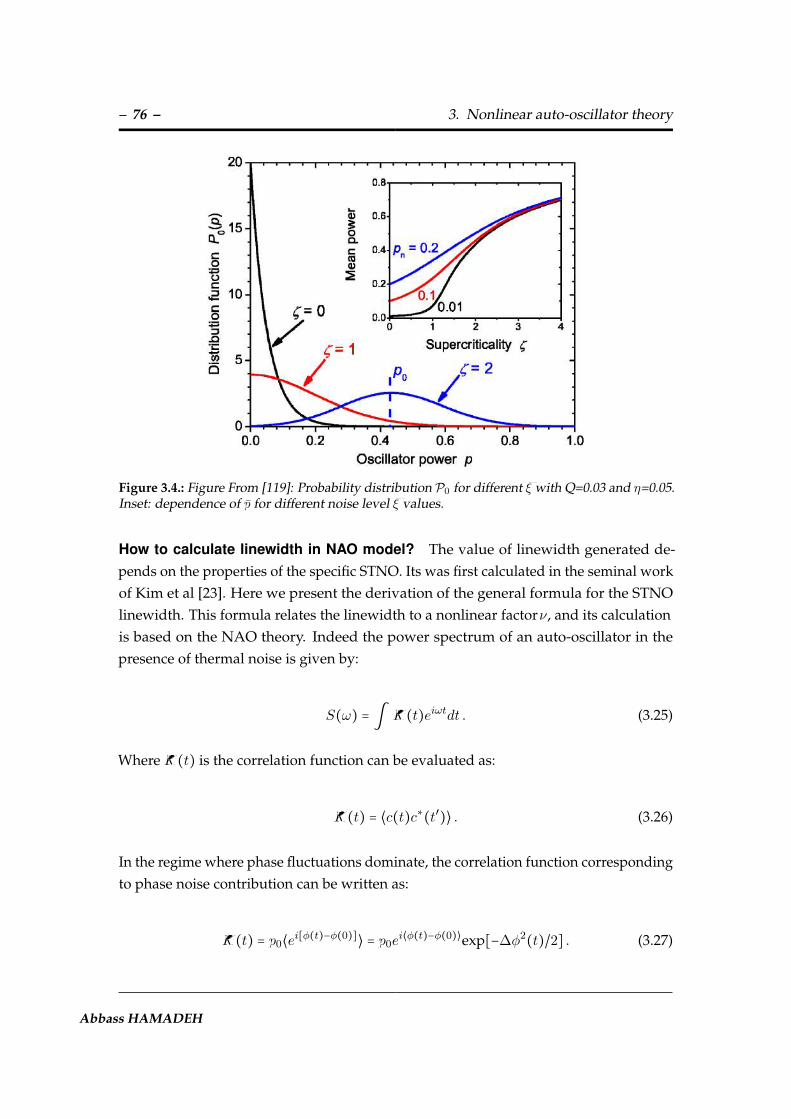
– 76 – 3. Nonlinear auto-oscillator theory
Figure 3.4.: Figure From [119]: Probability distribution P0 for different ξ with Q=0.03 and η=0.05.Inset: dependence of p for different noise level ξ values.
How to calculate linewidth in NAO model? The value of linewidth generated de-pends on the properties of the specific STNO. Its was first calculated in the seminal workof Kim et al [23]. Here we present the derivation of the general formula for the STNOlinewidth. This formula relates the linewidth to a nonlinear factorν, and its calculationis based on the NAO theory. Indeed the power spectrum of an auto-oscillator in thepresence of thermal noise is given by:
S(ω) = ∫ K(t)eiωtdt . (3.25)
Where K(t) is the correlation function can be evaluated as:
K(t) = ⟨c(t)c∗(t′)⟩ . (3.26)
In the regime where phase fluctuations dominate, the correlation function correspondingto phase noise contribution can be written as:
K(t) = p0⟨ei[φ(t)−φ(0)]⟩ = p0ei⟨φ(t)−φ(0)⟩exp[−∆φ2(t)/2] . (3.27)
Abbass HAMADEH

3.3. The noise in the NAO Theory – 77 –
Where ∆φ2(t) is the phase variance and in the case of a nonlinear (or non-isochronous)auto-oscillator its given by:
∆φ2(t) = ⟨φ2(t)⟩ − [⟨φ(t)⟩]2 = 2π∆F0 [(1 + ν2)t + ν2 1 − e−2Γpt
2Γp] , (3.28)
where ∆F0 is the linewidth of the main frequency in an linear (or isochronous) 1 auto-oscillator (in the absence of frequency nonlinearity). ∆F0 = kBT
Es
Γ+2π where kB is the
Boltzmann constant, T is the temperature, Es is the energy stored in the auto-oscillationand Γ+ is the natural energy dissipation rate. Now from equation 3.28 it is possibleto calculate the linewidth of the non-linear auto-oscillator in two different regimes,depending on temperature T , the generation linewidth ∆ω and the the amplitudefluctuations Γp:
• ∆ω << Γp : in this case the exponential factor in the variance (equation 3.28) canbe neglected, then the linewidth becomes:
∆F = kBTEs
Γ+2π
(1 + ν2) , (3.29)
• ∆ω >> Γp in this case the exponential factor in the variance (equation 3.28) can bedeveloped into Taylor series, then the linewidth becomes:
∆F = ∣ ν ∣2π
√Γ+ΓP
√kBT
Es. (3.30)
It is clear that the linewidth scales with temperature and nonlinearity, as the temperatureincreases, the ratio of the noise energy increases leading to increase of linewidth. Inparticular, one can see in expression 7.4 that the nonlinear frequency shift coefficientν, leads to the increase of the linewidth by factor of (1 + ν2). For linear auto-oscillator,where ν = 0, this increase is negligible. In this thesis we will use the first approximateexpression for the non-linear auto-oscillator linewidth, since ∆ω << Γp in our oscillator.Moreover, the nanoscale size of STNOs, although it confers to these devices high agility,broadens substantially the spectral purity since the linewidth depends inversely on
1In an isochronous auto-oscillator, the auto-oscillation frequency f does not depend on the oscillationamplitude.
Synchronization of spin trasnsfer nano-oscillators

– 78 – 3. Nonlinear auto-oscillator theory
Es, which is proportionnal to the sample volume. This is an intrinisc compromise.Synchronization provides a mean to improve the spectral purity by increasing Es.
3.4. Phase-locking and mutual synchronization
A formalism for STNO in terms of nonlinear dynamical equation in the presence ofexternal source or by synchronizing two STNOs were also described within the NAOmodel. In this section we summarize results from literature that used the NAO theory inorder to provide the experimental results in phase-locking and synchronizing STNOs.
Phase-locking to an external source
We mention here the injection locking experiments of STNOs to an external signal.Indeed, these experiments are described by the NAO model where in the equation 3.19,f(t) is a term represents an external harmonic signal (f(t) = fsourcee−iωsourcet). Startingfrom this equation, and following Adler’s formalism [124], it is possible to calculatedthe relevant uniformly rotating phase for the auto-oscillator Φ, that depends on thenon-linearity ν (Φ = Φ − ν δp
2p0), to end up with the equation driving the phase dynamics
of the spin transfer oscillator in the presence of noise:
∂Φ
∂t+ ωoscillator = −
√1 + ν2 ∣ fsource ∣√
p0sin (ωsourcet + Φ − ψsource + arctan(ν)) . (3.31)
Where Φ is the phase difference between the oscillator and the source, ∣ fsource ∣ is thereal amplitude of the external source, and ψsource = arg(fsource) is the initial phase of theexternal source. The oscillator is synchronized if Φ is constant. Then the phase-lockingbandwidth ∆ is given by [97]:
∆ =√
1 + ν2∣ fsource ∣√
p0. (3.32)
One can see, that the nonlinearity of the STNO leads to the increases of the phase-lockingrange by (
√1 + ν2) times. We note here that the nonlinearity isn’t required to phase
Abbass HAMADEH
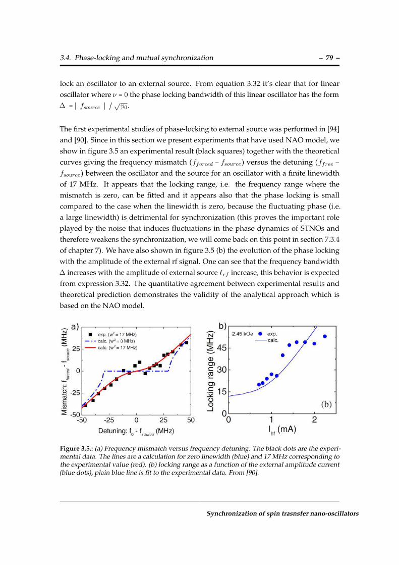
3.4. Phase-locking and mutual synchronization – 79 –
lock an oscillator to an external source. From equation 3.32 it’s clear that for linearoscillator where ν = 0 the phase locking bandwidth of this linear oscillator has the form∆ = ∣ fsource ∣ / √
p0.
The first experimental studies of phase-locking to external source was performed in [94]and [90]. Since in this section we present experiments that have used NAO model, weshow in figure 3.5 an experimental result (black squares) together with the theoreticalcurves giving the frequency mismatch (fforced − fsource) versus the detuning (ffree −fsource) between the oscillator and the source for an oscillator with a finite linewidthof 17 MHz. It appears that the locking range, i.e. the frequency range where themismatch is zero, can be fitted and it appears also that the phase locking is smallcompared to the case when the linewidth is zero, because the fluctuating phase (i.e.a large linewidth) is detrimental for synchronization (this proves the important roleplayed by the noise that induces fluctuations in the phase dynamics of STNOs andtherefore weakens the synchronization, we will come back on this point in section 7.3.4of chapter 7). We have also shown in figure 3.5 (b) the evolution of the phase lockingwith the amplitude of the external rf signal. One can see that the frequency bandwidth∆ increases with the amplitude of external source Irf increase, this behavior is expectedfrom expression 3.32. The quantitative agreement between experimental results andtheoretical prediction demonstrates the validity of the analytical approach which isbased on the NAO model.
Figure 3.5.: (a) Frequency mismatch versus frequency detuning. The black dots are the experi-mental data. The lines are a calculation for zero linewidth (blue) and 17 MHz corresponding tothe experimental value (red). (b) locking range as a function of the external amplitude current(blue dots), plain blue line is fit to the experimental data. From [90].
Synchronization of spin trasnsfer nano-oscillators

– 80 – 3. Nonlinear auto-oscillator theory
Another example of experimental results to be mentioned is the injection locking experi-ment by Bonetti [125] where the locking range has been measured as a function of outof plane magnetic field angle in nano-contact STNOs geometries. It was shown in thiswork that the angular dependence of the locking strength (or phase locking interval),can be explained by using the NAO model. Indeed, as already mentionned in section3.2 that the nonlinear frequency N for STNO strongly depends on the direction of theexternal magnetic field (see figure 6.1 of chapter 6). Since ν = N/(G+ −G−) then, it isunderstandable why the phase locking range ∆ depends on the magnetization fieldangle of the oscillation layer (see figure 3.6).
Figure 3.6.: locking range versus out of plane field angle. the dots represented the experimentalData. The lines are calculated from the NAO model. The dependence of the locking range versusthe out of plane field angle is explained by the variation of the nonlinear frequency shift N withthe external magnetic field. From [125]
Mutual synchronization of two oscillators
Besides injection locking experiments to an external source, the spin-wave formalismof the NAO theory explains as well the mutual synchronization. Indeed, the equationsfor the complex precession amplitudes cj (j = 1,2) in two generating coupling STNOs
Abbass HAMADEH

3.4. Phase-locking and mutual synchronization – 81 –
Figure 3.7.: (a) Power spectra observed when increasing the bias DC current to the structurecomposed of two nano-contacts [28]. (b) Theoretical model which use the NAO theory from[126]
can be written using the formalism of equation 3.9 by introducing a coupling factor Ωj,k
such that [126]:
∂cj
∂t+ iωj(∣ cj ∣2)cj + Γ+(∣ cj ∣2)cj − Γ−(∣ cj ∣2)cj = Ωj,ke
iβj,kck . (3.33)
Where Ωj,k describe the strength of the coupling between the oscillators, and βj,k describethe coupling phases between the jth and kth oscillator. Theses quantities depend onseveral parameters according to the nature of the coupling between oscillator. Forexample, they depend on the distance between the oscillators, and on the orientation,amplitude of the external magnetic field in the case of dipolar coupling.
In particular, it was predicted theoretically that the locking range ∆syn for two identicaloscillators with different frequencies depends on the nonlinearity of the oscillators ν andon the coupling phase β as [22]:
∆syn = 2Ω√
1 + ν2 ∣ cos(β − arctan(ν)) ∣ . (3.34)
For comparison to the theoretical model with experiment, figure 3.7 (a) shows an exam-ple of the mutual phase-locking of two spin-torque oscillators and figure 3.7 (b) showsthe solution of the theoretical equation 3.33. It is clear, that the oscillator mutual synchro-nization theory gives a reasonably good qualitative description of the experiment.
Synchronization of spin trasnsfer nano-oscillators

– 82 – 3. Nonlinear auto-oscillator theory
3.5. Multi-mode oscillator
Usually, only one spin wave mode is excited by the spin-polarized current in STNO 2.Then the NAO model describe several experiments among them [12, 111, 87, 90, 28,27, 42, 123]. However, recent experiments have shown STNOs multi-mode generation[127, 128, 129, 130, 131]. In STNOs exhibiting more than one mode, it is very importantto know if there are interactions between these modes. The distinction between intra-mode coupling (different modes of the same layer) and inter-mode coupling (modesof different layers) can also be significant. This is why a general multi-mode theoryis needed to describe the dynamics in STNO in the presence of two or more modes,and describe the nature and the physical origin of the coupling between theses modes[127, 130, 132, 133, 134, 135]. In nano-contact MTJ STNO, Muduli et al. [128] haveshown that the mode generated by this device can exhibit jumbs between two andthree frequencies when either current or temperature is varied. By extending the NAOtheory, and taking into account the action of thermal noise, Slobodianiuk et al. [135]have shown that two-mode generation is possible to be described analytically. Indeed,we have already mentioned that the magnetization dynamics in STNO’s of a single spinwave mode excited by the bias current can be described by the dimensionless complex cwhich related to the mode power. Now fordouble mode, the equation of motion for theamplitude ci (i = 0,1), whereby the thermal noise is taken into account can be describedas:
∂c0∂t
+ iω0(c0, c1)c0 + Γ0(c0, c1)c0 = f0(t) (3.35a)
∂c1∂t
+ iω1(c0, c1)c1 + Γ1(c0, c1)c1 = f1(t) . (3.35b)
Where the frequency ωi and the action of the spin-polarized current Γi = Γ+i − Γ−i arenonlinear functions of the spin wave power pi. fi(t) is the random white Gaussianprocess that describes the influence of the thermal noise.
2This effect is a direct consequence of the nature of the STT process, which is stimulated emission.Stimulated emission efficiency is proportionnal to magnon occupation of a particular eigen-mode. Thusthe first mode that goes unstable has the highest probability to couple to the dc source of angularmomentum in the STT process. This is similar to the process that leads to laser.
Abbass HAMADEH

3.5. Multi-mode oscillator – 83 –
Then the mean-mode generation power pi is calculated as (see [135] for detailed calcula-tion):
p0 = ∫∞
0∫
∞
0p0P(p0, p1)dp0dp1 (3.36a)
p1 = ∫∞
0∫
∞
0p1P(p0, p1)dp0dp1 . (3.36b)
Where P(p0, p2) is the probability distribution function. The results of calculationsperformed using equations 3.36b are presented in figure 3.8. Here the integrals arecalculated numerically for a value of χ (constant proportional to the temperature inthe system) of 0.2 and 1.2. As one can see, in the case of χ = 0.2 which correspond toa small power of thermal noise, the dependence of the mean power mode c0 versussupercriticality ξ does not change compared to the solution without thermal noise (blackdashed line). In this case the second mode power which presented in blue is very small.Then, by increasing χ the thermal noise promotes the oscillation of the second mode.
Figure 3.8.: Dependence of the mean-mode powers dependence on supercriticality ∆. fordifferent amplitude of phase noise. Dashed line corresponds to the one-mode solution. From[135].
Synchronization of spin trasnsfer nano-oscillators

– 84 – 3. Nonlinear auto-oscillator theory
In sum, we have presented in this chapter the main results of a formalism for STNOsin terms of a universal nonlinear dynamical equation. This theory enables to predictall the useful characteristics of STNOs: generation frequency and linewidth, tun-ability, locking range, synchronization properties. Finally, it deserves to be notedthat the validity of the NAO model for the description of a STNO is not limited tothe case of a uniform magnetization precession. The spin wave mode excited in anSTNO can have an arbitrary spatial distribution, and the NAO model can still beused in the vortex state [37, 136].
Abbass HAMADEH
Part II.
Experimental setup and samples
85


CHAPTER 4
High frequency transport and MRFM
This chapter describes the experimental setups used during this thesis to characterizethe STNO samples. The first part presents briefly the key aspects of the SATM (SpectrumAnalyzer Transport Measurement) setup. In the second part a brief description of theMRFM (Magnetic Resonance Force Microscopy) instrument will be given.
87

– 88 – 4. High frequency transport and MRFM
4.1. Transport measurement
A natural mean to study STNOs is to use their magneto-resistance properties. Indeed,the resistance of a GMR junction depends on the relative angle between the two layers.Then when steady-state oscillations occur, it will generate an oscillating voltage. Thefirst direct measurements of the high-frequency oscillations were undertaken at Cornelland the measurement technique is presented also in the same paper [11]. In this thesis,we measure the spectra of microwave power that result from magnetic motions by usingSATM (Spectrum Analyzer Transport Measurement) technique. A schematic of thistechnique is shown in figure 4.1. In this approach, a DC current is injected throughthe magneto-resistive device to excite the precession of magnetization and because ofthe GMR effect, there is an oscillation change in resistance and then, a time varyingvoltage.
In this setup the sample is mounted on a support between the poles of an electromagnet(cooled down by water) with its power supply to apply a magnetic field up to 1.1 T.The contact to the sample is realized by means of GGB industries microwave probes,with 150 µm pitch and with nominal maximum operating frequency of 20 GHz andnominal impedance Zc = 50 Ω. The probes were custom built in all-non-magnetic parts,in order to avoid movements induced by the external magnetic field generated by theelectromagnet. After the probe, a coaxial cables adapted to high frequency are used withSMA connectors for the connection between the probe and a bias-tee which allows theinjection of AC and DC into the sample simultaneously. Since the determination of thestatic magnetic configuration is based on the measurement of giant magnetoresistanceeffect, an experimental access to the resistance of the device is necessary. For thispurpose, the sample is connected to a dc current source and to a voltmeter through thesame contact electrodes, which can be used for standard current perpendicular to theplane (CPP-GMR) transport measurements. The AC part of the voltage produced bythe sample is sent through a low-noise amplifier having gain + 30 dBm to an AgilentSpectrum Analyzer (SA) with a working range of [9 KHz - 26 GHz] for frequency domainanalysis.
In order to detect voltage oscillations, the relative orientation of the static magnetizationsof the two layers constituting in our spin-valve have to be misaligned in order for themagnetization precession to produce a voltage, because highly symmetric magnetizationtrajectories do not produce any variation of resistance with time.
Abbass HAMADEH

4.2. Magnetic Resonance Force Microscopy – 89 –
Figure 4.1.: Experimental setup spectrum analyzer transport measurement (SATM) for electricalmeasurement. A DC current is applied to the STNO. A bias-tee allows the AC component ofthe current to be extracted, which is then amplified and has measured with an SA. Here thefield is applied by an electromagnet which control the local field on the STNO. In addition thissetup allows monitoring the DC voltage produced across the nanopillar when it is excited by anexternal source. A lock-in amplifier (not shown here) is used in these voltage-FMR measurements.Inset: schematics of an equivalent circuit to the setup.
In our experimental setup it is also possible to monitor the dc voltage produced acrossthe nanopillar by the precession of the magnetization in the sample structure when a rfcurrent is injected in this structure (voltage-FMR). To do this, a lock-in detection is usedto measure the difference of voltage across the nanopillar when the rf is turned ON andOFF: Vdc = VON − VOFF .
4.2. Magnetic Resonance Force Microscopy
In addition to the SATM technique, we will use another independent method of detectingthe magnetic resonance inside our device. We decided to use a mechanical detectionof the FMR with a ferromagnetic resonance force microscope (MRFM)[59], which wasconstructed in the laboratory. This method has several advantages:
• A first decisive advantage is that the detection scheme does not rely on the spinwave spatial symmetry because it measures the change of the static component
Synchronization of spin trasnsfer nano-oscillators

– 90 – 4. High frequency transport and MRFM
(time average) of the magnetization (i.e the component along the precession axisor longitudinal component).
• A second decisive advantage is that the dipolar coupling used in MRFM permitsthe study of buried objects. Importantly, the dynamics of the thin layer underneaththe top contact electrode can be studied.
• A third decisive advantage is that in MRFM, a quantitative measurement of∆Mz ,can be obtained. Thus one can obtain the power of the signal emitted by the STNO(p=∆Mz/2Ms).
4.2.1. Introdution
The dynamics of magnetization in ferromagnetic bodies can be studied using a varietyof different experimental techniques. Among them, Brillouin light scattering (BLS)[137,138], time-resolved scanning Kerr microscopy (TRSKM)[139], X-ray magnetic circulardichroism (XMCD) transmission microscopy [55] and spin-torque driven ferromagneticResonance (ST-FMR)[15, 140].
Magnetic Resonance Force Microscopy (MRFM)[141, 57, 142, 143, 144, 145, 49, 102]which was used in this work, is a powerful technique that can detect any change inthe magnetization of a ferromagnetic sample. This technique was proposed in 1991 bySidles who was searching for a precise technique of measurement to study the structureof biological objects and to achieve this goal he came up with the intriguing idea whichis to couple a highly sensitive force detector like a micrometer sized cantilever to thelongitudinal component of magnetic moment of either nuclear or electronic spins. Thecapabilities of the MRFM to detect the electron spin resonance (ESR) was given byRugar team (1992) in the DiphenylPicrylhydrazyl (DPPH) molecule [146], the nuclearmagnetic resonance (NMR) [147], ferromagnetic resonance (FMR) experiments [56]. Inthe following section, we will give a brief overview of our MRFM experiment.
4.2.2. MRFM operating principles
The principles of MRFM are the same as that of the magnetic force microscope (MFM)technique, which measures the magnetic interaction between the probe and the sample.In fact, when a magnetic moment m is placed in a gradient field ∇B, it will experience a
Abbass HAMADEH
4.2. Magnetic Resonance Force Microscopy – 91 –
force F = (m.∇)B. In MRFM, the gradient B is supplied by a very small probe magnetor ferromagnetic nano-particle mounted at the end of a very soft mechanical resonator(cantilever) and the momentm is produced by the spins of the sample. For an orientationof the external magnetic fields (produced by an electromagnet) along the unit vector zand the cantilever shown in figure 4.2 the force on the cantilever is :
Fz = (mz.∇)Bz . (4.1)
Here the cantilever can detect the force in the z direction only, i.e, the forces in the x andy direction are neglected. Indeed, the mechanical oscillator (cantilever and probe) isnot sensitive to the rapid oscillation of the transverse component in the sample, whichoccurs at the Larmor precession frequency. As a result, the force on the cantilever probeis proportional to the static component of the magnetization inside the sample whichis equal to Mz. When a resonance is excited in the sample, it opens up a precessionmovement at a cone angle θ, it is the deviation of static magnetization Mz from Ms,∆Mz =Ms−Mz =Ms(1−cos(θ)), that leads to changes of the force acting on the cantilever.This force is measured through the detection of the oscillation amplitude of the cantileverusing a laser beam on a four-quadrants photodiode. Here the detection noise is ultimatelylimited by the Brownian motion of the cantilever. This noise depends on the temperatureT and the detection bandwidth B, as well as mechanical characteristics of the harmonicoscillator (resonator) like quality factor Q, spring constant k and mechanical resonancefrequency of the first flexural mode of the cantilever fc. Thus the minimal detectableforce follows the relation:
Fmin =√
4kBTB
ωcQ. (4.2)
In order to obtain a sensitivity gain, the dynamics of the magnetic moments are excitedat fc. This is achieved by the modulation of the microwave excitation at this frequency.As a result, the amplitude of vibration will be multiplied by Q, the quality factor of themechanical resonator.
Synchronization of spin trasnsfer nano-oscillators

– 92 – 4. High frequency transport and MRFM
Figure 4.2.: A schematic of a MRFM apparatus : the electromagnet (not shown) provides anexternal fieldHext perpendicular to the cantilever axis. A small probe magnet is attached at theend of cantilever and is coupled dipolarly to the sample placed underneath. The excitation comesfrom a microwave strip-line placed underneath the sample which produces an RF modulationfield. The displacement of the cantilever is measured optically. Image taken from [59].
4.2.3. Experimental realization
Figure 4.3 displays our MRFM in graph and computer design drawing. The system isset between the poles of an electromagnet which produces an external magnetic field(Hext) oriented out of plane i.e. along the sample axis. This electromagnet can reach1.1 T at room temperature. In our setup it’s very important to set the alignment ofour MRFM cantilever because the later has to be brought into close proximity of thesample in order to maximize the dipolar interaction. For this purpose, we first manuallyalign the cantilever to within a few micrometers. Then, we mount the experiment in avacuum chamber (10−6 mbar) in order to achieve the detection sensitivity. At this stage,the cantilever isn’t placed exactly over the sample. Thus, for the fine alignment, thesample is placed on a piezoelectric tube (see figure 4.3 (c)). The tube has a nanometeraccuracy and can be distorted in a sufficiently large range (micrometer range) in thethree dimension (XYZ). This positioning system is driven by applying high voltage onits electrodes. Then, for positioning the magnetic probe precisely above the center of the
Abbass HAMADEH

4.2. Magnetic Resonance Force Microscopy – 93 –
sample, we search for the minimum of the cantilever frequency which corresponds tothe maximum dipolar interaction between the sample and the probe [61].
Synchronization of spin trasnsfer nano-oscillators
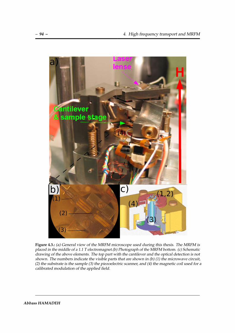
– 94 – 4. High frequency transport and MRFM
Figure 4.3.: (a) General view of the MRFM microscope used during this thesis. The MRFM isplaced in the middle of a 1.1 T electromagnet.(b) Photograph of the MRFM bottom. (c) Schematicdrawing of the above elements. The top part with the cantilever and the optical detection is notshown. The numbers indicate the visible parts that are shown in (b) (1) the microwave circuit,(2) the substrate is the sample (3) the piezoelectric scanner, and (4) the magnetic coil used for acalibrated modulation of the applied field.
Abbass HAMADEH
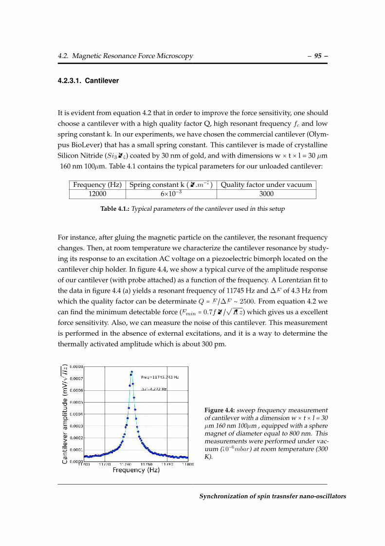
4.2. Magnetic Resonance Force Microscopy – 95 –
4.2.3.1. Cantilever
It is evident from equation 4.2 that in order to improve the force sensitivity, one shouldchoose a cantilever with a high quality factor Q, high resonant frequency fc and lowspring constant k. In our experiments, we have chosen the commercial cantilever (Olym-pus BioLever) that has a small spring constant. This cantilever is made of crystallineSilicon Nitride (Si3N4) coated by 30 nm of gold, and with dimensions w × t × l = 30 µm160 nm 100µm. Table 4.1 contains the typical parameters for our unloaded cantilever:
Frequency (Hz) Spring constant k (N.m−1) Quality factor under vacuum12000 6×10⁻³ 3000
Table 4.1.: Typical parameters of the cantilever used in this setup
For instance, after gluing the magnetic particle on the cantilever, the resonant frequencychanges. Then, at room temperature we characterize the cantilever resonance by study-ing its response to an excitation AC voltage on a piezoelectric bimorph located on thecantilever chip holder. In figure 4.4, we show a typical curve of the amplitude responseof our cantilever (with probe attached) as a function of the frequency. A Lorentzian fit tothe data in figure 4.4 (a) yields a resonant frequency of 11745 Hz and ∆F of 4.3 Hz fromwhich the quality factor can be determinate Q = F /∆F ∼ 2500. From equation 4.2 wecan find the minimum detectable force (Fmin = 0.7fN/
√Hz) which gives us a excellent
force sensitivity. Also, we can measure the noise of this cantilever. This measurementis performed in the absence of external excitations, and it is a way to determine thethermally activated amplitude which is about 300 pm.
Figure 4.4: sweep frequency measurementof cantilever with a dimension w × t × l = 30µm 160 nm 100µm , equipped with a spheremagnet of diameter equal to 800 nm. Thismeasurements were performed under vac-uum (10−6mbar) at room temperature (300K).
Synchronization of spin trasnsfer nano-oscillators

– 96 – 4. High frequency transport and MRFM
4.2.3.2. Probe magnet
Figure 4.5: Scanning electron microscopy im-age of the magnetic probe (FeSi) glued at thetop of a BioLever cantilever.
We have already mentioned in equation 4.1 that the force is created if the magneticmoments of the sample interact with a field gradient. In order to increase the probe-sample interaction and hence MRFM sensitivity we need to increase the magnetic fieldgradient of the probe. In our case, the probe itself is an 800 nm diameter sphere ofamorphous Fe (with 3 % Si) glued at the apex of the cantilever (see figure 4.5). Thechoice of the spherical shape, small size and the material for the magnetic probe is due toseveral reasons. First, the spherical shape preserves the axial symmetry of the nano-pillarand this geometry does not has any shape anisotropy 1 which decreases the influenceof the applied magnetic field on the mechanical resonance frequency of the cantilever.Secondly, a small probe magnet provides larger magnetic field gradient. Finally, FeSiwas chosen to provide a high magnetization Ms to maximize the field gradient.
To characterize this sphere, we have performed a magnetometry measurement by mea-suring the cantilever frequency fc as a function of the applied magnetic field. In thisexperiment the magnetic probe is placed 13µm above the center of a magnetic cylinderwhich produces a known source of field gradient. The resulting cantilever frequencyis shifted due to the presence of the magnetic moment and can be obtained with thefollowing equation:
∆fc
fc= −m
2k(∂
2Bz∂z2
)z0
, (4.3)
where z0 is the equilibrium position of the nanomagnet in the field gradient. The experi-
1The shape anisotropy could induce parasitic torques which can disturb the motion of the cantilever.
Abbass HAMADEH

4.2. Magnetic Resonance Force Microscopy – 97 –
Figure 4.6: The cantilever frequency asa function of the applied magnetic fieldin a field gradient of ∂
2Bz
∂z2= 109G/cm2.
ment shows a linear dependence of the frequency shift with the particle magnetization,since it has a change of the slope at 0.65 T which indicates the magnetic saturation of theprobe. We have indicated in table 4.2 the final extracted values of the radius R, magneticmoment m, and saturation magnetization Ms of the (FeSi) probe with the experimentalerror bars.
Radius (nm) Magnetic moment (emu) Magnetization (emu/cm3)350 ± 30 (2.8 ± 0.7)×10−10 1550 ± 70
Table 4.2.: Summary of the cantilever magnetometry measurements performed to characterizethe probe on the cantilever [148]
4.2.4. Experimental precision
4.2.4.1. Tip stray field
Exhaustive past studies [144, 59], have already demonstrated that, in the weak perturba-tion regime, the influence of the magnetic probe of the MRFM is mostly reduced to auniform shift to lower field of the whole spectrum of the studied sample by an offsetfield:
Hsphl,n =1
⟨M2⊥(r)⟩ ∫vHsph(r)M2
⊥(r)d2(r)dz . (4.4)
Synchronization of spin trasnsfer nano-oscillators

– 98 – 4. High frequency transport and MRFM
where Hsph is the magnetic stray field generated by the sphere. Although the exactshift value in equation 4.4 depends on the mode index [81], it turns out that within theexperimental precision, this offset can be approximated to a constant [144]. Performinga numerical application for the uniform precession profile , we calculate Hsph0,0 = 180Oe when our magnetic sphere with magnetic moment m = 2.8 ×10⁻¹⁰ emu is set at adistance s = 1.3 µm from the sample (all the MRFM spectra are recorded with magneticsphere at the same exact position above the sample 1.3µm). Notice that another way todirectly measure the value of Hsph can be done by measuring the voltage-FMR detectionwith the sphere above the sample. In this case, it is possible to compare the FMR spectrawith and without the presence of the spherical magnetic probe above the sample. Wefind experimentally that the two spectra are homogeneously shifted from each other,and that the shift Hsph = 190 Oe is in a good agreement with the estimation based onequation 4.4.
4.2.4.2. Calibration of ∆Mz
As we mentioned previously, the MRFM experiment consists of detecting mechanicallythe diminution of spontaneous magnetization in the sample associated with the Larmorprecession. The mechanical oscillator is not sensitive to the rapid oscillations of thetransverse component in the sample, which occurs at the Larmor precession frequency,i.e. several orders of magnitude faster than its mechanical resonance. Thus, the magneti-zation of the sample acting on the cantilever probe reduces to the static componentMz .The measured MRFM quantity is given by :
⟨Mz⟩ ≡1
V∫VMz( r)d3r , (4.5)
where the chevron brackets stand for the spatial average over the volume of the mag-netic body. A calibration of ⟨Mz⟩ is possible by using the same experimental foldoverphenomenon as in the RF calibration. In fact for the special case of a sample magnetizedperpendicular to the plane, the amplitude of the uniform mode is a solution of theoperational foldover equation :
[(2(H −Hres)/∆H + βA2)2 + 1]A2 = 1 . (4.6)
Abbass HAMADEH

4.2. Magnetic Resonance Force Microscopy – 99 –
In equation 4.6, H is the applied static field, Hres is the resonance field at low power,∆H is the linewidth measured in the linear regime, β is a parameter proportional to themicrowave power level and A is the amplitude. MRFM profiles with power = +9 dBm isshown in figure 4.7. The spectra are fitted with equation 4.6. From the parameters ∆H
= 0.1 kOe and Hr= 10.7 kOe we obtain β = 83√
3. Hence, the maximal amplitude of the
resonance, which is equal to the longitudinal change of the magnetization is [149]:
4π⟨∆Mz⟩ =4
3√
3∆H . (4.7)
A numerical application of equation (4.7) yields 4π⟨∆Mz⟩ = 36 ± 4 G, which correspondsto the critical angle of precession ⟨θc⟩ = 5. We have used this calibration of the cantilevervibration amplitude to evaluate the change of the longitudinal magnetization ∆Mz .
Figure 4.7: The resonance curve at dif-ferent microwave power in the non lin-ear regime. The foldover threshold (redcurve) gives a fit of the experimentaldata in order to give a direct calibrationof the measured amplitude.
Synchronization of spin trasnsfer nano-oscillators
– 100 – 4. High frequency transport and MRFM
In this chapter we have presented the experimental techniques that will be used tostudy the STNO samples. Our study will be done by two independent methods ofdetecting the magnetization dynamics inside a spin-valve nano-structure. The firsttool is MRFM, which detects all the excited spin wave modes independently of theirphase. In particular, it allows us to perform a study in the exact normal configuration,which is the simplest possible geometry for a STNO as it coincides with the univer-sal auto-oscillator model. The second tool is the SATM where we detect the voltageproduced across the STNO. It deserves to be mentioned that in the MRFM setup, themagnetization dynamics can also be simultaneously detected via SATM technique.In this case the device electrodes are not directly connected to the microwave synthe-sizer through a picoprobe but are wire bounded to a microwave cable and the circuitcontains more connections. Thus, the MRFM spectra can be directly compared totransport measurements in order to better understand the experimental results.
Abbass HAMADEH

CHAPTER 5
Studied samples
As mentioned previously, the current density required for spin transfer effect is high( ∼ 107A/cm2). As a result, nano-scaled device would require several mA. Thus, nanofab-rication is necessary to make a STNO. This chapter starts with a description of the samplestructure and fabrication , followed by a description of the magnetic properties and DCcaracterization. Then, a precise identification of the spin-wave eigen-modes inside thesample will be given.
101

– 102 – 5. Studied samples
5.1. Nano-pillar structure and sample design
5.1.1. The lithographically patterned nanostructure
The spin-valve structure used in this thesis is a standard Permalloy (Ni80Fe20=Py) bi-layer structure sandwiching a 10 nm copper (Cu) spacer: the thicknesses of the thinPya and the thick Pyb layers are respectively ta = 4 nm and tb = 15 nm. The samples arefabricated in laboratoire de photonique et nanostructures (LPN) and CNRS-Thales. Wepresent in this section the process of the production of these metallic nano-pillars.
We can describe the different steps of the fabrication process as follow (see figure 5.1).
Figure 5.1.: Fabrication processes for the production of a nanopillar
1. Sputtering magnetic layers : the first step in the fabrication process is sputteringthin films of all the layers. The metal stack chosen for the samples studied is stillthe same where the metallic layers were deposited onto oxidized Si substrates:Cu(60nm)/Py(15nm)/Cu(10nm)/Py(4nm)/Au(25nm).
2. Electron-beam lithography : after sputtering all the layers, the nanopillar device is de-fined to be circular with dimension of the order of several hundreds of nanometersby electron-beam lithography. The layer of PMMA resist is used to give a goodundercut.
3. Mask Au/Ti: after developing the e-beam resist, an etching mask Au/Ti is deposited.
Abbass HAMADEH

5.1. Nano-pillar structure and sample design – 103 –
Figure 5.2: Schematic representation of the sam-ple which is a circular nano-pillar comprisinga thin Pya and a thick Pyb magnetic layers sep-arated by a Cu spacer. The inset is a top viewmicroscopy image of the sample showing thetwo independent circuits in different colors. Theelectrodes in blue represent the antenna circuitwhich enables to produce an RF in-plane mag-netic field. The electrodes in red represent thecontact circuit that allow for injecting a DCor/and RF current through the nano-pillar.
4. Lift-off : the resist and the Au/Ti is removed except above the device by lift-off inorder to define the etching mask of the nano-pillar. .
5. Ion beam etching : Then the multilayer is etched as a nano-pillar by Ion BeamEtching (IBE).
6. Isolate devices : In order to isolate the device an insulating SU-8 is deposited tocover the whole pillar.
7. Reactive ion etching and planarization : at this point of the fabrication process, thereis SU-8 above everything on the wafer, the next step involve selectively removingSU-8 above the devices. This is done by Reactive Ion Etching (RIE). Then, thesurface is planarized to flatten the bump above the pillar. This is done using theion-milling technique.
8. Contacting the top : Finally, optical lithography is used to make the contact in thetop of the nanopillar by depositing Au over the top-lead.
In addition, an independent top microwave antenna is deposited , with the aim ofproducing an in-plane rf magnetic field hrf at the nanopillar location. This is followedby two steps :
1. Isolate devices: a polymer layer that provides electrical isolation from the rest of thestructure is deposited.
2. Antenna : Then, a broadband strip-line antenna that consists of a 300-nm-thickAu layer is evaporated on the top. The width of the antenna constriction situatedabove the nanopillar is 10 µm. The microwave antenna circuit is shown in blue infigure 5.2 .
Synchronization of spin trasnsfer nano-oscillators

– 104 – 5. Studied samples
Finally it deserves to be mentioned here that the design of the contact electrodes (topand bottom) is done in a specific form (see red circuit in figure 5.2) to minimize the Oefield created by the current which prevents parasitic torques, which may disturb themotion of the cantilever.
5.1.2. The different samples
In this thesis, two batches of samples were produced. The first batch of devices havingonly single nano-pillar. The STNO in this series is a circular nanopillar of nominaldiameter 200 nm patterned from the stack which is discribed previously. The thicknessesof the two magnetic layers have been chosen in order to observe the effects of spintransfer on both layers. Moreover, the spacer layer, of thickness only 10 mm is thinenough to have a dynamic coupling between the two magnetic layers in dipol interaction. Thus, in these samples which contain only one pillar, we will focus to the dynamics ofmagnetization of the coupled two magnetic layers. We note that, the selected materialPermalloy and the dimensions of each magnetic disks are also with the aim of havingstable uniform and vortex states. Indeed, it will be possible to change on the stability ofdifferent magnetic configurations by applying a current or an external magnetic field.
A second series of samples was prepared for which the electron beam lithographymask was modified to prepare for each sample several nano-pillars. We will study onlysamples that are of pair of spin valve nanopillars, processed using the same steps ofe-beam and UV lithography and the same stack described previously. The structure ofeach pillar is the same as that described previously and the separation distance is 100 nm.The top and bottom electrodes are common to the two pillars. The characterization ofthis sample will be presented in chapter 8.
In this thesis two classes of configurations will be studied, these configurations arecharacterized by different excitation modes and frequency ranges:
• Homogeneous nano-pillar: Here the basic configuration is a circular nanopillarstructure which has been presented previously, with a homogeneous magnetizationfor the thin Pya and the thick Pyb. When the magnetizations of both layers areout-of-plane (a strong perpendicular magnetic fields is applied), the frequency ofthe uniform excitation mode is between 2-25 GHz
Abbass HAMADEH
5.2. The microwave circuit: design and calibration – 105 –
• Vortex nano-pillar: Here in the vortex state, the in-plane magnetization curls alongthe pillar border, leading to a singularity in the center (the vortex core), wherethe magnetization turns out of plane . The dynamics of the vortex state whichis very different from the one of the homogeneous state, since the very narrowregion of the soliton-like vortex core (a few nanometers) leads to very differentunique dynamical modes. The lowest energy mode, excited by spin transfer, isthe gyrotropic mode (frequency range 200 MHz - 2 GHz ) where the vortex core isorbiting on a circular trajectory around its equilibrium position. In this thesis, wewill study the dynamic behavior of vortex when excited in a coupled dynamicsbetween the thick and the thin layers.
5.2. The microwave circuit: design and calibration
The microwave circuit has been designed specially for the MRFM setup. A specialcare has been put in the design of the microwave circuit and the electrodes aroundthe nano-pillar. The circuit is adapted at 50 Ω to minimize the parasitic reflexions.The microwave antenna is close as possible from the samples to get the maximum ofamplitude and to generate homogeneous microwave field. It should be noted thatfor the microwave antenna an anti-node is created at the end which leads to a totalreflexion of the microwave current to the source (Anritsu synthesiser, 100 kHz to 20 GHz).The constriction is 10 µm wide and 25 µm long and creates an orthoradial microwavefield hrf that is linearly polarized. Simulations have been performed with the Sonnetmicrowave software in order to validate the properties of the design of this circuit.
5.2.1. Modulation of the microwave source
The goal of MRFM is to detect ferromagnetic resonance at high frequency. To enable this,a microwave field at these frequencies has to be created in the near field of the sample.For this purpose, two different circuits have been designed to excite the magnetizationdynamics and perform spectroscopy. The figure 5.3 shows the first circuit allowing thegeneration of an rf in-plane magnetic field hrf and the circuit allowing the injection of anrf current perpendicular to the plane through the nanopillar irf . The microwave circuitwas carefully designed to minimize the crosstalk between the RF field and RF currentexcitation parts.
Synchronization of spin trasnsfer nano-oscillators

– 106 – 5. Studied samples
Figure 5.3.: Schematic representation of the differ-ent excitation circuit available in our setup. Threedifferent means are available to put the system outof equilibrium: Firstly an RF magnetic field appliedparallel to the layers (blue arrow) secondly an RFcurrent flowing perpendicularly to the layers (redarrow). Finally a DC current Idc flowing through thenano-pillar.
As discussed in the previous chapter,the DC current can cause steady stateoscillations of the magnetization inthe microwave frequency range. Forthis we will inject a finite DC currentIdc in the sample, and study our de-vice in the two regimes: autonomousregime which corresponds to studythe sample under the action of onlythe DC current and forced regimewhich correspond to study the sam-ple under the action of the DC cur-rent and its response to external per-turbations created by rf circuit. Itis also possible to do spectroscopicstudy where there is no dc currentflowing through the device in orderto identify (excite) the eigen-modes inthe STNO. Finally, we mention thatin all these excitations a source mod-ulation is applied at the cantilever fre-quency in order to get rid of spuriouscontributions and to enhance the sig-nal by increases the quality factor ofthe mechanical oscillator. This modu-lation does not affect the line shape ofthe linear regime, because the relax-ation time of the ferromagnetic sys-tem is very small compared to the period of the modulation 1/fc.
Abbass HAMADEH
5.2. The microwave circuit: design and calibration – 107 –
5.2.2. Calibration of microwave setup
5.2.2.1. Calibration of rf field
The amplitude of the RF magnetic field produced by the microwave antenna can be cali-brated based on intrinsic nonlinear properties of the sample. In fact, it was pointed outby Anderson and Suhl [149] that the resonance curve at high power should be skewed,because the static change of the magnetization Mz , which also shifts the resonancefrequency. This is the foldover phenomenon (see figure 4.7) which is characterized by acritical power, for which the resonance curve becomes infinite on the low field side ofthe resonance:
hc = 2∆H
¿ÁÁÀ 2∆H
3√
3[Nzz − Nxx]4πMs
. (5.1)
Where Nxx and Nzz are the demagnetizing factors in the transverse and longi-tudinal directions respectively. ∆H is the linewidth measured in the linear regime.Experimentally, we find that hrf = 4.2 ± 0.8 Oe for an amplitude power of +9 dBm.
It is also possible to estimate the amplitude of hrf from Maxwell-Ampere law :
hrf =µ0
w
√Prf
2Z. (5.2)
Where Z = 50Ω is the impedance matched to the synthesizer and w is the width of theconstriction. The value estimated by this method is hrf = 5.5 ± 1 Oe for Prf = +9 dBmwhich is a good agreement with the estimation made in equation 5.1.
5.2.2.2. Calibration of rf current
Here we detail the experimental protocol used to calibrate the RF current flowingthrough the device with respect to the synthesizer output power injected into the contactelectrodes. We have first used the voltage-FMR technique, in which the sample electrodesare connected to the microwave synthesizer through a picoprobe to perform voltage-FMR spectroscopy. In this experiment, the amplitude of irf flowing through the samplecan be accurately determined, owing to the determination of losses and reflexions in
Synchronization of spin trasnsfer nano-oscillators

– 108 – 5. Studied samples
the microwave circuit using a network analyzer. Then, the same experiment is repeatedinside the MRFM setup, in which the contact electrodes are wire bounded to a microwavecable and the circuit contains more connections. The comparison with the SATM setupyields an estimation of the rms amplitude of the RF current in the mechanical-FMRsetup: irf = 170 ± 40 µA for an output power of −22 dBm injected at 8.1 GHz through thecontact electrodes.
5.3. The magnetic properties of the sample
First of all, the magnetic properties of the Py layers (thick and thin) have to be de-termined. A precise extraction of the material properties (for the two layers) like thesaturation magnetization, the damping parameter and the effective gyro-magnetic ratioγ are given by by cavity FMR and MRFM measurements. In summary the obtainedvalues of the magnetic parameters are the ones reported in table 5.1. More details aboutthe extraction of these parameters can be found in [41].
Table 5.1.: Fundamental magnetic parameters of the thin Pya and thick Pyb layers measured bycavity-FMR on the reference film (top row) and by MRFM (bottom row) in the p3460 sample
4πMa (G) αa 4πMb (G) αb γ (rad ⋅ s−1 ⋅G−1)
8.2 × 10³ 1.5 × 10⁻² 9.6 × 10³ 0.9 × 10⁻² 1.87 × 10⁷
8.0 × 10³ 1.4 × 10⁻² 9.6 × 10³ 0.85 × 10⁻² 1.87 × 10⁷
5.4. DC and high frequency characterization
5.4.1. DC characterization
To characterize the DC properties of our devices, we have reported in figure 5.4 themeasurement of the GMR in our sample in the CPP geometry (current perpendicular tothe plane). The curve represents the hysteric behavior on the magneto-resistance of thespin valve under an in-plane magnetic field bias. Dark symbols (respectively light) are
Abbass HAMADEH

5.4. DC and high frequency characterization – 109 –
used to show the behavior for sweep down (respectively up) in field. The low and highresistance states correspond to the uniformly magnetized state in both the thin and thethick layers, respectively parallel or anti-parallel to each other. The intermediate stateobserved around zero magnetic field corresponds to the formation of a vortex state inthe thick layer. In our device, the average resistance is about 3.6 Ω and the ∆R = 25mΩ
which corresponds to a GMR ∼ 0.7%.
Figure 5.4.: GMR hysteresis curve of the nano-pillar for in plane magnetic field. The field isswept from positive values to negative (dark symbols) values and back to positive saturation(light symbols). On the left: cartoon of the sample structure.
5.4.2. RF characterization
The goal of our experiment is to study the magnetization dynamics in the STNO, bymeans of the STT effect. For this purpose, we aim to perturb the magnetization equilib-rium with a DC current. The effect of the current was checked firstly by using the SATMtechnique. In figure 5.5 we show the power spectral density acquired for an externalfield Hperp = 0.95 T applied out of plane of the layers with θH = 20. For a fixed negativecurrent corresponds to a flow of electrons from the PyB thick layer to the PyA thin layerand stabilizes the parallel configuration due to the spin transfer effect [6, 7]. This testvalidates that our sample is ready to be studied.
Synchronization of spin trasnsfer nano-oscillators
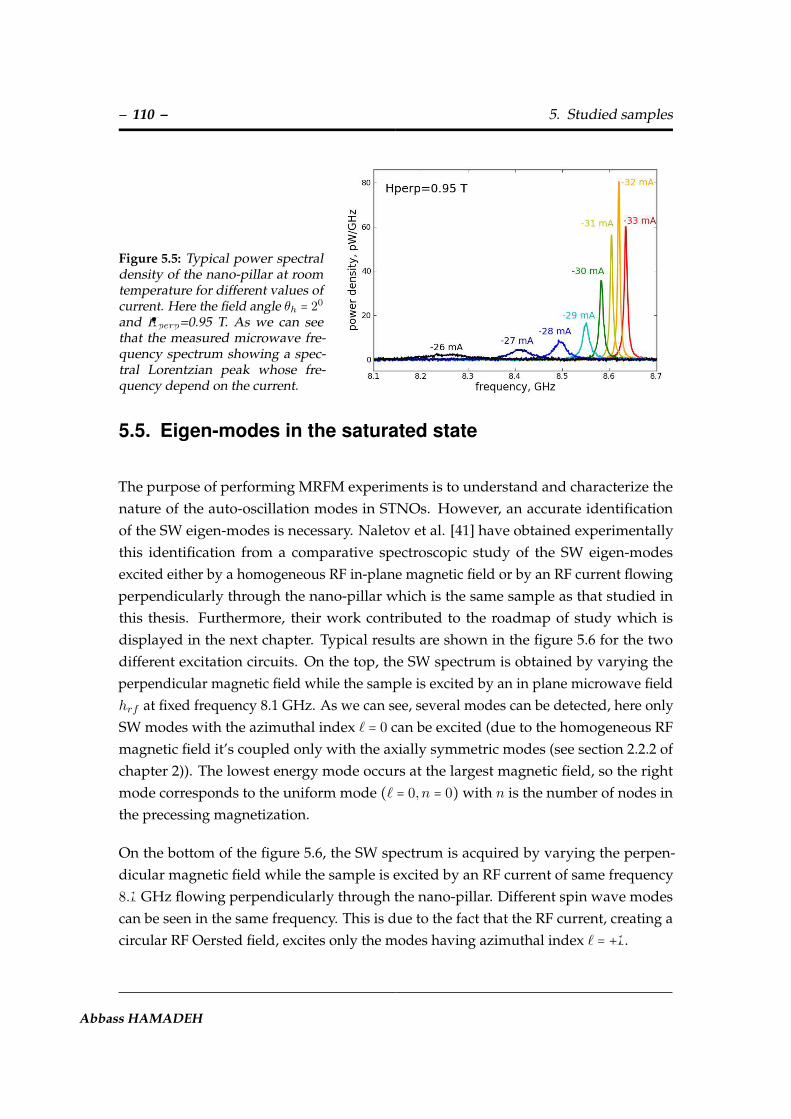
– 110 – 5. Studied samples
Figure 5.5: Typical power spectraldensity of the nano-pillar at roomtemperature for different values ofcurrent. Here the field angle θh = 20
and Hperp=0.95 T. As we can seethat the measured microwave fre-quency spectrum showing a spec-tral Lorentzian peak whose fre-quency depend on the current.
5.5. Eigen-modes in the saturated state
The purpose of performing MRFM experiments is to understand and characterize thenature of the auto-oscillation modes in STNOs. However, an accurate identificationof the SW eigen-modes is necessary. Naletov et al. [41] have obtained experimentallythis identification from a comparative spectroscopic study of the SW eigen-modesexcited either by a homogeneous RF in-plane magnetic field or by an RF current flowingperpendicularly through the nano-pillar which is the same sample as that studied inthis thesis. Furthermore, their work contributed to the roadmap of study which isdisplayed in the next chapter. Typical results are shown in the figure 5.6 for the twodifferent excitation circuits. On the top, the SW spectrum is obtained by varying theperpendicular magnetic field while the sample is excited by an in plane microwave fieldhrf at fixed frequency 8.1 GHz. As we can see, several modes can be detected, here onlySW modes with the azimuthal index ` = 0 can be excited (due to the homogeneous RFmagnetic field it’s coupled only with the axially symmetric modes (see section 2.2.2 ofchapter 2)). The lowest energy mode occurs at the largest magnetic field, so the rightmode corresponds to the uniform mode (` = 0, n = 0) with n is the number of nodes inthe precessing magnetization.
On the bottom of the figure 5.6, the SW spectrum is acquired by varying the perpen-dicular magnetic field while the sample is excited by an RF current of same frequency8.1 GHz flowing perpendicularly through the nano-pillar. Different spin wave modescan be seen in the same frequency. This is due to the fact that the RF current, creating acircular RF Oersted field, excites only the modes having azimuthal index ` = +1.
Abbass HAMADEH

5.5. Eigen-modes in the saturated state – 111 –
Figure 5.6.: Comparative spectroscopic study per-formed by MRFM. (a) and (b) panels show thespin-wave mode spectra excited by a uniform mi-crowave field and a microwave current flowingthrough the nano-pillar, respectively. The posi-tions of the peaks are reported in table 5.2.
Figure 5.7.: Simulated precession patternsof the eigen-vectors. (a) shows the preces-sion profiles across the thin (light color)and thick (dark color) layers. (b) and (c)show the dynamics in the thin Pya andthick Pyb layers, respectively. (see chapter2 for the color code)
In order to identify which layer (thick or thin) contributes mostly to each resonant modea direct current is added through the nano-pillar, because it produces opposite spintransfer torques on each magnetic layers [41]. In addition the experimental results arecompared to theoretical prediction of the nanopillar spin-wave spectra calculated bothanalytically (see section 2.2.2 of chapter 2) and numerically. Figure 5.7 (a) shows therelative amplitudes of precession in each layer to identify the dynamic coupling betweenthe disks. From the profiles shown in figure 5.7, one can then determine which layer (thin Aij or thick Bij) contributes mostly to each dynamic mode. The summary of theprecise identification is presented in table 5.2.
Synchronization of spin trasnsfer nano-oscillators

– 112 – 5. Studied samples
À Á Â Ã10.69 kOe 9.65 kOe 9.51 kOe 8.64 kOe
B00 B01 A00 A01
Ê Ë Ì Í10.22 kOe 9.17 kOe 9.07 kOe 8.22 kOe
B10 B11 A10 A11
Table 5.2.: The resonance field values for the spin wave modes. The blue and red indices arethe location of the SW modes measured experimentally in figure 5.6. Second line representsthe experimental field peaks measured at f=8.1 GHz by sweeping the field. Third refers to theEigen-modes indexed with label j`n where j = A,B indicates the layer (respectively the thin andthick Permalloy layer) and the pair `, n indicates the azimuthal and radial index of the mode.
In summary we have presented in this chapter the samples that we will study in thisthesis. The most important information in order to understand the results of chapter6 is summarized in table 5.2. Here we have presented the precise identification of SWspectrum excited by either a homogeneous rf magnetic field or a rf current flowingthrough the nanopillar. These experimental results have important consequencesregarding the identification of the auto-oscillation mode of STNOs, as we will see inthe next chapter.
Abbass HAMADEH

Part III.
Experimental results
113

CHAPTER 6
Nanopillar in the normally magnetized state
The MRFM and SATM techniques presented in the previous chapter will be used to studya spin transfer nano-oscillator consisting of a normally magnetized Py∣Cu∣Py circularnanopillar in the autonomous and forced regimes. The nature of the mode which firstauto-oscillates will be identified in the high symmetric perpendicular configurationand in breaking this axial symmetry. Moreover, the influence of the external source onthe auto-oscillating mode will be highlighted in these two cases. Finally, we presentmeasurements of high frequency magnetic dynamics excited by large current.
115

– 116 – 6. Nanopillar in the normally magnetized state
6.1. Perfect axial symmetry
The main question to be addressed here is: which is the nature of the mode that auto-oscillates in a STNO when the current exceeds the critical threshold ? This question iscrucial, because the spectroscopic identification of the auto-oscillating mode is usuallya challenge. In fact it is possible to excite a large variety of dynamic modes in STNOsby changing their geometrical and magnetic parameters and tuning the bias conditions.Moreover, the precise determination of the auto-oscillating mode is important for thesynchronization of several STNOs. In fact, a promising strategy to improve the coherencyand increase the emitted microwave power of these devices is to mutually synchronizeseveral of them [27, 28, 97, 26, 29]. In order to optimize the coupling mechanism betweenSTNOs, one has thus to understand the symmetries associated with the particular SWmode which auto-oscillates due to spin transfer.
So we decided to study a STNO in the simplest configuration: a circular nanopillar satu-rated by a strong magnetic field applied along its normal. Indeed, the trade-off betweenagility and spectral purity depends on the non-linear frequency shift coefficient N . Asshown in figure 6.1 for homogeneously magnetized layer, this trade-off can be tunedby rotating the magnetization direction in the azimuthal direction with an out-of-planeangle θ. There is a particular orientation (θ about 10) where the coefficientN=0, whichmeans that the oscillator has the highest spectral purity but also the lowest agility, whichis not good for synchronization. In the opposite, in the exact perpendicular orientation(θ = 0), the STNO has the highest agility but also the lowest spectral purity. We willconcentrate on this case since it corresponds to an optimum configuration for synchro-nization, it has a maximal nonlinear frequency shift (see figure 6.1), which provides alarge ability for the STNO to lock its phase to an external source [97]. Moreover, theperpendicular configuration coincides with the universal oscillator model, for whichan exact analytical theory can be derived [22]. Also, this configuration corresponds toan optimal orientation for the spin polarized current to compensate the damping, as aresult a minimal current threshold to produce auto-oscillation [6, 121]. Last but not least,this highly symmetric case allows for a simplified classification of the SW eigenmodesinside the STNO [41] .
In this section we use the room temperature MRFM setup to monitor directly the poweremitted by our device vs. the bias DC current and perpendicular magnetic field. Indeed,it should be noted that the SATM technique cannot be used here to probe the auto-
Abbass HAMADEH

6.1. Perfect axial symmetry – 117 –
Figure 6.1: Nonlinear frequency shift N cal-culated using equation (105a) of reference[22] and our sample parameters.
oscillations in the normally magnetized nanopillar because no oscillatory voltage isproduced due to the perfect axial symmetry.
6.1.1. Autonomous regime
6.1.1.1. Phase diagram of autonomous dynamics
First, we measure the phase diagram corresponding to the STNO autonomous dynamicsas a function of Idc (between +10 and -25 mA) and Hext (between 8.5 and 10.5 kOe),see figure 6.2. In this experiment, Idc is fully modulated at the cantilever frequency,fc ≈ 12 kHz. As we mentioned before, the MRFM provides a spectroscopic detectionscheme, which measures the variation of the longitudinal magnetization Mz over thewhole volume of the magnetic body, a quantity directly proportional to the normalizedpower p emitted by the STNO [22]. Indeed, it was shown in section 3.2 of chapter 3 thatthe dynamics of the dimensionless complex amplitude c is given by c = Mx−iMy
√
2Ms(Ms+Mz)
then,
p =∣ c ∣2= ∣Mx − iMy ∣22Ms(Ms +Mz)
=M2x +M2
y
2Ms(Ms +Mz)
= M2s −M2
z
2Ms(Ms +Mz)= (Ms −Mz)(Ms +Mz)
2Ms(Ms +Mz)= ∆Mz
2Ms, (6.1)
Synchronization of spin trasnsfer nano-oscillators

– 118 – 6. Nanopillar in the normally magnetized state
where Ms is the saturation magnetization of the precessing layer.
Figure 6.2.: Phase diagram of the autonomous dynamics measured by MRFM. The change in thelongitudinal component ∆Mz of the nanopillar is plotted as a function of the dc current throughit and the magnetic field applied along its normal. The solid and dashed lines are guides to theeye.
The quantitative measurement of ∆Mz is displayed using the color scale indicated onthe right of figure 6.2 . The diagram can be divided into three different regions delimitedby solid pink and dashed black lines with different dynamics of the free layer .
• Region a©, at low negative or positive current (dark blue tone). In this region thechange in Mz is negligible, because in the sub-critical region, the spin transfertorque is not sufficient to destabilize the magnetization in the thin or thick layeraway from the perpendicular applied field direction.
• Region b©, from −3 to −7 mA as Hext increases from 8.5 to 10.5 kOe (light bluetone). In this region the MRFM signal starts to smoothly increase. From our currentsign convention, we can deduce that it corresponds to the onset of spin transfer
Abbass HAMADEH

6.1. Perfect axial symmetry – 119 –
driven oscillations in the thin layer, which will be analyzed in details in the nextsubsection.
• Region c©, starts around -15 mA (dark red tone). As Idc is further decreasedtowards negative values, the angle of precession increases in the thin layer, untilit eventually reaches 90°. At this point, 4π∆Mz reaches the full saturation mag-netization in the thin layer, 4πMs = 8 kOe This is also corroborated by transportmeasurements, as the increase of the dc resistance measured at this boundaryequals 11 mΩ, i.e., half of the full GMR of the spin-valve nanopillar see figure 6.3(a).
Indeed, it is possible to measure both the dc resistance Rdc and the magnetizationchange ∆Mz of the STNO as a function of Idc and Hext. These two sets of data arecomplementary, as Rdc varies due to the GMR effect (of interfacial nature), whereasthe MRFM measurement yields the averaged ∆Mz in the total volume of the STNO.Although these two phase diagrams look very similar, it is interesting to note thatit is possible to directly convert the MRFM data into resistance only when the thinlayer precesses at low current with an angle θ. In this simple case, the variation ofresistance is ∆R = ∆RGMR(1− cos θ)/2 and (1− cos θ) = ∆Mz/Ms. Thus, one has simply∆R = ∆RGMR∆Mz/(2Ms) = ∆RGMRp, with p the normalized power measured byMRFM. In figure 6.3, we have plotted the experimentally measured ∆R together withthis conversion of the MRFM signal. An excellent agreement is obtained, which meansthat the independent calibration of the mechanical signal ∆Mz is correct. Anotherinteresting point is the better signal to noise ratio of the MRFM data compared to thedata obtained by dc transport. A very nice feature of our MRFM setup is its dynamicrange: with the same settings, it can detect signal as small as 1G/
√Hz and as large as 10
kG. To improve the transport measurements, we add to Idc a small signal of amplitude0.1 mA modulated at a low frequency fc, and lock-in detect the differential resistancedV/dI. Simultaneously, it is possible to measure by MRFM the small variation dMz/dIinduced by this modulation. The obtained phase diagrams are presented in appendix(A).
Finally, a comparison between these experimental results and a micromagnetic simu-lation incorporating the STT [150] calculated using continuous random matrix theory[151] reveals good qualitative agreement. All of the static and dynamical states seenexperimentally are observed in the simulation, with the correct relative positions. Noticethat, when Idc reaches large negative values (for large positive current see Appendix (B))
Synchronization of spin trasnsfer nano-oscillators

– 120 – 6. Nanopillar in the normally magnetized state
the dynamics become more complex, with both thin and thick layers. We will come backon these results in details in section 6.3.
Figure 6.3.: Experimental phase diagrams of the variation of dc resistance Rdc (a) and of longitu-dinal magnetization ∆Mz (b) as a function of the bias dc current and the perpendicular magneticfield Hext. c) and d) are some cuts at fixed Hext vs. Idc of respectively a) and b). The dashedlines in c) correspond to the data of normalized power p plotted in d), converted into resistancechange.
Abbass HAMADEH

6.1. Perfect axial symmetry – 121 –
6.1.1.2. Identification of the auto-oscillating mode
In this subsection we report a quantitative analysis of the sub-critical regime by usingthe nonlinear auto-oscillator theory of microwave generation by a spin-polarized currentwhich already presented on chapter 3 . Let us concentrate on the spin transfer dynamicsin the thin layer at Idc < 0. We first introduce the number of spins in the thin layerN = VMs/(gµB) where V is its volume, g the Lande factor, µB the Bohr magneton.Within the stochastic dynamics of the STNO described in section 3.3.2 of chapter 3, theaverage power in the sub-critical regime (Idc < Ith), directly measured by MRFM, isgiven by:
p = ∆Mz
2Ms= kBT
N hω1
1 − Idc/Ith, (6.2)
where
Ith = 2αωN e/ε , (6.3)
is the threshold current for auto-oscillation of the SW mode with frequency ω. In thisexpression, α is the Gilbert damping constant in the thin layer, ε the spin-polarizationefficiency, and e the electron charge. In equation (6.2), the prefactor
η ≡ kBT /(N hω) , (6.4)
is the noise power which is the ratio between the thermal energy ( kB is the Boltzmannconstant, T the temperature) and the maximal energy stored in the SW mode withfrequency ω (h is the Planck constant over 2π).
From equation (6.2), the inverse power is linearly dependent on the bias current Idc inthe sub-critical region. As shown in figure 6.4 (a), one can obtain the threshold currentIth and the noise power η from the linear fit of 2Ms/∆Mz vs. Idc. The dependencies ofε, Ith and η on the perpendicular magnetic field are plotted in figures 6.4 (b), (c) and(d), respectively. The parameters V , Ms, g (hence, N ≃ 6.3 × 10⁶) and α of the thin layerhave been previously reported in Table 5.1, as well as the dispersion relations ων(Hext) =γ(Hext −Hν) of the SW modes in the thin layer disk (γ = gµB/h = 1.87 × 10⁷ rad.s−1.G−1
is the gyromagnetic ratio and Hν the Kittel field associated to the mode ν). By replacing
Synchronization of spin trasnsfer nano-oscillators
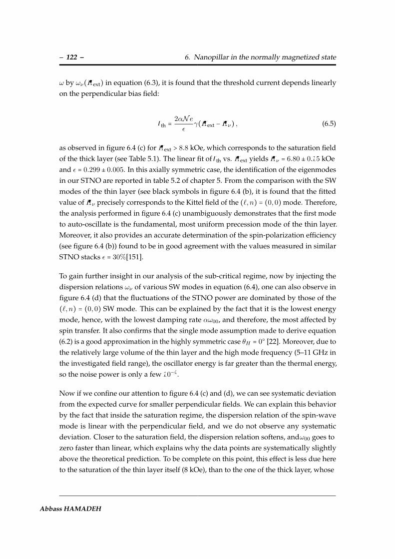
– 122 – 6. Nanopillar in the normally magnetized state
ω by ων(Hext) in equation (6.3), it is found that the threshold current depends linearlyon the perpendicular bias field:
Ith =2αN eε
γ(Hext −Hν) , (6.5)
as observed in figure 6.4 (c) for Hext > 8.8 kOe, which corresponds to the saturation fieldof the thick layer (see Table 5.1). The linear fit of Ith vs. Hext yields Hν = 6.80 ± 0.15 kOeand ε = 0.299± 0.005. In this axially symmetric case, the identification of the eigenmodesin our STNO are reported in table 5.2 of chapter 5. From the comparison with the SWmodes of the thin layer (see black symbols in figure 6.4 (b), it is found that the fittedvalue of Hν precisely corresponds to the Kittel field of the (`, n) = (0,0) mode. Therefore,the analysis performed in figure 6.4 (c) unambiguously demonstrates that the first modeto auto-oscillate is the fundamental, most uniform precession mode of the thin layer.Moreover, it also provides an accurate determination of the spin-polarization efficiency(see figure 6.4 (b)) found to be in good agreement with the values measured in similarSTNO stacks ε = 30%[151].
To gain further insight in our analysis of the sub-critical regime, now by injecting thedispersion relations ων of various SW modes in equation (6.4), one can also observe infigure 6.4 (d) that the fluctuations of the STNO power are dominated by those of the(`, n) = (0,0) SW mode. This can be explained by the fact that it is the lowest energymode, hence, with the lowest damping rate αω00, and therefore, the most affected byspin transfer. It also confirms that the single mode assumption made to derive equation(6.2) is a good approximation in the highly symmetric case θH = 0 [22]. Moreover, due tothe relatively large volume of the thin layer and the high mode frequency (5–11 GHz inthe investigated field range), the oscillator energy is far greater than the thermal energy,so the noise power is only a few 10−4.
Now if we confine our attention to figure 6.4 (c) and (d), we can see systematic deviationfrom the expected curve for smaller perpendicular fields. We can explain this behaviorby the fact that inside the saturation regime, the dispersion relation of the spin-wavemode is linear with the perpendicular field, and we do not observe any systematicdeviation. Closer to the saturation field, the dispersion relation softens, andω00 goes tozero faster than linear, which explains why the data points are systematically slightlyabove the theoretical prediction. To be complete on this point, this effect is less due hereto the saturation of the thin layer itself (8 kOe), than to the one of the thick layer, whose
Abbass HAMADEH
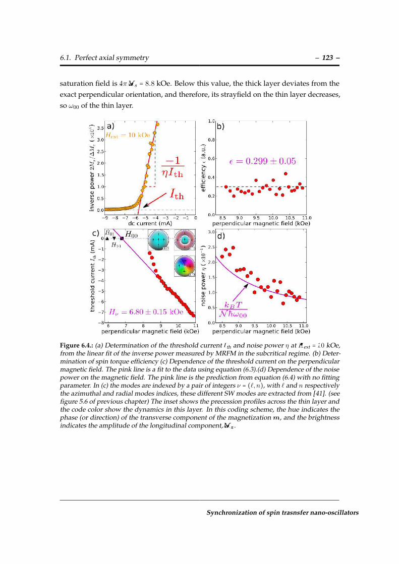
6.1. Perfect axial symmetry – 123 –
saturation field is 4πMs = 8.8 kOe. Below this value, the thick layer deviates from theexact perpendicular orientation, and therefore, its strayfield on the thin layer decreases,so ω00 of the thin layer.
Figure 6.4.: (a) Determination of the threshold current Ith and noise power η at Hext = 10 kOe,from the linear fit of the inverse power measured by MRFM in the subcritical regime. (b) Deter-mination of spin torque efficiency (c) Dependence of the threshold current on the perpendicularmagnetic field. The pink line is a fit to the data using equation (6.3).(d) Dependence of the noisepower on the magnetic field. The pink line is the prediction from equation (6.4) with no fittingparameter. In (c) the modes are indexed by a pair of integers ν = (`, n), with ` and n respectivelythe azimuthal and radial modes indices, these different SW modes are extracted from [41]. (seefigure 5.6 of previous chapter) The inset shows the precession profiles across the thin layer andthe code color show the dynamics in this layer. In this coding scheme, the hue indicates thephase (or direction) of the transverse component of the magnetization m, and the brightnessindicates the amplitude of the longitudinal component,Mz .
Synchronization of spin trasnsfer nano-oscillators

– 124 – 6. Nanopillar in the normally magnetized state
6.1.2. Forced regime
Now that the auto-oscillating SW mode has been identified, beside this, we discussits synchronization to an external signal [94, 90, 95, 96, 99]. Using the two differentmicrowave circuits, we shall compare the ability of the auto-oscillating mode to phase-lock either to the uniform microwave field hrf generated by the antenna or to themicrowave current irf flowing through the nanopillar. The dependence on Idc andHext of the SW modes excited by hrf (irf) is presented in figure 6.5a (6.5b). In theseexperiments, field-sweep MRFM spectra are acquired at fixed microwave frequency andIdc is decreased from 0 to −8.25 mA by steps of 50 µA. The color code shows the changein the longitudinal component ∆Mz produced by the amplitude modulation at fc of themicrowave source.
As aforementioned, in the exact perpendicular configuration, hrf selectively probes the` = 0 SW modes, whereas due to the orthoradial symmetry of the induced microwaveOersted field, irf couples to the ` = +1 SW modes [41]. The three main peaks of theMRFM spectra obtained at Idc = 0 in figures 6.5 (a) and 6.5 (b) are labeled according tothe SW mode identification see table 5.2 . B`n peaks correspond to SW modes dominatedby the thick PyB layer, while A00 and A10 are the fundamental harmonics of the thin PyAlayer with azimuthal indices ` = 0 and ` = +1, respectively. The resonant fields of thesetwo modes are similar, due to the different excitation frequencies used forhrf (8.1 GHz)and irf (9.2 GHz), i.e., A10 is 1.1 GHz higher in frequency than A00 [41].
Below the threshold current for the thin layer determined in Fig.6.4 c (indicated by themagenta lines in Fig.6.5), the observed behaviors of the ` = 0 and ` = +1 modes aresimilar: a small negative dc current slightly attenuates the thick layer SW modes B`n,while it promotes quite rapidly the SW modesA00 andA10 of the thin layer, in agreementwith STT [41]. On the contrary, there is a clear qualitative difference between the modesA00 and A10 beyond Ith. Although both peaks shift similarly towards lower field as ∣Idc∣is increased, A00 gets strongly distorted, with the appearance of a negative dip on itshigh field/large current side, in contrast to A10, which remains a positive peak.
A negative MRFM signal means that the precession angle in the thin layer is reduced inthe presence of the microwave excitation, see figure 6.6. This effect can be associated tothe synchronization of the auto-oscillating mode to the external signal [44], here hrf (andnot irf). In the so-called phase-locking range, its amplitude adapts ( ∆Mz > 0: increases,∆Mz < 0: decreases), so that the frequency of the auto-oscillation remains equal to the
Abbass HAMADEH

6.1. Perfect axial symmetry – 125 –
Figure 6.5.: (Color online). Dependence on Idc and Hext of the ` = 0 and ` = +1 SW modes,excited respectively by the uniform field hrf generated by the antenna at 8.1 GHz (a) and by theorthoradial Oersted field produced by the current irf flowing through the nanopillar at 9.2 GHz(b). The black traces are cuts of the MRFM signal vs. Idc at Hext = 0.88 T. The magenta obliquelines show the location of the threshold current determined in figure 6.4 (b). The black dashedlines are guides to the eye.
Synchronization of spin trasnsfer nano-oscillators
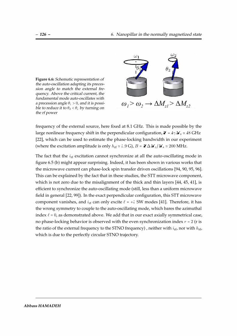
– 126 – 6. Nanopillar in the normally magnetized state
Figure 6.6: Schematic representation ofthe auto-oscillation adapting its preces-sion angle to match the external fre-quency. Above the critical current, thefundamental mode auto-oscillates witha precession angle θ1 > 0, and it is possi-ble to reduce it to θ2 < θ1 by turning onthe rf power
frequency of the external source, here fixed at 8.1 GHz. This is made possible by thelarge nonlinear frequency shift in the perpendicular configuration,N = 4γMs ≃ 48 GHz[22], which can be used to estimate the phase-locking bandwidth in our experiment(where the excitation amplitude is only hrf ≃ 1.9 G), B = N∆Mz/Ms ≃ 200 MHz.
The fact that the irf excitation cannot synchronize at all the auto-oscillating mode infigure 6.5 (b) might appear surprising. Indeed, it has been shown in various works thatthe microwave current can phase-lock spin transfer driven oscillations [94, 90, 95, 96].This can be explained by the fact that in these studies, the STT microwave component,which is not zero due to the misalignment of the thick and thin layers [44, 45, 41], isefficient to synchronize the auto-oscillating mode (still, less than a uniform microwavefield in general [22, 99]). In the exact perpendicular configuration, this STT microwavecomponent vanishes, and irf can only excite ` = +1 SW modes [41]. Therefore, it hasthe wrong symmetry to couple to the auto-oscillating mode, which bares the azimuthalindex ` = 0, as demonstrated above. We add that in our exact axially symmetrical case,no phase-locking behavior is observed with the even synchronization index r = 2 (r isthe ratio of the external frequency to the STNO frequency) , neither with irf, nor with hrf,which is due to the perfectly circular STNO trajectory.
Abbass HAMADEH

6.2. Broken axial symmetry – 127 –
6.2. Broken axial symmetry
We have shown in the previous sections the experimental data and their analysis in thehigh symmetry perpendicular configuration. We have identified the auto-oscillatingmode which is the lowest energy, most uniform SW mode of the thin layer. In additionwe have demonstrated that only a microwave magnetic field is efficient to synchronizethis auto-oscillating mode. Moreover we have seen that only ` = +1 modes are excited
by the RF current flowing through the nano-pillar, due to the orthoradial symmetry ofthe induced RF Oersted field produced by the rf current. Because there is no overlapbetween this particular excitation symmetry and the uniform azimuthal symmetry ofthe ` = 0 modes, the latter do not couple to the RF current excitation. Naletov et al. [41]demonstrated that the MRFM spectra excited by RF current change by introducing asmall angle θH between the applied field and the normal to the nano-pillar. In fact thischange is seen by the appearance of resonance peaks at the positions of ` = 0 modes. Itmeans that the latter can be excited by the rf current if the applied field is tilted awayfrom the normal to the nano-pillar. An open question in this case arises: what is theinfluence of the polar angle θH on the auto-oscillating mode? Is there some characteristicspectral features of this mode with the breaking of the axial symmetry?
In the following, we review the main experimental results that have been obtained whena small misalignment angle θH = 2 is introduced between the applied filed and thenormal to the layers. First, we experimentally report on the appearance of two modeswhen the sample is excited by a dc current flowing through the nano-pillar. Second, wehave cheeked what happens if one of these two modes is interacting with an externalsource. Here it contains both MRFM data and spectrum analyzer (SATM) (measurementof the voltage oscillations in the frequency domain) in order to report a comprehensiveanalysis of the data.
Synchronization of spin trasnsfer nano-oscillators

– 128 – 6. Nanopillar in the normally magnetized state
6.2.1. Autonomous regime
As already mentioned, stimulated emission favors the occurence of a single mode ofoscillation. Thus, only one mode is believed to auto-oscillate at the same time, thiscoincides with the basic assumption of the universal oscillator model, although jumpsbetween several auto-oscillating modes have been reported [152, 130, 131]. In thefollowing we shall show that mode competition can exist and there are situations wheretwo modes auto-oscillate at the same time in our STNO. In fact, as in a laser, a multimodeemission can occur, but this requires that the modes are phase decoupled. In our case,we will show that this condition is met for modes differring by their azimuthal index`.
Let us first focus on figure 6.7, which compares the MRFM spectra excited by a uniformRF magnetic field at 8.1 GHz to the one excited by an RF current flowing through thenano-pillar at same frequency. Theses spectra are acquired at different angle from theexact perpendicularity and at current Idc=0 (passive regime). Two important features areclearly visible, first, the ` = 0,1 SW modes spectrum are shifted towards lower field as θHincreases. Second, it is clear that the mode ` = 0 is excited by the RF current. These twoeffects have been explained in details in Reference [41]. To summarize, the resonancepeaks at θH = 2 are labeled according to the SW modes precession profiles and reportedin Table 6.1.
À Á Â Ã10.24 kOe 9.20 kOe 9.06 kOe 8.19 kOe
B00 B01 A00 A01
Ê Ë Ì Í10.24 kOe 9.77 kOe 8.72 kOe 8.62 kOe
B00 B10 B11 A10
Table 6.1.: The resonance fields values for the spin wave modes. The shown in blue (red) is thelocation of the SW modes measured experimentally in the figure 6.7 ( θH = 2) . Second line arethe experimental field peaks measured at f=8.1 GHz by sweeping the field.
Abbass HAMADEH

6.2. Broken axial symmetry – 129 –
Figure 6.7.: Eigen modes at θH = 2. Dependence of the mechanical-FMR spectra excited by auniform RF magnetic field (a) and by an RF current flowing through the nano-pillar (b) on thepolar angle θH between the applied field and the normal to the layers. Superposed (in violet) isthe behavior of the high field peak at larger power to reveal the effect better.
Synchronization of spin trasnsfer nano-oscillators

– 130 – 6. Nanopillar in the normally magnetized state
We have already mentioned that at θH = 2 it is possible to measure the auto-oscillationswith a SATM technique, this is due to the small change of relative angle between thickand thin layers while the latter is precessing.
Figure 6.8.: Power density spectrum as a function of cur-rent and applied magnetic field. Here a dc current isinjected to excite the thin layer via spin transfer. the twomode ` = 0 and ` = 1 have different critical current.
Now we will take advantage ofthis, and we will measure oursample by SATM technique. Werecall here that, we are able tomeasure this simultaneously tothe acquisition of the MRFM sig-nal. In figure 6.8, the evolutionof the auto-oscillation as a func-tion of the bias dc current Idc ispresented, the bias field beingfixed to Hext= 9.14 kOe. The po-sitions of the linear frequenciesof modes ` = 0 and ` = 1 at thisfield are determined by standardMRFM measurements in the lin-ear regime see table 6.1. f0 = 6.78+/- 0.12 GHz and f1= 7.95 +/- 0.2GHz are indicated by the hori-zontal blue and red rectangles, to-gether with the associated modeprofiles. Here, we drop the radial index n in the mode labeling (n = 0). From MRFMmeasurements, it is possible to follow the position of these two modes as a function ofIdc from the linear regime to the auto-oscillation regime, (same as shown before but withangle θH = 2 ) and to demonstrate that the two auto-oscillation peaks observed in figure6.8 between -6.5 and -8 mA indeed correspond to these two lowest energy modes ` = 0
and ` = 1 (see figure 6.11 in subsection 6.2.2).
Two main features can be noticed in the power spectrum of figure 6.8. The first one is thatthe threshold current for the two modes are different : the first peak, which correspond tothe mode ` = 0 visible until -6 mA. Starting from -6.5 mA the mode ` = 1 at GHz is visible.The second interesting feature is that beyond -8 mA, a simple one-mode generationregime is established in the system. At the moment, there is no clear understanding ofthe process leading to this transition. Here we will focus in the bi-modal region. For this,
Abbass HAMADEH

6.2. Broken axial symmetry – 131 –
it is important to note that we cannot tell anything about the relative powers p0 and p1
from the SA analyzer data, even if the modes do coexist. This is because for the sameexcitation amplitude of these two modes, a0 = a1, the voltage detection should yield alarger signal for the most uniform mode. Due to the mirror symmetry, there should notbe any high frequency voltage produced at f1 by the mode ` = 1. However, one shouldremember that due to the breaking of axial symmetry by the applied field, the ` = 1 modeprofile is actually slightly asymmetric (one precession lobe is larger than the other), andalso, that due to the Oersted field produced by the dc current flowing through the pillar,both the thick and thin Py layers should adopt a slightly curling configuration. Thiscould explain why a signal is actually detected. So to detect the total power generatedby the STNO, we use now the MRFM technique. Figure 6.9 displays the measurement ofthe STNO power vs. Idc, measured by MRFM for the same total bias field as in figure6.8 (taking into account the strayfield of the MRFM probe). For comparison, we haveplotted together with the data at θH = 2 those obtained at θH = 0. It is quite remarkablethat breaking the axial symmetry with the small tilt of the bias magnetic field leads tosuch a qualitative change. Here we measure all the power produced by the device. Theproblem is that we can’t separate the power generated by either mode (p = p0 + p1).But if we look to the range of the applied currents [-6 mA , -8 mA] we can see that thebehavior of the power change his slope, this is the signature of the presence of two modegeneration.
To make this more clear, we compare qualitatively the obtained measurements of thegenerated power in our nanopillar with a recent theoretical results [135]. RecentlySlobodianiuk [135] has presented a theory of microwave generation in STNOs in whichthe influence of increasing the thermal noise is taken into account. This theory showsthat an increase of thermal noise level is responsible of mediating a two-mode generationregime in STNO. The results of calculations performed using his model are presentedin figure 6.9 (a). Here the power are calculated numerically for a value of constantproportional to the temperature χ = 1.2 and the following parameters 4πγMs = 9500G,Γ0 = 60 MHz abd Γ1 = 1.05 Γ0. As we can see if we compare the experimentalmeasurements presented in figure 6.9 with the obtained theoretical results (figure 6.9), itis possible to describe the change of slope in the power generated by the STNO in therange of bias current (-6 and -8 mA) by starting the second mode. Indeed, as it’s clearfrom figure 6.9 by the addition of the two analytical expression obtained previously(red and blue curves) gives a qualitative estimate of the observed power generated bythe STNO. Then, we note here that this formalism description was done as a first step
Synchronization of spin trasnsfer nano-oscillators

– 132 – 6. Nanopillar in the normally magnetized state
(a) Mean powers calculated as a function of super-criticalities [135].
(b) Total power p emitted by the STNO as a func-tion of the bias dc current, measured by MRFM atθH = 0
and θH = 2.
Figure 6.9.: Qualitative Comparison between theoretical and experimental results
to determine the origin of the two mode observed experimentally in our device. Thecoupled equations are very important and very rich So we have only begun to explorethe behaviors of the power distribution in our STNO. Not doubt that future work willunravel with quantitive comparaison with the theory
Figure 6.10.: Frequency evolution of the free runningoscillations induced by spin transfer at Idc = −7 mA asa function of the magnetic field showing evidence thattwo modes auto-oscillate (` = 0,1).
To close this section on the au-tonomous dynamics of the bi-modalregime, we present in figure 6.10a more efficient way to distinguishthe features of current induced bi-modal excitations. This can be doneby keeping the current constant andsweeping the applied field instead.By doing we represent in figure 6.10the experiment obtained at constantbias current Idc = −7mA, by varyingthe bias magnetic field between 8.5and 9.6 kOe. This makes it possibleto tune the auto-oscillation frequen-cies f0 and f1 on a wider range thanwhat can be done at fixed field byvarying the current. In particular,
Abbass HAMADEH

6.2. Broken axial symmetry – 133 –
it is also worth to mention at this point that the fact that the frequency of the auto-oscillating modes strongly depends on the perpendicular field is an indication of non-linear damping. In fact, without a non-linear contribution to the damping, the generatedfrequency should remain constant (the larger the field, the smaller the precession angle,therefore the smaller the non-linear frequency shift).
6.2.2. Forced regime
The above experiments clearly show the presence of two modes. An open questionarises: are there interactions between them? is it possible to promote one of these twomodes by acting on the system with an external source and what happens?
First to investigate the non-autonomous dynamics in the previously identified bi-modalregime, we take advantage of our sample design, that allows us to add to the bias currentIdc either an in-plane homogenous RF field hrf or an RF current irf flowing through thelayers. So we use now the external source hrf and irf , while detecting the dynamics withMRFM. In figure 6.11 we have measured the spectral deformations produced on theSW spectra of figure 6.7 when a finite negative current is injected in the nanopillar, werecall that a negative dc current destabilizes the thin layer. Here the offset field fromthe MRFM magnetic probe has been subtracted and the amplitude of hrf is equal to1.9 Oe and irf is equal to 125 µA (which corresponds to an Oersted field of 2.8 Oe at theperiphery of the nano-pillar).
The main feature can be observed in the evolution of the SW spectra as Idc varied is anincrease of the modes associated to the thin layer. (we remember here that similar studyin the exact perpendicular geometry for −4 < Idc < 4 mA have been reported in reference[41]. The negative ∆Mz means that the precession angle is smaller when the RF is onthan when it is off, which is associated to lock-in to the external source. Based on thestudy discussed above (see figure 6.7) in the sub-critical regime, these two modes areidentified as the lowest energy spin-wave eigen-modes of the free layer with azimuthalnumbers `=0 and `=+1. The fact that these two modes ( =0 and `=+1) can auto-oscillateat the same time is made possible by the fact that each mode is living in his own spacedue to different spatial symmetry. The mutually exclusive nature of the responses tothe uniform and orthoradial symmetry excitations is a property of the preserved axialsymmetry, where the azimuthal index ` is here a good quantum number, i.e., different`-index modes are not mixed and can be excited separately.
Synchronization of spin trasnsfer nano-oscillators

– 134 – 6. Nanopillar in the normally magnetized state
Figure 6.11.: a) Evolution of the ` = 0 SW modes excited by a uniform RF magnetic field and b)of the ` = +1 SW modes excited by an RF current flowing through the nano-pillar as a functionof the negative dc current bias. The FMR spectra are acquired by MRFM at fixed frequencyf = 8.1 GHz by sweeping the applied magnetic field. The open (close) symbols indicate SWmodes associated to mainly the thin (thick) layer, and the dashed lines are guides to the eye.
To gain further insight about how above the threshold the two free-running modes areaffected by an external source. In figure 6.12, we present the experimental data obtainedin the same conditions as we present in figure 6.10 , plus with the external source hrf
at f=8.1 GHz (figure 6.12 (a)) and irf at f=9.2 GHz (figure 6.12 (b)). In both cases, oneobserves clearly that the auto-oscillating modes can be locked to an external sourcehaving the appropriate symmetry and a frequency close to the free-running frequencylight blue (light red) line in figure 6.12 (a) (figure 6.12 (b)). The striking result here isthat the external signal does not affect only the auto-oscillating mode which has its free-running frequency close to the external frequency and the appropriate spatial symmetry,but also the other auto-oscillating mode, in a quite similar way. It is particularly clearon figure 6.12 (a), where the external RF field synchronizes the ` = 0 auto-oscillatingmode between 9 kOe and 9.3 kOe at f=8.1 GHz: at the same time, the frequency ofthe ` = 1 mode becomes almost constant at slightly more than 9.2 GHz (see partiallytransparent light red line). Note that in contrast, hrf does not affect directly the ` = 1
mode at 8.1 GHz, around H=8.7 kOe, because it has the wrong spatial symmetry. Theinfluence of the RF current at f=9.2 GHz on the power density map of figure 6.12 (c) looksquite more complicated, but clearly, the behavior of mode ` = 0, whose free-running
Abbass HAMADEH

6.2. Broken axial symmetry – 135 –
Figure 6.12.: a) Behavior of the auto-oscillations at Idc = −7 mA in the free running oscillationand b) in the presence of the uniform RF field generated by the external antenna at 8.1 GHz(hrf = 2.7 G, thick blue line) and c) of the RF current flowing through the nano-pillar at 9.2 GHz(irf = 350 µA, thick red line).
frequency is about 1 GHz below the external source, is strongly affected on a broadrange of magnetic field. Here, when one tries to synchronize the ` = 1, the mode ` = 0
at f0 locks to an intermediate frequency between f0 and f1. To clarify this situation, itshould be remember that there is a asymmetric between rf field and rf current excitation.In particular, the rf current excitation excites the ` = 0 mode at θH = 2, while the inverseis not true: the rf magnetic field does not excite the ` = 1 mode at θH = 2. The differenceis explained above in the previous subsection. Thus when a rf current is injected insidethe ` = 0 mode will try to also synchronize with the f1 frequency. It thus shall move upin frequency by
√(f1 − f0)2 −∆2, where ∆ expresses on the strength of the ST-FMR.
The evolution of the ` = 0,1 modes as the power increases are also investigated. The spec-tral analysis of the mode ` = 1 is presented in figure 6.13a (frequency), 6.13b (linewidth)and 6.13c (amplitude). We can see how the pseudo-synchronization of the mode ` = 1
evolves: its range increases with power (same as the ` = 0 mode), but at the sametime, the pseudo-synchronization frequency also increases. A striking reduction of thelinewidth of the ` = 1 mode can also be observed, as it drops from almost 200 MHz downto less 50 MHz. A natural explanation would be some kind of mode cooling mecha-nism: by phase-locking the mode ` = 0 with the external source, its frequency, henceits amplitude, gets stabilized. As a result, its influence on the linewidth of mode ` = 1
through nonlinear cross-terms is suppressed. Hence, mode ` = 1 exhibits its intrinsiclinewidth, with the contribution of only self nonlinear interactions. See figure 6.14 for a
Synchronization of spin trasnsfer nano-oscillators

– 136 – 6. Nanopillar in the normally magnetized state
Figure 6.13.: a-c) Emission characteristics of the mode ` = +1 as a function of the amplitude of theuniform RF field used to lock the mode ` = 0 at 8.1 GHz (as in figure 6.12 (a)): center frequency,linewidth, and amplitude, from top to bottom. e-f) Emission characteristics of the mode` = 0 asa function of the amplitude of the RF current used to lock the mode` = +1 at 9.2 GHz (as in 6.12(b) )
Abbass HAMADEH

6.2. Broken axial symmetry – 137 –
direct experimental evidence of this mode cooling in the frequency domain.
As already stated before, the behavior of auto-oscillations in the bi-modal regime inthe presence of the external source irf looks more complex. But looking at the powerdependence in figure 6.13 (d) to (f) does help a little bit to understand what is going on. Infact, it is clear that the frequency of the mode` = 0 would like to jump to some constantfrequency branch somewhere around 8.5 GHz, in between the two auto-oscillatingmodes. At low power, it does not do it in one step, but reather in two, as it is clearfrom figure 6.13 (d). It is difficult to comment on the variation of the linewidth and ofthe amplitude, which are plotted in figure 6.13 (e) and (f), as the previously mentionedsteps introduce some broadening, and also, there are some weak broad features at lowerfrequency than the main peak. At the same time, it is hard to see what is happening withmode ` = 1. It looks like it almost disappears from the power map, still there is someweak broad feature above the external frequency f=9.2 GHz. Finally, we recall here thatthe SA measurements do not permit to follow the auto-oscillations in the close vicinity ofthe external frequency, because the latter is adding a huge signal to the STNO’s emission,which is hidden under the thick blue and red continuous lines in figure (6.12).
Figure 6.14: Mode cooling introduced in thediscussion of figure 6.13. We remind thestriking result here: the linewidth of themode ` = 1 that auto-oscillates at 9.2 GHzdecreases by more than a factor 4 (here, from183 to 39 MHz) when the ` = 0 mode, whichauto-oscillates at a frequency 1.1 GHz be-low the mode ` = 1, gets phase-locked to theexternal uniform RF field. The upward fre-quency shift (100 MHz) which accompaniesthis mode cooling is also clearly recorded.
Synchronization of spin trasnsfer nano-oscillators

– 138 – 6. Nanopillar in the normally magnetized state
6.2.3. Synchronization: SATM data vs. MRFM data
Figure 6.15.: a) Magnetic field dependence of the STNOfrequency in the free and forced regimes (the externalsource at 8.1 GHz is h rf). b) Comparison between theSTNO frequency shift deduced from (a) and the MRFMsignal.
We have already mentioned thatour experimental setup allows tomonitor the ac voltage producedacross the nano-pillar by the pre-cession of the magnetization inthe bi-layer structure. A spec-trum analyzer is used to measurethe ac voltage across the nano-pillar when the Idc current passthrough the sample. This can bedone simultaneously to the acqui-sition of the MRFM signal, in theexact same conditions. Taking ad-vantage of this, one can comparethe auto-oscillation frequency inthe free (black squares in figure6.15 (a)) and forced regimes (bluedots). The resulting frequencyshift (blue dots in 6.15 (b)) canthen be quantitatively comparedto the MRFM signal, that has acharacteristic shape with a pos-itive and negative lobes aroundthe center frequency (black line, which is a cut at constant cur-rent Idc = −7mA of figure 6.11(a)). From this, we can also again confirm that in the so-called phase-locking range, theSTNO amplitude adapts (∆Mz > 0: increases, ∆Mz < 0: decreases), so as to maintainits frequency equal to the frequency of the source, here fixed at 8.1 GHz (see figure6.6). This comparison also allows to estimate the phase-locking bandwidth, found to beas large as 0.2 GHz despite the small amplitude of the external signal. From this, onecan determine the nonlinear frequency shift N = ∆Mz/(MsB) ≃ 85 GHz. This value ismuch larger than N = 4γMs. In fact the nonlinear frequency shift N strongly dependson the angle of the applied field. Its largest value is reached in the exact perpendicular
Abbass HAMADEH
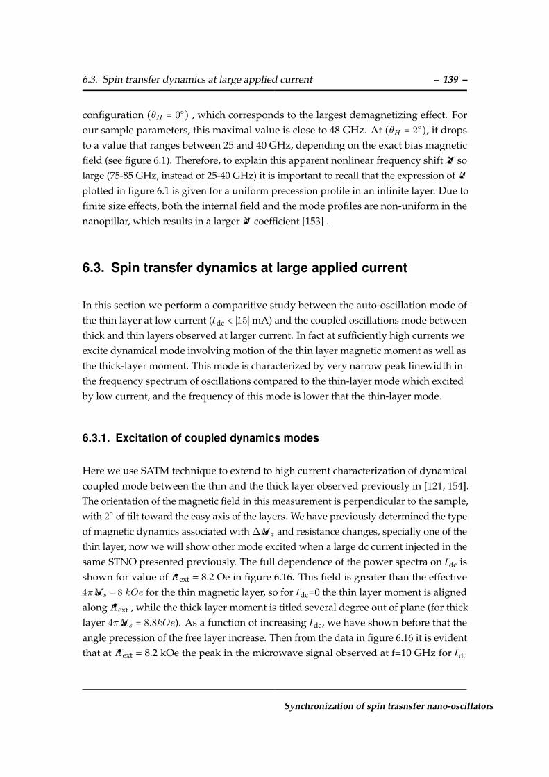
6.3. Spin transfer dynamics at large applied current – 139 –
configuration (θH = 0) , which corresponds to the largest demagnetizing effect. Forour sample parameters, this maximal value is close to 48 GHz. At (θH = 2), it dropsto a value that ranges between 25 and 40 GHz, depending on the exact bias magneticfield (see figure 6.1). Therefore, to explain this apparent nonlinear frequency shift N solarge (75-85 GHz, instead of 25-40 GHz) it is important to recall that the expression of Nplotted in figure 6.1 is given for a uniform precession profile in an infinite layer. Due tofinite size effects, both the internal field and the mode profiles are non-uniform in thenanopillar, which results in a larger N coefficient [153] .
6.3. Spin transfer dynamics at large applied current
In this section we perform a comparitive study between the auto-oscillation mode ofthe thin layer at low current (Idc < ∣15∣ mA) and the coupled oscillations mode betweenthick and thin layers observed at larger current. In fact at sufficiently high currents weexcite dynamical mode involving motion of the thin layer magnetic moment as well asthe thick-layer moment. This mode is characterized by very narrow peak linewidth inthe frequency spectrum of oscillations compared to the thin-layer mode which excitedby low current, and the frequency of this mode is lower that the thin-layer mode.
6.3.1. Excitation of coupled dynamics modes
Here we use SATM technique to extend to high current characterization of dynamicalcoupled mode between the thin and the thick layer observed previously in [121, 154].The orientation of the magnetic field in this measurement is perpendicular to the sample,with 2 of tilt toward the easy axis of the layers. We have previously determined the typeof magnetic dynamics associated with ∆Mz and resistance changes, specially one of thethin layer, now we will show other mode excited when a large dc current injected in thesame STNO presented previously. The full dependence of the power spectra on Idc isshown for value of Hext = 8.2 Oe in figure 6.16. This field is greater than the effective4πMs = 8 kOe for the thin magnetic layer, so for Idc=0 the thin layer moment is alignedalong Hext , while the thick layer moment is titled several degree out of plane (for thicklayer 4πMs = 8.8kOe). As a function of increasing Idc, we have shown before that theangle precession of the free layer increase. Then from the data in figure 6.16 it is evidentthat at Hext = 8.2 kOe the peak in the microwave signal observed at f=10 GHz for Idc
Synchronization of spin trasnsfer nano-oscillators

– 140 – 6. Nanopillar in the normally magnetized state
Figure 6.16.: Microwave power density as a function of frequency and current, measured for anexternal magnetic field Hext = 8.2 Oe. The frequency of the mode of the thin layer grows linearlyas a function of current. At Idc=-20mA the mode drops from free layer mode to a coupling modebetween the thin and the thick layer.
as small as -8 mA, correspond to small angle precession of the thin layer (this modeis labeled as A© ). After as function of increasing Idc up to -8 mA, the frequency of themicrowave signal increases. This behavior was observed previously in figure 6.8 and itwas identified with the increasing of ∆Mz i.e power. Here the maximum frequency atwhich our amplifier is working is 18 GHz, this is why the microwave signal is shownin this range of frequency (4 - 18 GHz). For larger Idc, at approximately -25 mA, themicrowave signal exhibits a dramatic drop to a frequency 6 GHz with a simultaneousjump in power density (mode labeled as B©). This step can be explained by a reversalof the free layer’s precession axis to anti-parallel to the thick layer. Indeed, the largenegative currents apply a torque on the thin and thick layers which are strongly coupledby their spin transfer torques as well as by dipolar coupling between the layers. Thenthe resulting is a coupling mode between the thin and the thick layers, which correspondto a precession of the thick layer, likely coupled to the thin layer.
6.3.2. Characterization of coupled dynamics modes
Our main objective is to compare the output rf signal characteristics for the cases ofa dynamics free layer mode and a dynamics coupled thin and thick mode. For this
Abbass HAMADEH
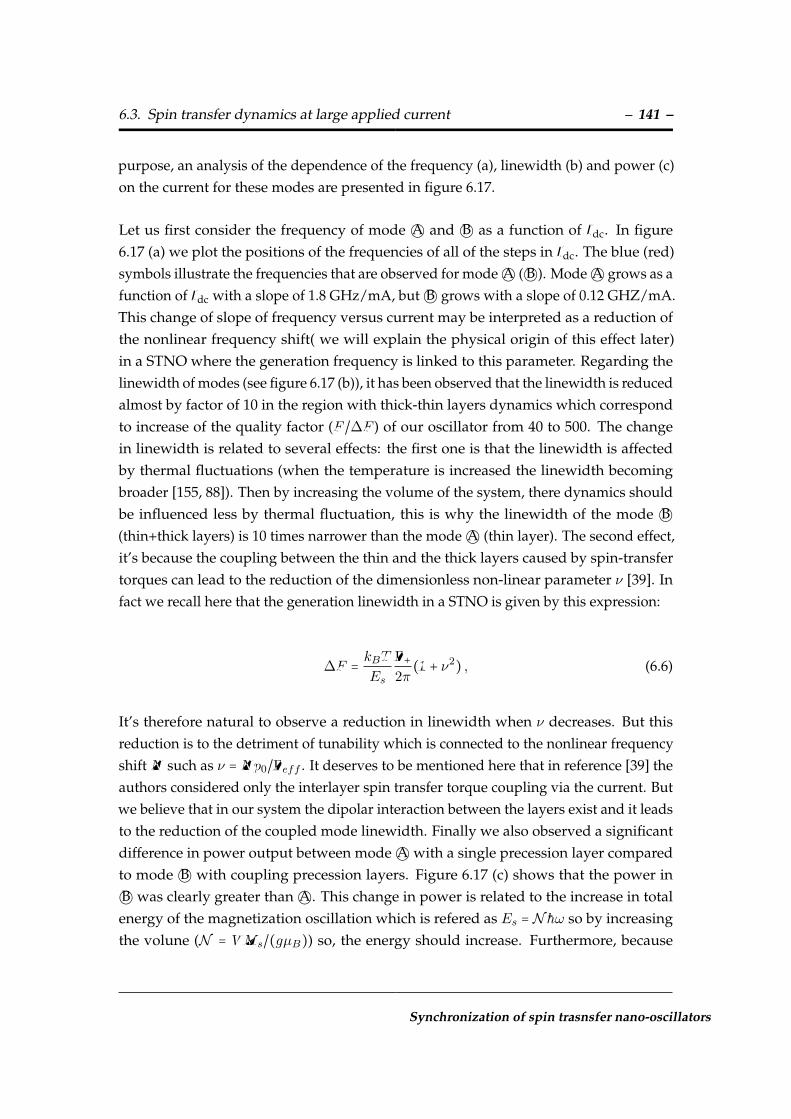
6.3. Spin transfer dynamics at large applied current – 141 –
purpose, an analysis of the dependence of the frequency (a), linewidth (b) and power (c)on the current for these modes are presented in figure 6.17.
Let us first consider the frequency of mode A© and B© as a function of Idc. In figure6.17 (a) we plot the positions of the frequencies of all of the steps in Idc. The blue (red)symbols illustrate the frequencies that are observed for mode A© ( B©). Mode A© grows as afunction of Idc with a slope of 1.8 GHz/mA, but B© grows with a slope of 0.12 GHZ/mA.This change of slope of frequency versus current may be interpreted as a reduction ofthe nonlinear frequency shift( we will explain the physical origin of this effect later)in a STNO where the generation frequency is linked to this parameter. Regarding thelinewidth of modes (see figure 6.17 (b)), it has been observed that the linewidth is reducedalmost by factor of 10 in the region with thick-thin layers dynamics which correspondto increase of the quality factor (F /∆F ) of our oscillator from 40 to 500. The changein linewidth is related to several effects: the first one is that the linewidth is affectedby thermal fluctuations (when the temperature is increased the linewidth becomingbroader [155, 88]). Then by increasing the volume of the system, there dynamics shouldbe influenced less by thermal fluctuation, this is why the linewidth of the mode B©(thin+thick layers) is 10 times narrower than the mode A© (thin layer). The second effect,it’s because the coupling between the thin and the thick layers caused by spin-transfertorques can lead to the reduction of the dimensionless non-linear parameter ν [39]. Infact we recall here that the generation linewidth in a STNO is given by this expression:
∆F = kBTEs
Γ+2π
(1 + ν2) , (6.6)
It’s therefore natural to observe a reduction in linewidth when ν decreases. But thisreduction is to the detriment of tunability which is connected to the nonlinear frequencyshift N such as ν = Np0/Γeff . It deserves to be mentioned here that in reference [39] theauthors considered only the interlayer spin transfer torque coupling via the current. Butwe believe that in our system the dipolar interaction between the layers exist and it leadsto the reduction of the coupled mode linewidth. Finally we also observed a significantdifference in power output between mode A© with a single precession layer comparedto mode B© with coupling precession layers. Figure 6.17 (c) shows that the power inB© was clearly greater than A©. This change in power is related to the increase in totalenergy of the magnetization oscillation which is refered as Es = N hω so by increasingthe volune (N = VMs/(gµB)) so, the energy should increase. Furthermore, because
Synchronization of spin trasnsfer nano-oscillators

– 142 – 6. Nanopillar in the normally magnetized state
Figure 6.17.: Spectral analysis on the full range of bias dc current. The blue color is used tohighlight the auto-oscillating mode of the thin layer, while the red color highlights the collectivemode between thin and thick layers.
Abbass HAMADEH

6.4. Conclusion – 143 –
these oscillations occur at large current values, they can produce larger microwave signalthan the thin layer oscillations.
6.4. Conclusion
The nature of the auto-oscillating mode in a spin transfer nano-oscillator based onnormally magnetized nano-pillar has been investigated using the MRFM and SATMtechnique. In particular, we considered the high symmetric case between the appliedfield and the axis of the nano-pillar, as this configuration coincides with the quanti-tative model proposed by Slavin et al. [22], as well as asymmetric cases by tilting theapplied field 2 from the sample normal. Our results show that:
i) The auto-oscillating mode in high symmetric case consists of the lowest energymode (((` = 0,n = 0))) dominated by the thin layer.
ii) Only a spatially homogenous microwave magnetic field is efficient to synchro-nize this auto-oscillating mode.
iii) Two modes can be excited in the asymetric case (((` = 0,n = 0))) and (((` = 1,n = 0))) .
iv) Evidence of a non-linear coupling between these two modes which are auto-oscillating at the same time has been experimentally demonstrated.
v) The coupled mode involving both the thin and thick layers excited at large cur-rent has improved microwave characteristics (linewidth, power) compared to thesingle mode dominated by the thin layer. We ascribe this mainly to a decreaseof non-linearities, as evidenced by the reduction of tunability in the case of cou-pled mode.
Synchronization of spin trasnsfer nano-oscillators


CHAPTER 7
Nano-pillar in the double-vortex state
This chapter is dedicated to the study of a spin valve nano-pillar structure with coupledmagnetic vortices. The sample investigated in the previous chapter is reconsidered,thus, now with nucleation of two vortices, one in each ferromagnetic layer. Indeed, theSTNO presented previously can also sustain gyrotropic vortex motion, with generatedfrequencies below 2 GHz, and is capable of operating under zero applied magnetic field.After, the microwave signal emitted by the STNO will be measured by SATM techniquein order to investigate the non-linear characteristics of this device in the vortex state.Moreover, the influence of an external source on the microwave signal generated by thisSTNO will be highlighted.
145

– 146 – 7. Nano-pillar in the double-vortex state
7.1. Introduction
We have already presented the spin transfer nano-oscillators based on the excitationof the quasi uniform precession mode. In these experiments high external magneticfields were required to observe microwave output signals. In 2007 Pribiag et al. havedemonstrated that spin torque can also drive a magnetic vortex into gyration [33].The microwave frequency oscillations of magnetic vortex have been observed bothin nano-pillar [33, 35] and nano-contact geometry [156, 79]. Recently it has also beendemonstrated that such vortex based STNO might work in absence of external field [85].Therefore, these results allow considering the magnetic vortex motion as an importantconfiguration of the spin torque nano-oscillator. Then, it became very interesting tostudy the vortex configuration not only from fundamental point of view but also asa promising class of new generation of nano-scale functional microwave devices . Inparticular, very narrow linewidths [40] and large TMR output signal [35] are promisingfor the applications. In this section, we will introduce the particular case of STNO basedon coupled magnetic vortices [40].
Dynamics of two coupled vortices in STNO
As mentioned previously, the integration of STNOs in high frequency circuits dependson various conditions. The important parameters are the linewidth, and the generatedpower signal. Further research efforts are being devoted to optimization of these parame-ters. Recently, to increase the power of the signal of the STNO based vortex, a new devicewas proposed by A. Dussaux et al.[35]. The device is circular shape nanopillar with aradius of 85 nm patterned from the whole magnetic stack : synthetic anti-ferromagnetMgO (1.075 nm)/NiFe (15 nm)/capping. In this configuration, the vortex dynamics isconverted into a microwave signal thanks to the large magneto-resistive ratio of theTunnel Magnetoresistance effect (TMR) leading to microwave emissions combininglarge power (5 nW). But the linewidth in this device is limited to 1 MHz. In order, toimprove the spectral linewidth of the vortex oscillator. One solution proposed in ametallic system is to use a spin transfer nano-oscillator driven dynamics of coupledvortices. Indeed, recently Locatelli et al.[40] demonstrated that two coupled vortices ina metallic nanopillar can reduce the linewidth of the microwave signals, see figure 7.1(c). It has been also shown that, using injected current and external magnetic field, itis possible to independently control and discriminate vortex chiralities and polarities
Abbass HAMADEH
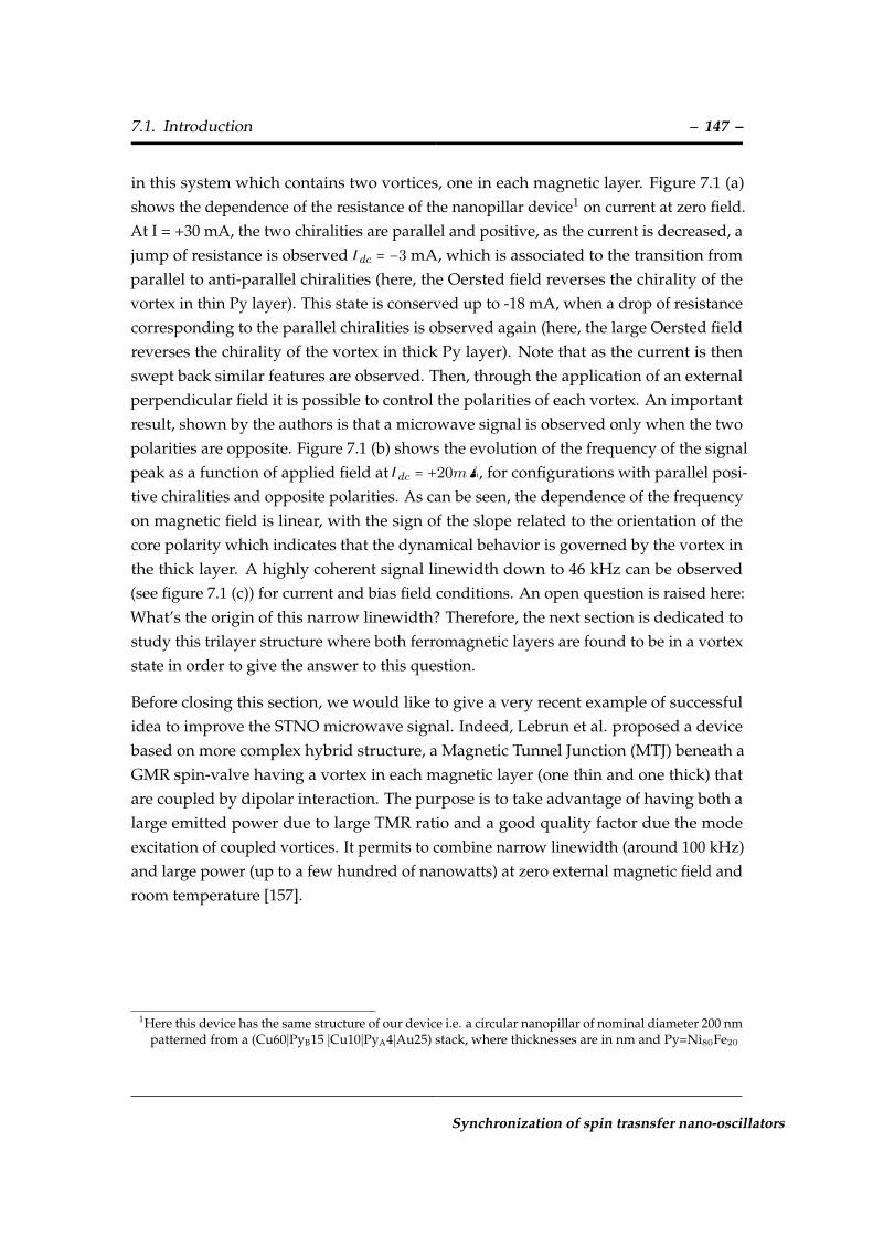
7.1. Introduction – 147 –
in this system which contains two vortices, one in each magnetic layer. Figure 7.1 (a)shows the dependence of the resistance of the nanopillar device1 on current at zero field.At I = +30 mA, the two chiralities are parallel and positive, as the current is decreased, ajump of resistance is observed Idc = −3 mA, which is associated to the transition fromparallel to anti-parallel chiralities (here, the Oersted field reverses the chirality of thevortex in thin Py layer). This state is conserved up to -18 mA, when a drop of resistancecorresponding to the parallel chiralities is observed again (here, the large Oersted fieldreverses the chirality of the vortex in thick Py layer). Note that as the current is thenswept back similar features are observed. Then, through the application of an externalperpendicular field it is possible to control the polarities of each vortex. An importantresult, shown by the authors is that a microwave signal is observed only when the twopolarities are opposite. Figure 7.1 (b) shows the evolution of the frequency of the signalpeak as a function of applied field at Idc = +20mA, for configurations with parallel posi-tive chiralities and opposite polarities. As can be seen, the dependence of the frequencyon magnetic field is linear, with the sign of the slope related to the orientation of thecore polarity which indicates that the dynamical behavior is governed by the vortex inthe thick layer. A highly coherent signal linewidth down to 46 kHz can be observed(see figure 7.1 (c)) for current and bias field conditions. An open question is raised here:What’s the origin of this narrow linewidth? Therefore, the next section is dedicated tostudy this trilayer structure where both ferromagnetic layers are found to be in a vortexstate in order to give the answer to this question.
Before closing this section, we would like to give a very recent example of successfulidea to improve the STNO microwave signal. Indeed, Lebrun et al. proposed a devicebased on more complex hybrid structure, a Magnetic Tunnel Junction (MTJ) beneath aGMR spin-valve having a vortex in each magnetic layer (one thin and one thick) thatare coupled by dipolar interaction. The purpose is to take advantage of having both alarge emitted power due to large TMR ratio and a good quality factor due the modeexcitation of coupled vortices. It permits to combine narrow linewidth (around 100 kHz)and large power (up to a few hundred of nanowatts) at zero external magnetic field androom temperature [157].
1Here this device has the same structure of our device i.e. a circular nanopillar of nominal diameter 200 nmpatterned from a (Cu60∣PyB15 ∣Cu10∣PyA4∣Au25) stack, where thicknesses are in nm and Py=Ni80Fe20
Synchronization of spin trasnsfer nano-oscillators

– 148 – 7. Nano-pillar in the double-vortex state
Figure 7.1.: Resistance evolution versus dc-current, measured at zero external magnetic field.Schematics represent the magnetic configuration in thin Py(4nm) and thick Py(15nm) layers, bigarrows correspond to vortices chiralities. Low resistance is associated to the observation of two-vortices state with identical chiralities, whereas hight resistance is associated to the observation oftwo-vortices state with opposite chiralities. Here, the increase of resistance associated with Jouleheating was subtracted. (b) Dependence of microwave frequencies on perpendicular magneticfield for I=20 mA and configurations with positive chiralities and opposite polarities. The redcircles show experimental data obtained for p1 = +1 and p2 = 1. The blue triangles show thesymmetric case. (c) Microwave peak with ∆F = 46 kHz for H = 66 mT and I = 20 mA. Thecontinuous red line is a Lorentzian fit to the data. Figures taken from reference [40]
7.2. Autonomous regime: analysis of linewidth and tunability
A particularity of STNOs compared to other oscillators is their strong nonlinear prop-erties, which are inherited from the equation of motion of magnetization [22]. On onehand, they confer interesting properties to STNOs, as for instance their large frequencytunability [120, 158]. On the other hand, they lead to a severe broadening of the gen-eration linewidth [23]: due to nonlinear phase-amplitude coupling, the phase noise ofSTNOs is indeed rather large [24, 25], which is the main limiting factor to their practicalapplications.
As we mentioned previously, some of the best microwave characteristics have beenreported for STNOs in which spin transfer torque (STT) excites the gyrotropic mode ofa magnetic vortex [33]. It results in microwave emission in the range 100 MHz −2 GHzcharacterized by a narrow linewidth (about 1 MHz) and large output power in the caseof TMR devices [35]. Moreover, the oscillation frequency of vortex-based STNOs can berapidly modified between different values using the bias current, which demonstratestheir high agility and tunability in current [159]. Recently, Locatelli et al. have reporteda record high spectral purity (quality factor Q > 15000) in a spin-valve nano-pillar where
Abbass HAMADEH

7.2. Autonomous regime: analysis of linewidth and tunability – 149 –
STT drives the dynamics of two coupled vortices (one in each ferromagnetic layer)[40]. In such a STNO, the generation linewidth at fixed dc current Idc displays strongvariations (from 40 kHz to 1 MHz) on the applied perpendicular field H⊥. At the sametime, its frequency tunability dF /dIdc ≃ 7 MHz/mA remains almost constant whichpoints out that spectral purity and tuning sensitivity are not necessarily correlated. Inthis section, we aim at understanding the physical origin of these peculiar behaviors, asthis will give hints to optimize the characteristics of STNOs.
7.2.1. High frequency properties
Figure 7.2.: Upper right sketch: STNO based on coupled vortices. (a) Power density spectrameasured at Idc = 20 mA and a perpendicular magnetic field H⊥ = −0.7 kOe and (b) H⊥ =−0.15 kOe. (c) Dependence of the fundamental oscillation frequency on H⊥.
Here, the studied STNO is the same sample investigated in the previous chapter, but,now with the non-uniform magnetization profile of both layers i.e two vortices, one ineach ferromagnetic layer. Indeed, our STNO can sustain the double vortex configuration
Synchronization of spin trasnsfer nano-oscillators

– 150 – 7. Nano-pillar in the double-vortex state
[40, 160]. We remember that a current Idc > 0 is injected through the STNO using thebottom Cu and top Au electrodes, which corresponds to electrons flowing from the thickPyB to the thin PyA layer. In both Py layers, the vortex chiralities are parallel to theorthoradial Oersted field produced by Idc. We use a magnetic field H⊥ perpendicular tothe sample plane in order to control the relative orientation of the vortex core polaritiespAand pB. As shown in Ref.[40], we observe a narrow microwave signal only in the
case when they are opposite, pApB = −1, and when Idc exceeds a threshold currentIth ≃ 8 to 11 mA depending on H⊥. The spontaneous microwave emission branch atIdc = 20 mA for which pA = +1 and pB = −1 is displayed in figure 7.2 (c). The oscillationfrequency linearly decreases with increasing H⊥, as expected for a gyrotropic modedominated by the thick layer vortex, whose polarity is antiparallel to the applied field[61]. The observed emission frequency, which decreases from 750 MHz to 450 MHzas H⊥ increases from −0.7 kOe to 3 kOe, agrees well [40] with the expected gyrotropicfrequency for the thick PyB layer augmented with the contributions of the Oersted field[76, 83] and of the dipolar coupling to the thin PyA layer [161]. The boundaries of thefrequency branch shown in figure 7.2 (c) result from the combined action of H⊥ and STTto reverse the vortex cores in the Py layers [162].
7.2.2. Origin of narrow linewidth
Our aim is to understand why the linewidth of our oscillator can increase by morethan a factor 20 (up to 1 MHz), and moreover what is the necessary condition to obtainthe highest spectral purity. For this purpose, let’s first concentrate on the dependenceof the generation linewidth on H⊥, which is plotted in figure 7.3 (a) using dark bluesymbols (∆F1). It displays minima down to 40 kHz (F1/∆F1 ≃ 19000) and maxima upto 1 MHz (F1/∆F1 ≃ 700), i.e., a decrease of spectral purity by more than a factor 25 bychanging H⊥ from −0.7 kOe [figure 7.2 (a)] to −0.15 kOe [figure 7.2 (b)]. We first note thatthe strong variations of the linewidth observed at Idc = 20 mA cannot be attributed tochanges of the nearly constant supercriticality (Idc/Ith ≃ 2) or integrated power (0.32 pWat H⊥ = −0.7 kOe vs. 0.4 pW at H⊥ = −0.15 kOe (see figures .7.2 (a) and (b)). As alreadymentioned, the generation linewidth of a nonlinear auto-oscillator can be written as[23]:
∆Fg =kBT
Es
Γ+2π
(1 + ν2) , (7.1)
Abbass HAMADEH

7.2. Autonomous regime: analysis of linewidth and tunability – 151 –
Figure 7.3.: (a) Generation linewidths of harmonics n = 1 to 4 divided by n2 as a function of H⊥.(b) Frequency tunability vs. H⊥. Inset: dependence of the oscillation frequency on Idc measuredat H⊥ = 0 kOe.
we recall here that, kB is the Boltzmann constant, T the temperature, Es the energy storedin the auto-oscillation, Γ+ the natural energy dissipation rate, and ν the nonlinear phase-amplitude coupling parameter. The latter is defined as ν = Np/Γp, the dimensionlessratio between the nonlinear frequency shift N multiplied by the normalized oscillationpower p and divided by the damping rate of amplitude fluctuations Γp [22].
Since the spectral linewidth ∆Fg depends quadratically on ν, the dependence of this pa-rameter on H⊥ should be evaluated. For this, we analyze the linewidth of the harmonicsof the auto-oscillation signal. It was shown in Reference [163] that the linewidth ∆Fn ofthe nth harmonics is related to the fundamental one (∆F1) by:
1
n2= ∆F1 (
1 + ν2
∆Fn− ν2 1 − exp (−2Γp/∆Fn)
2Γp) . (7.2)
Synchronization of spin trasnsfer nano-oscillators

– 152 – 7. Nano-pillar in the double-vortex state
We have plotted in figure 7.3 (a) the evolution of ∆Fn/n2 (n = 2 to 4) together withthe one of ∆F1. It is clear from this graph that independently of H⊥, ∆Fn ≃ n2∆F1,which means that our STNO is quasi-isochronous and from equation (7.2), that ν ≃ 0
in the full field range. Therefore, one can also exclude that the strong variations oflinewidth observed in figure 7.3 (a) are due to some changes of ν with H⊥. Moreover, wecan estimate the generation linewidth from equation (7.4) when ν = 0. For the vortexgyrotropic mode with angular frequency ω, Es = 1
2GωX2, where G = 2πLMs/γ is the
gyrovector and X the gyration radius of the core and Γ+ = ηαω [77]. For the thick PyB
layer (L = 15 nm), Ms = 764 emu.cm−3, γ = 1.87 ⋅ 107 rad.s−1.Oe−1 and the dampingcoefficient α = 0.008 were determined by mechanical ferromagnetic resonance [41],and the topological renormalization of damping is η = 1.7 [76]. From micromagneticsimulations [164], the radius of gyration under bias conditions close to the experimentalones is found to be X ≃ 40 nm (corresponding to p = (X/R)2 ≃ 0.1). Hence, at roomtemperature, kBT /Es ≃ 0.003 and Γ+/(2π) = 9.5 MHz, which yields ∆Fg = 29 kHz, avalue close to the narrow linewidth of 40 kHz observed at Hext = −0.7 kOe [figure 7.2(a)], which thus almost coincides with the intrinsic linewidth of our oscillator. In sum,the absence of nonlinear broadening and the large energy stored in the auto-oscillationin comparison to the thermal energy explain the low minimal values (< 100 kHz) of thelinewidth in figure 7.3a.
7.2.3. Origin of tunability
Before seeking further the origin of the variations of linewidth, we first investigatepossible physical causes of quasi-isochronicity. Despite the fact that the nonlinearity ν ofour STNO is nearly zero, it exhibits a large frequency tunability,dF /dIdc ≃ 7 MHz/mA,see figure 7.3 (b). This can be explained by the linear contribution of the Oersted field tothe oscillation frequency. In fact, the tunability can be decomposed as follows:
dF
dIdc= ∂F∂p
∂p
∂Idc+ ∂F
∂Idc= N ∂p
∂Idc+AOeIdc . (7.3)
In the vortex state, the Oersted field participates to the confinement potential of thevortex core [76, 83], and for our STNO parameters, it is predicted to be about AOe ≃12.5 MHz/mA. Therefore, a nonlinear frequency shift N ≠ 0 is not required to obtain alarge tuning sensitivity in equation (7.3). Here, the measured tunability is comparablewith the one expected for the Oersted field alone. We attribute the somewhat smallerexperimental value to the fact that the auto-oscillating mode does not only involve the
Abbass HAMADEH
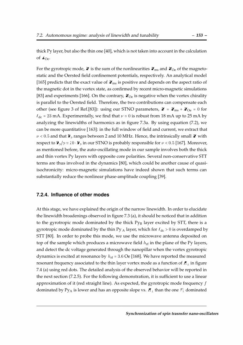
7.2. Autonomous regime: analysis of linewidth and tunability – 153 –
thick Py layer, but also the thin one [40], which is not taken into account in the calculationof AOe.
For the gyrotropic mode, N is the sum of the nonlinearities Nms and NOe of the magneto-static and the Oersted field confinement potentials, respectively. An analytical model[165] predicts that the exact value of Nms is positive and depends on the aspect ratio ofthe magnetic dot in the vortex state, as confirmed by recent micro-magnetic simulations[83] and experiments [166]. On the contrary, NOe is negative when the vortex chiralityis parallel to the Oersted field. Therefore, the two contributions can compensate eachother (see figure 3 of Ref.[83]): using our STNO parameters, N = Nms + NOe = 0 forIdc = 23 mA. Experimentally, we find that ν ≃ 0 is robust from 18 mA up to 25 mA byanalyzing the linewidths of harmonics as in figure 7.3a. By using equation (7.2), wecan be more quantitative [163]: in the full window of field and current, we extract thatν < 0.5 and that Γp ranges between 2 and 10 MHz. Hence, the intrinsically small N withrespect to Γp/p ≃ 10 ⋅ Γp in our STNO is probably responsible for ν < 0.5 [167]. Moreover,as mentioned before, the auto-oscillating mode in our sample involves both the thickand thin vortex Py layers with opposite core polarities. Several non-conservative STTterms are thus involved in the dynamics [80], which could be another cause of quasi-isochronicity: micro-magnetic simulations have indeed shown that such terms cansubstantially reduce the nonlinear phase-amplitude coupling [39].
7.2.4. Influence of other modes
At this stage, we have explained the origin of the narrow linewidth. In order to elucidatethe linewidth broadenings observed in figure 7.3 (a), it should be noticed that in additionto the gyrotropic mode dominated by the thick PyB layer excited by STT, there is agyrotropic mode dominated by the thin Py A layer, which for Idc > 0 is overdamped bySTT [80]. In order to probe this mode, we use the microwave antenna deposited ontop of the sample which produces a microwave field hrf in the plane of the Py layers,and detect the dc voltage generated through the nanopillar when the vortex gyrotropicdynamics is excited at resonance by hrf = 3.6 Oe [168]. We have reported the measuredresonant frequency associated to the thin layer vortex mode as a function of H⊥ in figure7.4 (a) using red dots. The detailed analysis of the observed behavior will be reported inthe next section (7.2.5). For the following demonstration, it is sufficient to use a linearapproximation of it (red straight line). As expected, the gyrotropic mode frequency fdominated by PyA is lower and has an opposite slope vs. H⊥ than the one F1 dominated
Synchronization of spin trasnsfer nano-oscillators

– 154 – 7. Nano-pillar in the double-vortex state
Figure 7.4.: (a) Blue dots: fundamental frequency F1 and harmonics F2 of the auto-oscillatingmode dominated by the thick layer (vortex core polarity pB = −1) as a function of H⊥. Red dots:frequency f of the overdamped mode dominated by the thin layer (polarity pA = +1). Red tonestraight lines are guides to the eye and show successive harmonics of f . (b) Evolution of theinverse generation linewidth. (c) Slope of the oscillation frequency F1 vs. H⊥.
by PyB, due to smaller thickness (LA < LB) and opposite core polarity (pA = +1 = −pB)[61]. We also note that the linewidth of this mode ranges between 80 and 100 MHz,which is about 8 times larger than its natural linewidth, in agreement with the increase
Abbass HAMADEH

7.2. Autonomous regime: analysis of linewidth and tunability – 155 –
of relaxation of the thin layer due to STT.
Using red tone lines in figure 7.4 (a), we have plotted its harmonics n = 2 to 5 togetherwith the measured fundamental frequency F1 and harmonics F2 of the auto-oscillationsignal (blue dots). We have also reported in figures 7.4 (b) and (c) the inverse generationlinewidth (logarithmic scale) and the slope −dF1/dH⊥ of the oscillation frequency vs.H⊥, respectively. At magnetic fields where the frequencies of the auto-oscillating andoverdamped modes are commensurable, pF1 = qf , with p, q ∈ N (dashed vertical linesin figure 7.4 (a)), a decrease of −dF1/dH⊥ concomitant with a decrease of the inverselinewidth is observed. We attribute this behavior to the interaction between the eigen-modes of the STNO. When they cross each other, their frequency dispersions soften [100]and some energy can be transferred from the auto-oscillating mode to the overdampedmode. As a result, this additional channel of relaxation leads to a decrease of the coher-ence time of the auto-oscillation (this effect is not taken into account in equation (7.4),which was derived in a single mode approximation [22]). Here, the dynamic dipolarinteraction [169, 170] is an obvious source of coupling between modes, but we stressthat the dissipative STT terms at play in the double vortex configuration can also beimportant [80]. More theoretical work would be required to describe the multi-modeautonomous dynamics of our STNO [130]. Still, the main finding reported in figure 7.4can be expressed in general terms, valid for all STNOs: the ratio of energy stored toenergy lost in the system decreases when the auto-oscillating mode becomes degeneratewith the overdamped mode. Since the coupling strength depends on the difference inenergy between the modes, we emphasize that the STNO should better be operatedunder conditions where large frequency gaps exist between the auto-oscillating modeand other modes in the system [88, 111, 112].
7.2.5. Self parametric excitation
Parametric excitations of magnetization oscillations have been largely considered in thefield of ferromagnetic resonance [171, 172]. These interesting phenomena are excitedwhen the cycle of modulation of the oscillation is repeated twice during one period T0 ofnatural oscillations in the elementary system, i.e., when the frequency Ω of parametricmodulation is twice the natural frequency Ω0 of the system. The first observation ofparametric excitation of an STNO is given by Urazhdin et al.[173]. The authors havedemonstrated that a microwave magnetic field, applied at frequency equal to twicethe resonance frequency of the nano-contact STNO where the magnetic free layer is
Synchronization of spin trasnsfer nano-oscillators

– 156 – 7. Nano-pillar in the double-vortex state
uniformly magnetized leads to parametric resonance. Recently, Bortolotti et al.[174],have demonstrated that a microwave current flowing through a vortex-based MTJ STNOprovided enough Oersted field to parametrically excite the vortex gyration. In addition,the same phenomena have been investigated in the case of a uniformly magnetizedfree layer at room-temperature where parametric excitation can also be obtained of thenon-vortex high-frequency modes in MTJ STNOs by using a microwave current [175].
In this section, based on our experimental observations, we suggest the concept ofself-parametric excitation in a STNO having one vortex in each magnetic layer. It is acase of self-parametric because the field used to modulate the frequency of magnetizationoscillations isn’t generated by an external source. It is instead produced by the auto-oscillation of the vortex in the thick layer. Indeed, when the frequency of the vortex inthe thick layer comes close to twice the frequency of the lowest frequency mode presentin the thin layer with vortex ground state, parametric excitation of this damped layercan be achieved. These studies are aimed for understanding the physical source of thepeculiar behaviors on the frequency of the thin layer observed in figure 7.4 (a) in theprevious subsection.
7.2.5.1. Spectral measurement
First, the dependence of the frequencies of the 2 gyrotropic modes on the externalmagnetic field of the microwave signal emitted by the STNO are reported again in figure7.5. We recall here that there are two gyrotropic modes in our system, the first one isdominated by the thick PyB layer (blue) which is excited by STT (this dynamical mode ischaracterized by measurement of auto-oscillation induced at bias current I > Ith in theabsence of the external driving signal). The second mode is dominated by the thin PyA
layer (red), which for Idc > 0 is overdamped by STT. In order to excite this mode, we haveused microwave antenna deposited on top of the sample which produces a microwavefield hrf in the plane of the thin layer, and we have detected the dc voltage generatedthrough the nanopillar when the vortex gyrotropic dynamics is excited at resonance byhrf = 3.6 Oe [168].
The main features of the voltage spectra are modified when the frequency f of the thinlayer is close to the half of the frequency of the thick layer i.e. f=F/2. In the insets offigure 7.5, we present the voltage signal as a function of the frequency of the externalmicrowave signal source. As shown in inset [i] the spectrum measured at H⊥ = −50 Oe
Abbass HAMADEH

7.2. Autonomous regime: analysis of linewidth and tunability – 157 –
Figure 7.5: (a) Blue dots: funda-mental frequency F of the auto-oscillating mode dominated by thethick layer (vortex core polaritypB = −1) as a function of H⊥. Reddots: frequency f of the over-damped mode dominated by thethin layer (polarity pA = +1). Reddots lines are guides to the eye andshow 2*f. Insets: Spectroscopic de-tection at Idc = +20 mA of the thinlayer vortex spectrum excited by auniform RF magnetic field. (b) Evo-lution of the generation linewidthof the thin layer.
can be fitted by a Lorentzian distribution. The corresponding linewidth of this spectrumis 80 MHz, which is about 8 times larger than the natural linewidth, in agreement withthe increase of relaxation of the thin layer due to STT. In fact in the vortex state, thedamping multiplier η = (1/2) ln (R/(2LE)) + 5/8, where LE = 6 nm is the exchangelength in Py, equals η = 1.7 for both Py layers [76]. For simplification, we neglect thecoupling between the thin and thick Py layers, i.e., we assume that the overdampedand auto-oscillating modes only involve the thin and thick layers, respectively. In thatcase, Γ+,A/(2π) = ηαAωA/(2π) = 7.1 MHz and Γ+,B/(2π) = ηαBωB/(2π) = 9.6 MHz atHperp = 0 kOe. Below the threshold current Ith, the linewidth is given by [22]:
∆ω = 2Γ+ (1 − Idc
Ith) . (7.4)
The threshold current for the mode dominated by the thin layer is about Ith,A = −3 mA.Therefore, at Idc = 20 mA, the linewidth of the overdamped mode is predicted to be∆f = 2 ⋅ Γ+,A/(2π) ⋅ (1 + 20/3) ≃ 108 MHz, in good agreement with the measured value(80 − 100 MHz).
Synchronization of spin trasnsfer nano-oscillators

– 158 – 7. Nano-pillar in the double-vortex state
The shape of the spectrum changes drastically in a large window of H⊥ between 0.1 and1.5 kOe. A striking example of such feature is displayed in the second inset [ii] for aperpendicular magnetic field equal to H⊥ = 0.3kOe. We find that the voltage spectrumis completely changed in this range, in which the signal associated with the vortexexcitation becomes negative and positive and the spectral linewidth reduces significantlyfrom 80 to 10 MHz. In this range, the vortex frequency decreases linearly with H⊥ and isstrictly equal to F/2. For H⊥ outside this range, the voltage spectra is again Lorentzianshape with linewidth 80 MHz. To show the drastic improvement of the linewidth ofthe signal, we plot in figure 7.5 (b) the linewidth of the peak detected as a function ofperpendicular magnetic field. As we can see, when f is equal to F/2, the linewidth of thesignal decreases. The minimum fitted linewidth reaches 11 MHz. These measurementsare consistent with the effect observed on the linewidth the ones presented by Urazhdinet al. [173] for the case of uniform magnetization under a parametric rf field. Furtherproof of self-parametric excitation is provided by the observation of microwave signalin the SA at a frequency close to F/2 . In figure 7.6 , we present two typical spectrameasured for H⊥ = 1.3 and H⊥ = 1.8 kOe. Indeed, a signal appears from the backgroundlevel only when 0.1 < H⊥ < 1.5 kOe , which corresponds to a frequency about twicethe natural frequency F of the vortex oscillation in the thick layer. It is not possible toobserve a parametrically excited signal for a magnetic field out of this range.
In order, to explain this observation of the self-parametric excitation STNO, we haveestimated analytically the average dynamical dipolar field induced by the vortex gyra-tion of the thick layer on the thin layer in the case of our STNO geometry. We find thatthe amplitude of the dipolar field for a radius of gyration under bias conditions close toX ≃ 40 nm is about 200 Oe, which is sufficiently large to excite parametrically the vortexin the thin layer. In fact, at resonance, a large dipolar field must be generated on the thinlayer by the thick layer to make the vortex in the thin move periodically ‘oscillate’ atfrequency F/2 [174].
As a final comment, in contrast to previous studies 2 presented by Urazhdin et al. , wefound a significant increase from 11 MHz to 30 MHz of the linewidth close to the pointwhen f should be equal exactly F/2. We speculate that the reason here for this featureis the same that described previously in section 7.2.4, where we have shown that thelinewidth of a STNO increases at the crossing of modes.
2Here the authors shows that minimum linewidth is observed near to zero detuning i.e, when the frequencyof the STNO is equal to the frequency of the external source divided by two
Abbass HAMADEH

7.2. Autonomous regime: analysis of linewidth and tunability – 159 –
Figure 7.6: (a) Self-parametric exi-tation of the vortex in the thin layerat Idc = 20 mA measured by the SA.The measured spectra for H⊥ =1.3kOe shows 2 peaks one at F = 610MHz and another at F/2 which cor-responds to the excitation of thethin layer. The inset shows a zoom.(b) Measured spectra for Idc = 20mA and H⊥=1.8 kOe . Only onepics at F=575 MHz is observed.
7.2.5.2. Threshold and bandwidth of self-parametric excitation
Parametric resonance is possible only when a threshold is exceeded, that is, when theincrement of energy during a period caused by the parametric variation is larger thanthe amount of energy spread out during the same time. To meet this requirement, thedepth of modulation must past some critical value. This threshold value of the depthof modulation depends on the damping in the material [171, 173, 174]. Nevertheless, ifthe threshold is exceeded, the frictional losses of energy cannot restrict the growth ofthe amplitude. Moreover, one of the most interesting features of parametric resonanceis the possibility of exciting oscillations not only at exactly 2F, but also in intervalsof frequencies lying on either side of the values 2F (in the range of instability). Thisbandwidth becomes wider as the range of parametric variation is extended, that is, asthe amplitude of modulation is increased. Usually in parametric excitation studies thedriving amplitude is controlled by the external source, while in our experiment wecan tune the amplitude via the DC current injected in the device. When we increase(decrease) the current the amplitude of the oscillation increases (decreases), as a result
Synchronization of spin trasnsfer nano-oscillators

– 160 – 7. Nano-pillar in the double-vortex state
Figure 7.7.: Frequency boundaries of the self-parametric excitation region vs Idc.
the dipolar field increase (decrease). The dependence of the self-parametrically inducedoscillation spectra on the current is summarized in figure 7.7. The blue and red squaresin this plot mark the boundaries of the instability region for the given pumping current,which are defined by the condition that the oscillation frequency of the thin layers isequal to F/2. The width of the instability region increases with the increase of the current,and vanishes when Idc approaches the threshold value Ith determined by the dynamicmagnetic damping in the Py disk and the amplitude of oscillation of the vortex in thethick layer. Our data demonstrate that self-parametric excitation cannot be achievedin the thin layer at Idc= 9 mA without oscillation of the vortex in the thick layer. Thefrequency range of the self-parametrically excited oscillations increases approximatelylinearly with increasing Idc, confirming that this variation is dominated by the amplitudeof the dipolar field generated by the thick layer which grows linearly with the current[83].
Abbass HAMADEH

7.3. Forced regime – 161 –
7.3. Forced regime
Synchronization to an external periodic signal and mutual phase-locking of severalSTNOs have been suggested as a way to increase the emitted power and reduce the phasenoise of STNOs. It has been successfully demonstrated that phase locking of an arrays ofJosephson junctions 3 leads to increase the power as a squares of the numbers of junctions[93], and it is a general assumption that the ocillating coherently of N oscillators, reducethe phase noise by a factor of aboutN [176]. It has also been proposed that synchronizedarrays of STNOs could be operated as associative memories [177]. So far, mutual phase-locking has been achieved using spin wave coupling between nanocontacts [27, 28, 30]and 2D arrays of vortices and anti-vortices [29]. It is also predicted to occur usingthe common microwave current emitted [97, 26] or the dipolar interaction betweenadjacent STNOs [178, 179]. To demonstrate the efficiency of these two types of coupling,synchronization to an external microwave current passing through the device [94, 90,96, 95] or to a microwave field produced by an external antenna [99, 158] have beenstudied.
Two key characteristics to analyze the quality of the synchronization are the lockingrange and the generation linewidth in the phase-locked regime, which are respectivelyrelated to the coupling efficiency and the response to noise of the oscillator. In a singlevortex-based tunneling magnetoresistance (TMR) device, it was shown that using anexternal microwave current, the locking range could reach up to one third of the oscillatorfrequency, and the linewidth be reduced by 3 orders of magnitude, from a few MHzdown to 3 kHz [95].
We have discussed the microwave signal generated by the dynamics of two coupledvortices in a spin-valve oscillators in detail. In this section, we investigate the casewhen such a system is subjected to a external microwave source. For this purpose,the microwave emissions are recorded on the spectrum analyzer and injection lockingexperiments are performed by adding a microwave field from an external source. Thecharacteristics of the signal will be measured in the phase-locked regime and we willshow experimentally and analytically the influence of the linewidth on the couplingbetween the signal emitted by the STNO and an external microwave signal.
3The josephson junction is a system very close to the STNO
Synchronization of spin trasnsfer nano-oscillators

– 162 – 7. Nano-pillar in the double-vortex state
7.3.1. Synchronization at fundamental frequency
We have shown that above a current of about +10 mA, a narrow microwave emissionpeak is observed on the spectrum analyzer, which corresponds to the spin transfer drivendynamics of the two coupled vortices. At fixed Idc, the microwave characteristics of thisauto-oscillation peak (frequency and linewidth) can be tuned by varying H⊥. In thisstudy, all measurements were carried out at room temperature. The dc current injectedthrough the nanopillar was fixed to Idc = 15 mA or varied by ±4% around this valuewhen specified. The maximal output power from the synthetizer (source frequency Fs)injected into the microwave antenna was +10 dBm, corresponding to hrf = 6.3 Oe.
Figure 7.8.: Power spectrum map of the STNO atIdc = 15 mA and H0 = 1 kOe vs. the frequency Fs ofthe external microwave field hrf = 2 Oe.
In the first experiment, the perpendic-ular field is set to H⊥ = 1 kOe. Underthese bias conditions, the oscillatorfrequency is F0 = 586 MHz and thegeneration linewidth ∆F0 = 142 kHz.In figure 7.8, we present a map of thepower density recorded on the spec-trum analyzer when the frequencyFs of the external microwave field isswept from 540 MHz to 630 MHz andthe driving field amplitude is set tohrf = 2 Oe. When Fs comes closer toF0, the frequency of the oscillator ispulled towards the source frequency.When Fs ≃ 574 MHz, there is a sin-gle frequency peak in the spectrum,meaning that the auto-oscillation issynchronized to the external source.At this point, it is not possible to sep-arate the signal of the gyrotropic auto-oscillation and that of the source, which preventsmeasuring the generation linewidth in the phase-locked regime. This situation is ob-served until Fs ≃ 597 MHz, above which the auto-oscillation frequency comes back to itsfree running value F0.
Figure 7.9.: Locking range ∆ as a function of the driveamplitude.
The locking range ∆ measuredexperimentally is plotted vs. the
Abbass HAMADEH

7.3. Forced regime – 163 –
driving field amplitudehrf in fig-ure 7.9. As expected [22], it in-creases linearly with hrf at lowdriving amplitude (hrf < 1.5 Oe).The behavior observed at largerhrf is presumably due to somenonlinearities of the system. Wepoint out that at hrf = 6.3 Oe,the locking range ∆ = 75 MHzcorresponds to 13% of the oscil-lator frequency F0. Moreover,we emphasize that there is nosynchronization to the externalmicrowave current irf passingthrough the STNO based on cou-pled vortices, in contrast to thesituation presented in figure 7.8, where the microwave field hrf is very efficient to phase-lock the signal. A similar behavior was observed in the saturated state of the samedevice and ascribed to symmetry reasons [158].
7.3.2. Fractional synchronization
Since the peaks observed at F when the oscillator is synchronized at the fundamentalfrequency F are dominated by the parasitic coupling to the driving external source signal.We have performed a second measurement in which the microwave signal generated bythe oscillator is locked to the source when its frequency Fs is equal to some fractions ofF0. Figure 7.10 shows the PSD map of the output voltage for the STNO frequency F0
versus the driving frequency Fs. It is clear that the frequency F0 of the driven STNOfollows the driving frequency Fs not only in the vicinity of the point Fs = F0 but also thelocking is observed near to the points Fs=3F0/2,Fs=2F0 and Fs=3F0. We note here thatthese fractional synchronization are not related to the source nonlinearity, because wehave checked that no subharmonics were emitted by the source, in particular, at 1/3Fs,1/2Fs and 2/3Fs. Moreover, the power emitted in the second and third harmonic of thesource is 40 dB smaller than the power emitted at the main frequency.
Synchronization of spin trasnsfer nano-oscillators

– 164 – 7. Nano-pillar in the double-vortex state
Figure 7.10.: Power spectrum map of the STNO at Idc = 15 mA and H0 = 1 kOe vs. the frequencyFs of the external microwave field hrf = 6.3 Oe. The source frequency Fs is swept from 200 MHzto 1850 MHz, the insets are zoom for the synchronization showing 3/2 Fs, 2Fs and 3 Fs.
7.3.3. Perfect and robust synchronization
In order to caracterize quatitativly the linewidth of the oscillator signal when its fre-quency is locked, an example when the source frequency Fs is swept around 2F0 is showin figure 7.11 (a). Here, we plot the frequency shift Fforced −F0 of the oscillator when it isforced by the microwave field of amplitude hrf = 6.3 Oe as a function of Fs varying from1150 MHz to 1190 MHz. As in figure 7.11 (a), we observe the characteristic behaviorof synchronization to the external source, except that it is now at twice the oscillatorfrequency and the oscillation signal is not hindered by the source signal. Hence, we cananalyze the dependence of the generation linewidth on Fs, which is plotted in figure 7.11(b). The striking observation is a dramatic reduction of the generation linewidth withinthe locking range. As shown in the inset of figure 7.11 (b), the measured linewidth is in-deed limited by the 1 Hz minimal RBW of the spectrum analyzer, i.e., the auto-oscillationis perfectly phase-locked to the external source. This corresponds to an improvement ofthe signal coherency by a factor greater than 105 with respect to the free running case.The increase of the generation linewidth up to 1 MHz observed at the boundaries ofthe locking range is attributed to successive synchronization-unsynchronization eventsoccurring at the timescale of the measurement [95].
To gain further insight, we investigate the robustness of this perfect phase-locking.
Abbass HAMADEH
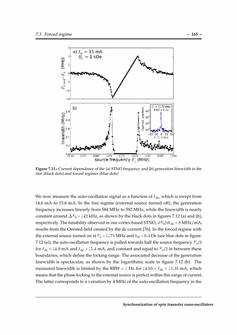
7.3. Forced regime – 165 –
Figure 7.11.: Current dependence of the (a) STNO frequency and (b) generation linewidth in thefree (black dots) and forced regimes (blue dots)
We now measure the auto-oscillation signal as a function of Idc, which is swept from14.6 mA to 15.6 mA. In the free regime (external source turned off), the generationfrequency increases linearly from 584 MHz to 592 MHz, while the linewidth is nearlyconstant around ∆F0 = 142 kHz, as shown by the black dots in figures 7.12 (a) and (b),respectively. The tunability observed in our vortex-based STNO, dF0/dIdc ≃ 8 MHz/mA,results from the Oersted field created by the dc current [76]. In the forced regime withthe external source turned on atFs = 1175 MHz and hrf = 6.3 Oe (see blue dots in figure7.12 (a)), the auto-oscillation frequency is pulled towards half the source frequency Fs/2for Idc < 14.9 mA and Idc > 15.4 mA, and constant and equal to Fs/2 in between theseboundaries, which define the locking range. The associated decrease of the generationlinewidth is spectacular, as shown by the logarithmic scale in figure 7.12 (b). Themeasured linewidth is limited by the RBW = 1 Hz for 14.93 < Idc < 15.35 mA, whichmeans that the phase-locking to the external source is perfect within this range of current.The latter corresponds to a variation by 4 MHz of the auto-oscillation frequency in the
Synchronization of spin trasnsfer nano-oscillators

– 166 – 7. Nano-pillar in the double-vortex state
free regime. These features demonstrate the robustness of the synchronization observedin our sample, as it means that even if the external source frequency deviates fromthe oscillator frequency by more than ten times the free running linewidth, perfectphase-locking can still occur.
Figure 7.12.: Current dependence of the (a) STNO frequency and (b) generation linewidth in thefree (black dots) and forced regimes (blue dots).
Abbass HAMADEH
7.3. Forced regime – 167 –
7.3.4. Role of noise in phase-locking phenomena
Another issue to investigate is the influence of fluctuations on the actual characteristics ofour vortex oscillator when it is phase-locked. To do that, we compare the synchronizationof auto-oscillation signals having different generation linewidths. We use two differentapplied fields, H0
⊥= +1 kOe and H1
⊥= −0.27 kOe, at which the emission frequencies
at Idc = 15 mA slightly differ (F0 = 586 MHz and F1 = 684 MHz, respectively), andthe generation linewidth varies by more than a factor seven, from ∆F0 = 142 kHz to∆F1 = 1.05 MHz (see inset of figure .7.13 (a)). Using blue and red dots at H0
⊥and H1
⊥,
respectively, we plot the experimental frequency mismatch Fforced − Fs/2 (figure .7.13(a)) and the linewidth in the forced regime (figure .7.13 (b)) as a function of the detuningF0,1 − Fs/2 between the natural oscillator frequency and half the source frequency. Thestrong differences observed in the characteristics of the synchronization at these twofields reveal the role played by the fluctuations in the phase dynamics of STNOs. Whenthe latter are weak (narrower generation linewidth at H0
⊥), the locking range is large
(more than 4 MHz) and the synchronized signal acquires the spectral quality of thesource (less than 1 Hz). When the noise is larger (broader generation linewidth at H1
⊥), it
competes against the coupling to the external source, which results in a smaller apparentlocking range and a poorest spectral quality of the forced oscillation. Here, increasingthe linewidth by a factor ∆F1/∆F0 ≃ 7 has a huge influence on the signal coherency inthe phase-locked regime since its improvement with respect to the free running casedrops from a factor 105 to only 10.
In order to model these experimental results, we employed the theory from reference[90, 91]. According to this model, the mismatch Fforced − Fs/2. of a noisy oscillator isrelated to the detuning frequency ∆FDet = F0 − Fs/2. via the locking strength ε in thefollowing expression:
Fforced − Fs = −∆FDet − εIm
⎡⎢⎢⎢⎢⎢⎢⎣
1
2 i∆FDet−w2
ε + 1
2i∆FDet−2w2
ε+...
⎤⎥⎥⎥⎥⎥⎥⎦
. (7.5)
Where w2 is the noise of the oscillator, expressed as its natural linewidth. Now Onecan use equation 7.5 and compare it to the experimental observation.The influence ofphase fluctuations on the frequency mismatch has been shown by continuous lines infigure .7.13 (a). Using the measured linewidths ∆F0 and ∆F1 in the equation 7.5, the
Synchronization of spin trasnsfer nano-oscillators

– 168 – 7. Nano-pillar in the double-vortex state
only fitting parameter is the coupling strength of the external microwave source to theoscillator (equal to half the locking range in the case of zero fluctuations), which is foundto be ε = 2.5 MHz both at H0 and H1.
Figure 7.13.: (a) Variation of the frequency mismatchFforced − Fs/2 as a function of the detuningF0,1 − Fs/2 at H0
⊥= +1 kOe (blue dots) and H1
⊥= −0.27 kOe (red dots). The external source
amplitude is set to hrf = 6.3 Oe. Continuous lines are fits using Eq.(5) of Ref.[90] yielding acoupling strength ε = 2.5 MHz. The inset shows the emission spectra at H0
⊥and H1
⊥in the free
running regime. (b) Dependence of the emission linewidth on the frequency detuning at H0⊥
andH1⊥
.
Abbass HAMADEH
7.4. Conclusion – 169 –
7.4. Conclusion
In this chapter, we have investigated the microwave characteristics of a spin transfernano-oscillator based on coupled vortices as a function of the perpendicular mag-netic field H⊥. By analyzing the harmonic content of the spectrum, we find that ourSTNO is quasi-isochronous independently of H⊥, which suppresses the severe non-linear broadening usually observed in STNOs. Still the generation linewidth dis-plays strong variations onH⊥ (from 40 kHz to 1 MHz), while the frequency tunabilityin current remains almost constant (7 MHz/mA). This demonstrates that isochronic-ity does not necessarily imply a loss of frequency tunability, which is here governedby the current induced Oersted field. It is not sufficient either to achieve the high-est spectral purity in the full range of magnetic field. We show that the observedlinewidth broadenings are due to the excited mode interacting with a lower energyoverdamped mode, which occurs at the successive crossings between harmonics ofthese two modes.
We have also reported that the strong dynamic dipolar field induced by the spin trans-fer driven excitation of the mode dominated by the thick layer is able to parametri-cally excite the damped mode dominated by the thin layer. The excitation bandwidthincreases with the dc current, which is consistent with our interpretation. These re-sults are important not only to understand the behavior of the freqeuncy of the thinlayer in our system, but also for the synchronization of STNO arrays.
In addition, we have also studied the synchronization of this spin transfer drivenvortex dynamics to an external source. Phase-locking to the microwave field hrf oc-curs in a range larger than 10% of the oscillator frequency for drive amplitudes ofonly a few Oersteds. Using fractional synchronization at the double frequency, weanalyzed the behavior of the generation linewidth. It is found to decrease by morethan 5 orders of magnitude in the phase-locked regime (down to 1 Hz, limited by theresolution bandwidth of the spectrum analyzer) in comparison to the free runningregime (140 kHz). We find that the phase-locking remains perfect for frequency de-tunings as large as 2 MHz, which proves its robustness. We also analyzed how thephase noise in the free running regime influences the characteristics of the synchro-nization.
Synchronization of spin trasnsfer nano-oscillators
– 170 – 7. Nano-pillar in the double-vortex state
Abbass HAMADEH
CHAPTER 8
Dipolar coupling between adjacent STNOs
We have studied in detail the synchronization of a STNO to an external microwavesource. Here we extend these ideas to more interesting situations when two STNO areinteracting through dynamic dipolar coupling. In this chapter, we study the behaviorof the coupled vortex based STNOs. We start with giving the device structure andcharacterization. Then we illustrate some features of synchronization of these STNOspair and briefly discuss synchronization properties.
171

– 172 – 8. Dipolar coupling between adjacent STNOs
8.1. Introduction to mutual synchronization
We have already demonstrated that in the saturated state, there is a very efficient cou-pling of the auto-oscillations to an RF field (external antenna), and no coupling to the RFcurrent flowing through the device. We have also verified experimentally in the previouschapter that the same synchronization rules apply to the double vortex STNO structure.Therefore, we have identified a coupling mechanism to obtain mutual synchronizationbetween N STNOs, namely, the dipolar field. Indeed, to date, three different possi-ble coupling mechanisms between STNOs have been proposed: spin wave coupling,electrical coupling and dipolar coupling . In the electrical coupling design, the STNOsare electrically connected in series or parallel. Thus, the mechanism to couple severalcomes from the common microwave current emitted by and shared through the devices[26]. In this mechanism, the STNOs have to be connected to the same electrical circuit, sothe constraint on the separation between individual devices in the network isn’t required.The requirement to achieve self-synchronization is only on the amplitude of the emittedmicrowave current, which depends on the magnetoresistance ratio and on the type ofmagnetization dynamics that is excited. So far, there has been no experimental proof ofself-synchronization using this global coupling, but individual STNOs have successfullybeen phase-locked to an external source [94, 95, 90, 96]. There are others designs thatare based on local couplings which arise from exchange and dipolar energies, and aremediated by spin waves and dipolar fields between closest neighbors in an array ofSTNOs. Due to the exponential attenuation of propagating spin waves with distance dand 1/d3 decay of dipolar fields, these two types of coupling are effective below a typicallength scale of 1 µm, which is much larger than the separation that can be defined bylithography between adjacent STNOs ( ∼50 nm). Mutual synchronization of STNOshas been achieved for the first time using two adjacent nano-contacts patterned on acommon ferromagnetic layer, acting as a medium for propagating spin waves [28, 27].Pairwise synchronization by the spin wave mechanism in devices with four nano con-tacts has also been demonstrated [30]. A theoretical work combining micro-magneticsimulations and analytical calculations performed by demonstrated that this dipolarinteraction is also very efficient to synchronize several STNOs in the vortex state [ 178].Regarding mutual synchronization of vortex state auto-oscillations we have decided toperform a first experimental study [80] of dipolar coupling using only a pair of STNOsplaced nearby laterally. This study has been carried out in collaboration with the groupCNRS/Thales (Nicolas Locatteli, Vincent Cros), Palaiseau, France.
Abbass HAMADEH

8.2. Device structure and characterization – 173 –
8.2. Device structure and characterization
8.2.1. Device structure
Figure 8.1.: Schematic representation of a pair of STNOs. Each pillar is composed by a thinmagnetic Py layers, a non magnetic spacer, and a thick Py layer. Yellow arrows indicate thedirection of the external magnetic field. The nanopillars have a diameter 200 nm and areseparated by a distance of 100 nm. The inset is a SEM image of the device.
In order to perform this study on dipolar coupling between two STNOs, a new devicewas built. It consists of two identical nanopillars with diameters 200 nm, connected inparallel, each of them is composed of a thick (15 nm) and thin (4 nm) Py layers separatedby nonmagnetic spacer Cu. The samples are fabricated using the procedure describedin section 5.1 of chapter 5. The originality of our design is that the two STNOs are veryclose to each other, the edge-to-edge separations is s = 100 nm which leads to dipolarcoupling between the STNOs. In fact the coupling strength Ω depends strongly on theSTNO’s distance. This parameters can be estimated as Ω ∼ γh1→2h2→1, where hi→j is themicrowave magnetic field created at the location of the i-th STNO by the microwaveoscillations of the j-th STNO [97] (see section 2.4.2).
8.2.2. DC transport characterization of double STNOs
In figure 8.2 we compare measurements of the GMR in current-perpendiculartp plane(CPP) geometry as the magnetic field is swept in the direction of the long axis of
Synchronization of spin trasnsfer nano-oscillators

– 174 – 8. Dipolar coupling between adjacent STNOs
the sample cross section (θplane = 0), and in the perpendicular in-plane direction the(θplane = 90).
Let’s first concentrate in figure 8.2 (a) where we display the variation of the deviceresistance ∆R with in-plane measured at Idc = 1 mA. For H0
plane = 1 kOe, both thin andthick magnetization directions in each pillar are parallel. Upon decreasing H0
plane, thelow resistance state is conserved until H0
plane = 0.4 kOe. Below this value, the dipolarcoupling between layers of pillars is large enough to reverse the magnetization of thethins Py layers. These transitions from parallel to anti-parallel directions is associatedwith a sharp jump of the resistance equal to about 0.0085R0 (R0=4.690Ω) . Then thisquasi-uniform onion state occurs when the field is reduced to 0.1 kOe after a vortexis nucleated in each thick layer. At H0
plane = -0.4 kOe the vortex is distorted and thenannihilated in each layers leading to stabilization of a quasi-uniform parallel state. WhenH0
plane is swept back from -1 to 1 kOe, similar features corresponding to magnetizationdirection switches and vortex nucleation are detected.
The GMR of the sample recorded for H90
plane in-plane (hard axis) is shown in figure 8.2 (b).The maximum ∆R is 40 mΩ which gives the same value as before for θplane = 0circ. Aswe have noted previously, the dipolar coupling between layers of the pillars causes theswitching of the magnetic thin layer in each pillar before field inversion occurs. Then, asthe magnetic field is swept in the direction of the hard axis of the sample cross section,we observe switching of the thin magnetic layers between parallel and anti- parallelalignments at H90
plane= 0.6 kOe . For H in-plane the passage from the parallel to theantiparallel layers for 0 and 90 is different, this is an indication that we are measuringtwo pillars. Indeed, when we change the in-plane field direction we change the dipolarinteraction between the layers.
The experimental study of transport curves based on a planar field R (H) allowed usto confirm the presence of two pillars and the vortex magnetic configuration in eachthick layer of pillar. We note here that we have shown the DC measurement showingthe evolution of the resistance of the pair of pillars versus in-plane magnetic field forlow current. In these experiment the current amplitude is not large enough to generatesufficiently large Oersted field that could favor the nucleation of a vortex in the thinlayer of each pillar. We have checked with DC measurements at higher current that theGMR curves obtained for this value show more features [ 80]. This probably due to thepresence of four vortices: one in each layer.
Abbass HAMADEH

8.2. Device structure and characterization – 175 –
Figure 8.2.: GMR curves: ∆ R as a function of magnetic field for the same device for fields (a)along the easy-axis direction and (b) along the in-plane hard axis and with a DC current of 1 mA.
Synchronization of spin trasnsfer nano-oscillators

– 176 – 8. Dipolar coupling between adjacent STNOs
8.3. Advantage of vortex-state over saturated state for thesynchronization through dipolar coupling
In reality, from the nano-fabrication point of view, it is rather impossible to reach ananometer precision for the pillars diameter, so there is always some manufacturingdifference among STNOs. This leads to a frequency difference between the two nano-pillars. This gap in frequency has to be compensated by a sufficiently strong dipolarcoupling. Our goal is to be able to couple the pair of STNOs in the saturated and inthe vortex state through the dipolar interaction. Even if the strength of the dipolarinteraction is similar in the two cases (saturated and vortex) [100, 116], our experimentsrevealed the real complexity to synchronize the two STNOs in the saturated state seeappendix (D). In spite of the same current density flowing through the two STNOs asshown in figure 8.1, each STNO will generate a different frequency because there maybe different diameters between the layers. For similar sample to sample dispersion(e.g., 10%), the frequency dispersion in the saturated state is ∆ωS = 0.1ωS ∼ 500 MHz isstronger than in the vortex state ∆ωV = 0.1ωV ∼ 50 MHz. This difference between thefree-running frequencies between the STNO’s is the main parameter that controls thephase-locking behavior of this two oscillators. In fact, the condition for synchronizingthese two STNOs is ∆ω < Ω. Then, if the strength of the dipolar interaction is similar inthe saturated case and in the vortex state (100 MHz in good cases) [100, 116] it’s clearthat the conditions for synchronization are reached more easily in the vortex state thanin the saturated state.
8.4. Experimental results on a pairs of STNOs in the vortexstates
Considering the smaller volume of the thin 4 nm layers and the small magnetizationoscillation amplitude in the thin layer for the gyrotropic mode dominated by the thicklayer, their influence on the dynamic dipolar coupling can be neglected. The couplingbetween the STNOs will only be considered through the mutual influence of the vorticesexcited in the two thick 15 nm layers. Thus, the thin layers will be considered as fixedpolarizing layers, and their shallow dynamics will be neglected. The polarities of thethick layer’s vortices will be further referred to as P1 and P2 as for 1st and 2nd pillar.The two nano-pillars are connected with common bottom and top electrodes, then it
Abbass HAMADEH

8.4. Experimental results on a pairs of STNOs in the vortex states – 177 –
is not possible to independently access to the signals from each of the pillars. As aconsequence, observing two independent peaks on the spectrum analyzer is the onlyproof supporting the fact that the condition for vortex auto-oscillations is attained inboth pillars. Any synchronization phenomenon will be then easily highlighted whenobserving a transition between two independent peaks associated to each auto-oscillator,and a single peak associated to the synchronized auto-oscillators. However, when asingle peak is observed in the power spectrum, it is a priori impossible to determinewhether the two oscillators oscillate at a common frequency, or whether one of the twooscillators is excited. Then a crucial point is to find an external knob to couple anduncouple our pairs of oscillators. In other words: to have the possibility to perform thefollowing experiment. We firstly separate the two STNOs frequencies and measure theirfrequencies F1 and F2. Having done this, we use the external knob to tune continuously,and differentially, the frequency of the vortex gyro-mode in each thick layer of the pairSTNOs. To do this experiment there are three available options:
• Perpendicular magnetic field: In our experiment, we can tune the frequency of ourdevice by varying the external perpendicular magnetic field H⊥. The key ideais to take advantage from the small slope in dF /dH⊥ between the two pillars,which allow us to act on this difference. If the vortices have opposite polarities thevariations dF /dH⊥ have even opposite signs which makes it ideal. The applicationof a perpendicular field then allow us to easily change the gap between the twofrequencies. Moreover, it allows us to prove how the interaction depends onrelative vortex polarities in the thick layers.
• Current: Even if the two nano-pillars are connected with common bottom and topelectrodes, the small different in diameter leads to different slope in dF /dIdc. Itis also possible to change the coupling strength between the two oscillators bychanging the current. Indeed, the reduction of the radii gyration of the two vorticeswill effectively reduce the average energy of interaction which reduce the stabilityof the synchronization. Then, by increasing the current Idc, we can envisage tomodify slightly the radii of gyration which makes it possible to observe a transitionbetween desynchronized and synchronized states.
• In plane magnetic field (amplitude and angle): We have seen in the GMR curve thatwhen we change the angle in plane θplane we change the coupling between thelayers, then in our experiment it is possible to do this not only to change the
Synchronization of spin trasnsfer nano-oscillators

– 178 – 8. Dipolar coupling between adjacent STNOs
frequency of each oscillator but also to change the coupling strength Ω betweenlayers (see appendix (C)).
8.4.1. Synchronization versus applied field
Same polarities
In the first experiment, a constant DC current of 38 mA is applied through the device, i.e.about 19 mA in each STNO. The upper panel of figure 8.3 shows the evolution of the auto-oscillation peaks measured on the spectrum analyzer as a function of the perpendicularapplied magnetic field. This color map clearly shows that two auto-oscillation peakscan coexist. The polarities of the vortex cores in each thick layers of the two STNOare parallel, because the dependence of frequencies exhibited by each oscillator onperpendicular magnetic field have the same sign of slope. However, a slight differenceexists in the slope for each oscillator due to their manufacturing difference. When thefrequency of one STNO approaches the other one, the dynamic dipolar interaction causesthe oscillator to lock together. Figure 8.3 (b) plots the evolution of the combined spectrumfrom both STNOs as magnetic field increases. As H⊥ increases from 1 to 1.55 kOe, twosignals are visible. The frequency of theses signals decreases with H⊥ owing to thevortex polarity of each thick layer is opposite to the perpendicular magnetic field. Thepower spectrum from H⊥=1.6 kOe shows that both STNOs frequency-lock. We assumethat here direct evidence of mutual synchronization is given because the spectrum ofthe locked state shows a single peak with much larger amplitude. Morever, we havechecked that this process is reversible, therefore we cannot attribute that transition fromtwo peaks to one peak to some magnetization switching. This mutual synchronizationphenomenon is often described in terms of coincidence of frequencies as locking : if twononidentical oscillators having their own frequencies F1 and F2 are coupled together,they may start to oscillate with a common frequency F . Whether they synchronize ornot depends on two terms: the coupling strength and the frequency detuning ∆F . Thefirst term describes how strong the interaction is. In our experimental it is not clear howto measure this quantity since it depends on several factors (damping of ferromagneticlayer, oscillator amplitude , vortex radius). In order to characterize the synchronization itis possible to measure ∆F which quantifies the two critical frequencies differences beforelocking. In contrast to the coupling strength, in our experiments with two oscillators thedetuning can be easily measured. Indeed, one can tune the frequency of an oscillator by
Abbass HAMADEH

8.4. Experimental results on a pairs of STNOs in the vortex states – 179 –
the external magnetic field, we can find out how the results of the interaction dependson the frequency mismatch. Here for the configuration of parallel polarity, we havemeasured a ∆P = 17MHz.
Figure 8.3.: Mutual synchronization in a pair of STNOs. Power spectrum maps of a pair ofspin transfer vortex oscillators separated from center to center by 300 nm. The maps are recordedas a function of the perpendicular bias magnetic field for a common current Idc = 38 mA injectedthrough the two STVOs in parallel. (a) Mutual synchronization when the vortex core polaritiesin the two Permalloy 15 nm layers are parallel, P (and opposite to the bias field). (b) Typicalpower spectra of the STNOs for different external perpendicular magnetic field.
Synchronization of spin trasnsfer nano-oscillators

– 180 – 8. Dipolar coupling between adjacent STNOs
Opposite polarities
Figure 8.4.: Mutual synchronization in a pair of STVOs. Power spectrum maps of a pair ofspin transfer vortex oscillators separated from center to center by 300 nm. The maps are recordedas a function of the perpendicular bias magnetic field for a common current Idc = 38 mA injectedthrough the two STNOs in parallel. (a) Mutual synchronization when the vortex core polaritiesin the two Permalloy 15 nm layers are anti-parallel, AP. (b) Typical power spectra of the STNOsfor different external perpendicular magnetic field.
We have already presented in figure 7.1 (b) that parallel and anti-parallel to the fieldcore polarities in the thick layer lead to opposite slope frequency field relations. In thisexperiment, we purposely prepared a state where the vortex core polarities in the thicklayers of each STNO are opposite. The same constant DC current of 38 mA is appliedthrough the device in order to compare this opposite polarities with parallel polarities
Abbass HAMADEH
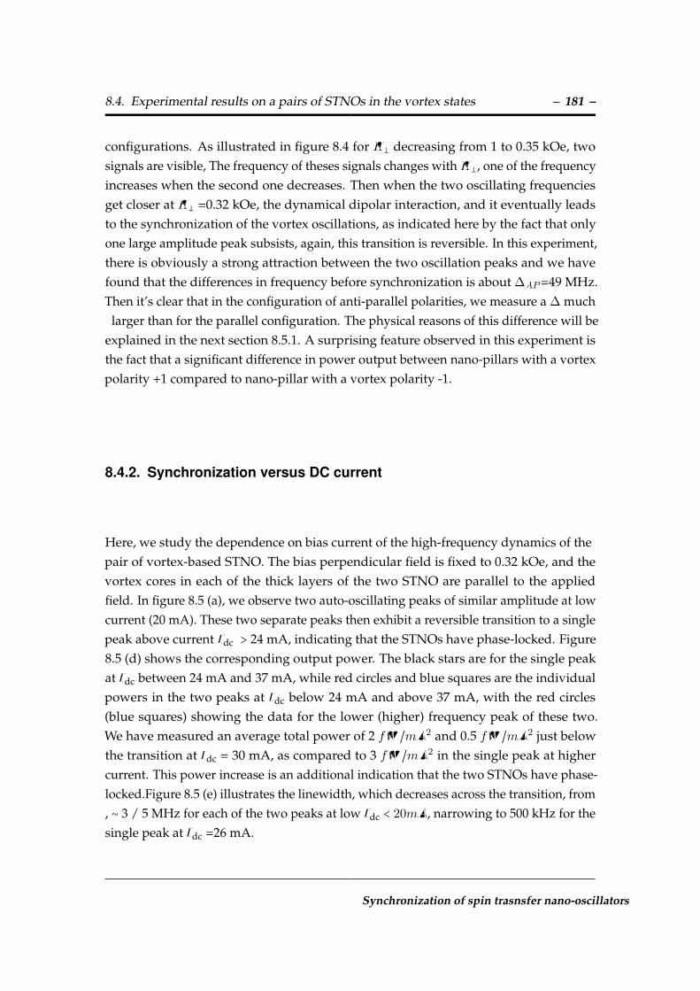
8.4. Experimental results on a pairs of STNOs in the vortex states – 181 –
configurations. As illustrated in figure 8.4 for H⊥ decreasing from 1 to 0.35 kOe, twosignals are visible, The frequency of theses signals changes with H⊥, one of the frequencyincreases when the second one decreases. Then when the two oscillating frequenciesget closer at H⊥ =0.32 kOe, the dynamical dipolar interaction, and it eventually leadsto the synchronization of the vortex oscillations, as indicated here by the fact that onlyone large amplitude peak subsists, again, this transition is reversible. In this experiment,there is obviously a strong attraction between the two oscillation peaks and we havefound that the differences in frequency before synchronization is about ∆AP=49 MHz.Then it’s clear that in the configuration of anti-parallel polarities, we measure a ∆ much
larger than for the parallel configuration. The physical reasons of this difference will beexplained in the next section 8.5.1. A surprising feature observed in this experiment isthe fact that a significant difference in power output between nano-pillars with a vortexpolarity +1 compared to nano-pillar with a vortex polarity -1.
8.4.2. Synchronization versus DC current
Here, we study the dependence on bias current of the high-frequency dynamics of thepair of vortex-based STNO. The bias perpendicular field is fixed to 0.32 kOe, and thevortex cores in each of the thick layers of the two STNO are parallel to the appliedfield. In figure 8.5 (a), we observe two auto-oscillating peaks of similar amplitude at lowcurrent (20 mA). These two separate peaks then exhibit a reversible transition to a singlepeak above current Idc > 24 mA, indicating that the STNOs have phase-locked. Figure8.5 (d) shows the corresponding output power. The black stars are for the single peakat Idc between 24 mA and 37 mA, while red circles and blue squares are the individualpowers in the two peaks at Idc below 24 mA and above 37 mA, with the red circles(blue squares) showing the data for the lower (higher) frequency peak of these two.We have measured an average total power of 2 fW /mA2 and 0.5 fW /mA2 just belowthe transition at Idc = 30 mA, as compared to 3 fW /mA2 in the single peak at highercurrent. This power increase is an additional indication that the two STNOs have phase-locked.Figure 8.5 (e) illustrates the linewidth, which decreases across the transition, from, ∼ 3 / 5 MHz for each of the two peaks at low Idc < 20mA, narrowing to 500 kHz for thesingle peak at Idc =26 mA.
Synchronization of spin trasnsfer nano-oscillators

– 182 – 8. Dipolar coupling between adjacent STNOs
Figure 8.5.: Mutual synchronization in a pair of STNOs versus current. (a) Power spectrumPSD versus frequency and applied current bias Idc for perpendicular magnetic field of 0.32 kOeand when the vortex core polarities in the two Permalloy layers are parallel. Two peaks wereobserved at Idc below 24 mA and above 40 mA, and only a single peak was observed for Idcbetween 24 and 40 mA.(c), (d) and (e) frequency, power and linewidth versus Idc. The data belowand above the synchronization is given by the red circles and blue squares. Black stars showthe data for the single peak observed. The transition from two peaks to one are accompaniedby an increase in the power and reduction in linewidth, indicating that mutual synchronizationbetween the pair STNOs has occurred.
Abbass HAMADEH
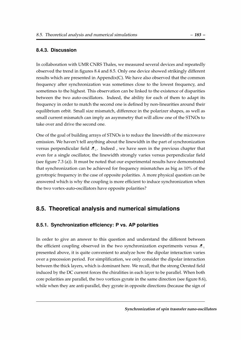
8.5. Theoretical analysis and numerical simulations – 183 –
8.4.3. Discussion
In collaboration with UMR CNRS Thales, we measured several devices and repeatedlyobserved the trend in figures 8.4 and 8.5. Only one device showed strikingly differentresults which are presented in Appendix(C). We have also observed that the commonfrequency after synchronization was sometimes close to the lowest frequency, andsometimes to the highest. This observation can be linked to the existence of disparitiesbetween the two auto-oscillators. Indeed, the ability for each of them to adapt itsfrequency in order to match the second one is defined by non-linearities around theirequilibrium orbit. Small size mismatch, difference in the polarizer shapes, as well assmall current mismatch can imply an asymmetry that will allow one of the STNOs totake over and drive the second one.
One of the goal of building arrays of STNOs is to reduce the linewidth of the microwaveemission. We haven’t tell anything about the linewidth in the part of synchronizationversus perpendicular field H⊥. Indeed , we have seen in the previous chapter thateven for a single oscillator, the linewidth strongly varies versus perpendicular field(see figure 7.3 (a)). It must be noted that our experimental results have demonstratedthat synchronization can be achieved for frequency mismatches as big as 10% of thegyrotropic frequency in the case of opposite polarities. A more physical question can beanswered which is why the coupling is more efficient to induce synchronization whenthe two vortex-auto-oscillators have opposite polarities?
8.5. Theoretical analysis and numerical simulations
8.5.1. Synchronization efficiency: P vs. AP polarities
In order to give an answer to this question and understand the different betweenthe efficient coupling observed in the two synchronization experiments versus H⊥presented above, it is quite convenient to analyze how the dipolar interaction variesover a precession period. For simplification, we only consider the dipolar interactionbetween the thick layers, which is dominant here. We recall, that the strong Oersted fieldinduced by the DC current forces the chiralities in each layer to be parallel. When bothcore polarities are parallel, the two vortices gyrate in the same direction (see figure 8.6),while when they are anti-parallel, they gyrate in opposite directions (because the sign of
Synchronization of spin trasnsfer nano-oscillators

– 184 – 8. Dipolar coupling between adjacent STNOs
Figure 8.6.: Mutual dipolar coupling mechanism. (a) Sketches showing the evolution of thedipolar coupling over a precession period in a pair of adjacent disks in the vortex state havingparallel and anti-parallel core polarities. The sign of the mutual interaction is displayed on eachside of the sketches. (b) Calculation of the dynamical stray field averaged over a precessionperiod in both cases, as a function of the gyration radius of the vortex core. The red and bluedashed lines correspond to the amplitudes of the microwave field indicated in figure 1(b).
gyrovector G is opposite, see equation 1.16). These two situations are not equivalent:contrary to the latter case, the dipolar interaction is not always minimized in the formercase, as depicted by “+” and “-” signs in figure 8.6 (a) . Therefore, the dipolar interactionaveraged over one period of precession is larger when the core polarities are anti-parallel,which should then favor synchronization.
Figure 8.7.: Dipolar energy (Wint) evolution of two interacting dipoles. The blue curve showsthe evolution of the in phase oscillating regime (parallel polarities) and the red one the anti-phasecase (anti-parallel polarities). The dashed colored lines represent the corresponding mean valueof the coupling energies. The coupling is 3 times stronger for the anti-phase oscillating case.
Abbass HAMADEH

8.5. Theoretical analysis and numerical simulations – 185 –
Now to be quantitative and to explain why the coupling isthree times more efficient toinduce synchronization when the two vortex-auto-oscillators have different polarities,and are hence gyrating in opposite directions, it is possible to calculate the dynamicalstray field averaged over a precession period in both cases, as a function of the gyrationradius of the vortex core (see figure 8.6 (b)). As seen in figure 8.6 (b) the mean dynamicalstray field is 3 times larger for anti-parallel case than that for the parallel one for a radiusgyration of 40 nm. It is also possible to calculate the interaction energy (Wint) betweenthese two configurations by using a macro-dipole approximation (see equation (8.3)).As seen graphically in figure 8.7 the mean interacting energy is three times larger for theanti-phase (red) oscillating case than for the in phase one (blue).
8.5.2. Theoretical modeling
The general theoretical modeling and numerical study of phase locking dynamics ofdipolarly coupled vortex-based spin transfer nan-oscillators, is presented in details inreferences [178, 180] and in the thesis of Nicolas Locatelli [80]. Below, we briefly recallthe general idea of this model.
The global interaction between the two vortices is very complex as it includes thecontributions from the in-plane (body) and out-of-plane (core) magnetizations. Asalready stated, the shallow dynamics of the thin 4 nm layers can be neglected, and willnot substantially contribute to the coupling. Moreover, since the size of the core is verysmall compared to the dot size (of the order of the exchange length), the dominatinginteraction is the one between the in-plane magnetizations of the thick 15 nm layers.As the vortex is gyrating, its mean in-plane magnetization describes a full rotation. Wewill then consider a simple model of two rotating macro-dipoles at the disks centerpositions. In the following, we will cautiously consider all the polarities and chiralitiesconfiguration, as P1 and C1 will relate to the first STNO and P2 and C2 to the secondone.
The proposed model is based on coupled Thiele equations. As we have shown previouslythe so called Thiele equation is a collective variable equation describing the whole vortexself-sustained gyrotropic motion through the motion of the vortex core. In the followingset of equations, a supplementary term was added to account for the dipolar coupling:
Ð→G1,2 ×
Ð→X1,2 − k1,2(X1,2)
Ð→X1,2 −D
Ð→X1,2 +
Ð→F STT +
Ð→F int = 0 . (8.1)
Synchronization of spin trasnsfer nano-oscillators

– 186 – 8. Dipolar coupling between adjacent STNOs
In these equations and for each auto-oscillator:Ð→X i is the vortex core position (both
vortices are considered centered at equilibrium positionÐ→X i= 0) ;
Ð→Gi = −PiGÐ→ez =
−2πPiLMs
γÐ→ez is the vortex gyrovector (L: layer thickness, Ms saturation magnetiza-
tion, γ : gyro-magnetic ratio) ; Wi(Ð→X i) = 1
2kiX2i is the shifted vortex energy, with
ki(Xi) = ωi0G(1 + ai(Xi/R)2) including both the magneto-static and the Oersted field
contributions (R : pillar radius); −DÐ→X1,2 withD = −αηG is the damping force accountingfor the dissipative phenomena opposing the motion (α: Gilbert damping coefficient,η = 1
2 lnR2b −
18 : damping factor, b: vortex core radius) ;
Ð→F STT accounts for the total
spin-transfer force acting on the vortex andÐ→F int = ∂Xint
∂Ð→X i
accounts for the dipolar interac-tion.
Ð→F STT = −PiλJÐ→eχ. In the specific case of a vortex polarizer [80], it was demonstratedthat the spin transfer force acting on the gyrating vortex is constant as a function ofgyration radius. As a consequence, it is not expected to have significant influence on thesynchronization process.
In a first approximation, the net in-plane magnetization of the shifted vortex growslinearly as a function of the core distance to the center of the dot : µ0Mi = Ciξ(
Ð→X i ×Ð→ez)
where ξ= 2/3 is determined analytically [34]. In a simple macro-dipole model, theinteraction energy can be expressed as :
Wmdint = V 2(
Ð→M1 ⋅
Ð→M2
D312
− 3(Ð→M1 ⋅Ð→D12)(
Ð→M2 ⋅
Ð→D12)
D512
) (8.2)
= C1C2( − µ(+)X1X2cos(ϕ1 − ϕ2) + µ(−)X1X2cos(ϕ1 + ϕ2)) (8.3)
where (X1, ϕ1) and (X2, ϕ2) are the polar coordinates of the first and second vorticescores respectively, and
Ð→D12 is a vector connecting the two dots centers. The coupling
coefficient then rewrites as µ(+) = 12ξ2V 2
D312
< 0 and µ(−) = 32ξ2V 2
D312
> 0 so that µ(−) = 3µ(+)
At this point, it must be emphasized that the gyration direction of the vortex oscillatoris governed by its core direction (polarity). As a major consequence, the contributionof the two terms to the interaction energy will be dramatically different as the polarityare identical or opposite. To account for this, we rewrite the phase evolution for thetwo auto-oscillators as : ϕ1,2 = P1,2ω1,2t + ϕi0 where ω1,2 > 0. This reveals that the firstterm associated to µ(+) oscillates in time at a frequency P1ω1,2 −P1,2ω2 where the second
Abbass HAMADEH

8.5. Theoretical analysis and numerical simulations – 187 –
one associated to µ(−) oscillates at a frequency P1ω1,2 − P1,2ω2. For two STNOs withclose frequencies ω1 ∼ ω2 , depending on the relative polarities, one term will beatat high frequency while the other will be slowly varying in time as compared to theoscillators’ gyrotropic frequencies. When considering the phase locking dynamics forsynchronization, only the slowly varying term will contribute as the second one will beaveraged out. For identical polarities, only the µ(+) term remains, when the µ(−) termremains for opposite polarities.
The two cases are illustrated on figure is the ideal condition of frequency lockingω1 = ω2 = ω. When the vortices gyrates in the same direction (identical polarities),the interaction energy shows large oscillations at frequency 2ω around a mean energy⟨Wint⟩ ∣P= −µ(+)X1X2, whereas when they gyrate in opposite direction (opposite po-larities) the interaction energy varies with lower amplitude but has a mean energy⟨Wint⟩ ∣A P = −µ(−)X1X2, three times lower. From this study it also appears that thesign of relative chiralities, despite changing the sign of the interaction coefficient, willnot affect its amplitude. Such change in the sign of the coupling will simply affect thesynchronization equilibrium phase, being whether close to ∆ϕ = 0 or π. Then, in thefollowing, we will focus on the case of identical chiralities C1C2 = +1. Starting fromthe coupled equations, we then study the synchronization phenomenon by derivingthe dynamics of the signed phase shift Ψ = P1ϕ1 − P2ϕ2. Under the assumption ofrelatively small disparities between the two oscillators and small coupling, its evolutioncan be summarized by the differential equation (see Nicolas thesis for details of thecalculation):
Ψ = ∆ω − 2µ±αη
sinΨ , (8.4)
where µ(±) stands for µ(+) in case of identical polarities and µ(−) in case of oppositepolarities. This equation is similar to the well-known Adler equation for the synchro-nization of coupled oscillators [124]. A stable equilibrium phase-shift can only exist atthe condition:
∆ω < 2µ±αη
. (8.5)
Synchronization of spin trasnsfer nano-oscillators

– 188 – 8. Dipolar coupling between adjacent STNOs
8.5.3. Discussion
This analytical result and the experimental measurements appear to be in good agree-ment, the critical frequency difference for synchronization being three times bigger in thecase of identical polarities than in the case of identical ones. However, it must be notedthat this model does not take into account the influence of the temperature. Thermalnoise can indeed reduce the synchronization region or even prevent the synchronizationif the coupling is too weak when pillars are too far away from each other. To get a hint ofthe limitation of dipolar coupling to achieve the synchronization of STNOs, we present anumerical evaluation of the mean interaction [178]. On figure 8.8 we plot the mean inter-action energy between two identical vortex auto-oscillators with diameter 200 nm as afunction of the center-to-center distance, extracted from full micro-magnetic simulations[178]. These values are extracted by studying the synchronization dynamics betweenthe two identical oscillators at zero temperature and zero field, hence with no frequencydifference. This specific case allowed us to monitor the synchronization phenomenonwhatever the amplitude of the coupling. In the figure 8.8, we identify again the factorthree between P and AP polarities cases, and can compare both associated energies tothe thermal energy at room temperature. It confirms that for a 100 nm inter-dots distance(D12 = 300nm), coupling energy is high enough to overcome thermal energy, allowingto observe synchronization in both AP and P polarities configurations. But, it appearsthat when edge-to-edge distance exceeds the pillar diameter, thermal fluctuation mayprevent synchronization, starting with the less efficient P configuration.
Abbass HAMADEH

8.6. Conclusion – 189 –
Figure 8.8.: Absolute values of interaction energy Wint as a function of inter-dot separationdistance D12 = 2R +L obtained from the micro-magnetic simulations (dots) and from the macro-dipole model (line) in the case for parallel polarities (blue) and opposite polarities (red).
8.6. Conclusion
We have investigated the synchronization of spin transfer nano-oscillators that areinteracting through dynamical dipolar coupling. We have experimentally measureda system composed of two STNOs with diameter 200 nm separated by a L=100 nmedge-to-edge distance. In this experiment, both pillars are supplied through the sameelectrodes and the current flowing in each pillar cannot be tuned independently.
We have observed that when the frequencies of the two oscillators are brought closer,they eventually merge into a single peak, demonstrating the first experimental syn-chronization through magneto-dipolar coupling. Reproducing the experiment, wemeasured and compared the experimental values of the synchronization range forcore polarities being parallel or anti-parallel. A good agreement is demonstrated be-tween experiments and analytical/numerical predictions. Namely, the coupling effi-ciency and the associated locking-range is tripled when the interacting vortices haveopposite polarities instead of identical ones. Combined with the control of vortexpolarities, this work open the path for coupling control of interaction in networks ofoscillators, which can be of great interest in applications.
Synchronization of spin trasnsfer nano-oscillators

– 190 – 8. Dipolar coupling between adjacent STNOs
Abbass HAMADEH

Conclusion and perspectives
General summary
The main goal of this thesis was to contribute to a better understanding of the microwaveproperties of STNOs, a prerequisite to optimize their performance in particular in termsof tunability by a current and spectral purity at the level of single device or severalmutually coupled oscillators. My studies have focused on two classes of configurationswhich are characterized by different excitation modes that lead to different frequencyranges and dynamic properties. The first configuration is the normally magnetizedstate of a circular nanopillar. I have studied the spin transfer driven excitation modeswhen the magnetization of both layers are out-of-plane, saturated by a strong externalmagnetic field H⊥. I have also investigated another important configuration of thesame device, which is the double vortex state. I have focused on the lowest energymode excited by spin transfer which is the coupled gyrotropic mode where the vortexcores in each magnetic layer are orbiting on a circular trajectory around the equilibriumposition.
Our first original contribution was to identify the nature of the auto-oscillating mode ina spin transfer nano-oscillator. The spectroscopic identification of the auto-oscillatingmode is usually a challenge, as a large variety of dynamic modes can be excited in STNOs,and their nature can change depending on the geometry, magnetic parameters and biasconditions. Thus, an accurate identification has important consequences regarding the
191

– 192 – Conclusion and perspectives
optimization of the performance of STNOs, because it allows to understand the detailssymmetry of the mode. The MRFM was of great interest for this identification since itcan directly monitor the power emitted by our archetype STNO. In the first step, we havestudied our STNO in the most simple configuration: a nanopillar saturated by a strongmagnetic field applied along its normal. Then from the power behavior in the sub-criticalregion of the autonomous dynamics, we have obtained a quantitative measurement ofthe threshold current and of the noise level. Their field dependence directly yields boththe spin torque efficiency acting on the thin layer and the nature of the mode whichfirst auto-oscillates: the lowest energy, spatially most uniform spin-wave mode. Fromthe MRFM behavior in the forced dynamics, it is then demonstrated that in order tophase-lock this auto-oscillating mode, the external source must have the same spatialsymmetry as the mode profile, i.e., a uniform microwave field must be used rather thana microwave current flowing through the nanopillar.
The influence of broken the axial symmetry of the perpendicular field on the auto-oscillating mode was also investigated. Interestingly, we have measured excitations in aSTNO nanopillar, revealing the occurrence of the two-mode generation regime. Thesetwo modes were identified as the lowest energy spin-wave eigen-modes of the freelayer with different azimuthal numbers ` = 0 and ` = +1. Then, we have experimentallydemonstrated that these two mode can be phase-locked to an external source havingthe appropriate symmetry. As one of these two modes is synchronized to the externalsource, the emission characteristics of the other one are also strongly affected, which canbe understood in terms of the mutual non-linear interaction between the two modes. Inparticular, a reduction of the linewidth by a factor up to five was observed on the ` = 1
mode when the mode ` = 0 was phase locked. Nevertheless, a full theoretical descriptionof this phenomenon is missing at this time.
We have then taken the advantage of the sample design to investigate the microwavecharacteristics of the same spin transfer nano-oscillator (STNO) based on coupled vor-tices as a function of the perpendicular magnetic field H⊥. Interestingly, we foundthat our vortex-based oscillator is quasi-isochronous independently of H⊥ and for aDC current ranging between 18 and 25 mA. It means that the severe nonlinear broad-ening usually observed in STNOs can be suppressed on a broad range of bias. Stillthe generation linewidth displays strong variations on H⊥ (from 40 kHz to 1 MHz),while the frequency tunability in current remains almost constant (≃ 7 MHz/mA). Thisdemonstrates that isochronicity does not necessarily imply a loss of frequency tunability,which is here governed by the current induced Oersted field. It is not sufficient either
Abbass HAMADEH

Conclusion and perspectives – 193 –
to achieve the highest spectral purity in the full range of H⊥. We have shown that theobserved linewidth broadenings are due to the excited mode interacting with a lowerenergy overdamped mode, which occurs at the successive crossings between harmonicsof these two modes. These findings open new possibilities for the design of STNOs andthe optimization of their performance. In fact, our tunability is almost ∼ 8MHz/mA atH⊥ = 0.7kOe, the sweet point for spectral purity (see Fig. 2), which corresponds to about200 times the linewidth in 1 mA.
From a practical point of view, it was demonstrated that the microwave signal generatedby a STNO based on coupled vortices can be efficiently synchronized to an external mi-crowave field. The relative locking range indeed exceeds 10% for small drive amplitudes(hrf ≃ 5 Oe) and the auto-oscillation signal acquires the spectral purity of the source, cor-responding to an improvement of its coherency by a factor greater than 105. Moreover,this perfect phase-locking is robust, as it survives even when the external frequencydeviates from the oscillator frequency by more than ten times of its linewidth.
The last main achievement of this thesis is the demonstration of the synchronizationof two STNOs coupled by the dipolar interaction. We have observed that when thefrequencies of the two oscillators are brought closer, they eventually merge into asingle peak, demonstrating the first experimental synchronization through magneto-static coupling. Reproducing the experiment, we have measured and compared theexperimental values of the synchronization range for core polarities being parallel oranti-parallel. A good agreement was demonstrated between the experiment results andthe analytical/numerical predictions. Namely, the coupling efficiency and the associatedlocking-range is tripled when the interacting vortices have opposite polarities instead ofidentical ones. Coupled to already demonstrated control of vortex polarities, this workopen the path for coupling control of interaction in networks of oscillators, which is ofgreat interest for many applications.
Outlook
From this thesis, a novel approach can be proposed to tackle the issue of spectral puritywhich is to focus on spin transfer induced collective or coupled magnetic excitations formicrowave generation in particular in the vortex state. It can be done by using advancedmultilayers made of magnetic/non magnetic stacks where consecutive ferromagneticlayers are coupled via exchange, dipolar fields and spin momentum transfer. Further
Synchronization of spin trasnsfer nano-oscillators

– 194 – Conclusion and perspectives
improvement of the microwave performance will be expected via dipolar couplingof individual spintronics devices in an array. Indeed, some important knowledgeof fundamental physics on device level was acquired in this thesis, like the role ofthe coupling mechanisms and coupling strengths between two oscillators. After ourexperimental observation, we believe that the dipolar coupling mechanism betweenindividual STNOs should be efficient to synchronize N STNO. This can expand thepossible applications of spintronics devices e.g. associative memories [177].
Finally, I hope that the knowledge gaps presented in this thesis will be filled by progress-ing in understanding the fundamental mechanisms governing the microwave propertiesin STNOs. Moreover, there are many other systems in which spin momentum transfershould generate new physics and applications [181]. In particular, it was demonstratedto be very interesting in diverse situations : chaos [182], droplet solitons [183], skyrmions[184, 185], pure spin currents [186, 187], and magnetic insulators [188].
Abbass HAMADEH

Appendices
195


APPENDIX A
Differential phase diagrams
In this appendix, we show experimental phase diagrams, with better signal to noise ratioof the MRFM and transport data. To improve the measurements, we add to Idc a smallsignal of amplitude Ipp = 0.1 mA modulated at the frequency of the cantilever, then it ispossible to measure by MRFM the small variation dMz/dI induced by this modulationand we have used a lock-in to detect the differential resistance dV /dI simultaneously.The obtained phase diagrams, presented in figure A.1 (a), look like the derivative of thosepresented in chapter 6 (see figure 6.3). Here we have measured these phase diagramsin the exact perpendicular configuration θH = 0 and at θH = 2 where θH represent theangle between the external magnetic field and the normal to the free layer. Using theconversion from MRFM data to resistance, we can also quantitatively compare MRFMto transport measurements. Two striking features can be observed in these diagrams.First, the succession of sharp peaks in dV /dI and dMz/dI , which indicate a succession ofsteps in Rdc and Mz . Second, the qualitative difference between θH = 0 and at θH = 2 inthe region of onset of the auto-oscillations: there is a peak atθH = 2 (see white arrows),absent at θH = 0 .
The succession of sharp peaks should be related to the frequency jumps of the auto-oscillations observed in the transport spectrum analyzer data see figure 6.8. Rather
197

– 198 – A. Differential phase diagrams
than a smooth opening of the precession angle in the thin layer as the supercriticalityincreases, we observe successive jumps, where the precession angle abruptly increases.This is not only observed at θH = 2 , but also at θH = 0 (where no SA data are available).However, when the supercriticality is small (ξ < 1.5), we do observe a quite smoothincrease of resistance and ∆Mz at θH = 0 (whose detailed analysis have been alreadypresented in chapter 6) and is related to the axcitation of a bi-modal regime when θH = 2,contrary to the case θH = 2. This qualitative difference was already pointed out in thediscussion in chapter 6. In figure A.1, one can also note that whereas the thresholdcurrent monotonously increases with the bias field at θH = 0, it first decreases at θH = 2,before it starts to increase above 9.6 kOe (white arrows).
Figure A.1.: Differential phase diagrams obtained at θH = 0 (top row) and at θH = 2 (bottomrow). The peak-to- peak current amplitude is Ipp = 0.1mA. The left column shows the rawMRFM data, the middle one, its conversion into differential resistancedV /dI , and the right one,the measured dV /dI using a lock-in amplifier.
Abbass HAMADEH

APPENDIX B
STNO power at large positive current
In this appendix we display the measurement of the STNO ∆Mz/Ms versus high (posi-tive and negative) current, measured by MRFM for a bias fieldH⊥ = 10 kOe. In fact, wefind that the spin-transfer torque can also excite the magnetic thick layer in our STNOfor large positive current. One can see that in region (1) (red), the current starts excitingthe precession of the thick layer. As a small precession angle opens, the ∆Mz increasesslightly (the MRFM signal starts to smoothly increase). Notice that since the criticalcurrent depends on the thickness of the layer (see equation 1.9 in chapter 1), then for thethick layer the critical at this field is about 22 mA which is ∼ 4 times greater that for thethin layer.
199
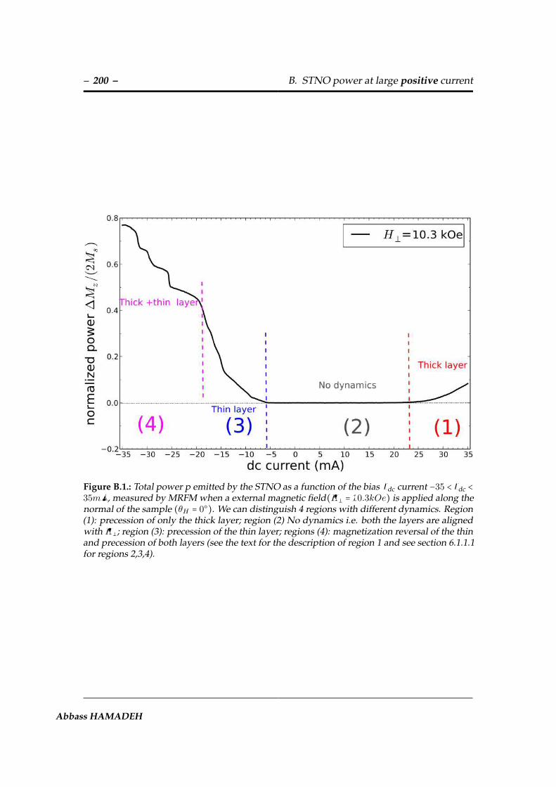
– 200 – B. STNO power at large positive current
Figure B.1.: Total power p emitted by the STNO as a function of the bias Idc current −35 < Idc <35mA, measured by MRFM when a external magnetic field(H⊥ = 10.3kOe) is applied along thenormal of the sample (θH = 0). We can distinguish 4 regions with different dynamics. Region(1): precession of only the thick layer; region (2) No dynamics i.e. both the layers are alignedwith H⊥; region (3): precession of the thin layer; regions (4): magnetization reversal of the thinand precession of both layers (see the text for the description of region 1 and see section 6.1.1.1for regions 2,3,4).
Abbass HAMADEH

APPENDIX C
Strongly mutually coupled oscillators
In this appendix, we show intersting results of mutual synchronization in a pair ofSTNOs obtained in one device which is taken from the same batch of samples (seesection 5.1.2).
In the first experiment, a constant DC current of 35 mA is applied through the device,i.e. about 17.5 mA in each STNO. The top panel of figure C.1 shows the evolutionof the auto-oscillation peaks measured on the spectrum analyzer as a function of theperpendicular applied magnetic field. Here we purposely prepared a state where thevortex core polarities in the thick layers of each STNO are opposite. We can clearly seethat when the auto-oscillation peaks are close enough in frequency, a strong pullingoccurs, that makes them meet each other (synchronize). The frequency of each oscillatoris analyzed in the bottom graph, where the data (in red) correspond to the synchronizedregime. Contrary to what is observed in figure 8.4 of chapter 8, the synchronizationin this case is not accompanied by a jump of the frequencies. It is instead close to thesynchronization phenomena observed in the pair of nano-contacts see figure 3.7 (a) ofchapter 3. One can also note the appearance of signals at mixing values of the twooscillating frequencies in the pulling regime at field above -0.9 kOe (before the vortices
201

– 202 – C. Strongly mutually coupled oscillators
Figure C.1.: (a) PSD map of a pair of STNOs separated from center to center by 300 nm. Themap are recorded as a function of the perpendicular bias magnetic field for a common currentIdc = 35 mA injected through the two STNOs in parallel. Strong mutual synchronization isobserved when the vortex core polarities in the thick layers are anti-parallel. (b) Device signalfrequency as a function of magnetic field.
phase-lock their motion). This is also observed when we synchronize a single vortexSTNO to an external source (the rf field produced by an external microwave antenna).
In addition, we have also studied the dependence on bias current of the high-frequencydynamics of this device. In this experiment the bias perpendicular field is fixed to H⊥= 1kOe, and the vortex cores in each of the thick layers of the two STNOs are parallel to theapplied field. At low current ( 14 mA), one can observe two auto-oscillating peaks ofsimilar amplitude. As the current increases, the frequencies of both oscillators increase.As both STNOs are not exactly similar (or the bias DC current that flows in each of themis slightly uneven), it happens that the two oscillator frequencies can cross each other.The crossing observed in this case is not accompanied by any pulling or jump of the two
Abbass HAMADEH

– 203 –
Figure C.2.: Power spectrum PSD versus frequency and applied current bias Idc for perpendic-ular magnetic field of 1 kOe and when the vortex core polarities in the two thick Permalloylayers are parallel. (b) and (c) Linewith and power versus Idc. The data below and above thesynchronization is given by the red circles and blue squares. Black stars show the data for thesingle peak observed. The transition from two peaks to one are accompanied by an increase inthe power and reduction in linewidth.
frequencies, in contrary to what was observed in the previous experiment (see figure8.5 of chapter 8). Here, the phase-locking manifests itself by a strong reduction of thelinewidth (see figure C.2 (c) ) and by a large increase of the amplitude (see figure C.2(b)).
Finally we have performed a measurement versus the in-plane magnetic field angleθ∡. In this experiment an external magnetic field of small constant magnitude (30 Oe)is applied to the sample at an angle θ∡ with respect to the axis through the center ofboth STNOs. As explained in section 8.4 that when we change θ∡ we can change thecoupling between the layers, and the frequency of each oscillator because the vortexcores are displaced in the magnetic layers. Figure C.3 shows the angular dependenceof the microwave spectrum at a constant current Idc = 24 mA. We observe two distinctsignals for θ∡ = 0. The frequencies of these two signals differ by about 20 MHz, andthen start to approach each other up to an angle θ∡ = 50 where the lower frequencysignal disappears, which is probably the signature of synchronization. The two distinctsignals appear again for values of θ∡ = 100 but now the two signals differ in frequenciesby only about a few MHz. It’s clear that the coupling strength is changed and for this
Synchronization of spin trasnsfer nano-oscillators

– 204 – C. Strongly mutually coupled oscillators
Figure C.3.: Map of power spectrum amplitude versus frequency and an applied in plane fieldangle θ∡ at Idc = 24 mA and Hext = 30 Oe.
angle (θ∡ = 100) the value of the coupling strength should be very small. Finally thegeneral behavior of the dependence of the microwave frequencies (two signals, onesignal) is “pseudo-periodic” with increasing the value of θ∡. The important informationthat we can conclude here that it’s possible toadjust the couplings between the STNOsby changing the in plane angle of the external magnetic field.
Discussion
The features of the mutual synchronization observed in this device are very differentfrom the one presented in chapter 8. We believe that the particular double STNO devicepresented in this appendix might have major nano-fabrication defects. Maybe the twonano-pillars are touching each other, and have quite different shapes, as supported bythe large frequency difference (> 200MHz) observed at H⊥ ∼ 0 kOe in figure C.1
Abbass HAMADEH

APPENDIX D
Pair STNOs in the saturated state
Mutual synchronization of devices with pair of STNOs was not observed in the saturatedstate. In contrast, pairwise synchronization was seen in vortex state. Figure D.1 showsthe measured frequency spectrum versus Idc in the saturated state for the same devicewhich was presented in chapter 8 (2 nano-pillars with diameter 200 nm and edge-to-edgespacings of 100 nm). The data in this measurement was taken at a magnetic field of 8kOe applied perpendicular to the plane of the sample. In Figure D.1 (a), we observethe onset of one auto-oscillation peak for Idc = -18 mA followed by a second peak ofcomparable amplitude for Idc = -20 mA. Then, the two peaks evolve nearly parallelin frequency versus Idc. For negative current it was identified that the dynamics herecorresponds to the precessional state of the thin layer in each oscillator. One can also seefrom figure D.1 that the gap in frequency between the two oscillator is about∼ 1.5 GHzwhich is much larger than observed in the vortex state (< 50 MHz). Thus, the strength ofthe dipolar interaction between the two thin layers (a few tens of MHz) is not sufficientto synchronize our two oscillators in the saturated state.
205

– 206 – D. Pair STNOs in the saturated state
Figure D.1.: Power spectrum map versus frequency and applied current bias Idc. Two peaks areobserved above Idc = -20 mA,then they move approximately parallel in frequency with Idc in thewhole range [-20 ; -25] mA.
Abbass HAMADEH

APPENDIX E
Resume substantiel en Francais
Introduction
Les recents progres technologiques dans la fabrication de nanostructures hybridesincorporant des materiaux magnetiques ont permis l’emergence de la spintronique. Cedomaine de recherche est base sur le degre de liberte de l’electron [1] de spin: courants despin sont generes et manipules a l’echelle nanometrique afin de parvenir a de nouvellesfonctionnalites.
Un dispositif elementaire de l’electronique de spin est constitue de deux couchesmagnetiques separees par une couche non-magnetique. Il presente l’effet demagnetoresistance geante (GMR) [2, 3], c’est que la resistance depend de l’angle re-latif entre les couches magnetiques. Aujourd’hui, cette propriete utile est largementutilise dans les capteurs magnetiques [4, 5]. L’effet inverse est un courant continu quipeut transferer moment angulaire de spin entre deux couches magnetiques separees soitpar un metal normal ou une couche mince isolante [?, 7]. Plus generalement, un courantde spin exerce sur un materiau ferromagnetique, un couple de transfert de spin, quipeut compenser l’amortissement et conduire a la destabilisation du moment magnetique[8]. Les applications pratiques sont la possibilite de controler l’information numerique
207

– 208 – E. Resume substantiel en Francais
dans les memoires magnetiques (MRAM) [9, 10] ou pour produire des signaux a hautefrequence dans a transfert de spin nano-oscillateurs (STNOs) [11, 12].
En raison de leur accordabilite, l’agilite, compacite, et integrabilite, les STNOs sont descandidats prometteurs pour diverses applications a haute frequence tels que generationde frequence [13, 14], detection de frequence [15, 16], traitement du signal [17, 18] etl’enregistrement dynamique [19, 20, 21]. En ce qui concerne les applications micro-ondes, la purete spectrale et la sensibilite de reglage sont deux caracteristiques clespour STNOs. Une particularite de ces dispositifs par rapport aux autres oscillateurs estleurs fortes proprietes non lineaires, qui sont heritees de l’equation du mouvement del’aimantation [22]. D’une part, ils conferent des proprietes interessantes pour STNOs,comme par exemple leur grande accordabilite frequence [11, 12, 13, 14]. D’autre part,elles conduisent a un elargissement severe de la generation du largeur de raie [23]: enraison du couplage phase-amplitude non lineaire, le bruit de phase de STNOs est eneffet assez grandes [24, 25], qui est le principal facteur limitant pour les applicationspratiques. Par consequent, les non-linearites affectent a la fois l’agilite et la puretespectrale d’une maniere de telle sorte que les deux quantites ne peuvent etre optimiseesde facon independante et un compromis doit etre trouve. En outre, etant les STNOssont des generateurs de micro-ondes a l’echelle nanometrique, leur puissance emise esttrees petite, typiquement de l’ordre de pico ou nano-Watts. Dans ce contexte, mutuellesynchronisation de plusieurs STNOs a ete proposee comme un moyen de reduire lebruit de phase et augmenter la puissance de ces oscillateurs [26, 22]. A ce jour, il yaquelques realisations experimentales de cette idee, bases sur des systemes specifiquesavec 2 ≤ N ≤ 4 STNOs mutuellement synchronises [27, 28, 29, 30]. Les principaleslimites dans le developpement de grands reseaux de STNOs synchronises sont: la dis-persion des proprietes dynamiques en raison des incertitudes dans le processus defabrication, la force du couplage dynamique, et sa symetrie, ce qui pourrait empecher lasynchronisation de grands reseaux. Par exemple, pour la meme raison pour laquelle lecouplage dipolaire seul ne peut pas etre responsable d’une aimantation spontanee (ferro-magnetisme), on ne peut pas construire un tableau 3D fermee remplie de synchronisationdes oscillateurs a travers le couplage dipolaire.
Ce travail de these a ete motivee pour mieux comprendre les proprietes de micro-ondesde STNOs, une prerequis si on veut optimiser leurs performances au niveau d’undispositif unique ou plusieurs oscillateurs couples entre eux. Pour atteindre cet objectif,un outil spectroscopique a ete adopte, parce que la connaissance du spectre du modespropres d’onde de spin dans les nanostructures magnetiques hybrides, leurs symetries,
Abbass HAMADEH

– 209 –
les energies, les taux de relaxation, et leurs proprietes non lineaires, est crucial dans denombreux aspects. D’un cte, les energies des ondes de spin, les taux de relaxation, etdes proprietes non lineaires determinent les frequences et les largeur du raie spectralequi peuvent emettre [22] par un STNO. D’un autre cte, la symetrie spatiale des modesdonne une idee fondamentale de leurs regles de selection (la facon dont ils se couplera des sources externes) et sur les mecanismes de couplage mutuel qui peuvent existerintra-ou inter-STNOs.
Les modes propres d’onde de spin peuvent etre consideres comme une empreinte d’unenanostructure magnetique et ils sont lies a son etat fondamental [31, 32]. En outre, enraison des interactions entre les differentes couches magnetiques dans un STNO (parexemple, l’interaction dipolaire), ces modes propres ont souvent un caractere collectif,c’est a dire, ils impliquent plusieurs couches dans l’empilement. Il ya quelques annees,il a ete montre experimentalement que le couple de transfert de spin pourrait exciter lemode gyrotropique d’un vortex magnetique [33], qui est le mode de plus basse energiede cet configuration [34]. Les largeurs de raies remarquablement etroites generation(environ 1 MHz ou moins) et la grande puissance de sortie dans le cas de jonctionstunnel magnetiques (MTJ) demontre par l’UMR CNRS/Thales en collaboration avecl’AIST (Japon) [?], sont extremement prometteur pour des application1.En parallele,il a ete realise dans le laboratoire du CEA Spintec que l’excitation des modes couplesdans JTMs standards uniformement magnetises pourrait ameliorer la largeur de raiejusqu’a un ordre de grandeur [38, 39]. Peu de temps avant le debut de cette these, monlaboratoire dans CEA/SPEC et l’UMR CNRS/Thales a combine ces deux idees pourreduire encore plus la largeur de raie d’auto-oscillation. En op erant un STNO base surdeux vortex couples dans un spin-valve nanopilier, ils ont obtenu un largeur de raiede ∆f = 46 kHz (pour une frequence genere f ≃ 780 MHz, ie. , f/∆f ≃ 17 000) [40].Important encore pour les applications, une grande coherence a ete maintenue, memea champ magnetique nul, et une grande accordabilite de la frequence sur le courantcontinu (≃ environ10 MHz / mA) a ete mesuree.
Afin de definir une strategie visant a optimiser les caracteristiques de micro-ondes (enparticulier la coherence) de STNOs individuels et a quelques efficacement plusieursSTNOs ensemble, les questions suivantes doivent etre adressees:
1. Quelle est la nature de la mode propre (s) auto-oscillant d ans un STNO?
1recemment, jusqu’a quelques micro-Watts ont ete signales dans les pilliers optimises ayant un grandrapport de magnetoresistance [36],Le faible bruit de phase en vortex JTM a egalement ete directementmesures et analyses [?].
Synchronization of spin trasnsfer nano-oscillators
– 210 – E. Resume substantiel en Francais
2. Quelle est l’influence des autres modes dans le systeme sur la largeur de raie?
3. Quelles sont les non-linearites dans le systeme? Quels sont les autres proprietespeuvent influer sur la largeur spectrale et la accordabilite?
4. Quel est le mecanisme de couplage optimal a verrouillage de phase la auto-oscillation a une source externe?
5. Quelle est la meilleure strategie pour synchroniser mutuellement plusieurs STNOsd’une maniere evolutive?
L’objectif de cette these est d’apporter des connaissances a ces differents points, avec uneattention particuliere pour comprendre les proprietes interessantes de STNOs base surdes vortex magnetiques. En particulier, l’interaction entre les differentes non-lineariteset des limitations a ce jour a ete largement etudie dans le cas de l’etat magnetise uni-formement. Le rle de la configuration magnetique et son influence sur les proprietesnon-lineaires etaient encore une question ouverte au debut de ma these.
Methode experimentale
Pour s’attaquer a ces questions ouvertes, une approche experimentale a ete suivie. Parconsequent, des etudes detaillees a haute frequence de STNOs bien caracterises doiventetre menees. Si l’on veut etre en mesure de comprendre avec suffisamment de precisionleurs proprietes a micro-ondes, il est donc important de travailler avec des echantillons
STNOs de conception simple et de haute symetrie. Alors, Les travaux ont ete concentreesur une nanopilier circulaire (de rayon R=120 nm) composee de seulement deux couchesferromagnetiques ayant des epaisseurs differentes et separees par une couche de metalnormal (NiFe15 nm—Cu10 nm—NiFe4 nm). L’echantillon est aimante par un champmagnetiques applique perpendiculairement le long de sa normale, afin de conserver lasymetrie axiale de cette STNO pour avoir une identification simplifiee de modes propresd’onde du spin [41]. De plus, le meme dispositif presente une configuration de doublevortex (avec un vortex dans chaque couche magnetiques) avec des proprietes de micro-ondes en suspens [40]. Cet echantillon, un archetype de STNO, est donc particulierementadapte pour apporter des reponses utiles aux questions soulevees par les motivations decette these. Pour etre coherent avec notre feuille de route, le meme dispositif de STNO,mais en double, sera utilisee dans les etudes de synchronisation mutuelle.
Abbass HAMADEH
– 211 –
Une originalite de ce travail est son point de vue spectroscopique. Il faut donc des outilsspectroscopiques pour etudier la dynamique de l’aimantation dans STNOs. Un moyennaturel pour sonder les modes d’onde de spin dans les nanostructures hybrides consistea utiliser les proprietes de magnetoresistance [42, 43, 44, 45, 46]. Depuis sa premiereapplication pour STNOs [11], analyse spectrale des signaux emis a repandu. Cependant,ces techniques de transport a haute frequence ne sont pas sensibles a tous les modesd’onde de spin, car certains peuvent etre caches a eux en raison de regles de selection[41]. De plus, ils ne fournissent pas un acces direct a des profils de mode spatial. Desmethodes experimentales independantes des transports ont recemment apporte desinformations utiles a la dynamique de l’aimantation dans les nanostructures hybrides[47, 48, 49, 50, 51, 52]. En particulier, les techniques optiques telles que la resolutiontemporelle magneto-optique Kerr microscopie (TR-MOKE) [53], micro Brillouin LightScattering (µ BLS) [54], ou X-ray circulaire magnetiques dichrosme (XMCD) [55] ontrecemment ete appliquee avec succes a sonder transfert de spin dynamique parcourus.Cependant, ces techniques experimentales necessiten un acces optique a la partie activede l’echantillon. cet egard, microscopie de force a resonance magnetique (MRFM)[56, 57, 58, 59, 60], qui est base sur l’interaction dipolaire entre l’echantillon et une sondemagnetique fixee a l’extremite libre d’un cantilever souple, est bien adapte a l’etude desSTNOs [41]. En fait, cette technique tres sensible permet de detecter la dynamique del’aimantation dans les nanostructures enterrees sous des electrodes metalliques epaisses[61], surtout que dans les STNOs sont couvree par des electrodes qui sont necessaire pourpasser des grandes densites de courant necessaires pour compenser l’amortissement. Parailleurs, il est sensible a tous les modes d’ondes de spin, parce qu’il mesure directementla composante longitudinale de l’aimantation ∆Mz[62].
Dans cette these, on a utilises les deux techniques de MRFM et de transport a hautefrequence pour detecter la dynamique de l’aimantation dans un STNO o dans les couchesmagnetiques soit dans le sature et ou a l’etat de vortex. Ces deux techniques apporterontdes informations complementaires pour repondre aux questions ouvertes proposeesci-dessus.
STNO dans l’etat sature
Dans cette partie nous avons etudie la dynamique d’auto-oscillations de l’aimantationdans un nano-oscillateur a transfert de spin dans l’etat sature. La technique MRFM
Synchronization of spin trasnsfer nano-oscillators
– 212 – E. Resume substantiel en Francais
nous a permis d’etudier les effets de transfert de spin dans une configuration de hautesymetrie permettant une identification simplifiee des modes propres du systeme, quandles mesures standards de transport haute fr equence ne le permettent pas. L’originalit ede notre experience est de se coupler directement a la variation d’aimantation longitudi-nale dans le nano-pilier ∆Mz , directement proportionnelle a la puissance emise par leSTNO. Cette etude d’un STNO nous a d’abord permis de definir les lignes critiques quiseparent les differents etats stables du systeme qui sont necessaires pour comprendreses proprietes dynamique (figure E.1). En particulier, une analyse quantitative du seuilcritique du mode de plus basse energie dans la couche fine a ete menee dans le cadre dumodele universel d’un auto-oscillateur a amortissement compense [22]. Ensuite, nousavons identifie le mode d’auto-oscillation dans la couche fine. En utilisant deux circuitsmicro-onde differents, nous avons pu selectivement sonder les modes d’indice `=0 et`=1 dans le nano-pilier. Les premiers sont excites par le champ micro-onde uniforme hrfgenere par une antenne, tandis que les seconds se couplent au champ d’Oersted cree parun courant micro-onde irf traversant l’echantillon. Nous avons observe une differencede comportement qualitative entre les modes `=0 et `=1 de la couche fine en fonctiondu courant continu. Les spectres MRFM du mode `=0 se distordent, avec l’apparitiond’un lobe negatif, alors que cela n’est pas observe pour le mode `=1 (figure E.2). Ceteffet est associe a la synchronisation du mode qui auto-oscille a la source externe, ici hrf: sur la gamme de phase locking, l’amplitude de ce mode s’adapte de facon a ce que safrequence reste constante et egale a celle de la source (figure). Cette observation permetde montrer que le mode auto-oscillant, qui est le mode portant l’index azimutal `=0 deplus basse energie de la couche fine, susceptible de se coupler a la symetrie uniforme de
l’excitation. Au contraire, on a observe que l’excitation par un courant ne provoque pasd’effet de synchronisation, en raison de sa symetrie azimutale (`=1) incompatible avec lemode qui auto-oscille. Dans le cas particulier de la configuration de haute symetrie quenous avons etudie, il apparat donc que le couplage dipolaire entre STNOs voisins peutetre tres efficace pour synchroniser un reseau, alors que le courant RF ne l’est pas.
STNO dans L’etat vortex
Notre oscillateur a ensuite ete etudie sous faible champ perpendiculaire. En fait, enfonction des conditions de champ magnetique applique et de courant traversant le pillier,il est possible d’y exciter une grande variete de modes magnetiques par transfert de spin.Toutefois, lorsqu’aucun champ magnetique exterieur n’est applique, les deux couches
Abbass HAMADEH
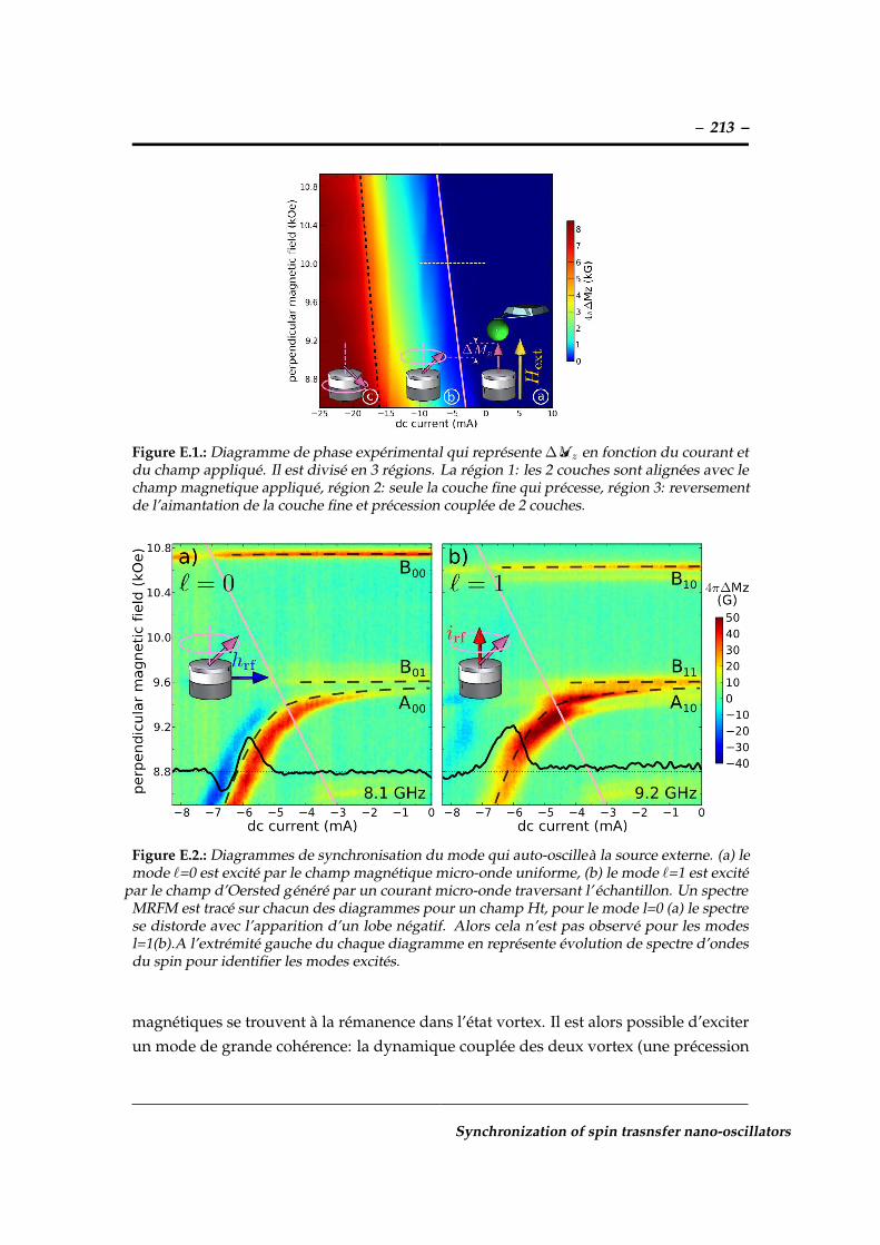
– 213 –
Figure E.1.: Diagramme de phase experimental qui represente ∆Mz en fonction du courant etdu champ applique. Il est divise en 3 regions. La region 1: les 2 couches sont alignees avec lechamp magnetique applique, region 2: seule la couche fine qui precesse, region 3: reversementde l’aimantation de la couche fine et precession couplee de 2 couches.
Figure E.2.: Diagrammes de synchronisation du mode qui auto-oscillea la source externe. (a) lemode `=0 est excite par le champ magnetique micro-onde uniforme, (b) le mode `=1 est excite
par le champ d’Oersted genere par un courant micro-onde traversant l’ echantillon. Un spectreMRFM est trace sur chacun des diagrammes pour un champ Ht, pour le mode l=0 (a) le spectrese distorde avec l’apparition d’un lobe negatif. Alors cela n’est pas observe pour les modesl=1(b).A l’extremite gauche du chaque diagramme en represente evolution de spectre d’ondesdu spin pour identifier les modes excites.
magnetiques se trouvent a la remanence dans l’etat vortex. Il est alors possible d’exciterun mode de grande coherence: la dynamique couplee des deux vortex (une precession
Synchronization of spin trasnsfer nano-oscillators
– 214 – E. Resume substantiel en Francais
couplee des coeurs de vortex appelee mode gyrotropique), induite par transfert de spin[40]. L’etat magnetique doit neanmoins etre prepare de facon a avoir deux vortex dechiralites identiques et de polarites opposees dans chacune des deux couches. Dans unepremiere etude en analysant le contenu harmonique du spectre, nous avons determineque le couplage non-lineaire amplitude-phase du mode excite est quasi nul, ce quiexplique la grande purete spectrale observee, et qu’en parallele, la frequence d’oscillationreste ajustable sur une grande gamme grace au champ d’Oersted cree par le courantinjecte. Dans une dexieme etude, nous avons concentre sur la dynamique de modecouple generer par l’oscillateur en presence d’une source exterieure. Sur la figure E.3,nous presentons une mesure effectuee sur le STNO soumis a un champ magnetiquemicro-onde alternatif uniforme d’amplitude hrf= 2.5 Oe dont la frequence Fs est balayee.Le courant injecte dans l’oscillateur est egal a 15 mA, et la frequence libre des oscillationsest Fo=585 MHz, (mode gyrotropique domine par la couche epaisse). Lorsque Fs
est suffisamment proche de Fo, l’oscillateur s’ecarte de sa frequence propre pour sesynchroniser sur la frequence de la source. On releve alors la dependance de la fenetrede synchronisation ∆ (locking range) en fonction de l’amplitude de la source, quenous presentons sur la figure E.3 (b): ∆ peut atteindre plus de 10 % de Fo pour unefaible amplitude hrf =6 Oe. On souhaite ensuite etudier l’evolution de la largeurde raie du signal releve aux bornes de l’oscillateur (caracterisant la coherence desoscillations) lors du verrouillage de phase du STNO. Cependant, il n’est pas possibled’etudier le comportement de la largeur de raie de l’oscillateur lorsque Fs=F0 car lesignal directement issu de la source masque le signal issu du STNO. Pour y remedier,nous avons etudie la synchronisation du STNO a Fs=2Fo et Fs=2Fo. La forte diminutionde la largeur de raie de l’oscillateur lorsqu’il se synchronise a la source peut alors etreobservee: pour un champ applique hors du plan de 1 kOe, la largeur de raie decroitmeme de 100 kHz a moins de 1 Hz, c’est-a-dire que le STNO se synchronise parfaitementa la source externe. Il est finalement a noter que pour des raisons de symetrie, lemode gyrotropique couple de notre STNO ne se synchronise qu’au champ uniformehrf , et pas du tout a un courant irf . Il apparat donc que de nouveau que le couplagemagneto-dipolaire entre STNOs a base de vortex est tres prometteur pour obtenir unesynchronisation mutuelle, le cham p dipolaire rayonne par un STNO sur ses voisinsjouant alors le rle de la source hrf dans cette etude.
Abbass HAMADEH

– 215 –
Figure E.3.: (a) Evolution de la frequence d’auto-oscillation en fonction de la frequence de lasource hrf = 2.5 Oe. ∆ represente le locking range. (b) Locking range en fonction de l’amplitudedu champ applique. Dans les deux cas Idc=15 mA.
Synchronisation mutuelle
Un des objectifs de cette partie est de demontrer s’il est possible d’observer unphenomene de synchronisation mutuelle entre les oscillations de deux STNOs. Nousavons pour cela realise des echantillons constitues de deux piliers de diametre D=200nmgraves dans un meme empilement de celle presenter avant et separes d’une distances=100nm bord-a-bord. Les deux STNOs sont alimentes en courant par une electrodecommune.
L’etape suivante a ete de mesurer experimentalement ce systeme de deux STNOs, dansdifferentes configurations de polarites des vortex. Sur la figure E.4, nous representonsles evolutions des caracteristiques de la frequence des deux oscillateurs en fonctiond’un champ exterieur applique selon l’axe des piliers. On peut faire varier l’ecart enfrequence des deux oscillateurs grace a l’application d’un champ perpendiculaire. Nouspresentons sur la figure E.4 (a) (figure E.4 (b)) le cas experimental de deux vortex depolarites opposees (parallele). La reduction (augmentation) du champ magnetiqueapplique permettra de reduire progressivement l’ecart en frequence jusqu’a observerle phenomene de synchronisation. En fait et nous avons pu observer le ph enomene desynchronisation dans le cas de vortex de polarites parallele et anti-paralleles En dessous
Synchronization of spin trasnsfer nano-oscillators

– 216 – E. Resume substantiel en Francais
d’un ecart en frequence de critique, les deux signaux issus de chacun des oscillateurs nefont plus qu’un : ils oscillent maintenant a la meme frequence. Ces resultats constituentla premiere demonstration experimentale a temperature ambiante de synchronisationd’oscillateurs a transfert de spin par couplage dipolaire.
Ces observations ont pu etre repetees pour plusieurs echantillons et dans differentesconfigurations des vortex. Finalement la synchronisation s’est montree etre beaucoup
plus efficace dans la configuration de polarit es opposees, pour laquelle nous avons puobserver une synchronisation pour un ecart en frequence d’environ 50 MHz, soit 8 %
de la frequence d’oscillation gyrotropique. Ce pourcentage represente potentiellementla dispersion maximale en frequence permettant d’observer la synchronisation d’uneassemblee d’oscillateurs.
Ces resultats extremement interessants ouvrent la perspective de la fabrication dereseauxd’oscillateurs spintroniques couples, qui permettront de renforcer la puissanceet la coherence des signaux dont ils seront a l’origine.
Figure E.4.: Phenomene de synchronisation Cartographie du spectre en tension aux bornes desdeux piliers, montrant le phenomene de synchronisation. Les mesures sont enregistrees enfonction du champ magnetique perpendiculaire a un courant Idc = 38 mA injecte par les deuxSTNOs en parallele. (a) Synchronisation mutuelle dans les cas pour lesquels les polarites desvortex dans la couche epaisse de Py sont anti-paralleles. (b) paralleles
Abbass HAMADEH

References
[1] S. Wolf, D. D. Awschalom, R. A. Buhrman, J. Daughton, S. von Molnar, M. L.Roukes, A. Y. Chtchelkanova and D. M. Treger, Spintronics: A Spin-Based ElectronicsVision for the Future, Science 294, 1488 (2001).
[2] M. N. Baibich, J. M. Broto, A. Fert, F. N. V. Dau, F. Petroff, P. Etienne, G. Creuzet,A. Friederich and J. Chazelas, Giant magnetoresistance of (001)Fe/(001)Cr magneticsuperlattices, Phys. Rev. Lett. 61, 2472 (1988).
[3] G. Binasch, P. Grunberg, F. Saurenbach and W. Zinn, Enhanced magnetoresistance inlayered magnetic structures with antiferromagnetic interlayer exchange, Phys.Rev.B 39,4828 (1989).
[4] B. Dieny, V. Speriosu, B. Gurney, S. Parkin, D. Wilhoit, K. Roche, S. Metin, D.Peterson and S. Nadimi, Spin-valve effect in soft ferromagnetic sandwiches, Journal ofMagnetism and Magnetic Materials 93, 101 (1991).
[5] M. Pannetier, C. Fermon, G. Le Goff, J. Simola and E. Kerr, Femtotesla MagneticField Measurement with Magnetoresistive Sensors, Science 304, 1648 (2004).
[6] J. C. Slonczewski, Current-driven excitation of magnetic multilayers , J. Magn. Magn.Mater. 159, 1 (1996).
[7] L. Berger, Emission of spin waves by a magnetic multilayer traversed by a current, Phys.Rev. B 54, 9353 (1996).
217

– 218 – References
[8] D. Ralph and M. Stiles, Spin transfer torques, Journal of Magnetism and MagneticMaterials 320, 1190 (2008).
[9] F. J. Albert, J. A. Katine, R. A. Buhrman and D. C. Ralph, Spin-polarized currentswitching of a Co thin film nanomagnet, Applied Physics Letters 77, 3809 (2000).
[10] J. Grollier, V. Cros, A. Hamzic, J. M. George, H. Jaffres, A. Fert, G. Faini, J. B.Youssef and H. Legall, Spin-polarized current induced switching in Co/Cu/Co pillars,Applied Physics Letters 78, 3663 (2001).
[11] S. I. Kiselev, J. C. Sankey, I. N. Krivorotov, N. C. Emley, R. J. Schoelkopf, R. A.Buhrman and D. C. Ralph, Microwave oscillations of a nanomagnet driven by a spin-polarized current, Nature 425, 380 (2003).
[12] W. H. Rippard, M. R. Pufall, S. Kaka, S. E. Russek and T. J. Silva, Direct-CurrentInduced Dynamics in Co90Fe10/Ni80Fe20 Point Contacts, Phys. Rev. Lett. 92, 027201(2004).
[13] D. Houssameddine, U. Ebels, B. Delat, B. Rodmacq, I. Firastrau, F. Ponthenier, M.Brunet, C. Thirion, J.-P. Michel, L. Prejbeanu-Buda, M.-C. Cyrille, O. Redon andB. Dieny, Spin-torque oscillator using a perpendicular polarizer and a planar free layer,Nature Mater. 6, 447 (2007).
[14] S. Bonetti, P. Muduli, F. Mancoff and J. Akerman, Spin torque oscillator frequencyversus magnetic field angle: The prospect of operation beyond 65 GHz, Appl. Phys. Lett.94, 102507 (2009).
[15] A. A. Tulapurkar, Y. Suzuki, A. Fukushima, H. Kubota, H. Maehara, K. Tsunekawa,D. D. Djayaprawira, N. Watanabe and S. Yuasa, Spin-torque diode effect in magnetictunnel junctions, Nature 438, 339 (2005).
[16] J. Zhu, J. A. Katine, G. E. Rowlands, Y.-J. Chen, Z. Duan, J. G. Alzate, P. Upadhyaya,J. Langer, P. K. Amiri, K. L. Wang and I. N. Krivorotov, Voltage-Induced FerromagneticResonance in Magnetic Tunnel Junctions, Phys. Rev. Lett. 108, 197203 (2012).
[17] P. K. Muduli, Y. Pogoryelov, S. Bonetti, G. Consolo, F. Mancoff and J. Akerman,Nonlinear frequency and amplitude modulation of a nanocontact-based spin-torque oscil-lator, Phys. Rev. B 81, 140408 (2010).
Abbass HAMADEH

References – 219 –
[18] Y. Pogoryelov, P. K. Muduli, S. Bonetti, E. Iacocca, F. Mancoff and J. Akerman,Frequency modulation of spin torque oscillator pairs, Appl. Phys. Lett. 98, 192501(2011).
[19] P. M. Braganca, B. A. Gurney, B. A. Wilson, J. A. Katine, S. Maat and J. R. Childress,Nanoscale magnetic field detection using a spin torque oscillator, Nanotechnology 21,235202 (2010).
[20] K. Mizushima, K. Kudo, T. Nagasawa and R. Sato, Signal-to-noise ratios in high-signal-transfer-rate read heads composed of spin-torque oscillators , Journal of AppliedPhysics 107, 063904 (2010).
[21] J.-G. Zhu and Y. Wang, Microwave Assisted Magnetic Recording Utilizing Perpendicu-lar Spin Torque Oscillator With Switchable Perpendicular Electrodes, IEEE Trans. Magn.46, 751 (2010).
[22] A. Slavin and V. Tiberkevich, Nonlinear Auto-Oscillator Theory of Microwave Genera-tion by Spin-Polarized Current, IEEE Transactions on Magnetics 45, 1875 (2009).
[23] J.-V. Kim, V. Tiberkevich and A. N. Slavin, Generation Linewidth of an Auto-Oscillatorwith a Nonlinear Frequency Shift: Spin-Torque Nano-Oscillator, Phy.Rev.Let. 100,017207 (2008).
[24] M. W. Keller, M. R. Pufall, W. H. Rippard and T. J. Silva, Nonwhite frequency noisein spin torque oscillators and its effect on spectral linewidth, Phys. Rev. B 82, 054416(2010).
[25] M. Quinsat, D. Gusakova, J. F. Sierra, J. P. Michel, D. Houssameddine, B. Delaet,M.-C. Cyrille, U. Ebels, B. Dieny, L. D. Buda-Prejbeanu, J. A. Katine, D. Mauri, A.Zeltser, M. Prigent, J.-C. Nallatamby and R. Sommet, Amplitude and phase noise ofmagnetic tunnel junction oscillators, Appl. Phys. Lett. 97, 182507 (2010).
[26] J. Grollier, V. Cros and A. Fert, Synchronization of spin-transfer oscillators driven bystimulated microwave currents, Phys. Rev. B 73, 060409 (2006).
[27] S. Kaka, M. R. Pufall, W. H. Rippard, T. J. Silva, S. E. Russek and J. A. Katine,Mutual phase-locking of microwave spin torque nano-oscillators, Nature 437, 389 (2005).
[28] F. B. Mancoff, N. D. Rizzo, B. N. Engel and S. Tehrani, Phase-locking in double-point-contact spin-transfer devices, Nature 437, 393 (2005).
Synchronization of spin trasnsfer nano-oscillators
– 220 – References
[29] A. Ruotolo, V. Cros, B. Georges, A. Dussaux, J. Grollier, C. Deranlot, R. Guillemet,K. Bouzehouane, S. Fusil and A. Fert, Phase-locking of magnetic vortices mediated byantivortices, Nature Nanotech. 4, 528 (2009).
[30] S. Sani, J. Persson, S. Mohseni, Y. Pogoryelov, P. Muduli, A. Eklund, G. Malm, M.Kll, A. Dmitriev and J. Akerman, Mutually synchronized bottom-up multi-nanocontactspin-torque oscillators, Nature Communications 4, 2731 (2013).
[31] M. Bailleul, R. Hollinger and C. Fermon, Microwave spectrum of square Permalloydots: Quasisaturated state, Physical Review B (Condensed Matter and MaterialsPhysics) 73, 104424 (2006).
[32] M. Bailleul, R. Hollinger, K. Perzlmaier and C. Fermon, Microwave spectrum ofsquare permalloy dots: Multidomain state, Physical Review B (Condensed Matter andMaterials Physics) 76, 224401 (2007).
[33] V. S. Pribiag, I. N. Krivorotov, G. D. Fuchs, P. M. Braganca, O. Ozatay, J. C. Sankey,D. C. Ralph and R. A. Buhrman, Magnetic vortex oscillator driven by d.c. spin-polarizedcurrent, Nature Phys. 3, 498 (2007).
[34] K. Y. Guslienko, Magnetic Vortex State Stability, Reversal and Dynamics in RestrictedGeometries, J. Nanosci. Nanotechnol. 8, 2745 (2008).
[35] A. Dussaux, B. Georges, J. Grollier, V. Cros, A. Khvalkovskiy, A. Fukushima, M.Konoto, H. Kubota, K. Yakushiji, S. Yuasa, K. Zvezdin, K. Ando and A. Fert, Largemicrowave generation from current-driven magnetic vortex oscillators in magnetic tunneljunctions, Nat. Commun. 1, 8 (2010).
[36] S. Tsunegi, H. Kubota, K. Yakushiji, M. Konoto, S. Tamaru, A. Fukushima, H. Arai,H. Imamura, E. Grimaldi, R. Lebrun, J. Grollier, V. Cros and S. Yuasa, High emissionpower and Q factor in spin torque vortex oscillator consisting of FeB free layer, AppliedPhysics Express 7, 063009 (2014).
[37] E. Grimaldi, A. Dussaux, P. Bortolotti, J. Grollier, G. Pillet, A. Fukushima, H.Kubota, K. Yakushiji, S. Yuasa and V. Cros, Response to noise of a vortex based spintransfer nano-oscillator, Phys. Rev. B 89, 104404 (2014).
[38] D. Houssameddine, J. F. Sierra, D. Gusakova, B. Delaet, U. Ebels, L. D. Buda-Prejbeanu, M.-C. Cyrille, B. Dieny, B. Ocker, J. Langer and W. Maas, Spin torque
Abbass HAMADEH

References – 221 –
driven excitations in a synthetic antiferromagnet , Applied Physics Letters 96, 072511(2010).
[39] D. Gusakova, M. Quinsat, J. F. Sierra, U. Ebels, B. Dieny, L. D. Buda-Prejbeanu,M.-C. Cyrille, V. Tiberkevich and A. N. Slavin, Linewidth reduction in a spin-torquenano-oscillator caused by non-conservative current-induced coupling between magneticlayers, Appl. Phys. Lett. 99, 052501 (2011).
[40] N. Locatelli, V. V. Naletov, J. Grollier, G. de Loubens, V. Cros, C. Deranlot, C.Ulysse, G. Faini, O. Klein and A. Fert, Dynamics of two coupled vortices in a spin valvenanopillar excited by spin transfer torque, Appl. Phys. Lett. 98, 062501 (2011).
[41] V. V. Naletov, G. de Loubens, G. Albuquerque, S. Borlenghi, V. Cros, G. Faini, J.Grollier, H. Hurdequint, N. Locatelli, B. Pigeau, A. N. Slavin, V. S. Tiberkevich,C. Ulysse, T. Valet and O. Klein, Identification and selection rules of the spin-waveeigenmodes in a normally magnetized nanopillar, Phys. Rev. B 84, 224423 (2011).
[42] S. Petit, C. Baraduc, C. Thirion, U. Ebels, Y. Liu, M. Li, P. Wang and B. Dieny,Spin-Torque Influence on the High-Frequency Magnetization Fluctuations in MagneticTunnel Junctions, Phys. Rev. Lett. 98, 077203 (2007).
[43] A. Helmer, S. Cornelissen, T. Devolder, J.-V. Kim, W. van Roy, L. Lagae and C.Chappert, Quantized spin-wave modes in magnetic tunnel junction nanopillars , Phys.Rev. B 81, 094416 (2010).
[44] J. C. Sankey, P. M. Braganca, A. G. F. Garcia, I. N. Krivorotov, R. A. Buhrman andD. C. Ralph, Spin-Transfer-Driven Ferromagnetic Resonance of Individual Nanomagnets,Phys. Rev. Lett. 96, 227601 (2006).
[45] W. Chen, J.-M. L. Beaujour, G. de Loubens, A. D. Kent and J. Z. Sun, Spin-torquedriven ferromagnetic resonance of Co/Ni synthetic layers in spin valves, Appl. Phys. Lett.92, 012507 (2008).
[46] N. Biziere and C. Fermon, High-frequency giant magnetoresistance measurement tostudy the dynamics of a micron-scale spin-valve sensor, Physical Review B (CondensedMatter and Materials Physics) 78, 064408 (2008).
[47] V. E. Demidov, S. O. Demokritov, B. Hillebrands, M. Laufenberg and P. P. Freitas,Radiation of spin waves by a single micrometer-sized magnetic element, Appl. Phys. Lett.85, 2866 (2004).
Synchronization of spin trasnsfer nano-oscillators
– 222 – References
[48] G. Woltersdorf, O. Mosendz, B. Heinrich and C. H. Back, Magnetization Dynamicsdue to Pure Spin Currents in Magnetic Double Layers, Phys. Rev. Lett. 99, 246603(2007).
[49] G. de Loubens, V. V. Naletov, O. Klein, J. B. Youssef, F. Boust and N. Vukadinovic,Magnetic Resonance Studies of the Fundamental Spin-Wave Modes in Individual Sub-micron Cu/NiFe/Cu Perpendicularly Magnetized Disks, Physical Review Letters 98,127601 (2007).
[50] G. Gubbiotti, M. Madami, S. Tacchi, G. Carlotti, H. Tanigawa and T. Ono, Spindynamics of multilayered nanoelements with different shapes studied by Brillouin lightscattering technique, J. Phys. D: Appl. Phys. 41, 134023 (2008).
[51] P. S. Keatley, P. Gangmei, M. Dvornik, R. J. Hicken, J. R. Childress and J. A. Katine,Large amplitude magnetization dynamics and the suppression of edge modes in a singlenanomagnet, Applied Physics Letters 98, 082506 (2011).
[52] H. T. Nembach, J. M. Shaw, C. T. Boone and T. J. Silva, Mode- and Size-DependentLandau-Lifshitz Damping in Magnetic Nanostructures: Evidence for Nonlocal Damping,Phys. Rev. Lett. 110, 117201 (2013).
[53] J.-Y. Chauleau, H. G. Bauer, H. S. Korner, J. Stigloher, M. Hartinger, G. Woltersdorfand C. H. Back, Self-consistent determination of the key spin-transfer torque parametersfrom spin-wave Doppler experiments, Phys. Rev. B 89, 020403 (2014).
[54] V. E. Demidov, M. Buchmeier, K. Rott, P. Krzysteczko, J. Munchenberger, G. Reissand S. O. Demokritov, Nonlinear Hybridization of the Fundamental Eigenmodes ofMicroscopic Ferromagnetic Ellipses, Phys. Rev. Lett. 104, 217203 (2010).
[55] Y. Acremann, J. P. Strachan, V. Chembrolu, S. D. Andrews, T. Tyliszczak, J. A.Katine, M. J. Carey, B. M. Clemens, H. C. Siegmann and J. Stohr, Time-ResolvedImaging of Spin Transfer Switching: Beyond the Macrospin Concept, Phys. Rev. Lett. 96,217202 (2006).
[56] Z. Zhang, P. C. Hammel and P. E. Wigen, Observation of ferromagnetic resonance in amicroscopic sample using magnetic resonance force microscopy, Applied Physics Letters68, 2005 (1996).
Abbass HAMADEH
References – 223 –
[57] K. Wago, D. Botkin, C. S. Yannoni and D. Rugar, Paramagnetic and ferromagneticresonance imaging with a tip-on-cantilever magnetic resonance force microscope, Appl.Phys. Lett. 72, 2757 (1998).
[58] V. Charbois, V. V. Naletov, J. B. Youssef and O. Klein, Influence of the magnetic tip inferromagnetic resonance force microscopy, Applied Physics Letters 80, 4795 (2002).
[59] O. Klein, G. de Loubens, V. V. Naletov, F. Boust, T. Guillet, H. Hurdequint, A. Lek-sikov, A. N. Slavin, V. S. Tiberkevich and N. Vukadinovic, Ferromagnetic resonanceforce spectroscopy of individual submicron-size samples, Phys. Rev. B 78, 144410 (2008).
[60] H.-J. Chia, F. Guo, L. M. Belova and R. D. McMichael, Nanoscale Spin Wave Localiza-tion Using Ferromagnetic Resonance Force Microscopy, Phys. Rev. Lett. 108, 087206(2012).
[61] G. de Loubens, A. Riegler, B. Pigeau, F. Lochner, F. Boust, K. Y. Guslienko, H.Hurdequint, L. W. Molenkamp, G. Schmidt, A. N. Slavin, V. S. Tiberkevich, N.Vukadinovic and O. Klein, Bistability of Vortex Core Dynamics in a Single Perpendicu-larly Magnetized Nanodisk, Physical Review Letters 102, 177602 (2009).
[62] G. de Loubens, V. V. Naletov and O. Klein, Reduction of the spin-wave dampinginduced by nonlinear effects, Phys. Rev. B 71, 180411(R) (2005).
[63] E. M. Landau, L. D. .and Lifshitz, On the theory of the despersion of magnetic perme-ability in ferromagnetic bodies, Sov. Phys. 8, 153 (1935).
[64] T. L. Gilbert, A lagrangian formulation of the gyromagnetic equation of the magnetizationfield, Phys. Rev. 100, 1243 (1955).
[65] K. L. Metlov and K. Y. Guslienko, Stability of magnetic vortex in soft magnetic nano-sized circular cylinder, Journal of magnetism and magnetic materials 242, 1015(2002).
[66] N. A. Usov and S. E. Peschany, Magnetization curling in a fine cylindrical particle,J.Magn.Magn.Mater. 118, L290 (1993).
[67] K. Y. Guslienko and K. L. Metlov, Evolution and stability of a magnetic vortex ina small cylindrical ferromagnetic particle under applied field, Physical Review B 63,100403 (2001).
Synchronization of spin trasnsfer nano-oscillators

– 224 – References
[68] M. Hehn, K. Ounadjela, J.-P. Bucher, F. Rousseaux, D. Decanini, B. Bartenlian andC. Chappert, Nanoscale magnetic domains in mesoscopic magnets, Science 272, 1782(1996).
[69] R. P. Cowburn, D. K. Koltsov, A. O. Adeyeye, M. E. Welland and D. M. Tricker,Single-Domain Circular Nanomagnets, Phys. Rev. Lett. 83, 1042 (1999).
[70] K. L. Metlov and K. Y. Guslienko, Quasiuniform magnetization state in soft ferromag-netic nanocylinders, Phys. Rev. B 70, 052406 (2004).
[71] K. Y. Guslienko, V. Novosad, Y. Otani, H. Shima and K. Fukamichi, Field evolution ofmagnetic vortex state in ferromagnetic disks, Applied Physics Letters 78, 3848 (2001).
[72] K. Y. Guslienko, V. Novosad, Y. Otani, H. Shima and K. Fukamichi, Magneti-zation reversal due to vortex nucleation, displacement, and annihilation in submicronferromagnetic dot arrays, Phys. Rev. B 65, 024414 (2002).
[73] A. Fernandez, M. Gibbons, M. Wall and C. Cerjan, Magnetic domain structure andmagnetization reversal in submicron-scale Co dots, Journal of Magnetism and MagneticMaterials 190, 71 (1998).
[74] S. Urazhdin, C. Chien, K. Y. Guslienko and L. Novozhilova, Effects of current on themagnetic states of permalloy nanodiscs, Physical Review B 73, 054416 (2006).
[75] A. A. Thiele, Steady-State Motion of Magnetic Domains, Phys. Rev. Lett. 30, 230(1973).
[76] A. V. Khvalkovskiy, J. Grollier, A. Dussaux, K. A. Zvezdin and V. Cros, Vortexoscillations induced by spin-polarized current in a magnetic nanopillar: Analytical versusmicromagnetic calculations, Physical Review B (Condensed Matter and MaterialsPhysics) 80, 140401 (2009).
[77] K. Y. Guslienko, Low-frequency vortex dynamic susceptibility and relaxation in meso-scopic ferromagnetic dots, Appl. Phys. Lett. 89, 022510 (2006).
[78] B. A. Ivanov and C. E. Zaspel, Excitation of Spin Dynamics by Spin-Polarized Currentin Vortex State Magnetic Disks, Physical Review Letters 99, 247208 (2007).
[79] Q. Mistral, M. van Kampen, G. Hrkac, J.-V. Kim, T. Devolder, P. Crozat, C. Chap-pert, L. Lagae and T. Schrefl, Current-Driven Vortex Oscillations in Metallic Nanocon-tacts, Phys. Rev. Lett. 100, 257201 (2008).
Abbass HAMADEH

References – 225 –
[80] N. Locatelli, These de doctorat, Universite Paris Sud, 2012.
[81] K. Y. Guslienko, S. O. Demokritov, B. Hillebrands and A. N. Slavin, Effectivedipolar boundary conditions for dynamic magnetization in thin magnetic stripes, PhysicalReview B (Condensed Matter and Materials Physics) 66, 132402 (2002).
[82] K. Y. Guslienko, G. R. Aranda and J. Gonzalez, Spin torque and critical currents formagnetic vortex nano-oscillator in nanopillars, Journal of Physics: Conference Series292, 012006 (2011).
[83] A. Dussaux, A. V. Khvalkovskiy, P. Bortolotti, J. Grollier, V. Cros and A. Fert,Fielddependence of spin-transfer-induced vortex dynamics in the nonlinear regime, Phys. Rev.B 86, 014402 (2012).
[84] M. Tsoi, A. G. M. Jansen, J. Bass, W.-C. Chiang, M. Seck, V. Tsoi and P. Wyder,Excitation of a Magnetic Multilayer by an Electric Current, Phys. Rev. Lett. 80, 4281(1998).
[85] T. Devolder, J.-V. Kim, P. Crozat, C. Chappert, M. Manfrini, M. van Kampen, W. V.Roy, L. Lagae, G. Hrkac and T. Schrefl, Time-resolved zero field vortex oscillations inpoint contacts, Appl.Phys.Lett. 95, 012507 (2009).
[86] A. Dussaux, E. Grimaldi, B. Rache Salles, A. S. Jenkins, A. V. Khvalkovskiy, P.Bortolotti, J. Grollier, H. Kubota, A. Fukushima, K. Yakushiji, S. Yuasa, V. Crosand A. Fert, Large amplitude spin torque vortex oscillations at zero external field using aperpendicular spin polarizer, Applied Physics Letters 105, 022404 (2014).
[87] W. H. Rippard, M. R. Pufall and S. E. Russek, Comparison of frequency, linewidth,and output power in measurements of spin-transfer nanocontact oscillators, Phys. Rev. B74, 224409 (2006).
[88] J. C. Sankey, I. N. Krivorotov, S. I. Kiselev, P. M. Braganca, N. C. Emley, R. A.Buhrman and D. C. Ralph, Mechanisms limiting the coherence time of spontaneousmagnetic oscillations driven by dc spin-polarized currents, Phys. Rev. B 72, 224427(2005).
[89] J.-V. Kim, Q. Mistral, C. Chappert, V. S. Tiberkevich and A. N. Slavin, Line ShapeDistortion in a Nonlinear Auto-Oscillator Near Generation Threshold: Application toSpin-Torque Nano-Oscillators, Phys. Rev. Lett. 100, 167201 (2008).
Synchronization of spin trasnsfer nano-oscillators
– 226 – References
[90] B. Georges, J. Grollier, M. Darques, V. Cros, C. Deranlot, B. Marcilhac, G. Faini andA. Fert, Coupling Efficiency for Phase Locking of a Spin Transfer Nano-Oscillator to aMicrowave Current, Physical Review Letters 101, 017201 (2008).
[91] M. R. A. Pikovsky and J. Kurths., in Synchronization. A universal concept in nonlinearsciences., hrsg. v. C. N. S. Series (Cambridge University Press, ADDRESS, 2001).
[92] M. Madami, S. Bonetti, G. Consolo, S. Tacchi, G. Carlotti, G. Gubbiotti, F. B.Mancoff, M. A. Yar and J. kerman, Direct observation of a propagating spin waveinduced by spin-transfer torque, Nature Nanotechnology 6, 635638 (2011).
[93] K. Wan, A. K. Jain and J. E. Lukens, Submillimeter wave generation using Josephsonjunction arrays, Applied Physics Letters 54, 1805 (1989).
[94] W. H. Rippard, M. R. Pufall, S. Kaka, T. J. Silva, S. E. Russek and J. A. Katine,Injection Locking and Phase Control of Spin Transfer Nano-oscillators, Phys. Rev. Lett.95, 067203 (2005).
[95] A. Dussaux, A. V. Khvalkovskiy, J. Grollier, V. Cros, A. Fukushima, M. Konoto, H.Kubota, K. Yakushiji, S. Yuasa, K. Ando and A. Fert, Phase locking of vortex basedspin transfer oscillators to a microwave current, Appl. Phys. Lett. 98, 132506 (2011).
[96] M. Quinsat, J. F. Sierra, I. Firastrau, V. Tiberkevich, A. Slavin, D. Gusakova, L. D.Buda-Prejbeanu, M. Zarudniev, J.-P. Michel, U. Ebels, B. Dieny, M.-C. Cyrille, J. A.Katine, D. Mauri and A. Zeltser, Injection locking of tunnel junction oscillators to amicrowave current, Appl. Phys. Lett. 98, 182503 (2011).
[97] A. N. Slavin and V. S. Tiberkevich, Nonlinear self-phase-locking effect in an array ofcurrent-driven magnetic nanocontacts, Phys. Rev. B 72, 092407 (2005).
[98] Z. Li, Y. C. Li and S. Zhang, Dynamic magnetization states of a spin valve in the presenceof dc and ac currents: Synchronization, modification, and chaos, Physical Review B(Condensed Matter and Materials Physics) 74, 054417 (2006).
[99] S. Urazhdin, P. Tabor, V. Tiberkevich and A. Slavin, Fractional Synchronization ofSpin-Torque Nano-Oscillators, Phys. Rev. Lett. 105, 104101 (2010).
[100] B. Pigeau, C. Hahn, G. de Loubens, V. V. Naletov, O. Klein, K. Mitsuzuka, D.Lacour, M. Hehn, S. Andrieu and F. Montaigne, Measurement of the DynamicalDipolar Coupling in a Pair of Magnetic Nanodisks Using a Ferromagnetic ResonanceForce Microscope, Phys. Rev. Lett. 109, 247602 (2012).
Abbass HAMADEH

References – 227 –
[101] R. Verba, G. Melkov, V. Tiberkevich and A. Slavin, Collective spin-wave excitations ina two-dimensional array of coupled magnetic nanodots, Phys. Rev. B 85, 014427 (2012).
[102] B.Pigeau, These de doctorat, Universite Paris Sud - Paris XI, 2012.
[103] K. Y. Guslienko, A. N. Slavin, V. Tiberkevich and S.-K. Kim, Dynamic Origin ofAzimuthal Modes Splitting in Vortex-State Magnetic Dots, Phys. Rev. Lett. 101, 247203(2008).
[104] B. A. Ivanov and G. M. Wysin, Magnon modes for a circular two-dimensional easy-planeferromagnet in the cone state, Phys. Rev. B 65, 134434 (2002).
[105] K. Y. Guslienko and A. N. Slavin, Boundary conditions for magnetization in magneticnanoelements, Phys. Rev. B 72, 014463 (2005).
[106] B. A. Ivanov and C. E. Zaspel, High Frequency Modes in Vortex-State Nanomagnets ,Physical Review Letters 94, 027205 (2005).
[107] M. Buess, T. Haug, M. R. Scheinfein and C. H. Back, Micromagnetic Dissipation,Dispersion, and Mode Conversion in Thin Permalloy Platelets, Phys. Rev. Lett. 94,127205 (2005).
[108] K. Vogt, O. Sukhostavets, H. Schultheiss, B. Obry, P. Pirro, A. A. Serga, T. Sebastian,J. Gonzalez, K. Y. Guslienko and B. Hillebrands, Optical detection of vortex spin-waveeigenmodes in microstructured ferromagnetic disks, Phys. Rev. B 84, 174401 (2011).
[109] J. P. Park and P. A. Crowell, Interactions of Spin Waves with a Magnetic Vortex,Physical Review Letters 95, 167201 (2005).
[110] V. Castel, J. Ben Youssef, F. Boust, R. Weil, B. Pigeau, G. de Loubens, V. V. Naletov,O. Klein and N. Vukadinovic, Perpendicular ferromagnetic resonance in soft cylindricalelements: Vortex and saturated states, Phys. Rev. B 85, 184419 (2012).
[111] Q. Mistral, J.-V. Kim, T. Devolder, P. Crozat, C. Chappert, J. A. Katine, M. J. Careyand K. Ito, Current-driven microwave oscillations in current perpendicular-to-planespin-valve nanopillars, Appl. Phys. Lett. 88, 192507 (2006).
[112] J. F. Sierra, M. Quinsat, F. Garcia-Sanchez, U. Ebels, I. Joumard, A. S. Jenkins, B.Dieny, M.-C. Cyrille, A. Zeltser and J. A. Katine, Influence of thermal fluctuations onthe emission linewidth in MgO-based spin transfer oscillators, Appl. Phys. Lett. 101,062407 (2012).
Synchronization of spin trasnsfer nano-oscillators

– 228 – References
[113] G. Gubbiotti, M. Kostylev, N. Sergeeva, M. Conti, G. Carlotti, T. Ono, A. N. Slavinand A. Stashkevich, Brillouin light scattering investigation of magnetostatic modes insymmetric and asymmetric NiFe/Cu/NiFe trilayered wires, Phys. Rev. B 70, 224422(2004).
[114] O. Dmytriiev, T. Meitzler, E. Bankowski, A. Slavin and V. Tiberkevich, Spin waveexcitations of a magnetic pillar with dipolar coupling between the layers, Journal ofPhysics: Condensed Matter 22, 136001 (2010).
[115] O. V. Sukhostavets, J. M. Gonzalez and K. Y. Guslienko, Magnetic Vortex ExcitationFrequencies and Eigenmodes in a Pair of Coupled Circular Dots, Applied PhysicsExpress 4, 065003 (2011).
[116] O. V. Sukhostavets, J. Gonzalez and K. Y. Guslienko, Multipole magnetostatic inter-actions and collective vortex excitations in dot pairs, chains, and two-dimensional arrays,Phys. Rev. B 87, 094402 (2013).
[117] D. Ham, W. Andress and D. Ricketts, Phase noise in oscillators, International work-shop on SiP/SoC intergration of MEMS and passive components with RF-ICs(2004).
[118] B.Raquet, Electronic noise in magnetic materials and devices, Edited by M. Ziese andM. J. Thonton (Springer-Verlag, Berlin) 569, 232 (2001).
[119] V. Tiberkevich, A. Slavin and J.-V. Kim, Microwave power generated by a spin-torqueoscillator in the presence of noise, Applied Physics Letters 91, 192506 (2007).
[120] W. H. Rippard, M. R. Pufall, S. Kaka, T. J. Silva and S. E. Russek, Current-drivenmicrowave dynamics in magnetic point contacts as a function of applied field angle, Phys.Rev. B 70, 100406 (2004).
[121] S. I. Kiselev, J. C. Sankey, I. N. Krivorotov, N. C. Emley, M. Rinkoski, C. Perez, R. A.Buhrman and D. C. Ralph, Current-Induced Nanomagnet Dynamics for MagneticFields Perpendicular to the Sample Plane, Physical Review Letters 93, 036601 (2004).
[122] M. Covington, M. AlHajDarwish, Y. Ding, N. J. Gokemeijer and M. A. Seigler,Current-induced magnetization dynamics in current perpendicular to the plane spinvalves, Phys. Rev. B 69, 184406 (2004).
Abbass HAMADEH

References – 229 –
[123] K. V. Thadani, G. Finocchio, Z.-P. Li, O. Ozatay, J. C. Sankey, I. N. Krivorotov,Y.-T. Cui, R. A. Buhrman and D. C. Ralph, Strong linewidth variation for spin-torquenano-oscillators as a function of in-plane magnetic field angle , Phys. Rev. B 78, 024409(2008).
[124] R. Adler, A Study of Locking Phenomena in Oscillators, Proceedings of the IRE 34, 351(1946).
[125] S. Bonetti, Magnetization Dynamics in Nano-Contact Spin Torque Oscillators: Solitonicbullets and propagating spin waves, (2010).
[126] A. Slavin and V. Tiberkevich, Theory of mutual phase locking of spin-torque nanosizedoscillators, Physical review B 74, 104401 (2006).
[127] P. K. Muduli, O. G. Heinonen and J. Akerman, Decoherence and Mode Hopping in aMagnetic Tunnel Junction Based Spin Torque Oscillator, Phys. Rev. Lett. 108, 207203(2012).
[128] P. K. Muduli, O. G. Heinonen and J. Akerman, Temperature dependence of linewidthin nanocontact based spin torque oscillators: Effect of multiple oscillatory modes, Phys.Rev. B 86, 174408 (2012).
[129] R. K. Dumas, E. Iacocca, S. Bonetti, S. R. Sani, S. M. Mohseni, A. Eklund, J. Persson,O. Heinonen and J. Akerman, Spin-Wave-Mode Coexistence on the Nanoscale: AConsequence of the Oersted-Field-Induced Asymmetric Energy Landscape, Phys. Rev.Lett. 110, 257202 (2013).
[130] O. Heinonen, P. Muduli, E. Iacocca and J. Akerman, Decoherence, Mode Hopping,and Mode Coupling in Spin Torque Oscillators, Magnetics, IEEE Transactions on 49,4398 (2013).
[131] E. Iacocca, O. Heinonen, P. K. Muduli and J. Akerman, Generation linewidth ofmode-hopping spin torque oscillators, Phys. Rev. B 89, 054402 (2014).
[132] F. M. de Aguiar, A. Azevedo and S. M. Rezende, Theory of a two-mode spin torquenanooscillator, Phys. Rev. B 75, 132404 (2007).
[133] V.Tiberkvich and A.Slavin, Two-mode oscillation regimes of a STNO, 12th joint MMM-Intermag conference Abstact, EF (2012).
Synchronization of spin trasnsfer nano-oscillators

– 230 – References
[134] G. Melkov, D. Slobodianiuk, V. Tiberkevich, G. de Loubens, O. Klein and A. Slavin,Nonlinear Ferromagnetic Resonance in Nanostructures Having Discrete Spectrum ofSpin-Wave Modes, Magnetics Letters, IEEE 4, 4000504 (2013).
[135] D.V.Slobodianiuk, Transition from one- to two-mode generation regime in spin-torquenano-oscillator mediated by thermal noise, Condensed Matter Physics 17, 13801 (2014).
[136] F. Sanches, V. Tiberkevich, K. Guslienko, J. Sinha, M. Hayashi, O. Prokopenko andA. Slavin, Current-driven gyrotropic mode of a magnetic vortex as a nonisochronousauto-oscillator, Physical Review B 89, 140410 (2014).
[137] J. H. B. Hillebrands, Investigation of spin waves and spin dynamics by optical techniques,Handbook of Magnetism and Advanced Magnetic Material 3, (2007).
[138] K. Perzlmaier, M. Buess, C. H. Back, V. E. Demidov, B. Hillebrands and S. O.Demokritov, Spin-Wave Eigenmodes of Permalloy Squares with a Closure DomainStructure, Phys. Rev. Lett. 94, 057202 (2005).
[139] M. Buess, R. Hollinger, T. Haug, K. Perzlmaier, U. Krey, D. Pescia, M. R. Scheinfein,D. Weiss and C. H. Back, Fourier Transform Imaging of Spin Vortex Eigenmodes, Phys.Rev. Lett. 93, 077207 (2004).
[140] J. C. Sankey, P. M. Braganca, A. G. F. Garcia, I. N. Krivorotov, R. A. Buhrman andD. C. Ralph, Spin-Transfer-Driven Ferromagnetic Resonance of Individual Nanomagnets,Physical Review Letters 96, 227601 (2006).
[141] Z. Zhang, P. C. Hammel and P. E. Wigen, Ferromagnetic Resonance Force Microscopyon Microscopic Co Single Layer Films, Appl. Phys. Lett. 68, 2005 (1996).
[142] A. Jander, J. Moreland and P. Kabos, Micromechanical detectors for local field measure-ments based on ferromagnetic resonance (invited), Journal of Applied Physics 89, 7086(2001).
[143] V. Charbois, V. V. Naletov, J. Ben Youssef and O. Klein, Mechanical detection of FMRspectrum in a normally magnetized YIG disk, J. Appl. Phys. 91, 7337 (2002).
[144] V. Charbois, V. V. Naletov, J. B. Youssef and O. Klein, Influence of the magnetic tip inferromagnetic resonance force microscopy, Applied Physics Letters 80, 4795 (2002).
[145] G. de Loubens, These de doctorat, Universite Paris Sud - Paris XI, 2005.
Abbass HAMADEH

References – 231 –
[146] D. Rugar, C. S. Yannoni and J. A. Sidles, Mechanical detection of magnetic resonance,Nature 360, 563 (1992).
[147] D. Rugar, O. Zuger, S. Hoen, C. S. Yannoni, H. M. Vieth and R. D. Kendrick,Forcedetection of Nuclear Magnetic Resonance, Science 264, 1560 (1994).
[148] H. Lavenant, V. V. Naletov, O. Klein, G. De Loubens, C. Laura and J. M. De Teresa,Mechanical magnetometry of Cobalt nanospheres deposited by focused electron beam atthe tip of ultra-soft cantilevers, Nanofabrication 1, 65 (2014).
[149] P. W. Anderson and H. Suhl, Instability in the motion of ferromagnets at high microwavepower levels, Phys.Rev. 100, 1788 (1955).
[150] S.Borlenghi, These de doctorat, Universite Paris 6, Paris, France, 2011.
[151] V. S. Rychkov, S. Borlenghi, H. Jaffres, A. Fert and X. Waintal, Spin Torque andWaviness in Magnetic Multilayers: A Bridge between Valet-Fert Theory and QuantumApproaches, Phys. Rev. Lett. 103, 066602 (2009).
[152] A. Eklund, S. Sani, S. Mohseni, J. Persson, B. Malm and J. Akerman, in Noiseand Fluctuations (ICNF), 2013 22nd International Conference on (PUBLISHER,doi=10.1109/ICNF.2013.6578965, 2013), Seiten 1–4.
[153] V. V. Naletov, V. Charbois, O. Klein and C. Fermon, Quantitative measurement of theferromagnetic resonance signal by force detection, Appl. Phys. Lett. 83, 3132 (2003).
[154] S. I. Kiselev, J. C. Sankey, I. N. Krivorotov, N. C. Emley, A. G. F. Garcia, R. A.Buhrman and D. C. Ralph, Spin-transfer excitations of Permalloy nanopillars for largeapplied currents, Phys. Rev. B 72, 064430 (2005).
[155] S. E. Russek, S. Kaka, W. H. Rippard, M. R. Pufall and T. J. Silva, Finite-temperaturemodeling of nanoscale spin-transfer oscillators, Phys. Rev. B 71, 104425 (2005).
[156] M. R. Pufall, W. H. Rippard, M. L. Schneider and S. E. Russek, Low-field current-hysteretic oscillations in spin-transfer nanocontacts, Phys. Rev. B 75, 140404 (2007).
[157] R. Lebrun, N. Locatelli, F. Abreu Araujo, H. Kubota, S. Tsunegi, K. Yakushiji, A.Fukushima, J. Grollier, S. Yuasa and V. Cros, Nonlinear behavior and mode couplingin spin transfer nano-oscillators, arXiv 1407, 6901 (2014).
Synchronization of spin trasnsfer nano-oscillators
– 232 – References
[158] A. Hamadeh, G. de Loubens, V. V. Naletov, J. Grollier, C. Ulysse, V. Cros and O.Klein, Autonomous and forced dynamics in a spin-transfer nano-oscillator: Quantitativemagnetic-resonance force microscopy, Phys. Rev. B 85, 140408 (2012).
[159] M. Manfrini, T. Devolder, J.-V. Kim, P. Crozat, N. Zerounian, C. Chappert, W. V.Roy, L. Lagae, G. Hrkac and T. Schrefl, Agility of vortex-based nanocontact spin torqueoscillators, Appl.Phys.Lett. 95, 192507 (2009).
[160] V. Sluka, A. Kakay, A. M. Deac, D. E. Burgler, R. Hertel and C. M. Schneider,Quenched Slonczewski windmill in spin-torque vortex oscillators, Phys. Rev. B 86,214422 (2012).
[161] K. Y. Guslienko, K. S. Buchanan, S. D. Bader and V. Novosad, Dynamics of coupledvortices in layered magnetic nanodots, Appl. Phys. Lett. 86, 223112 (2005).
[162] N. Locatelli, A. E. Ekomasov, A. V. Khvalkovskiy, S. A. Azamatov, K. A. Zvezdin, J.Grollier, E. G. Ekomasov and V. Cros, Reversal process of a magnetic vortex core underthe combined action of a perpendicular field and spin transfer torque, Appl. Phys. Lett.102, 062401 (2013).
[163] M. Quinsat, V. Tiberkevich, D. Gusakova, A. Slavin, J. F. Sierra, U. Ebels, L. D.Buda-Prejbeanu, B. Dieny, M.-C. Cyrille, A. Zelster and J. A. Katine, Linewidthof higher harmonics in a nonisochronous auto-oscillator: Application to spin-torquenano-oscillators, Phys. Rev. B 86, 104418 (2012).
[164] A. V. Khvalkovskiy, J. Grollier, N. Locatelli, Y. V. Gorbunov, K. A. Zvezdin and V.Cros, Nonuniformity of a planar polarizer for spin-transfer-induced vortex oscillations atzero field, Appl. Phys. Lett. 96, 212507 (2010).
[165] K. L. Metlov, Vortex precession frequency and its amplitude-dependent shift in cylindricalnanomagnets, arXiv:1308.0240 .
[166] O. V. Sukhostavets, B. Pigeau, S. Sangiao, G. de Loubens, V. V. Naletov, O. Klein,K. Mitsuzuka, S. Andrieu, F. Montaigne and K. Y. Guslienko, Probing the Anhar-monicity of the Potential Well for a Magnetic Vortex Core in a Nanodot, Phys. Rev. Lett.111, 247601 (2013).
[167] P. M. Braganca, O. J. Lee, O. Ozatay, L. Liu, G. Finocchio, D. C. Ralph and R. A.Buhrman, Coherent and incoherent spin torque oscillations in a nanopillar magneticspin-valve, Appl. Phys. Lett. 102, 252402 (2013).
Abbass HAMADEH
References – 233 –
[168] S. Kasai, Y. Nakatani, K. Kobayashi, H. Kohno and T. Ono, Current-Driven ResonantExcitation of Magnetic Vortices, Phys. Rev. Lett. 97, 107204 (2006).
[169] S. Sugimoto, Y. Fukuma, S. Kasai, T. Kimura, A. Barman and Y. Otani, Dynamics ofCoupled Vortices in a Pair of Ferromagnetic Disks, Phys. Rev. Lett. 106, 197203 (2011).
[170] P. S. Keatley, P. Gangmei, M. Dvornik, R. J. Hicken, J. Grollier and C. Ulysse,Isolating the Dynamic Dipolar Interaction between a Pair of Nanoscale FerromagneticDisks, Phys. Rev. Lett. 110, 187202 (2013).
[171] M. Sparks, Ferromagnetic relaxation theory (McGraw-Hill, New York, 1964).
[172] A. G. Gurevich and G. A. Melkov, Magnetization Oscillations and Waves (CRC Press,ADDRESS, 1996).
[173] S. Urazhdin, V. Tiberkevich and A. Slavin, Parametric Excitation of a MagneticNanocontact by a Microwave Field, Phys. Rev. Lett. 105, 237204 (2010).
[174] P. Bortolotti, E. Grimaldi, A. Dussaux, J. Grollier, V. Cros, C. Serpico, K. Yakushiji,A. Fukushima, H. Kubota, R. Matsumoto and S. Yuasa, Parametric excitation ofmagnetic vortex gyrations in spin-torque nano-oscillators, Phys. Rev. B 88, 174417(2013).
[175] P. Durrenfeld, E. Iacocca, J. Akerman and P. K. Muduli, Parametric excitation ina magnetic tunnel junction-based spin torque oscillator, Applied Physics Letters 104,052410 (2014).
[176] H.-C. Chang, X. Cao, U. K. Mishra and R. York, Phase noise in coupled oscillators:theory and experiment, Microwave Theory and Techniques, IEEE Transactions on45, 604 (1997).
[177] T. Shibata, R. Zhang, S. Levitan, D. Nikonov and G. Bourianoff, in Cellular NanoscaleNetworks and Their Applications (CNNA) (13th International Workshop, pages 1-5,2012).
[178] A. D. Belanovsky, N. Locatelli, P. N. Skirdkov, F. A. Araujo, J. Grollier, K. A.Zvezdin, V. Cros and A. K. Zvezdin, Phase locking dynamics of dipolarly coupledvortex-based spin transfer oscillators, Phys. Rev. B 85, 100409 (2012).
[179] S. Erokhin and D. Berkov, Robust synchronization of an arbitrary number of spin-torque-driven vortex nano-oscillators, Phys. Rev. B 89, 144421 (2014).
Synchronization of spin trasnsfer nano-oscillators
– 234 – References
[180] A. Belanovsky, N. Locatelli, P. Skirdkov, F. A. Araujo, K. Zvezdin, J. Grollier, V.Cros and A. Zvezdin, Numerical and analytical investigation of the synchronizationof dipolarly coupled vortex spin-torque nano-oscillators, Applied Physics Letters 103,122405 (2013).
[181] N. Locatelli, V. Cros and J. Grollier, Spin-torque building blocks, Nature materials 13,11 (2014).
[182] S. Petit-Watelot, J.-V. Kim, A. Ruotolo, R. M. Otxoa, K. Bouzehouane, J. Grollier, A.Vansteenkiste, B. V. de Wiele, V. Cros and T. Devolder,Commensurability and chaosin magnetic vortex oscillations, Nature Physics 8, 686 (2012).
[183] S. M. Mohseni, S. R. Sani, J. Persson, T. N. A. Nguyen, S. Chung, Y. Pogoryelov,P. K. Muduli, E. Iacocca, A. Eklund, R. K. Dumas, S. Bonetti, A. Deac, M. A. Hoeferand J. Akerman, Spin Torque-Generated Magnetic Droplet Solitons, Science 339, 1295(2013).
[184] J. Sampaio, V. Cros, S. Rohart, A. Thiaville and A. Fert, Nucleation, stability andcurrent-induced motion of isolated magnetic skyrmions in nanostructures, Nature Nan-otechnology 8, 839 (2013).
[185] A. Fert, V. Cros and J. Sampaio, Skyrmions on the track, Nature Nanotechnology 8,152 (2013).
[186] V. E. Demidov, S. Urazhdin, E. R. J. Edwards, M. D. Stiles, R. D. McMichael andS. O. Demokritov, Control of Magnetic Fluctuations by Spin Current, Phys. Rev. Lett.107, 107204 (2011).
[187] V. Demidov, S. Urazhdin, H. Ulrichs, V. Tiberkevich, A. Slavin, D. Baither, G.Schmitz and S. O. Demokritov, Magnetic nano-oscillator driven by pure spin current ,Nature Materials 11, 1028 (2012).
[188] Y. Kajiwara, K. Harii, S. Takahashi, J. Ohe, K. Uchida, M. Mizuguchi, H. Umezawa,H. Kawai, K. Ando, K. Takanashi, S. Maekawa and E. Saitoh, Transmission ofelectrical signals by spin-wave interconversion in a magnetic insulator, Nature 464, 262(2010).
Abbass HAMADEH