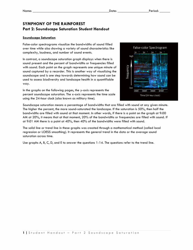
Name: ____________________________________________Date: __________________Period: ______

1 | S t u d e n t H a n d o u t – P a r t 2 S o u n d s c a p e S a t u r a t i o n

SYMPHONY OF THE RAINFOREST Part 2: Soundscape Saturation Student Handout Soundscape Saturation

False-color spectrograms visualize the bandwidths of sound filled over time while also showing a variety of sound characteristics like complexity, loudness, and number of sound events.

In contrast, a soundscape saturation graph displays when there is sound present and the percent of bandwidths or frequencies filled with sound. Each point on the graph represents one unique minute of sound captured by a recorder. This is another way of visualizing the soundscape and is one step towards determining how sound can be used to assess biodiversity and landscape health in a quantifiable way.

In the graphs on the following pages, the y-axis represents the percent soundscape saturation. The x-axis represents the time scale using the 24-hour clock (also known as military time).

Soundscape saturation means a percentage of bandwidths that are filled with sound at any given minute. The higher the percent, the more sound-saturated the landscape. If the saturation is 50%, then half the bandwidths are filled with sound at that moment. In other words, if there is a point on the graph at 9:00 AM at 20%, it means that at that moment, 20% of the bandwidths or frequencies are filled with sound. If at 9:01 AM there is a point at 40%, then 40% of the bandwidths were filled with sound.

The solid line or trend line in these graphs was created through a mathematical method (called local regression or LOESS smoothing). It represents the general trend in the data or the average sound saturation across time.

Use graphs A, B, C, D, and E to answer the questions 1-14. The questions refer to the trend line.

2 | S t u d e n t H a n d o u t – P a r t 2 S o u n d s c a p e S a t u r a t i o n

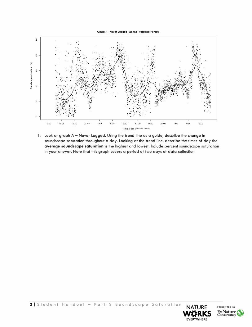
1. Look at graph A – Never Logged. Using the trend line as a guide, describe the change in soundscape saturation throughout a day. Looking at the trend line, describe the times of day the average soundscape saturation is the highest and lowest. Include percent soundscape saturation in your answer. Note that this graph covers a period of two days of data collection.

3 | S t u d e n t H a n d o u t – P a r t 2 S o u n d s c a p e S a t u r a t i o n

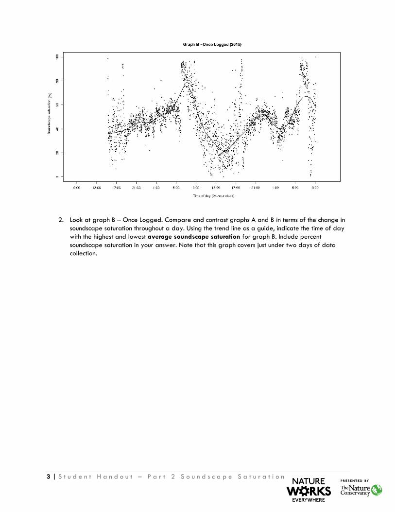
2. Look at graph B – Once Logged. Compare and contrast graphs A and B in terms of the change in soundscape saturation throughout a day. Using the trend line as a guide, indicate the time of day with the highest and lowest average soundscape saturation for graph B. Include percent soundscape saturation in your answer. Note that this graph covers just under two days of data collection.

4 | S t u d e n t H a n d o u t – P a r t 2 S o u n d s c a p e S a t u r a t i o n

3. Look at graph C – Twice logged. Describe the trend in average soundscape saturation in this

graph. What time(s) of day represent peak average soundscape saturation? Describe the overall trend in soundscape saturation for this location. Note that this graph covers a period of two days of data collection.

4. Compare and contrast graphs A, B, and C. What are the major similarities and differences in the average soundscape saturation? Are there any differences in the number of peak periods or the duration of peak periods?

5 | S t u d e n t H a n d o u t – P a r t 2 S o u n d s c a p e S a t u r a t i o n

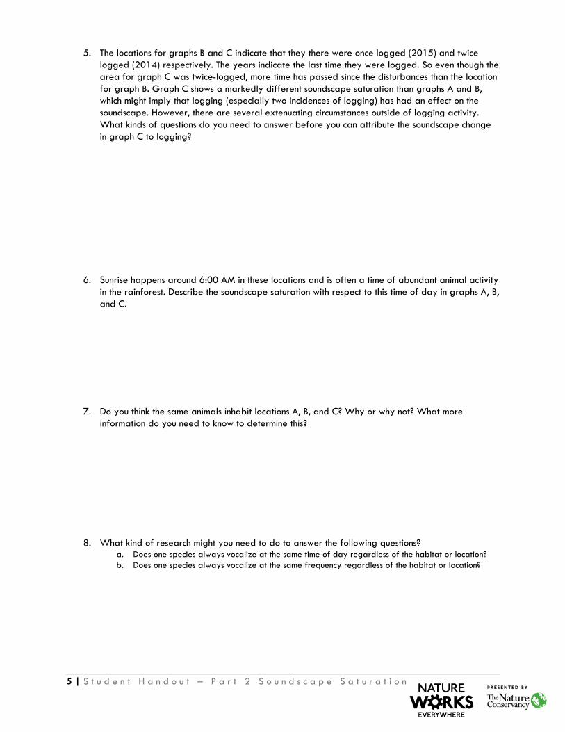
5. The locations for graphs B and C indicate that they there were once logged (2015) and twice logged (2014) respectively. The years indicate the last time they were logged. So even though the area for graph C was twice-logged, more time has passed since the disturbances than the location for graph B. Graph C shows a markedly different soundscape saturation than graphs A and B, which might imply that logging (especially two incidences of logging) has had an effect on the soundscape. However, there are several extenuating circumstances outside of logging activity. What kinds of questions do you need to answer before you can attribute the soundscape change in graph C to logging?

6. Sunrise happens around 6:00 AM in these locations and is often a time of abundant animal activity in the rainforest. Describe the soundscape saturation with respect to this time of day in graphs A, B, and C.

7. Do you think the same animals inhabit locations A, B, and C? Why or why not? What more information do you need to know to determine this?

8. What kind of research might you need to do to answer the following questions? a. Does one species always vocalize at the same time of day regardless of the habitat or location? b. Does one species always vocalize at the same frequency regardless of the habitat or location?

6 | S t u d e n t H a n d o u t – P a r t 2 S o u n d s c a p e S a t u r a t i o n

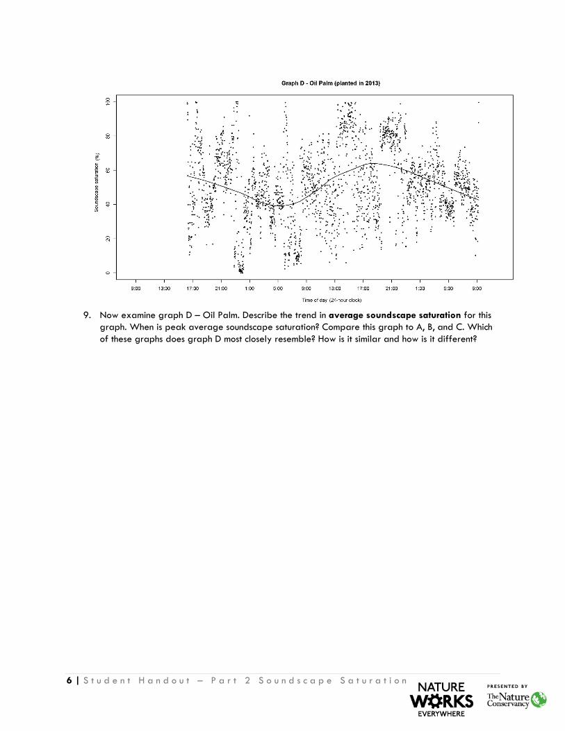
9. Now examine graph D – Oil Palm. Describe the trend in average soundscape saturation for this graph. When is peak average soundscape saturation? Compare this graph to A, B, and C. Which of these graphs does graph D most closely resemble? How is it similar and how is it different?

7 | S t u d e n t H a n d o u t – P a r t 2 S o u n d s c a p e S a t u r a t i o n

10. Based on your examination of graphs A, B, C, and D what conclusions can you draw about

landscape type and sound saturation?

11. As stated in the story map, Bernie Krause introduced the concept of an acoustic niche. This states that every animal species occupies its own acoustic niche in a soundscape to avoid competition for sound space with other species. This hypothesis supports the idea that the healthier and more biodiverse an ecosystem is, the fuller the soundscape will be. Based on this idea, can you assess the relative health or comparative level of biodiversity of the landscapes represented in graphs A, B, C, and D or you need more information than soundscape saturation to determine ecosystem health? If so, what can you determine with the soundscape saturation graphs and what can’t you determine?

8 | S t u d e n t H a n d o u t – P a r t 2 S o u n d s c a p e S a t u r a t i o n

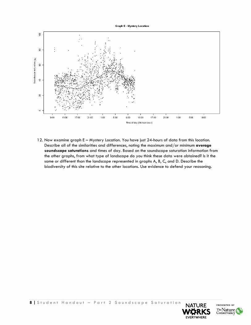
12. Now examine graph E – Mystery Location. You have just 24-hours of data from this location. Describe all of the similarities and differences, noting the maximum and/or minimum average soundscape saturations and times of day. Based on the soundscape saturation information from the other graphs, from what type of landscape do you think these data were obtained? Is it the same or different than the landscape represented in graphs A, B, C, and D. Describe the biodiversity of this site relative to the other locations. Use evidence to defend your reasoning.

9 | S t u d e n t H a n d o u t – P a r t 2 S o u n d s c a p e S a t u r a t i o n

Applications of Acoustic Data

13. If you ran an ecotourism outfit and wanted to make sure you took tourists to the rainforest to see birds and other animals, when would you arrange your tours? How could you use acoustic data to determine this?

14. In what are other ways do you think acoustic data could be useful?

Study Limitations and Experimental Design Choices

15. Does acoustic data capture all of the organisms in an ecosystem?

16. For this acoustic survey in Borneo, the acoustic recorders were strapped to trees at chest height. Describe the advantages and disadvantages of this experimental design.

17. In this particular study, due to time limitations, the number of recorders available, and the number of sites visited, recorders where only placed on trees for 1-2 days at a time. How could this impact the data that was collected and how would you solve for that impact in future investigations?

10 | S t u d e n t H a n d o u t – P a r t 2 S o u n d s c a p e S a t u r a t i o n

18. Ultimately, when designing an experiment, scientists must balance cost and feasibility with their investigation objectives. Time, money, weather, equipment cost, and access (getting permission from logging companies, communities, government, etc. to do research on location) are all factors that must be addressed in experimental design. In a remote forest setting, scientists must even consider how they get to the locations, where they will sleep, and how they will eat and have access to clean water. Even battery life is a concern when using high-tech equipment in a remote location. Because of these factors, scientists must make careful decisions in order to get the most out of their investigations. If you were part of a team who was invited back to the rainforests of Borneo to continue to investigate biodiversity as it relates to land management – what would you like to investigate and how would your investigation compliment the acoustic survey described in this lesson? Describe any limitations or possible barriers to your proposal that you would have to overcome.

11 | S t u d e n t H a n d o u t – P a r t 2 S o u n d s c a p e S a t u r a t i o n

From Biodiversity Study to Land Management

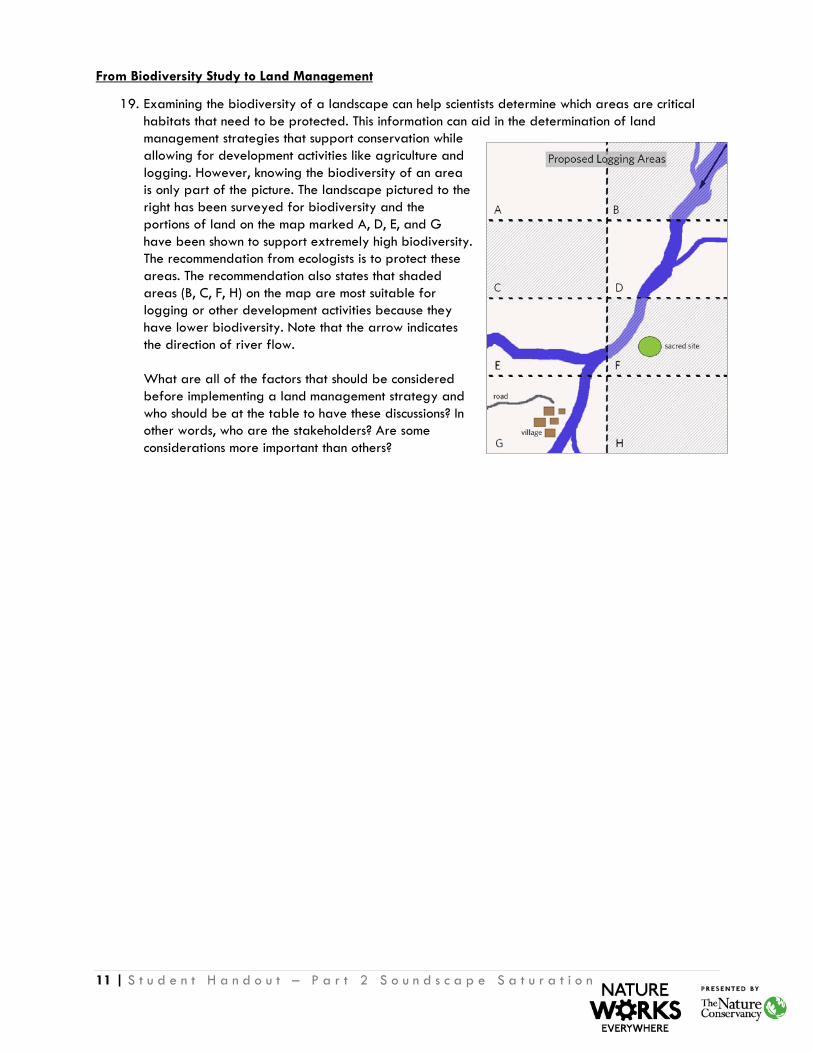
19. Examining the biodiversity of a landscape can help scientists determine which areas are critical habitats that need to be protected. This information can aid in the determination of land management strategies that support conservation while allowing for development activities like agriculture and logging. However, knowing the biodiversity of an area is only part of the picture. The landscape pictured to the right has been surveyed for biodiversity and the portions of land on the map marked A, D, E, and G have been shown to support extremely high biodiversity. The recommendation from ecologists is to protect these areas. The recommendation also states that shaded areas (B, C, F, H) on the map are most suitable for logging or other development activities because they have lower biodiversity. Note that the arrow indicates the direction of river flow. What are all of the factors that should be considered before implementing a land management strategy and who should be at the table to have these discussions? In other words, who are the stakeholders? Are some considerations more important than others?