Symmetry of free-surface flows

Arch. Rational Mech. Anal. 118 (1992) 1-36. �9 Springer-Verlag 1992

Symmetry of Free-Surface Flows

WALTER CRAIG • PETER STERNBERG

Communicated by C. DAFERMOS

Abstract

Certain geometrical properties of steady two-dimensional potential flows in the presence of gravity are considered. The two main problems are that of a solitary wave in an interface between two immiscible fluids of different densities, and that of steady waves in a free surface of a fluid flowing past an object (such as a ship hull, hydrofoil or surfboard). Our results include statements of positivity (or negativity), monotonicity, symmetry and the asymptotic behavior at infinity of such flows. The methods are extensions of those presented in earlier work on the solitary wave [7].

w O. Introduction

In this paper we discuss certain a priori geometric properties of steady potential flows with free surfaces. The problems that we consider are of two- dimensional fluids with gravity, in infinite horizontal configurations that are asymptotic to uniform flow at infinity. We have results for two different problems: (i) surface waves, and (ii) interfacial waves between immiscible fluids of different densities. The surface waves that we consider are steady free-surface flows about solid objects which occupy a finite portion of the top surface of the fluid; these may be envisioned as ship hulls, hydrofoils or surfboards in a flow which is asymptotically uniform. Our results are extensions of work on the solitary wave [7]. The majority of our results apply to flows whose asymptotic velocity is supercritical.

The basic analytic tools of this work are comparison principles for solutions of elliptic partial differential equations. These techniques are well known in the study of free-boundary problems; GISBaRG [10], for example, contains a collection of classical results. In KEADY & PRITCHARD [11] and CRAIG STERNBERG [7] there are new applications to the solitary wave, a free-surface problem in which gravity is present. The results of this paper come from extensions of the techniques of the last reference to the above more complicated settings.

2 W. CRAIG r P. STERNBERG

Our results concerning flows of type (i) consist in giving constraints on the geometry of the flow which are dependent upon the object in the free surface around which the fluid moves. The flow is described by a harmonic velocity potential (0(x, y) ; the top of the fluid is assumed to be given by the graph [(x, y) ; y = F(x)] , which is asymptotic to the x-axis as x ~ • The bot tom of the fluid region, taken to be flat, with depth h is [(x, y) ; y = - h i . The object in the surface of the fluid is represented by a bounded set A c__ R such that for x E A the fluid surface lies at a prescribed height, that is, F(x) is a prescribed function on A. Otherwise, for x ~ R - A, free-boundary conditions are prescribed. The flow is assumed to be uniform at x ~ 4-oo, with velocity c. A flow of this type is called supercritical if c 2 > gh, where g is the constant acceleration of gravity.

Our first results are that if c 2 > gh, and F(x) > 0 for x~A, then the surface satisfies F(x) > 0 for all x ~ R. This is the configuration of a surfboard or planin~ object in a steady flow. The result is proved by a comparison argument, and appears as Lemma 1.2. The analog of the result for the case F(x) < 0 for some x E A is not as definitive a statement, for flows about a ship hull or hydrofoil could change sign, even if they do not do so on the set A itself. Our result is that if c 2 > gh, the global minimum of the surface of a smooth flow cannot occur at a point on the free surface, but must occur on the interior of A. For certain geometries and orientations of objects, as exhibited in Figure 2, the position of the global minimum of a smooth flow is forced to lie on the free surface, and we conclude that any supercritical flows must then contain singularities. Such singularities have consequences in terms of hydrodynamical drag and of forces exerted on the object, and therefore this may have implications in the design of supercritical hulls.

Informat ion about the monotonici ty of supercritical flows is available in the cases where either F(x) > 0 for x ( A , or where it is additionally assumed that the entire surface satisfies F(x )<0 , -oo < x < +oo. The precise statements and conditions for these results are presented as Lemmas 2.2 and 3.1, in the positive and negative cases respectively. Furthermore, if the object in the surface is symmetric and monotone, lying in symmetric position, it is shown that the flow pattern about the object is also symmetric; this is the conclusion of Theorems 2.3 and 3.2. For objects which are at least partially below mean level (F(x)< 0 for some x EA), for which the free surface changes sign, we have only partial results. For numerical results on related problems, see VANDEN-BROECK & KELLER [15] and VANDEN-BROECK [16].

The next set of results concerns internal solitary waves in an interface between two immiscible fluids of different densities. The total fluid depth is taken to be finite, with the denser fluid on the bot tom. We assume that the interface is a graph, {(x, y) ; y = F(x)] . Denote the upper and lower fluid densities by Pl, P2 respectively, and their asymptotic depths as x - o 4-00 by hi, h 2. Steady wave motion of the interface is termed supercritical if c 2 > c~, where

C~= (P 2 - -P l ) g (p~/h~ + pi/h2)

Symmetry of Free-Surface Flows 3

Our first result, appearing as Lemma 1.5 below, is that for all supercritical flows which are not identically uniform, the interface elevation F ( x ) has a given sign, determined by the sign of the quantity

P2 Pl

Along with this, further a priori estimates as to the height and velocity of such interfacial waves are described. One corollary of Lemma 1.5 is that if pz/h 2 = pl/h~, then no supercritical solitary waves exist.

These positivity (or negativity) results are used in w 4 to show that all interfacial solitary waves are symmetric, and monotone on either side of a unique critical point. The proof uses the Alexandrov method of moving planes. For this, it is important to have specific knowledge of the asymptotics of the flow as x ---, 4-w, which is discussed in general form in w 5. The result is the analog of the monotonicity and symmetry of the solitary wave of FRIEDRICHS & HYERS [81, which was proved in [71.

Numerical studies of MEIRON & SAFFMAN [13] have indicated the existence of interfacial waves that are not given as graphs; we do not at present have results on such flow geometries.

In the above results, especially those concerning the monotonicity and symmetry of flows, the asymptotic description of the fluid motion at x ~ 4-~ is important. w 5 is devoted to general asymptotic results about nonlinear partial differential equations in domains consisting of strips; these have a close resem- blance to results of [7] and of B~RESTYCK~ & NIRENBERG [4]. The asymptotic description of solutions consists of two basic statements. First it is shown that any solution in a strip which goes to zero with two derivatives as x---, • for which a parameter value corresponds to supercritical velocities, does so at an exponential rate. Supercritical parameter values are those for which zero does not lie in the continuous spectrum of the linearized free-boundary conditions. This decay result is a version of a nonlinear Lindel0f principle for solutions of partial differential equations in strips.

Secondly, an asymptotic expansion of solutions as x ~ 4-oo is shown to hold; this is in terms of solutions of the linearized problem, and is similar to work of AGMON & NIRENBERC [1] in the linear case. These asymptotic results, along with the positivity (or negativity) results of w 1 are crucial to the monotonicity and symmetry statements of w167 3 and 4.

The basic technique used in the above work is the Maximum Principle for harmonic functions, and several related comparison principles. For completeness, statements of these principles are given here; the versions are sufficient for our needs, but are by no means the strongest statements that can be made. The first comparison principle concerns the boundary behavior of a positive harmonic function at a point at which the boundary is smooth.

Lemma 0.1. (The Hopf Lemma). Let S c= R 2 be a domain in which a noncon- stant function ~P(x, y) ~ Ca(S) satisfies

A ~ = 0 ,

~>_0 .

4 W. CRAIG • P. STERNBERG

I f ( ~, rl) ~ OS is a boundary point at which the boundary has a well-defined tangent line, and if T ( ( , ~l ) = O, then

ON}[J(~, FI) < 0

for N the exterior normal vector at (~, I'/) to OS.

This lemma is used throughout this paper: in the results of a priori positivity (or negativity), in estimates of the amplitude of the free surface flow and its velocity, and in the proofs of monotonicity of solutions. In order to demonstrate symmetry of solutions, the Alexandrov method of moving planes is used. In our setting, further knowledge of the behavior of positive harmonic functions in corners of a domain is needed. Sufficient information is supplied in this second comparison result.

Lemma 0.2. (The Hopf 'Corner-Point' I_emma). Consider S c= R 2 and T(x, y) ~ CI(s) as above, and let ((, t?) ~ OS be a boundary point at which the boundary curve is not smooth, but consists o f two C 1 arcs meeting with an interior angle ~ >= ~. (That is, interior tangent vectors tl, t2 to the two arcs have t 1 �9 t 2 <_ 0). Let v = atl + bt2 for some a, b > 0; the vector v points into S. I f T(( , ~/) = 0, then either

(i) O~,T(~, ~) > 0

or else

= = o W ( ~ , ~ ) > o . (ii) OvT(~, 17) 0 for all such v, t l . t2 0 and 2

We refer to [9] for more general statements of these two results, and their proofs.

In noncompact domains, some control on the asymptotic behavior of solutions at infinity is needed in order to start the method of moving planes. In the present work, sufficient control is given through a rigorous asymptotic expansion of solutions of an appropriate nonlinear elliptic partial differential equation. It turns out that this asymptotic description of solutions is a very general fact about nonlinear elliptic problems in strips, and the exponential asymptotic behavior is related to certain LindelOf principles for linear partial differential equations. These results are presented in compact form in w 5.

w 1. Comparison Results

The mathematical formulations of the various fluid dynamical problems that are considered in this paper are conveniently given in terms of the velocity potential and stream function as independent variables. Using these formulations, we shall describe several a priori results on the possible configuration of the free surface. These results are obtained by using the Maximum Principle and the Hopf Lemma on the boundary behavior of harmonic functions. Among the conclusions are several results on the nonexistence of a smooth


steady flow about certain geometries of objects in the fluid surface. The two general classes of problems that are discussed in this paper are (1) free-surface problems with gravity, with objects (such as ship hulls, planing surfaces or hydrofoils) in the surface, and (2) steady gravity waves in an interface between two immiscible fluids in a fixed region of infinite horizontal extent. In this section, the formulations of problems (1) and (2) are given, and the comparison results are derived.

Free surface problems with objects in the surface. The first problem concerns a two-dimensional fluid with a free surface under the influence of gravity. An impermeable solid object of given geometry is taken to lie within the top surface of the fluid; the corresponding boundary value problem is of mixed type. The surface of the fluid region consists of two sets, the region in contact with the solid object, and the region in which the surface is free, on which the fluid must satisfy the Bernoulli condition. In physical variables the fluid region is taken to be [(x, y) ; - c o < x < +0% - h < y < F(x)}. The upper fluid boundary (x, F(x)) and the velocity potential q~(x, y) which describes this steady flow satisfy:

0nq ~ = 0 for all (x, F(x)) on the upper fluid boundary,

F(x) is prescribed by the solid object on the fixed port ion of the upper fluid boundary,

c 2 (1.1) ~ ( V ~ ) 2 -[- gF= -- for (x, F(x)) on the free port ion of the

2 upper fluid boundary,

s for - c~ < x < +c~, - h < y < F ( x ) ,

0nq~ = 0 for y = - h .

This paper addresses principally the problem of flows which are localized per- turbations of a uniform flow; that is, we take as asymptotic conditions as x---~ 4-00

(1.2) @(x, y) ~ - cx , Vq~(x, y) ~ ( - c , 0).

y

f f A

X

-h A

Fig. 1. The solid object, given by the arc AB, embedded in the free surface of the solitary wave.

6 W. CRAIG ~L P. STERNBERG

The partial differential equations (1.1), (1.2) are equivalent to a nonlinear problem for the conformal mapping of a fixed region into the fluid region. This is often called a 'hodograph transformation', whose independent variables are the velocity potential q~ and the stream function ~ for (1.1).

It is more convenient to introduce variables (~, ~ ) = (l/c)(q~, ~) in the region S={(~ , r / ) ; -oo < ~ < +0% - h < r / < 0 } . The conformal map is Z(~, r l )= ( X + iY) (~ , rl), which by the asymptotic conditions (1.2) satisfies ( X , Y ) ~ (~,t/) as I~ [~~176 Denote X(~,r l ) = ~ + x ( ~ , t l ) , Y(~,rl) = 1/+ y(~, q), where (x + iy) (~, Jl) is the perturbation of the conformal map from the one for a uniform flow. Under this transformation the top boundary 0 = {(~, 0), -oo < ~ < +co} of S is transformed into the upper fluid boundary of the fluid region, and thus 0 is divided into two sets. One is the preimage of the free surface, which we denote by 01; the remaining region 02 is the preimage of the boundary of the contact between the fluid and the object in the surface. The set 01 is taken to be closed, and 02 to be bounded. In these coordinates the problem is most conveniently posed for the function y(~, r/) in the region S:

(i 3) 2g

1 + c ~ (Or 2 + (1 + O~y) 2

y(~, o) = r ( x ( r o))

A y = O

y(~, - h ) = 0

The asymptotic condition is that

y = 1 for t /= O, ~ 0 t (the free boundary),

for ~ = 0, ~ E 02 (the fixed boundary),

for (4, t/) ~ S,

(boundary conditions on the bottom).

(1.4) (y, 0r O,y) ~ 0 as ~ ~ •

In Section 5 we shall obtain a priori decay estimates for supercritical flows which will quantify this decay property.

To ensure the existence of the hodograph variables described in the preceding paragraph, and the equivalence of (1.1), (1.2) to (1.3), (1.4), we refer to [7] in which the following lemma is proved:

Lemmal.1. Given a C 1 solution to (1.1), (1.2) in the fluid region - ~ < x < + ~ , - h < y < F(x ) , the transformation Z(~, rl) exists and is invert- ible, and the variables (~, r/) = (i/c) (~, gt) are global variables defined over S. Furthermore, if no physical evacuation of the channel occurs, that is, i f Y(~,O) > - h , then O,y(~, t l ) > - 1 for all (~, t l ) ES.

Several comparison results are derived easily from formulation (1.3). The first is the observation that 1/I VYI2> 0; thus, for any G0 ~ 01, the boundary conditions imply that

C 2 0.5) y(~o, o) < - - .

2g


This is a simple upper bound on the height attainable by a point on the free surface. If equality occurs in (1.5), the surface must possess a singularity, analogous to the Stokes wave of extremal form. In other settings, this estimate is well known [11, 14].

A second result consists in a bound from below for the highest crest or lowest trough of a wave, if it occurs on the free surface. Consider first the highest crest. Assume that max~eRy(~, 0 )=Y(~0 , 0 ) > 0 is a positive crest which is attained at a point ~0~ 01 on the free boundary. A comparison

y(~0, 0) solution for this is the uniform flow given by l(~, r / ) - ( r / + h),

h since clearly l ( ( , 0) >__y(~, 0), l ( ( , - h ) = y ( ~ , - h ) = 0 and l ( ( , t/) > y(~ , r / ) ~ 0 as (--~ 4-oo. The Strong Maximum Principle implies that l ( ( , 17) > y(~, t/) for all (( , r/) ~ S. One uses the Hopf Lemma to compare the normal derivatives of l and y at ((0, 0):

(1.6)

O~y(~o, O) > O~l(~o, O) =

O~y(~, O) = O.

y(~o, 0) h

Since ~0 E 01, this strict inequality is used in the Bernoulli condition

1 2g 1 2ghm C 2 Y (1 + m) 2 c 2 ' (1.7) 1 = (1 + Oqy) 2 + (0r 2 + - - < +

where Y(~0, O)/h=--m >_ 0 is used. This is a constraint on m, which, for m =r 0, can be rewritten as

(1.8) m 2 + ( 2 - 1 F 2) m + ( 1 - F 2) > 0

for F 2 = c2/gh, the square of the Froude number. Let m+(c) denote the rightmost root of the quadratic (1.8); it follows that m > m+(c). For c 2 __> gh, that is, for F__> 1, the root m+(c) >= O. This gives a lower bound on the maximum amplitude of a solution if it is attained on the free surface. This is also expressed as F 2 < 2 ( m + 1 ) 2 / ( m + 2 ) , which has appeared in [14] in a discussion of the solitary wave.

The next consideration is for the lowest trough of a solution of (1.3). Assume that min~eRy({, 0 ) = Y({0, 0 ) < 0, the lowest trough being attained at ~0 ~ 01 on the free surface. The analogous comparison solution is l({, r/) =

y(~o, o) - - ( t / + h), which by the Maximum Principle satisfies l(~, t/) < y(~, t/)

h for all (~, r/) ~ S. The same use of the Hopf Lemma gives the comparison of derivatives at (~0, 0) :

Y(~0, 0) O,y(~o, O) < O~l(~o, O) - < O,

(1.9) h Ocy(~o, O) = O.

8 W. CRAIG • P, STERNBERG

We are assuming that the minimum trough is attained on the free boundary; hence the Bernoulli condition implies

2g 1 1 (1.10) 1

--c2 y(~0, 0) = (1 + Ony) 2 + (O~y) 2 > (1 + m ) 2

where now Y(~0, O)/h=--m< O. We have used the fact that O~y(C, r l )> - 1 , which is derived in Lemma 1.1. Thus the minimum value m satisfies the inequality

2gh 1 1 c S - m > (1 + m)2 ,

which for m < 0 is equivalent to (1.8). We learn that m > m+(c). Since m+(c) >_ 0 for c2__> gh (F>_ 1) this is incompatible for the free surface of a supercritical flow. We have proved

Lemma 1.2. Consider smooth flows Y(C, rl) ~ CI(S) that satisfy (1.3). (1) Assume that the highest crest max~el~y(C, 0 ) > 0, which is attained at a point of the free surface ~o~ 01. Then the amplitude is bounded from below:

hm+(e) < Y(Co, 0).

This is a non-vacuous estimate for c2>= gh. (2) Assume that the minimum trough min(eRy(C , 0) < 0, which is attained at a point of the free surface ~o ~ 01. Then the minimum amplitude is bounded from below by the same constant:

hm+(c) < Y(Co, 0).

Using this 1emma we can draw conclusions about the flow configuration based solely on the geometry of the object in the surface. The first result is the positivity of free surfaces, given objects which lie entirely above the asymptotic limits of the fluid. If there is no object, so that the upper fluid boundary is entirely a free surface, the conclusion is that all supercritical solitary waves are positive, which recovers results of [7].

Corollary 1.3. Assume that y ( C, rl ) ~ C 1 ( ~) gives a smooth flow, with C 2 ~ gh. I f the object is entirely elevated above the asymptotic limits of the fluid, that is, if F (X(C,O) ) > 0 , C~02, then y(C,O) >O for all - ~ < C < +co.

The second conclusion is about the possible configuration of a supercritical flow which has portions of the upper fluid boundary lying below the asymptotic limits of the fluid.

Corollary 1.4. Assume that y (C, ~l) ~ C l (~) is a smooth supercritical flow. Sup- pose that ~o is a negative global minimum of the upper fluid boundary: y (Co, O) = minr Y(C, 0) < 0. Then Co must lie in the interior of a2, that is, any negative minimum fluid level must occur on the solid object, and cannot occur on its edge.


ND~\ . / H

a -h

X

b -h i

P

X

Fig. 2. (a) A planing object or hull (double line) with its minimum occurring at its left endpoint (below A). The dashed curve CDE represents a free surface for a smooth flow which is precluded since the minimum does not occur in the interior of the object. The solid curve FGH represents a free surface for a possible flow which necessarily possesses a singularity at the left endpoint of the object. (b) A planing object or hull (double line) with a nonunique minimum occuring at the left endpoint. Even in this configuration, the smooth flow CDf~ is precluded. The singular free surface FGH is again a possibility.

Y

h.

Q2

-h 2

t X

Fig. 3. The interfacial solitary wave F separating fluids of densities Pl and &.

10 W. CRAIG • P. STERNBERG

This is a nonexistence result for smooth flee-surface flows for solid objects with certain geometries. In particular, if the specified object profile F(x) , A < x _ B, has its minimum point at either A or B, Corollary 1.4 excludes the possibility of a flow y~ CI(S) (Figure 2a). Even if the minimum point (A, F (A) ) is not a unique minimum (for example Figure 2b), steady supercritical flow cannot be smooth at A, and must contain a boundary singularity. Such singularities have consequences in terms of the forces exerted on the solid object and hydrodynamical drag. In cases of hulls or hydrofoils, geometrical considerations in their design could reduce or eliminate these singularities.

Waves in an interface between two immiscible fluids. A second class of problems addressed in this article concerns waves in a free interface between two horizontally infinite bodies of fluid, again under the influence of gravity. We discuss the two-dimensional problem, assuming that the flow is steady, and is an asymptotically uniform flow as x ~ • co, with the same velocity for each fluid. Equivalently, this describes a wave propagating without change of form in this double layer of fluid which is taken at rest at x--, •

We retain four parameters describing this problem: the asymptotic depths of the fluid layers, h 1 and h2, as x -* 4-00, and the fluid densities p~, P2. The density Pl will refer to the upper fluid density, which will be taken to be less than 192.

In physical variables, the free interface F(x) and the velocity potentials for the upper and lower fluid bodies, r ~2 (x ,y ) , satisfy the following system of equations:

Oyqb 1 = 0

(1.11)

f o r

Oy~2 = 0 for

& ~ba = 0 for

A ~b 2 m 0 f o r

y = h i ,

y = - h a ,

-c~ < x < +r F(x) < y < h l ,

- -oo < X < + c % - h 2 < y < F(x)

pl �89 e + F ( x ) - =p2 ~lVq~2 + F ( x ) -

for y = F(x) (the Bernoulli condition on the interface).

As above we consider sufficiently localized solutions; that is, we impose asymptotic conditions as x--, 4-00:

(1.12) ~j(x, y) --+ - c x , Vq~j(x, y) ~ ( - c , 0), for j = 1, 2.

Our comparison results are most conveniently described in coordinates analogous to the hodograph transformation; that is, one considers the equivalent problem of finding conformal mappings from fixed domains onto the regions occupied by the two fluids. Consider (r Tj), j = 1, 2, the velocity potential and stream function for the two fluid regions, with ~ l ( x , F ( x ) ) = ~ 2 ( x , F ( x ) ) = 0 for normalization. Define two fixed domains, S i = { ( ~ , t / ) : - o ~ 1 7 6 hi} and S 2 = { ( ~ , t / ) : - c ~ <

Symmetry of Free-Surface Flows 1t

< --}-0% - h 2 < / , / < 0}, and set (c~, c~/) = (~1, T1) in $1, (c~, c/']) = (q~2, 5u2) in $2. The problem (1.11), (1.12) is equivalent to a system of differential equations for the conformal maps Z 2 = (Xj + iYj) (~, r/), j = 1, 2, from the fixed domains S1, $2 into the regions occupied by the two fluids. Letting Zj = (~ + xj (~, ~1), rl + yj (~, rl)), we can state the problem in terms of yj(~, r/):

(1.13)

& Y l = 0 in $1,

Yl(~, hi) - -0 , ~E R (boundary conditions for a fixed top),

Ay 2 = 0 in $2,

Y2(~, -h2 ) = 0, ~ ~ R (boundary conditions for a fixed bottom),

(yj(~, ~), Ocy;(~, ~), O, yj(~, r/))--. 0 as ~-* 4-oo

(asymptotic conditions at infinity).

Boundary conditions on the fluid interface from (1.11) correspond to a match- ing condition across the boundary {(~, 0 ) , - o o < ~ < +oo}. Define l(~) through the relation X2(I(~), 0) = XI(~, 0); then

(1.14) Yl(~, 0) = r (Z~(~ , 0)) = F(X2( l (~) , 0)) = y2(I(~) , 0 ) ,

which matches the vertical displacements of the interface. Furthermore, the Bernoulli condition becomes

1 2g ) (1.15) Pl (0~yl) 2 + (1 + 0~yl) 2 -[- c 2 y 1 - 1

1 2g ) l(4) = P2 (04y2) 2 + (1 + 0,7y2) 2 + c 2 Y2 - 1 .

This double 'hodograph transformation' is equivalent to the problem (1.11), (1.12); as in the previous case, Zi and Z2 give global variables to the two fluid regions. Additionally, one finds that if neither fluid layer is breached, so that - h 2 < F ( x ) < F ( x ) < hi, then we have the estimate from below: O,TY:({, 0) > -1 , j = 1, 2.

The hodograph variables are useful in obtaining comparison results similar to Lemma 1.2. The strongest results are obtained for supercritical velocities: c 2 > c0 2, where we define

(1.16) c 2 = (P2 - P l ) g (pl/hl -t- p2/h2)"

The significance of the critical velocity is discussed in Section 5; for c 2 > c0 a, zero is not in the spectrum of the linearizafion of the Bernoulli condition (1.15).

12 W. CRAIG & P. STERNBERG

Lemma 1.5. Assume that yj(~, 11)~ C l ( ~ ) , J = 1, 2, are solutions to (1.13), (1.14), (1.15), giving rise to a smooth steady flow. Let M and m denote possible extremal values of the interface; M = supper yj(~, 0), m = inf~R yj(~, 0). (i) There are upper and lower bounds M+(c) and m+(c) (which are algebraic functions of c > 0 and the parameters Pl, P2, hi, h2) such that

- h 2 <= M_(c) <= M <= M+(c) < hi ,

- h 2 < m_(c) <= m < m+(c) < hi.

I f the extremal value is attained at some finite point ~o for a nontrivial solution, then strict inequality holds. (ii) I f c 2 >= c 2 and (pl /h 2) - (p2/h~) <= O, then m = O, and all C 1 solutions of (1.13), (1.14), (1.15) that are not identically zero must be positive: F (x ) > O. (iii) I f c 2 >= c~ and (pl/h~) - (P2/h~) >= O, then M = 0 and all nontrivial C 1 solutions of (1.13), (1.14), (1.15) are negative: F (x ) < O.

Combining cases (2) and (3) of the above lemma we obtain an interesting nonexistence result.

Corollary 1.6. I f p l /h 2 - p 2 / h 2 = O, then no nontrivial supercritical solutions exist. For any given fluid densities Pl, P2, and fixed total height h = h 1 + h2, there is a unique proportion aft (0, 1) such that for f luid levels hi = ah, h 2 = (1 - a ) h , the above difference vanishes, and thus there exist no nontrivial solutions to (1.13)for any supercritical velocity c2>= c~.

Proof. Suppose that Y(~0, 0) attains a nonnegative maximum at the point ~0; we may assume by translation that ~0 = 0, and also that l (~0)= 0, so that M = sup~RYl(~, 0) = y l ( 0 , 0) =y2(0, 0) >= 0. Then O~yj(O, 0) = 0 for j = 1, 2, and we may compare separately Yl and Y2 with the corresponding uniform flows having the same asymptotic velocities. If the yj(~, tl) are not identically zero, by the Maximum Principle

(1.17)

- M Yl(~, r/) < - - ( r / - hi) in S1,

hi

M Y2(G r/) < ~ (q + h2) in $2.

h2

At the boundary point (~, r/) = (0, 0), the Hopf Lemma gives the inequalities

- M M (1.18) 3~yl < h~-' O~Y2 > h2

Making the physical assumptions that M < hi, we know that 3nyj > - 1 , for j = 1, 2. This information is used in the Bernoulli condition (1.15) to obtain


an inequali ty for M:

(1.19) Pl (h 1 ~ M) 2 + c ~ - 1 < /32 ( h 2 q_ M) 2 q- c ~ - 1 .

We rearrange this inequality, and define

plh2 p2h2 b(s, c ) = (/32 - / 3 1 ) ~ - 1 a(s) - (hi _ s) 2 (h2 - - S ) 2 ,

to conclude that

(1.20) a(M) < b(M, c) for M __> 0.

Considerat ions o f a nonposit ive m i n i m um m achieved at ~0 = 0 are similar; one obtains the inequali ty

(1.21) a(m) > b(m, c) for m =< 0,

for solutions which are not identically zero. The results o f Lemma 1.5 will follow f rom analysis o f the algebraic in-

equalities (1.20) and (1.21). The basic properties o f a(s) and b(s, c) are (i) a'(s) > 0 for - h 2 < s < hi, (ii) a ' ( 0 ) = ash(O, Co) for critical velocity Co defined in (1.16) and (iii) a(s) has only one inflection point in the interval - h 2 < s < h 1. The feasible set for (1.20) and (1.21) are the intervals (M_(c) , M+(c)) and (m_(c ) , m+(c)) respectively, f rom proper ty (iii). I t is clear that if a ' (O) <= O, then m_(c) __> 0, while if a ' ( 0 ) __> 0, the inflection point o f a(m) is nonposit ive and m+(c) <= O. Comput ing a" (O) = 6 ( (pl /h 2) - (p2/h2)), we establish statements (2) and (3) o f the lemma. []

Amplitude

hi

M§

M_(c)

-h2

D

,-C

Fig. 4. For fixed values of the parameters Pl, P2, hi, and h 2 and for wave speed c, the - - A

segment BE bounds the possible amplitude of the interfacial wave. The arc ABD is the A

graph of M+(c) and the arc DEF is the graph of M ( c ) . The values c o and c I bound all possible wave speeds.


Interesting features of these comparison results are the bounds placed upon the possible supercritical solutions and their velocities. For fixed parameter values Pl, P2, hi, h2 there is a maximum velocity Cl _-> Co at which any nontrivial steady solution can travel. Furthermore, there are bounds from above on the amplitude of supercritical solutions. Finally, we will prove in Section 4 that the required positivity/negativity results of Lemma 1.5(ii),(iii) are starting points for the results on the symmetry of all supercritical interfacial w a v e s .

Solitary waves in fluid dynamics are usually associated with supercritical velocities. However, the bounds of Lemma 1.5 indicate that the presence of upper and lower boundaries of the fluid region require that solutions with larger amplitude slow down. It is natural to ask the question: Do bifurcation branches of solitary wave solutions become subcritical as the amplitude of the solutions increase? In the case p l / h 2 = p2/h 2 no supercritical solutions exist; however, the bifurcation branches may lie entirely within the subcritical region. Certainly subcritical solitary wave solutions would be unstable, if indeed they did mathematically exist. A final question concerns the possibility of an analog to the Stokes wave of extremal form. Lemma 1.5 implies that without c = 0, the singularity of F ( x ) is required to lie within the fluid region itself, on the boundary between two fluids. At this hypothetical singularity, one fluid velocity would tend to zero, while the other would become infinite - a situa- tion which we find implausible. We conjecture that the analog of a singular wave of extremal form does not exist for this problem. The global bifurcation problem for this setting remains to be fully worked out.

w 2. Planing Objects above Mean Level

We focus here on the properties of solutions of (1.3) in which a planing object lies above mean level; that is, we assume that

(2.1) y ( ( , 0) = F ( X ( ( , 0)) > 0 for {e02.

By Lemma 1.1, this immediately implies the positivity of y(~, 0) for all ~, since an absolute minimum cannot lie on the free surface.

We first describe the asymptotic behavior of a solution of (1.3).

Lemma 2.1. Suppose n > 2 and some O< asymptotic estimates:

c 2 > gh and y~ CI+~(S) n cn+a(S\02) for an integer cz <= 1. I f y satisfies (1.3), then it satisfies the following

ll 12 O~O~(y(~,Jl) - r l e - 7 ~ sin y l (~ /+ h))J < e -s~ as ~ oo,

for all (ll, 12) such that l 1 + l 2 <= n - J, for some rl > 0, and for any s such that Yl < s < rain (2y 1, Y2). The decay rate Yl and the value Y2 are determined from linear theory; 71 is the smallest positive root o f cot(Th) = c2/g7, and Y2 is the next smallest root. A similar decay estimate holds as ~ ~ -oo.


The proof follows from Lemma 5.11 on noting that equations (1.3) take the form of (5.5). We now give a sharper characterization of the regions of monotonicity for a solution y of (1.3).

Lemma 2.2. Let y be a C 1 (S ) solution of (1.3) for c 2 > gh satisfying condition (2.1). There exist vertical lines {( =2r} and {( =An}, 2L_- < An, such that Ocy((, 7) > 0 for ~ < 2~ and 7 ~ ( -h , 0), while O~y(~, 7) < 0 for ~ > 2~ and 7~ ( -h , 0). Furthermore, strict monotonicity also holds on the free surface; Ocy(~, O) > 0 for ~ ~ (-0% 2~) n O~ and Ocy(~, O) < 0 for ~ E (An, ~ ) n 0~.

Proof. We first introduce some notation. For any 2, ( e R, let ~ = 2 2 - be the reflection of ( with respect to 2, and define the reflected function Yx((, 7) =Y((;~, 7). Denote w ;~ =y~ - y and v x =y~ +y . Then let L x be the half strip {((, r/) : ( < 2, - h < 7 < 0} and R; = {((, 7) : ( > 2, - h < 7 < 0}. Now define

(2.2) 2L = sup {2 :wi(~, I?) > 0 for all (~, 7) in L ~, 2 < 21,

(2.3) 2R = inf {2 :w~(~, 7) > 0 for all (~, 7) in R ~, }L > 2/.

LEWY [12] has shown that a C 1 solution of (1.3) is actually real-analytic on S\02, so the asymptotic results described in Lemma 2.1 apply. These estimates imply that w;'(~, 7) > 0 for (~, 7) in L ; and R z when 2 is respectively sufficiently negative and positive. Hence -oo < 2 L __< 2R < cr For any 2 E R, w ;~ (~, 7) satisfies

Aw ;~ = 0 in S,

w~(2, 7) = 0 for - h ____ 7 _-< 0, (2.4)

w)~(~, - h ) = 0,

l i m w x(~ ,7) = 0 . Ir

Furthermore, if one denotes 0/~ = [~ : ~x E Oi} for i -- 1, 2, then (1.3) yields the following top boundary condition for wX(~, 0):

(2.5) ( 2 ; - Y ; ) ( 2 + O ~ v ~ ) O " w ~ + 0r ( ; ; -Y~ ) OCw;~

-(O~y-t- (1-t-Ony)2)wX=O for 7 = 0 and ~E01(30 ~.

By (2.2), wX(~, 7 ) > 0 for ~ < 2 < 2 L a n d - h < 7 < 0 , while wX(2, 7 ) = 0 . The Hopf Boundary Point Lemma applied to w )~ along the segment (2, 7) for - h < 7 < 0 then gives

(2.6) 0r 7) = _1 0r 7) > 0 for (2, 7) ~L ~L.

A similar argument yields the analogous result for (r 7 ) ( R zR.


To prove the last statement of the lemma, note that for 2 ~ ( -co , 2L) n 01,

(2.7) W 2 O~lw ~. 2 2 = =O~w = - O ~ w ~ = 0 at ( 2 , 0 ) .

Furthermore, (2.6) gives O~wX()L, 0)__< 0. If, however, O~w~(2, 0 ) = 0, then differentiating (2.5) with respect to ~ and using (2.7) yields

(2.8) (y ;;) - ( 1 + O~y) Onw~(2, O) = O.

In light of Lemma 1.1 and (1.5), this would imply that O,O~wX(2, 0) = 0, and w ~ would be a positive harmonic function in L z which vanished to second order at the corner point (2, 0). This violates Lemma 0.2, and we conclude that O~y(2, O) = _10~w~(2, 0) > 0 for 2 E ( -0% 2L) C~ 01. A similar argument applies to prove the analogous result for 2 E ()LR, Oo) n 01- []

It is natural can be given if interesting class monotone in the

to expect that a clearer description of the solution to (1.3) more information is specified about the planing object. An of objects to study consists of those objects which are following sense:

Definition. F(x) is monotone if there exists a point (x0, F(xo)) on the object such that if (x, F(x) ) is any other point on the object, then F ' (x) __< 0 for x > x 0, while F ' (x)__>0 for x < x 0.

If the above inequalities are strict, we shall call the object strictly monotone. Specializing further, one might consider symmetric, monotone objects, that is, monotone objects which also satisfy F(x) = F ( 2 x 0 - x).

Theorem 2.3. Let y be a C 1 (S) solution of (1.3) with C 2 > gh and F(x) > O. (i) If the object is monotone and its minimum occurs at A = X(a, 0), then 2 L given by (2.2) satisfies 2L > a. I f y(a, O) = y(b, O) where B = X(b, 0), then a < 2L <- )~R < b. (ii) If the object is either strictly monotone and symmetric about x o, or

a + b F(X(~ , 0)) is constant for ~ ~ 02, then y(~, rl) is symmetric about ~ - and monotone to either side of the center. 2

The results of Lemma 2.2 and Theorem 2.3, part (i) can be viewed as defin- ing a partition of the fluid region into three subregions: f2 L, DR and s the boundaries between these three sets are the images of the curves (2L, r/) and (2R, ~/) for - h __< ~ __< 0 under the conformal map Z (see Figure 2.1). Recall that q~ = c~ so that images of vertical segments in the (~, q)-plane are level lines of the velocity potential. Also

1 l( x det (VZ) O~y 1 + O , y / c 09y q/y


where det (dZ) = (1 +Orly) 2 + (0~y) 2 >0, hence (fly -~- c3r (dZ). Since Sr-~ L and DR are respectively the images of L )~L and R xR under Z, and since 3~y > 0 in ~2 L, 3~y < 0 in E2 n, the highest point on each streamline lies in [20. In case the object is symmetric, then (ii) says that f20 is the vertical line {(,~R, , ) ; - h __<, = 01.

A B

-h

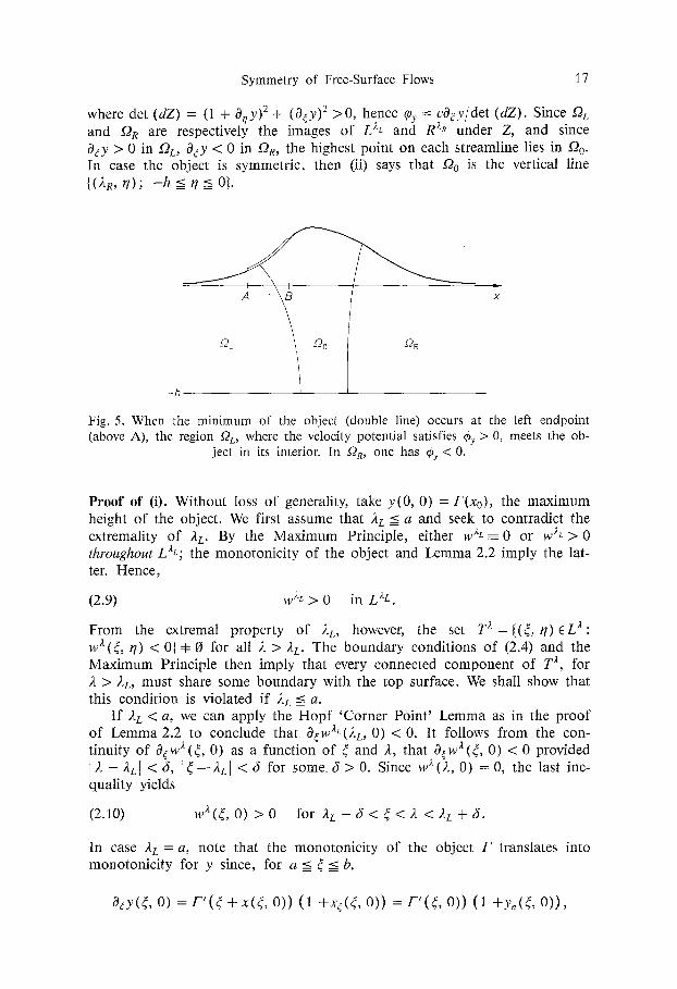
Fig. 5. When the minimum of the object (double line) occurs at the left endpoint (above A), the region OL, where the velocity potential satisfies 0y > 0, meets the ob-

ject in its interior. In De, one has 0y < 0.

Proof of (i). Without loss of generality, take y(0, 0) = F(xo), the maximum height of the object. We first assume that 2 L ___< a and seek to contradict the extremality of 2L- By the Maximum Principle, either w & ~-0 or w& > 0 throughout L&; the monotonicity of the object and Lemma 2.2 imply the latter. Hence,

(2.9) w & > 0 in L ~L.

From the extremal property of 2L, however, the set T ~ ={(3, r / )EL~: wX(~, r/) < 0 1 . 0 for all 2 > 2L. The boundary conditions of (2.4) and the Maximum Principle then imply that every connected component of T ~, for 2 > 2L, must share some boundary with the top surface. We shall show that this condition is violated if Z L _ a.

If 2L < a, we can apply the Hopf 'Corner Point ' Lemma as in the proof of Lemma 2.2 to conclude that 3r 0) < 0. It follows from the continuity of O~w~(~, 0) as a function of ~ and 2, that O~w~(~, 0) < 0 provided ] 2 - - ~ L [ < g, 1~--2L[ < g for some g > 0. Since wX(2, 0) = 0, the last inequality yields

(2.10) w;~((,O) > 0 for 2 L - - g < ~ < ~ < 2 L q - g .

In case •L = a, note that the monotonicity of the object F translates into monotonicity for y since, for a _-< ~ __< b,

Ocy(g, O) = F ' ( 4 + x ( G 0)) (1 +xr 0)) = F ' ( ~ , 0)) (1 +Yn(~, 0 ) ) ,


and 1 + y , ( ( , 0 ) > 0 from Lemma 1.1. Thus O(y(~,O) =>0 for a_<_(__<0, and since Or 0) > 0 for ~ < 2L = a, one has, for some ~ > 0,

w~(~, 0) _> 0 for a - O < ( < 2 < a + ~ .

Therefore in either the case 2L < a or 2L = a, any component of T ~ must share boundary with the top surface away from a 0-neighborhood of the corner (2, 0) for 2 < 2L + ~.

Next consider the asymptotic behavior of wX((, t/) as ( ~ -oo. From the asymptotic description of y( ( , r/) given in Lemma 1.1, wX((, 0) = yX((, 0) - y(~, 0) - r (2) e ~1r By (2.9), w ~ > 0 so r(2L) > 0. Hence there is a ~1 > 0 such that r ( 2 ) > 0 for 2 < 2~ + ~1. This implies that for such 2, T ~ stays within a bounded set, outside of which w;~> O.

Finally, we rule out the possibility that there exists a 40 < 2~ satisfying w~((0, 0) = 0. If (0 ~ 0a c~ 0(% then Ocw~((o, 0) = 0; however, this violates the Hopf Lemma since O~w;~(~o, 0 ) = 0 in light of (2.5). If (0~0x n02 z~, then for some small e > 0, one would have

0 = y ~ z ( ~ 0 , 0 ) - Y ( ~ o , 0 ) > y ( a + e , 0 ) - y ( ( a + e ) ~, 0) = wZ~((a + e) ~, 0),

using Lemma 2.2 and the minimality of y(a, 0) on the object. Since 2L --< a, it follows that (a + e) ~ < 2L, and the last inequality violates the positivity of w ~z in L ~z. We conclude that

(2.11) w~(~, 0) > 0 for ~ < 2L.

The contradiction is reached, for T ~ cannot share any boundary with the top surface for 2 - 2L sufficiently small.

If y(a, O) = y(b, 0), then the result 2~ < b can be proved similarly.

Proof of (ii). Again take y(0, 0 )=-F(xo) . We show that 2 L = 0--2R, to deduce symmetry. Assume that 2 L < 0; as in the proof of (i), we seek to contradict the criticality of 2L under the additional hypothesis of symmetry of the object. Reapplying the argument above, we see that the requirement T ~ :~ 0 for all 2 < 2 L can only be met if there exists a (0 ~ 02 n 02~L such that

(2.12) w~L(~0, 0) = 0,

all other possibilities having been exhausted as in (i). Suppose first that the object is strictly monotone and symmetric. Since

w zL > 0 in L ~L, condition (2.12) implies 0r 0) = 0, so that

(2.13)

F ' (~o +x(~0, 0)) (1 + O~X(~o, 0)) =F ' (~o ~r +x(~0 zL, 0)) (1 + Or ~, 0)).

But (2.12) and strict monotonicity yield

(2.14) F ' (~o + X(~o, 0)) = - F ' ( ~ o ~L + X(~o ~, 0)) :~ 0.

Using (2.13), (2.14) and the Cauchy-Riemann equation, xr =yn, one con- cludes that any(~o, 0) = 0ny(~o ~L, 0); that is, 0nwZL(~o, 0) = 0, which is a violation of the Hopf Lemma.


If the object is flat, then for any ,~ > A t and any ~E020022' WX(~, 0) ----0. Again T x can share no boundary with the top of the strip, contradicting 2L < 0. Hence, in either case, we obtain 2L _--> 0. An analogous argument shows that )~R _-< 0. Then 2L = 0 = ~-R SO that wq-= 0; symmetry follows. []

w 3. Hulls or Hydrofloils below M e a n Level

We now consider solutions of (1.3) under the hypothesis that F ( X ( G 0 ) ) < 0 for ~ 0 2 . In this setting, the comparison principles of Section 1 do not permit one to deduce negativity of the free surface. Indeed, sign changes may be possible. Effective application of the "moving-planes" method, however, is confined to situations in which the top surface is of one sign. Therefore we make the assumption

(3.1) y(~, O) < 0 for - o o < ~ < co,

and present results, analogous to those of the previous section, on properties of flows that remain below mean level.

[,emma 3.1. Let y be a C1(57) solution of (1.3) for c2> gh satisfying condition (3.1). There exist vertical lines {~ = I~L} and {5 = [@}, IXL < I@, such that 0~y(~,11) < 0 for ~<l~L and ~1~ ( - h , O ) while O~y(~,ll) > 0 for ~ > / @ and pl E ( - h , O). Furthermore, 0 ~ y ( ~ , 0 ) < 0 for ~fi(--oo,/IL) C~31 and 3~y(~, O) > 0 for ~ ~ (r R, co) c~ 01.

Here /z L and r R are defined by

(3.2) /zr = sup{~t : w~(~, 0) < 0 for all (G r/) in L ~, 2 < p},

(3.3) pe =inf{/ . t :w1(G r/) < 0 for all (Gr / ) in R1,2 >~},

in the notation of the previous section. The proof follows from the asymptotics provided by Lemma 5.11 and the method of moving planes as in Lem- ma 2.2.

If one imposes a condition of monotonicity on the object in a sense op- posite that of Section 2, i.e., if F ' ( x ) <= 0 for x <x0 while F' (x ) >= 0 for x > x0, then the analogue of Theorem 2.2 can be proved:

T h e o r e m 3.2. Let y be a CI(s ) solution of (1.3) satisfying (3.1), with C2> gh. (i) I f the object is monotone, and its maximum occurs at ~ = a, then t.t L given by (3.2) satisfies /~L > a. I f y(a, O) = y(b, 0), then a < lZ r <= I.t R <b. (ii) I f the object is either strictly monotone and symmetric about Xo, or

a + b F (X( ~ , 0)) is constant for ~ ~ 02, then y(~, rl) is symmetric about ~ - and monotone to either side of the center. 2

The proof is similar to that of Theorem 2.2.

20 W. CRAIG (~ P, STERNBERG

w 4. Interracial Solitary Waves

The method of moving planes is a!so an effective tool in analyzing the problem (1.11) of an internal solitary wave along a density interface. Our result is that all such solitary waves are symmetric. It is most convenient to apply the technique when (1.11) is restated in terms of the interface F and two stream functions 7"1 and 7'2:

(4.1)

(i) 7"1 is constant for y = h i ,

7"2 is constant for y = - h 2,

(ii) /~7"1 = 0 in X1-- {(x, y) : - c~ < x < + w, F(x) < y < hx},

&7"2 = 0 i n 2 7 2 - - { ( x , y ) : - ~ < x < + ~ , - h 2 < y < F ( x ) ] ,

(iii) ( 1 12 ~- ) f z ~ ) F(x~, Pl IVT'l + F ( x ) - =P2 �89 + F ( x ) - for y =

(iv) %-(x, y) ~ - cy as x--, 4- ~ ,

V ~ ( x , y)-~ (0, - c ) as x ~ 4 - ~ .

Theorem 4.1. Let 7"1 ~ Cl(~q), 7"2 E C1 (z~2) and F~ CI(R) be a nontrivial solution of (4.1) for c 2 > c g. Then there exists a vertical line x = 20 which is an axis of symmetry for 7"1, 7"2, and F. Furthermore, the interface F is strictly monotone to either side of x = )~o.

Proof. Consider first the case where (pl/h 2) - ('p2/h 2) < 0. The other case is proved similarly. By Lemma 1.5, F(x) > 0 for all x. We introduce some notation. Let x ~ = 2 2 - x , 7"}(x,y) = ~ ( x x ,y) , and w / = ~ j x - ~ j f o r j = l , 2. Define, for any 2, two subdomains:

X ~ = { ( x , y ) : x > ) ~ , F(x "~) < y < h l } ,

272 J~ = {(x, y) : x > )L, -h2 < y < F(x)}.

Now let )t 0 be given by

(4.2) )L o = inf {2 : F(x ~) - F(x) > 0 for all x > )L}.

It follows from (4.1i, iv) that ~ ( x , F(x) ) = 0, j = 1, 2, while 7"l(X, hi) = -Chl, and 7"2(x, -h2) = ch2. Hence, by the Maximum Principle, 7"1 < 0 in X1 while 7"2 > 0 in 272. In [6] it was shown that the interface is in fact real analytic. Hence the asymptotic results of Lemma 5.12 apply, implying that - ~ < 2o < oo. The functions Wl ~0 and w2 ~0 restricted to the sets Z'~0 and 2"~0 respectively, are harmonic functions having nonnegative boundary values; hence either at least one is identically zero or both are strictly positive. If one is zero, both are, and the theorem is .proved; thus, we proceed under the


hypothesis that w/o, j = 1, 2, are positive and seek a contradiction. The first step is to establish the following

Lemma 4.2. There is no point x o > )~o such that F(xo) = F(X~o~

Proof. Suppose, by way of contradiction, that there is a point x o > 20 at which F(xo) = F(x~oO). At (Xo, F(xo)) specify an orthonormal frame tangent and normal to the interface, (T, N) (as in Figure 6). Then WXlO(Xo, F(xo)) = O, Orw~O(Xo, F(xo)) = 0, and w~0 > 0 in 2;~0; thus by the Hopf Lemma,

(4.3) ONW~~ (Xo, r(xo)) > O.

Similarly, w~o (Xo, F(xo)) = 0 = OrwZ2 o (Xo, F(xo)), so that ONW22 ~ (Xo, F(Xo) ) "~ O.

h~

Fix}

Fix z} I x o T

-h 2

Fig. 6. The orthonormal frame (T, N) with origin at the point of intersection x o of the graph of F(x) and F(xa).

This information is used in the Bernoulli condition. Taking the difference of (4.1iii) at (Xo, F(xo)) and (x0 zo, F(x~o)), one finds that

(4 .4) P~ ( ( 0 N ~ O ) 2 -- (0N~r]I) 2 + ( 0 T ~ . o ) 2 I (0T~(J1) 2) P2

= ((ON~r/2)~176 2 - - ( 0 N ~ r t 2 ) 2 -t- (0T7@) 2 - - ( 0 T ~ ( / 2 ) 2 ) .

Now (0N~;~o) 2 - ( 0 N ~ ) 2 = (OU~J~ ON% ) ONWf~O, for j = 1 , 2 , while at (xo, F(xo)), (0r%;~o) 2 - ( 0 r ~ ) 2 = 0. Furthermore, the Hopf Lemma implies that

ON%(xo, F(xo)) < O, ON%X~ F(Xo)) < 0, for j = 1, 2.

Hence (4.3) and (4.4) are in contradiction, and the lemma follows. []

Lemma 4.3. For x > 20, F'(x) < O, while F' (20) = 0.

Proof. For any 2 > 20, the functions wj a are positive in Xj ~, while @ (2, y) = 0. Hence, by the Hopf Lemma and by the continuity of the first derivatives of

, one has

(4.5) OxW)(2, y) = - 2 0 x ~ ( 2 , y) > 0.

22 W. CRAIG ~g E STERNBERG

Application of the Hopf Lemma to ~j gives the inequality

(4.6) OyTj < 0 in 2j for j = 1, 2,

for C ~ solutions to (4.1). The first statement in the lemma follows from (4.5), (4.6) and a differentiation along the streamline (x, F ( x ) ) :

(4.7) Ox~j(x, I ' ( X ) ) -'1- O y ~ j ( X , F ( X ) ) F ' ( X ) = O.

The above argument also shows that F'(/to) _< 0. We suppose that F'(/to) < 0

and seek a contradiction. If one introduces gX(x)d-----efF(xX)-F(x), then by the extremality of /to it must hold that gX(x) < 0 for some x > ,t whenever /t </to- The condition F'(/ to) < 0 can be restated as Oxg~O(x) > 0 at x =/to. Hence, for some ef > 0,

(4.8) Oxg~(x) > 0 for I x - / t o l < 5, ] / t - 2 0 1 < 5.

Since g X ( / t ) = 0 , we conclude that g ~ ( x ) > 0 for 0 < x - / t < 5 and 0 < / t 0 - / t < 5 / 2 .

Next consider the asymptotic behavior of gX as x-+ c~. From Lemma 4.2, g*o(x) > 0 for x >/to. Then by Lemma 5.12, g;~(x) - r(/ t) e -ylx as x--+ and r ( / t o ) > 0. Continuity in /t requires r ( / t ) > 0 for /t near /to. We have reached a contradiction of the extremality o f / to since for 2 0 - / t small, g~(x) would remain positive; thus F(/to) = 0. []

Using these two lemmas, we complete the proof of Theorem 4.1. Equa- tion (4.7), evaluated at x =/to, and Lemma 4.3 imply that 0x~.(/to, F(/to)) = 0, j = 1, 2. Hence, at (/to, F(/ to)) ,

(4.9) wj ~o = OxWff o = 0 for j = 1, 2.

Furthermore,

(4.10) Oy@O = 02@ 0 = 0 at (/to, F(/to)) for j = 1, 2,

and A@o = 0 implies

(4.11) ~2 "~o axwj = 0 at (/to, F(/to)) for j = 1, 2.

If one differentiates the Bernoulli condition in (4.1) tangentially to the boundary, evaluates it at (x, F(x)) and (x xo, F(x'to)) and subtracts, then for x =/to, (4.9), (4.10), and (4.11) yield the condition

(4.12) Pl Oy~_]l.~2 X o Oy~J2.~2 ~.o= 0 at (/to, F(/to)) - - OxyW 1 -- OxyW 2 P2

However, the Hopf 'Corner-Point ' Lemma, applied to w 1 and wz at (/to, F(/ to)) , requires

(4.13) O,:yW142 4o > O, O,yW242 4o < O.

In light of (4.6), conditions (4.12) and (4.13) are in contradiction. Hence @o ~ 0 for j = 1, 2, and necessarily F(x ~o) = F(x) as well. []


w 5. Asymptotic Behavior of Solutions

The description of the solutions to problems (1.1) and (1.11) as ~ + oo plays a central role in the results described in this paper. Control of the asymptotic behavior of solutions is needed to start the method of moving planes. Additionally, asymptotic expansions of solutions to nonlinear equations in strips is of independent interest. In this section we prove several results on the exponential decay of solutions to problems in strips, and provide an asymptotic description of the solutions as x ~ • ~ , at least to highest order. These are general results, which will specialize to problems (1.1) and (1.11) with a proper choice of coordinates. The method that is used in the proofs is a generalization of the technique of [7].

New coordinates. In order to present a uniform treatment of problems (1.1) and (1.11), it is convenient to describe both problems in independent variables different from those given in Section i. In the fluid domain of problem (1.1), or in each of the two fluid domains of problem (1.11), consider the elevation y = Y(x, ~u) a dependent variable, while the stream function 5 u is an independent variable [6]. Denoting by (x, ~U(x, y)) the inverse mapping, we obtain the identity

(5.1) Y(x, ~(x, y)) = y.

Thus OxY + OeY Ox~ = O, O~Y Oy~ = 1.

The equation for potential flow is equivalent to AxySU = 0; by taking second derivatives of (5.1) as well, we can rewrite this in terms of Y(x, 5u):

(1 + (OxV) 2) O'Y-2/OxY\> . l (5.2) 02y +

With ~u normalized to zero on the free surface, the substitution Y(x, 7 u) = rl + y(x, rl), with c t / = ~, gives the nonlinear elliptic equation for the pertur- bat ion from uniform flow:

1 + (Oxy) 2 20xy OxOny = O. (5.3) 02Y + (1 + Ony) 2 O~y (1 + any )

This has the form Ay = QI(Vy, V2y), with a nonlinear function Ql(u, v) which has quadratic or higher-order behavior in the variables u, v at zero. The feature of the new independent variables is that they are defined over a fixed strip, similar to the mapping described in Section 1; however, since x is not modified, the present coordinates are not conformal.

The boundary conditions for (1.1) at y = - h translate to Dirichlet conditions y(x, - h ) = 0 on the set {r/= - h , - oo < x < + oo}. The Bernoulli condition _1 ( V ~) 2 1 C2 2 + gF = - appears in these coordinates as

(0 ~ ) 3(OnY)2+ (OxY)2+2(OnY) 3 - = = Q2 (Vy) (5.4) n Y 2(1 + any) 2 '

24 W. CRAIG ~; P. STERNBERG

which is imposed on {v/= 0 , - c o < x < +co}. The nonlinear term Q2(u) behaves quadratically as I u] ~ 0. For x 6 R such that the surface is in contact with the solid object, the boundary condition y = F(x) is specified. In the new independent variables (x, v/), equations (1.1) are restated in the form

(5.5)

(0~ - f l ) y = Q2(Vy) for x~ A~ C R,

y = F(x) for X E ~2 C R ,

A y = Q a ( V y , V2y) for - c o < x < +co, - h < r / < 0 ,

y = 0 for ~ ? = - h .

One also takes that y(x, rl), Vy(x, r /)-- ,0 as x ~ 4-co. Supercritical flows gh < c 2 correspond to the parameter fl < l/h.

To finish the formulation of problem (1.11) in these variables, it remains only to discuss the interfacial boundary conditions, posed on {v/= 0, - co < x< '+co} . Let Y / = r / + y i , i = 1 , 2 . Then

Pl ~ - Yl - P2 ~ - Y2 = PlQ2(VYl) - & Q 2 ( V y 2 ) ,

(5.6) yl(x, 0) = y;~(x, 0).

Notice that the boundary conditions linearized at Yl = Y2 = 0 are

(/32 -- PI) gY - ( P 2 G z + p l G 1 ) y + c2 - 0 ,

where G1 and G2 are the Dirichlet-Neumann operators of the upper and lower strips respectively. The spectrum of piG1 +p2G2 is continuous and bounded from below. Furthermore, for c > Co, where Co is the critical velocity given by (1.16), we have (P2 - Pl) g~ c2 < (P2 - Pl) g/c~ = inf a(plG 1 + p2G2). Hence, (P2 - P l ) g ~ c2 is not within the spectrum. In general, we consider this second type of nonlinear elliptic problem in a fixed strip. Let $1 ={(x, r/): 0 < r / < hi, - c o < x < +co} , and S 2 ~ - [ ( x ' , / 7 ) " - h 2 < r] < 0, - -co < X < + c o l . Then the problem for Yl and Y2 is

(5.7)

Yl (x, h a) = 0

&Yl = P1 ( VYl, V 2y 1)

&Y2 = P2 ( VY2, V 2y 2)

Y2 (x, -h2) = 0

(boundary conditions for a fixed top),

in S1,

in $2,

(boundary conditions for a fixed bottom).

On the interface {v/-- 0, - co < x < +co}, two boundary conditions are specified; in our case they are

y l ( X , 0) = y2(x, 0 ) , (5.8) (Pl OrlYl -- P 2 0 n Y 2 ) -- f l l Y l + f12Y2 = P3(Vyl , VY2).


For P1 = P2 = Q~, P3 = plQ2(Vyl) - p2Q2(Vy2), 1~1 = P l g / c2, t~2 = P2g/c2, this is equivalent to problem (1.11) describing interfacial waves between immiscible fluids. The exponential decay results and the asymptotic expansions of solutions will be presented for problems in the two forms (5.5) and (5.7), (5.8).

Decay estimates for linear equations. The proof of a priori exponential decay of solutions to the nonlinear problems (5.5) and (5.7), (5.8) is based upon weighted estimates which govern decay rates of linear equations. In [7] it suf- ficed to consider Laplace's equation in a strip S = { ( x , r / ) : - h < r / < 0, -oo < x < +co}, with inhomogeneous Robin data posed on the preimage of the free surface 0 = {(x, 0) : -oo < x < +c~}. In this subsection, these results are extended to weighted estimates in the more general settings needed for the present work. It is most convenient to state our decay estimates in terms of weighted HOlder norms: For n6 Z +, 0 < o~ __< 1 and f (x , r/) defined in S, let

( (5.9) ]lfllcn+~,p(sl = max max sup IOxO,f(x, rl)j co sh p (x ) , O<=J <=n (X, rl)ES k+l=j

) max sup [OxO~f(x, r / ) l~coshp(x) . k+l=n (x,*l)ES

The notation for the HOlder quotient is

I f ( x + 6, rl + e) - f ( x , rl) (5.10) [f(x, r/)l~ = sup

[(O,e):(x+~,rl+~)~S} (62 _~_ g2) o~/2

For a function g(x) defined on the boundary 0, we use the analogous notation omitting reference to r/, while for functions defined over subdomains the supremum is taken over the subdomain. The weight function p is taken to be nonnegative, even, increasing for x _> 0, and for our estimates of integral operators, sublinear. If p(x) is linear for x _> 0 and if ]1 fljcn+c~,p < co, then f and its first n derivatives decay exponentially as x --, 4-oo. Fix 5 > 0 arbitrari- ly small beforehand; the basic decay results can now be stated.

Lemma 5.1. Let y(x, 11) be a bounded solution to the Poisson problem

• = f in S, (5.11)

y(x, O) = y(x, - h ) = O, for -oo < x < +c~.

Then

Il y [] cn + ~,p ( sl ~ C1 II f lI cn - 2 +c~,p ( s) ,

for any n >= 2, for weight functions p which satisfy additionally p(x) <= ( ~ / h - 6)lxl.

Proof. A solution to (5.11) can be expressed in terms of the Green's function g: y(x, *1) = 5Ss g(x - s, iI, v ) f ( s , v) ds dr. The method of [7] involves split- ting the Green's function into two pieces; for Z(x) a C ~ cut-off function for the interval [ - 1 , 11, vanishing outs ide of [ - 2 , 2], set

def g(x, rl, v) = z g + (1 - z ) g = gl( x, r], v) + g2(x, r], 1,),

26 W. CRAIG ~r P. STERNBERG

where gl is singular with compact support, and g2 E C ~176 The problem (5.11) is posed on an infinite strip; hence the piece g2 is bounded above by an exponential:

(5.12) 0 ~ g2(x, /I, V) < Cle-Zrlxl/h I s in (= r / / h ) / .

In fact, for Ix[ > 2, Ag 2 -----0, and g2 satisfies homogeneous Dirichlet conditions on the two half-strips {x > 2} and {x < -2}. The comparison (5.12) follows from the Maximum Principle; the function Cle-'~x/htsin (nrl/h)[ - g2(x, rl, v) is harmonic for x > 2, vanishes on I / = -h , 0, and is positive on [x = 2, - h < ~/< 0} for a large constant C1, uniformly in v. The same decay rate holds for all higher derivatives of g2; the above argument is used for Onxg2(x, I1, v), then Laplace's equation is used to control O~g2. In later decay estimates, the rates of decay for a Robin problem and an interfacial problem will occur. The decay rate for the Dirichlet problem, n/h, is larger than any rate given either by Robin conditions, y(fl) < n/2h < n/h, or possible interfacial boundary conditions y(fl, p) < n /max (hi, h2) =< n/hj for both j = 1, 2.

We estimate

]y(x, , ) cosh p(x)] <= l ~ I g l f ds dv[ cosh p(x) + I ~ ~ g2f ds dvl cosh p(x).

The integral kernel gl has compact support, hence

I f Jg l f d s dvl <= Clll fcoshp(x)l[co(s).

Furthermore, the classical regularity result for the singularity of the Green's function gives that II l l g l f dS dvHcn+c~,p(s) ~- Clll f IIc,-2+~,p(s) for any n __> 2.

To estimate the second term, we have

(5.13) Ijlg2(x - s , ,1, v) f (s , v) d s d v c o s h p ( x ) I

~ I l~gz(x--s, r/, v) f (s , v) cosh p(s) cosh p(x - s) ds dv I

X sup cosh p(x) . cosh p(s) cosh p(x - s)

Subadditivity of p(x) implies the boundedness of the last factor. As long as p(x) < ( ~ / h - c5)Ix I we estimate

] ~Ig2(x - s, *7, v ) f (s , v) cosh p(s) cosh p(x - s) ds dv I

<= [ f j g2(s, rl, v) cosh p(s) ds dv III fllc~

C1H fltcn+ee,P(s).

Derivatives of any order concern only g2(x, 1"I, V) and do not affect its exponential decay rate. []


Lemma 5.2. Let y(x, rl) be a bounded solution to the Dirichlet problem

by = 0 in S,

(5.14) y(x, 0) = f (x ) for -co < x < +co,

y(x, - h ) = O.

Then the solution satisfies the decay estimate

11Yllcn+~,P(s) -~ C211 f [lcn+~,p(o~ for any weight function p(x) satisfying 0 < p(x) < (~z /h - 5) jxj.

Proof. The method of [7] applied to the integral kernel O~g(x, 0, O) de-Lf d(x, 11) gives a direct proof; this is via the decomposition d(x, tl) = zd + (l - Z ) d = dl + d2 similar to the proof of Lemma 5.1. The decay rate of d(x, ~l) as Ixl ---, + c o is again given by n/h. []

Further decay estimates for the Robin problem and the problem with interface are needed before we address the full nonlinearity.

Lemma 5.3. Consider the problem with Robin conditions posed on the flee surface, with fl < l/h:

A y = 0 in S,

(5.15) ( O ~ - f l ) y = f for r / = 0 , - c o < x < +co,

y(x, - h ) = O.

Bounded solutions satisfy the decay estimates

(5.16) ]1Y IIc + ,p(s> <= c3[I fJ[cn-l+=,P(O)

for weight functions such that 0 < p(x) < (7(fl) - 5)[x[. The constant 7(fl) is the smallest positive root of the equation cot (yh) = ill7. For fl < 1/h we have o < y(~) < ~r/2h.

Lemma 5.4. Consider the problem

yl(x, hl) = 0 for - c o < x < +co,

Ayl = 0 in $I, (5.17)

• Y2 = 0 in $2,

Y2(x, -h2) = 0 for - c o < x < +co,

with boundary conditions on the interface

Yl(X, 0) =y2(x, 0), (5.18)

--Pl c3~yl + P20nY2 + fllYl - f 1 2 Y 2 = f ( x ) .

28 W. CRAIG & P, STERNBERG

As long as (pl/hl + P2/h2) > ( ,62- ill), bounded solutions satisfy the decay estimates

I[yjllcn+ ,p(sj) <-- c4[IfHcn-l+~,p(o) f o r j = 1, 2.

The weight function satisfies 0 < p(x) < (?(p, fl) - ~) Ixl, where p = (Pl, P2), fl = (B1, f12) and y(p, fl) is the smallest positive root of the transcendental equation pico t (hly) + P2cot (h2Y) = (f12- i l l)l?.

The requirement on the parameters in I_emma 5.4 corresponds in the physical problem to supercritical flow velocities, c 2 > ( P 2 - P l ) g / ( p l / h l ) + (&/h2). When this is satisfied, the smallest root y(p, f l ) < rc/max (hi, h2). This ensures that the exponential behavior of the nonlinear problem will occur at the rate dictated by the linearized boundary conditions.

Lemmas 5.3 and 5.4 will both be consequences of decay estimates for solutions of certain integral equations on the line. Let r (x) be a singular integral kernel for a translation-invariant boundary value problem posed on 0, with the same singularity as the Neumann-Dirichlet operator. That is, we ask that f(k) satisfy:

(5.19)

where

f(k) is analytic in a strip of the form ]im k] < ?,

1 a f (k ) ~ ~ + _,, + b ( k ) as k-+ 4-c~ for some a ~ R ,

L< k ~

L b(k)l < c5

(1 -/-Ik12) 3/2"

Then r(x) , Oxr(X) and the Dirichlet-Neumann operator applied to r(x) can be described in terms of standard operators plus controllable remainders. That is, for h < re/y,

1 f(k) = - - tanh (kh) + fl (k) ,

k

a t a n h (kh)) + Pl (k) (5.20) ikf(k) = i tanh (kh) 1 + ~ -

a 0f (k ) = 1 + - - t a n h (kh) + ql(k) ,

k

where fl, /31, and 01 are bounded and analytic in the strip [im k I < y and decay as re k--, 4-00. Here we let G(x) be the integral kernel for the Dirichlet- Neumann operator for the problem in question; this in our case is Gj(k) = k coth (khj), for j = 1, 2.

Both singular integral operators for the boundary value problems of this paper satisfy conditions (5.19). The Robin boundary conditions (0 r - f l ) y = f are inverted by y(x, O) = r l * f ( x ) , for f l (k) = 1/(k coth (kh) - fl). With fl < l/h, this is analytic in the strip l imk] < y(fl) , and otherwise satisfies


(5.19). The linear problem with interfacial boundary conditions (5.18) is writ- ten (piG1 + pzG2)y - (f12 - f l l ) Y = f , which has solution y(x, O) = r z* f (x ) , with ?2(k) = (plk coth (khl) + p2 k coth (kh2) - (f12 - fll))-1. When (f12 - ill) corresponds to supercritical flow, again this is analytic in a s t r ip Iim k[ < y(p, fl), and (5.19) is also satisfied.

Lemma 5.5. Let a singular integral kernel r(x) satisfy properties (5.19). Then the decay estimates

II r*fHcn+c~,p(R) <= (7511 (5.21)

II G , (r* f)[lc~+~,p(n) <= Csllfllc~+~,p<m

hold for p(x) < (y - ~)Ix[.

Proof. The proof of this lemma is identical to that of Lemmas 3.8, 3.9 of [7]. The principal terms of the integral operator can be separated from the remainder; as in (5.20), both terms retain exponential decay properties as Ix[ ~ oo. The principal terms are handled by classical estimates as in Lem- ma 5.2. The remainders are controlled by the following simple lemma.

I.emma 5.6. Let m(x) be an integral kernel such that for admissible weight functions p (x),

]m(x) cosh p(x)] dx ___ C 6. - - o o

Then

IIm * fllc~,p(m ~ 4c611 fllc~,p(R>.

Proof. The sup-norm estimate is direct:

[ m * f c o s h p(x)[ __<

• [ m ( s ) f ( x - s) cosh p(s) cosh p ( x - s) I ds sup -o~ x,, cosh

cosh p(x)

p(s) cosh p(x - s)

=< 4 ~ Ira(s) cosh p(s)] ds sup ] f (x) cosh p(x)]. - - o o X

The H61der quotient estimate is similar, and the result follows. []

The properties (5.20) of the remainder terms imply that r l(x), Pi(X) and ql(x) are bounded and decay exponentially as [xl ~ c~ with rate ?). Since n/h > y, the proof of Lemma 5.5 is complete. []

Lemmas 5.3 and 5.4 will follow from Lemma 5.5 if we describe the solutions y(x, r/) = d(. , r/) *y(x, 0) as solutions of the Dirichlet problem (5.14).

30 W. Cgam & R STERNBERG

Then y(x, r/) = d( . , r / ) * r * f ( x ) ; thus

(5.22) II YlIcn+ ,P(S) = II d , r * f llcn+~,p(s )

_-< C2ll r *ftlc.+'~,p(R) <_ GGllft[cn-l+~,p(m �9

This works as long as the weight functions p(x) <= (7 - fi)[x], with 7 = Y(fl) f o r r = r 1 or ~, = 7 (P, fl) for r = r 2. []

Consider now the problem with mixed boundary conditions on the surface A = {(x, 0) : - oo < x < +oo}. Let the surface A consist of two regions: A~, a region on which inhomogeneous Robin boundary conditions are posed, and A 2 = R - A 1 , a finite union of closed bounded intervals, on which Dirichlet data are given:

(5.23)

( 8 n - f l ) Y = f 2 on A1,

Y =f3 on A2,

Dy = f~ in S,

y(x, - h ) = 0 for -0o < x < +oo.

In discussing this linear problem and its nonlinear analog (5.5), we want to avoid demanding too much regularity of y(x, rl) or of fl , f2, f3 at points of A at which the boundary conditions change type. Such regularity is a local question, and a solution will be otherwise smooth and will have good asymptotic behavior at 4-00 in spite of possible low regularity near A2. Define two smooth bounded open sets of S which isolate a neighborhood of A2, A2 C P: C P1, and define a cut-off function Z which is supported within P1, and which is identically equal to one on P2. Where these intersect the boundary we denote Ol =/~1 0 A, Q2 = fi2 ~ A.

L e m m a 5 . 7 . Let y(x, ~) be a solution to (5.23) such that fl < 1/h and y ~ CI+~(S). Then for n >= 2,

Ilyllcn+~,p(~-pll <= C 7 ( N ( f ) + IIALIcn-2+ ,p(s-pl) + IIAllcn-I+o,p(A-QI ) The weight function is taken such that p(x) <= (y( f l ) - fi) [x I, and the term N ( f ) is independent of the weight function:

def N ( f ) = (llflllf~-2+~(~_p2) + IlAllc~-l+~(s-a2> + Ilflllc~(sl

+ IIAIIc,§ + II f3blca+~(~2>).

Proof. One first dispenses with the inhomogeneous term f l (x , Vl) by letting y(x, ~1) = Yl(X, rl) + y2(x, rl), where Yl satisfies Poisson's equation,

A Y l = f l in S,

y l ( A ) = 0 ,

yl(x, - h ) = O.


Using Lemma 5.1, we find that ][yl ILc2+~,p(s) _-__ cv[[flllC~,p(s~. Higher regularity away from A2 will be shown in the next two estimates. We have

]lylllCn+~(g-P~) <- CT(llf~llc~-2+~(g-P 0 + II/~llc~(P,)), which is independent of a weight function. With decay we obtain a similar statement

IlY~[[c,,+,~,p(g-P,) <-- C7(lIflllc,~-~§ + [[Allc~-=+'~(g-P21 + IIf~[[c~(P,~). To prove these two estimates, write fl def Zfl + (1 - - z ) f l def hi + ha. The solution is obtained from the Green's function: Yl = I l g h l + ~ g h 2 . The estimates follow as in the proof of Lemma 5.3, but with the left-hand side restricted to S - P~ only. The maximum weight function is restricted as in the Dirichlet case by the decay of the Green's function; thus, p ( x ) <= (zc/h - f i ) Ix l ,

We pose the differential equation for Ye; first we restate (5.23) as a Robin problem on A by setting

f4(x) = f f 2 ( x ) in A1, k O~y(x, O) - / 3 f 3 ( x ) in A 2.

Then using y = Yl + Y2, we obtain

(0~ - / ? ) Y 2 = f 4 - (0~ - f l )Yl ----fs,

(5.24) Ay 2 = 0,

y2(x, - h ) = O.

Regularity and decay properties of the right-hand side of (5.24) are deduced from the estimates for yl and y:

IIN4[Ic~<A~ <= c7([IAIIc~(A~I + ]ly[[c~+~(sl),

II NeIIcn-'+'~,P(A -Q1) ~ CT([I AIIcn-~+'~,p(A-Q~>.

Furthermore,

[I (O~t - fl) Yl IIcn+c~-',P(A-Q,)

<= C7(IINa]Icn-2§ 1) + ][NIIIcn-2+~(N-P2) + [1/111c~(~)).

One recovers estimates of Y2 using the Robin potential, Y2 = d* r*fs . If higher regularity estimates are obtained only on S - P1, as in the case for Yb the weighted norms follow. []

The somewhat complicated right-hand side of the estimate of Lemma 5.7 is finite if y ~ Cl+~(~q) n Cn+~(S - A2). Also, provided y(x , rl) ~ 0 as x 4-00, there is some possible weight function p ( x ) ~ 0 for which it is finite.


Finally, we present the analog of Lemma 5.7 for the linear problem with interfacial conditions:

Yl (x, hi) = 0,

AYl=f l in $1, (5.25)

y2(X, - h 2) = 0 ,

AY2 =3~ in $2

with the conditions posed on the set I t /= 0}:

yl (X, 0) = y2(x, 0), (5.26)

--Pl OqYl + P20rlY2 q- fllYl --/~2Y2 =f3-

Using successively Lemmas 5.1, 5.2, and 5.4, we derive the linear estimates for y l ( x , rl), y2(x, rl).

Lemma 5.8. Consider problems (5.25), (5.26) for (f12 - ill) < (Pl/hl + P2/h2) �9 Then for n >= 2 and for weight functions 0 <= p(x) <- (y(fl , p) - fi) Ixl there are estimates

The lowest decay rate y(fl, p) is bounded above by re/max (hi, h2) , and hence is less than the decay of either of the Dirichlet or Poisson problems in $1 or $2. The decay rate is thus governed by the boundary conditions on the interface.

Decay estimates for nonlinear equations. The weighted estimates of the previous subsection lead directly to the result that solutions of the nonlinear problems (5.5) and (5.7), (5.8), which tend to zero as x ~ 4-oo, do so at an exponential rate. The idea is the same as in [7]; if a solution decays at a certain rate, the nonlinear terms of the equation decay at a faster rate. The argument below then shows that as x ~ 4-oo solutions have the decay rate of linear theory.

Lemma 5.9. Solutions y ~ CI+~(S) c~ C " + ~ ( S - Az), n >= 2 to the nonlinear problem (5.5) with mixed boundary conditions on A decay exponentially as x 4-oo, with rate y(f l ) :

Ily(x, rl)llcn+~,p(g-P 1) <= C9

with a weight function p(x) = y(f l ) ]x[ .

Proof. There is a simple estimate for the nonlinear terms Q1, Q2:

]l QI(VY, V2Y)llcn-2+~,w(s-P,~ 5- Cgll 2 Y[] cn+a,P(S-P,), (5.27)

= Yltcn+a,P(A-QI ) �9 I[ Q2(Vy)[[cn-I+~ < C9[[ 2


Concatenating these with the estimate of Lemma 5.7, we find the inequality in weighted norms

(5.28) [ [yHcn+a ,p ( s_P1 ) < C 7 ( X ( f ) + C91[ 2 = Y [I c"+~.P/2(s-PI)) "

This holds for weights 0 ___ p ( x ) <_ (Y( f l ) - ~ ) ] x l . That is, among such admissible weights, if y(x , tl) has a finite weighted norm, then y is in fact bounded with twice the decay, up to the point p ( x ) = (3~(/?) - c~)Ix] for small c~, for fixed constants C7, C9. To obtain the exact decay rate, notice one more time that (5.25) gives a decay rate of p (x ) = 2(y(/~) - c~) to the nonlinear terms. Solving (5.23) with the Green's function and the Robin potential r (x) , we recover the exact decay rate p (x ) = y(/3)[x I . This is an argument similar to Lemma 3.3 of [7]. []

The analog of Lemma 5.9 for the problem with interface (5.7), (5.8) gives again exponential decay of solutions to the nonlinear problem. The proof, of course, is the same, for in any decay estimate the nonlinearity doubles the rate of decay.

Lemma 5.10. Solutions yj~ Cn+~(~) , n >= 2, j = 1, 2 to the nonlinear problem (5.7), (5.8) decay exponentially with rate y = y(p , fl):

Ifyj(x, ~)rlcn+~,p@ _-__ C~o, for p ( x ) = y (p , p ) l x l , the linear decay rate given in (5.18).

Asymptotic expansions of solutions. To start the method of moving planes, somewhat more than an estimate of exponential decay is needed for positive solutions. It will suffice to prove an exponential bound for the error to the first term in an asymptotic expansion of the solution x ~ 4-00. With our techniques, the expansion can, in principle, be carried out to all orders, although we restrict ourselves here to estimating the first term alone. The techniques are those of [7], and are reminiscent of traditional scattering theory.

Lemma 5.11. A solution y(x , q )ECI+"(~q)c~ Cn+c~(g- P1) to the equation (5.5), with n >= 2 and fl < l /h , satisfies the asymptotic estimate

D I 3 m = (5.29) r vx~, (y (x , rl) - rj sin 7j(r/ + h) e-Ezx)] < C~le-SS as x --* +co

for some 1 <=j <= :t=co, for some rj and for any l + m < _ n - 1. The error estimate has sj > yj. I f j = +co, the meaning of (5.29) is taken to be that

1 m OxO~ y(x , tl) decays faster than any exponential as x ~ +co.

The decay rates yj come from linear theory for the Robin problem on the strip S; they are either the positive roots of cot (Th) = f l /y ordered by size or possibly y j = nj/h. It is easy to check that these roots satisfy 0 < (2j - 1) n/2h - yj < h/j. Furthermore, if y(x , r/) > 0, then Yl is the first root of cot (yh) = f l /y, and rl > 0, while if y(x , ~/) < 0, then r 1 < 0.

Proof. As in the decay estimates of Lemma 5.7, we write the solution

34 W. CRAIG & E STERNBERG

y(x, 8) = Yl + Y2 = S~gfl + d*r* fs, in terms of the Green's function g and of the singular integral kernels d(x, 8) and r(x). Taking the Fourier transform, we can express

1 f eikx o (5.30) y(x, 8) - f f ~ -o~ rl - v) f l (k , v) dv + dffs(k) dk.

Exponential decay of y(x, 8) implies that the Fourier transform is analytic in a strip. This translates for the integrand into the analyticity in strips of varying width. That is, f l (k , 8) is analytic in k for l imkl <2y( /~) , g(k, 8) for l im k I < re~h, fs(k) for l im k I < 2y(/~), d(k, 8) for l im k I < re~h, and finally ~(k) is analytic in the region l im kl < y(/~). The latter lacks analyticity on the line l im k I = Y(fl) because of the presence of simple poles on the imaginary axis. To obtain asymptotic estimates we deform the contour of integration in (5.30) in the complex plane; we take im k > 0 to obtain the asymptotics of y(x, 8) as x ~ +c~. The lower half-plane is used for the case x ~ - ~ . The assumptions of regularity y ~ Cn+~(S - P1) n CI+=(S), n >= 2, translate into the facts that Ikl~-l lg(k , 8)fa + d~fsI is integrable on every horizontal l i n e i m k = s > 0 as long as s=Ca pole o f ~ , d, or ~. Taking y I < S < 2 y 1, we obtain

1 (5.31) y(x, 8) = - - d(iyl , 8) fs( iyl) res (i~(iYl)) e -ylx

2~ri

1 eSXei x[ + ~ -~ g ( k ' + is, 8 - v ) f l ( k ' + is, v )dv

+ d(k' + is, 8) P(k' + is) fs(k ' + is)] dk'

= r 1 sin Yl(8 + h) e -y~x + O(e-S~x).

If we differentiate (5.31) in x and 8 up to (n - 1) times, the integral expressing the error term is still bounded. If r 1 ~ 0, this proves (5.29).

It may be that rl = 0; then the integrand is analytic up to im k = 2yl < zr/h. Using this information, we find that 3)(k, 8) is in fact analytic for 0 <___ im k < 2yl, and hence fl , f5 are analytic in the larger strip im k < 4yl. Repeating this argument one finds that 3~(k, q) is analytic in 0 < im k < 7r/h, and the integrand of (5.30) is analytic in 0 <_ im k < 2~/h. Deforming the contour to the horizontal line im k = s > rc/h, we have

y(x, 8) = r2 sin ( h s ) e-~x/h + O(e-SX),

where 1"2 is the residue of the integrand at k = izc/h. If re is also zero, the argument continues into the upper half-plane, giving the result of the lemma the first time that a nonzero residue of the integrand is encountered, either at k = iyj, a root of cot (yh) = B/Y, or at k = izcj/h. It may happen that all the residues in the upper half-plane are zero, implying that as x--* +c~ the


solution in question, y (x, r/), decays faster than any exponential. This raises a quest ion: I f all the residues in the upper half-plane are zero, is the solution itself identically zero? This is true for the linear problem on a strip or half- strip, due to the completeness o f the eigenfunct ion expansion for the transverse problem. So far we have not been able to determine whether this principle also holds for nonl inear cases such as ours. []

One performs a similar procedure with the deformat ion o f contours o f integration into the complex plane in the case o f the nonlinear interracial wave problem (5.7), (5.8).

L e m m a 5.12. A solution yj(x, tl) ~ Cn+~(~) , j = 1, 2, for n > 2, to the problem (5.7), (5.8) satisfies asymptotic estimates

I oPOq(yj(x, 'I) - r j sin ym(t/ + (-1)Jhj)e-Ymx) I <_ c12 e-s,~

for some 1 <= m < +oo, for some rJm, for p + q <= n -- 1, and for s m > ym. I f m = + 0% this is understood to mean that the solutions decay faster than exponentially.

I f for some j , yj (x, r/) > 0, then yj (x, I/) > 0 for bo th j = 1, 2 and #1 > 0, with a similar statement for the opposi te inequality. The decay rates Ym are either given by the linear interracial problem, that is, the mth positive root o f Pl cot ()*hi) + P2 cot (yh2) = (f12 - f l l ) /Y , or else they arise f rom the Dirichlet problem: Ym = 7rm/hj, j = 1 or 2.

Acknowledgment. We thank J. B. KELLER and J. M. VANDEN-BROECK for their suggestions to study planing objects embedded in flee surface flows, and for their interest and many useful conversations. We also especially thank J. BONA and R. SACHS for their suggestions to study interfacial waves. Part of this work was carried out while CRAIG was a visitor at the SFB 256 of the Mathematisches Institut der Universit~it Bonn, for which he thanks S. HILDEBRANDT. This research was supported in part by the Air Force Office of Scientific Research, the Office of Naval Research, and the Na- tional Science Foundation.

References

1. S. AGMON & L. NIRENBERG, Properties of solutions of ordinary differential equations in Banach Space, Comm. Pure Appl. Math., 16 (1963) 121-239.

2. C. J. AMICK & R. E. L. TURNER, A global theory of internal solitary waves in two fluid systems, Trans. Amer. Math. Soc., 298 (1986) 431-481.

3. T. B. BENIAMIN, Internal waves of finite amplitude and permanent form, J. Fluid Mech., 25 (1966) 241-270.

4. H. BERESTYCKI & L. NIRENBERG, Monotonicity, symmetry and antisymmetry of solutions of semilinear elliptic equations, J. Geom. Phys. 5 (1988) 237-275.

5. J. L. BONA, D. K. BOSE, & R. E. L. TURNER, Finite amplitude steady waves in stratified fluids, J. Math. Pure Appl., 62 (1983) 389-439.

6. J. L. BONA & R. SACHS, The existence of internal solitary waves in a two fluid system near the KdV limit, Geophys. Astrophys. Fluid Dynamics, 48 (1989) 25-51.


7. W. CRAIG & P. STERNBERG, Symmetry of solitary waves, Comm. P.D.E., 13 (1988) 603-633.

8. K. O. FRIEDRICHS & D. H. HYERS, The existence of solitary waves, Comm. Pure Appl. Math., 7 (1954) 517-550.

9. B. GIDAS, W.-M. NI, & L. NIRENBERG, Symmetry and related properties via the maximum principle, Comm. Math. Phys., 68 (1979) 209-243.

10. D. GILBARG, Jets and Cavities, Handbuch der Physik IX, 1970, Springer-Verlag, Berlin.

11. G. [(EADY & W. G. PRITCI-IARD, Bounds for surface solitary waves, Proc. Camb. Phil. Soc., "76 (1974) 345-358.

12. H. LEWY, A note on harmonic functions and a hydrodynamical application, Proc. Amer. Math. Soc., 3 (1952) 111-113.

13. D. I. MEil~oz~ & P. G. SAFFMAN, Overhanging interfacial gravity waves of large amplitude, J. Fluid Mech., 129 (1983) 213-218.

14. V. P. STAIU~, Momentum and energy integrals for gravity waves of finite height, J. Marine Res., 6 (1947) 175-193.

15. J.-M. VANDEN-BROECK & J. B. KELLER, Surfing on solitary waves, J. Fluid Mech., 198 (1989) 115-125.

16. J.-M. VANDEN-BROECK, Free surface flow over an obstruction in a channel, Phys. Fluids, 30 (1987) 2315-2317.

Department of Mathematics Brown University

Providence, Rhode Island 02912

and

Department of Mathematics Indiana University

Bloomington, Indiana 47405

(Received July 10, 1991)

Symmetry of free-surface flows

Documents

Transcript of Symmetry of free-surface flows