Symmetry in Condensed Matter Physics - University of · PDF fileSymmetry in Condensed Matter...

Symmetry in Condensed MatterPhysics

Paolo G. Radaelli, Michaelmas Term 2013

Part 1: Group and representation theoryLectures 1-6

Bibliography

◦ Volker Heine Group Theory in Quantum Mechanics, Dover Publication Press, 1993. A verypopular book on the applications of group theory to quantum mechanics.

◦ M.S. Dresselhaus, G. Dresselhaus and A. Jorio, Group Theory - Application to the Physicsof Condensed Matter, Springer-Verlag Berlin Heidelberg (2008). A recent book on irre-ducible representation theory and its application to a variety of physical problems. Itshould also be available on line free of charge from Oxford accounts.

◦ C. Hammond The Basics of Crystallography and Diffraction, Oxford University Press (fromBlackwells). A well-established textbook for crystallography and diffraction.

◦ T. Hahn, ed., International tables for crystallography, vol. A (Kluver Academic Publisher,Dodrecht: Holland/Boston: USA/ London: UK, 2002), 5th ed. The International Tables forCrystallography are an indispensable text for any condensed-matter physicist. It currentlyconsists of 8 volumes. A selection of pages is provided on the web site. Additional samplepages can be found on http://www.iucr.org/books/international-tables.

◦ Paolo G. Radaelli, Symmetry in Crystallography: Understanding the International Tables,Oxford University Press (2011). An introduction to symmetry in the International Tables.

◦ C. Giacovazzo, H.L. Monaco, D. Viterbo, F. Scordari, G. Gilli, G. Zanotti and M. Catti, Fun-damentals of crystallography , nternational Union of Crystallography, Oxford UniversityPress Inc., New York. A very complete book on general crystallography.

◦ ”Visions of Symmetry: Notebooks, Periodic Drawings, and Related Work of M. C. Escher”,W.H.Freeman and Company, 1990. A collection of symmetry drawings by M.C. Escher,also to be found here:http://www.mcescher.com/Gallery/gallery-symmetry.htm

◦ J.F. Nye Physical properties of crystals, Clarendon Press, Oxford 2004. A very completebook about physical properties and tensors. It employs a rather traditional formalism, butit is well worth reading and consulting.

1

Contents

1 Lecture 1 — Introduction to group theory 4

1.1 Introduction: why symmetry, why CMP . . . . . . . . . . . . . . 4

1.2 Transformations of patterns and symmetry . . . . . . . . . . . . 5

1.2.1 Transformations of functions . . . . . . . . . . . . . . . 6

1.2.2 More on the properties of operators . . . . . . . . . . . 8

1.3 Introduction to group theory . . . . . . . . . . . . . . . . . . . . 9

1.4 The point group 32 (D3): a classic example . . . . . . . . . . . 11

1.5 Conjugation . . . . . . . . . . . . . . . . . . . . . . . . . . . . . 12

1.5.1 Example: the classes of the point group 422 (D4) . . . . 13

2 Lecture 2: Introduction to the theory of representations 15

2.1 Formal definition of a representation . . . . . . . . . . . . . . . 15

2.2 Basis sets for the vector space and matrix representations . . . 17

2.2.1 Abstract representations and matrix representations . . 18

2.2.2 Example: Representation of the group 422 (D4) ontothe space of 3-dimensional vectors . . . . . . . . . . . . 18

2.2.3 Traces and determinants: characters of a representation 20

2.3 Reducible and irreducible representations . . . . . . . . . . . . 20

2.4 Example: representation of the group 32 onto the space of dis-tortions of a triangle . . . . . . . . . . . . . . . . . . . . . . . . 21

2.5 Example: representation of the cyclic group 3 onto the spaceof quadratic polynomials . . . . . . . . . . . . . . . . . . . . . . 24

2.6 * Example: scalar functions on a square. . . . . . . . . . . . . . 25

3 Lecture 3: Key theorems about irreducible representations 27

3.1 The Wonderful Orthogonality Theorem and its implications . . 32

3.2 The Wonderful Orthogonality Theorems for Characters . . . . . 32

2

3.3 Reducible representations and their decomposition . . . . . . . 34

3.4 Second WOT for characters and number of irreps . . . . . . . . 36

3.5 * Construction of all the irreps for a finite group . . . . . . . . . 36

4 Lecture 4: Applications of representations to physics problems 38

4.1 Quantum mechanical problems: the symmetry of the Hamiltonian 38

4.2 * Classical eigenvalue problems: coupled harmonic oscillators 41

4.3 Extended example: normal modes of the square molecule . . . 43

5 Lecture 5: Projectors, subduction and group product 45

5.1 Projectors . . . . . . . . . . . . . . . . . . . . . . . . . . . . . . 48

5.2 Example of use of the projectors: distortions on a triangles (the“ozone” molecule) . . . . . . . . . . . . . . . . . . . . . . . . . 50

5.3 Subduction . . . . . . . . . . . . . . . . . . . . . . . . . . . . . 52

5.4 Direct product of groups . . . . . . . . . . . . . . . . . . . . . . 56

6 Lecture 6: Tensors and tensor products of representations 59

6.1 Tensor product of vector spaces . . . . . . . . . . . . . . . . . 59

6.2 Tensor product of representations . . . . . . . . . . . . . . . . 59

6.3 * Extended example: vibrational spectra of planar moleculeswith symmetry Dn . . . . . . . . . . . . . . . . . . . . . . . . . 60

6.4 “Ordinary” tensors . . . . . . . . . . . . . . . . . . . . . . . . . 63

6.5 “Materials” tensors vs. “Field” tensors . . . . . . . . . . . . . . 64

6.6 Internal symmetry of tensor elements . . . . . . . . . . . . . . 65

6.7 Symmetrised and anti-symmetrised tensor spaces . . . . . . . 66

6.8 Matrix transformations of tensors . . . . . . . . . . . . . . . . . 68

6.9 Allowed physical properties and materials tensors elements . . 69

6.10 *Example: explicit form of the piezoelectric tensor in 32. . . . . 70

* Starred items may not be discussed in the lectures.

3

1 Lecture 1 — Introduction to group theory

1.1 Introduction: why symmetry, why CMP

• Considerations based on symmetry are important in many branches ofphysics, and usually lead to a simplification of the mathematical de-scription of the problem, often requiring a suitable coordinate system.

• Staring from the 18th century, mathematicians such as Leonard Euler,Evariste Gaulois and Felix Klein developed powerul mathematical theo-ries to describe and analyse symmetries, introducing the mathematicalstructure of the group.

• Group theory and the derived theory of irreducible representations are par-ticularly powerful tools to solve eigenvalue problems, both classicaland quantum-mechanical. The symmetry of the problem imposes astructure on the space of possible solutions of eigenvalue problems,which is completely independent on the exact form of the Hamiltonian.In favourable cases, one can find the entire multiplet structure and atleast part of the mathematical form of the solutions entirely by sym-metry. For example, exclusively from the spherical symmetry of thehydrogen atom, one can find that the solutions will be radial functionsmultiplied by Legendre polynomial, organised in s, p d, · · · multiplets.One does not require the exact form of the potential to deduce this.

• Naturally, this creates a bridge between very different physical problemssharing the same symmetry, and between classical and quantum physics.

• Symmetry is also extremely useful in an important class of non-linear clas-sical problems: those related to phase transitions, described by thefamous Landau phenomenological theory. Since these problems arenon-linear, the sum of two solutions is generally not a solution (min-imum or maximum) of the Landau free energy. However, due to thepolynomial expression of the Landau free energy, one can analyse thesymmetry of the solutions for all the terms in the expansion and con-struct a generalised phase diagram (including the order of the phasetransitions) entirely based on symmetry.

• Finally, symmetry is extremely powerful in analysing tensors describingthe physical properties of a molecule or a crystal. One can find outentirely by symmetry whether that property is allowed at all in a certainsymmetry and, if it is, how many degrees of freedom are required to

4

describe it. One can also find the explicit form of the tensors in anygiven coordinate system.

• In this first part of the course we will concentrate on the mathematicalfoundations of group and representation theory. This done very effi-ciently by considering discrete (as opposed to continuous) symmetrygroups; in fact most of our examples are from simple finite symmetrygroups. Discrete symmetries are particularly important in condensedmatter physics: spectral properties of molecules or of ions that can beconsidered in isolation but still embedded in the electric field of the crys-tal are described by finite point groups. Discrete infinite space groupsdescribe the symmetry of crystals as a whole, and their representationsare required, for example, to study phonons, spin waves and magneticordering processes.

• Many of the techniques you will learn here are also applicable to continuousgroups. These will be introduced in the next part of the course, whereyou will also study the applications of group and representation theoryto a variety or realistic physical problems.

1.2 Transformations of patterns and symmetry

• In describing the symmetry of isolated objects or periodic systems, onedefines operations (or operators) that describe transformations of a“pattern”. With the word pattern here we may mean:

◦ A set of point-like objects — for example, atoms in a molecule or in acrystal.

◦ A set of vectors associated with discrete objects— for example, thedisplacement pattern of a vibrating molecule as a snapshot of itsmotion is taken.

◦ A continuous, real function — for example the electron density of amolecule or a crystal.

◦ A continuous, complex function, such as the wave function of a par-ticular orbital.

• In this course, we will adopt the so-called active description of transfor-mations, where the identity of the points in space is not changed bythe transformation. Likewise, the coordinates of each points are un-changed. Rather, the transformation creates a point-by-point bijective(one-to-one in both directions) correspondence between the space and

5

itself, known as an automorphism. In the alternative passive descrip-tion, symmetry transformations are equated to coordinate transforma-tions.

• We create the new pattern from the old pattern by associating a point p2 toeach point p1 and transferring the “attributes” of p1 to p2. We are gener-ally interested in transformations that preserve distances and angles—in essence a combination of translations, reflections and rotations. Ifthe transformation is a symmetry operator, the old and new patternsare indistinguishable.

• If one employs Cartesian coordinates, a generic transformation T [p] of thiskind produces the relation x(2) = t+Rx(1) where x(1) and x(2) are thecoordinates of p1 and p2 (written as column arrays), t is the translationalpart of the transformation and R is an orthogonal matrix. detR = ±1,where the +/− sign is for proper /improper rotations, respectively.

• In crystallography, one does not employ Cartesian coordinates, but the re-lation one obtains is very similar: x(2) = t +Dx(1), where D is relatedto an orthogonal matrix by the transformation U−1DU , U being thetransformation matrix from crystallographic to Cartesian coordinates.detD = ±1, as before, but U is not unitary.

1.2.1 Transformations of functions

• Scalar functions (complex- or real-valued) can be considered as patternson the space they are defined over. Since functions (especially wave-functions) are important for many problems involving a symmetry anal-ysis, it is necessary to be able to transform them confidently.

• The expression for the transformation of a function f(p) is particularly sim-ple:

T [f(p)] = f(T−1[p]) (1)

which , expressed in Cartesian or crystallographic coordinates, gives:

T [f(x)] = f(R−1x−R−1t) (2)

• Here is the recipe to transform a function:

6

� We want to transform a function f(x, y, z) with a given operator, whichis expressed as x(2) = t +Dx(1) in the crystallographic or Carte-sian coordinate system in which the function f is defined. Wewill call the transformed function f ′(x, y, z), defined over the samespace and using the same coordinates. We write:

f ′(x, y, z) = f(X(x, y, z), Y (x, y, z), Z(x, y, z)) (3)

� In other words, we have replaced the arguments of f with formalarguments X, Y and Z, which are themselves functions of thevariables x, y, x.

� The functions X, Y and Z are defined by back-transforming x,y,z asfollows:

X(x, y, z)Y (x, y, z)Z(x, y, z)

= D−1

x− txy − tyz − tz

(4)

• Example of operation on a function: let us consider the following func-tion, which is a representation of the so-called 3dx2−y2 orbital:

f(x, y, z) = R(x, y, z)Y (x, y, z)

R =

(r

a0

)2

e− r

3a0

Y =1

r2

(x2 − y2

)= sin2 θ cos 2φ (5)

we want to apply to this function an operator that rotates it 20◦ counter-clockwise around the z axis. The procedure is to re-write f as a functionof new formal arguments X(x, y, z), Y (x, y, z) and Z(x, y, z), and relateX,Y, Z to x, y, z through the inverse operator, i.e., a rotation by 20◦

clockwise:

XYZ

=

cosφ0 − sinφ0 0sinφ0 cosφ0 0

0 0 1

xyz

(6)

where φ0 = −20◦. This yields:

7

T [f(x, y, z)] = f(X,Y, Z) = R′(x, y, z)Y ′(x, y, z)

R′ = R =

(r

a0

)2

e− r

3a0

Y ′ =1

r2

(X2 − Y 2

)= sin2 θ cos 2(φ− φ0) (7)

Fig. 1 shows the original function and the function rotated with thisprocedure.

ϕ=-‐20o ϕ=0o

p2

p1

Figure 1: Left: the 3dx2−y2 orbital: function. We want to rotate it by 20◦ counter-clockwisearound the z axis, so that the “attributes” of point p1 (here simply the value of the function) aretransferred to point p2. Right: the rotated function, constructed using the procedure in eq. 7.

1.2.2 More on the properties of operators

• Operators can be applied one after the other, generating new operators.Taken all together they form a finite (for pure rotations/reflections) orinfinite (if one includes translations) consistent set. As we shall seehere below, the set of symmetry operators on a particular pattern hasthe mathematical structure of a group. In this first part of the course,we will be mainly concerned with finite groups, but the concepts are ofmuch wider applicability.

• In general, operators do not commute. This is illustrated in fig. 2.

• As we see in fig. 2, some parts of the space are left invariant (transformedinto themselves) by the application of a certain operator. For example,

8

m10 45º

m11

4+

��

��

m10 4+

��

��

45º

m11

m10◦4+ 4+◦m10

Figure 2: Left: A graphical illustration of the composition of the operators 4+ and m10 togive 4+ ◦ m10 = m11. The fragment to be transformed (here a dot) is indicated with ”start”,and the two operators are applied in order one after the other (the rightmost first), until onereaches the ”end” position. Right: 4+ and m10 do not commute: m10 ◦ 4+ = m11 6= m11.

m10 leaves a horizontal plane invariant, whereas m11 leaves invariant aplane inclined by 45◦. Parts of the space left invariant by a certain oper-ator are called graphs (more commonly known as symmetry elements)corresponding to that operator.

• To summarise:

◦ Operators are maps of a space onto itself that enact transformationsof a pattern defined on that space. An operator that leaves thepattern invariant is said to be a symmetry operator.

◦ Taken together, the symmetry operators of a pattern are the ele-ments of a group.

◦ Graphs are sets of points in space that are left invariant by a certainoperator.

1.3 Introduction to group theory

• The set of operators describing the symmetry of an object or pattern con-forms to the mathematical structure of a group.

• A group is a set of elements with a defined binary operation known ascomposition, which obeys certain rules.

9

� A binary operation (usually called composition or multiplication)must be defined. We indicated this with the symbol “◦”. Whengroup elements are operators, the operator to the right is appliedfirst.

� Composition must be associative: for every three elements f , g andh of the set

f ◦ (g ◦ h) = (f ◦ g) ◦ h (8)

� The “neutral element” (i.e., the identity, usually indicated with E) mustexist, so that for every element g:

g ◦ E = E ◦ g = g (9)

� Each element g has an inverse element g−1 so that

g ◦ g−1 = g−1 ◦ g = E (10)

� A subgroup is a subset of a group that is also a group.

� A set of generators is a subset of the group (not usually a subgroup)that can generate the whole group by composition. Infinite groups(e.g., the set of all lattice translations) can have a finite set of gen-erators (the primitive translations).

� Composition is in general not commutative: g ◦ f 6= f ◦ g

� A group for which all compositions are commutative is called an Abeliangroup.

� If the group is finite and has h elements, one can illustrate its action ina tabular form, by constructing a multiplication table (see belowfor an example). The table has h × h entries. By convention, thegroup elements running along the top of the table are to the rightof the composition sign, while the elements running along the sideof the table go to the left of the composition sign.

• Composition of two symmetry operators is the application of these oneafter another. We can see that the rules above hold.

• When composing symmetry operators, the notation g ◦ f means that f isapplied first, followed by g.

10

1.4 The point group 32 (D3): a classic example

• Fig. 3 illustrates a classic example of a crystallographic group: the pointgroup 32 (Hermann-Mauguin notation) or D3 (Schoenflies notation).

K

A, B (3+,3-)

L M

E=the identity

!3 C3iHEXAGONAL AXES

6 b 1 Rhombohedron !hkil" !ihkl" !kihl"Trigonal antiprism (g) !!h!k!i!l" !!i!h!k!l" !!k!i!h!l"

Hexagonal prism !hki0" !ihk0" !kih0"Hexagon through origin !!h!k!i0" !!i!h!k0" !!k!i!h0"

2 a 3.. Pinacoid or parallelohedron !0001" !000!1"Line segment through origin (c)

Symmetry of special projectionsAlong #001$ Along #100$ Along #210$

6 2 2

!3 C3iRHOMBOHEDRAL AXES

6 b 1 Rhombohedron !hkl" !lhk" !klh"Trigonal antiprism ( f ) !!h!k!l" !!l!h!k" !!k!l!h"

Hexagonal prism !hk!h%k"" !!h%k"hk" !k!h%k"h"Hexagon through origin !!h!k!h%k"" !!h%k"!h!k" !!k!h%k"!h"

2 a 3. Pinacoid or parallelohedron !111" !!1!1!1"Line segment through origin (c)

Symmetry of special projectionsAlong #111$ Along #1!10$ Along #2!1!1$

6 2 2

321 D3HEXAGONAL AXES

6 c 1 Trigonal trapezohedron !hkil" !ihkl" !kihl"Twisted trigonal antiprism (g) !khi!l" !hik!l" !ikh!l"Ditrigonal prism !hki0" !ihk0" !kih0"Truncated trigon through origin !khi0" !hik0" !ikh0"Trigonal dipyramid !hh2hl" !2hhhl" !h2hhl"Trigonal prism !hh2h!l" !h2hh!l" !2hhh!l"Rhombohedron !h0!hl" !!hh0l" !0!hhl"Trigonal antiprism !0h!h!l" !h!h0!l" !!h0h!l"Hexagonal prism !10!10" !!1100" !0!110"Hexagon through origin !01!10" !1!100" !!1010"

3 b .2. Trigonal prism !11!20" !!2110" !1!210"Trigon through origin (e) or !!1!120" !2!1!10" !!12!10"

2 a 3.. Pinacoid or parallelohedron !0001" !000!1"Line segment through origin (c)


3m 2 1

Table 10.1.2.2. The 32 three-dimensional crystallographic point groups (cont.)

TRIGONAL SYSTEM (cont.)

777

10.1. CRYSTALLOGRAPHIC AND NONCRYSTALLOGRAPHIC POINT GROUPS

Figure 3: Schematic diagram for the the point group 32 (Hermann-Mauguin notation) or D3

(Schoenflies notation). This group has 6 elements (symmetry operators): E (identity), A andB (rotation by +120◦ and −120◦, respectively), M , K, and L (rotation by 180◦ around thedotted lines, as indicated). The graphical notation used in the International Tables is shown inthe top left corner.

D3#(32)#

E# A# B# K# L# M#

E# E# A# B# K# L# M#

A# A# B# E# L# M# K#

B# B# E# A# M# K# L#

K# K# M# L# E# B# A#

L# L# K# M# A# E# B#

M# M# L# K# B# A# E#

Applied first

App

lied

seco

nd

Figure 4: Multiplication table for the point group 32 (D3).

• One should take note of the following rules, since they apply generally tothe composition or rotations:

11

� The composition of an axis and a 2-fold axis perpendicular to it in theorder M ◦ A is a 2-fold axis rotated counter-clockwise by half theangle of rotation of A.

� Conversely, the composition of two 2-fold axes in the order K ◦M isa rotation axis of twice the angle between the two two 2-fold axesand in the direction defined by K ×M .

• Fig. 5 shows the multiplication table for the group of permutations of 3objects (1,2,3). It is easy to see that the multiplication table is identi-cal to that for the 32 group (with an appropriate correspondence of theelements of each group). When this happens, we say that 32 and thegroup of 3-element permutations are the same abstract group.

Permuta(on group

123 312 231 321 132 213

123 123 312 231 321 132 213

312 312 231 123 132 213 321

231 231 123 312 213 321 132

321 321 213 132 123 231 312

132 132 321 213 312 123 231

213 213 132 321 231 312 123

Applied first

App

lied

seco

nd

Figure 5: Multiplication table for the 3-element permutation group.

1.5 Conjugation

• Two elements g and f of a group are said to be conjugated through athird element h if:

f = h−1 ◦ g ◦ h (11)

We use the notation g ∼ f to indicate that g is conjugated with f .

• Conjugation has the following properties:

� It is reflexive: g ∼ g

12

g = E−1 ◦ g ◦ E (12)

� It is symmetric: g ∼ f ⇔ f ∼ g. In fact:

f = h−1 ◦ g ◦ h⇔ h ◦ f ◦ h−1 = g ⇔ g = (h−1)−1 ◦ f ◦ h−1 (13)

� It is transitive: g ∼ f, f ∼ k ⇒ g ∼ k. (proof left as an exercise).

• A relation between elements of a set that is reflexive, symmetric and tran-sitive is called an equivalence relation. An equivalence relation parti-tions a set into several disjoint subsets, called equivalence classes. Allthe elements in a given equivalence class are equivalent among them-selves, and no element is equivalent with any element from a differentclass.

• Consequently, conjugation partitions a group into disjoint subsets (usuallynot subgroups), called conjugation classes.

• If an operator in a group commutes with all other operators, it will form aclass of its own. It follows that in every group the identity is always in aclass on its own.

• For Abelian groups, every elements is in a class of its own.

1.5.1 Example: the classes of the point group 422 (D4)

• The crystallographic point group 422 and its multiplication table are illus-trated in fig. 6 and fig. 7.

• One can verify from the multiplication table that 422 has the following 5classes:

� The identity E.

� The two-fold rotation 2z. This is also in a class of its own in this case,since it commutes with all other operators.

� The two four-fold rotations 4+ and 4−, which are conjugated with eachother through any of the in-plane 2-fold axes.

� 2x and 2y, conjugated with each other through either of the 4-foldrotations.

� 2xy and 2xy, also conjugated with each other through either of the4-fold rotations.

13

2+4++4- m10

m01 m11 m11 422 D4

8 d 1 Tetragonal trapezohedron !hkl" !!h!kl" !!khl" !k!hl"Twisted tetragonal antiprism (p) !!hk!l" !h!k!l" !kh!l" !!k!h!l"

Ditetragonal prism !hk0" !!h!k0" !!kh0" !k!h0"Truncated square through origin !!hk0" !h!k0" !kh0" !!k!h0"

Tetragonal dipyramid !h0l" !!h0l" !0hl" !0!hl"Tetragonal prism !!h0!l" !h0!l" !0h!l" !0!h!l"

Tetragonal dipyramid !hhl" !!h!hl" !!hhl" !h!hl"Tetragonal prism !!hh!l" !h!h!l" !hh!l" !!h!h!l"

4 c .2. Tetragonal prism !100" !!100" !010" !0!10"Square through origin (l)

4 b ..2 Tetragonal prism !110" !!1!10" !!110" !1!10"Square through origin ( j )

2 a 4.. Pinacoid or parallelohedron !001" !00!1"Line segment through origin (g)


4mm 2mm 2mm

4mm C4v

8 d 1 Ditetragonal pyramid !hkl" !!h!kl" !!khl" !k!hl"Truncated square (g) !h!kl" !!hkl" !!k!hl" !khl"

Ditetragonal prism !hk0" !!h!k0" !!kh0" !k!h0"Truncated square through origin !h!k0" !!hk0" !!k!h0" !kh0"

4 c .m. Tetragonal pyramid !h0l" !!h0l" !0hl" !0!hl"Square (e)

Tetragonal prism !100" !!100" !010" !0!10"Square through origin

4 b ..m Tetragonal pyramid !hhl" !!h!hl" !!hhl" !h!hl"Square (d)

Tetragonal prism !110" !!1!10" !!110" !1!10"Square through origin

1 a 4mm Pedion or monohedron !001" or !00!1"Single point (a)


4mm m m

Table 10.1.2.2. The 32 three-dimensional crystallographic point groups (cont.)

TETRAGONAL SYSTEM (cont.)

774

10. POINT GROUPS AND CRYSTAL CLASSES

Figure 6: Schematic diagram for the the point group 422 (Hermann-Mauguin notation) or D4

(Schoenflies notation). This group has 8 elements (symmetry operators): E (identity), 4+ and4− (rotation by +90◦ and −90◦, respectively), 2z (rotation by 180◦ around the z axis and thefour in-plane rotations 2x, 2y, 2xy, 2xy. The graphical notation used in the International Tablesis shown in the top left corner.

E 2z 4+ 4-‐ 2x 2y 2xy 2x-‐y

E E 2z 4+ 4-‐ 2x 2y 2xy 2x-‐y

2z

2z E 4-‐ 4+ 2y 2y 2x-‐y 2xy

4+

4+ 4-‐ 2z E 2x-‐y 2xy 2x 2y

4-‐

4-‐ 4+ E 2z 2xy 2x-‐y 2y 2x

2x 2x 2y 2xy 2x-‐y E 2z 4-‐ 4+

2y 2y 2x 2x-‐y 2xy 2z E 4+ 4-‐

2xy 2xy 2x-‐y 2y 2x 4+ 4-‐ E 2z

2x-‐y

2x-‐y 2xy

2x

2y 4-‐ 4+

2z E

Applied first

App

lied

seco

nd

Figure 7: Multiplication table for the point group 422 (D4).

• Once can observe the following important relation: graphs of conjugatedoperators are related to each other by symmetry.

14

2 Lecture 2: Introduction to the theory of representa-tions

2.1 Formal definition of a representation

• A representation of a group is a map of the group onto a set of linearoperators onto a vector space. We write:

g → O(g) ∀g ∈ G. (14)

The representation is said to be faithful if each element of the groupmaps onto a distinct operator.

• Physically, the vector space will represent the set of all possible solutionsof our problem.

• More abstractly, a vector space is a set formed by a collection of elementscalled vectors, which may be added together and multiplied by numbers.To avoid confusion with ordinary vectors, we will call the elements ofsuch a set modes in the remained. Some examples of vector spacesfollow here below.

◦ Most of the patterns described in Lecture 1 can be thought of as ele-ments of a vector space. For example, the displacement patternsof atoms in a vibrating molecule can be added together and multi-plied by constants, so they form a vector space.

◦ The Hilbert space is a vector space (defined over the complex field),and its modes are the wavefunctions.

◦ Arrays and matrices of given dimensions form vector spaces.

◦ The set of magnetic configurations of a crystal are modes of a vectorspace.

◦ Electron densities in a molecule or crystal do not form a vector space,since they can only be positive. However, density fluctuations awayfrom an average density can be considered to some extent asmodes of a vector space.

◦ Physically, many of these modes are real — for example, classicalmagnetic moments are real (not complex) axial vectors. How-ever, it is often advantageous to define these linear spaces overthe complex field and deal with the reality of physical modes later.

15

• To be a representation, the map must obey the rules:

O(g ◦ f) = O(g)O(f)

O(E) = E

O(g−1) = O−1(g) (15)

where the operators on the right side are multiplied using the ordinaryoperator multiplication (which usually means applying the operators oneafter the other, rightmost first).

• The set of operators {O(g)} ∀g ∈ G is called the image of the representa-tion, and is itself a group.

• Example 1 (trivial): mapping of the point group 32 onto a set of 2 × 2

matrices:

E →[

1 00 1

]A→

[−1

2 −√

32

+√

32 −1

2

]

B →

[−1

2 +√

32

−√

32 −1

2

]K →

[−1 00 1

]

L →

[+1

2 −√

32

−√

32 −1

2

]M →

[+1

2 +√

32

+√

32 −1

2

](16)

This is a simple case of matrix representation. Here, the matrices arelinear operators onto the vector space of the 2-element column arrays.

• Example 2 (more complex): mapping of the group of translations onto theHilbert space of wavefunctions defined over a finite volume with periodicboundary conditions. Remembering that plane waves form a completeset, we can write any function ψ(r) as:

ψ(r) =∑k

ck1√Veik·r (17)

where the summation is over kx = 2nxπ/L etc. Let us define a repre-sentation of the group of translations as t→ O(t), so that:

O(t)

[1√Veik·r

]= e−ik·t

[1√Veik·r

](18)

16

and

O(t)ψ(r) =∑k

cke−ik·t

[1√Veik·r

]= ψ(r− t) (19)

• In both examples given here above, the image of the group coincides withthe operators as we usually define them . In particular, example of thegroup of translations is an illustration of the general transformation rulefor functions (see Lecture 1).

• However, strictly speaking, the symmetry operators as defined in Lecture1 are not automatically linear operators, unless the “space of patterns”has the structure of a vector space.

2.2 Basis sets for the vector space and matrix representations

• If the vector space in question has finite dimension, we can always intro-duce a finite basis set for it, which we shall call [aµ]. 1 Each element vcan be written as:

v =∑µ

vµaµ

O(g)v =∑µ

vµO(g)aµ (20)

Writing

O(g)aµ =∑ν

Dµν(g)aν (21)

we obtain

O(g)v =∑µ,ν

Dµν(g)vµaν

[O(g)v

]ν

=∑µ

Dµν(g)vµ (22)

1The notation here can seem rather cumbersome, due to the proliferation of subscripts andsuperscripts. We will use greek lowercase letters such as µ and ν to indicate elements in anarray. Roman subscripts will be used to label representations (see below).

17

• Dµν(g) is clearly a matrix. The map g → Dµν(g) is called the matrix repre-sentation of the original representation g → O(g) onto the basis set[aµ].

• For a given representation, the matrix representation will depend on thechoice of the basis. If [b] = [a]M thenDb(g) = M−1Da(g)M . Thereforedifferent matrix representations of the same representation are re-lated by a similarity transformation.

2.2.1 Abstract representations and matrix representations

• As we have just seen, all the matrix representations of the same represen-tation onto a given vector space are related by a similarity transforma-tion. Since all vector spaces with the same dimension are isomorphic,we can extend this definition to different vector spaces, and say thattwo representations are the same abstract representation of a givengroup if their representative matrices are related by a similarity trans-formation, regardless of the vector space they operate on.

Notation: we indicate such abstract representations with the greek letter Γ.Γ1, Γ2, etc., with be different abstract representations in a given set (typ-ically the set of irreducible representations — see below). A particularmatrix representation of an abstract representation will be denoted, forexample, by DΓ1

µν(g).

2.2.2 Example: Representation of the group 422 (D4) onto the space of3-dimensional vectors

• We have seen in Lecture 1 that 422 has 8 elements and 5 conjugationclasses.

• We now consider the representation of this group on the (vector) space of3D ordinary vectors. The representation is unique, in the sense that ifwe define (draw) a vector, we know precisely how it will be transformedby the action of the group operators.

• However, the matrix representation will depend on the choice of the basisset for the vector space. Tables 1 and 2 show the two matrix represen-tations for Cartesian basis [i, j, k] and [i + j,−i + j, k] , respectively.

• It can be shown (left as an exercise) that the two sets of matrices are relatedby a similarity transformation.

18

Table 1: Matrix representation of the representation of point group 422 ontothe space of 3-dimensional vectors, using the usual Cartesian basis set[i, j, k].

E 2z 4+ 4− 1 0 00 1 00 0 1

−1 0 00 −1 00 0 1

0 −1 01 0 00 0 1

0 1 0−1 0 0

0 0 1

2x 2y 2xy 2xy 1 0 0

0 −1 00 0 −1

−1 0 00 1 00 0 −1

0 1 01 0 00 0 −1

0 −1 0−1 0 0

0 0 −1

Table 2: Matrix representation of the representation of point group 422 ontothe space of 3-dimensional vectors, using the basis set [i + j,−i + j, k].

E 2z 4+ 4− 1 0 00 1 00 0 1

−1 0 00 −1 00 0 1

0 −1 01 0 00 0 1

0 1 0−1 0 0

0 0 1

2x 2y 2xy 2xy 0 −1 0

−1 0 00 0 −1

0 1 01 0 00 0 −1

1 0 00 −1 00 0 −1

−1 0 00 1 00 0 −1

• If all representative matrices of a matrix representation have non-zero de-

terminant, it is always possible to choose the basis vector in such away that all the representative matrices are brought into unitary form

(i.e. ,[O(g)

] [O(g)

]†= 1). The proof, which is not difficult but is rather

tedious, can be found in Dresselhaus, 2.4, p19.

• Operators onto space of functions defined on a Hilbert space according tothe procedure explained in section 1.2.1 are unitary. This is a con-sequence of the fact that such operator are norm-conserving for allelements of the Hilbert space; this is intuitive and can also be shownexplicitly by writing the norm of a function f and its transformf ′ =

f(X,Y, Z), changing the integration variables to X, Y and Z and ob-serving that symmetry operators do not change the volume element:dxdydz = dXdY dZ. We can therefore conclude that O†O is the identity,so O is unitary if it is linear.

19

∀ψ, 〈ψ|O†O|ψ〉 = 〈ψ|ψ〉 ⇒ O†O = E (23)

Note that this relation can also be satisfied by anti-unitary, anti linearoperators, such as the time reversal operator.

2.2.3 Traces and determinants: characters of a representation

• We remind the following properties of the trace and determinant of a squarematrix:

� tr(A + B) = tr(A) + tr(B); tr(cA) = c tr(A); tr(AB) = tr(BA);tr(AT ) = tr(A); tr(PAP−1) = tr(A).

� det(AT ) = det(A); det(A−1) = 1/ det(A); det(AB) = det(A) det(B);det(PAP−1) = det(A).

• It follows that the matrices of two matrix representations of the samerepresentation have the same trace and determinant.

• It also follows that images of group elements in the same conjugationclass have the same trace and determinant.

• Trace and determinant of images are properties of each conjugationclass for a given representation, not of the particular matrix repre-sentation or the group element within that class.

• Traces of representative matrices are called characters of the represen-tation. Each representation is characterised by a set of characters,each associated with a conjugation class of the group.

2.3 Reducible and irreducible representations

• A representation is said to be reducible if there exists a choice of basisin which all matrices are simultaneously of the same block-diagonalform, such as, for example:

[O(g)

]=

c1 . . . . ....

. c2 .c3 . .. . c4

. .

. . c5 .

. . .

[. c6c7 .

]

(24)

20

(dots represent zeros)

• The important thing is that the blocks must be the same shape ∀g ∈ G.

• One can readily see that if all matrices are of this form, the vector spaceis subdivided into a series of subspaces, with each block defining arepresentation of the original group onto the subspace.

• A representation is said to be fully reduced if the blocks are as small aspossible — the extreme example being that all representative matricesare diagonal.

• A representation is said to be irreducible if no block decomposition of thiskind is possible.

2.4 Example: representation of the group 32 onto the space ofdistortions of a triangle

The vector space: the space of all possible configurations of polar vectorsat the corners of a triangle. One such generic configuration (mode)is shown in fig. 8. This can represent, for example, a combination oftranslation, rotation and distortion of the triangle (dashed line). One cansee that the set of these configurations forms a vector space, since wecan add two configurations (just by summing the vectors at each vertex)and multiply them by a scalar constant. This space has 6 dimensions,and will require a 6-element basis set.

The basis set: we can start by choosing a very simple basis set, as shownin fig. 9. On this basis, modes2 are written as column arrays — forexample:

a |1〉+ b |2〉+ c |5〉 =

ab..c.

(25)

Representation and matrix representations: one directly constructs the rep-resentation and observes how modes are transformed into each otherby the 6 operators of 32. For example, operator A transforms |1〉 into |2〉etc. The matrix representation on this basis is (dots represent zeros):

2here and elsewhere we write modes as |m〉, although we stress that these particularmodes are classical

21

Figure 8: . A generic mode in the space of all possible configurations of polar vectors atthe corners of a triangle. Modes such as this in general lose all the symmetry of the originalpattern.

[A] =

. . 1 . . .1 . . . . .. 1 . . . .. . . . . 1. . . 1 . .. . . . 1 .

[K] =

. . 1 . . .

. 1 . . . .1 . . . . .. . . . . −1. . . . −1 .. . . −1 . .

[B] =

. 1 . . . .

. . 1 . . .1 . . . . .. . . . 1 .. . . . . 1. . . 1 . .

[L] =

1 . . . . .. . 1 . . .. 1 . . . .. . . −1 . .. . . . . −1. . . . −1 .

[E] =

1 . . . . .. 1 . . . .. . 1 . . .. . . 1 . .. . . . 1 .. . . . . 1

[M ] =

. 1 . . . .1 . . . . .. . 1 . . .. . . . −1 .. . . −1 . .. . . . . −1

(26)

• These arrays are already in block-diagonal form (two 3 × 3 blocks). Therepresentation is therefore reducible. This means that modes |1〉, |2〉and |3〉 are never transformed into modes |4〉, |5〉 and |6〉 by any of thesymmetry operators.

22

1 2 3

4 5 6

Figure 9: . A simple basis set for the space of all possible configurations of polar vectors atthe corners of a triangle.

• Fig. 10 shows two modes with a higher degree of symmetry. These modestransform into either themselves or minus themselves by any of thesymmetry operators. If they were chosen as basis vectors, the corre-sponding element of the matrix representation would lie on the diagonaland would be +1 or −1. This demonstrates that the representation isreducible even further by an appropriate choice of basis (see below).

1’ 2’

Figure 10: . Two 32 modes retaining a higher degree of symmetry. Mode m′1 is totallysymmetric with respect to all symmetry operators. Mode m′2 is symmetric by the two 3-foldrotations (and the identity) and antisymmetric by the 2-fold rotations.

23

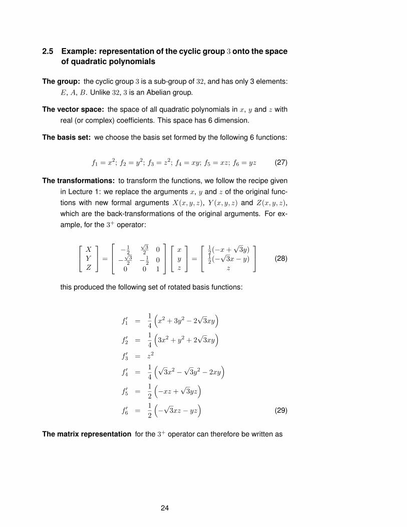
2.5 Example: representation of the cyclic group 3 onto the spaceof quadratic polynomials

The group: the cyclic group 3 is a sub-group of 32, and has only 3 elements:E, A, B. Unlike 32, 3 is an Abelian group.

The vector space: the space of all quadratic polynomials in x, y and z withreal (or complex) coefficients. This space has 6 dimension.

The basis set: we choose the basis set formed by the following 6 functions:

f1 = x2; f2 = y2; f3 = z2; f4 = xy; f5 = xz; f6 = yz (27)

The transformations: to transform the functions, we follow the recipe givenin Lecture 1: we replace the arguments x, y and z of the original func-tions with new formal arguments X(x, y, z), Y (x, y, z) and Z(x, y, z),which are the back-transformations of the original arguments. For ex-ample, for the 3+ operator:

XYZ

=

−12

√3

2 0

−√

32 −1

2 00 0 1

xyz

=

12(−x+

√3y)

12(−√

3x− y)z

(28)

this produced the following set of rotated basis functions:

f ′1 =1

4

(x2 + 3y2 − 2

√3xy

)f ′2 =

1

4

(3x2 + y2 + 2

√3xy

)f ′3 = z2

f ′4 =1

4

(√3x2 −

√3y2 − 2xy

)f ′5 =

1

2

(−xz +

√3yz)

f ′6 =1

2

(−√

3xz − yz)

(29)

The matrix representation for the 3+ operator can therefore be written as

24

14

34 0

√3

4 0 034

14 0 −

√3

4 0 00 0 1 0 0 0

−√

32 +

√3

2 0 −12 0 0

0 0 0 0 −12 −

√3

2

0 0 0 0√

32 −1

2

(30)

By exchanging columns 3 & 4 and rows 3 & 4 (which is equivalent toexchanging f3 with f4 and f ′3 with f ′4), the matrix can be rewritten as

14

34

√3

4 0 0 034

14 −

√3

4 0 0 0

−√

32

√3

2 −12 0 0 0

0 0 0 1 0 0

0 0 0 0 −12 −

√3

2

0 0 0 0√

32 −1

2

(31)

which is in block-diagonal form. Note that on this particular basis setthe matrix is not unitary, and [3−] = [3+]−1 6= [3+]T , although [3−] is inthe same block-diagonal form (for a basis set with unitary matrix repre-sentation, see Problem 4 of Problem Sheet 1, since C3 is a subgroupof D3). The latter demonstrates that the representation is reducible.One can prove that all representations of Abelian groups can be fullyreduced to diagonal form.

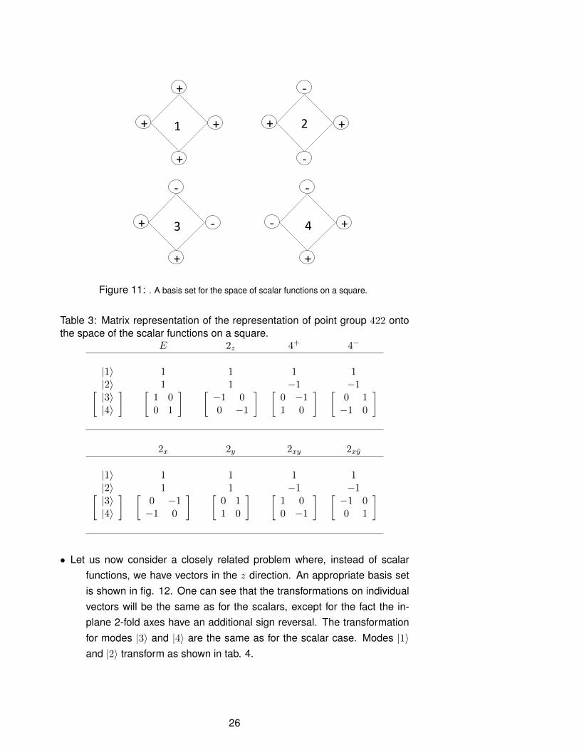
2.6 * Example: scalar functions on a square.

The group is 422 — the group of the square in 2D, which we have alreadyencountered. Note that this group is the same abstract group as thegroup of permutations of 4 objects (it has the same multiplication table).

The vector space: the space of all possible combinations of 4 numbers atthe corners of the square. It is a 4-dimensional space.

The basis set: we employ the basis set shown in fig. 11, where + and −indicates +1 and −1.

The matrix representation on this basis set is block-diagonal. Modes |1〉and |2〉 transform either into themselves or minus themselves by allsymmetry operators, and their matrix elements lie on the diagonal ofthe 4 × 4 matrix representation. Modes |3〉 and |4〉 are transformed ei-ther into themselves or into each other. This is illustrated in tab. 3.

25

+

++

+

-‐

++

-‐

-‐

-‐ +

+

-‐

+-‐

+

2 1

3 4

Figure 11: . A basis set for the space of scalar functions on a square.

Table 3: Matrix representation of the representation of point group 422 ontothe space of the scalar functions on a square.

E 2z 4+ 4−

|1〉 1 1 1 1|2〉 1 1 −1 −1[|3〉|4〉

] [1 00 1

] [−1 00 −1

] [0 −11 0

] [0 1−1 0

]

2x 2y 2xy 2xy

|1〉 1 1 1 1|2〉 1 1 −1 −1[|3〉|4〉

] [0 −1−1 0

] [0 11 0

] [1 00 −1

] [−1 00 1

]

• Let us now consider a closely related problem where, instead of scalarfunctions, we have vectors in the z direction. An appropriate basis setis shown in fig. 12. One can see that the transformations on individualvectors will be the same as for the scalars, except for the fact the in-plane 2-fold axes have an additional sign reversal. The transformationfor modes |3〉 and |4〉 are the same as for the scalar case. Modes |1〉and |2〉 transform as shown in tab. 4.

26

.

. .

.

.

xx

.

x

. x

.

x

x.

.

2 1

3 4

Figure 12: . A basis set for the space of z-vector functions on a square.

Table 4: Matrix representation of the representation of point group 422 ontothe space of the z-vector functions on a square.

E 2z 4+ 4−

|1〉 1 1 1 1|2〉 1 1 −1 −1

2x 2y 2xy 2xy

|1〉 −1 −1 −1 −1|2〉 −1 −1 1 1

3 Lecture 3: Key theorems about irreducible repre-sentations

• In the previous section, we have introduced the concepts of reducible andirreducible representations and seen some example of both. Abstractirreducible representations, or irreps for short, are extremely importantin both group theory and its applications in physics, and are governed bya series of powerful, one would be tempted to say “magical” theorems.Before we introduce them, we will start by asking ourselves a series ofquestions about irreps:

1. Are irreps a property of the group?

2. How many are they for a given group?

3. How can we characterise them, since for each there is clearly an

27

infinite number of matrix representations, all related by similaritytransformations?

4. How can we construct all of them?

5. How can we decompose a reducible representation in its irreducible(block-diagonal) “components”?

6. Once we have an irrep and one of its matrix representations, howcan we construct the corresponding basis vectors in a given space?

E A B K L M

Γ1 1 1 1 1 1 1

Γ2

1 1 1 -‐1 -‐1 -‐1

Γ3

312 2

3 12 2

⎛ ⎞− −⎜ ⎟⎜ ⎟+ −⎝ ⎠

1 00 1⎛ ⎞⎜ ⎟⎝ ⎠

1 00 1−⎛ ⎞⎜ ⎟⎝ ⎠

312 2

3 12 2

⎛ ⎞− +⎜ ⎟⎜ ⎟− −⎝ ⎠

312 2

3 12 2

⎛ ⎞+ −⎜ ⎟⎜ ⎟− −⎝ ⎠

312 2

3 12 2

⎛ ⎞+ +⎜ ⎟⎜ ⎟+ −⎝ ⎠

Point group 32 – variant 1

1

2

Figure 13: . A matrix representation for 3 irreps of for the point group 32 . The modes infig. 10 are basis vectors for Γ1 and Γ2. The appropriate basis vectors for Γ3 in the space ofordinary 2D vectors are indicated.

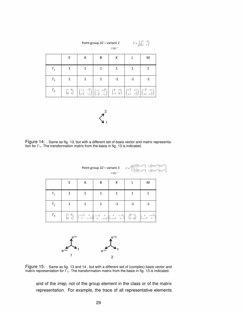
• To start answering these questions, let us look at 3 irreps of the point group32 we have already encountered (see figs 13, 14 and 15). The modes infig. 10 are basis vectors for Γ1 and Γ2, which are obviously irreduciblesince they are 1-dimensional. Γ3 is the “trivial” mapping onto the spaceof ordinary vector. We have not proven that this is an irrep, but let usassume it for the moment. Figs 13, 14 and 15 show 3 different matrixrepresentations (and basis vectors) for Γ3.

• We shall remember that 32 has 3 classes: {E}, {A,B} and {K,L,M}.

• We can verify explicitly the properties of the trace of the representativematrices, as explained above: the trace is a characteristic of the class

28

E A B K L M

Γ1 1 1 1 1 1 1

Γ2

1 1 1 -‐1 -‐1 -‐1

Γ3

312 2

3 12 2

⎛ ⎞− −⎜ ⎟⎜ ⎟+ −⎝ ⎠

1 00 1⎛ ⎞⎜ ⎟⎝ ⎠

0 11 0

−⎛ ⎞⎜ ⎟−⎝ ⎠

312 2

3 12 2

⎛ ⎞− +⎜ ⎟⎜ ⎟− −⎝ ⎠

3 12 2

312 2

⎛ ⎞+ +⎜ ⎟⎜ ⎟+ −⎝ ⎠

Point group 32 – variant 2

3 12 2

312 2

⎛ ⎞− +⎜ ⎟⎜ ⎟+ +⎝ ⎠

1 111 12

U−⎛ ⎞

= ⎜ ⎟⎝ ⎠

1UMU −

1

2

Figure 14: . Same as fig. 13, but with a different set of basis vector and matrix representa-tion for Γ3. The transformation matrix from the basis in fig. 13 is indicated.

E A B K L M

Γ1 1 1 1 1 1 1

Γ2

1 1 1 -‐1 -‐1 -‐1

Γ3

312 2

312 2

0

0

i

i

⎛ ⎞− +⎜ ⎟⎜ ⎟− −⎝ ⎠

1 00 1⎛ ⎞⎜ ⎟⎝ ⎠

0 11 0⎛ ⎞⎜ ⎟⎝ ⎠

Point group 32 – variant 3 ( ) ( )( ) ( )

3 12 2

3 12 2

1 123 1 1

i i i

i i i

e e eU

e e e

ω ω ω

ω ω ω

− − +

+ + −

⎛ ⎞− − + +⎜ ⎟=⎜ ⎟− − + +⎝ ⎠

312 2

312 2

0

0

i

i

⎛ ⎞− −⎜ ⎟⎜ ⎟− +⎝ ⎠

312 2

312 2

0

0

i

i

⎛ ⎞− −⎜ ⎟⎜ ⎟− +⎝ ⎠

312 2

312 2

0

0

i

i

⎛ ⎞− +⎜ ⎟⎜ ⎟− −⎝ ⎠

1UMU −

1

2

e-iω

e+iω 1

e+iω

e-iω 1

Figure 15: . Same as fig. 13 and 14 , but with a different set of (complex) basis vector andmatrix representation for Γ3. The transformation matrix from the basis in fig. 13 is indicated.

and of the irrep, not of the group element in the class or of the matrixrepresentation. For example, the trace of all representative elements

29

for {K,L,M} is 1 for Γ1, −1 for Γ2 and 0 for Γ3. As already mentioned,we call this trace the character of the irrep for a given class3. The setof characters will be used to characterise the irreps — see below fortheorems that put this on solid foundation.

• By examining each of the tables separately, we can determine the following:

� Let us construct 6 arrays, of 6 elements by taking the representativenumber of each operator for the 1D irreps Γ1 and Γ2 and one ofthe 4 elements of the representative matrices for the 2D irrep Γ3.For example, for the table in fig. 13 we get the following 6 arrays:

1 1 1 1 1 11 1 1 −1 −1 −11 −1

2 −12 −1 +1

2 +12

0 −√

32 +

√3

2 0 −√

32 +

√3

2

0 +√

32 −

√3

2 0 −√

32 +

√3

21 −1

2 −12 1 −1

2 −12

(32)

� The 6 arrays are orthogonal with each other (in the ordinary senseof orthogonality of arrays).

� The norm of each array is√

6 for Γ1 and Γ2 and√

3 for Γ3, which canall be written as

√h/lj , where h is the number of elements in the

group and lj is the dimension of the irrep.

• We can verify that the same properties apply to the table in figs 14, althoughthe arrays for Γ3 are clearly different.

• We can also verify that the same properties apply to the table in fig 16,which contains 5 irreps of the point group 422.

• The table in figs 15, is slightly different, because the matrix elements arecomplex4. The 6 arrays are:

3Note that all the characters for all the irreps of this group and group 422 below are real.We can prove that if g ∼ g−1, then the character of any unitary representation of g is real.In fact, g ∼ g−1 → U(g) = MU−1(g)M−1 = MU†(g)M−1. Taking the trace, tr(U(g)) =tr(U∗(g)) = tr∗(U(g)), so the character is real. g ∼ g−1 for all operators in 32 and 422.

4Somewhat surprisingly, this is the standard setting for these matrices, as shown, forexample, in http://www.cryst.ehu.es/rep/point.html. The reason is that the cyclic subgroup ofD3, C3, is Abelian, and all the representations of an Abelian group can be fully reduced into1D irreps, which usually have complex characters. The one shown here is the basis that fullyreduces C3. For Abelian groups, each element is in a class of its own, so it obviously cannotbe g ∼ g−1 unless g = g−1.

30

1 1 1 1 1 11 1 1 −1 −1 −1

1 −12 + i

√3

2 −12 − i

√3

2 0 0 0

0 0 0 −12 − i

√3

2 1 −12 + i

√3

2

0 0 0 −12 + i

√3

2 1 −12 − i

√3

2

1 −12 − i

√3

2 −12 + i

√3

2 0 0 0

(33)

• One can verify that line 3 is actually orthogonal to the complex conjugateof line 6 etc.

• Remembering that each array element is actually an element of the repre-sentative matrix of an irrep, we can summarise all these results as anorthogonality relation:

∑g

D(g)ΓiµνD

∗(g)Γj

µ′ν′ =h

liδijδµµ′δνν′ (34)

E 2z 4+ 4-‐ 2x 2y 2xy 2xy

Γ1 1 1 1 1 1 1 1 1

Γ2

1 1 1 1 -‐1 -‐1 -‐1 -‐1

Γ3

1 1 -‐1 -‐1 1 1 -‐1 -‐1

Γ4

1 1 -‐1 -‐1 -‐1 -‐1 1 1

Γ5

Point group 422 (one of the variants)

1 00 1⎛ ⎞⎜ ⎟⎝ ⎠

1 00 1−⎛ ⎞⎜ ⎟−⎝ ⎠

0 11 0

−⎛ ⎞⎜ ⎟⎝ ⎠

0 11 0

⎛ ⎞⎜ ⎟−⎝ ⎠

1 00 1⎛ ⎞⎜ ⎟−⎝ ⎠

1 00 1−⎛ ⎞⎜ ⎟⎝ ⎠

0 11 0⎛ ⎞⎜ ⎟⎝ ⎠

0 11 0

−⎛ ⎞⎜ ⎟−⎝ ⎠

Figure 16: . A matrix representation for 5 irreps of for the point group 422 .

• The orthogonality relation in eq. 34 can be easily converted into an or-thonormality relation by normalising all the arrays with the coefficient√lj/h.

31

3.1 The Wonderful Orthogonality Theorem and its implications

• Amazingly, eq. 34 represents a general theorem applicable to all uni-tary matrix representations of all irreps of all finite groups. This isthe so-called Wonderful Orthogonality Theorem (WOT), due to physi-cist and Nobel prize winner John Van Vleck (this tells a story of its ownabout the importance of group theory in the early days of quantum the-ory). The theorem can be easily extended to non-unitary matrix rep-resentations (see Dresselhaus, p 25, eq. 2.52), but we will be contenthere with its version for unitary representations. The proof of the WOTis not conceptually difficult, but it is rather convoluted. One proves theso-called Schur’s Lemma (in 2 parts) to begin with, then moves to theactual proof. This is done in detail in Dresselhaus, pp 21-27.

• It is important to stress that the WOT is only valid for irreducible represen-tations. Indeed, if a representation is reducible, the matrix elements ofany of its matrix representations will not be orthogonal to those of theirreps it can be decomposed into.

• The importance of the WOT cannot be overestimated, since it goes a longway to answer the questions stated at the beginning of this section.

• One can immediately see that the number of irreps of a given group andtheir dimensionality is limited by the fact that only h mutually orthogonalvectors can be constructed in the space of arrays of dimensionality h.Since the number of such arrays arising from a given irrep of dimensionlj is l2j , it must be:

∑j

l2j ≤ h (35)

As we will see later it is the strict = sign that holds in eq. 35.

3.2 The Wonderful Orthogonality Theorems for Characters

• We can go even further by constructing the so-called character tables,which can be done for the full group or for the classes (remember thatgroup elements in the same conjugation class have the same char-acters, since their representative matrices are similar). For example,group 32 has the character tables shown in fig. 17.

• Turning our attention first to the full-group table, we can see that each ele-ment is simply:

32

E A B K L M

Γ1 1 1 1 1 1 1

Γ2

1 1 1 -‐1 -‐1 -‐1

Γ3

2 -‐1 -‐1 0 0 0

Point group 32 – Character Table (full group)

E 2A 3K

Γ1 1 1 1

Γ2

1 1 -‐1

Γ3

2 -‐1 0

Point group 32 – Character Table(classes)

Figure 17: Character tables for the point group 32 . In the class table, the number precedingthe representative element (e.g., 2A, 3K), indicates the number of elements in the class.

tr(D(g)Γi) =∑µ

D(g)Γiµµ (36)

• The three arrays in the table must remain orthogonal to each other becauseof the way they are constructed. For example, the array correspondingto Γ3 is:

[2 −1 −1 0 0 0

]=

[1 −1

2 −12 −1 +1

2 +12

]+

[1 −1

2 −12 +1 −1

2 −12

](37)

the arrays to the right of the = sign being arrays 3 and 6 in eq. 32.Since these are orthogonal to all the other arrays in eq. 32, their summust also be orthogonal. However, the normalisation has now changed,since the squared norm of these arrays will be multiplied by lj . If weindicate with χ(g)Γi the character of group element g in irrep Γi, weobtain the following WOT for characters - full group version.

33

∑g

χ(g)Γiχ∗(g)Γj = hδij (38)

• This can be easily modified for application to the class version of the char-acter table, e.g., fig. 17 (bottom panel). All the element in each classhave the same character, so if we call Nk the number of group ele-ments in class Ck (for clarity, this is usually indicated in class charactertables such as fig. 17 — bottom panel), eq. 38 becomes the WOT forcharacters - classes version:

∑k

Nkχ(Ck)Γiχ∗(Ck)

Γj = hδij (39)

• Once again, one can easily construct orthonormal arrays of dimensionalityequal to the number of classes by normalising each array. The arrays

[√N1

hχ(C1)Γi ,

√N2

hχ(C2)Γi , · · ·

√Nn

hχ(Cn)Γi

](40)

are orthonormal for different i’s.

• Eq. 39 further restricts the number of irreps for a group. If the number ofclasses is n, the number of independent mutually orthogonal vectors ofdimension n is at most n, so it must be

Nirreps ≤ Nclasses (41)

where, once again, the strictly = sign holds (see below).

3.3 Reducible representations and their decomposition

• The trace of a block-diagonal matrix is the sum of the traces of itsdiagonal blocks. This is quite obvious from the definition of the trace.If a representation is reducible, the representative matrices of all thegroup elements can be written in the same identical diagonal form. Itfollows that the array of characters of a reducible representation isa linear combination of the character arrays of the irreps of thegroup. Calling the reducible representation Γred:

[χ(g1)Γred , χ(g2)Γred , · · ·χ(gh)Γred

]=∑i

ai[χ(g1)Γi , χ(g2)Γi , · · ·χ(gh)Γi

](42)

34

or

[χ(C1)Γred , χ(C2)Γred , · · ·χ(Cn)Γred

]=∑i

ai[χ(C1)Γi , χ(C2)Γi , · · ·χ(Cn)Γi

](43)

• The coefficients ai are integers indicating the number of times irrep Γi

appears in the decomposition of reducible representation Γ — inother words, the number of identical (or better similar) diagonal blockscorresponding to irrep Γi along the diagonal, once Γ is fully decom-posed.

• Eq. 42 can be inverted exploiting the orthonormality relation, to find thecoefficients:

aj =1

h

∑g

[χ(g)Γj

]∗χ(g)Γred (44)

or, for classes

aj =∑k

Nk

h

[χ(Ck)

Γj]∗χ(Ck)

Γred (45)

Example: let us look again at the example given on page 21 — the rep-resentation of 32 on the space of triangular distortions. This is a 6-dimensional reducible representation of 32. We have already found 3irreps for 32 (see fig. 17), and we know that we cannot have more than3, since 32 has 3 classes (eq. 41), so we can be confident we havefound all the 32 irreps. We can also see that

∑j

l2j = 12 + 12 + 22 = 6 = h (46)

The character array for Γred is (just take the trace of all matrices):

E A B K L M6 0 0 0 0 0

by applying eq. 44 we obtain

a1 = 1; a2 = 1; a3 = 2 (47)

35

We write:Γred = Γ1 + Γ2 + 2Γ3 (48)

which means that Γ1 and Γ2 appear once in the decomposition of Γred, whileΓ3 appears twice.

3.4 Second WOT for characters and number of irreps

• We have seen that rows of the matrix:

[√N1h χ(C1)Γ1 ,

√N2h χ(C2)Γ1 , · · ·

√Nnh χ(Cn)Γ1

][√

N1h χ(C1)Γ2 ,

√N2h χ(C2)Γ2 , · · ·

√Nnh χ(Cn)Γ2

]· · ·[√

N1h χ(C1)Γn ,

√N2h χ(C2)Γn , · · ·

√Nnh χ(Cn)Γn

](49)

are orthonormal arrays.

• It can also be easily proven (Dresselhaus, pp 36–37) that the colums ofthis matrix are orthonormal. This is the second WOT for characters,which can also be written as

∑i

χ(Ck)Γi[χ(Ck′)

Γi]∗

=h

Nkδkk′ (50)

This time, the summation is over irreps, not over group elements asbefore.

• By using the second WOT for characters, we can prove that Nirreps =

Nclasses. In fact, we have constructed Nclasses independent and or-thonormal arrays of dimension Nirreps, and in order to do this it mustbe Nirreps ≥ Nclasses. However, we have already seen that Nirreps ≤Nclasses, which implies Nirreps = Nclasses.

3.5 * Construction of all the irreps for a finite group

• We illustrate one method to construct all irreps of a given group. Thismethod is not the one employed in actual fact, but it is useful becauseis simple and enables us to prove that

∑j l

2j = h.

36

• Let’s consider the multiplication table of the group, as exemplified by fig.5 for our usual group 32, and let’s rearrange the order or rows andcolumns so that all the identity elements E fall on the diagonal, as infig. 18. It is easy to see that this is always possible for any finite group.

D3 (32)

E B A K L M

E E B A K L M

A A E B L M K

B B A E M K L

K K L M E B A

L L M K A E B

M M K L B A E

Applied first

App

lied

seco

nd

Figure 18: Multiplication table for the point group 32 (D3), rearranged to contract the regularrepresentation.

• We then construct the so-called regular representation, as follows: thematrix representative of group element g is obtained by replacing the gentries of the multiplications table with 1’s and all the other entries with0’s. For example, in fig. 18, the representative matrix of element K isobtained by replacing all K’s in the table with 1’s and all the other letterswith 0’s.

• One can verify that the regular representation is in fact a representation —in particular it respects the composition – matrix multiplication relation.

• The regular representation has dimension h and is reducible. Its charactersare h for the identity and 0 for all the other elements.

• By applying the decomposition formula we obtain:

aj =1

h

∑g

[χ(g)Γj

]∗χ(g)Γreg = lj (51)

since the character of the identity for a reducible or irreducible repre-sentation is equal to its dimension. In other words each irrep is rep-resented a number of times equal to its dimension in the regularrepresentation.

37

• It is therefore possible in principle to obtain all the irreps of a given group byblock-diagonalising all the matrices of the regular representation (this isnot what is done in practice).

• More usefully, since the dimension of Γreg is h, and the dimension of areducible representation is the sum of the dimension of its irreps timesthe number of times they appear, it must be:

∑j

l2j = h (52)

as we set out to prove.

• All the irreps of the 32 crystallographic point groups have been determinedmany years ago, and can be found (including one standard setting forthe matrices) at the following address: http://www.cryst.ehu.es/rep/point.html.

4 Lecture 4: Applications of representations to physicsproblems

4.1 Quantum mechanical problems: the symmetry of the Hamil-tonian

• Let us first recall our definition of symmetry transformations for functionsand their gradients from Section 1.2.1:

g[f(x)] = f(R−1(g)x)

g[∇f(x)] = (R(g)∇) f(R−1(g)x) (53)

we have not proven explicitly the second line of eq. 53 , but its derivationis simple and completely general for vector functions.

• Since all transformations we are interested in here are isometric (i.e., pre-serve the norm) it also follows that

g[∇2f(x)] = ∇2f(R−1(g)x) (54)

• As introduced in eq. 14, the mapping g → O(g) ∀g ∈ G defines a repre-sentation of the group G onto the Hilbert space. The operators O(g) areunitary : therefore, they possess orthonormal eigenvectors with eigen-values on the unit circle in complex space.

38

• Now we want to show explicitly that if the Hamiltonian is invariant by atransformation g as defined in eq. 53, then the operator O(g) commuteswith the Hamiltonian:

O(g)Hψ(x) =

(−∇

2

2m+ U(R−1(g)x)

)ψ(R−1(g)x)

HO(g)ψ(x) =

(−∇

2

2m+ U(x)

)ψ(R−1(g)x) (55)

so it is in fact necessary and sufficient for the potential to be invariantby the symmetry g to ensure that the Hamiltonian commutes with O(g).This relation between symmetry invariance and commutation is in gen-eral true for any quantum-mechanical Hermitian operator, not only forthe Hamiltonian.

• Let us now assume that the Hamiltonian is invariant for all elements of thegroup G, i.e., that it commutes with all the operators O(g)∀g ∈ G. Thefollowing statements can be readily proven (they can in fact be extendedto any Hermitian operator that has the symmetry of the group G):

1. If φ(x) is an eigenstate of H with eigenvalue λ, then all O(g)φ(x)

are also eigenstates of H with the same eigenvalue λ, and this∀g ∈ G. In fact,

HO(g)φ(x) = O(g)Hφ(x) = λO(g)φ(x) (56)

2. If φ(x) is a non-degenerate eigenstate of H, then the map g →O(g) onto the one-dimensional subspace defined by φ(x) is a one-dimensional irreducible representation ofG. In fact, since the eigen-vector is non-degenerate, it must necessarily be O(g)φ(x) = cφ(x) ∀g,c being a unitary constant, and this is precisely the definition of aone-dimensional irreducible representation.

3. If φ1(x) . . . φn(x) are degenerate eigenstates of H defining a sub-space of the Hilbert space of dimension n, then the map g → O(g)

onto that subspace defines an n-dimensional representation of {g}If the degeneracy is not accidental and there is no additional sym-metry, then the representation is irreducible. In fact, since for everyφi(x) of the degenerate subspace and for every g, O(g)φi(x) is aneigenstate with the same eigenvalue, so

O(g)φi(x) =∑j

cjφj(x) (57)

39

Therefore the application of O(g) is closed within the φi(x) sub-space, and is therefore a representation of the group G.

4. With regards to the question of whether this representation is re-ducible or irreducible, we will just give here some qualitative ar-guments. If the representation was reducible, then we could splitthe subspace defined by the φi(x) into two or more subspaces,each closed upon application of the operators O(g), but both withthe same eigenvalues. If there is no additional symmetry, one canimagine changing the Hamiltonian adiabatically (and without alter-ing its symmetry) in such a way that the eigenvalues of the twoor more subspace become different — in other words, the degen-eracy of the two subspaces would be accidental. On the otherhand, if the Hamiltonian has additional symmetries, the reduciblesubspace by the first symmetry group may be irreducible by thesecond symmetry group, so that two or more irreducible represen-tations of the first group may be “joined” together into multiplets (aclassic case is that of the exchange multiplets in magnetism).

• We conclude that, in general, the complete orthogonal basis set ofeigenstates of the Hamiltonian fully reduces the representationg → O(g) of the symmetry group of the Hamiltonian.

• It is important to note that the reverse is not true — in other words, a ba-sis set that fully reduces the representation g → O(g) is not necessarilya set of eigenstates for the Hamiltonian. The problem arises when aparticular irreducible representation Γ of the group {g} appears morethan once in the decomposition of the representation g → O(g).

Example; let’s consider two sets of eigenstates, φ1(x) . . . φn(x) with eigen-value λ1 and ψ1(x) . . . ψn(x), with eigenvalue λ2. Let us also assumethat both sets transform with the same irreducible matrix representationΓi, which would therefore appear more than once in the decompositionof g → O(g). It is easy to see that the set aφ1(x) + bψ1(x) . . . aφn(x) +

bψn(x) (a and b being complex constants) also transforms with the sameirreducible representation — in fact with the same matrices as the origi-nal two sets. However, it is also clear that the new basis set is not a setof eigenstates of H.

• Therefore, in the presence of irreducible representations that appear morethan once, more work is required to extract eigenstates from basis func-tions of irreducible representations (which can be obtained by the appli-cation of the projection operator — see below).

40

• Nevertheless, structuring the Hilbert space in terms of invariant subspacesby the irreps of the symmetry group of the Hamiltonian provides anenormous simplification to the solution of the Schroedinger equation,and defined a natural connection between problems having differentpotentials but the same symmetry group.

4.2 * Classical eigenvalue problems: coupled harmonic oscilla-tors

• The same techniques can be applied with hardly any modifications to clas-sical eigenvalue problems, since the mathematical formalism is identi-cal to that of the quantum case. Classical eigenvalue problems are rele-vant to many CMP systems, for example, molecular vibrations, phononsin crystals, but also classical spin waves.

• As an example, we present the case of molecular vibrations. We start withthe expression for the kinetic and potential energies in the limit of “small”displacements from the equilibrium position.

EK =1

2

∑i

mix2

EP =1

2

∑i,j

∂2U

∂xi∂xjxixj (58)

Here, the xi’s are the displacement coordinates of ion i and mi are theirmass. The sum runs over both ions and components. The analysisproceeds in the following steps:

1. We perform a transformation to the reduced coordinates:

ξi = xi√mi (59)

This has the effect of eliminating the masses from the kinetic en-ergy expression:

EK =1

2

∑i

ξ2

EP =1

2

∑i,j

(1

√mimj

∂2U

∂xi∂xj

)ξiξj (60)

41

2. We write the equation of motion as:

ξi +∑j

(1

√mimj

∂2U

∂xi∂xj

)ξj = 0 (61)

3. We seek solution of the form

ξi = qi eiωt (62)

from which we derive the secular equation

ω2qi =∑j

(1

√mimj

∂2U

∂xi∂xj

)qj =

∑j

Vijqj (63)

Eq. 63 is usually solved by diagonalising the matrix Vij on theright-hand side.

• We want to show that symmetry analysis simplifies the solution of this prob-lem very significantly.

• First of all, we define our vector space as the space of all modes, definedas [q1x, q1y, q1z, q2x · · · ]. The dimension of the space is mD, where m

is the number of atoms in the molecule and D is the dimension of the(ordinary) space.

• We can define a (reducible) representation Γ of the symmetry group of thepotential energy U onto this vector space as the symmetry transforma-tion of the modes, involving both a change of the atom labelling and ofthe components. This is completely analogous to the example in sec-tion 2.4 (representation of the group 32 onto the space of distortions ofa triangle).

• One can show explicitly that the invariance of U by the symmetry group Gimplies that Vij commutes with all the representative matrices.

• From here onward, we can follow the quantum derivation step by step. Inparticular, we conclude that the eigenvectors of Vij provide an irre-ducible decomposition of Γ in terms of the irreps of G. In particular, themultiplet structure of the solution is deduced entirely by symme-try. If an irrep Γi appears more than once in the decomposition of Γ,the eigenvectors of Vij will not be determined entirely by symmetry, butone will have to diagonalise a much smaller matrix to find them.

42

4.3 Extended example: normal modes of the square molecule

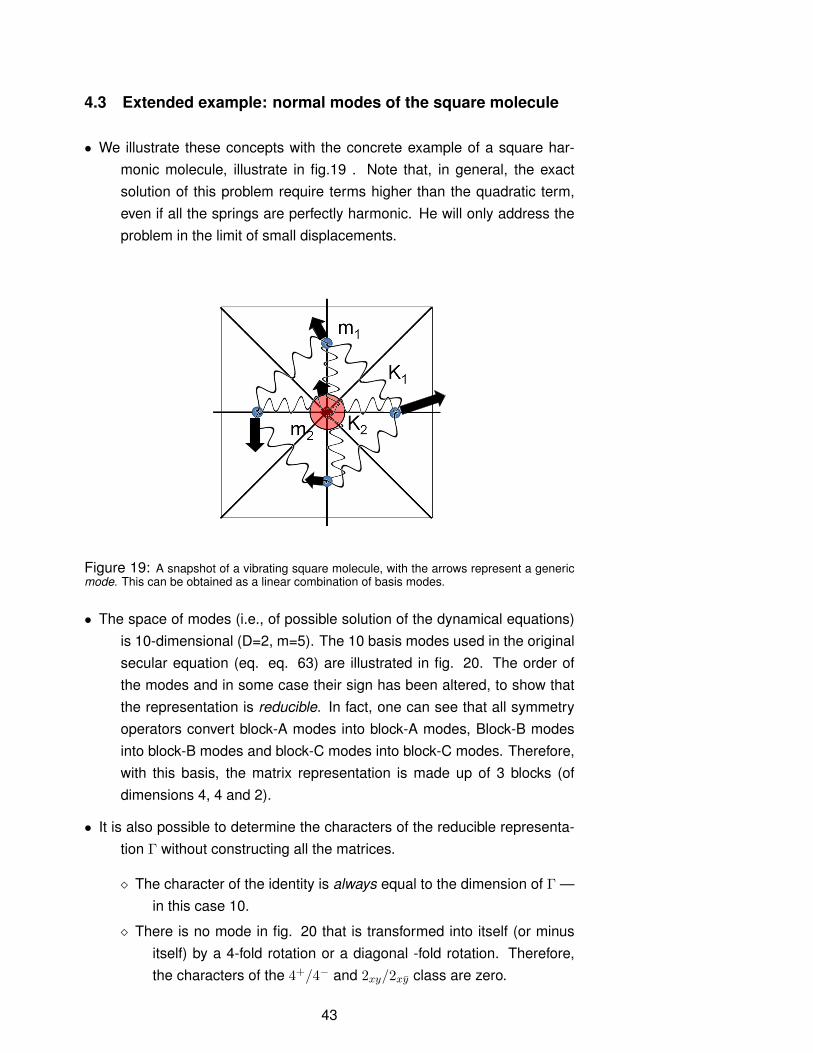
• We illustrate these concepts with the concrete example of a square har-monic molecule, illustrate in fig.19 . Note that, in general, the exactsolution of this problem require terms higher than the quadratic term,even if all the springs are perfectly harmonic. He will only address theproblem in the limit of small displacements.

Figure 19: A snapshot of a vibrating square molecule, with the arrows represent a genericmode. This can be obtained as a linear combination of basis modes.

• The space of modes (i.e., of possible solution of the dynamical equations)is 10-dimensional (D=2, m=5). The 10 basis modes used in the originalsecular equation (eq. eq. 63) are illustrated in fig. 20. The order ofthe modes and in some case their sign has been altered, to show thatthe representation is reducible. In fact, one can see that all symmetryoperators convert block-A modes into block-A modes, Block-B modesinto block-B modes and block-C modes into block-C modes. Therefore,with this basis, the matrix representation is made up of 3 blocks (ofdimensions 4, 4 and 2).

• It is also possible to determine the characters of the reducible representa-tion Γ without constructing all the matrices.

� The character of the identity is always equal to the dimension of Γ —in this case 10.

� There is no mode in fig. 20 that is transformed into itself (or minusitself) by a 4-fold rotation or a diagonal -fold rotation. Therefore,the characters of the 4+/4− and 2xy/2xy class are zero.

43

1

2

4

3

[1x] 1

2

4

3

[2y]

1

2

4

3

[-3x]

1

2

4

3

[-4y]

1

2

4

3

[1y] 1

2

4

3

[-2x]

1

2

4

3

[-3y] 1

2

4

3

[4x]

A

B

C

Figure 20: The 10 modes in the square molecule dynamical matrix, slightly rearranged toshow that the representation can be reduced.

� Some modes are transformed into themselves or minus themselvesby the in-plane 2-fold axes. For example the two right-hands modesin block A are invariant by 2y, while those on the left side are invari-ant by 2x. Likewise, modes in block B are multiplied by −1 by thesame transformation. However, since +1 and −1 always appear inpairs along the diagonal of the representative matrices, their traceis zero.

� Modes in blocks A and B are never transformed into themselves (orminus themselves) by 2z. However, modes in block C are alwaystransformed into minus themselves. Therefore the trace of the ma-trix representation of 2z is −2.

� The character table of Γ is therefore:

E 2z 2(4+) 2(2x) 2(2xy)

10 -2 0 0 0

• Point group 422 has 5 classes and 5 irreps. Their dimensions are 1, 1, 1, 1

and 2, since12 + 12 + 12 + 12 + 12 + 22 = 8 = h.

• The character table can be constructed, for example, from fig. 16:

44

E 2z 2(4+) 2(2x) 2(2xy)

Γ1 1 1 1 1 1Γ2 1 1 1 -1 -1Γ3 1 1 -1 1 -1Γ4 1 1 -1 -1 1Γ5 2 -2 0 0 0

• By applying eq. 45 or simply by inspection, one can decompose Γ into itsirreducible components:

Γ = Γ1 + Γ2 + Γ3 + Γ4 + 3Γ5 (64)

• As one can see, 1-dimensional irreps Γ1, Γ2, Γ3 and Γ4 only appear once inthe decomposition. Modes that transform according to these irrepswill therefore be automatically normal modes, regardless to theexact form of the potential matrix.

• These modes are easy to construct by hand, without using the projectors.They are shown in fig. 21 .

• Mode Γ4 has clear zero frequency (is a pure rotation in the limit of smalldisplacements). The frequency of the other modes can be obtained byequating the potential energy at maximum stretch with the kineticenergy at zero stretch, both proportional to the square of the amplitudeof the mode in the small-displacement limit.

• The remaining 6 normal modes all transform in pairs according to Γ5. Oneof the pairs is made up of pure translation of the molecule, and has zerofrequency. The other two modes have non-zero frequencies, and havethe form shown in fig. 24.

• One can see that these are generic linear combinations of the modesshown in fig. 22 and 23, with the further constraint that the centre-of-mass motion can be set to zero. The problem has been thereforereduced to 2 coupled equations, as opposed to the original 10.

5 Lecture 5: Projectors, subduction and group prod-uct

In this section, we will finally answer question 6 on page 28, by constructingthe projection operators (projectors), which will enable us to generate the

45

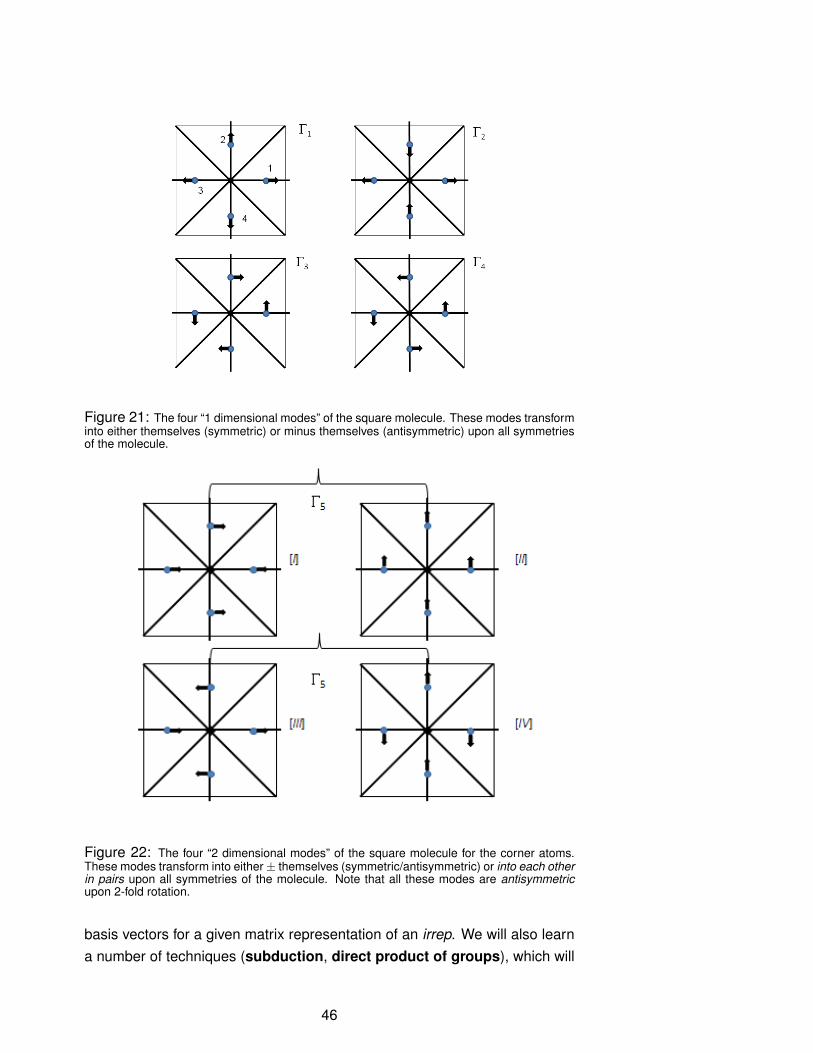
Figure 21: The four “1 dimensional modes” of the square molecule. These modes transforminto either themselves (symmetric) or minus themselves (antisymmetric) upon all symmetriesof the molecule.

Figure 22: The four “2 dimensional modes” of the square molecule for the corner atoms.These modes transform into either± themselves (symmetric/antisymmetric) or into each otherin pairs upon all symmetries of the molecule. Note that all these modes are antisymmetricupon 2-fold rotation.

basis vectors for a given matrix representation of an irrep. We will also learna number of techniques (subduction, direct product of groups), which will

46

Figure 23: The two central-atom modes of the square molecule. One can verify that theytransform as the ”2-D” corner modes, i.e., with the representation Γ5

Figure 24: Examples of non-zero-frequency normal modes of Γ5 symmetry involving two-atom displacements. The exact mixing coefficient depend on the mass and spring constantparameters.

47

help to construct representations and decompose them into irreps for severalphysically relevant problems.

5.1 Projectors

• As the name suggests, projectors project an arbitrary element of the vectorspace onto the basis vectors of a given matrix representation of an irrep.

• Because of this, projectors depend on the particular choice of matrix rep-resentation, and one therefore needs the full matrix (not just the char-acters) to construct them.

• Projectors are operators (not matrices). In fact they are linear combinationsof the operators O(g) for all the elements of the group.

• The coefficient of the linear combination are related to the matrix elementsDΓiµν(g), in other words, the matrix elements of a specific matrix repre-

sentation of the irrep Γi. More precisely:

PΓiµν =

lih

∑g

[DΓiµν(g)

]∗O(g) (65)

• Note that there will be l2j projectors for an irrep of dimension lj , so there isa lot of redundancy in the way projectors can be constructed.

• By employing the WOT, one can find out how projectors work. Let

v =∑

i = 1, · · ·nκ = 1, · · · li

aiκviκ (66)

be a generic vector in the vector space. The sum over j runs over theirreps, while the sum over κ runs over the different basis vector of agiven irrep and matrix representation. If each irrep is represented nomore than once in the decomposition, one can show that

PΓiµνv = aiνviµ (67)

In the case of multiple instances of the same irrep, the formula is

PΓiµνv =

∑p

apiνvpiµ (68)

where the sum over p is over the multiple instances of Γi.

48

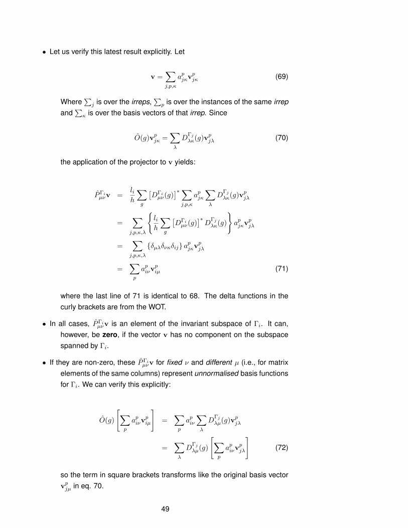
• Let us verify this latest result explicitly. Let

v =∑j,p,κ

apjκvpjκ (69)

Where∑

j is over the irreps,∑

p is over the instances of the same irrepand

∑κ is over the basis vectors of that irrep. Since

O(g)vpjκ =∑λ

DΓj

λκ(g)vpjλ (70)

the application of the projector to v yields:

PΓiµνv =

lih

∑g

[DΓiµν(g)

]∗∑j,p,κ

apjκ∑λ

DΓj

λκ(g)vpjλ

=∑j,p,κ,λ

{lih

∑g

[DΓiµν(g)

]∗D

Γj

λκ(g)

}apjκv

pjλ

=∑j,p,κ,λ

{δµλδνκδij} apjκvpjλ

=∑p

apiνvpiµ (71)

where the last line of 71 is identical to 68. The delta functions in thecurly brackets are from the WOT.

• In all cases, PΓiµνv is an element of the invariant subspace of Γi. It can,

however, be zero, if the vector v has no component on the subspacespanned by Γi.

• If they are non-zero, these PΓiµνv for fixed ν and different µ (i.e., for matrix

elements of the same columns) represent unnormalised basis functionsfor Γi. We can verify this explicitly:

O(g)

[∑p

apiνvpiµ

]=

∑p

apiν∑λ

DΓj

λµ(g)vpjλ

=∑λ

DΓj

λµ(g)

[∑p

apiνvpjλ

](72)

so the term in square brackets transforms like the original basis vectorvpjµ in eq. 70.

49

5.2 Example of use of the projectors: distortions on a triangles(the “ozone” molecule)

• We can put these concepts into practice by examining a problem we havealready encountered multiple times — that of the distortions (vibrations)of a triangle. This is often dubbed the “ozone molecule” problem, al-though the actual ozone (O3) molecule is an isosceles triangle with theobtuse angle equal to 116.8◦. The formalism is, however, suitable tostudy actual molecules such as SO3 and BF3. We will only consider thedisplacements of the external atoms, which form a perfect equilateraltriangle in the ground state.

• We have essentially all the elements already in place to discuss this prob-lem. The basis vectors of the reducible representation, shown in fig. 9page 23, span a 6-dimensional space. Hereafter, we will indicate thesemodes with |1〉 · · · |6〉. The full matrices on these basis vectors are dis-played in eq. 26 page 22. We have already decomposed the reduciblerepresentation into irreps as Γred = Γ1 + Γ2 + 2Γ3 (eq. 48 page 36).The two basis vectors for the 1-dimensional irreps were found by trialand error, and are shown in fig. 10 page 23. We will indicate these twomodes as |Γ1〉 and |Γ2〉. Finally, we have several variants of the matrixrepresentations (figs 13, 14, 15 ) but we will only employ Variant 1 forthe projectors (fig. 13 page 28). The character table is on fig. 17 page33.

• We will start by applying PΓ1 to modes |1〉 · · · |6〉. There is only one projec-tor for Γ1, since the irrep is 1-dimensional, and all the coefficients in eq.65 are 1, since this is the totally symmetric representation. It is easy toshow that

PΓ1 |1〉 = PΓ1 |2〉 = PΓ1 |3〉 =1

3|Γ1〉

PΓ1 |4〉 = PΓ1 |5〉 = PΓ1 |6〉 = 0 (73)

Likewise

PΓ2 |1〉 = PΓ2 |2〉 = PΓ2 |3〉 = 0

PΓ2 |4〉 = PΓ2 |5〉 = PΓ2 |6〉 =1

3|Γ2〉 (74)

50

So we have easily obtained the basis vectors of the to 1-dimensionalirreps by projection. As in the previous cases, these are automaticallynormal modes. Γ2 represents a pure rotation and has zero frequency.

• The situation is somewhat more complicated for Γ3: this irrep is 2-dimensional(so we have 4 projectors), it appears twice in the decomposition and wedo not know the answers in advance. To simplify the problem slightly,we can look the full matrix irrep in fig. 13 and note that the matrix foroperator K is diagonal, with the first mode being antisymmetric andthe second symmetric. Since mode |2〉 and |5〉 are also symmetric andantisymmetric by K , respectively, projecting these two modes will re-sult in a simpler combination of modes. In fact, PΓ3

µν v projects ontomode µ with the coefficient of mode ν in the decomposition of v.Since |2〉 is symmetric, there will be no antisymmetric component in itsdecomposition, so

PΓ311 |2〉 = PΓ3

21 |2〉 = 0

PΓ312 |5〉 = PΓ3

22 |5〉 = 0 (75)

• The modes generated by application of the projectors to modes |2〉 and |5〉are shown in fig. 25. In particular, one can verify directly the relationsin eq. 75 and

PΓ311 |5〉 =

1

3|m1〉

PΓ312 |2〉 =

1

3|m′1〉

PΓ321 |5〉 =

1

3|m2〉

PΓ322 |5〉 =

1

3|m′2〉 (76)

• Modes |m1〉 and |m2〉 form a basis set for the chosen matrix representationof Γ3, and so do modes |m′1〉 and |m′2〉. This is consistent with the gen-eral rule that PΓi

µνv for fixed ν and different µ represent unnormalisedbasis functions for Γi.

• This is as much as one can say by employing symmetry considerations. Itis not possible to make more progress towards determining the normalmodes without employing some physical considerations. Since modes

51

m1 m2

m'1 m’2

2

1

1

1 1

2

√3 √3

√3 √3

Γ3

Γ3

Figure 25: Modes generated by |2〉 and |5〉 through the application of the projectors. Thelength of the arrows is indicated.

|m1〉, |m2〉, |m′1〉 and |m′2〉, intended as vibration modes, do not con-serve the centre of mass, one can try the following linear combinations:

|n1〉 =|m1〉 − |m′1〉

2

|n2〉 =|m2〉 − |m′2〉

2

|n′1〉 =|m1〉+ |m′1〉

2

|n′2〉 =|m2〉+ |m′2〉

2(77)

These modes are shown in fig. 26, and are in fact the remaining normalmodes of the triangular molecule. Modes |n1〉 and |n2〉 the are puretranslations, and have zero frequency.

5.3 Subduction

• One of the most useful application of the theory of representations is in thestudy of spectroscopic splittings. Let ’s imagine a Hamiltonian of theform:

52

n1 n2

n'1 n’2

1

Γ3

Γ3

Figure 26: The Γ3 normal modes of the triangulate molecule. The relation between thesemodes and those in fig. 25 is shown in eq. 77.

H = H0 + λH1 (78)

where λ is a small parameter, H0 has symmetry group G0, while H1

(and therefore H) have symmetry group G1 ⊂ G0, i.e., G1 is a propersubgroup of G0. Since λ is small, the energy levels of H0 will not bechanged by much by the presence of H1. However, each H1 multipletwill in general be split due to the reduction in symmetry. Except forthe actually energy splitting, which requires knowledge of H1, we cancharacterise the sub-multiplet structure of H by employing the so-calledsubduction method.

• The starting point is to recognise that each element of G1 is also in G0,so we can construct the full character table of G1 from that of G0 byeliminating the columns corresponding to group elements that are in G0

but not in G1.

• The character table expressed in term of classes requires a bit more care.Entire classes inG0 may be eliminated inG1, but some new classes canappear by splitting classes in G0. Example: 422 has 5 classes: E, 2z,4+/4−, 2x/2y and 2xy/2xy. Its proper subgroup 222 has four classes:E, 2z, 2x and 2y, all of one element each since 222 is Abelian. 4+/4−

53

and 2xy/2xy are suppressed, while 2x/2y is split into 2 classes.

• The irreps of G0 will create, or subduce, new representations in G1. Thisis easiest to understand in terms of matrix representations — the sub-duced representation in G1 has exactly the same matrices as the origi-nal irrep, but only for the group elements in G1.

• The subduced representations, however, are not necessarily irreps ofG1. It is clear that they cannot always be so, since the number of classesinG1 is usually smaller than inG0. One can apply the usual formula (eq.45) to establish whether the subduced representation is reducible and,if so, its decomposition in terms of irreps of G1.

• If a certain energy level of H0 corresponded to a certain irrep Γi of G0, thedecomposition of the subduced representation sub(Γi) will determinehow the Γi multiplet will split.

Example 1 Fig. 27 shows the character table of point group 622 (D6). Thisgroup has 12 elements in 6 classes (shows also in the diagram). Notethat the in-plane 2-fold axes form two distinct classes (this is a generalproperty of even-n dihedral groups — see below). In the subgroup 32,the 2z axis (one element, one class), the 6-fold axes (two elements, oneclass) and one of the sets of in-plane 2-fold axes (three elements, oneclass) are suppressed, as indicated by the darker columns.

the subduction is as follows:

Γ6221 → Γ32

1

Γ6222 → Γ32

2

Γ6223 → Γ32

1

Γ6224 → Γ32

2

Γ6225 → Γ32

3

Γ6226 → Γ32

3 (79)

(note that Γ1 always subduces to Γ1.)

Conclusion: each irrep of 622 subduces to an irrep of 32, so there isno spectroscopic splitting upon lowering the symmetry from 622 to 32.

Example 2 Fig. 28 shows the character table of cubic point group 432 (O).432 has 24 elements in 5 classes. In its proper subgroup 32, two of the8 3-fold axes survive (clockwise and counterclockwise rotations arounda single cubic diagonal). The 2-fold and 4-fold axes through the cube

54

E 2z [2] 3z [2] 6z [3] 2y [3] 2x

Γ1 1 1 1 1 1 1

Γ2

1 1 1 1 -‐1 -‐1

Γ3

1 -‐1 1 -‐1 1 -‐1

Γ4

1 -‐1 1 -‐1 -‐1 1

Γ5

2 -‐2 -‐1 1 0 0

Γ6

2 -‐2 -‐1 -‐1 0 0

Point group 622 Character Table

Figure 27: . The character table of point group 622 and the subduction of its irreps into itssubgroup 32.

faces disappear, and only 3 of the 6 diagonal 2-fold axes survive, form-ing the in-plane 2-fold rotations K, L and M of 32.

the subduction is as follows:

Γ4321 → Γ32

1

Γ4322 → Γ32

2

Γ4323 → Γ32

3

Γ4324 → Γ32

3 + Γ322

Γ4325 → Γ32

3 + Γ321 (80)

Conclusion:

� Γ4321 and Γ432

2 are singlets. They subduce into irreps of 32 and arenot split

� Γ4323 is a doublet. It subduces into an irreps of 32 (Γ32

3 , also a doublet)and is not split.

� Γ4324 and Γ432

5 are triplets. They subduce into a doublet Γ323 and a

singlet (Γ322 or Γ32

1 ). There will be a corresponding splitting of theenergy levels upon lowering of the symmetry.

55

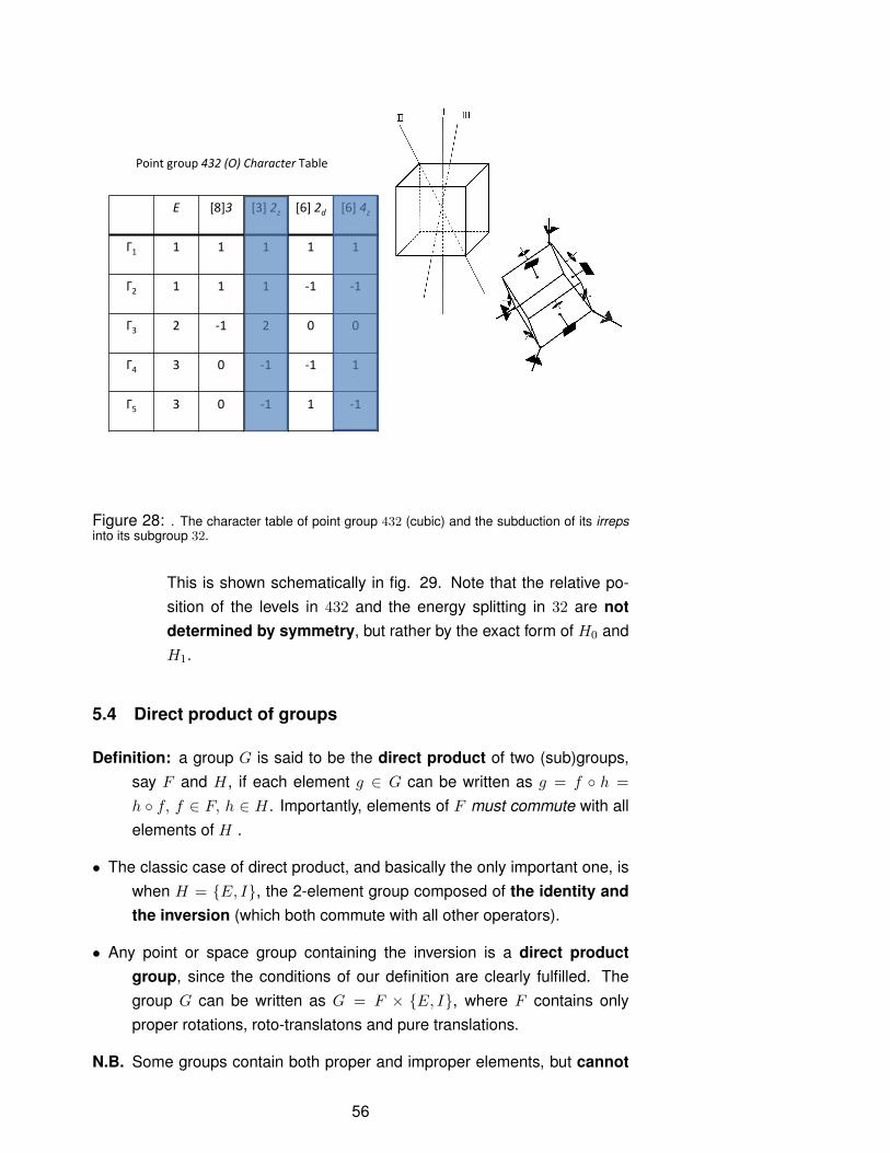
E [8]3 [3] 2z [6] 2d [6] 4z

Γ1 1 1 1 1 1

Γ2

1 1 1 -‐1 -‐1

Γ3

2 -‐1 2 0 0

Γ4

3 0 -‐1 -‐1 1

Γ5

3 0 -‐1 1 -‐1

Point group 432 (O) Character Table

Figure 28: . The character table of point group 432 (cubic) and the subduction of its irrepsinto its subgroup 32.

This is shown schematically in fig. 29. Note that the relative po-sition of the levels in 432 and the energy splitting in 32 are notdetermined by symmetry, but rather by the exact form of H0 andH1.

5.4 Direct product of groups

Definition: a group G is said to be the direct product of two (sub)groups,say F and H, if each element g ∈ G can be written as g = f ◦ h =

h ◦ f, f ∈ F, h ∈ H. Importantly, elements of F must commute with allelements of H .

• The classic case of direct product, and basically the only important one, iswhen H = {E, I}, the 2-element group composed of the identity andthe inversion (which both commute with all other operators).

• Any point or space group containing the inversion is a direct productgroup, since the conditions of our definition are clearly fulfilled. Thegroup G can be written as G = F × {E, I}, where F contains onlyproper rotations, roto-translatons and pure translations.

N.B. Some groups contain both proper and improper elements, but cannot

56

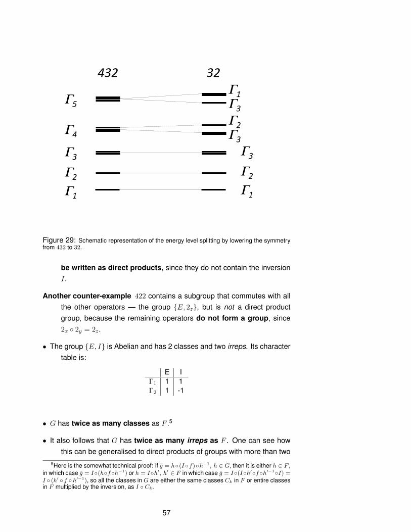
432 32

Γ1

Γ2

Γ3

Γ4

Γ5

Γ1

Γ2

Γ3

Γ3

Γ2

Γ3

Γ1

Figure 29: Schematic representation of the energy level splitting by lowering the symmetryfrom 432 to 32.

be written as direct products, since they do not contain the inversionI.

Another counter-example 422 contains a subgroup that commutes with allthe other operators — the group {E, 2z}, but is not a direct productgroup, because the remaining operators do not form a group, since2x ◦ 2y = 2z.

• The group {E, I} is Abelian and has 2 classes and two irreps. Its charactertable is:

E IΓ1 1 1Γ2 1 -1

• G has twice as many classes as F .5

• It also follows that G has twice as many irreps as F . One can see howthis can be generalised to direct products of groups with more than two

5Here is the somewhat technical proof: if g = h◦(I ◦f)◦h−1, h ∈ G, then it is either h ∈ F ,in which case g = I◦(h◦f◦h−1) or h = I◦h′, h′ ∈ F in which case g = I◦(I◦h′◦f◦h′−1◦I) =I ◦ (h′ ◦ f ◦h′−1), so all the classes in G are either the same classes Ck in F or entire classesin F multiplied by the inversion, as I ◦ Ck.

57

elements, and the importance of the commutation of all elements of Fwith all elements of H. In the general case, the number of classes in Gis the product of the classes in F times the classes in H.

• All the irreps of G = F × {E, I} can be obtained as follows:

� Start from the character table of F .

� Double the number of columns (classes). For each class Ck of Fcontaining the element f , there will be a new class I◦Ck containingthe element I ◦ f .

� For each Γi of F we get two irreps of G: Γig and Γiu.

� For the g- or gerade (even) irreps, we get:

χΓig(fCk = +χΓi(Ck)

χΓig(I ◦ Ck) = +χΓi(Ck) (81)

� For the g- or ungerade (odd) irreps, we get:

χΓiu(Ck) = +χΓi(Ck)

χΓiu(I ◦ Ck) = −χΓi(Ck) (82)

• This procedure is illustrated in the two tables here below. From the charac-ter table of F

E C1 C2 · · · CnΓ1 χ1(E) χ1(C1) χ1(C2) · · · χ1(Cn)Γ2 χ2(E) χ2(C1) χ2(C2) · · · χ2(Cn)... · · · · · · · · · · · · · · ·

Γn χn(E) χn(C1) χn(C2) · · · χn(Cn)

we obtain the character table of G:

E C1 C2 · · · Cn I I ◦ C1 I ◦ C2 · · · I ◦ CnΓ1g χ1(E) χ1(C1) χ1(C2) · · · χ1(Cn) +χ1(E) +χ1(C1) +χ1(C2) · · · +χ1(Cn)Γ2g χ2(E) χ2(C1) χ2(C2) · · · χ2(Cn) +χ2(E) +χ2(C1) +χ2(C2) · · · +χ2(Cn)

... · · · · · · · · · · · · · · · · · · · · · · · · · · · · · ·Γng χn(E) χn(C1) χn(C2) · · · χn(Cn) +χn(E) +χn(C1) +χn(C2) · · · +χn(Cn)

Γ1u χ1(E) χ1(C1) χ1(C2) · · · χ1(Cn) −χ1(E) −χ1(C1) −χ1(C2) · · · −χ1(Cn)Γ2u χ2(E) χ2(C1) χ2(C2) · · · χ2(Cn) −χ2(E) −χ2(C1) −χ2(C2) · · · −χ2(Cn)

... · · · · · · · · · · · · · · · · · · · · · · · · · · · · · ·Γnu χn(E) χn(C1) χn(C2) · · · χn(Cn) −χn(E) −χn(C1) −χn(C2) · · · −χn(Cn)

58

6 Lecture 6: Tensors and tensor products of repre-sentations

6.1 Tensor product of vector spaces

• Given two vector spaces V and W , one can define their tensor productV ⊗W , a new vector space, as the set of linear combination of orderedpairs of basis vectors of V and W . Essentially, one defines the basisvectors of V ⊗W as (ai|bj), ai ∈ V, bj ∈ W . The elements of V ⊗Ware linear combinations of (ai|bj). Clearly, the dimension of V ⊗W isdimV × dimW .

• The basis vectors of V ⊗W can be ordered in a single array as

[(a1|b1)(,a1|b2), · · · , (a1|bm), (a2|b1), · · · (an|bm)] (83)

• If the elements of V transform according to matrix A and those of W ac-cording to matrixB, then the elements of V ⊗W will transform accordingto the Kronecker product (or tensor product) A⊗B of the two matrices,where:

A⊗B =

a11B a12B · · · a1nB

a21B a22B · · · a2mB...

......

...an1B an2B · · · annB

(84)

The new matrix A⊗B has dimensions nm× nm.

• We can immediately see that the trace of A ⊗ B is the product of the twotraces: tr(A⊗B) = tr(A) tr(B).

6.2 Tensor product of representations

• Let’s assume that the elements of V transform according to a represen-tation Γ (reducible or irreducible) and the elements of W according toa representation ∆. Elements of the tensor product space V ⊗W willtransform according to representation Γ ⊗∆ — the tensor product ofthe two representations.

• The matrix representatives of Γ⊗∆ are the Kronecker product or matrixrepresentatives for Γ and ∆, as

59

DΓ⊗∆(g) = DΓ(g)⊗D∆(g) (85)

• A very important result on the characters of Γ⊗∆ follows immediately:

χΓ⊗∆(g) = χΓ(g)χ∆(g) (86)

Therefore, to determine the characters of a representation in thetensor product space, one simply multiplies the characters of therepresentations in the constituent spaces.

• This is an extremely important and powerful result: if we know the represen-tations of the constituent spaces, we can immediately find the charac-ters of the tensor product representation and decompose it into irreps.This can be repeated many times, giving rise to representations anddecomposition of extremely complex tensor spaces with very little work.

6.3 * Extended example: vibrational spectra of planar moleculeswith symmetry Dn

• We have already seen examples for D3 (32, section 5.2, page 50) and forD4(422, section 4.3, page 43). Armed with the knowledge of tensorproduct, we can now solve the problem for any n.

• We can consider the space of the modes as the tensor product of twospaces: V is the space of scalar functions on the regular polygon with nsides, and W is the space of ordinary vectors in 2D. The basis functionsof V can be taken as arrays of n numbers, all of them 0 except for a 1

corresponding to one of the vertices. The space of ordinary vectors hasits usual basis functions (e.g.,i, j). For example, the top-left mode inblock A of fig. 20 can be written in tensor notation as ([1, 0, 0, 0]|i).

• Let us consider independently the representations ofDn onto the two spacesV and W — call them Γ and ∆ as before.

• Γ is the so-called permutational representation, although Dn is not ingeneral the full permutation group of the n-polygon. We can deduce itscharacters as follows:

� The character of the identity E is n

� Cn ( the group of pure rotations around z) is a subgroup of Dn. Theelements of Cn will generate several classes in Dn — for exam-ple, we know that in D4 there are two classes of this kind, 2z and

60

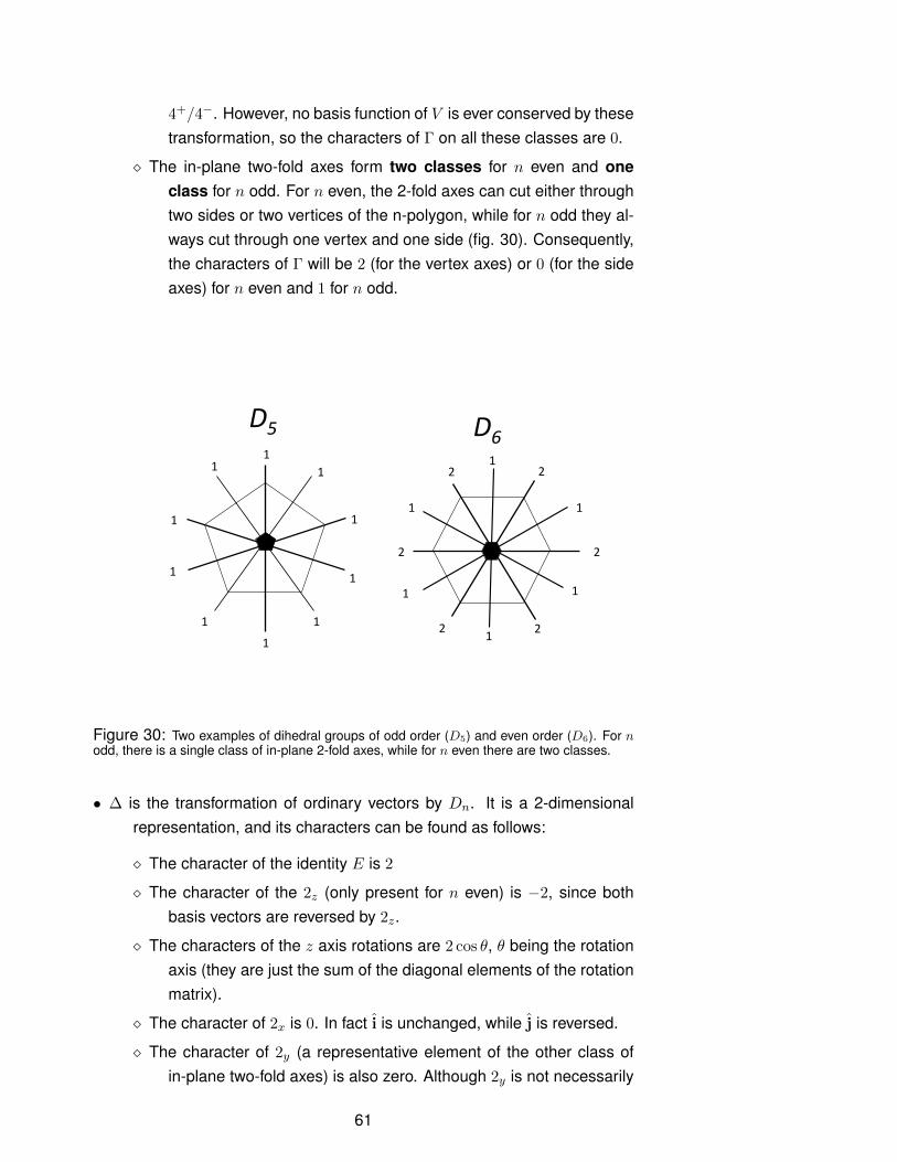
4+/4−. However, no basis function of V is ever conserved by thesetransformation, so the characters of Γ on all these classes are 0.

� The in-plane two-fold axes form two classes for n even and oneclass for n odd. For n even, the 2-fold axes can cut either throughtwo sides or two vertices of the n-polygon, while for n odd they al-ways cut through one vertex and one side (fig. 30). Consequently,the characters of Γ will be 2 (for the vertex axes) or 0 (for the sideaxes) for n even and 1 for n odd.

2

2 2

2

2 2

1

1

1

1

1

1

1 1 1

1

1

1

1

1

1

1

D5 D6

Figure 30: Two examples of dihedral groups of odd order (D5) and even order (D6). For nodd, there is a single class of in-plane 2-fold axes, while for n even there are two classes.

• ∆ is the transformation of ordinary vectors by Dn. It is a 2-dimensionalrepresentation, and its characters can be found as follows:

� The character of the identity E is 2

� The character of the 2z (only present for n even) is −2, since bothbasis vectors are reversed by 2z.

� The characters of the z axis rotations are 2 cos θ, θ being the rotationaxis (they are just the sum of the diagonal elements of the rotationmatrix).

� The character of 2x is 0. In fact i is unchanged, while j is reversed.

� The character of 2y (a representative element of the other class ofin-plane two-fold axes) is also zero. Although 2y is not necessarily

61

perpendicular to 2x (e.g., in the case of n = 8), its matrix repre-sentative is still related by a similarity transformation to the matrixrepresentative of 2x, the the characters remain the same.

• We can also easily add a central atom. Its modes represent an additionalsubspace and transform like ∆, so its characters are simply added tothe tensor product characters. This can be summarised as follows: forn even

E 2z 2C1z 2C2

z · · · (n/2)2x (n/2)2yχΓ n 0 0 0 · · · 2 0χ∆ 2 −2 2 cos θ 2 cos 2θ · · · 0 0

χΓ⊗∆ 2n 0 0 0 · · · 0 0χΓ⊗∆+∆ 2n+ 2 −2 2 cos θ 2 cos 2θ · · · 0 0

for n odd

E 2C1z 2C2

z · · · n2xχΓ n 0 0 · · · 1χ∆ 2 2 cos θ 2 cos 2θ · · · 0

χΓ⊗∆ 2n 0 0 · · · 0χΓ⊗∆+∆ 2n+ 2 2 cos θ 2 cos 2θ · · · 0

• We can see that our result is in agreement with our previous findings for D3

(eq. 48 page 36) and D4 (page 44).

• Let us try with D6 (622). The irrep character table is in fig. 27. The charac-ters are:

E 2z 2 6z 2 3z 3 2x 3 2yχΓ⊗∆ 12 0 0 0 0 0χΓ⊗∆+∆ 14 −2 1 −1 0 0

By applying eq. 45 we obtain:

Γ⊗∆ = Γ1 + Γ2 + Γ3 + Γ4 + 2Γ5 + 2Γ6

Γ⊗∆ + ∆ = Γ1 + Γ2 + Γ3 + Γ4 + 3Γ5 + 2Γ6 (87)

• The central atom modes clearly transform as Γ5 (≡ ∆, characters 2| −2|1| − 1), and so will the pure translations of the whole molecule (whichare also ordinary vectors). One of the 1-dim modes must correspond toa pure rotation of the molecule. It is easy to see that this must be Γ2,since this mode must be invariant by all z-axis rotations. Therefore theset of non-zero-frequency normal modes is:

Γ⊗∆− Γ2 − Γ5 = Γ1 + Γ3 + Γ4 + Γ5 + 2Γ6

Γ⊗∆ + ∆− Γ2 − Γ5 = Γ1 + Γ3 + Γ4 + 2Γ5 + 2Γ6 (88)

62

three singlets and three doublets or three singlets and four doubletswithout or with the central atom, respectively.

• Γ1 is the only Raman-active mode (in 2D, the 2-fold axis corresponds to theinversion in 3D). All other modes are IR-active. in a molecular crystal,Γ2 will give rise to Raman-active phonon modes.

6.4 “Ordinary” tensors

• What we have just introduced is a rather abstract definition of tensors, andwe have applied it to vector spaces that do not look anything like themore familiar tensors in physics.

• “Ordinary” tensors are actually closely related to the ones we just intro-duced. They are tensor products of spaces or ordinary (polar) vec-tors or axial vectors.

• In free space, ordinary polar vectors and axial vectors transform in thesame way under proper rotations, i.e., according to a 3-dimensional ir-reducible representation of the continuous group of proper rotations. Ifone includes improper rotations, polar vectors, forming a space that wewill call V , transform as an ungerade irreducible representation of thecontinuous group of proper and improper rotations, which we shall callΓu. Axial vectors, forming a space A, transform under the correspond-ing gerade irrep Γg.

• We define polar tensors and axial tensors of different ranks as follows:

Rank 0 1 2 3 4 · · ·Polar tensors — space scalars V V ⊗ V = V 2 V 3 V 4 · · ·

Polar tensors — representation Γ1g Γu Γu ⊗ Γu =[Γ2u

]g

[Γ3u

]u

[Γ4u

]g

· · ·Axial tensors — space pseudo-scalars A A⊗ V A3 A3 ⊗ V · · ·

Axial tensors — representation Γ1u Γg [Γg ⊗ Γu]u[Γ3g

]g

[Γ3g ⊗ Γv

]u· · ·

� The tensor product representation is gerade if it contains an evennumber of Γu, ungerade otherwise. We have indicated this as []gor []u

� There are many different combinations of spaces that give the sametransformation rules, and are therefore isomorphic (symbol∼=). Forexample, A⊗A ∼= V ⊗ V and A3 ∼= V 2 ⊗A.

� We have also introduced the rank-zero tensors, known as scalarsand pseudo-scalars. They transform like the totally symmetricalrepresentation of the proper rotation group SO(3), but are geradeand ungerade, respectively.

63

• Polar tensors of odd rank are parity-odd. Polar tensors of even rankare parity even.

• Axial tensors of odd rank are parity-even. Axial tensors of even rankare parity odd.

Example of polar tensor: The permittivity tensor is a rank-2 polar tensor,defined by the formula:

Di = εijEj (89)

Example of axial tensor: The linear magneto electric tensor is a rank-2axial tensor, defined by the formula:

Pi = µijBj (90)

in fact, the electrical polarisation Pi an ordinary vector, whereas themagnetic field Bj is an axial vector.

6.5 “Materials” tensors vs. “Field” tensors

• A distinction can be made between tensors that describe intrinsic proper-ties or spontaneous effects of the crystals — so-called materials ten-sors, and tensors that describe external forces or the reaction of thematerials to those forces — so-called field tensors.

Materials tensors representing macroscopic properties must have the fullpoint-group symmetry of the crystal. This is another way to statethe famous Neumann’s principle: “The symmetry elements of any phys-ical property of a crystal must include the symmetry elements of thepoint group of the crystal”. It is applicable to any physical observablemeasured with a probe that is insensitive to lattice periodicity. In thelanguage of irreps, materials tensors must transform like the totallysymmetric irrep of the crystal class: Γ1 or Γ1g for acentric and cen-tric classes, respectively. Examples of materials tensors are: per-mittivity tensor, permeability tensor, conductivity tensor, piezoelectric-ity tensor, magneto-electricity tensor, spontaneous strain tensor, elastictensor.

Field tensors can have any symmetry — in fact they usually define they ownsymmetry. For example, the applied electric field (an ordinary polar vec-tor) will have a continuous rotational symmetry around its own direction

64

and it is clearly parity-odd (ungerade). However, there can be otherrestrictions on the elements of a field tensor (see here below). Exam-ples of field tensors, in addition to the usual fields, are: stress tensor,induced strain tensor.

Example: Hooke’s law in materials In tensor form, Hooke’s law of elasticityis expressed as:

σij = cijklεkl (91)

or its converse

εij = sijklσkl (92)

� σij is the applied stress tensor — a field tensor

� εkl is the induced strain tensor — a field tensor

� cijkl and sijkl are the stiffness tensor and the elastic tensor, re-spectively —both materials tensors. They are doubly symmetrictensors in ij and kl separately, so they have 36 elements (seehere below for an explanation).

6.6 Internal symmetry of tensor elements

• In addition to the crystal symmetry properties of materials tensors, whichwe just described, many tensors are symmetric by exchange of someof their indices (as hinted here above).

• Some tensors reflect equilibrium properties of the crystal, for exampleunder an applied external field, and can be obtained by differentiationof the free energy. If the differentiation occurs twice with respect to thesame quantity, the tensor is symmetric.

Example: Permittivity tensor:

Pi = − ∂F∂Ei

εij = − ∂2F

∂Ei∂Ej(93)

so the permittivity tensor is clearly symmetric by exchange of its indices.

65

Counter-example: Magnetoelectric tensor:

Pi = µijBj

µij = − ∂2F

∂Ei∂Bj(94)

so the magneto electric tensor is not a symmetric tensor.

• Some field tensors are symmetric by construction – for example, the stresstensor σij is symmetric because it excludes any torque component. Asa consequence, the piezoelectric tensor diαβ, defined as

Pi = diαβσαβ (95)

is symmetric in αβ (but the symmetry does not involve the first index i).

• Some materials tensor describing non-equilibrium steady-state properties,such as the conductivity tensor, are also symmetric. The symmetryproperties of such tensors are expressed by the so-called Onsager reci-procity principle (see book by J.F. Nye).

6.7 Symmetrised and anti-symmetrised tensor spaces

• As we had just seen, certain tensors are symmetric by exchange of oneor more pairs of indices. It is also useful in some cases to considerantisymmetric tensors by exchange of indices. When one considersthe tensor product of a vector space by itself, V ⊗ V , one can see howthe definition of symmetric and antisymmetric tensors naturally arises.If the basis vectors of V ⊗ V (with dimension n2) are:

[(a1|a1)(,a1|a2), · · · , (a1|an), (a2|a1), · · · (an|an)] (96)

then one can consider two subspaces of V ⊗ V : the symmetric sub-space [V ⊗ V ], with dimension 1

2n(n+ 1) and basis vectors:

[(a1|a1),

1

2(a1|a2) +

1

2(a2|a1), · · · , 1

2(a1|an) +

1

2(an|a1), · · · , (an|an)

](97)

and the the anti-symmetric subspace {V ⊗ V }, with with dimension12n(n− 1) and basis vectors:

66

[(1

2(a1|a2)− 1

2(a2|a1), · · · , 1

2(a1|an)− 1

2(an|a1), · · · , 1

2(an−1|an)− 1

2(an|an−1)

](98)

• There is a very useful formula for the characters of the symmetric andantisymmetric subspaces, which we present without proof:

χ[Γ⊗Γ](g) =1

2

[χ2

Γ(g) + χΓ(g2)]

χ{Γ⊗Γ}(g) =1

2

[χ2

Γ(g)− χΓ(g2)]

(99)

where g2 = g ◦ g.

• This rule enables us to construct the transformation properties of very com-plex tensors. For example, the doubly symmetric elastic tensor sijkltransforms like the doubly symmetric tensor representation [Γ⊗ Γ] ⊗[Γ⊗ Γ], and its characters are easily determined from eq. 99, if oneknows the characters of Γ.

• Note that many relevant decompositions of tensor representations can befound on the Bilbao Crystallographic Server http://www.cryst.ehu.es/rep/point.html.

Example: transformation properties of the piezoelectric tensor in the point group 32.The definition of the piezoelectric tensor diαβ is in eq. 95. It is a 3rd-rankpolar tensor that is symmetric in the last two indices, so it transformsaccording to representation Γ⊗ [Γ⊗ Γ]. Γ is the ordinary vectors trans-formation by 32. As we already know, Γ = Γ2 + Γ3. The character tablefor Γ is therefore:

E 2A 3K3 0 -1

Let’s employ eq. 99 to determine the characters of [Γ⊗ Γ]. For theidentity and the 2-fold axes, g2 = E, whereas for the 3-fold rotationsA2 = B. Therefore:

χ[Γ⊗Γ](E) =1

2

[χ2

Γ(E) + χΓ(E2)]

= 6

χ[Γ⊗Γ](A) =1

2

[χ2

Γ(A) + χΓ(A2)]

= 0

χ[Γ⊗Γ](K) =1

2

[χ2

Γ(K) + χΓ(K2)]

= 2 (100)

67

Therefore [Γ⊗ Γ] = 2Γ1 + 2Γ3. Multiplying by Γ again we obtain thecharacter table for Γ⊗ [Γ⊗ Γ]:

E 2A 3K18 0 -2

This decomposes into Γ ⊗ [Γ⊗ Γ] = 2Γ1 + 4Γ2 + 6Γ3. However, thepiezoelectric tensor is a materials property tensor, and it has thereforeto transform according to the totally symmetric irrep Γ1. All the othercomponents must correspond to zero elements of the tensor matrix. Γ1

appears twice in the decomposition. Therefore, the matrix elements ofdiαβ are described by only two independent parameters.

6.8 Matrix transformations of tensors

• Up to this point, we have employed the powerful machinery of representa-tion theory to describe the transformation properties of tensors. How-ever, in order to perform calculations, we need the actual matrix formof the tensors, which of course depends on the choice of coordinates,Cartesian, spherical and crystallographic being possible choices. Also,we need another explicit form of transformation rules, since the Kro-necker form is not of practical application.

• The matrix form of the tensor arises from writing the elements of a tensorspace as

T =∑i,j,k,···

Ti,j,k,··· (ai|bj |ck| · · · ) (101)

where ai,bj , c etc. are basis sets for ordinary vectors. With this nota-tion:

O(g)T =∑

l,m,n,···Tl,m,n,···

∑i,j,k,···

Rli(g)aiRmj(g)bjRnk(g)ck · · ·

=∑i,j,k,···

∑l,m,n,···

Tl,m,n,···Rli(g)Rmj(g)Rnk(g)

(ai|bj |ck| · · · )

(102)

where the Rli(g) are the ordinary proper rotation matrices, i.e., the ma-trix representative of the group elements on the space of ordinary vec-tors. In the case of improper rotations, one has to take into account

68

whether the tensor is polar or axial. This can be summarised in thefollowing formula, where p(g) is the parity of g:

O(g)Tijk··· =∑

l,m,n,···Tl,m,n,···Rli(g)Rmj(g)Rnk(g) · · · (polar tensors)

O(g)Tijk··· = (−1)p(g)∑

l,m,n,···Tl,m,n,···Rli(g)Rmj(g)Rnk(g) · · · (axial tensors)

(103)

6.9 Allowed physical properties and materials tensors elements

• Two central questions about physical properties described by materials ten-sors are:

1. which physical properties are allowed in certain crystal sym-metries, and how many independent parameters are neededto describe them?

2. what is the explicit form of the tensors in a given coordinatesystem?

these questions can be answered exclusively by use of symmetry argu-ments.

• The first question can be fully addressed by employing character decompo-sition, as we have seen in the piezoelectricity tensor example on page67. One determines the characters of the tensor representation (inthat case Γ ⊗ [Γ⊗ Γ]), decomposes the resulting character table intoirreps and considers the number of times Γ1 or (Γ1g for centrosymmet-ric groups) appears in the decomposition.

� If Γ1 appears 0 times, then the physical properties described by thistensor is forbidden in that particular symmetry group.

� If Γ1 appears n > 0 times, then the physical properties described bythis tensor are spanned by n independent parameters in that par-ticular symmetry group, meaning that the variability of that proper-ties in all molecules or crystals with that symmetry is described byn parameters.

• From the parity classification of polar and axial tensors (page 63), it followsimmediately that physical properties described by polar tensors ofodd rank and axial tensors of even rank cannot exist in systems

69

having centrosymmetric symmetry groups. In fact, Γ1g can neverappear in the decomposition of an ungerade representation.

• Therefore, for example, piezoelectricity and ferroelectricity are only restrictedto non-centrosymmetric groups.

• Further restrictions can be found by actually applying the decompositionformula. For example, ferroelectricity and pyroelectricity are restricted toonly 10 point groups (out of the 21 non-centrosymmetric point groups):1, 2, m, 2mm, 4, 4mm, 3, 3m, 6 and 6mm. Every non-centrosymmetricpoint group is piezoelectric, except 432.

• To find the explicit form of the tensors in a given coordinate system, onecan employ the projector operators. One simply takes non-symmetry-specific form of the tensor, with appropriately symmetrised indices ifnecessary, and projects it onto the totally symmetric representation Γ1:

Tijk =1

h

∑g

∑lmn

TlmnRli(g)Rmj(g)Rnk(g) (104)

where, again, one can see that the symmetrised tensor will be zero forparity-odd tensors in centro-symmetric groups.

6.10 *Example: explicit form of the piezoelectric tensor in 32.

• Following on from the previous example, we will now determine the ex-plicit form of this tensor in Cartesian coordinates. The non-symmetry-specific tensor has 18 independent components, and the transforma-tion matrices are in eq. 16. The form in 3D is obtained by settingR31 = R32 = R13 = R23 = 0. R33 = 1 for E, A, and B and −1 for K, Land M . We will use the projection formula:

diµν =1

h

∑g

∑lκλ

dlκλRli(g)Rκµ(g)Rλν(g) (105)

where we use the Greek letter to label the symmetric indices.

� We start by calculating 1/h∑

g over the 6 elements of the group for allthe different combinations of matrices, which we will indicate withthe notation:

(11)(12)(33) =1

6

∑g

R11(g)R12(g)R33(g) (106)

70

the order of the matrices clearly does not matter. This calculationis further simplified by the fact that all matrix elements containinga “3” (13, 23, 31, 32) are zero except for 33. We can find all thenon-zero elements with the help of a spreadsheet:

(11)(22)(33) = (11)(33)(22) = (22)(11)(33) =1

2

(22)(33)(11) = (33)(11)(22) = (33)(22)(11) =1

2

(12)(21)(33) = (12)(33)(21) = (21)(12)(33) = −1

2

(21)(33)(12) = (33)(12)(21) = (33)(21)(12) = −1

2

(11)(11)(22) = (11)(22)(11) = (22)(11)(11) =1

4

(11)(12)(21) = (11)(21)(12) = (12)(11)(21)1

4

(21)(11)(12) = (12)(21)(11) = (21)(12)(11) =1

4

(22)(22)(22) =1

4

(12)(12)(22) = (12)(22)(12) = (22)(12)(12) = −1

4

(21)(21)(22) = (21)(22)(21) = (22)(21)(21) = −1

4(107)

� We now consider the summation∑

lκλ in (eq. 105). One can no-tice that the second index in each rotation matrix (the one weunderlined) determines which symmetrised tensor element thatmatrix will contribute to, so, for example in our notation, the term(21)(12)(33) will provide a contribution −1

2d213 to d123. With a bit ofbookkeeping, one gets the following:

d123 = d132 = A

d213 = d213 = −A

d112 = d121 = d211 = B

d222 = −B (108)

where

A =1

2[d123 − d213]

B =1

4[2d112 + d211 − d222] (109)

71

All the other elements of the tensor are zero.

As we had predicted using irrep analysis, the piezoelectric tensor has 2free parameters in 32 (A and B), corresponding to the number of timesΓ1 is contained in Γ⊗ [Γ⊗ Γ].

72

Symmetry in Condensed Matter Physics - University of · PDF fileSymmetry in Condensed Matter...

Documents

Transcript of Symmetry in Condensed Matter Physics - University of · PDF fileSymmetry in Condensed Matter...