SYMMETRIES IN CLASSICAL FIELD THEORY

September 27, 2004 22:27 WSPC/IJGMMP-J043 00029

International Journal of Geometric Methods in Modern PhysicsVol. 1, No. 5 (2004) 651–710c© World Scientific Publishing Company

SYMMETRIES IN CLASSICAL FIELD THEORY

MANUEL DE LEON∗, DAVID MARTIN DE DIEGO† andAITOR SANTAMARIA-MERINO‡

Departamento de MatematicasInstituto de Matematicas y Fısica FundamentalConsejo Superior de Investigaciones Cientıficas

Serrano 123, 28006 Madrid, Spain∗[email protected]†[email protected]‡[email protected]

Received 6 April 2004Accepted 21 June 2004

The multisymplectic description of Classical Field Theories is revisited, including itsrelation with the presymplectic formalism on the space of Cauchy data. Both descriptionsallow us to give a complete scheme of classification of infinitesimal symmetries, and toobtain the corresponding conservation laws.

Keywords: Symmetry; multisymplectic form; classical field theory; Cauchy surface.

1. Introduction

The multisymplectic description of Classical Field Theories goes back to the endof the sixties, when it was developed by the Polish school headed by W. Tulczyjew(see [3, 36–38, 68]), and also independently by P. L. Garcıa-Perez and A. Perez-Rendon [20–22], and H. Goldschmidt and S. Sternberg [25]. From that time, thistopic has continuously received a lot of attention mainly after the paper [7], andmore recently in [19, 33, 34, 61, 62]. A serious attempt to get a full developmentof the theory has been done in the monographs [28, 29] (see also [54] for higher-order theories). In addition, the multisymplectic setting is proving to be useful fornumerical purposes [56].

The final goal is to obtain a geometric description similar to the symplectic onefor Lagrangian and Hamiltonian mechanics. Therefore, the first idea was to intro-duce a generalization of the symplectic form. The canonical symplectic structureon the cotangent bundle of a configuration manifold is now replaced by multisym-plectic forms canonically defined on the bundles of exterior forms on the bundleconfiguration π: Y → X of the theory in consideration. These geometric structurescan be abstracted to arbitrary manifolds; its study constitutes a new subject of

651

Int.

J. G

eom

. Met

hods

Mod

. Phy

s. 2

004.

01:6

51-7

10. D

ownl

oade

d fr

om w

ww

.wor

ldsc

ient

ific

.com

by B

AY

LO

R U

NIV

ER

SIT

Y o

n 06

/24/

14. F

or p

erso

nal u

se o

nly.


652 M. de Leon, D. Martın de Diego & A. Santamarıa-Merino

interest for geometers [5, 6, 52, 57, 58] which could give new insights as did happenwith symplectic geometry in the sixties.

On the other hand, if we start with a Lagrangian density, we can first constructa Lagrangian form from a volume form fixed on the space-time manifold X , andthen, using the bundle structure of the 1-jet prolongation πXZ : Z → X of Y , weconstruct a multisymplectic form on Z (provided that the Lagrangian is regular).

In this geometric context, one can present the field equations in two alternativeways: in terms of multivectors (see [11–19]), or in terms of Ehresmann connections[44, 48, 49, 52].

Let us remark that there are alternative approaches using the so-called polysym-plectic structures (see [23, 24, 35, 63–65]) or even n-symplectic structures (see [53]for a recent survey). Here, we shall present the field equations in terms of Ehresmannconnections; indeed, note that in Lagrangian or Hamiltonian mechanics one looksfor curves, or, in an infinitesimal version, tangent vectors; now, we look for sectionsof the corresponding bundles, which infinitesimally correspond to the horizontalsubspaces of Ehresmann connections. In fact, the Euler–Lagrange equations (moregenerally, the de Donder equations) and Hamilton equations can be described in aform which is very similar to the corresponding ones in Mechanics. Both formalisms(Lagrangian and Hamiltonian) are related via the Legendre transformation. Thecase of singular theories is also considered, and a constraint algorithm is obtained.

According with these different descriptions, we have different notions of infinites-imal symmetries (see [60] for a description based on the calculus of variations). Theaim of the present paper is to classify the different kinds of infinitesimal symmetriesand to study their relationship with conservation laws in the geometric context ofmultisymplectic geometry and Ehresmann connections.

In addition, by choosing a Cauchy surface, we also develop the correspondinginfinite dimensional setting in the space of Cauchy data. Both descriptions arerelated by means of integration along the Cauchy surfaces, allowing to relate theabove symmetries with the ones of the presymplectic infinite dimensional system.

Let us remark that we consider boundary conditions throughout the paper.The paper is structured as follows. Section 2 describes the Lagrangian setting

for the Classical Field Theories of first order using the tools of jet manifolds, in bothregular and singular cases. Multisymplectic forms and brackets are introduced at theend of the section in order to be used later. Section 3 is devoted to give a Hamilto-nian description for Classical Field Theories, including the Legendre transformationand the equivalence theorem. The singular case is also discussed. Section 4 dealswith the theory of Cauchy surfaces for the Classical Field Theory, where the toolsthat will be required later are introduced. In particular, the integration method, asa way to connect the finite dimensional setting and the theory of Cauchy Surfaces,is discussed in depth. The singular case and the Poisson brackets are also con-sidered. Section 5 thoroughly describes the different infinitesimal symmetries forthe Lagrangian and Hamiltonian settings, using the tools that have been describedin the previous sections. In Sec. 6, we discuss the Momentum Map in the finite

Int.

J. G

eom

. Met

hods

Mod

. Phy

s. 2

004.

01:6

51-7

10. D

ownl

oade

d fr

om w

ww

.wor

ldsc

ient

ific

.com

by B

AY

LO

R U

NIV

ER

SIT

Y o

n 06

/24/

14. F

or p

erso

nal u

se o

nly.


Symmetries in Classical Field Theory 653

and infinite dimensional settings. The paper finishes with Sec. 7, in which we illus-trate the concepts discussed with the examples of the Bosonic string, following thePolyakov approach, and the Klein–Gordon field.

Throughout this paper, we shall use the following notations: X(M) will denotethe Lie algebra of vector fields on a manifold M , and £X will be the Lie deriva-tive with respect to a vector field X . The differential of a differentiable mappingF : M → N will be indistinctly denoted by F∗, dF or TF. By C∞(M) we denotethe algebra of smooth functions on a manifold M .

2. Lagrangian Formalism

2.1. The setting for classical field theories

Consider a fibration π = πXY : Y → X , where Y is an (n + 1 + m)-dimensionalmanifold and X is an orientable (n + 1)-dimensional manifold. We shall also fixa volume form on X , which will be denoted by η. We can choose fibered coordi-nates (xµ, yi) in Y , so that π(xµ, yi) = (xµ), and assume that the volume form isη = dn+1x = dx0 ∧ · · · ∧ dxn. Here, 0 ≤ µ, ν, . . . ≤ n and 1 ≤ i, j, . . . ≤ m.

Remark 2.1. Time dependent mechanics can be considered as an example of clas-sical field theory, where X is chosen to be the real line R, representing time, andthe fiber over t represents the configuration space at time t.

We shall also use the following notation:

dnxµ := ι∂/∂xµdn+1x, dn−1xµν:= ι∂/∂xµι∂/∂xν dn+1x, . . . .

The first-order jet prolongation J1π is the manifold of classes j1xφ of sections φ of π

around a point x of X which have the same Taylor expansion up to order one. J1π

can be viewed as the generalization of the phase space of the velocities for classicalmechanics. Therefore, J1π, which we shall denote by Z, is an (n+1+m+(n+1)m)-dimensional manifold. We also define the canonical projections πXZ : Z → X byπXZ (j1

xφ) = x, and πYZ : Z → Y by πYZ (j1xφ) = φ(x) (see Fig. 1). We shall also use

the same notation η for the pullback of the chosen volume form η on X to Z alongthe projection. If we have adapted coordinates (xµ, yi) in Y , then we can defineinduced coordinates in Z, given by (xµ, yi, zi

µ), such that

xµ(j1xφ) = xµ(x)

yi(j1xφ) = yi(φ(x)) = φi(x)

ziµ(j1

xφ) =∂φi

∂xµ

∣∣∣∣x

.

As usual, one can define the concept of verticality, by defining the followingsubbundles:

Vyπ := (Tyπ)−1(0x)

VzπXZ := (TzπXZ )−1(0x).

Int.

J. G

eom

. Met

hods

Mod

. Phy

s. 2

004.

01:6

51-7

10. D

ownl

oade

d fr

om w

ww

.wor

ldsc

ient

ific

.com

by B

AY

LO

R U

NIV

ER

SIT

Y o

n 06

/24/

14. F

or p

erso

nal u

se o

nly.



Z = J1πXY

Y

X

πYZ

πXZ

πXY

φ

j1φ

(xµ, yi, ziµ)

(xµ, yi)

(xµ)

8><>:

dim X = n + 1

dim Y = n + 1 + m

dim Z = n + 1 + m + (n + 1)m

Fig. 1.

We can consider the more general case in which X is a manifold with boundary ∂X ,and we also have boundaries for manifolds Y and Z, given by ∂Y = π−1(∂X) and∂Z = π−1

XZ (∂X), respectively. A boundary condition is encoded in a subbundle B of∂Z → ∂X , and restricting ourselves to sections φ: X → Y such that j1φ(∂X) ⊆ B

(see [3]).There are several other alternative (and equivalent) definitions of the first-

order jet bundle, such as considering the affine bundle over Y whose fiber overy ∈ π−1(x) consists of linear sections of TπXY , modeled over the vector bundle onY whose fiber over y ∈ π−1(x) is the space of linear maps of TxX to Vyπ; in otherwords, Z is an affine bundle over Y modeled on the vector bundle π∗T ∗X ⊗Y Vπ

(see [28, 66, 67]).The first-order jet bundle is equipped with a geometric object Sη, which depends

on our choice of the volume form, called vertical endomorphism (see [9] or [67]).What follows is an alternative way to define it. First of all, we construct theisomorphism (vertical lift)

v: π∗T ∗X ⊗Y Vπ → VπYZ

as follows: given f ∈ (π∗T ∗X⊗Y Vπ)|j1φ consider the curve γf : R → π−1YZ (πYZ (j1

xφ))given by

γf (t) = j1xφ + tf,

Int.

J. G

eom

. Met

hods

Mod

. Phy

s. 2

004.

01:6

51-7

10. D

ownl

oade

d fr

om w

ww

.wor

ldsc

ient

ific

.com

by B

AY

LO

R U

NIV

ER

SIT

Y o

n 06

/24/

14. F

or p

erso

nal u

se o

nly.



for all t ∈ R. Now define

fv =d

dtγf (t)∣∣∣∣t=0

.

If (xµ, yi) are fibered coordinates on Y and f = f iµdxµ|x ⊗ ∂

∂yi

∣∣φ(x)

then

fv = f iµ

∂

∂ziµ

∣∣∣∣j1xφ

.

Let x be a point of X and φ ∈ Γx(π), where Γx(π) denotes the set of all localsections around the point x. If V0, . . . , Vn are n + 1 tangent vectors to J1π at thepoint j1

xφ ∈ Z, then we have that Tj1xφπYZ (Vµ) − Txφ Tj1

xφπXZ (Vµ) ∈ (Vπ)φ(x)

(this is the vertical differential of a vector field on Z). From the volume form η, wealso construct a family of 1-forms ηµ as follows:

ηµ(x) = (−1)n+1−µiTj1xφπXZ (V0) · · · iTj1xφπXZ (Vµ) · · · iTj1xφπXZ (Vn) η(x),

where the hat over a term means that it is omitted.Next, we define the vertical endomorphism Sη as follows:

(Sη)j1xφ(V0, . . . , Vn) =

n∑i=0

(ηi(x) ⊗ (Tj1xφπYZ (Vi) − Txφ Tj1xφπXZ (Vi)))v .

Whenever we pick a different volume form Fη, then (Fη)µ = Fηµ, whence we alsoget SFη = FSη, where F : X → R is a nowhere-vanishing smooth function on X .

The vertical endomorphism can be also written in local induced coordinates asfollows

Sη = (dyi − ziµdxµ) ∧ dnxν ⊗ ∂

∂ziν

.

Higher-order jet bundles can be defined in a similar manner. The second-order jetbundle, for example, is an

(n + 1 + m + (n + 1)m +

(n+2

2

)m)-dimensional manifold,

which has induced coordinates (xµ, yi, ziµ, zi

µν), where

ziµν(j1

pφ) =∂2φi

∂xµ∂xν

∣∣∣∣p

.

These bundles allow us to define the total derivative associated with the partialderivative vector fields, which are locally expressed as

d

dxµ=

∂

∂xµ+ zi

µ

∂

∂yi+ zi

µν

∂

∂ziν

+ · · · .

2.2. Jet prolongation of vector fields

Definition 2.2. A 1-form θ ∈ Λ1(Z) is said to be a contact 1-form whenever

(j1φ)∗θ = 0

for every section φ of π.

Int.

J. G

eom

. Met

hods

Mod

. Phy

s. 2

004.

01:6

51-7

10. D

ownl

oade

d fr

om w

ww

.wor

ldsc

ient

ific

.com

by B

AY

LO

R U

NIV

ER

SIT

Y o

n 06

/24/

14. F

or p

erso

nal u

se o

nly.



If (xµ, yi, ziµ) is a system of local coordinates on Z, then the contact forms are

locally spanned by the 1-forms

θi = dyi − ziµdxµ.

We shall denote by C the algebraic ideal of the contact forms, and by I(C)the differential ideal generated by the contact forms, i.e., the ideal of the exterioralgebra generated by the contact forms and their differentials.

The distribution determined by the annihilation of the contact forms on Z iscalled the Cartan distribution and it plays a fundamental role, since it is thegeometrical structure which distinguishes the holonomic sections (sections which areprolongations of sections of πXY ) from arbitrary sections of πXZ (see [4, 39–42,59]for more details).

Lemma 2.3. For any vector field X in Z, the following two conditions areequivalent:

(i) For every Y in the Cartan distribution £XY lies in the Cartan distribution;i.e., X preserves the Cartan distribution.

(ii) X preserves C, i.e., for every θ ∈ C,£Xθ ∈ C.

If any of the preceding two holds, then X preserves I(C), i.e., for everyα ∈ I(C),£Xα ∈ I(C).

Definition 2.4. Given a vector field ξY ∈ X(Y ), then its 1-jet prolongation isdefined as the unique vector field ξ

(1)Y ∈ X(Z) projectable onto ξY by πYZ , and

which preserves the Cartan distribution (i.e., £ξ(1)Y

θ ∈ C for every contact form θ).

If ξY is locally expressed as

ξY = ξµY

∂

∂xµ+ ξi

Y

∂

∂yi,

then the 1-jet prolongation of ξY must have the following form

ξ(1)Y = ξµ

Y

∂

∂xµ+ ξi

Y

∂

∂yi+(

dξiY

dxµ− zi

ν

dξνY

dxµ

)∂

∂ziµ

. (2.1)

Assume that the local expression of ξ(1)Y is

ξ(1)Y = ξµ

Y

∂

∂xµ+ ξi

Y

∂

∂yi+ ξi

µY

∂

∂ziµ

. (2.2)

In order to see that (2.2) has the form (2.1), pick i ∈ 1, 2, . . . , m, and impose thesecond condition £

ξ(1)Y

θi ∈ C. We have

£ξ(1)Y

θi =∂ξi

Y

∂xµdxµ +

∂ξiY

∂yjdyj − ξi

µY dxµ − ziµ

(∂ξµ

Y

∂xνdxν +

∂ξµY

∂yjdyj

)=(

∂ξiY

∂yj− zi

µ

∂ξµY

∂yj

)dyj −(−∂ξi

Y

∂xν+ ξi

νY + ziµ

∂ξµY

∂xν

)dxν .

Int.

J. G

eom

. Met

hods

Mod

. Phy

s. 2

004.

01:6

51-7

10. D

ownl

oade

d fr

om w

ww

.wor

ldsc

ient

ific

.com

by B

AY

LO

R U

NIV

ER

SIT

Y o

n 06

/24/

14. F

or p

erso

nal u

se o

nly.



Therefore

−∂ξiY

∂xν+ ξi

νY + ziµ

∂ξµY

∂xν= zj

ν

(∂ξi

Y

∂yj− zi

µ

∂ξµY

∂yj

)and we get

ξiµY =

dξiY

dxµ− zi

ν

dξνY

dxµ.

Vertical lifting is a Lie algebra homomorphism, as we can see in:

Proposition 2.5. For every ξ, ζ ∈ X(Y ),

[ξ, ζ](1) = [ξ(1), ζ(1)].

Proof. [ξ(1), ζ(1)] obviously projects onto [ξ, ζ], and if α is a contact form, then

£[ξ(1),ζ(1)]α = £ξ(1)£ζ(1)α − £ζ(1)£ξ(1)α,

which is obviously an element of C.

If ξY is projectable onto a vector field ξX ∈ X(X), there is a natural alter-native way of defining its 1-jet prolongation, which will be used afterwards. If ξY

projects onto ξX , having flows ΦYt and ΦX

t respectively, then ΦZt : Z → Z defined

by ΦZt (j1

xφ) = j1ΦX

t (x)(ΦY

t φ (ΦXt )−1) is the flow of the 1-jet prolongation of ξY

(see [67] for further details).

Lemma 2.6. For every πXY -projectable vector field ξY ∈ X(Y ) and for any formα ∈ ∧Z, and any section φ: X → Y of π, we have

d

dt

∣∣∣∣t=0

(j1(ΦYt φ (ΦX

t )−1))∗α = (j1φ)∗£ξ(1)Y

(α),

where ΦYt and ΦX

t are the flows induced by ξY and its projection onto X,

respectively.

The proof of this lemma follows in a similar way to that of Lemma 4.4.5 in [67].

2.3. Lagrangian form and Poincare–Cartan forms

For first-order field theories, the dynamical evolution of a Lagrangian system isdescribed by a Lagrangian form L defined on Z, which is a semibasic (n + 1)-form in Z respect to the πXZ projector (i.e., it is annihilated when applied to atleast one πXZ -vertical vector). This allows us to define the Lagrangian functionas the unique function L such that L = Lη.

Let us introduce the following local notation, that we shall often use.

Definition 2.7. We denote by

pµi :=

∂L

∂ziµ

Int.

J. G

eom

. Met

hods

Mod

. Phy

s. 2

004.

01:6

51-7

10. D

ownl

oade

d fr

om w

ww

.wor

ldsc

ient

ific

.com

by B

AY

LO

R U

NIV

ER

SIT

Y o

n 06

/24/

14. F

or p

erso

nal u

se o

nly.



and by

p := L − ziµpµ

i .

Definition 2.8. For a given Lagrangian form L and a volume form η we definethe Poincare–Cartan (n + 1)-form as

ΘL := L + (Sη)∗(dL). (2.3)

In induced coordinates, it has the following expression

ΘL =(

L − ziµ

∂L

∂ziµ

)dn+1x +

∂L

∂ziµ

dyi ∧ dnxµ

= (pdxµ + pµi dyi) ∧ dnxµ

= L + pµi θi ∧ dnxµ.

From this form, we can also define its differential:

Definition 2.9. The Poincare–Cartan (n + 2)-form is defined as

ΩL := −dΘL.

In induced coordinates, it is expressed as follows

ΩL = −(dyi − ziµdxµ) ∧

(∂L

∂yidn+1x − d

(∂L

∂ziµ

)∧ dnxµ

)= (dp ∧ dxµ + dpµ

i ∧ dyi) ∧ dnxµ

= −θi ∧(

∂L

∂yidn+1x − dpµ

i ∧ dnxµ

).

Remark 2.10. A different choice of the volume form η does not produce changesin the Poincare–Cartan forms. In fact, if we replace η with a new volume formη = Fη, where F is a non-vanishing function, we would have L = Lη = Lη, withL = L/F and using the preceding computations we finally get ΘL = ΘL. Thus, wecould use the notation ΘL and ΩL (see [11]).

At this point, we have to introduce an extra hypothesis on the boundary con-dition B ⊆ ∂Z that represents boundary conditions on the solutions, which is theexistence of an n-form Π on B such that

i∗BΘL = dΠ

where iB: B → Z is the inclusion map (see [3]).We can deduce the following properties.

Proposition 2.11. The following hold:

(i) (j1φ)∗£ξ(1)Y

(L) = (j1φ)∗£ξ(1)Y

(ΘL)(ii) For any z ∈ Z and every two πXZ -vertical tangent vectors v, w ∈ VzπYZ ,

ιvιw(ΘL)z = 0.

Int.

J. G

eom

. Met

hods

Mod

. Phy

s. 2

004.

01:6

51-7

10. D

ownl

oade

d fr

om w

ww

.wor

ldsc

ient

ific

.com

by B

AY

LO

R U

NIV

ER

SIT

Y o

n 06

/24/

14. F

or p

erso

nal u

se o

nly.



(iii) For any z ∈ Z and every three πXZ -vertical tangent vectors u, v, w ∈ VzπYZ ,

ιuιvιw(ΩL)z = 0.

The following proposition will be useful later.

Proposition 2.12. If σ is a section of πXZ and ξ is a vector field in Z tangentto σ, then

σ∗(ιξΩL) = 0.

Proof. ξ = Tσ(λ) along σ for certain λ ∈ X(X). Thus,

σ∗(ιξΩL) = σ∗(ιTσ(λ)ΩL) = ιλ(σ∗ΩL) = 0

as σ∗ΩL = 0.

2.4. Calculus of variations and Euler–Lagrange equations

The geometric objets previously introduced will take part in the geometric descrip-tion of the dynamics of field theories, more precisely in the Euler–Lagrange equa-tions, that are traditionally obtained from a variational problem.

The dynamics of the system is given by sections φ of πXY which verify theboundary condition (j1φ)(∂X) ⊆ B and that are extremals of the action integral

S(φ) =∫

(j1φ)(C)

L

where C is a compact (n + 1)-dimensional submanifold of X .Variations of such sections are introduced by small perturbations of a certain

section φ along the trajectories of a vertical or, in general, a projectable vectorfield ξY ; i.e., if ΦY

t is the flow of ξY and ΦX the flow of its projection, defines thevariations of φ as the sections φt := ΦY

t φ ΦX−t.

Definition 2.13. A section φ ∈ Γ(π) is an extremal of S if

d

dt

∣∣∣∣t=0

∫(j1φt)(C)

L =d

dt

∣∣∣∣t=0

∫C

(j1φt)∗L = 0

for any compact (n+1)-dimensional submanifold C of X, and for every projectablevector field ξY ∈ X(Y ).

Lemma (2.6) allows us to rewrite the extremality condition as∫C

(j1φ)∗£ξ(1)Y

(L) = 0. (2.4)

Theorem 2.14. If φ is an extremal of L, then for every (n + 1)-dimensional com-pact submanifold C of X, such that φ(C) lies in a single coordinate domain (xµ, yi),

Int.

J. G

eom

. Met

hods

Mod

. Phy

s. 2

004.

01:6

51-7

10. D

ownl

oade

d fr

om w

ww

.wor

ldsc

ient

ific

.com

by B

AY

LO

R U

NIV

ER

SIT

Y o

n 06

/24/

14. F

or p

erso

nal u

se o

nly.



and for every projectable vector field ξY on Y we have

0 =∫

C

(j2φ)∗[

∂L

∂yi− d

dxµ

∂L

∂ziµ

](ξi

Y − ziνξν

Y )η

+∫

∂C

(j1φ)∗(ιξ(1)Y

ΘL).

Whenever φ is an extremal for the variational problem with fixed value at the bound-ary of C, then φ satisfies the Euler–Lagrange equations

(j2φ)∗(

∂L

∂yi− d

dxµ

∂L

∂ziµ

)= 0, 1 ≤ i ≤ m.

Proof. A computation on the previous formula gives us

∫C

(j1φ)∗£ξ(1)Y

(L) =∫

C

(j1φ)∗ξ(1)Y (L)η +

∫C

(j1φ)∗L(£ξ(1)Y

(η))

=∫

C

(j1φ)∗ξµY

∂L

∂xµη +∫

C

(j1φ)∗ξiY

∂L

∂yiη

+∫

C

(j1φ)∗[

d

dxµξiY − zi

ν

d

dxµξνY

]∂L

∂ziµ

η +∫

C

(j1φ)∗L(£ξ(1)Y

(η))

=∫

C

(j1φ)∗ξµY

∂L

∂xµη +∫

C

(j1φ)∗ξiY

∂L

∂yiη

+∫

C

(j2φ)∗d

dxµ[ξi

Y − ziνξν

Y ]∂L

∂ziµ

η +∫

C

(j2φ)∗ξνY

dziν

dxµ

∂L

∂ziµ

η

+∫

C

(j1φ)∗Ldξµ

Y

dxµη

=∫

C

(j1φ)∗ξµY

∂L

∂xµη +∫

C

(j1φ)∗ξiY

∂L

∂yiη

+∫

C

(j2φ)∗d

dxµ[ξi

Y − ziνξν

Y ]∂L

∂ziµ

η +∫

C

(j2φ)∗ξνY

dziν

dxµ

∂L

∂ziµ

η

+∫

∂C

(j1φ)∗LξµY dnxµ−

∫C

(j1φ)∗ξµY

∂L

∂xµη−∫

C

(j1φ)∗ziµ

∂L

∂yiξµY η

−∫

C

(j2φ)∗ξµY

dziν

dxµ

∂L

∂ziν

η

=∫

C

(j1φ)∗∂L

∂yi(ξi

Y − ziµξµ

Y )η +∫

C

(j2φ)∗d

dxµ[ξi

Y − ziνξν

Y ]∂L

∂ziµ

η

+∫

∂C

(j1φ)∗LξµY dnxµ

Int.

J. G

eom

. Met

hods

Mod

. Phy

s. 2

004.

01:6

51-7

10. D

ownl

oade

d fr

om w

ww

.wor

ldsc

ient

ific

.com

by B

AY

LO

R U

NIV

ER

SIT

Y o

n 06

/24/

14. F

or p

erso

nal u

se o

nly.



=∫

C

(j2φ)∗[

∂L

∂yi− d

dxµ

∂L

∂ziµ

](ξi

Y − ziνξν

Y )η

+∫

∂C

(j1φ)∗[(ξi

Y − ziνξν

Y )∂L

∂ziµ

+ LξµY

]dnxµ

The condition of fixed value at the boundary of C means ξµY |∂C = ξi

Y |∂C = 0,therefore we have

0 =∫

C

(j2φ)∗[

∂L

∂yi− d

dxµ

∂L

∂ziµ

](ξi

Y − ziνξν

Y )η

for arbitrary ξµY and ξi

Y , whence we obtain the Euler–Lagrange equations.

Lemma 2.15. If φ is a section of πXY and ξ is a πYZ vertical vector field in Z,

then

(j1φ)∗(ιξΩL) = 0.

Proof. ξ has components (0, 0, wiµ), and an easy computation shows that

ιξΩL = −wjν

∂2L

∂ziµ∂zj

ν

(θi ∧ dnxµ) ∈ I(C)

which vanishes when pulled back by a 1-jet prolongation of a section of πXY .

Proposition 2.16 (Intrinsic version of Euler–Lagrange equations). A sec-tion φ ∈ Γ(π) is an extremal of S if and only if

(j1φ)∗(ιξΩL) = 0

for every vector field ξ on Z.

Proof. We have that∫C

(j1φ)∗Lξ(1)Y

L =∫

C

(j1φ)∗Lξ(1)Y

ΘL = −∫

C

(j1φ)∗ιξ(1)Y

ΩL +∫

∂C

(j1φ)∗ιξ(1)Y

ΘL.

Therefore,

−∫

C

(j1φ)∗ιξ(1)Y

ΩL =∫

C

(j2φ)∗[

∂L

∂yi− d

dxµ

∂L

∂ziµ

](ξi

Y − ziνξν

Y )η

for every projectable vector field ξY on Y . Then, Euler–Lagrange equations aresatisfied in every C if and only if

(j1φ)∗ιξ(1)Y

ΩL = 0

for every projectable vector field ξY on Y , in every compact C of X . Now differentlocal solutions can be glued together using partitions of unity, so that we get that

(j1φ)∗ιξ(1)Y

ΩL = 0

is the expression for global sections φ.Finally, any general vector field ξZ may be decomposed into a vector field tan-

gent to j1φ, the lift of a πXY -vertical vector field on Y and a πYZ -vertical vectorfield. Using the preceding lemma and Proposition 2.12, we get the result.

Int.

J. G

eom

. Met

hods

Mod

. Phy

s. 2

004.

01:6

51-7

10. D

ownl

oade

d fr

om w

ww

.wor

ldsc

ient

ific

.com

by B

AY

LO

R U

NIV

ER

SIT

Y o

n 06

/24/

14. F

or p

erso

nal u

se o

nly.



2.5. Regular Lagrangians and de Donder equations

In some cases, we shall need to assume extra regularity conditions on the Lagrangianfunction:

Definition 2.17. For a Lagrangian function L: Z → R, its Hessian matrix isdefined as (

∂2L

∂zµi ∂zν

j

)µ,ν,i,j

.

The Lagrangian is said to be regular at a point whenever such matrix is regularat that point, and regular whenever it is regular everywhere.

When the Lagrangian is regular, the implicit function theorem allows us tointroduce new coordinates for Z, called Darboux coordinates [52,57,58], namely(xµ, yi, pµ

i ), which will also be very convenient to relate the Lagrangian formalismto Hamiltonian formalism.

We introduce the de Donder equations, closely related to the Euler–Lagrangeequations.

Definition 2.18. The following equation on sections σ of πXZ is called the deDonder equations:

σ∗(ιξΩL) = 0 ∀ξ ∈ X(Z). (2.5)

Sections satisfying the de Donder equations and in addition the boundary conditionσ(∂X) ⊆ B are called solutions of the de Donder equations.

From Proposition 2.12, we deduce that de Donder equations can be equivalentlyrestated in terms of πXZ -vertical vector fields. In local coordinates, if σ(xµ) =(xµ, σi(xµ), σi

ν(xµ)) for any ξ = vi ∂∂yi + wi

µ∂

∂ziµ

the equation is written as

0 = −vi

(∂L

∂yi− ∂2L

∂xν∂ziν

− ∂σj

∂xµ

∂2L

∂yj∂ziµ

− ∂σjµ

∂xν

∂2L

∂zjµ∂zi

ν

+(

∂σj

∂xµ− σj

µ

)∂2L

∂yi∂zjµ

)

+ wiµ

((∂σj

∂xν− σj

ν

)∂2L

∂ziµ∂zj

ν

),

or, in other words,

∂L

∂yi− ∂2L

∂xν∂ziν

− ∂σj

∂xµ

∂2L

∂yj∂ziµ

− ∂σjµ

∂xν

∂2L

∂zjµ∂zi

ν

+(

∂σj

∂xµ− σj

µ

)∂2L

∂yi∂zjµ

= 0(∂σj

∂xν− σj

ν

)∂2L

∂ziµ∂zj

ν

= 0

.

From the expression above, we immediately deduce that:

Proposition 2.19. If the Lagrangian is regular, then if a section σ: X → Z of πXZ

is a solution of the de Donder equations, then there is a section φ: X → Y of πXY

such that σ = j1φ. Furthermore, φ is a solution of the Euler–Lagrange equations.

Int.

J. G

eom

. Met

hods

Mod

. Phy

s. 2

004.

01:6

51-7

10. D

ownl

oade

d fr

om w

ww

.wor

ldsc

ient

ific

.com

by B

AY

LO

R U

NIV

ER

SIT

Y o

n 06

/24/

14. F

or p

erso

nal u

se o

nly.



Therefore, for regular Lagrangians, the solutions of the de Donder equationsprovide the information about the dynamics of the system.

2.6. The de Donder equations in terms of Ehresmann connections

Suppose that we have a connection Γ in π: Z → X , with horizontal projector h.Here, Γ is a connection in the sense of Ehresmann, i.e. Γ defines a horizontal com-plement of the vertical bundle VπXZ . The horizontal projector has the followinglocal expression:

h(

∂

∂xµ

)=

∂

∂xµ+ Γi

µ

∂

∂yi+ Γi

µν

∂

∂ziν

h(

∂

∂yi

)= 0

h(

∂

∂ziµ

)= 0.

A direct computation shows that

ιhΩL = nΩL −∑

i

∂L

∂yi−∑

ν

∂2L

∂xν∂ziν

−∑ν,j

Γjν

∂2L

∂yj∂ziν

−∑ν,µ,j

Γjµν

∂2L

∂zjµ∂zi

ν

+∑ν,j

(Γjν − zj

ν)∂2L

∂yi∂zjν

dyi ∧ dn+1x

−∑µ,i

∑ν,j

(Γjν − zj

ν)∂2L

∂ziµ∂zj

ν

dziµ ∧ dn+1x,

from where we can state the following.

Proposition 2.20. Let Γ be a connection with horizontal projector h verifying

ιhΩL = nΩL. (2.6)

If σ is a horizontal local integral section of Γ, then σ is a solution of the de Donderequations.

Proof. h satisfies (2.6) if and only if

∂L

∂yi− ∂2L

∂xν∂ziν

− Γjν

∂2L

∂yj∂ziν

− Γjµν

∂2L

∂zjµ∂zi

ν

+ (Γjν − zj

ν)∂2L

∂yi∂zjν

= 0

(Γjν − zj

ν)∂2L

∂ziµ∂zj

ν

= 0

.

Int.

J. G

eom

. Met

hods

Mod

. Phy

s. 2

004.

01:6

51-7

10. D

ownl

oade

d fr

om w

ww

.wor

ldsc

ient

ific

.com

by B

AY

LO

R U

NIV

ER

SIT

Y o

n 06

/24/

14. F

or p

erso

nal u

se o

nly.



If σ(xµ) = (xµ, σi(xµ), σiν(xµ)) is a horizontal local integral section of Γ, then

we have that

h(

∂

∂xµ

)= Tσ

(∂

∂xµ

), (2.7)

which means that Γiµ = ∂σi

∂xµ and Γiµν =

∂σiν

∂xµ, and therefore (2.6) becomes the

de Donder equations in coordinates.Local solutions can be glued together using partitions of unity.

If we consider boundary conditions, then the connection h induces a connection∂h in the fibration π∂XB : B → ∂X , since we are considering sections σ ∈ Γ(πXZ )such that σ(∂X) ⊆ B.

In this way, Eq. (2.6) becomes ιhΩL = nΩL with the additional condition thath induces ∂h (or equivalently hz(TzB) ⊆ TzB for all z ∈ B).

In the regular case (or for semiholonomic connections, i.e. Γiµ = zi

µ), two of thesesolutions differ by a (1, 1) — tensor field T , locally given by

T = T iµνdxν ⊗ ∂

∂ziµ

and verifying

T iµν

∂2L

∂ziµ∂zj

ν

= 0.

Remark 2.21. An alternative approach may be considered if we express (2.6) forhorizontal integrable distributions in terms of multivector fields generating thosedistributions. For further details, see [12, 13, 15–18] and [19, 61, 62].

2.7. The singular case

For a singular Lagrangian L, one cannot expect to find globally-defined solutions;in general, if such connection h exists, it does so only along a submanifold Zf of Z.

In [48,49] the authors have developed a constraint algorithm which extends theDirac–Bergmann–Gotay–Nester–Hinds algorithm for Mechanics (see [26,30,31], andalso [43, 46] for more recent developments).

Put Z1 = Z. We then consider the subset

Z2 = z ∈ Z | ∃hz : TzZ → TzZ linear such that h2z = hz, kerhz = (VπXZ)z,

ihzΩL(z) = nΩL(z), and for z ∈ B, we also havehz(TzB) ⊆ TzB.If Z2 is a submanifold, then there are solutions but we have to include the tan-gency condition, and consider a new step (denoting B2 = B ∩ Z2, and in general,Br = B ∩ Zr):

Z3 = z ∈ Z2 | ∃hz: TzZ → TzZ2 linear such that h2z = hz, kerhz = (VπXZ)z,

ihzΩL(z) = nΩL(z), and for z ∈ B2, we also have hz(TzB2) ⊆ TzB2.

Int.

J. G

eom

. Met

hods

Mod

. Phy

s. 2

004.

01:6

51-7

10. D

ownl

oade

d fr

om w

ww

.wor

ldsc

ient

ific

.com

by B

AY

LO

R U

NIV

ER

SIT

Y o

n 06

/24/

14. F

or p

erso

nal u

se o

nly.



If Z3 is a submanifold of Z2, but hz(TzZ) is not contained in TzZ3 and hz(TzB) isnot contained in TzB for z ∈ B, we go to the third step, and so on. In the favorablecase, we would obtain a final constraint submanifold Zf of non-zero dimension, anda connection for the fibration πXZ : Z → X along the submanifold Zf (in fact, afamily of connections) with horizontal projector h which is a solution of Eq. (2.6),and, in addition, it satisfies the boundary condition .

There is an additional problem, since our connection would be a solution ofthe de Donder problem, but not a solution of the Euler–Lagrange equations. Thisproblem is solved constructing a submanifold of Zf where such a solution exists(see [48, 49] for more details).

2.8. Multisymplectic forms and brackets

Definition 2.22. [27] A multisymplectic form Ω in a manifold M is a closedk-form (k > 1) having the following non-degeneracy property:

ιvΩ = 0 if and only if v = 0 ∀v ∈ TxM, ∀x ∈ M.

A multisymplectic manifold is a manifold endowed with a multisymplectic form.

The properties of multisymplectic manifolds have been widely explored in[5, 52, 57, 58].

Proposition 2.23. For n > 0, the Lagrangian L is regular if and only if ΩL is amultisymplectic form.

Proof. As the Lagrangian is regular, we can use Darboux coordinates (xµ, yi, pµi )

(see also Definition 2.7), and the expression of ΩL in these coordinates was statedshortly after its definition. From the following computations:

ι∂/∂xν ΩL = − ∂p

∂xνdn+1x + dp ∧ dnxν + dpµ

i ∧ dyi ∧ dn−1xµν

=∂p

∂yidyi ∧ dnxν +

∂p

∂pµi

dpµi ∧ dnxν + dpµ

i ∧ dyi ∧ dn−1xµν

ι∂/∂yj ΩL =∂p

∂yjdn+1x − dpµ

j ∧ dnxµ

ι∂/∂pνjΩL =

∂p

∂pνj

dn+1x + dyj ∧ dnxν ,

if we have ξ = Aν ∂∂xν + Bj ∂

∂yj + Cνj

∂∂pν

jthen

ιξΩL =

(Bj ∂p

∂yj− Cν

j

∂p

∂pνj

)dn+1x +

(Aν ∂p

∂pµj

− δνµBj

)dpµ

j ∧ dnxν

+(

Aν ∂p

∂yj− Cν

j

)dyj ∧ dnxν + Aνdpµ

i ∧ dyi ∧ dn−1xµν .

Int.

J. G

eom

. Met

hods

Mod

. Phy

s. 2

004.

01:6

51-7

10. D

ownl

oade

d fr

om w

ww

.wor

ldsc

ient

ific

.com

by B

AY

LO

R U

NIV

ER

SIT

Y o

n 06

/24/

14. F

or p

erso

nal u

se o

nly.



Therefore, if ιξΩL = 0 and n > 0, then from the last term of the expressionabove, Aν = 0, and we easily get that the rest of terms Bj and Cν

j vanish as well.The converse is proven in a similar manner.

Remark 2.24. The case n = 0 has many differences from the case n > 0, andcorresponds to the case of the time-dependent Lagrangian mechanics (see [55]). Inthis case, the regularity of L implies that (Z, ΩL, dt) (where dt = η is the volumeform) is a cosymplectic manifold. The connection equation reduces to

ιhΩL = 0

where if we call τ = ∂∂t (so that 〈η|τ〉 = 1), then the horizontal projector h can be

written in coordinates as follows

h(τ) = τ + hi ∂

∂qi+ h′i ∂

∂vi

(for qi = yi, vi = zi0). Sections of πXY are curves on Y, and Z can be embedded

in TY .One obtains from de Donder equations that h′i = ∂hi

∂t , and that h(τ) verifies thetime dependent Euler–Lagrange equations on J1π. Furthermore, for a (1, 1)-tensorfield h on J1π, being the horizontal projector of a distribution solution of

ιhΩL = 0

is equivalent to having ξ = h(τ) which verifies

ιξΩL = 0

ιξη = 1.

From now on within this section, we shall suppose that n > 0.

With multisymplectic structures we can define Hamiltonian vector fields andforms as we did for symplectic structures. However, existence is no longerguaranteed.

Definition 2.25. Let α be an n-form in Z. A vector field Xα is called aHamiltonian vector field for α, and we say that α is Hamiltonian whenever

dα = ιXαΩL.

If L is regular, then the non-degeneracy of ΩL guarantees that a Hamiltonianvector field, if it exists, is unique. Otherwise, we cannot guarantee its existence, andthe Hamiltonian vector field is defined up to an element in the kernel of ΩL.

Also note that two forms that differ by a closed form have the same Hamiltonianvector fields.

Definition 2.26. If α and β are two Hamiltonian n-forms for which there exist thecorresponding Hamiltonian vector fields Xα, Xβ, then we can define the bracketoperation as follows:

α, β = ιXβιXαΩL.

Int.

J. G

eom

. Met

hods

Mod

. Phy

s. 2

004.

01:6

51-7

10. D

ownl

oade

d fr

om w

ww

.wor

ldsc

ient

ific

.com

by B

AY

LO

R U

NIV

ER

SIT

Y o

n 06

/24/

14. F

or p

erso

nal u

se o

nly.



We also have the following result:

Proposition 2.27. If α and β are Hamiltonian n-forms which have Hamiltonianvector fields Xα and Xβ respectively, then α, β is a Hamiltonian n-form whichhas an associated Hamiltonian vector field [Xα, Xβ]. In other words,

Xα,β = −[Xα, Xβ].

Proof.

ι[Xα,Xβ ]ΩL = LXα ιXβΩL − ιXβ

LXαΩL

= LXαdβ − ιXβdιXαΩL − ιXβ

ιXαdΩL

= dιXαdβ

= dιXα ιXβΩL

= −dα, β,and, by uniqueness, we obtain the desired result.

The properties of this brackets have been widely studied in [6, 19, 25].

3. Hamiltonian Formalism

3.1. Dual jet bundle

At the beginning of our discussion, we briefly listed the different approaches to thenotion of jet bundle, where one of these is to consider it certain structure of affinebundle over Y .

The dual affine bundle of the jet bundle is called dual jet bundle, and it isusually denoted by J1π∗, which we shall denote by Z∗. An alternative constructionof such bundle is given here.

Definition 3.1. Consider the family of spaces of forms

Λn+1r Y := σ ∈ Λn+1Y | ιV1 . . . ιVr σ = 0, ∀Viπ-vertical 1 ≤ i ≤ r.

In particular, the elements of Λn+11 Y are called semibasic (n + 1)-forms. It is a

fiber bundle over Y of rank (n + 1 + m + 1), and which elements can be locallyexpressed as p(x, y)dn+1x.

Similarly, Λn+12 Y is a vector bundle over Y of rank (n +1 +m +(n + 1)m +1),

having Λn+11 Y as subbundle, and which elements can be locally expressed as

p(x, y)dn+1x + pµi (x, y)dyi ∧ dnxµ. The natural projection will be called:

νr: Λn+1r Y → Y.

The quotient bundle

Z∗ = J1π∗ := Λn+12 Y/Λn+1

1 Y

is a vector bundle over Y of rank n + 1 + m + (n + 1)m whose elements can belocally expressed as pµ

i (x, y)dyi ∧dnxµ, and that is called the dual first-order jetbundle. The canonical projection will be denoted by µ: Λn+1

2 Y → Z∗.

Int.

J. G

eom

. Met

hods

Mod

. Phy

s. 2

004.

01:6

51-7

10. D

ownl

oade

d fr

om w

ww

.wor

ldsc

ient

ific

.com

by B

AY

LO

R U

NIV

ER

SIT

Y o

n 06

/24/

14. F

or p

erso

nal u

se o

nly.



We can define a projection πXZ∗ : Z∗ → X, which is induced by ν2 into thequotient space Z∗, composed with πXY .

Definition 3.2. The manifold Λn+12 Y is equipped with the following (n + 1)-form

Θω(X0, . . . , Xn) := ω(Tν2(X0), . . . , T ν2(Xn))

which is called the multimomentum Liouville form, and has the local expression

Θ = pdn+1x + pµi dyi ∧ dnxµ.

We also define the canonical multisymplectic (n + 2)-form on Λn+12 Y by

Ω:= −dΘ.

Notice that Ω is in fact multisymplectic, by a similar argument to that given inProposition 2.23.

3.2. Lift of vector fields to the dual jet bundle

A vector field ξY on Y , having flow φt, admits a natural lift to ΛkY for any k,having flow (φ−1

t )∗.If the vector field ξY is projectable, then the flow preserves Λn+1

2 Y and Λn+11 Y ,

and therefore we can define on Λn+12 Y a vector field which projects onto a vector

field on Z∗, which we shall denote by ξ(1∗)Y .

In general, if α is the pullback to Λn+12 Y of certain semibasic n-form on Y ,

locally expressed by

α = αν(xµ, yi)dnxν ,

the additional condition £ξαYΘ = dα imposed to vector fields on Λn+1Y that project

to ξY determines a vector field on Λn+1Y that can be defined on Λn+12 Y .

In other words, we have the following definition.

Definition 3.3. If α is the pullback to Λn+12 Y of a πXY -semibasic form, then the

α-lift of a vector field ξY on Y to Λn+12 Y is defined as the unique vector field ξα

Y

satisfying:

(i) ξαY projects onto ξY

(ii) £ξαYΘ = dα

An easy computation shows that the components dp(ξαY )= ξp

Y and dpµi (ξα

Y )= ξpµ

i

Y

are determined by the equations (see also [28, 61]):

ξpY = −p

∂ξµY

∂xµ− pµ

i

∂ξiY

∂xµ− ∂αµ

∂xµ

ξpµ

i

Y = pνi

∂ξµY

∂xν− pµ

j

∂ξjY

∂yi− pµ

i

∂ξνY

∂xν− ∂αµ

∂yi

When ξY is πXY -projectable, with flow φt, then the flow of the 0-lift isprecisely (φ−1

t )∗.

Int.

J. G

eom

. Met

hods

Mod

. Phy

s. 2

004.

01:6

51-7

10. D

ownl

oade

d fr

om w

ww

.wor

ldsc

ient

ific

.com

by B

AY

LO

R U

NIV

ER

SIT

Y o

n 06

/24/

14. F

or p

erso

nal u

se o

nly.



3.3. Hamilton equations

Definition 3.4. A Hamiltonian form is a section h: Z∗ → Λn+12 Y of the natural

projection µ: Λn+12 Y → Z∗.

In local coordinates, h is given by

h(xµ, yi, pµi ) = (xµ, yi, p = −H(xµ, yi, pµ

i ), pµi )

where H is called a Hamiltonian function.

Definition 3.5. Given a Hamiltonian, we define the following forms in Z∗

Θh := h∗Θ

having local expression

Θh = −Hdn+1x + pµi dyi ∧ dnxµ

= (−Hdxµ + pµi dyi) ∧ dnxµ

and

Ωh := h∗Ω = −dΘh

= (−dH ∧ dxµ + dpµi ∧ dyi) ∧ dnxµ.

Definition 3.6. For a given Hamiltonian h, a section σ: X → Z∗ of πXZ∗ is saidto satisfy the Hamilton equations if

σ∗(ιξΩh) = 0

for all vector fields ξ on Z∗.If σ has local expression σ(xµ) = (xµ, σi(xµ), σν

i (xµ)), then the Hamilton equa-tions are written in coordinates as follows

∂σi

∂xµ=

∂H

∂pµi∑

µ

∂σµi

∂xµ= −∂H

∂yi.

As for the Lagrangian case, we can also consider the case of having a boundarycondition given by a subbundle B∗ ⊆ ∂Z∗ of π∂X∂Z , which imposes a restrictionon the possible solutions for the Hamilton equations. The additional requirementfor the solutions is naturally that they must satisfy σ(∂X) ⊆ B∗, and we also needto assume that

i∗B∗Θh = dΠ∗

for certain n-form Π∗ on B∗, where iB∗ : B∗ → ∂Z∗ denotes the canonical inclusion.There is also another formulation of the Hamilton equations in terms of con-

nections. Suppose that we have a connection Γ (in the sense of Ehresmann)in πXZ∗ : Z∗ → X , with horizontal projector h, and having a local expression

Int.

J. G

eom

. Met

hods

Mod

. Phy

s. 2

004.

01:6

51-7

10. D

ownl

oade

d fr

om w

ww

.wor

ldsc

ient

ific

.com

by B

AY

LO

R U

NIV

ER

SIT

Y o

n 06

/24/

14. F

or p

erso

nal u

se o

nly.



as follows

h(

∂

∂xµ

)=

∂

∂xµ+ Γi

µ

∂

∂yi+ Γν

iµ

∂

∂pνi

h(

∂

∂yi

)= 0

h(

∂

∂pµi

)= 0.

A direct computation shows that

ιhΩh = nΩh −(

∂H

∂yi+∑

µ

Γµiµ

)dyi ∧ dn+1x

+(

∂H

∂pµi

− Γiµ

)dpµ

i ∧ dn+1x.

From where we can state the following.

Proposition 3.7. Let Γ be a connection with horizontal projector h verifying

ιhΩh = nΩh (3.1)

and also the boundary compatibility condition hα(TαB∗) ⊆ TαB∗ for α ∈ Z∗ (i.e.,h induces a connection ∂h in the fibration π∂XB∗ : B∗ → ∂X).

If σ is a horizontal integral local section of Γ, then σ is a solution of the Hamiltonequations.

Therefore, one can think of the preceding equation as an alternative approach tothe Hamilton equations.

3.4. The Legendre transformation

We shall generalize to field theories the notion of Legendre transformation inClassical Mechanics.

Definition 3.8. Associated with the Lagrangian function we can define theLegendre transformation LegL: Z → Λn+1

2 Y as follows, given ξ1, . . . , ξn+1 ∈TπYZ (z)Y,

(LegL(z))(ξ1, . . . , ξn+1) = (ΘL)z(ξ1, . . . , ξn+1)

where ξa is a tangent vector at z ∈ Z which projects onto ξa.It is well-defined, as ιξΘL = 0 for πYZ -vertical vector fields (see

Proposition 2.11), and ιξιζLegL(z) = 0 for ξ, ζ ∈ Vπ, therefore, LegL(z) ∈ Λn+12 Y .

In local coordinates,

LegL(xµ, yi, ziµ) =(

xµ, yi, p = L − ziµ

∂L

∂ziµ

, pµi =

∂L

∂ziµ

)which shows that LegL is a fibered map over Y .

For an expression of the Legendre transformation in terms of affine duals,see [28].

Int.

J. G

eom

. Met

hods

Mod

. Phy

s. 2

004.

01:6

51-7

10. D

ownl

oade

d fr

om w

ww

.wor

ldsc

ient

ific

.com

by B

AY

LO

R U

NIV

ER

SIT

Y o

n 06

/24/

14. F

or p

erso

nal u

se o

nly.



Definition 3.9. We also define the Legendre map legL := µ LegL: Z → Z∗,which in coordinates has the form:

legL(xµ, yi, ziµ) =(

xµ, yi, pµi =

∂L

∂ziµ

= pµi

)From the local expressions of ΘL, the following proposition is obvious.

Proposition 3.10. All these facts hold:

(i) The Lagrangian is regular if and only if the Legendre map legL is a localdiffeomorphism.

(ii) For the Hamiltonian section h = LegL leg−1L , then we have the following

relations:

(LegL)∗Θ = ΘL, (LegL)∗Ω = ΩL

(legL)∗Θh = ΘL, (legL)∗Ωh = ΩL.

Definition 3.11. A Lagrangian L is called hyperregular whenever legL is adiffeomorphism (and therefore, it is regular). Also assume that leg∗L(Π∗) = Π.

We also have the following equivalence theorem, which is a straightforwardcomputation.

Theorem 3.12 (Equivalence Theorem). Suppose that the Lagrangian is regu-lar. Then if a section σ1 of πXZ satisfies the de Donder equations

σ∗1(ιξΩL) = 0 ∀ξ ∈ X(Z),

then σ2 := legL σ1 verifies the Hamilton equations

σ∗2(ιξΩh) = 0 ∀ξ ∈ X(Z∗).

Reciprocally, if σ2 verifies the Hamilton equations, then (the locally-defined)σ1 := leg−1

L σ2 verifies the de Donder equations. Therefore, de Donder equationsare equivalent to Hamilton equations.

Remark 3.13. A direct computation also shows that, for a regular Lagrangian, ifΓ is a connection solution of (2.6) then T legL(Γ) is a solution for the equation interms of connections on the Hamiltonian side.

Furthermore, a boundary condition B on Z automatically induces a boundarycondition B∗ in Z∗, by legL(B) = B∗, which implies that T legL(TzB) ⊆ TlegL(z)B

∗,and in turn proves that compatible connection projectors relate to each other viathe Legendre map.

3.5. Almost-regular Lagrangians

When the Lagrangian is not regular then to develop a Hamiltonian counterpart,we need some weak regularity condition on the Lagrangian L, the almost-regularityassumption.

Int.

J. G

eom

. Met

hods

Mod

. Phy

s. 2

004.

01:6

51-7

10. D

ownl

oade

d fr

om w

ww

.wor

ldsc

ient

ific

.com

by B

AY

LO

R U

NIV

ER

SIT

Y o

n 06

/24/

14. F

or p

erso

nal u

se o

nly.



Definition 3.14. A Lagrangian L: Z → R is said to be almost regular ifLegL(Z) = M1 is a submanifold of Λn+1

2 Y, and LegL: Z → M1 is a submersionwith connected fibers.

If L is almost regular, we deduce that:

• M1 = legL(Z) is a submanifold of Z∗, and in addition, a fibration over X and Y .• The restriction µ1: M1 → M1 of µ is a diffeomorphism.• The mapping legL: Z → M1 is a submersion with connected fibers.

On the hypothesis of almost-regularity, we can define a mapping h1 =(µ1)−1: M1 → M1, and a (n + 2)-form ΩM1 on M1 by ΩM1 = h∗

1(j∗Ω) consid-

ering the inclusion map j: M1 → Λn+12 Y . Obviously, we have leg∗1ΩM1 = ΩL,

where j leg1 = legL (see Fig. 2).The Hamiltonian description is now based in the equation

ihΩM1 = nΩM1 (3.2)

where h is a connection in the fibration πXM 1 : M1 → X , and the additional bound-ary condition for h.

Proceeding as before, we construct a constraint algorithm as follows. First, wedenote by B∗

1 = B∗ ∩ M1, and will assume it to be a submanifold of B∗ (andin general we shall denote B∗

r = B∗ ∩ Mr, which will also be assumed to be asubmanifold of B∗

r−1), and we define

M2 = z ∈ M1 | ∃hz: TzM1 → TzM1 linear such that h2z = hz, ker hz = (VπXM1)z,

ihzΩM1(z) = nΩM1(z), and for z ∈ B∗

1 we also have hz(TzB∗1) ⊆ TzB

∗1.

Z

M1 = LegL(Z)

j

Leg1

leg1

M1 = legL(Z)

j

µµ1

LegL

legL

Λn+12 Y

Z∗

Fig. 2.

Int.

J. G

eom

. Met

hods

Mod

. Phy

s. 2

004.

01:6

51-7

10. D

ownl

oade

d fr

om w

ww

.wor

ldsc

ient

ific

.com

by B

AY

LO

R U

NIV

ER

SIT

Y o

n 06

/24/

14. F

or p

erso

nal u

se o

nly.



If M2 is a submanifold (possibly with boundary) then there are solutions butwe have to include the tangency conditions, and consider a new step:

M3 = z ∈ M2 | ∃hz : TzM1 → TzM2 linear such that h2z = hz, ker hz = (VπXM1 )z,

ihzΩM1(z) = nΩM1(z), and for z ∈ B∗ ∩ M2 we also have hz(TzB

∗2) ⊆ TzB

∗2.

If M3 is a submanifold of M2, but hz(TzM1) is not contained in TzM3, andhz(TzB

∗2 ) is not contained in TzB

∗2 for z ∈ B∗

2 , we go to the third step, and so on.Thus, we proceed further to obtain a sequence of embedded submanifolds

· · · → M3 → M2 → M1 → Z∗

with boundaries

· · · → B∗3 → B∗

2 → B∗1 → B∗.

If this constraint algorithm stabilizes, we shall obtain a final constraint subman-ifold Mf of non-zero dimension and a connection in the fibration πXM1 : M1 → X

along the submanifold Mf (in fact, a family of connections) with horizontal pro-jector h verifying the boundary compatibility condition, and which is a solution ofEq. (3.2) and satisfies the boundary condition. Mf projects onto an open subman-ifold of X (and B∗

f also projects onto an open submanifold of ∂X).If Mf is the final constraint submanifold and jf1: Mf → M1 is the canonical

immersion then we may consider the (n + 2)-form ΩMf= j∗f1ΩM1 , and the (n +1)-

form ΘMf= i∗f1ΘM1 , where ΩMf

= −dΘMf.

Denoting by legi := legL|Zi , a direct computation shows that leg1(Za) = Ma

for each integer:

Z1 = Z leg1 legL(Z) = M1j Z∗

↑ i1 ↑ j1Z2

leg2 M2

↑ i2 ↑ j2Z3

leg3 M3

↑ i3 ↑ j3...

...↑ ik−2 ↑ jk−2

Zk−1legk−1 Mk−1

↑ ik−1 ↑ jk−1

Zklegk Mk

In consequence, both algorithms have the same behavior; in particular, if oneof them stabilizes, so does the other, and at the same step. In particular, we haveleg1(Zf ) = Mf . In such a case, the restriction legf : Zf → Mf is a surjectivesubmersion (that is, a fibration) and leg−1

f (legf(z)) = leg−11 (leg1(z)), for all z ∈ Zf

(that is, its fibers are the ones of leg1).Therefore, the Lagrangian and Hamiltonian sides can be compared through

the fibration legf : Zf → Mf . Indeed, if we have a connection in the fibration

Int.

J. G

eom

. Met

hods

Mod

. Phy

s. 2

004.

01:6

51-7

10. D

ownl

oade

d fr

om w

ww

.wor

ldsc

ient

ific

.com

by B

AY

LO

R U

NIV

ER

SIT

Y o

n 06

/24/

14. F

or p

erso

nal u

se o

nly.



πXZ : Z → X along the submanifold Zf with horizontal projector h which is asolution of Eq. (2.6) (the de Donder equations) and satisfies the boundary conditionand, in addition, the connection is projectable via Legf to a connection in thefibration πXZ : Z → X along the submanifold Mf , then the horizontal projector ofthe projected connection is a solution of Eq. (3.1) (the Hamilton equations) andsatisfies the boundary condition, too. Conversely, given a connection in the fibrationπXZ : Z → X along the submanifold Mf , with horizontal projector h which is asolution of Eq. (3.1) satisfying the boundary condition, then every connection in thefibration πXZ : Z → X along the submanifold Zf that projects onto h is a solutionof the de Donder equations (2.6) and satisfies the boundary condition.

4. Cartan Formalism in the Space of Cauchy Data

4.1. Cauchy surfaces and the initial value problem

Definition 4.1. A Cauchy surface is a pair (M, τ) formed by a compact ori-ented n-manifold M embedded in the base space X by τ : M → X, such thatτ(∂M) ⊆ ∂X, and the interior of M is included in the interior of X. Two of suchCauchy surfaces are considered the same up to an orientation and volume preservingdiffeomorphism of M .

In what follows, we shall fix M , and consider certain space X of such embed-dings. We shall rather call such embeddings Cauchy surfaces.

The choice of M and X depends on the physical theory which we aim to describewith this model.

Definition 4.2. A space of Cauchy data is the manifold of embeddingsγ: M → Z such that there exists a section φ of πXY satisfying

γ = (j1φ) τ

where τ := πXZ γ ∈ X, and γ(∂M) ⊆ B. The space of such embeddings shall bedenoted by Z, and we shall denote by πXZ the projection πXZ(γ) = πXZ γ. Weshall also require this projection to be a locally trivial fibration.

Definition 4.3. The space of Dirichlet data is the manifold Y of all the embed-dings δ: M → Y of the form δ = πYZ γ for γ ∈ Z. We also define πY Z : Z → Y

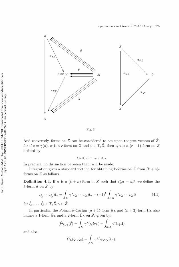
as πYZ(γ) = πYZ γ. We denote by πXY the unique mapping from Y to X suchthat πXZ = πXY πYZ (see Fig. 3).

A tangent vector v at γ ∈ Z can be seen as a vector field along γ, that is,v: M → TZ such that τZ v = γ, where τZ : TZ → Z is the canonical projection.Therefore, we identify vectors in TγZ with vector fields on γ(M). Thus, a vectorfield ξZ on Z induces a vector field ξZ on Z, where for every γ ∈ Z, its representativetangent vector at γ ∈ Z is given by

ξZ(γ) = ξZ γ.

Int.

J. G

eom

. Met

hods

Mod

. Phy

s. 2

004.

01:6

51-7

10. D

ownl

oade

d fr

om w

ww

.wor

ldsc

ient

ific

.com

by B

AY

LO

R U

NIV

ER

SIT

Y o

n 06

/24/

14. F

or p

erso

nal u

se o

nly.



Z

Y

X

πXZ

πYZ

πXY

M

Z

Y

X

Z

Y

X

πXZ

πY Z

πXY

Fig. 3.

And conversely, forms on Z can be considered to act upon tangent vectors of Z,for if z = γ(u), α is a r-form on Z and v ∈ TγZ, then ιvα is a (r − 1)-form on Z

defined by

(ιvα)z := ιv(u)αz.

In practice, no distinction between them will be made.Integration gives a standard method for obtaining k-forms on Z from (k + n)-

forms on Z as follows.

Definition 4.4. If α is a (k + n)-form in Z such that i∗Bα = dβ, we define thek-form α on Z by

ιζ1· · · ιζk

αγ =∫

M

γ∗ιζ1 · · · ιζkαα − (−1)k

∫∂M

γ∗ιζ1 · · · ιζkβ (4.1)

for ζ1, . . . , ζk ∈ TγZ, γ ∈ Z.

In particular, the Poincare–Cartan (n + 1)-form ΘL and (n + 2)-form ΩL alsoinduce a 1-form ΘL and a 2-form ΩL on Z, given by:

(ΘL)γ(ξ) =∫

M

γ∗(ιξΘL) +∫

∂M

γ∗(ιξΠ)

and also

ΩL(ξ1, ξ2) =∫

M

γ∗(ιξ2ιξ1ΩL).

Int.

J. G

eom

. Met

hods

Mod

. Phy

s. 2

004.

01:6

51-7

10. D

ownl

oade

d fr

om w

ww

.wor

ldsc

ient

ific

.com

by B

AY

LO

R U

NIV

ER

SIT

Y o

n 06

/24/

14. F

or p

erso

nal u

se o

nly.



Lemma 4.5. If ξ is a vector field on Z defined from a vector field ξ on Z, and α

is an n-form on Z such that i∗Bα = dβ then

dα(ξ)γ = (£ξα)γ =∫

M

γ∗(£ξα) −∫

∂M

γ∗(£ξβ).

Proof. First observe that α is a function. In this case, if cZ(t) is a curve such thatcZ(0) = γ and cZ(0) = ξ(γ), then

dα(ξ)γ = ξγ(α) =d

dt(α cZ(t))

∣∣∣∣t=0

=d

dt

[∫M

(cZ(t)∗α) −∫

∂M

(cZ(t)∗β)]∣∣∣∣

t=0

=∫

M

d

dt(cZ(t)∗α)

∣∣∣∣t=0

−∫

∂M

d

dt(cZ(t)∗β)

∣∣∣∣t=0

=∫

M

γ∗(£ξα) −∫

∂M

γ∗(£ξβ).

The previous result can be also extended for forms of higher degree, and forarbitrary fibrations over X .

Let ξ be a complete vector field on a fibration W over X , and let us denote byW certain space of embeddings in W , and by ξ the vector field defined on W fromξ (that is, ξ(γ)(u) = ξ(γ(u))).

Fix γ ∈ W . For every u ∈ M , consider an integral curve cu of ξ through γ(u),that is,

cu(0) = γ(u)

cu(0) = ξ(γ(u)).

Let us define a curve c on W by

c(t)(u) = cu(t).

Then we have that

Proposition 4.6. c is an integral curve of ξ through γ.

Proof. To see this, we just have to compute

c(0)(u) = cu(0) = γ(u)

and

˙c(0)(u) =d

dt(c(t))∣∣∣∣t=0

(u) =d

dt(c(t)(u))

∣∣∣∣t=0

=d

dtcu(t)∣∣∣∣t=0

= cu(t) = ξ(γ(u)) = ξ(γ)(u).

c will be said to be the associated curve to the flow given by the cu’s.In particular, if we also have a diffeomorphism F : W → W , it is easy to see

that the curve (denoted by F c) associated to the family F cu is precisely F c.To see this, and using the preceding notation, note first that

F c(t)(u) = (F c)u(t) = (F cu)(t) = F (cu(t)) = F (c(t)(u)) = (F c(t))(u),

Int.

J. G

eom

. Met

hods

Mod

. Phy

s. 2

004.

01:6

51-7

10. D

ownl

oade

d fr

om w

ww

.wor

ldsc

ient

ific

.com

by B

AY

LO

R U

NIV

ER

SIT

Y o

n 06

/24/

14. F

or p

erso

nal u

se o

nly.



from which we deduce:

Corollary 4.7. If F : W → W is a diffeomorphism, then TF (ξ) = TF (ξ).

The next step is to study the pullback of forms.

Proposition 4.8. If F : W → W is a diffeomorphism, and α is a (n + k)-form onW, such that i∗Bα = dβ, then

F ∗α = F ∗α.

Proof. Let V1, . . . , Vk ∈ TF−1(γ)W . We have that

ιV1. . . ιVk

F ∗α = α(T F (V1), . . . , T F (Vk)) = α(T F (V1), . . . , ˜TF (Vk)

)=∫

M

γ∗ιTF (V1) . . . ιTF (Vk)α − (−1)k

∫∂M

γ∗ιTF (V1) . . . ιTF (Vk)β

=∫

M

(F−1 γ)∗F ∗ιTF (V1) . . . ιTF (Vk)α

− (−1)k

∫∂M

(F−1 γ)∗F ∗ιTF (V1) . . . ιTF (Vk)β

=∫

M

(F−1 γ)∗ιV1 · · · ιVkF ∗α − (−1)k

∫∂M

(F−1 γ)∗ιV1 · · · ιVkF ∗β

= ιV1· · · ιVk

F ∗α.

Finally:

Proposition 4.9. If ξ is a vector field on W , then

£ξα = £ξα.

Proof. Let V1, . . . , Vk ∈ TγW , and denote by φt the flow of ξ. Then we have that

ιV1· · · ιVk

£ξα = ιV1· · · ιVk

d

dtφ∗

t α

∣∣∣∣t=0

= ιV1· · · ιVk

d

dtφ∗

t α

∣∣∣∣t=0

=d

dt

(ιV1

· · · ιVkφ∗

t α)∣∣∣∣

t=0

=d

dt

(∫M

ιV1 · · · ιVkφ∗

t α − (−1)k

∫∂M

ιV1 · · · ιVkφ∗

t β

)∣∣∣∣t=0

=∫

M

ιV1 · · · ιVk

d

dt(φ∗

t α)∣∣∣∣t=0

− (−1)k

∫∂M

ιV1 · · · ιVk

d

dt(φ∗

t β)∣∣∣∣t=0

=∫

M

ιV1 · · · ιVk£ξα − (−1)k

∫∂M

ιV1 · · · ιVk£ξβ

= ιV1· · · ιVk

£ξα

where for the last bit just notice that i∗B£ξα = £ξi∗Bα = £ξdβ = d£ξβ.

Int.

J. G

eom

. Met

hods

Mod

. Phy

s. 2

004.

01:6

51-7

10. D

ownl

oade

d fr

om w

ww

.wor

ldsc

ient

ific

.com

by B

AY

LO

R U

NIV

ER

SIT

Y o

n 06

/24/

14. F

or p

erso

nal u

se o

nly.



Back to the fibration Z → X , the consistency of our definition of forms respectto the exterior derivative is ensured by the following proposition.

Proposition 4.10. If α is an n-form or an (n + 1)-form, then

dα = dα.

In particular,

ΩL := −dΘL.

Proof. For n-forms we use the previous lemma

(dα)γ(ξ) =∫

M

γ∗£ξα −∫

∂M

γ∗£ξβ

=∫

M

γ∗ιξdα +∫

M

γ∗dιξα −∫

∂M

γ∗(iξdβ + diξβ)

=∫

M

γ∗ιξdα = (dα)γ(ξ).

For (n + 1)-forms:

dα(ξ, ζ)γ = ξ(α(ζ)) − ζ(α(ξ)) − α([ζ, ξ])γ

=∫

M

γ∗£ξ(ιζα) − £ζ(ιξα) − ι[ξ,ζ]α

+∫

∂M

γ∗£ξ(ιζβ) − £ζ(ιξβ) − ι[ξ,ζ]β

=∫

M

γ∗ιζιξdα − dιζιξα

+∫

∂M

γ∗ιζιξdβ − dιζιξβ

=∫

M

γ∗(ιζιξdα) −∫

∂M

γ∗(ιζιξ(dβ − α))

=∫

M

γ∗(ιζιξdα)

= dα(ξ, ζ)γ .

4.2. The de Donder equations in the space of Cauchy data

The de Donder equations of Field Theories have a presymplectic counterpart inthe spaces of Cauchy data. The relationship between both can be found in [3] (seealso [28]), and requires the definition of a slicing of the base manifold X .

Definition 4.11. We say that a curve cX in X defined on a domain I ⊆ R splits X

if the mapping Φ: I×M → X, such that Φ(t, u) = cX(t)(u), is a diffeomorphism. Inparticular, the partial mapping Φ(t) (defined by Φ(t, ·)(u) = Φ(t, u)) is an elementof X for all t ∈ I. In this case, cX is said to be a slicing.

Int.

J. G

eom

. Met

hods

Mod

. Phy

s. 2

004.

01:6

51-7

10. D

ownl

oade

d fr

om w

ww

.wor

ldsc

ient

ific

.com

by B

AY

LO

R U

NIV

ER

SIT

Y o

n 06

/24/

14. F

or p

erso

nal u

se o

nly.



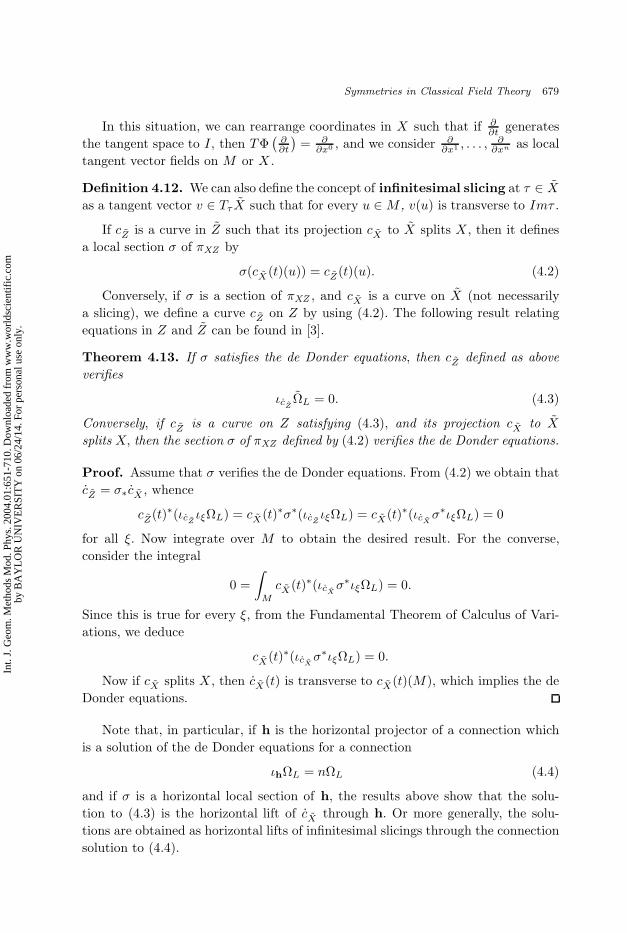
In this situation, we can rearrange coordinates in X such that if ∂∂t generates

the tangent space to I, then TΦ(

∂∂t

)= ∂

∂x0 , and we consider ∂∂x1 , . . . , ∂

∂xn as localtangent vector fields on M or X.

Definition 4.12. We can also define the concept of infinitesimal slicing at τ ∈ X

as a tangent vector v ∈ Tτ X such that for every u ∈ M , v(u) is transverse to Imτ .

If cZ is a curve in Z such that its projection cX to X splits X , then it definesa local section σ of πXZ by

σ(cX(t)(u)) = cZ(t)(u). (4.2)

Conversely, if σ is a section of πXZ , and cX is a curve on X (not necessarilya slicing), we define a curve cZ on Z by using (4.2). The following result relatingequations in Z and Z can be found in [3].

Theorem 4.13. If σ satisfies the de Donder equations, then cZ defined as aboveverifies

ιcZΩL = 0. (4.3)

Conversely, if cZ is a curve on Z satisfying (4.3), and its projection cX to X

splits X, then the section σ of πXZ defined by (4.2) verifies the de Donder equations.

Proof. Assume that σ verifies the de Donder equations. From (4.2) we obtain thatcZ = σ∗cX , whence

cZ(t)∗(ιcZιξΩL) = cX(t)∗σ∗(ιcZ

ιξΩL) = cX(t)∗(ιcXσ∗ιξΩL) = 0

for all ξ. Now integrate over M to obtain the desired result. For the converse,consider the integral

0 =∫

M

cX(t)∗(ιcXσ∗ιξΩL) = 0.

Since this is true for every ξ, from the Fundamental Theorem of Calculus of Vari-ations, we deduce

cX(t)∗(ιcXσ∗ιξΩL) = 0.

Now if cX splits X , then cX(t) is transverse to cX(t)(M), which implies the deDonder equations.

Note that, in particular, if h is the horizontal projector of a connection whichis a solution of the de Donder equations for a connection

ιhΩL = nΩL (4.4)

and if σ is a horizontal local section of h, the results above show that the solu-tion to (4.3) is the horizontal lift of cX through h. Or more generally, the solu-tions are obtained as horizontal lifts of infinitesimal slicings through the connectionsolution to (4.4).

Int.

J. G

eom

. Met

hods

Mod

. Phy

s. 2

004.

01:6

51-7

10. D

ownl

oade

d fr

om w

ww

.wor

ldsc

ient

ific

.com

by B

AY

LO

R U

NIV

ER

SIT

Y o

n 06

/24/

14. F

or p

erso

nal u

se o

nly.



4.3. The singular case

For a singular Lagrangian, we cannot guarantee the existence of a curve cZ in Z asa solution of the de Donder equations in Z.

Therefore, we propose an algorithm similar to that of a general presymplecticspace (developed in [26, 30, 31]; see also [8, 45, 47] for the time dependent case),where to the condition that defines the manifold obtained in each step (which isthe existence of a tangent vector verifying the de Donder equations), we add thefact that this tangent vector must project onto an infinitesimal slicing.

Naming Z1 := Z, we define Z2 and the subsequent subsets (requiring them tobe submanifolds) as follows:

Z2 := γ ∈ Z1 | ∃v ∈ TγZ1 such that TπXZ(v)

is an infinitesimal slicing and ιvΩL|γ = 0Z3 := γ ∈ Z2 | ∃v ∈ TγZ2 such that TπXZ(v)

is an infinitesimal slicing and ιvΩL|γ = 0. . .

In the favorable case, the algorithm will stop at a certain final non-zero dimen-sional constraint submanifold Zf .

This algorithm is closely related to the algorithm in the finite dimensionalspaces. We turn now to state the link between them.

Proposition 4.14. Suppose that we have v ∈ TγZ1 such that TπXZ(v) is aninfinitesimal slicing and ιvΩL|γ = 0. Then, for every u ∈ M we have that

Hγ(u) := Tuγ(TuM) ⊕ 〈v(u)〉is a horizontal subspace of Tγ(u)Z whose horizontal projector h verifies the de Don-der equations for connections satisfying (4.4) at γ(u):

ιhΩL|γ(u) = nΩL|γ(u).

Proof. The fact that v projects onto an infinitesimal slicing guarantees that Hγ(u)

is indeed horizontal.The other hypothesis states that

γ∗(ιξιvγ(u)ΩL) = 0

for every ξ ∈ Tγ(u)Z, that is, if 〈v1, v2, . . . , vn〉 is a basis for TuM , then

ιξιvγ(u)ΩL(Tuγ(v1), Tuγ(v2), . . . , Tuγ(vn)) = 0,

or in other words,

ΩL(ξ, H1, H2, . . . , Hn+1) = 0

Int.

J. G

eom

. Met

hods

Mod

. Phy

s. 2

004.

01:6

51-7

10. D

ownl

oade

d fr

om w

ww

.wor

ldsc

ient

ific

.com

by B

AY

LO

R U

NIV

ER

SIT

Y o

n 06

/24/

14. F

or p

erso

nal u

se o

nly.



for every ξ ∈ Tγ(u)Z and every collection H1, H2, . . . , Hn+1 of horizontal tangentvectors.

We want to prove that ιhΩL|γ(u) = nΩL|γ(u), or equivalently, ιξιhΩL|γ(u) =nιξΩL|γ(u), for every ξ ∈ Tγ(u)Z.

From the previous remarks, we see that the condition results to be true when itis evaluated on n + 1 horizontal vector fields.

Suppose that V1 is a vertical tangent vector to γ(u). Then (as h(V1) = 0),

ιhΩL(ξ, V1, H1, . . . , Hn) = ΩL(h(ξ), V1, H1, . . . , Hn) + nΩL(ξ, V1, H1, . . . , Hn)

where the first term vanishes due to the previous remarks. Thus, the expressionholds when applied to any two tangent vectors, and to any n horizontal tangentvectors.

For the next step, having two vertical vectors, remember that ΩL is annihilatedby three vertical tangent vectors. Therefore,

ιhΩL(ξ, V1, V2, H1, . . . , Hn−1)

= ΩL(h(ξ), V1, V2, H1, . . . , Hn−1) + (n − 1)ΩL(ξ, V1, V2, H1, . . . , Hn−1)

= ΩL(ξ, V1, V2, H1, . . . , Hn−1) + (n − 1)ΩL(ξ, V1, V2, H1, . . . , Hn−1)

= nΩL(ξ, V1, V2, H1, . . . , Hn−1)

Finally, from the mentioned properties of ΩL, the expression also holds for a highernumber of vertical tangent vectors, and so the expression holds in general.

As an immediate result, we have that:

Corollary 4.15. If γ ∈ Z2, then Imγ ⊆ Z2.

And in general:

Proposition 4.16. If γ ∈ Zi, then Imγ ⊆ Zi.

Proof. If γ ∈ Zi (which implies that there exists v ∈ T Zi such that ιvΩL|γ = 0),then for every u ∈ M we define Hγ(u) := Tγu(TuM) ⊕ 〈v(u)〉.

We need to justify in each step that Hγ(u) ⊆ Tγ(u)Zi, which amounts to provethat Tγu(TuM) ⊆ Tγ(u)Zi and v(u) ∈ Tγ(u)Zi. The first assertion is true by con-struction of the subsets.

To see that v(u) ∈ Tγ(u)Zi, we proceed inductively, starting with i = 2, forwhich the result is true because of the preceding corollary.

We assume it to be true for all the steps until the i-th, and we prove thatv(u) ∈ Tγ(u)Zi+1.

As γ ∈ Zi+1, there exists v ∈ TγZi such that ιvΩL = 0. Thus, there exists acurve c: (−ε, ε) → Zi (and thus Im(c)(t) ⊆ Zi) such that c(0) = γ and c(0) = v.We deduce that v(u) ∈ Tγ(u)Zi.

Int.

J. G

eom

. Met

hods

Mod

. Phy

s. 2

004.

01:6

51-7

10. D

ownl

oade

d fr

om w

ww

.wor

ldsc

ient

ific

.com

by B

AY

LO

R U

NIV

ER

SIT

Y o

n 06

/24/

14. F

or p

erso

nal u

se o

nly.



Remark 4.17. Suppose now that X admits a slicing. In the case in which z ∈ Zi

is such that πXZ (z) belongs to the image of the slicing, and hz is integrable, thenthere exists γ ∈ Zi, and u ∈ M such that γ(u) = z.

As before, we first prove the case i = 2. If σ is a horizontal local section ofh at z, then we use the slicing to define the curve cZ(t), which verifies the de Donderequations in Z, and projects onto the slicing. Therefore we can take γ = cZ(t) forsome t.

For the case i > 2, simply observe that if Hγ(u) ⊆ Tγ(u)Zi, then cZ(t)(u′) mustbe tangent to Zi for all u′ ∈ M , and a very similar argument to that of the precedingsection proves that γ = cZ(t) ∈ Zi.

4.4. Brackets

Notice that, in general, the only fact over ΩL that we can guarantee is thatit is presymplectic, as we cannot guarantee the existence nor the uniqueness ofHamiltonian vector fields associated with functions defined on Z. For further detailssee [50] and [51].

Definition 4.18. Given a function f in Z and a vector field ξ on Z, we shall saythat f is a Hamiltonian function, and that ξ is a Hamiltonian vector fieldfor f if

ιξΩL = df.

Proposition 4.19. If α is a Hamiltonian n-form in Z for ΩL which is exact on∂Z, say α|∂Z = dβ, then α is a Hamiltonian function on Z for ΩL. More precisely,if Xα is a Hamiltonian vector field for α, then Xα defined on Z by

[Xα(γ)](u) = Xα(γ(u))

is a Hamiltonian vector field for α.

Proof. Take a tangent vector ξ to Z, then by Lemma 4.5

(dα)(ξ)|γ =∫

M

γ∗(£ξα) −∫

∂M

γ∗(£ξβ)

=∫

M

γ∗ιξ dα +∫

M

γ∗dιξα −∫

∂M

γ∗ιξ dβ

=∫

M

γ∗ιξ dα =∫

M

γ∗ιξιXαΩL = ιXαΩL(ξ)|γ ,

which proves that dα = ιXα ΩL.

If f is a Hamiltonian function on Z, then its associated Hamiltonian vector fieldis defined up to an element in the kernel of ΩL, therefore we can define the bracketoperation for these functions as follows.

Int.

J. G

eom

. Met

hods

Mod

. Phy

s. 2

004.

01:6

51-7

10. D

ownl

oade

d fr

om w

ww

.wor

ldsc

ient

ific

.com

by B

AY

LO

R U

NIV

ER

SIT

Y o

n 06

/24/

14. F

or p

erso

nal u

se o

nly.



Definition 4.20. If f and g are Hamiltonian functions on Z, with associatedHamiltonian vector fields Xf and Xg, then we define:

f, g := ΩL(Xf , Xg).

Proposition 4.21. Assume that ∂X = ∅, then if α1 and α2 are Hamiltoniann-forms, then

α1, α2 = α1, α2.

Proof.

α1, α2 = ΩL(Xα1 , Xα2) =∫

M

γ∗ιXα2ιXα1

ΩL =∫

M

γ∗α1, α2 = α1, α2.

In [6, 19] and [25] the authors explore the properties of a generalization of thisbracket, which satisfies the graded versions of several properties, such as skew-symmetry and Jacobi identity.

Remark 4.22. We could alternatively use the space of Cauchy data Z∗, defined inthe obvious way. But nothing different or new would be obtained. In fact, assumefor simplicity that L is hyperregular. Then we would have a diffeomorphism legL:Z → Z∗ defined by the following composition:

legL(γ) = legL γ

for all γ ∈ Z.If the Lagrangian is not regular, but at least is almost regular, we invite to the

reader to develop the corresponding scheme. The only delicate point is that we haveto consider the second order problem in the Lagrangian side, so that legL: Z → Z∗

becomes a fibration.In what follows, we shall emphasize the discussion in the Lagrangian side, since,

as we have shown, the equivalence with the Hamiltonian side is obvious.

5. Symmetries and Noether’s Theorems

We are now interested in studying the presence of symmetries which would even-tually produce preserved quantities, and allow us to reduce the complexity of thedynamical system and to obtain valuable information about its behavior. For everytype of symmetry, there will be a form of Noether’s theorem, which will show upthe preserved quantity obtained from it (see [60]).

We shall suppose that we are in the regular Lagrangian case, unless statedotherwise.

In our framework for field theory, we define a preserved quantity in the followingmanner:

Definition 5.1. A preserved quantity for the Euler–Lagrange equationsis an n-form α on Z such that (j1φ)∗dα = 0 for every solution φ of the

Int.

J. G

eom

. Met

hods

Mod

. Phy

s. 2

004.

01:6

51-7

10. D

ownl

oade

d fr

om w

ww

.wor

ldsc

ient

ific

.com

by B

AY

LO

R U

NIV

ER

SIT

Y o

n 06

/24/

14. F

or p

erso

nal u

se o

nly.



Euler–Lagrange equations. If α is a preserved quantity, then α is called its associ-ated momentum.

Notice that if α is a preserved quantity, and Λ is a closed form, then α+Λ is alsoa preserved quantity. Similarly, if γ is an n-form which belongs to the differentialideal I(C), then α + γ is also a preserved quantity (see [60] for further discussion).

We turn now to obtain preserved quantities from symmetries.

5.1. Symmetries of the Lagrangian

We shall define the notion of symmetry based on the the variation of the Poincare–Cartan (n+1)-form along prolongations of vector fields. Suppose that ξY is a vectorfield defined on Y , and abbreviate by F the function such that

£ξ(1)Y

L − Fη ∈ I(C)

having local expression

F = ξ(1)Y (L) +

(∂ξµ

Y

∂xµ+ zi

ν

∂ξνY

∂yi

)L. (5.1)

After a lengthy computation we get

£ξ(1)Y

ΘL = Fη +∂F

∂ziµ

θi ∧ dnxµ + zjν

(∂ξν

Y

∂yj

∂L

∂ziµ

− ∂ξµY

∂yj

∂L

∂ziν

)θi ∧ dnxµ

− ∂ξνY

∂yj

∂L

∂ziµ

θi ∧ dyj ∧ dn−1xνµ. (5.2)

Definition 5.2. A vector field ξY on Y is said to be an infinitesimal symmetryof the Lagrangian or a variational symmetry if £

ξ(1)Y

ΘL ∈ I(C) (the differen-

tial ideal generated by the contact forms), and ξ(1)Y is also tangent to B and verifies

£ξ(1)Y |BΠ = 0.

We shall only deal with infinitesimal symmetries of the Lagrangian, so for brevitythey will be referred simply as symmetries of the Lagrangian.

From the definition and the expression (5.2), it is obvious to see that:

Proposition 5.3. If a vector field ξY on Y is a symmetry of the Lagrangian, thenF = 0 (where F was defined in (5.1)).

Remark 5.4. In our construction, we choose as definition of the Poincare–Cartan(n + 1)-form:

ΘL = L + (Sη)∗(dL)

or, in fibered coordinates

ΘL = L dn+1x +∂L

∂ziµ

θi ∧ dnxµ.

Int.

J. G

eom

. Met

hods

Mod

. Phy

s. 2

004.

01:6

51-7

10. D

ownl

oade

d fr

om w

ww

.wor

ldsc

ient

ific

.com

by B

AY

LO

R U

NIV

ER

SIT

Y o

n 06

/24/

14. F

or p

erso

nal u

se o

nly.



If n > 0 it is possible to generalize the construction of the Poincare–Cartan (n+1)-form in several different ways. The unique requirement is that the resulting πYZ -semibasic (n + 1)-form be Lepage-equivalent to L, that is,

Θ − L ∈ I(C)

and iV dΘ ∈ I(C) where V is an arbitrary πYZ -vertical vector field. Locally,

Θ = ΘL + · · · (5.3)

where the dots signify terms which are at least two-contact (see [2, 10, 39, 43]).Obviously, all them gives us the same Euler–Lagrange equations.

Therefore, we may substitute in Definitions 5.2, 5.8 and 5.13 the Poincare–Cartan (n+1)-form by any (n+1)-form which is Lepage-equivalent to ΘL. Obviously,the symmetries of the Euler–Lagrange equations are independent of the class ofLepagian (n + 1)-form appearing in their definition.

We also have the following two special cases, which are easily computed fromthe expression of F .

Proposition 5.5. If ξY is a projectable symmetry of the Lagrangian(TπXY (ξY )

is a well defined vector field, or locally ∂ξµY

∂yi = 0), or if dimX = 1 (n = 0), then

£ξ(1)Y

ΘL = 0

or, equivalently,

£ξ(1)Y

L = 0.

Therefore,

ξ(1)Y (L) = −

∑µ

dξµY

dxµL.

And as a direct consequence of Proposition 2.5, we have:

Proposition 5.6. The symmetries of the Lagrangian form a Lie subalgebraof X(Y ).

Theorem 5.7 (Noether’s Theorem). If ξY is a symmetry of the Lagrangian,

then ιξ(1)Y

ΘL is a preserved quantity, which is exact on the boundary.

Proof. We have that

£ξ(1)Y

ΘL = −ιξ(1)Y

ΩL + dιξ(1)Y

ΘL.

If φ is a solution of the Euler–Lagrange equations, then

0 = (j1φ)∗£ξ(1)Y

ΘL = −(j1φ)∗ιξ(1)Y

ΩL + (j1φ)∗dιξ(1)Y

ΘL,

Int.

J. G

eom

. Met

hods

Mod

. Phy

s. 2

004.

01:6

51-7

10. D

ownl

oade

d fr

om w

ww

.wor

ldsc

ient

ific

.com

by B

AY

LO

R U

NIV

ER

SIT

Y o

n 06

/24/

14. F

or p

erso

nal u

se o

nly.



where the first term vanishes by the intrinsic Euler–Lagrange equations (seeProposition 2.16).

Finally, to see that it is exact on the boundary, notice that from the boundaryproperty of a symmetry of the Lagrangian we infer that ι

ξ(1)Y |B

dΠ = −dιξ(1)Y |B

Π,

and from this we get

i∗B(ιξ(1)Y

ΘL) = ιξ(1)Y |B

dΠ = −dιξ(1)Y |B

Π.

Observe that without the boundary condition, we obtain that (j1φ)∗dιξ(1)Y

ΘL=0,but we cannot be sure that it is exact on the boundary.

The preserved quantity can be written in local coordinates as([L − zi

µ

∂L

∂ziµ

]ξνX +

∂L

∂ziν

ξiY

)dnxν − ∂L

∂ziµ

ξνXdyi ∧ dn−1xµν .

5.2. Noether symmetries

Definition 5.8. A vector field ξY on Y is said to be a Noether symmetry ora divergence symmetry if there exists an n-form on Y whose pullback α to Z

(that must be exact α = dβ on B) verifies £ξ(1)Y

ΘL−dα ∈ I(C), and ξ(1)Y is tangent

to B and verifies £ξ(1)Y |BΠ = 0.

The relation dyi = θi + ziµdxµ allows us to write α locally as follows

α = αµdx0 ∧ · · · ∧ dxµ ∧ · · · ∧ dxn + θ

for θ ∈ I(C) and

dα −∑

µ

(∂αµ

∂xµ+ zi

µ

∂αµ

∂yi

)η ∈ I(C).

Therefore, if we define:

F = F +∑

µ

(∂αµ

∂xµ+ zi

µ

∂αµ

∂yi

)then:

Proposition 5.9. If a vector field ξY on Y is a Noether symmetry, then F = 0.

Similarly,

Proposition 5.10. (i) If ξY is a πXY −projectable Noether symmetry, then

£ξ(1)Y

ΘL = dα.

Int.

J. G

eom

. Met

hods

Mod

. Phy

s. 2

004.

01:6

51-7

10. D

ownl

oade

d fr

om w

ww

.wor

ldsc

ient

ific

.com

by B

AY

LO

R U

NIV

ER

SIT

Y o

n 06

/24/

14. F

or p

erso

nal u

se o

nly.



Furthermore,

ξ(1)Y (L) = −

∑µ

(dξµ

Y

dxµL +

dαµ

dxµ

).

(ii) If dim X = 1 and ξY is a Noether symmetry then

£ξ(1)Y

ΘL = dα.

Proposition 5.11. Noether symmetries form a Lie subalgebra of X(Y ), containingthe Lie algebra of the symmetries of the Lagrangian.

Proof.

£[ξ

(1)Y ,ζ

(1)Y ]

ΘL = £ξ(1)Y

£ζ(1)Y

ΘL − £ζ(1)Y

£ξ(1)Y

ΘL = £ξ(1)Y

(dα2 + θ2) − £ζ(1)Y

(dα1 + θ1)

= d(£ξ(1)Y

α2 − £ζ(1)Y

α1) + £ξ(1)Y

θ2 − £ζ(1)Y

θ1

and £ξ(1)Y

θ2 − £ζ(1)Y

θ1 ∈ I(C).

Finally, since ξ(1)Y and ζ

(1)Y are tangent to B, then [ξ(1)

Y , ζ(1)Y ] is also tangent to B.

We also have that £[ξ

(1)Y ,ζ

(1)Y ]|B

Π = £ξ(1)Y |B

£ζ(1)Y |B

Π−£ζ(1)Y |B

£ξ(1)Y |B

Π = 0 on B, and

that if α1 and α2 are exact on B, so is £ξ(1)Y |B

α2 − £ζ(1)Y |B

α1.

The following Noether’s theorem:

Theorem 5.12 (Noether’s Theorem). If ξY is a Noether symmetry, thenιξ(1)Y

ΘL − α is a preserved quantity which is exact on the boundary.

is proved analogously as we did for the symmetries of the Lagrangian. We justremark a slight modification introduced to see that it is exact on the boundary:

i∗B(ιξ(1)Y

ΘL − α)

= ιξ(1)Y |B

dΠ − dβ = d(− ι

ξ(1)Y |B

Π − β).

5.3. Cartan symmetries

Definition 5.13. A vector field ξZ on Z is said to be a Cartan symmetry if itsflow preserves the differential ideal I(C) (in other words, ψ∗

Z,tθi ∈ I(C), or locally,

£ξZI(C) ⊆ I(C)), and there exists an n-form α on Z (that must be exact α = dβ

on B) such that £ξZ ΘL − dα ∈ I(C), ξZ is tangent to B and verifies £ξZ |BΠ = 0.

If ξY is a Noether symmetry, then its 1-jet prolongation is a Cartan symmetry.Conversely, it is obvious that a projectable Cartan symmetry is the 1-jet prolonga-tion of its projection, which is therefore a Noether symmetry.

Proposition 5.14. The Cartan symmetries form a subalgebra of X(Z).

We also have

Theorem 5.15 (Noether’s Theorem). If ξZ is a Cartan symmetry, thenιξZ ΘL − α is a preserved quantity which is exact on the boundary.

Int.

J. G

eom

. Met

hods

Mod

. Phy

s. 2

004.

01:6

51-7

10. D

ownl

oade

d fr

om w

ww

.wor

ldsc

ient

ific

.com

by B

AY

LO

R U

NIV

ER

SIT

Y o

n 06

/24/

14. F

or p

erso

nal u

se o

nly.



We also have the obvious relations between the different types of symmetriesthat we have exposed here. Every symmetry of the Lagrangian is a Noether sym-metry. And the 1-jet prolongation of any Noether symmetry is a Cartan symmetry.

And finally,

Proposition 5.16. The flow of Cartan symmetries maps solutions of the Euler–Lagrange equations into solutions of the Euler–Lagrange equations.

Proof. Let ψtZ be the flow of a Cartan symmetry ξZ .

For any section φ ∈ Γ(π), we can locally define

ψtφ,X := πXZ ψt

Z j1φ.

ψ0φ,X = IdX , whence for small t′s, ψt

φ,X is a diffeomorphism. Analogously, we define

ψtφ,Y := πYZ ψt

Z j1φ πXY .

With the same argument we see that for small t′s, ψtφ,Y is a diffeomorphism as well.

If φ is a solution of the Euler–Lagrange equation, then the flow transforms φ

into

ψtφ,Y φ (ψt

φ,X)−1.

Now, for θ ∈ C,

(ψtZ j1φ (ψt

φ,X)−1)∗θ = ((ψtφ,X)−1)∗(j1φ)∗(ψt

Z)∗θ = 0

as ξZ is a Cartan symmetry. This means that ψtZ j1φ (ψt

φ,X)−1 is the 1-jetprolongation of its projection to Y ,

πYZ ψtZ j1φ (ψt

φ,X)−1 = ψtφ,Y φ (ψt

φ,X)−1.

In other words,

j1(ψtφ,Y φ (ψt

φ,X)−1) = ψtZ j1φ (ψt

φ,X)−1.

Now we need to see that the transformed solution verifies the Euler–Lagrange equa-tions. The preceding equation shows that, being the symmetry tangent to B, theboundary condition will be satisfied.

In addition, for every compact (n+1)-dimensional submanifold C, and every ver-tical vector field ξ ∈ V(π), which is annihilated at ∂C (and therefore, so does ξ(1)),∫

(ψtφ,X)(C)

(j1(ψtφ,Y φ (ψt

φ,X)−1))∗£ξ(1)ΘL

=∫

(ψtφ,X )(C)

(ψtZ j1φ (ψt

φ,X)−1)∗£ξ(1)ΘL

=∫

C

(ψtZ j1φ)∗£ξ(1)ΘL =

∫C

(j1φ)∗(ψtZ)∗£ξ(1)ΘL

Int.

J. G

eom

. Met

hods

Mod

. Phy

s. 2

004.

01:6

51-7

10. D

ownl

oade

d fr

om w

ww

.wor

ldsc

ient

ific

.com

by B

AY

LO

R U

NIV

ER

SIT

Y o

n 06

/24/

14. F

or p

erso

nal u

se o

nly.



by means of a change of variable. The annihilation of the preceding expression isinfinitesimally equivalent to the annihilation of∫

C

(j1φ)∗£ξZ £ξ(1)ΘL =∫

C

(j1φ)∗£[ξZ,ξ(1)]ΘL −∫

C

(j1φ)∗£ξ(1)£ξZ ΘL

and we conclude by seeing that∫C

(j1φ)∗£[ξZ ,ξ(1)]ΘL = −∫

C

(j1φ)∗ι[ξZ ,ξ(1)]ΩL +∫

C

(j1φ)∗dι[ξZ ,ξ(1)]ΘL = 0

where the first term vanishes because φ is a solution of Euler–Lagrange equations,and the second term vanishes due to the boundary condition on ξ; and∫

C

(j1φ)∗£ξ(1)£ξZ ΘL =∫

C

(j1φ)∗£ξ(1)(dα + θ)

=∫

∂C

(j1φ)∗£ξ(1)α +∫

C

(j1φ)∗£ξ(1)θ = 0

where the first term vanishes again by the boundary condition on ξ.

5.4. Symmetries for the de Donder equations

In the discussion of the preceding section, we have used on Noether’s theorem thefact that, for a solution φ of the Euler–Lagrange equations, we have

(j1φ)∗θ = 0

for elements θ of the differential ideal generated by the contact forms. However,this result is no longer true for general solutions of the de Donder equations (morespecifically, when the Lagrangian is not regular). In other words, if σ is a solutionof the de Donder equations, then we do not necessarily have

σ∗θ = 0

for θ ∈ I(C).Therefore, our definition of symmetry must be more restrictive when we are

dealing with solutions of the de Donder equations.

Definition 5.17. A preserved quantity for the de Donder equations is ann-form α on Z such that σ∗dα = 0 for every solution σ of the de Donder equations.If α is a preserved quantity, then α is called its associated momentum.

Also note that if α is a preserved quantity and β is a closed n-form, then α + β

is also a preserved quantity.From Eq. (2.7) we can easily deduce the following.

Proposition 5.18. Let h be a solution of the connection equation (2.6). Then α

is a preserved quantity for the de Donder equations if and only if dα is annihilatedby any n horizontal tangent vectors at each point.

Int.

J. G

eom

. Met

hods

Mod

. Phy

s. 2

004.

01:6

51-7

10. D

ownl

oade

d fr

om w

ww

.wor

ldsc

ient

ific

.com

by B

AY

LO

R U

NIV

ER

SIT

Y o

n 06

/24/

14. F

or p

erso

nal u

se o

nly.



Definition 5.19. We have the following definitions of symmetries for the deDonder equations:

(i) A vector field ξY on Y is said to be a symmetry of the Lagrangian, or avariational symmetry if

£ξ(1)Y

ΘL = 0

and ξ(1)Y is tangent to B and verifies £

ξ(1)Y |BΠ = 0.

(ii) A vector field ξY on Y is said to be a Noether symmetry, or a divergencesymmetry if

£ξ(1)Y |BΘL = dα

where α is the pullback to Z of an n-form on Y (that must be exact α = dβ

on B), ξ(1)Y is tangent to B and verifies £

ξ(1)Y |B

Π = 0.

(iii) A vector field ξZ on Z is a Cartan symmetry if

£ξZ ΘL = dα

where α is a n-form on Z (that is exact α = dβ on B) (or, equivalently, ifthere is an n-form α′ such that

ιξZ ΩL = dα′,

we can put α′ = α + ιξZ ΘL, in other words, if ξZ is a Hamiltonian vectorfield), ξZ is tangent to B and verifies £ξZ |BΠ = 0.

There is an obvious relation between these types of symmetries, completelyanalogous to those between the symmetries for the Euler–Lagrange equations, thatis, a symmetry of the Lagrangian (respectively a Noether symmetry, Cartan sym-metry) for the de Donder equations is a symmetry of the Lagrangian (respectivelya Noether symmetry, Cartan symmetry) for the Euler–Lagrange equations.

Also note that a small computation shows that, in the case of of a Noethersymmetry, α must be necessarily the pullback of a semibasic n-form on Y , locallyexpressed by

α(x, y, z) = αµ(x, y)dnxµ.

Note from the definition of Cartan symmetry that using Cartan’s formula weobtain

ιξZ ΩL = d(ιξZ ΘL + α)

and therefore dιξZ ΩL = 0, from where

£ξZ ΩL = 0.

Theorem 5.20 (Noether’s Theorem). If ξZ is a Cartan symmetry, such that£ξZ ΘL = dα, then ιξZ ΘL−α is a preserved quantity which is exact on the boundary.

Int.

J. G

eom

. Met

hods

Mod

. Phy

s. 2

004.

01:6

51-7

10. D

ownl

oade

d fr

om w

ww

.wor

ldsc

ient

ific

.com

by B

AY

LO

R U

NIV

ER

SIT

Y o

n 06

/24/

14. F

or p

erso

nal u

se o

nly.



For the proof, repeat that of Noether’s theorem for Euler–Lagrange equations,where

£ξZ ΘL − dα

now vanishes by definition.In the case of a regular Lagrangian, and n > 0, a computation similar to that

in Proposition 2.23 for the expression £ξZ ΩL = 0 produces two terms

∂2L

∂ziµ∂zj

ν

∂ξκX

∂ykdzj

ν ∧ dyi ∧ dyk ∧ dn−1xµκ

and∂2L

∂ziµ∂zj

ν

∂ξκX

∂zkλ

dzjν ∧ dyi ∧ dzk

λ ∧ dn−1xµκ,

which show that Cartan symmetries are automatically projectable. For this reason,and because projectable symmetries are typical of examples coming from Physics,we shall emphasize the role of vector fields which are projectable onto X .

Also note that the Cartan symmetries preserve the horizontal subspaces for theconnection formalism.

Proposition 5.21. Assume that L is regular. If ξZ is a Cartan symmetry for thede Donder equations then ξZ preserves the horizontal distribution of any solutionΓ satisfying (2.6).

Proof. Since ξZ is a Cartan symmetry then £ξZ ΩL = 0. Therefore

£ξZ ihΩL = 0

for any solution Γ of (2.6) with horizontal projector h.Hence,

0 = (£ξZ ihΩL) (ξ0, ξ1, . . . , ξn)

= ξZ (ihΩL(ξ0, ξ1, . . . , ξn)) −n∑

a=0

ihΩL(ξ1, . . . , [ξZ , ξa], . . . , ξn)

=n∑

b=0

ξZ

(ih(ξb)ΩL(ξ0, . . . , ξb, . . . , ξn)

)−

n∑a,b=0a=b

(−1)bih(ξb)ΩL(ξ0, . . . , [ξZ , ξa], . . . , ξb, . . . , ξn)

−n∑

b=0

(−1)b+1ih[ξZ,ξb]ΩL(ξ1, . . . , ξb, . . . , ξn)

=n∑

b=0

(£ξZ ih(ξb)ΩL

)(ξ0, . . . , ξb, . . . , ξn) −

n∑b=0

ih[ξZ,ξb]ΩL(ξ1, . . . , ξb, . . . , ξn).

Int.

J. G

eom

. Met

hods

Mod

. Phy

s. 2

004.

01:6

51-7

10. D

ownl

oade

d fr

om w

ww

.wor

ldsc

ient

ific

.com

by B

AY

LO

R U

NIV

ER

SIT

Y o

n 06

/24/

14. F

or p

erso

nal u

se o

nly.



First case (n > 1). Since ΩL is multisymplectic and £ξZ ΩL = 0 we deduce that

[ξZ ,h(ξ)] = h[ξZ , ξ] ∀ξ ∈ X(Z),

which implies that the horizontal distribution associated to Γ is h-invariant.

Second case (n = 1). Taking ξ = ∂∂t then h(ξ) = ξL is the Reeb vector field of

the cosymplectic structure (dt, ΩL) (being L regular). Moreover, with the notationdt = d

dt , we have

h[ξZ ,

∂

∂t

]= −dtτξL, dt([ξZ , ξL)] = dtτ

where dt(ξZ) = τ . Therefore,

dt

([ξZ , ξL] − h

[ξZ ,

∂

∂t

])= 0.

Since (ΩL, dt) is a cosymplectic structure, we deduce that

[ξZ , ξL] = h[ξZ ,

∂

∂t

]= −dtτξL, (5.4)

which implies the invariance of the distribution 〈ξL〉. Observe that Eq. (5.4) is theclassical definition of dynamical symmetry for time-dependent mechanical systems.

Moreover, the boundary conditions are fulfilled since ξZ preserves B.

Finally, we shall justify that these symmetries are really symmetries, in the sensethat they transform solutions of the de Donder equations into new solutions of thede Donder equations.

Theorem 5.22. The flow of Cartan symmetries maps solutions of the de Donderequations into solutions of the de Donder equations.

Proof. If σ is a solution of the de Donder equation is, and ξ ∈ X(Z) is a Cartansymmetry having flow φt, and we define for each t

ψt := πXZ φt σ

then we claim that φt σ ψ−1t is a solution of the de Donder equations. Being the

symmetry tangent to B, the boundary condition will be automatically satisfied.As ψ0 = Id, ψt is a local diffeomorphism for small t′s. Therefore, φt σ ψ−1

t

makes sense for small t′s. In order to prove

(φt σ ψ−1t )∗(ιXΩL) = (ψ−1

t )∗σ∗φ∗t (ιXΩL) = 0,

it suffices to see that

σ∗φ∗t (ιXΩL) = 0

for t in a neighbourhood of 0. Now for t = 0, this equation reduces to the de Donderequation, therefore, it suffices to see that

σ∗(£ξιXΩL) = 0.

Int.

J. G

eom

. Met

hods

Mod

. Phy

s. 2

004.

01:6

51-7

10. D

ownl

oade

d fr

om w

ww

.wor

ldsc

ient

ific

.com

by B

AY

LO

R U

NIV

ER

SIT

Y o

n 06

/24/

14. F

or p

erso

nal u

se o

nly.



Using the de Donder equation again,

0 = σ∗(ι[ξ,X]ΩL) = σ∗(£ξιXΩL) − σ∗(ιX£ξΩL).

But

£ξΩL = −d£ξΘL = −ddα = 0,

which completes the proof.

5.5. Symmetries for singular Lagrangian systems

For the singular Lagrangian case (described in Sec. 2.7), we consider diffeomor-phisms Ψ: Z → Z, which preserve the Poincare–Cartan (n + 2)-form ΩL (i.e.Ψ∗ΩL = ΩL) and are πXZ -projectable.

Proposition 5.23. If the diffeomorphism Ψ: Z → Z verifying Ψ(B) ⊆ B preservesthe (n + 2)-form ΩL and it is πXZ -projectable, then it restricts to a diffeomorphismΨa: Za → Za, where Za is the a-ry constraint submanifold. Therefore, Ψ restrictsto a diffeomorphism Ψf : Zf → Zf .

Proof. If z ∈ Z1 then there exists a linear mapping hz: TzZ → TzZ such thath2

z = hz, kerhz = (VπXZ)z and

ihzΩL(z) = nΩL(z).

Consider the mapping

hΨ(z) = TzΨ hz TΨ(z)Ψ−1.

It is clear that hΨ(z) is linear and h2Ψ(z) = hΨ(z). Moreover, since Ψ is πXZ pro-

jectable then kerhΨ(z) = (VπXZ)Ψ(z). Finally, since Ψ∗ΩL = ΩL then

ihΨ(z)ΩL(Ψ(z)) = nΩL(Ψ(z)).

Therefore, if z ∈ Z1 then Ψ(z) ∈ Z1. Thus, the proposition is true if a = 1. Now,suppose that the proposition is true for a = l and we shall prove that it is also truefor a = l + 1.

Let z be a point in Zl+1 then there exists hz: TzZ → TzZl linear such thath2

z = hz, kerhz = (VπXZ)z and ihzΩL(z) = nΩL(z). Since Ψ(Zl) ⊆ Zl and Ψ isa diffeomorphism, then TzΨ(TzZl) ⊆ TΨ(z)Zl. Thus, hΨ(z): TΨ(z)Z → TΨ(z)Zl andΨ(z) ∈ Zl+1. We also have that h(TBf) ⊆ TBf .

Corollary 5.24. Let ξZ be a πXZ -projectable vector field on X such that£ξZ ΩL = 0, then ξZ is tangent to Zf .

Corollary 5.25. A Cartan symmetry which is πXZ -projectable is tangent to Zf .

Proposition 5.23 motivates the introduction of a more general class of symme-tries. If Zf is the final constraint submanifold and if1: Zf → Z is the canonical

Int.

J. G

eom

. Met

hods

Mod

. Phy

s. 2

004.

01:6

51-7

10. D

ownl

oade

d fr

om w

ww

.wor

ldsc

ient

ific

.com

by B

AY

LO

R U

NIV

ER

SIT

Y o

n 06

/24/

14. F

or p

erso

nal u

se o

nly.



immersion then we may consider the (n + 2)-form ΩZf= i∗f1ΩL, the (n + 1)-form

ΘZf= i∗f1ΘL and now analyze a new kind of symmetry.

Definition 5.26. A Cartan symmetry for the system (Zf , ΩZf) is a vector field

on Zf tangent to Zf ∩ B such that £ξZfΘZf

= dαZf, for some αZf

∈ ΛnZf .

If it is clear that if ξZ is a Cartan symmetry of the de Donder equations thenusing Proposition 5.23 we deduce that X|Zf

is a Cartan symmetry for the system(Zf , ΩZf

).

5.6. Symmetries in the Hamiltonian formalism

We can also define symmetries in the Hamiltonian formalism as we did for the deDonder equations, which are closely related by the equivalence theorem.

Definition 5.27. Given a Hamiltonian h, we have the following definitions of sym-metries for the Hamilton equations:

(i) A vector field ξY on Y is said to be a Noether symmetry, or a divergencesymmetry if there exists a semibasic n-form on Y whose pullback α to Λn+1

2 Y

(which is exact α = dβ on B∗) and verifies

(a) The α-lift of ξY to Λn+12 Y is projectable to a vector field ξ

(1∗)Y .

(b) £ξ(1∗)Y

Θh = dα, ξ(1∗)Y is also tangent to B∗ and verifies £

ξ(1∗)Y |B∗πXZ∗ = 0.

(ii) A vector field ξZ on Z∗ is a Cartan symmetry if

£ξZ Θh = dα

where α is an n-form on Z∗ (which is exact α = dβ on B∗), ξZ is also tangentto B∗ and verifies £ξZ |B∗ πXZ∗ = 0.

As usual, Noether symmetries induce Cartan symmetries on Z∗.Supose that ξ is a vector field on Y , and α is the pullback to Λn+1

2 Y of a πXY -semibasic form on Y . If the α-lift of ξ to Λn+1

2 Y projects onto a vector field on Z∗

then ξY is a Noether symmetry.

Theorem 5.28 (Noether’s Theorem). If ξZ∗ is a Cartan symmetry such that£ξZ∗ Θh = dα, then σ∗d(ιξZ∗ Θh − α) = 0 for every solution σ of the Hamiltonequations. Furthermore, ιξZ∗ Θh − α is exact on ∂Z∗.

This theorem is entirely analogous to that of the Noether’s theorem for deDonder equations.

Finally, we shall justify that these are real symmetries, in the sense that theytransform solutions of the Hamilton equations into new solutions of the Hamiltonequations.

Theorem 5.29. The flow of Cartan symmetries maps solutions of the Hamiltonequations into solutions of the Hamilton equations.

The proof is identical to that given for the de Donder equations in Theorem 5.22.

Int.

J. G

eom

. Met

hods

Mod

. Phy

s. 2

004.

01:6

51-7

10. D

ownl

oade

d fr

om w

ww

.wor

ldsc

ient

ific

.com

by B

AY

LO

R U

NIV

ER

SIT

Y o

n 06

/24/

14. F

or p

erso

nal u

se o

nly.



5.7. The Legendre transformation and the symmetries

In this section we shall finally relate the symmetries of the de Donder equations tothe symmetries of the Hamiltonian formalism, under the assumption of hyperregu-larity. Within this section, we shall assume that L is a hyperregular Lagrangian.

Proposition 5.30. If ξZ is a Cartan symmetry for the de Donder equation, thenT legL(ξZ ) is a Cartan symmetry for the Hamilton equations. The converse is alsotrue.

Proof. If we just apply (leg−1L )∗ to the Cartan condition for the de Donder equa-

tions we get the Cartan condition for the Hamilton equations:

0 = (leg−1L )∗(£ξZ ΘL − dα) = £TlegL(ξZ )(leg−1

L )∗ΘL − dα = £TlegL(ξZ )Θh − dα,

where leg∗Lα = α. Boundary preservation is trivial, because of the way B∗ has beendefined, and the compatibility with the Legendre map.

In a similar way we prove the following result:

Lemma 5.31. If ξY is a Noether symmetry for the de Donder equations, such that£

ξ(1)Y

ΘL − dα, then TLegL(ξ(1)Y ) is the α-lift of ξY .

From this lemma we can obtain:

Proposition 5.32. Every Noether symmetry for the de Donder equations is aNoether symmetry for the Hamilton equations. The converse is also true.

Proof. We have that

T legL

(ξ(1)Y

)= (Tµ TLegL)

(ξ(1)Y

)therefore the α-lift of ξY projects onto T legL(ξ(1)

Y ) on Z∗, and as ξ(1)Y is a

Cartan symmetry, its image T legL(ξ(1)Y ) also verifies the Cartan condition

(as

£TlegL(ξ

(1)Y )

Θh − dα = £TlegL(ξ

(1)Y )

(leg−1L )∗ΘL − d(leg−1

L )∗α = (leg−1L )∗(£

ξ(1)Y

ΘL −dα) = 0

). As usual, boundary conditions are trivially fulfilled.

5.8. Symmetries in the Hamiltonian formalism

for almost-regular Lagrangians

On the final constraint submanifold Mf we have the following definition.

Definition 5.33. A Cartan symmetry for the system (Mf , ΩMf) is a vector field

on Mf tangent to Mf ∩ B∗ such that £ξMfΘMf

= dαMf, for some αMf

∈ ΛnMf .

Proposition 5.34. If ξMfis a Cartan symmetry of (Mf , ΩMf

), then any vectorfield ξZf

such that T legf(ξZf) = ξMf

is a Cartan symmetry of (Zf , ΩZf).

Int.

J. G

eom

. Met

hods

Mod

. Phy

s. 2

004.

01:6

51-7

10. D

ownl

oade

d fr

om w

ww

.wor

ldsc

ient

ific

.com

by B

AY

LO

R U

NIV

ER

SIT

Y o

n 06

/24/

14. F

or p

erso

nal u

se o

nly.



5.9. Symmetries on the Cauchy data space

The symmetries of presymplectic systems were exhaustively studied by two of theauthors in [50, 51] (see also [14, 32]). In [50] (Proposition 4.1 and Corollary 4.1) itwas proved that for a general presymplectic system given by (M, ω, Λ), where M isa differentiable manifold, ω a closed 2-form and Λ a closed 1-form, a vector field ξ

such that

iξω = dG,

where G: M → R, is a Cartan symmetry of the presymplectic system (for Λ = 0).In fact, given a solution U for the presymplectic system, since U satisfies ιUω = 0,then we have

0 = ιU ιξω = U(G).

The following proposition explains the relationship between Cartan symme-tries of the de Donder equations and Cartan symmetries for the presymplecticsystem (Z, Ω).

Proposition 5.35. Let ξZ be a Cartan symetry of the de Donder equations, thatis,£ξZ ΘL = dα. Then the induced vector field ξZ in Z, defined by ξZ(γ) = ξZ γ,

is a Cartan symmetry of the presymplectic system (Z, ΩL).

Proof. If £ξZ ΘL = dα, then

iξZ ΩL = d(α − iξZ ΘL)

that is, ξZ is a Hamiltonian vector field for the n-form β = α − iξZ ΘL. Then fromProposition 4.14 we have

iξZΩL = dβ,

which shows that ξZ is a Cartan symmetry for the presymplectic system (Z, ΩL).

5.10. Conservation of preserved quantities along solutions

Proposition 5.36. If α is a preserved quantity, and cZ is a solution of the deDonder equations (4.3) such that its projection cX to X splits X and α is exact onB ⊆ ∂Z (α|B = dβ), then α cZ is constant; in other words, the following function∫

M

cZ(t)∗α −∫

∂M

cZ(t)∗β

is constant with respect to t.

Proof. Pick two real numbers t1 < t2 in the domain of the solution curve, and letus denote M1 = cX(t1) and M2 = cX(t2). As cX splits X , then we can consider

Int.

J. G

eom

. Met

hods

Mod

. Phy

s. 2

004.

01:6

51-7

10. D

ownl

oade

d fr

om w

ww

.wor

ldsc

ient

ific

.com

by B

AY

LO

R U

NIV

ER

SIT

Y o

n 06

/24/

14. F

or p

erso

nal u

se o

nly.



the piece U ⊆ X identified with M × [t1, t2], M1 is identified with M × t1, M2 isidentified with M × t2, and let us denote by V the boundary piece correspondingto ∂M × [t1, t2]. On view of (4.2), then

cZ(t)∗dα = 0 for all t

whence if we integrate and apply Stoke’s theorem, we get

0 =∫

M2

cZ(t)∗α +∫

V

cZ(t)∗α −∫

M1

cZ(t)∗α.

If we put α = dβ on B, then 0 = ∂∂U = ∂M2+∂V −∂M1, whence applying Stoke’stheorem again, we obtain∫

V

cZ(t)∗α =∫

∂V

cZ(t)∗β =∫

∂M1

cZ(t)∗β −∫

∂M2

cZ(t)∗β.

Corollary 5.37. In particular, if ξY is a symmetry of the Lagrangian for the deDonder equations, then the preceding formula can be applied to the preserved quan-tity ι

ξ(1)Y

ΘL and we get that the following integral is preserved along solutions of the

de Donder equations (4.3) such that its projection cX to X splits X :∫M

cZ(t)∗ιξ(1)Y

ΘL +∫

∂M

cZ(t)∗ιξ(1)Y

Π

The preceding formula can also be found in [3].

5.11. Localizable symmetries and second Noether’s theorem

Definition 5.38. A symmetry of the Lagrangian ξY is said to be localizable whenξ(1)Y it vanishes on ∂Z and for every pair of open sets U and U ′ in X with disjoint

closures, there exists another symmetry of the Lagrangian ζY such that

ξ(1)Y = ζ

(1)Y on π−1

XZ (U)

and

ζ(1)Y = 0 on π−1

XZ (U ′) ∪ ∂Z.

Theorem 5.39 (Second Noether’s Theorem). If ξY is a localizable symmetry,and cZ is a solution of de Donder equations (4.3), then(

ιξY ΘL

)(cZ(t)) = 0

for all t. Therefore, if α = ιξΘL is the preserved quantity, then α is a constant ofmotion for the de Donder equations.

Proof. The first Noether theorem guarantees that the preceding application isconstant. Pick t0 in the domain of definition of cZ , the space-time decomposition ofX guarantees that, for t = t0, we can find, using tubular neighborhoods, two disjoint

Int.

J. G

eom

. Met

hods

Mod

. Phy

s. 2

004.

01:6

51-7

10. D

ownl

oade

d fr

om w

ww

.wor

ldsc

ient

ific

.com

by B

AY

LO

R U

NIV

ER

SIT

Y o

n 06

/24/

14. F

or p

erso

nal u

se o

nly.



open sets U and U ′ with disjoint closures containing Im(cZ(t0)) and Im(cZ(t))respectively.

If ζY is the Cartan symmetry whose existence guarantees the notion of localiz-able symmetry with respect to U and U ′, then(

ιξY ΘL

)(cZ(t0)) =

(ιζY ΘL

)(cZ(t0)) =

(ιζY ΘL

)(cZ(t)) = 0.

6. Momentum Map

In this section we are interested in considering groups of symmetries acting onthe configuration space Y , which induce a lifted action into Z which preserves theLagrangian form.

6.1. Action of a group

If G is a Lie group acting on Y , then the action of G on Y can be lifted to an actionof G on Z, and the infinitesimal generator of the lifted action corresponds to thelift of the infinitesimal generator of the action, i.e.,

ξZ = ξ(1)Y .

Definition 6.1. We shall say that a Lie group G acts as a group of symmetriesof the Lagrangian if it defines an action on Y that projects onto a compatibleaction on X, which 1-jet prolongation preserves B, and if the flow φZ of ξZ verifies

φ∗ZL = L, φ∗

ZΠ = Π.

The fact that the action is fibered implies that ξY is a projectable vector field.Therefore, the condition φ∗

ZL = L, infinitesimally expressed as

£ξZL = 0,

jointly with the following two direct consequences of the definition:

(i) ξZ is tangent to B

(ii) £(ξZ)|BΠ = 0,

states the fact that ξY is a symmetry of the Lagrangian.

6.2. Momentum map

If we have a group of symmetries of the Lagrangian G acting on Y , we can makeuse of the Poincare–Cartan (n + 1)-form on Z to construct the analogous of themomentum map in Classical Mechanics.

Definition 6.2. The momentum map is a mapping

J : Z → g∗ ⊗ ΛnZ

Int.

J. G

eom

. Met

hods

Mod

. Phy

s. 2

004.

01:6

51-7

10. D

ownl

oade

d fr

om w

ww

.wor

ldsc

ient

ific

.com

by B

AY

LO

R U

NIV

ER

SIT

Y o

n 06

/24/

14. F

or p

erso

nal u

se o

nly.



or alternatively,

J : Z ⊗ g → ΛnZ

defined by J(z, ξ) := (ιξZ ΘL)z.Therefore, J(·, ξ) is an n-form, which we shall denote by Jξ.

Remark 6.3. On B, since £(ξZ)|BΠ = 0 we have that ι(ξZ )|B

dΠ = −dι(ξZ)|BΠ,

and therefore,

J(z, ξ) = (ιξZ ΘL|B)(z) = (ιξZ dΠ)(z) = −(dιξZ Π)(z).

Notice that Jξ is a preserved quantity, and we call Jξ its associated momentum.

Proposition 6.4.

dJξ = ιξZ ΩL.

Proof. As ξ is projectable, £ξZ ΘL = 0 (by 5.3), whence

0 = £ξZ ΘL = ιξZ dΘL + dιξZ ΘL = −ιξZ ΩL + dJξ.

6.3. Momentum map in Cauchy data spaces

If G is a Lie group acting on Y as symmetries of the Lagrangian, it induces anaction on Z defined pointwise on the image of every curve in Z.

For ξ ∈ g, the vector field ξZ is precisely the vector on Z induced by the vectorfield ξZ on Z. And since ξZ is a Cartan symmetry, so is ξZ .

In a similar manner, the presymplectic form ΘL induces a momentum map

J : Z → g∗

defined using its pairing (for ξ ∈ g)

Jξ = 〈J , ξ〉: Z → R

by

Jξ := ιξZΘL.

One immediately obtains that Jξ = Jξ. As we know that ξ is a Cartan symmetryfor the de Donder equations on Z, then ξ is a Cartan symmetry for the de Donderequations on Z, thus Jξ is a preserved quantity for the presymplectic setting.

By repeating the arguments in Proposition 6.4, we have:

Proposition 6.5.

dJξ = ιξZΩL.

Int.

J. G

eom

. Met

hods

Mod

. Phy

s. 2

004.

01:6

51-7

10. D

ownl

oade

d fr

om w

ww

.wor

ldsc

ient

ific

.com

by B

AY

LO

R U

NIV

ER

SIT

Y o

n 06

/24/

14. F

or p

erso

nal u

se o

nly.



7. Examples

7.1. The Bosonic string

Let X be a two-dimensional manifold, and (B, g) a (d + 1)-dimensional space-timemanifold endowed with a Lorentz metric g of signature (−, +, . . . , +). A bosonicstring is a map φ: X → B (see [1, 28]).

In the folllowing, we shall follow the Polyakov approach to classical bosonicstring theory. Let S1,1

2 (X) be the bundle over X of symmetric covariant rank twotensors of Lorentz signature (−, +) or (1, 1). We take the vector bundle π: Y =X×B×S1,1

2 (X) → X . Therefore, in this formulation, a field ψ is a section (φ, s) ofthe vector bundle Y = X ×B ×S1,1

2 (X) → X , where φ: X → X ×B is the bosonicstring and s is a Lorentz metric on X .

7.1.1. Lagrangian description

We have that Z = J1(X × B) ×X J1(S1,1

2 (X)). Taking coordinates (xµ), (yi)

and (xµ, sµζ) on X , B and S1,12 (X) then the canonical local coordinates on Z are

(xµ, yi, sζξ, yiµ, sζξµ). In this system of local coordinates, the Lagrangian density is

given by

L = −12

√−det(s)sζξgijy

iζy

jξd

2x.

The Cartan 2-form is

ΘL =√−det(s)

(−sµνgijy

jνdyi ∧ d1xµ +

12sµνgijy

iµyj

νd2x

)and the Cartan 3-form is

ΩL = dyi ∧ d(−√−det(s)sζξgijy

jξ

)∧ d1xζ

− d

(12


iζy

jξ

)∧ d2x

= −12

(∂√−det(s)

∂sρσsζξgijy

iζy

jξ −√−det(s)sζρsξσgijy

iηyj

ξ

)dsρσ ∧ d2x

− 12

√−det(s)sζξ ∂gij

∂ykyi

ζyjξ dyk ∧ d2x −


iζ dyj

ξ ∧ d2x

+

(∂√−det(s)

∂hρσsζξgijy

jξ −√−det(s)sζρsξσgijy

jξ

)dsρσ ∧ dyi ∧ d1xζ

+√−det(s)sζξ ∂gij

∂ykyj

ξ dyk ∧ dyi ∧ d1xζ

+√−det(s)sζξgij dyj

ξ ∧ dyi ∧ d1xζ .

If we solve the equation ihΩL = ΩL, where

h = dxµ ⊗(

∂

∂xµ+ Γi

µ

∂

∂yi+ γζξµ

∂

∂sζξ+ Γi

ζµ

∂

∂yiζ

+ γζξρµ∂

∂sζξρ

),

Int.

J. G

eom

. Met

hods

Mod

. Phy

s. 2

004.

01:6

51-7

10. D

ownl

oade

d fr

om w

ww

.wor

ldsc

ient

ific

.com

by B

AY

LO

R U

NIV

ER

SIT

Y o

n 06

/24/

14. F

or p

erso

nal u

se o

nly.



we obtain that:

Γiµ = yi

µ

0 =12

√−det(s)sζξ ∂gij

∂ykyi

ζyjξ −√−det(s)sζξ ∂gkj

∂yiyi

ζyjξ −√−det(s)sζξgkjΓ

jξζ

−(

∂√−det(s)

∂sρσsζξgkjy

jξ −√−det(s)sζρsξσgkjy

jξ

)γρσζ ,

and the constraints given by the equations

∂

∂sρθ

(√−det(s)sζξ

)gijy

iζy

jξ = 0.

The previous equation corresponds to the following three constraints[sζ0sξ0(s2

01 − s00s11) +12sζξs11

]gijy

iζy

jξ = 0[

sζ1sξ1(s201 − s00s11) +

12sζξs00

]gijy

iζy

jξ = 0[

sζ0sξ1(s201 − s00s11) − sζξs01

]gijy

iζy

jξ = 0

which determine Z2.

7.1.2. Hamiltonian description

The Legendre transformation is given by

LegL(xµ, yi, sζξ, yiµ, sζξµ) =

(xµ, yi, sζξ,−

√−det(s) sµζgijy

jζ , 0).

Therefore, the Lagrangian L is almost-regular and, moreover, M1 = Im LegL∼=

M1 = legL(Z) ∼= J1(X × B) ×X S1,12 (X). Take now coordinates (xµ, yi, sζξ, p

µi ) on

M1 and consider the mapping s1: M1 → M1 given by

s1(xµ, yi, sζξ, pµi ) =

(xµ, yi, sζξ, p =

12√−det(s)

sζξgijpi

ζpjξ, p

µi

).

Then, we have

ΩM1 = −d

(1

2√−det(s)

sζξgijpζ

i pξj

)∧ d2x + dyi ∧ dpµ

i ∧ d1xµ

and the Hamilton equations are given by ihΩM1 = ΩM1 . Putting

h = dxµ ⊗(

∂

∂xµ+ Γi

µ

∂

∂yi+ γζξµ

∂

∂sζξ+ Γζ

iµ

∂

∂pζi

),

Int.

J. G

eom

. Met

hods

Mod

. Phy

s. 2

004.

01:6

51-7

10. D

ownl

oade

d fr

om w

ww

.wor

ldsc

ient

ific

.com

by B

AY

LO

R U

NIV

ER

SIT

Y o

n 06

/24/

14. F

or p

erso

nal u

se o

nly.



we obtain

Γiµ = − 1√−det(s)

sζµgijpζj

Γµiµ =

12√−det(s)

sζξ∂gij

∂ykpi

ζpjξ,

and the secondary constraints

gij√−det(s)

(1

2 det(s)∂ det(s)

∂sρσsζξp

ζi p

ξj − pρ

i pσj

)= 0

determining M2.

7.1.3. Symmetries

Let λ be an arbitrary function on X , and we also denote by λ its pullback to Y

and Z.Consider the following πXY projectable vector field on Y

ξY := λsσρ∂

∂sσρ.

Its 1-jet prolongation is given by

ξZ := ξ(1)Y = λsσρ

∂

∂sσρ+(

∂λ

∂xµsσρ + λsσρ,µ

)∂

∂sσρ,µ.

We shall prove that ξY is a symmetry of the Lagrangian. Note that

£ξZ ΘL = £ξY (√−det(s))

(−sµνgijy

jνdyi ∧ d1xµ +

12sµνgijy

iµyj

νd2x

)+√−det(s)

(−£ξY (sµν)gijy

jνdyi ∧ d1xµ +

12£ξY (sµν)gijy

iµyj

νd2x

).

And a little computation shows that

ξY (√

−det(s)) = λ√−det(s)

and

£ξY (sµν) = −λsµν .

Therefore, ξY is a symmetry of the Lagrangian, and as the corresponding Cartansymmetry ξZ is πXZ -projectable, then the symmetry projects onto the final con-straint manifold.

The preserved quantity given by Noether’s theorem is given by

JξY =∑σ,ρ,µ

λsσρ,µsσρd1xµ.

Note that the vector field

ξY = 2λsσρ∂

∂sσρ

Int.

J. G

eom

. Met

hods

Mod

. Phy

s. 2

004.

01:6

51-7

10. D

ownl

oade

d fr

om w

ww

.wor

ldsc

ient

ific

.com

by B

AY

LO

R U

NIV

ER

SIT

Y o

n 06

/24/

14. F

or p

erso

nal u

se o

nly.



is the infinitesimal generator of the action of the group N = CS1,12 (X) ≡ F(X, R+)

of the conformal transformations of a metric of signature (1, 1) given by

λ(φ, s) := (φ, λ2s).

We have that

det(λ2s) = λ4 det(s)

and

(λ2s)µν = λ−2sµν ;

therefore, the action preserves the constraint equations.In a similar manner, we can consider the action of H = Diff (X) by

η(φ, s) := (φ η−1, (η−1)∗s)

or more generally, consider the semidirect product G = H [N ], where the action ofelements η ∈ H on elements λ ∈ N is given by

η · λ := λ η−1.

The group G is a group of symmetries for Y , and the action is given by

(η, λ) · (φ, s) := (φ η−1, λ2(η−1)∗s).

7.1.4. Symmetries on the Hamiltonian side

L not being regular, we cannot guarantee that ξY is a symmetry of the Lagrangianfor the Hamiltonian side. However, an easy computation shows us that

ξ(1)Y = λsσρ

∂

∂sσρ− λpµ

σρ

∂

∂pµσρ

.

Thus,

£ξ(1)Y

ΘL = £ξ(1)Y

(pµσρdsσρd

1xµ) = pµσρsσρ

∂λ

∂xµd2x.

However, note that in M1 we have that pµσρ = 0, therefore ξY restricts to a symmetry

there of the form

λsσρ∂

∂sσρ.

Furthermore, this is the infinitesimal generator of the restriction of the lifted actionon Z∗, and one easily deduces, in view of the form of the secondary constraintequation, that the action restricts as well to the secondary constraint submanifold.

Int.

J. G

eom

. Met

hods

Mod

. Phy

s. 2

004.

01:6

51-7

10. D

ownl

oade

d fr

om w

ww

.wor

ldsc

ient

ific

.com

by B

AY

LO

R U

NIV

ER

SIT

Y o

n 06

/24/

14. F

or p

erso

nal u

se o

nly.



7.1.5. More symmetries

In general, one can consider the invariance of the equations and the Lagrangianwith respect to diffeomorphisms X . If η is one such diffeomorphism, then η(φ, s) =(φ η−1, (η−1)∗s), having infinitesimal generator

−(

sσµ∂ξµ

∂xρ+ sρµ

∂ξµ

∂xσ

)∂

∂sσρ+ ξµ ∂

∂xµ

where ξµ ∂∂xµ is the infinitesimal generator of η.

The most general situation arises when considering the semidirect product H [N ]of the group H = Diff (X) and the group N of the positive real functions on X

defined above, given by

η · λ := λ η−1.

The action is defined as follows

(η, λ)(φ, s) = (φ η−1, λ2(η−1)∗s),

and the infinitesimal generator is

2λsσρ∂

∂sσρ−(

sσµ∂ξµ

∂xρ+ sρµ

∂ξµ

∂xσ

)∂

∂sσρ+ ξµ ∂

∂xµ.

This is proved to be a symmetry of the Lagrangian (see [28]), and the correspondingpreserved quantity is

∂L

∂yi(yi

µξν) +∂L

∂sσρ

(sσρ,νξν − 2λsσρ + sσν

∂ξν

∂xρ+ sρν

∂ξν

∂xσ

)= 0

for arbitrary λ, ξν and ∂ξν

∂xρ , which gives in particular the equation ∂L/∂sσρ = 0,which is expanded into

12sµνgijy

iµyj

νsσρ = gijyiσyj

ρ,

which amounts to say that h is a metric conformally equivalent to φ∗g and that theconformal factor is precisely 1

2sµνgijyiµyj

ν .

7.2. Klein–Gordon equations

7.2.1. Lagrangian setting

For the Klein–Gordon equation, we set (X, g) to be a Minkovski space, and Y :=X × R, where π: Y → X is the first canonical projection. A section φ of π can beidentified with a smooth function on X , say ϕ ∈ C∞(X), where y(j1φ(x)) = ϕ(x)and zµ(j1φ(x)) = ∂ϕ

∂xµ (x).The chosen volume form will be η :=

√−det g.

Int.

J. G

eom

. Met

hods

Mod

. Phy

s. 2

004.

01:6

51-7

10. D

ownl

oade

d fr

om w

ww

.wor

ldsc

ient

ific

.com

by B

AY

LO

R U

NIV

ER

SIT

Y o

n 06

/24/

14. F

or p

erso

nal u

se o

nly.



7.2.2. Lagrangian setting

The Lagrangian function will be

L(xµ, y, zµ) :=12(gµνzµzν + m2y2

),

which is regular, as

pµ =∂L

∂zµ= gµνzν

and thus the Hessian matrix is precisely (gµν).The Poincare–Cartan 4-form is

ΘL =√−det g

(gµνzµdy ∧ d3xµ − 1

2(gµνzµzν − m2y2)d4x

).

The boundary condition will be B = 0, that is, σ(∂X) = 0, and this restrictionis required as an asymptotic condition to replace the restrictions of compactnessthat we have placed on X .

And the Euler–Lagrange equations in terms of ϕ become

m2ϕ = gµν ∂2ϕ

∂xµ∂xν,

that is, the Klein–Gordon equation.

7.2.3. Legendre transformation and Hamiltonian setting

We compute

p =12(−gµνzµzν + m2y2)

√−det g.

Thus we can write the Hamiltonian

H(xµ, y, pµ) =12(gµνpµpν + m2y2),

and the Hamilton equation for ϕ corresponding to a section φ(xµ) =(xµ, ϕ(xµ), ϕµ(xµ)) become

∂ϕ

∂xµ= gµνpν

∑µ

∂ϕµ

∂xµ=(√−det g

)m2ϕ.

7.2.4. Symmetries

Let ξX be a Killing vector field on X , with coordinates

ξX = ξµ ∂

∂xµ.

Int.

J. G

eom

. Met

hods

Mod

. Phy

s. 2

004.

01:6

51-7

10. D

ownl

oade

d fr

om w

ww

.wor

ldsc

ient

ific

.com

by B

AY

LO

R U

NIV

ER

SIT

Y o

n 06

/24/

14. F

or p

erso

nal u

se o

nly.



Let us call ξY the vector field ξX as seen in Y , that is, locally,

ξY (x, t) := ξµ ∂

∂xµ.

Its 1-jet prolongation ξZ is given by

ξZ = ξµ ∂

∂xµ− zν

dξν

dxµ

∂

∂zµ.

These vector fields are symmetries of the Lagrangian, and the associated preservedquantity is written as[

−gµνzµξγdy ∧ d2xνγ − ξγ

2(gµνzµzν − m2y2

)d3xγ

]√−det g.

7.2.5. Cauchy surfaces

The general integral expression for the preserved quantity for an arbitrary Cauchysurface M and for sections φ(xµ) =

(xµ, ϕ(xµ), ∂ϕ

∂xµ (xµ))

solutions of the Euler–Lagrange equations, and verifying the boundary condition, is given by∫

M

√−det g

[gµγ ∂ϕ

∂xµξν ∂ϕ

∂xν+ gµν ∂ϕ

∂xµξγ ∂ϕ

∂xν− ξγ

2

(gµν ∂ϕ

∂xµ

∂ϕ

∂xν− m2ϕ2

)]d3xγ .

In the particular case in which we have M to be a space-like Cauchy surface,g induces a positive definite metric gM on M , and we have that the preservedquantity is expressed as∫

M

√−det g

[∂ϕ

∂x0ξν ∂ϕ

∂xν+ gµν ∂ϕ

∂xµξ0 ∂ϕ

∂xν− ξ0

2

(gµν ∂ϕ

∂xµ

∂ϕ

∂xν− m2ϕ2

)]d3x0.

Whenever ξX is space-like (that is, parallel to M), we obtain that the preservedquantity gets ∫

M

[∂ϕ

∂x0

∂ϕ

∂xνξν

]d3x0,

which is the angular momentum whenever ξX is an infinitesimal rotation, and linearmomentum whenever it is an infinitesimal translation.

On the contrary, if ξX = ∂∂x0 we get

12

∫M

[∂ϕ

∂x0

∂ϕ

∂x0+ gAB ∂ϕ

∂xA

∂ϕ

∂xB+ m2ϕ2

]d3x0,

which is the energy of the field ϕ on the Cauchy surface M .

Acknowledgments

This work has been supported by grant BFM2001-2272 from the Ministry of Scienceand Technology. A. Santamarıa–Merino wishes to thank the Programa de Formacionde Investigadores of the Departamento de Educacion, Universidades e Investigacionof the Basque Government (Spain) for financial support.

Int.

J. G

eom

. Met

hods

Mod

. Phy

s. 2

004.

01:6

51-7

10. D

ownl

oade

d fr

om w

ww

.wor

ldsc

ient

ific

.com

by B

AY

LO

R U

NIV

ER

SIT

Y o

n 06

/24/

14. F

or p

erso

nal u

se o

nly.



References

[1] C. Batle, J. Gomis and J. M. Pons, Hamiltonian and Lagrangian constraints of thebosonic string, Phys. Rev. D34(8) (1986) 2430–2432.

[2] D. E. Betounes, Extension of the classical Cartan form, Phys. Rev. D29(4) (1984)599–606.

[3] E. Binz, J. Sniatycki and H. Fischer, Geometry of Classical Fields (North-Holland,Amsterdam, 1988).

[4] R. L. Bryant, S. S. Chern, R. B. Gardner, H. L. Goldschmidt and P. A. Griffiths, Exte-rior Differential Systems, Mathematical Sciences Research Institute Publications,Vol. 18 (Springer-Verlag, New York, 1991).

[5] F. Cantrijn, A. Ibort and M. de Leon, On the geometry of multisymplectic manifolds,J. Aust. Math. Soc. A66 (1999) 303–330.

[6] F. Cantrijn, A. Ibort and M. de Leon, Hamiltonian structures on multisymplecticmanifolds, Rend. Sem. Mat. Univ. Politec. Torino 54(3) (1996) 225–236.

[7] J. F. Carinena, M. Crampin and L. A. Ibort, On the multisymplectic formalism forfirst order field theories, J. Geom. Phys. 3 (1986) 353–400.

[8] D. Chinea, M. de Leon and J. C. Marrero, The constraint algorithm for time-dependent Lagrangians, J. Math. Phys. 35(7) (1994) 3410–3447.

[9] M. Crampin, The second variation formula in Lagrange and Finsler geometry,Houston J. Math. 26(2) (2000) 255–275.

[10] M. Crampin and D. Saunders, The Hilbert-Caratheodory form for parametric mul-tiple integral problems in the calculus of variations, Acta Appl. Math. 76(1) (2003)37–55.

[11] A. Echeverrıa-Enrıquez, M. C. Munoz-Lecanda and N. Roman-Roy, Geometry ofLagrangian first-order classical field theories, Fortschr. Phys. 44(3) (1996) 235–280.

[12] A. Echeverrıa-Enrıquez, M. C. Munoz-Lecanda and N. Roman-Roy, Multivector fieldsand connections: setting Lagrangian equations in field theories, J. Math. Phys. 39(9)(1998) 4578–4603.

[13] A. Echeverrıa-Enrıquez, M. C. Munoz-Lecanda and N. Roman-Roy, Multivector fieldformulation of Hamiltonian field theories: equations and symmetries, J. Phys. A32(48) (1999) 8461–8484.

[14] A. Echeverrıa-Enrıquez, M. C. Munoz-Lecanda and N. Roman-Roy, Reduction ofpresymplectic manifolds with symmetry, Rev. Math. Phys. 11(10) (1999) 1209–1247.

[15] A. Echeverrıa-Enrıquez, M. C. Munoz-Lecanda and N. Roman-Roy, On the multi-momentum bundles and the Legendre maps in field theories, Rep. Math. Phys. 45(1)(2000) 85–105.

[16] A. Echeverrıa-Enrıquez, M. C. Munoz-Lecanda and N. Roman-Roy, Geometry ofmultisymplectic Hamiltonian first-order field theories, J. Math. Phys. 41(11) (2000)7402–7444.

[17] A. Echeverrıa-Enrıquez, M. C. Munoz-Lecanda and N. Roman-Roy, A geometricalanalysis of the field equations in field theory, Internat. J. Math. Math. Sci. 29(12)(2002) 687–700.

[18] A. Echeverrıa-Enrıquez, M. C. Munoz-Lecanda and N. Roman-Roy, Multivectorfields and connections: applications to field theories, RACSAM Rev. R. Acad. Cienc.Exactas Fıs. Nat. Ser. A Mat. 96(1) (2002) 83–93.

[19] M. Forger, C. Paufler and H. Romer, A general construction of Poisson brackets onexact multisymplectic manifolds, Rep. Math. Phys. 51(2–3) (2003) 187–195.

[20] P. L. Garcıa-Perez, The Poincare–Cartan invariant in the calculus of variations,Symp. Math. XIV (1974) 219–246.

Int.

J. G

eom

. Met

hods

Mod

. Phy

s. 2

004.

01:6

51-7

10. D

ownl

oade

d fr

om w

ww

.wor

ldsc

ient

ific

.com

by B

AY

LO

R U

NIV

ER

SIT

Y o

n 06

/24/

14. F

or p

erso

nal u

se o

nly.



[21] P. L. Garcıa-Perez and A. Perez-Rendon, Symplectic approach to the theory of quan-tized fields I, Comm. Math. Phys. 13 (1969) 24–44.

[22] P. L. Garcıa-Perez and A. Perez-Rendon, Symplectic approach to the theory of quan-tized fields II, Arch. Ration. Mech. Anal. 43 (1971) 101–124.

[23] G. Giachetta, L. Mangiarotti and G. Sardanashvily, New Lagrangian and HamiltonianMethods in Field Theory (World Scientific Publishing Co., Inc., River Edge, NJ,1997).

[24] G. Giachetta, L. Mangiarotti and G. Sardanishvily, Covariant Hamilton equationsfor field theory, J. Phys. A32(38) (1999) 6629–6642.

[25] H. Goldschmidt and S. Sternberg, The Hamilton–Cartan formalism in the calculusof variations, Ann. Inst. Fourier (Grenoble) 23 (1975) 203–267.

[26] M. J. Gotay, Presymplectic Manifolds, Geometric Constraint Theory and the Dirac–Bergmann Theory of Constraints, dissertation, Center for Theoretical Physics, Uni-versity of Maryland (1979).

[27] M. J. Gotay, A multisymplectic framework for classical field theory and the calculus ofvariations I: Covariant Hamiltonian formalism, in Mechanics, Analysis and Geometry:200 Years after Lagrange, North-Holland Delta Ser (North-Holland, Amsterdam1991) pp. 160–188.

[28] M. J. Gotay, J. Isenberg and J. E. Marsden, Momentum Maps and Classical Rela-tivistic Fields, Part I: Covariant Field Theory, MSRI preprint (1997).

[29] M. J. Gotay, J. Isenberg and J. E. Marsden, Momentum maps and classical relativisticfields, Part II: Canonical analysis of field theories, MSRI preprint (1999).

[30] M. J. Gotay and J. Nester, Presymplectic Lagrangian systems I: the constraintalgorithm and the equivalence theorem, Ann. Inst. H. Poincare A30 (1978)129–142.

[31] M. J. Gotay and J. Nester, Presymplectic Lagrangian systems II: the second orderdifferential equation problem, Ann. Inst. H. Poincare A32 (1980) 1–13.

[32] X. Gracia and J. M. Pons, Symmetries and infinitesimal symmetries of singular dif-ferential equations, J. Phys. A: Math. Gen. 35 (2002) 5059–5077.

[33] S. Hrabak, On a multisymplectic formulation of the classical BRST symmetry forfirst order field theories part I: algebraic structures, math-ph/9901012.

[34] S. Hrabak, On a multisymplectic formulation of the classical BRST symmetry forfirst order field theories part II: geometric structures, math-ph/9901013.

[35] I. V. Kanatchikov, Canonical structure of classical field theory in the polymomentumphase space, Rep. Math. Phys. 41(1) (1998) 49–90.

[36] J. Kijowski, A finite-dimensional canonical formalism in the classical field theory,Comm. Math. Phys. 30 (1973) 99–128.

[37] J. Kijowski and W. Szczyrba, Multisymplectic manifolds and the geometric construc-tion of the Poisson bracket in field theory, in Geometrie Symplectique et PhysiqueMathematique (CNRS, Paris, 1975), pp. 347–378.

[38] J. Kijowski and W. Tulczyjew, A Symplectic Framework for Field Theories, LectureNotes in Physics, Vol. 107 (Springer–Verlag, New York, 1979).

[39] D. Krupka, Some geometric aspects of variational problems in fibered manifolds,Folia Fac. Sci. Nat. UJEP Brunensis 14 (1973) 1–65.

[40] D. Krupka, The contact ideal, Differential Geom. Appl. 5(3) (1995) 257–276.[41] D. Krupka and J. Musilova, Integrals of motion in higher order mechanics and in the

theory of fields, Pokroky Mat. Fyz. Astronom. 28(5) (1983) 259–266.[42] O. Krupkova, Hamiltonian field theory, J. Geom. Phys. 43 (2002) 93–132.[43] O. Krupkova, The Geometry of Ordinary Variational Equations, Lecture Notes in

Mathematics Vol. 1678 (Springer, Berlin, 1997).

Int.

J. G

eom

. Met

hods

Mod

. Phy

s. 2

004.

01:6

51-7

10. D

ownl

oade

d fr

om w

ww

.wor

ldsc

ient

ific

.com

by B

AY

LO

R U

NIV

ER

SIT

Y o

n 06

/24/

14. F

or p

erso

nal u

se o

nly.



[44] M. de Leon, Media with microstructure: constitutive theory and dynamics, in Proceed-ings of the IX Fall Workshop on Geometry and Physics, Real Sociedad MatematicaEspanola, Madrid, (2001), pp. 107–118.

[45] M. de Leon, J. Marın-Solano and J. C. Marrero, The constraint algorithm in the jetformalism, Differential Geom. Appl. 6 (1996) 275–300.

[46] M. de Leon, J. Marın-Solano, J. C. Marrero, M. Munoz-Lecanda and N. Roman-Roy,Singular Lagrangian systems on jet bundles, Forschritte fur Physik 50(2) (2002)105–169.

[47] M. de Leon and J. C. Marrero, Constrained time-dependent Lagrangian systems andLagrangian submanifolds, J. Math. Phys. 34(2) (1993) 622–644.

[48] M. de Leon, J. C. Marrero and J. Marın, A geometrical approach to Classical FieldTheories: a constraint algorithm for singular theories, in New Developments in Dif-ferential Geometry (Debrecen, 1994), Math. Appl., Vol. 350 (Kluwer Acad. Publ.,Dordrecht, 1996), pp. 291–312.

[49] M. de Leon, J. C. Marrero and J. Marın, Ehresmann Connections in Classical FieldTheories, in Proc. III Fall Workshop: Differential Geometry and its Applications(Granada, Anales de Fısica, Monografıas, 2, 1995), pp. 73–89.

[50] M. de Leon and D. Martın de Diego, Symmetries and constants of the motion forsingular Lagrangian systems, Internat. J. Theoret. Phys. 35(5) (1996) 975–1011.

[51] M. de Leon and D. Martın de Diego, Almost product structures and Poisson reductionof presymplectic systems, Extracta Mathematicae 10(1) (1995) 37–45.

[52] M. de Leon, D. Martın de Diego and A. Santamarıa–Merino, Tulczyjew’s triplesand Lagrangian submanifolds in classical field theory, in Applied Differential Geom-etry and Mechanics, W. Sarlet and F. Cantrijn (eds) (Universiteit Gent, 2003),pp. 21–47.

[53] M. de Leon, M. McLean, L. K. Norris, A. M. Rey and M. Salgado, Geometric struc-tures in field theory, math-ph/0208036.

[54] M. de Leon and P. R. Rodrigues, Generalized Classical Mechanics and Field Theory(North-Holland Math. Studies, 112, Amsterdam, l985).

[55] M. de Leon and P. R. Rodrigues, Methods of Differential Geometry in AnalyticalMechanics (North-Holland 158, Amsterdam, l989).

[56] J. E. Marsden, S. Pekarsky and S. Shkoller, Multisymplectic geometry, variationalintegrators and nonlinear PDEs, Comm. Math. Phys. 199 (1998) 351–391.

[57] G. Martin, Dynamical structures for k-vector fields, Internat. J. Theoret. Phys. 27(5)(1988) 571–585.

[58] G. Martin, A Darboux theorem for multi-symplectic manifolds, Lett. Math. Phys. 16(1988) 133–138.

[59] Jet Nestruev, Smooth manifolds and observables (Joint work of A. M. Astashov,A. B. Bocharov, S. V. Duzhin, A. B. Sossinsky, A. M. Vinogradov andM. M. Vinogradov). Graduate Texts in Mathematics, Vol. 220 (Springer-Verlag,New York, 2003).

[60] P. J. Olver, Applications of Lie Groups to Differential Equations (Springer-Verlag,New York, 1986).

[61] C. Paufler and H. Romer, De Donder–Weyl equations and multisymplectic geometry,Rep. Math. Phys. 47(1) (2001) 101–119.

[62] C. Paufler and H. Romer, Geometry of Hamiltonian n-vector fields in multisymplecticfield theory, J. Geom. Phys. 44(1) (2002) 52–69.

[63] G. Sardanashvily, Gauge Theory in Jet Manifolds, Hadronic Press Monographs inApplied Mathematics (Hadronic Press, Inc., Palm Harbor, FL, 1993).

Int.

J. G

eom

. Met

hods

Mod

. Phy

s. 2

004.

01:6

51-7

10. D

ownl

oade

d fr

om w

ww

.wor

ldsc

ient

ific

.com

by B

AY

LO

R U

NIV

ER

SIT

Y o

n 06

/24/

14. F

or p

erso

nal u

se o

nly.



[64] G. Sardanashvily, Generalized Hamiltonian Formalism for Field Theory, ConstraintSystems (World Scientific Publishing Co., Inc., River Edge, NJ, 1995).

[65] G. Sardanashvily and O. A. Zakharov, On applications of the Hamiltonian formalismin fibered manifolds to field theory, Differential Geom. Appl. 3 (1993) 245–263.

[66] D. J. Saunders, An alternative approach to the Cartan form in Lagrangian fieldtheories, J. Phys. A: Math. Gen. 20 (1987) 339–349.

[67] D. J. Saunders, The Geometry of Jet Bundles (Cambridge University Press,Cambridge (UK), 1989).

[68] J. Sniatycki, On the geometric structure of classical field theory in Lagrangian for-mulation, in Proc. Cambridge Philos. Soc. 68 (1970) 475–483.

Int.

J. G

eom

. Met

hods

Mod

. Phy

s. 2

004.

01:6

51-7

10. D

ownl

oade

d fr

om w

ww

.wor

ldsc

ient

ific

.com

by B

AY

LO

R U

NIV

ER

SIT

Y o

n 06

/24/

14. F

or p

erso

nal u

se o

nly.

SYMMETRIES IN CLASSICAL FIELD THEORY

Documents

Transcript of SYMMETRIES IN CLASSICAL FIELD THEORY