Symmetrical Components Application to Electric …Symmetrical Components Application to Electric...

An Approved Continuing Education Provider

PDH Course E293

Symmetrical Components

Application to Electric Power Systems

Lee Layton, P.E.

Copyright © 2006 Lee Layton. All Rights Reserved.

PDH Online | PDH Center

5272 Meadow Estates Drive

Fairfax, VA 22030-6658

Phone & Fax: 703-988-0088

www.PDHonline.org

www.PDHcenter.com

http://www.pdhonline.org/

http://www.pdhcenter.com/

www.PDHcenter.com PDH Course E293 www.PDHonline.org

© Lee Layton. of 34

Symmetrical Components

Application to Electric Power Systems

Lee Layton, P.E.

Introduction

The analysis of a steady-state three-phase electrical system is relatively simple to perform by

using a per-phase equivalent circuit. This method is only valid though when the voltages and

currents are balanced (i.e. equal magnitudes and displaced 120 degrees apart) and when each

phase has the same impedance. The analysis becomes much more difficult when the phase

voltages and currents are unbalanced such as occurs during unbalanced faults. Examples of

unbalanced faults include single-line-to-ground, double-line-to-ground, and line-to-line faults.

In 1918, Charles Fortescue presented the now classic paper “Method of symmetrical component

coordination applied to the solution of polyphase networks” to the American Institute of

Electrical Engineers (now known as IEEE). While his approach is useful for any number of

phase conductors, this discussion is limited to three-phase networks.

The basic premise of symmetrical components is that an unbalanced network of three related

vectors can be resolved into three sets of vectors. Two of the sets have equal magnitude and are

displaced 120 degrees apart while the third set has equal magnitude, but zero phase

displacement. The three sets are known as the positive, negative, and zero sequence components

of the electrical system.

To study the use of symmetrical components we will first review the math that is used in solving

symmetrical component equations and the application of per-unit calculations to electric power

systems. Then we will study system components in detail including component schematics and

network connections. Finally, we will use an example to bring it all together. But first, a math

review.





I. Complex Math

Using symmetrical components to analyze unbalanced electric systems is rather straightforward,

but it does require a good understanding of complex vector notation and manipulation. Before

delving into symmetrical components we need to review polar/rectangular coordinates, the “”

operator, and matrix multiplication.

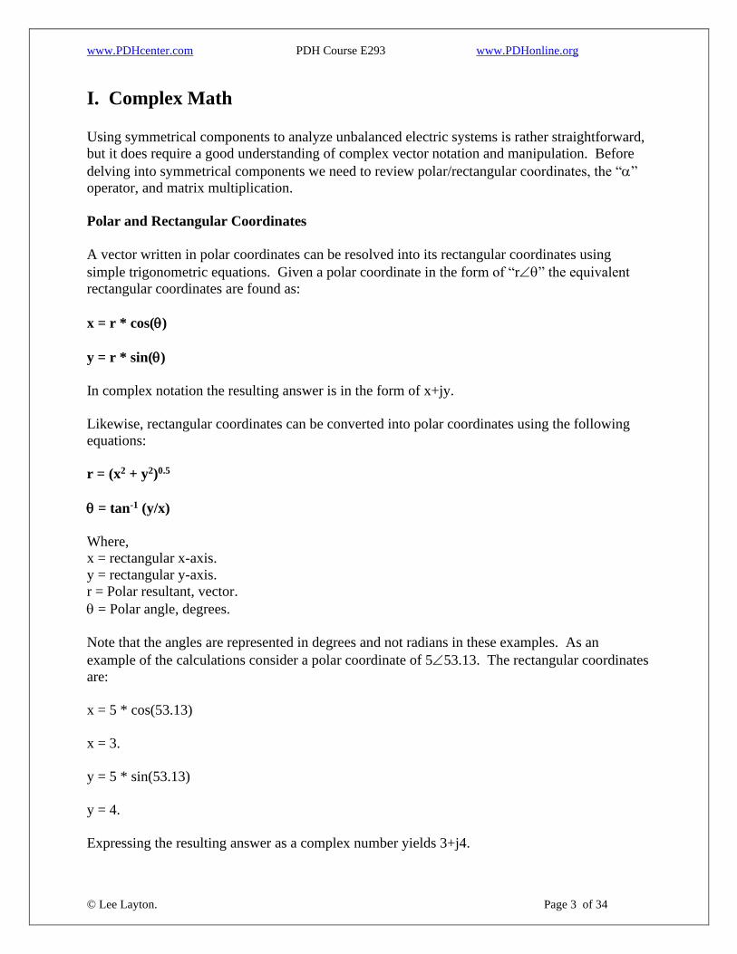
Polar and Rectangular Coordinates

A vector written in polar coordinates can be resolved into its rectangular coordinates using

simple trigonometric equations. Given a polar coordinate in the form of “r” the equivalent

rectangular coordinates are found as:

x = r * cos()

y = r * sin()

In complex notation the resulting answer is in the form of x+jy.

Likewise, rectangular coordinates can be converted into polar coordinates using the following

equations:

r = (x2 + y2)0.5

= tan-1 (y/x)

Where,

x = rectangular x-axis.

y = rectangular y-axis.

r = Polar resultant, vector.

= Polar angle, degrees.

Note that the angles are represented in degrees and not radians in these examples. As an

example of the calculations consider a polar coordinate of 553.13. The rectangular coordinates

are:

x = 5 * cos(53.13)

x = 3.

y = 5 * sin(53.13)

y = 4.

Expressing the resulting answer as a complex number yields 3+j4.





Next consider a complex number of 1+j1.732. What is the polar equivalent?

r = (12 + 1.7322)0.5

r = 2.

= tan-1(1.732/1)

= 60.

Therefore, the polar equivalent is 2

When converting from rectangular coordinates to polar

coordinates, care must be taken in deciding what angle is

being presented. Consider the figure on the left, which

shows an example of rectangular coordinates in each

quadrant. Point “B” in Figure 1 is -1+j1. Using the

formulas just presented, the polar equivalent is 1.414-

45, but the angle is referenced from the negative x-axis.

When referenced from the positive x-axis the angle is 135

degrees. Most handheld calculators will report 135

degrees for this scenario. This location can also be

referenced as -225 degrees from the x-axis. The

following table shows the results for calculations in each

of the four quadrants shown in Figure 1 along with a

typical handheld calculator results and finally the results

for angles measured from the positive x-axis in the

positive direction.

Table 1

Polar Coordinate Angle Convention Rectangular Polar Coordinates

R jX r Formula

Angle

Calculator

Angle

Positive

Convention

1 1 1.414 45 45 45

-1 1 1.414 -45 135 135

1 -1 1.414 -45 -45 315

-1 -1 1.414 45 -135 225

An easy way to resolve the angle dilemma is to add 180 degrees to the resulting polar angle if the

real component of the rectangular coordinate is negative (e.g. -1+j1, -1-j1, etc). If the imaginary

component is negative, then also add 360 degrees to the resulting polar angle.





Complex Number Multiplication

The key to complex number multiplication of rectangular coordinates is how the “j” operator is

handled. Remember that “j” is equal to the square root of a negative one, so “j2” is a negative

one.

j = sqrt(-1).

And,

j2 = -1.

Consider the following example. Multiple 3+j4 by 2+j3.

3 + j4

* 2 + j3

j + 12j2

6 + 8j .

6 + 17j + 12j2

Since j2 is equal to negative one, the equation can be simplified to,

6 + 17j + (12 * -1) or,

-6 + 17j

When multiplying polar coordinates, the resultant values are multiplied and the angle values are

added. For example, what is the product of 553.13 and 3.6156.31?

The resultant value is 5 * 3.61 or 18.05.

The angle is 53.13 + 56.31 or 109.44 degrees.

Therefore the product of 553.13 and 3.6156.31 is,

18.05 which also can be expressed in rectangular coordinates as -6+j17.

The “” Operator

The “” operator is a short-hand method of representing a phase shift difference of 120 degrees.

The “” operator has a unity value at 120 degrees or:

= 1120.

Similarly,





2 = 1 or 2 = 1−.

In rectangle coordinates the “” operator is:

= -0.5 + j0.866 and 2 = -0.5 - j0.866.

Matrices

Matrix math is a method to easily solve complex problems with multiple simultaneous equations.

A matrix is a rectangular array of numbers. The numbers can be simple or complex or a

combination.

Matrices are defined by the number of rows and columns, with the number of rows always listed

first. For instance a 2x3 matrix has two rows and three columns. Matrices are normally

identified with a capital letter such as “A”, etc. The individual numbers in the matrix are called

elements and each element can be identified by its row and column location such as “a11” for a

number in the first row and first column. Likewise “a32” is the element in row three and column

two.

All of the following are valid matrices:

The following equations:

3x + 4y = 5

3x - y = 3

Can be represented by the following matrix:





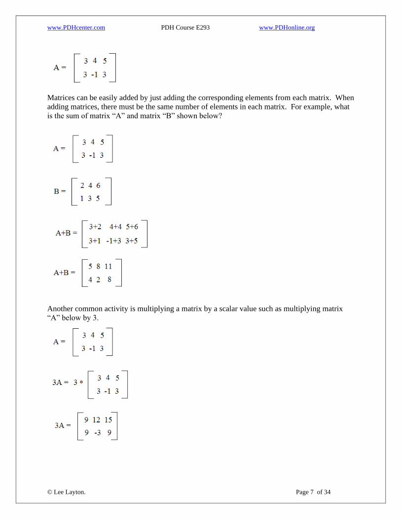
Matrices can be easily added by just adding the corresponding elements from each matrix. When

adding matrices, there must be the same number of elements in each matrix. For example, what

is the sum of matrix “A” and matrix “B” shown below?

Another common activity is multiplying a matrix by a scalar value such as multiplying matrix

“A” below by 3.





To multiply two matrices the number of rows in the first matrix must equal the number of

columns in the second matrix.

The form for multiplying a 2x1 matrix by a 1x2 matrix is:

To multiply a 2x2 by a 2x2 the form is:

As an example what is the product of matrix “A” and matrix “B” shown below?

Other size matrices can be derived from this general form.





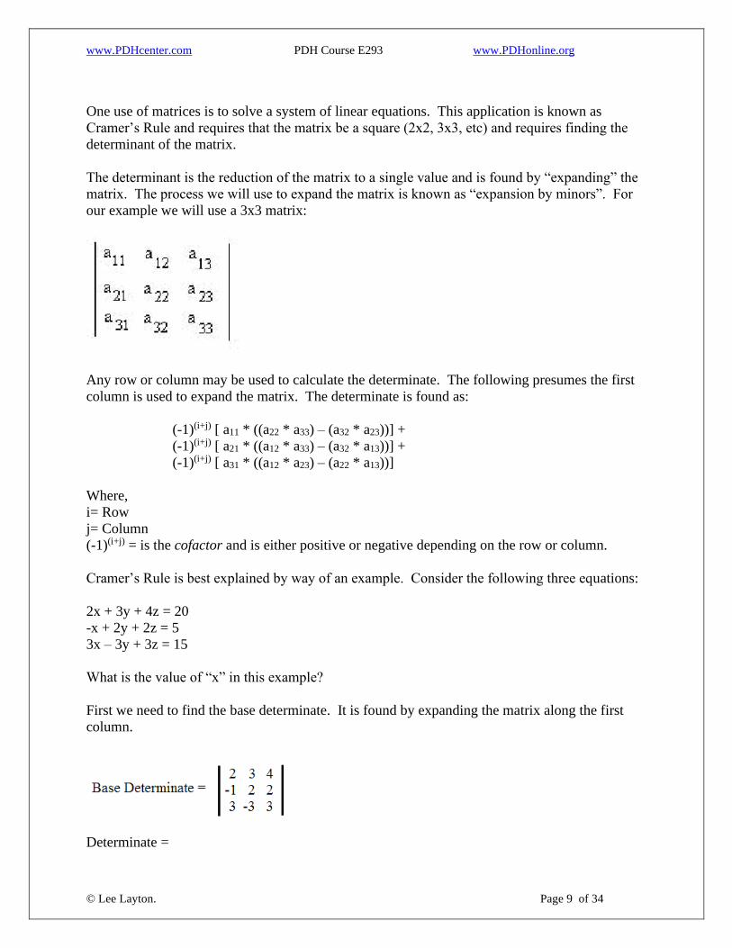
One use of matrices is to solve a system of linear equations. This application is known as

Cramer’s Rule and requires that the matrix be a square (2x2, 3x3, etc) and requires finding the

determinant of the matrix.

The determinant is the reduction of the matrix to a single value and is found by “expanding” the

matrix. The process we will use to expand the matrix is known as “expansion by minors”. For

our example we will use a 3x3 matrix:

Any row or column may be used to calculate the determinate. The following presumes the first

column is used to expand the matrix. The determinate is found as:

(-1)(i+j) [ a11 * ((a22 * a33) – (a32 * a23))] +

(-1)(i+j) [ a21 * ((a12 * a33) – (a32 * a13))] +

(-1)(i+j) [ a31 * ((a12 * a23) – (a22 * a13))]

Where,

i= Row

j= Column

(-1)(i+j) = is the cofactor and is either positive or negative depending on the row or column.

Cramer’s Rule is best explained by way of an example. Consider the following three equations:

2x + 3y + 4z = 20

-x + 2y + 2z = 5

3x – 3y + 3z = 15

What is the value of “x” in this example?

First we need to find the base determinate. It is found by expanding the matrix along the first

column.

Determinate =





1 * [ 2 * ((2 * 3) – (-3 * 2))] +

(-1) * [-1 * ((3 * 3) – (-3 * 4))] +

1 * [ 3 * ((3 * 2) – ( 2 * 4))]

Determinate = 39.

An easier method to find the determinate is to use the Excel function MDETERM. This function

will calculate the determinate of a matrix. It has the form MDETERM(A1:C3).

Once the base determinate is found, a separate determinate is found for each variable in the

equations by substituting the constants on the right-hand side of the equations for the column

where we want to solve for the variable. In our example, to solve for “x” we will substitute the

constants into the first column giving us a determinate that looks like this:

Now, finding the x-determinate:

X-determinate =

1 * [ 20 * ((2 * 3) – (-3 * 2))] +

(-1) * [ 5 * ((3 * 3) – (-3 * 4))] +

1 * [ 15 * ((3 * 2) – ( 2 * 4))]

X-determinate = 105.

The value of the variable “x” can be found by dividing the x-determinate by the base

determinate:

x = 105 / 39 = 2.69.

The variables “y” and “z” can be solved similarly.





The values for x, y, and z are:

x = 2.69

y = 0.769

z = 3.077

Next we will review the concept of sequence components and their application to electric power

systems.





II. Sequence Components

The currents (and voltages) in a normal, balanced, three-phase system are equal in magnitude

and 120 degrees apart as is shown in Figure 2. In this case, the normal rotation is assumed to be

counter-clockwise, or ABC.

However, if a single-line-to-ground fault occurs on phase “A”, the current in “A” phase will

become very large in comparison to the other phases and the phase relationship may be altered

such as is shown in Figure 3, below.





The un-symmetric and unbalanced condition shown in Figure 3 can be resolved into the balanced

conditions shown in Figure 4 by using sequence components to represent the three-phase

electrical system.

The positive sequence component of the current shown in Figure 4 is balanced in magnitude with

a 120 degree phase separation and counter-clockwise rotation, just like the original balanced

system. The negative sequence component of the current is balanced in magnitude with a 120

degree phase separation, but has the opposite rotation, in this case, clockwise. The zero

sequence components have equal magnitudes, but zero phase separation.

If you will notice in Figure 4, we have denoted the positive sequence with the subscript “1”

therefore the phase currents are labeled Ia1, Ib1, and Ic1. Likewise, the negative sequence is

denoted with the subscript “2” and the zero sequence is denoted with the subscript “0”.

Recombining the sequence components, the original currents are:

Ia = Ia0 + Ia1 + Ia2

Ib = Ib0 + I b1 + Ib2

Ic = Ic0 + Ic1 + Ic2

Since the zero sequence components are equal in magnitude with no phase separation:

Ia0 = Ib0 = Ic0

And since the positive sequence components are equal in magnitude and separated by 120

degrees, we can use the “” operator to represent the difference between phases. “C” phase is

120 degrees ahead of “A” phase so:

Ic1 = Ia1

And “B” phase lags “A” phase by 120 degrees so:

Ib1 = 2Ia1





The original phase currents can now be rewritten in terms of the “A” phase currents by using the

“” operator:

Ia = Ia0 + Ia1 + Ia2

Ib = Ia0 + 2I a1 + Ia2

Ic = Ia0 + Ia1 + 2Ia2

It is normal convention to drop the “A” phase designation from the sequence components since

each phase is referenced to the “A” phase with the “” operator, so Ia0 becomes just I0, etc. If

we factor out the sequence components into matrix form we have:

The matrix equation is sometimes written in a shorthand notation as:

Iabc = [A] I012

In the next section we will look at how to use per-unit values to simplify electric power system

calculations.





III. Per-Unit Values

Electric utility systems have many voltage and current transformations. The voltage at the

generator is stepped up to a higher voltage for transmission to the load center and then it is

stepped down to a lower voltage for distribution. A final transformation occurs as the voltage is

stepped down to usable levels for consumers. For ease of making computations it is convenient

to express system quantities in “per unit” of some base value. This allows us to model a utility

system on a common basis without regard to the changes that occur to system quantities as a

result of transformations.

The per-unit value of a quantity is defined as the ratio of the quantity to its base value expressed

as a decimal. To model a system in per-unit values, two of the four system quantities (voltage,

current, power, impedance) must be selected as the base quantities. The remaining two

quantities are then automatically fixed based on Ohm’s Law.

The most common bases for utility analysis are power and voltage, and we will use 100 MVA as

the power base and 115 kV (line-to-line voltage) as the voltage base. The voltage base for

converting to per-unit is based on the actual voltage rating at that point in the circuit; however,

the power base is constant throughout the circuit. The formulas for converting to per-unit values

are shown below.

VPU = VActual / VBase

SPU = SActual / SBase

IPU = (IActual * 1.732 * VBase) / SBase

ZPU = (ZActual * SBase) / (VBase)2

Sometimes it is necessary to convert from one base value to another. For instance, generator and

transformer impedances are usually listed as a percent of the base rating of the unit. In this case,

the per-unit impedance is found by:

ZPU New = ZPU Old * (VBase Old / VBase New)2 * (SBase New) / Sbase Old)

Where,

VPU = Voltage, per-unit.

SPU = Power, per-unit.

IPU = Current, per-unit.

ZPU = Impedance, per-unit.

VActual = Actual voltage, kilovolts.

VBase = Base voltage, 115 kV.

SActual = Actual power, Megavolt-amps (MVA).

SBase = Power base, 100 MVA.

IActual = Actual current, amps.

ZActual = Actual impedance, ohms.





ZPU Old = Impedance on original base, per-unit.

VBase Old = Original base voltage, kilovolts.

SBase Old = Original power base, MVA.

Consider the following example where a 4+j5-ohm, 115 kV transmission line is in series with a

115 kV:12.47 kV, 20 MVA transformer with an impedance of 7.5% and a 12.47 distribution line

with an impedance of 3+j6-ohms. Assuming a 115 kV voltage base and a 100 MVA power base,

what are the per-unit values for this system?

For the first transmission line the impedance is:

ZPU = (4+j5 * 100) / (115)2 = 0.0302+j0.0378

Converting to polar coordinates, the per-unit impedance is:

ZPU = 0.04851.38.

For the transformer we will assume that all of the transformer impedance is reactive. The per-

unit impedance is:

ZPU = 0.075 * (115/115)2 * (100 / 20) = j0.375.

While not actually necessary, for the second transmission line, let’s first convert the transmission

impedance into polar coordinates to simplify the calculation. For the second transmission line

the impedance is:

ZActual = 3+j6 = 6.7163.43.

ZPU = (6.7163.43 * 100) / (12.47)2 = 4.3263.43 or 1.93+j3.86.

Notice, that for the second transmission line, the voltage base is the rating of the system at this

point (12.47 kV). Once the conversion to per-unit is made, the difference in voltage levels can

be ignored in the circuit analysis.

Now that the values are converted to per-unit the circuit impedances can be simply added

together. The total circuit impedance is:

ZCircuit = 0.0302+j0.0378 + j0.375 + 1.93+j3.86 = 1.96+j4.27

Of course, after system analysis is performed using per-unit values, the values must be converted

back to actual values. The previous formulas can be re-arranged to find actual values. For

example, what is the actual value of a per-unit current of 3.58-39?

Rearranging the per-unit current formula we have:

IActual = (IPU * SBase) / (1.732 * VBase)





IActual = (3.58-39 * 100) / (1.732 * 115) * 1,000

IActual = 1,797-39 amps.

Note that since we used a 115 kV voltage base, but a 100 MVA power base, the per-unit current

value must be multiplied by 1,000 to correct for the different bases. This can be eliminated by

using the same base (i.e. use kV and kVA instead of kV and MVA.)

With an understanding of complex math, per-unit values, and system components, it is now time

to look at sequence networks.





IV. Sequence Networks

The first step in calculating sequence voltages and currents is to set up sequence networks. Each

device in a circuit can be represented by its corresponding positive, negative, and zero sequence

components. The first part of this section includes sequence schematics for typical utility

devices such as generators, transmission lines, and transformers. The second section includes

fault connection diagrams or sequence network connection diagrams.

Component Sequence Schematics

The diagram shown in Figure 5 is the sequence schematic for a generator. The zero sequence is

represented by a single impedance, X0, in series with three times the neutral impedance;

however, the neutral impedance is frequently assumed to be negligible. The positive sequence

has a voltage source (at 1.0 per unit value) in series with the positive sequence impedance. The

sub synchronous transient reactance, “Xd”, is normally for the positive sequence impedance of a

generator since it will yield the largest initial current during a fault condition. The negative

sequence impedance is the same as the positive sequence impedance. Note that the voltage

source is only in the positive sequence. The positive sequence represents the normal operating

state of the system absence a fault.





Figure 6 shows the sequence schematics for a transmission line. A transmission line naturally is

composed of series resistance and series reactance and perhaps a parallel capacitance. The series

resistance is relatively small and is usually ignored for most fault calculations as is the

capacitance, which is relatively large. The positive and negative sequence impedances are equal,

but the zero sequence will normally be a different value.





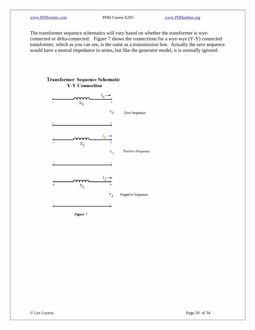
The transformer sequence schematics will vary based on whether the transformer is wye-

connected or delta-connected. Figure 7 shows the connections for a wye-wye (Y-Y) connected

transformer, which as you can see, is the same as a transmission line. Actually the zero sequence

would have a neutral impedance in series, but like the generator model, it is normally ignored.





Zero sequence currents do not flow through a delta connected transformer, and Figure 8 shows

the sequence schematic for a wye-delta transformer connection.





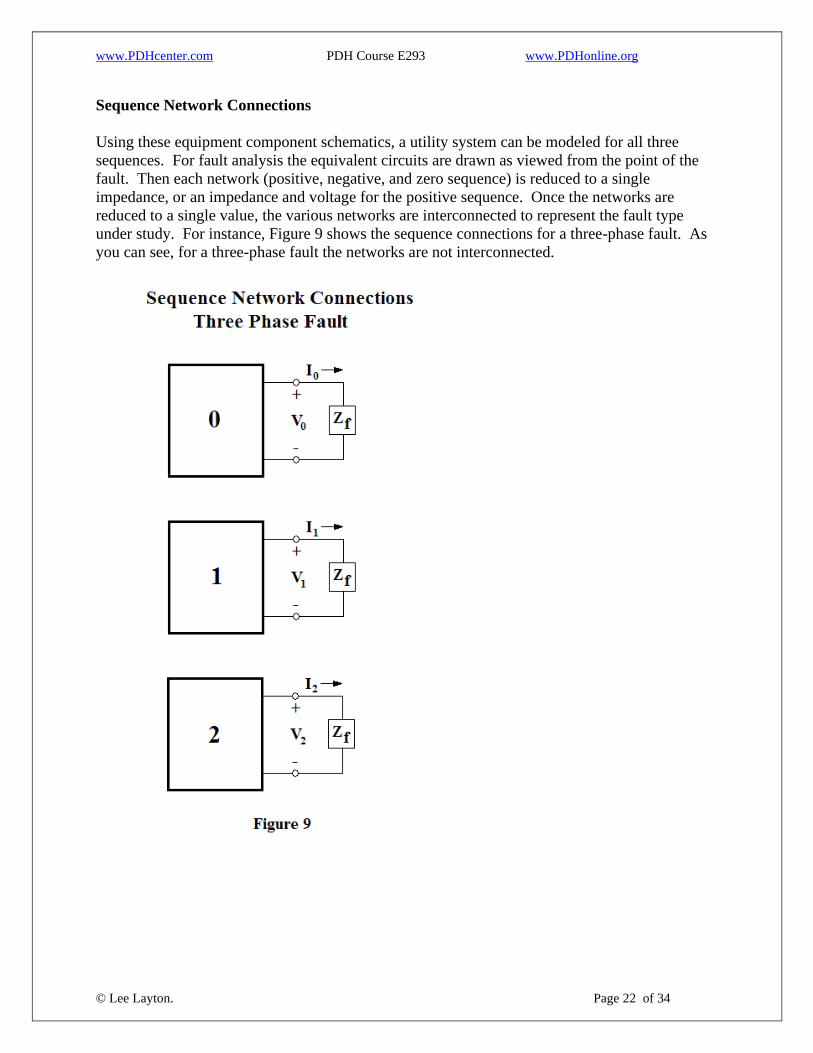
Sequence Network Connections

Using these equipment component schematics, a utility system can be modeled for all three

sequences. For fault analysis the equivalent circuits are drawn as viewed from the point of the

fault. Then each network (positive, negative, and zero sequence) is reduced to a single

impedance, or an impedance and voltage for the positive sequence. Once the networks are

reduced to a single value, the various networks are interconnected to represent the fault type

under study. For instance, Figure 9 shows the sequence connections for a three-phase fault. As

you can see, for a three-phase fault the networks are not interconnected.





In contrast to the three-phase fault shown in Figure 9, a single-line-to-ground fault is shown in

Figure 10. For a single-line-to-ground fault the networks are connected in series with the

positive sequence current flowing into the zero sequence circuit, the zero sequence flowing into

the negative sequence, and the negative sequence current flowing into the positive sequence.

The fault impedance, if any, is multiplied by three to represent the fault in all three components.





The next fault type shown is a line-to-line fault. In this case the zero sequence network is not

involved in the fault and the positive and negative sequence networks are in parallel. Figure 11

shows the line-to-line fault connection.





The final case shown is a double-line-to-ground fault, which is shown in Figure 12. In this case,

the three sequence networks are connected in parallel as opposed to the series connection of a

single-line-to-ground fault.

Sequence networks and symmetrical components are best understood by way of an example.

The next section includes an example of a faulted electrical system and the application of

symmetrical components.





VI. Example

Putting this all together, we will convert the following circuit into its respective sequence values

and schematics and solve for a fault at location “C”. The circuit consists of two generators with

step-up transformers interconnected by a 115 kV transmission line. We have assumed that the

fault occurred approximately midway between the two parallel generators. See Figure 13.

Generator #1 is a 30 MVA, 25 kV unit with a positive impedance of 22% and a zero impedance

of 8%. The voltage at generator #1 is stepped-up from 25 kV to 115 kV, using a 40 MVA wye-

wye transformer with an impedance of 15%. Generator #2 is a 40 MVA, 13.2 kV unit with a

positive impedance of 15% and a zero sequence impedance of 6%. The voltage at generator #2

is stepped-up from 13.2 kV to 115 kV with a 50 MVA delta-wye transformer with an impedance

of 8.5%. Transmission line #1 is a 115 kV line with 8-ohms of impedance and 16-ohms of zero

sequence impedance. (The impact of the line resistance is negligible in fault calculations and is

omitted for clarity here.) Transmission line #2 is a 115 kV line with 6-ohms of impedance and

15-ohms of zero sequence impedance. See Table 2 for a summary of the system parameters.

Table 2

System Parameters Component MVA Rating Voltage X1 X2 X0

Generator 1 30 MVA 25 kV 22% 22% 8%

Generator 2 40 MVA 13.2 kV 15% 15% 6%

Transformer 1 40 MVA 25:115 kV 8% 8% 8%

Transformer 2 50 MVA 13.2:115 kV 8.5% 8.5% 8.5%

Line 1 - 115 kV 0+j8 0.+j8 0+j16

Line 2 - 115 kV 0+j6 0+j6 0+j15

We will use the following steps to analyze the fault problem.

1. Determine the component impedances and convert to per unit values on a common base.

2. Draw positive, negative, and zero sequence circuits.

3. Reduce the circuits to single impedance equivalent circuits.

4. Connect equivalent circuits for the fault type under study.

5. Analyze the fault.





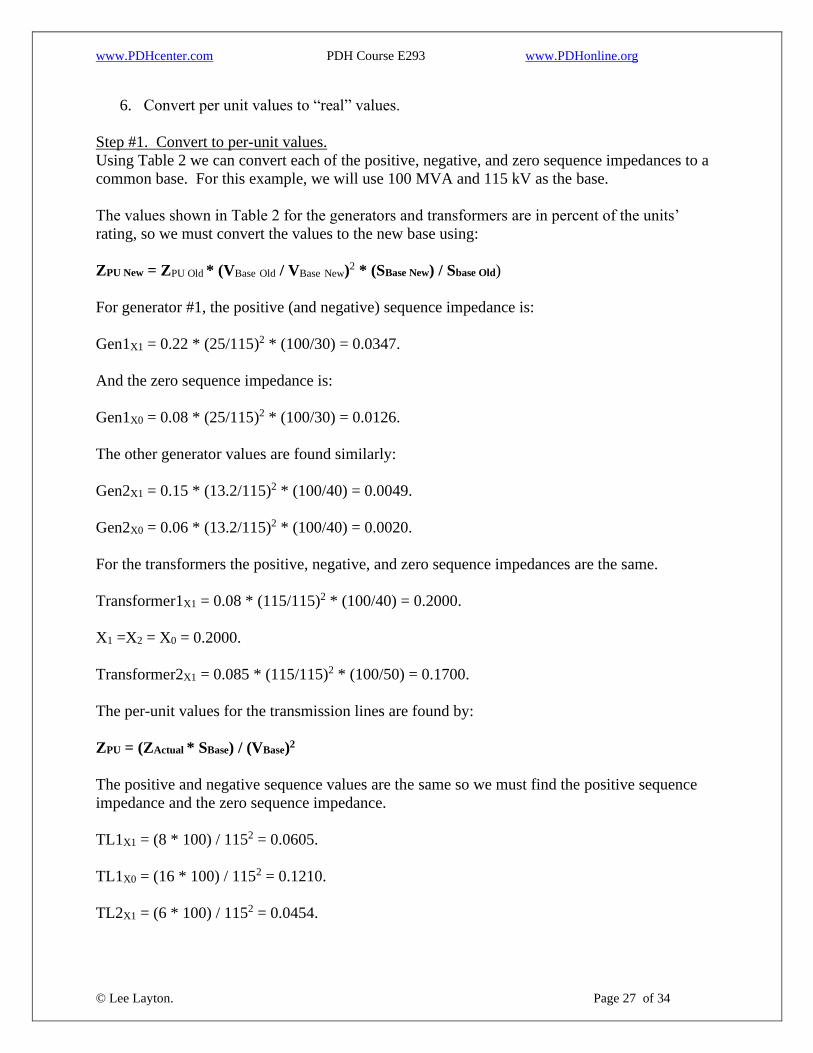
6. Convert per unit values to “real” values.

Step #1. Convert to per-unit values.

Using Table 2 we can convert each of the positive, negative, and zero sequence impedances to a

common base. For this example, we will use 100 MVA and 115 kV as the base.

The values shown in Table 2 for the generators and transformers are in percent of the units’

rating, so we must convert the values to the new base using:

ZPU New = ZPU Old * (VBase Old / VBase New)2 * (SBase New) / Sbase Old)

For generator #1, the positive (and negative) sequence impedance is:

Gen1X1 = 0.22 * (25/115)2 * (100/30) = 0.0347.

And the zero sequence impedance is:

Gen1X0 = 0.08 * (25/115)2 * (100/30) = 0.0126.

The other generator values are found similarly:

Gen2X1 = 0.15 * (13.2/115)2 * (100/40) = 0.0049.

Gen2X0 = 0.06 * (13.2/115)2 * (100/40) = 0.0020.

For the transformers the positive, negative, and zero sequence impedances are the same.

Transformer1X1 = 0.08 * (115/115)2 * (100/40) = 0.2000.

X1 =X2 = X0 = 0.2000.

Transformer2X1 = 0.085 * (115/115)2 * (100/50) = 0.1700.

The per-unit values for the transmission lines are found by:

ZPU = (ZActual * SBase) / (VBase)2

The positive and negative sequence values are the same so we must find the positive sequence

impedance and the zero sequence impedance.

TL1X1 = (8 * 100) / 1152 = 0.0605.

TL1X0 = (16 * 100) / 1152 = 0.1210.

TL2X1 = (6 * 100) / 1152 = 0.0454.





TL2X0 = (15 * 100) / 1152 = 0.1134.

Step #2. Draw the positive, negative, and zero sequence circuits.

Using the circuit shown in Figure 13, we can draw positive, negative, and zero sequence circuits

as shown in the following figures. Figure 14 is a positive sequence schematic of the two source

utility model shown in Figure 13. The individual components are connected based on the

diagrams shown previously in Section IV.

Figure 15 shows the negative sequence schematic, which is the same as the positive sequence

schematic except that the voltage sources are not present. Voltages sources are only shown in

the positive sequence circuit except for some motor devices.

Figure 16 is the zero sequence schematic. Like the negative sequence circuit, this circuit does

not have voltage sources. Notice that since transformer #2, which is connected between nodes

“D” and “E”, is connected wye-delta the zero sequence currents cannot flow from generator #2

to the fault at node “C”.





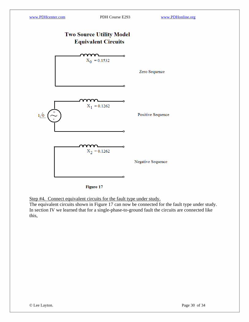
Step #3. Reduce the circuits to single impedance equivalent circuits.

The circuits presented in Step #2 are now reduced to single impedance (and in the case of the

positive sequence, single voltage) equivalent circuits using standard circuit reduction techniques.

This results in a positive sequence impedance of 0.1262, a negative sequence impedance of

0.1262, and a zero sequence impedance of 0.1532. Figure 17 shows the resulting circuits.





Step #4. Connect equivalent circuits for the fault type under study.

The equivalent circuits shown in Figure 17 can now be connected for the fault type under study.

In section IV we learned that for a single-phase-to-ground fault the circuits are connected like

this,





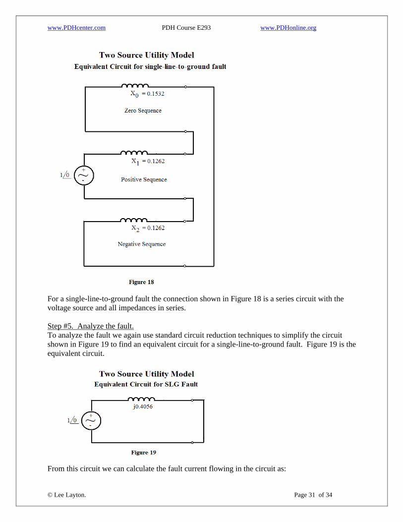
For a single-line-to-ground fault the connection shown in Figure 18 is a series circuit with the

voltage source and all impedances in series.

Step #5. Analyze the fault.

To analyze the fault we again use standard circuit reduction techniques to simplify the circuit

shown in Figure 19 to find an equivalent circuit for a single-line-to-ground fault. Figure 19 is the

equivalent circuit.

From this circuit we can calculate the fault current flowing in the circuit as:





I = (10) / (0+j0.4056) = -j2.4655.

Because the single-line-to-ground fault circuit is a series circuit, I1 = I2 = I0. With the currents

known, the sequence voltages can easily be found.

V0 = (-j0.1532) * (-j2.4655) = -0.3777

V1 = 10 + (-j0.1262)*(-j2.4655) = 0.6889

V2 = (-j0.1262) * (-j2.4655) = -0.3111

The phase currents and voltages can now be found using the sequence component matrix.

Since we know that all of the sequence currents are –j2.4655 the phase currents are:

Ia = (1 * -j2.4655) + (1 * -j2.4655) + (1 * -j2.4655) = 0-j7.397

Ib = (1 * -j2.4655) + (1240 * -j2.4655) + (1120 * -j2.4655) = 0+j0

Ic = (1 * -j2.4655) + (1 * -j2.4655) + (1 * -j2.4655) = 0+j0

These values are what you would expect because the fault is in Phase “A”, and no significant

current is flowing in the other phases.

The phase voltages are found in a similar fashion.

We found the sequence voltages to be V0 =-0.3777, V1 = 0.6889, V2 = -0.3111. The phase

voltages are:

Va = (1 * -0.3777) + (1 * 0.6889) + (1 * -0.3111) = 0

Vb = (1 * -0.3777) + (1240 * 0.6889) + (1120 * -0.3111) = 1.035237

Vc = (1 * -0.3777) + (1 * 0.6889) + (1 * -0.3111) = 1.035123





Again, this is what you would expect, the “A” phase voltage has collapsed due to the fault and

the remaining phases have become asymmetrical due to the fault condition.

Step #6. Convert per unit values to “real” values.

The final step is to convert the phase voltages and currents into actual values.

Rearranging the formulas from Section III we can find the actual voltages and currents as:

IActual = (IPU * SBase)/ (1.732 * VBase)

VActual = VPU * VBase

Ia = (−j ) ( ) = -90 amps.

(Remember to multiply the currents by 1,000 because of the difference in the voltage and power

bases.

As previously mentioned, Ib = Ic = 0 amps.

Va = 0 Volts.

Vb = 1.035237 * 115 = 119.0237 kV.

Vc = 1.035123 * 115 = 119.0123 kV.

Other types of faults such as double-line-to-ground and line-to-line faults can be worked using

these same steps by using the appropriate network connections and reducing the circuits to an

equivalent voltage and impedance. The circuit diagram set up in this example is only valid for a

fault at location “C”. For faults at other locations, the circuit diagrams will need to be redrawn.





Summary

The application of symmetrical components takes an unbalanced network of three related vectors

and resolves them into three sets of vectors. Two of these sets have equal magnitude and are

displaced 120 degrees apart while the third set has equal magnitude, but zero phase

displacement. To use symmetrical components we must know the sequence network

connections for various fault types and sequence connections for different components.

Applying the concepts of symmetrical components to three-phase electric power networks makes

the analysis of unbalanced conditions manageable. Even with symmetrical component analysis,

the application can be tedious and most engineers use sophisticated computer systems to model

unbalanced conditions. It is worthwhile though, to understand how symmetrical components are

used to analyze electric systems.

Copyright © 2006 Lee Layton. All Rights Reserved.

+++



Symmetrical Components Application to Electric …Symmetrical Components Application to Electric...

Documents

Transcript of Symmetrical Components Application to Electric …Symmetrical Components Application to Electric...