Symmetric Non-Rigid Structure from Motion for …alanlab/Pubs16/gao2016symmetric.pdf · Symmetric...
20
Symmetric Non-Rigid Structure from Motion for Category-Specific Object Structure Estimation Yuan Gao 1? and Alan L. Yuille 2,3 1 City University of Hong Kong 2 UCLA 3 Johns Hopkins University {Ethan.Y.Gao, Alan.L.Yuille}@gmail.com Abstract. Many objects, especially these made by humans, are sym- metric, e.g. cars and aeroplanes. This paper addresses the estimation of 3D structures of symmetric objects from multiple images of the same object category, e.g. different cars, seen from various viewpoints. We as- sume that the deformation between different instances from the same object category is non-rigid and symmetric. In this paper, we extend two leading non-rigid structure from motion (SfM) algorithms to exploit symmetry constraints. We model the both methods as energy minimiza- tion, in which we also recover the missing observations caused by occlu- sions. In particularly, we show that by rotating the coordinate system, the energy can be decoupled into two independent terms, which still ex- ploit symmetry, to apply matrix factorization separately on each of them for initialization. The results on the Pascal3D+ dataset show that our methods significantly improve performance over baseline methods. Keywords: Symmetry, Non-Rigid Structure from Motion 1 Introduction 3D structure reconstruction is a major task in computer vision. Structure from motion (SfM) method, which aims at estimating the 3D structure by the 2D annotated keypoints from 2D image sequences, has been proposed for rigid ob- jects [1], and was later extended to non-rigidity [2–14]. Many man-made objects have symmetric structures [15, 16]. Motivated by this, symmetry has been stud- ied extensively in the past decades [16–22]. However, this information has not been exploited in recent works on 3D object reconstruction [23, 24], nor used in standard non-rigid structure from motion (NRSfM) algorithms [3–10, 14]. The goal of this paper is to investigate how symmetry can improve NRSfM. Inspired by recent works [23, 24], we are interested in estimating the 3D structure of objects, such as cars, airplanes, etc. This differs from the classic SfM problem because our input are images of several different object instances from the same category (e.g. different cars), instead of sequential images of the same object undergoing motion. In other words, our goal is to estimate the 3D structures of objects from the same class, given intra-class instances from various viewpoints. ? This work was been done when Yuan Gao was a visiting student in UCLA.
Transcript of Symmetric Non-Rigid Structure from Motion for …alanlab/Pubs16/gao2016symmetric.pdf · Symmetric...

Symmetric Non-Rigid Structure from Motion forCategory-Specific Object Structure Estimation
Yuan Gao1? and Alan L. Yuille2,3
1 City University of Hong Kong 2 UCLA 3 Johns Hopkins University{Ethan.Y.Gao, Alan.L.Yuille}@gmail.com
Abstract. Many objects, especially these made by humans, are sym-metric, e.g. cars and aeroplanes. This paper addresses the estimation of3D structures of symmetric objects from multiple images of the sameobject category, e.g. different cars, seen from various viewpoints. We as-sume that the deformation between different instances from the sameobject category is non-rigid and symmetric. In this paper, we extendtwo leading non-rigid structure from motion (SfM) algorithms to exploitsymmetry constraints. We model the both methods as energy minimiza-tion, in which we also recover the missing observations caused by occlu-sions. In particularly, we show that by rotating the coordinate system,the energy can be decoupled into two independent terms, which still ex-ploit symmetry, to apply matrix factorization separately on each of themfor initialization. The results on the Pascal3D+ dataset show that ourmethods significantly improve performance over baseline methods.
Keywords: Symmetry, Non-Rigid Structure from Motion
1 Introduction
3D structure reconstruction is a major task in computer vision. Structure frommotion (SfM) method, which aims at estimating the 3D structure by the 2Dannotated keypoints from 2D image sequences, has been proposed for rigid ob-jects [1], and was later extended to non-rigidity [2–14]. Many man-made objectshave symmetric structures [15,16]. Motivated by this, symmetry has been stud-ied extensively in the past decades [16–22]. However, this information has notbeen exploited in recent works on 3D object reconstruction [23,24], nor used instandard non-rigid structure from motion (NRSfM) algorithms [3–10,14].
The goal of this paper is to investigate how symmetry can improve NRSfM.Inspired by recent works [23,24], we are interested in estimating the 3D structureof objects, such as cars, airplanes, etc. This differs from the classic SfM problembecause our input are images of several different object instances from the samecategory (e.g. different cars), instead of sequential images of the same objectundergoing motion. In other words, our goal is to estimate the 3D structures ofobjects from the same class, given intra-class instances from various viewpoints.
? This work was been done when Yuan Gao was a visiting student in UCLA.

2 Y. Gao and A. Yuille
Specifically, the Pascal3D+ keypoint annotations on different objects from thesame category are used as input to our method, where the the symmetric key-point pairs can also be easily inferred. In this paper, non-rigidity means thedeformation between the objects from same category can be non-rigid, e.g. be-tween sedan and SUV cars, but the objects themselves are rigid and symmetric.
By exploiting symmetry, we propose two symmetric NRSfM methods. Byassuming that the 3D structure can be represented by a linear combinationof basis functions (the coefficients vary for different objects): one method isan extension of [5] which is based on an EM approach with a Gaussian prioron the coefficients of the deformation bases, named Sym-EM-PPCA; the othermethod, i.e. Sym-PriorFree, is an extension of [9, 10], which is a direct matrixfactorization method without prior knowledge. For fair comparison, we use thesame projection models and other assumptions used in [5] and [9,10].
More specifically, our Sym-EM-PPCA method, following [5], assumes weakperspective projection (i.e. the orthographic projection plus scale). We group thekeypoints into symmetric keypoint pairs. We assume that the 3D structure isalso symmetric and consists of a mean shape (of that category) and a linear com-bination of the symmetric deformation bases. As in [5], we put a Gaussian prioron the coefficient of the deformation bases. This is intended partly to regularizethe problem and partly to deal an apparent ambiguity in non-rigid structurefrom motion. But recent work [25] showed that this is a “gauge freedom” whichdoes not affect the estimation of 3D structure, so the prior is not really needed.
Our Sym-PriorFree method is based on prior free non-rigid SfM algorithms[9, 10], which build on the insights in [25]. We formulate the problem of esti-mating 3D structure and camera parameters in terms of minimizing an energyfunction, which exploits symmetry, and at the same time can be re-expressed asthe sum of two independent energy functions. Each of these energy functions canbe minimized separately by matrix factorization, similar to the methods in [9,10],and the ambiguities are resolved using orthonormality constraints on the view-point parameters. This extends work in a companion paper [26], which showshow symmetry can be used to improve rigid structure from motion methods [1].
Our main contributions are: (I) Sym-EM-PPCA, which imposes symmetricconstraints on both 3D structure and deformation bases. Sym-Rigid-SfM (see ourcompanion paper [26]) is used to initialize Sym-EM-PPCA with hard symmetricconstraints on the 3D structure. (II) Sym-PriorFree, which extends the matrixfactorization methods of [9, 10], to initialize a coordinate descent algorithm.
In this paper, we group keypoints into symmetric keypoint pairs, and use asuperscript † to denote symmetry, i.e. Y and Y † are the 2D symmetric keypointpairs. The paper is organized as follows: firstly, we review related works in Section2. In Section 3, the ambiguities in non-rigid SfM are discussed. Then we presentthe Sym-EM-PPCA algorithm and Sym-PriorFree algorithm in Section 4. Afterthat, following the experimental settings in [24], we evaluated our methods onthe Pascal3D+ dataset [27] in Section 5. Section 5 also includes diagnostic resultson the noisy 2D annotations to show that our methods are robust to imperfectsymmetric annotations. Finally, we give our conclusions in Section 6.
Symmetric NRSfM for Category-Specific Object Structure Estimation 3
2 Related Works
There is a long history of using symmetry as a cue for computer vision tasks.For example, symmetry has been used in depth recovery [17, 18, 20] as well asrecognizing symmetric objects [19]. Several geometric clues, including symmetry,planarity, orthogonality and parallelism have been taken into account for 3Dscene reconstruction [28, 29], in which the author used pre-computed camerarotation matrix by vanishing point [30]. Recently, symmetry has been appliedin more areas such as 3D mesh reconstruction with occlusion [21], and scenereconstruction [16]. For 3D keypoints reconstruction, symmetry, incorporatedwith planarity and compactness prior, has also been studied in [22].
SfM has also been studied extensively in the past decades, ever since theseminal work on rigid SfM [1, 31]. Bregler et al. extended this to the non-rigidcase [32]. A Column Space Fitting (CSF) method was proposed for rank-r matrixfactorization (MF) for SfM with smooth time-trajectories assumption [7], whichwas later unified in a more general MF framework [33]1. Early analysis of NRSfMshowed that there were ambiguities in 3D structure reconstruction [4]. This leadto studies which assumed priors on the NR deformations [4–7, 34, 35]. But itwas then shown that these ambiguities did not affect the final estimate of 3Dstructure, i.e. all legitimate solutions lying in the same subspace (despite under-constrained) give the same solutions for the 3D structure [25]. This facilitated theinvention of prior free matrix factorization method for NRSfM [9, 10]. RecentlySfM methods have also been used for category-specific object reconstruction,e.g. estimating the shape of different cars under various viewing conditions [23,24], but the symmetry cues was not exploited. Note that repetition patternshave recently been incorporated into SfM for urban facades reconstruction [36],but this mainly focused on repetition detection and registration. Finally, in acompanion paper [26], we exploited symmetry for rigid SfM.
3 The Ambiguities in Non-rigid SfM
This section reviews the intrinsic ambiguities in non-rigid SfM, i.e. (i) the ambi-guities between the camera projection and the 3D structure, and (ii) the ambi-guities between the deformation bases and their coefficients [25]. In the followingsections (i.e. in Remark 5), we will show the ambiguity between camera projec-tion and 3D structure (i.e. originally the 3 × 3 matrix ambiguity as discussedbelow) can be decomposed into two types of ambiguities under the symmetricconstraints, i.e. a scale ambiguity along the symmetry axis, and a 2× 2 matrixambiguity on the other two axes.
The key idea of non-rigid SfM is to represent the non-rigid deformations ofobjects in terms of a linear combination of bases:
Y = RS and S = Vz, RRT = I, (1)
1 However, the general framework in [33] cannot be used to SfM directly, because theydid not constrain that all the keypoints have the same translation.

4 Y. Gao and A. Yuille
where Y is the stacked 2D keypoints, R is the camera projection for the Nimages. S is the 3D structure which is modeled by the linear combination of thestacked deformation bases V, and z is the coefficient.
Firstly, as is well known, there are ambiguities between the projection Rand the 3D structure S in the matrix factorization, i.e. let A1 be an invertiblematrix, then R← RA1 and S← A−11 S will not change the value of RS. Theseambiguities can be solved by imposing orthogonality constraints on the cameraparameters RRT = I up to a fixed rotation, which is a “gauge freedom” [37]corresponding to a choice of coordinate system.
In addition, there are other ambiguities between the coefficients z and thedeformation bases V [4]. Specifically, let A2 be another invertible matrix, andlet w lie in the null space of the projected deformation bases RV, then z← A2zand V ← VA−12 , or z ← z + αw will not change the value of RVz. This moti-vated Bregeler et al. to impose a Gaussian prior on the coefficient z in order toeliminate the ambiguities. Recently, it was proved in [25] that these ambiguitiesare also “fake”, i.e. they do not affect the estimate of the 3D structure. Thisproof facilitated prior-free matrix factorization methods for non-rigid SfM [9,10].
4 Symmetric Non-Rigid Structure from Motion
In this paper we extend non-rigid SfM methods by requiring that the 3D struc-ture is symmetric. We assume the deformations are non-rigid and also symmet-ric2. We propose two symmetric non-rigid SfM models. One is the extension ofthe iterative EM-PPCA model with a prior on the deformation coefficients [5],and the other extends the prior-free matrix factorization model [9, 10].
For simplicity of derivation, we focus on estimating the 3D structure andcamera parameters. In practice, there are occluded keypoints in almost all imagesin the Pascal3D+ dataset. But we use standard ways to deal with them, such asinitializing them ignoring symmetry by rank 3 recovery using the first 3 largestsingular value, then treating them as missing data to be estimated by EM orcoordinate descent algorithms. In our companion paper [26], we gave details ofthese methods for the simpler case of rigid structure from motion.
Note that we use slightly different camera models for Sym-EM-PPCA (weakperspective projection) and Sym-PriorFree (orthographic projection). This is tostay consistent with the non-symmetric methods which we compare with, namely[5] and [9, 10]. Similarly, we treat translation differently by either centeralizingthe data or treating it as a variable to be estimated, as appropriate. We willdiscuss this further when presenting the Sym-PriorFree method.
4.1 The Symmetric EM-PPCA Model
In EM-PPCA [5], Bregler et al. assume that the 3D structure is represented bya mean structure S plus a non-rigid deformation. Suppose there are P keypoints
2 We assume symmetric deformations because our problem involves deformations fromone symmetric object to another. But it also can be extended to non-symmetricdeformations straightforwardly.

Symmetric NRSfM for Category-Specific Object Structure Estimation 5
on the structure, the non-rigid model of EM-PPCA is:
Yn = Gn(S + Vzn) + Tn +Nn, (2)
where Yn ∈ R2P×1, S ∈ R3P×1, and Tn ∈ R2P×1 are the stacked vectors of 2Dkeypoints, 3D mean structure and translations. Gn = IP ⊗ cnRn, in which cn isthe scale parameter for weak perspective projection, V = [V1, ...,VK ] ∈ R3P×K
is the grouped K deformation bases, zn ∈ RK×1 is the coefficient of the K bases,and Nn is the Gaussian noise Nn ∼ N (0, σ2I).
Extending Eq. (2) to our symmetry problem in which there are P keypointpairs Yn and Y†n, we have:
Yn = Gn(S + Vzn) + Tn +Nn, Y†n = Gn(S† + V†zn) + Tn +Nn. (3)
Assuming that the object is symmetric along the x-axis, the relationshipbetween S and S†, V and V† are:
S† = AP S, V† = APV, (4)
where AP = IP ⊗A, A = diag([−1, 1, 1]) is a matrix operator which negates thefirst row, and IP ∈ RP×P is an identity matrix. Thus, we have3:
P (Yn|zn, Gn, S,V,T) = N (Gn(S + Vzn) + Tn, σ2I)
P (Y†n|zn, Gn, S,V†,T) = N (Gn(AP S + V†zn) + Tn, σ2I) (5)
Following Bregler et al. [5], we introduce a prior P (zn) on the coefficientvariable zn. This prior is a zero mean unit variance Gaussian. It is used for(partly) regularizing the inference task but also for dealing with the ambiguitiesbetween basis coefficients zn and bases V, as mentioned above (when [5] waspublished it was not realized that these are “gauge freedom”). This enables usto treat zn as the hidden variable and use EM algorithm to estimate the structureand camera viewpoint parameters. The formulation of the problem, in terms ofGaussian distributions (or, more technically, the use of conjugate priors) meansthat both steps of the EM algorithm are straightforward to implement.
Remark 1. Our Sym-EM-PPCA method is a natural extension of the methodin [5] to maximize the marginal probability P (Yn,Y†n|Gn, S,V,V†,T) with aGaussian prior on zn and a Language multiplier term (i.e. a regularization term)on V,V†. This can be solved by general EM algorithm [38], where both the Eand M steps take simple forms because the underlying probability distributionsare Gaussians (due to conjugate Gaussian prior).
E-Step: This step is to get the statistics of zn from its posterior. Let the prioron zn be P (zn) = N (0, I) as in [5]. Then, we have P (zn), P (Yn|zn;σ2, S,V, Gn,Tn)
3 We set hard constraints on S and S†, i.e. replace S† by AP S in Eq. (5), because it canbe guaranteed by the Sym-RSfM initialization in our companion paper [26]. Whilethe initialization on V and V† by PCA cannot guarantee such a desirable property,thus a Language multiplier term is used for the constraint on V and V† in Eq. (9).
6 Y. Gao and A. Yuille
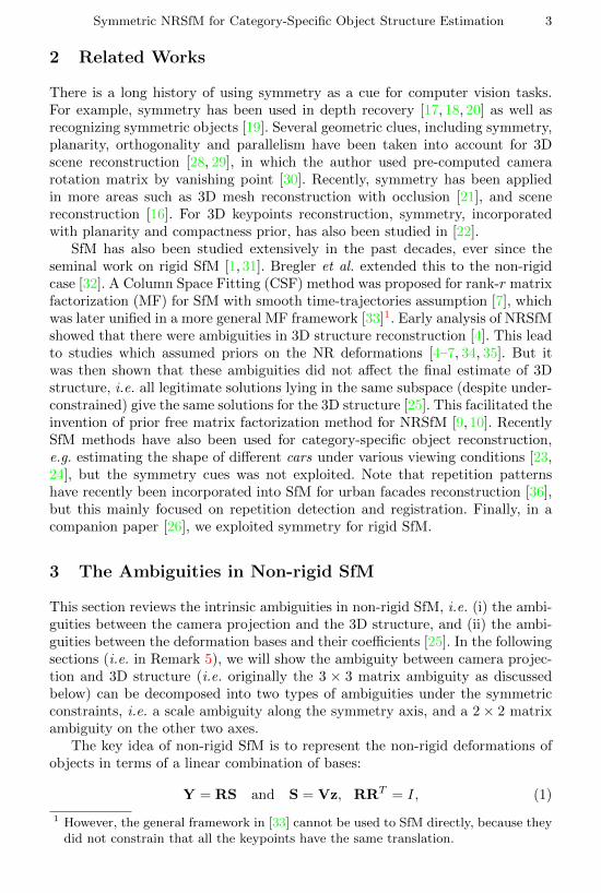
Fig. 1. The graphical model of the variables and parameters.
and P (Y†n|zn;σ2, S,V†, Gn,Tn), which do not provide the complete posterior dis-tribution directly. Fortunately, the conditional dependence of the variables shownin Fig. 1 (graphical model) implies that the posterior of zn can be calculated by:
P (zn|Yn,Y†n;σ2, S,V,V†, Gn,Tn)
∼P (zn,Yn,Y†n|σ2, S,V,V†, Gn,Tn)
=P (Yn|zn;σ2, S,V, Gn,Tn)P (Y†n|zn;σ2, S,V†, Gn,Tn)P (zn)
=N (zn|µn, Σn) (6)
The last equation of Eq. (6) is obtained by the fact that the prior and theconditional distributions of zn are all Gaussians (conjugate prior). Then thefirst and second order statistics of zn can be obtained as:
µn = γ{VTGTn (Yn −GnS− Tn) + V†TGTn (Y†n −GnAP S− Tn)
}(7)
φn = σ2γ−1 + µnµTn (8)
where γ = (VTGTnGnV + V†TGTnGnV† + σ2I)−1.M-Step: This is to maximize the joint likelihood which is similar to the
coordinate descent in Sym-RSfM (in a companion paper [26]) and that in Sym-PriorFree method in the later sections. The complete log-likelihood Q(θ) is:
Q(θ) =−∑n
lnP (Yn,Y†n|zn;Gn, S,V,V†,T) + λ||V† −APV||2
=−∑n
(lnP (Yn|zn;Gn, S,V,T) + lnP (Y†
n|zn;Gn, S,V†,T))
+ λ||V† −APV||2
s. t. RnRTn = I, where θ = {Gn, S,V,V†,Tn, σ
2}. (9)
The maximization of Eq. (9) is straightforward, i.e. taking the derivativeof each unknown parameter in θ and equating it to 0. The update rule of eachparameter is very similar to the original EM-PPCA [5] (except S,V,V† shouldbe updated jointly), which we put in Appendix A2.
Initialization. V and V† are initialized by the PCA on the residual of the2D keypoints minus their rigid projections iteratively. Other variables (includingthe rigid projections) are initialized by Sym-RSfM [26]. Specifically, Rn, S andthe occluded points Yn,p, Y
†n,p can be initialized directly from Sym-RSfM, cn is
initialized as 1, tn is initialized by tn =∑p(Yn,p −RnSp + Y †n,p −RnASp).
4.2 The Symmetric Prior-Free Matrix Factorization Model
In the Prior-Free NRSfM [9, 10], Dai et al. also used the linear combination ofseveral deformations bases to represent the non-rigid deformation. But, unlike

Symmetric NRSfM for Category-Specific Object Structure Estimation 7
EM-PPCA [5], Dai et al. estimated the non-rigid structure directly withoutusing the mean structure and the prior on the coefficients. We make the sameassumptions so that we can directly compare with them.
Assume that Yn ∈ R2×P are the P keypoints for image n, then we have:
Yn = RnSn = [zn1Rn, ..., znKRn][V1, ...,VK ]T = ΠnV,
Y †n = RnS†n = [zn1Rn, ..., znKRn][V†1, ...,V
†K ]T = ΠnV†, (10)
where zn = [zn1, ..., znK ] ∈ R1×K , Πn = Rn(zn ⊗ I3) ∈ R2×3K , and V =[VT
1 , ...,VTK ]T ∈ R3K×P .
Without loss of generality, we assume that the symmetry is across the x-axis:Sn = AS†n, where A = diag[−1, 1, 1]T is a matrix operator negating the first rowof Sn. Then the first two terms in Eq. (10) give us the energy function (or thelikelihood) to estimate the unknown Rn, Sn and recover the missing data bycoordinate descent on:
Q(Rn, Sn, {Yn,p, (n, p) ∈ IVS}, {Y †n,p, (n, p) ∈ IVS †})
=∑
(n,p)∈VS
||Yn,p −RnSn,p||22 +∑
(n,p)∈VS†
||Y †n,p −RnASn,p||22+
∑(n,p)∈IVS
||Yn,p −RnSn,p||22 +∑
(n,p)∈IVS†
||Y †n,p −RnASn,p||22, (11)
where V S and IV S are the index sets of the visible and invisible keypoints, re-spectively. Yn,p and Sn,p are the 2D and 3D p’th keypoints of the n’th image. We
treat the {Yn,p, (n, p) ∈ IVS}, {Y †n,p, (n, p) ∈ IVS †} as missing/hidden variablesto be estimated.
Remark 2. It is straightforward to minimize Eq. (11) by coordinate descent. Themissing points can be initialized simply by rank 3 recovery (i.e. by the recon-struction using the first 3 largest singular value) ignoring the symmetry propertyand non-rigidity. But it is much harder to get good initializations for the Rn andSn. In the following, we will describe how we get good initializations for eachRn and Sn exploiting symmetry after the missing points have been initialized.
Let Y is the stacked keypoints of N images, Y = [Y T1 , ..., YTN ]T ∈ R2N×P ,
the model is represented by:
Y = RS =
R1S1
...RNSN
=
z11R1, ..., z1KR1
.... . .
...zN1RN , ..., zNKRN
V1
...VK
= ΠV, (12)
where R = blkdiag([R1, ..., RN ]) ∈ R2N×3N are the stacked camera projectionmatrices, in which blkdiag denotes block diagonal. S = [ST1 , ..., S
TN ]T ∈ R3N×P
are the stacked 3D structures. Π = R(z⊗ I3) ∈ R2N×3K , where z ∈ RN×K arethe stacked coefficients. Similar equations apply to Y†.

8 Y. Gao and A. Yuille
Note that R ∈ R2N×3N , V ∈ R3K×P are stacked differently than how theywere stacked for the Sym-EM-PPCA method (i.e. R ∈ R2N×3, V ∈ R3P×K). Itis because now we have N different Sn’s (i.e. S ∈ R3N×P ), while there is onlyone S in the Sym-EM-PPCA method.
In the following, we assume the deformation bases are symmetric, which en-sures that the non-rigid structures are symmetric (e.g. the deformation fromsedan to truck is non-rigid and symmetric since sedan and truck are both sym-metric). This yields an energy function:
Q(R,S) =||Y −RS||22 + ||Y† −RANS†||22=||Y −ΠV||22 + ||Y† −ΠAKV†||22, (13)
where AN = IN ⊗A,AK = IK ⊗A, and A = diag([−1, 1, 1]).
Remark 3. Note that we cannot use the first equation of Eq. (13) to solveR,S directly (even if not exploiting symmetry), because Y and Y† are of rankmin{2N, 3K,P} but estimating R,S directly by SVD on Y and/or Y† requiresrank 3N matrix factorization. Hence we focus on the last equation of Eq. (13) toget the initialization of Π,V firstly. Then, R,S can be updated by coordinatedescent on the first equation of Eq. (13) under orthogonality constraints on Rand low-rank constraint on S.
Observe that the last equation of Eq. (13) cannot be optimized directly bySVD either, because they consist of two terms which are not independent. Inother words, the matrix factorizations of Y and Y† do not give consistent estima-tions of Π and V. Instead, we now discuss how to estimate Π and V by rotatingthe coordinate axes (to decouple the depended energy terms), performing ma-trix factorization, and using subspace intersection (to eliminate the ambiguities),which is an extension of the original prior-free method [9,10] and our companionSym-RSfM [26].
We first rotate coordinate systems (of Y,Y†) to obtain decoupled equations:
L =Y −Y†
2= Π1Vx M =
Y + Y†
2= Π2Vyz, (14)
where the two righthand sides of the equation depend on different components ofΠ, V. More specifically, by discarding the all 0 rows of the bases, Π1 ∈ R2N×K ,Π2 ∈ R2N×2K , Vx ∈ RK×P , Vyz ∈ R2K×P .
This yield two independent energies to be minimized separately by SVD:
Q(Π,V) = ||L− Π1Vx||22 + ||M− Π2Vyz||22 (15)
Remark 4. We have formulated Sym-PriorFree as minimizing two energy termsin Eq. (15), which consists of independent variables. This implies that we cansolve them by matrix factorization on each energy term separately, which givessolutions for Π = R(z⊗ I3) and for the basis vectors V up to an ambiguity H.It will be discussed more explicitly in the following and we will show how to useorthogonality of the camera parameters to partially solve for H.

Symmetric NRSfM for Category-Specific Object Structure Estimation 9
Solving Eq. (15) by matrix factorization gives us solutions up to a matrixambiguity H. More precisely, there are ambiguity matrices H1, H2 between thetrue solutions Π1,Vx,Π
2,Vyz and the initial estimation output by matrix fac-
torization Π1, Vx, Π2, Vyz:
L = Π1Vx = Π1H1(H1)−1Vx M = Π2Vyz = Π2H2(H2)−1Vyz (16)
where H1 ∈ RK×K and H2 ∈ R2K×2K .Now, the problem becomes to find H1, H2. Note that we have orthonor-
mality constraints on each camera projection matrix Rn, which further imposeconstraints on Πn. Thus, it can be used to partially estimate the ambiguitymatrices H1, H2. Since the factorized matrix, i.e. L and M, are the stacked 2Dkeypoints for all the images, thus H1 and H2 obtained from one image must sat-isfy the orthonormality constraints on other images, hence we use Πn ∈ R2×3K
(i.e. from image n) for our derivation.
Let Πn = [Π1n, Π
2n] =
[π1,1:Kn , π1,K+1:3K
n
π2,1:Kn , π2,K+1:3K
n
], where π1,1:K
n , π2,1:Kn ∈ R1×K are
the firstK columns of the first and second rows of Πn, and π1,K+1:3Kn , π2,K+1:3K
n ∈R1×2K are the last 2K columns of the first and second rows of Πn, respectively.Thus, Eq. (16) implies:
Ln = Π1nH
1(H1)−1Vx =
[r11nr21n
]znVx, (17)
Mn = Π2nH
2(H2)−1Vyz =
[r1,2:3n
r2,2:3n
](zn ⊗ I2)Vyz, (18)
where Ln,Mn ∈ R2×P are the n’th double-row of L,M. [r11n , r12n ]T is the first col-
umn of the camera projection matrix of the n’th imageRn, and [(r1,2:3n )T , (r2,2:3n )T ]T
is the second and third columns of Rn.Let h1k ∈ RK×1, h2k ∈ R2K×2 be the kth column and double-column of
H1, H2, respectively. Then, from Eqs. (17) and (18), we get:
Π1nh
1k =
[π1,1Kn
π2,1Kn
]h1k = znk
[r11nr21n
]Π2nh
2k =
[π1,K+1:3Kn
π2,K+1:3Kn
]h2k = znk
[r1,2:3n
r2,2:3n
](19)
By merging the equations of Eq. (19) together, Rn can be represented by:
[Π1nh
1k, Π
2nh
2k] =
[π1,1:Kn , π1,K+1:3K
n
π2,1:Kn , π2,K+1:3K
n
] [h1k, 0K×2K
02K×K , h2k
]= znkRn. (20)
Remark 5. Similar to the rigid symmetry case in [26], Eq. (20) indicates thatthere is no rotation ambiguities on the symmetric direction. The rotation ambi-guities only exist in the yz-plane (i.e. the non-symmetric plane).
The orthonormality constraints RnRTn = I can be imposed to estimate h1k, h
2k:
[Π1nh
1k, Π
2nh
2k][Π1
nh1k, Π
2nh
2k]T = z2nkI
=
[π1,1:Kn , π1,K+1:3K
n
π2,1:Kn , π2,K+1:3K
n
] [h1kh
1Tk , 0K×2
02K×1, h2kh
2Tk
] [π1,1:Kn , π1,K+1:3K
n
π2,1:Kn , π2,K+1:3K
n
]T(21)
10 Y. Gao and A. Yuille
Thus, we have:
π1,1:Kn h1kh
1Tk (π1,1:K
n )T + π1,K+1:3Kn h2kh
2Tk (π1,K+1:3K
n )T = z2nk (22)
π2,1:Kn h1kh
1Tk (π2,1:K
n )T + π2,K+1:3Kn h2kh
2Tk (π2,K+1:3K
n )T = z2nk (23)
π1,1:Kn h1kh
1Tk (π2,1:K
n )T + π1,K+1:3Kn h2kh
2Tk (π2,K+1:3K
n )T = 0 (24)
Remark 6. The main difference of the derivations from the orthonormality con-straints between the rigid and non-rigid cases is that, for the rigid case, the dotproduct of each row of R is equal to 1, while for non-rigid the dot product oneach row of Π gives us a unknown value z2nk. But note that z2nk is the same forthe both rows, i.e. Eqs. (22) and (23), corresponding to the same projection.
Eliminating the unknown value z2nk in Eqs. (22) and (23) (by subtraction)and rewriting in vectorized form gives:[π1,1:Kn ⊗ π1,1:K
n − π2,1:Kn ⊗ π2,1:K
n , π1,K+1:3Kn ⊗ π1,K+1:3K
n − π2,K+1:3Kn ⊗ π1,K+1:3K
n
π1,1:Kn ⊗ π2,1:K
n , π1,K+1:3Kn ⊗ π2,K+1:3K
n
]·[vec(h1
kh1Tk )
vec(h2kh
2Tk )
]= An
[vec(h1
kh1Tk )
vec(h2kh
2Tk )
]= 0, (25)
Letting A = [AT1 , ..., ATN ]T , yield the constraints:
A[vec(h1kh1Tk )T , vec(h2kh
2Tk )T ]T = 0. (26)
Remark 7. As shown in Xiao et al. [4], the orthonormality constraints, i.e. Eq.(26), are not sufficient to solve for the ambiguity matrix H. But Xiao et al.showed that the solution of [vec(h1kh
1Tk )T , vec(h2kh
2Tk )T ]T lies in the null space of
A of dimensionality (2K2−K) [4]. Akhter et al. [6] proved that this was a “gaugefreedom” because all legitimate solutions lying in this subspace (despite under-constrained) gave the same solutions for the 3D structure. More technically, theambiguity of H corresponds only to a linear combination of H’s column-tripletand a rotation on H [25]. This observation was exploited by Dai et al. in [9,10],where they showed that, up to the ambiguities aforementioned, hkh
Tk can be
solved by the intersection of 3 subspaces as we will describe in the following.
Following the strategy in [9,10], we have intersection of subspaces conditions:{A
[vec(h1kh
1Tk )
vec(h2kh2Tk )
]= 0
}∩{h1kh
1Tk � 0
h2kh2Tk � 0
}∩{
rank(h1kh1Tk ) = 1
rank(h2kh2Tk ) = 2
}(27)
The first subspace comes from Eq. (26), i.e. the solutions of the Eq. (26) liein the the null space of A of dimensionality (2K2−K) [4]. The second subspacerequires that h1kh
1Tk and h2kh
2Tk are positive semi-definite. The third subspace
comes from the fact that h1k is of rank 1 and h2k is of rank 2.Note that as stated in [9, 10], Eq. (27) imposes all the necessary constraints
on [vec(h1k h1Tk )T , vec(h2kh2Tk )T ]T . There is no difference in the recovered 3D
structures using the different solutions that satisfy Eq. (27).
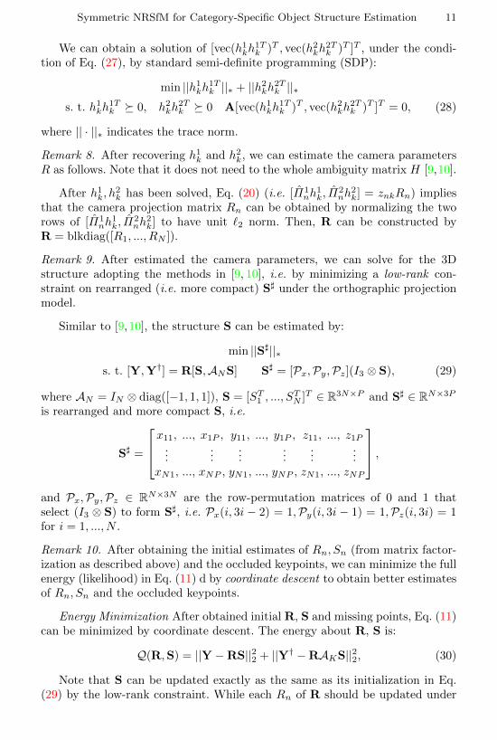
Symmetric NRSfM for Category-Specific Object Structure Estimation 11
We can obtain a solution of [vec(h1kh1Tk )T , vec(h2kh
2Tk )T ]T , under the condi-
tion of Eq. (27), by standard semi-definite programming (SDP):
min ||h1kh1Tk ||∗ + ||h2kh2Tk ||∗s. t. h1kh
1Tk � 0, h2kh
2Tk � 0 A[vec(h1kh
1Tk )T , vec(h2kh
2Tk )T ]T = 0, (28)
where || · ||∗ indicates the trace norm.
Remark 8. After recovering h1k and h2k, we can estimate the camera parametersR as follows. Note that it does not need to the whole ambiguity matrix H [9,10].
After h1k, h2k has been solved, Eq. (20) (i.e. [Π1
nh1k, Π
2nh
2k] = znkRn) implies
that the camera projection matrix Rn can be obtained by normalizing the tworows of [Π1
nh1k, Π
2nh
2k] to have unit `2 norm. Then, R can be constructed by
R = blkdiag([R1, ..., RN ]).
Remark 9. After estimated the camera parameters, we can solve for the 3Dstructure adopting the methods in [9, 10], i.e. by minimizing a low-rank con-straint on rearranged (i.e. more compact) S] under the orthographic projectionmodel.
Similar to [9, 10], the structure S can be estimated by:
min ||S]||∗s. t. [Y,Y†] = R[S,ANS] S] = [Px,Py,Pz](I3 ⊗ S), (29)
where AN = IN ⊗ diag([−1, 1, 1]), S = [ST1 , ..., STN ]T ∈ R3N×P and S] ∈ RN×3P
is rearranged and more compact S, i.e.
S] =
x11, ..., x1P , y11, ..., y1P , z11, ..., z1P......
......
......
xN1, ..., xNP , yN1, ..., yNP , zN1, ..., zNP
,and Px,Py,Pz ∈ RN×3N are the row-permutation matrices of 0 and 1 thatselect (I3 ⊗ S) to form S], i.e. Px(i, 3i − 2) = 1,Py(i, 3i − 1) = 1,Pz(i, 3i) = 1for i = 1, ..., N .
Remark 10. After obtaining the initial estimates of Rn, Sn (from matrix factor-ization as described above) and the occluded keypoints, we can minimize the fullenergy (likelihood) in Eq. (11) d by coordinate descent to obtain better estimatesof Rn, Sn and the occluded keypoints.
Energy Minimization After obtained initial R, S and missing points, Eq. (11)can be minimized by coordinate descent. The energy about R, S is:
Q(R,S) = ||Y −RS||22 + ||Y† −RAKS||22, (30)
Note that S can be updated exactly as the same as its initialization in Eq.(29) by the low-rank constraint. While each Rn of R should be updated under
12 Y. Gao and A. Yuille
the nonlinear orthonormality constraints RnRTn = I similar to the idea in EM-
PPCA [5]: we first parameterize Rn to a full 3×3 rotation matrix Q and updateQ by its rotation increment. Please refer to Appendix A3.
The occluded points Yn,p and Y †n,p with (n, p) ∈ IV S are updated by mini-mizing the full energy in Eq. (11) directly:
Yn,p = RnSp, Y †n,p = RnASn,p (31)
Similar to Sym-RSfM [26], after updating the occluded points, we also re-estimate the translation for each image by tn =
∑p(Yn,p−RnSp+Y †n,p−RnASp),
then centralize the data again by Yn ← Yn − 1TP ⊗ tn and Y †n ← Y †n − 1TP ⊗ tn.
5 Experiments
5.1 Experimental Settings
We follow the experimental settings in [24], using the 2D annotations in [39] and3D keypoints in Pascal3D+ [27]. Although Pascal3D+ is the best 3D datasetavailable, it still has some limitations for our task. Specifically, it does not havethe complete 3D models for each object; instead it provides the 3D shapes ofobject subtypes. For example, it provides 10 subtypes for car category, such assedan, truck, which ignores the shape variance within each subtype.
Similar to [7, 9, 10, 35], the rotation error eR and shape error eS are usedfor evaluation. We normalize 3D groundtruth and our 3D estimates to eliminatedifferent scales they may have. For each shape Sn we use its standard deviationsin X,Y, Z coordinates σxn, σ
yn, σ
zn for the normalization: Snorm
n = 3Sn/(σxn+σyn+
σzn). To deal with the rotation ambiguity between the 3D groundtruth and ourreconstruction, we use the Procrustes method [40] to align them. Then, the therotation error eR and shape error eS can be calculated as:
eR =1
N
N∑n=1
||Ralignedn −R∗n||F , eS =
1
2NP
N∑n=1
2P∑p=1
||Snorm alignedn,p − Snorm∗
n,p ||F ,
(32)where Raligned
n and R∗n are the recovered and the groundtruth camera projectionmatrix for image n. Snorm aligned
n,p and Snorm∗n,p are the normalized estimated and
the normalized groundtruth structure for the p’th point of image n. Ralignedn and
R∗n, Snorm alignedn,p and Snorm∗
n,p are aligned by Procrustes method [40].
5.2 Experimental Results on the Annotated Dataset
In this section, we construct the 3D keypoints for each image using the non-rigid model. Firstly, we follow the experimental setting in [24] and collect allimages with more than 5 visible keypoints. Then, we do 10 iterations with rank3 recovery to initialize the occluded/missing data. In this experiments, we use 3deformation bases and set λ in Sym-EM-PPCA, i.e. in Eqs. (9), as 1.
Symmetric NRSfM for Category-Specific Object Structure Estimation 13
aeroplane bus
I II III IV V VI VII mRE I II III IV V VI mRE
EP 0.36 0.59 0.50 0.49 0.57 0.57 0.45 0.34 0.42 0.34 0.56 0.54 0.98 0.86 0.26PF 0.99 1.08 1.13 1.15 1.22 1.10 1.11 0.52 1.62 1.56 1.75 1.59 2.09 1.70 0.47Sym-EP 0.33 0.53 0.46 0.43 0.51 0.53 0.46 0.31 0.28 0.25 0.33 0.33 0.65 0.46 0.21Sym-PF 0.57 0.76 0.84 0.76 0.73 0.61 0.79 0.46 1.92 1.95 1.77 1.54 1.70 1.42 1.23
car sofa
I II III IV V VI VII VIII IX X mRE I II III
EP 1.10 1.01 1.09 1.05 1.03 1.07 0.99 1.46 1.00 0.85 0.39 2.00 1.87 2.03PF 1.76 1.67 1.76 1.77 1.65 1.79 1.67 1.57 1.70 1.42 0.86 1.71 1.41 1.46Sym-EP 0.99 0.89 1.05 1.02 0.92 1.00 0.89 1.39 0.95 0.68 0.34 1.18 0.81 1.08Sym-PF 1.74 1.41 1.70 1.48 1.69 1.58 1.43 1.69 1.52 1.30 0.79 1.33 1.15 1.36
sofa train tv
IV V VI mRE I II III IV mRE I II III IV mRE
EP 1.99 2.37 1.81 0.79 1.18 0.53 0.49 0.42 0.85 0.44 0.51 0.44 0.36 0.41PF 2.02 2.66 1.64 1.36 1.97 0.27 0.47 0.34 0.98 0.56 1.01 0.97 0.65 0.80Sym-EP 1.12 1.80 0.88 0.34 0.95 0.46 0.42 0.31 0.73 0.51 0.60 0.53 0.64 0.52Sym-PF 1.02 1.17 0.95 0.85 1.52 0.40 0.49 0.47 0.99 0.60 1.01 1.15 0.51 0.86
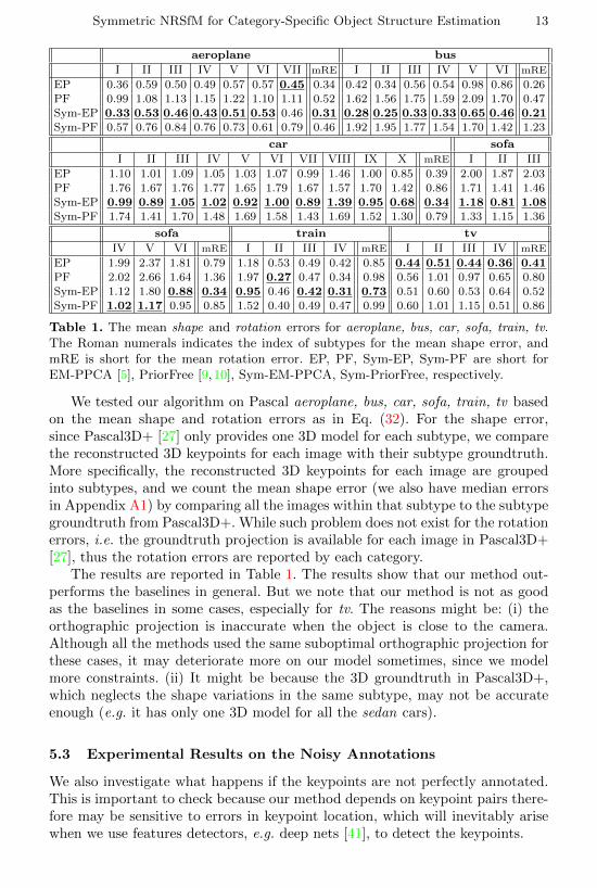
Table 1. The mean shape and rotation errors for aeroplane, bus, car, sofa, train, tv.The Roman numerals indicates the index of subtypes for the mean shape error, andmRE is short for the mean rotation error. EP, PF, Sym-EP, Sym-PF are short forEM-PPCA [5], PriorFree [9, 10], Sym-EM-PPCA, Sym-PriorFree, respectively.
We tested our algorithm on Pascal aeroplane, bus, car, sofa, train, tv basedon the mean shape and rotation errors as in Eq. (32). For the shape error,since Pascal3D+ [27] only provides one 3D model for each subtype, we comparethe reconstructed 3D keypoints for each image with their subtype groundtruth.More specifically, the reconstructed 3D keypoints for each image are groupedinto subtypes, and we count the mean shape error (we also have median errorsin Appendix A1) by comparing all the images within that subtype to the subtypegroundtruth from Pascal3D+. While such problem does not exist for the rotationerrors, i.e. the groundtruth projection is available for each image in Pascal3D+[27], thus the rotation errors are reported by each category.
The results are reported in Table 1. The results show that our method out-performs the baselines in general. But we note that our method is not as goodas the baselines in some cases, especially for tv. The reasons might be: (i) theorthographic projection is inaccurate when the object is close to the camera.Although all the methods used the same suboptimal orthographic projection forthese cases, it may deteriorate more on our model sometimes, since we modelmore constraints. (ii) It might be because the 3D groundtruth in Pascal3D+,which neglects the shape variations in the same subtype, may not be accurateenough (e.g. it has only one 3D model for all the sedan cars).
5.3 Experimental Results on the Noisy Annotations
We also investigate what happens if the keypoints are not perfectly annotated.This is important to check because our method depends on keypoint pairs there-fore may be sensitive to errors in keypoint location, which will inevitably arisewhen we use features detectors, e.g. deep nets [41], to detect the keypoints.

14 Y. Gao and A. Yuille
σ = 0.03 dmax σ = 0.05 dmax
I II III IV V VI VII mRE I II III IV
EP 0.34 0.59 0.49 0.45 0.54 0.55 0.45 0.33 0.37 0.58 0.51 0.47
PF 0.92 1.01 1.05 1.06 1.13 1.03 1.06 0.52 0.93 1.04 1.05 1.08
Sym-EP 0.34 0.54 0.47 0.44 0.52 0.55 0.46 0.32 0.35 0.54 0.47 0.43
Sym-PF 0.79 0.93 1.01 0.93 0.91 0.79 0.94 0.60 0.83 0.99 1.09 0.98
σ = 0.05 dmax σ = 0.07 dmax
V VI VII mRE I II III IV V VI VII mRE
EP 0.57 0.57 0.47 0.35 0.38 0.61 0.50 0.45 0.61 0.57 0.47 0.36
PF 1.15 1.02 1.07 0.54 0.94 1.04 1.08 1.07 1.15 1.03 1.08 0.65
Sym-EP 0.52 0.57 0.46 0.33 0.37 0.58 0.49 0.44 0.58 0.57 0.47 0.35
Sym-PF 0.94 0.84 1.04 0.63 0.94 1.06 1.15 1.04 1.05 0.89 1.08 0.70
Table 2. The mean shape and rotation errors for aeroplane with imperfect annotations.The noise is Gaussian N (0, σ2) with σ = sdmax, where we choose s = 0.03, 0.05, 0.07and dmax is the longest distance between all the keypoints (i.e. the tip of the nose tothe tip of the tail for aeroplane). Other parameters are the same as those in Table 1.Each result value is obtained by averaging 10 repetitions.
To simulate this, we add Gaussian noise N (0, σ2) to the 2D annotations andre-do the experiments. The standard deviation is set to σ = sdmax, where dmaxis the longest distance between all the keypoints (e.g. for aeroplane, it is thedistance between the nose tip to the tail tip). We have tested for different s by:0.03, 0.05, 0.07. The other parameters are the same as the previous section.
The results for aeroplane with s = 0.03, 0.05, 0.07 are shown in Table 2. Eachresult value is obtained by averaging 10 repetitions. The results in Table 2 showthat the performances of all the methods decrease in general with the increasein the noise level. Nonetheless, our methods still outperform our counterpartswith the noisy annotations (i.e. the imperfectly labeled annotations).
6 Conclusion
This paper shows that non-rigid SfM can be extended to the important specialcase where the objects are symmetric, which is frequently possessed by man-made objects [15, 16]. We derive and implement this extension to two popularnon-rigid structure from motion algorithms [5, 9, 10], which perform well on thePascal3D+ dataset when compared to the baseline methods.
In this paper, we have focused on constructing the non-rigid SfM model(s)that can exploit the symmetry property. In future work, we will extend to per-spective projection, apply a better initialization of the occluded keypoints suchas low-rank recovery, use additional object features (instead of just key-points),and detect these features from images automatically such as [41].
7 Acknowledgment
We would like to thank Ehsan Jahangiri, Cihang Xie, Weichao Qiu, Xuan Dong,Siyuan Qiao for giving feedbacks on the manuscript. This work was supportedby ARO 62250-CS and ONR N00014-15-1-2356.
Symmetric NRSfM for Category-Specific Object Structure Estimation 15
References
1. Tomasi, C., Kanade, T.: Shape and motion from image streams under orthography:a factorization method. International Journal of Computer Vision 9(2) (1992) 137–154
2. Hartley, R.I., Zisserman, A.: Multiple View Geometry in Computer Vision. Secondedn. Cambridge University Press (2004)
3. Torresani, L., Hertzmann, A., Bregler, C.: Learning non-rigid 3d shape from 2dmotion. In: NIPS. (2003)
4. Xiao, J., Chai, J., Kanade, T.: A closed-form solution to nonrigid shape and motionrecovery. In: ECCV. (2004)
5. Torresani, L., Hertzmann, A., Bregler, C.: Nonrigid structure-from-motion: Esti-mating shape and motion with hierarchical priors. IEEE Transactions on PatternAnalysis and Machine Intelligence 30 (2008) 878–892
6. Akhter, I., Sheikh, Y., Khan, S., Kanade, T.: Trajectory space: A dual representa-tion for nonrigid structure from motion. IEEE Transactions on Pattern Analysisand Machine Intelligence 33(7) (2011) 1442–1456
7. Gotardo, P., Martinez, A.: Computing smooth timetrajectories for camera anddeformable shape in structure from motion with occlusion. IEEE Transactions onPattern Analysis and Machine Intelligence 33 (2011) 2051–2065
8. Hamsici, O.C., Gotardo, P.F., Martinez, A.M.: Learning spatially-smooth map-pings in non-rigid structure from motion. In: ECCV. (2012) 260–273
9. Dai, Y., Li, H., He, M.: A simple prior-free method for non-rigid structure-from-motion factorization. In: CVPR. (2012)
10. Dai, Y., Li, H., He, M.: A simple prior-free method for non-rigid structure-from-motion factorization. International Journal of Computer Vision 107 (2014) 101–122
11. Ma, J., Zhao, J., Ma, Y., Tian, J.: Non-rigid visible and infrared face registrationvia regularized gaussian fields criterion. Pattern Recognition 48(3) (2015) 772–784
12. Ma, J., Zhao, J., Tian, J., Tu, Z., Yuille, A.L.: Robust estimation of nonrigidtransformation for point set registration. In: CVPR. (2013)
13. Ma, J., Zhao, J., Tian, J., Bai, X., Tu, Z.: Regularized vector field learning withsparse approximation for mismatch removal. Pattern Recognition 46(12) (2013)3519–3532
14. Agudo, A., Agapito, L., Calvo, B., Montiel, J.: Good vibrations: A modal analysisapproach for sequential non-rigid structure from motion. In: CVPR. (2014) 1558–1565
15. Rosen, J.: Symmetry discovered: Concepts and applications in nature and science.Dover Publications (2011)
16. Hong, W., Yang, A.Y., Huang, K., Ma, Y.: On symmetry and multiple-view geom-etry: Structure, pose, and calibration from a single image. International Journalof Computer Vision 60 (2004) 241–265
17. Gordon, G.G.: Shape from symmetry. In: Proc. SPIE. (1990)18. Kontsevich, L.L.: Pairwise comparison technique: a simple solution for depth re-
construction. JOSA A 10(6) (1993) 1129–113519. Vetter, T., Poggio, T.: Symmetric 3d objects are an easy case for 2d object recog-
nition. Spatial Vision 8 (1994) 443–45320. Mukherjee, D.P., Zisserman, A., Brady, M.: Shape from symmetry: Detecting
and exploiting symmetry in affine images. Philosophical Transactions: PhysicalSciences and Engineering 351 (1995) 77–106
16 Y. Gao and A. Yuille
21. Thrun, S., Wegbreit, B.: Shape from symmetry. In: ICCV. (2005)22. Li, Y., Pizlo, Z.: Reconstruction of shapes of 3d symmetric objects by using pla-
narity and compactness constraints. In: Proc. of SPIE-IS&T Electronic Imaging.(2007)
23. Vicente, S., Carreira, J., Agapito, L., Batista, J.: Reconstructing pascal voc. In:CVPR. (2014)
24. Kar, A., Tulsiani, S., Carreira, J., Malik, J.: Category-specific object reconstructionfrom a single image. In: CVPR. (2015)
25. Akhter, I., Sheikh, Y., Khan, S.: In defense of orthonormality constraints fornonrigid structure from motion. In: CVPR. (2009)
26. Gao, Y., Yuille, A.L.: Exploiting symmetry and/or Manhattan properties for3D object structure estimation from single and multiple images. arXiv preprintarXiv:1607.07129 (2016)
27. Xiang, Y., Mottaghi, R., Savarese, S.: Beyond pascal: A benchmark for 3d objectdetection in the wild. In: WACV. (2014)
28. Grossmann, E., Santos-Victor, J.: Maximum likehood 3d reconstruction from oneor more images under geometric constraints. In: BMVC. (2002)
29. Grossmann, E., Santos-Victor, J.: Least-squares 3d reconstruction from one ormore views and geometric clues. Computer Vision and Image Understanding 99(2)(2005) 151–174
30. Grossmann, E., Ortin, D., Santos-Victor, J.: Single and multi-view reconstructionof structured scenes. In: ACCV. (2002)
31. Kontsevich, L.L., Kontsevich, M.L., Shen, A.K.: Two algorithms for reconstructingshapes. Optoelectronics, Instrumentation and Data Processing 5 (1987) 76–81
32. Bregler, C., Hertzmann, A., Biermann, H.: Recovering non-rigid 3d shape fromimage streams. In: CVPR. (2000)
33. Hong, J.H., Fitzgibbon, A.: Secrets of matrix factorization: Approximations, nu-merics, manifold optimization and random restarts. In: ICCV. (2015)
34. Olsen, S.I., Bartoli, A.: Implicit non-rigid structure-from-motion with priors. Jour-nal of Mathematical Imaging and Vision 31(2-3) (2008) 233–244
35. Akhter, I., Sheikh, Y., Khan, S., Kanade, T.: Nonrigid structure from motion intrajectory space. In: NIPS. (2008)
36. Ceylan, D., Mitra, N.J., Zheng, Y., Pauly, M.: Coupled structure-from-motionand 3d symmetry detection for urban facades. ACM Transactions on Graphics 33(2014)
37. Morris, D.D., Kanatani, K., Kanade, T.: Gauge fixing for accurate 3d estimation.In: CVPR. (2001)
38. Bishop, C.M.: Pattern Recognition and Machine Learning. Springer, New York(2006)
39. Bourdev, L., Maji, S., Brox, T., Malik, J.: Detecting people using mutually con-sistent poselet activations. In: ECCV. (2010)
40. Schonemann, P.H.: A generalized solution of the orthogonal procrustes problem.Psychometrika 31 (1966) 1–10
41. Chen, X., Yuille, A.L.: Articulated pose estimation by a graphical model withimage dependent pairwise relations. In: NIPS. (2014) 1736–1744
Symmetric NRSfM for Category-Specific Object Structure Estimation 17
Appendix
This appendix contains more details of Symmetric Non-Rigid Structure fromMotion for Category-Specific Object Structure Estimation:
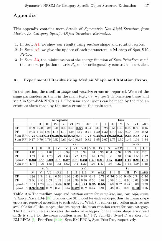
1. In Sect. A1, we show our results using median shape and rotation errors.
2. In Sect. A2, we give the update of each parameters in M-step of Sym-EM-PPCA.
3. In Sect. A3, the minimization of the energy function of Sym-PriorFree w.r.t.the camera projection matrix Rn under orthogonality constrains is detailed.
A1 Experimental Results using Median Shape and Rotation Errors
In this section, the median shape and rotation errors are reported. We used thesame parameters as them in the main text, i.e. we use 3 deformation bases andset λ in Sym-EM-PPCA as 1. The same conclusions can be made by the medianerrors as them made by the mean errors in the main text.
aeroplane bus
I II III IV V VI VII mRE I II III IV V VI mRE
EP 0.29 0.50 0.39 0.41 0.5 0.46 0.38 0.24 0.34 0.28 0.54 0.49 0.92 0.80 0.15PF 0.94 1.14 1.21 1.16 1.13 1.05 1.17 0.41 1.50 1.32 1.79 1.53 2.36 1.56 0.33Sym-EP 0.25 0.53 0.34 0.36 0.43 0.42 0.40 0.23 0.25 0.24 0.32 0.27 0.65 0.38 0.12Sym-PF 0.47 0.70 0.79 0.52 0.60 0.46 0.65 0.33 1.95 2.07 1.75 1.52 1.46 1.01 1.34
car sofa
I II III IV V VI VII VIII IX X mRE I II III
EP 1.05 1.01 1.07 1.01 0.99 1.07 0.94 1.44 0.95 0.84 0.37 1.99 1.86 2.01PF 1.71 1.66 1.73 1.79 1.60 1.72 1.75 1.48 1.70 1.36 0.81 1.76 1.55 1.32Sym-EP 0.93 0.88 1.02 0.99 0.87 0.99 0.83 1.40 0.91 0.67 0.32 1.12 0.81 1.07Sym-PF 1.73 1.26 1.81 1.43 1.62 1.54 1.32 1.70 1.47 1.16 0.67 1.14 1.08 1.18
sofa train tv
IV V VI mRE I II III IV mRE I II III IV mRE
EP 1.98 2.34 1.81 0.76 1.04 0.45 0.49 0.42 0.71 0.36 0.40 0.40 0.34 0.26PF 2.03 2.51 1.53 1.42 1.81 0.38 0.48 0.30 0.87 0.56 1.01 0.96 0.61 0.66Sym-EP 1.11 1.79 0.88 0.24 0.91 0.44 0.41 0.25 0.55 0.53 0.52 0.47 0.60 0.28Sym-PF 0.87 0.90 0.92 0.76 1.67 0.32 0.52 0.47 0.91 0.48 0.91 0.98 0.13 0.76
Table A3. The median shape and rotation errors for aeroplane, bus, car, sofa, train,tv. Since Pascal3D+ [27] provides one 3D model for each subtype, thus the mean shapeerrors are reported according to each subtype. While the camera projection matrices areavailable for all the images, thus we report the mean rotation errors for each category.The Roman numerals indicates the index of subtypes for the mean shape error, andmRE is short for the mean rotation error. EP, PF, Sym-EP, Sym-PF are short forEM-PPCA [5], PriorFree [9, 10], Sym-EM-PPCA, Sym-PriorFree, respectively.

18 Y. Gao and A. Yuille
A2 M-Step of Sym-EM-PPCA
This step is to maximize the complete (joint) log-likelihood P (Yn,Y†n,V|zn;Gn,S,V†,T). The complete log-likelihood Q(θ) is:
Q(θ) =−∑n
lnP (Yn,Y†n|zn;Gn, S,V,V†,T) + λ||V† −APV||2
=−∑n
(lnP (Yn|zn;Gn, S,V,T) + lnP (Y†n|zn;Gn, S,V†,T)
)+ λ||V† −APV||2
=2PN ln(2πσ2) +1
2σ2
∑n
Ezn ||Yn −Gn(S + Vzn)− Tn||2
+1
2σ2
∑n
Ezn ||Y†n −Gn(AP S + V†zn)− Tn||2 + λ||V −APV†||2
s. t. RnRTn = I, (33)
where θ = {Gn, S,V,V†,Tn, σ2}. Yn ∈ R2P×1, S ∈ R3P×1, and Tn ∈ R2P×1 arethe stacked vectors of 2D keypoints, 3D mean structure and translations. Gn =IP ⊗ cnRn, in which cn is the scale parameter for weak perspective projection,V = [V1, ...,VK ] ∈ R3P×K is the grouped K deformation bases, zn ∈ RK×1 isthe coefficient of the K bases. A = IP ⊗A, and A = diag([−1, 1, 1]) is a matrixoperator which negates the first row of its right matrix.
We first update the shape parameters S,V,V† by maximize the log-likelihoodQ. Since these 3 parameters are related to each other in their derivations, thusthey should be updated jointly by setting the 3 derivations to 0. According toEq. (33), we have: A∗, (B∗)T , C∗
B∗, D∗ + 2λσ2I3PK , −IK ⊗ 2λσ2APB∗AP , −IK ⊗ 2λσ2ATP , D∗ + IK ⊗ 2λσ2ATPAP
Svec(V)vec(V†)
=
vec(∑
nGTn (Y− Tn) +ATPGTn (Y† − Tn)
)vec(∑
nGTn (Y− Tn)µTn
)vec(∑
nGTn (Y† − Tn)µTn
),
, (34)
where we have:
A∗ =∑n
GTnGn +ATPGTnGnAP , B∗ =∑n
µn ⊗GTnGn
C∗ =∑n
µTn ⊗ATPGTnGn, D∗ =∑n
φTn ⊗GTnGn. (35)
The camera parameters tn, cn, Rn and the variance of the noise σ2 can beupdated similarly as Bregler’s method [5]. We first replace some parameters tomake the equation to be homogeneous:
V = [S,V], V† = [APS,V†],
µn = [1, µTn ]T , φn =
[1 µTnµn φn
](36)

Symmetric NRSfM for Category-Specific Object Structure Estimation 19
Then the estimations of new σ2, tn, cn are:
σ2 =1
4PN
∑n
(||Yn − Tn||2 + ||Y†n − Tn||2
−2(Yn − Tn)GnVµn − 2(Y†n − Tn)GnV†µn
+tr(VTGTnGnVφn) + tr(V†TGTnGnV†φn))
(37)
tn =1
2P
P∑p=1
(Yn,p − cnRnVpµn + Y†n,p − cnRnV†pµn) (38)
cn =
∑Pp=1
(µn
T VTp R
Tn (Yn,p − tn) + µn
T V†Tp RTn (Y†n,p − tn))
∑Pp=1 tr(VT
p RTnRnVpφn + V†Tp RTnRnV†pφn)
(39)
Since Rn is subject to a nonlinear orthonormality constraint and cannot beupdated in closed form, we follow an alternative approach used in [5] to param-eterize Rn as a complete 3 × 3 rotation matrix Qn and update the incrementalrotation on Qn instead, i.e. Qnewn = eξQn.
Here, the first and second rows of Qn is the same as Rn, and the third row ofQn is obtained by the cross product of its first and second rows. The relationshipof Qn and Rn can be revealed by a matrix operator M:
Rn =MQn, M =
[1, 0, 00, 1, 0
]. (40)
Note that the incremental rotation eξ can be further approximated by itsfirst order Taylor Series, i.e. eξ ≈ I + ξ. Finally, we have:
Rnewn (ξ) =M(I + ξ)Qn. (41)
Therefore, setting ∂Q/∂Rn = 0, then replace Rn by Qn using Eq. (41) andvectorize it, we have:
Rn =MeξQn ≈M(I + ξ)Qn and vec(ξ) = α+β (42)
α =
(c2n
P∑p=1
(VTp φnVp + V†Tp φnV†p)
TQTn
)⊗M; (43)
β =vec
(cn
P∑p=1
((Yn,p − tn)µn
T VTp + (Y†n,p − tn)µn
T V†Tp
)
− c2nMQn
P∑p=1
(VTp φnVp + V†Tp φnV†p)
)(44)
where the subscript p means the pth keypoint, α+ means the pseudo inversematrix of α, ⊗ denotes Kronecker product.
20 Y. Gao and A. Yuille
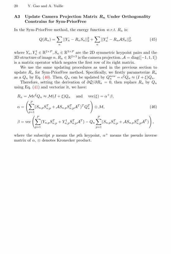
A3 Update Camera Projection Matrix Rn Under OrthogonalityConstrains for Sym-PriorFree
In the Sym-PriorFree method, the energy function w.r.t. Rn is:
Q(Rn) =∑n
||Yn −RnSn||22 +∑n
||Y †n −RnASn||22, (45)
where Yn, Y†n ∈ R2×P , Sn ∈ R3×P are the 2D symmetric keypoint pairs and the
3D structure of image n.Rn ∈ R2×3 is the camera projection.A = diag([−1, 1, 1])is a matrix operator which negates the first row of its right matrix.
We use the same updating procedures as used in the previous section toupdate Rn for Sym-PriorFree method. Specifically, we firstly parameterize Rnas a Qn by Eq. (40). Then, Qn can be updated by Qnewn = eξQn ≈ (I + ξ)Qn.
Therefore, setting the derivation of ∂Q/∂Rn = 0, then replace Rn by Qnusing Eq. (41) and vectorize it, we have:
Rn =MeξQn ≈M(I + ξ)Qn and vec(ξ) = α+β,
α =
(P∑p=1
(Sn,pSTn,p +ASn,pSTn,pAT )TQTn
)⊗M, (46)
β = vec
(P∑p=1
(Yn,pSTn,p + Y †n,pS
Tn,pAT )−Qn
P∑p=1
(Sn,pSTn,p +ASn,pSTn,pAT )
),
where the subscript p means the pth keypoint, α+ means the pseudo inversematrix of α, ⊗ denotes Kronecker product.