Symmetric Cross Entropy for Robust Learning with Noisy Labels

Yisen Wang1∗† Xingjun Ma2∗† Zaiyi Chen3 Yuan Luo1 Jinfeng Yi4 James Bailey2

1Shanghai Jiao Tong University 2The University of Melbourne 3Cainiao AI 4JD AI

Abstract

Training accurate deep neural networks (DNNs) in the

presence of noisy labels is an important and challenging

task. Though a number of approaches have been proposed

for learning with noisy labels, many open issues remain. In

this paper, we show that DNN learning with Cross Entropy

(CE) exhibits overfitting to noisy labels on some classes

(“easy” classes), but more surprisingly, it also suffers from

significant under learning on some other classes (“hard”

classes). Intuitively, CE requires an extra term to facilitate

learning of hard classes, and more importantly, this term

should be noise tolerant, so as to avoid overfitting to noisy

labels. Inspired by the symmetric KL-divergence, we pro-

pose the approach of Symmetric cross entropy Learning

(SL), boosting CE symmetrically with a noise robust coun-

terpart Reverse Cross Entropy (RCE). Our proposed SL ap-

proach simultaneously addresses both the under learning

and overfitting problem of CE in the presence of noisy la-

bels. We provide a theoretical analysis of SL and also em-

pirically show, on a range of benchmark and real-world

datasets, that SL outperforms state-of-the-art methods. We

also show that SL can be easily incorporated into existing

methods in order to further enhance their performance.

1. Introduction

Modern deep neural networks (DNNs) are often highly

complex models that have hundreds of layers and millions

of trainable parameters, requiring large-scale datasets with

clean label annotations such as ImageNet [2] for proper

training. However, labeling large-scale datasets is a costly

and error-prone process, and even high-quality datasets are

likely to contain noisy (incorrect) labels. Therefore, training

accurate DNNs in the presence of noisy labels has become

a task of great practical importance in deep learning.

Recently, several works have studied the dynamics of

DNN learning with noisy labels. Zhang et.al [28] argued

that DNNs exhibit memorization effects whereby they first

memorize the training data for clean labels and then subse-

quently memorize data for the noisy labels. Similar findings

∗Equal contribution. Part of work was done at JD AI Research.†Correspondence to: Yisen Wang (eewangyisen@gmail.com) and

Xingjun Ma (xingjun.ma@unimelb.edu.au).

(a) CE - clean (b) CE - noisy

(c) LSR - noisy (d) SL - noisy

Figure 1: The class-wise test accuracy of an 8-layer CNN

on CIFAR-10 trained by (a) CE on clean labels with class-

biased phenomenon, (b) CE on 40% symmetric/uniform

noisy labels with amplified class-biased phenomenon and

under learning on hard classes (e.g., class 3), (c) LSR under

the same setting to (b) with under learning on hard classes

still existing, (d) our proposed SL under the same setting to

(b) exhibiting overall improved learning on all classes.

are also reported in [1] that DNNs first learn clean and easy

patterns and eventually memorize the wrongly assigned la-

bels. Further evidence is provided in [13] that DNNs first

learn simple representations via subspace dimensionality

compression and then overfit to noisy labels via subspace

dimensionality expansion. Different findings are reported

in [19], where DNNs with a specific activation function

(i.e., tanh) undergo an initial label fitting phase then a sub-

sequent representation compression phase where the over-

fitting starts. Despite these important findings, a complete

understanding of DNN learning behavior, particularly their

learning process for noisy labels, remains an open question.

In this paper, we provide further insights into the learn-

ing procedure of DNNs by investigating the learning dy-

namics across classes. While Cross Entropy (CE) loss is

the most commonly used loss for training DNNs, we have

found that DNN learning with CE can be class-biased:

322

(a) CE - clean (b) CE - noisy (c) SL - noisy

Figure 2: Visualization of learned representations on

CIFAR-10 using t-SNE 2D embeddings of deep features at

the last second dense layer with (a) CE on clean labels, (b)

CE on 40% symmetric noisy labels, (c) the proposed SL on

the same setting to (b).

some classes (“easy” classes) are easy to learn and con-

verge faster than other classes (“hard” classes). As shown

in Figure 1a, even when labels are clean, the class-wise test

accuracy spans a wide range during the entire training pro-

cess. As further shown in Figure 1b, this phenomenon is

amplified when training labels are noisy: whilst easy classes

(e.g., class 6) already overfit to noisy labels, hard classes

(e.g., class 3) still suffer from significant under learning

(class accuracy significantly lower than clean label setting).

Specifically, class 3 (bottom curve) only has an accuracy

of ∼60% at the end, considerably less than the >90% ac-

curacy of class 6 (top curve). Label Smoothing Regular-

ization (LSR) [21, 17] is a widely known technique to ease

overfitting issues, as shown in Figure 1c, which still exhibits

significant under learning on hard classes. Comparing the

overall test accuracy (solid red curve) in Figure 1, a low test

accuracy (under learning) on hard classes is a barrier to high

overall accuracy. This is a different finding from previous

belief that poor performance is simply caused by overfitting

to noisy labels. We also visualize the learned representa-

tions for the noisy label case in Figure 2b: some clusters

are learned comparably well to those learned with clean la-

bels (Figure 2a), while some other clusters do not have clear

separated boundaries.

Intuitively, CE requires an extra term to improve its

learning on hard classes, and more importantly, this term

needs to be tolerant to label noise. Inspired by the sym-

metric KL-divergence, we propose such a noise tolerant

term, namely Reverse Cross Entropy (RCE), which com-

bined with CE forms the basis of the approach Symmetric

cross entropy Learning (SL). SL not only promotes suffi-

cient learning (class accuracy close to clean label setting)

of hard classes, but also improves the robustness of DNNs

to noisy labels. As a preview of this, we can inspect the

improved learning curves of class-wise test accuracy and

representations in Figure 1d and 2c. Under the same 40%

noise setting, the variation of class-wise test accuracy has

been narrowed by SL to 20% with 95% the highest and 75%

the lowest (Figure 1d), and the learned representations are

of better quality with more separated clusters (Figure 2c),

both of which are very close to the clean settings.

Compared to existing approaches that often involve ar-

chitectural or non-trivial algorithmic modifications, SL is

extremely simple to use. It requires minimal intervention

to the training process and thus can be straightforwardly

incorporated into existing models to further enhance their

performance. In summary, our main contributions are:

• We provide insights into the class-biased learning pro-

cedure of DNNs with CE loss and find that the under

learning problem of hard classes is a key bottleneck for

learning with noisy labels.

• We propose a Symmetric Learning (SL) approach, to

simultaneously address the hard class under learning

problem and the noisy label overfitting problem of CE.

We provide both theoretical analysis and empirical un-

derstanding of SL.

• We empirically demonstrate that SL can achieve better

robustness than state-of-the-art methods, and can be

also easily incorporated into existing methods to sig-

nificantly improve their performance.

2. Related Work

Different approaches have been proposed to train accu-

rate DNNs with noisy labels, and they can be roughly di-

vided into three categories: 1) label correction methods, 2)

loss correction methods, and 3) refined training strategies.

The idea of label correction is to improve the quality of

the raw labels. One common approach is to correct noisy

labels to their true labels via a clean label inference step us-

ing complex noise models characterized by directed graphi-

cal models [26], conditional random fields [23], neural net-

works [11, 24] or knowledge graphs [12]. These methods

require the support from extra clean data or an expensive

detection process to estimate the noise model.

Loss correction methods modify the loss function for

robustness to noisy labels. One approach is to model the

noise transition matrix that defines the probability of one

class changed to another class [5]. Backward [16] and For-

ward [16] are two such correction methods that use the noise

transition matrix to modify the loss function. However, the

ground-truth noise transition matrix is not always available

in practice, and it is also difficult to obtain accurate estima-

tion [5]. Work in [4, 20] augments the correction architec-

ture by adding a linear layer on top of the neural network.

Bootstrap [18] uses a combination of raw labels and their

predicted labels. There is also research that defines noise

robust loss functions, such as Mean Absolute Error (MAE)

[3], but a challenge is that training a network with MAE is

slow due to gradient saturation. Generalized Cross Entropy

(GCE) loss [29] applies a Box-Cox transformation to prob-

abilities (power law function of probability with exponent

q) and can behave like a weighted MAE. Label Smoothing

Regularization (LSR) [21, 17] is another technique using

soft labels in place of one-hot labels to alleviate overfitting

to noisy labels.

323

Refined training strategies design new learning

paradigms for noisy labels. MentorNet [8, 27] super-

vises the training of a StudentNet by a learned sample

weighting scheme in favor of probably correct labels.

Decoupling training strategy [15] trains two networks

simultaneously, and parameters are updated when their

predictions disagree. Co-teaching [6] maintains two

networks simultaneously during training, with one network

learning from the other network’s most confident samples.

These studies all require training of an auxiliary network

for sample weighting or learning supervision. D2L [13]

uses subspace dimensionality adapted labels for learning,

paired with a training process monitor. The iterative learn-

ing framework [25] iteratively detects and isolates noisy

samples during the learning process. The joint optimization

framework [22] updates DNN parameters and labels alter-

nately. These methods either rely on complex interventions

into the learning process, which may be challenging to

adapt and tune, or are sensitive to hyperparameters like the

number of training epochs and learning rate.

3. Weakness of Cross Entropy

We begin by analyzing the Cross Entropy (CE) and its

limitations for learning with noisy labels.

3.1. Preliminaries

Given a K-class dataset D = {(x, y)(i)}ni=1, with x ∈X ⊂ R

d denoting a sample in the d-dimensional input space

and y ∈ Y = {1, · · · ,K} its associated label. For each

sample x, a classifier f(x) computes its probability of each

label k ∈ {1, · · · ,K}: p(k|x) = ezk∑Kj=1

ezj

, where zj are the

logits. We denote the ground-truth distribution over labels

for sample x by q(k|x), and∑K

k=1 q(k|x) = 1. Consider

the case of a single ground-truth label y, then q(y|x) = 1and q(k|x) = 0 for all k 6= y. The cross entropy loss for

sample x is:

ℓce = −

K∑

k=1

q(k|x) log p(k|x). (1)

3.2. Weakness of CE under Noisy Labels

We now highlight some weaknesses of CE for DNN

learning with noisy labels, based on empirical evidence on

CIFAR-10 dataset [9] (10 classes of natural images). To

generate noisy labels, we randomly flip a correct label to

one of the other 9 incorrect labels uniformly (e.g., symmet-

ric label noise), and refer to the portion of incorrect labels as

the noise rate. The network used here is an 8-layer convo-

lutional neural network (CNN). Detailed experimental set-

tings can be found in Section 5.1.

We first explore in more detail the class-biased phe-

nomenon shown in Figure 1a and 1b, focusing on three dis-

tinct learning stages: early (the 10-th epoch), middle (the

(a) CE - clean (b) CE - noisy

Figure 3: The class-wise test accuracy at epoch 10, 50 and

100 (120 epochs in total) trained by CE loss on CIFAR-10

with (a) clean labels or (b) 40% symmetric noisy labels.

(a) Prediction confidence (b) Prediction distribution

Figure 4: Intermediate results of CE loss on CIFAR-10 with

40% symmetric noisy labels. (a) Average confidence of the

clean portion of class 3 samples. (b) The true positive sam-

ples (correct) out of predictions (predicted) for each class.

50-th epoch) and later (the 100-th epoch) stages, with re-

spect to total 120 epochs of training. As illustrated in Fig-

ure 3, CE learning starts in a highly class-biased manner

(the blue curves) for both clean labels and 40% noisy labels.

This is because patterns inside of samples are intrinsically

different. For clean labels, the network eventually manages

to learn all classes uniformly well, reflected by the relatively

flat accuracy curve across classes (the green curve in Figure

3a). However, for noisy labels, the class-wise test accuracy

varies significantly across different classes, even at the later

stage (the green curve in Figure 3b). In particular, the net-

work struggles to learn hard classes (e.g., class 2/3) with

up to a 20% gap to the clean setting, whereas some easy

classes (e.g., class 1/6) are better learned and already start

overfitting to noisy labels (accuracy drops from epoch 50 to

100). It appears that the under learning of hard classes is

a major cause for the overall performance degradation, due

to the fact that the accuracy drop caused by overfitting is

relatively small.

We further investigate the reason behind the under learn-

ing of CE on hard classes from the perspective of represen-

tations. Due to their high similarities in representations to

some other classes (see the red cluster for class 3 in Figure

2a), the predictions for hard class examples are likely to as-

sign a relatively large probability to those similar classes.

Under the noisy label scenario, class 3 has become even

more scattered into other classes (red cluster in Figure 2b).

As a consequence, no visible cluster was learned by CE,

324

even though there are still 60% correct labels in this sce-

nario. Further delving into these 60% clean portion of class

3 samples, we show, in Figure 4a, their prediction confi-

dence output of the neural network. Although the confi-

dence at class 3 is the highest, it is only around 0.5, while

for the other classes, the confidence is around 0.05 or 0.1

which is actually a relatively high value and an indication

of insufficient learning of class 3 even on the clean labeled

part. Another evidence of under learning can be obtained

from Figure 4b, where hard classes (e.g., class 2/3) have

fewer true positive samples throughout intermediate stages

of learning.

Clearly, CE by itself is not sufficient for learning of hard

classes, especially under the noisy label scenario. We note

that this finding sheds new insights into DNN learning be-

havior under label noise, and differs from previous belief

that DNNs overfit to all classes in general [1, 28]. In the

next section, we propose a symmetric learning approach

that can address both the hard class under learning and noisy

label overfitting problems of CE.

4. Symmetric Cross Entropy Learning

In this section, we propose Symmetric cross entropy

Learning (SL), an approach that strikes a balance between

sufficient learning and robustness to noisy labels. We also

provide theoretical analysis about the formulation and be-

havior of SL.

4.1. Definition

Given two distributions q and p, the relation between the

cross entropy (denoted as H(q, p)) and the KL-divergence

(denoted as KL(q‖p)) is:

KL(q‖p) = H(q, p)−H(q), (2)

where H(q) is the entropy of q. In the context of classifica-

tion, q = q(k|x) is the ground truth class distribution condi-

tioned on sample x, whilst p = p(k|x) is the predicted dis-

tribution over labels by the classifier f . From the perspec-

tive of KL-divergence, classification is to learn a predic-

tion distribution p(k|x) that is close to the ground truth dis-

tribution q(k|x), which is to minimize the KL-divergence

KL(q‖p) between the two distributions∗.

In information theory, given a true distribution q and its

approximation p, KL(q‖p) measures the penalty on encod-

ing samples from q using code optimized for p (penalty in

the number of extra bits required). In the context of noisy

labels, we know that q(k|x) does not represent the true class

distribution, instead p(k|x) can reflect the true distribution

to a certain extent. Thus, in addition to taking q(k|x) as the

ground truth, we also need to consider the other direction of

KL-divergence, that is KL(p||q), to punish coding samples

∗In practice, the H(q(k|x)) term is a constant for a given class distri-

bution and therefore omitted from Eq. (2) giving the CE loss in Eq. (1).

that come from p(k|x) when using a code for q(k|x). The

symmetric KL-divergence is:

SKL = KL(q||p) +KL(p||q). (3)

Transferring this symmetric idea from KL-divergence to

cross entropy gives us the Symmetric Cross Entropy (SCE):

SCE = CE +RCE = H(q, p) +H(p, q), (4)

where RCE = H(p, q) is the reverse version of H(q, p),namely, Reverse Cross Entropy. The RCE loss for a sample

x is:

ℓrce = −

K∑

k=1

p(k|x) log q(k|x). (5)

The sample-wise SCE loss can then be defined as:

ℓsce = ℓce + ℓrce. (6)

While the RCE term is noise tolerant as will be proved

in Section 4.2, the CE term is not robust to label noise [3].

However, CE is useful for achieving good convergence [29],

which will be verified empirically in Section 5. Towards

more effective and robust learning, we propose a flexible

symmetric learning framework with the use of two decou-

pled hyperparameters (e.g., α and β), with α on the over-

fitting issue of CE while β for flexible exploration on the

robustness of RCE. Formally, the SL loss is:

ℓsl = αℓce + βℓrce. (7)

As the ground truth distribution q(k|x) is now inside of

the logarithm in ℓrce, this could cause computational prob-

lem when labels are one-hot: zero values inside the log-

arithm. To solve this issue, we define log 0 = A (where

A < 0 is some constant), which shortly will be proved

useful for the robustness of ℓrce in Theorem 1. This tech-

nique is similar to the clipping operation implemented by

most deep learning frameworks. Compared with another

option label smoothing technique, our approach introduces

less bias into the model (negligible bias (in the view of train-

ing) at finite number of points like q(k|x) = 0 but no bias

at q(k|x) = 1). Note that, the effect of β on RCE can be

reflected by different settings of A (refer to Eq. (4.3)).

4.2. Theoretical Analysis

Robustness analysis: In the following, we will prove that

the RCE loss ℓrce is robust to label noise following [3]. We

denote the noisy label of x as y, in contrast to its true label

y. Given any classifier f and loss function ℓrce, we define

the risk of f under clean labels as R(f) = Ex,yℓrce, and

the risk under label noise rate η as Rη(f) = Ex,yℓrce. Let

f∗ and f∗η be the global minimizers of R(f) and Rη(f) re-

spectively. Risk minimization under a given loss function

is noise robust if f∗η has the same probability of misclassi-

fication as that of f∗ on noise free data. When the above is

satisfied we also say that the loss function is noise-tolerant.

325

Theorem 1. In a multi-class classification problem, ℓrceis noise tolerant under symmetric or uniform label noise if

noise rate η < 1− 1K

. And, if R(f∗) = 0, ℓrce is also noise

tolerant under asymmetric or class-dependent label noise

when noise rate ηyk < 1− ηy with∑

k 6=y ηyk = ηy .

Proof. For symmetric noise:

Rη(f) = Ex,yℓrce = ExEy|xEy|x,yℓrce

= ExEy|x

[

(1− η)ℓrce +η

K − 1

K∑

k 6=y

ℓrce

]

= (1− η)R(f) +η

K − 1(

K∑

k=1

ℓrce −R(f))

= R(f)

(

1−ηK

K − 1

)

−Aη,

where the last equality holds due to∑K

k=1 ℓrce = −(K −1)A following Eq. (5) and definition of log 0 = A. Thus,

Rη(f∗)−Rη(f) = (1−ηK

K − 1)(R(f∗)−R(f)) ≤ 0

because η < 1 − 1K

and f∗ is a global minimizer of R(f).This proves f∗ is also the global minimizer of risk Rη(f),that is, ℓrce is noise tolerate.

Similarly, we can prove the case for asymmetric noise,

please refer Appendix A for details. �

Gradient analysis: We next derive the gradients of a sim-

plified SL with α, β = 1 to give a rough idea of how its

learning process differs from that of CE†. For brevity, we

denote pk, qk as abbreviations for p(k|x) and q(k|x). Con-

sider the case of a single true label, the gradient of the

sample-wise RCE loss with respect to the logits zj can be

derived as:

∂ℓrce∂zj

= −

K∑

k=1

∂pk∂zj

log qk, (8)

where ∂pk

∂zjcan be further derived based on whether k = j:

∂pk∂zj

=

{

pk(1− pk), k = j

−pjpk, k 6= j.(9)

According to Eq. (9) and the ground-truth distribution for

the case of one single label (e.g., qy = 1, and qk = 0 for

k 6= y), the gradients of SL can be derived as:

∂ℓsl∂zj

=

{

∂ℓce∂zj

− (Ap2j −Apj), qj = qy = 1∂ℓce∂zj

+ (−Apjpy), qj = 0,(10)

†Complete derivations can be found in the Appendix B.

where A is the smoothed/clipped replacement of log 0. Note

that the gradient of sample-wise CE loss ℓce is:

∂ℓce∂zj

=

{

pj − 1 ≤ 0, qj = qy = 1

pj ≥ 0, qj = 0.(11)

In the case of qj = qy = 1 (∂ℓce∂zj

≤ 0), the second

term Ap2j − Apj is an adaptive acceleration term based on

pj . Specifically, Ap2j − Apj is a convex parabolic function

in the first quadrant for pj ∈ [0, 1], and has the maximum

value at pj = 0.5. Considering the learning progresses to-

wards pj → 1, RCE increases DNN prediction on label ywith larger acceleration for pj < 0.5 and smaller acceler-

ation for pj > 0.5. In the case of qj = 0 (∂ℓce∂zj

≥ 0), the

second term −Apjpy is an adaptive acceleration on the min-

imization of the probability at unlabeled class (pj), based on

the confidence at the labeled class (py). Larger py leads to

larger acceleration, that is, if the network is more confident

about its prediction at the labeled class, then the residual

probabilities at other unlabeled classes should be reduced

faster. When py = 0, there is no acceleration, which means

if the network is not confident on the labeled class at all,

then the label is probably wrong, no acceleration needed.

4.3. Discussion

An easy addition to improve CE would be to upscale

its gradients with a larger coefficient (e.g., ‘2CE’, ‘5CE’).

However, this will cause more overfitting (see the ‘5CE’

curve in the following Section 5 Figure 9a). There are also

other options to consider, such as MAE. Although moti-

vated from completely different perspectives, that is, CE

and RCE are measures of (information theoretic) uncer-

tainty, while MAE is a measure of distance, we can surpris-

ingly show that MAE is a special case of RCE at A = −2,

when there is a single true label for x (e.g. q(y|x) = 1 and

q(k 6= y|x) = 0). For MAE, we have,

ℓmae =K∑

k=1

|p(k|x)− q(k|x)| = (1− p(y|x)) +∑

k 6=y

p(k|x)

= 2(1− p(y|x)),

while, for RCE, we have,

ℓrce = −

K∑

k=1

p(k|x) log q(k|x)

= −p(y|x) log 1−∑

k 6=y

p(k|x)A = −A∑

k 6=y

p(k|x)

= −A(1− p(y|x)).

That is, when A = −2, RCE is reduced to exactly MAE.

Meanwhile, different from the GCE loss (i.e., a weighted

MAE) [29], SL is a combination of two symmetrical learn-

ing terms.

326

5. Experiments

We first provide some empirical understanding of our

proposed SL approach, then evaluate its robustness against

noisy labels on MNIST, CIFAR-10, CIFAR-100, and a

large-scale real-world noisy dataset Clothing1M.

Noise setting: We test two types of label noise: symmetric

(uniform) noise and asymmetric (class-dependent) noise.

Symmetric noisy labels are generated by flipping the la-

bels of a given proportion of training samples to one of

the other class labels uniformly. Whilst for asymmetric

noisy labels, flipping labels only occurs within a specific

set of classes [16, 29], for example, for MNIST, flipping

2 → 7, 3 → 8, 5 ↔ 6 and 7 → 1; for CIFAR-10, flip-

ping TRUCK → AUTOMOBILE, BIRD → AIRPLANE,

DEER → HORSE, CAT ↔ DOG; for CIFAR-100, the 100

classes are grouped into 20 super-classes with each has 5

sub-classes, then flipping between two randomly selected

sub-classes within each super-class.

5.1. Empirical Understanding of SL

We conduct experiments on CIFAR-10 dataset with sym-

metric noise towards a deeper understanding of SL.

Experimental setup: We use an 8-layer CNN with 6

convolutional layers followed by 2 fully connected layers.

All networks are trained using SGD with momentum 0.9,

weight decay 10−4 and an initial learning rate of 0.01 which

is divided by 10 after 40 and 80 epochs (120 epochs in to-

tal). The parameter α, β and A in SL are set to 0.1, 1 and -6

respectively.

Class-wise learning: The class-wise test accuracy of SL on

40% noisy labels has already been presented in Figure 1d.

Here we provide further results for 60% noisy labels in Fig-

ure 5. Under both settings, each class is more sufficiently

learned by SL than CE, accompanied by accuracy increases.

Particularly for the hard classes (e.g., classes 2/3/4/5), SL

significantly improves their learning performance. This is

because SL facilitates an adaptive pace to encourage learn-

ing from hard classes. During learning, samples from easy

classes can be quickly learned to have a high probability

pk > 0.5, while samples from hard classes still have a low

probability pk < 0.5. SL will balance this discrepancy by

increasing the learning speed for samples with pk < 0.5while decreasing the learning speed for those with pk > 0.5.

Prediction confidence and distribution: In comparison to

the low confidence of CE on the clean samples in Figure

4a, we train the same network using SL under the same set-

ting. As shown in Figure 6a, on the clean portion of class

3 samples, SL successfully pulls up the confidence to 0.95,

while at the same time, pushes down the residual confidence

at other classes to almost 0. As further shown in Figure 6b,

the prediction distributions demonstrate that each class con-

tains more than 4000 true positive samples, including the

hard classes (e.g., class 2/3/4/5). Some classes (e.g., class

1/6/7/8/9) even obtain close to 5000 true positive samples

(the ideal case). Compared to the earlier results in Figure

(a) CE (b) SL

Figure 5: Class-wise test accuracy of CE and SL on CIFAR-

10 dataset with 60% symmetric noisy labels. The red solid

lines are the overall test accuracies.

(a) Prediction confidence (b) Prediction distribution

Figure 6: Effect of the proposed SL on prediction confi-

dence/distribution on CIFAR-10 with 40% noisy labels. (a)

Average confidence of the clean portion of class 3 samples.

(b) The true positive samples (correct) out of predictions

(predicted) for each class.

(a) CE (b) SL

Figure 7: Representations learned by CE and SL on CIFAR-

10 dataset with 60% symmetric noisy labels.

4b, SL achieves considerable improvement on each class.

Representations: We further investigate the representa-

tions learned by SL compared to that learned by CE. We

extract the high-dimensional representation at the second

last dense layer, then project to a 2D embedding using t-

SNE [14]. The projected representations are illustrated in

Figures 2 and 7 for 40% and 60% noisy labels respectively.

Under both settings, the representations learned by SL are

of significantly better quality than that of CE with more sep-

arated and clearly bounded clusters.

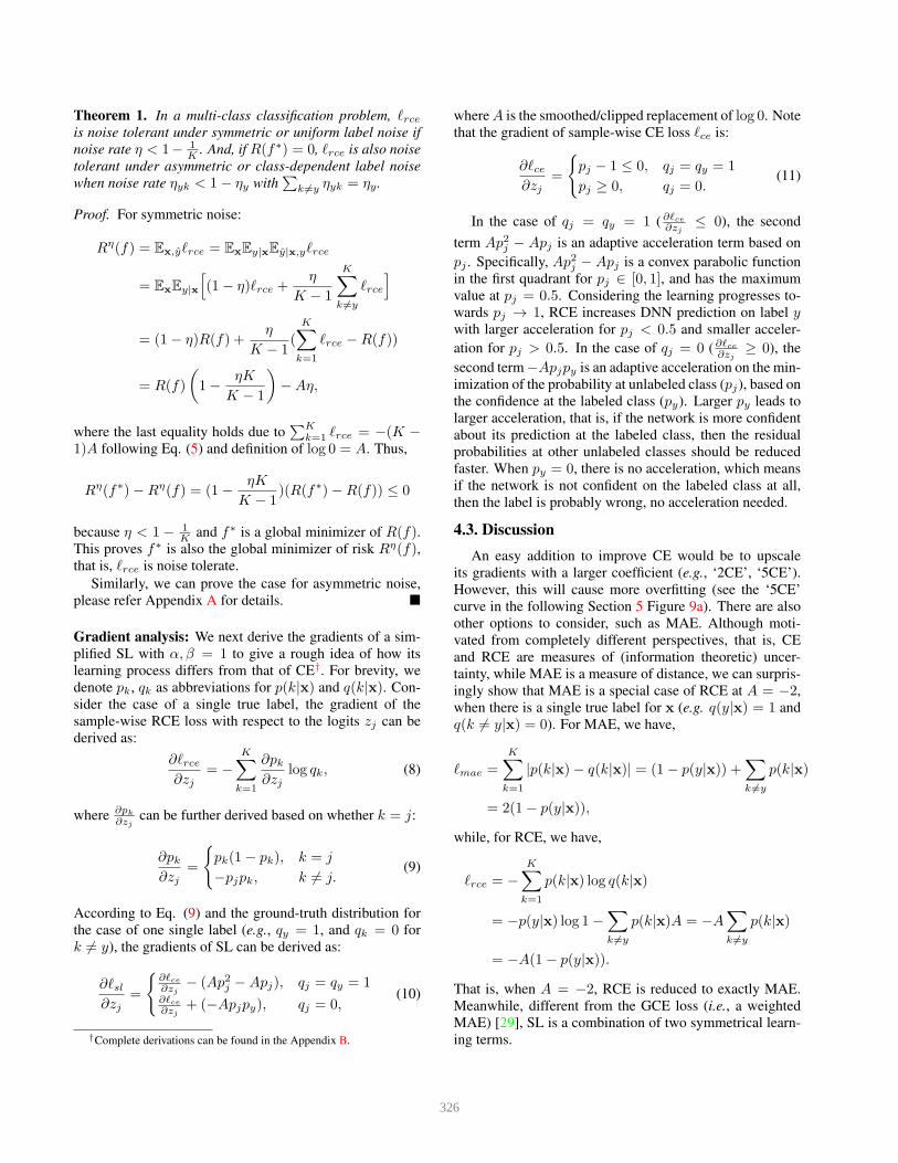
Parameter analysis: We tune the parameters of SL: α, βand A. As β can be reflected by A, here we only show

results of α and A. We tested A in [−8,−2] with step 2

and α ∈ [10−2, 1] on CIFAR-10 under 60% noisy labels.

Figure 8a shows that large α (e.g., 1.0/0.5) tends to cause

more overfitting, while small α (e.g., 0.1/0.01) can help ease

327

(a) α (A=-6) (b) A/β (α=0.1) (c) A/β (α=1)

Figure 8: Parameter analysis for SL with an 8-layer CNN

on CIFAR-10 dataset under 60% symmetric label noise: (a)

Tuning α (fix A = -6); (b) Tuning A/β (fix α = 0.1); and (c)

Tuning A/β (fix α = 1).

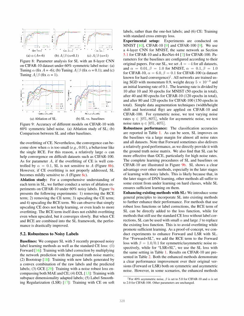
(a) Ablation of SL (b) SL vs. baselines

Figure 9: Accuracy of different models on CIFAR-10 with

60% symmetric label noise. (a) Ablation study of SL; (b)

Comparison between SL and other baselines.

the overfitting of CE. Nevertheless, the convergence can be-

come slow when α is too small (e.g., 0.01), a behaviour like

the single RCE. For this reason, a relatively large α can

help convergence on difficult datasets such as CIFAR-100.

As for parameter A, if the overfitting of CE is well con-

trolled by α = 0.1, SL is not sensitive to A (Figure 8b).

However, if CE overfitting is not properly addressed, SL

becomes mildly sensitive to A (Figure 8c).

Ablation study: For a comprehensive understanding of

each term in SL, we further conduct a series of ablation ex-

periments on CIFAR-10 under 60% noisy labels. Figure 9a

presents the following experiments: 1) removing the RCE

term; 2) removing the CE term; 3) upscaling the CE term;

and 4) upscaling the RCE term. We can observe that simply

upscaling CE does not help learning, or even leads to more

overfitting. The RCE term itself does not exhibit overfitting

even when upscaled, but it converges slowly. But when CE

and RCE are combined into the SL framework, the perfor-

mance is drastically improved.

5.2. Robustness to Noisy Labels

Baselines: We compare SL with 5 recently proposed noisy

label learning methods as well as the standard CE loss: (1)

Forward [16]: Training with label correction by multiplying

the network prediction with the ground truth noise matrix;

(2) Bootstrap [18]: Training with new labels generated by

a convex combination of the raw labels and the predicted

labels; (3) GCE [29]: Training with a noise robust loss en-

compassing both MAE and CE; (4) D2L [13]: Training with

subspace dimensionality adapted labels; (5) Label Smooth-

ing Regularization (LSR) [17]: Training with CE on soft

labels, rather than the one-hot labels; and (6) CE: Training

with standard cross entropy loss.

Experimental setup: Experiments are conducted on

MNIST [10], CIFAR-10 [9] and CIFAR-100 [9]. We use

a 4-layer CNN for MNIST, the same network as Section

5.1 for CIFAR-10 and a ResNet-44 [7] for CIFAR-100. Pa-

rameters for the baselines are configured according to their

original papers. For our SL, we set A = −4 for all datasets,

and α = 0.01, β = 1.0 for MNIST, α = 0.1, β = 1.0for CIFAR-10, α = 6.0, β = 0.1 for CIFAR-100 (a dataset

known for hard convergence)‡. All networks are trained us-

ing SGD with momentum 0.9, weight decay 5 × 10−3 and

an initial learning rate of 0.1. The learning rate is divided by

10 after 10 and 30 epochs for MNIST (50 epochs in total),

after 40 and 80 epochs for CIFAR-10 (120 epochs in total),

and after 80 and 120 epochs for CIFAR-100 (150 epochs in

total). Simple data augmentation techniques (width/height

shift and horizontal flip) are applied on CIFAR-10 and

CIFAR-100. For symmetric noise, we test varying noise

rates η ∈ [0%, 80%], while for asymmetric noise, we test

noise rates η ∈ [0%, 40%].Robustness performance: The classification accuracies

are reported in Table 1. As can be seen, SL improves on

the baselines via a large margin for almost all noise rates

and all datasets. Note that Forward sometimes also delivers

a relatively good performance, as we directly provide it with

the ground truth noise matrix. We also find that SL can be

more effective than GCE, particularly for high noise rates.

The complete learning procedures of SL and baselines on

CIFAR-10 are illustrated in Figure 9b. SL shows a clear

advantage over other methods, especially in the later stages

of learning with noisy labels. This is likely because that, in

the later stages of DNN learning, other methods all suffer to

some extent from under learning on hard classes, while SL

ensures sufficient learning on them.

Enhancing existing methods with SL: We introduce some

general principles to incorporate SL into existing methods

to further enhance their performance. For methods that use

robust loss functions or label corrections, the RCE term of

SL can be directly added to the loss function, while for

methods that still use the standard CE loss without label cor-

rections, SL can be used with small α and large β to replace

the existing loss function. This is to avoid overfitting while

promote sufficient learning. As a proof-of-concept, we con-

duct experiments to enhance Forward and LSR with SL.

For “Forward+SL”, we add the RCE term to the Forward

loss with β = 1.0/0.1 for symmetric/asymmetric noise re-

spectively, while for “LSR+SL”, we use the SL loss with

the same setting in Table 1. Results on CIFAR-10 are pre-

sented in Table 2. Both the enhanced methods demonstrate

a clear performance improvement over their original ver-

sions (Forward or LSR) both on symmetric and asymmetric

noise. However, in some scenarios, the enhanced methods

‡For 40% asymmetric noise, β is set to 5.0 for CIFAR-10 and α is set

to 2.0 for CIFAR-100. Other parameters are unchanged.

328

Table 1: Test accuracy (%) of different models on benchmark datasets with various rates of symmetric and asymmetric noisy

labels. The average accuracy and standard deviation of 5 random runs are reported and the best results are in bold.

Datasets Methods

Symmetric Noise Asymmetric Noise

Noise Rate η Noise Rate η0.0 0.2 0.4 0.6 0.8 0.2 0.3 0.4

MNIST

CE 99.02± 0.01 88.71± 0.05 69.56± 0.19 46.54± 0.28 21.77± 0.07 93.14± 0.04 87.91± 0.05 81.10± 0.07LSR 99.28± 0.01 89.56± 0.06 68.11± 0.24 45.01± 0.15 21.28± 0.27 94.18± 0.08 88.39± 0.20 81.09± 0.35

Bootstrap 99.08± 0.01 88.72± 0.14 69.97± 0.36 47.06± 0.26 22.60± 0.27 93.31± 0.03 87.87± 0.09 80.46± 0.15Forward 99.03± 0.01 94.85± 0.07 86.02± 0.13 69.77± 0.41 49.72± 0.30 97.31± 0.05 96.25± 0.10 95.72± 0.09

D2L 99.27 ± 0.01 98.80 ± 0.01 98.49 ± 0.01 93.61± 0.01 48.57 ± 0.04 98.71 ± 0.02 97.77± 0.04 93.32 ± 0.15

GCE 99.04± 0.01 98.66± 0.01 97.17± 0.01 79.65± 0.14 31.55± 0.18 96.73± 0.08 88.46± 0.18 81.26± 0.11SL 99.32± 0.01 99.02± 0.01 98.97± 0.01 97.40± 0.02 65.02± 0.19 99.18± 0.01 98.85± 0.01 98.00± 0.02

CIFAR-10

CE 89.26 ± 0.03 82.96 ± 0.05 78.70 ± 0.07 66.62 ± 0.15 34.80 ± 0.25 85.98 ± 0.03 83.53 ± 0.08 78.51 ± 0.05

LSR 88.57 ± 0.04 83.49 ± 0.05 78.41 ± 0.03 67.38 ± 0.15 36.30 ± 0.16 85.38 ± 0.05 82.89 ± 0.12 77.88 ± 0.20

Bootstrap 88.77 ± 0.06 83.95 ± 0.10 79.97 ± 0.07 71.65 ± 0.05 41.44 ± 0.49 86.57 ± 0.08 84.86 ± 0.05 79.76 ± 0.07

Forward 89.39 ± 0.04 85.83 ± 0.05 81.37 ± 0.03 73.59 ± 0.08 47.10 ± 0.14 87.68 ± 0.01 86.86± 0.06 85.73± 0.04

D2L 86.66 ± 0.05 81.13 ± 0.06 76.80 ± 0.12 60.67 ± 0.12 19.83 ± 0.05 82.72 ± 0.06 80.41 ± 0.05 73.33 ± 0.12

GCE 86.76 ± 0.03 84.86 ± 0.06 82.42 ± 0.10 75.20 ± 0.09 40.81 ± 0.24 84.61 ± 0.09 82.11 ± 0.13 75.32 ± 0.10

SL 89.28± 0.04 87.63± 0.06 85.34± 0.07 80.07± 0.02 53.81± 0.27 88.24± 0.05 85.36 ± 0.14 80.64 ± 0.10

CIFAR-100

CE 64.34 ± 0.37 59.26 ± 0.39 50.82 ± 0.19 25.39 ± 0.09 5.27 ± 0.06 62.97 ± 0.19 63.12 ± 0.16 61.85 ± 0.35

LSR 63.68 ± 0.54 58.83 ± 0.40 50.05 ± 0.31 24.68 ± 0.43 5.22± 0.07 63.03± 0.48 62.32± 0.48 61.59± 0.41Bootstrap 63.26 ± 0.39 57.91 ± 0.42 48.17 ± 0.18 12.27 ± 0.11 1.00± 0.01 63.44± 0.35 63.18± 0.35 62.08± 0.22Forward 63.99 ± 0.52 59.75 ± 0.34 53.13 ± 0.28 24.70 ± 0.26 2.65± 0.03 64.09± 0.61 64.00± 0.32 60.91± 0.36

D2L 64.60± 0.31 59.20± 0.43 52.01± 0.37 35.27± 0.28 5.33± 0.54 62.43± 0.28 63.20± 0.27 61.35± 0.66GCE 64.43± 0.20 59.06± 0.27 53.25± 0.65 36.16± 0.74 8.43± 0.80 63.03± 0.22 63.17± 0.26 61.69± 1.15SL 66.75± 0.04 60.01± 0.19 53.69± 0.07 41.47± 0.04 15.00± 0.04 65.58± 0.06 65.14± 0.05 63.10± 0.13

Table 2: Accuracy (%) of SL-boosted Forward and LSR

methods on CIFAR-10 under various label noise.

MethodSymmetric noise Asymmetric noise

0.4 0.6 0.4

Forward+SL 84.54± 0.03 79.64± 0.04 86.22± 0.18LSR+SL 85.20± 0.01 79.28± 0.05 80.99± 0.30

are still not as good as SL. This often occurs when there is

a large performance gap between the original methods and

SL. We believe that with more adaptive incorporation and

careful parameter tuning, SL can be combined with exist-

ing approaches to achieve even better performance.

5.3. Experiments on Real­world Noisy Dataset

In the above experiments, we have seen that SL achieves

excellent performance on datasets with manually corrupted

noisy labels. Next, we assess its applicability for a real-

world large-scale noisy dataset: Clothing1M [26].

The Clothing1M dataset contains 1 million images of

clothing obtained from online shopping websites with 14

classes: T-shirt, Shirt, Knitwear, Chiffon, Sweater, Hoodie,

Windbreaker, Jacket, Down Coat, Suit, Shawl, Dress, Vest,

and Underwear. The labels are generated by the surround-

ing text of images and are thus extremely noisy. The

overall accuracy of the labels is ∼ 61.54%, with some

pairs of classes frequently confused with each other (e.g.,

Knitwear and Sweater), which may contain both symmet-

ric and asymmetric label noise. The dataset also provides

50k, 14k, 10k manually refined clean data for training, val-

idation and testing respectively, but we did not use the 50kclean data. The classification accuracy on the 10k clean

testing data is used as the evaluation metric.

Experimental setup: We use ResNet-50 with ImageNet

pretrained weights similar to [16, 26]. For preprocessing,

images are resized to 256×256, with mean value subtracted

Table 3: Accuracy (%) of different models on real-world

noisy dataset Clothing1M. The best results are in bold.

Methods CE Bootstrap Forward D2L GCE SL

Acc 68.80 68.94 69.84 69.47 69.75 71.02

and cropped at the center of 224×224. We train the models

with batch size 64 and initial learning rate 10−3, which is

reduced by 1/10 after 5 epochs (10 epochs in total). SGD

with a momentum 0.9 and weight decay 10−3 are adopted

as the optimizer. Other settings are the same as Section 5.2.

Results: As shown in Table 3, SL obtains the highest per-

formance compared to the baselines. We also find that For-

ward achieves a relatively good result, though it requires

the use of the part of data that both have noisy and clean la-

bels to obtain the noise transition matrix, which is not often

available in real-world settings. SL only requires the noisy

data and does not require extra auxiliary information.

6. Conclusions

In this paper, we identified a deficiency of cross entropy

(CE) used in DNN learning for noisy labels, in relation

to under learning of hard classes. To address this issue,

we proposed the Symmetric cross entropy Learning (SL),

boosting CE symmetrically with the noise robust Reverse

Cross Entropy (RCE), to simultaneously addresses its un-

der learning and overfitting problems. We provided both

theoretical and empirical understanding on SL, and demon-

strated its effectiveness against various types and rates of la-

bel noise on both benchmark and real-world datasets. Over-

all, due to its simplicity and ease of implementation, we

believe SL is a promising loss function for training robust

DNNs against noisy labels, and an attractive framework to

be used along with other techniques for datasets containing

noisy labels.

329

References

[1] Devansh Arpit, Stanisaw Jastrzebski, Nicolas Ballas, David

Krueger, Emmanuel Bengio, Maxinder S. Kanwal, Tegan

Maharaj, Asja Fischer, Aaron Courville, Yoshua Bengio, and

Simon Lacoste-Julien. A closer look at memorization in deep

networks. In ICML, 2017. 1, 4

[2] Jia Deng, Wei Dong, Richard Socher, Jia Li, Li, Kai Li,

and Li Fei-Fei. Imagenet: A large-scale hierarchical image

database. In CVPR, 2009. 1

[3] Aritra Ghosh, Himanshu Kumar, and PS Sastry. Robust loss

functions under label noise for deep neural networks. In

AAAI, 2017. 2, 4

[4] Jacob Goldberger and Ehud Ben-Reuven. Training deep

neural-networks using a noise adaptation layer. In ICLR,

2017. 2

[5] Bo Han, Jiangchao Yao, Gang Niu, Mingyuan Zhou, Ivor

Tsang, Ya Zhang, and Masashi Sugiyama. Masking: A new

perspective of noisy supervision. In NeurIPS, 2018. 2

[6] Bo Han, Quanming Yao, Xingrui Yu, Gang Niu, Miao

Xu, Weihua Hu, Ivor Tsang, and Masashi Sugiyama. Co-

teaching: robust training deep neural networks with ex-

tremely noisy labels. In NeurIPS, 2018. 3

[7] Kaiming He, Xiangyu Zhang, Shaoqing Ren, and Jian Sun.

Deep residual learning for image recognition. In CVPR,

2016. 7

[8] Lu Jiang, Zhengyuan Zhou, Thomas Leung, Li-Jia Li, and

Li Fei-Fei. Mentornet: Learning data-driven curriculum for

very deep neural networks on corrupted labels. In ICML,

2018. 3

[9] Alex Krizhevsky and Geoffrey Hinton. Learning multiple

layers of features from tiny images. Technical Report, Uni-

versity of Toronto, 2009. 3, 7

[10] Yann LeCun, Leon Bottou, Yoshua Bengio, and Patrick

Haffner. Gradient-based learning applied to document recog-

nition. Proceedings of the IEEE, 86(11):2278–2324, 1998.

7

[11] Kuang-Huei Lee, Xiaodong He, Lei Zhang, and Lin-

jun Yang. Cleannet: Transfer learning for scalable im-

age classifier training with label noise. arXiv preprint

arXiv:1711.07131, 2017. 2

[12] Yuncheng Li, Jianchao Yang, Yale Song, Liangliang Cao,

Jiebo Luo, and Jia Li. Learning from noisy labels with dis-

tillation. In ICCV, 2017. 2

[13] Xingjun Ma, Yisen Wang, Michael E Houle, Shuo Zhou,

Sarah M Erfani, Shu-Tao Xia, Sudanthi Wijewickrema, and

James Bailey. Dimensionality-driven learning with noisy la-

bels. In ICML, 2018. 1, 3, 7

[14] Laurens van der Maaten and Geoffrey Hinton. Visualizing

data using t-sne. Journal of Machine Learning Research,

9(Nov):2579–2605, 2008. 6

[15] Eran Malach and Shai Shalev-Shwartz. Decoupling” when

to update” from” how to update”. In NeurIPS, 2017. 3

[16] Giorgio Patrini, Alessandro Rozza, Aditya Menon, Richard

Nock, and Lizhen Qu. Making neural networks robust to

label noise: a loss correction approach. In CVPR, 2017. 2,

6, 7, 8

[17] Gabriel Pereyra, George Tucker, Jan Chorowski, Łukasz

Kaiser, and Geoffrey Hinton. Regularizing neural networks

by penalizing confident output distributions. arXiv preprint

arXiv:1701.06548, 2017. 2, 7

[18] Scott Reed, Honglak Lee, Dragomir Anguelov, Christian

Szegedy, Dumitru Erhan, and Andrew Rabinovich. Train-

ing deep neural networks on noisy labels with bootstrapping.

arXiv preprint arXiv:1412.6596, 2014. 2, 7

[19] Ravid Shwartz-Ziv and Naftali Tishby. Opening the black

box of deep neural networks via information. arXiv preprint

arXiv:1703.00810, 2017. 1

[20] Sainbayar Sukhbaatar, Joan Bruna, Manohar Paluri,

Lubomir Bourdev, and Rob Fergus. Training convolutional

networks with noisy labels. arXiv preprint arXiv:1406.2080,

2014. 2

[21] Christian Szegedy, Vincent Vanhoucke, Sergey Ioffe, Jon

Shlens, and Zbigniew Wojna. Rethinking the inception ar-

chitecture for computer vision. In CVPR, 2016. 2

[22] Daiki Tanaka, Daiki Ikami, Toshihiko Yamasaki, and Kiy-

oharu Aizawa. Joint optimization framework for learning

with noisy labels. In CVPR, 2018. 3

[23] Arash Vahdat. Toward robustness against label noise in train-

ing deep discriminative neural networks. In NeurIPS, 2017.

2

[24] Andreas Veit, Neil Alldrin, Gal Chechik, Ivan Krasin, Abhi-

nav Gupta, and Serge Belongie. Learning from noisy large-

scale datasets with minimal supervision. In CVPR, 2017. 2

[25] Yisen Wang, Weiyang Liu, Xingjun Ma, James Bailey,

Hongyuan Zha, Le Song, and Shu-Tao Xia. Iterative learning

with open-set noisy labels. In CVPR, 2018. 3

[26] Tong Xiao, Tian Xia, Yi Yang, Chang Huang, and Xiaogang

Wang. Learning from massive noisy labeled data for image

classification. In CVPR, 2015. 2, 8

[27] Xingrui Yu, Bo Han, Jiangchao Yao, Gang Niu, Ivor Tsang,

and Masashi Sugiyama. How does disagreement help gener-

alization against label corruption? In ICML, 2019. 3

[28] Chiyuan Zhang, Samy Bengio, Moritz Hardt, Benjamin

Recht, and Oriol Vinyals. Understanding deep learning re-

quires rethinking generalization. In ICLR, 2017. 1, 4

[29] Zhilu Zhang and Mert R Sabuncu. Generalized cross entropy

loss for training deep neural networks with noisy labels. In

NeurIPS, 2018. 2, 4, 5, 6, 7

330