Symbolic-Numeric Methods for Improving Structural Analysis ...
85
Symbolic-Numeric Methods for Improving Structural Analysis of Differential-Algebraic Equation Systems Guangning Tan, Nedialko S. Nedialkov McMaster University John D. Pryce Cardiff University May 13, 2015
Transcript of Symbolic-Numeric Methods for Improving Structural Analysis ...
Symbolic-Numeric Methods for Improving StructuralAnalysis of Differential-Algebraic Equation Systems
Guangning Tan, Nedialko S. NedialkovMcMaster University
John D. PryceCardiff University
May 13, 2015
Abstract
Systems of differential-algebraic equations (DAEs) are generated routinely by simulation and mod-eling environments such as MODELICA and MAPLESIM. Before a simulation starts and a numer-ical solution method is applied, some kind of structural analysis is performed to determine thestructure and the index of a DAE. Structural analysis methods serve as a necessary preprocess-ing stage, and among them, Pantelides’s algorithm is widely used. Recently Pryce’s Σ-method isbecoming increasingly popular, owing to its straightforward approach and capability of analyzinghigh-order systems. Both methods are equivalent in the sense that when one succeeds, producing anonsingular system Jacobian, the other also succeeds, and the two give the same structural index.
Although provably successful on fairly many problems of interest, the structural analysis meth-ods can fail on some simple, solvable DAEs and give incorrect structural information including theindex. In this report, we focus on the Σ-method. We investigate its failures, and develop twosymbolic-numeric conversion methods for converting a DAE, on which the Σ-method fails, to anequivalent problem on which this method succeeds. Aimed at making structural analysis meth-ods more reliable, our conversion methods exploit structural information of a DAE, and require asymbolic tool for their implementation.

Acknowledgements
We acknowledge with thanks the support given to GT by the Ontario Research Fund (ORF),Canada, and McMaster Centre for Software Certification (McSCert), NSN by the Natural Sciencesand Engineering Research Council of Canada (NSERC), and JDP by the Leverhulme Trust, theUK.

Contents
1 Introduction 3
2 Background 5
3 Summary of Pryce’s structural analysis 7
4 Structural analysis’s failure 124.1 Success check . . . . . . . . . . . . . . . . . . . . . . . . . . . . . . . . . . . . . 124.2 Identifying structural analysis’s failure . . . . . . . . . . . . . . . . . . . . . . . . 16
5 The linear combination method 225.1 Preliminary lemmas . . . . . . . . . . . . . . . . . . . . . . . . . . . . . . . . . . 225.2 Conversion step . . . . . . . . . . . . . . . . . . . . . . . . . . . . . . . . . . . . 235.3 Equivalent DAEs . . . . . . . . . . . . . . . . . . . . . . . . . . . . . . . . . . . 30
6 The expression substitution method 346.1 Preliminaries . . . . . . . . . . . . . . . . . . . . . . . . . . . . . . . . . . . . . 346.2 A conversion step using expression substitution . . . . . . . . . . . . . . . . . . . 356.3 Equivalence for the ES method . . . . . . . . . . . . . . . . . . . . . . . . . . . . 41
7 Examples 447.1 A simple coupled DAE . . . . . . . . . . . . . . . . . . . . . . . . . . . . . . . . 44
7.1.1 LC method . . . . . . . . . . . . . . . . . . . . . . . . . . . . . . . . . . 457.1.2 ES method . . . . . . . . . . . . . . . . . . . . . . . . . . . . . . . . . . 46
7.2 Artificially modified pendulum MODPENDB . . . . . . . . . . . . . . . . . . . . 497.2.1 ES method . . . . . . . . . . . . . . . . . . . . . . . . . . . . . . . . . . 497.2.2 LC method . . . . . . . . . . . . . . . . . . . . . . . . . . . . . . . . . . 51
7.3 DAE (6.5) and LC method . . . . . . . . . . . . . . . . . . . . . . . . . . . . . . 53
8 Conclusion and future work 55
1

CONTENTS 2
Appendix A Proofs for the ES method 57A.1 Preliminary results for the proof of Lemma 6.4 . . . . . . . . . . . . . . . . . . . 57A.2 Proof of Lemma 6.4 . . . . . . . . . . . . . . . . . . . . . . . . . . . . . . . . . . 59
Appendix B More examples 65B.1 Robot Arm . . . . . . . . . . . . . . . . . . . . . . . . . . . . . . . . . . . . . . 65
B.1.1 ES method . . . . . . . . . . . . . . . . . . . . . . . . . . . . . . . . . . 66B.1.2 LC method . . . . . . . . . . . . . . . . . . . . . . . . . . . . . . . . . . 68
B.2 Transistor amplifier . . . . . . . . . . . . . . . . . . . . . . . . . . . . . . . . . . 69B.3 Ring modulator . . . . . . . . . . . . . . . . . . . . . . . . . . . . . . . . . . . . 72B.4 An index-overestimated DAE . . . . . . . . . . . . . . . . . . . . . . . . . . . . . 75
Chapter 1
Introduction
We are interested in solving initial value problems in DAEs of the general form
fi( t, the x j and derivatives of them) = 0, i = 1 : n, (1.1)
where the x j(t) are n state variables, and t is the time variable. The formulation (1.1) includeshigh-order systems and systems that are jointly nonlinear in leading derivatives. Moreover, (1.1)includes ordinary differential equations (ODEs) and purely algebraic systems.
An important characteristic of a DAE is its index. Generally, the index measures the difficultyof solving a DAE numerically. If a DAE is of index-1, then a general index-1 solver can be used,e.g., DASSL [3], IDA of SUNDIALS [14], and MATLAB’s ode15s and ode23t. If a DAE is ofhigh index, that is, index ≥ 2, then we need a high-index DAE solver, e.g., RADAU5 for DAEs ofindex ≤ 3 [13] or DAETS for DAEs of any index [22]. We can also use index reduction techniquesto convert the original DAE to an index-1 problem [17, 19, 33], and then apply an index-1 solver.
Structural analysis (SA) methods serve as a preprocessing stage to help determine the index.Among them is the Pantelides’s method [25], which is a graph-based algorithm that finds how manytimes each equation needs to be differentiated. Pryce’s structural analysis—the Signature methodor Σ-method—is essentially equivalent to that of Pantelides [27], and in particular computes thesame structural index when both methods succeed. However, Pantelides’s algorithm can onlyhandle first-order systems, while Pryce’s can be applied to (1.1) of any order and is generallyeasier to apply.
This SA determines the structural index, which is often the same as the differentiation index,the number of degrees of freedom, the variables and derivatives that need to be initialized, and theconstraints of the DAE. We give the definition of the differentiation index in §2 and that of thestructural index in §3.
Nedialkov and Pryce [20, 21, 22] use the Σ-method to analyze a DAE of the form (1.1), andsolve it numerically using Taylor series. On each integration step, Taylor coefficients (TCs) forthe solution are computed up to some order. These coefficients are computed in a stage-wisemanner. This stage by stage solution scheme, also derived from the SA, indicates at each stagewhich equations need to be solved and for which variables [24]. In [2, 12, 15], the Σ-method is
3
CHAPTER 1. INTRODUCTION 4
also applied to perform structural analysis, and the resulting offset vectors are used to prescribe thecomputation of TCs.
Although the Σ-method provably gives correct structural information (including index) onmany DAEs of practical interest [27], it can fail—whence also Pantelides’s algorithm and otherSA methods [34, 35] can fail—to find a DAE’s true structure, producing an identically singularsystem Jacobian. (See §3 for the definition of system Jacobian.)
Scholz et al. [33] show that several simulation environments such as DYMOLA, OPENMOD-ELICA and SIMULATIONX all fail on a simple, solvable 4×4 linear constant coefficient DAE; wediscuss this DAE in Example 4.18. Other examples where SA fails are the Campbell-GriepentrogRobot Arm [5] and the Ring Modulator [18]. When SA fails, the structural index usually underes-timates the differentiation index. In other cases, when SA produces a nonsingular system Jacobian,the structural index may overestimate the differentiation index [31]. We review in Appendix B howthese DAEs in the early literature are handled so that SA reports the correct index.
SA can fail if there are hidden symbolic cancellations in a DAE; this is the simplest case amongSA’s failures. However, SA can fail in a more obscure way. In this case, it is difficult to understandthe causes of such failures and to provide fixes to the formulation of the problem. Such deficienciescan pose limitations to the application of SA, as it becomes unreliable. Our goal is to constructmethods that convert automatically a system on which SA fails into an equivalent form on whichit succeeds. This report is devoted to developing such methods.
It is organized as follows. Chapter 2 overviews work that has been done to date. Chapter 3summarizes the Σ-method and gives definitions and tools that are needed for our theoretical devel-opment. The problem of SA’s failures on some DAEs is described in Chapter 4. In Chapters 5 and6, we develop two methods, the linear combination method and the expression substitution method,respectively. We show in Chapter 7 how to apply our methods on several examples. Chapter 8 givesconclusions and indicates several research directions.

Chapter 2
Background
The index of a DAE is an important concept in DAE theory. There are various definitions ofan index: differentiation index [4, 9, 10], geometric index [30, 32], structural index [7, 25, 27],perturbation index [13], tractability index [11], and strangeness index [16].
The most commonly used index is the differentiation index; we refer to it as d-index or νd . Thefollowing definition is from [1, p. 236].
Definition 2.1 Consider a general form of a first-order DAE
F(t,x,x′) = 0, (2.1)
where ∂F/∂x′ may be singular. The differentiation index along a solution x(t) is the minimumnumber of differentiations of the system that would be required to solve x′ uniquely in terms of xand t, that is, to define an ODE for x. Thus this index is defined in terms of the overdeterminedsystem
F(t,x,x′
)= 0,
dFdt
(t,x,x′,x′′
)= 0,
...dpFdt p
(t,x,x′, · · · ,x(p+1)
)= 0
to be the smallest integer p so that x′ in (2.1) can be solved for in terms of x and t.
If a DAE (1.1) is of high-order, then one can introduce additional variables to reduce the orderof the system so that it is still in the general form (2.1).
We give a definition for solution of a DAE.
Definition 2.2 An n-vector valued function x(t), defined on a time interval I⊂ R, is a solution of(1.1), if (t,x(t)) satisfies fi = 0, i = 1 : n, pointwise for all t ∈ I: that is, every fi vanishes on I.
5
CHAPTER 2. BACKGROUND 6
Reißig et al. [31] claim that a DAE of d-index 1 may have arbitrarily high structural index.They construct a class of linear constant coefficient DAEs in some specific form. On these DAEsof d-index 1, Pantelides’s algorithm performs a high number of iterations and differentiations, andobtains a high structural index that far exceeds the d-index 1. A simple 3×3 linear electrical circuitexample is also presented: choosing a specific node as the ground node results in a DAE of d-index1, but of structural index 2.
Pryce [27] shows that, if the Σ-method succeeds, then the structural index νS is always anupper bound on the d-index. This implies that, if the structural index computed by the Σ-methodis smaller than the d-index, then the method must fail; otherwise we would have a statement thatcontradicts to the above Definition 2.1. Pryce also shows that the Σ-method succeeds on one ofReißig’s DAEs and produces a nonsingular system Jacobian [27]. His method also produces thesame high structural index as does Pantelides’s.
In [26], Pryce shows that the Σ-method fails on the index-5 Campbell-Griepentrog Robot ArmDAE—the SA produces an identically singular Jacobian. He then provides a remedy: identifythe common subexpressions in the problem, introduce extra variables, and substitute them forthose subexpressions. The resulting equivalent problem is an enlarged one, where the Σ-methodsucceeds and reports the correct structural index 5. Pryce introduces the term structure-revealingto conjecture that a nonsingular system Jacobian might be an effect of DAE formulation, but notof DAE’s inherent nature.
Choudhry et al. [6] propose a method called symbolic numeric index analysis (SNIA). Theirmethod can accurately detect symbolic cancellation of variables that appear linearly in equations,and therefore can deal with linear constant coefficient systems. For general nonlinear DAEs, SNIAprovides a correct result in some cases, but not all. Furthermore, it is limited to order-1 systems, andit cannot handle complex expression substitution and symbolic cancellations, such as (xcosy)′−x′ cosy. For the general case, their method does not derive from the original problem an equivalentone that has the correct index.
Scholz et al. [33] are interested in a class of DAEs called coupled systems. In their case, acoupled system is composed by coupling two semi-explicit d-index 1 systems. They show that theΣ-method succeeds if and only if the coupled system is again of d-index 1. As a consequence, ifthe coupled system is of high index, SA methods must fail. They develop a structural-algebraicapproach to deal with such coupled systems. They differentiate a linear combination of certain al-gebraic equations that contribute to singularity, append the resulting equations, and replace certainderivatives with newly introduced variables. They use this regularization process to convert theregular coupled system to a d-index 1 problem, on which SA succeeds with nonsingular Jacobian.
Chapter 3
Summary of Pryce’s structuralanalysis
We call this SA [27] the Σ-method, because it constructs for (1.1) an n× n signature matrix Σ =(σi j) such that
σi j =
{the order of the highest order derivative to which x j occurs in fi; or−∞ if x j does not occur in fi.
(3.1)
A transversal T is a set of n positions (i, j) with one entry in each row and each column. Thesum of entries σi j over T , or ∑(i, j)∈T σi j, is called the value T , written Val(T ). We seek a highest-value transversal (HVT) that gives this sum the largest value. We call this number the value of thesignature matrix, written Val(Σ).
We give a definition for a DAE’s structural posed-ness.
Definition 3.1 We say that a DAE is structurally well-posed (SWP) if its Val(Σ) is finite. That is,all entries in a HVT are finite, or equivalently, there exists some finite transversal. Otherwise, ifVal(Σ) =−∞, then we say a DAE is structurally ill-posed (SIP).
For a SWP DAE, we find equation and variable offsets c and d, respectively, which are non-negative integer n-vectors satisfying
ci ≥ 0; d j− ci ≥ σi j for all i, j with equality on a HVT. (3.2)
An equality d j−ci = σi j on some HVT also holds on all HVTs [29]. We refer to c and d satisfying(3.2) as valid offsets. They are not unique, but there exists unique c and d that are the smallestcomponent-wise valid offsets. We refer to them as canonical offsets.
The structural index is defined by
νS =
{maxi ci +1 if d j = 0 for some j, or
maxi ci otherwise.
7

CHAPTER 3. SUMMARY OF PRYCE’S STRUCTURAL ANALYSIS 8
Critical to the success of this method is the nonsingularity of the DAE’s n×n system Jacobianmatrix J = (Ji j), where
Ji j =∂ fi
∂x(d j−ci)j
=
{∂ fi/∂x(σi j)
j if d j− ci = σi j, and
0 otherwise.(3.3)
Note that J = J(c,d) depends on the choice of valid offsets c,d, which satisfy (3.2). That is,using different valid offsets, one may obtain different system Jacobians. However, they all have thesame determinant; see Theorem 4.15. For all the examples in this report, we shall use canonicaloffsets and the system Jacobian derived from them.
We can use Σ and c,d to determine a solution scheme for computing derivatives of the solutionto (1.1). They are computed in stages
k = kd,kd +1, . . . ,0,1, . . . where kd =−maxj
d j.
At each stage we solve equations
0 = f (ci+k)i for all i such that ci + k ≥ 0 (3.4)
for derivatives
x(d j+k)j for all j such that d j + k ≥ 0 (3.5)
using the previously found
x(r)j for all j such that 0≤ r < d j + k.
We refer to [24] for more details on this solution scheme; see also Example 3.2.Throughout this report, for brevity, we write “derivatives of x j” instead of “x j and derivatives
of it”—derivatives v(l) of a variable v include v itself as the case l = 0.If the solution scheme (3.4–3.5) can be carried out up to stage k = 0, and the derivatives of
each variable x j can be uniquely determined up to order d j, then we say the solution scheme andthe SA succeed. The system Jacobian is nonsingular at a point(
t; x1, . . . ,x(d1)1 ; x2, . . . ,x
(d2)2 ; . . . ; xn, . . . ,x
(dn)n
), (3.6)
and there exists a unique solution through this point [20, 27, 29]. We say the DAE is locallysolvable, and call (3.6) a consistent point, if derivatives x(d j)
j do not occur jointly linearly in f (ci)i .
In the linear case, a consistent point is(t; x1, . . . ,x
(d1−1)1 ; x2, . . . ,x
(d2−1)2 ; . . . ; xn, . . . ,x
(dn−1)n
). (3.7)
For a more rigorous discussion of a consistent point, we refer the readers to [20, 24, 29].
CHAPTER 3. SUMMARY OF PRYCE’S STRUCTURAL ANALYSIS 9
To perform a numerical check for SA’s success, or a success check for short, we attempt tocompute numerically a consistent point at which J is nonsingular up to roundoff: we provide anappropriate set of derivatives of x j’s and follow the solution scheme (3.4–3.5) for stages k = kd : 0.This set of derivatives is the set of initial values for a DAE initial value problem, and a minimalset of derivatives required for initial values is discussed in [29].
When SA succeeds, the structural index is an upper bound for the differentiation index, andoften they are the same: νd ≤ νS [27]. Also, the number of degrees of freedom (DOF) is
DOF = Val(Σ) = ∑j
d j−∑i
ci = ∑(i, j)∈T
σi j.
We say the solution scheme and SA fails, if we cannot determine uniquely a consistent pointusing the solution scheme defined by (3.4–3.5)—otherwise said, we cannot follow the solutionscheme up to stage k = 0 and find a consistent point at which J is nonsingular. In our experience,in the failure case usually νd > νS, but not always, and the true number of DOF is overestimatedby Val(Σ). This is discussed in Examples 4.7, 4.9, 4.18, 4.19.
We illustrate the above concepts using the following example.
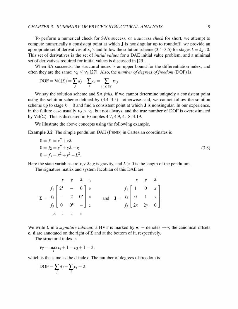
Example 3.2 The simple pendulum DAE (PEND) in Cartesian coordinates is
0 = f1 = x′′+ xλ
0 = f2 = y′′+ yλ −g
0 = f3 = x2 + y2−L2.
(3.8)
Here the state variables are x,y,λ ; g is gravity, and L > 0 is the length of the pendulum.The signature matrix and system Jacobian of this DAE are
Σ =
x y λ ci
f1 2• − 0 0
f2 − 2 0• 0
f3 0 0• − 2
d j 2 2 0
and J =
x y λ
f1 1 0 x
f2 0 1 y
f3 2x 2y 0.
We write Σ in a signature tableau: a HVT is marked by •; − denotes −∞; the canonical offsetsc, d are annotated on the right of Σ and at the bottom of it, respectively.
The structural index is
νS = maxi
ci +1 = c3 +1 = 3,
which is the same as the d-index. The number of degrees of freedom is
DOF = ∑j
d j−∑i
ci = 2.
CHAPTER 3. SUMMARY OF PRYCE’S STRUCTURAL ANALYSIS 10
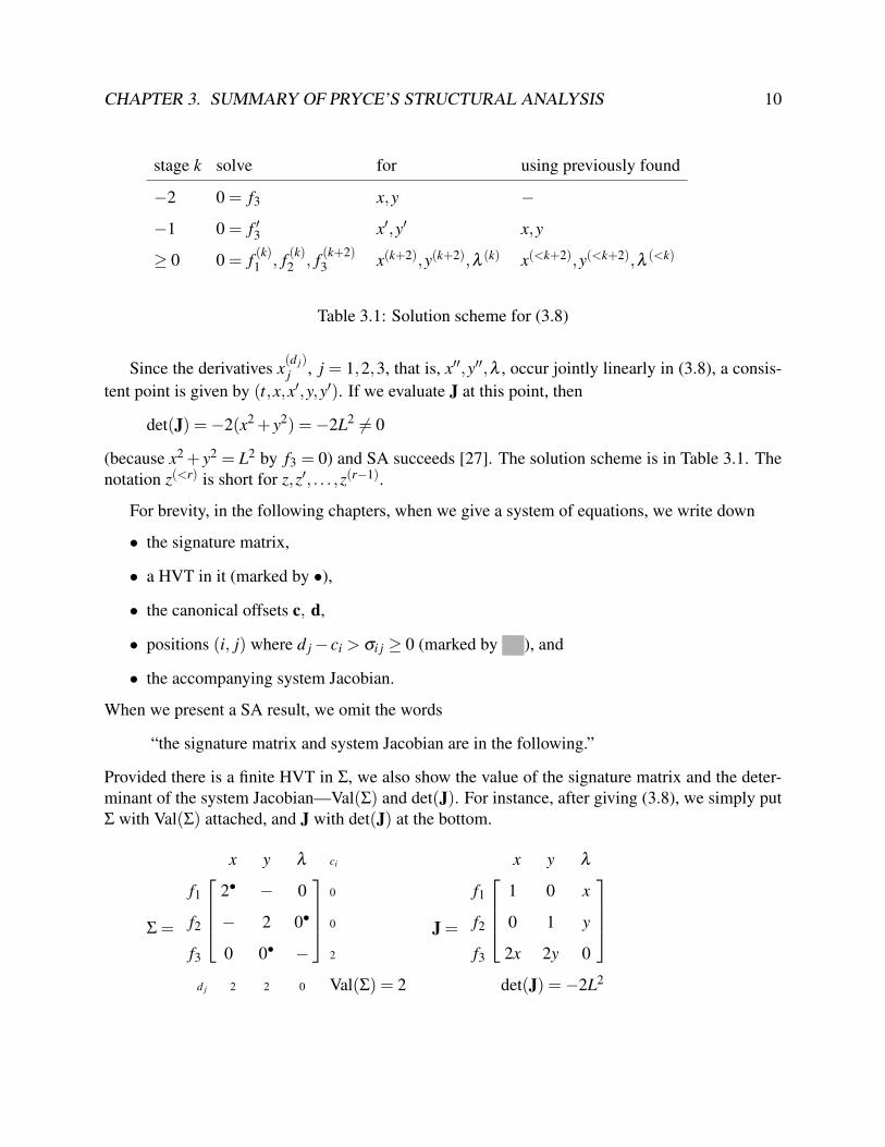
stage k solve for using previously found
−2 0 = f3 x,y −
−1 0 = f ′3 x′,y′ x,y
≥ 0 0 = f (k)1 , f (k)2 , f (k+2)3 x(k+2),y(k+2),λ (k) x(<k+2),y(<k+2),λ (<k)
Table 3.1: Solution scheme for (3.8)
Since the derivatives x(d j)j , j = 1,2,3, that is, x′′,y′′,λ , occur jointly linearly in (3.8), a consis-
tent point is given by (t,x,x′,y,y′). If we evaluate J at this point, then
det(J) =−2(x2 + y2) =−2L2 6= 0
(because x2 + y2 = L2 by f3 = 0) and SA succeeds [27]. The solution scheme is in Table 3.1. Thenotation z(<r) is short for z,z′, . . . ,z(r−1).
For brevity, in the following chapters, when we give a system of equations, we write down
• the signature matrix,
• a HVT in it (marked by •),
• the canonical offsets c, d,
• positions (i, j) where d j− ci > σi j ≥ 0 (marked by ), and
• the accompanying system Jacobian.
When we present a SA result, we omit the words
“the signature matrix and system Jacobian are in the following.”
Provided there is a finite HVT in Σ, we also show the value of the signature matrix and the deter-minant of the system Jacobian—Val(Σ) and det(J). For instance, after giving (3.8), we simply putΣ with Val(Σ) attached, and J with det(J) at the bottom.
Σ =
x y λ ci
f1 2• − 0 0
f2 − 2 0• 0
f3 0 0• − 2
d j 2 2 0 Val(Σ) = 2
J =
x y λ
f1 1 0 x
f2 0 1 y
f3 2x 2y 0
det(J) =−2L2

CHAPTER 3. SUMMARY OF PRYCE’S STRUCTURAL ANALYSIS 11
Similarly, if we write the signature matrix of a system as Σ, then we write correspondinglythe canonical offsets as c, d, and the Jacobian as J. Throughout this report, we shall show DAEproblems for which our conversion methods are suitable. These methods critically depend on theSA results.
Chapter 4
Structural analysis’s failure
In this chapter, we investigate how SA fails on some DAEs. That is, SA produces a singular systemJacobian, and the problem is solvable. In §4.1, we give definitions for (a) a structural zero in thesystem Jacobian, and (b) a structurally singular DAE, where the system Jacobian is identicallysingular. In §4.2 we identify two types of SA’s failure.
4.1 Success checkTo perform a success check for SA on a SWP DAE, we attempt to evaluate the system Jacobian Jin (3.3). If a point (3.6) satisfies the solution scheme (3.4–3.5) at stages k = kd,kd +1, . . . ,0, and Jis nonsingular, then SA succeeds.
In the definitions that follow, we let A be an n×n matrix function.
Definition 4.1 An (i, j) position is a structural zero of A if Ai j is identically 0; otherwise it is astructural nonzero.
Definition 4.2 [20] Matrix A is structurally singular if every B ∈ Rn×n, with Bi j = 0 in A’s struc-tural zero positions, is singular—equivalently, if every transversal of A contains a structural zero.Otherwise A is structurally nonsingular .
Definition 4.3 Matrix A is identically singular, if its determinant is identically 0; otherwise it isgenerically nonsingular.
For a matrix function, being structurally singular is a special case of being identically singular;see Example 4.4 below.
Example 4.4 Consider the following three matrix functions of variables x and y:
A1 =
[x x0 0
], A2 =
[x xy y
], and A3 =
[x yy x
].
12
CHAPTER 4. STRUCTURAL ANALYSIS’S FAILURE 13
A1 is identically singular because det(A1) = 0. It is also structurally singular, since everyB ∈ R2×2 with B21 = B22 = 0 is singular. Here, (2,1) and (2,2) are structural zero positions of A,and each transversal in A contains a structural zero.
A2 is also identically singular, as det(A2) = xy− xy = 0. It is structurally nonsingular, since atransversal does not contain a structural zero.
A3 is structurally nonsingular. It is generically nonsingular, since det(A3) = x2− y2 is notidentically zero. A3 is singular only when x =±y.
In the following, we denote (1.1) by F and define two concepts for it:
• a structural zero in the system Jacobian J, and
• a structurally singular DAE.
Let J be the set of index-pairs
J ={( j, l) | j = 1 : n , l ∈ N
}. (4.1)
Given an n-vector function x = x(t) that is sufficiently smooth (but not necessarily a solution ofF), let
xJ ={
x(l)j | ( j, l) ∈ J}.
For a finite subset J of J , we define a |J|-vector xJ whose components are x(l)j as ( j, l) ranges overJ. (The ordering of these components does not matter.)
Now we denote a DAE as F . We define the derivative set of F as
derset(F) ={( j, l) | x(l)j occurs in F
}. (4.2)
Then the derivatives occurring in F can be denoted concisely as xderset(F).By a value point we mean a ξ ∈ R×R|derset(F)| that contains values for t and values for the
derivative symbols in xderset(F).
Example 4.5 In the simple pendulum DAE (3.8), the state variables x,y,λ are x1,x2,x3. Let L = 5and g = 9.8. Then
derset(F) ={(1,0), (1,2), (2,0), (2,2), (3,0)
}.
A possible value point can be
ξ = (t,x1,x′′1,x2,x′′2,x3) = (2,3,−3,4,1.6,1),
which satisfies f1 and f3 but not f2.
CHAPTER 4. STRUCTURAL ANALYSIS’S FAILURE 14
Similarly, we define the derivative set of J:
derset(J) ={( j, l) | x(l)j occurs in J
}.
From (3.3), a derivative occurring in J must also occur in F , but not vice versa. For example,in PEND, x′′,y′′,λ do not appear in J, and derset(J) =
{(1,0),(2,0)
}; cf. Example 3.2. The
derivative set of J is a subset of that of F : derset(J)⊆ derset(F).
Definition 4.6 An (i, j) position is a structural zero of J, if Ji j is identically zero at all value pointsξ ∈ R×R|derset(F)| that satisfy 0 or more equations from
0 = f (m)i , m≥ 0, i = 1 : n. (4.3)
Otherwise, (i, j) is a structural nonzero.
For the present purpose, we do not require the DAE to have a unique solution, or even anysolution. That is, we do not consider existence and uniqueness of the DAE at this stage, whileidentifying structural zeros of J and the singularity of J discussed below.
Recall (3.3) that defines J. If d j− ci > σi j, then Ji j = 0 and thus position (i, j) is a structuralzero in J. The converse is not true; see Example 4.7.
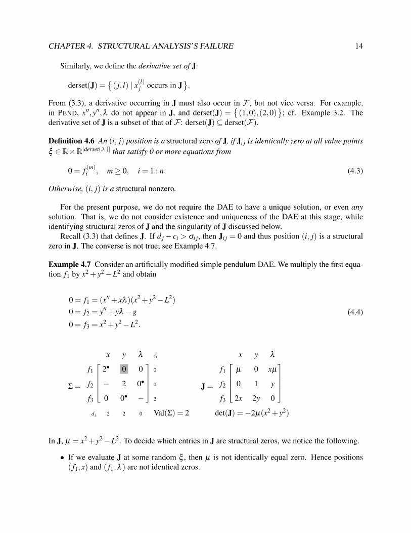
Example 4.7 Consider an artificially modified simple pendulum DAE. We multiply the first equa-tion f1 by x2 + y2−L2 and obtain
0 = f1 = (x′′+ xλ )(x2 + y2−L2)
0 = f2 = y′′+ yλ −g
0 = f3 = x2 + y2−L2.
(4.4)
Σ =
x y λ ci
f1 2• 0 0 0
f2 − 2 0• 0
f3 0 0• − 2
d j 2 2 0 Val(Σ) = 2
J =
x y λ
f1 µ 0 xµ
f2 0 1 y
f3 2x 2y 0
det(J) =−2µ(x2 + y2)
In J, µ = x2 + y2−L2. To decide which entries in J are structural zeros, we notice the following.
• If we evaluate J at some random ξ , then µ is not identically equal zero. Hence positions( f1,x) and ( f1,λ ) are not identical zeros.

CHAPTER 4. STRUCTURAL ANALYSIS’S FAILURE 15
• If we evaluate J at some ξ that satisfies
µ = f3 = x2 + y2−L2 = 0,
then according to Definition 4.6, positions ( f1,x) and ( f1,λ ) are structural zeros of J.
We give a definition for structural regularity of a DAE.
Definition 4.8 A DAE is structurally singular if J is identically singular at all value points ξ ∈R×R|derset(F)| that satisfy 0 or more equations from (4.3). Otherwise the DAE is structurallynonsingular, or structurally regular.
Example 4.9 In the previous example, positions ( f1,x) and ( f1,λ ) are structural zeros of J at anypoint that satisfies f3 = 0. By Definition 4.8, (4.4) is structurally singular.
In fact, it can be shown that a solution of PEND is a solution to (4.4), but not vice versa.
Example 4.10 Consider the DAE in [1, p. 235, Example 9.2], written in (1.1) form:
0 = f1 =−y′1 + y3
0 = f2 = y2(1− y2)
0 = f3 = y1y2 + y3(1− y2)− t.(4.5)
Σ =
y1 y2 y3 ci
f1 1• − 0 0
f2 − 0• − 0
f3 0 0 0• 0
d j 1 0 0 Val(Σ) = 1
J =
y1 y2 y3
f1 −1 0 1
f2 0 1−2y2 0
f3 0 y1− y3 1− y2
det(J) =−(1−2y2)(1− y2)
SA gives νS = 1, and det(J) depends solely on y2. From f2 = 0, either y2 = 0 or y2 = 1. To examineif J is nonsingular, we consider each of the following two cases.
• If y2 = 0, then det(J) =−1 and SA succeeds. In this case (4.5) is of d-index 1.
• If y2 = 1, then det(J) = 0 and SA fails. This failure comes as no surprise because (4.5) isnow of d-index 2 and SA underestimates its index; see the discussion in §2.
Remark 4.11 For a structurally ill-posed (SIP) DAE, there does not exist a finite transversal in itsΣ—every transversal in Σ contains at least one −∞. In this case, there exists no valid offsets c,d,not to mention a system Jacobian that depends on these offsets. In contrast, a structurally singularDAE has valid offsets and a system Jacobian that is identically singular. Hereby we distinguish thedifference between a SIP DAE and a structurally singular DAE.
CHAPTER 4. STRUCTURAL ANALYSIS’S FAILURE 16
Suppose J is generically nonsingular. If J is singular when evaluated at a point along a solution,then we say the DAE is locally unsolvable at this point, and we call it a singularity point. SeeExample 4.12.
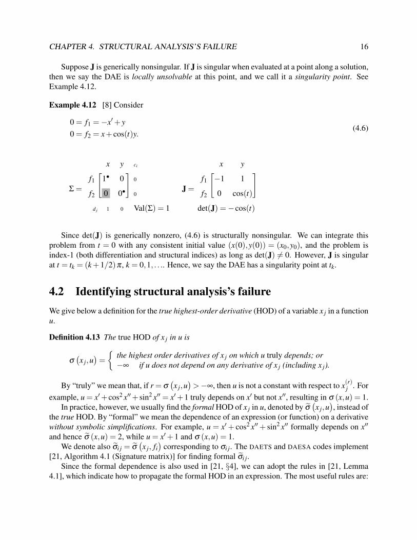
Example 4.12 [8] Consider
0 = f1 =−x′+ y0 = f2 = x+ cos(t)y.
(4.6)
Σ =
x y ci[ ]f1 1• 0 0
f2 0 0• 0
d j 1 0 Val(Σ) = 1
J =
x y[ ]f1 −1 1
f2 0 cos(t)
det(J) =−cos(t)
Since det(J) is generically nonzero, (4.6) is structurally nonsingular. We can integrate thisproblem from t = 0 with any consistent initial value (x(0),y(0)) = (x0,y0), and the problem isindex-1 (both differentiation and structural indices) as long as det(J) 6= 0. However, J is singularat t = tk = (k+1/2)π , k = 0,1, . . .. Hence, we say the DAE has a singularity point at tk.
4.2 Identifying structural analysis’s failureWe give below a definition for the true highest-order derivative (HOD) of a variable x j in a functionu.
Definition 4.13 The true HOD of x j in u is
σ(x j,u
)=
{the highest order derivatives of x j on which u truly depends; or−∞ if u does not depend on any derivative of x j (including x j).
By “truly” we mean that, if r = σ(x j,u
)>−∞, then u is not a constant with respect to x(r)j . For
example, u = x′+cos2 x′′+ sin2 x′′ = x′+1 truly depends on x′ but not x′′, resulting in σ (x,u) = 1.In practice, however, we usually find the formal HOD of x j in u, denoted by σ
(x j,u
), instead of
the true HOD. By “formal” we mean the dependence of an expression (or function) on a derivativewithout symbolic simplifications. For example, u = x′+ cos2 x′′+ sin2 x′′ formally depends on x′′
and hence σ (x,u) = 2, while u = x′+1 and σ (x,u) = 1.We denote also σi j = σ
(x j, fi
)corresponding to σi j. The DAETS and DAESA codes implement
[21, Algorithm 4.1 (Signature matrix)] for finding formal σi j.Since the formal dependence is also used in [21, §4], we can adopt the rules in [21, Lemma
4.1], which indicate how to propagate the formal HOD in an expression. The most useful rules are:
CHAPTER 4. STRUCTURAL ANALYSIS’S FAILURE 17
• if a variable v is a purely algebraic function of a set U of variables u, then
σ(x j,v
)= max
u∈Uσ(x j,u
), (4.7)
and
• if v = dpu/dt p, where p > 0, then
σ(x j,v
)= σ
(x j,u
)+ p. (4.8)
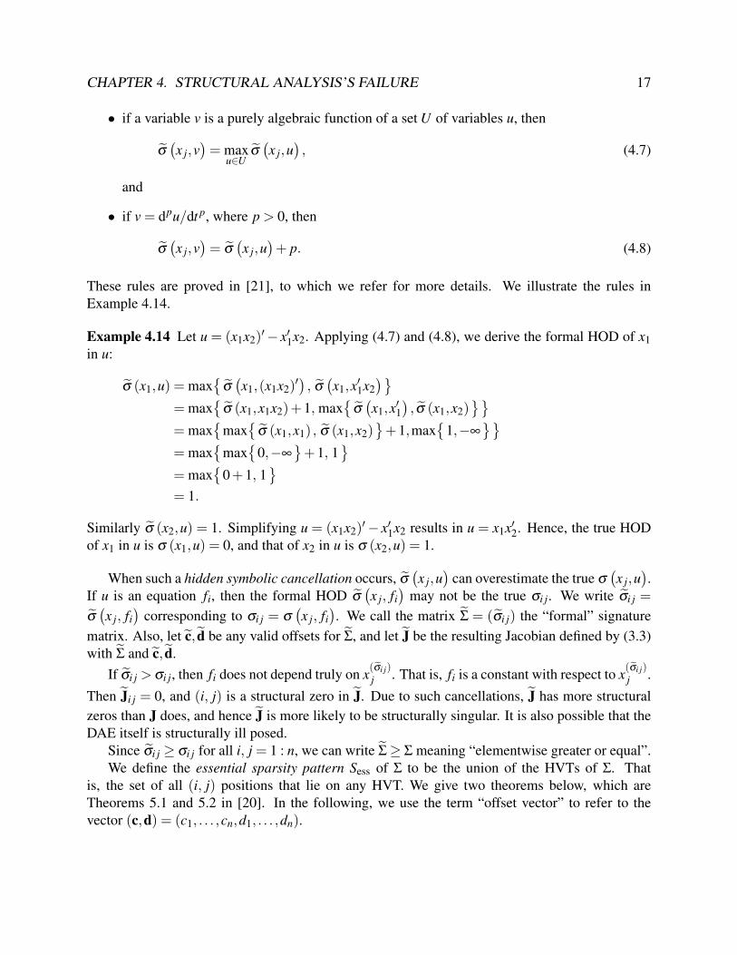
These rules are proved in [21], to which we refer for more details. We illustrate the rules inExample 4.14.
Example 4.14 Let u = (x1x2)′− x′1x2. Applying (4.7) and (4.8), we derive the formal HOD of x1
in u:
σ (x1,u) = max{
σ(x1,(x1x2)
′) , σ(x1,x′1x2
)}= max
{σ (x1,x1x2)+1, max
{σ(x1,x′1
), σ (x1,x2)
}}= max
{max
{σ (x1,x1) , σ (x1,x2)
}+1,max
{1,−∞
}}= max
{max
{0,−∞
}+1, 1
}= max
{0+1, 1
}= 1.
Similarly σ (x2,u) = 1. Simplifying u = (x1x2)′− x′1x2 results in u = x1x′2. Hence, the true HOD
of x1 in u is σ (x1,u) = 0, and that of x2 in u is σ (x2,u) = 1.
When such a hidden symbolic cancellation occurs, σ(x j,u
)can overestimate the true σ
(x j,u
).
If u is an equation fi, then the formal HOD σ(x j, fi
)may not be the true σi j. We write σi j =
σ(x j, fi
)corresponding to σi j = σ
(x j, fi
). We call the matrix Σ = (σi j) the “formal” signature
matrix. Also, let c, d be any valid offsets for Σ, and let J be the resulting Jacobian defined by (3.3)with Σ and c, d.
If σi j > σi j, then fi does not depend truly on x(σi j)j . That is, fi is a constant with respect to x(σi j)
j .
Then Ji j = 0, and (i, j) is a structural zero in J. Due to such cancellations, J has more structuralzeros than J does, and hence J is more likely to be structurally singular. It is also possible that theDAE itself is structurally ill posed.
Since σi j ≥ σi j for all i, j = 1 : n, we can write Σ≥ Σ meaning “elementwise greater or equal”.We define the essential sparsity pattern Sess of Σ to be the union of the HVTs of Σ. That
is, the set of all (i, j) positions that lie on any HVT. We give two theorems below, which areTheorems 5.1 and 5.2 in [20]. In the following, we use the term “offset vector” to refer to thevector (c,d) = (c1, . . . ,cn,d1, . . . ,dn).
CHAPTER 4. STRUCTURAL ANALYSIS’S FAILURE 18
Theorem 4.15 Suppose that a valid offset vector (c,d) for Σ gives a nonsingular J as defined by(3.3) at some consistent point. Then every valid offset vector gives a nonsingular J (not necessarilythe same as J) at this point. All resulting J, including J, are equal on Sess, and all have the samedeterminant det(J) = det(J).
By “equal on Sess” we mean Ji j = Ji j for all (i, j) ∈ Sess.
Theorem 4.16 Assume that J, resulting from Σ and a valid offset vector (c,d), is genericallynonsingular. Let (c, d) be a valid offset vector for the formal signature matrix Σ, and let J be theJacobian resulting from Σ and (c, d). In exact arithmetic, one of the following two alternativesmust occur:
(i) Val(Σ) = Val(Σ). Then every HVT of Σ is a HVT of Σ, and c, d are valid offsets for Σ. Conse-quently, J is also generically nonsingular.
(ii) Val(Σ)> Val(Σ). Then J is structurally singular.
Theorem 4.16 shows that J, resulting from Σ≥ Σ and a valid offset vector (c, d), is either
(1) nonsingular, and SA is using valid, but not necessarily canonical, offsets for the true Σ; or
(2) structurally singular, and SA fails due to symbolic cancellations, in a way that may be detected.
In the latter case, this failure may be avoided by performing symbolic simplification on someor all of the fi’s. However, “no clever symbolic manipulation can overcome the hidden cancella-tion problem, because the task of determining whether some expression is exactly zero is knownto be undecidable in any algebra closed under the basic arithmetic operations together with theexponential function” [20].
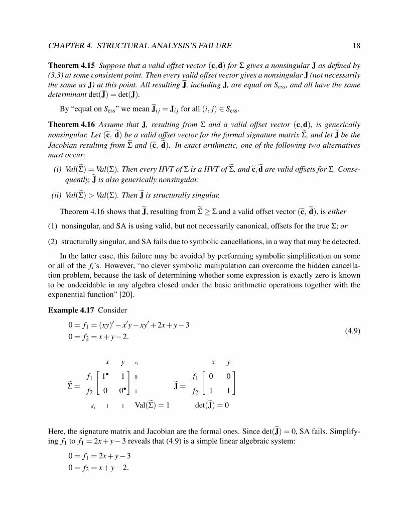
Example 4.17 Consider
0 = f1 = (xy)′− x′y− xy′+2x+ y−30 = f2 = x+ y−2.
(4.9)
Σ =
x y ci[ ]f1 1• 1 0
f2 0 0• 1
d j 1 1 Val(Σ) = 1
J =
x y[ ]f1 0 0
f2 1 1
det(J) = 0
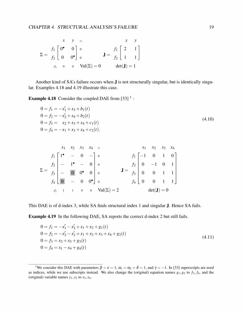
Here, the signature matrix and Jacobian are the formal ones. Since det(J) = 0, SA fails. Simplify-ing f1 to f1 = 2x+ y−3 reveals that (4.9) is a simple linear algebraic system:
0 = f1 = 2x+ y−30 = f2 = x+ y−2.
CHAPTER 4. STRUCTURAL ANALYSIS’S FAILURE 19
Σ =
x y ci[ ]f1 0• 0 0
f2 0 0• 0
d j 0 0 Val(Σ) = 0
J =
x y[ ]f1 2 1
f2 1 1
det(J) = 1
Another kind of SA’s failure occurs when J is not structurally singular, but is identically singu-lar. Examples 4.18 and 4.19 illustrate this case.
Example 4.18 Consider the coupled DAE from [33] 1 :
0 = f1 =−x′1 + x3 +b1(t)0 = f2 =−x′2 + x4 +b2(t)0 = f3 = x2 + x3 + x4 + c1(t)0 = f4 =−x1 + x3 + x4 + c2(t).
(4.10)
Σ =
x1 x2 x3 x4 ci
f1 1• − 0 − 0
f2 − 1• − 0 0
f3 − 0 0• 0 0
f4 0 − 0 0• 0
d j 1 1 0 0 Val(Σ) = 2
J =
x1 x2 x3 x4
f1 −1 0 1 0
f2 0 −1 0 1
f3 0 0 1 1
f4 0 0 1 1
det(J) = 0
This DAE is of d-index 3, while SA finds structural index 1 and singular J. Hence SA fails.
Example 4.19 In the following DAE, SA reports the correct d-index 2 but still fails.
0 = f1 =−x′1− x′3 + x1 + x2 +g1(t)0 = f2 =−x′2− x′3 + x1 + x2 + x3 + x4 +g2(t)0 = f3 = x2 + x3 +g3(t)0 = f4 = x1− x4 +g4(t)
(4.11)
1We consider this DAE with parameters β = ε = 1, α1 = α2 = δ = 1, and γ =−1. In [33] superscripts are usedas indices, while we use subscripts instead. We also change the (original) equation names g1,g2 to f3, f4, and the(original) variable names y1,y2 to x3,x4.
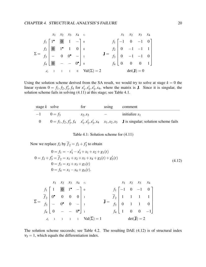
CHAPTER 4. STRUCTURAL ANALYSIS’S FAILURE 20
Σ =
x1 x2 x3 x4 ci
f1 1• 0 1 − 0
f2 0 1• 1 0 0
f3 − 0 0• − 1
f4 0 − − 0• 0
d j 1 1 1 0 Val(Σ) = 2
J =
x1 x2 x3 x4
f1 −1 0 −1 0
f2 0 −1 −1 1
f3 0 −1 −1 0
f4 0 0 0 1
det(J) = 0
Using the solution scheme derived from the SA result, we would try to solve at stage k = 0 thelinear system 0 = f1, f2, f ′3, f4 for x′1,x
′2,x′3,x4, where the matrix is J. Since it is singular, the
solution scheme fails in solving (4.11) at this stage; see Table 4.1.
stage k solve for using comment
−1 0 = f3 x2,x3 − initialize x1
0 0 = f1, f2, f ′3, f4 x′1,x′2,x′3,x4 x1,x2,x3 J is singular; solution scheme fails
Table 4.1: Solution scheme for (4.11)
Now we replace f2 by f 2 = f2 + f ′3 to obtain
0 = f1 =−x′1− x′3 + x1 + x2 +g1(t)
0 = f2 + f ′3 = f 2 = x1 + x2 + x3 + x4 +g2(t)+g′3(t)0 = f3 = x2 + x3 +g3(t)0 = f4 = x1− x4 +g4(t).
(4.12)
Σ =
x1 x2 x3 x4 ci
f1 1 0 1• − 0
f 2 0• 0 0 0 1
f3 − 0• 0 − 1
f4 0 − − 0• 1
d j 1 1 1 1 Val(Σ) = 1
J =
x1 x2 x3 x4
f1 −1 0 −1 0
f 2 1 1 1 1
f3 0 1 1 0
f4 1 0 0 −1
det(J) = 2
The solution scheme succeeds; see Table 4.2. The resulting DAE (4.12) is of structural indexνS = 1, which equals the differentiation index.
CHAPTER 4. STRUCTURAL ANALYSIS’S FAILURE 21
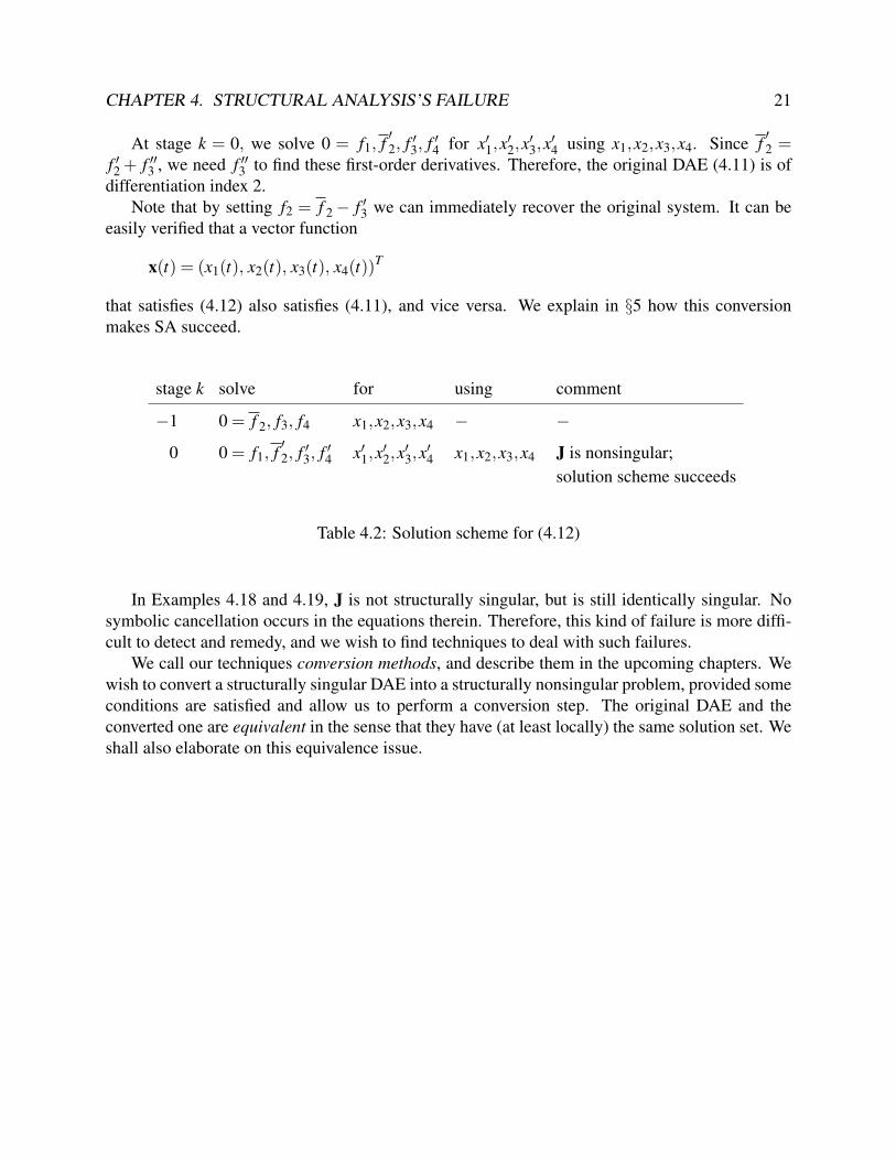
At stage k = 0, we solve 0 = f1, f ′2, f ′3, f ′4 for x′1,x′2,x′3,x′4 using x1,x2,x3,x4. Since f ′2 =
f ′2 + f ′′3 , we need f ′′3 to find these first-order derivatives. Therefore, the original DAE (4.11) is ofdifferentiation index 2.
Note that by setting f2 = f 2− f ′3 we can immediately recover the original system. It can beeasily verified that a vector function
x(t) = (x1(t), x2(t), x3(t), x4(t))T
that satisfies (4.12) also satisfies (4.11), and vice versa. We explain in §5 how this conversionmakes SA succeed.
stage k solve for using comment
−1 0 = f 2, f3, f4 x1,x2,x3,x4 − −
0 0 = f1, f ′2, f ′3, f ′4 x′1,x′2,x′3,x′4 x1,x2,x3,x4 J is nonsingular;
solution scheme succeeds
Table 4.2: Solution scheme for (4.12)
In Examples 4.18 and 4.19, J is not structurally singular, but is still identically singular. Nosymbolic cancellation occurs in the equations therein. Therefore, this kind of failure is more diffi-cult to detect and remedy, and we wish to find techniques to deal with such failures.
We call our techniques conversion methods, and describe them in the upcoming chapters. Wewish to convert a structurally singular DAE into a structurally nonsingular problem, provided someconditions are satisfied and allow us to perform a conversion step. The original DAE and theconverted one are equivalent in the sense that they have (at least locally) the same solution set. Weshall also elaborate on this equivalence issue.
Chapter 5
The linear combination method
In this chapter we introduce the linear combination method, or the LC method for short. We presentin §5.1 some preliminary lemmas. Then we describe in §5.2 how to perform a conversion step. In§5.3 we give definitions and results about equivalence of DAEs and address how equivalence isrelated to the LC method.
For simplicity, throughout this report, we consider only the second type of SA’s failures de-scribed in §4.2: “singular” means identically singular but not structurally singular. Based on thisassumption, symbolic cancellations are not considered an issue that makes the Σ-method fail.
5.1 Preliminary lemmasLemma 5.1 (Griewank’s Lemma) [21, Lemma 5.1] Let v be a function of t, x j’s and derivativesof them ( j = 1 : n). Denote v(p) = dpv/dt p, where p > 0. If σ
(x j,v
)≤ q, then
∂v
∂x(q)j
=∂v′
∂x(q+1)j
.
Hence
∂v
∂x(q)j
=∂v′
∂x(q+1)j
· · ·= ∂v(p)
∂x(q+p)j
. (5.1)
Lemma 5.2 Let Σ and Σ be n×n signature matrices. Assume Val(Σ) is finite, c,d are valid offsetsfor Σ, and σ i j≤ d j−ci for all i, j = 1 : n. If a HVT in Σ contains a position (i, j) where σ i j < d j−ci,then Val(Σ)< Val(Σ).
Proof. Let T be a HVT in Σ. Then
Val(Σ) = ∑(i, j)∈T
σ i j <n
∑j=1
d j−n
∑i=1
ci = Val(Σ). (5.2)
22
CHAPTER 5. THE LINEAR COMBINATION METHOD 23
Corollary 5.3 For a row index l, let{σ i j = σi j for all i 6= l and all j, and
σ l j < d j− cl for all j.
Then Val(Σ)< Val(Σ).
Proof. Since σ l j < d j− cl for all j, the intersection of a HVT in Σ with positions in row l is aposition (l,r) with σ lr < dr− cl . By Lemma 5.2, Val(Σ)< Val(Σ).
This lemma shows that, if we replace a row l in Σ with a row with entries less than d j− cl foreach column j, then the value of this signature matrix decreases.
5.2 Conversion stepGiven a SWP DAE of the form (1.1), assume that we apply the Σ-method and obtain a singularsystem Jacobian J. We seek a reformulation of this DAE so that the system Jacobian J of the newDAE may be generically nonsingular. We denote by Σ and Σ the signature matrices of the originalDAE and this new DAE, respectively. Denote by c,d the valid offsets for Σ.
We describe below how to perform a conversion step using a linear combination (LC) of equa-tions. We call this conversion technique the LC conversion method, or simply the LC method. Themain result from this conversion is that, under certain conditions, we can obtain an equation in arow, say l, such that x j occurs in this row of order < d j− cl for all j. Hence by Corollary 5.3,Val(Σ)< Val(Σ).
We assume n≥ 2. Let u be a nonzero vector function from the null space of JT . Here, J and uare considered as functions of t, x j’s and appropriate derivatives of them.
Denote by I(u) the set of indices for which the ith component of u is not identically zero
I(u) = { i | ui 6= 0}, (5.3)
and let
θ(u) = mini∈I(u)
ci. (5.4)
Since u is nonzero and J is identically singular, I(u) has at least two elements. Otherwise J has arow of identical zeros and is structurally singular.
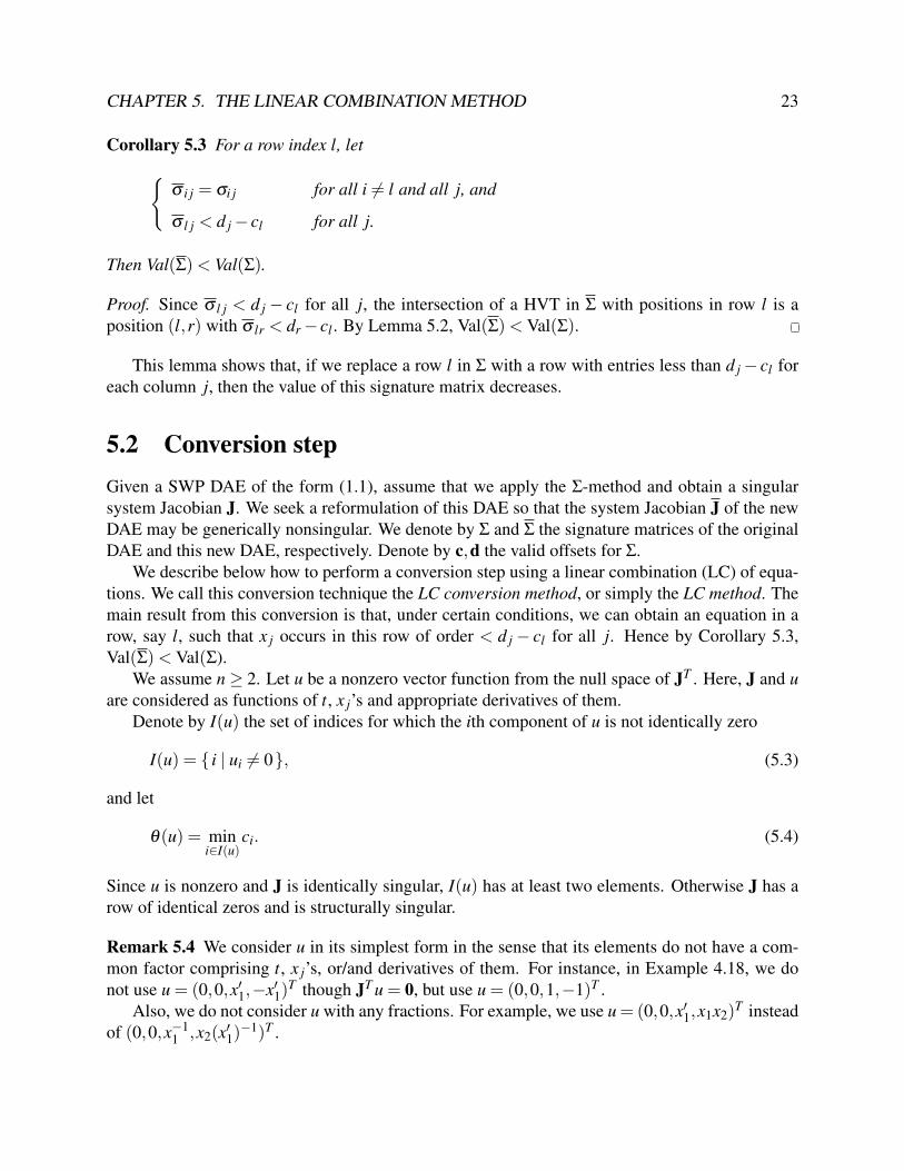
Remark 5.4 We consider u in its simplest form in the sense that its elements do not have a com-mon factor comprising t, x j’s, or/and derivatives of them. For instance, in Example 4.18, we donot use u = (0,0,x′1,−x′1)
T though JT u = 0, but use u = (0,0,1,−1)T .Also, we do not consider u with any fractions. For example, we use u = (0,0,x′1,x1x2)
T insteadof (0,0,x−1
1 ,x2(x′1)−1)T .

CHAPTER 5. THE LINEAR COMBINATION METHOD 24
The sufficient condition for applying the LC method is the following: for a nonzero u∈ ker(JT ),
σ(x j,u
)< d j−θ(u) for all j = 1 : n (5.5)
If this condition is satisfied, then we can perform a conversion step. We explain this “sufficiency”in Remark 5.8.
Denote by L(u) ⊆ I(u) the set of indices l such that the lth component of u is not an identicalzero and cl = θ(u) = mini∈I(u) ci:
L(u) ={
l ∈ I(u) | cl = θ(u)}. (5.6)
From (5.4), there exists at least one l ∈ I(u) such that cl = θ(u), so L(u) 6= /0.We choose an l ∈ L(u) and replace fl by
f l = ∑i∈I(u)
ui f (ci−θ(u))i . (5.7)
We refer to (5.7) as a conversion step using the LC method and to the resulting DAE as a convertedDAE. Critical for the success of the LC method is the following lemma.
Theorem 5.5 For a SWP DAE with identically singular J, let u be a nonzero n-vector such thatJT u = 0. If
σ(x j,u
)< d j−θ(u) for all j = 1 : n
and we replace fl by f l in (5.7), then the converted DAE has Σ with Val(Σ)< Val(Σ).
First, we illustrate with an example how to perform a conversion step, and then we prove thislemma. Since u is fixed during a conversion step, for brevity we write I(u), θ(u), and L(u) as I, θ ,and L, respectively1.
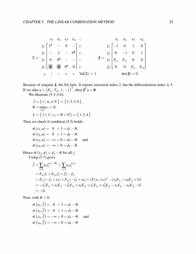
Example 5.6 Consider
0 = f1 =−x′1 + x3
0 = f2 =−x′2 + x4
0 = f3 = F(x1,x2)
0 = f4 = x3Fx1(x1,x2)+ x4Fx2(x1,x2)+G(x1,x2).
(5.8)
Here Fx1(x1,x2) = ∂F(x1,x2)/∂x1, and similarly we write Fx2(x1,x2), Gx1(x1,x2), and Gx2(x1,x2).
1This set L is not to be confused with the constant L in the pendulum-related DAEs.
CHAPTER 5. THE LINEAR COMBINATION METHOD 25
Σ =
x1 x2 x3 x4 ci
f1 1• − 0 − 0
f2 − 1 − 0• 0
f3 0 0• − − 1
f4 0 0 0• 0 0
d j 1 1 0 0 Val(Σ) = 1
J =
x1 x2 x3 x4
f1 −1 0 1 0
f2 0 −1 0 1
f3 Fx1 Fx2 0 0
f4 0 0 Fx1 Fx2
det(J) = 0
Because of singular J, the SA fails. It reports structural index 2, but the differentiation index is 3.If we take u =
(Fx1, Fx2 , 1,−1
)T , then JT u = 0.We illustrate (5.3–5.6):
I ={
i | ui 6= 0}={
1,2,3,4},
θ = mini∈I
ci = 0,
L ={
l ∈ I | cl = θ = 0}={
1,2,4}.
Then we check if condition (5.5) holds:
σ (x1,u) = 0 < 1 = d1−θ ,
σ (x2,u) = 0 < 1 = d2−θ ,
σ (x3,u) =−∞ < 0 = d3−θ , andσ (x4,u) =−∞ < 0 = d4−θ .
Hence σ(x j,u
)< d j−θ for all j.
Using (5.7) gives
f = ∑i∈I
ui f (ci−θ)i = ∑
i∈Iui f (ci)
i
= Fx1 f1 +Fx2 f2 + f ′3− f4
= Fx1(−x′1 + x3)+Fx2(−x′2 + x4)+(F(x1,x2))′− (x3Fx1 + x4Fx2 +G)
=−x′1Fx1 + x3Fx1− x′2Fx2 + x4Fx2 + x′1Fx1 + x′2Fx2− x3Fx1− x4Fx2−G=−G.
Now, with θ = 0,
σ(x1, f
)= 0 < 1 = d1−θ ,
σ(x2, f
)= 0 < 1 = d2−θ ,
σ(x3, f
)=−∞ < 0 = d3−θ , and
σ(x4, f
)=−∞ < 0 = d4−θ .

CHAPTER 5. THE LINEAR COMBINATION METHOD 26
That is, σ(x j, f
)< d j−θ for all j.
For each l ∈ L ={
1,2,4}
, assuming ul 6= 0, we can replace fl by f l = f . We show in thefollowing the three possible converted DAEs, each with Val(Σ) = 0 and generically nonsingular J.
• l = 1:
0 = f 1 =−G(x1,x2)
0 = f2 =−x′2 + x4
0 = f3 = F(x1,x2)
0 = f4 = x3Fx1(x1,x2)+ x4Fx2(x1,x2)+G(x1,x2)
(5.9)
Σ =
x1 x2 x3 x4 ci
f 1 0• 0 − − 1
f2 − 1 − 0• 0
f3 0 0• − − 1
f4 0 0 0• 0 0
d j 1 1 0 0 Val(Σ) = 0
J =
x1 x2 x3 x4
f 1 −Gx1 −Gx2 0 0
f2 0 −1 0 1
f3 Fx1 Fx2 0 0
f4 0 0 Fx1 Fx2
det(J) = Fx1(Fx1Gx2−Fx2Gx1)
When u1 = Fx1 6= 0 and Fx1Gx2 6= Fx2Gx1 , the determinant is nonzero and the SA succeeds.
• l = 2:
0 = f1 =−x′1 + x3
0 = f 2 =−G(x1,x2)
0 = f3 = F(x1,x2)
0 = f4 = x3Fx1(x1,x2)+ x4Fx2(x1,x2)+G(x1,x2)
(5.10)
Σ =
x1 x2 x3 x4 ci
f1 1 − 0• − 0
f 2 0• 0 − − 1
f3 0 0• − − 1
f4 0 0 0 0• 0
d j 1 1 0 0 Val(Σ) = 0
J =
x1 x2 x3 x4
f1 −1 0 1 0
f 2 −Gx1 −Gx2 0 0
f3 Fx1 Fx2 0 0
f4 0 0 Fx1 Fx2
det(J) = Fx2(Fx1Gx2−Fx2Gx1)
Similarly, the SA succeeds when u2 = Fx2 6= 0 and Fx1Gx2 6= Fx2Gx1 .
CHAPTER 5. THE LINEAR COMBINATION METHOD 27
• l = 4:
0 = f1 =−x′1 + x3
0 = f2 =−x′2 + x4
0 = f3 = F(x1,x2)
0 = f 4 =−G(x1,x2)
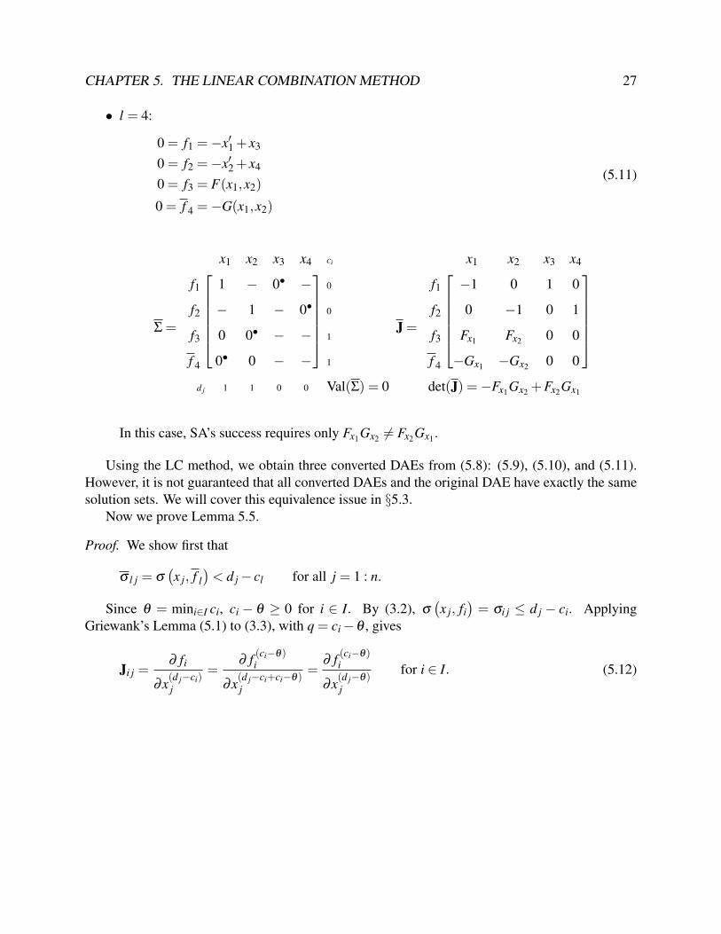
(5.11)
Σ =
x1 x2 x3 x4 ci
f1 1 − 0• − 0
f2 − 1 − 0• 0
f3 0 0• − − 1
f 4 0• 0 − − 1
d j 1 1 0 0 Val(Σ) = 0
J =
x1 x2 x3 x4
f1 −1 0 1 0
f2 0 −1 0 1
f3 Fx1 Fx2 0 0
f 4 −Gx1 −Gx2 0 0
det(J) =−Fx1Gx2 +Fx2Gx1
In this case, SA’s success requires only Fx1Gx2 6= Fx2Gx1 .
Using the LC method, we obtain three converted DAEs from (5.8): (5.9), (5.10), and (5.11).However, it is not guaranteed that all converted DAEs and the original DAE have exactly the samesolution sets. We will cover this equivalence issue in §5.3.
Now we prove Lemma 5.5.
Proof. We show first that
σ l j = σ(x j, f l
)< d j− cl for all j = 1 : n.
Since θ = mini∈I ci, ci − θ ≥ 0 for i ∈ I. By (3.2), σ(x j, fi
)= σi j ≤ d j − ci. Applying
Griewank’s Lemma (5.1) to (3.3), with q = ci−θ , gives
Ji j =∂ fi
∂x(d j−ci)j
=∂ f (ci−θ)
i
∂x(d j−ci+ci−θ)j
=∂ f (ci−θ)
i
∂x(d j−θ)j
for i ∈ I. (5.12)
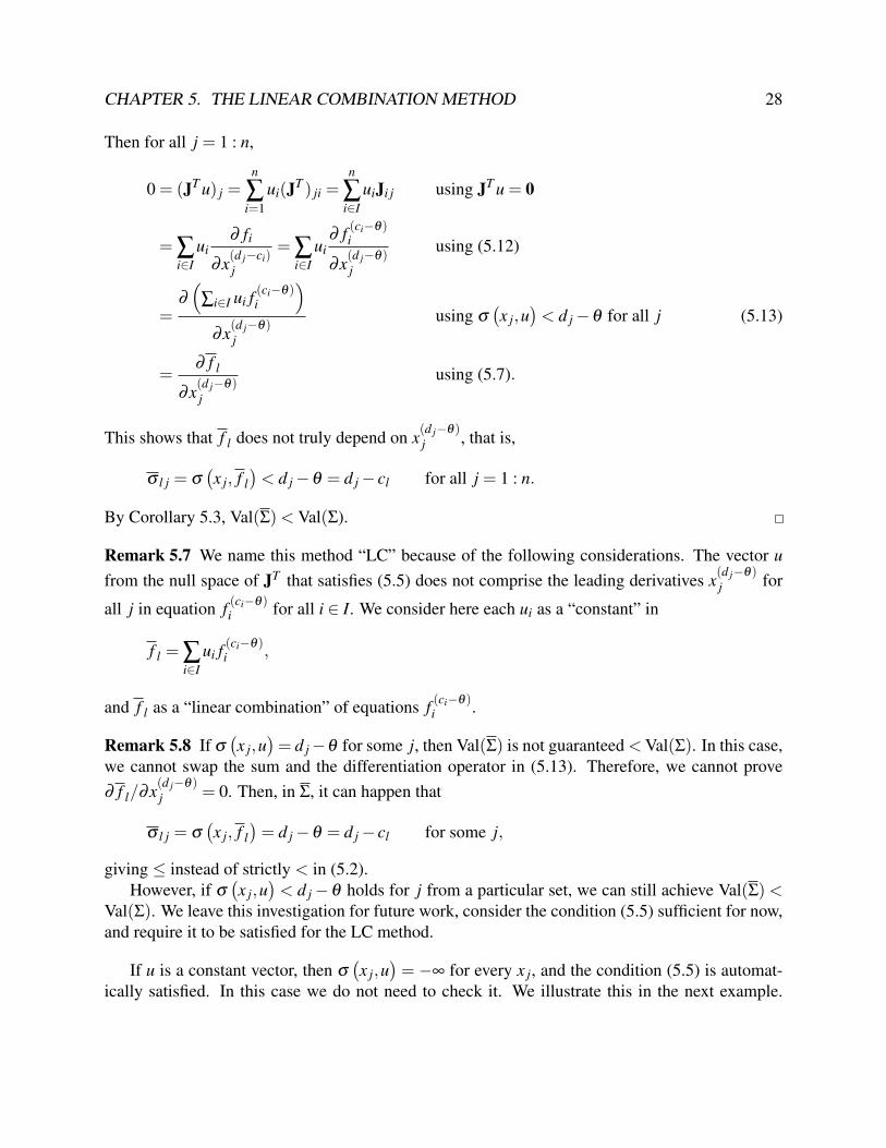
CHAPTER 5. THE LINEAR COMBINATION METHOD 28
Then for all j = 1 : n,
0 = (JT u) j =n
∑i=1
ui(JT ) ji =n
∑i∈I
uiJi j using JT u = 0
= ∑i∈I
ui∂ fi
∂x(d j−ci)j
= ∑i∈I
ui∂ f (ci−θ)
i
∂x(d j−θ)j
using (5.12)
=∂
(∑i∈I ui f (ci−θ)
i
)∂x(d j−θ)
j
using σ(x j,u
)< d j−θ for all j (5.13)
=∂ f l
∂x(d j−θ)j
using (5.7).
This shows that f l does not truly depend on x(d j−θ)j , that is,
σ l j = σ(x j, f l
)< d j−θ = d j− cl for all j = 1 : n.
By Corollary 5.3, Val(Σ)< Val(Σ).
Remark 5.7 We name this method “LC” because of the following considerations. The vector ufrom the null space of JT that satisfies (5.5) does not comprise the leading derivatives x(d j−θ)
j for
all j in equation f (ci−θ)i for all i ∈ I. We consider here each ui as a “constant” in
f l = ∑i∈I
ui f (ci−θ)i ,
and f l as a “linear combination” of equations f (ci−θ)i .
Remark 5.8 If σ(x j,u
)= d j−θ for some j, then Val(Σ) is not guaranteed < Val(Σ). In this case,
we cannot swap the sum and the differentiation operator in (5.13). Therefore, we cannot prove∂ f l/∂x(d j−θ)
j = 0. Then, in Σ, it can happen that
σ l j = σ(x j, f l
)= d j−θ = d j− cl for some j,
giving ≤ instead of strictly < in (5.2).However, if σ
(x j,u
)< d j−θ holds for j from a particular set, we can still achieve Val(Σ) <
Val(Σ). We leave this investigation for future work, consider the condition (5.5) sufficient for now,and require it to be satisfied for the LC method.
If u is a constant vector, then σ(x j,u
)= −∞ for every x j, and the condition (5.5) is automat-
ically satisfied. In this case we do not need to check it. We illustrate this in the next example.
CHAPTER 5. THE LINEAR COMBINATION METHOD 29
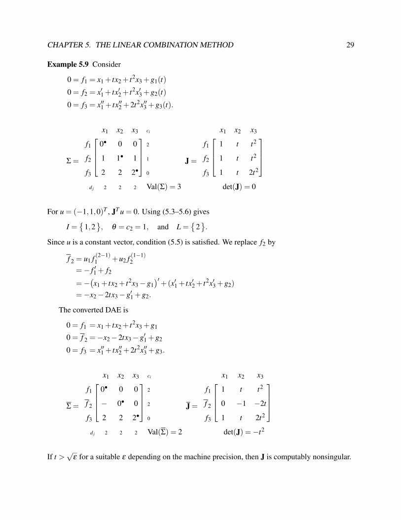
Example 5.9 Consider
0 = f1 = x1 + tx2 + t2x3 +g1(t)
0 = f2 = x′1 + tx′2 + t2x′3 +g2(t)
0 = f3 = x′′1 + tx′′2 +2t2x′′3 +g3(t).
Σ =
x1 x2 x3 ci
f1 0• 0 0 2
f2 1 1• 1 1
f3 2 2 2• 0
d j 2 2 2 Val(Σ) = 3
J =
x1 x2 x3
f1 1 t t2
f2 1 t t2
f3 1 t 2t2
det(J) = 0
For u = (−1,1,0)T , JT u = 0. Using (5.3–5.6) gives
I ={
1,2}, θ = c2 = 1, and L =
{2}.
Since u is a constant vector, condition (5.5) is satisfied. We replace f2 by
f 2 = u1 f (2−1)1 +u2 f (1−1)
2
=− f ′1 + f2
=−(x1 + tx2 + t2x3−g1
)′+(x′1 + tx′2 + t2x′3 +g2)
=−x2−2tx3−g′1 +g2.
The converted DAE is
0 = f1 = x1 + tx2 + t2x3 +g1
0 = f 2 =−x2−2tx3−g′1 +g2
0 = f3 = x′′1 + tx′′2 +2t2x′′3 +g3.
Σ =
x1 x2 x3 ci
f1 0• 0 0 2
f 2 − 0• 0 2
f3 2 2 2• 0
d j 2 2 2 Val(Σ) = 2
J =
x1 x2 x3
f1 1 t t2
f 2 0 −1 −2t
f3 1 t 2t2
det(J) =−t2
If t >√
ε for a suitable ε depending on the machine precision, then J is computably nonsingular.
CHAPTER 5. THE LINEAR COMBINATION METHOD 30
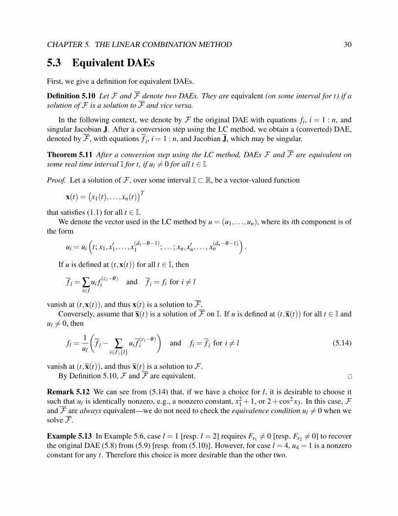
5.3 Equivalent DAEsFirst, we give a definition for equivalent DAEs.
Definition 5.10 Let F and F denote two DAEs. They are equivalent (on some interval for t) if asolution of F is a solution to F and vice versa.
In the following context, we denote by F the original DAE with equations fi, i = 1 : n, andsingular Jacobian J. After a conversion step using the LC method, we obtain a (converted) DAE,denoted by F , with equations f i, i = 1 : n, and Jacobian J, which may be singular.
Theorem 5.11 After a conversion step using the LC method, DAEs F and F are equivalent onsome real time interval I for t, if ul 6= 0 for all t ∈ I.
Proof. Let a solution of F , over some interval I⊂ R, be a vector-valued function
x(t) =(x1(t), . . . ,xn(t)
)T
that satisfies (1.1) for all t ∈ I.We denote the vector used in the LC method by u = (u1, . . . ,un), where its ith component is of
the form
ui = ui
(t; x1,x′1, . . . ,x
(d1−θ−1)1 ; . . . ; xn,x′n, . . . , x(dn−θ−1)
n
).
If u is defined at (t,x(t)) for all t ∈ I, then
f l = ∑i∈I
ui f (ci−θ)i and f i = fi for i 6= l
vanish at (t,x(t)), and thus x(t) is a solution to F .Conversely, assume that x(t) is a solution of F on I. If u is defined at (t,x(t)) for all t ∈ I and
ul 6= 0, then
fl =1ul
(f l− ∑
i∈I\{l}ui f (ci−θ)
i
)and fi = f i for i 6= l (5.14)
vanish at (t,x(t)), and thus x(t) is a solution to F .By Definition 5.10, F and F are equivalent.
Remark 5.12 We can see from (5.14) that, if we have a choice for l, it is desirable to choose itsuch that ul is identically nonzero, e.g., a nonzero constant, x2
1 +1, or 2+ cos2 x3. In this case, Fand F are always equivalent—we do not need to check the equivalence condition ul 6= 0 when wesolve F .
Example 5.13 In Example 5.6, case l = 1 [resp. l = 2] requires Fx1 6= 0 [resp. Fx2 6= 0] to recoverthe original DAE (5.8) from (5.9) [resp. from (5.10)]. However, for case l = 4, u4 = 1 is a nonzeroconstant for any t. Therefore this choice is more desirable than the other two.
CHAPTER 5. THE LINEAR COMBINATION METHOD 31
Below we define an ill-posed DAE using the structural posedness defined in the DAESA papers[23, 29].
Definition 5.14 A DAE is ill posed if it has an equivalent DAE that is structurally ill-posed (SIP);otherwise it is well posed.
Example 5.15 Consider problem (4.4). Using 0 = f3 = x2 + y2−L2, we reduce f1 to the trivial0 = f 1 = 0. This is just performing a simple substitution, and is not applying the LC method. Thesignature matrix
Σ =
x y λ
f 1 − − −
f2 − 2 0
f3 0 0 −
(5.15)
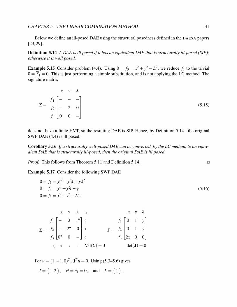
does not have a finite HVT, so the resulting DAE is SIP. Hence, by Definition 5.14 , the originalSWP DAE (4.4) is ill posed.
Corollary 5.16 If a structurally well-posed DAE can be converted, by the LC method, to an equiv-alent DAE that is structurally ill-posed, then the original DAE is ill posed.
Proof. This follows from Theorem 5.11 and Definition 5.14.
Example 5.17 Consider the following SWP DAE
0 = f1 = y′′′+ y′λ + yλ′
0 = f2 = y′′+ yλ −g
0 = f3 = x2 + y2−L2.
(5.16)
Σ =
x y λ ci
f1 − 3 1• 0
f2 − 2• 0 1
f3 0• 0 − 0
d j 0 3 1 Val(Σ) = 3
J =
x y λ
f1 0 1 y
f2 0 1 y
f3 2x 0 0
det(J) = 0
For u = (1,−1,0)T , JT u = 0. Using (5.3–5.6) gives
I ={
1,2}, θ = c1 = 0, and L =
{1}.

CHAPTER 5. THE LINEAR COMBINATION METHOD 32
Since u is a constant vector, condition (5.5) is satisfied. We replace f1 by
f 1 = f1− f ′2 = (y′′′+ y′λ + yλ′)− (y′′+ yλ −g)′ = 0.
The signature matrix of the resulting problem is exactly (5.15). Hence, by Corollary 5.16, (5.16)is ill posed.
If the Jacobian of the converted DAE is still singular, we may be able to apply the LC methoditeratively, provided condition (5.5) is satisfied on each iteration. Since after each conversion stepwe reduce the value of the signature matrix by at least 1, the number of iterations does not exceedVal(Σ), where Σ is for the original DAE. We use Example 5.18 to show how we can iterate withthe LC method.
Example 5.18 We construct the following (artificial) MODPENDA DAE from PEND (3.8):
0 = A = f3 + f ′1 = x2 + y2−L2 +(x′′+ xλ )′
0 = B = f1 +A′′ = x′′+ xλ +(x2 + y2−L2 +(x′′+ xλ )′
)′′0 =C = f2 +A′′′ = y′′+ yλ −g+
(x2 + y2−L2 +(x′′+ xλ )′
)′′′.
(5.17)
Σ0 =
x y λ ci
A 3• 0 1 3
B 5 2• 3 1
C 6 3 4• 0
d j 6 3 4 Val(Σ0) = 9
J0 =
x y λ
A 1 2y x
B 1 2y x
C 1 2y x
det(J0) = 0
Here, a superscript denotes an iteration number, not a power. We show how to recover the simplependulum problem.
We find a vector in ker((J0)T ): u0 = (−1,1,0)T . Then
I0 ={
1,2}, θ
0 = 1, and L0 ={
2}.
We replace the second equation B by
−A(3−1)+B =−A′′+(A′′+ f1) = f1 = x′′+ xλ .
The converted DAE is
0 = A = x2 + y2−L2 +(x′′+ xλ )′
0 = f1 = x′′+ xλ
0 =C = y′′+ yλ −g+(x2 + y2−L2 +(x′′+ xλ )′
)′′′.
CHAPTER 5. THE LINEAR COMBINATION METHOD 33
Σ1 =
x y λ ci
A 3• 0 1 3
f1 2 − 0• 4
C 6 3• 4 0
d j 6 3 4 Val(Σ1) = 6
J1 =
x y λ
A 1 2y x
f1 1 0 x
C 1 2y x
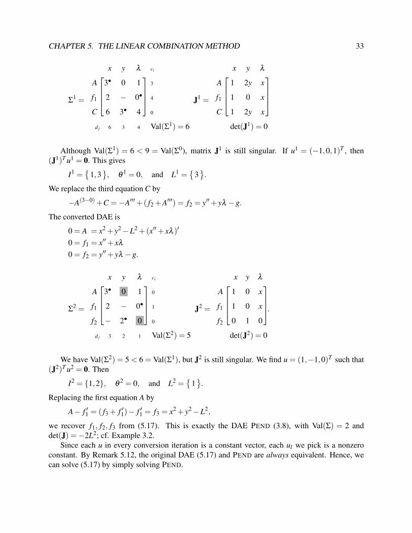
det(J1) = 0
Although Val(Σ1) = 6 < 9 = Val(Σ0), matrix J1 is still singular. If u1 = (−1,0,1)T , then(J1)T u1 = 0. This gives
I1 ={
1,3}, θ
1 = 0, and L1 ={
3}.
We replace the third equation C by
−A(3−0)+C =−A′′′+( f2 +A′′′) = f2 = y′′+ yλ −g.
The converted DAE is
0 = A = x2 + y2−L2 +(x′′+ xλ )′
0 = f1 = x′′+ xλ
0 = f2 = y′′+ yλ −g.
Σ2 =
x y λ ci
A 3• 0 1 0
f1 2 − 0• 1
f2 − 2• 0 0
d j 3 2 1 Val(Σ2) = 5
J2 =
x y λ
A 1 0 x
f1 1 0 x
f2 0 1 0
det(J2) = 0
.
We have Val(Σ2) = 5 < 6 = Val(Σ1), but J2 is still singular. We find u = (1,−1,0)T such that(J2)T u2 = 0. Then
I2 = {1,2}, θ2 = 0, and L2 =
{1}.
Replacing the first equation A by
A− f ′1 = ( f3 + f ′1)− f ′1 = f3 = x2 + y2−L2,
we recover f1, f2, f3 from (5.17). This is exactly the DAE PEND (3.8), with Val(Σ) = 2 anddet(J) =−2L2; cf. Example 3.2.
Since each u in every conversion iteration is a constant vector, each ul we pick is a nonzeroconstant. By Remark 5.12, the original DAE (5.17) and PEND are always equivalent. Hence, wecan solve (5.17) by simply solving PEND.

Chapter 6
The expression substitution method
We develop in this chapter the expression substitution conversion method. In §6.1, we introducesome notation. We describe in §6.2 how to perform a conversion step using this method and addressin §6.3 the equivalence issue.
6.1 PreliminariesA conversion using the LC method seeks a row in Σ, replaces the corresponding equation by alinear combination of existing equations, and constructs a new DAE with a signature matrix of asmaller value. Inspired by the LC method, our goal is to develop a conversion method that seeksa column in Σ, performs a change of certain variables, and constructs a new DAE with Σ such thatVal(Σ)< Val(Σ). We refer to this approach as the expression substitution (ES) conversion method,or the ES method.
Again, we start from a SWP DAE with a signature matrix Σ, offsets c, d, and identically singu-lar Jacobian J. To start our analysis, we give some notation below.
Let u be a vector function from the null space of J, that is, Ju = 0. Denote by L(u) the set ofindices j for which the jth component of u is not identically zero
L(u) ={
j | u j 6= 0}, (6.1)
and denote s(u) by the number of elements in L(u):
s(u) = |L(u)|. (6.2)
Note that s ≥ 2. Otherwise J has a column that is identically the zero vector, and hence J isstructurally singular.
Let
I(u) ={
i | d j− ci = σi j for some j ∈ L(u)}. (6.3)
34
CHAPTER 6. THE EXPRESSION SUBSTITUTION METHOD 35
Denote also
C(u) = maxi∈I(u)
ci. (6.4)
Now we illustrate (6.1-6.4).
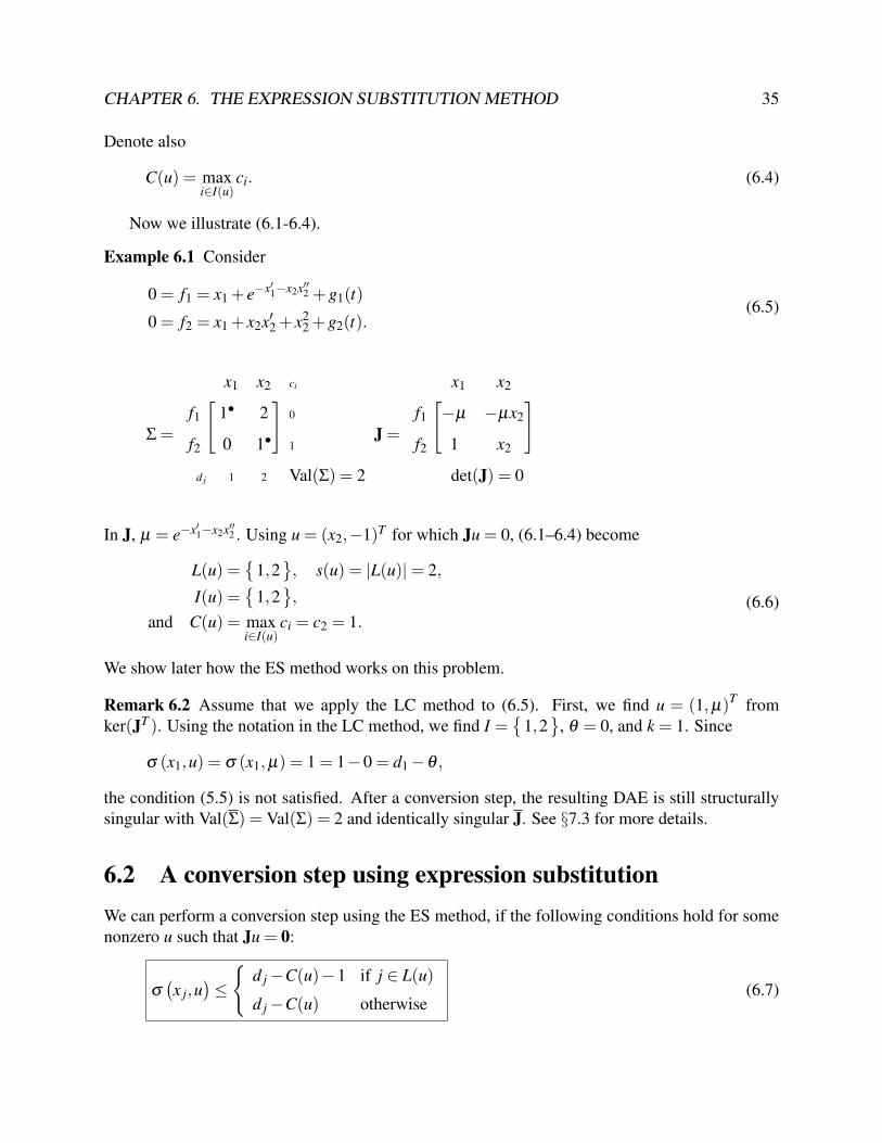
Example 6.1 Consider
0 = f1 = x1 + e−x′1−x2x′′2 +g1(t)
0 = f2 = x1 + x2x′2 + x22 +g2(t).
(6.5)
Σ =
x1 x2 ci[ ]f1 1• 2 0
f2 0 1• 1
d j 1 2 Val(Σ) = 2
J =
x1 x2[ ]f1 −µ −µx2
f2 1 x2
det(J) = 0
In J, µ = e−x′1−x2x′′2 . Using u = (x2,−1)T for which Ju = 0, (6.1–6.4) become
L(u) ={
1,2}, s(u) = |L(u)|= 2,
I(u) ={
1,2},
and C(u) = maxi∈I(u)
ci = c2 = 1.(6.6)
We show later how the ES method works on this problem.
Remark 6.2 Assume that we apply the LC method to (6.5). First, we find u = (1,µ)T fromker(JT ). Using the notation in the LC method, we find I =
{1,2}
, θ = 0, and k = 1. Since
σ (x1,u) = σ (x1,µ) = 1 = 1−0 = d1−θ ,
the condition (5.5) is not satisfied. After a conversion step, the resulting DAE is still structurallysingular with Val(Σ) = Val(Σ) = 2 and identically singular J. See §7.3 for more details.
6.2 A conversion step using expression substitutionWe can perform a conversion step using the ES method, if the following conditions hold for somenonzero u such that Ju = 0:
σ(x j,u
)≤
{d j−C(u)−1 if j ∈ L(u)
d j−C(u) otherwise(6.7)
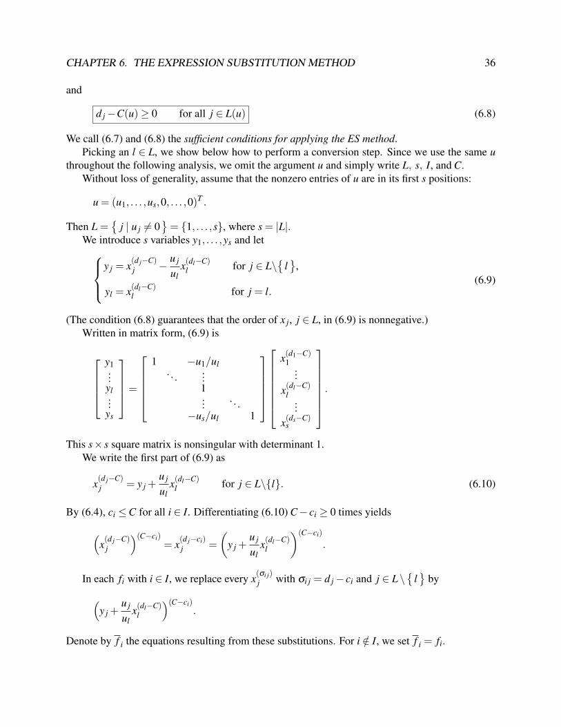
CHAPTER 6. THE EXPRESSION SUBSTITUTION METHOD 36
and
d j−C(u)≥ 0 for all j ∈ L(u) (6.8)
We call (6.7) and (6.8) the sufficient conditions for applying the ES method.Picking an l ∈ L, we show below how to perform a conversion step. Since we use the same u
throughout the following analysis, we omit the argument u and simply write L, s, I, and C.Without loss of generality, assume that the nonzero entries of u are in its first s positions:
u = (u1, . . . ,us,0, . . . ,0)T .
Then L ={
j | u j 6= 0}= {1, . . . ,s}, where s = |L|.
We introduce s variables y1, . . . ,ys and lety j = x(d j−C)
j −u j
ulx(dl−C)
l for j ∈ L\{
l}
,
yl = x(dl−C)l for j = l.
(6.9)
(The condition (6.8) guarantees that the order of x j, j ∈ L, in (6.9) is nonnegative.)Written in matrix form, (6.9) is
y1...yl...
ys
=
1 −u1/ul
. . . ...1... . . .
−us/ul 1
x(d1−C)
1 ...x(dl−C)
l...
x(ds−C)s
.
This s× s square matrix is nonsingular with determinant 1.We write the first part of (6.9) as
x(d j−C)j = y j +
u j
ulx(dl−C)
l for j ∈ L\{l}. (6.10)
By (6.4), ci ≤C for all i ∈ I. Differentiating (6.10) C− ci ≥ 0 times yields(x(d j−C)
j
)(C−ci)= x(d j−ci)
j =
(y j +
u j
ulx(dl−C)
l
)(C−ci)
.
In each fi with i ∈ I, we replace every x(σi j)j with σi j = d j− ci and j ∈ L\
{l}
by(y j +
u j
ulx(dl−C)
l
)(C−ci).
Denote by f i the equations resulting from these substitutions. For i /∈ I, we set f i = fi.
CHAPTER 6. THE EXPRESSION SUBSTITUTION METHOD 37
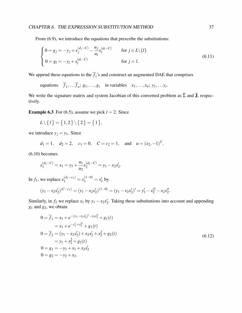
From (6.9), we introduce the equations that prescribe the substitutions:0 = g j =−y j + x(d j−C)
j −u j
ulx(dl−C)
l for j ∈ L\{l}
0 = gl =−yl + x(dl−C)l for j = l.
(6.11)
We append these equations to the f i’s and construct an augmented DAE that comprises
equations f 1, . . . f n; g1, . . . ,gs in variables x1, . . . ,xn; y1, . . .ys.
We write the signature matrix and system Jacobian of this converted problem as Σ and J, respec-tively.
Example 6.3 For (6.5), assume we pick l = 2. Since
L\{
l}={
1,2}\{
2}={
1},
we introduce y j = y1. Since
d1 = 1, d2 = 2, c1 = 0, C = c2 = 1, and u = (x2,−1)T ,
(6.10) becomes
x(d1−C)1 = x1 = y1 +
u1
u2x(d2−C)
2 = y1− x2x′2.
In f1, we replace x(d1−c1)1 = x(1−0)
1 = x′1 by
(y1− x2x′2)(C−c1) = (y1− x2x′2)
(1−0) = (y1− x2x′2)′ = y′1− x′22 − x2x′′2.
Similarly, in f2 we replace x1 by y1− x2x′2. Taking these substitutions into account and appendingg1 and g2, we obtain
0 = f 1 = x1 + e−(y1−x2x′2)′−x2x′′2 +g1(t)
= x1 + e−y′1+x′22 +g1(t)
0 = f 2 = (y1− x2x′2)+ x2x′2 + x22 +g2(t)
= y1 + x22 +g2(t)
0 = g1 =−y1 + x1 + x2x′20 = g2 =−y2 + x2.
(6.12)
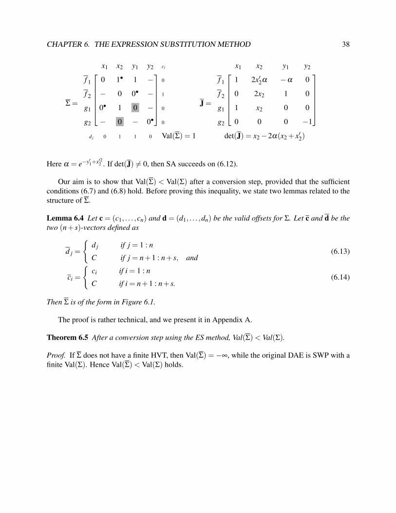
CHAPTER 6. THE EXPRESSION SUBSTITUTION METHOD 38
Σ =
x1 x2 y1 y2 ci
f 1 0 1• 1 − 0
f 2 − 0 0• − 1
g1 0• 1 0 − 0
g2 − 0 − 0• 0
d j 0 1 1 0 Val(Σ) = 1
J =
x1 x2 y1 y2
f 1 1 2x′2α −α 0
f 2 0 2x2 1 0
g1 1 x2 0 0
g2 0 0 0 −1
det(J) = x2−2α(x2 + x′2)
Here α = e−y′1+x′22 . If det(J) 6= 0, then SA succeeds on (6.12).
Our aim is to show that Val(Σ) < Val(Σ) after a conversion step, provided that the sufficientconditions (6.7) and (6.8) hold. Before proving this inequality, we state two lemmas related to thestructure of Σ.
Lemma 6.4 Let c = (c1, . . . ,cn) and d = (d1, . . . ,dn) be the valid offsets for Σ. Let c and d be thetwo (n+ s)-vectors defined as
d j =
{d j if j = 1 : n
C if j = n+1 : n+ s, and(6.13)
ci =
{ci if i = 1 : n
C if i = n+1 : n+ s.(6.14)
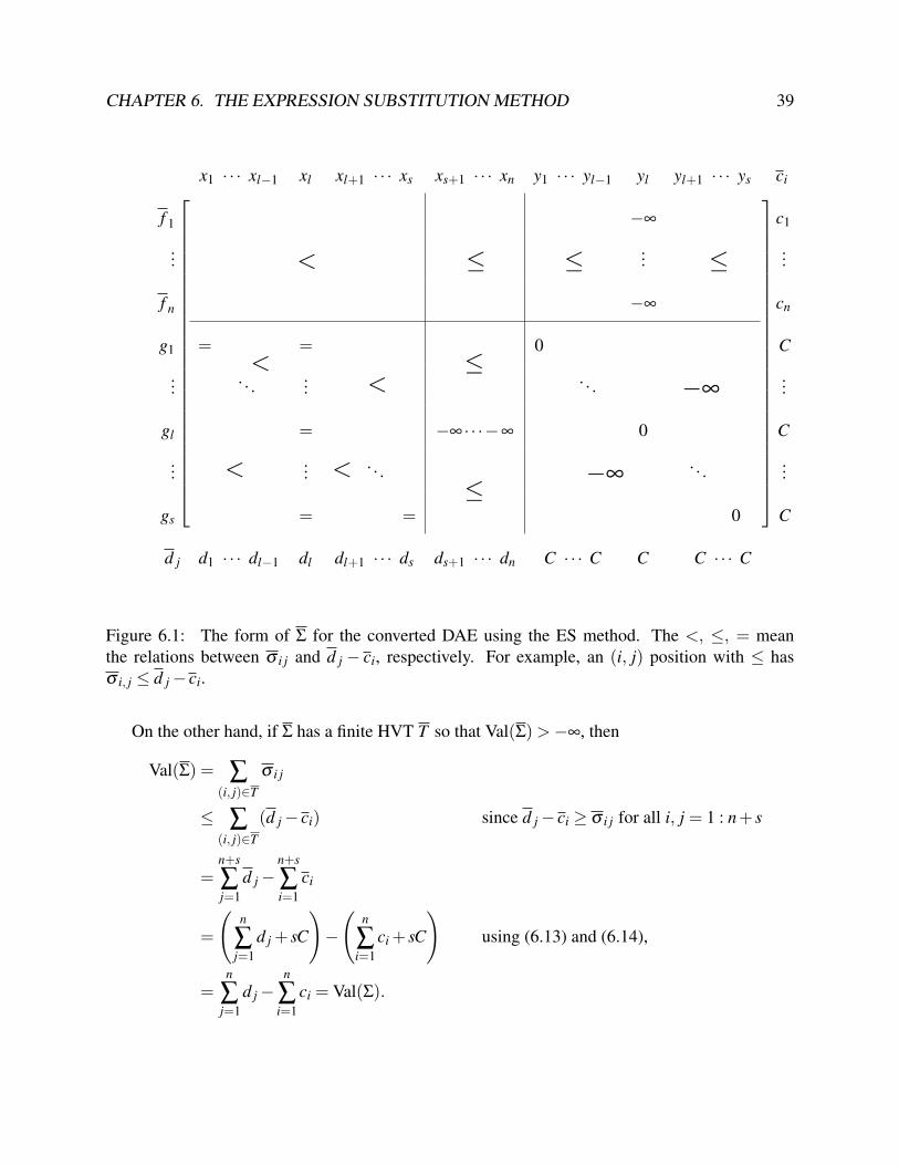
Then Σ is of the form in Figure 6.1.
The proof is rather technical, and we present it in Appendix A.
Theorem 6.5 After a conversion step using the ES method, Val(Σ)< Val(Σ).
Proof. If Σ does not have a finite HVT, then Val(Σ) =−∞, while the original DAE is SWP with afinite Val(Σ). Hence Val(Σ)< Val(Σ) holds.
CHAPTER 6. THE EXPRESSION SUBSTITUTION METHOD 39
x1 · · · xl−1 xl xl+1 · · · xs xs+1 · · · xn y1 · · · yl−1 yl yl+1 · · · ys ci
f 1 −∞ c1
... < ≤ ≤ ... ≤ ...
f n −∞ cn
g1 =<
=
<≤
0 C
... . . . ... . . . −∞...
gl = −∞ · · ·−∞ 0 C
... < ... . . .≤ −∞
. . . ...
gs =
<
= 0 C
d j d1 · · · dl−1 dl dl+1 · · · ds ds+1 · · · dn C · · · C C C · · · C
Figure 6.1: The form of Σ for the converted DAE using the ES method. The <, ≤, = meanthe relations between σ i j and d j − ci, respectively. For example, an (i, j) position with ≤ hasσ i, j ≤ d j− ci.
On the other hand, if Σ has a finite HVT T so that Val(Σ)>−∞, then
Val(Σ) = ∑(i, j)∈T
σ i j
≤ ∑(i, j)∈T
(d j− ci) since d j− ci ≥ σ i j for all i, j = 1 : n+ s
=n+s
∑j=1
d j−n+s
∑i=1
ci
=
(n
∑j=1
d j + sC
)−
(n
∑i=1
ci + sC
)using (6.13) and (6.14),
=n
∑j=1
d j−n
∑i=1
ci = Val(Σ).
CHAPTER 6. THE EXPRESSION SUBSTITUTION METHOD 40
We prove in the following that Val(Σ) = Val(Σ) leads to a contradiction. Assume this equalityholds. Then there exists a transversal T of (n+ s) positions in Σ such that
d j− ci = σ i j >−∞ for all (i, j) ∈ T . (6.15)
The column corresponding to yl has only one finite entry σn+l,n+l = 0, and therefore(n+ l,n+ l) ∈ T . Consider (i1,1), . . . ,(is,s) ∈ T . Since (n+ l,n+ l) ∈ T , row numbers i1, . . . , istake values among
1, 2, . . . , n, n+1, . . . , n+ l−1, n+ l +1, . . . , n+ s. (6.16)
In (6.16) only s− 1 numbers are greater than n. Hence at least one of these row numbers isamong 1 : n. That is, there exists (ir,r) ∈ T with 1 ≤ ir ≤ n and 1 ≤ r ≤ s. This entry is inΣ(1 : n,1 : s)1 in Figure 6.1, so dr − cir > σ ir,r, which contradicts to our assumption in (6.15).Therefore Val(Σ)< Val(Σ).
Remark 6.6 We give several remarks about the ES method.
• After a conversion step, we perform symbolic simplifications on f i, for i ∈ I. By doing thiswe ensure that the x(d j−ci)
j ’s for j ∈ L = {1, . . . ,s} disappear from these equations. That is,σ(x j, f i
)< d j− ci for j = 1 : s and i ∈ I.
• Clearly, yl appears only in gl . We mark down the positions in T on Σ, and then remove rown+ l (corresponding to gl) and column n+ l (corresponding to yl). Because (n+ l,n+ l)∈ T ,the remaining marked positions still form a HVT T in the resulting (n+ s−1)× (n+ s−1)signature matrix Σ.
Since σn+l,n+l = 0, Val(Σ) = Val(Σ). The purpose to use gl and yl in the above proof andanalysis is for our convenience. In practice, we can exclude gl and yl in the resulting DAE.For consistency, after removing gl and yl , we still use Σ and T to denote the signature matrixand system Jacobian, respectively, for the resulting DAE. See Example 6.7.
• If some derivative x(d j−ci)j , for i = 1 : n and j ∈ L\
{l}
, appears implicitly in an expression
in fi, then we need to write this expression into a form in which x(d j−ci)j appears explicitly.
See Example 6.8.
1Using MATLAB notation.
CHAPTER 6. THE EXPRESSION SUBSTITUTION METHOD 41
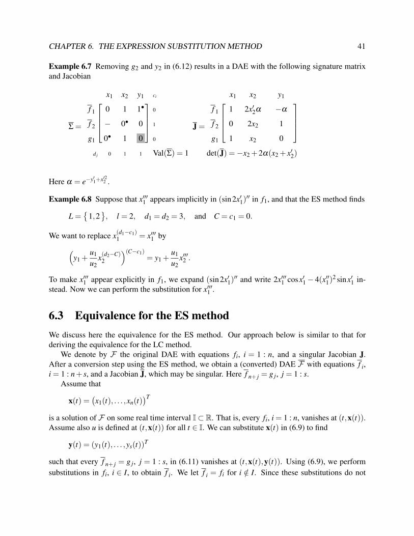
Example 6.7 Removing g2 and y2 in (6.12) results in a DAE with the following signature matrixand Jacobian
Σ =
x1 x2 y1 ci
f 1 0 1 1• 0
f 2 − 0• 0 1
g1 0• 1 0 0
d j 0 1 1 Val(Σ) = 1
J =
x1 x2 y1
f 1 1 2x′2α −α
f 2 0 2x2 1
g1 1 x2 0
det(J) =−x2 +2α(x2 + x′2)
Here α = e−y′1+x′22 .
Example 6.8 Suppose that x′′′1 appears implicitly in (sin2x′1)′′ in f1, and that the ES method finds
L ={
1,2}, l = 2, d1 = d2 = 3, and C = c1 = 0.
We want to replace x(d1−c1)1 = x′′′1 by(
y1 +u1
u2x(d2−C)
2
)(C−c1)= y1 +
u1
u2x′′′2 .
To make x′′′1 appear explicitly in f1, we expand (sin2x′1)′′ and write 2x′′′1 cosx′1− 4(x′′1)
2 sinx′1 in-stead. Now we can perform the substitution for x′′′1 .
6.3 Equivalence for the ES methodWe discuss here the equivalence for the ES method. Our approach below is similar to that forderiving the equivalence for the LC method.
We denote by F the original DAE with equations fi, i = 1 : n, and a singular Jacobian J.After a conversion step using the ES method, we obtain a (converted) DAE F with equations f i,i = 1 : n+ s, and a Jacobian J, which may be singular. Here f n+ j = g j, j = 1 : s.
Assume that
x(t) =(x1(t), . . . ,xn(t)
)T
is a solution of F on some real time interval I⊂R. That is, every fi, i = 1 : n, vanishes at (t,x(t)).Assume also u is defined at (t,x(t)) for all t ∈ I. We can substitute x(t) in (6.9) to find
y(t) = (y1(t), . . . ,ys(t))T
such that every f n+ j = g j, j = 1 : s, in (6.11) vanishes at (t,x(t),y(t)). Using (6.9), we performsubstitutions in fi, i ∈ I, to obtain f i. We let f i = fi for i /∈ I. Since these substitutions do not
CHAPTER 6. THE EXPRESSION SUBSTITUTION METHOD 42
change the value of each equation, each f i also vanishes at (t,x(t),y(t)). Therefore (x(t),y(t)) isa solution to F .
Conversely, assume that (x(t),y(t)) is a solution of F on I⊂ R. Assume also that u is definedat (t,x(t),y(t)) for all t ∈ I. Note here u depends merely on t and x(t). Since ul is a denominator ineach g j in (6.11), this solution requires ul(t) 6= 0 on I. Given that each g j vanishes at (t,x(t),y(t)),from (6.9) we have
y(q)j =
(
x(d j−C)j −
u j
ulx(dl−C)
l
)(q)
j ∈ L\{l}(x(dl−C)
l
)(q)j = l,
where q ≥ 0. Substituting the expressions on the right-hand side for the derivatives of y j in eachf i recovers fi and does not change its value. Therefore, each fi also vanishes at (t,x(t),y(t)), orsimply (t,x(t)) since y(t) does not appear in fi. Then x(t) is a solution to F .
The above discussion gives
Lemma 6.9 After a conversion step using the ES method, DAEs F and F are equivalent if ul 6= 0for all t ∈ I.
Again, if we have a choice for l, it is desirable to choose one (whenever possible) such that ulis identically nonzero. In this case, F and F are always equivalent and we do not need to checkul 6= 0 when we solve F .
Example 6.10 In (6.5), assume we pick l = 1. Then (6.10) becomes
x′2 = x(d2−C)2 = y2 +
u2
u1x(d1−C)
1 = y2− x1/x2.
Here we use
d1 = 1, d2 = 2, C = 1, and u = (x2,−1)T .
Then we
substitute for in
(y2− x1/x2)′ x′′2 f1
y2− x1/x2 x′2 f2
The equations g j derived from (6.11) are
0 = g1 =−y1 + x1
0 = g2 =−y2 + x′2 + x1/x2.
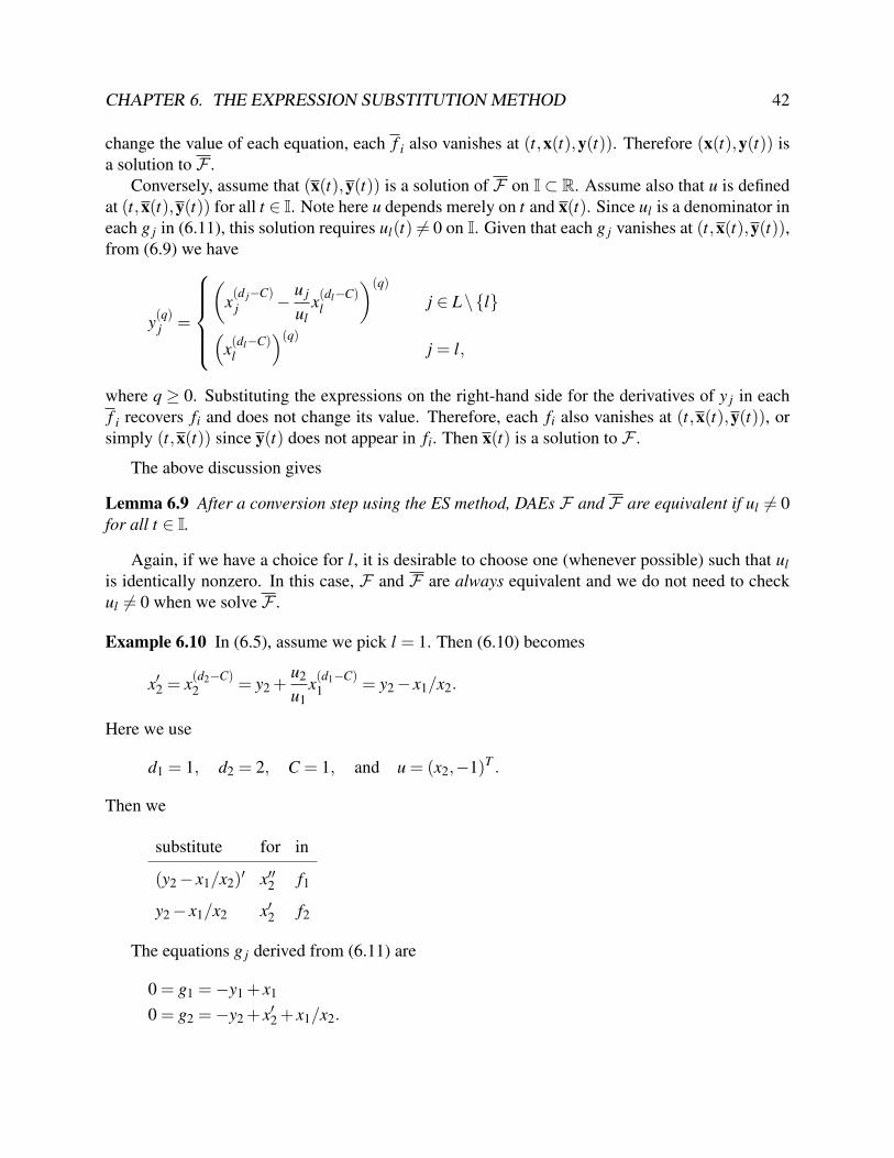
CHAPTER 6. THE EXPRESSION SUBSTITUTION METHOD 43
As l = 1, we can remove g1 and y1, append equation g = g2, and obtain the resulting DAE
0 = f 1 = x1 + e−x′1−x2·(y2−x1/x2)′+g1(t)
= x1 + e−x′1−x2y′2−x′2x1/x2+x′1 +g1(t)
= x1 + e−x2y′2−x′2x1/x2 +g1(t)
0 = f 2 = x1 + x2(y2− x1/x2)+ x22 +g2(t)
= x2y2 + x22 +g2(t)
0 = g =−y2 + x′2 + x1/x2.
Σ =
x1 x2 y2 ci
f 1 0 1 1• 0
f 2 − 0• 0 1
g 0• 1 0 0
d j 0 1 1 Val(Σ) = 1
J =
x1 x2 y2
f 1 1− x′2β/x2 −x1β/x2 −x2β
f 2 0 2x2 + y2 x2
g 1/x2 1 0
det(J) =−x2 +β (2x2 + y2 + x′2− x1/x2)
In J, β = exp(−x2y′2−x′2x1/x2). If det(J) 6= 0, then SA succeeds and gives structural index νS = 2.Here Val(Σ) = 1 < 2 = Val(Σ).
However, the original DAE and the resulting one are equivalent only if u1 = x2 6= 0 on sometime interval I. In practice, it is more desirable to choose l = 2 since ul =−1 is identically nonzero;see also Example 6.3.
Chapter 7
Examples
In this chapter, we illustrate how to apply the LC method and the ES method to several structurallysingular DAEs. When a conversion method succeeds, we obtain an equivalent structurally regularDAE with a nonsingular system Jacobian.
In §7.1, we apply both conversion methods to the 4× 4 linear constant coefficient (coupled)DAE (4.10). The LC method succeeds in converting this problem to a structurally regular DAEin two iterations, reducing the value of the the signature matrix by 2. In contrast, the ES methodreduces the value of the signature matrix by 1 in the first iteration. In the second iteration, thecondition for applying the ES method is not satisfied, and hence it cannot be applied further.
In §7.2, we illustrate both methods on an artificially complicated problem MODPENDB derivedfrom the simple pendulum DAE PEND (3.8). We show in §7.2.1 how the ES method succeeds inconverting this problem to a structurally regular DAE, which has a relatively simple structure. In§7.2.2, the LC method is applied, but yields a considerably more complicated result.
In §7.3, we address Remark 6.2 in more detail: the condition for applying the LC method isnot satisfied for (6.5). If we perform a conversion step, then the value of the signature matrix is notguaranteed to decrease.
7.1 A simple coupled DAERecall the 4×4 linear constant coefficient (coupled) DAE (4.10):
F0 :
0 = f1 =−x′1 + x3 +b1(t)0 = f2 =−x′2 + x4 +b2(t)0 = f3 = x2 + x3 + x4 + c1(t)0 = f4 =−x1 + x3 + x4 + c2(t).
(7.1)
44
CHAPTER 7. EXAMPLES 45
Σ0 =
x1 x2 x3 x4 ci
f1 1• − 0 − 0
f2 − 1• − 0 0
f3 − 0 0• 0 0
f4 0 − 0 0• 0
d j 1 1 0 0 Val(Σ0) = 2
J0 =
x1 x2 x3 x4
f1 −1 0 1 0
f2 0 −1 0 1
f3 0 0 1 1
f4 0 0 1 1
det(J0) = 0
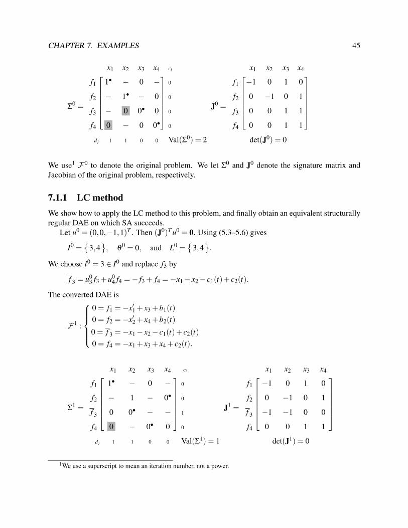
We use1 F0 to denote the original problem. We let Σ0 and J0 denote the signature matrix andJacobian of the original problem, respectively.
7.1.1 LC methodWe show how to apply the LC method to this problem, and finally obtain an equivalent structurallyregular DAE on which SA succeeds.
Let u0 = (0,0,−1,1)T . Then (J0)T u0 = 0. Using (5.3–5.6) gives
I0 ={
3,4}, θ
0 = 0, and L0 ={
3,4}.
We choose l0 = 3 ∈ I0 and replace f3 by
f 3 = u03 f3 +u0
4 f4 =− f3 + f4 =−x1− x2− c1(t)+ c2(t).
The converted DAE is
F1 :
0 = f1 =−x′1 + x3 +b1(t)0 = f2 =−x′2 + x4 +b2(t)
0 = f 3 =−x1− x2− c1(t)+ c2(t)0 = f4 =−x1 + x3 + x4 + c2(t).
Σ1 =
x1 x2 x3 x4 ci
f1 1• − 0 − 0
f2 − 1 − 0• 0
f 3 0 0• − − 1
f4 0 − 0• 0 0
d j 1 1 0 0 Val(Σ1) = 1
J1 =
x1 x2 x3 x4
f1 −1 0 1 0
f2 0 −1 0 1
f 3 −1 −1 0 0
f4 0 0 1 1
det(J1) = 0
1We use a superscript to mean an iteration number, not a power.
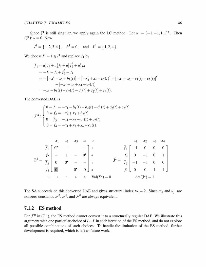
CHAPTER 7. EXAMPLES 46
Since J1 is still singular, we apply again the LC method. Let u1 = (−1,−1,1,1)T . Then(J1)T u = 0. Now
I1 ={
1,2,3,4}, θ
1 = 0, and L1 ={
1,2,4}.
We choose l1 = 1 ∈ I1 and replace f1 by
f 1 = u11 f1 +u1
2 f2 +u13 f ′3 +u1
4 f4
=− f1− f2 + f ′3 + f4
=−[−x′1 + x3 +b1(t)
]−[−x′2 + x4 +b2(t)
]+[−x1− x2− c1(t)+ c2(t)]
′
+[−x1 + x3 + x4 + c2(t)]=−x1−b1(t)−b2(t)− c′1(t)+ c′2(t)+ c2(t).
The converted DAE is
F2 :
0 = f 1 =−x1−b1(t)−b2(t)− c′1(t)+ c′2(t)+ c2(t)0 = f2 =−x′2 + x4 +b2(t)
0 = f 3 =−x1− x2− c1(t)+ c2(t)0 = f4 =−x1 + x3 + x4 + c2(t).
Σ2 =
x1 x2 x3 x4 ci
f 1 0• − − − 1
f2 − 1 − 0• 0
f 3 0 0• − − 1
f4 0 − 0• 0 0
d j 1 1 0 0 Val(Σ2) = 0
J2 =
x1 x2 x3 x4
f 1 −1 0 0 0
f2 0 −1 0 1
f 3 −1 −1 0 0
f4 0 0 1 1
det(J2) = 1
The SA succeeds on this converted DAE and gives structural index νS = 2. Since u0l0 and u1
l1 arenonzero constants, F2, F1, and F0 are always equivalent.
7.1.2 ES methodFor F0 in (7.1), the ES method cannot convert it to a structurally regular DAE. We illustrate thisargument with one particular choice of l ∈ L in each iteration of the ES method, and do not exploreall possible combinations of such choices. To handle the limitation of the ES method, furtherdevelopment is required, which is left as future work.
CHAPTER 7. EXAMPLES 47
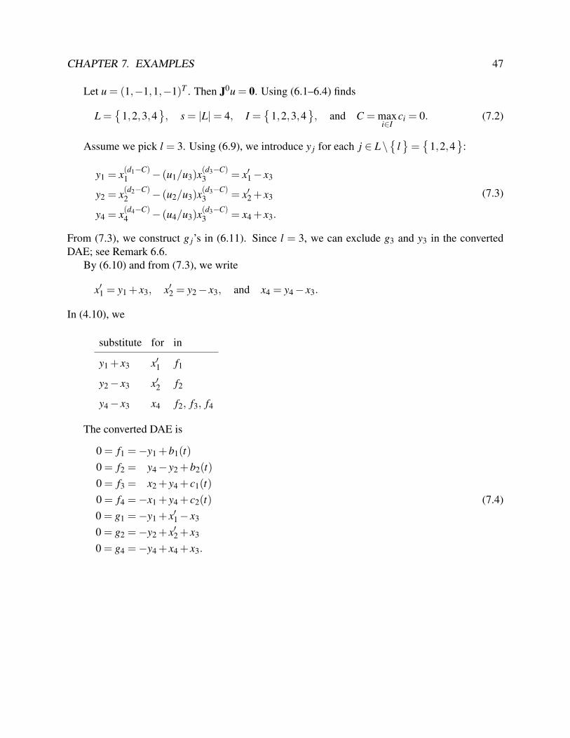
Let u = (1,−1,1,−1)T . Then J0u = 0. Using (6.1–6.4) finds
L ={
1,2,3,4}, s = |L|= 4, I =
{1,2,3,4
}, and C = max
i∈Ici = 0. (7.2)
Assume we pick l = 3. Using (6.9), we introduce y j for each j ∈ L\{
l}={
1,2,4}
:
y1 = x(d1−C)1 − (u1/u3)x
(d3−C)3 = x′1− x3
y2 = x(d2−C)2 − (u2/u3)x
(d3−C)3 = x′2 + x3
y4 = x(d4−C)4 − (u4/u3)x
(d3−C)3 = x4 + x3.
(7.3)
From (7.3), we construct g j’s in (6.11). Since l = 3, we can exclude g3 and y3 in the convertedDAE; see Remark 6.6.
By (6.10) and from (7.3), we write
x′1 = y1 + x3, x′2 = y2− x3, and x4 = y4− x3.
In (4.10), we
substitute for in
y1 + x3 x′1 f1
y2− x3 x′2 f2
y4− x3 x4 f2, f3, f4
The converted DAE is
0 = f1 =−y1 +b1(t)0 = f2 = y4− y2 +b2(t)0 = f3 = x2 + y4 + c1(t)0 = f4 =−x1 + y4 + c2(t)0 = g1 =−y1 + x′1− x3
0 = g2 =−y2 + x′2 + x3
0 = g4 =−y4 + x4 + x3.
(7.4)
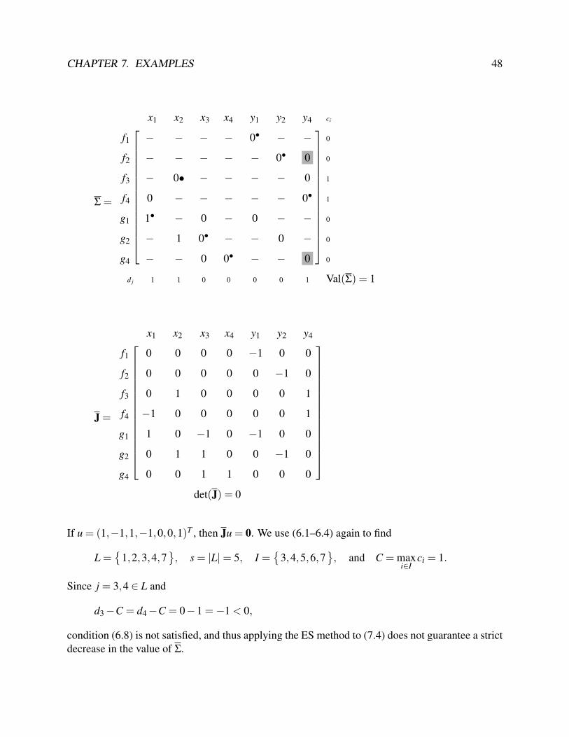
CHAPTER 7. EXAMPLES 48
Σ =
x1 x2 x3 x4 y1 y2 y4 ci
f1 − − − − 0• − − 0
f2 − − − − − 0• 0 0
f3 − 0• − − − − 0 1
f4 0 − − − − − 0• 1
g1 1• − 0 − 0 − − 0
g2 − 1 0• − − 0 − 0
g4 − − 0 0• − − 0 0
d j 1 1 0 0 0 0 1 Val(Σ) = 1
J =
x1 x2 x3 x4 y1 y2 y4
f1 0 0 0 0 −1 0 0
f2 0 0 0 0 0 −1 0
f3 0 1 0 0 0 0 1
f4 −1 0 0 0 0 0 1
g1 1 0 −1 0 −1 0 0
g2 0 1 1 0 0 −1 0
g4 0 0 1 1 0 0 0
det(J) = 0
If u = (1,−1,1,−1,0,0,1)T , then Ju = 0. We use (6.1–6.4) again to find
L ={
1,2,3,4,7}, s = |L|= 5, I =
{3,4,5,6,7
}, and C = max
i∈Ici = 1.
Since j = 3,4 ∈ L and
d3−C = d4−C = 0−1 =−1 < 0,
condition (6.8) is not satisfied, and thus applying the ES method to (7.4) does not guarantee a strictdecrease in the value of Σ.
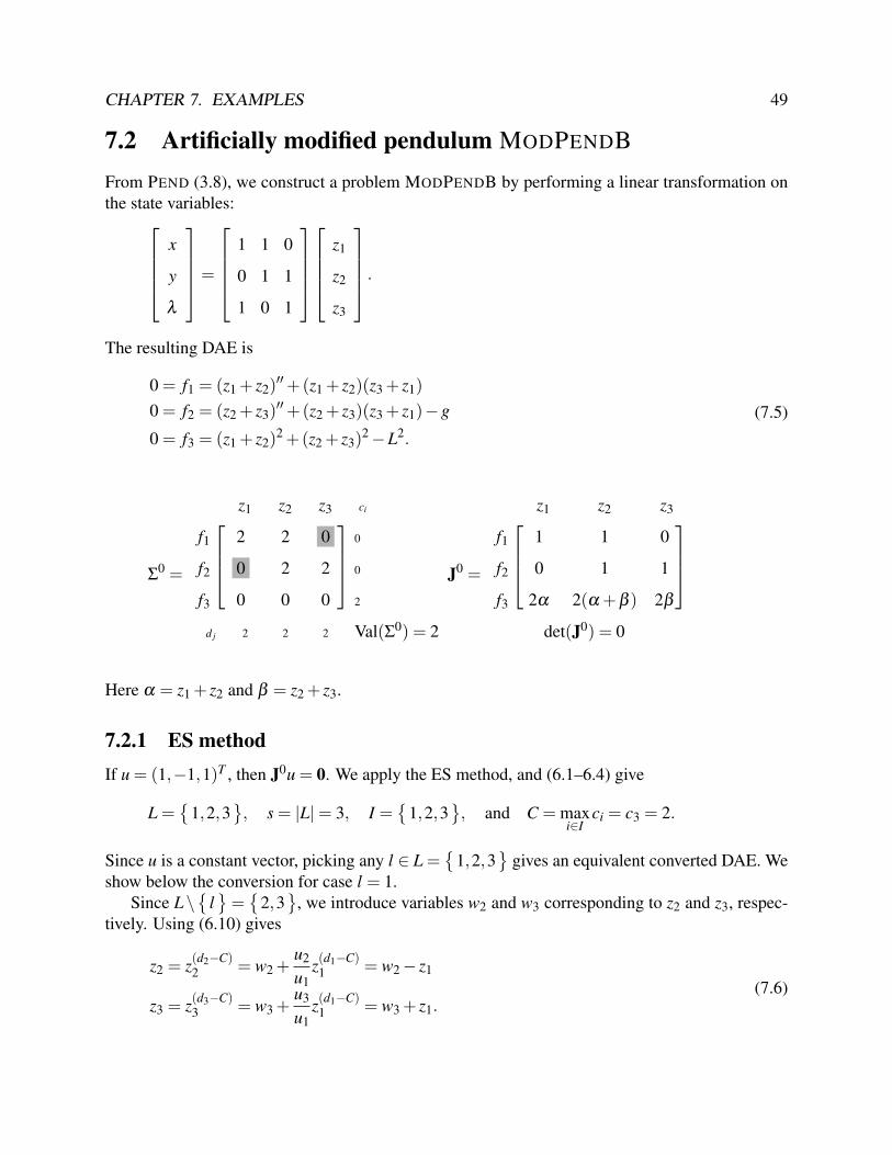
CHAPTER 7. EXAMPLES 49
7.2 Artificially modified pendulum MODPENDB
From PEND (3.8), we construct a problem MODPENDB by performing a linear transformation onthe state variables:
x
y
λ
=
1 1 0
0 1 1
1 0 1
z1
z2
z3
.The resulting DAE is
0 = f1 = (z1 + z2)′′+(z1 + z2)(z3 + z1)
0 = f2 = (z2 + z3)′′+(z2 + z3)(z3 + z1)−g
0 = f3 = (z1 + z2)2 +(z2 + z3)
2−L2.
(7.5)
Σ0 =
z1 z2 z3 ci
f1 2 2 0 0
f2 0 2 2 0
f3 0 0 0 2
d j 2 2 2 Val(Σ0) = 2
J0 =
z1 z2 z3
f1 1 1 0
f2 0 1 1
f3 2α 2(α +β ) 2β
det(J0) = 0
Here α = z1 + z2 and β = z2 + z3.
7.2.1 ES methodIf u = (1,−1,1)T , then J0u = 0. We apply the ES method, and (6.1–6.4) give
L ={
1,2,3}, s = |L|= 3, I =
{1,2,3
}, and C = max
i∈Ici = c3 = 2.
Since u is a constant vector, picking any l ∈ L ={
1,2,3}
gives an equivalent converted DAE. Weshow below the conversion for case l = 1.
Since L\{
l}={
2,3}
, we introduce variables w2 and w3 corresponding to z2 and z3, respec-tively. Using (6.10) gives
z2 = z(d2−C)2 = w2 +
u2
u1z(d1−C)
1 = w2− z1
z3 = z(d3−C)3 = w3 +
u3
u1z(d1−C)
1 = w3 + z1.(7.6)
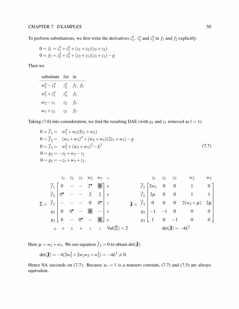
CHAPTER 7. EXAMPLES 50
To perform substitutions, we first write the derivatives z′′1, z′′2 and z′′3 in f1 and f2 explicitly:
0 = f1 = z′′1 + z′′2 +(z1 + z2)(z3 + z1)
0 = f2 = z′′2 + z′′3 +(z2 + z3)(z3 + z1)−g
Then we
substitute for in
w′′2− z′′1 z′′2 f1, f2
w′′3 + z′′1 z′′3 f2
w2− z1 z2 f3
w3 + z1 z3 f3
Taking (7.6) into consideration, we find the resulting DAE (with g1 and y1 removed as l = 1)
0 = f 1 = w′′2 +w2(2z1 +w3)
0 = f 2 = (w2 +w3)′′+(w2 +w3)(2z1 +w3)−g
0 = f 3 = w22 +(w2 +w3)
2−L2
0 = g2 =−z2 +w2− z1
0 = g3 =−z3 +w3 + z1.
(7.7)
Σ =
z1 z2 z3 w2 w3 ci
f 1 0 − − 2• 0 0
f 2 0• − − 2 2 0
f 3 − − − 0 0• 2
g2 0 0• − 0 − 0
g3 0 − 0• − 0 0
d j 0 0 0 2 2 Val(Σ) = 2
J =
z1 z2 z3 w2 w3
f 1 2w2 0 0 1 0
f 2 2µ 0 0 1 1
f 3 0 0 0 2(w2 +µ) 2µ
g2 −1 −1 0 0 0
g3 1 0 −1 0 0
det(J) =−4L2
Here µ = w2 +w3. We use equation f 3 = 0 to obtain det(J):
det(J) =−4(2w22 +2w2w3 +w2
3) =−4L2 6= 0.
Hence SA succeeds on (7.7). Because u1 = 1 is a nonzero constant, (7.7) and (7.5) are alwaysequivalent.
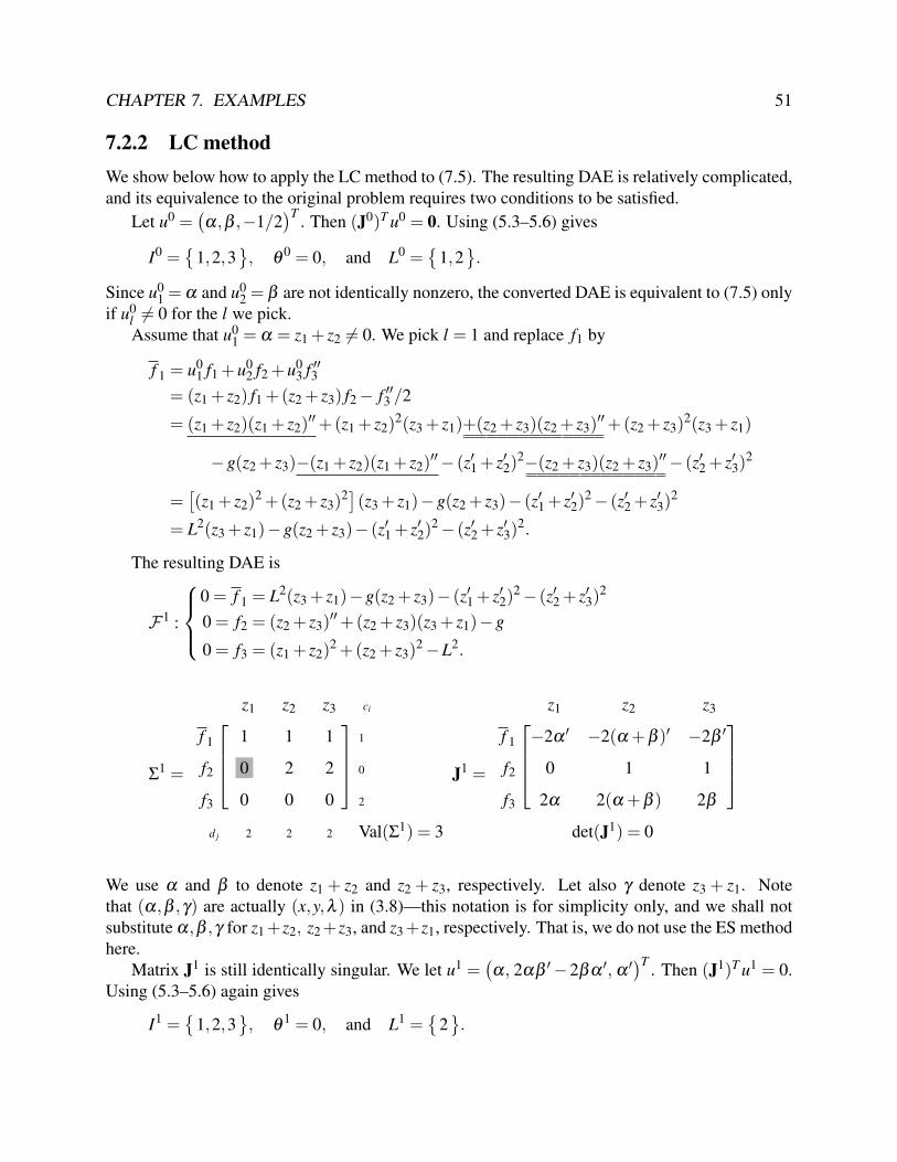
CHAPTER 7. EXAMPLES 51
7.2.2 LC methodWe show below how to apply the LC method to (7.5). The resulting DAE is relatively complicated,and its equivalence to the original problem requires two conditions to be satisfied.
Let u0 =(α,β ,−1/2
)T . Then (J0)T u0 = 0. Using (5.3–5.6) gives
I0 ={
1,2,3}, θ
0 = 0, and L0 ={
1,2}.
Since u01 = α and u0
2 = β are not identically nonzero, the converted DAE is equivalent to (7.5) onlyif u0
l 6= 0 for the l we pick.Assume that u0
1 = α = z1 + z2 6= 0. We pick l = 1 and replace f1 by
f 1 = u01 f1 +u0
2 f2 +u03 f ′′3
= (z1 + z2) f1 +(z2 + z3) f2− f ′′3 /2
= (z1 + z2)(z1 + z2)′′+(z1 + z2)
2(z3 + z1)+(z2 + z3)(z2 + z3)′′+(z2 + z3)
2(z3 + z1)
−g(z2 + z3)−(z1 + z2)(z1 + z2)′′− (z′1 + z′2)
2−(z2 + z3)(z2 + z3)′′− (z′2 + z′3)
2
=[(z1 + z2)
2 +(z2 + z3)2](z3 + z1)−g(z2 + z3)− (z′1 + z′2)
2− (z′2 + z′3)2
= L2(z3 + z1)−g(z2 + z3)− (z′1 + z′2)2− (z′2 + z′3)
2.
The resulting DAE is
F1 :
0 = f 1 = L2(z3 + z1)−g(z2 + z3)− (z′1 + z′2)
2− (z′2 + z′3)2
0 = f2 = (z2 + z3)′′+(z2 + z3)(z3 + z1)−g
0 = f3 = (z1 + z2)2 +(z2 + z3)
2−L2.
Σ1 =
z1 z2 z3 ci
f 1 1 1 1 1
f2 0 2 2 0
f3 0 0 0 2
d j 2 2 2 Val(Σ1) = 3
J1 =
z1 z2 z3
f 1 −2α ′ −2(α +β )′ −2β ′
f2 0 1 1
f3 2α 2(α +β ) 2β
det(J1) = 0
We use α and β to denote z1 + z2 and z2 + z3, respectively. Let also γ denote z3 + z1. Notethat (α,β ,γ) are actually (x,y,λ ) in (3.8)—this notation is for simplicity only, and we shall notsubstitute α,β ,γ for z1+z2, z2+z3, and z3+z1, respectively. That is, we do not use the ES methodhere.
Matrix J1 is still identically singular. We let u1 =(α, 2αβ ′−2βα ′, α ′
)T . Then (J1)T u1 = 0.Using (5.3–5.6) again gives
I1 ={
1,2,3}, θ
1 = 0, and L1 ={
2}.
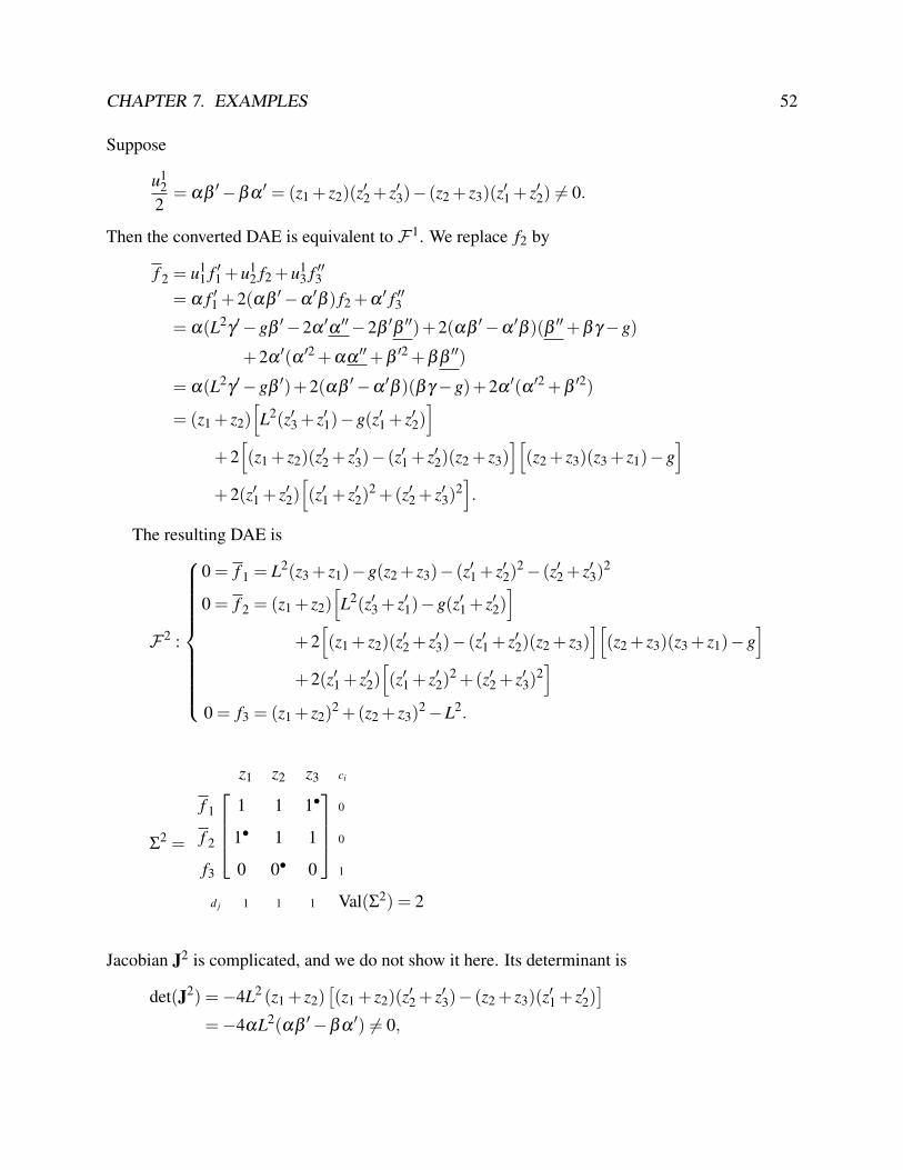
CHAPTER 7. EXAMPLES 52
Suppose
u12
2= αβ
′−βα′ = (z1 + z2)(z′2 + z′3)− (z2 + z3)(z′1 + z′2) 6= 0.
Then the converted DAE is equivalent to F1. We replace f2 by
f 2 = u11 f ′1 +u1
2 f2 +u13 f ′′3
= α f ′1 +2(αβ′−α
′β ) f2 +α
′ f ′′3= α(L2
γ′−gβ
′−2α′α′′−2β
′β′′)+2(αβ
′−α′β )(β ′′+βγ−g)
+2α′(α ′2 +αα
′′+β′2 +ββ
′′)
= α(L2γ′−gβ
′)+2(αβ′−α
′β )(βγ−g)+2α
′(α ′2 +β′2)
= (z1 + z2)[L2(z′3 + z′1)−g(z′1 + z′2)
]+2[(z1 + z2)(z′2 + z′3)− (z′1 + z′2)(z2 + z3)
][(z2 + z3)(z3 + z1)−g
]+2(z′1 + z′2)
[(z′1 + z′2)
2 +(z′2 + z′3)2].
The resulting DAE is
F2 :
0 = f 1 = L2(z3 + z1)−g(z2 + z3)− (z′1 + z′2)2− (z′2 + z′3)
2
0 = f 2 = (z1 + z2)[L2(z′3 + z′1)−g(z′1 + z′2)
]+2[(z1 + z2)(z′2 + z′3)− (z′1 + z′2)(z2 + z3)
][(z2 + z3)(z3 + z1)−g
]+2(z′1 + z′2)
[(z′1 + z′2)
2 +(z′2 + z′3)2]
0 = f3 = (z1 + z2)2 +(z2 + z3)
2−L2.
Σ2 =
z1 z2 z3 ci
f 1 1 1 1• 0
f 2 1• 1 1 0
f3 0 0• 0 1
d j 1 1 1 Val(Σ2) = 2
Jacobian J2 is complicated, and we do not show it here. Its determinant is
det(J2) =−4L2 (z1 + z2)[(z1 + z2)(z′2 + z′3)− (z2 + z3)(z′1 + z′2)
]=−4αL2(αβ
′−βα′) 6= 0,
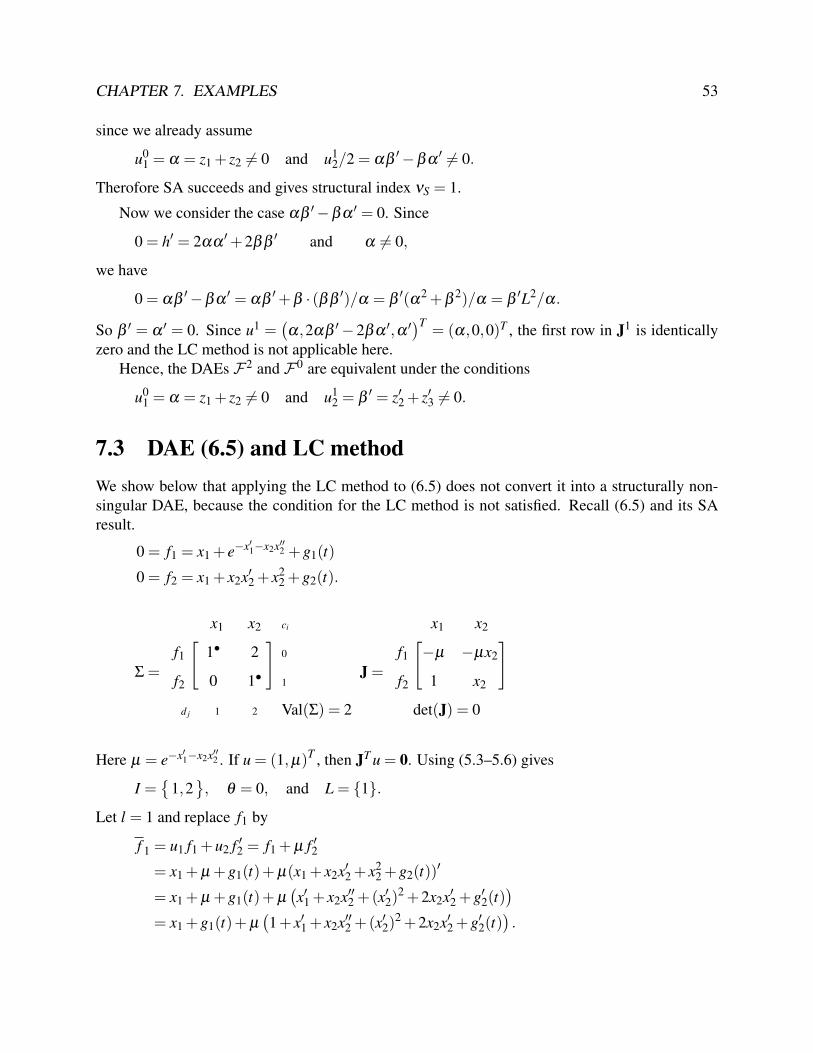
CHAPTER 7. EXAMPLES 53
since we already assume
u01 = α = z1 + z2 6= 0 and u1
2/2 = αβ′−βα
′ 6= 0.
Therofore SA succeeds and gives structural index νS = 1.
Now we consider the case αβ ′−βα ′ = 0. Since
0 = h′ = 2αα′+2ββ
′ and α 6= 0,
we have
0 = αβ′−βα
′ = αβ′+β · (ββ
′)/α = β′(α2 +β
2)/α = β′L2/α.
So β ′ = α ′ = 0. Since u1 =(α,2αβ ′− 2βα ′,α ′
)T= (α,0,0)T , the first row in J1 is identically
zero and the LC method is not applicable here.Hence, the DAEs F2 and F0 are equivalent under the conditions
u01 = α = z1 + z2 6= 0 and u1
2 = β′ = z′2 + z′3 6= 0.
7.3 DAE (6.5) and LC methodWe show below that applying the LC method to (6.5) does not convert it into a structurally non-singular DAE, because the condition for the LC method is not satisfied. Recall (6.5) and its SAresult.
0 = f1 = x1 + e−x′1−x2x′′2 +g1(t)
0 = f2 = x1 + x2x′2 + x22 +g2(t).
Σ =
x1 x2 ci[ ]f1 1• 2 0
f2 0 1• 1
d j 1 2 Val(Σ) = 2
J =
x1 x2[ ]f1 −µ −µx2
f2 1 x2
det(J) = 0
Here µ = e−x′1−x2x′′2 . If u = (1,µ)T , then JT u = 0. Using (5.3–5.6) gives
I ={
1,2}, θ = 0, and L = {1}.
Let l = 1 and replace f1 by
f 1 = u1 f1 +u2 f ′2 = f1 +µ f ′2= x1 +µ +g1(t)+µ(x1 + x2x′2 + x2
2 +g2(t))′
= x1 +µ +g1(t)+µ(x′1 + x2x′′2 +(x′2)
2 +2x2x′2 +g′2(t))
= x1 +g1(t)+µ(1+ x′1 + x2x′′2 +(x′2)
2 +2x2x′2 +g′2(t)).
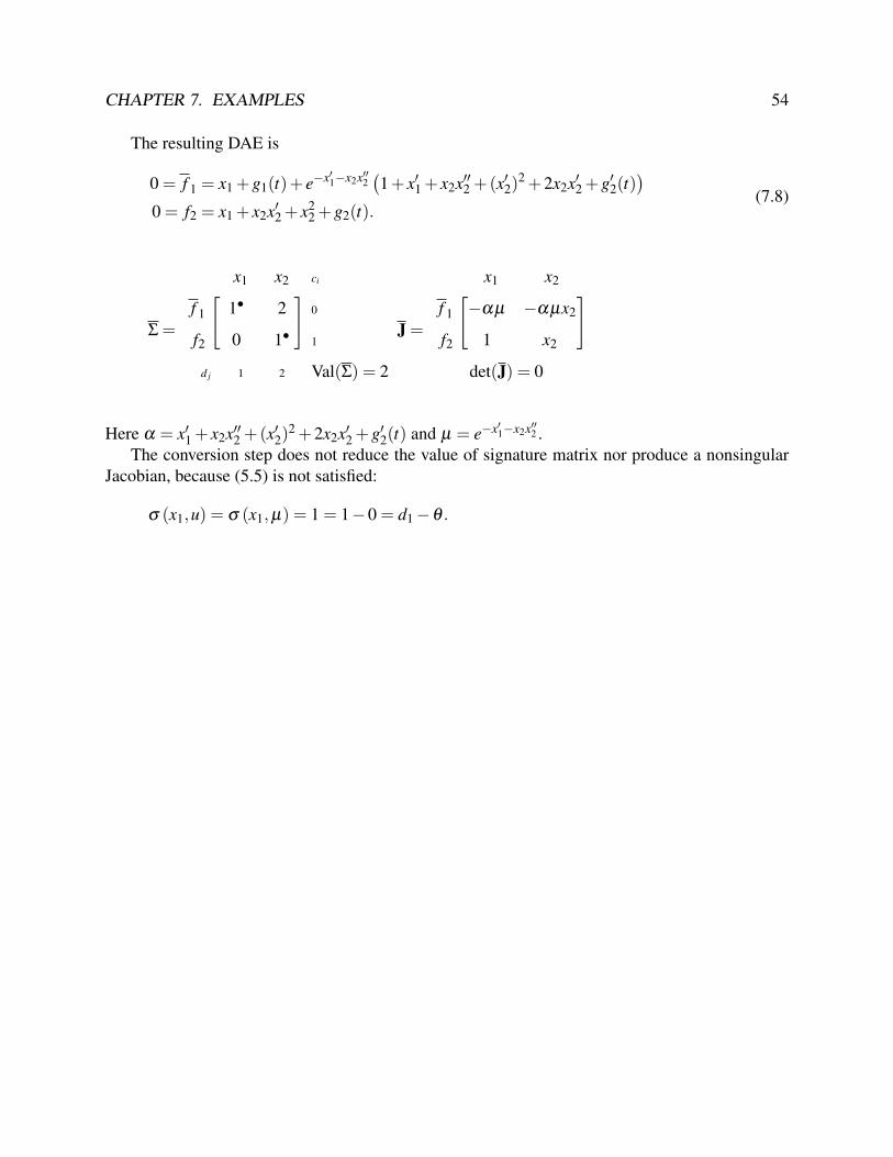
CHAPTER 7. EXAMPLES 54
The resulting DAE is
0 = f 1 = x1 +g1(t)+ e−x′1−x2x′′2(1+ x′1 + x2x′′2 +(x′2)
2 +2x2x′2 +g′2(t))
0 = f2 = x1 + x2x′2 + x22 +g2(t).
(7.8)
Σ =
x1 x2 ci[ ]f 1 1• 2 0
f2 0 1• 1
d j 1 2 Val(Σ) = 2
J =
x1 x2[ ]f 1 −αµ −αµx2
f2 1 x2
det(J) = 0
Here α = x′1 + x2x′′2 +(x′2)2 +2x2x′2 +g′2(t) and µ = e−x′1−x2x′′2 .
The conversion step does not reduce the value of signature matrix nor produce a nonsingularJacobian, because (5.5) is not satisfied:
σ (x1,u) = σ (x1,µ) = 1 = 1−0 = d1−θ .

Chapter 8
Conclusion and future work
We identified two types of structural analysis’s failure. For the first type, the system Jacobian isstructurally singular, and the failure is likely due to hidden symbolic cancellations. One way tohandle this is to perform symbolic simplifications before applying SA.
We focused on dealing with the second type, where SA fails in a less obvious way. In this case,the Jacobian is not structurally singular but is still identically singular. We proposed two symbolic-numeric methods for converting a DAE with such singular Jacobian to an equivalent DAE on whichSA succeeds with nonsingular Jacobian, provided some conditions are satisfied. Such conditionscan be checked automatically. These conversion methods provably succeed and thus allow SA tohandle more DAE types. Our methods enable SA to better recognize the true structure of a DAE,and thus SA is more likely to succeed and obtain correct structural information. Moreover, ourmethods provide insights into reasons for SA’s failures, which were not well understood before.
We summarize the two conversion methods here. The LC method is more straightforward: itkeeps the size of the system and replaces only one equation within a conversion step. The ESmethod requires more conditions to apply. It augments the system and changes several equationswithin a conversion step, which generally takes more symbolic operations. The common goal ofboth methods is to reduce the value of the signature matrix; this value is also the number of degreesof freedom reported by the SA. We also need to ensure that the converted DAE is equivalent tothe original one: on some time interval, a solution of the original DAE should be a solution to theconverted DAE, and vice versa. Moreover, it is desirable to choose a conversion (if possible) suchthat we do not need to monitor the equivalence condition (ul 6= 0) when we solve the convertedproblem.
A practical question worth considering is how to choose the appropriate conversion methodbetween the two for a given structurally singular DAE. For many of the examples we have stud-ied, it is fairly common that conditions of only one method are satisfied; see §7.1 and §7.3. Forsome other DAEs, provided conditions of both methods are satisfied, applying one method usuallyrequires fewer symbolic manipulations than applying the other; see MODPENDB in §7.2. In thelatter case, we examine if a conversion has an identically nonzero ul , such that the converted DAEand the original one are always equivalent. If applying either method guarantees such equivalence,we prefer the LC method because it changes only one equation and maintains the problem size.
55
CHAPTER 8. CONCLUSION AND FUTURE WORK 56
Our next goal is to combine these conversion methods with block triangular forms (BTFs) ofa DAE [28, 29]. If the Jacobian is identically singular and the DAE has a non-trivial BTF, that is,it has two or more diagonal blocks, then we can locate the block that leads to the singularity, andperform a conversion step on this singular block. Using this approach, we have already made someprogress and managed to convert several problems, including the Campbell-Griepentrog RobotArm and the Ring Modulator, into SA success cases. However, more careful studies are requiredand details need to be worked out.
Future work also includes rigorous implementation of these conversion methods in MATLAB.We currently have a prototype code, which builds upon our structural analyzer package DAESA [23]and takes advantage of MATLAB’s symbolic toolbox. We can call DAESA functions to display aconverted DAE’s structure, perform quasilinearity analysis, and print out a solution scheme [24].Our goal is to eventually build a complete tool for performing DAE conversions.
Another interesting direction for research is combining the dummy derivative index reductionmethod [17] with the conversion techniques. McKenzie et al. [19] show that dummy derivativemethod and the Σ-method share some similarities. The former method converts a high-index DAEinto a low-index one by introducing dummy algebraic variables and augmenting the system. Sup-pose we adopt this methodology. When a condition for applying a conversion method is violated,applying some dummy-derivative-like strategy may help make a conversion possible.
Our conversion methods require a symbolic toolbox that is capable of performing nontrivialsymbolic arithmetic operations, differentiation, and simplifications. However, we only focus on alinear combination of the equations (in the LC method) and a linear combination of derivatives ofhighest order (in the ES method). How to further exploit symbolic tools to develop other conversionmethods should deserve some investigation.
We conclude with a conjecture here. In all our experiments, when we transform a DAE withidentically singular Jacobian to an equivalent solvable DAE with generically nonsingular Jacobian,the value of the signature matrix always decreases. As Pryce points out in [26], the solvability ofa DAE lies within its inherent nature, not the way it is formulated nor the method that analyzesit. We conjecture that, if a reformulation of a structurally singular DAE results in an equivalentsolvable DAE, then the value of the signature matrix always decreases. However, based on ourcurrent knowledge, it seems difficult to prove this conjecture.
Appendix A
Proofs for the ES method
For readers’ convenience, we recall the notation from Sections 6.1 and 6.2:
L ={
j | u j 6= 0}= {1 : s}, s = |L|,
I ={
i | d j− ci = σi j for some j ∈ L}, C = max
i∈Ici.
We also assume the conditions for applying the ES method are satisfied:
σ(x j,u
)≤{
d j−C−1 if j ∈ Ld j−C otherwise, (A.1)
and
d j−C ≥ 0 for all j ∈ L.
Denote
I = {1 : n}\ I ={
i | d j− ci > σi j for all j ∈ L}, and
L = {1 : n}\L ={
j | u j = 0}= {s+1 : n}.
In the following, we assume we pick a column index l ∈ L in a conversion step using the ESmethod. We also assume ul 6= 0 for all t in some I⊂ R.
A.1 Preliminary results for the proof of Lemma 6.4Lemma A.1 Let l ∈ L. If (A.1) holds, then for an r ∈ L\{l},
σ
(x j,yr +
ur
ulx(dl−C)
l
)≤
{d j−C−1 if j ∈ L\{l}=
{1, . . . , l−1, l +1, . . . ,s
}d j−C if j ∈ L∪{l}=
{l,s+1,s+2, . . . ,n
}.
(A.2)
57
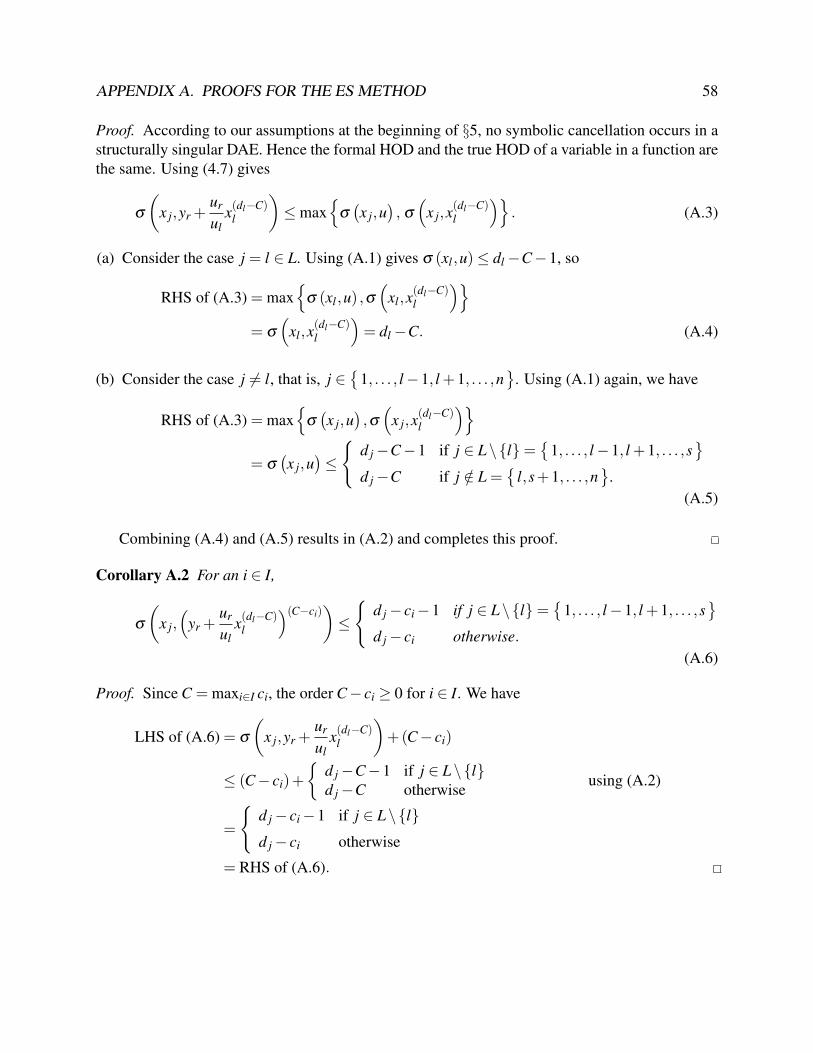
APPENDIX A. PROOFS FOR THE ES METHOD 58
Proof. According to our assumptions at the beginning of §5, no symbolic cancellation occurs in astructurally singular DAE. Hence the formal HOD and the true HOD of a variable in a function arethe same. Using (4.7) gives
σ
(x j,yr +
ur
ulx(dl−C)
l
)≤max
{σ(x j,u
), σ
(x j,x
(dl−C)l
)}. (A.3)
(a) Consider the case j = l ∈ L. Using (A.1) gives σ (xl,u)≤ dl−C−1, so
RHS of (A.3) = max{
σ (xl,u) ,σ(
xl,x(dl−C)l
)}= σ
(xl,x
(dl−C)l
)= dl−C. (A.4)
(b) Consider the case j 6= l, that is, j ∈{
1, . . . , l−1, l +1, . . . ,n}
. Using (A.1) again, we have
RHS of (A.3) = max{
σ(x j,u
),σ(
x j,x(dl−C)l
)}= σ
(x j,u
)≤
{d j−C−1 if j ∈ L\{l}=
{1, . . . , l−1, l +1, . . . ,s
}d j−C if j /∈ L =
{l,s+1, . . . ,n
}.
(A.5)
Combining (A.4) and (A.5) results in (A.2) and completes this proof.
Corollary A.2 For an i ∈ I,
σ
(x j,(
yr +ur
ulx(dl−C)
l
)(C−ci))≤
{d j− ci−1 if j ∈ L\{l}=
{1, . . . , l−1, l +1, . . . ,s
}d j− ci otherwise.
(A.6)
Proof. Since C = maxi∈I ci, the order C− ci ≥ 0 for i ∈ I. We have
LHS of (A.6) = σ
(x j,yr +
ur
ulx(dl−C)
l
)+(C− ci)
≤ (C− ci)+
{d j−C−1 if j ∈ L\{l}d j−C otherwise using (A.2)
=
{d j− ci−1 if j ∈ L\{l}d j− ci otherwise
= RHS of (A.6).
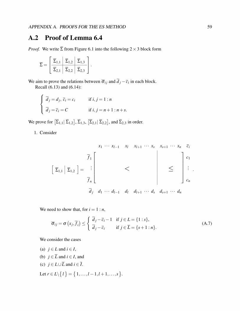
APPENDIX A. PROOFS FOR THE ES METHOD 59
A.2 Proof of Lemma 6.4Proof. We write Σ from Figure 6.1 into the following 2×3 block form
Σ =
Σ1,1 Σ1,2 Σ1,3
Σ2,1 Σ2,2 Σ2,3
.We aim to prove the relations between σ i j and d j− ci in each block.
Recall (6.13) and (6.14):d j = d j, ci = ci if i, j = 1 : n
d j = ci =C if i, j = n+1 : n+ s.
We prove for[Σ1,1| Σ1,2
], Σ1,3,
[Σ2,1| Σ2,2
], and Σ2,3 in order.
1. Consider
[Σ1,1 Σ1,2
]=
x1 · · · xl−1 xl xl+1 · · · xs xs+1 · · · xn ci
f 1 c1
... < ≤ ...
f n cn
d j d1 · · · dl−1 dl dl+1 · · · ds ds+1 · · · dn
.
We need to show that, for i = 1 : n,
σ i j = σ(x j, f i
)≤
{d j− ci−1 if j ∈ L = {1 : s},d j− ci if j ∈ L = {s+1 : n}.
(A.7)
We consider the cases
(a) j ∈ L and i ∈ I,
(b) j ∈ L and i ∈ I, and
(c) j ∈ L∪L and i ∈ I.
Let r ∈ L\{
l}={
1, . . . , l−1, l +1, . . . ,s}
.

APPENDIX A. PROOFS FOR THE ES METHOD 60
(a) Consider j ∈ L\{l}. By Corollary A.2, the HOD of x j is ≤ d j− ci−1 in every(yr +
ur
ulx(dl−C)
l
)(C−ci)
that replaces x(dr−ci)r in an fi—here r ∈ L\
{l}
, which includes j. Therefore,
σ(x j, f i
)≤ d j− ci−1 for j ∈ L\
{l}, i ∈ I. (A.8)
Now consider j = l ∈ L. We show below that ∂ f i/∂x(dl−ci)l = 0, which implies x(dl−ci)
ldoes not appear in f i, i ∈ I. That is,
σ(xl, f i
)≤ dl− ci−1 for i ∈ I. (A.9)
Using (A.1) gives
σ
(xl,
ur
ul
)≤ σ (xl,u)≤ dl−C−1.
Also
σ
(xl,yr +
ur
ulx(dl−C)
l
)= max
{σ (xl,u) ,σ
(xl,x
(dl−C)l
)}= dl−C.
Since C− ci ≥ 0 for i ∈ I, we apply Griewank’s lemma (5.1), with q =C− ci, to
x(dr−C)r = yr +
ur
ulx(dl−C)
l (A.10)
from (6.10). Differentiating both sides of (A.10) with respect to x(dl−C)l gives
ur
ul=
∂x(dr−C)r
∂x(dl−C)l
=∂x(dr−C+C−ci)
r
∂x(dl−C+C−ci)l
=∂x(dr−ci)
r
∂x(dl−ci)l
. (A.11)
Then
∂ f i
∂x(dl−ci)l
=∂ fi
∂x(dl−ci)l
+ ∑r∈L\{l}
∂ fi
∂x(dr−ci)r
· ∂x(dr−ci)r
∂x(dl−ci)l
by the chain rule
= Jil + ∑r∈L\{l}
Jir ·ur
ulby (A.11)
=1ul
∑r∈L
Jirur =1ul(Ju)i = 0 because Ju = 0.
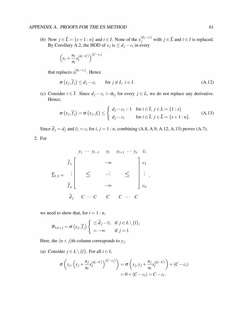
APPENDIX A. PROOFS FOR THE ES METHOD 61
(b) Now j ∈ L = {s+1 : n} and i ∈ I. None of the x(d j−ci)j with j ∈ L and i ∈ I is replaced.
By Corollary A.2, the HOD of x j is ≤ d j− ci in every(yr +
ur
ulx(dl−C)
l
)(C−ci)
that replaces x(dr−ci)r . Hence
σ(x j, f i
)≤ d j− ci for j /∈ L, i ∈ I. (A.12)
(c) Consider i ∈ I. Since d j− ci > σi j for every j ∈ L, we do not replace any derivative.Hence,
σ(x j, f i
)= σ
(x j, fi
)≤
{d j− ci−1 for i ∈ I, j ∈ L = {1 : s}d j− ci for i ∈ I, j ∈ L = {s+1 : n}.
(A.13)
Since d j = d j and ci = ci for i, j = 1 : n, combining (A.8, A.9, A.12, A.13) proves (A.7).
2. For
Σ1,3 =
y1 · · · yl−1 yl yl+1 · · · ys ci
f 1 −∞ c1
... ≤ −... ≤ ...
f n −∞ cn
d j C · · · C C C · · · C
,
we need to show that, for i = 1 : n,
σ i,n+ j = σ(y j, f i
){ ≤ d j− ci if j ∈ L\{l},=−∞ if j = l.
Here, the (n+ j)th column corresponds to y j.
(a) Consider j ∈ L\{l}. For all i ∈ I,
σ
(y j,(
y j +u j
ulx(dl−C)
l
)(C−ci))= σ
(y j,y j +
u j
ulx(dl−C)
l
)+(C− ci)
= 0+(C− ci) =C− ci.
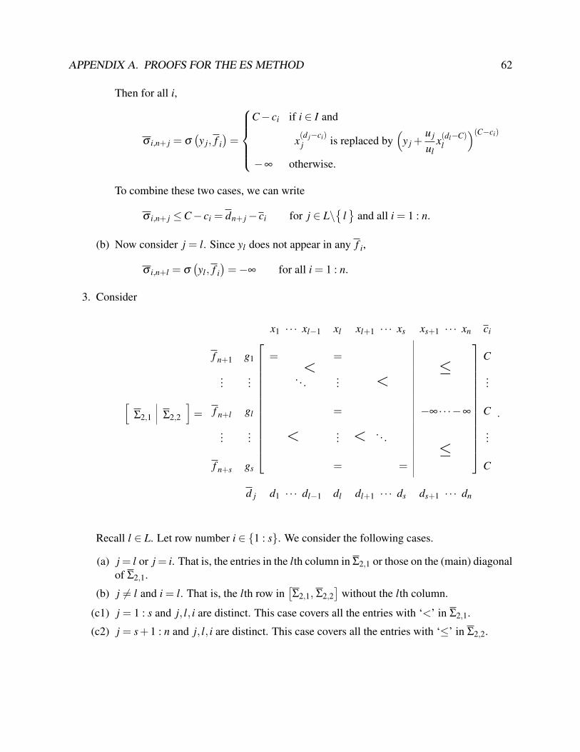
APPENDIX A. PROOFS FOR THE ES METHOD 62
Then for all i,
σ i,n+ j = σ(y j, f i
)=
C− ci if i ∈ I and
x(d j−ci)j is replaced by
(y j +
u j
ulx(dl−C)
l
)(C−ci)
−∞ otherwise.
To combine these two cases, we can write
σ i,n+ j ≤C− ci = dn+ j− ci for j ∈ L\{
l}
and all i = 1 : n.
(b) Now consider j = l. Since yl does not appear in any f i,
σ i,n+l = σ(yl, f i
)=−∞ for all i = 1 : n.
3. Consider
[Σ2,1 Σ2,2
]=
x1 · · · xl−1 xl xl+1 · · · xs xs+1 · · · xn ci
f n+1 g1 =<
=
<≤
C
...... . . . ...
...
f n+l gl = −∞ · · ·−∞ C
...... < ... . . .
≤...
f n+s gs =
<
= C
d j d1 · · · dl−1 dl dl+1 · · · ds ds+1 · · · dn
.
Recall l ∈ L. Let row number i ∈ {1 : s}. We consider the following cases.
(a) j = l or j = i. That is, the entries in the lth column in Σ2,1 or those on the (main) diagonalof Σ2,1.
(b) j 6= l and i = l. That is, the lth row in[Σ2,1, Σ2,2
]without the lth column.
(c1) j = 1 : s and j, l, i are distinct. This case covers all the entries with ‘<’ in Σ2,1.
(c2) j = s+1 : n and j, l, i are distinct. This case covers all the entries with ‘≤’ in Σ2,2.
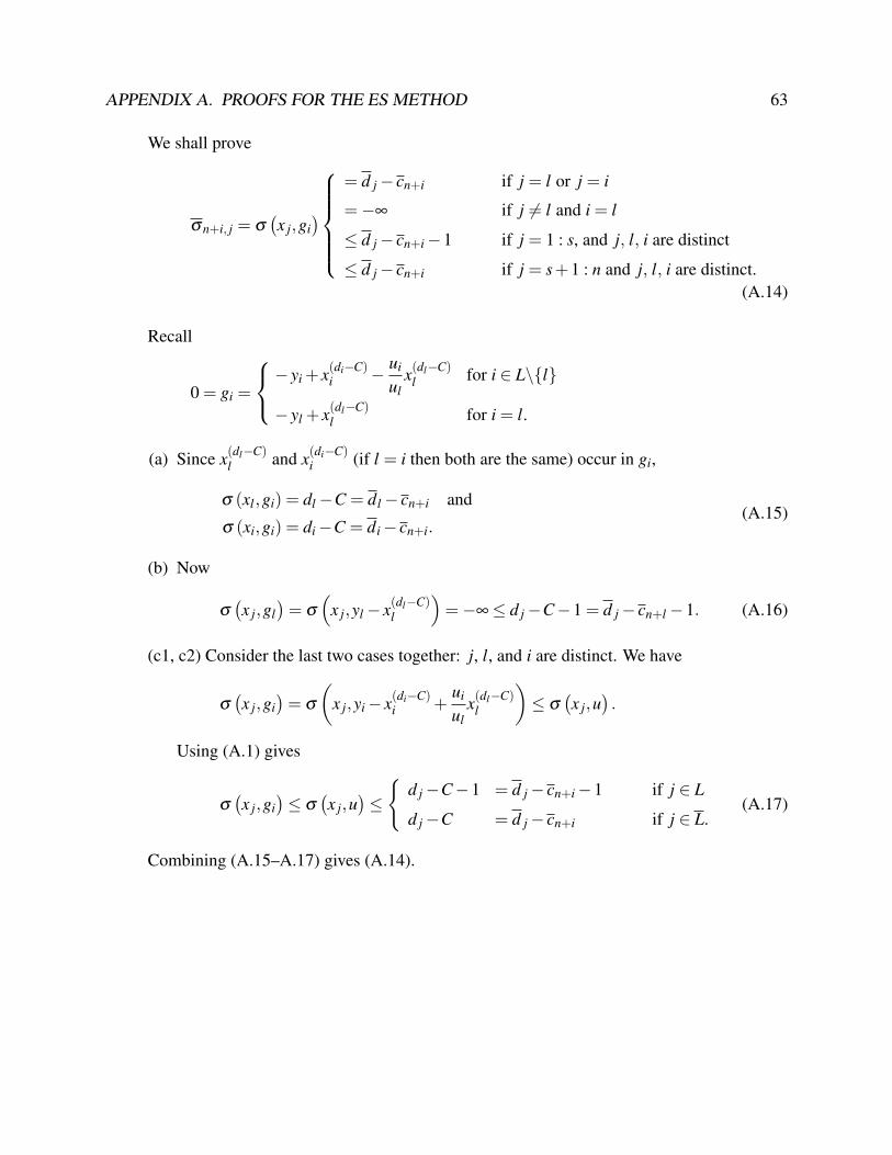
APPENDIX A. PROOFS FOR THE ES METHOD 63
We shall prove
σn+i, j = σ(x j,gi
)
= d j− cn+i if j = l or j = i
=−∞ if j 6= l and i = l
≤ d j− cn+i−1 if j = 1 : s, and j, l, i are distinct
≤ d j− cn+i if j = s+1 : n and j, l, i are distinct.(A.14)
Recall
0 = gi =
− yi + x(di−C)i − ui
ulx(dl−C)
l for i ∈ L\{l}
− yl + x(dl−C)l for i = l.
(a) Since x(dl−C)l and x(di−C)
i (if l = i then both are the same) occur in gi,
σ (xl,gi) = dl−C = dl− cn+i and
σ (xi,gi) = di−C = di− cn+i.(A.15)
(b) Now
σ(x j,gl
)= σ
(x j,yl− x(dl−C)
l
)=−∞≤ d j−C−1 = d j− cn+l−1. (A.16)
(c1, c2) Consider the last two cases together: j, l, and i are distinct. We have
σ(x j,gi
)= σ
(x j,yi− x(di−C)
i +ui
ulx(dl−C)
l
)≤ σ
(x j,u
).
Using (A.1) gives
σ(x j,gi
)≤ σ
(x j,u
)≤
{d j−C−1 = d j− cn+i−1 if j ∈ L
d j−C = d j− cn+i if j ∈ L.(A.17)
Combining (A.15–A.17) gives (A.14).
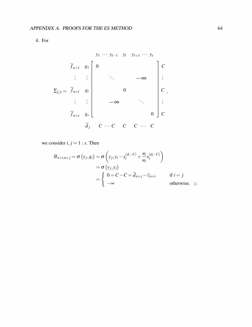
APPENDIX A. PROOFS FOR THE ES METHOD 64
4. For
Σ2,3 =
y1 · · · yl−1 yl yl+1 · · · ys
f n+1 g1 0 C
...... . . . −∞
...
f n+l gl 0 C
...... −∞
. . . ...
f n+s gs 0 C
d j C · · · C C C · · · C
,
we consider i, j = 1 : s. Then
σn+i,n+ j = σ(y j,gi
)= σ
(y j,yi− x(di−C)
i +ui
ulx(dl−C)
l
)= σ
(y j,yi
)=
{0 =C−C = dn+ j− cn+i if i = j
−∞ otherwise.
Appendix B
More examples
We review how to remedy several structurally singular DAEs from the literature. We discuss theindex-5 Campbell-Griepentrog Robot Arm DAE in §B.1, the transistor amplifier DAE in §B.2, andthe ring modulator problem in §B.3. We also show in §B.4 how to “fix” the index overestimationproblem on Reißig’s family of linear DAEs, for which SA produces a nonsingular system Jacobianbut overestimates the index. After we apply a technique similar to the linear combination method,SA reports the correct index νS = 1 on this family of DAEs.
B.1 Robot ArmWe slightly simplify the two-link robot arm problem in [5] by writing the derivatives of x1,x2, andx3 implicitly in the equations:
0 = f1 = x′′1−[2c(x3)(x′1 + x′3)
2 + x′21 d(x3)
+(2x3− x2)(a(x3)+2b(x3)
)+a(x3)(u1−u2)
]0 = f2 = x′′2−
[−2c(x3)(x′1 + x′3)
2− x′21 d(x3)
+(2x3− x2)(1−3a(x3)−2b(x3)
)−a(x3)u1 +
(a(x3)+1
)u2
]0 = f3 = x′′3−
[−2c(x3)(x′1 + x′3)
2− x′21 d(x3)+(2x3− x2)(a(x3)−9b(x3)
)−2x′21 c(x3)−d(x3)
(x′1 + x′3
)2−(a(x3)+b(x3)
)(u1−u2)
]0 = f4 = cosx1 + cos(x1 + x3)− p1(t)0 = f5 = sinx1 + sin(x1 + x3)− p2(t),
(B.1)
65
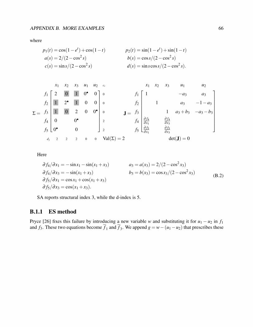
APPENDIX B. MORE EXAMPLES 66
where
p1(t) = cos(1− et)+ cos(1− t) p2(t) = sin(1− et)+ sin(1− t)
a(s) = 2/(2− cos2 s) b(s) = coss/(2− cos2 s)
c(s) = sins/(2− cos2 s) d(s) = sinscoss/(2− cos2 s).
Σ =
x1 x2 x3 u1 u2 ci
f1 2 0 1 0• 0 0
f2 1 2• 1 0 0 0
f3 1 0 2 0 0• 0
f4 0 0• 2
f5 0• 0 2
d j 2 2 2 0 0 Val(Σ) = 2
J =
x1 x2 x3 u1 u2
f1 1 −a3 a3
f2 1 a3 −1−a3
f3 1 a3 +b3 −a3−b3
f4∂ f4∂x1
∂ f4∂x3
f5∂ f5∂x1
∂ f5∂x3
det(J) = 0
Here
∂ f4/∂x1 =−sinx1− sin(x1 + x3) a3 = a(x3) = 2/(2− cos2 x3)
∂ f4/∂x3 =−sin(x1 + x3) b3 = b(x3) = cosx3/(2− cos2 x3)
∂ f5/∂x1 = cosx1 + cos(x1 + x3)
∂ f5/∂x3 = cos(x1 + x3).
(B.2)
SA reports structural index 3, while the d-index is 5.
B.1.1 ES methodPryce [26] fixes this failure by introducing a new variable w and substituting it for u1− u2 in f1and f3. These two equations become f 1 and f 3. We append g = w−(u1−u2) that prescribes these

APPENDIX B. MORE EXAMPLES 67
substitutions and obtain the converted DAE:
0 = f 1 =x′′1−[2c(x3)(x′1 + x′3)
2 + x′21 d(x3)
+(2x3− x2)(a(x3)+2b(x3)
)+a(x3)w
]0 = f2 =x′′2−
[−2c(x3)(x′1 + x′3)
2− x′21 d(x3)
+(2x3− x2)(1−3a(x3)−2b(x3)
)−a(x3)u1 +
(a(x3)+1
)u2
]0 = f 3 =x′′3−
[−2c(x3)(x′1 + x′3)
2− x′21 d(x3)+(2x3− x2)(a(x3)−9b(x3)
)−2x′21 c(x3)−d(x3)
(x′1 + x′3
)2−(a(x3)+b(x3)
)w]
0 = f4 =cosx1 + cos(x1 + x3)− p1(t)0 = f5 =sinx1 + sin(x1 + x3)− p2(t)0 = g =w− (u1−u2).
(B.3)
Σ =
x1 x2 x3 u1 u2 w ci
f 1 2 0• 1 0 2
f2 1 2 1 0• 0 0
f 3 1 0 2 0• 2
f4 0 0• 4
f5 0• 0 4
g 0 0• 0 0
d j 4 2 4 0 0 2 Val(Σ) = 0
J =
x1 x2 x3 u1 u2 w
f 1 1 a3 +2b3 −a3
f2 1 a3 −a3−1
f 3 a3−9b3 1 a3 +b3
f4∂ f4∂x1
∂ f4∂x3
f5∂ f5∂x1
∂ f5∂x3
g −1 1
det(J) =−2sinx3(a23−3a3b3 +b2
3)
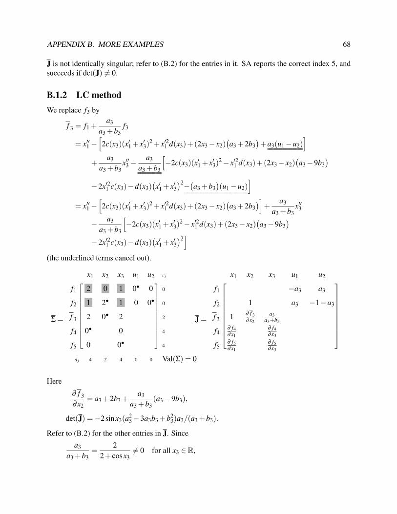
APPENDIX B. MORE EXAMPLES 68
J is not identically singular; refer to (B.2) for the entries in it. SA reports the correct index 5, andsucceeds if det(J) 6= 0.
B.1.2 LC methodWe replace f3 by
f 3 = f1 +a3
a3 +b3f3
= x′′1−[2c(x3)(x′1 + x′3)
2 + x′21 d(x3)+(2x3− x2)(a3 +2b3
)+a3(u1−u2)
]+
a3
a3 +b3x′′3−
a3
a3 +b3
[−2c(x3)(x′1 + x′3)
2− x′21 d(x3)+(2x3− x2)(a3−9b3
)−2x′21 c(x3)−d(x3)
(x′1 + x′3
)2−(a3 +b3
)(u1−u2)
]= x′′1−
[2c(x3)(x′1 + x′3)
2 + x′21 d(x3)+(2x3− x2)(a3 +2b3
)]+
a3
a3 +b3x′′3
− a3
a3 +b3
[−2c(x3)(x′1 + x′3)
2− x′21 d(x3)+(2x3− x2)(a3−9b3
)−2x′21 c(x3)−d(x3)
(x′1 + x′3
)2]
(the underlined terms cancel out).
Σ =
x1 x2 x3 u1 u2 ci
f1 2 0 1 0• 0 0
f2 1 2• 1 0 0• 0
f 3 2 0• 2 2
f4 0• 0 4
f5 0 0• 4
d j 4 2 4 0 0 Val(Σ) = 0
J =
x1 x2 x3 u1 u2
f1 −a3 a3
f2 1 a3 −1−a3
f 3 1 ∂ f 3∂x2
a3a3+b3
f4∂ f4∂x1
∂ f4∂x3
f5∂ f5∂x1
∂ f5∂x3
Here
∂ f 3∂x2
= a3 +2b3 +a3
a3 +b3(a3−9b3),
det(J) =−2sinx3(a23−3a3b3 +b2
3)a3/(a3 +b3).
Refer to (B.2) for the other entries in J. Since
a3
a3 +b3=
22+ cosx3
6= 0 for all x3 ∈ R,
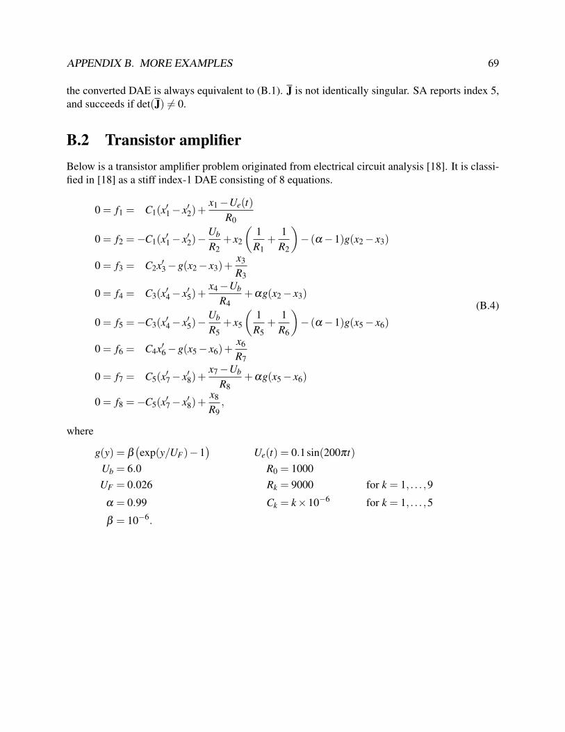
APPENDIX B. MORE EXAMPLES 69
the converted DAE is always equivalent to (B.1). J is not identically singular. SA reports index 5,and succeeds if det(J) 6= 0.
B.2 Transistor amplifierBelow is a transistor amplifier problem originated from electrical circuit analysis [18]. It is classi-fied in [18] as a stiff index-1 DAE consisting of 8 equations.
0 = f1 = C1(x′1− x′2)+x1−Ue(t)
R0
0 = f2 =−C1(x′1− x′2)−Ub
R2+ x2
(1
R1+
1R2
)− (α−1)g(x2− x3)
0 = f3 = C2x′3−g(x2− x3)+x3
R3
0 = f4 = C3(x′4− x′5)+x4−Ub
R4+αg(x2− x3)
0 = f5 =−C3(x′4− x′5)−Ub
R5+ x5
(1
R5+
1R6
)− (α−1)g(x5− x6)
0 = f6 = C4x′6−g(x5− x6)+x6
R7
0 = f7 = C5(x′7− x′8)+x7−Ub
R8+αg(x5− x6)
0 = f8 =−C5(x′7− x′8)+x8
R9,
(B.4)
where
g(y) = β(exp(y/UF)−1
)Ue(t) = 0.1sin(200πt)
Ub = 6.0 R0 = 1000UF = 0.026 Rk = 9000 for k = 1, . . . ,9
α = 0.99 Ck = k×10−6 for k = 1, . . . ,5
β = 10−6.
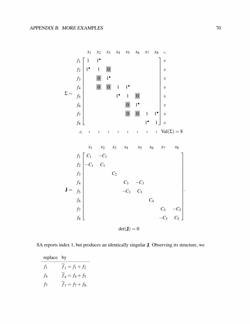
APPENDIX B. MORE EXAMPLES 70
Σ =
x1 x2 x3 x4 x5 x6 x7 x8 ci
f1 1 1• 0
f2 1• 1 0 0
f3 0 1• 0
f4 0 0 1 1• 0
f5 1• 1 0 0
f6 0 1• 0
f7 0 0 1 1• 0
f8 1• 1 0
d j 1 1 1 1 1 1 1 1 Val(Σ) = 8
J =
x1 x2 x3 x4 x5 x6 x7 x8
f1 C1 −C1
f2 −C1 C1
f3 C2
f4 C3 −C3
f5 −C3 C3
f6 C4
f7 C5 −C5
f8 −C5 C5
det(J) = 0
.
SA reports index 1, but produces an identically singular J. Observing its structure, we
replace by
f1 f 1 = f1 + f2
f4 f 4 = f4 + f5
f7 f 7 = f7 + f8.
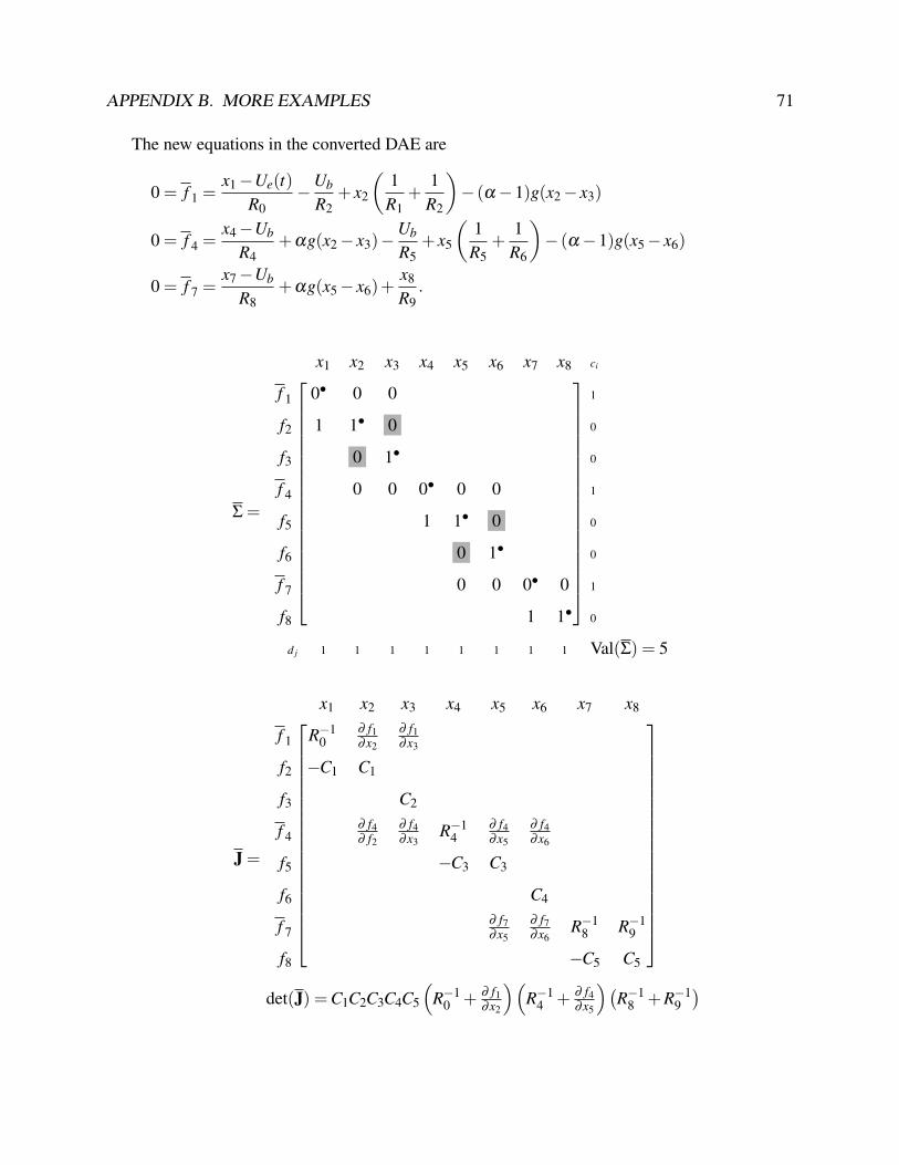
APPENDIX B. MORE EXAMPLES 71
The new equations in the converted DAE are
0 = f 1 =x1−Ue(t)
R0−Ub
R2+ x2
(1
R1+
1R2
)− (α−1)g(x2− x3)
0 = f 4 =x4−Ub
R4+αg(x2− x3)−
Ub
R5+ x5
(1
R5+
1R6
)− (α−1)g(x5− x6)
0 = f 7 =x7−Ub
R8+αg(x5− x6)+
x8
R9.
Σ =
x1 x2 x3 x4 x5 x6 x7 x8 ci
f 1 0• 0 0 1
f2 1 1• 0 0
f3 0 1• 0
f 4 0 0 0• 0 0 1
f5 1 1• 0 0
f6 0 1• 0
f 7 0 0 0• 0 1
f8 1 1• 0
d j 1 1 1 1 1 1 1 1 Val(Σ) = 5
J =
x1 x2 x3 x4 x5 x6 x7 x8
f 1 R−10
∂ f1∂x2
∂ f1∂x3
f2 −C1 C1
f3 C2
f 4∂ f4∂ f2
∂ f4∂x3
R−14
∂ f4∂x5
∂ f4∂x6
f5 −C3 C3
f6 C4
f 7∂ f7∂x5
∂ f7∂x6
R−18 R−1
9
f8 −C5 C5
det(J) =C1C2C3C4C5
(R−1
0 + ∂ f1∂x2
)(R−1
4 + ∂ f4∂x5
)(R−1
8 +R−19)
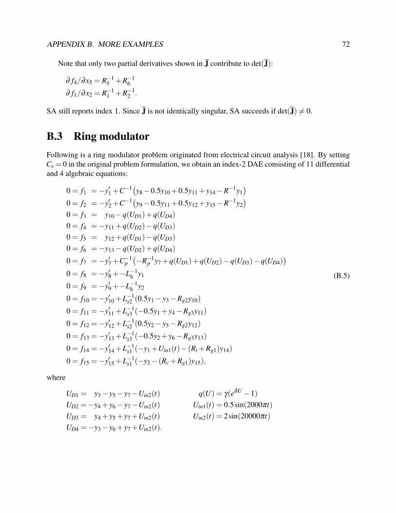
APPENDIX B. MORE EXAMPLES 72
Note that only two partial derivatives shown in J contribute to det(J):
∂ f4/∂x5 = R−15 +R−1
6
∂ f1/∂x2 = R−11 +R−1
2 .
SA still reports index 1. Since J is not identically singular, SA succeeds if det(J) 6= 0.
B.3 Ring modulatorFollowing is a ring modulator problem originated from electrical circuit analysis [18]. By settingCs = 0 in the original problem formulation, we obtain an index-2 DAE consisting of 11 differentialand 4 algebraic equations:
0 = f1 =−y′1 +C−1(y8−0.5y10 +0.5y11 + y14−R−1y1)
0 = f2 =−y′2 +C−1(y9−0.5y11 +0.5y12 + y15−R−1y2)
0 = f3 = y10−q(UD1)+q(UD4)
0 = f4 =−y11 +q(UD2)−q(UD3)
0 = f5 = y12 +q(UD1)−q(UD3)
0 = f6 =−y13−q(UD2)+q(UD4)
0 = f7 =−y′7 +C−1p(−R−1
p y7 +q(UD1)+q(UD2)−q(UD3)−q(UD4))
0 = f8 =−y′8 +−L−1h y1
0 = f9 =−y′9 +−L−1h y2
0 = f10 =−y′10 +L−1s2 (0.5y1− y3−Rg2y10)
0 = f11 =−y′11 +L−1s3 (−0.5y1 + y4−Rg3y11)
0 = f12 =−y′12 +L−1s2 (0.5y2− y5−Rg2y12)
0 = f13 =−y′13 +L−1s3 (−0.5y2 + y6−Rg3y13)
0 = f14 =−y′14 +L−1s1 (−y1 +Uin1(t)− (Ri +Rg1)y14)
0 = f15 =−y′15 +L−1s1 (−y2− (Rc +Rg1)y15),
(B.5)
where
UD1 = y3− y5− y7−Uin2(t) q(U) = γ(eδU −1)UD2 =−y4 + y6− y7−Uin2(t) Uin1(t) = 0.5sin(2000πt)UD3 = y4 + y5 + y7 +Uin2(t) Uin2(t) = 2sin(20000πt)UD4 =−y3− y6 + y7 +Uin2(t).
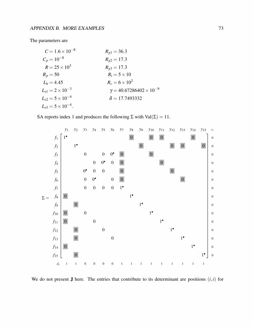
APPENDIX B. MORE EXAMPLES 73
The parameters are
C = 1.6×10⁻⁸ Rg1 = 36.3
Cp = 10−8 Rg2 = 17.3
R = 25×103 Rg3 = 17.3Rp = 50 Ri = 5×10
Lh = 4.45 Rc = 6×10²
Ls1 = 2×10⁻³γ = 40.67286402×10⁻⁹
Ls2 = 5×10⁻⁴δ = 17.7493332
Ls3 = 5×10⁻⁴.
SA reports index 1 and produces the following Σ with Val(Σ) = 11.
Σ =
y1 y2 y3 y4 y5 y6 y7 y8 y9 y10 y11 y12 y13 y14 y15 ci
f1 1• 0 0 0 0 0
f2 1• 0 0 0 0 0
f3 0 0 0• 0 0 0
f4 0 0• 0 0 0 0
f5 0• 0 0 0 0 0
f6 0 0• 0 0 0 0
f7 0 0 0 0 1• 0
f8 0 1• 0
f9 0 1• 0
f10 0 0 1• 0
f11 0 0 1• 0
f12 0 0 1• 0
f13 0 0 1• 0
f14 0 1• 0
f15 0 1• 0
d j 1 1 0 0 0 0 1 1 1 1 1 1 1 1 1
We do not present J here. The entries that contribute to its determinant are positions (i, i) for
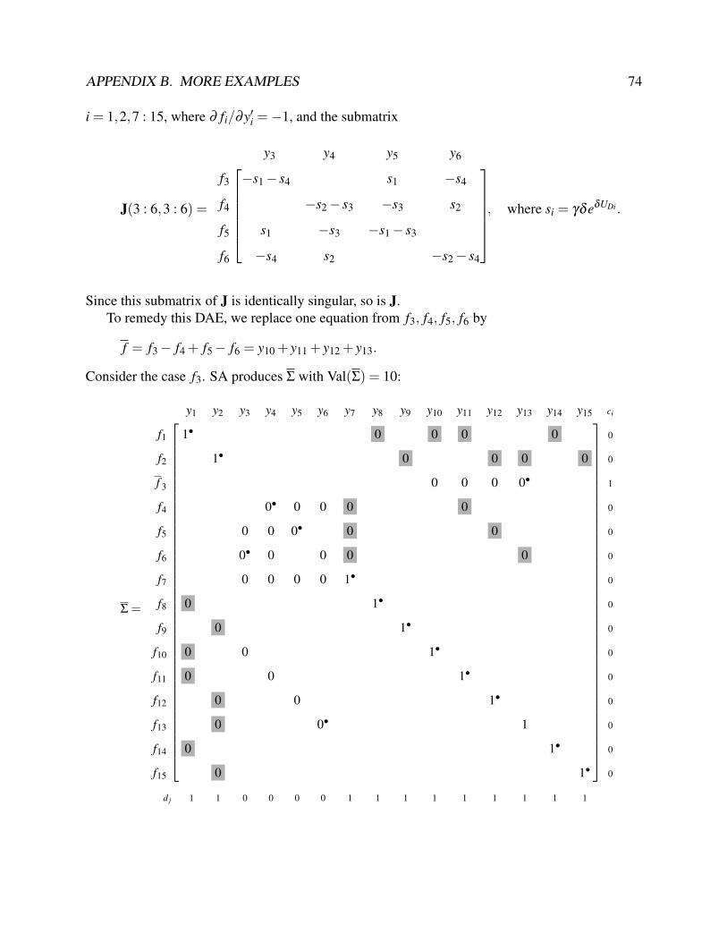
APPENDIX B. MORE EXAMPLES 74
i = 1,2,7 : 15, where ∂ fi/∂y′i =−1, and the submatrix
J(3 : 6,3 : 6) =
y3 y4 y5 y6
f3 −s1− s4 s1 −s4
f4 −s2− s3 −s3 s2
f5 s1 −s3 −s1− s3
f6 −s4 s2 −s2− s4
, where si = γδeδUDi.
Since this submatrix of J is identically singular, so is J.To remedy this DAE, we replace one equation from f3, f4, f5, f6 by
f = f3− f4 + f5− f6 = y10 + y11 + y12 + y13.
Consider the case f3. SA produces Σ with Val(Σ) = 10:
Σ =
y1 y2 y3 y4 y5 y6 y7 y8 y9 y10 y11 y12 y13 y14 y15 ci
f1 1• 0 0 0 0 0
f2 1• 0 0 0 0 0
f 3 0 0 0 0• 1
f4 0• 0 0 0 0 0
f5 0 0 0• 0 0 0
f6 0• 0 0 0 0 0
f7 0 0 0 0 1• 0
f8 0 1• 0
f9 0 1• 0
f10 0 0 1• 0
f11 0 0 1• 0
f12 0 0 1• 0
f13 0 0• 1 0
f14 0 1• 0
f15 0 1• 0
d j 1 1 0 0 0 0 1 1 1 1 1 1 1 1 1
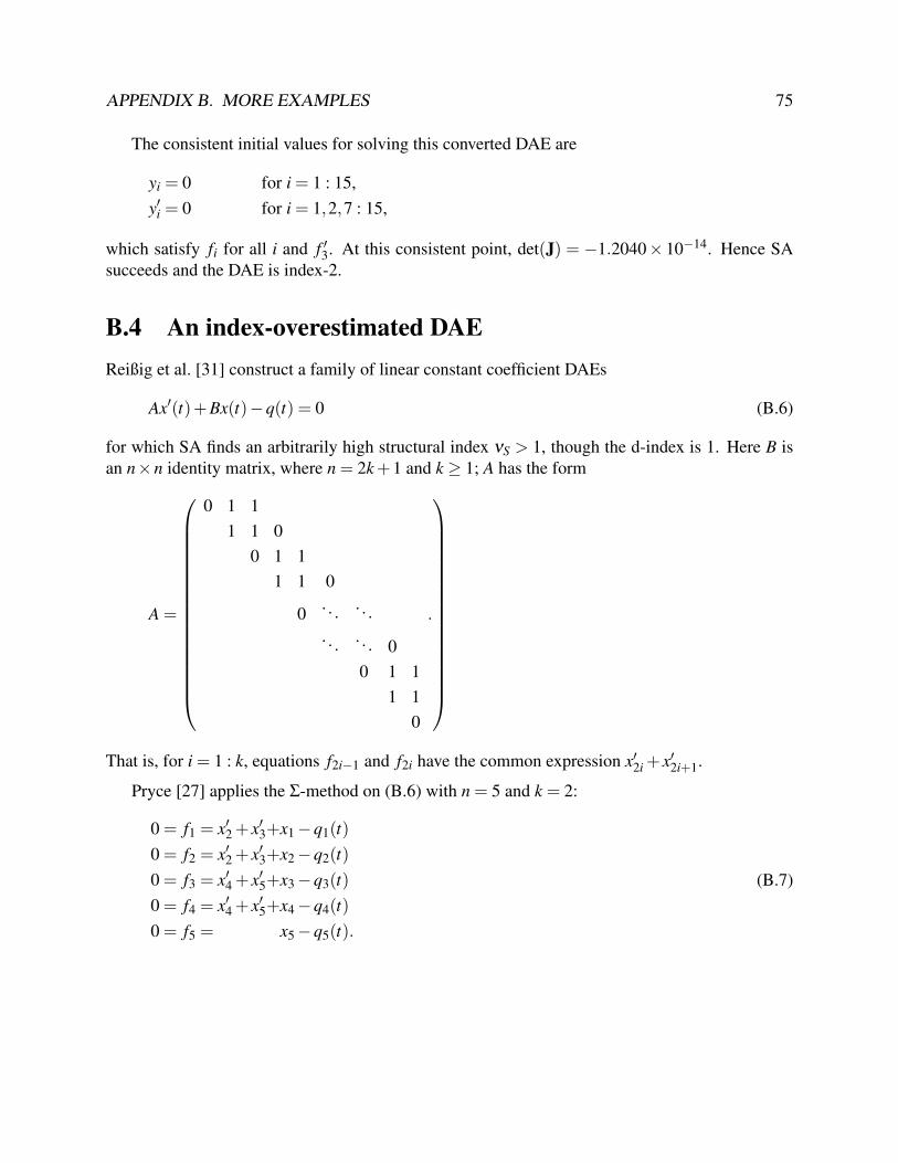
APPENDIX B. MORE EXAMPLES 75
The consistent initial values for solving this converted DAE are
yi = 0 for i = 1 : 15,y′i = 0 for i = 1,2,7 : 15,
which satisfy fi for all i and f ′3. At this consistent point, det(J) = −1.2040× 10⁻¹⁴. Hence SAsucceeds and the DAE is index-2.
B.4 An index-overestimated DAEReißig et al. [31] construct a family of linear constant coefficient DAEs
Ax′(t)+Bx(t)−q(t) = 0 (B.6)
for which SA finds an arbitrarily high structural index νS > 1, though the d-index is 1. Here B isan n×n identity matrix, where n = 2k+1 and k ≥ 1; A has the form
A =
0 1 11 1 0
0 1 11 1 0
0 . . . . . .. . . . . . 0
0 1 11 1
0
.
That is, for i = 1 : k, equations f2i−1 and f2i have the common expression x′2i + x′2i+1.
Pryce [27] applies the Σ-method on (B.6) with n = 5 and k = 2:
0 = f1 = x′2 + x′3+x1−q1(t)0 = f2 = x′2 + x′3+x2−q2(t)0 = f3 = x′4 + x′5+x3−q3(t)0 = f4 = x′4 + x′5+x4−q4(t)0 = f5 = x5−q5(t).
(B.7)

APPENDIX B. MORE EXAMPLES 76
Σ =
x1 x2 x3 x4 x5 ci
f1 0• 1 1 0
f2 1• 1 0
f3 0• 1 1 1
f4 1• 1 1
f5 0• 2
d j 0 1 1 2 2 Val(Σ) = 2
J =
x1 x2 x3 x4 x5
f1 1 1 1
f2 1 1
f3 1 1 1
f4 1 1
f5 1
det(J) = 1
The method succeeds with det(J) = 1 but reports νS = 3 different from νd = 1; this occurs inPantelides’s SA as well. We illustrate below how to fix this index overestimation problem for(B.7).
Observing the structure of A, we
replace by
f1 f 1 = f1− f2
f3 f 3 = f3− f4.
The converted DAE is
0 = f 1 = x1− x2−q1(t)+q2(t)0 = f2 = x′2 + x′3 + x2−q2(t)
0 = f 3 = x3− x4−q3(t)+q4(t)0 = f4 = x′4 + x′5 + x4−q4(t)0 = f5 = x5−q5(t).
(B.8)
Σ =
x1 x2 x3 x4 x5 ci
f 1 0• 0 1
f2 1• 1 0
f 3 0• 0 1
f4 1• 1 0
f5 0• 1
d j 1 1 1 1 1 Val(Σ) = 2
J =
x1 x2 x3 x4 x5
f 1 1 −1
f2 1 1
f 3 1 −1
f4 1 1
f5 1
det(J) = 1
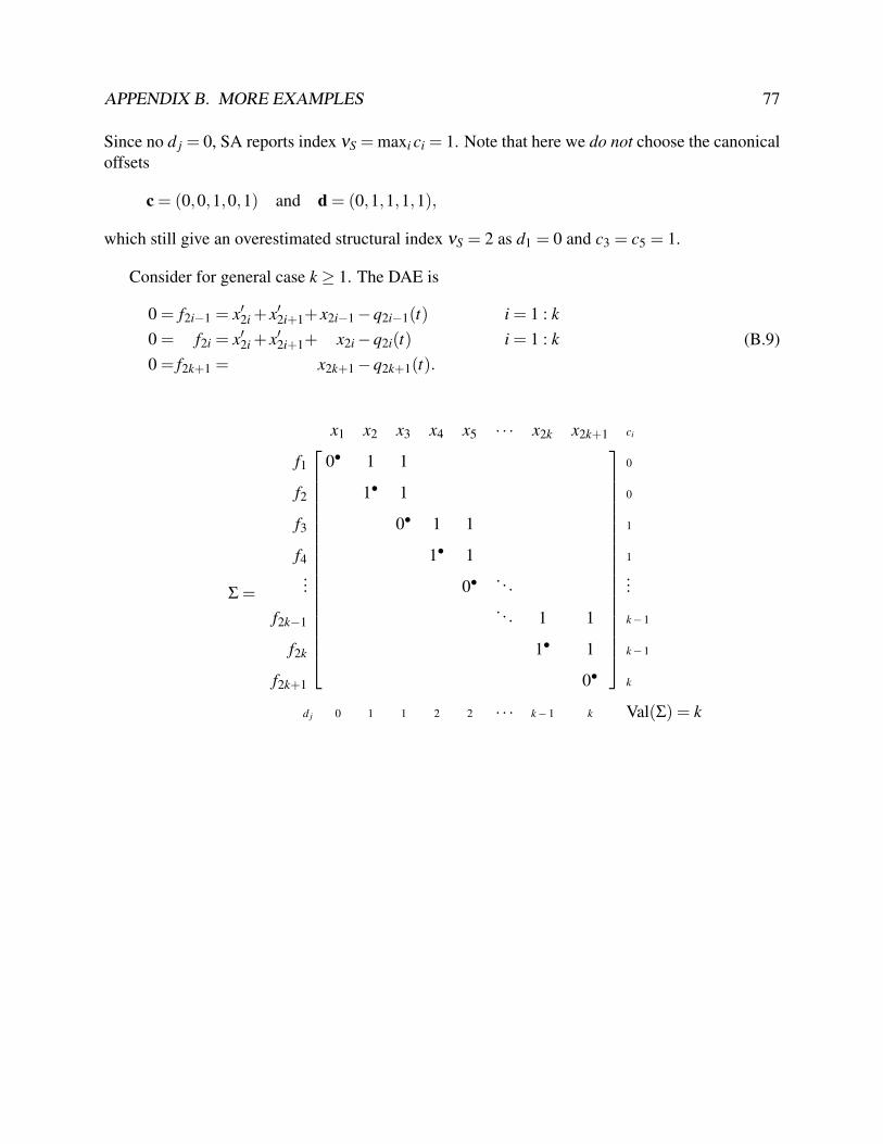
APPENDIX B. MORE EXAMPLES 77
Since no d j = 0, SA reports index νS = maxi ci = 1. Note that here we do not choose the canonicaloffsets
c = (0,0,1,0,1) and d = (0,1,1,1,1),
which still give an overestimated structural index νS = 2 as d1 = 0 and c3 = c5 = 1.
Consider for general case k ≥ 1. The DAE is
0 = f2i−1 = x′2i + x′2i+1+ x2i−1−q2i−1(t) i = 1 : k0 = f2i = x′2i + x′2i+1+ x2i−q2i(t) i = 1 : k0 = f2k+1 = x2k+1−q2k+1(t).
(B.9)
Σ =
x1 x2 x3 x4 x5 · · · x2k x2k+1 ci
f1 0• 1 1 0
f2 1• 1 0
f3 0• 1 1 1
f4 1• 1 1
... 0• . . . ...
f2k−1. . . 1 1 k−1
f2k 1• 1 k−1
f2k+1 0• k
d j 0 1 1 2 2 · · · k−1 k Val(Σ) = k

APPENDIX B. MORE EXAMPLES 78
J =
x1 x2 x3 x4 x5 · · · x2k x2k+1
f1 1 1 1
f2 1 1
f3 1 1 1
f4 1 1... . . . . . .
f2k−1 1 1 1
f2k 1 1
f2k+1 1
det(J) = 1
SA succeeds and reports structural index k+1.To remedy this index overestimation, we repeat the same strategy used above: for i = 1 : k, we
replace f2i−1 by f 2i−1 = f2i−1− f2i. The converted DAE is
0 = f 2i−1 = x2i−1− x2i−q2i−1(t)+q2i(t) i = 1 : k0 = f2i = x′2i + x′2i+1 + x2i−q2i(t) i = 1 : k0 = f2k+1 = x2k+1−q2k+1(t).
(B.10)
Σ =
x1 x2 x3 x4 x5 · · · x2k x2k+1 ci
f 1 0• 0 1
f2 1• 1 0
f 3 0• 0 1
f4 1• 1 0
... 0• . . . ...
f 2k−1. . . 0 1
f2k 1• 1 0
f2k+1 0• 1
d j 1 1 1 1 1 · · · 1 1 Val(Σ) = k
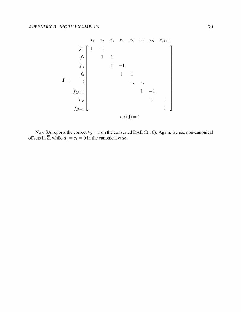
APPENDIX B. MORE EXAMPLES 79
J =
x1 x2 x3 x4 x5 · · · x2k x2k+1
f 1 1 −1
f2 1 1
f 3 1 −1
f4 1 1... . . . . . .
f 2k−1 1 −1
f2k 1 1
f2k+1 1
det(J) = 1
Now SA reports the correct νS = 1 on the converted DAE (B.10). Again, we use non-canonicaloffsets in Σ, while d1 = c1 = 0 in the canonical case.
Bibliography
[1] U. M. ASCHER AND L. R. PETZOLD, Computer Methods for Ordinary Differential Equa-tions and Differential-Algebraic Equations, SIAM, Philadelphia, 1998.
[2] R. BARRIO, Performance of the Taylor series method for ODEs/DAEs, Appl. Math. Comp.,163 (2005), pp. 525–545.
[3] K. BRENAN, S. CAMPBELL, AND L. PETZOLD, Numerical Solution of Initial-Value Prob-lems in Differential-Algebraic Equations, SIAM, Philadelphia, second ed., 1996.
[4] S. L. CAMPBELL AND C. W. GEAR, The index of general nonlinear DAEs, NumerischeMathematik, 72 (1995), pp. 173–196.
[5] S. L. CAMPBELL AND E. GRIEPENTROG, Solvability of general differential algebraic equa-tions, SIAM J. Sci. Comput., 16 (1995), pp. 257–270.
[6] S. CHOWDHRY, H. KRENDL, AND A. A. LINNINGER, Symbolic numeric index analysisalgorithm for differential algebraic equations, Industrial & engineering chemistry research,43 (2004), pp. 3886–3894.
[7] I. S. DUFF AND C. W. GEAR, Computing the structural index, SIAM Journal on Algebraicand Discrete Methods, 7 (1986), p. 594603.
[8] D. ESTVEZ SCHWARZ AND R. LAMOUR, Diagnosis of singular points of properly stateddaes using automatic differentiation, Numerical Algorithms, (2015), pp. 1–29.
[9] C. W. GEAR, Differential-algebraic equation index transformations, SIAM Journal on Sci-entific and Statistical Computing, 9 (1988), pp. 39–47.
[10] , Differential algebraic equations, indices, and integral algebraic equations, SIAM Jour-nal on Numerical Analysis, 27 (1990), pp. 1527–1534.
[11] E. GRIEPENTROG AND R. MARZ, Differential-algebraic equations and their numericaltreatment, in Teubner-Texte zur Mathematik [Teubner Texts in Mathematics], 88., BSB B. G.Teubner Verlagsgesellschaft, Leipzig, 1986. With German, French and Russian summaries.
80
BIBLIOGRAPHY 81
[12] A. GRIEWANK AND A. WALTHER, On the efficient generation of Taylor expansions forDAE solutions by automatic differentiation, in Applied Parallel Computing. State of the Artin Scientific Computing, Springer, 2006, pp. 1089–1098.
[13] E. HAIRER AND G. WANNER, Solving Ordinary Differential Equations II. Stiff andDifferential– Algebraic Problems, Springer Verlag, Berlin, 1991.
[14] A. C. HINDMARSH, P. N. BROWN, K. E. GRANT, S. L. LEE, R. SERBAN, D. E. SHU-MAKER, AND C. S. WOODWARD, Sundials: Suite of nonlinear and differential/algebraicequation solvers, ACM Trans. Math. Softw., 31 (2005), pp. 363–396.
[15] J. HOEFKENS, Rigorous Numerical Analysis with High-Order Taylor Models, PhD thesis,Department of Mathematics and Department of Physics and Astronomy, Michigan State Uni-versity, East Lansing, MI 48824, August 2001.
[16] P. KUNKEL AND V. MEHRMANN, Differential-Algebraic Equations — Analysis and Numer-ical Solution, EMS Publishing House, Zurich, Switzerland, 2006.
[17] S. E. MATTSSON AND G. SODERLIND, Index reduction in differential-algebraic equationsusing dummy derivatives, SIAM J. Sci. Comput., 14 (1993), pp. 677–692.
[18] F. MAZZIA AND F. IAVERNARO, Test set for initial value problem solvers, Tech. Rep. 40,Department of Mathematics, University of Bari, Italy, 2003. http://pitagora.dm.uniba.it/˜testset/.
[19] R. MCKENZIE, J. D. PRYCE, G. TAN, AND N. S. NEDIALKOV, Structural analysis anddummy derivatives for differential-algebraic equations, 2015. In preparation.
[20] N. S. NEDIALKOV AND J. D. PRYCE, Solving differential-algebraic equations by Taylorseries (I): Computing Taylor coefficients, BIT Numerical Mathematics, 45 (2005), pp. 561–591.
[21] N. S. NEDIALKOV AND J. D. PRYCE, Solving differential-algebraic equations by Taylorseries (II): Computing the system Jacobian, BIT Numerical Mathematics, 47 (2007), pp. 121–135.
[22] , Solving differential algebraic equations by Taylor series (III): the DAETS code, JNA-IAM J. Numer. Anal. Indust. Appl. Math, 3 (2008), pp. 61–80.
[23] N. S. NEDIALKOV, J. D. PRYCE, AND G. TAN, DAESA — a Matlab tool for structuralanalysis of DAEs: Software, ACM Transactions on Mathematical Software, to appear (2015).15 pages.
[24] N. S. NEDIALKOV, G. TAN, AND J. D. PRYCE, Exploiting fine block triangularization andquasilinearity in differential-algebraic equation systems, arXiv:1411.4128, (2014). 18 pages.
BIBLIOGRAPHY 82
[25] C. C. PANTELIDES, The consistent initialization of differential-algebraic systems, SIAM. J.Sci. Stat. Comput., 9 (1988), pp. 213–231.
[26] J. D. PRYCE, Solving high-index DAEs by Taylor Series, Numerical Algorithms, 19 (1998),pp. 195–211.
[27] J. D. PRYCE, A simple structural analysis method for DAEs, BIT Numerical Mathematics,41 (2001), pp. 364–394.
[28] J. D. PRYCE, N. S. NEDIALKOV, AND G. TAN, Graph theory, irreducibility, and structuralanalysis of differential-algebraic equation systems, arXiv:1411.4129, (2014). 24 pages.
[29] J. D. PRYCE, N. S. NEDIALKOV, AND G. TAN, DAESA — a Matlab tool for structuralanalysis of DAEs: Theory, ACM Transactions on Mathematical Software, to appear (2015).20 pages.
[30] P. J. RABIER AND W. C. RHEINBOLDT, A general existence and uniqueness theory forimplicit differential-algebraic equations, Differential Integral Equations, 4 (1991), pp. 563–582.
[31] G. REISSIG, W. S. MARTINSON, AND P. I. BARTON, Differential–algebraic equations ofindex 1 may have an arbitrarily high structural index, SIAM J. Sci. Comput., 21 (1999),pp. 1987–1990.
[32] W. C. RHEINBOLDT, Differential-algebraic systems as differential equations on manifolds,Mathematics of computation, 43 (1984), pp. 473–482.
[33] L. SCHOLZ AND A. STEINBRECHER, A combined structural-algebraic approach for theregularization of coupled systems of DAEs, Tech. Rep. 30, Reihe des Instituts fur MathematikTechnische Universitat Berlin, Berlin, Germany, 2013.
[34] R. D. P. SOARES AND A. R. SECCHI, Structural analysis for static and dynamic models,Mathematical and Computer Modelling, 55 (2012), pp. 1051–1067.
[35] J. UNGER, A. KRONER, AND W. MARQUARDT, Structural analysis of differential-algebraicequation systems – theory and applications, Computers & Chemical Engineering, 19 (1995),pp. 867–882.