Course information:-------------------1. Course name: Introductory Ocean Sciences2. Department: Estuarine and Ocean Sciences, SMAST3. Number: 1054. Cluster requirement: Science of the Natural World

Faculty information:--------------------5. Name: Miles Sundermeyer6. Email: msundermeyer@umassd.edu7. Phone: 508-999-8892

Required components:--------------------8. Master syllabus: http:///webroots/www.umassd.edu/genedchecklist/holding/master_syllabus_mar105.doc9. Course overview statement:Introductory Ocean Sciences - MAR 105

This course is intended to convey the following essential principles of ocean sciences in an enjoyable learning environment: (i) the earth has one big ocean with many features; (ii) the ocean and life within in help shape the features of the Earth; (iii) the ocean is a major influence on weather and climate; (iv) the ocean makes Earth habitable; (v) the ocean supports a great diversity of life and ecosystems; (vi) the ocean and humans are inextricably interconnected; (vii) sustainability of ocean resources depends on our understanding of those resources and their potential and limitations.

The course has to option be offered as a traditional face-to-face lecture course, using blended learning, or entirely online. Weekly topics familiarize students with the many different facets of ocean sciences, including physical, biological, chemical, and geological oceanography, as well as the ocean’s relation to climate and ocean policy. Various examples are also given of ocean instruments used for sampling, measurement, and analysis, along with how the data are used in scientific inquiry and to address societally relevant questions and problems. Homework assignments include reading and answering questions about topics discussed in lecture, text, and/or supplemental reading materials. Assignments also include group investigations using MyCourses, the internet, and other resources. The student completing the course will be an "ocean literate" person.

Weekly learning topics range from a general overview of the world oceans within the Earth system, to a progression of different sub-disciplines of oceanography, from tectonics, marine sediments, ocean/atmospheres interaction, ocean physics, biology and chemistry, climate, and global policy issues. Each week includes readings from the course textbook, plus supplementary readings and Investigations that students work on either individually or in small groups (e.g., discussion groups).

This course is an ideal fit to the University Studies requirement under Cluster 2A: The Natural World. Topics covered in the course address each of the University Studies outcomes, regarding 1) recounting fundamental concepts across the various facets of ocean sciences, 2) explaining how scientific data are used to draw conclusions about the world oceans and climate, 3) using quantitative information to draw conclusions and communicate these conclusions in writing, and 4) synthesizing various aspects of ocean science to identify solutions to a variety of societally relevant ocean and climate related problems. Weekly assignments provide regular feedback to instructor(s) and external assessors on how well students are achieving both course specific and University Studies

learning outcomes, which in this case have significant overlap. Two exams (mid-term and final) test student’s cumulative learning outcomes and learning retention in these areas. Last, as the course may be offered either face-to-face, using blended learning, or fully online, the course has the ability to reach a wide range of students at UMass Dartmouth, from those residing on campus, to continuing education, to fully online learners. Hence the course provides maximum flexibility for students seeking to fulfill their University Studies 2A requirement.

10. Signed faculty and chair sponsor sheet: sent separately.11. Official course catalog description for the course:Essential principles of ocean sciences. This course explores topics such as how the ocean and life in the ocean shape the features of the Earth; the ocean as a major influence on weather and climate; how the ocean supports a great diversity of life and ecosystems; and how the sustainability of ocean resources depends on our understanding of those resources and their potential and limitations. Various examples of ocean instruments used for sampling and measurements are introduced. 12. Course approval form: not entered.

Master SyllabusCourse: MAR-105: Introductory Ocean Sciences

Cluster Requirement: 2A

This University Studies Master Syllabus serves as a guide and standard for all instructors teaching an approved course in the University Studies program. Individual instructors have full academic freedom in teaching their courses, but as a condition of course approval, agree to focus on the outcomes listed below, to cover the identified material, to use these or comparable assignments as part of the course work, and to make available the agreed-upon artifacts for assessment of learning outcomes.

Course Overview:

This course is intended to convey the following essential principles of ocean sciences in an enjoyable learning environment: (i) the earth has one big ocean with many features; (ii) the ocean and life within in help shape the features of the Earth; (iii) the ocean is a major influence on weather and climate; (iv) the ocean makes Earth habitable; (v) the ocean supports a great diversity of life and ecosystems; (vi) the ocean and humans are inextricably interconnected; (vii) sustainability of ocean resources depends on our understanding of those resources and their potential and limitations.

This course has to option be offered as a traditional face-to-face lecture course, using blended learning, or entirely online. Weekly topics will familiarize students with the many different facets of ocean sciences, including physical, biological, chemical, and geological oceanography, as well as the ocean’s relation to climate and ocean policy. Various examples are also given of ocean instruments used for sampling, measurement, and analysis, along with how the data are used in scientific inquiry and to address societally relevant questions and problems. Homework assignments include reading and answering questions about topics discussed in lecture, text, and/or supplemental reading materials. Assignments also include group investigations using MyCourses, the internet, and other resources. The student completing the course will be an "ocean literate" person.

Learning Outcomes:

Course-Specific Learning Outcomes: Students will be able to explain basic oceanographic principles within the different sub-disciplines of

physical, biological, chemical, and geological oceanography, and how they relate to global climate. Students will be able to describe how science (particularly ocean science) works, how scientific theories

are advanced, and how science is an evolving understanding of the world around us. Students will be able to discuss the science underpinning of oceanography and its interaction with the

atmosphere and global climate. Students will be able to give examples of the role of the ocean in the Earth System in the context of

ocean related environmental issues and current events.

University Studies Learning Outcomes:Cluster 2 –The Natural World: Scientific Inquiry and Understanding

A. Science of the Natural World

After completing this course, students will be able to: 1. Recount the fundamental concepts and methods in one or more specific fields of science. 2. Explain how the scientific method is used to produce knowledge.

3. Successfully use quantitative information to communicate their understanding of scientific knowledge.

4. Use appropriate scientific knowledge to solve problems.

Examples of Texts and/or Assigned Readings:

The current incarnation of this course uses the American Meteorological Society licensed Ocean Studies course materials for traditional face-to-face, blended learning, and online options of the course. The following are the primary resources for this incarnation:

Ocean Studies: Introduction to Oceanography, 3rd ed., Joseph Moran, published by The American Meteorological Society

AMS Ocean Studies Investigations Manual, published by The American Meteorological Society

Various excerpts from the American Meteorological Society website under their Ocean Studies course: http://www.ametsoc.org/amsedu/online/oceaninfo/

A previous incarnation of this course also used the following text, which is equally appropriate for the face-to-face version of the course:

Alternate Text: Oceans. An Illustrated Reference, by Dorrik Stow, Southampton Oceanography Centre, U.K.; Univ. Chicago Press, 2006

Example Learning Activities and Assignments:

Per the course syllabus (see final attachment of this document), weekly learning topics range from a general overview of the world oceans within the Earth system, to a progression of different sub-disciplines of oceanography, from tectonics, marine sediments, ocean/atmospheres interaction, ocean physics, biology and chemistry, climate, and global policy issues. Each week includes readings from the course textbook, plus supplementary readings and Investigations that students work on either individually or in small groups (e.g., discussion groups). Weekly assessments within the Investigations address each of the University Studies outcomes, regarding 1) recounting fundamental concepts across the various facets of ocean sciences, 2) explaining how scientific data are used to draw conclusions about the world oceans and climate, 3) using quantitative information to draw conclusions and communicate these conclusions in writing, and 4) synthesizing various aspects of ocean science to identify solutions to a variety of societally relevant ocean and climate related problems. Two exams (mid-term and final) will test student’s cumulative learning outcomes and learning retention in these areas.

Examples for each of the University Studies Outcomes in the included course material examples are as follows:

1. Recount the fundamental concepts and methods in one or more specific fields of science. Addressed by multiple questions posed in weekly Investigations - examples relating to the ocean’s role in global climate is given in the attached Investigations 1A module.

2. Explain how the scientific method is used to produce knowledge. Each week will highlight one or more ocean related issues, walking students through various data, graphs, and conceptual scientific steps to draw conclusions about causes, effects, and interactions between various components of the ocean/Earth system. An example for eutrophication/ocean dead zones in the Gulf of Mexico is provided in the attached Current Oceans Study module 1.

3. Successfully use quantitative information to communicate their understanding of scientific knowledge.

Also addressed in weekly Investigations and Current Oceans Study modules, where students are asked to read and/or interpret various graphs and data and answer questions about them.

4. Use appropriate scientific knowledge to solve problems. In each of the weekly modules, various topics addressed are brought back to bear on real-world current scientific and policy questions and issues. This provides students with case examples of how scientific knowledge is used to solve problems, which in this course relate to the oceans and climate. An example in the attached learning module is how the Gulf of Mexico “dead zone” is regulated and targeted for nutrient reduction by the U.S. Nutrient Management Task Force. Students understanding of how the scientific process works to addres real-world problems is reinforced throughout the course via such readings and case examples, and is tested both in weekly Investigations and on mid-term and final exams.

Weekly recitation / office hour sessions are held by the Professor and a TA to provide guidance/feedback on homework assignments, and provide general help and further discussion on concepts presented in the course. Overall, textbook readings, lecture, weekly Investigations, and supplemental readings and Current Ocean Studies modules are designed to work in concert to address the primary learning outcomes relevant to University Studies 2A. Thus, rather than having specific modules and/or assignments geared toward just one learning outcome, the course structure integrates all course materials within a given week to address and integrate multiple learning outcomes in a synthesized manner.

Regarding artifacts for assessing how well students have met the different course and University Studies learning outcomes, weekly assignments within the Investigations modules will provide a running record over the course of the semester for how well students are achieving the various outcomes. Mid-term and final exams will further provide a more concise and cumulative assessment of how students are meeting the learning outcomes for the course overall.

Example supplemental readings, assignments and assessments provided on the following pages. Additional information regarding the AMS Ocean Studies course can be found at: https://www.ametsoc.org/amsedu/online/oceaninfo/

EXAMPLE WEEKLY SUPPLEMENTAL READING ASSIGNEMNT AND QUESTIONS

Note: This Investigation is the same as AMS Ocean Studies' Current Ocean Studies 1 from Preview Week. Participants only need to complete the Current Ocean Studies once. Do Now: 1. Print this file, if directed by your instructor. 2. Read the Weekly Ocean News file, print if directed to do so by your instructor.

(Note: Check the AMS Ocean Studies website during the week as breaking ocean news stories may have been added.)

Welcome to AMS Ocean Studies. This is the first of weekly Current Ocean Studies which supplement and build upon the corresponding chapter investigations of the AMS Ocean Studies Investigations Manual. We hope your use of current environmental information will become an engaging experience. We encourage your exploration of the AMS Ocean Studies website products. To Do Investigation: 1. Reference: Chapter 1 in the AMS Ocean Studies text. 2. Complete Investigations 1A and 1B in the AMS Ocean Studies Investigations Manual as directed by your

instructor. 3. Complete this online-delivered Current Ocean Studies activity if directed by your instructor. ________________________________________________________________________ Welcome to the first online Current Ocean Studies component of this course. Current Ocean Studies components accompany every chapter of study and typically are brief case studies of real-world recent, current, or ongoing oceanic situations. Introduction: In December 2008, the National Research Council (NRC) published a report urging the U.S. Environmental Protection Agency and the U.S. Department of Agriculture to jointly establish an initiative leading to the mitigation (reduction) of nutrient pollution in the Mississippi River basin and the northern Gulf of Mexico. The NRC report called for immediate government action to reduce urban and Midwest farmland runoff blamed for feeding a broad and expanding lifeless swath of water, called a dead zone, which forms off both the Louisiana and northeastern Texas coasts every summer. A prime example of the interconnectedness of ocean, land, and impacts of human activity in the Earth system is the increase in number and intensity of such dead zones. Dead zones are ocean areas where dissolved oxygen in bottom and near-bottom waters declines to deadly proportions. Such areas of the seafloor, with too little oxygen for most marine life, are produced when excess nutrients, especially nitrogen and phosphorus compounds, enter coastal surface waters and spur algal blooms. When the algae

die, they sink to the seafloor. Their decomposition consumes the dissolved oxygen, leaving a “hypoxic” (low oxygen) or “anoxic” (no oxygen) environment lethal to many marine species.

Ocean dead zones are primarily coastal and estuarine phenomena. The first to be identified was reported in the 1930s in the Chesapeake Bay estuary system. (Chesapeake Bay’s late July 2011 dead zone covered a third of the Bay and is expected to become the bay’s largest.) It has been estimated that there are nearly 500 dead zones existing worldwide (see http://www.eurekalert.org/pub_releases/2008-08/viom-ssc081108.php and http://www.wri.org/project/eutrophication/map). Most are seasonal, as exemplified by the largest dead zone in the United States which expands off the coast of Louisiana and Texas in late spring and summer. It results from huge quantities of nutrients originating as farm fertilizers and organic wastes carried by the Mississippi River system to the Gulf of Mexico. Figure 1 displays the drainage system of the Mississippi River, including its tributaries and major distributary (Louisiana’s Atchafalaya River). This system is the 3rd largest in the world, after the Amazon and Congo, and drains about 40% of the contiguous U.S. Parts or all of 31 states, and two Canadian provinces, drain into the Mississippi River.

Figure 1. The Mississippi-Atchafalaya River Basin and general position of a typical summer’s Gulf of Mexico “dead zone” (in red). [EPA]

1. It can be seen in Figure 1 that Iowa farmers fertilizing their land to increase corn crop yield are contributing to a key stressor on marine ecosystems over a thousand miles away. This demonstrates clearly that human activity far from the ocean [(can)(cannot)] have dramatic effects on the ocean.

2. Figure 2 depicts how the Gulf of Mexico dead zone forms. During spring, warm Mississippi River water flows into the Gulf and [(floats over)(sinks under)] the more dense seawater. The resulting surface water layer prevents convection and replenishment of dissolved oxygen in seawater at greater depths from the overlying atmosphere.

Figure 2. How the Dead Zone Forms. [The Times-Picayune, http://blog.nola.com/graphics/deadzone_how061007.gif]

View an animation, entitled “The Dead Zone: Nutrient Runoff Creates Hypoxia in the Gulf of Mexico”, by NOAA’s Environmental Visualization Laboratory, at http://www.nnvl.noaa.gov/MediaDetail.php?MediaID=84&MediaTypeID=2 that describes the formation of a dead zone. 3. The animation of satellite imagery shows evidence that nutrients delivered by the Mississippi River into

the Gulf of Mexico are generally carried by coastal currents [(eastward towards Florida)(westward towards Texas)]. The nutrients then produce algae (phytoplankton) blooms.

Another Flash animation describing the nutrient process that leads to hypoxia in the northern waters of the Gulf of Mexico can be found at: http://www.gulfhypoxia.net/Overview/hypoxia_flash.asp. 4. The nutrients from the Mississippi River system, including those from fertilizer runoff and from sewage

discharges, ignite algal blooms in the surface water warmed by the increasingly intense sunlight during spring that remains strong into summer. The dead algae then sink, settle to the ocean bottom, and decompose. The decomposition process results in the [(loss)(gain)] of dissolved oxygen in the deeper seawater.

Dissolved oxygen is an essential ingredient for sustaining life in the marine food chain. With little or no oxygen, commercially important fish and shellfish (e.g., crabs and oysters) as well as non-commercially important organisms die or are driven from their habitat. The result is the creation of a dead zone in bottom and near-bottom waters. The Gulf of Mexico dead zone typically persists until late summer or early autumn when passing storms (including hurricanes) and cooler temperatures act to stir and break up the density-layered water structure. 5. The summer 2011 low-oxygen Gulf of Mexico dead zone was measured from the Louisiana Universities

Marine Consortium’s research vessel Pelican by a group of scientists led by Dr. Nancy Rabalais. Figure 3 depicts their results showing the bottom-water dissolved oxygen (DO) concentration in milligrams per liter (mg/L) along the Gulf of Mexico coast extending from Louisiana to eastern Texas as observed 24-30 July 2011. Areas shaded yellow to red essentially show where bottom-water dissolved oxygen values were

measured, with the dots indicating sample stations where casts were made to acquire data. The darker the shading, the lower the dissolved oxygen concentration. The black isoline (line of constant value) in the figure surrounding the darker red shadings has a value of 2 mg/L. Dead zones are generally defined as places where the dissolved oxygen concentration falls below 2 mg/L. Based on this criterion and locations where a 2 mg/L isoline encloses two or more sample stations, the figure reveals [(1)(2)(3)(4)] multi-station dead zone(s) in the sample area.

Figure 3. Gulf of Mexico Dead Zone Bottom Dissolved Oxygen (mg/L), 24-30 July 2011. [N.N. Rabalais, Louisiana Universities Marine Consortium, R.E. Turner, Louisiana State University. Funded by NOAA]

The size of the 2011 low-oxygen Gulf of Mexico dead zone extended over 17,520 square kilometers, or 6765 square miles. Although forecast to rank the highest or among highest since mapping was begun in 1985 because of the record-breaking flow of the Mississippi River this spring and summer, it did not happen. It ranked 11th largest over the 26 years of record. Dr. Nancy Rabalais, chief scientist for the mapping project, reported that the major disruptor of the predicted size was Tropical Storm Don, which whipped up the winds and waves during the sampling cruise. The agitation caused mixing of the water column, re-supplying oxygen to greater depths and reducing the area of low oxygen concentration, at least temporarily. This is another example of the interconnectedness of the ocean with other Earth system subsystems, this time with the atmosphere. Figure 4 shows the history of the size of the Gulf of Mexico dead zone through 2010. Included on the graph are horizontal dashed red lines indicating the average size over the period of record, the 5-year running average for the most recent five years ending in 2010, and the goal size sought by some attempting to reduce the human impact on the Gulf.

Figure 4. Annual maximum areas of mid-summer Gulf of Mexico dead zone, [Data source: N.N. Rabalais, Louisiana Universities Marine Consortium, R.E. Turner, Louisiana State University]

6. To update Figure 4, add a vertical bar in the 2011 position in the graph to represent the 17,520 square-kilometer area of 2011’s Gulf of Mexico dead zone. Compare the size of the 2011 dead zone with the long-term average dashed red line shown in Figure 4. The 2011 value was [(about half)(nearly the same as) (somewhat higher than)] the long-term average through 2010.

7. Figure 4 shows that over the entire period of record, there has been considerable variability in the size of the mid-summer Gulf of Mexico dead zone. At the same time, it suggests a general long-term trend toward [(lower)(steady)(higher)] annual maximum areas of mid-summer Gulf of Mexico dead zones.

8. The Mississippi River/Gulf of Mexico Nutrient Management Task Force, composed of state and Federal agencies including the U.S. Department of Agriculture, supports the goal of reducing the size of the dead zone to less than 5000 square kilometers (1900 square miles) by 2015. Note the dashed red line in Figure 4 representing this goal. Achieving the goal in most years will require substantial reductions in nitrogen and phosphorus reaching the Gulf. Including the 2010 dead-zone area estimate, the most recent 5-year average of 17,300 square kilometers (6680 square miles) is [(far greater than)(close to)(already less than)] the goal being sought by the Nutrient Management Task Force.

Summary: The phenomenon of dead zones, an example of cultural eutrophication (accelerated process of nutrient and sediment concentration in an aquatic system due to human activity), is clear evidence that humans are impacting the ocean environment. It, along with other observational evidence, demonstrates that we live in and are part of an Earth system. It shows that no matter where we live, our actions can impact all of the sub-systems of the Earth, including the ocean. Also, it demonstrates that understanding the underlying science of the phenomenon enables us to develop and implement mitigation strategies (if we have the will

and choose to do so). To learn more about the National Research Council report, Nutrient Control Actions for Improving Water Quality in the Mississippi River Basin and Northern Gulf of Mexico, go to: http://www8.nationalacademies.org/onpinews/newsitem.aspx?RecordID=12544. To learn more about the 2011 Gulf of Mexico dead zone, go to: http://www.gulfhypoxia.net or to http://www.eenews.net/assets/2011/08/01/document_gw_05.pdf. If you would like to read a comprehensive report on hypoxia in U.S. waters, you can go to: http://www.vims.edu/newsandevents/_docs/final_report.pdf. ________________________________________________________________________ If directed by your instructor, place the answers to this Current Ocean Studies on the Current Ocean Studies Answer Form linked from the AMS Ocean Studies website. ©Copyright 2011, American Meteorological Society

EXAMPLE HOMEWORK INVESTIGATION

Objectives:

This course is an innovative study of the world ocean, delivering new understandings and insights into the role of the ocean in the Earth system. Collectively, the course components are directed towards helping you build your own learning progression in which webs of interconnected ideas concerning Earth’s ocean grow and deepen over time. [Learning progressions are descriptions of successively more sophisticated ways of thinking that evolve as individuals learn about a topic over a broad span of time.] After completing this investigation, you should be able to:

Describe the importance of the ocean as part of the Earth system. Compare flat-map and global depictions of Earth’s surface. Use latitude and longitude to locate ocean features on an Earth globe.

Why Study the Ocean?

There are many reasons for studying Earth’s ocean. People have traveled the ocean for millennia, many rely on it as a food source, and its surface is plied for commerce and recreation. The coastal zone has always attracted human habitation. Energy generation via tides, ocean currents, and off-shore wind farms have emerging potential. In the future, the ocean bottom will become a greater source of minerals and fuels. We maintain ocean outposts, such as oil platforms, for resource extraction and scientific investigations.

The importance of the ocean as a prime component of Earth’s climate system is becoming strikingly clear. This is of special significance because the environmental observational record unequivocally shows warming of the global climate over the past half-century. Whether we live along the coast or thousands of kilometers inland, the climate variations and more frequent extremes in weather events that we experience or hear about reveal strong ocean connections. It is through the search for the causes of these energy-driven changes and extremes that the role of the ocean as the driver of global climate comes into focus. Continuing rises in sea level impact the inhabitants of the coastal zone. And increased evaporation from a warmer ocean drives an enhanced hydrologic cycle. [For details, see

http://www1.ncdc.noaa.gov/pub/data/cmb/bams-sotc/2009/bams-sotc-2009-brochure-lorez.pdf, and http://www1.ncdc.noaa.gov/pub/data/cmb/bams-sotc/2010/bams-sotc-2010 brochure-lo-rez.pdf .]

Please note that the Internet addresses appearing in this Investigations Manual can be accessed via the Learning Files section of the course website. Click on “Investigations Manual: Web Addresses”. Then, go to the appropriate investigation and click on the address link. We recommend this approach for its convenience. It also enables AMS to update any website addresses that were changed after this Investigations Manual was prepared.

Figure 1 shows the change in heat content over the past half century of the near-surface layer of the ocean where most of the warming has occurred. The implications of this change for weather and climate are considerable, as well as other impacts, including much of the observed sea-level rise resulting from the expansion accompanying the warming of seawater.

Figure 1. Changes in heat content (in Joules) of top 700 m of global ocean from 1955 to 2011. [National Oceanographic Data Center/NOAA]

1. It is common in the analyses of climatological data to employ moving averages to even out short-term fluctuations and make a trend clearer. Moving averages are continually recomputed as new data become available by dropping the earliest value and adding the latest value. In Figure 1, 3-month, yearly, and pentadal (5-year) moving average curves are presented. They show that the longer the time interval of the moving average the smoother the curve. The moving averages are plotted at the mid-point of the time period they cover. In Figure 1, the last pentadal moving average value was based on the years 2007, 2008, 2009, 2010, and 2011, and was plotted on year [(2009)(2010)(2011)]. The trends of all the moving average curves drawn in Figure 1 show increasing ocean heat content in recent decades.

Figure 1 and all other Investigations Manual images are also available on the course website. To view these images, click on the “Investigations Manual Images” link on the website, go to the row containing the appropriate investigation name, and then select the appropriate figure within that row. For example, to view Figure 1 online, go to the row labeled “1A” and then select “Fig. 1”.

The ocean plays a key role in the global carbon cycle. In 2007, the Intergovernmental Panel on Climate Change (IPCC) estimated that the ocean absorbs 56.2% of the atmospheric CO of anthropogenic origin via cold surface water absorption, photosynthesis and deepwater sequestration. At the air/sea interface, the rising concentration of atmospheric CO

2 drives the net flux of carbon dioxide into the water. By

absorbing significant quantities of the CO2 released into the atmosphere due to anthropogenic activity, the

world ocean is slowing the rate at which global warming would otherwise be occurring. But this absorption is changing the chemical state of the ocean in other ways likely to produce dire consequences, including the acidification (lowering the pH) of seawater that is already impacting marine ecosystems.

An Earth System Approach:

This course employs an Earth system perspective and is guided and unified by the AMS Ocean Paradigm. The Earth system consists of subsystems—hydrosphere (of which the ocean is the major component), cryosphere, atmosphere, geosphere, and biosphere—that interact in orderly ways, described by natural laws. In this course, we examine the ocean’s properties and processes from the perspective of the Earth system, which is both holistic and global in scope. We will explore subsystem interactions, the flow and conversion of energy and materials, and how human activity impacts and is impacted by the ocean.

The AMS Ocean Paradigm

Earth is a complex and dynamic system with a surface that is more ocean than land. The ocean is a major component of the Earth System as it interacts physically and chemically with the other components of the hydrosphere, cryosphere, atmosphere, geosphere, and biosphere by exchanging, storing, and transporting matter and energy.

By far the largest reservoir of water on the planet, the ocean anchors the global hydrological cycle—the ceaseless flow of both water and energy within the Earth system. As a major component of all other biogeochemical cycles, the ocean is the final destination of water-borne and air-borne materials.

The ocean’s range of physical properties and supply of essential nutrients provide a wide variety of marine habitats for a vast array of living organisms.

The ocean’s great thermal inertia, radiative properties, and surface- and deep-water circulations make it a primary player in Earth’s climate system.

Society impacts and is impacted by the ocean. Humans rely on the ocean for food, livelihood, commerce, natural resources, security, and dispersal of waste.

Humankind’s intimate relationship with the sea calls for continued scientific assessment, prediction and stewardship to achieve and/or maintain environmental quality and sustainability.

2. Components of the Earth system (e.g., hydrosphere, geosphere) interact in [(random) (orderly)] ways as described by natural laws.

3. The ocean is a [(minor)(major)] component of biogeochemical cycles (e.g., the water cycle) operating as part of the Earth system.

4. The ocean has [(little or no)(a major)] influence on Earth’s weather and climate.

5. As embodied in the AMS Ocean Paradigm and described earlier in the Why Study the Ocean? section, the ocean’s central role in Earth’s climate system and climate change is evidenced by the strong absorption of [(heat)(carbon dioxide)(heat and carbon dioxide)] in seawater. This has

resulted from increased concentrations of atmospheric carbon dioxide due to the burning of fossil fuels.

Exploring Locations on Earth:

Exploring the ocean in the Earth system relies on various methods for displaying scientific information, including map projections.

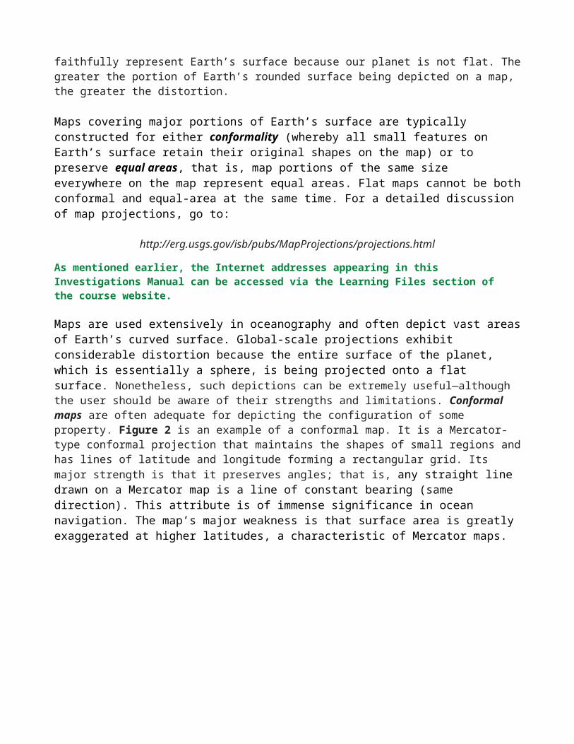
Map projections (two-dimensional representations) printed on flat sheets of paper or viewed on screens are common and convenient ways to portray features of Earth’s surface. Road maps, topographic maps, and weather maps are examples. But, like all graphical models, maps have their limitations. Over great distances, flat maps do not faithfully represent Earth’s surface because our planet is not flat. The greater the portion of Earth’s rounded surface being depicted on a map, the greater the distortion.

Maps covering major portions of Earth’s surface are typically constructed for either conformality (whereby all small features on Earth’s surface retain their original shapes on the map) or to preserve equal areas, that is, map portions of the same size everywhere on the map represent equal areas. Flat maps cannot be both conformal and equal-area at the same time. For a detailed discussion of map projections, go to:

http://erg.usgs.gov/isb/pubs/MapProjections/projections.html

As mentioned earlier, the Internet addresses appearing in this Investigations Manual can be accessed via the Learning Files section of the course website.

Maps are used extensively in oceanography and often depict vast areas of Earth’s curved surface. Global-scale projections exhibit considerable distortion because the entire surface of the planet, which is essentially a sphere, is being projected onto a flat surface. Nonetheless, such depictions can be extremely useful—although the user should be aware of their strengths and limitations. Conformal maps are often adequate for depicting the configuration of some property. Figure 2 is an example of a conformal map. It is a Mercatortype conformal projection that maintains the shapes of small regions and has lines of latitude and longitude forming a rectangular grid. Its major strength is that it preserves angles; that is, any straight line drawn on a Mercator map is a line of constant bearing (same direction). This attribute is of immense significance in ocean navigation. The map’s major weakness is that surface area is greatly exaggerated at higher latitudes, a characteristic of Mercator maps.

Figure 2. Sample Conformal Map. [Used with permission of the author, Peter H. Dana, The Geographer’s Craft Project, Department of Geography, The University of Colorado at Boulder, © 1999 Peter H. Dana]

6. Figure 2 is a Mercator flat map. An important property of such conformal maps is that lines of latitude and longitude are [(straight and perpendicular to each other)(curved)].

7. Because distortion increases away from the equator, the map in Figure 2 shows another common feature of Mercator projections, that is, the distance between adjacent lines of latitude [(decreases)(remains the same)(increases)] as latitude increases toward polar regions.

Equal-area maps portray the extent of properties while maintaining a constant scale of areas. Figure 3 is one type of equal-area world map. Equal-area maps are limited by the curvature of longitude and/or latitude lines that distorts shapes.

8. Figure 3 is an equal-area projection. Compare the apparent sizes of Greenland and South America in Figures 2 and 3. The Figure 2 Mercator map depiction suggests that they are about the same size whereas on the Figure 3 equal-area map, it is clear that Greenland is [(much larger than)(about the same size as)(much smaller than)] South America.

Figure 3. Sample Equal-Area Map. [Used with permission of the author, Peter H. Dana, The Geographer’s Craft Project, Department of Geography, The University of Colorado at Boulder, © 1999 Peter H. Dana]

Adding the Third Dimension - A Global View:

Whereas flat maps are essential and useful tools in Earth system studies, the true relations of properties and Earth locations can only be displayed on a map that approximates the real shape of our very nearly spherical planet—a globe. A globe is both conformal and equal area in its representation of Earth’s surface and its features, thereby eliminating the distortions introduced by flat map projections. It also provides an authentic representation of spatial relationships in three dimensions. This 3-D attribute is particularly useful in making models relating Earth to the Sun and Moon, investigating the effects of Earth’s rotation, and exploring the impacts of external forcings (radiational and gravitational) on the Earth system. A globe is especially useful in an ocean studies environment because it eliminates a potentially major obstacle to learning: distortion. It can be challenging to separate real patterns (or relationships) on a map from those patterns (or relationships) that appear simply because of the distortion. In other words, a globe can be a great way to put the Earth system into a more realistic perspective. (Globes are not without their limitations, however. Globes of normal size display features with relatively little detail. Another problem is that they are not as portable as flat maps!)

In this course, we utilize both flat maps and globes in our investigations of the Earth system. The Ocean Studies globe will be employed to introduce and reinforce the basic understandings of Earth system science and to provide comparisons with the more common flat-map depictions. Go 3-D: Hold your inflated Ocean Studies globe in front of you at eye level with the North Pole (coinciding with the inflation stem) pointing up. Examine the geographic coordinate grid of lines printed on the globe. These are the east-west parallels of latitude and north-south meridians of longitude. The equator (the 0-degree latitude line) is the latitude circle having the greatest circumference on this spherical globe and defines a plane that is perpendicular to Earth’s rotational axis. The equator divides Earth into two equal hemispheres, the Northern Hemisphere and the Southern

Hemisphere. A series of other east-west lines are drawn at regular north-south intervals; these are the parallels of latitude. They are labeled along the north-south 180° longitude line (in the central Pacific Ocean). Generally, latitudes in the Northern Hemisphere (equator to North Pole) are reported as degrees North (or N) or as positive (+) values, while those from the equator to South Pole are degrees South (or S) or minus (-). [On the globe, all latitudes (N or S) are marked positive.]

Because it divides Earth into two equal parts, the equator is called a great circle. A series of other great circles appears on the globe passing through the North and South Poles. These are lines of longitude and represent angular measurements around Earth in an east/west direction. They are measured from an arbitrarily chosen line termed the Prime Meridian, a longitude line (half of a great circle) running between the North and South Poles and passing through Greenwich, England. Values of longitude are printed along the equator from the Prime Meridian (0 degree longitude), increasing to the left as degrees West (or W) or to the right as degrees East (or E) until they meet in the central Pacific at 180 degrees, also called the International Date Line. [Note: Longitudes to the east of the Prime Meridian are sometimes reported positive (+) and those to the west negative (-).] The 0 degree and 180 degree longitude lines are segments of the same great circle dividing the globe into the Eastern and Western Hemispheres.

9. Any place on Earth’s surface can be specified by latitude and longitude. The deepest point on the world ocean floor is the Challenger Deep, about 11,000 m (36,100 ft) below mean sea level located at 11.3 degrees N and 142.2 degrees E in the Mariana Trench. Locate and label this place on your globe with a marking pen. It is located in the [(Indian)(North Pacific)(South Pacific)(Southern)] Ocean.

10. Locate and compare Greenland and South America on the globe. Greenland is actually [(much larger than)(about the same size as)(much smaller than)] South America. This is consistent with the depictions on the Figure 3 equal-area map.

11. Distance along a globe’s surface is the same in all directions, so distances between two locations on Earth can be easily estimated. This is possible because the distance of one longitude degree measured along the equator or one latitude degree measured along a meridian is approximately 111 km (69 statute mi). [Because these are measured along great circles, this distance is determined by dividing Earth’s circumference (about 40,000 km or 24,900 mi) by 360°.] Find the approximate distance between San Francisco, CA, and Tokyo, Japan by first determining the length of a string held taut on the globe between the two locations. Laying this length of string along the equator or a meridian would show that the number of degrees it represents is [(75)(87)(97)].

12. Multiplying the number of degrees by 111 km indicates your measurement represents a distance of about [(8,300)(9,700)(10,800)] km (5313 mi).

13. While standing and bending forward, hold your globe at about waist level and oriented so you are looking directly down on the North Pole. Note the relative amounts of land and ocean you can see. Then turn the globe over until you are looking down on the South Pole. Note the relative amounts of land and ocean seen in this view. As seen from above the two poles, the Northern Hemisphere consists of more [(water)(land)] surface than does the Southern Hemisphere. (However, both the Northern and Southern Hemispheres’ surfaces are more water than land. No matter how you look at it, Earth is a water planet!)

14. Now hold the globe at eye level. Twist and turn it until you achieve the maximum water view. The Earth looks most like a water planet when you are viewing it from in space directly over a spot on the planet’s surface at approximately at [(30 degrees S and 70 degrees E)(55 degrees N and 40 degrees E) (20 degrees S and 150 degrees W)].

Summary:

There are many reasons for studying Earth’s ocean. The AMS Ocean Paradigm describes the role of the ocean as a major component of the Earth System. The world ocean is an extremely valuable natural resource that provides food, is used for transportation and commerce, invites recreational use, and is a source of minerals and energy. It is a primary component and main driver of Earth’s climate system. Its role in climate change is especially significant because of the strong absorption of heat and carbon dioxide in seawater resulting from increased concentrations of atmospheric carbon dioxide due to the burning of fossil fuels. Exploring the ocean relies on various methods for displaying scientific information, including the use of flat-map and global map projections. The geographic coordinate system makes it possible to specify any place on Earth’s surface by latitude and longitude. Global depictions have the added value of providing authentic representation of spatial relationships in three dimensions.

EXAMPLE SUPPLEMENTAL READING ASSIGNEMNT – OCEAN RELATED CURRENT EVENTS –

Weekly Ocean NewsWEEK ONE: 5-9 September 2011

Item of Interest -

Approaching the peak in the Atlantic hurricane season -- The historic or statistical annual peak in the Atlantic hurricane season will occur this coming weekend (10-12 September), as determined as the date during the entire season with most frequent number of named tropical cyclones (tropical storms and hurricanes), based upon over 100 years of record. This date corresponds closely with the time of peak sea-surface temperatures across those sections of the North Atlantic considered hurricane-breeding areas. [NWS National Hurricane Center] [Note: So far this Atlantic hurricane season, which commenced on 1 June 2011, twelve tropical cyclones have reached tropical storm or hurricane status. Of these twelve named tropical cyclones, only two (Irene and Katia) have become hurricanes. EJH]

Ocean in the News:

Eye on the tropics --- The weather across the tropical ocean basins in the North Atlantic and the North Pacific remained active during the last week. o In the North Atlantic basin, after making landfall in the New York City metropolitan area,

Tropical Storm Irene and its remnants moved northward across sections of New England at the start of last week, producing excessive rain over the Connecticut River Valley that created major flooding in Vermont. US Geological Survey stream gauges indicated historic river levels in ten states and Puerto Rico. [USGS Newsroom] Many residents in the Middle Atlantic and New England states remained without power as of late last week due to the strong winds and heavy flooding rains that accompanied Irene. [USA Today] This tropical storm had previously been a major category 3 hurricane during the previous week as it passed across the northern Bahamas. Additional information concerning former Hurricane Irene, including satellite images and tabulation of observed rainfall totals are available on the NASA Hurricane Page. The European Space Agency (ESA) provided two interesting images from its Envisat satellite taken simultaneously of Hurricane Irene on Saturday, 27 August, soon after the hurricane had made its initial landfall along the North Carolina coast. One of the images was generated from the satellite's radar showing the rough ocean surface through the clouds, while the other image showed the typical spiral cloud pattern associated with a hurricane that was from the satellite's MERIS (MEdium Resolution Imaging Spectrometer) instrument. [ESA] At the start of last week, Tropical Storm Jose, the eleventh named tropical cyclone of the 2011 hurricane season, formed over the waters of the western North Atlantic. This tropical storm moved northward, but weakened to a tropical depression slightly more than one day after forming. Satellite images and additional information on Tropical Storm Jose appear on the NASA Hurricane Page. Early in the week, Tropical Storm Katia formed over the waters of the tropical Atlantic south of the Cape Verde Islands. Traveling to the west-northwest during the next few days, this tropical storm intensified into the second Atlantic hurricane of 2011. However, with maximum sustained wind speeds hovering between 70 and 75 mph, this minimal hurricane weakened slightly to become a tropical storm for less than a day before re-intensifying to become a hurricane late in the week. As of this past weekend, Katia continued to travel

toward the west-northwest, passing to the north of the northern Leeward Islands. The NASA Hurricane Page has satellite imagery and additional information on Hurricane Katia. A photograph of Katia, which was a tropical storm at the time, was made by astronauts on the International Space Station last Wednesday. [NASA Multimedia] Late last week, Tropical Depression 13 formed over the Gulf of Mexico and became Tropical Storm Lee. This system drifted slowly north toward the central Gulf coast last Friday and Saturday. Bands of heavy rain, along with onshore tropical storm strength winds pummeled sections of the coast throughout the weekend. Some locations had received nearly one foot of rain. By early Sunday morning, the center of Tropical Storm Lee had made landfall along the south central Louisiana coast near Lafayette, LA. [USA Today] Locally heavy rain should continue across sections of the Mid-South and Southeast through early this week as remnants of Lee follow along a projected path toward the northeast. Satellite images of Tropical Storm Lee are available on the NASA Hurricane Page.

o In the eastern North Pacific basin, Tropical Depression 8E formed over the coastal waters off southwestern Mexico at midweek. However, this depression was short-lived, when it made landfall along the coast and quickly dissipated. For more information on Tropical Depression 8E, please consult the NASA Hurricane Page.

o In the western North Pacific basin, Tropical Storm Talas continued to travel northward early in the week before curving toward the north-northwest. By late in the week, this tropical storm passed across the Japanese islands of Shikoku and Honshu on Saturday. As many as 20 people were killed as this system traveled across the island by Sunday. [USA Today] Talas was expected to lose its tropical characteristics and become an extratropical low pressure system as it travels north across the Sea of Japan on Monday (local time). The NASA Hurricane Page has additional information and satellite imagery on Tropical Storm Talas. Over this past weekend, a new tropical depression that had formed northeast of the Northern Mariana Islands became Tropical Storm Noru. This system quickly traveled to the north-northeast and remained a tropical storm late Sunday (local time).

Earthquake in Aleutians does not generate tsunami -- A magnitude 6.8 earthquake was detected during the early hours of last Friday morning southwest of Amukta Island in the Alaska's Aleutian Island chain. Upon analysis of the data, NOAA's Pacific Tsunami Warning Center did not issue a tsunami warning for the islands or other coastal locations in Alaska or western North America. [Alaska Native News]

Sea floor surveys designed to keep shipping safe off Long Island -- The 208-foot hydrographic survey vessel, NOAA Ship Thomas Jefferson, is currently conducting a three-month survey of the ocean floor off the coasts of New York, Connecticut and Rhode Island in an effort to update nautical charts for Block Island Sound. The survey project, which is managed by NOAA's Office of Coast Survey, is designed to keep large ships and commerce moving safely. [NOAA News]

Historic effort is undertaken to protect North Atlantic humpback whales -- Last week, officials from NOAA and France's Protected Areas Agency signed a "sister sanctuary" agreement designed to support the protection of endangered humpback whales that migrate annually more than 3000 miles between NOAA's Stellwagen Bank National Marine Sanctuary off the Massachusetts coast and Agoa Marine Mammal Sanctuary in the Caribbean's French Antilles. [NOAA News]

Robotic floats used to help monitor ocean acidity -- A team of researchers from the University of Washington and their Canadian colleagues have been employing a method that they developed for determining the relationships between sea water temperature, oxygen, total carbon dioxide and acidity (pH) on temperature and oxygen data collected by the fleet of ARGO submersible floats to monitor the chemistry of the world's ocean. Approximately 3000 active floats are distributed throughout the global ocean at any time. [NOAA News]

New earth-observing research satellite is being readied for launch -- During the last week, the spacecraft that represents NASA's next earth-observing research satellite arrived at California's Vandenberg Air Force Base so that preparations can begin for a launch in October. Known as the National Polar-orbiting Operational Environmental Satellite System Preparatory Project (NPP), this spacecraft represents the first of a new generation of polar-orbiting satellites that are designed to monitor changes in the atmosphere, oceans, vegetation, ice and solid Earth. [NASA's Goddard Space Flight Center]

Warmer streams could signal end for salmon -- Scientists at the University of California-Davis, the National Center for Atmospheric Research and Sweden's Stockholm Environment Institute warn that increasing temperatures in some of California's streams could signal the end of spring-run Chinook salmon in the state by the end of the century. [UC Davis News]

Methods used by bacteria to capture carbon in the ocean "twilight zone" are studied -- A team of scientists including those from the US Department of Energy's Joint Genome Institute have been studying how carbon is fixed in those sections of the oceans at depths ranging between 200 and 1000 meters below the surface called the "twilight zone." Although light is insufficient for most microorganisms, some resident microbes capture carbon dioxide that are used to form cellular structures and conduct necessary metabolic reactions. [Department of Energy Joint Genome Institute]

Changes in ice sheets and climate seen during late Pleistocene -- Researchers from the National Center for Atmospheric Research, Oregon State University, the University of Wisconsin-Madison and China's Nanjing University of Information Science and Technology have found that massive iceberg discharges into the North Atlantic Ocean during the last Ice Age were caused by changes in climate rather than ice sheet instability as previously thought. [UCAR/NCAR Staff Notes]

Dust in the Southern Hemisphere has major effect on climate during last million years --Researchers from Spain's Universitat Autònoma de Barcelona and the Swiss Federal Institute of Technology who analyzed dust and iron fluxes deposited in the Antarctic Ocean during the past 4 million years have found a close relation between the maximum contributions of dust to this ocean and climate changes occurring in the most intense glaciation periods of the Pleistocene period approximately 1.25 million years ago. Their data confirms the role of iron in the increase in phytoplankton levels during glacial periods, intensifying the function of this ocean as a sink for carbon dioxide. [Universitat Autònoma de Barcelona Latest News]

An All-Hazards Monitor --This Web portal provides the user information from NOAA on current environmental events that may pose as hazards such as tropical weather, drought, floods, marine weather, tsunamis, rip currents, Harmful Algal Blooms (HABs) and coral bleaching. [NOAAWatch]

Global and US Hazards/Climate Extremes -- A review and analysis of the global impacts of various weather-related events, to include drought, floods and storms during the current month. [NCDC]

Earthweek --Diary of the Planet [earthweek.com] Requires Adobe Acrobat Reader.

Concept of the Week: Touring the AMS Ocean Studies website

NOTE: This Concept for the Week is a repeat of that which appeared in last week's Weekly Ocean News.

Welcome to AMS Ocean Studies! You are embarking on a study of the world ocean and the role of the ocean in the Earth system. This unique teacher enhancement course focuses on the flow and transformations of energy and water into and out of the ocean, the internal properties and circulation of the ocean, interactions between the ocean and the other components of the Earth system, and the

human/societal impacts on and responses to those interactions. Throughout this learning experience, you will be using the AMS Ocean Studies website to access and interpret a variety of environmental information, including recent observational data. The objective of this initial Concept of the Week is to explore features of the AMS Ocean Studies website.

On Monday of each week of the course, we will post the current Weekly Ocean News that includes Ocean in the News (a summary listing of recent events related to the ocean), Concept of the Week (an in-depth analysis of some topic related to the ocean in the Earth system), and Historical Events (a list of past events such as tsunamis or specific advances in the understanding of oceanography). When appropriate, a feature called Supplemental Information-In Greater Depth will be provided on some topic related to the principal theme of the week.

You will use the AMS Ocean Studies website to access and download the weekly "Current Ocean Studies" (plus supporting images) that complement Investigations found in your Ocean Studies Investigations Manual. These materials should be available Monday morning. Click the appropriate links to download and print these electronic Current Ocean Studies and answer forms as well as your Investigations Response forms.

The body of the AMS Ocean Studies website provides links to the Earth System, information on Physical & Chemical, Geological, and Biological aspects of the ocean, Atmosphere/Ocean Interaction, the Great Lakes, and extras-a glossary of terms, maps, educational links, and AMS Ocean Studies information. Following each section is a link to other sites that examine the various subsystems of the Earth system. Let's take a quick tour to become more familiar with the AMS Ocean Studies website.

Under Physical & Chemical, click on Sea Surface Temperatures. This image uses a color scale to depict the global pattern of sea surface temperatures (SSTs) (in degrees Celsius) averaged over a recent 7-day period and based on measurements by infrared sensors onboard Earth-orbiting satellites. (Depending on your browser, you may have to place your mouse cursor on the slide bar to the right and scroll down to view the entire image.) Compare SSTs in the Northern Hemisphere with those in the Southern Hemisphere. Return to the AMS Ocean Studies website.

Under Geological, click on Current Earthquake Activity. The USGS Current World Seismicity page provides a global map of the locations of seismic (earthquake) events color-coded for the past seven days. The size of the squares represents the magnitude of recent earthquakes. Note how earthquakes are concentrated along the margin of the Pacific Ocean. Details of recent earthquakes can be found by clicking on their map squares. Return to the AMS Ocean Studies website.

The ocean is home to a wide variety of habitats and organisms. Under Biological, click on Ocean "Color" (Productivity). This is a satellite-derived (SeaWiFS) color-coded map of biological productivity in the surface waters of the world ocean is averaged from October 1978 to date. Orange and red indicates the highest productivity, while dark blue and violet indicate the lowest productivity. Note the vast areas of relatively low productivity over the central regions of the subtropical ocean basins. Individual months within this period may be chosen for viewing. Now return to the AMS Ocean Studies website.

Under Atmosphere/Ocean Interaction, click on TRMM Tropical Rainfall. The TRMM (Tropical Rainfall Measuring Mission) page includes color-coded maps of the Monthly Mean Rainrate (in mm per day) across the tropics for the last 30 days ending on the present date. Changes in rainfall are linked to large-scale shifts in the atmosphere/ocean circulation in the tropics. Now return to the AMS Ocean Studies website.

Take a few minutes when you have time to browse the other data and information sources available via the AMS Ocean Studies website. You should "bookmark" ("favorites") this page on your computer. Return frequently to learn more about the many resources on the ocean in the Earth system. Bon voyage!

Historical Events

5 September 1987...A tropical storm, which formed off the South Atlantic coast, was responsible for torrential rains over coastal regions of South Carolina. Between 30 August and 8 September, Charleston, SC received 18.44 in. of rain. The heavy rains caused extensive flooding around the city of Charleston, seriously damaged cotton crops in the eastern part of the state, and resulted in an unusually high number of mosquitoes. (Storm Data)

5 September 1946...The U.S. Air-Rescue Agency, an inter-departmental group headed by the Commandant of the Coast Guard and engaged on the study of improved and standardized rescue and search methods, was renamed the Search and Rescue Agency. "Search and Rescue Units" of the Coast Guard were at the same time integrated into the peace time organization and the whole developed into a system of constantly alerted communications, coastal lookout, and patrols of institute instant and systematic search and rescue procedure in case of disasters." (USCG Historian's Office)

5 September 1950...Hurricane Easy produced the greatest 24-hour rainfall in U.S. weather records up to that time. The hurricane deluged Yankeetown, on the upper west coast of Florida, with 38.70 in. of rain. This record has since been replaced by 43 in. of rain at Alvin, TX on 25-26 July 1979. (David Ludlum)

6 September 1522...The Magellan expedition completed its historical circumnavigation of the globe as one of Ferdinand Magellan's five ships, the Vittoria, arrived at Sanlýcar de Barrameda in Spain with 17 other crewmembers and four Indians. Magellan, who lost his life in April 1521 in the Philippines, set sail from Spain with 270 seamen on 20 September 1519 in an effort to find a western sea route to the rich Spice Islands of Indonesia. (The History Channel)

7 September 1934...US Coast Guard (USCG) vessels responded to a fire aboard the liner Morro Castle six miles off the New Jersey coast. This disaster, which resulted in the loss of 133 of the 455 passengers and crew, led to a Senate investigation and subsequent changes in maritime safety regulations. (USCG Historian's Office)

8 September 1900...The greatest weather disaster in U.S. records occurred when a hurricane struck Galveston, TX. Waves fifteen feet high washed over the island demolishing or carrying away buildings, and drowning more than 6000 persons. The hurricane destroyed more than 3600 houses, and total damage was more than $30 million. Winds to 120 mph, and a twenty-foot storm surge accompanied the hurricane. Following the storm, the surf was three hundred feet inland from the former water line. The hurricane claimed another 1200 lives outside of the Galveston area. (8th -9th) (David Ludlum) (The Weather Channel) Editor's note: The National Oceanic and Atmospheric Administration (NOAA) posted a webpage commemorating the Galveston, TX hurricane of 1900. This page contains links to historic photos and excerpts of an eyewitness description of storm by Isaac Cline, the chief forecaster of the Galveston U.S. Weather Bureau Office.

9 September 1945 - A "computer bug" is first identified and named by LT Grace Murray Hopper while she was on Navy active duty in 1945. It was found in the Mark II Aiken Relay Calculator at Harvard University. The operators affixed the moth to the computer log, where it still resides, with the entry: "First actual case of bug being found." They "debugged" the computer, first introducing the term. (Naval History Center)

10 September 1919...A hurricane struck the Florida Keys drowning more than 500 persons. (David Ludlum)

10 September 1965...Hurricane Betsy slammed Louisiana with wind gusting to 130 mph at Houma,

resulting in 58 deaths and over 17,500 injured. The storm surge and flooding from torrential rains made Betsy the first billion-dollar hurricane with losses exceeding $1.4 billion.

11 September 1961...Very large and slow moving Hurricane Carla made landfall near Port Lavaca, TX. Carla battered the central Texas coast with wind gusts to 175 mph, and up to 16 inches of rain, and spawned a vicious tornado (F4 on the Fujita tornado intensity scale) which swept across Galveston Island killing eight persons and destroying 200 buildings. A storm surge of up to 18.5 feet inundated coastal areas and Bay City was deluged with 17.1 inches of rain. The hurricane claimed 45 lives, and caused $300 million in damage. The remnants of Carla produced heavy rain in the Lower Missouri Valley and southern sections of the Upper Great Lakes Region. (David Ludlum) (Storm Data) (Intellicast)

11 September 1992...Hurricane Iniki, the third most damaging hurricane in US history, hit the Hawaiian Islands of Kauai and Oahu. Six people died as a result of the hurricane.

Return to AMS Ocean Studies website

Prepared by AMS Ocean Central Staff and Edward J. Hopkins, Ph.D., email hopkins@meteor.wisc.edu © Copyright, 2011, The American Meteorological Society.

EXAMPLE SUPPLEMENTAL READING

SUPPLEMENTAL INFORMATION … IN GREATER DEPTH

Week One: 5-9 September 2011

OCEAN CHARTS, UNITS, LOCATION, AND TIME

NOTE: This Supplemental Information is a repeat of that which appeared in last week's Supplemental Information…In Greater Depth file.

Ocean scientists use many different graphical representations and some units unique to the field. In this week's Supplemental Information, we describe a few examples of oceanographic charts and define some units commonly used in ocean science. Throughout our study of AMS Ocean Studies, we will encounter these, together with other charts and units. In this supplement, we also briefly explain latitude and longitude as well as time keeping, important information for navigating the high seas.

OCEAN CHARTS

A chart is a graphical model that assembles and displays data in an organized format that can be readily interpreted. Like all models, a chart is an approximation of actual conditions or the system that is represented. An oceanographic chart is a two-dimensional representation of a portion of a water body that is typically used for navigation purposes. For example, a bathymetric chart is a plot of the depth of the ocean floor (in feet, meters, or fathoms) below the datum, that is, mean sea level. Often contours are drawn connecting points of equal depth. Some U.S. government charts are color-coded with dark blue representing water 0-18 ft deep, light blue 18-36 ft, and very light blue to white more than 36 ft deep. From the contour pattern, mariners can determine the location of sea floor features (e.g., ridges, abyssal plains), the relief of the ocean bottom (the change in elevation between points), and slope or gradient (the inclination of the ocean bottom). The slope is equal to the relief divided by the horizontal distance over which the slope is measured. The closer the spacing of the contours the steeper is the slope. Other oceanographic charts plot the type of sediment or bedrock on the ocean floor. Most navigation charts include both types of data.

In the early days, water depth was determined by lowering a weighted rope or cable to the ocean floor. This line was marked off in 6-foot increments called a fathom, a unit of water depth measurement unique to ocean studies. (One fathom corresponds to 1.83 meters.) According to the Naval Historical Center, the fathom was once defined by an act of British Parliament as "the length of a man's arms around the object of his affections." The word derives from the Old English Faethm, which means "embracing arms." Today, sound waves are used to obtain much more accurate and detailed profiles of the ocean bottom. In the first Essay of Chapter 2 of your textbook, we describe the various techniques used by oceanographers to determine the depth and composition of the seafloor.

LATITUDE AND LONGITUDE

Precise location of a ship at sea is extremely important in any oceanographic enterprise, this is especially the case in the open ocean out of sight of any coastal landmarks. As with locations on land, oceanographers use the familiar latitude/longitude grid. The concept of latitude and longitude as imaginary reference lines on the globe by which location could be specified dates to the Egyptian

geographer Ptolemy about A.D. 150. As you examine your AMS Ocean Studies globe, note that lines of latitude run east-west forming circles that decrease in circumference from the equator to the poles.

Latitude describes the angular displacement that a point on the Earth's surface is with respect to the equator, while longitude is the angular displacement that the point would be from some reference meridian, usually taken as the Greenwich Prime Meridian. For centuries, angular measurements describing the geographic coordinates of latitude and longitude were expressed in sexagesimal (base-sixty) units. In this numerical system, which originated with the ancient Sumerians (ca. 2000 BC), each degree is divided into 60 minutes of arc (identified by the symbol ') and each minute is divisible by 60 seconds of arc (identified by the symbol "). Therefore, latitude is expressed in degrees where 1 degree = 60 minutes and 1 minute = 60 seconds. The equator is assigned a latitude of 0 degrees. Latitude increases north and south of the equator reaching 90 degrees N at the North Pole and 90 degrees S at the South Pole. Lines of longitude (also called meridians) run north-south and converge toward the North Pole and South Pole. By convention, the 0-degree longitude line (the prime meridian) runs through Greenwich, England. Longitude is measured in degrees west and east of the prime meridian to 180 degrees. (Again, 1 degree of longitude = 60 minutes and 1 minute = 60 seconds.)

With the development of computers and the widespread use of global positioning system (GPS) technology, geographic coordinates are expressed often in terms of degrees and decimal equivalents. Thus, the latitude of the current Tropic of Cancer, which was 23° 26' 22", could be expressed as 23.4394°. Furthermore, in many computer-generated tabulations, the designation of N and S are dropped, with latitudes of locations in the Northern Hemisphere expressed with positive (+) numbers, while Southern Hemisphere locations have negative (–) latitude values. Longitude is sometimes counted in such a way that locations in the Eastern Hemisphere have a positive value, while Western Hemisphere longitudes are negative.

On land (at least in the U.S. and some other English-speaking nations) we commonly express distances in statute miles or simply miles where 1 mile = 5280 ft = 1609.35 m. In ocean navigation, however, distance is given in nautical miles. One nautical mile is equivalent to 1 minute change in latitude at the equator = 1852 m = 6076.103 ft. At 45 degrees N or S, one degree of latitude = 59.96 nautical miles = 69.05 statute miles = 111.1 km. (The slight difference between the distance equivalents of one degree of latitude between the equator and 45 degrees N or S is caused by the oblate spheroidal shape of Earth.) One knot is a speed of one nautical mile per hour and is equivalent to 1.1516 statute miles per hour or 0.515 meters per second. Knots are commonly used as a measure of ocean current velocity, winds at sea, as well as for the speed of ships.

Prior to today's satellite-based navigation (global positioning system), mariners relied on the sun's position in the sky and other astronomical fixes to determine their latitude in the open ocean. As discussed in more detail in the first Essay of Chapter 5 in your textbook, accurate time keeping was key to determining longitude at sea.

NOAA's National Hurricane Center has an interactive "Latitude/Longitude Distance Calculator" at http://www.nhc.noaa.gov/gccalc.shtml that allows you to determine the distance between two points in nautical miles, statute miles or kilometers once you enter the latitude and longitude values of the two locations. Latitudes and longitudes may be entered in any of three different formats, decimal degrees (DD.DD), degrees and decimal minutes (DD:MM.MM) or degrees, minutes, and decimal seconds (DD:MM:SS.SS).

TIME KEEPING

Civil time zones were instituted in the U.S. and Canada in November 1883 to standardize time keeping. Prior to this, time was based on local sun time. The concept of international time zones was officially adopted in November 1884 at the International Meridian Conference in Washington, DC. Because collection and exchange of geophysical (including oceanographic) data are of international concern, use of a single worldwide time system was needed so that all observers around the world could take measurements simultaneously providing, for example, a "snapshot" of weather conditions at sea. By convention, the international system of time keeping is based on the time at the prime meridian and designated Greenwich Mean Time (GMT). This time system is based on the daily rotation of the Earth with respect to a "mean sun." Often, the single letter "Z" (phonetically pronounced "Zulu") is used because this letter identifies the Greenwich time zone. Currently, the approved practice is to use the more precise Coordinated Universal Time or Temps Universel Coordinné system (UTC), which is based on an atomic clock and time reckoned according to the stars (known as mean sidereal time). For practical purposes, GMT and UTC are equivalent.

Earth rotates on its axis with respect to the sun once every 24 hours. Hence, we should have 24 civil time zones of equal width. The 360 degrees of rotation divided by 24 give 15 degrees of width to each time zone. The central meridian of the time zone is then defined as a longitude evenly divisible by 15. If you were located in the U.S. Central Time zone where Central Standard Time (CST) is observed, you would be near 90 degrees W longitude (6 times 15). At any place within this zone, the time would be 6 hours different from the time at Greenwich, England. Earth rotates eastward so that Greenwich is ahead of CST by 6 hours. For example, when it is noon at Greenwich (1200 UTC), it is 6 a.m. in the Central Time Zone. To reduce confusion, all times should be expressed in the 24-hour format, so that 8:45 a.m. corresponds to 0845 and 1:15 p.m. corresponds to 1315. Modifications of the boundaries between time zones were made to accommodate political boundaries of some nations. In fact, some countries adhere to a local civil time that may differ by one half hour from that of the central meridian.

While most of the United States observes Daylight Saving Time during the summer (second Sunday in March to the first Sunday in November), UTC remains fixed and does not adhere to a "summer schedule." Therefore, you will have to adjust the time by one hour for summer. As an example, during the summer, residents of the U.S. Eastern Time Zone lag Greenwich time by only 4 hours, with 0800 EDT=0700 EST=1200 UTC.

THE TIME IS CURRENTLY...

Suppose that you would like to know the current time as maintained by the Master Clock at the U.S. Naval Observatory in Washington, DC. Get your clocks or watches ready and then access the current time from the Time Service Department at http://www.usno.navy.mil/USNO/time. The site http://www.time.gov/ also provides an accurate time check.

Return to AMS Ocean Studies website

Prepared by Edward J. Hopkins, Ph.D., email hopkins@meteor.wisc.edu © Copyright, 2011, The American Meteorological Society.

Sample Course Outline:

Example Spring Lecture Schedule

Week 1 Tuesday, Jan 28 Ch 1: Ocean in the Earth SystemThursday, Jan 30

Week 2 Tuesday, Feb 4 Ch 2: Ocean Basins & Plate TectonicsThursday, Feb 6

Week 3 Tuesday, Feb 11 Ch 3: Properties of SeawaterThursday, Feb 13

Week 4 Tuesday, Feb 18 Ch 4: Marine SedimentsThursday, Feb 20

Week 5 Tuesday, Feb 25 Ch 5: The Atmosphere and OceanThursday, Feb 27

Week 6 Tuesday, Mar 4 Ch 6 Ocean CurrentsThursday, Mar 6

Week 7 Tuesday, Mar 11 Exam ReviewThursday, Mar 13 In-Class Mid-Term ExamTuesday, Mar 18 Spring Break - No ClassesThursday, Mar 20 Spring Break - No Classes

Week 8 Tuesday, Mar 25 Ch 7 Ocean Waves and TidesThursday, Mar 27

Week 9 Tuesday, Apr 1 Ch 8 The Dynamic CoastThursday, Apr 3

Week 10 Tuesday, Apr 8 Ch 9 Marine EcosystemsThursday, Apr 10

Week 11 Tuesday, Apr 15 Ch 10: Ocean LifeThursday, Apr 17

Week 12 Tuesday, Apr 22 Ch 11 & 12: Ocean, Atmosphere and ClimateThursday, Apr 24

Week 13 Tuesday, Apr 29 Ch 15: Ocean Problems and PolicyThursday, May 1

Week 14 Tuesday, May 6 Exam Review