STUDY OF VENOUS WALL BEHAVIOUR FOR EARLY DIAGNOSIS OF DEEP

VEIN THROMBOSIS (DVT)

SYAHIDA BINTI ISHAK

A project report submitted in partial

fulfillment of the requirement for the award of the

Master of Electrical Engineering

Faculty of Electrical and Electronic Engineering

Universiti Tun Hussein Onn Malaysia

JULY 2015

iv

ABSTRACT

Deep Vein DVT occurs when a deep vein is partially or completely blocked by a blood

clot, most commonly in the legs. It can sometimes be difficult to recognize the

symptoms of DVT. However, the condition can be effectively treated once it been

diagnosed but too little attention has been paid to methods of early prevention of the

disease. Thus, the objective of this study is to diagnose the early stage of DVT by

studying the effects venous wall displacement to the valvular insufficiency In this

project, the experimental programme is conducted on 3 subjects with no history of DVT

to define the normal range of diameters in the deep veins of the thigh via ultrasound

image processing method. First part of the method is to come up with image processing

algorithm such as contrast enhancement and filtering to tracking the venous wall.

Second part is analysing the image to define the wall displacement. Two methods had

been approached; one using point to point method with 6.5% errors and the second is by

using image subtraction with 22.06% errors.

v

ABSTRAK

Penyakit Deep Vein Thrombosis (DVT) berlaku apabila terdapat ketulan darah yang

menghalang sepenuhnya atau sebahagian perjalanan darah pada saluran darah vena yang

ke dalam kebiasaannya di bahagian kaki. Simptom penyakit ini biasanya sukar dikesan

namun senang dirawat jika dikesan. Kajian pencegahan penyakit ini jarang dikaji di

peringkat permulaan sebelum menjadi serius. Oleh itu objektif projek ini adalah

mengkaji keadaan pesakit yang berisiko mendapatkannya berdasarkan saiz dan struktur

salur darah vena mereka. Satu kajian telah dilaksanakan ke atas 3 orang subjek yang

tidak mempunyai sejarah penyakit ini. Sampel ultrasound pada saluran vena mereka

diambil dan dikaji untuk menentukan saiz saluran darah vena menggunakan teknik

pemprosesan imej. Eksperimen ini telah dipecahkan kepada dua bahagian; bahagian

pertama untuk menjejak dinding salur darah vena menggunakan teknik peningkatan

kualiti imej dengan meningkatkan kontras dan menapis imej, manakala bahagian kedua

untuk mengukur saiz diameter salur darah vena tersebut. Dua kaedah telah dicuba untuk

mengukur saiz diameter salur darah vena; yang pertamanya dengan perbezaan sebanyak

6.5% menggunakan teknik dari titik ke titik, keduanya sebanyak 22.06 % perbezaan

dengan mencari perbezaan imej pertama dengan imej kedua dan melukis satu garis

tengah dan didapatkan jaraknya yang terdekat kepada dinding salur darah vena.

vi

CONTENTS

TITLE i

DECLARATION ii

ACKNOWLEDGEMENT iii

ABSTRACT iv

ABSTRAK v

CONTENTS vi

LIST OF TABLES viii

LIST OF FIGURES ix

CHAPTER 1 INTRODUCTION 1

1.1 Introduction 1

1.2 Problem statement 2

1.3 Aim and objectives 4

1.4 Scopes and Limitations 4

CHAPTER 2 LITERATURE REVIEW 5

2.1 Deep Vein Thrombosis 5

2.2 Vein properties and structures 7

2.3 Previous Study to Measure DVT 8

2.4 Ultrasound Image Processing Algorithm 8

2.5 Research Related To Enhance Ultrasound Image 9

vii

2.6 Vein Tracking Technique 11

CHAPTER 3 METHODOLOGY 12

3.1 Introduction 12

3.2 Ultrasound Data Acquisition 13

3.3 Image Processing Algorithm 14

3.4 Image Enhancement Algorithm 14

3.4.1 ROI-region-of-interest 15

3.4 2 RGB to Grayscale. 17

3.4.3 Contrast Enhancement 20

3.4.4 Filter 22

3.4.5 Invert Image 24

3.4.6 Change to Binary Image or segmentation 24

3.5 Define the vein displacement 25

3.5.1 Point to point method 25

3.5.6 Image Subtraction 26

CHAPTER 4 RESULT AND ANALYSIS 27

4.1 Preliminary Result 27

4.1.1 Selection of contrast enhancement technique 27

4.1.2 Selection of filtering technique 29

4.2 Enhancement of the Video/ Tracking Venous Wall 31

4.3 Experimental Programmes: Image difference and analysis 41

4.3.1 Point to point method 42

4.3.2 Image Subtraction 50

viii

CHAPTER 5 CONCLUSION 54

5.1 Conclusion 54

REEFERENCES 55

ix

LIST OF TABLES

3.1 Contrast Enhancement Functions 20

3.2 Filtering Functions 22

4.1 Conclusion table for threshold value 41

4.2 The pixel size 41

4.3 Summary of result for data 1 44

4.4 Summary of result for data 2 46

4.5 Summary of result for data 3 48

4.6 Diameter of popliteal vein using method point to point 49

4.7 Diameter of popliteal vein using method image subtract 53

x

LIST OF FIGURES

1.1 Venous Thromboembolism [1] 1

1.2 A review of ultrasound image taken at the popliteal vein. 3

2.1 Deep Vein Thrombosis at the thigh 6

2.2 Symptoms of DVT 6

3.1 Correlation between venous wall displacements to elasticity of the vein. 12

3.2 The location of popliteal vein at lower extremities. 13

3.3 Flowchart of the image enhancement algorithm. 15

3.4 Ultrasound Image before selecting the ROI 16

3.5 Ultrasound Image After Selecting the ROI 16

3.6 RGB image and the histogram graph 18

3.7 Grayscale image and the histogram graph 19

3.8 Invert image before on the left and after on the right 24

3.9 Line distribution 25

3.10 Absolute differences between two adjacent images with centre line and nearest

pixels with the centre line 26

4.1 Contrast Enhancement (Adjust Intensity Value by using Histogram Equalization

and CLAHE) 27

4.2 Invert image of contrast with Histogram Equalization and CLAHE 28

4.3 Contrast Enhancement (Adjust Intensity Value by using Gamma Correction)

29

4.4 Median Filter (MF) (Adaptive Filter) 30

4.5 Hybrid Median Filter (HMF) (Adaptive Filter) 30

4.6 Wiener filter (WF) (Adaptive filter) 30

4.7 First trial data with dimension 360 X 640 pixels. 31

xi

4.8 Crop image with smaller dimension 101 X 191 pixels. 31

4.9 Grayscale image 32

4.10 Contrast enhancement image using Contrast-limited adaptive histogram

equalization (CLAHE) 33

4.11 Filter image using Hybrid Median Filter 34

4.12 Inverted image 35

4.13 Last transformation the binary image with threshold=0.4824 36

4.14 Second trial data with dimension 1024 X 1280 pixels. 37

4.15 Image transformations for second trial data 38

4.16 Third trial data with dimension 480 X 640 pixels. 39

4.17 Image transformations for third trial data 40

4.18 Line selections for trial data 1 42

4.19 Line 1 42

4.20 Line 2 43

4.21 Line 3 43

4.22 Line selections for trial data 2 44

4.23 Line 1 45

4.24 Line 2 45

4.25 Line 3 46

4.26 Line selections for trial data 3 47

4.27 Line 1 47

4.28 Line 2 48

4.29 First data image subtraction method 50

4.30 Second data image subtraction method 51

4.31 Third data image subtraction method 52

1

CHAPTER 1

INTRODUCTION

1.1 Introduction

Deep vein Thrombosis (DVT) is one of the condition that cause venous

thromboembolism (VTE) which can bring to morbidity and mortality. DVT occurs

when a deep vein is partially or completely blocked by a blood clot, most commonly

in the legs. The clot may break off and travel to the vessels in the lung, causing a

life-threatening pulmonary embolism (PE) as shown in Figure 1.1.

Figure 1.1 Venous Thromboembolism [1].

2

Arteries bring oxygen-rich blood from the heart to the rest of your body,

whereas the veins are the blood vessels that return oxygen-poor blood back to the

heart. There are three kinds of veins. Superficial veins lie close to your skin, and the

deep veins lie in groups of muscles. Perforating veins connect the superficial veins to

the deep veins with one-way valves. Deep veins lead to the vena cava, the body's

largest vein, which runs directly to the heart.

Deep vein thrombosis (DVT) is a blood clot in one of the deep veins.

Usually, DVT occurs in the pelvis, thigh, or calf, but it can also occur less commonly

in your arm, chest, or other locations. It can sometimes be difficult to recognize the

symptoms of DVT. However, the condition can be effectively treated once it been

diagnosed but too little attention has been paid to methods of early prevention of the

disease.

Hence, this research will focus on early diagnosis of DVT. The method is by

measuring venous biomechanical properties such as blood flow velocity, venous wall

elasticity and tracking valve movement with the data obtained from ultrasound image

at the leg.

Detailed static and dynamic studies will be conducted to characterize the

properties and subsequently quantify how blood flow velocity and venous wall

elasticity affect valvular competency and ultimately leads to fatal DVT. Finally, a

new clinical model of DVT risk factors based on venous valve behaviour can be

proposed thereby constitutes an important contribution for predicting probability of

Deep Vein Thrombosis disease.

1.2 Problem Statement

Traditionally, DVT has been diagnosed by contrast venography. This technique

allows excellent visualisation of the venous system and identification of both

proximal and distal DVT. Thus, it is regarded as the reference standard for DVT

diagnosis. However, it has a number of limitations. The use of intravenous contrast

may be contraindicated by pregnancy, renal failure or known allergy; the procedure

may be technically difficult; it is expensive and requires expert interpretation, and it

is often uncomfortable for the patient. This has led to the search for cheaper, simpler,

non-invasive tests for DVT.

3

The early diagnosis of DVT is rarely been done as is often asymptomatic and

resolves without intervention; however, it can lead to local injury to the vein wall and

valves and is an important initiator of chronic venous insufficiency. It has been

noticed as DVT aging the vein become stiffer because of the clot hardening around

the wall. The estimation of age and maturity of DVTs is important for determining

the appropriate therapy. A new episode of acute DVT is treated with heparin or low-

molecular weight heparin followed by oral anticoagulant therapy. However, the

presence of a chronic thrombus in a symptomatic patient without a new acute

thrombus would suggest post-thrombotic syndrome, which does not require

anticoagulant therapy unless an acute thrombus is present [13].

In early stage of DVT, the clot is very small to be detected, therefore a

method of predicting the occurrence of deep vein thrombosis by non-invasive

measurement of biomechanics properties of venous wall need to be proposed.

Why image processing?

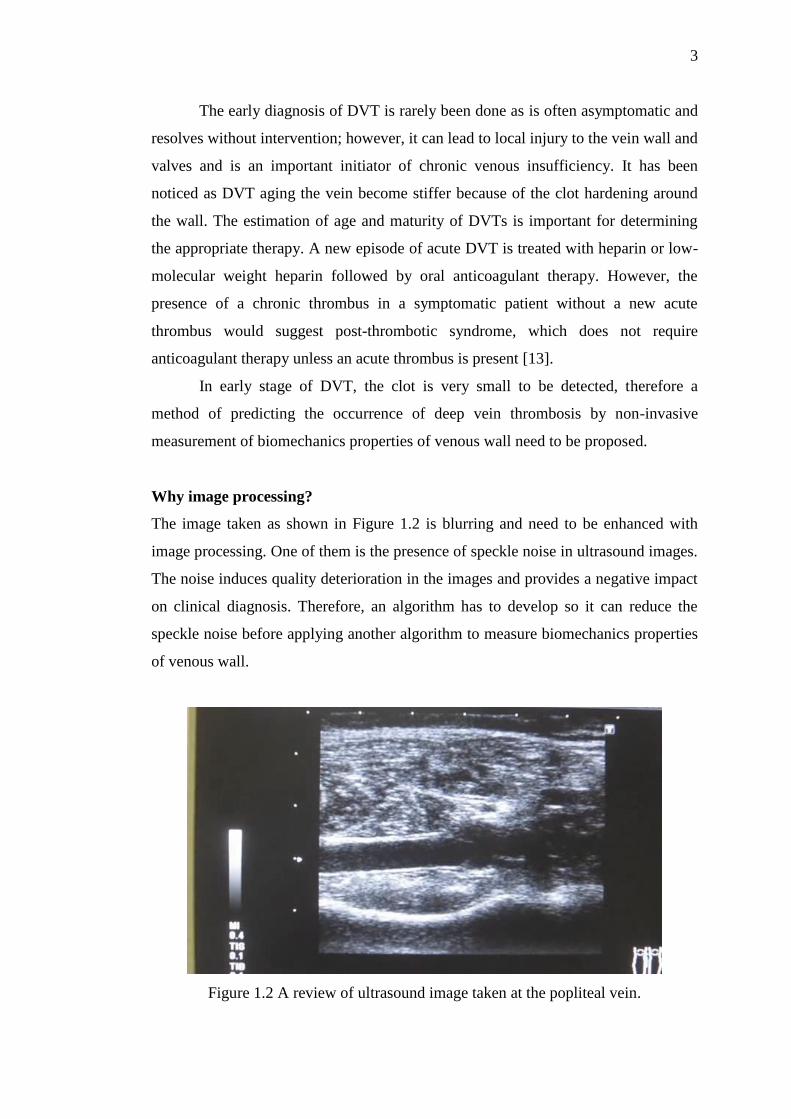
The image taken as shown in Figure 1.2 is blurring and need to be enhanced with

image processing. One of them is the presence of speckle noise in ultrasound images.

The noise induces quality deterioration in the images and provides a negative impact

on clinical diagnosis. Therefore, an algorithm has to develop so it can reduce the

speckle noise before applying another algorithm to measure biomechanics properties

of venous wall.

Figure 1.2 A review of ultrasound image taken at the popliteal vein.

4

1.3 Aim and Objectives

The research aims to study effects of blood flow velocity and venous wall

displacement to the valvular insufficiency. To achieve the aim, the following

objectives have been set:

To develop an image processing algorithm to measure the venous wall

displacement.

To evaluate the developed algorithm via a series of experiments.

To investigate the behaviour of venous wall related to the early diagnosis of

DVT in relevant conditions.

1.4 Scopes and Limitations

The scopes of this research are:

i. This research only focusses on development an image processing algorithm

to measure venous wall displacement based on ultrasound B-mode scan

image only.

ii. This study focuses on popliteal vein due to the high probability of blood clot

occurrence.

iii. In-vivo experimental studies will be conducted on controlled-subjects without

any history of DVT.

5

CHAPTER 2

LITERATURE REVIEW

2.1 Deep Vein Thrombosis

Deep vein thrombosis (DVT) is a blood clot that forms in a vein deep in the body.

Blood clots occur when blood thickens and clumps together. Most deep vein blood

clots occur in the lower leg or thigh. They also can occur in other parts of the body.

A blood clot in a deep vein can break off and travel through the bloodstream.

The loose clot is called an embolus. When the clot travels to the lungs and blocks

blood flow, the condition is called pulmonary embolism (PE). PE is a very serious

condition in which can damage the lungs and other organs in the body and

subsequently causes death. Together, DVT and PE constitute a single disease process

known as venous thromboembolism (VTE) which is an important cause of morbidity

and mortality [3].

6

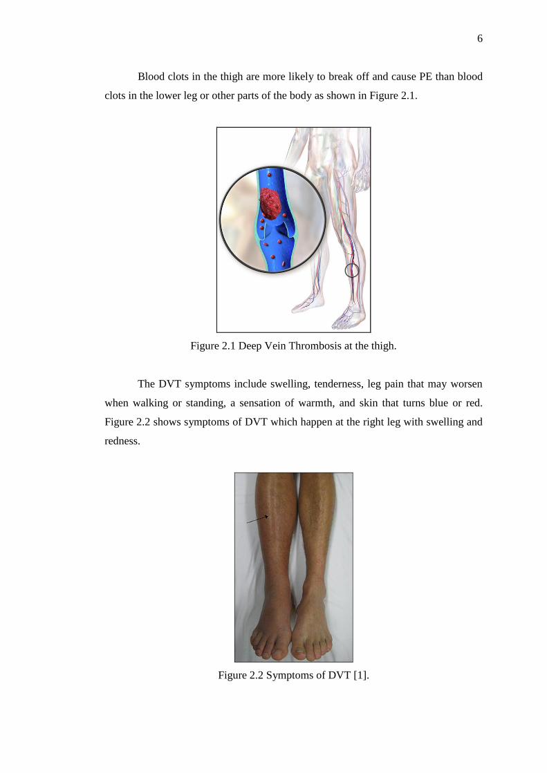
Blood clots in the thigh are more likely to break off and cause PE than blood

clots in the lower leg or other parts of the body as shown in Figure 2.1.

Figure 2.1 Deep Vein Thrombosis at the thigh.

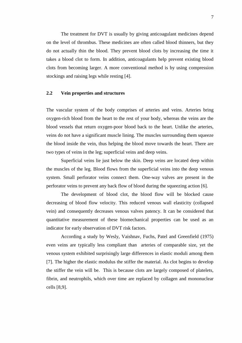
The DVT symptoms include swelling, tenderness, leg pain that may worsen

when walking or standing, a sensation of warmth, and skin that turns blue or red.

Figure 2.2 shows symptoms of DVT which happen at the right leg with swelling and

redness.

Figure 2.2 Symptoms of DVT [1].

7

The treatment for DVT is usually by giving anticoagulant medicines depend

on the level of thrombus. These medicines are often called blood thinners, but they

do not actually thin the blood. They prevent blood clots by increasing the time it

takes a blood clot to form. In addition, anticoagulants help prevent existing blood

clots from becoming larger. A more conventional method is by using compression

stockings and raising legs while resting [4].

2.2 Vein properties and structures

The vascular system of the body comprises of arteries and veins. Arteries bring

oxygen-rich blood from the heart to the rest of your body, whereas the veins are the

blood vessels that return oxygen-poor blood back to the heart. Unlike the arteries,

veins do not have a significant muscle lining. The muscles surrounding them squeeze

the blood inside the vein, thus helping the blood move towards the heart. There are

two types of veins in the leg; superficial veins and deep veins.

Superficial veins lie just below the skin. Deep veins are located deep within

the muscles of the leg. Blood flows from the superficial veins into the deep venous

system. Small perforator veins connect them. One-way valves are present in the

perforator veins to prevent any back flow of blood during the squeezing action [6].

The development of blood clot, the blood flow will be blocked cause

decreasing of blood flow velocity. This reduced venous wall elasticity (collapsed

vein) and consequently decreases venous valves patency. It can be considered that

quantitative measurement of these biomechanical properties can be used as an

indicator for early observation of DVT risk factors.

According a study by Wesly, Vaishnav, Fuchs, Patel and Greenfield (1975)

even veins are typically less compliant than arteries of comparable size, yet the

venous system exhibited surprisingly large differences in elastic moduli among them

[7]. The higher the elastic modulus the stiffer the material. As clot begins to develop

the stiffer the vein will be. This is because clots are largely composed of platelets,

fibrin, and neutrophils, which over time are replaced by collagen and mononuclear

cells [8,9].

8

2.3 Previous Study to Measure DVT

Ultrasonography combined with pulsed Doppler echocardiography (duplex imaging)

has become one of the most reliable diagnostic techniques for the evaluation of deep

vein thrombosis (DVT) of the legs. It is a combination of standard gray scale

imaging with either spectral or color Doppler and compression sonographic

scanning. The roles of gray scale and Doppler imaging are mainly just to locate the

veins. The real diagnostic portion of the test is compression sonography. Ultrasound

is widely used in elasticity imaging since motion of the speckle can be tracked over

large range of tissue deformations. When an operator pushes on tissue with a

transducer while imaging, the speckle in the image moves with the push. Tracking

the motion of the speckle permits one to determine the relative hardness of the

tissues in the image [11, 12].

Rubin et al. (2006) performed freehand compression sonographic scans using

a 5-MHz linear array transducer. Phase-sensitive B-scan frames were processed

offline by a two-dimensional complex correlation-based adaptive speckle tracking

technique. The distribution of internal strains in the wall of the vein, thrombus, and

surrounding tissue was analysed. Clot hardness was normalized to the venous wall

[13].

2.4 Ultrasound Image Processing Algorithm

According to Merriam-Webster Dictionary algorithm is a procedure that produces

the answer to a question or the solution to a problem in a finite number of steps. An

algorithm that produces a yes or no answer is called a decision procedure; one that

leads to a solution is a computation procedure. A mathematical formula and the

instructions in a computer program are examples of algorithms.

9

For ultrasound, most image processing involve algorithm as follow:

Gain Control.

This adjusts the overall brightness of the ultrasound image.

Time Gain Compensation (TGC).

TGC is used for compensating the attenuation of ultrasound echo signals along the

depth.

Dynamic Range (DR).

DR is for controlling the image contrast. Refers to the range of echoes processed and

displayed by the system, from strongest to weakest. The strongest echoes received

are those from the ‘main bang’ and transducer-skin interface and they will always be

of similar strength. As DR is reduced therefore it is the echoes at the weaker end of

the spectrum that will be lost. DR can be considered as a variable threshold of

writing for weaker signals. For general imaging the DR should be kept at its

maximum level to maximise contrast resolution potential. However in situations

where low-level noise or artefacts degrade image quality the DR can be reduced to

partially eliminate these appearances.

Edge Enhance

Edge enhancement is an image processing filter that enhances the edge contrast of an

image or video in an attempt to improve its acutance (apparent sharpness).

2.5 Research Related To Enhance Ultrasound Image

However ultrasound is still subject to a number of inherent artefacts that induces

quality deterioration in the images and provides a negative impact on clinical

diagnosis. For example, there are various sources of ‘noise’ within ultrasound images

as follow:

Speckle noise, which arises from coherent wave interference and gives a

granular appearance to an otherwise homogeneous region of tissue. Speckle

10

reduces image contrast and detail resolution, and makes it difficult to identify

abnormal tissue patterns (or texture) that may indicate disease.

Clutter noise, which arises from beam forming artifacts, reverberations,and

other acoustic phenomena. Clutter consists of spurious echoes which can

often be seen within structures of low echogenicity, such as a cyst, or within

amniotic fluid, and which may be confused with ‘real’ targets.

Thermal noise especially in deep-lying regions, arising in the electronics of

the transducer or beamformer.

Duhgoon et al. (2006) propose an algorithm to find the optimized parameter

values for Time Gain Composition (TGC) and Dynamic Range (DR) automatically

[14].In TGC optimization, they determine the degree of attenuation compensation

along the depth by reliably estimating the attenuation characteristic of ultrasound

signals. For DR optimization, they define a novel cost function by properly using the

characteristics of ultrasound images. Experimental results are obtained by applying

the proposed algorithm to a real ultrasound (US) imaging system. The results prove

that the proposed algorithm automatically sets values of TGC and DR in real-time so

that the subjective quality of the enhanced ultrasound images may become good

enough for efficient and accurate diagnosis.

Bamber et al. (1986) developed a speckle reduction algorithm that changed

the amount of smoothing depending on the local statistics of the image (the ratio of

local variance to local mean), utilizing the fact that speckle has characteristic

statistical properties and can thus be identified by its gray level distribution [15].

Where speckle is identified, the smoothing is increased; in other non-speckle regions

the smoothing is reduced or eliminated, thus preserving detail. Although preliminary

clinical evaluations on static images were encouraging, the processing time of six

seconds per frame made it unsuitable for real-time evaluation.

Loupas et al. (1994) developed a similar algorithm based on the statistical

properties of gray levels, but instead of explicitly identifying speckle the algorithm

used a generalized noise model to identify regions in which local variation of the

gray level distribution was consistent with noise (these were smoothed) or structure

(little or no smoothing) [16].

11

Stetson et al. (1997) developed an adaptive gray-scale mapping algorithm for

improving tissue contrast, although the real-time version was not continuously (i.e.

temporally) adaptive since the gray-level transforms were pre-set using static images

of similar targets [17]. There are versions of related gray-level optimization

algorithms on commercial ultrasound systems that similarly pre-set the transforms

using static images, typically acquired when the user hits an ‘optimize’ button.

2.6 Vein Tracking Technique

One of the methods to track the vein is by speckle tracking technique based on the

observation that ultrasound images contain many small particles, natural acoustic

markers, which move together with the tissue and can be identified on adjacent

frames. These natural markers are stable acoustic speckles, equally distributed within

the area. Each marker can be identified and followed accurately during several

consecutive frames. The new marker location on sequential images is tracked and the

local tissue velocity can be calculated as a marker’s shift divided by the time

between 2 consecutive frames. Changes of the distance between neighbouring

elements reflect the tissue’s contraction or relaxation.

12

CHAPTER 3

METHODOLOGY

3.1 Introduction

This chapter will introduce the method to develop an image processing and analysis

algorithm to measure venous wall displacement. Changes of the distance or

displacement between adjacent walls reflect the tissue’s contraction or relaxation and

subsequently reflect the elasticity of the vein. The correlation is simplified as Figure

3.1.

Figure 3.1 Correlation between venous wall displacements to elasticity of the vein.

The significance displacement or difference between the adjacent walls will

be analysed frame by frame. The hypothesis is as when thrombi start to deform

around the venous wall, it will affect the displacement or diameter and elasticity of

the vein as the vein become stiffer. When grouped veins with acute DVT were larger

Elasticity Displacement

Tissue’s

contraction and

relaxation

13

than normal veins. Likewise, veins with chronic DVT were smaller than normal

veins [19].

3.2 Ultrasound Data Acquisition

The trial data will be taken from a normal subject with no sign of DVT symptoms at

all. Scans were performed with standard B-mode ultrasound in the sagittal plane. The

scans area is around the thigh.

Compare to sonographic elastic imaging the method is to apply ultrasound in

B-mode without any compression to the vein. The focus will be on the venous wall

near to the valve which is called as popliteal vein as depicted by Figure 3.2.

Figure 3.2 The location of popliteal vein at lower extremities [1].

14

3.3 Image Processing Algorithm

The method will be divided into two parts;

Part 1: Image or video enhancement to tracking the venous wall compare to

other elements such as noise and blood flow. Image enhancement techniques

bring out the detail in an image that is obscured or highlight certain features of

interest in an image such as contrast adjustment and filtering, typically return a

modified version of the original image. These techniques are frequently used as

a preprocessing step to improve the results of image analysis.

Part 2: Define the wall displacement. Once the image is clear with two parts

separated which define the venous wall, the measurement between two line

takes place and will be compared from frame to frame.

3.4 Image Enhancement Algorithm

All implementations of image enhancement algorithm and analysis carried out using

MATLAB (MathWorks, R2013a) with portions of the algorithm written in the C

language to speed up the process. The analyses were performed on a personal

computer with a Intel (R) Core (TM) i7-3520M CPU running at 2.90 GHz. The PC

was running the 64-bit version of Windows 7 Professional.

Figure 3.3 shows the general flowchart of the algorithm.

15

Select Region of Interest

(ROI)

Change to Greyscale

Image

Image Contrast

Enhancement

Filter Image

Invert the Image

Segmentation or Change

to binary image

Figure 3.3 Flowchart of the image enhancement algorithm.

3.4.1 ROI-region-of-interest

An image may be considered to contain sub-images sometimes referred to as

regions–of–interest, ROIs, or simply regions. This concept reflects the fact that

images frequently contain collections of objects each of which can be the basis for a

region. In a sophisticated image processing system it should be possible to apply

specific image processing operations to selected regions. Thus one part of an image

(region) might be processed to suppress motion blur while another part might be

processed to improve color rendition [21].

16

Figure 3.4 Ultrasound Image Before selecting the ROI

Figure 3.5 Ultrasound image After Selecting the ROI

The selection is as closer to the valve and as nearest to the venous wall as

shown in Figure 3.4 and 3.5. Base on the image the tissue muscle is brighter compare

to liquid blood.

3.4.2 RGB to Grayscale

The ultrasound image is a 3D image contain RGB colour. For further analysis the

image need to be converted to 1D which is in grayscale then convert to binary image.

A grayscale image contain element from 0 to 255 while a binary image is the image

where the element is 1 and 0 only. But before converting to binary image, usually the

image need to undergo a few steps in grayscale form first so not all the information is

loss.

17

I = rgb2gray(RGB) converts the true colour image RGB to the grayscale

intensity image I. rgb2gray converts RGB images to grayscale by eliminating the

hue and saturation information while retaining the luminance and by forming a

weighted sum of the R, G, and B components:

0.2989 + 0.5870 * G + 0.1140 * B

Truecolor RGB (Figure 3.6). A truecolor red-green-blue (RGB) image is

represented as a three-dimensional M×N×3 double matrix. Each pixel has red,

green, blue components along the third dimension with values in [0,1].

Grayscale (Figure 3.7). A grayscale image M pixels tall and N pixels wide is

represented as a matrix of double datatype of size M×N. Element values (e.g.,

MyImage(m,n)) denote the pixel grayscale intensities from 0 to 255 [21].

18

Figure 3.6 RGB image

19

Figure 3.7 Grayscale image

20

3.4.3 Contrast Enhancement

Contrast enhancement changing the pixels intensity of the input image to utilize

maximum possible bins. In other words is a transformation of a sensory

representation that results in an output representation in which regions of transition

(e.g. “edges”) are selectively emphasized. The mechanisms mediating contrast

enhancement in different systems are diverse, depending critically on the breadth of

the contrast enhancement function as well as on the modality of the representation.

One can find a vast range of enhancement techniques in the literature but below is

what available in Matlab.

Table 3.1 Contrast Enhancement Functions [21].

imadjust Adjust image intensity values or colormap

imcontrast Adjust Contrast tool

imsharpen Sharpen image using unsharp masking

histeq Enhance contrast using histogram equalization

adapthisteq Contrast-limited adaptive histogram equalization (CLAHE)

imhistmatch

Adjust histogram of image to match N-bin histogram of

reference image

decorrstretch Apply decorrelation stretch to multichannel image

stretchlim Find limits to contrast stretch image

intlut Convert integer values using lookup table

imnoise Add noise to image

Three techniques have been test to enhance the contrast of the image.

Technique 1: Histogram Equalization

histeq performs histogram equalization. It enhances the contrast of images by

transforming the values in an intensity image so that the histogram of the output

image approximately matches a specified histogram (uniform distribution by default)

[21].

21

Technique 2: Contrast-limited adaptive histogram equalization (CLAHE)

CLAHE operates on small regions in the image, called tiles, rather than the entire

image. Each tile's contrast is enhanced, so that the histogram of the output region

approximately matches the histogram specified by the 'Distribution' parameter. The

neighbouring tiles are then combined using bilinear interpolation to eliminate

artificially induced boundaries. The contrast, especially in homogeneous areas, can

be limited to avoid amplifying any noise that might be present in the image.

adapthisteq performs contrast-limited adaptive histogram

equalization(CLAHE). Unlike histeq, it operates on small data regions (tiles) rather

than the entire image. Each tile's contrast is enhanced so that the histogram of each

output region approximately matches the specified histogram (uniform distribution

by default). The contrast enhancement can be limited in order to avoid amplifying

the noise which might be present in the image [21].

Technique 3: Gamma Correction

Gamma can be any value between 0 and infinity. If gamma is 1 (the default), the

mapping is linear. If gamma is less than 1, the mapping is weighted toward higher

(brighter) output values. If gamma is greater than 1, the mapping is weighted toward

lower (darker) output values.

imadjust maps low to bottom, and high to top. By default, the values

between low and high are mapped linearly to values between bottom and top. For

example, the value halfway between low and high corresponds to the value halfway

between bottom and top.

imadjust also can accept an additional argument that specifies the gamma

correction factor. Depending on the value of gamma, the mapping between values in

the input and output images might be nonlinear. For example, the value halfway

between low and high might map to a value either greater than or less than the value

halfway between bottom and top [21].

22

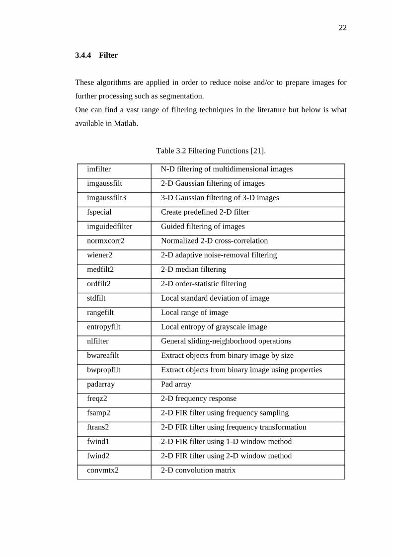
3.4.4 Filter

These algorithms are applied in order to reduce noise and/or to prepare images for

further processing such as segmentation.

One can find a vast range of filtering techniques in the literature but below is what

available in Matlab.

Table 3.2 Filtering Functions [21].

imfilter N-D filtering of multidimensional images

imgaussfilt 2-D Gaussian filtering of images

imgaussfilt3 3-D Gaussian filtering of 3-D images

fspecial Create predefined 2-D filter

imguidedfilter Guided filtering of images

normxcorr2 Normalized 2-D cross-correlation

wiener2 2-D adaptive noise-removal filtering

medfilt2 2-D median filtering

ordfilt2 2-D order-statistic filtering

stdfilt Local standard deviation of image

rangefilt Local range of image

entropyfilt Local entropy of grayscale image

nlfilter General sliding-neighborhood operations

bwareafilt Extract objects from binary image by size

bwpropfilt Extract objects from binary image using properties

padarray Pad array

freqz2 2-D frequency response

fsamp2 2-D FIR filter using frequency sampling

ftrans2 2-D FIR filter using frequency transformation

fwind1 2-D FIR filter using 1-D window method

fwind2 2-D FIR filter using 2-D window method

convmtx2 2-D convolution matrix

23

Three techniques have been test to filtering the image.

Technique 1: Median Filtering

Median filtering is similar to using an averaging filter, in that each output pixel is set

to an average of the pixel values in the neighbourhood of the corresponding input

pixel. However, with median filtering, the value of an output pixel is determined by

the median of the neighbourhood pixels, rather than the mean. The median is much

less sensitive than the mean to extreme values (called outliers). Median filtering is

therefore better able to remove these outliers without reducing the sharpness of the

image [21].

Technique 2: Hybrid Median Filtering

B = HMF (A, N) performs hybrid median filtering of the matrix A using a NxN box.

Hybrid median filtering preserves edges better than a NxN square kernel-based

median filter because data from different spatial directions are ranked separately.

Three median values are calculated in the NxN box: MR is the median of horizontal

and vertical R pixels, and MD is the median of diagonal D pixels. The filtered value

is the median of the two median values and the central pixel C: median

([MR,MD,C]) [21].

Technique 3: Wiener Filter

Wiener filters (a type of linear filter) to an image adaptively, tailoring itself to the

local image variance. Where the variance is large, it performs little smoothing.

Where the variance is small, it performs more smoothing. This approach often

produces better results than linear filtering. The adaptive filter is more selective than

a comparable linear filter, preserving edges and other high-frequency parts of an

image. In addition, there are no design tasks; the wiener filter function handles all

preliminary computations and implements the filter for an input image. However, it

does require more computation time than linear filtering. It works best when the

noise is constant-power ("white") additive noise, such as Gaussian noise [21].

24

3.4.5 Invert Image

The Invert command inverts all the pixel colours and brightness values in the current

layer, as if the image were converted into a negative. Dark areas become bright and

bright areas become dark. It is crucial since qualitatively it is easier to distinguish

vein with two separated line instead of dark images in the middle.

Figure 3.8 Invert image before on the left and after on the right

3.4.6 Change to Binary Image or segmentation

A binary image is represented by an M×N logical matrix where pixel values are 1

(true) white or 0 (false) black.

The graythresh function uses Otsu's method, which chooses the threshold to

minimize the intraclass variance of the black and white pixels.

level = graythresh(I) computes a global threshold (level) that can be

used to convert an intensity image to a binary image with im2bw. level is a

normalized intensity value that lies in the range [0, 1].

Multidimensional arrays are converted automatically to 2-D arrays using

reshape. The graythresh function ignores any nonzero imaginary part of I.

BW = im2bw(I, level) converts the grayscale image I to a binary image.

The output image BW replaces all pixels in the input image with luminance greater

than level with the value 1 (white) and replaces all other pixels with the value 0

(black). Specify level in the range [0,1]. This range is relative to the signal levels

possible for the image's class. Therefore, a level value of 0.5 is midway between

black and white, regardless of class [21].

55

REFERENCES

[1] Med India. (2013), Pulmonary Embolism and Deep Vein Thrombosis/Venous

Thromboembolism. Health Information.

[2] A. T. F. Members, et al., "Guidelines on the diagnosis and management of

acute pulmonary embolism: The Task Force for the Diagnosis and Management

of Acute Pulmonary Embolism of the European Society of Cardiology (ESC),"

European Heart Journal, vol. 29, pp. 2276-2315, September 1, 2008 2008.

[3] Hirsh J, Hoak J. Management of deep venous thrombosis and pulmonary

embolism: a statement for healthcare professionals. Council on Thrombosis (in

consultation with the Council of Cardiovascular Radiology), American Heart

Association. Circulation 1996; 93:2212–2245.

[4] Wakefield TW. Treatment options for venous thrombosis. J Vasc Surg 2000;

31:613–620.

[5] Anatomy books

[6] R L Wesly, R N Vaishnav, J C Fuchs, D J Patel and J C Greenfield, Jr. Static

linear and nonlinear elastic properties of normal and arterialized venous tissue

in dog and man. Circ Res. 1975;37:509-520

[7] Wakefield TW, Linn MJ, Henke PK, et al. Neovascularization during venous

thrombosis organization:a preliminary study. J Vasc Surg 1999;30:885–892.

[8] Henke PK, Wakefield TW, Kadell AM, et al. Interleukin-administration

enhances venous thrombosis resolution in a rat model. J Surg Res 2001; 99:84–

91.

[9] M. A. Lubinski, S. Y. Emelianov, K. R. Raghavan, A. E. Yagle,A. R.

Skovoroda, and M. O’Donnell, “Lateral displacement estimation using tissue

incompressibility,” IEEE Transactions on Ultrasonics, Ferroelectrics, and

Frequency Control, vol. 43, no. 2,pp. 247–256, 1996.

56

[10] X. Chen, M. J. Zohdy, S. Y. Emelianov, and M. O’Donnell,“Lateral speckle

tracking using synthetic lateral phase,” IEEE Transactions on Ultrasonics,

Ferroelectrics, and Frequency Control,vol. 51, no. 5, pp. 540–550, 2004.

[11] Ophir J, Cespedes I, Garra B, Ponnekanti H, Maklad N.Elastography:

ultrasonic imaging of tissue strain and elastic modulus in vivo. Eur J

Ultrasound 1996; 3: 49–70.

[12] Gao L, Parker KJ, Lerner RM, Levinson SF. Imaging of the elastic properties

of tissue: a review. Ultrasound Med Biol 1996; 22:959–977.

[13] Rubin JM, Hua Xie, Kang Kim, Weitzel WF, Emilianov SY,Alygmov SR,

Wakefield TW. Sonographic elasticity imaging of acute and chronic deep

venous thrombosis in humans. J Ultrasound Med 2006; 25:1179–1186.

[14] Duhgoon Lee, Yong Sun Kim, and Jong Beom Ra. Automatic time gain

compensation and dynamic range control in ultrasound imaging systems.

Medical Imaging 2006: Ultrasonic Imaging and Signal Processing. Proc. of

SPIE Vol. 6147.

[15] Bamber J, Daft C. Adaptive Filtering for Reduction of Speckle in Ultrasonic

Pulse-Echo Images. Ultrasonics 1986; 24: 41–44.

[16] Loupas T, McDicken N, Anderson T, Allan P. Development of an Advanced

Digital Image Processor for Real-Time Speckle Suppression in Routine

Ultrasound Scanning. Ultrasound Med Bio 1994; 20 (3): 239–249.

[17] Stetson P, Sommer F, Macovski A. Lesion Contrast Enhancement in Medical

Ultrasound Imaging. IEEE Transactions Medical Imaging 1997; 16 (4): 416–

425.

[18] Russ, J.C., The Image Processing Handbook. Second ed. 1995, Boca

Raton,Florida: CRC Press.

[19] Hertzberg B.S,Kliemer M.A.,Sonographic Assessment of Lower Limb Vein

Diameters: Implications for The Diagnosis and Characterization;AJR:168,May

1997.

[20] H. Sharifian* and F. Gharekhanloo. Evaluation of Average Diameter of Lower

Extremity Veins in Acute and Chronic Thrombosis and Comparison with

Normal Persons by Doppler. Acta Medica Iranica, 41 (3): 180-182; 2003

[21] MATLAB PDF Documentation