RESEARCH ARTICLE

Switch or stay? Automatic classification of internal mental statesin bistable perception

Susmita Sen1 • Syed Naser Daimi1 • Katsumi Watanabe2 • Kohske Takahashi3 • Joydeep Bhattacharya4 •

Goutam Saha1

Received: 14 January 2019 / Revised: 4 June 2019 / Accepted: 6 July 2019� The Author(s) 2019

AbstractThe human brain goes through numerous cognitive states, most of these being hidden or implicit while performing a task,

and understanding them is of great practical importance. However, identifying internal mental states is quite challenging as

these states are difficult to label, usually short-lived, and generally, overlap with other tasks. One such problem pertains to

bistable perception, which we consider to consist of two internal mental states, namely, transition and maintenance. The

transition state is short-lived and represents a change in perception while the maintenance state is comparatively longer and

represents a stable perception. In this study, we proposed a novel approach for characterizing the duration of transition and

maintenance states and classified them from the neuromagnetic brain responses. Participants were presented with various

types of ambiguous visual stimuli on which they indicated the moments of perceptual switches, while their magnetoen-

cephalogram (MEG) data were recorded. We extracted different spatio-temporal features based on wavelet transform, and

classified transition and maintenance states on a trial-by-trial basis. We obtained a classification accuracy of 79.58% and

78.40% using SVM and ANN classifiers, respectively. Next, we investigated the temporal fluctuations of these internal

mental representations as captured by our classifier model and found that the accuracy showed a decreasing trend as the

maintenance state was moved towards the next transition state. Further, to identify the neural sources corresponding to

these internal mental states, we performed source analysis on MEG signals. We observed the involvement of sources from

the parietal lobe, occipital lobe, and cerebellum in distinguishing transition and maintenance states. Cross-conditional

classification analysis established generalization potential of wavelet features. Altogether, this study presents an automatic

classification of endogenous mental states involved in bistable perception by establishing brain-behavior relationships at

the single-trial level.

Keywords Internal mental states � Bistable perception � MEG � Single-trial classification � Source reconstruction �SVM � ANN

& Syed Naser Daimi

sndaimi123@gmail.com

Susmita Sen

susmitasen@ece.iitkgp.ernet.in

Katsumi Watanabe

kw@fennel.rcast.u-tokyo.ac.jp

Joydeep Bhattacharya

j.bhattacharya@gold.ac.uk

Goutam Saha

gsaha@ece.iitkgp.ernet.in

1 Department of Electronics and Electrical Communication

Engineering, Indian Institute of Technology Kharagpur,

Kharagpur 721 302, India

2 Department of Intermediate Art and Science, Waseda

University, Tokyo, Japan

3 School of Psychology, Chukyo University, Nagoya, Japan

4 Department of Psychology, Goldsmiths, University of

London, London, UK

123

Cognitive Neurodynamicshttps://doi.org/10.1007/s11571-019-09548-7(0123456789().,-volV)(0123456789().,- volV)

Introduction

The human brain has a unique ability to perform various

cognitive processes that can be represented by different and

potentially distinct cognitive states. In the last decade, there

has been intense interest in exploring the possibility to

decode underlying cognitive states from the observed brain

signals measured by neuroimaging techniques (Haynes and

Rees 2006; Richmond et al. 2012). For example, studies

performed decoding of mental states underlying resting

state, recalling events, performing mathematical computa-

tion and singing (Shirer et al. 2012), decoding of speech or

video quality perception (Porbadnigk et al. 2013; Acqua-

lagna et al. 2015), detecting the level of alertness (Hsu and

Jung 2017) from their ongoing brain activity. Under-

standing and identifying the mental states through brain

responses can be of great importance in human-machine

interaction and brain-computer interfaces (BCI) applica-

tions (Calvo et al. 2014). Most studies deal with decoding

the perception of objects and visual images, namely

decoding the perceptual states while visualizing face or any

objects (Allison et al. 1994; Kanwisher et al. 1997), house

or visual scenes (Epstein and Kanwisher 1998), as well as

orientation, location, color, and direction of motion of

objects (Carlson et al. 2011; Haynes and Rees 2005;

Kamitani and Tong 2005). These processes are dependent

upon the information contained in the visual stimuli.

Further, decoding of spontaneously changing dynamical

states, that come close to the practical scenario is also

studied (Haynes and Rees 2006). Such stimuli include

ambiguous visual stimuli, e.g., binocular rivalry or

bistable figures (Fig. 1), which can be perceived with two

interpretations but without any concomitant change in the

external sensory input. Hence, there is a sharp dissociation

between consistent visual stimuli and fluctuating conscious

awareness (Blake and Logothetis 2002). In this study, we

considered the problem of decoding the internal mental

states involved with bistable perception.

The studies that use bistable stimuli, mostly analyze the

brain responses of the alternating states of the perception

(Knapen et al. 2011; Sterzer et al. 2009; Isoglu-Alkac et al.

2000). Among these studies, a large number uses fMRI

data (Knapen et al. 2011; Sterzer et al. 2009), but there are

also a few studies using EEG/MEG. For example, Isoglu-

Alkac et al. (2000) have experimented with Necker cube as

visual stimuli and have compared the alpha band

(8–16 Hz) activity in two-time windows: 800–440 ms and

440–80 ms before the button press at perceptual change.

They have found a noticeable decrease in alpha activity

from former time window to the latter one. Interestingly,

another study (Isoglu-Alkac and Struber 2006) reported a

decrease in only the lower alpha band (6–10 Hz) power,

while the upper alpha band (10–12 Hz) activity remained

unchanged. The MEG alpha band activities during the

perceptual reversal in case of exogenously and endoge-

nously induced reversal were also compared (Struber and

Herrmann 2002). Endogenous reversal of perceived motion

direction takes place spontaneously in the presence of

constant ambiguous stimuli, whereas, exogenous reversals

are driven by a change in external stimuli. In both cases,

participants were instructed to press a button whenever a

change in the perceived motion direction occurred. The

authors have reported that in the case of an exogenously

induced reversal, alpha activity (10 Hz) started decreasing

between 300 and 200 ms before the button press. On the

contrary, in the case of an endogenously induced reversal,

alpha activity decreased within 1000 ms before the button

press. In another study (Basar-Eroglu et al. 1996), it is

observed that high-frequency gamma band (30–50 Hz)

oscillations were dominant in the right frontal cortex within

1000 ms before the button press. Recently, Kloosterman

et al. (2015) studied motion-induced blindness, another

perceptual illusion under identical sensory input, and

reported that this illusion was associated with the beta

band (12–30 Hz) oscillations over visual cortex out of top-

down modulation.

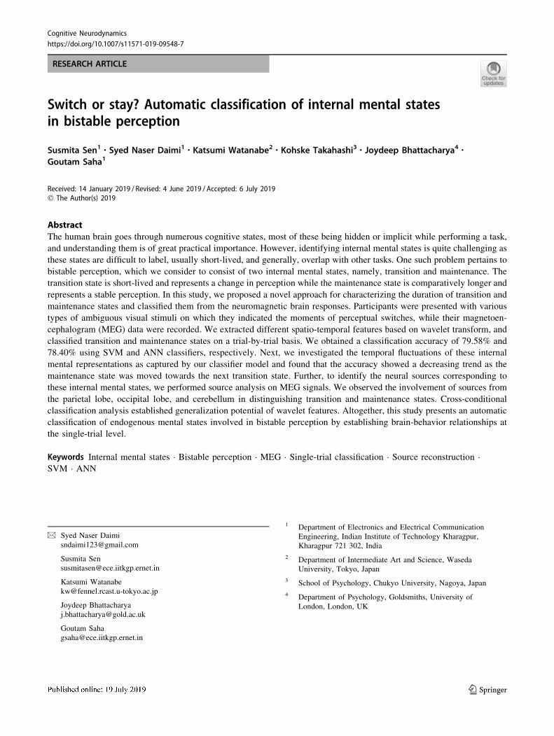
Fig. 1 Bistable visual stimuli used in this experiment. a Necker Cube

(NC): front surface flips with time; b structure-from-motion (SFM):

sphere made of dots seems to move in anticlockwise or clockwise

direction; c stroboscopic alternative motion (SAM): frame1 and

frame2 are presented in such a manner that there lies an ambiguity in

the direction in which dots move—horizontally or vertically

Cognitive Neurodynamics

123

These studies suggest that the large scale brain oscilla-

tions and their temporal dynamics are associated with

perceptual switching bistable perception. This further

suggests that the underlying cognitive states are dynamic.

In bistable perception, the subjective perception alternates

between two interpretations spontaneously and without any

change in the visual input; besides two perceptual states,

the processing itself contains separate internal mental

states—transition and maintenance (Rees 2001). During

the state of transition, perception switches from one per-

ception to another. On the other hand, one perception

remains unaltered throughout the maintenance state. The

earlier studies on bistable perception, albeit informative

and explanatory towards revealing the neuronal mecha-

nisms underlying ambiguous visual perception, has so far

not aimed to classify internal mental states, transition and

maintenance, on a single-trial basis. The task of distin-

guishing these states through brain signals is not trivial as

the underlying processes for bistable perception overlap

with those of simple perception (Long and Toppino 2004),

the rapid occurrence of transition further makes it difficult

to analyze on a single-trial basis. The principal aim of this

study was to classify the internal mental states of the brain

that goes through the states of transition and maintenance

around the moment of the perceptual switch during

bistable visual perception on a single-trial basis.

The neuromagnetic brain responses (MEG) were recor-

ded from eleven healthy participants while they were pre-

sented with ambiguous bistable visual stimuli. We used a

machine-learning framework involving feature extraction,

dimensionality reduction, and classification. The complex

Morlet wavelet transform was used to extract spectral

features that capture the spatiotemporal dynamics of large-

scale brain oscillations. Three types of features were pro-

posed that capture the spatiotemporal brain activity at

different spatial scales—overall (global), hemispheric, and

regional (local) brain activity, respectively. For dimension

reduction, we followed the Principal Component Analysis

(PCA) based approach. Finally, we validated our classifi-

cation performance using two widely used classifiers,

namely Support Vector Machine (SVM) and Artificial

Neural Network (ANN).

This study addresses several challenges associated with

decoding the internal mental states involved in

bistable perception. Our contributions are as follows.

1. The internal mental states changes spontaneously, that,

are not locked to a trigger in external stimuli. This

makes labelling them difficult. Here, we considered the

MEG signal before and after the button press to define

the transition and maintenance state. The reason is that

the participants were instructed to report the perceptual

switch while they were viewing bistable stimuli. It is

likely that the change in perception had occurred a

little ahead of the time the perceptual switches were

reported.

2. The transition state is short-lived as compared to

maintenance state. It is of interest to determine the

shortest duration of the transition state, that distin-

guishes it from the maintenance state. For this purpose,

we adopted the machine learning framework to infer an

effective duration of the transition state.

3. We investigated if the underlying states, as captured by

the decoding performance, differed across the type of

bistable stimuli considered. For this, we used three

types of bistable stimuli (Fig. 1): Necker cube (NC),

apparent motion or stroboscopic alternative motion

(SAM) and structure-from-motion (SFM).

4. We propose a framework to characterize the variation

of the maintenance state with time. As mentioned

earlier, the maintenance state extends over a longer

duration than the transition state. Here, we investigated

if the underlying neural representation remains

stable over the maintenance period; the proposed

framework captures the intrinsic temporal fluctuations

of maintenance state representation, in terms of its

decoding performance.

5. We localized the underlying brain sources whose

activity is modulated by the internal mental state under

consideration.

6. We investigated the neural abstraction in discriminat-

ing transition and maintenance states across different

stimulus types, that is, whether the brain responses

captured by wavelet features are generalized across

different stimulus types. For this, we utilized cross-

conditional classification approach where data of one

stimulus type was used for training and testing it with

the data from other stimulus types.

Altogether, this work designed and presented a direction to

characterize and decode internal mental states involved in

bistable perception at the single-trial level.

Materials and methods

Dataset

Participants

In this experiment, MEG data were recorded from eleven

adult participants. All participants were right-handed,

neurologically healthy and had normal vision. Written

informed consent was obtained from all participants. The

experimental protocol was approved by the Local Ethics

Committee and followed the declaration of Helsinki.

Cognitive Neurodynamics

123

Stimuli

Three types of bistable stimuli were used, namely: Necker

cube (NC), apparent motion or stroboscopic alternative

motion (SAM) and structure-from-motion (SFM) (Fig. 1).

The perceptual interpretation of Necker cube oscillates

between two different recessional surfaces. In the case of

SAM, there is an ambiguity about the direction in which

the dots move—horizontally or vertically. The SFM used

here was a sphere comprised of dots that seems to be

moving. While observing SFM, the perceived direction of

rotation appears to flip over time.

Procedure

Visual stimuli were projected onto a rear screen, located 32

cm from the participant’s eyes by a projector (PG-B10S;

SHARP, Osaka, Japan) via a mirror. The visual stimuli

were generated by using C?? and OpenGL. The size and

luminance were far above visual threshold. The rotating

sphere consisted of 200 dots. The basic experimental set-

ting was identical with a previously published article

(Kondo et al. 2010). There were 18 trials (3 [stimulus

type] 9 2 [stimuli presentation type] 9 3 repetition) for

each participants. The duration of each trial was 60 s. In

this duration, bistable figures were shown in two formats:

(i) in a continuous format, the stimulus was presented

continuously over this 60 s duration, and (ii) in discrete or

blanking format, the stimulus was presented for alternative

3 s with and was off for 3 s. During the alternative 3 s

when stimuli were not presented, only the blank screen was

there. The blanking was introduced to modulate the rate of

perceptual switch (Leopold et al. 2002). Participants pres-

sed a button whenever they experienced a flip in their

perception, from one perceptual state to the other, e.g. in

SFM, a switching from clockwise perception to anti-

clockwise perception or reverse. Since there were three

types of stimuli and each was presented in two formats,

there were six conditions in total, and each condition was

repeated three times. Thus, eighteen such sequential data

blocks of 60 s were acquired from each participant, and the

block of stimuli was randomized across all participants for

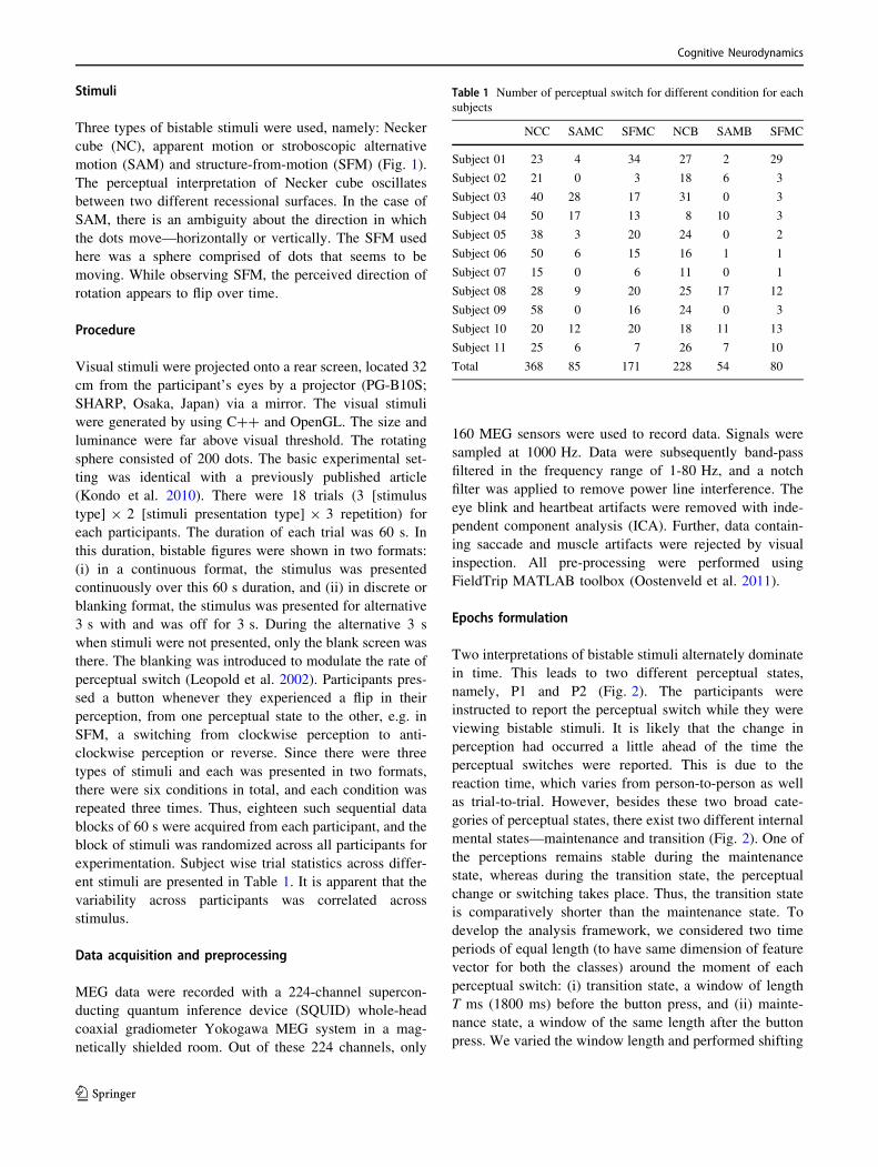
experimentation. Subject wise trial statistics across differ-

ent stimuli are presented in Table 1. It is apparent that the

variability across participants was correlated across

stimulus.

Data acquisition and preprocessing

MEG data were recorded with a 224-channel supercon-

ducting quantum inference device (SQUID) whole-head

coaxial gradiometer Yokogawa MEG system in a mag-

netically shielded room. Out of these 224 channels, only

160 MEG sensors were used to record data. Signals were

sampled at 1000 Hz. Data were subsequently band-pass

filtered in the frequency range of 1-80 Hz, and a notch

filter was applied to remove power line interference. The

eye blink and heartbeat artifacts were removed with inde-

pendent component analysis (ICA). Further, data contain-

ing saccade and muscle artifacts were rejected by visual

inspection. All pre-processing were performed using

FieldTrip MATLAB toolbox (Oostenveld et al. 2011).

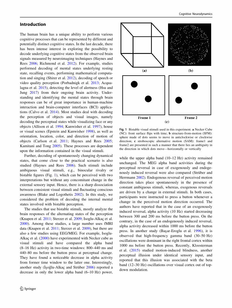
Epochs formulation

Two interpretations of bistable stimuli alternately dominate

in time. This leads to two different perceptual states,

namely, P1 and P2 (Fig. 2). The participants were

instructed to report the perceptual switch while they were

viewing bistable stimuli. It is likely that the change in

perception had occurred a little ahead of the time the

perceptual switches were reported. This is due to the

reaction time, which varies from person-to-person as well

as trial-to-trial. However, besides these two broad cate-

gories of perceptual states, there exist two different internal

mental states—maintenance and transition (Fig. 2). One of

the perceptions remains stable during the maintenance

state, whereas during the transition state, the perceptual

change or switching takes place. Thus, the transition state

is comparatively shorter than the maintenance state. To

develop the analysis framework, we considered two time

periods of equal length (to have same dimension of feature

vector for both the classes) around the moment of each

perceptual switch: (i) transition state, a window of length

T ms (1800 ms) before the button press, and (ii) mainte-

nance state, a window of the same length after the button

press. We varied the window length and performed shifting

Table 1 Number of perceptual switch for different condition for each

subjects

NCC SAMC SFMC NCB SAMB SFMC

Subject 01 23 4 34 27 2 29

Subject 02 21 0 3 18 6 3

Subject 03 40 28 17 31 0 3

Subject 04 50 17 13 8 10 3

Subject 05 38 3 20 24 0 2

Subject 06 50 6 15 16 1 1

Subject 07 15 0 6 11 0 1

Subject 08 28 9 20 25 17 12

Subject 09 58 0 16 24 0 3

Subject 10 20 12 20 18 11 13

Subject 11 25 6 7 26 7 10

Total 368 85 171 228 54 80

Cognitive Neurodynamics

123

the window for further analysis. We also treated this as a

classification problem where transition and maintenance

states were treated as two different classes. The considered

transition and maintenance states are shown in Fig. 2. The

trials with overlapped maintenance state with the next

transition or overlapped transition state with previous

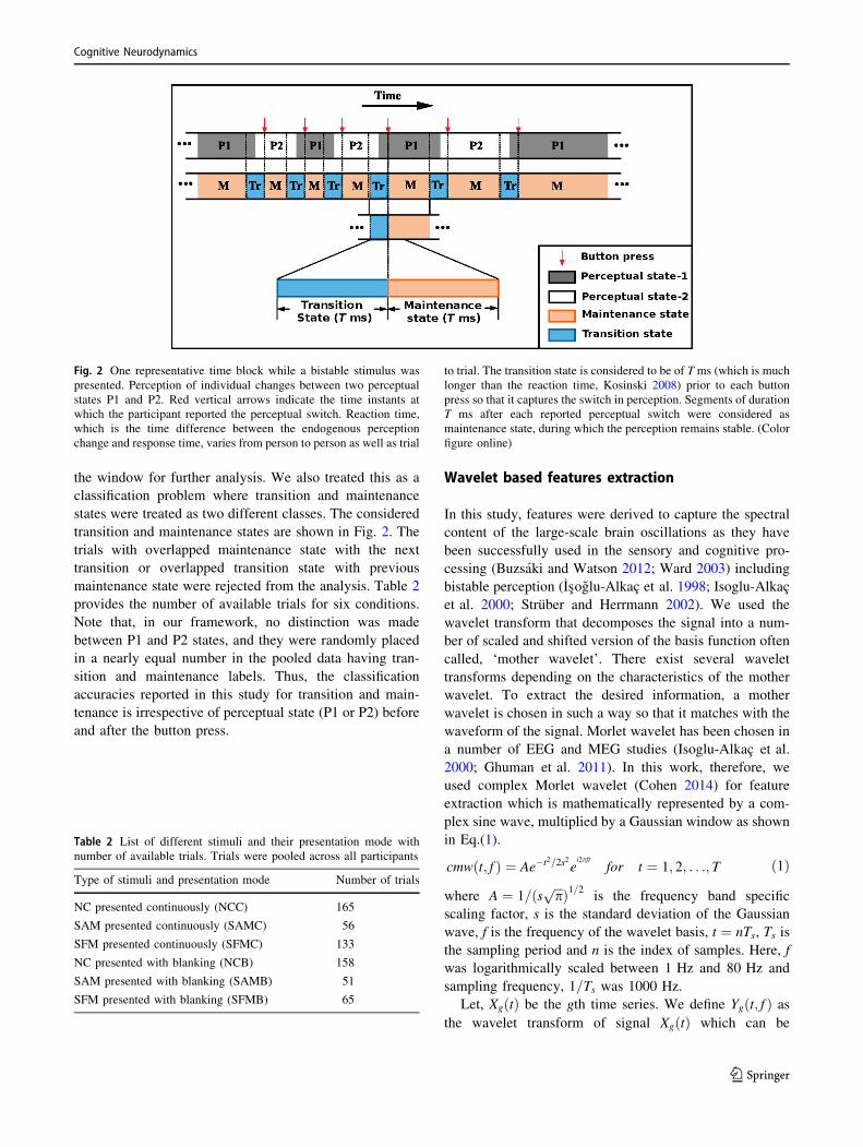
maintenance state were rejected from the analysis. Table 2

provides the number of available trials for six conditions.

Note that, in our framework, no distinction was made

between P1 and P2 states, and they were randomly placed

in a nearly equal number in the pooled data having tran-

sition and maintenance labels. Thus, the classification

accuracies reported in this study for transition and main-

tenance is irrespective of perceptual state (P1 or P2) before

and after the button press.

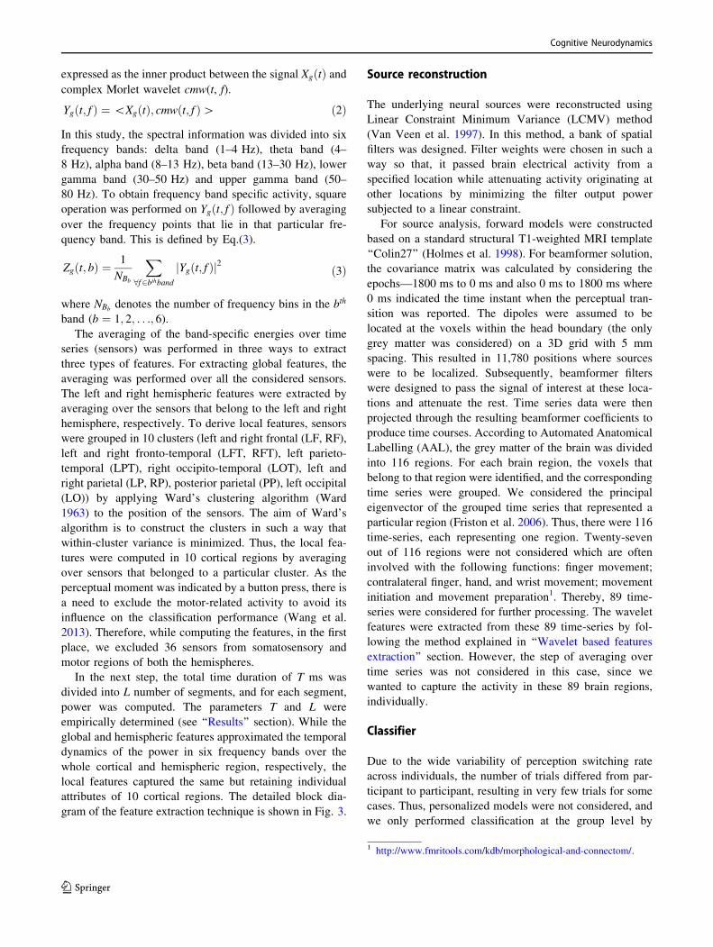
Wavelet based features extraction

In this study, features were derived to capture the spectral

content of the large-scale brain oscillations as they have

been successfully used in the sensory and cognitive pro-

cessing (Buzsaki and Watson 2012; Ward 2003) including

bistable perception (Isoglu-Alkac et al. 1998; Isoglu-Alkac

et al. 2000; Struber and Herrmann 2002). We used the

wavelet transform that decomposes the signal into a num-

ber of scaled and shifted version of the basis function often

called, ‘mother wavelet’. There exist several wavelet

transforms depending on the characteristics of the mother

wavelet. To extract the desired information, a mother

wavelet is chosen in such a way so that it matches with the

waveform of the signal. Morlet wavelet has been chosen in

a number of EEG and MEG studies (Isoglu-Alkac et al.

2000; Ghuman et al. 2011). In this work, therefore, we

used complex Morlet wavelet (Cohen 2014) for feature

extraction which is mathematically represented by a com-

plex sine wave, multiplied by a Gaussian window as shown

in Eq.(1).

cmwðt; f Þ ¼ Ae�t2=2s2ei2pft

for t ¼ 1; 2; . . .; T ð1Þ

where A ¼ 1=ðsffiffiffi

pp

Þ1=2 is the frequency band specific

scaling factor, s is the standard deviation of the Gaussian

wave, f is the frequency of the wavelet basis, t ¼ nTs, Ts is

the sampling period and n is the index of samples. Here, f

was logarithmically scaled between 1 Hz and 80 Hz and

sampling frequency, 1=Ts was 1000 Hz.

Let, XgðtÞ be the gth time series. We define Ygðt; f Þ as

the wavelet transform of signal XgðtÞ which can be

Fig. 2 One representative time block while a bistable stimulus was

presented. Perception of individual changes between two perceptual

states P1 and P2. Red vertical arrows indicate the time instants at

which the participant reported the perceptual switch. Reaction time,

which is the time difference between the endogenous perception

change and response time, varies from person to person as well as trial

to trial. The transition state is considered to be of Tms (which is much

longer than the reaction time, Kosinski 2008) prior to each button

press so that it captures the switch in perception. Segments of duration

T ms after each reported perceptual switch were considered as

maintenance state, during which the perception remains stable. (Color

figure online)

Table 2 List of different stimuli and their presentation mode with

number of available trials. Trials were pooled across all participants

Type of stimuli and presentation mode Number of trials

NC presented continuously (NCC) 165

SAM presented continuously (SAMC) 56

SFM presented continuously (SFMC) 133

NC presented with blanking (NCB) 158

SAM presented with blanking (SAMB) 51

SFM presented with blanking (SFMB) 65

Cognitive Neurodynamics

123

expressed as the inner product between the signal XgðtÞ andcomplex Morlet wavelet cmw(t, f).

Ygðt; f Þ ¼ \XgðtÞ; cmwðt; f Þ[ ð2Þ

In this study, the spectral information was divided into six

frequency bands: delta band (1–4 Hz), theta band (4–

8 Hz), alpha band (8–13 Hz), beta band (13–30 Hz), lower

gamma band (30–50 Hz) and upper gamma band (50–

80 Hz). To obtain frequency band specific activity, square

operation was performed on Ygðt; f Þ followed by averaging

over the frequency points that lie in that particular fre-

quency band. This is defined by Eq.(3).

Zgðt; bÞ ¼1

NBb

X

8f2bthbandjYgðt; f Þj2 ð3Þ

where NBbdenotes the number of frequency bins in the bth

band (b ¼ 1; 2; . . .; 6).

The averaging of the band-specific energies over time

series (sensors) was performed in three ways to extract

three types of features. For extracting global features, the

averaging was performed over all the considered sensors.

The left and right hemispheric features were extracted by

averaging over the sensors that belong to the left and right

hemisphere, respectively. To derive local features, sensors

were grouped in 10 clusters (left and right frontal (LF, RF),

left and right fronto-temporal (LFT, RFT), left parieto-

temporal (LPT), right occipito-temporal (LOT), left and

right parietal (LP, RP), posterior parietal (PP), left occipital

(LO)) by applying Ward’s clustering algorithm (Ward

1963) to the position of the sensors. The aim of Ward’s

algorithm is to construct the clusters in such a way that

within-cluster variance is minimized. Thus, the local fea-

tures were computed in 10 cortical regions by averaging

over sensors that belonged to a particular cluster. As the

perceptual moment was indicated by a button press, there is

a need to exclude the motor-related activity to avoid its

influence on the classification performance (Wang et al.

2013). Therefore, while computing the features, in the first

place, we excluded 36 sensors from somatosensory and

motor regions of both the hemispheres.

In the next step, the total time duration of T ms was

divided into L number of segments, and for each segment,

power was computed. The parameters T and L were

empirically determined (see ‘‘Results’’ section). While the

global and hemispheric features approximated the temporal

dynamics of the power in six frequency bands over the

whole cortical and hemispheric region, respectively, the

local features captured the same but retaining individual

attributes of 10 cortical regions. The detailed block dia-

gram of the feature extraction technique is shown in Fig. 3.

Source reconstruction

The underlying neural sources were reconstructed using

Linear Constraint Minimum Variance (LCMV) method

(Van Veen et al. 1997). In this method, a bank of spatial

filters was designed. Filter weights were chosen in such a

way so that, it passed brain electrical activity from a

specified location while attenuating activity originating at

other locations by minimizing the filter output power

subjected to a linear constraint.

For source analysis, forward models were constructed

based on a standard structural T1-weighted MRI template

‘‘Colin27’’ (Holmes et al. 1998). For beamformer solution,

the covariance matrix was calculated by considering the

epochs—1800 ms to 0 ms and also 0 ms to 1800 ms where

0 ms indicated the time instant when the perceptual tran-

sition was reported. The dipoles were assumed to be

located at the voxels within the head boundary (the only

grey matter was considered) on a 3D grid with 5 mm

spacing. This resulted in 11,780 positions where sources

were to be localized. Subsequently, beamformer filters

were designed to pass the signal of interest at these loca-

tions and attenuate the rest. Time series data were then

projected through the resulting beamformer coefficients to

produce time courses. According to Automated Anatomical

Labelling (AAL), the grey matter of the brain was divided

into 116 regions. For each brain region, the voxels that

belong to that region were identified, and the corresponding

time series were grouped. We considered the principal

eigenvector of the grouped time series that represented a

particular region (Friston et al. 2006). Thus, there were 116

time-series, each representing one region. Twenty-seven

out of 116 regions were not considered which are often

involved with the following functions: finger movement;

contralateral finger, hand, and wrist movement; movement

initiation and movement preparation1. Thereby, 89 time-

series were considered for further processing. The wavelet

features were extracted from these 89 time-series by fol-

lowing the method explained in ‘‘Wavelet based features

extraction’’ section. However, the step of averaging over

time series was not considered in this case, since we

wanted to capture the activity in these 89 brain regions,

individually.

Classifier

Due to the wide variability of perception switching rate

across individuals, the number of trials differed from par-

ticipant to participant, resulting in very few trials for some

cases. Thus, personalized models were not considered, and

we only performed classification at the group level by

1 http://www.fmritools.com/kdb/morphological-and-connectom/.

Cognitive Neurodynamics

123

pooling trials across all participants (Table 2). We used

SVM (Vapnik 2013) classifier with Radial Basis Function

(RBF) as the kernel function, and also, ANN classifier. The

application of SVM and ANN classifier has been found in

various studies related to the classification of to neuro-

signal (Alimardani et al. 2013; Subasi 2005). For ANN

classifier, the number of nodes at the hidden layer was fixed

at 10. Scale-conjugate gradient backpropagation algorithm

was used to train the model. Mean square error was set to

10-5, and the hyperbolic tangent sigmoid transfer function

was used as the activation function.

The performance of the classifier was evaluated using

10-fold cross-validation. It is considered more reliable

compared to leave-one-out cross-validation (Varoquaux

et al. 2017). Of note, the data to train the classifier and the

data to test its performance were mutually exclusive. The

performance of the classifier was measured by accuracy,

sensitivity, and specificity; where sensitivity and specificity

quantify how accurately the model was able to detect the

transition, and maintenance states, respectively. All

analysis was performed using customized scripts using

MATLAB 2013a.

Results

We aim to classify the two internal mental states that

involve different complex cognitive processing. In a

number of earlier studies, the oscillatory activities in the

alpha, beta and gamma band were found to play important

role in bistable perception as well as complex cognitive

processing (Piantoni et al. 2017; Lange et al. 2014; Pian-

toni et al. 2010; Okazaki et al. 2008; Kloosterman et al.

2015; Keil et al. 1999; Basar-Eroglu et al. 1996). So, we

validated this on our data by using Bonferroni corrected t-

test between trials from transition and maintenance states

of whole epoch for all six frequency bands considered in

this study. The difference between the transition/mainte-

nance states was found to be significant

(p\0:05=6 ¼ 0:0083) for the following bands: alpha

Fig. 3 Different steps involved in the feature extraction process.

Complex Morlet wavelet transform was applied on the T ms length

time series data. To obtain band-specific energy, the wavelet

coefficients of wavelet transform were squared and averaged over

the frequency points that belong to a specific frequency band [Delta

(1–4 Hz), Theta (4–8 Hz), Alpha (8–13 Hz), Beta (13–30), lower

Gamma (30–50 Hz) and upper Gamma (50–80 Hz)]. Three types of

the feature were extracted—global feature, hemispheric (left and

right) feature and local feature. To extract global, hemispheric and

local features, frequency band energies were averaged over all the

sensors, sensors that belonged to particular hemisphere and sensors

that belong to a particular region, respectively. In all these three cases,

the sensors from the motor cortex were excluded. The temporal

dynamics of these features were approximated by diving T ms into

L segments and averaged over the time points of each segment

separately

Cognitive Neurodynamics

123

[tð627Þ ¼ � 4:9256, p\0:0083], beta

[tð627Þ ¼ � 10:3515, p\0:0083], lower gamma

[tð627Þ ¼ � 12:3498, p\0:0083], and upper gamma

[tð627Þ ¼ � 6:9995, p\0:0083]. Thus, we used features

from these fours bands to predict the mental states on a

single-trial basis.

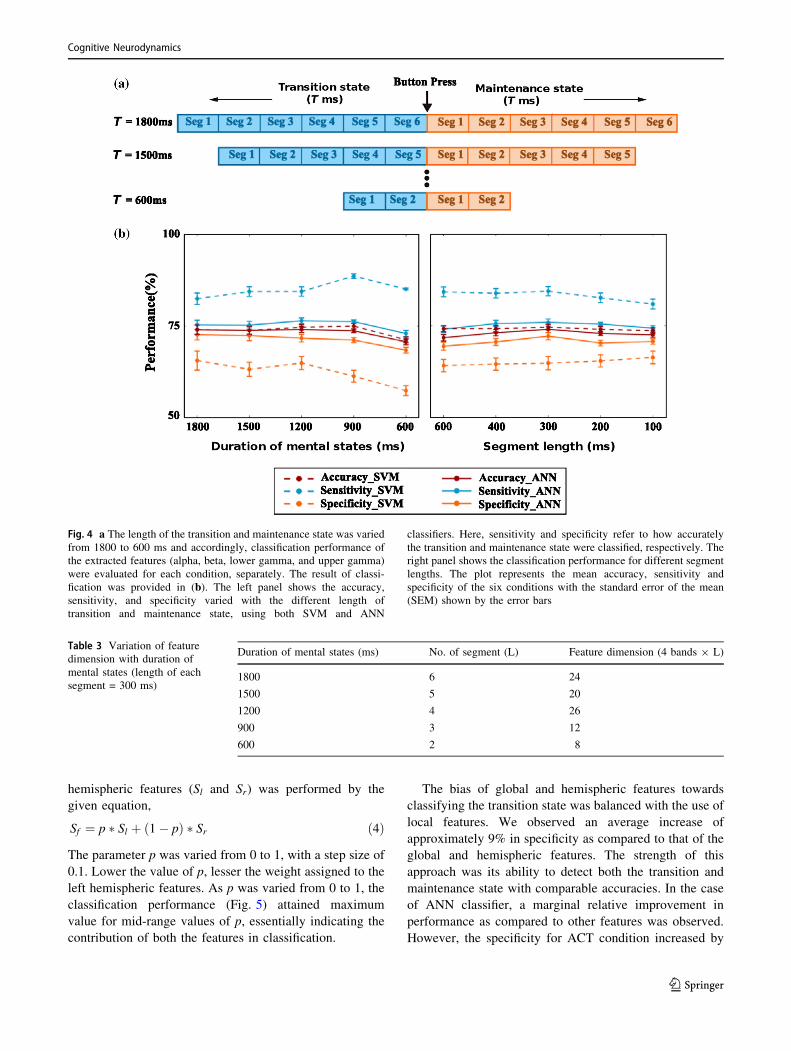
Effective duration of transition state

The participants indicated perceptual reversal by pressing a

button. However, the reaction time might vary across

participants as well as from trial-to-trial. Additionally,

some transition occurs instantaneously whereas ‘‘other

transitions comprise the dynamic mixture of both the per-

cepts for variable periods before one percept dominates

completely’’ (Knapen et al. 2011), thus leading to a vari-

able duration of the transition state. To determine the

effective time-duration that best represents the transition

state, we considered the different extents of transition state

varying from 600 to 1800 ms in steps of 300 ms. To retain

the same feature dimension for both the classes, the length

of the maintenance state was kept the same as the length of

the transition state. Figure 4a shows the different transition

and maintenance states considered for the analysis. For

each case, the global feature was extracted from the alpha,

beta, lower gamma, and upper gamma frequency band

using segment length l ¼ T=L of 300 ms and then used in

classification. Table 3 shows the feature dimension for

different length of the transition state. The classification

performance, i.e. accuracy, sensitivity, and specificity

concerning the length of the transition state, are shown on

the left panel of Fig. 4b.

Since accuracy, sensitivity, and specificity for the length

of 1200 ms were comparatively good and adequate for all

the conditions and both classifiers, it was considered as the

effective length of the transition state and used for further

analysis. Next, we analyzed the performance variation with

respect to the segment length, which was kept 300 ms

throughout the previous analysis. Here, we varied the

segment length from 100 to 600 ms (in steps of 100 ms),

and the extracted features were used for classification (right

panel of Fig. 4b). The classification performance remained

relatively stable across various segment lengths. Since the

segment length of 300 ms yielded the best accuracy, it was

considered for further analysis.

For classification of mental states, three types of features

were considered: (1) global features, (2) hemispheric (left

and right hemispheric) features, and (3) local brain region-

specific features. Along with the six conditions listed in

Table 2, we also pooled the trials irrespective of types of

condition, and their presentation mode is referred as ‘ACT’

(all conditions together) in this paper.

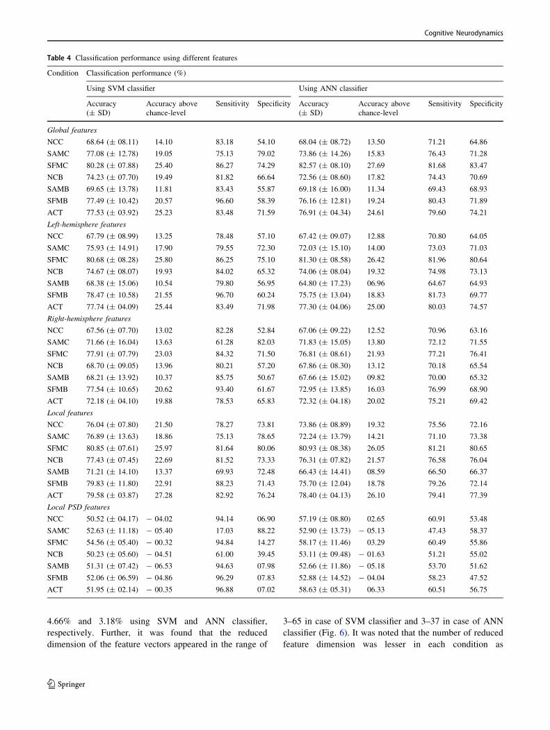
Single trial classification

We computed global, hemispheric, and local features in the

alpha, beta, lower gamma, and upper gamma frequency

band for transition and maintenance states of a duration of

1200 ms. The feature dimension for global, hemispheric,

and local features were 16, 16, and 160, respectively. A

10-fold cross-validation was performed to evaluate the

performance. In the case of local features, we used PCA to

reduce the feature dimension. The PCA was applied to the

training data of 9 folds, and the new dimension was

determined from the principal components that capture

Cv% (cumulative variance) of the total variance. The

cumulative variance was varied from 95 to 99.9%, and the

classification performances of training data were computed

using 10-fold inner cross-validation. The Cv and the new

dimension was determined from the value of the cumula-

tive variance at which the best performance was obtained.

Using this new dimension, the classification model was

built from training data (9 folds), and the test performance

was determined from the remaining one fold. This proce-

dure was repeated in each run of 10 fold cross-validation,

and average test performance was computed. Table 4

shows the classification performance of different features

using SVM and ANN classifiers for each of the six con-

ditions and also for ACT. We observed that the classifi-

cation performance of all the features was substantially

higher than the empirical chance level. Of note, while the

theoretical chance level accuracy is 50% as there are only

two classes, the chance level accuracy is liable to increase

in the presence of a small number of data samples and is

referred to as the empirical chance level. It was determined

using the method in Combrisson and Jerbi (2015), which

assumes that the classification errors obey a cumulative

binomial distribution.

Among the wavelet features, the local features per-

formed better than global and hemispheric features; the

former yielded a better balance between sensitivity and

specificity for both SVM and ANN classifiers. The sensi-

tivity for global and hemisphere-specific features for all

condition was higher than the indicating that the transition

state was classified more accurately than the maintenance

state at the global and hemispheric brain level. The left

hemispheric features performed relatively better as com-

pared to that of right hemispheric features indicating a

greater contribution of left hemispheric features towards

distinguishing the two classes. Alternatively, these two

types of features may also capture complementary infor-

mation. Thus, we performed an analysis by predicting the

states by combining the scores obtained from both the

features. The integration of the scores from left and right

Cognitive Neurodynamics

123

hemispheric features (Sl and Sr) was performed by the

given equation,

Sf ¼ p � Sl þ ð1� pÞ � Sr ð4Þ

The parameter p was varied from 0 to 1, with a step size of

0.1. Lower the value of p, lesser the weight assigned to the

left hemispheric features. As p was varied from 0 to 1, the

classification performance (Fig. 5) attained maximum

value for mid-range values of p, essentially indicating the

contribution of both the features in classification.

The bias of global and hemispheric features towards

classifying the transition state was balanced with the use of

local features. We observed an average increase of

approximately 9% in specificity as compared to that of the

global and hemispheric features. The strength of this

approach was its ability to detect both the transition and

maintenance state with comparable accuracies. In the case

of ANN classifier, a marginal relative improvement in

performance as compared to other features was observed.

However, the specificity for ACT condition increased by

Fig. 4 a The length of the transition and maintenance state was varied

from 1800 to 600 ms and accordingly, classification performance of

the extracted features (alpha, beta, lower gamma, and upper gamma)

were evaluated for each condition, separately. The result of classi-

fication was provided in (b). The left panel shows the accuracy,

sensitivity, and specificity varied with the different length of

transition and maintenance state, using both SVM and ANN

classifiers. Here, sensitivity and specificity refer to how accurately

the transition and maintenance state were classified, respectively. The

right panel shows the classification performance for different segment

lengths. The plot represents the mean accuracy, sensitivity and

specificity of the six conditions with the standard error of the mean

(SEM) shown by the error bars

Table 3 Variation of feature

dimension with duration of

mental states (length of each

segment = 300 ms)

Duration of mental states (ms) No. of segment (L) Feature dimension (4 bands 9 L)

1800 6 24

1500 5 20

1200 4 26

900 3 12

600 2 8

Cognitive Neurodynamics

123

4.66% and 3.18% using SVM and ANN classifier,

respectively. Further, it was found that the reduced

dimension of the feature vectors appeared in the range of

3–65 in case of SVM classifier and 3–37 in case of ANN

classifier (Fig. 6). It was noted that the number of reduced

feature dimension was lesser in each condition as

Table 4 Classification performance using different features

Condition Classification performance (%)

Using SVM classifier Using ANN classifier

Accuracy

(± SD)

Accuracy above

chance-level

Sensitivity Specificity Accuracy

(± SD)

Accuracy above

chance-level

Sensitivity Specificity

Global features

NCC 68.64 (± 08.11) 14.10 83.18 54.10 68.04 (± 08.72) 13.50 71.21 64.86

SAMC 77.08 (± 12.78) 19.05 75.13 79.02 73.86 (± 14.26) 15.83 76.43 71.28

SFMC 80.28 (± 07.88) 25.40 86.27 74.29 82.57 (± 08.10) 27.69 81.68 83.47

NCB 74.23 (± 07.70) 19.49 81.82 66.64 72.56 (± 08.60) 17.82 74.43 70.69

SAMB 69.65 (± 13.78) 11.81 83.43 55.87 69.18 (± 16.00) 11.34 69.43 68.93

SFMB 77.49 (± 10.42) 20.57 96.60 58.39 76.16 (± 12.81) 19.24 80.43 71.89

ACT 77.53 (± 03.92) 25.23 83.48 71.59 76.91 (± 04.34) 24.61 79.60 74.21

Left-hemisphere features

NCC 67.79 (± 08.99) 13.25 78.48 57.10 67.42 (± 09.07) 12.88 70.80 64.05

SAMC 75.93 (± 14.91) 17.90 79.55 72.30 72.03 (± 15.10) 14.00 73.03 71.03

SFMC 80.68 (± 08.28) 25.80 86.25 75.10 81.30 (± 08.58) 26.42 81.96 80.64

NCB 74.67 (± 08.07) 19.93 84.02 65.32 74.06 (± 08.04) 19.32 74.98 73.13

SAMB 68.38 (± 15.06) 10.54 79.80 56.95 64.80 (± 17.23) 06.96 64.67 64.93

SFMB 78.47 (± 10.58) 21.55 96.70 60.24 75.75 (± 13.04) 18.83 81.73 69.77

ACT 77.74 (± 04.09) 25.44 83.49 71.98 77.30 (± 04.06) 25.00 80.03 74.57

Right-hemisphere features

NCC 67.56 (± 07.70) 13.02 82.28 52.84 67.06 (± 09.22) 12.52 70.96 63.16

SAMC 71.66 (± 16.04) 13.63 61.28 82.03 71.83 (± 15.05) 13.80 72.12 71.55

SFMC 77.91 (± 07.79) 23.03 84.32 71.50 76.81 (± 08.61) 21.93 77.21 76.41

NCB 68.70 (± 09.05) 13.96 80.21 57.20 67.86 (± 08.30) 13.12 70.18 65.54

SAMB 68.21 (± 13.92) 10.37 85.75 50.67 67.66 (± 15.02) 09.82 70.00 65.32

SFMB 77.54 (± 10.65) 20.62 93.40 61.67 72.95 (± 13.85) 16.03 76.99 68.90

ACT 72.18 (± 04.10) 19.88 78.53 65.83 72.32 (± 04.18) 20.02 75.21 69.42

Local features

NCC 76.04 (± 07.80) 21.50 78.27 73.81 73.86 (± 08.89) 19.32 75.56 72.16

SAMC 76.89 (± 13.63) 18.86 75.13 78.65 72.24 (± 13.79) 14.21 71.10 73.38

SFMC 80.85 (± 07.61) 25.97 81.64 80.06 80.93 (± 08.38) 26.05 81.21 80.65

NCB 77.43 (± 07.45) 22.69 81.52 73.33 76.31 (± 07.82) 21.57 76.58 76.04

SAMB 71.21 (± 14.10) 13.37 69.93 72.48 66.43 (± 14.41) 08.59 66.50 66.37

SFMB 79.83 (± 11.80) 22.91 88.23 71.43 75.70 (± 12.04) 18.78 79.26 72.14

ACT 79.58 (± 03.87) 27.28 82.92 76.24 78.40 (± 04.13) 26.10 79.41 77.39

Local PSD features

NCC 50.52 (± 04.17) - 04.02 94.14 06.90 57.19 (± 08.80) 02.65 60.91 53.48

SAMC 52.63 (± 11.18) - 05.40 17.03 88.22 52.90 (± 13.73) - 05.13 47.43 58.37

SFMC 54.56 (± 05.40) - 00.32 94.84 14.27 58.17 (± 11.46) 03.29 60.49 55.86

NCB 50.23 (± 05.60) - 04.51 61.00 39.45 53.11 (± 09.48) - 01.63 51.21 55.02

SAMB 51.31 (± 07.42) - 06.53 94.63 07.98 52.66 (± 11.86) - 05.18 53.70 51.62

SFMB 52.06 (± 06.59) - 04.86 96.29 07.83 52.88 (± 14.52) - 04.04 58.23 47.52

ACT 51.95 (± 02.14) - 00.35 96.88 07.02 58.63 (± 05.31) 06.33 60.51 56.75

Cognitive Neurodynamics

123

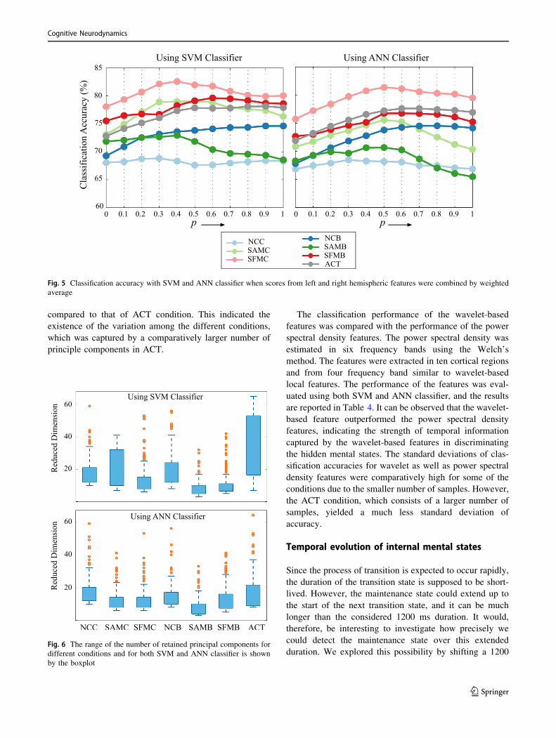
compared to that of ACT condition. This indicated the

existence of the variation among the different conditions,

which was captured by a comparatively larger number of

principle components in ACT.

The classification performance of the wavelet-based

features was compared with the performance of the power

spectral density features. The power spectral density was

estimated in six frequency bands using the Welch’s

method. The features were extracted in ten cortical regions

and from four frequency band similar to wavelet-based

local features. The performance of the features was eval-

uated using both SVM and ANN classifier, and the results

are reported in Table 4. It can be observed that the wavelet-

based feature outperformed the power spectral density

features, indicating the strength of temporal information

captured by the wavelet-based features in discriminating

the hidden mental states. The standard deviations of clas-

sification accuracies for wavelet as well as power spectral

density features were comparatively high for some of the

conditions due to the smaller number of samples. However,

the ACT condition, which consists of a larger number of

samples, yielded a much less standard deviation of

accuracy.

Temporal evolution of internal mental states

Since the process of transition is expected to occur rapidly,

the duration of the transition state is supposed to be short-

lived. However, the maintenance state could extend up to

the start of the next transition state, and it can be much

longer than the considered 1200 ms duration. It would,

therefore, be interesting to investigate how precisely we

could detect the maintenance state over this extended

duration. We explored this possibility by shifting a 1200

Fig. 5 Classification accuracy with SVM and ANN classifier when scores from left and right hemispheric features were combined by weighted

average

Fig. 6 The range of the number of retained principal components for

different conditions and for both SVM and ANN classifier is shown

by the boxplot

Cognitive Neurodynamics

123

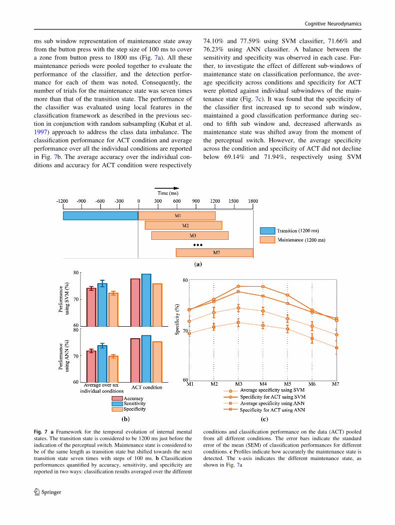
ms sub window representation of maintenance state away

from the button press with the step size of 100 ms to cover

a zone from button press to 1800 ms (Fig. 7a). All these

maintenance periods were pooled together to evaluate the

performance of the classifier, and the detection perfor-

mance for each of them was noted. Consequently, the

number of trials for the maintenance state was seven times

more than that of the transition state. The performance of

the classifier was evaluated using local features in the

classification framework as described in the previous sec-

tion in conjunction with random subsampling (Kubat et al.

1997) approach to address the class data imbalance. The

classification performance for ACT condition and average

performance over all the individual conditions are reported

in Fig. 7b. The average accuracy over the individual con-

ditions and accuracy for ACT condition were respectively

74.10% and 77.59% using SVM classifier, 71.66% and

76.23% using ANN classifier. A balance between the

sensitivity and specificity was observed in each case. Fur-

ther, to investigate the effect of different sub-windows of

maintenance state on classification performance, the aver-

age specificity across conditions and specificity for ACT

were plotted against individual subwindows of the main-

tenance state (Fig. 7c). It was found that the specificity of

the classifier first increased up to second sub window,

maintained a good classification performance during sec-

ond to fifth sub window and, decreased afterwards as

maintenance state was shifted away from the moment of

the perceptual switch. However, the average specificity

across the condition and specificity of ACT did not decline

below 69.14% and 71.94%, respectively using SVM

Fig. 7 a Framework for the temporal evolution of internal mental

states. The transition state is considered to be 1200 ms just before the

indication of the perceptual switch. Maintenance state is considered to

be of the same length as transition state but shifted towards the next

transition state seven times with steps of 100 ms. b Classification

performances quantified by accuracy, sensitivity, and specificity are

reported in two ways: classification results averaged over the different

conditions and classification performance on the data (ACT) pooled

from all different conditions. The error bars indicate the standard

error of the mean (SEM) of classification performances for different

conditions. c Profiles indicate how accurately the maintenance state is

detected. The x-axis indicates the different maintenance state, as

shown in Fig. 7a

Cognitive Neurodynamics

123

classifier and were found to be 66.57% and 72.37%,

respectively using ANN classifier.

Role of underlying brain sources in classificationof mental states

In this section, we investigate the brain regions involved in

the transition and maintenance state. For that purpose, we

estimated the time series data in source domain recon-

structed from MEG data recorded at sensor level and

extracted the features in source domain by following the

same feature extraction method as discussed in ‘‘Wavelet

based features extraction’’ section and ‘‘Source recon-

struction’’ section, respectively. This analysis in source

domain would identify the neural sources in the brain

rather than its projected effect on the scalp level. We have

employed the framework used in the previous section

(‘‘Temporal evolution of internal mental states’’ section)

that took into consideration the wider maintenance state

duration. We considered local features extracted from

reconstructed sources in six frequency bands and 89 brain

regions for classification using SVM and ANN classifier.

Here, we used F-ratio based feature selection technique

instead of PCA, as in the latter, data was projected on the

direction of principal components that leads to loss of

information as regards to one specific source of the feature.

F-ratio is computed as the ratio of between-class variance

to the total within-class variance. A larger F-ratio indicates

a greater separability between the classes, thus essentially

implying more effective feature to discriminate the classes.

The features with largest F-ratio were given highest pri-

ority. Thus, besides the classification performance, this

analysis also found discriminative and dominant features

by analyzing the features which were selected at the

training stage. This, in turn, led to the identification of the

underlying neural sources which responded differently

during two mental states within a particular frequency

band.

In this method, we were able to classify the mental states

with an average (averaged over six conditions) accuracy of

73.55% and 71.19% using SVM and ANN classifier,

respectively; 74.98% and 73.05% accuracy using SVM and

ANN classifier, respectively when ACT condition was

considered. We analyzed the source features that were

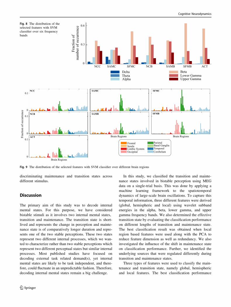
selected at the training stage in each fold. Figure 8 shows

the distribution of selected features over different fre-

quency bands. The dominance of features from alpha, beta,

lower gamma, and upper gamma frequency band was

noticed, consolidating our earlier sensor space based find-

ings. The distribution of the selected features over brain

regions (Fig. 9) showed that the features were selected in

the majority from parietal, occipital and cerebellum area.

Thus, the sources of these areas were modulated differently

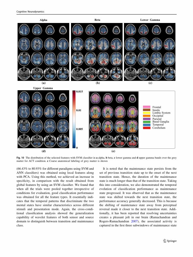
during the state of transition and maintenance. Figure 10

shows the distribution of the selected features over

anatomical brain regions for each of the highly contributing

frequency bands for ACT conditions. The weights indicate

the fraction of the number of selected features from that

region. The weights of the excluded regions were set to

zero for visualization. The rightmost panel shows the

coarse labelling of grey matter according to AAL for ref-

erence. The features from parietal regions were found to be

consistently selected in the majority from alpha, beta,

lower and upper gamma frequency band. Besides this, the

occipital and cerebellum regions were found to be modu-

lated distinctly for two considered mental states in alpha,

beta and lower gamma frequency bands. The analysis of

selected features using SVM and ANN classifier showed a

similar result. In Figs. 8, 9 and 10 we have presented the

result of the analysis using SVM classifier which are

similar for ANN classifier.

Cross-conditional classification

In the above sections, we evaluated the performance of

different features under six conditions (three types of

stimuli and two ways of presentation). For evaluating the

performance for a condition, the data of that condition was

divided into training and testing sets; training data was

used to build the model and testing data to evaluate the

model performance. Again, in the case of ACT, where the

data from all the condition were pooled together, the data

were treated irrespective of the corresponding condition

and followed the same procedure to evaluate the perfor-

mance. It is interesting to investigate the generalisation of

classifier across different stimulus types. Therefore, in this

section, we have considered the cross-conditional classifi-

cation by building the model using the data of one stimulus

and testing on the data of others. Instead of considering all

the conditions separately, only three stimuli factors

(Necker Cube, Stroboscopic Alternative Motion and

Structure From Motion) were taken into account irrespec-

tive of the stimuli presentation style. This study reveals the

cross-conditional generalization power of the features

(Peelen et al. 2010) we used for classification purpose.

Table 5 represents the cross-classification performances of

sensor-based global, hemispheric and local features using

SVM and ANN classifiers. This analysis was extended to

senor and source based local features in the framework

explained in ‘‘Temporal evolution of internal mental

states’’ section and the result is presented in Table 6. It was

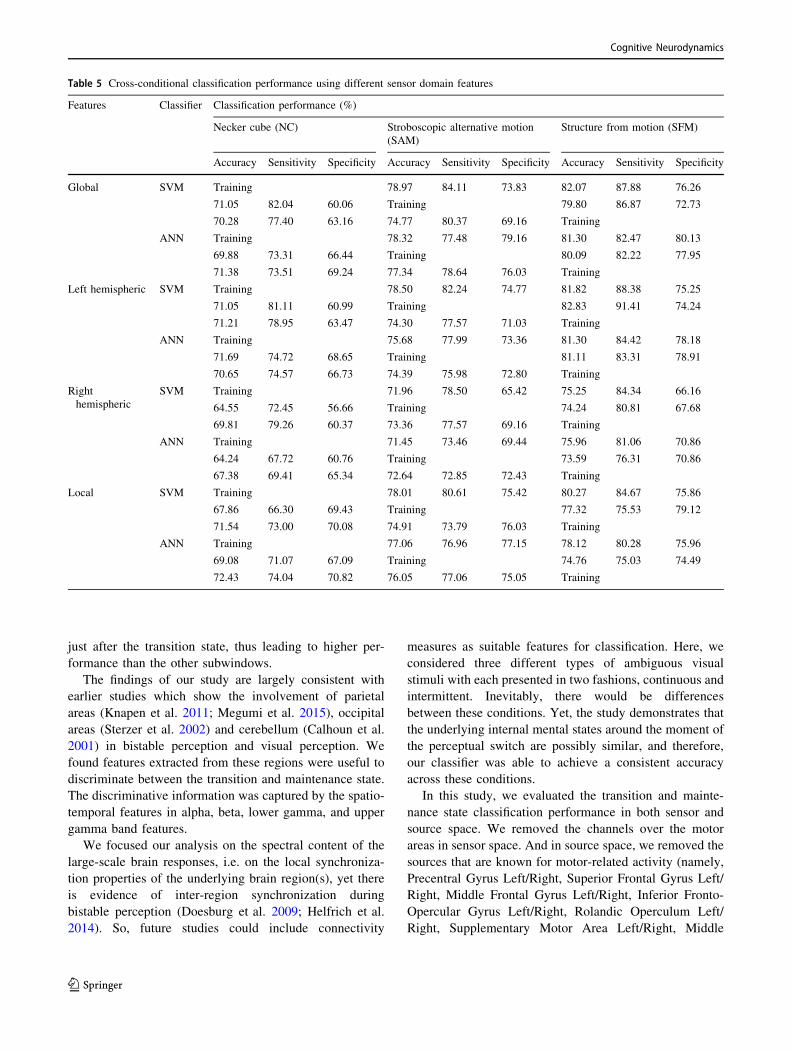
found that cross-conditional classification performances

were comparable with the classification result obtained in

the previous three sections. We may conclude that brain

responses captured by wavelet features are generalized in

Cognitive Neurodynamics

123

discriminating maintenance and transition states across

different stimulus.

Discussion

The primary aim of this study was to decode internal

mental states. For this purpose, we have considered

bistable stimuli as it involves two internal mental states,

transition and maintenance. The transition state is short-

lived and represents the change in perception and mainte-

nance state is of comparatively longer duration and repre-

sents one of the two stable perceptions. These two states

represent two different internal processes, which we wan-

ted to characterize rather than two stable perceptions which

represent two different perceptual states but similar internal

processes. Most published studies have focused on

decoding external task related demand(s), yet internal

mental states are likely to be task independent, and there-

fore, could fluctuate in an unpredictable fashion. Therefore,

decoding internal mental states remain a big challenge.

In this study, we classified the transition and mainte-

nance states involved in bistable perception using MEG

data on a single-trial basis. This was done by applying a

machine learning framework to the spatiotemporal

dynamics of large-scale brain oscillations. To capture this

temporal information, three different features were derived

(global, hemispheric and local) using wavelet subband

energies in the alpha, beta, lower gamma, and upper

gamma frequency bands. We also determined the effective

transition state by evaluating the classification performance

on different lengths of transition and maintenance state.

The best classification result was obtained when local

region based features were used along with the PCA to

reduce feature dimension as well as redundancy. We also

investigated the influence of the shift in maintenance state

on classification performance. Further, we identified the

underlying sources that were regulated differently during

transition and maintenance states.

Three types of features were used to classify the main-

tenance and transition state, namely global, hemispheric

and local features. The best classification performance

Fig. 8 The distribution of the

selected features with SVM

classifier over six frequency

bands

Fig. 9 The distribution of the selected features with SVM classifier over different brain regions

Cognitive Neurodynamics

123

(66.43% to 80.93% for different paradigms using SVM and

ANN classifiers) was obtained using local features along

with PCA. Using this method, we achieved an increase in

specificity, in comparison with the result obtained from

global features by using an SVM classifier. We found that

when all the trials were pooled together irrespective of

conditions for evaluation, good classification performance

was obtained for all the feature types. It essentially indi-

cates that the temporal patterns that discriminate the two

mental states have similar characteristics across different

stimuli and presentation mode. Again, the cross-condi-

tional classification analysis showed the generalization

capability of wavelet features of both sensor and source

domain to distinguish between transition and maintenance

class.

It is noted that the maintenance state persists from the

set of previous transition state up to the onset of the next

transition state. Hence, the duration of the maintenance

state is much longer than that of the transition state. Taking

this into consideration, we also demonstrated the temporal

evolution of classification performance as maintenance

state progressed. It was observed that as the maintenance

state was shifted towards the next transition state, the

performance accuracy generally decreased. This is because

the shifting of maintenance state away from perceptual

reversal made it closer to the next transition state. Addi-

tionally, it has been reported that resolving uncertainties

creates a pleasant jolt in our brain (Ramachandran and

Rogers-Ramachandran 2007), the associated activity is

captured in the first three subwindows of maintenance state

(a)

(d) (e)

(b) (c)

Fig. 10 The distribution of the selected features with SVM classifier in a alpha, b beta, c lower gamma and d upper gamma bands over the grey

matter for ACT condition. e Coarse anatomical labeling of grey matter is shown

Cognitive Neurodynamics

123

just after the transition state, thus leading to higher per-

formance than the other subwindows.

The findings of our study are largely consistent with

earlier studies which show the involvement of parietal

areas (Knapen et al. 2011; Megumi et al. 2015), occipital

areas (Sterzer et al. 2002) and cerebellum (Calhoun et al.

2001) in bistable perception and visual perception. We

found features extracted from these regions were useful to

discriminate between the transition and maintenance state.

The discriminative information was captured by the spatio-

temporal features in alpha, beta, lower gamma, and upper

gamma band features.

We focused our analysis on the spectral content of the

large-scale brain responses, i.e. on the local synchroniza-

tion properties of the underlying brain region(s), yet there

is evidence of inter-region synchronization during

bistable perception (Doesburg et al. 2009; Helfrich et al.

2014). So, future studies could include connectivity

measures as suitable features for classification. Here, we

considered three different types of ambiguous visual

stimuli with each presented in two fashions, continuous and

intermittent. Inevitably, there would be differences

between these conditions. Yet, the study demonstrates that

the underlying internal mental states around the moment of

the perceptual switch are possibly similar, and therefore,

our classifier was able to achieve a consistent accuracy

across these conditions.

In this study, we evaluated the transition and mainte-

nance state classification performance in both sensor and

source space. We removed the channels over the motor

areas in sensor space. And in source space, we removed the

sources that are known for motor-related activity (namely,

Precentral Gyrus Left/Right, Superior Frontal Gyrus Left/

Right, Middle Frontal Gyrus Left/Right, Inferior Fronto-

Opercular Gyrus Left/Right, Rolandic Operculum Left/

Right, Supplementary Motor Area Left/Right, Middle

Table 5 Cross-conditional classification performance using different sensor domain features

Features Classifier Classification performance (%)

Necker cube (NC) Stroboscopic alternative motion

(SAM)

Structure from motion (SFM)

Accuracy Sensitivity Specificity Accuracy Sensitivity Specificity Accuracy Sensitivity Specificity

Global SVM Training 78.97 84.11 73.83 82.07 87.88 76.26

71.05 82.04 60.06 Training 79.80 86.87 72.73

70.28 77.40 63.16 74.77 80.37 69.16 Training

ANN Training 78.32 77.48 79.16 81.30 82.47 80.13

69.88 73.31 66.44 Training 80.09 82.22 77.95

71.38 73.51 69.24 77.34 78.64 76.03 Training

Left hemispheric SVM Training 78.50 82.24 74.77 81.82 88.38 75.25

71.05 81.11 60.99 Training 82.83 91.41 74.24

71.21 78.95 63.47 74.30 77.57 71.03 Training

ANN Training 75.68 77.99 73.36 81.30 84.42 78.18

71.69 74.72 68.65 Training 81.11 83.31 78.91

70.65 74.57 66.73 74.39 75.98 72.80 Training

Right

hemispheric

SVM Training 71.96 78.50 65.42 75.25 84.34 66.16

64.55 72.45 56.66 Training 74.24 80.81 67.68

69.81 79.26 60.37 73.36 77.57 69.16 Training

ANN Training 71.45 73.46 69.44 75.96 81.06 70.86

64.24 67.72 60.76 Training 73.59 76.31 70.86

67.38 69.41 65.34 72.64 72.85 72.43 Training

Local SVM Training 78.01 80.61 75.42 80.27 84.67 75.86

67.86 66.30 69.43 Training 77.32 75.53 79.12

71.54 73.00 70.08 74.91 73.79 76.03 Training

ANN Training 77.06 76.96 77.15 78.12 80.28 75.96

69.08 71.07 67.09 Training 74.76 75.03 74.49

72.43 74.04 70.82 76.05 77.06 75.05 Training

Cognitive Neurodynamics

123

Cingulum Gyrus Left/Right, Posterior Cingulum Gyrus

Left/Right, Calcarine (Visual) Cortex Left/Right, Cuneus

Left/Right, Superior Parietal Gyrus Left, Post-Central

Gyrus Left/Right, Pre-Cuneus Left/Right, Para-Central

Lobule Left/Right) . One of the limitations of this study is

that removing the channels or sources might not entirely

eliminate motor-related activity. However, it should reduce

motor activity to a large extent. Further, we observe that

the discriminating features involved in transition and

maintenance mental state classification were mainly from

parietal, occipital and cerebellum region. These altogether

suggest that our approach of classification is not likely to

be due to motor-related activity. However, we acknowl-

edge that future experiment using various types of spon-

taneously generated actions could be performed for

distinguishing these two internal states, maintenance and

transition, as studied for bistable perception in the current

article from other endogenous processes requiring self-

initiated actions, in general.

Conclusion

Classification of internal mental states from brain signals

has become an important challenge in cognitive neuro-

science. Here, we present a novel approach to classify two

internal mental states during bistable visual perception

surrounding the perceptual switch—the transition and

maintenance states. We demonstrated that it was possible

to classify these states, with an accuracy significantly

higher than the chance level. The classification

performance was found to be robust against various types

of bistable stimuli, thus potentially capturing a general

pattern of the perceptual switch. Further, we observed the

involvement of sources from the parietal lobe, occipital

lobe, and cerebellum in distinguishing between transition

and maintenance states. Altogether our results provide a

systematic link between brain activity patterns and spon-

taneously generated internal mental states.

Acknowledgements SS was supported by MHRD, Govt. of India. The

funders had no role in study design, data collection, and analysis,

decision to publish, or preparation of the manuscript.

Compliance with ethical standards

Conflict of interest The authors declare that they have no conflict of

interest.

Open Access This article is distributed under the terms of the Creative

Commons Attribution 4.0 International License (http://creative

commons.org/licenses/by/4.0/), which permits unrestricted use, dis-

tribution, and reproduction in any medium, provided you give

appropriate credit to the original author(s) and the source, provide a

link to the Creative Commons license, and indicate if changes were

made.

References

Acqualagna L, Bosse S, Porbadnigk AK, Curio G, Muller K-R,

Wiegand T, Blankertz B (2015) EEG-based classification of

video quality perception using steady state visual evoked

potentials (SSVEPs). J Neural Eng 12(2):026012

Alimardani F, Boostani R, Azadehdel M, Ghanizadeh A, Rastegar K

(2013) Presenting a new search strategy to select synchronization

Table 6 Performance of cross-conditional classification of local features in sensor and source space using the framework explained in ‘‘Temporal

evolution of internal mental states’’ section

Classifier Feature Classification performance (%)

Necker cube (NC) Stroboscopic alternative motion (SAM) Structure from motion (SFM)

Accuracy Sensitivity Specificity Accuracy Sensitivity Specificity Accuracy Sensitivity Specificity

SVM Sensor Training 75.32 75.43 75.30 76.24 83.77 74.67

Source Training 70.44 76.10 69.64 72.24 85.71 69.42

Sensor 67.94 66.03 68.21 Training 68.87 74.10 68.45

Source 67.87 63.51 68.49 Training 69.22 75.54 68.71

Sensor 72.44 72.05 72.50 72.69 73.03 72.67 Training

Source 70.78 63.64 71.80 71.69 71.96 71.68 Training

ANN Sensor Training 75.02 73.56 75.22 75.57 80.74 74.49

Source Training 70.84 72.50 70.61 71.70 79.08 70.16

Sensor 70.07 71.65 69.85 Training 70.67 79.15 69.98

Source 62.28 65.06 61.88 Training 63.03 73.67 62.17

Sensor 72.95 71.52 73.15 73.13 71.70 73.19 Training

Source 64.80 66.48 64.56 65.03 74.10 64.62 Training

Cognitive Neurodynamics

123

values for classifying bipolar mood disorders from schizophrenic

patients. Eng Appl Artif Intell 26(2):913–923

Allison T, Ginter H, McCarthy G, Nobre AC, Puce A, Luby M,

Spencer DD (1994) Face recognition in human extrastriate

cortex. J Neurophysiol 71(2):821–825

Basar-Eroglu C, Struber D, Kruse P, Basar E, Stadler M (1996)

Frontal gamma-band enhancement during multistable visual

perception. Int J Psychophysiol 24(1):113–125

Blake R, Logothetis NK (2002) Visual competition. Nat Rev Neurosci

3(1):13–21

Buzsaki G, Watson BO (2012) Brain rhythms and neural syntax:

implications for efficient coding of cognitive content and

neuropsychiatric disease. Dialogues Clin Neurosci

14(4):345–367

Calhoun VD, Adali T, McGinty V, Pekar JJ, Watson T, Pearlson G

(2001) fMRI activation in a visual-perception task: network of

areas detected using the general linear model and independent

components analysis. NeuroImage 14(5):1080–1088

Calvo RA, D’Mello S, Gratch J, Kappas A (2014) The Oxford

handbook of affective computing. Oxford University Press,

Oxford

Carlson TA, Hogendoorn H, Kanai R, Mesik J, Turret J (2011) High

temporal resolution decoding of object position and category.

J Vis 11(10):9–9

Cohen MX (2014) Analyzing neural time series data: theory and

practice. MIT Press, Cambridge

Combrisson E, Jerbi K (2015) Exceeding chance level by chance: the

caveat of theoretical chance levels in brain signal classification

and statistical assessment of decoding accuracy. J Neurosci

Methods 250:126–136

Doesburg SM, Green JJ, McDonald JJ, Ward LM (2009) Rhythms of

consciousness: binocular rivalry reveals large-scale oscillatory

network dynamics mediating visual perception. PLoS ONE

4(7):e6142

Epstein R, Kanwisher N (1998) A cortical representation of the local

visual environment. Nature 392(6676):598–601

Friston KJ, Rotshtein P, Geng JJ, Sterzer P, Henson RN (2006) A

critique of functional localisers. Neuroimage 30(4):1077–1087

Ghuman AS, McDaniel JR, Martin A (2011) A wavelet-based method

for measuring the oscillatory dynamics of resting-state functional

connectivity in MEG. Neuroimage 56(1):69–77

Haynes JD, Rees G (2005) Predicting the orientation of invisible

stimuli from activity in human primary visual cortex. Nat

Neurosci 8(5):686–691

Haynes JD, Rees G (2006) Decoding mental states from brain activity

in humans. Nat Rev Neurosci 7(7):523–534

Helfrich RF, Knepper H, Nolte G, Struber D, Rach S, Herrmann CS,

Schneider TR, Engel AK (2014) Selective modulation of

interhemispheric functional connectivity by HD-tACS shapes

perception. PLoS Biol 12(12):e1002031

Holmes CJ, Hoge R, Collins L, Woods R, Toga AW, Evans AC

(1998) Enhancement of MR images using registration for signal

averaging. J Comput Assist Tomogr 22(2):324–333

Hsu SH, Jung TP (2017) Monitoring alert and drowsy states by

modeling EEG source nonstationarity. J Neural Eng

14(5):056012

Isoglu-Alkac U, Struber D (2006) Necker cube reversals during long-

term EEG recordings: sub-bands of alpha activity. Int J

Psychophysiol 59(2):179–189

Isoglu-Alkac U, Basar-Eroglu C, Ademoglu A, Demiralp T, Miener

M, Stadler M (1998) Analysis of the electroencephalographic

activity during the necker cube reversals by means of the wavelet

transform. Biol Cybern 79(5):437–442

Isoglu-Alkac U, Basar-Eroglu C, Ademoglu A, Demiralp T, Miener

M, Stadler M (2000) Alpha activity decreases during the

perception of necker cube reversals: an application of wavelet

transform. Biol Cybern 82(4):313–320

Kamitani Y, Tong F (2005) Decoding the visual and subjective

contents of the human brain. Nat Neurosci 8(5):679–685

Kanwisher N, McDermott J, Chun MM (1997) The fusiform face

area: a module in human extrastriate cortex specialized for face

perception. J Neurosci 17(11):4302–4311

Keil A, Muller MM, Ray WJ, Gruber T, Elbert T (1999) Human

gamma band activity and perception of a gestalt. J Neurosci

19(16):7152–7161

Kloosterman NA, Meindertsma T, Hillebrand A, van Dijk BW,

Lamme VA, Donner TH (2015) Top-down modulation in human

visual cortex predicts the stability of a perceptual illusion.

J Neurophysiol 113(4):1063–1076

Knapen T, Brascamp J, Pearson J, van Ee R, Blake R (2011) The role

of frontal and parietal brain areas in bistable perception.

J Neurosci 31(28):10293–10301

Kondo A, Tsubomi H, Watanabe K (2010) Neuromagnetic correlates

of perceived brightness in human visual cortex. Psychologia

53(4):267–275

Kosinski RJ (2008) A literature review on reaction time. Clemson

University 10

Kubat M, Matwin S et al (1997) Addressing the curse of imbalanced

training sets: one-sided selection. In: ICML, vol. 7, Nashville,

USA, pp 179–186

Lange J, Keil J, Schnitzler A, van Dijk H, Weisz N (2014) The role of

alpha oscillations for illusory perception. Behav Brain Res

271:294–301

Leopold DA, Wilke M, Maier A, Logothetis NK (2002) Stable per-

ception of visually ambiguous patterns. Nat Neurosci

5(6):605–609

Long GM, Toppino TC (2004) Enduring interest in perceptual

ambiguity: alternating views of reversible figures. Psychol Bull

130(5):748

Megumi F, Bahrami B, Kanai R, Rees G (2015) Brain activity

dynamics in human parietal regions during spontaneous switches

in bistable perception. NeuroImage 107:190–197

Okazaki M, Kaneko Y, Yumoto M, Arima K (2008) Perceptual

change in response to a bistable picture increases neuromagnetic

beta-band activities. Neurosci Res 61(3):319–328

Oostenveld R, Fries P, Maris E, Schoffelen JM (2011) Fieldtrip: open

source software for advanced analysis of MEG, EEG, and

invasive electrophysiological data. Comput Intell Neurosci.

https://doi.org/10.1155/2011/156869

Peelen MV, Atkinson AP, Vuilleumier P (2010) Supramodal repre-

sentations of perceived emotions in the human brain. J Neurosci

30(30):10127–10134

Piantoni G, Kline KA, Eagleman DM (2010) Beta oscillations

correlate with the probability of perceiving rivalrous visual

stimuli. J Vis 10(13):18–18

Piantoni G, Romeijn N, Gomez-Herrero G, Werf YD, Someren EJ

(2017) Alpha power predicts persistence of bistable perception.

Sci Rep 7(1):5208

Porbadnigk AK, Treder MS, Blankertz B, Antons J-N, Schleicher R,

Moller S, Curio G, Muller K-R (2013) Single-trial analysis of the

neural correlates of speech quality perception. J Neural Eng

10(5):056003

Ramachandran VS, Rogers-Ramachandran D (2007) Ambiguities and

perception. Sci Am Mind 18(5):18–20

Rees G (2001) Neuroimaging of visual awareness in patients and

normal subjects. Curr Opin Neurobiol 11(2):150–156

Richmond S, Rees G, Edwards SJ (2012) I know what you’re

thinking: brain imaging and mental privacy. Oxford University

Press, Oxford

Cognitive Neurodynamics

123

Shirer W, Ryali S, Rykhlevskaia E, Menon V, Greicius M (2012)

Decoding subject-driven cognitive states with whole-brain

connectivity patterns. Cereb Cortex 22(1):158–165

Sterzer P, Russ MO, Preibisch C, Kleinschmidt A (2002) Neural

correlates of spontaneous direction reversals in ambiguous

apparent visual motion. Neuroimage 15(4):908–916

Sterzer P, Kleinschmidt A, Rees G (2009) The neural bases of

multistable perception. Trends Cogn Sci 13(7):310–318

Struber D, Herrmann CS (2002) MEG alpha activity decrease reflects

destabilization of multistable percepts. Cogn Brain Res

14(3):370–382

Subasi A (2005) Automatic recognition of alertness level from EEG

by using neural network and wavelet coefficients. Expert Syst

Appl 28(4):701–711

Van Veen BD, Van Drongelen W, Yuchtman M, Suzuki A (1997)

Localization of brain electrical activity via linearly constrained

minimum variance spatial filtering. IEEE Trans Biomed Eng

44(9):867–880

Vapnik V (2013) The nature of statistical learning theory. Springer,

Berlin

Varoquaux G, Raamana PR, Engemann DA, Hoyos-Idrobo A,

Schwartz Y, Thirion B (2017) Assessing and tuning brain

decoders: cross-validation, caveats, and guidelines. NeuroImage

145:166–179

Wang M, Arteaga D, He BJ (2013) Brain mechanisms for simple

perception and bistable perception. Proc Natl Acad Sci

110(35):E3350–E3359

Ward JH Jr (1963) Hierarchical grouping to optimize an objective

function. J Am Stat Assoc 58(301):236–244

Ward LM (2003) Synchronous neural oscillations and cognitive

processes. Trends Cogn Sci 7(12):553–559

Publisher’s Note Springer Nature remains neutral with regard to

jurisdictional claims in published maps and institutional affiliations.

Cognitive Neurodynamics

123