SVM Tutorial: Classification, Regression, and Ranking · SVM Tutorial: Classification,...
32
SVM Tutorial: Classification, Regression, and Ranking Hwanjo Yu and Sungchul Kim 1 Introduction Support Vector Machines(SVMs) have been extensively researched in the data min- ing and machine learning communities for the last decade and actively applied to applications in various domains. SVMs are typically used for learning classifica- tion, regression, or ranking functions, for which they are called classifying SVM, support vector regression (SVR), or ranking SVM (or RankSVM) respectively. Two special properties of SVMs are that SVMs achieve (1) high generalization by max- imizing the margin and (2) support an efficient learning of nonlinear functions by kernel trick. This chapter introduces these general concepts and techniques of SVMs for learning classification, regression, and ranking functions. In particular, we first present the SVMs for binary classification in Section 2, SVR in Section 3, rank- ing SVM in Section 4, and another recently developed method for learning ranking SVM called Ranking Vector Machine (RVM) in Section 5. 2 SVM Classification SVMs were initially developed for classification [5] and have been extended for re- gression [23] and preference (or rank) learning [14, 27]. The initial form of SVMs is a binary classifier where the output of learned function is either positive or nega- tive. A multiclass classification can be implemented by combining multiple binary classifiers using pairwise coupling method [13, 15]. This section explains the moti- Hwanjo Yu POSTECH, Pohang, South Korea, e-mail: [email protected] Sungchul Kim POSTECH, Pohang, South Korea, e-mail: [email protected] 1
Transcript of SVM Tutorial: Classification, Regression, and Ranking · SVM Tutorial: Classification,...
SVM Tutorial: Classification, Regression, andRanking
Hwanjo Yu and Sungchul Kim
1 Introduction
Support Vector Machines(SVMs) have been extensively researched in the data min-ing and machine learning communities for the last decade and actively applied toapplications in various domains. SVMs are typically used for learning classifica-tion, regression, or ranking functions, for which they are called classifying SVM,support vector regression (SVR), or ranking SVM (or RankSVM) respectively. Twospecial properties of SVMs are that SVMs achieve (1) high generalization by max-imizing the margin and (2) support an efficient learning of nonlinear functions bykernel trick. This chapter introduces these general concepts and techniques of SVMsfor learning classification, regression, and ranking functions. In particular, we firstpresent the SVMs for binary classification in Section 2, SVR in Section 3, rank-ing SVM in Section 4, and another recently developed method for learning rankingSVM called Ranking Vector Machine (RVM) in Section 5.
2 SVM Classification
SVMs were initially developed for classification [5] and have been extended for re-gression [23] and preference (or rank) learning [14, 27]. The initial form of SVMsis a binary classifier where the output of learned function is either positive or nega-tive. A multiclass classification can be implemented by combining multiple binaryclassifiers using pairwise coupling method [13, 15]. This section explains the moti-
Hwanjo YuPOSTECH, Pohang, South Korea, e-mail: [email protected]
Sungchul KimPOSTECH, Pohang, South Korea, e-mail: [email protected]
1

2 Hwanjo Yu and Sungchul Kim
vation and formalization of SVM as a binary classifier, and the two key properties –margin maximization and kernel trick.
Fig. 1 Linear classifiers (hyperplane) in two-dimensional spaces
Binary SVMs are classifiers which discriminate data points of two categories.Each data object (or data point) is represented by a n-dimensional vector. Each ofthese data points belongs to only one of two classes. A linear classifier separatesthem with an hyperplane. For example, Fig. 1 shows two groups of data and sepa-rating hyperplanes that are lines in a two-dimensional space. There are many linearclassifiers that correctly classify (or divide) the two groups of data such as L1, L2and L3 in Fig. 1. In order to achieve maximum separation between the two classes,SVM picks the hyperplane which has the largest margin. The margin is the summa-tion of the shortest distance from the separating hyperplane to the nearest data pointof both categories. Such a hyperplane is likely to generalize better, meaning that thehyperplane correctly classify “unseen” or testing data points.SVMs does the mapping from input space to feature space to support nonlinear
classification problems. The kernel trick is helpful for doing this by allowing theabsence of the exact formulation of mapping function which could cause the issueof curse of dimensionality. This makes a linear classification in the new space (orthe feature space) equivalent to nonlinear classification in the original space (or theinput space). SVMs do these by mapping input vectors to a higher dimensional space(or feature space) where a maximal separating hyperplane is constructed.
SVM Tutorial: Classification, Regression, and Ranking 3
2.1 Hard-margin SVM Classification
To understand how SVMs compute the hyperplane of maximal margin and supportnonlinear classification, we first explain the hard-margin SVM where the trainingdata is free of noise and can be correctly classified by a linear function.The data points D in Fig. 1 (or training set) can be expressed mathematically as
follows.
D= (x1,y1),(x2,y2), ...,(xm,ym) (1)
where xi is a n-dimensional real vector, yi is either 1 or -1 denoting the class towhich the point xi belongs. The SVM classification function F(x) takes the form
F(x) = w ·x−b. (2)
w is the weight vector and b is the bias, which will be computed by SVM in thetraining process.First, to correctly classify the training set, F(·) (or w and b) must return positive
numbers for positive data points and negative numbers otherwise, that is, for everypoint xi in D,
w ·xi−b> 0 if yi = 1,andw ·xi−b< 0 if yi = −1
These conditions can be revised into:
yi(w ·xi−b) > 0, ∀(xi,yi) ∈ D (3)
If there exists such a linear function F that correctly classifies every point in Dor satisfies Eq.(3), D is called linearly separable.Second, F (or the hyperplane) needs to maximize the margin. Margin is the dis-
tance from the hyperplane to the closest data points. An example of such hyperplaneis illustrated in Fig. 2. To achieve this, Eq.(3) is revised into the following Eq.(4).
yi(w ·xi−b) ≥ 1, ∀(xi,yi) ∈ D (4)
Note that Eq.(4) includes equality sign, and the right side becomes 1 instead of 0.If D is linearly separable, or every point in D satisfies Eq.(3), then there exists sucha F that satisfies Eq.(4). It is because, if there exist such w and b that satisfy Eq.(3),they can be always rescaled to satisfy Eq.(4)The distance from the hyperplane to a vector xi is formulated as |F(xi)|
||w|| . Thus, themargin becomes
margin=1
||w|| (5)
4 Hwanjo Yu and Sungchul Kim
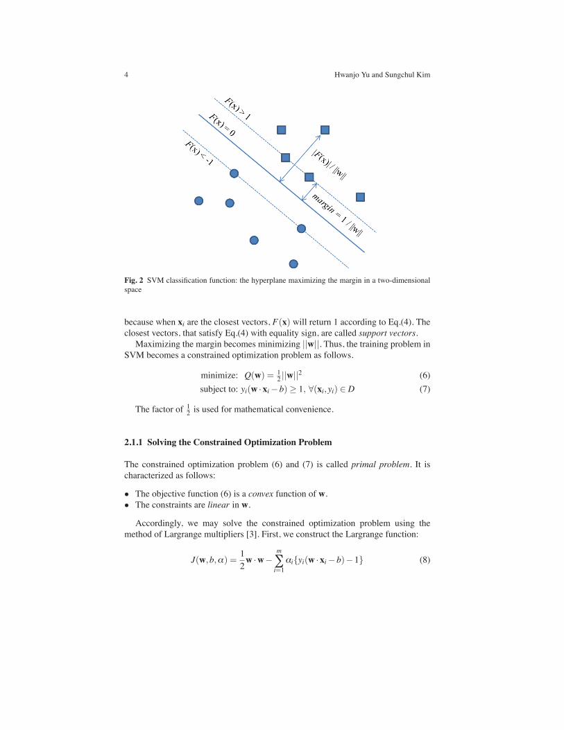
Fig. 2 SVM classification function: the hyperplane maximizing the margin in a two-dimensionalspace
because when xi are the closest vectors, F(x) will return 1 according to Eq.(4). Theclosest vectors, that satisfy Eq.(4) with equality sign, are called support vectors.Maximizing the margin becomes minimizing ||w||. Thus, the training problem in
SVM becomes a constrained optimization problem as follows.
minimize: Q(w) = 12 ||w||
2 (6)subject to: yi(w ·xi−b) ≥ 1, ∀(xi,yi) ∈ D (7)
The factor of 12 is used for mathematical convenience.
2.1.1 Solving the Constrained Optimization Problem
The constrained optimization problem (6) and (7) is called primal problem. It ischaracterized as follows:
• The objective function (6) is a convex function of w.• The constraints are linear in w.
Accordingly, we may solve the constrained optimization problem using themethod of Largrange multipliers [3]. First, we construct the Largrange function:
J(w,b,α) =12w ·w−
m
∑i=1
αiyi(w ·xi−b)−1 (8)
SVM Tutorial: Classification, Regression, and Ranking 5
where the auxiliary nonnegative variables α are called Largrange multipliers. Thesolution to the constrained optimization problem is determined by the saddle pointof the Lagrange function J(w,b,α), which has to be minimized with respect to wand b; it also has to be maximized with respect to α . Thus, differentiating J(w,b,α)with respect to w and b and setting the results equal to zero, we get the followingtwo conditions of optimality:
Condition1 : ∂J(w,b,α)∂w = 0 (9)
Condition2 : ∂J(w,b,α)∂b = 0 (10)
After rearrangement of terms, the Condition 1 yields
w=m
∑i=1
αiyi,xi (11)
and the Condition 2 yieldsm
∑i=1
αiyi = 0 (12)
The solution vector w is defined in terms of an expansion that involves the mtraining examples.As noted earlier, the primal problem deals with a convex cost function and linear
constraints. Given such a constrained optimization problem, it is possible to con-struct another problem called dual problem. The dual problem has the same optimalvalue as the primal problem, but with the Largrange multipliers providing the opti-mal solution.To postulate the dual problem for our primal problem, we first expand Eq.(8),
term by term, as follows:
J(w,b,α) =12w ·w−
m
∑i=1
αiyiw ·xi−bm
∑i=1
αiyi+m
∑i=1
αi (13)
The third term on the right-hand side of Eq.(13) is zero by virtue of the optimalitycondition of Eq.(12). Furthermore, from Eq.(11) we have
w ·w=m
∑i=1
αiyiw ·x=m
∑i=1
m
∑j=1
αiα jyiy jxix j (14)
Accordingly, setting the objective function J(w,b,α) = Q(α), we can reformu-late Eq.(13) as
Q(α) =m
∑i=1
αi−12
m
∑i=1
m
∑j=1
αiα jyiy jxi ·x j (15)
where the αi are nonnegative.We now state the dual problem:
6 Hwanjo Yu and Sungchul Kim
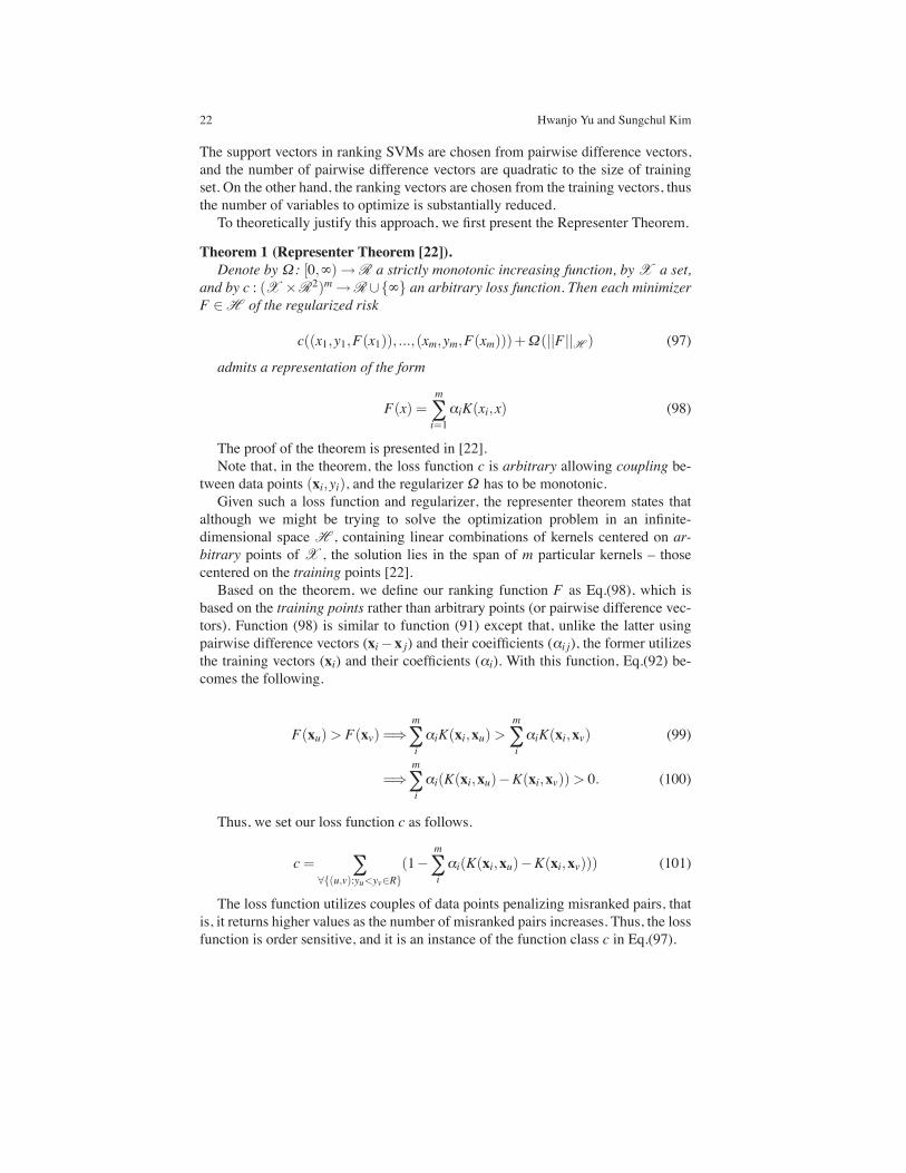
maximize: Q(α) = ∑iαi− 1
2 ∑i∑jαiα jyiy jxix j (16)
subject to: ∑iαiyi = 0 (17)
α ≥ 0 (18)
Note that the dual problem is cast entirely in terms of the training data. Moreover,the function Q(α) to be maximized depends only on the input patterns in the formof a set of dot product xi ·x jm(i, j)=1.Having determined the optimum Lagrange multipliers, denoted by α∗
i , we maycompute the optimum weight vector w∗ using Eq.(11) and so write
w∗ =∑iα∗i yixi (19)
Note that according to the property of Kuhn-Tucker conditions of optimizationtheory, The solution of the dual problem α∗
i must satisfy the following condition.
α∗i yi(w∗ ·xi−b)−1 = 0 for i= 1,2, ...,m (20)
and either α∗i or its corresponding constraint yi(w∗ ·xi−b)−1 must be nonzero.
This condition implies that only when xi is a support vector or yi(w∗ · xi− b) = 1,its corresponding coefficient αi will be nonzero (or nonnegative from Eq.(18)). Inother words, the xi whose corresponding coefficients αi are zero will not affect theoptimum weight vector w∗ due to Eq.(19). Thus, the optimum weight vector w∗ willonly depend on the support vectors whose coefficients are nonnegative.Once we compute the nonnegative α∗
i and their corresponding suppor vectors,we can compute the bias b using a positive support vector xi from the followingequation.
b∗ = 1−w∗ ·xi (21)
The classification of Eq.(2) now becomes as follows.
F(x) =∑iαiyixi ·x−b (22)
2.2 Soft-margin SVM Classification
The discussion so far has focused on linearly separable cases. However, the opti-mization problem (6) and (7) will not have a solution if D is not linearly separable.To deal with such cases, soft margin SVM allows mislabeled data points while stillmaximizing the margin. The method introduces slack variables, ξi, which measure
SVM Tutorial: Classification, Regression, and Ranking 7
the degree of misclassification. The following is the optimization problem for softmargin SVM.
minimize: Q1(w,b,ξi) = 12 ||w||
2+C∑iξi (23)
subject to: yi(w ·xi−b) ≥ 1−ξi, ∀(xi,yi) ∈ D (24)ξi ≥ 0 (25)
Due to the ξi in Eq.(24), data points are allowed to be misclassified, and theamount of misclassification will be minimized while maximizing the margin ac-cording to the objective function (23). C is a parameter that determines the tradeoffbetween the margin size and the amount of error in training.Similarily to the case of hard-margin SVM, this primal form can be transformed
to the following dual form using the Lagrange multipliers.
maximize: Q2(α) = ∑iαi−∑
i∑jαiα jyiy jxix j (26)
subject to: ∑iαiyi = 0 (27)
C ≥ α ≥ 0 (28)
Note that neither the slack variables ξi nor their Lagrange multipliers appear inthe dual problem. The dual problem for the case of nonseparable patterns is thussimilar to that for the simple case of linearly separable patterns except for a minorbut important difference. The objective function Q(α) to be maximized is the samein both cases. The nonseparable case differs from the separable case in that theconstraint αi ≥ 0 is replaced with the more stringent constraint C ≥ αi ≥ 0. Exceptfor this modification, the constrained optimization for the nonseparable case andcomputations of the optimum values of the weight vector w and bias b proceed inthe same way as in the linearly separable case.Just as the hard-margin SVM, α constitute a dual representation for the weight
vector such thatw∗ =
ms∑i=1
α∗i yixi (29)
where ms is the number of support vectors whose corresponding coefficient αi > 0.The determination of the optimum values of the bias also follows a procedure similarto that described before. Once α and b are computed, the function Eq.(22) is usedto classify new object.We can further disclose relationships among α , ξ , and C by the Kuhn-Tucker
conditions which are defined by
αiyi(w ·xi−b)−1+ξi = 0, i= 1,2, ...,m (30)
and
8 Hwanjo Yu and Sungchul Kim
µiξi = 0, i= 1,2, ...,m (31)
Eq.(30) is a rewrite of Eq.(20) except for the replacement of the unity term (1−ξi). As for Eq.(31), the µi are Lagrange multipliers that have been introduced toenforce the nonnegativity of the slack variables ξi for all i. At the saddle point thederivative of the Lagrange function for the primal problem with respect to the slackvariable ξi is zero, the evaluation of which yields
αi+µi =C (32)
By combining Eqs.(31) and (32), we see that
ξi = 0 if αi <C, and (33)ξi ≥ 0 if αi =C (34)
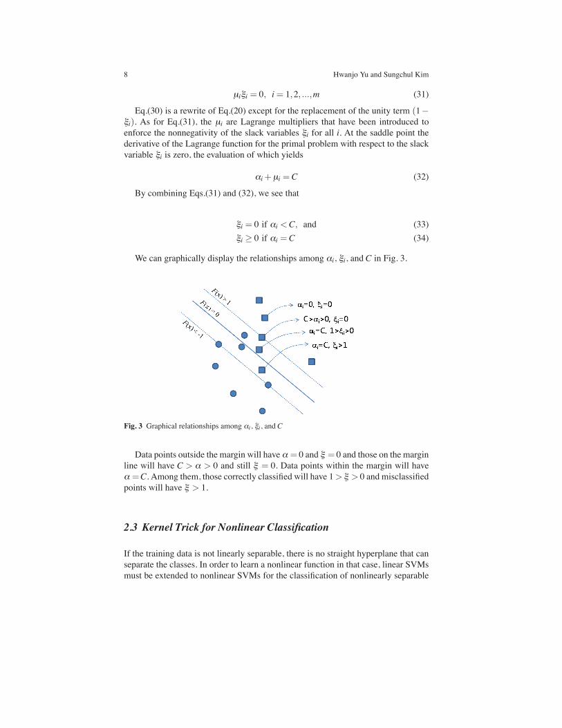
We can graphically display the relationships among αi, ξi, and C in Fig. 3.
Fig. 3 Graphical relationships among αi, ξi, and C
Data points outside the margin will have α = 0 and ξ = 0 and those on the marginline will have C > α > 0 and still ξ = 0. Data points within the margin will haveα =C. Among them, those correctly classified will have 1> ξ > 0 and misclassifiedpoints will have ξ > 1.
2.3 Kernel Trick for Nonlinear Classification
If the training data is not linearly separable, there is no straight hyperplane that canseparate the classes. In order to learn a nonlinear function in that case, linear SVMsmust be extended to nonlinear SVMs for the classification of nonlinearly separable

SVM Tutorial: Classification, Regression, and Ranking 9
data. The process of finding classification functions using nonlinear SVMs consistsof two steps. First, the input vectors are transformed into high-dimensional featurevectors where the training data can be linearly separated. Then, SVMs are used tofind the hyperplane of maximal margin in the new feature space. The separating hy-perplane becomes a linear function in the transformed feature space but a nonlinearfunction in the original input space.Let x be a vector in the n-dimensional input space and ϕ(·) be a nonlinear map-
ping function from the input space to the high-dimensional feature space. The hyper-plane representing the decision boundary in the feature space is defined as follows.
w ·ϕ(x)−b= 0 (35)
where w denotes a weight vector that can map the training data in the high dimen-sional feature space to the output space, and b is the bias. Using the ϕ(·) function,the weight becomes
w=∑αiyiϕ(xi) (36)
The decision function of Eq.(22) becomes
F(x) =m
∑iαiyiϕ(xi) ·ϕ(x)−b (37)
Furthermore, the dual problem of soft-margin SVM (Eq.(26)) can be rewrittenusing the mapping function on the data vectors as follows.
Q(α) =∑iαi−
12∑i ∑j
αiα jyiy jϕ(xi) ·ϕ(x j) (38)
holding the same constraints.Note that the feature mapping functions in the optimization problem and also in
the classifying function always appear as dot products, e.g., ϕ(xi) ·ϕ(x j). ϕ(xi) ·ϕ(x j) is the inner product between pairs of vectors in the transformed feature space.Computing the inner product in the transformed feature space seems to be quitecomplex and suffer from the curse of dimensionality problem. To avoid this prob-lem, the kernel trick is used. The kernel trick replaces the inner product in the featurespace with a kernel function K in the original input space as follows.
K(u,v) = ϕ(u) ·ϕ(v) (39)
The Mercer’s theorem proves that a kernel function K is valid, if and only if, thefollowing conditions are satisfied, for any function ψ(x). (Refer to [9] for the proofin detail.)
∫
K(u,v)ψ(u)ψ(v)dxdy≤ 0 (40)
where∫
ψ(x)2dx≤ 0
10 Hwanjo Yu and Sungchul Kim
The Mercer’s theorem ensures that the kernel function can be always expressedas the inner product between pairs of input vectors in some high-dimensional space,thus the inner product can be calculated using the kernel function only with inputvectors in the original space without transforming the input vectors into the high-dimensional feature vectors.The dual problem is now defined using the kernel function as follows.
maximize: Q2(α) = ∑iαi−∑
i∑jαiα jyiy jK(xi,x j) (41)
subject to: ∑iαiyi = 0 (42)
C ≥ α ≥ 0 (43)
The classification function becomes:
F(x) =∑iαiyiK(xi,x)−b (44)
Since K(·) is computed in the input space, no feature transformation will be ac-tually done or no ϕ(·) will be computed, and thus the weight vector w=∑αiyiϕ(x)will not be computed either in nonlinear SVMs.The followings are popularly used kernel functions.
• Polynomial: K(a,b) = (a ·b+1)d• Radial Basis Function (RBF): K(a,b) = exp(−γ||a−b||2)• Sigmoid: K(a,b) = tanh(κa ·b+ c)
Note that, the kernel function is a kind of similarity function between two vectorswhere the function output is maximized when the two vectors become equivalent.Because of this, SVM can learn a function from any shapes of data beyond vectors(such as trees or graphs) as long as we can compute a similarity function betweenany pairs of data objects. Further discussions on the properties of these kernel func-tions are out of the scope. We will instead give an example of using polynomialkernel for learning an XOR function in the following section.
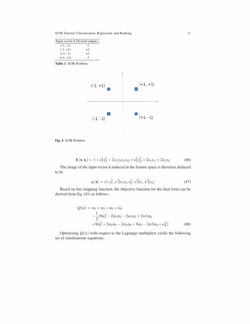
2.3.1 Example: XOR problem
To illustrate the procedure of training a nonlinear SVM function, assume we aregiven a training set of Table 1.Figure 4 plots the training points in the 2-D input space. There is no linear func-
tion that can separate the training points.To proceed, let
K(x,xi) = (1+x ·xi)2 (45)
If we denote x = (x1,x2) and xi = (xi1,xi2), the kernel function is expressed interms of monomials of various orders as follows.
iphxer
SVM Tutorial: Classification, Regression, and Ranking 11
Input vector x Desired output y(-1, -1) -1(-1, +1) +1(+1, -1) +1(+1, +1) -1
Table 1 XOR Problem
Fig. 4 XOR Problem
K(x,xi) = 1+ x21x2i1+2x1x2xi1xi2+ x22x2i2+2x1xi1+2x2xi2 (46)
The image of the input vector x induced in the feature space is therefore deducedto be
ϕ(x) = (1,x21,√2x1x2,x22,
√2x1,
√2x2) (47)
Based on this mapping function, the objective function for the dual form can bederived from Eq. (41) as follows.
Q(α) = α1+α2+α3+α4
−12(9α21 −2α1α2−2α1α3+2α1α4
+9α22 +2α2α3−2α2α4+9α3−2α3α4+α24 ) (48)
Optimizing Q(α) with respect to the Lagrange multipliers yields the followingset of simultaneous equations:
12 Hwanjo Yu and Sungchul Kim
9α1−α2−α3+α4 = 1−α1+9α2+α3−α4 = 1−α1+α2+9α3−α4 = 1α1−α2−α3+9α4 = 1
Hence, the optimal values of the Lagrange multipliers are
α1 = α2 = α3 = α4 = 18
This result denotes that all four input vectors are support vectors and the optimumvalue of Q(α) is
Q(α) = 14
and
12||w||2 =
14, or ||w|| =
1√2
From Eq.(36), we find that the optimum weight vector is
w =18[−ϕ(x1)+ϕ(x2)+ϕ(x3)−ϕ(x4)]
=18
⎡
⎢
⎢
⎢
⎢
⎢
⎢
⎣
−
⎡
⎢
⎢
⎢
⎢
⎢
⎢
⎣
11√2
1−√2
−√2
⎤
⎥
⎥
⎥
⎥
⎥
⎥
⎦
+
⎡
⎢
⎢
⎢
⎢
⎢
⎢
⎣
11−√2
1−√2√
2
⎤
⎥
⎥
⎥
⎥
⎥
⎥
⎦
+
⎡
⎢
⎢
⎢
⎢
⎢
⎢
⎣
11−√2
1√2
−√2
⎤
⎥
⎥
⎥
⎥
⎥
⎥
⎦
−
⎡
⎢
⎢
⎢
⎢
⎢
⎢
⎣
11√2
1√2√2
⎤
⎥
⎥
⎥
⎥
⎥
⎥
⎦
⎤
⎥
⎥
⎥
⎥
⎥
⎥
⎦
=
⎡
⎢
⎢
⎢
⎢
⎢
⎢
⎣
00− 1√
2000
⎤
⎥
⎥
⎥
⎥
⎥
⎥
⎦
(49)
The bias b is 0 because the first element of w is 0. The optimal hyperplane be-comes
w ·ϕ(x) = [0 0−1√2
0 0 0]
⎡
⎢
⎢
⎢
⎢
⎢
⎢
⎣
1x21√2x1x2
x22√2x1√22
⎤
⎥
⎥
⎥
⎥
⎥
⎥
⎦
= 0 (50)
which reduces to
−x1x2 = 0 (51)
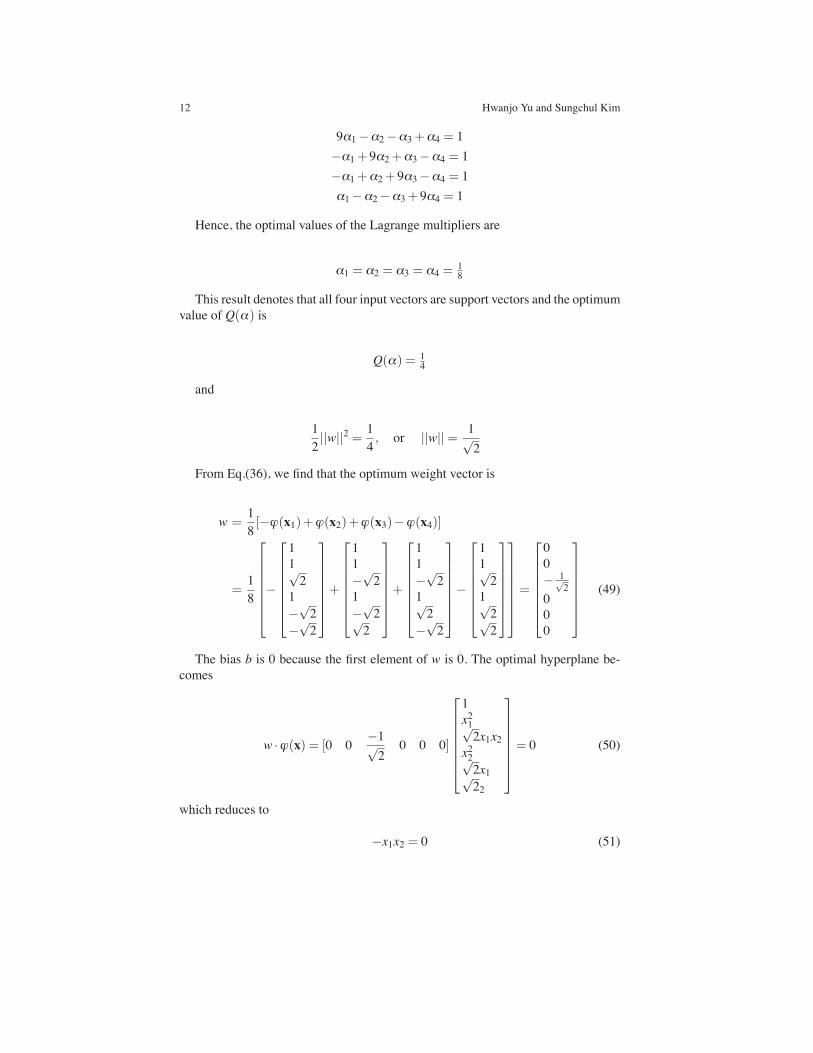
SVM Tutorial: Classification, Regression, and Ranking 13
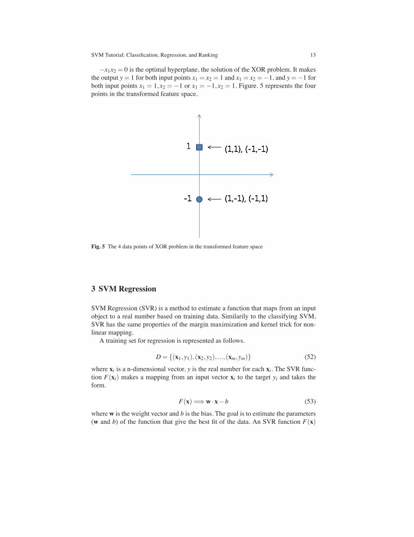
−x1x2 = 0 is the optimal hyperplane, the solution of the XOR problem. It makesthe output y= 1 for both input points x1 = x2 = 1 and x1 = x2 =−1, and y=−1 forboth input points x1 = 1,x2 = −1 or x1 = −1,x2 = 1. Figure. 5 represents the fourpoints in the transformed feature space.
Fig. 5 The 4 data points of XOR problem in the transformed feature space
3 SVM Regression
SVM Regression (SVR) is a method to estimate a function that maps from an inputobject to a real number based on training data. Similarily to the classifying SVM,SVR has the same properties of the margin maximization and kernel trick for non-linear mapping.A training set for regression is represented as follows.
D= (x1,y1),(x2,y2), ...,(xm,ym) (52)
where xi is a n-dimensional vector, y is the real number for each xi. The SVR func-tion F(xi) makes a mapping from an input vector xi to the target yi and takes theform.
F(x) =⇒ w ·x−b (53)
wherew is the weight vector and b is the bias. The goal is to estimate the parameters(w and b) of the function that give the best fit of the data. An SVR function F(x)
14 Hwanjo Yu and Sungchul Kim
approximates all pairs (xi, yi) while maintaining the differences between estimatedvalues and real values under ε precision. That is, for every input vector x in D,
yi−w ·xi−b≤ ε (54)w ·xi+b− yi ≤ ε (55)
The margin is
margin=1
||w|| (56)
By minimizing ||w||2 to maximize the margin, the training in SVR becomes aconstrained optimization problem as follows.
minimize: L(w) = 12 ||w||
2 (57)subject to: yi−w ·xi−b≤ ε (58)
w ·xi+b− yi ≤ ε (59)
The solution of this problem does not allow any errors. To allow some errors todeal with noise in the training data, The soft margin SVR uses slack variables ξ andξ . Then, the optimization problem can be revised as follows.
minimize: L(w,ξ ) = 12 ||w||
2+C∑i(ξ 2i , ξ 2i ), C > 0 (60)
subject to: yi−w ·xi−b≤ ε+ξi, ∀(xi,yi) ∈ D (61)w ·xi+b− yi ≤ ε+ ξi, ∀(xi,yi) ∈ D (62)
ξ , ξi ≥ 0 (63)
The constant C > 0 is the trade-off parameter between the margin size and theamount of errors. The slack variables ξ and ξ deal with infeasible constraints of theoptimization problem by imposing the penalty to the excess deviations which arelarger than ε .To solve the optimization problem Eq.(60), we can construct a Lagrange function
from the objective function with Lagrange multipliers as follows:
SVM Tutorial: Classification, Regression, and Ranking 15
minimize: L= 12 ||w||
2+C∑i(ξi+ ξi)−∑
i(ηiξi+ ηiξi) (64)
−∑iαi(ε+ηi− yi+w ·xi+b)
−∑iαi(ε+ ηi+ yi−w ·xi−b)
subject to: η , ηi ≥ 0 (65)α, αi ≥ 0 (66)
where ηi, ηi,α, αi are the Lagrange multipliers which satisfy positive constraints.The following is the process to find the saddle point by using the partial derivativesof L with respect to each lagrangian multipliers for minimizing the function L.
∂L∂b
=∑i(αi− αi) = 0 (67)
∂L∂w = w−Σ(αi− αi)xi = 0,w=∑
i(αi− αi)xi (68)
∂L∂ ξi
= C− αi− ηi = 0, ηi =C− αi (69)
The optimization problem with inequality constraints can be changed to follow-ing dual optimization problem by substituting Eq. (67), (68) and (69) into (64).
maximize: L(α) = ∑iyi(αi− αi)− ε ∑
i(αi+ αi) (70)
− 12 ∑i
∑j(αi− αi)(αi− αi)xix j (71)
subject to: ∑i(αi− αi) = 0 (72)
0≤ α, α ≤C (73)
The dual variables η , ηi are eliminated in revising Eq. (64) into Eq. (70). Eq. (68)and (68) can be rewritten as follows.
w =∑i(αi− αi)xi (74)
ηi = C−αi (75)ηi = C− αi (76)
where w is represented by a linear combination of the training vectors xi. Accord-ingly, the SVR function F(x) becomes the following function.
F(x) =⇒∑i(αi− αi)xix+b (77)
16 Hwanjo Yu and Sungchul Kim
Eq.(77) can map the training vectors to target real values with allowing someerrors but it cannot handle the nonlinear SVR case. The same kernel trick can beapplied by replacing the inner product of two vectors xi,x j with a kernel functionK(xi,x j). The transformed feature space is usually high dimensional, and the SVRfunction in this space becomes nonlinear in the original input space. Using the kernelfunction K, The inner product in the transformed feature space can be computed asfast as the inner product xi ·x j in the original input space. The same kernel functionsintroduced in Section 2.3 can be applied here.Once replacing the original inner product with a kernel function K, the remaining
process for solving the optimization problem is very similar to that for the linearSVR. The linear optimization function can be changed by using kernel function asfollows.
maximize: L(α) = ∑iyi(αi− αi)− ε ∑
i(αi+ αi)
− 12 ∑i
∑j(αi− αi)(αi− αi)K(xi,x j) (78)
subject to: ∑i(αi− αi) = 0 (79)
αi ≥ 0,αi ≥ 0 (80)0≤ α, α ≤C (81)
Finally, the SVR function F(x) becomes the following using the kernel function.
F(x) =⇒∑i(αi−αi)K(xi,x)+b (82)
4 SVM Ranking
Ranking SVM, learning a ranking (or preference) function, has produced variousapplications in information retrieval [14, 16, 28]. The task of learning ranking func-tions is distinguished from that of learning classification functions as follows:
1. While a training set in classification is a set of data objects and their class la-bels, in ranking, a training set is an ordering of data. Let “A is preferred toB” be specified as “A ≻ B”. A training set for ranking SVM is denoted asR= (x1,yi), ...,(xm,ym) where yi is the ranking of xi, that is, yi < y j if xi ≻ x j.
2. Unlike a classification function, which outputs a distinct class for a data object,a ranking function outputs a score for each data object, from which a globalordering of data is constructed. That is, the target function F(xi) outputs a scoresuch that F(xi) > F(x j) for any xi ≻ x j.
If not stated, R is assumed to be strict ordering, which means that for all pairs xiand x j in a set D, either xi ≻R x j or xi ≺R x j. However, it can be straightforwardly
SVM Tutorial: Classification, Regression, and Ranking 17
generalized to weak orderings. Let R∗ be the optimal ranking of data in which thedata is ordered perfectly according to user’s preference. A ranking function F istypically evaluated by how closely its ordering RF approximates R∗.Using the techniques of SVM, a global ranking function F can be learned from
an ordering R. For now, assume F is a linear ranking function such that:
∀(xi,x j) : yi < y j ∈ R : F(xi) > F(x j) ⇐⇒ w ·xi > w ·x j (83)
A weight vector w is adjusted by a learning algorithm. We say an orderings R islinearly rankable if there exists a function F (represented by a weight vector w) thatsatisfies Eq.(83) for all (xi,x j) : yi < y j ∈ R.The goal is to learn F which is concordant with the ordering R and also generalize
well beyond R. That is to find the weight vector w such that w ·xi > w ·x j for mostdata pairs (xi,x j) : yi < y j ∈ R.Though this problem is known to be NP-hard [10], The solution can be approxi-
mated using SVM techniques by introducing (non-negative) slack variables ξi j andminimizing the upper bound ∑ξi j as follows [14]:
minimize: L1(w,ξi j) = 12w ·w+C∑ξi j (84)
subject to: ∀(xi,x j) : yi < y j ∈ R : w ·xi ≥ w ·x j +1−ξi j (85)∀(i, j) : ξi j ≥ 0 (86)
By the constraint (85) and by minimizing the upper bound∑ξi j in (84), the aboveoptimization problem satisfies orderings on the training set R with minimal error.By minimizing w ·w or by maximizing the margin (= 1
||w|| ), it tries to maximize thegeneralization of the ranking function. We will explain how maximizing the margincorresponds to increasing the generalization of ranking in Section 4.1. C is the softmargin parameter that controls the trade-off between the margin size and trainingerror.By rearranging the constraint (85) as
w(xi−x j) ≥ 1−ξi j (87)
The optimization problem becomes equivalent to that of classifying SVM on pair-wise difference vectors (xi−x j). Thus, we can extend an existing SVM implemen-tation to solve the problem.Note that the support vectors are the data pairs (xsi ,xsj) such that constraint (87)
is satisfied with the equality sign, i.e., w(xsi − xsj) = 1− ξi j. Unbounded supportvectors are the ones on the margin (i.e., their slack variables ξi j = 0), and boundedsupport vectors are the ones within the margin (i.e., 1> ξi j > 0) or misranked (i.e.,ξi j > 1). As done in the classifying SVM, a function F in ranking SVM is alsoexpressed only by the support vectors.Similarily to the classifying SVM, the primal problem of ranking SVM can be
transformed to the following dual problem using the Lagrange multipliers.
iphxer
18 Hwanjo Yu and Sungchul Kim
maximize: L2(α) = ∑i jαi j−∑
i j∑uvαi jαuvK(xi−x j,xu−xv) (88)
subject to: C ≥ α ≥ 0 (89)
Once transformed to the dual, the kernel trick can be applied to support nonlin-ear ranking function. K(·) is a kernel function. αi j is a coefficient for a pairwisedifference vectors (xi−x j). Note that the kernel function is computed for P2(∼m4)times where P is the number of data pairs and m is the number of data points inthe training set, thus solving the ranking SVM takes O(m4) at least. Fast trainingalgorithms for ranking SVM have been proposed [17] but they are limited to linearkernels.Once α is computed, w can be written in terms of the pairwise difference vectors
and their coefficients such that:
w=∑i jαi j(xi−x j) (90)
The ranking function F on a new vector z can be computed using the kernelfunction replacing the dot product as follows:
F(z) = w · z=∑i jαi j(xi−x j) · z=∑
i jαi jK(xi−x j,z). (91)
4.1 Margin-Maximization in Ranking SVM
Fig. 6 Linear projection of four data points
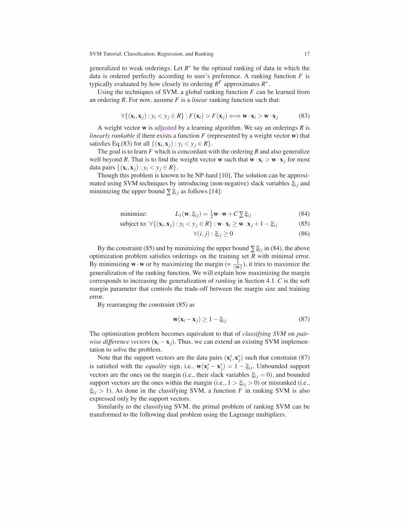
We now explain the margin-maximization of the ranking SVM, to reason abouthow the ranking SVM generates a ranking function of high generalization. We firstestablish some essential properties of ranking SVM. For convenience of explana-
SVM Tutorial: Classification, Regression, and Ranking 19
tion, we assume a training set R is linearly rankable and thus we use hard-marginSVM, i.e., ξi j = 0 for all (i, j) in the objective (84) and the constraints (85).In our ranking formulation, from Eq.(83), the linear ranking function Fw projects
data vectors onto a weight vectorw. For instance, Fig. 6 illustrates linear projectionsof four vectors x1,x2,x3,x4 onto two different weight vectors w1 and w2 respec-tively in a two-dimensional space. Both Fx1 and Fx2 make the same ordering R forthe four vectors, that is, x1 >R x2 >R x3 >R x4. The ranking difference of two vec-tors (xi,x j) according to a ranking function Fw is denoted by the geometric distanceof the two vectors projected onto w, that is, formulated as w(xi−x j)
||w|| .
Corollary 1. Suppose Fw is a ranking function computed by the hard-margin rank-ing SVM on an ordering R. Then, the support vectors of Fw represent the data pairsthat are closest to each other when projected to w thus closest in ranking.
Proof. The support vectors are the data pairs (xsi ,xsj) such that w(xsi − xsj) = 1 inconstraint (87), which is the smallest possible value for all data pairs ∀(xi,x j) ∈ R.Thus, its ranking difference according to Fw(=
w(xsi−xsj)
||w|| ) is also the smallest amongthem [24].
Corollary 2. The ranking function F, generated by the hard-margin ranking SVM,maximizes the minimal difference of any data pairs in ranking.
Proof. By minimizing w ·w, the ranking SVM maximizes the margin δ = 1||w|| =
w(xsi−xsj)
||w|| where (xsi ,xsj) are the support vectors, which denotes, from the proof ofCorollary 1, the minimal difference of any data pairs in ranking.
The soft margin SVM allows bounded support vectors whose ξi j > 0 as well asunbounded support vectors whose ξi j = 0, in order to deal with noise and allowsmall error for the R that is not completely linearly rankable. However, the objectivefunction in (84) also minimizes the amount of the slacks and thus the amount oferror, and the support vectors are the close data pairs in ranking. Thus, maximizingthe margin generates the effect of maximizing the differences of close data pairs inranking.From Corollary 1 and 2, we observe that ranking SVM improves the general-
ization performance by maximizing the minimal ranking difference. For example,consider the two linear ranking functions Fw1 and Fw2 in Fig. 6. Although the twoweight vectors w1 and w2 make the same ordering, intuitively w1 generalizes betterthan w2 because the distance between the closest vectors on w1 (i.e., δ1) is largerthan that on w2 (i.e., δ2). SVM computes the weight vector w that maximizes thedifferences of close data pairs in ranking. Ranking SVMs find a ranking function ofhigh generalization in this way.
20 Hwanjo Yu and Sungchul Kim
5 Ranking Vector Machine: An Efficient Method for Learningthe 1-norm Ranking SVM
This section presents another rank learning method, Ranking Vector Machine (RVM),a revised 1-norm ranking SVM that is better for feature selectoin and more scalableto large data sets than the standard ranking SVM.We first develop a 1-norm ranking SVM, a ranking SVM that is based on 1-norm
objective function. (The standard ranking SVM is based on 2-norm objective func-tion.) The 1-norm ranking SVM learns a function with much less support vectorsthan the standard SVM. Thereby, its testing time is much faster than 2-norm SVMsand provides better feature selection properties. (The function of 1-norm SVM islikely to utilize a less number of features by using a less number of support vec-tors [11].) Feature selection is also important in ranking. Ranking functions are rele-vance or preference functions in document or data retrieval. Identifying key featuresincreases the interpretability of the function. Feature selection for nonlinear kernelis especially challenging, and the fewer the number of support vectors are, the moreefficiently feature selection can be done [12, 20, 6, 30, 8].We next present RVM which revises the 1-norm ranking SVM for fast training.
The RVM trains much faster than standard SVMs while not compromising the ac-curacy when the training set is relatively large. The key idea of RVM is to express theranking function with “ranking vectors” instead of support vectors. Support vectorsin ranking SVMs are pairwise difference vectors of the closest pairs as discussed inSection 4. Thus, the training requires investigating every data pair as potential can-didates of support vectors, and the number of data pairs are quadratic to the size oftraining set. On the other hand, the ranking function of the RVM utilizes each train-ing data object instead of data pairs. Thus, the number of variables for optimizationis substantially reduced in the RVM.
5.1 1-norm Ranking SVM
The goal of 1-norm ranking SVM is the same as that of the standard ranking SVM,that is, to learn F that satisfies Eq.(83) for most (xi,x j) : yi < y j ∈R and generalizewell beyond the training set. In the 1-norm ranking SVM, we express Eq.(83) usingthe F of Eq.(91) as follows.
F(xu) > F(xv) =⇒P
∑i jαi j(xi−x j) ·xu >
P
∑i jαi j(xi−x j) ·xv (92)
=⇒P
∑i jαi j(xi−x j) · (xu−xv) > 0 (93)
Then, replacing the inner product with a kernel function, the 1-norm rankingSVM is formulated as:

SVM Tutorial: Classification, Regression, and Ranking 21
minimize : L(α,ξ ) =P∑i jαi j +C
P∑i jξi j (94)
s.t. :P∑i jαi jK(xi−x j,xu−xv) ≥ 1−ξuv, ∀(u,v) : yu < yv ∈ R (95)
α ≥ 0, ξ ≥ 0 (96)
While the standard ranking SVM suppresses the weight w to improve the gener-alization performance, the 1-norm ranking suppresses α in the objective function.Since the weight is expressed by the sum of the coefficient times pairwise rank-ing difference vectors, suppressing the coefficient α corresponds to suppressing theweight w in the standard SVM. (Mangasarian proves it in [18].)C is a user parame-ter controlling the tradeoff between the margin size and the amount of error, ξ , andK is the kernel function. P is the number of pairwise difference vectors (∼ m2).The training of the 1-norm ranking SVM becomes a linear programming (LP)
problem thus solvable by LP algorithms such as the Simplex and Interior Pointmethod [18, 11, 19]. Just as the standard ranking SVM, K needs to be computed P2(∼m4) times, and there are P number of constraints (95) and α to compute. Once αis computed, F is computed using the same ranking function as the standard rankingSVM, i.e., Eq.(91).The accuracies of 1-norm ranking SVM and standard ranking SVM are compara-
ble, and both methods need to compute the kernel functionO(m4) times. In practice,the training of the standard SVM is more efficient because fast decomposition al-gorithms have been developed such as sequential minimal optimization (SMO) [21]while the 1-norm ranking SVM uses common LP solvers.It is shown that 1-norm SVMs use much less support vectors that standard 2-
norm SVMs, that is, the number of positive coefficients (i.e., α > 0) after trainingis much less in the 1-norm SVMs than in the standard 2-norm SVMs [19, 11]. Itis because, unlike the standard 2-norm SVM, the support vectors in the 1-normSVM are not bounded to those close to the boundary in classification or the minimalranking difference vectors in ranking. Thus, the testing involves much less kernelevaluations, and it is more robust when the training set contains noisy features [31].
5.2 Ranking Vector Machine
Although the 1-norm ranking SVM has merits over the standard ranking SVM interms of the testing efficiency and feature selection, its training complexity is veryhigh w.r.t. the number of data points. In this section, we present Ranking VectorMachine (RVM), which revises the 1-norm ranking SVM to reduce the trainingtime substantially. The RVM significantly reduces the number of variables in theoptimization problem while not compromizing the accuracy. The key idea of RVMis to express the ranking function with “ranking vectors” instead of support vectors.
22 Hwanjo Yu and Sungchul Kim
The support vectors in ranking SVMs are chosen from pairwise difference vectors,and the number of pairwise difference vectors are quadratic to the size of trainingset. On the other hand, the ranking vectors are chosen from the training vectors, thusthe number of variables to optimize is substantially reduced.To theoretically justify this approach, we first present the Representer Theorem.
Theorem 1 (Representer Theorem [22]).Denote by Ω : [0,∞) → R a strictly monotonic increasing function, by X a set,
and by c : (X ×R2)m → R∪∞ an arbitrary loss function. Then each minimizerF ∈ H of the regularized risk
c((x1,y1,F(x1)), ...,(xm,ym,F(xm)))+Ω(||F||H ) (97)
admits a representation of the form
F(x) =m
∑i=1
αiK(xi,x) (98)
The proof of the theorem is presented in [22].Note that, in the theorem, the loss function c is arbitrary allowing coupling be-
tween data points (xi,yi), and the regularizer Ω has to be monotonic.Given such a loss function and regularizer, the representer theorem states that
although we might be trying to solve the optimization problem in an infinite-dimensional space H , containing linear combinations of kernels centered on ar-bitrary points of X , the solution lies in the span of m particular kernels – thosecentered on the training points [22].Based on the theorem, we define our ranking function F as Eq.(98), which is
based on the training points rather than arbitrary points (or pairwise difference vec-tors). Function (98) is similar to function (91) except that, unlike the latter usingpairwise difference vectors (xi−x j) and their coeifficients (αi j), the former utilizesthe training vectors (xi) and their coefficients (αi). With this function, Eq.(92) be-comes the following.
F(xu) > F(xv) =⇒m
∑iαiK(xi,xu) >
m
∑iαiK(xi,xv) (99)
=⇒m
∑iαi(K(xi,xu)−K(xi,xv)) > 0. (100)
Thus, we set our loss function c as follows.
c= ∑∀(u,v):yu<yv∈R
(1−m
∑iαi(K(xi,xu)−K(xi,xv))) (101)
The loss function utilizes couples of data points penalizing misranked pairs, thatis, it returns higher values as the number of misranked pairs increases. Thus, the lossfunction is order sensitive, and it is an instance of the function class c in Eq.(97).
SVM Tutorial: Classification, Regression, and Ranking 23
We set the regularizerΩ(|| f ||H ) =m∑iαi (αi≥ 0), which is strictly monotonically
increasing. Let P is the number of pairs (u,v) ∈ R such that yu < yv, and let ξuv =
1−m∑iαi(K(xi,xu)−K(xi,xv)). Then, our RVM is formulated as follows.
minimize: L(α,ξ ) =m∑iαi+C
P∑i jξi j (102)
s.t.:m∑iαi(K(xi,xu)−K(xi,xv)) ≥ 1−ξuv,∀(u,v) : yu < yv ∈ R (103)
α,ξ ≥ 0 (104)
The solution of the optimization problem lies in the span of kernels centered onthe training points (i.e., Eq.(98)) as suggested in the representer theorem. Just asthe 1-norm ranking SVM, the RVM suppresses α to improve the generalization,and forces Eq.(100) by constraint (103). Note that there are only m number of αiin the RVM. Thus, the kernel function is evaluated O(m3) times while the standardranking SVM computes it O(m4) times.Another rationale of RVM or rationale of using training vectors instead of pair-
wise difference vectors in the ranking function is that the support vectors in the1-norm ranking SVM are not the closest pairwise difference vectors, thus express-ing the ranking function with pairwise difference vectors becomes not as beneficialin the 1-norm ranking SVM. To explain this further, consider classifying SVMs. Un-like the 2-norm (classifying) SVM, the support vectors in the 1-norm (classifying)SVM are not limited to those close to the decision boundary. This makes it possi-ble that the 1-norm (classifying) SVM can express the similar boundary functionwith less number of support vectors. Directly extended from the 2-norm (classify-ing) SVM, the 2-norm ranking SVM improves the generalization by maximizingthe closest pairwise ranking difference that corresponds to the margin in the 2-norm(classifying) SVM as discussed in Section 4. Thus, the 2-norm ranking SVM ex-presses the function with the closest pairwise difference vectors (i.e., the supportvectors). However, the 1-norm ranking SVM improves the generalization by sup-pressing the coefficients α just as the 1-norm (classifying) SVM. Thus, the supportvectors in the 1-norm ranking SVM are not the closest pairwise difference vectorsany more, and thus expressing the ranking function with pairwise difference vectorsbecomes not as beneficial in the 1-norm ranking SVM.
5.3 Experiment
This section evaluates the RVM on synthetic datasets (Section 5.3.1) and a real-world dataset (Secton 5.3.2). The RVM is compared with the state-of-the-art rank-ing SVM provided in SVM-light. Experiment results show that the RVM trainssubstantially faster than the SVM-light for nonlinear kernels while their accura-

24 Hwanjo Yu and Sungchul Kim
cies are comparable. More importantly, the number of ranking vectors in the RVMis multiple orders of magnitudes smaller than the number of support vectors in theSVM-light. Experiments are performed on a Windows XP Professional machinewith a Pentium IV 2.8GHz and 1GB of RAM. We implemented the RVM usingC and used CPLEX 1 for the LP solver. The source codes are freely available at“http://iis.postech.ac.kr/rvm” [29].
Evaluation metric: MAP (mean average precision) is used to measure the rank-ing quality when there are only two classes of ranking [26], and NDCG is used toevaluate ranking performance for IR applications when there are multiple levels ofranking [2, 4, 7, 25]. Kendall’s τ is used when there is a global ordering of data andthe training data is a subset of it. Ranking SVMs as well as the RVM minimize theamount of error or mis-ranking, which is corresponding to optimizing the Kendall’sτ [16, 27]. Thus, we use the Kendall’s τ to compare their accuracy.Kendall’s τ computes the overall accuracy by comparing the similarity of two
orderings R∗ and RF . (RF is the ordering of D according to the learned function F .)The Kendall’s τ is defined based on the number of concordant pairs and discordantpairs. If R∗ and RF agree in how they order a pair, xi and x j, the pair is concordant,otherwise, it is discordant. The accuracy of function F is defined as the number ofconcordant pairs between R∗ and RF per the total number of pairs in D as follows.
F(R∗,RF) =# of concordant pairs
(
|R|2
)
For example, suppose R∗ and RF order five points x1, . . . ,x5 as follow:
(x1,x2,x3,x4,x5) ∈ R∗
(x3,x2,x1,x4,x5) ∈ RF
Then, the accuracy of F is 0.7, as the number of discordant pairs is 3, i.e.,x1,x2,x1,x3,x2,x3while all remaining 7 pairs are concordant.
5.3.1 Experiments on Synthetic Dataset
Below is the description of our experiments on synthetic datasets.
1. We randomly generated a training and a testing dataset Dtrain and Dtest respec-tively, where Dtrain contains mtrain (= 40, 80, 120, 160, 200) data points of n(e.g., 5) dimensions (i.e., mtrain-by-n matrix), and Dtest contains mtest (= 50) datapoints of n dimensions (i.e., mtest-by-n matrix). Each element in the matrices is arandom number between zero and one. (We only did experiments on the data set
1 http://www.ilog.com/products/cplex/
SVM Tutorial: Classification, Regression, and Ranking 25
0.9 0.91 0.92 0.93 0.94 0.95 0.96 0.97 0.98 0.99
1
40 60 80 100 120 140 160 180 200
Kend
all’s
tau
Size of training set
SVM (Linear)RVM (Linear)
0.9 0.91 0.92 0.93 0.94 0.95 0.96 0.97 0.98 0.99
1
40 60 80 100 120 140 160 180 200
Kend
all’s
tau
Size of training set
SVM (RBF)RVM (RBF)
(a) Linear (b) RBF
Fig. 7 Accuracy
0
2
4
6
8
10
12
40 60 80 100 120 140 160 180 200
Trai
ning
tim
e in
sec
onds
Size of training set
SVM (Linear)RVM (Linear)
0
5
10
15
20
25
30
40 60 80 100 120 140 160 180 200
Trai
ning
tim
e in
sec
onds
Size of training set
SVM (RBF)RVM (RBF)
(a) Linear Kernel (b) RBF Kernel
Fig. 8 Training time
0
50
100
150
200
40 60 80 100 120 140 160 180 200
Num
ber o
f sup
port
vect
ors
Size of training set
SVM (Linear)RVM (Linear)
0
50
100
150
200
40 60 80 100 120 140 160 180 200
Num
ber o
f sup
port
vect
ors
Size of training set
SVM (RBF)RVM (RBF)
(a) Linear Kernel (b) RBF Kernel
Fig. 9 Number of support (or ranking) vectors
of up to 200 objects due to performance reason. Ranking SVMs run intolerablyslow on data sets larger than 200.)
2. We randomly generate a global ranking function F∗, by randomly generating theweight vector w in F∗(x) = w ·x for linear, and in F∗(x) = exp(−||w−x||)2 forRBF function.
26 Hwanjo Yu and Sungchul Kim
0
0.05
0.1
0.15
0.2
0 1 2 3 4 5 6
Dec
rem
ent i
n ac
cura
cy
k
SVM (Linear)RVM (Linear)
0
0.05
0.1
0.15
0.2
0 1 2 3 4 5 6
Dec
rem
ent i
n ac
cura
cy
k
SVM (RBF)RVM (RBF)
(a) Linear (b) RBF
Fig. 10 Sensitivity to noise (mtrain = 100).
3. We rank Dtrain and Dtest according to F∗, which forms the global ordering R∗trainand R∗test on the training and testing data.
4. We train a function F from R∗train, and test the accuracy of F on R∗test .
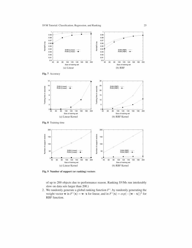
We tuned the soft margin parameter C by trying C = 10−5, 10−5, ...,105, andused the highest accuracy for comparison. For the linear and RBF functions, weused linear and RBF kernels accordingly. We repeat this entire process 30 times toget the mean accuracy.
Accuracy: Figure 7 compares the accuracies of the RVM and the ranking SVMfrom the SVM-light. The ranking SVM outperforms RVM when the size of data setis small, but their difference becomes trivial as the size of data set increases. Thisphenomenon can be explained by the fact that when the training size is too small, thenumber of potential ranking vectors becomes too small to draw an accurate rankingfunction whereas the number of potential support vectors is still large. However, asthe size of training set increases, RVM becomes as accurate as the ranking SVMbecause the number of potential ranking vectors becomes large as well.
Training Time: Figure 8 compares the training time of the RVM and the SVM-light. While the SVM light trains much faster than RVM for linear kernel (SVMlight is specially optimized for linear kernel.), the RVM trains significantly fasterthan the SVM light for RBF kernel.
Number of Support (or Ranking) Vectors: Figure 9 compares the number of sup-port (or ranking) vectors used in the function of RVM and the SVM-light. RVM’smodel uses a significantly smaller number of support vectors than the SVM-light.
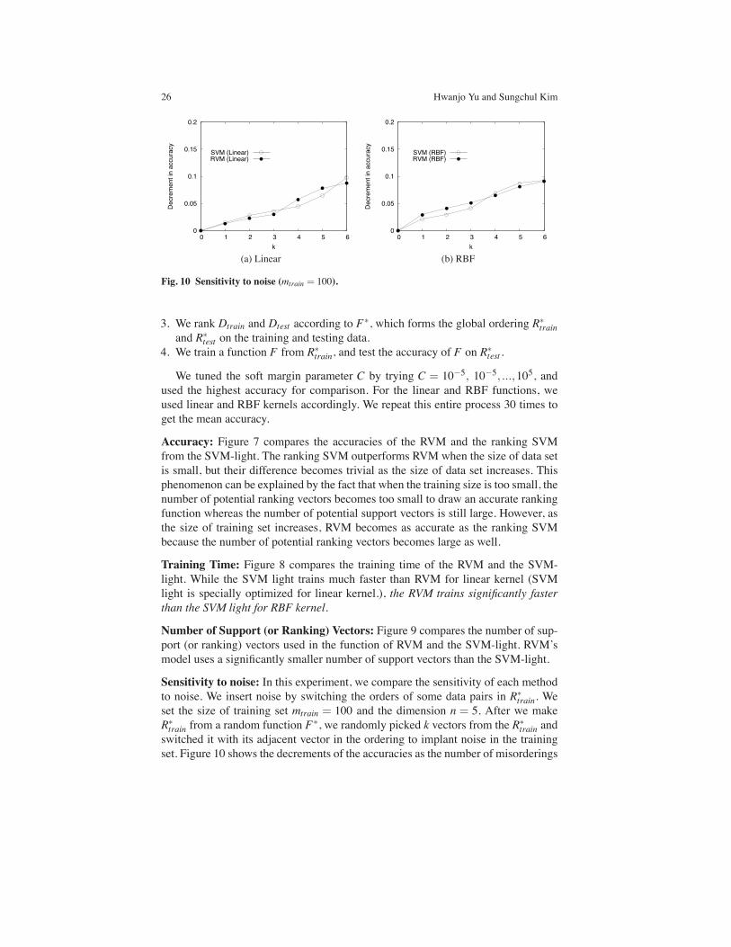
Sensitivity to noise: In this experiment, we compare the sensitivity of each methodto noise. We insert noise by switching the orders of some data pairs in R∗train. Weset the size of training set mtrain = 100 and the dimension n = 5. After we makeR∗train from a random function F∗, we randomly picked k vectors from the R∗train andswitched it with its adjacent vector in the ordering to implant noise in the trainingset. Figure 10 shows the decrements of the accuracies as the number of misorderings
SVM Tutorial: Classification, Regression, and Ranking 27
increases in the training set. Their accuracies are moderately decreasing as the noiseincreases in the training set, and their sensitivities to noise are comparable.
5.3.2 Experiment on Real Dataset
In this section, we experiment using the OHSUMED dataset obtained from theLETOR, the site containing benchmark datasets for ranking [1]. OHSUMED is acollection of documents and queries on medicine, consisting of 348,566 referencesand 106 queries. There are in total 16,140 query-document pairs upon which rel-evance judgements are made. In this dataset the relevance judgements have threelevels: “definitely relevant”, “partially relevant”, and “irrelevant”. The OHSUMEDdataset in the LETOR extracts 25 features. We report our experiments on the firstthree queries and their documents. We compare the performance of RVM and SVM-light on them. We tuned the parameters 3-fold cross validation with trying C andγ = 10−6,10−5, ...,106 for the linear and RBF kernels and compared the highestperformance. The training time is measured for training the model with the tunedparameters. We repeated the whole process three times and reported the mean val-ues.
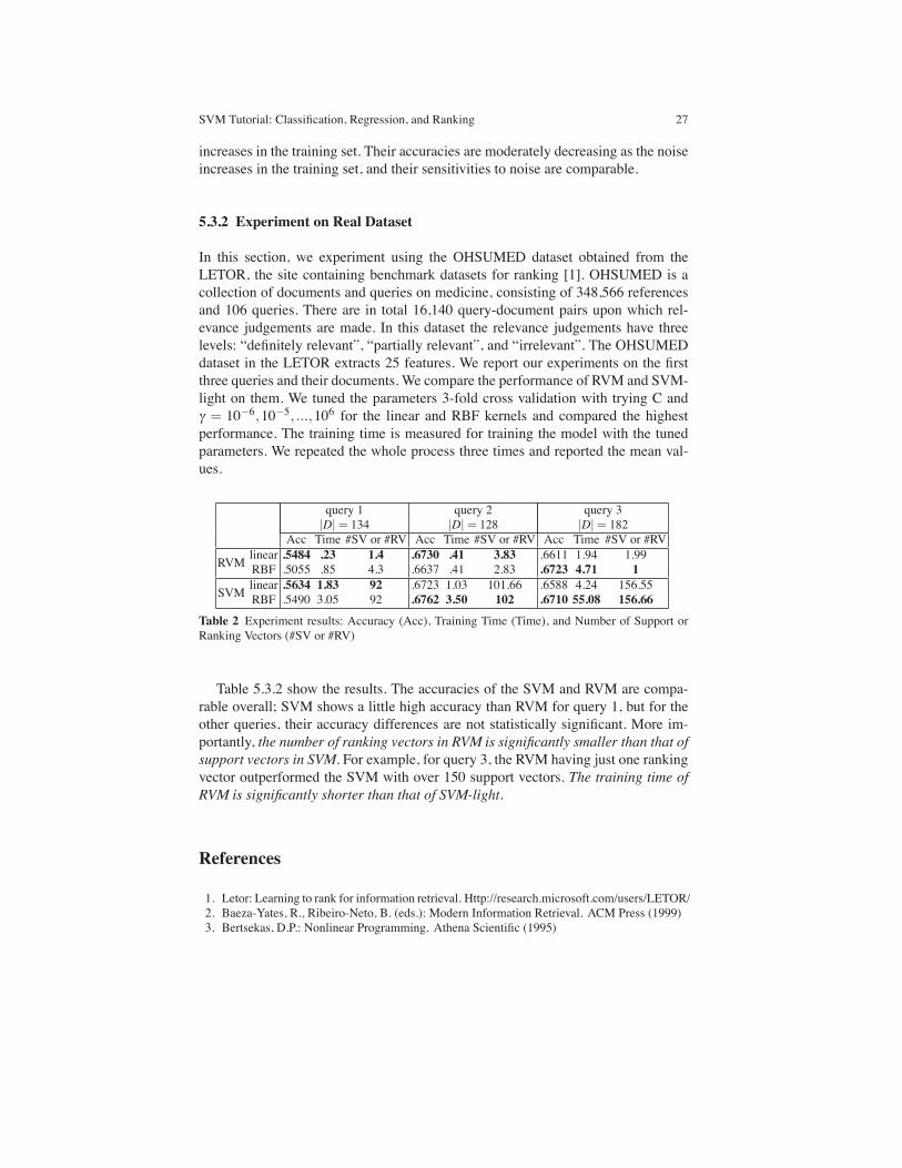
query 1 query 2 query 3|D| = 134 |D| = 128 |D| = 182
Acc Time #SV or #RV Acc Time #SV or #RV Acc Time #SV or #RVlinear .5484 .23 1.4 .6730 .41 3.83 .6611 1.94 1.99RVM RBF .5055 .85 4.3 .6637 .41 2.83 .6723 4.71 1linear .5634 1.83 92 .6723 1.03 101.66 .6588 4.24 156.55SVM RBF .5490 3.05 92 .6762 3.50 102 .6710 55.08 156.66
Table 2 Experiment results: Accuracy (Acc), Training Time (Time), and Number of Support orRanking Vectors (#SV or #RV)
Table 5.3.2 show the results. The accuracies of the SVM and RVM are compa-rable overall; SVM shows a little high accuracy than RVM for query 1, but for theother queries, their accuracy differences are not statistically significant. More im-portantly, the number of ranking vectors in RVM is significantly smaller than that ofsupport vectors in SVM. For example, for query 3, the RVM having just one rankingvector outperformed the SVM with over 150 support vectors. The training time ofRVM is significantly shorter than that of SVM-light.
References
1. Letor: Learning to rank for information retrieval. Http://research.microsoft.com/users/LETOR/2. Baeza-Yates, R., Ribeiro-Neto, B. (eds.): Modern Information Retrieval. ACM Press (1999)3. Bertsekas, D.P.: Nonlinear Programming. Athena Scientific (1995)
28 Hwanjo Yu and Sungchul Kim
4. Burges, C., Shaked, T., Renshaw, E., Lazier, A., Deeds, M., Hamilton, N., Hullender, G.:Learning to rank using gradient descent. In: Proc. Int. Conf. Machine Learning (ICML’04)(2004)
5. Burges, C.J.C.: A tutorial on support vector machines for pattern recognition. Data Miningand Knowledge Discovery 2, 121–167 (1998)
6. Cao, B., Shen, D., Sun, J.T., Yang, Q., Chen, Z.: Feature selection in a kernel space. In: Proc.Int. Conf. Machine Learning (ICML’07) (2007)
7. Cao, Y., Xu, J., Liu, T.Y., Li, H., Huang, Y., Hon, H.W.: Adapting ranking svm to documentretrieval. In: Proc. ACM SIGIR Int. Conf. Information Retrieval (SIGIR’06) (2006)
8. Cho, B., Yu, H., Lee, J., Chee, Y., Kim, I.: Nonlinear support vector machine visualizationfor risk factor analysis using nomograms and localized radial basis function kernels. IEEETransactions on Information Technology in Biomedicine ((Accepted))
9. Christianini, N., Shawe-Taylor, J.: An Introduction to support vector machines and otherkernel-based learning methods. Cambridge University Press (2000)
10. Cohen, W.W., Schapire, R.E., Singer, Y.: Learning to order things. In: Proc. Advances inNeural Information Processing Systems (NIPS’98) (1998)
11. Fung, G., Mangasarian, O.L.: A feature selection newton method for support vector machineclassification. Computational Optimization and Applications (2004)
12. Guyon, I., Elisseeff, A.: An introduction to variable and feature selection. Journal of MachineLearning Research (2003)
13. Hastie, T., Tibshirani, R.: Classification by pairwise coupling. In: Advances in Neural Infor-mation Processing Systems (1998)
14. Herbrich, R., Graepel, T., Obermayer, K. (eds.): Large margin rank boundaries for ordinalregression. MIT-Press (2000)
15. J.H.Friedman: Another approach to polychotomous classification. Tech. rep., Standford Uni-versity, Department of Statistics, 10:1895-1924 (1998)
16. Joachims, T.: Optimizing search engines using clickthrough data. In: Proc. ACM SIGKDDInt. Conf. Knowledge Discovery and Data Mining (KDD’02) (2002)
17. Joachims, T.: Training linear svms in linear time. In: Proc. ACM SIGKDD Int. Conf. Knowl-edge Discovery and Data Mining (KDD’06) (2006)
18. Mangasarian, O.L.: Generalized Support Vector Machines. MIT Press (2000)19. Mangasarian, O.L.: Exact 1-norm support vector machines via unconstrained convex differ-
entiable minimization. Journal of Machine Learning Research (2006)20. Mangasarian, O.L., Wild, E.W.: Feature selection for nonlinear kernel support vector ma-
chines. Tech. rep., University of Wisconsin, Madison (1998)21. Platt, J.: Fast training of support vector machines using sequential minimal optimization. In:
A.S. B. Scholkopf C. Burges (ed.) Advances in Kernel Methods: Support Vector Machines.MIT Press, Cambridge, MA (1998)
22. Scholkopf, B., Herbrich, R., Smola, A.J., Williamson, R.C.: A generalized representer theo-rem. In: Proc. COLT (2001)
23. Smola, A.J., Scholkopf, B.: A tutorial on support vector regression. Tech. rep., NeuroCOLT2Technical Report NC2-TR-1998-030 (1998)
24. Vapnik, V.: Statistical Learning Theory. John Wiley and Sons (1998)25. Xu, J., Li, H.: Adarank: A boosting algorithm for information retrieval. In: Proc. ACM SIGIR
Int. Conf. Information Retrieval (SIGIR’07) (2007)26. Yan, L., Dodier, R., Mozer, M.C., Wolniewicz, R.: Optimizing classifier performance via the
wilcoxon-mann-whitney statistics. In: Proc. Int. Conf. Machine Learning (ICML’03) (2003)27. Yu, H.: SVM selective sampling for ranking with application to data retrieval. In: Proc. Int.
Conf. Knowledge Discovery and Data Mining (KDD’05) (2005)28. Yu, H., Hwang, S.W., Chang, K.C.C.: Enabling soft queries for data retrieval. Information
Systems (2007)29. Yu, H., Kim, Y., Hwang, S.W.: RVM: An efficient method for learning ranking SVM. Tech.
rep., Department of Computer Science and Engineering, Pohang University of Science andTechnology (POSTECH), Pohang, Korea, http://iis.hwanjoyu.org/rvm (2008)
SVM Tutorial: Classification, Regression, and Ranking 29
30. Yu, H., Yang, J., Wang, W., Han, J.: Discovering compact and highly discriminative featuresor feature combinations of drug activities using support vector machines. In: IEEE ComputerSociety Bioinformatics Conf. (CSB’03), pp. 220–228 (2003)
31. Zhu, J., Rosset, S., Hastie, T., Tibshriani, R.: 1-norm support vector machines. In: Proc.Advances in Neural Information Processing Systems (NIPS’00) (2003)

Index
1-norm ranking SVM, 20
bias, 3binary classifier, 1binary SVMs, 2bounded support vector, 17
classification functin, 16convec function, 4curse of dimensionality problem, 9
data object, 2data point, 2dual problem, 5
feature selection, 20feature space, 2
high generalization, 18hyperplane, 9
input space, 2
Kendall’s τ , 24kernel function, 10kernel trick, 2Kuhn-Tucker conditions, 6
lagrange function, 5lagrange multiplier, 5LETOR, 27linear classifier, 2linear programming (LP) problem, 21linear ranking function, 17, 19linearly separable, 3loss function, 22LP algorithm, 21
MAP (mean average precision), 24margin, 2, 3Mercer’s theorem, 9misranked, 17multiclass classification, 1
NDCG, 24NP-hard, 17
OHSUMED, 27optimization problem, 4optimum weight vector, 6
pairwise coupling method, 1pairwise difference, 17polynomial, 10primal problem, 4
radial basis function, 10ranking diffeence, 19ranking function, 16ranking SVM, 16ranking vector machine (RVM), 21real-world dataset, 23regularizer, 22representer theorem, 22
sequential minimal optimization (SMO), 21sigmoid, 10slack variable, 6soft margin parameter, 17soft margin SVM, 6, 19standard ranking SVM, 20, 21strick ordering, 16support vector, 4SVM classification function, 3SVM regression, 13
31
32 Index
SVM-light, 23SVMs, 1SVR function, 13synthetic dataset, 23
training set, 3
unbounded support vector, 17
weight vector, 3, 9
XOR problem, 10