Sustained System Performance for HPC Systems - … › assets › RD › SSP ›...
75
W. Kramer Draft Dissertation 30 Chapter 3: Performance - Sustained System Performance for HPC Systems - The SSP Method 3.1 Chapter Summary The class of performance evaluation factors is clearly important as indicated in the analysis described in Chapter 2. This chapter explains the Sustained Systems Performance (SSP) method, which provides a process for evaluating system performance across any timeframe. SSP is a simple but powerful method in the sense that it can be applied to any set of systems, any workload and/or benchmark suite and for any time period. SSP measures time to solution across different application areas and it can be used to evaluate absolute performance and performance relative to cost (in dollars, energy or other value propositions). While the formula development in this chapter is meant to be complete, it should not be intimidating since the SSP method can be described in a straightforward explanation in Section 3.1.1 below. 3.1.1 The Basic SSP Concept SSP uses one or more benchmarks to compare the performance of two or more systems using time to solution as the primary performance indicator. Each benchmark has one or more problem sets which, together with the benchmark, determine a unique test. Each test has a total operational count (Floating Point Operations – Flops from a single reference system - are used in this work, but other operations can be
Transcript of Sustained System Performance for HPC Systems - … › assets › RD › SSP ›...

W. Kramer Draft Dissertation 30
Chapter 3: Performance - Sustained System
Performance for HPC Systems - The SSP
Method
3.1 Chapter Summary
The class of performance evaluation factors is clearly important as indicated in
the analysis described in Chapter 2. This chapter explains the Sustained Systems
Performance (SSP) method, which provides a process for evaluating system
performance across any timeframe. SSP is a simple but powerful method in the sense
that it can be applied to any set of systems, any workload and/or benchmark suite and
for any time period. SSP measures time to solution across different application areas
and it can be used to evaluate absolute performance and performance relative to cost
(in dollars, energy or other value propositions).
While the formula development in this chapter is meant to be complete, it should
not be intimidating since the SSP method can be described in a straightforward
explanation in Section 3.1.1 below.
3.1.1 The Basic SSP Concept
SSP uses one or more benchmarks to compare the performance of two or more
systems using time to solution as the primary performance indicator. Each benchmark
has one or more problem sets which, together with the benchmark, determine a
unique test. Each test has a total operational count (Floating Point Operations – Flops
from a single reference system - are used in this work, but other operations can be

W. Kramer Draft Dissertation 31
used if appropriate) that can be determined with code profiling or static analysis. For
each test on each system, a per processor performance rate is determined by
measuring and/or projecting the time to completion of the test on the system. The per-
processor rate of each test is determined by dividing the total operation count by the
runtime of the test and then again dividing the number of processors used in the test.
Once the per processor performance rate is determined for each test, a single per
processor performance rate can be calculated with a composite function such as an
arithmetic or geometric mean. To determine the Sustained System Performance of a
system, the composite per processor rate is multiplied by the total number of
computational processors in the entire system.
Systems may change in time due to upgrades and/or additions. Comparing two or
more systems may also be complicated because technology may be introduced at
different times. If one needs to compare systems that are available at different times,
or will change over time, the SSP for each phase can be determined for each time
period or phase. The SSP for each phase of a solution can be added together,
essentially integrating the performance of the system(s) over some time period. This
gives the potential of the system to handle the represented by the tests work over its
targeted time period. Once the potential of the system is determined, it can be
compared to cost functions such as initial hardware costs, total cost of ownership or
energy usage, to determine the relative value of one solution for comparison with
other solutions.

W. Kramer Draft Dissertation 32
The end result is a method that assesses any system over any timeframe. The
workload representation can be arbitrarily complex or simple and span any number of
application domains. The systems can be compared for performance and/or price
performance using SSP.
3.2 Introduction
Assessing performance of systems is a well studied field that stems from the
earliest days of computers. The use of benchmarks to represent the work a system is
expected to support is an accepted approach and the details of the many variants of
benchmarking will not be repeated here. Instead the reader is pointed to many of the
references listed.
One key feature, that is almost universally agreed upon is that the best way to
assess how appropriate a system is at solving a problem is how long the system takes
to solve a real problem. SSP is a unique method that uses any set of benchmarks and
tests to evaluate performance, taking into account the fact systems and technology
evolve over time. As shown in this chapter and the next, SSP can be implemented to
measure and compare time to solution across different usage domains.
This chapter uses a running example to illustrate the definitions and formulas
discussed below. The data for the example is similar to actual data provided in
evaluating systems for purchase, but has been simplified. The next chapter has a more
complete, almost real world, example of using the SSP method, with data refined
from an actual procurement of systems, to illustrate the method in full.

W. Kramer Draft Dissertation 33
For this simplified example, consider an evaluation of systems 1, 2, and 3, under
consideration for purchase for a fixed amount of money. To understand the
performance of these systems, the targeted workload is represented by three
benchmarks; A, B, and C. The benchmarks may be industry standard tests, simple
kernels, pseudo applications or full applications; it does not matter for the example.
Each benchmark has a single problem data set associated with it that runs at a fixed
concurrency (e.g. number of MPI tasks), but the concurrencies do not have to be the
same across applications. Therefore, this example uses three tests.
3.3 Buying Technology at the Best Moment
Whenever someone buys technology based electronic components, the decision
making process is influenced by Moore‟s Law7. This is true whether the technology is
consumer electronics, personal computers or a supercomputer. The fundamental
question for the purchaser is:
“If I wait a little bit longer, I can get a system with better performance for
the same cost. Should I wait?”
This question becomes critical when selecting HPC systems due to high cost and
long lead times of these very large systems. Determining the time to purchase a single
system from a single vendor may be a simpler question because one only has to
assess how long to wait and how much better the later system would be. However,
just going to the local computer store shows the simple case never exists because
different systems from different vendors with different options are available at
different times. How does someone decide what to do?

W. Kramer Draft Dissertation 34
The primary motivation of this chapter and the following one is to discuss how
the Sustained System Performance (SSP) Test8 addresses the “when to buy” question
as well as “what to buy” question. SSP does this by providing a quantitative
assessment of measured performance over time. If the test components are properly
chosen, SSP provides a good expectation of the on-going – or sustained –
performance the system produces. Furthermore, SSP can be used to represent a
complex workload with a metric that is meaningful to the users of the technology.
The metric can be made arbitrarily complex or left simple, so it can represent a wide
range of usage and circumstances.
While the SSP concept can be applied to almost any technology, we will focus
here on how SSP can be used to evaluate HPC Systems. This chapter discusses the
SSP approach and the methods used to calculate SSP. The next chapter will
investigate the use of SSP in both theoretical analysis and in real world purchases.
3.4 Good Benchmark Tests Should Serve Four Purposes
Benchmark tests are approximations of the real work a computer system can
accomplish. In other words, benchmark tests estimate the potential of computer
systems to solve a set of problems.
Benchmark tests have four purposes, each one distinct. Benchmark tests are made
up of computer programs and the input data sets that state a problem the program to
solve. One set of computer code can exhibit different behavior based on the problem
being solved and the parameters involved. Each purpose of the benchmark tests

W. Kramer Draft Dissertation 35
influences the selection and the characteristics of the benchmarks as well. The four
purposes of benchmarks are:
1. Evaluation and/or selection of a system from among its competitors.
2. Validating the selected system actually works the way it is expected to operate
once a system is built and/or arrives at a site. This purpose may be more
important than the first and is particularly key when systems are specified and
selected based on performance projections rather than actual runs on the
actual hardware.
3. Assuring the system performance stays as expected throughout the systems
lifetime (e.g. after upgrades, changes, and regular use.)
4. Helping guide future system designs.
The sophistication of the approximation represented by the benchmarks depends
on the fidelity needed to represent the true workload. Later in this chapter, there is a
more complete discussion of the relationship between benchmark selection and their
ability to represent a workload. Comparison measures can range from assessing the
peak capability of the hardware to using many full application tests with a range of
problem data sets. In between full applications and simple peak rates are simple
performance probes (e.g., Linpack and GUPS), micro kernels (ping-ping, stream,
Livermore Loops, etc.) and limited and pseudo applications (e.g. NAS Parallel
Benchmarks9 - also known as the NPBs, SPEC
10, etc).
Most reports in the literature discuss only the first of these four purposes
benchmarks play in the life of a system. The majority of tests claim to do well on the

W. Kramer Draft Dissertation 36
first goal and possibly one other of the goals, but few are effective in all. Take as an
example the widely discussed LINPACK benchmark11
that is used to determine in the
HPC Top 500 List12
. Linpack13
is a single test that solves Ax=b with dense linear
equations using Gaussian elimination with partial pivoting. For matrix A, that is size
M x M, Linpack requires 2/3 M2 + 2M
2 operations. The latest Linpack benchmark
implementation, HPL, can run on any number of processors, but in order to provide
enough work to each processor, the size of the A matrix has to increase, not only
taking more memory, but increasing the wall clock time of the run. This is weak
scaling.
Linpack is used to evaluate computer systems, as demonstrated by the Top 500
list, is occasionally used as a specification, thereby serving the first purpose of a
benchmark. In a limited way, Linpack is used to validate whether a system meets
expectations at time of arrival. The limited use of Linpack for this purpose is due to
the fact that Linpack correlates very well with peak performance, but there are many
applications whose performance does not correlate with Linpack. Further, running
Linpack at scale takes a long time. Linpack also has little to add to future architectural
improvements, except possibly as a regression test to insure architectures continue to
do well with dense, cache friendly computations. Since Linpack only partially
addresses purpose 1 and 2, and does not address 3 or 4, it is a less meaningful
indicator of how well as system is able to process work.
3.5 Definitions for SSP
There are a few global definitions to resolve before proceeding.

W. Kramer Draft Dissertation 37
Definition Explanation CPU = core =
processor For the sake of simplicity, we will use the term processor or CPU as our
concurrent element for now, where processor is identical to a single core
for multi-core chips.
Some processors are created with component “sub processors”. For
example take the case of the Cray X1/X1e. Most people use it as one
high performance vector processor, called a Multi-streaming Processor
(MSP)14. However, the MSP is made up of four Single Stream Vector
Processors, each identical, that can be used in unison or independently.
Hence, for this system, a CPU can be defined as either a Multi-
streaming Processor or a Single Stream Vector Processor, as long as the
analysis is consistent.
Another architectural variation is a standard processor integrated with
accelerators. An example of this is the IBM/Sony/Toshiba “Cell”
processor introduced in 200515,16. The cell processor consists of a Power
PC integrated on chip with eight Synergistic Processing Elements
(SPEs). Each SPE can execute an independent instruction stream.
Further, a Cell processor may be combined with a commodity processor
such in the LANL “Roadrunner” system17 which uses one AMD
Opteron processor in conjunction with a Cell processor. In this case the
integration is not necessarily on-chip. Other systems proposed
integrating commodity processors with graphics processing units and/or
FPGAs.
In the cell case, there are several choices regarding the definition of
CPU. One is to define the CPU as the integrated unit Power PC and the
SPEs (the “cell”). This would be a homogenous unit. Alternatively, one
could define multiple CPU types – the PPC, the SPE, and the non-
embedded commodity process, providing a heterogeneous set of CPUs.
The SSP methodology allows either definition as one CPU or as a
number of independent CPUs. If the latter, then the system will be
treated as a heterogeneous system. Being able to use the appropriate
definition for a processing element and to allow a system to have
different types of processing elements is important in making the
evaluation method apply to a large range of applications.
Heterogeneous
System
A computing system with more than one type of processor architecture
and/or processor speed combinations available for computational work.
Homogeneous
System
A computing system with only one type of processor architecture/speed
available for computational work. Table 3-1: Sustained System Performance Definitions

W. Kramer Draft Dissertation 38
3.6 Constants
The tables below have all the indices for each constant or variable. For the sake of
simplicity, one or more indices may be omitted if it does not cause confusion for that
part of the analysis.
Definition Explanation
I The number of different applications used in the evaluation.
Ji The number of data sets each application executes. The number of problem
data sets may be different for different applications. So Ji is the number of
data sets for application i for 1 ≤ i ≤ I. If all applications have the same
number of data sets, then just J is used.
S The number of systems in the evaluation.
Ks The number of evaluation periods/phases for system s, where 1 ≤ s ≤ S. K
may be different for different systems. ks is the kth phase of system s. Ks is the
total number of phases for system s. 1 ≤ ks ≤ Ks
As,k The number of different processor types in system s during phase k. An
example of a system with different processors is the IBM/Sony/Toshiba Cell
processor which may be considered to have two processors types. Another
example could be a system with a mix of AMD and Intel processors. Later it
will be used to index processor types, so 1 ≤ ≤ As,k
Ls,k The number of cost components for system s during each phase k. Cost
components are used to develop a cost function that can later be used to
determine the value of a system. For example, a system may have costs for
hardware, software, maintenance, electrical power, etc. Not all costs apply to
every phase, since some phases may involve only software improvements. Table 3-2: SSP Definitions
3.7 Variables
Definition Explanation Units
Generic
[Used in this
work]
fi,j The total reference operation count of application
i executing data set j. The reference operation
count is determined once for each
application/data set combination. It can be
determined by static analysis or by using
hardware/software performance counters on a
reference system. Examples of tests that have
reference operation counts pre-defined are the
NAS Parallel Benchmarks, LINPACK and the
Livermore Loops.
Using a single reference count for all systems
tested results in an evaluation of time to solution
being compared.
Operations
[Flops, MIPs, Ops]

W. Kramer Draft Dissertation 39
It is recognized that executing application i with
data set j on a given system may actually generate
a higher or lower operation count on a given
system. It may be appropriate that a specific
application be used on one or more data sets in
order to fully evaluate a system.
The typical HPC measure is Floating Point
operations (Flops). Other metrics may be the
appropriate work output measure. (e.g. for
climate it could be in simulated years).
The total amount of work operations may change
for different concurrencies and on different
systems. fi,j is the reference amount of work done
on a chosen reference system and thus remains
constant for the analysis for every i and j.
[Simulated Years]
mα,i,j The concurrency of application i executing data
set j for processor type α. Often, the concurrency
of an application/data set is the same as that used
to set the reference operation count.
It is important to note the concurrency element is
not fundamental to the evaluation, but, being able
to consistently determine the total number of
concurrent elements for a test suite is important
for overall performance and value assessment.
Initially, concurrency can be considered as the
number of CPUs an application uses for a given
data set j. The concurrency can be allowed to be
different if the processors are dramatically
different. For example, a Cray system might have
both scalar and vector processors with a factor of
4 or difference in performance. It may be
appropriate to adjust the concurrency due to the
large difference in performance for the same data
set.
If the same data set is used at different
concurrencies across all systems, it is treated as a
different data set so there is a one to one mapping
of operations counts and concurrency (a new j so
to speak). Likewise, if an application is used
more than once with two different concurrencies,
it can be considered another application.
For some analyses, it is possible to allow
different concurrencies on each system s for a
given i,j. The advantage is providing the
opportunity to run an application of optimal
scalability. While the SSP method works with
this approach since per-processor performance
can be calculated for each system, it typically
adds complexity to use the same data to
[Processors]

W. Kramer Draft Dissertation 40
understand individual application performance.
For systems where there is a choice of the
defining CPU in different manners, such as with
vector processors or Cell technology,
concurrency is defined relative to the choice of
the different CPU components.
a,i,j The work done in each concurrent unit for
application i for data set j on processor type α.
Equation 3-1: Work per-processor
ji,,
ji,
ji,,m
f a
Note that ai,j does not imply what a’i,j would be if
the test were run with a different concurrency m’i,j
Ops/Concurrent
Unit
[Flops/Processor]
t s,k,,i,j The time to completion for application i running
data set j on processor type α. There is timing and
hence performance for each phase k of each
system s for each processor type. Most references
recommend wall clock time as the best time with
good reasons, but others (user CPU time, overall
CPU time) are frequently seen.
Time [seconds]
p s,k,,i,j The per processor performance of application i
executing data set j on processor type α on system
s during phase k.
Equation 3-2: Per-processor performance
t ,i,js,k
,ji,,
ji,
ji,,k,s,
ji,,
ji,,k,s,
m
f
t
a p
Important Note
Since fα,i,j is a fixed value based on a reference
system, as long as the concurrency mα,i,j is held
constant for all systems, the performance per
processor for system s, running application i, with
test case j, relies solely on the time it takes to
solve the problem on system s. Hence, this is a
comparison of time to solution for the
application.
Ops/(proc*sec)
[Flops/sec/
processor]
wi The weight assigned to application i. Weights
may be the proportion of time the application
used in the past, or the amount of time or
resources the corresponding science area is
authorized to use. wi values do not change for a
given evaluation. If wi is the same for all i, then
the analysis is unweighted.
Later in this work there is a significant discussion
on whether and when weights should be used.
W. Kramer Draft Dissertation 41
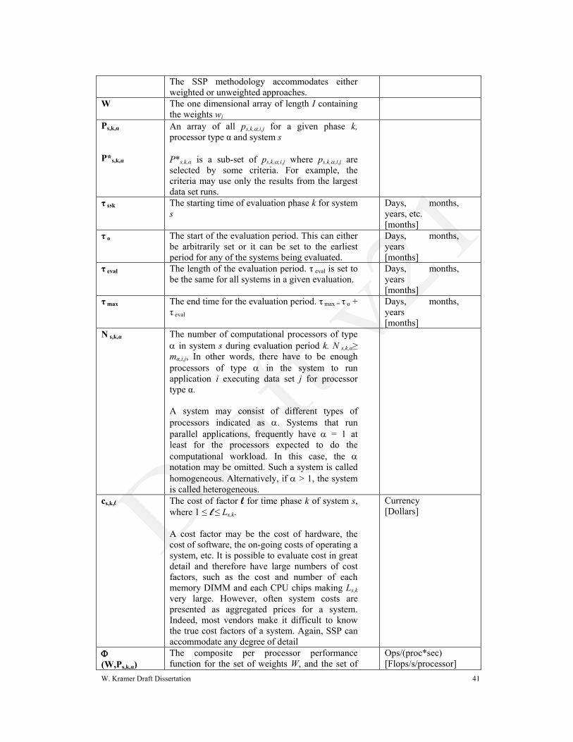
The SSP methodology accommodates either
weighted or unweighted approaches.
W The one dimensional array of length I containing
the weights wi
Ps,k,α
P*s,k,α
An array of all ps,k,,i,j for a given phase k,
processor type α and system s
P*s,k,α is a sub-set of ps,k,,i,j where ps,k,,i,j are
selected by some criteria. For example, the
criteria may use only the results from the largest
data set runs.
τ s,k The starting time of evaluation phase k for system
s
Days, months,
years, etc.
[months]
τ o The start of the evaluation period. This can either
be arbitrarily set or it can be set to the earliest
period for any of the systems being evaluated.
Days, months,
years
[months]
τ eval The length of the evaluation period. τ eval is set to
be the same for all systems in a given evaluation.
Days, months,
years
[months]
τ max The end time for the evaluation period. τ max = τ o +
τ eval
Days, months,
years
[months]
N s,k,α The number of computational processors of type
in system s during evaluation period k. N s,k,α≥
mα,i,j, In other words, there have to be enough
processors of type in the system to run
application i executing data set j for processor
type α.
A system may consist of different types of
processors indicated as . Systems that run
parallel applications, frequently have = 1 at
least for the processors expected to do the
computational workload. In this case, the
notation may be omitted. Such a system is called
homogeneous. Alternatively, if > 1, the system
is called heterogeneous.
cs,k,l The cost of factor l for time phase k of system s,
where 1 ≤ l ≤ Ls,k.
A cost factor may be the cost of hardware, the
cost of software, the on-going costs of operating a
system, etc. It is possible to evaluate cost in great
detail and therefore have large numbers of cost
factors, such as the cost and number of each
memory DIMM and each CPU chips making Ls,k
very large. However, often system costs are
presented as aggregated prices for a system.
Indeed, most vendors make it difficult to know
the true cost factors of a system. Again, SSP can
accommodate any degree of detail
Currency
[Dollars]
(W,Ps,k,α)
The composite per processor performance
function for the set of weights W, and the set of
Ops/(proc*sec)
[Flops/s/processor]

W. Kramer Draft Dissertation 42
per processor performance P for performance
phase k for processor type α on system s. This
will be discussed in detail later.
SSPs,k Sustained System Performance for system s for
phase k.
Equation 3-3: Sustained System Performance for
system s during phase k
A
ksks
ks
NPWSSP ks
,
1, ,,,,,
Operations/time
[Flops/sec]
Potencys The potential of a system s to produce useful
work results over a period of time. Potency was
chosen for this term since it means “capacity to
be, become, or develop;”18
Equation 3-4: A system‟s potency is a reflection of its
ability to do productive work.
sPotency
k1
sK
s,kSSP s,k1
min( ,max )
s,kmin( ,
max ) ; s,k max
There will be more discussion of systems with
phases in Chapter 4.
Operations
[Flops]
Note: it is possible
to consider Potency
as a rate
[Flops/sec]
multiplied by a
time period [day,
months, years…].
Hence Potency is
can also be
expressed more as
integrated
performance over
time.
[e.g.
TFlops/sec*Years
or
GFlops/sec*Month
s]
Costs The cost of system s. Cost is composed of
different components cs,k,l.
Equation 3-5: Costs are used for setting value of a solution
sCost cs,k,ll1
s,kL
k1
sK
Currency
[Dollars]
Values The ratio of potency to cost for system s
Equation 3-6: Value of a solution is its potency relative
to its cost
Operations/Currenc
y
[Flops/$]

W. Kramer Draft Dissertation 43
Cost
PotencyValue
s
s
s
Potency and Cost are influenced by the number of
processors, Ns,k,, but the degree of influence
cannot be assumed to be equivalent for many
reasons including economies of scale and
business strategies. Table 3-3: Formula‟s for determining the SSP.
3.8 Running Example Part 1 – Applications
Our running example has 3 benchmarks; A, B, and C, each with one problem set.
Hence I = 3. Each benchmark uses only MPI so there is a mapping of one MPI task to
one CPU. Since each benchmark has only one data set, J = 1, it is omitted for clarity.
Three systems are evaluated, each with uniform processors, so S = 3. = 1 and is
omitted for clarity.
Table 3-4 below summarizes the benchmarks‟ characteristics. The operation
counts can be determined in a variety of ways, but most systems today have a utility
to either count the number of operations for a problem run.
Application Total
Operation
Count, f
GFlops
Concurrency,
m
Processors
Work done in
each task, a.
GFlops/processor
A 549,291 384 1430
B 310,842 256 1214
C 3,143,019 2,048 1535
Table 3-4: This table shows the basic performance characteristics for the three benchmarks in our example

W. Kramer Draft Dissertation 44
Before examining the proposals for the systems, it is possible to assume these
benchmarks were run on a baseline system, such as NERSC‟s Power 3 system
Seaborg. Table 3-5 shows the per processor performance of these runs.
Application Wall Clock Runtime,
t
Seconds
Per Processor
Performance, p
Gflops/sec/processor
A 42,167 0.034
B 9,572 0.127
C 12,697 0.121
Table 3-5: Baseline performance of benchmarks on an existing system.
3.9 Aligning the Timing of the Phases
Evaluations should have the same period of performance for all systems. Since
systems have different timings for availability or delivery, aligning these periods is
necessary for a fair comparison.
Additionally, for each system, there can be more than one phase of system
evolution. A phase is characterized by the system having different components and/or
additional components that make the potency different than the previous phase. The
cost of each phase, as well as the potency maybe different as well. For the evaluation
there is a period set, τeval to limit the length of the evaluation period. τeval is often
related to how long the technology is to be used. NERSC uses 36 months and DOD-
HPC Modernization program uses four years19
.

W. Kramer Draft Dissertation 45
Systems are unlikely to be delivered at exactly the same time and it is not
equitable to use the individual system delivery times as the starting point since the
price/performance ratio of a system delivered later is almost certainly less than one
delivered earlier – all other things being equal. However, another consequence of
later delivery is lost computing opportunities. A simple thought experiment shows
why this is important. Suppose an organization has two choices: have a 100 teraflop/s
system deployed in January 1, 2007 or a 500 teraflop/s system deployed in January 2,
2012. Assume they have the same real cost and assume sustained performance of the
2012 system is also five times that of the 2007 system. A valid question could be
along the lines of “How long is it before the organization has the same potency as it
will in April 1, 2013?” The answer is it takes 1.25 years of use of the 2012 system to
provide the same potency as the 2007 system. The impact of choosing to wait for the
system with the better price/performance ratio is the organization has no computing
for 5 years at all, and then takes 1.25 years to make up the lost computing power.
So, are the two systems equal in value to the organization? It depends on the
organizational goals and many factors such as whether the same number of people
can gain the same insight in 25% of the wall clock time and whether there are
opportunities lost by having no computing for 5 years. What is clear is, the phase
boundaries have to be adjusted for each system in the evaluation in order to fairly
represent the value of different solutions. The adjustments that have to be made are
straightforward. Algorithms for the adjustments are shown in the Table 3-3:
Formula‟s for determining the SSP.

W. Kramer Draft Dissertation 46
First, the system with the earliest delivery date is identified, which sets the
starting point, τ o to be beginning of the evaluation period. It may be that the
organization needs a system by a certain time, so the evaluation period has to start no
later than a given deadline. In this case, τ o can set to the earliest of the First System
Arrival/”No Later Than” deployment time set by the evaluators – whichever is
earliest.
Not only can different systems arrive for use at different times, it may be that the
best overall solution is to have systems evolve through time, based on optimizing
different price points. A way of describing the timing of each phase a system goes
through, which is τ s,k is needed. For each system s, there will be one or more stages,
indicated by k.
Because solutions cannot wait indefinitely for the ending time τ max, the evaluation
must be set by the evaluators, and is specified as τ max = τ o + τ eval. Once τ o and τ max
are determined, all the systems solutions being evaluated need to be adjusted to that
interval. This is done by adjusting the starting period of all the systems to τ o, and
assigning the performance and cost for a system during this period to be 0. Likewise,
for the systems whose delivery would take them past τ max, no performance or cost is
counted for that system.
Figure 3-1and Figure 3-2show the impact of these adjustments. Figure 3-1 shows
two systems being evaluated. System 1 arrives and is deployable before System 2 and
has a single phase. System 2 arrives and is deployed after System 1 and has an
improvement part way through the evaluation process, triggering the second phase.

W. Kramer Draft Dissertation 47
τeval
Figure 3-1: The proposed deployment time and SSP of two systems.
Assuming System 1 is deployed before any time limitation such as τ NLT, the
deployment of System 1 defines τ o for both systems. Since System 2 arrives after τ o,
the performance and cost for System 2 is set to 0 until it arrives. The end of the
evaluation period is also set based on System 1 arrival/deployment time. After these
adjustments are used the evaluation periods are shown in Figure 3-2.
SSP
τ 0 = τ1,1 Ti
m
e
τ
2
,
1
τ2,2 τmax
max

W. Kramer Draft Dissertation 48
τeval
Figure 3-2: SSP performance chart after periods are aligned. For clarity τ́2,k replaces τ2,k
3.10 Running Example Part 2 – Systems
Our running example assumes three different systems are being evaluated. System
1 has a high per processor performance, but each processor is relatively expensive.
Because it is under development, it can only be delivered 9 months after System 2.
System 2 is a system that is currently available for immediate delivery and consists of
processors that are modest in performance, but are also relatively inexpensive.
System 3 is a system that has per processor performance that is close to System 2.
While part of the system can be delivered immediately, ¾ of the system is delayed by
4 months due to manufacturing backlog. Furthermore, the first ¼ of System 3 will
perform 20% slower until the rest of system is delivered. System 3‟s per processor
cost is lower than either System 1 or System 2.
SSP
Ti
m
e
τ́ 2,2 τ́2,3 τmax
max
τ ́ 2,1 = τ 0 =
τ1,1

W. Kramer Draft Dissertation 49
For simplicity, assume other aspects of the systems are identical except for the
cost. Note the “cost” can be any calculation – from only initial hardware cost to
complete total cost of ownership. The costs in the example approximate 6 years Total
Cost of Ownership for this scale system.
Table 3-6 indicates the system parameters for the running example. The time
period of the evaluation is set at 36 months – a typical time period during which large
systems have the most impact.
System Delivery
Delay
Months
Number of
Compute
Processors
Cost
Dollars
System 1 9 9,000 $59,000,000
System 2 0 10,000 $68,000,000
System 3
- Phase 1
- Phase 2
0
6
3,500
14,000
$57,000,000
Table 3-6: Specifications of solutions being considered
From this information one cannot determine the solution that is the best value.
The benchmark runtimes for the three systems is shown in Table 3-7, and the
resulting per processor performance in Table 3-8.
Runtimes in seconds of
Benchmarks on each
System
A B C

W. Kramer Draft Dissertation 50
System 1 3810 1795 2303
System 2 3598 2010 3170
System 3
- Phase 1
- Phase 2
4930
4103
2622
2185
2869
2391
Table 3-7: Benchmark Runtimes in Seconds for Three Systems
Per Processor Performance in
GFlops/s of Benchmarks on
each System
A B C
System 1 .375 .676 .666
System 2 .398 .604 .484
System 3
- Phase 1
- Phase 2
.290
.348
.463
.556
.535
.642
Table 3-8: Per processor performance of three benchmarks
3.11 The Composite Performance Function (W,P)
The composite performance function can be chosen in different ways. There are
many possible functions, depending on the data and goals. Several may be
appropriate for a given evaluation. Which functions are appropriate for different

W. Kramer Draft Dissertation 51
performance measures is an on-going discussion and is covered in [Bucher and
Martin87]20
, [Flemming and Wallace86]21
, [Smith88]22
, [Lilja2000]23
, [Hennessey
and Patterson]24
, [John and Eeckhout]25
, [Helin and Kaski]26
, and [Mashey2004]27
.
The SSP method can use any appropriate composite. Hence, this section does not try
to do an exhaustive study of all possible functions, but rather is a general discussion
of several likely functions and how to implement them.
Recall wi and Ps,k, as defined above. Some of the more typical composite
functions are Arithmetic Mean, Harmonic Mean and Geometric Mean – all of which
can use either weighted or unweighted data. More advanced statistical functions could
be used such as the t test or an Analysis of Variance28
.
Equation 3-7, Equation 3-8, and Equation 3-9 show the implementation of the
three more common means. If wi = 1 for all i, then the means are unweighted.
Equation 3-7: Weighted Arithmetic Mean
Equation 3-8: Weighted Harmonic Mean
I
i
i
I
i jji
i
wAM
w
Jw
i
p
1
1 1,
I
i jji
i
I
i
J
j
i
wHM J w
w
i
i
p1 1,
1 1

W. Kramer Draft Dissertation 52
Equation 3-9: Weighted Geometric Mean
3.12 The Only Real Metric – How Long Does a System Take to
Solve a Problem
The number of operations a computer uses to solve a given problem varies
dramatically based on the computer architecture, its implementation, and the
algorithm used to solve the problem. While this has been the case from the dawn of
computing, the problem of deciphering how much work is done by different systems
has gotten harder with time. Early performance results on distributed memory
computers were so notorious for providing misleading information that it prompted
Dr. David Bailey to publish his Twelve Ways to Fool the Masses When Giving
Performance Results on Parallel Computers29
paper in 1994. In this paper, 7 of the 12
ways (ways 2, 3, 4, 6, 8, 9, and 10) relate to using measurements that are misleading
for comparisons that vary depending on the computer system being used or doing a
subset of the problem. New processors and increasing scale compound this problem
by causing more and more basic computer operations to be done for a given amount
of usable work. Different algorithms, programming languages and compilers all
influence performance in addition to the computer architecture and implementation.30
Many performance evaluators recognize that Time To Solution is the best –
maybe only – meaningful measure of the potential a computer provides to address a
problem. If the system is to be used for a single application, assessing time to solution
I
i
J i
j
wiji
w
p
I
i
J i
j i
wGM
1 1,
1 1
1

W. Kramer Draft Dissertation 53
is relatively straight forward. One takes an application, tests the systems with one or
more problem sets and compares the time it takes for the application to solve the
problem. An example of this approach is a metric commonly used by the climate
modeling community which is the number of simulated years per unit of wall clock
time. Weather forecasting has similar metrics – the wall clock time it takes to produce
a given forecast. Chemical and materials simulations could have a similar measure –
the time it takes to simulate a compound with a fixed number of atoms, for example.
In these cases, as long as the algorithm and problem (the same resolution, the same
precision of modeling physical processes, etc.) remains unchanged, there is a fair
comparison based on time to solutions.
A more challenging, but more commonly occurring situation is when computer
systems are evaluated for use with different applications and/or domains because
there is no common unit of work that can be used for comparison. That is, it is not
meaningful, for example to compare the number of years a climate simulation
produces in a given wall clock time to the size of a protein that is folded in a chemical
application. Similarly, if the problems or physics the algorithms represent change
within an application area, the comparison of the amount work done is not clear cut.
Finally, if the implementation of an application has to fundamentally change for a
computer architecture the number of operations may dramatically different.
It is common, therefore, for performance evaluators to use the number of
instructions executed per second (also known as operations per second) or other less

W. Kramer Draft Dissertation 54
meaningful measures methods (e.g. peak performance, Top-500 lists, etc.), This
approach leads to easily misunderstanding comparative results.
SSP solves this problem since the operation count used in the calculation of SSP
is fixed once for the benchmark test and is based on the problem solution executing
on a reference (presumably efficient) system. If the problem is also fixed, the only
invariant is the time the test takes to run to solution on each system.
3.12.1 Comparison Based on Time to Solution
To show SSP is a measure of time to solution if the operation count is based on a
reference count, consider the following. For each combination of an application and
problem set, i,j, the number of operations fi,j is fixed as is the concurrency, mi,j. As
shown above,
jisji
ji
jisji
ji
jistm
f
tm
fp
,,,
,
,,,
,
,,
1*
*
Equation 3-10: The per processor performance for a test depends on the time to complete that test
For simplicity, but without loss of generality, assume an unweighted composite
function. Again for simplicity, use the standard mean and assume all the processors in
a system are homogeneous and there is a single phase. The per processor performance
can be expressed as

W. Kramer Draft Dissertation 55
I
t
I
m
f
I
tm
f
P
I
i
J
j ji
I
i
J
j ji
jiI
i
J
j jiji
ji
s
1 1 ,1 1 ,
,
1 1 ,,
,)
1(
*
)()1
*(
Equation 3-11: Per processor performance for a system depends on time to solution
The equation of SSP performance between two system, s and s’ with the same
number of computer processors, N, can be expressed as follows:
jis
jis
jis
jis
ji
ji
ji
ji
jisji
ji
jisji
ji
s
s
t
tN
It
It
Im
f
Im
f
Itm
fN
Itm
fN
SSP
SSP
,,'
,,'
,,'
,,
,
,
,
,
,,',
,
,,,
,
'
*
)1
(
)1
(
*
(
(
)1
**
)1
**
Equation 3-12: Comparing SSP values is equivalent to comparing time to solution
Hence, SSP compares the sum of the time to solution for the tests. From this, it
is clear that if the number of processors is different for the two systems, then the SSP
is a function of the times to solution and the number of processors. It the systems
have multiple phases, the SSP comparison is dependent on the time to solutions for
the test, the number of processors for each phase and the start time and duration for
each phase. This can be further extended for heterogeneous processors and/or for
different composite functions without perturbing the important underlying fact the
SSP compares time to solution.
3.13 Attributes of Good Metrics
There are benefits of using different composite methods, based on the data. The
approach of using the harmonic mean was outlined in a 1982 Los Alamos technical

W. Kramer Draft Dissertation 56
report31
[Bucher and Martin1982]. It should be noted that at the time, the workload
under study was a classified workload with a limited number of applications. In fact,
the authors dealt with “five large codes”. The paper outlines the following process.
1. Workload Characterization: Conduct a workload characterization study using
accounting records to understand the type and distribution of jobs run on your
systems.
2. Representative Subset: Select a subset of programs in the total workload that
represent classes of applications fairly and understand their characteristics.
This included the CPU time used, the amount of vectorization, the rate of
Floating Point Operation execution and I/O requirements.
3. Weighing the influence of the Applications: Assign weights according to
usage of CPU time of those programs on the system.
4. Application Kernels: Designate portions (kernels) of the selected programs to
represent them. These kernels should represent key critical areas of the
applications that dominate the runtime of the applications.
5. Collect Timing: Time the kernels on the system under test using wall clock
time.
6. Compute a Metric: Compute the weighted harmonic mean of kernel execution
rates to normalize the theoretical performance of the system to a performance
that would likely be delivered in practice on the computing center‟s mix of
applications.

W. Kramer Draft Dissertation 57
Bucher and Martin were focused on the evaluation of single processors – which
was the norm at the time. As stated, the implementation of this methodology suffers
from some pragmatic problems:
1. It is difficult to collect an accurate workload characterization given that many
tools for collecting such information can affect code performance and even
the names of the codes can provide little insight into their function or
construction (the most popular code, for instance, is „a.out‟).
2. Most HPC Centers support a broad spectrum of users and applications. The
resulting workload is too diverse to be represented by a small subset of
simplified kernels. For example, at NERSC, there are on the order of 500
different applications used by the 300-350 projects every year.
3. The complexity of many supercomputing codes has increased dramatically
over the years. The result is that extracting a kernel is an enormous software
engineering effort and maybe enormously difficult. Furthermore, most HPC
codes are made up of combinations of fundamental algorithms rather than a
single algorithm.
4. The weighted harmonic mean of execution presumes the applications are
either serial (as was the case when the report was first written) or they are run
in parallel at same level of concurrency. However, applications are typically
executed at different scales on the system and the scale is primarily governed
by the science requirements of the code and the problem data set.
5. This metric does not take into account other issues that play an equally
important role in decisions such as the effectiveness of the system resource

W. Kramer Draft Dissertation 58
management, consistency of service, or the reliability/fault-tolerance of the
system. The metric also is not accurate in judging heterogeneous processing
power within the same system – something that may be very important in the
future.
John and Eeckhout32
indicate the overall computational rate of a system can be
represented as the arithmetic mean of the computational rates of individual
benchmarks if the benchmarks do not have an equal number of operations.
Nevertheless, there are attributes of making a good choice of a composite function.
Combining the criteria from [Smith1988]33
and [Lilja2000]34
provides the following
list of good attributes.
Proportionality – a linear relationship between the metric used to estimate
performance and the actual performance. In other words, if the metric
increases by 20%, then the real performance of the system should be expected
to increase by a similar proportion.
o A scalar performance measure for a set of benchmarks expressed in
units of time should be directly proportional to the total time
consumed by the benchmarks.
o A scalar performance measure for a set of benchmarks expressed as a
rate should be inversely proportional to the total time consumed by the
benchmarks.
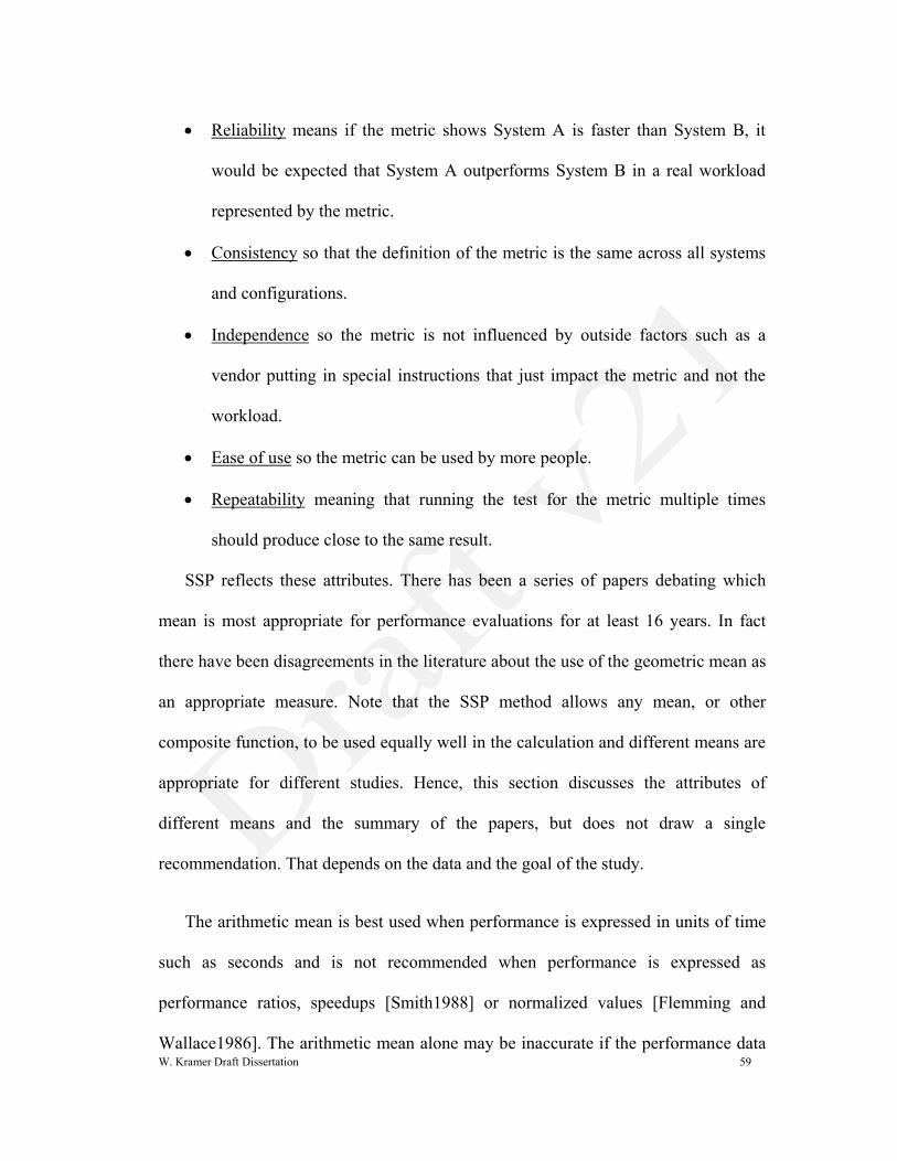
W. Kramer Draft Dissertation 59
Reliability means if the metric shows System A is faster than System B, it
would be expected that System A outperforms System B in a real workload
represented by the metric.
Consistency so that the definition of the metric is the same across all systems
and configurations.
Independence so the metric is not influenced by outside factors such as a
vendor putting in special instructions that just impact the metric and not the
workload.
Ease of use so the metric can be used by more people.
Repeatability meaning that running the test for the metric multiple times
should produce close to the same result.
SSP reflects these attributes. There has been a series of papers debating which
mean is most appropriate for performance evaluations for at least 16 years. In fact
there have been disagreements in the literature about the use of the geometric mean as
an appropriate measure. Note that the SSP method allows any mean, or other
composite function, to be used equally well in the calculation and different means are
appropriate for different studies. Hence, this section discusses the attributes of
different means and the summary of the papers, but does not draw a single
recommendation. That depends on the data and the goal of the study.
The arithmetic mean is best used when performance is expressed in units of time
such as seconds and is not recommended when performance is expressed as
performance ratios, speedups [Smith1988] or normalized values [Flemming and
Wallace1986]. The arithmetic mean alone may be inaccurate if the performance data

W. Kramer Draft Dissertation 60
has one or more values that are far from the mean (outlier). In that case, the arithmetic
mean together with the standard deviation or a confidence interval is necessary to
accurately represent the best metric. [John2004]35
concludes the weighted arithmetic
mean is appropriate for comparing execution time expressed as speedups for
individual benchmarks, with the weights being the execution times.
The harmonic mean is less susceptible to large outliers and is appropriate when
the performance data is represented as rates. The unweighted harmonic mean for a
system phase can be expressed as total operation count for all benchmarks divided by
the total time of all benchmarks as shown in Equation 3-8.
Use of geometric means as a metric is not quite as settled. [Smith1988] says it
should never be used a metric, while [Flemming and Wallace1986] indicates it is the
appropriate mean for normalized numbers regardless of how they were normalized.
They also note it addresses the issue of data that has a small number of large outliers.
This paper also points out the geometric means can be used for numbers that are not
normalized initially, but when the resulting means are then normalized to draw
further insight.
[Mashey2004] examines the dispute and identifies that there are reasons to use all
three means in different circumstances. Much of the previous work assumed some
type of random sampling from the workload in selecting the benchmarks. This paper
notes that geometric means have been used in many common benchmark suites such
as the Livermore FORTRAN Kernels36
and the Digital Review CPU 237
benchmarks.
This paper organizes benchmark studies into three categories, and each has its

W. Kramer Draft Dissertation 61
appropriate methods and metrics. The first and most formal category is WCA
(Workload Characterization Analysis), which is a statistical study of all the
applications in a workload, including their frequency of invocation and their
performance. WCA is equivalent to the methodology outlined in Bucher and Martin.
This type of analysis provides a statistically valid random sampling of the workload.
Of course, WCA takes a lot of effort and is rarely done for complex workloads. WCA
also cannot be done with standard benchmark suites such as NPB or SPEC. While
such suites may be related to a particular workload, by their definition, they cannot be
random samples of a workload.
The Workload Analysis with Weights (WAW) is possible after extensive WCA
because it requires knowledge of the workload population. It can predict workload
behavior under varying circumstances.
The other type of analysis in [Mashey2004] is the SERPOP (Sample Estimation
of Relative Performance of Programs) method. In this category, a sample of a
workload is selected to represent a workload. However, the sample is not random and
cannot be considered a statistical sample. SERPOP methods occur frequently in
performance analysis, and many common benchmark suites including SPEC, NPB as
well as many acquisition test suites fit this classification. In SERPOP analysis, the
workload should be related to SERPOP tests, but SERPOP does not indicate at all the
frequency of usage or other characteristics of the workload.
The impact of the assumptions in early papers (fixed time periods, random
samples, etc.) that discuss the types of means are not valid for SERPOP analysis.

W. Kramer Draft Dissertation 62
Because of this, the geometric mean has several attributes that are appropriate for
SERPOP analysis. In particular, [Mashey2004] concludes geometric means are
appropriate to use for ratios since taking ratios converts unknown runtime
distributions to log-normal distributions. Furthermore, geometric means are the
appropriate mean for SERPOP analysis without ratios when there are many reasons
the distribution of a workload population is better modeled by a log-normal
distribution.
3.13.1 Running Example Part 3 – Holistic Analysis
For our running example, the arithmetic mean will be used to calculate the SSP
and Solution Potential.
System
Evaluation
using SSP
Average Per
Processor
Performance
GFlops/s
System SSP
using the
mean of the
three
benchmarks
GFlops/sec *
Months
Solution
Potential
GFlops/s *
Months
Solution
Value
GFlops/s-
Months/
Million $
System 1 .573 5,155 139,180 2,359
System 2 .495 4,953 178,294 2,622
System 3 225,426 3,955

W. Kramer Draft Dissertation 63
- Phase 1
- Phase 2
.429
.515
1,503
7,214
9,017
216,426
Table 3-9: Per processor performance of three benchmarks
While System 1 has the highest per processor performance, because it is delivered
quite a bit later than the other systems, it has the lowest potential and value. System 2,
even though it is delivered at full scale earliest, has the middle value. System 3, with
two phases clearly has the highest value for the evaluation using these benchmarks.
3.14 Chapter Conclusion
The SSP method is flexible and comprehensive, yet is an easy concept to
understand. It uses the most meaningful measure for computer users to make its
comparisons – time to solution. The method works with any set of performance tests
and for both homogeneous and heterogeneous systems. The benchmarks can have as
many data sets as needed and be scaled to the desired degree of precision and effort.
W. Kramer Draft Dissertation 64
Chapter 4: Practical Use of Sustained System
Performance for HPC Systems - How SPP
works in Evaluation and Selection
4.1 Chapter Summary
This chapter provides a number of examples using the SSP method to evaluate
and vet large systems. It traces the evolution of the SSP method over a 10 year effort
as it became more sophisticated and effective. Large HPC systems are complex and
evaluated/purchased only once every three to five years. Hence 10 years gave the
opportunity to have and assess four generations of SSP. As part of the observations of
SSP, it can be seen that the SSP method gives both the purchaser and the supplier of
systems protection. The supplier has freedom to adjust the schedule of deliverables
and the purchaser is protected by a guarantee of a fixed amount of performance
delivered in a certain time period. The degree of adjustments can be constrained as
well, so it is possible to arrange incentives for early delivery or delivery of more
effective systems.
4.2 Review of Chapter 3
Chapter 3 discusses the SSP method for overall performance assessment that is
one method to evaluate the Performance of a system. While SSP is not the only
measure used to assess a system‟s potential to solve a set of problems, it is one of the
few that, if properly constructed, can be used for all four purposes of benchmarks.
Section 3.8 discussed a simplified example of a problem. This chapter takes the SSP
approach from the previous chapter and examines the use of SSP in different real
world evaluations and selection issues in a variety of circumstances.

W. Kramer Draft Dissertation 65
4.3 A Real World Problem, Once Removed
It is not possible to disclose the details of actual procurement submissions or
evaluations since the information is provided by vendors to the requesting
organization for evaluation and selection and is considered proprietary. However, it is
possible to craft a summary that is based on real world information from such a
procurement that is sufficient to properly illustrate the use of SSP.
Imagine an organization evaluating large scale systems for a science or
engineering workload. The organization determines functional and performance
requirements and creates a benchmark suite of applications and other tests. It then
solicits and receives information from potential vendors as to how well their
technology meets the requirements and performs according to the benchmarks. In
many cases the response is a combination of actual measurements and projections.
For simplicity, assume the only distinguishing characteristics under evaluation are the
specified benchmark performance on a per processor basis shown in Table 4-1. They
are the set of p,s,k,,i,j that was defined in Table 3-2: SSP Definitions
There are five proposed systems (S= 5). Five application benchmarks are used to
calculate the SSP, so I = 5. While the applications run at medium to high
concurrency, they operate at different concurrencies. Each application has been
profiled on a reference system so its operation count is known for particular problem
sets. In this case, each application has one problem, so Ji = 1 for this discussion.
Further, assume these systems are composed of homogeneous processors so α= 1, so
it, too, is set to 1.

W. Kramer Draft Dissertation 66
As defined in Table 3-3, in order to calculate the per processor rate of the
applications, ps,k,1,i,1, the total operation count of the benchmark is divided by the
concurrency of the benchmark to give the average per processor operation count and
then divided again by the wall-clock runtime of the benchmark. Four of the five
systems proposed had phased technology introduction, with each of these having
Ks=2.
The cost data includes basic hardware and software system costs and the
operating and maintenance costs for three years from the delivery of the earliest
system. In order to protect the proprietary information provided by vendors, the cost
data is expressed relative to the lowest cost proposed. Delivery times all are relative
to the earliest system delivery and set to the number of months after the system with
the earliest delivery time

W. Kramer Draft Dissertation 67
System 1 System 2 System 3 System 4 System 5
Phase 1
Application Benchmark 1 GFlops/sec per Processor 0.31 0.20 0.74 N/A 0.22
Application Benchmark 2 GFlops/sec per Processor 0.40 0.30 1.31 N/A 0.06
Application Benchmark 3 GFlops/sec per Processor 1.35 0.17 0.64 N/A 1.19
Application Benchmark 4 GFlops/sec per Processor 1.00 2.34 5.99 N/A 1.12
Application Benchmark 5 GFlops/sec per Processor 0.49 0.51 1.02 N/A 0.45
Delivery Months after earliest delivery 3 0 6 N/A 0
Number of Processors 768 512 512 N/A 512
Phase 2
Application Benchmark 1 GFlops/sec per Processor 0.31 0.19 0.74 0.10 0.22
Application Benchmark 2 GFlops/sec per Processor 0.40 0.34 1.31 0.30 0.06
Application Benchmark 3 GFlops/sec per Processor 1.35 0.16 0.64 0.39 1.19
Application Benchmark 4 GFlops/sec per Processor 1.00 1.54 5.99 0.92 1.12
Application Benchmark 5 GFlops/sec per Processor 0.49 0.26 1.02 0.14 0.45
Delivery Months after earliest delivery 12 22 18 3 6
Number of Processors 1536 1024 1408 5120 2048
Cost Factor Relative cost among proposals 1.65 1.27 1.27 1.16 1.00
Table 4-1: Per processor performance, p, for each system, phase and benchmark for a hypothetical system purchase. These responses are anonymized and adjusted from actual vendor responses for major procurements. Systems 1, 2, 3, and 5 are proposed to be delivered in two phases. System 4 is a single
delivery. The per-processor performance of five application benchmarks is shown. The systems would be delivered at different times. The table shows the delivery date relative to the earliest system.

W. Kramer Draft Dissertation 68
Figure 4-1: System parameters for Phases 1. Note System 4 is a single phase and it shown in the Phase 2 chart.
Figure 4-2: System parameters for Phases 2.
Figure 4-1 and Figure 4-2 show the same data as in Table 4-1, but in graphical
form. The challenge of an organization is to use this data to decide which system is
the best value for the organization‟s mission and workload. As can be seen in Figure
4-1and Figure 4-2, the answer of which option provides the system with the best
0
100
200
300
400
500
600
700
800
900
0.00
1.00
2.00
3.00
4.00
5.00
6.00
System 1 System 2 System 3 System 4 System 5
Nu
mb
er
of
CP
Us
GF
op
s/s
ec p
er
pro
cesso
r
Systems
Phase 1 Performance
ABM 1
ABM 2
ABM 3
ABM 4
ABM 5
Number of CPUs
0
1000
2000
3000
4000
5000
6000
0.00
1.00
2.00
3.00
4.00
5.00
6.00
System 1 System 2 System 3 System 4 System 5
Nu
mb
er
of
CP
Us
GF
lop
s/s
ec p
er
pro
cesso
r
Systems
Phase 2 Performance
ABM 1
ABM 2
ABM 3
ABM 4
ABM 5
Number of CPUs
W. Kramer Draft Dissertation 69
value is not obvious from the benchmark performance alone. Without understanding
the number of CPUs in different systems, the timing of different phases and the cost
of the different systems, an evaluation runs the risk of not picking best value system.
4.4 Different Composite Functions
As discussed in Chapter 3, different composite functions can be used for SSP
calculations – including all three means. The best composite function to use depends
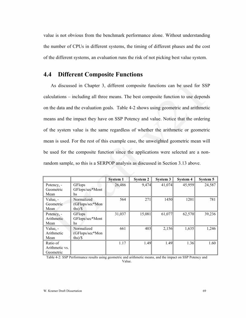
on the data and the evaluation goals. Table 4-2 shows using geometric and arithmetic
means and the impact they have on SSP Potency and value. Notice that the ordering
of the system value is the same regardless of whether the arithmetic or geometric
mean is used. For the rest of this example case, the unweighted geometric mean will
be used for the composite function since the applications were selected are a non-
random sample, so this is a SERPOP analysis as discussed in Section 3.13 above.
System 1 System 2 System 3 System 4 System 5
Potencys -
Geometric
Mean
GFlops
GFlops/sec*Mont
hs
26,486 9,474 41,074 45,959 24,587
Values -
Geometric
Mean
Normalized
(GFlops/sec*Mon
ths)/$
564 271 1450 1201 781
Potencys -
Arithmetic
Mean
GFlops
GFlops/sec*Mont
hs
31,037 15,081 61,077 62,570 39,236
Values -
Arithmetic
Mean
Normalized
(GFlops/sec*Mon
ths)/$
661 403 2,156 1,635 1,246
Ratio of
Arithmetic vs.
Geometric
1.17 1.49 1.49 1.36 1.60
Table 4-2: SSP Performance results using geometric and arithmetic means, and the impact on SSP Potency and Value.

W. Kramer Draft Dissertation 70
4.5 Impact of Different Means
The relationship of means is HM ≤ GM ≤ AM38
. Comparing the results of
arithmetic mean and geometric mean show there are differences in the expected
performance of the system. Note the ratio of performance between systems is not
equal between means but in every case, the geometric mean is lower than the
arithmetic. Furthermore, using the arithmetic mean, the order of best to worst price
performance is Systems 3, 4, 5, 1 and 2. Using the geometric mean, the order is 3, 4,
5, 1 and 2. So the ordering of the system is preserved regardless of the mean used in
this situation. In another example, running the SSP-4 test suite (discussed in detail
later in this chapter) on different technology systems at Lawrence Berkeley National
Laboratory (LBNL) (systems named Seaborg, Bassi and Jacquard) and Lawrence
Livermore National Laboratory (LLNL) (system name Thunder) using the arithmetic,
harmonic and geometric means changes the absolute value of the SSP, but does not
change the order of performance estimates.
Seaborg
(LBNL)
Bassi
(LBNL)
Jacquard
(LBNL)
Thunder
Cluster
(LLNL)
Computational
Processors
6224 888 4096 640
Arithmetic
SSP-4
1,445 1,374 689 2,270
Geometric
SSP-4
902 835 471 1,637
Harmonic
SSP-4
579 570 318 1,183
Table 4-3: Another example of using different means that do not change the ordering of system performance

W. Kramer Draft Dissertation 71
Since the ordering of the means is consistent, and the harmonic mean is less
appropriate as a composite function for benchmarks that change their concurrency,
the arithmetic or geometric means are used at NERSC and their affects are discussed
in Sections 3.11 and 4.4. For the examples in Section 3.2, the arithmetic mean is used.
4.6 System Potency
Delivery of each system as in our example would occur at different times.
Graphing the monthly values of the SSP for each system over time as shown in
Figure 4-3 differentiates some of the systems. For example, System 2, despite having
good per processor performance, had a low Potency since it has relatively few CPUs.
To be the best value it would have to be 5 or 6 times less expensive than other
alternatives. At the end of the evaluation period, System 3 provided the best sustained
performance, followed by system 4. Yet, System 3 was upgraded after System 2 and
5, and System 4 had only a single phase so it is not clear from this graph which
system has the most potency, let alone the best value.
Figure 4-3: A graph of the example SSP value over time for the five systems. This is using the geometric mean as the composite function.
Anonymized SSP Evaluation
0
500
1000
1500
2000
2500
3000
1 3 5 7 9 11 13 15 17 19 21 23 25 27 29 31 33 35
Month from initial system
SS
P G
Flo
p/s
System 1
System 2
System 3
System 4
System 5

W. Kramer Draft Dissertation 72
As a thought experiment, think about the situation where there are two systems,
and System 1 is twice as fast as System 2. In other words, it has an SSP1,k = 2 *
SSP2,k. Assume further, System 1 is also twice as expensive System 2. The first thing
to recall is having twice the SSPs,k, does not mean the system has twice the Potency.
In order to have twice the Potency, the two systems have to be available at the exact
same time. This may be case with a commodity such as at a local computer store but
is highly unlikely for HPC systems. Nonetheless, if the two systems arrived at
identical times, and the Potency of System 1 was twice that of System 2, and the cost
of System 1 was twice that System 2, they would have the same value with regard to
the SSP. Further, in most major system evaluations, there are multiple cost functions
evaluated – for example the Initial System Cost and the Total Cost of Ownership.
Having all the cost functions identical is also unlikely.
But even if the Value of the two systems is exactly identical, that only reflects the
performance component based on the selected benchmark tests. The overall value of
the systems will almost certainly be different if the other aspects of PERCU are added
to the evaluation. Or evaluators may choose to add second order benchmark tests,
possibly to reflect use cases that are less important but to increase the accuracy of the
SSP for the real workload as the “tie breaker”.
4.7 Using Time to Solution in SSP
The way to calculate an SSP value using time to solution for the tests is
straightforward and illustrated below.

W. Kramer Draft Dissertation 73
Tests (a)
Tasks
(b)
Reference
GFlop
Count
(c)
Measured Wall
Clock Time to
Solution (Sec) for
the Evaluated
System
(d)
Processing
rate per
core
(GFlops/s)
CAM 240 57,669 408 0.589
GAMESS 1024 1,655,871 2811 0.575
GTC 2048 3,639,479 1492 1.190
IMPACT-T 1024 416,200 652 0.623
MAESTRO 2048 1,122,394 2570 0.213
MILC 8192 7,337,756 1269 0.706
PARATEC 1024 1,206,376 540 2.182
Geometric
Mean
(GFlops/s)
0.7
Number of
Compute
Cores
N
SSP .7*N
Table 4-4: Example calculation of a system's SSP value
Table 4-4 shows this calculation for the SSP-5 suite with a typical runtime for the
tests. As discussed above, the GFlop reference count (column c) is created on a

W. Kramer Draft Dissertation 74
reference system and does not change. In this case the reference system was the
NERSC Cray XT-4 with dual core processors. For each test, the rate per core (column
e) is the GFlop count divided by the number of tasks (column b) and divided by the
time to solution (column d). Test rates per core are then composited, in this example
with the geometric mean, determining the overall per core processing rate.
The per core processing rate is then multiplied by the number of compute cores in
the system. In this case, if the system were to have 100,000 cores, the SSP value
would be 70 TFlops/s. The SSP suites can have more or less tests and can be scaled to
any degree.
4.8 The Evolution of the NERSC SSP - 1998-2006
The SSP concept evolved at NERSC through four generations of system
evaluations dating back to 1998. It serves as a composite performance measurement
of codes from scientific applications in the NERSC workload including fusion
energy, material sciences, life sciences, fluid dynamics, cosmology, climate
modeling, and quantum chromodynamics. For NERSC, the SSP method encompasses
a range of algorithms and computational techniques and manages to quantify system
performance in a way that is relevant to scientific computing problems using the
systems that are selected.
The effectiveness of a metric for predicting delivered performance is founded on
its accurate mapping to the target workload. A static benchmark suite will eventually
fail to provide an accurate means for assessing systems. Several examples, including
LINPACK, show that over time, fixed benchmarks become less of a discriminating

W. Kramer Draft Dissertation 75
factor in predicting application workload performance. This is because once a simple
benchmark gains traction in the community, system designers customize their designs
to do well on that benchmark. The Livermore Loops, SPEC, LINPACK, NAS Parallel
Benchmarks (NPB), etc. all have this issue. It is clear LINPACK now tracks peak
performance in the large majority of cases. Simon and Strohmaier39
showed, through
statistical correlation analysis that within two Moore‟s Law generations of technology
and despite the expansion of problem sizes, only three of the eight NPBs remained
statistically significant distinguishers of system performance. This was due to system
designers making systems that responded more favorably to the widely used
benchmark tests with hardware and software improvements.
Thus, long-lived benchmarks should not be a goal – except possibly as regression
tests to make sure improvements they generate stay in the design scope. There must
be a constant introduction/validation of the “primary” tests that will drive the features
for the future, and a constant “retirement” of the benchmarks that are no longer strong
discriminators. On the other hand, there needs to be consistency of methodology and
overlapping of benchmark generations so there can be comparison across generations
of systems. Consequently, the SSP metric continues to evolve to stay current with
current workloads and future trends by changing both the application mix and the
problem sets. It is possible to compare the different measures as well so long running
trends can be tracked.

W. Kramer Draft Dissertation 76
SSP is designed to evolve as both the systems and the application workload does.
Appendix C shows the codes that make up the SSP versions over time. Appendix B
shows the SSP version performance results on NERSC production systems.
Next is a description and evaluation of the four generations of the SSP metric.
4.8.1 SSP-1 (1998) - The First SSP Suite
The first deployment of the SSP method, designated SSP-1, was used to evaluate
and determine the potency for the system called NERSC-3. This system was
evaluated and selected in a fully open competition. SSP-1 used the unweighted
arithmetic mean performance of the six floating point NAS parallel benchmarks40
, in
particular, the NAS Version 2.3 Class C benchmarks running at 256 MPI tasks.
Additionally, the NERSC-3 acquisition used 7 full application benchmarks to
evaluate systems but these applications were not part of the SSP-1 calculation. The
NPB Benchmarks were used for the first SSP because they were well known to the
vendor community, so the addition of the SSP method was less threatening to
vendors, thereby encouraging participation. Further, analysis showed the NPBs had a
relationship to a range of the applications of the time period. The applications
benchmarks discussed in this section are shown in Appendix C.
The NPBs were selected for SSP-1 for several reasons.
1. The procurement benchmark suite was developed using a 696 processor Cray
T3E-900. Some applications selected from the workload were too large to get
accurate reference instruction counts using the tools existing at the time. So an

W. Kramer Draft Dissertation 77
accurate reference flop count could not be established for several application/data
set combinations that were used for the application benchmarks. Thus fi,j could
not be accurately established for some values of i and j. On the other hand, the
flop count for each NPB was analytically defined and validated by running on
single processor systems for each problem size so fi,j was well known.
2. The NERSC-3 application benchmarks were a fixed problem size and vendors
were allowed to choose the best concurrency for problem scaling in an attempt to
determine the strong scaling characteristics of the proposed systems. The added
complexity of each system using different concurrency was judged too risky for
the first implementation of the SSP method. The fixed concurrency of the NPB
codes was easier to implement for vendors for the new SSP method.
3. The NPB suite represented many fundamental algorithms used in the NERSC
workload. For example, the NPB CG (Conjugate Gradient) test was similar to the
2D sparse matrix calculations in SuperLU41 library test code and Quantum
Chromo Dynamics (QCD) application. The Fourier Transform (FT) test related to
Paratec42, which uses a global Fast Fourier Transform (FFT).
4. NERSC staff were familiar with the NPBs and could accurately interpret their
implications for NERSC applications. Likewise the NPBs were well understood
by the vendor community and had proven easily portable to the potential systems,
making their use less effort for vendors.
4.8.1.1 Assessment of SSP-1
The use of the NPBs as the SSP-1 metric was successful in several ways.
W. Kramer Draft Dissertation 78
1. Vendors provided benchmark data for almost all the configurations
proposed in part because the NPBs were well understood, easily portable
and tested. The benchmarks had been ported to almost all the architectures
and vendors were familiar with the implementation of the codes.
2. Feedback from the vendor community indicated* preference towards
composite metrics such as SSP rather than a series of individual tests each
with a performance requirement. This is because vendors were concerned
about the number of individual benchmarks that represented many
individual metrics – each with a risk of failure. Further, vendors indicated a
willingness to agree to more aggressive composite goals since they had less
risk than agreeing to perform for multiple discrete tests.
3. As shown in Section 4.8.5 below, the SSP-1 addressed a number of issues in
making the system fully productive throughout its life time.
4.8.2 SSP-2 (2002) - The First Application Based SSP Suite
For SSP-2, performance profiling tools had advanced sufficiently to obtain
accurate floating point and other operation counts of the application/problem set
combinations at the scale needed. The SSP-2 metric used internal timing values of
five application benchmarks: GTC43
, MADCAP44
, milc45
, Paratec46
, and SEAM47
.
SSP-2 was based on a fixed reference operation count of all floating point operations
in 5 benchmarks. All system had homogeneous processors, so α = 1. In calculating
* Private communication from vendors during RFP debriefing.

W. Kramer Draft Dissertation 79
SSP-2, one problem set was used for each application. All applications used the same
concurrency and had to be run on the different systems at the specified concurrency.
The composite function for SSP-2 was the unweighted harmonic mean, expressed
as the total operation count of all benchmark/problem set combinations divided by the
total time of all the application runs. All the operation counts fi,j for each application
was summed. The per processor operation counts, a,i,j, of each application i summed
to 1,014 GFlops per processor.
4.8.2.1 Assessment of SSP-2
The use of application codes was successful and resulted in the user community
having more confidence that the SSP-2 metric represented the true potential of the
system to perform their applications. As indicated in Section 4.6, the evaluation of the
system for which SSP-1 was developed also required a separate set of application test
codes be run. SSP-2, because it used full application tests, meant vendors did not
have to run a set of special codes for SSP-2 and a different set of codes for
application testing. The fixed concurrency of the five codes made the SSP calculation
simpler, but also led to some vendors failing to provide all the required data in their
proposal because of issues of getting large benchmarking resources.
The biggest issue identified in the second generation of SSP was using the
harmonic mean as the composite function. The harmonic mean resulted in essentially
a weighted average, with the weight being the relative computational intensity of the
applications. Computational intensity is the ratio of memory operations to arithmetic
operations, with higher numbers indicating a code does more arithmetic operations

W. Kramer Draft Dissertation 80
per memory reference.48
Paratec was the most computationally intensive code in the
SSP-2 test with a computational intensity almost three times that of the next code.
Using an unweighted harmonic mean meant Paratec had more influence in the final
SSP value than the other benchmarks, even though the material science area
represented about 1/10th
of the overall NERSC workload. Fortunately, this imbalance
did not have significant detrimental impact on user satisfaction with the selected
system since Paratec was both computationally and communication intensive as it did
significant communication with global Message Passing Interface (MPI) library calls
and a global FFT as well as significant dense linear algebra. However, further
analysis showed that if a different application code had been chosen that was not both
computational and communication intensive, the potential existed to have a
significant bias in the SSP-2 metric that was not intended. Hence, the SSP-3 version
moved to the geometric mean to reduce this potential issue.
4.8.3 SSP-3 (2003) – Balancing Complexity and Cost
SSP-3 was intentionally scaled down in order to select a modest size system.
Selecting a benchmark suite has to take into account both the size of the target system
and the expected amount of resources system vendors will be willing to use to
provide results. The evaluators must balance these issues because the resources
vendors invest to do benchmarking depends, in large part, on the eventual purchase
price of the system. Since NCSb was a system about 1/5th
the dollar value of NERSC-
3, the benchmark suite had to be correspondingly simpler and smaller – both in the
number of codes and the concurrency of the codes.

W. Kramer Draft Dissertation 81
SSP-3 consisted of three applications and three NPB codes. The applications were
CAM349
, GTC and Paratec with a problem size that ran efficiently on 64 processors.
SSP-3 had three NAS Parallel benchmarks: FT, Multi-Grid (MG) and Block Tri-
diagonal (BT) from the NPB version 2.4 release using the Class D problem size
running with a concurrency of 64 tasks.
4.8.3.1 Assessment of SSP-3
The SSP-3 codes were used to validate the delivered system and to assess
sustained performance and consistency in performance. There was a very good
response to the RFP in the number of proposals submitted. Also, all vendors provided
all benchmark results. In some ways, the simplification in concurrency made SSP-3
too easy and too low in terms of concurrency to stress test the entire system when it
was delivered. This meant other tests had to be used to detect deficiencies, which
actually did exist and were rectified. Hence, simplifying the SSP codes to have
vendors expend less up front effort made diagnosis of the system problems less
efficient causing longer time between system delivery and full operation. This also
added back end risk to NERSC of having less confidence the problems were
identified before production. One example of these other tests that needed to be added
is discussed in detail in Chapter 7 on consistency.
4.8.4 SSP-4 (2006) - SSP at Larger Scale
SSP-4 consisted of the geometric mean of seven full application benchmarks:
Madbench50
, Paratec, CAM 3.0, GAMESS51
, SuperLU, PMEMD52
each with one
large problem data set as the test problem. For SSP-4, the each benchmark ran at

W. Kramer Draft Dissertation 82
differing concurrency, ranging from 240 tasks to 2,048 tasks. SSP-4 was used for the
NERSC-5 procurement. The goal of the average SSP performance for the first 36
months was 7.5 to 10 TFlops/s. SSP-4 was the first SSP to allow heterogeneous
processors within a system to be considered.
4.8.4.1 Assessment of SSP-4
The SSP-4 used more application codes than any SSP to date, including one with
a concurrency of 2,048. This seemed to have struck a good balance between the
number and size of the benchmarks because all vendors provided complete data for
the SSP applications – while several did not provide data for non-SSP applications.
4.8.4.2 SSP Results for NERSC-5
SSP-4 was used in the selection and acceptance testing of NERSC-5, which
turned out to be a Cray XT-4 system. The first observation is that all bidders provided
data for all SSP-4 applications, not just at the required concurrency for the SSP-4
calculation, but at the other concurrencies as well. This may indicate that the mix of
codes and concurrencies were a reasonable compromise between the needs of the
facility and that of the vendors who offered systems.
SSP-4 was also the first time a Department of Energy‟s Office of Science site and
the Department of Defense sponsored HPC Modernization Program coordinated the
use of the same application benchmark, GAMESS with same problem sets. This
cooperation was intended to reduce the effort for bidders to provide data and to be
responsive the High End Computing Revitalization Task Force (HECRTF) Workshop
report, which urged government agencies to coordinate benchmark requirements.

W. Kramer Draft Dissertation 83
SSP-4 not only evaluated the systems offered and was used to validate the XT-4
during acceptance testing, but it also was used to evaluate two different Light Weight
Operating System (LWOS) implementations*, at scale, on the same hardware. This
was the first such study at extreme scale of 19,320 cores.
Initially the NERSC XT-4 was delivered with the Cray Virtual Node (CVN)53
light weight operating system (also known as a microkernel) operating system and
SSP and other evaluation tests (ESP, full configuration tests, micro kernels,
consistency, etc.) were used to assess it. After several months, the first release of the
Cray Linux Environment (CLE)54
light weight operation system emerged from the
development process. The NERSC XT-4 was the first platform to move fully to CLE
and remains the largest platform running CLE today.
* On the XT-4 hardware, Cray offered two Light Weight Operating Systems (LWOS) – the Catamount Virtual
Node (CVN) and the Cray Linux Environment (CLE)* for the compute nodes. CVN* is an extension of the
Catamount kernel developed at Sandia National Laboratory for the XT family, originally created for the single
core per node XT-3. It uses a master-slave implementation for the dual core XT-4. CVN provides minimal
functionality, being able to load an application into memory and start execution, and manage communication
over the Seastar Interconnect. Among many things, CVN does not support demand paging or user memory
sharing, but does use the memory protection aspects of virtual memory for security and robustness, the latter to a
limited extent. CVN does not support multiple processes per core and only has one file system interface.
The CLE (also commonly known as the Compute Node Linux kernel, which was Cray‟s pre-announcement
designation)* system, based on SUSE 9.2 during this comparison, separates, as much as practicable, computation
from service. The dominant components of CLE are the compute nodes that run application processes. Service
nodes provide all system services and are scaled to the level required to support computational activities with
I/O or other services. The High Speed Network (HSN) provides communication for user processes and user
related I/O and services.
Each CLE compute node is booted with a version of Linux and a small RAM root file system that contains the
minimum set of commands, libraries and utilities to support the compute node‟s operating environment. A
compute node‟s version of Linux has almost all of the services and demons found on a standard server disabled
or removed in order to reduce the interference with the application. The actual demons running vary from
system to system but include init, file system client(s), and/or application support servers. CLE had specific
goals to control OS jitter while maintaining application performance. CLE uses a user space implementation of
the Sandia National Laboratory developed Portals interconnect driver that is multithreaded and optimized for
Linux memory management. CLE also addressed I/O reliability and metadata performance

W. Kramer Draft Dissertation 84
The evaluation period for CVN and CLE each lasted six to eight weeks between
the late spring and early fall of 2007. During this time, the LWOSs were
progressively presented with more challenging tests and tasks, in all the areas of
PERCU. The evaluation period can be considered as evolving through three phases
that each has a different focus – albeit still approaching the system holistically. The
first was a test of all functionality. Did the systems have all the features that were
required and did they produce the expected (correct) results? The second phase was
performance assessment when the systems were tested to determine how fast and how
consistently they processed work. The third phase was an availability and
performance assessment of the system‟s ability to run a progressively more complex
workload while at the same time determining the general ability to meet the on-going
system metrics. By the end of the third phase, a large part of the entire NERSC
workload ran on the system, although with some limitations and a different
distribution of jobs than is seen in production.

W. Kramer Draft Dissertation 85
Figure 4-4 shows the SSP-4 application runtimes for both CVN and CLE running
on the system hardware. The seven contributing applications to the SSP-4 metric are
five large applications (CAM, GAMESS, GTC, Paratec and PMEMD) and two X-
large applications (MadBench and MILC). The runtimes for five of the seven SSP-4
applications are lower on CLE than on CVN. GAMESS shows the most
improvement, 22%, followed by Paratec at almost 14%. The GAMESS‟ CLE runtime
resulted from combining MPI and shared memory (SHMEM) communications in
different sections of the code since MPI-alone or SHMEM-alone implementations ran
longer on CLE than on CVN. Because GAMESS already supported MPI and
SHMEM methods, it was not tremendously hard, albeit somewhat tricky to combine
the two. The need to mix communication libraries resulted from different
SSP Application Timing Comparision
0
500
1000
1500
2000
2500
3000
3500
Larg
e App
lications
CAM
GAMES
SGTC
Mad
Ben
ch
Para
tec
PMEM
DMILC
X-L
arge
App
licat
ions
Mad
Ben
ch
MILC
Application
Tim
e i
n S
eco
nd
s (
Lo
wer i
s B
ett
er)
Average CVN Times
Average CLE Times
Figure 4-4: The SSP-4 application runtimes for two Light Weight Operating Systems running on the same XT-4 hardware. Note that most of the runtimes for CNL are lower than for CVN.

W. Kramer Draft Dissertation 86
implementations of the Portals low-level communication library on CLE and CVN
that changed the relative performance advantages between using the MPI and
SHMEM Application Programming Interfaces (APIs). The improved Paratec timing
was due in part to optimizing message aggregation in one part of the code. Two
codes, PMEMD and showed better runtimes on CVN by 10% and 1% respectively.
Figure 4-5 shows the SSP composite performance for CLE is 5.5% better than
CVN, which was surprising. CVN was in operation on multiple systems for several
years before the introduction of CLE, and the expectation set by the Cray and others
was using Linux as a base for a LWOS would introduce performance degradation
while providing increased functionality and flexibility. The fact CLE out performs
CVN, both on the majority of the codes and in the composite SSP was a pleasant
surprise and helped convince NERSC and other sites to quickly adopt CLE.
Sustained System Performance Metric for the Cray XT-4
17.6 17.8 18 18.2 18.4 18.6 18.8 19 19.2 19.4
SSP
SSP Metric (TFlops/s)
Average CLE Times
Average CVN Times
Figure 4-5: The SSP-4 metric for the same XT-4 hardware running two different microkernels - the Catamount Virtual Node (CVN) and Cray's Linux Environment (CLE). It was a surprise that CLE
outperformed CVN.

W. Kramer Draft Dissertation 87
4.8.4.3 Comparing Dual and Quad Core Implementations
SSP-4 was used to assess the change in system potency from using dual core
processors to using quad core processors instead, with most of the rest of the system
remaining intact. The dual core processors were AMD running at 2.6 GHz, each with
2 operations per clock. The quad core implementation used AMD running at 2.3 GHz
and with 4 operations per clock. The other change was to change the memory from
667 MHz DDR-2 memory (2 GB per core) to 800 MHz DDR-2.
Comparing the SSP-4 results, the dual core ran at .99 MFlops/s per core (NERSC-
5-Dual Core, with 19,320 compute processors, which has a system potency of 19.2
TFLops/s) and the quad core .98 MFlops/s per core (NERSC-5 Quad Core, 38,640
compute processors, which has a system potency of 37.98 TFLops/s). No special
quad core optimizations were done on the codes other than to exploit standard
compiler switches. The fact the performance was almost double, despite having a
10% lower clock, was the result of faster memory and the compiler‟s ability to use the
two extra operations per clock.
4.8.5 SSP-5 (2008) – An Sharable SSP Suite
In 2008, the SSP-5 suite was released and became the first suite with complete
access to all the tests. Compared to SSP-4, the SSP-5 suite changed two applications,
updated versions of other applications, increased problem sizes, and increased
application scale. SSP-5 adds emphasis on strong scaling applications because of the
increase of multi-core CPUs.

W. Kramer Draft Dissertation 88
The other major change for SSP-5 is the concept of base and fully optimized
cases. Since the same applications and problem cases were used in both, they
reflected a general scientific workload.
The base case can be considered as the way users will initially migrate to a
new system. The existing applications base case is designed to represent a
system‟s Potency with a modest effort of porting. In most cases, such
porting to move an application, recompile with a reasonable selection of
options, and to link in the appropriate system-specific libraries takes a
couple of days.
The fully optimized case, using the same applications and problem cases,
was designed to reflect the sustained performance “best possible” case for
the application. The fully optimized case can be considered a user
spending significant time to restructure algorithms, redistribute the
problems, and reprogram the applications for special architectural features.
It also allows for code tuning and optimization.
These changes allow SSP-5 to determine how much added potency does a system
have, if one were to fully exploit all architectural features to the maximum amount
possible. Most users will take the easiest path – reflected in the base case, but some
may spend the effort to better optimize their application. The base and fully optimized
cases give the range of expectations for systems.
W. Kramer Draft Dissertation 89
4.8.5.1 The Base Case
The base case limits the scope of optimization and allowable concurrency to
prescribed values. It also limits the parallel programming model to MPI only
implementations of the tests. Modifications to the applications are permissible only
for limited purposes listed below:
To enable porting and correct execution on the target platform but changes
related to optimization are not permissible.
There are certain minimal exceptions to using the prescribed base concurrency
o a) Systems with hardware multithreading
o b) If there is insufficient memory per node to execute the application.
In this case, the applications must still solve the same global problem,
using the same input files as for the target concurrency when the MPI
concurrency is higher than the original target and using the same input
files as for the target concurrency when the MPI concurrency is higher
than the original target.
To use library routines as long as they currently exist in a supported set of
general or scientific libraries.
Using source preprocessors, execution profile feedback optimizers, etc. which
are allowed as long as they are, or will be, available and supported as part of
the compilation system for the full-scale systems.
Use of only publicly available and documented compiler switches shall be
used.

W. Kramer Draft Dissertation 90
4.8.5.2 The Fully Optimized Case
In the fully optimized case, it is possible to optimize the source code for data
layout and alignment or to enable specific hardware or software features. Some of the
features the fully optimized case anticipated include:
Using Hybrid OpenMP+MPI for concurrency.
Using vendor-specific hardware features to accelerate code.
Running the benchmarks at a higher or lower concurrency than the targets.
Running at the same concurrency as the targets but in an “unpacked”
mode of not using every processor in a node.
o When running in an unpacked mode, the number of tasks used in
the SSP calculation for that application must be calculated using
the total number of processors blocked from other use.
In the fully optimized case, changes to the parallel algorithms are also permitted
as long as the full capabilities of the code are maintained; the code can still pass
validation tests; and the underlying purpose of the benchmark is not compromised.
Any changes to the code may be made so long as the following conditions are met:
The simulation parameters such as grid size, number of particles, etc.,
should not be changed.
The optimized code execution still results in correct numerical results.
W. Kramer Draft Dissertation 91
Any code optimizations must be available to the general user community,
either through a system library or a well-documented explanation of code
improvements.
Any library routines used must currently exist in a supported set of general
or scientific libraries, or must be in such a set when the system is
delivered, and must not specialize or limit the applicability of the
benchmark code nor violate the measurement goals of the particular
benchmark code.
Source preprocessors, execution profile feedback optimizers, etc. are
allowed as long as they are, available and supported as part of the
compilation system for the full-scale systems.
Only publicly available and documented compiler switches shall be used.
The same code optimizations must be made for all runs of a benchmark at
different scales. For example, one set of code optimizations may not be made for the
smaller concurrency while a different set of optimizations are made for the larger
concurrency. Any specific code changes and the runtime configurations used must be
clearly documented with a complete audit trail and supporting documentation
identified.
4.8.5.3 Assessment of SSP-5
SSP-5 was released in August 2008. As of this writing, it is too early assess its
effectiveness. It was created based on the experiences with SSP-4 and recognizing the

W. Kramer Draft Dissertation 92
increase in the potential for system to have accelerators, multi-cores and special
architectural features that will not be exploited without code modification.
Preliminary results include runs on several architectures including the Cray XT-4, the
IBM Power-5 and IBM Blue Gene and several commodity clusters.
4.8.5.4 SSP Results for NERSC-5
The first system to use the SSP-5 is NERSC‟s Cray XT-4. On that system, the
base case provided 13.5 TFlops/s on the dual core system, and 26 TFlops/s on the
quad core system.
The code and benchmark rules can be downloaded from the current NERSC-6
web site, http://www.nersc.gov/projects/procurements/NERSC6.
4.9 Experiences and Impact of SSP
The impact of the SSP methodologies can be seen in a number of ways as
described in the following examples.
4.9.1 Revisiting the Real World, Once Removed Example
In the example from Section 3-2, determining the system with the best value,
from the individual data was not clear. Using Equation 3-5, a single overall system
wide potency measure was obtained for each system. The potency measure was
compared with price cost to yield an overall price performance measure – as shown in
Equation 3-6. The assessment period was 36 months and (W,P) continued to use
the arithmetic mean.

W. Kramer Draft Dissertation 93
Table 4-4 shows the integrated system-wide potency for all the systems in the
example, and the relative price performance. Recall the price of each system is
proprietary as well as the specific details of the configuration. Hence the cost data is
relative to the lowest cost system. Assuming all other factors (effectiveness,
reliability, consistency, and utility) are equivalent, System 3 has the best overall price
performance, followed by System 4.
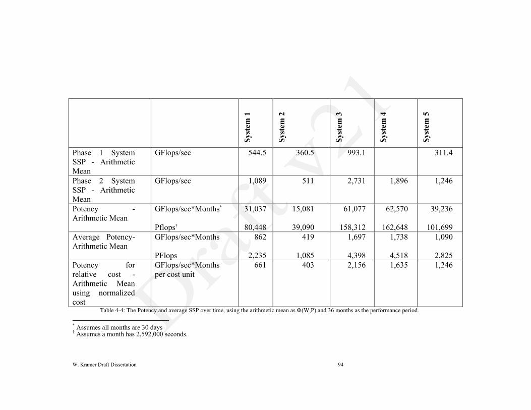
W. Kramer Draft Dissertation 94
Syst
em 1
Syst
em 2
Syst
em 3
Syst
em 4
Syst
em 5
Phase 1 System
SSP - Arithmetic
Mean
GFlops/sec 544.5 360.5 993.1 311.4
Phase 2 System
SSP - Arithmetic
Mean
GFlops/sec 1,089 511 2,731 1,896 1,246
Potency -
Arithmetic Mean
GFlops/sec*Months*
Pflops†
31,037
80,448
15,081
39,090
61,077
158,312
62,570
162,648
39,236
101,699
Average Potency-
Arithmetic Mean
GFlops/sec*Months
PFlops
862
2,235
419
1,085
1,697
4,398
1,738
4,518
1,090
2,825
Potency for
relative cost -
Arithmetic Mean
using normalized
cost
GFlops/sec*Months
per cost unit
661 403 2,156 1,635 1,246
Table 4-4: The Potency and average SSP over time, using the arithmetic mean as (W,P) and 36 months as the performance period.
* Assumes all months are 30 days † Assumes a month has 2,592,000 seconds.

W. Kramer Draft Dissertation 95
Peak vs SSP
0
100
200
300
400
Oct-99 Apr-00 Oct-00 Apr-01 Oct-01 Apr-02
Months since installation
NP
B G
Flop
/s
0
1
2
3
4
5
6
Pea
k TF
lop/
s
Measured SSP Gflop/s Planned SSP System Gflop/s
Planned Peak System Tflop/s Actual Peak System Tflop/s
4.9.2 Risks of Using Peak Performance as A Selection Criteria
There are many reasons why decisions should not be made based on peak
performance, or even benchmarks that closely correlate with peak performance. SSP-
1 was used to evaluate and manage the NERSC-3 system. Watching the system
evolve is an excellent example of SSP being used not only to evaluate and select
systems but also to assess on-going performance, the third purpose of benchmarking.
The NERSC-3 system was delivered in two major phases – with the first phase
consisting of IBM Power 355
(“winterhawk") CPUs and a TBMX56
interconnect
originally planned from Oct 1999 to April 2001. The second phase, planned to start in
April 2001, was one of the first systems with the Power 3+ (“nighthawk”) CPU57
s
connected with the IBM ”colony” High Performance Switch58
. The schedule and
performance levels were agreed upon so the average SSP performance was 155
Figure 4-6: Peak vs. Measured SSP-1 performance

W. Kramer Draft Dissertation 96
GFlops/sec over the first 36 months of the contract. In Figure 4-6, the expected SSP
of the two phases is shown as the dark blue line. The Phase 1 system was to start
production service in Oct 1999 with an SSP of more than 40 GFlops/sec, and it would
be replaced with a Phase 2 system in April 2001 at 238 GFlops/sec. Phase 2 actually
had two sub phases, a and b. The difference between the two sub phases was strictly
software improvements. All the phase 2 hardware was deployed at the beginning of
Phase 2a so the Phase 2a and 2b systems had the same peak performance of 3.5
TFlops/s.
The full potency of performance could not be realized at initial Phase 2 delivery.
The hardware configuration of Phase 2 was a number of 16 CPU SMP nodes, each
with two Colony interconnect adaptors. The Colony HPS switch was the first IBM
interconnect that allowed multiple adaptors in a node. The software to use more than
one adaptor was only planned to be available eight months after the hardware
delivery. The system performance of Phase 2a was limited by the interconnect
bandwidth. NERSC-3 showed significantly increased performance once the second
adaptor was usable, eventually reaching 365 GFlops/sec as the overall SSP. Clearly,
the peak performance parameters of the system did not reflect the actually
performance potency of the system until the software allowed full use of the
interconnect performance.
Figure 4-6 shows another valuable aspect of SSP. Contractually, the Potency
starts accumulating only after system acceptance, which occurred later than expected
for Phase 1 and Phase 2. This was due to various issues, including delays in

W. Kramer Draft Dissertation 97
manufacturing, parts availability and software problems that prevented reliable use of
the system. The acceptance of the Phase 1 system occurred in April 2000 rather than
October 1999 and the acceptance of the Phase 2a system was July 2001 rather than
April 2001. On the other hand, the software to exploit the second adapter was
delivered earlier than the eight-month delay originally expected, arriving in October
2001. The early delivery of the dual plane software provided a measured performance
improvement earlier than planned and partially offset the other delays. The system
configuration was adjusted after Phase 2b acceptance so the average of the SSP did
meet the required 36-month average.
The SSP method gives both the purchaser and the supplier protection. The
supplier has the freedom to adjust the schedule of deliverables and the purchaser is
protected by a guarantee of a agreed upon amount of performance delivered in a
certain time period. The degree of adjustments can be constrained as well. For
example, a purchaser probably does not want all the performance delivered in the last
month of the 3-year period, so there may be limits on when the phases are delivered.
4.10 SSP as an On-Going Measure
As mentioned above, benchmarks can be on-going assessments of systems to help
assure systems continue to operate as expected. In order to be effective as an on-
going performance assessment, benchmarks must be run often enough to provide
enough samples for trend analysis in an on-going assessment*. Running the
benchmarks as a regression test after system changes is one approach – but is limited
* In fact, they need to run often to provide enough samples for variation analysis as discussed in
Chapter 8.

W. Kramer Draft Dissertation 98
in the number of observations that can be obtained. This also means there is little
context to judge significant changes versus random errors. An improvement is
running benchmarks regularly – at least weekly to have an understanding that the
system performs properly. Further, the benchmarks should run alongside the regular
workload as a production job rather than in special circumstances such as on a
dedicated system. This allows a better assessment of what the user community sees
for performance, especially if the benchmark suite is drawn from the application
workload itself. In order to be effective in assessing on-going performance, the
benchmark suite should:
1. Be reflective of the workload itself
2. Be able to run within the normal scheduling parameters of the system
3. Run while the normal workload is running
4. Balance running long enough to assess system performance but short
enough not to consume undue amounts of system resource
Figure 4-7: Runtimes of the SSP-2 component benchmarks over an extended time.
Performance of individual SSP Codes (MF)
0
500
1,000
1,500
2,000
2,500
3,000
10/24/2
003
2/24/2
004
6/24/2
004
10/24/2
004
2/24/2
005
6/24/2
005
10/24/2
005
Dates
Ru
n T
ime
in S
eco
nd
s (s
mal
ler
is b
ette
r)
gtc
madcap
milc
paratec
seam3d

W. Kramer Draft Dissertation 99
Figure 4-7 shows the runtimes of the SSP-2 components over two years on the
NERSC-3/3E. The runs were done several times a week and ran as standard
production jobs. Several insights are notable. First, the runtimes are consistent, with a
few exceptions. . Note the large spike in runtime. For the most part, the runtimes are
within the expected variation of non-dedicated systems. At several points, several of
the codes take longer to run, indicating something on the system may be had a
detrimental impact on performance, particularly since they appear to be clustered in
approximately the same time period. The large spikes are an indicator possibly
something is amiss. Once the trend is noticed, further investigation is probably
needed to determine whether there is a system problem. This data can also be used to
judge the consistency of the system that is discussed in detail in Chapter 7.
Figure 4-8 indicates the composite SSP-2 values over time. The green line is the
required contractual performance negotiated. The graph shows that several times the
actual performance was less than expected. This indicated system issues that were
then corrected to return the system to its expected performance levels.

W. Kramer Draft Dissertation 100
Figure 4-8: SSP validated performance on-going performance of the IBM Power 3 system using SSP-2. The line slight above 600 is the contract required metric.
4.10.1 Guarding Against Performance Degradation – NERSC-3
The NERSC-3, Phase 1 system had a persistent degradation of performance,
measured both by SSP-1 and user applications. The system slowed down by
approximately 5% every month until it was fully rebooted, a process that took close
to 3 hours. A reboot would return the system to the expected performance level. This
improper behavior was only detected because of proactively running the SSP-1
benchmarks. Since the system was in place less than 18 months and it took time to
detect the pattern of gradual loss in performance, it was not possible to definitively
determine the cause of the slowdown before the system was replaced with the Phase 2
system. However, recognizing the degradation meant a work around of rebooting the
system every month was worthwhile.
0
100
200
300
400
500
600
700
800
10/24/2
003
2/24/2
004
6/24/2
004
10/24/2
004
2/24/2
005
6/24/2
005
10/24/2
005
Date
Sy
ste
m S
SP
(G
flo
p/s
)

W. Kramer Draft Dissertation 101
4.11 Validating SSP-4 With a Real Workload
One important question is, “Does the SSP metric reflect the actual workload that
runs on a given system?” This is determined by the careful selection of the
component codes that make up the SPP. Once a year, all the projects at NERSC
submit a proposal for computer time allocation. Since 2004, every project was
required to provide performance data on the application codes they use. The
performance data from running jobs is at scale. A NERSC staff member, David
Skinner, implemented the Integrated Performance Monitor (IPM) tool, to assist users
profiling their applications and collecting the required data. IPM59
provides an
integrated method to collect data from hardware performance counters. The 2006
proposal submissions for NERSC allocations were reviewed to determine the
characteristics of the workload, showing how well the applications ran during
2004/2005.
There were 813 separate performance submissions from 316 different project
submissions that had used NERSC systems in the previous period. A performance
submission is considered unique if the combined project ID, code name, and
concurrency are unique. There were 279 unique submissions reported. NERSC
supports a wide range of science disciplines, and the code submissions reflect that as
well. Table 4-5 compares the amount of time used and the number of performance
data submissions of performance data for applications, both by science discipline.
The percentages are aligned, but not exactly because each science area has different
numbers of applications and projects. The main point of the comparison is that the
performance data covers roughly the same areas as the usage profiles. Since the SSP

W. Kramer Draft Dissertation 102
approximates the actual application performance, even with somewhat of an
underestimation, it is reasonable to assume the SSP reflects the workload.
Science Area Percent of
Computational
Usage in
Allocation Year
(AY) 2005
Percent of
Performance
Submissions
based on Data
from AY 2005
Accelerator Physics 5% 7%
Applied Mathematics, Mathematics
and Computer Science
4% 4%
Astrophysics 12 % 7%
Chemistry 13% 12%
Climate and Environmental Science 8% 7%
Engineering 5% 1%
Fusion Energy 29% 20%
Geosciences 2 % 2%
Life Science 8% 4%
Material Science 9% 30%
Quantum ChrymoDynamics (QCD) 8% 3% Table 4-5: The table comparing the amount of time used by science discipline and the number of performance data
submissions of performance data for applications. The percentages are aligned but not exactly because each science area has different numbers of applications and projects. The main point of the comparison is that the
performance date covers roughly the same areas as the usage profiles.
The performance data submissions and the amount of time used by science
disciplines are consistent. The science areas with the larger usage are also the science
areas with more performance data. Therefore, it is reasonable to use the performance
submissions to make general observations of the overall workload, as is done in Table
4-6.
Table 4-6 compares the SSP and measured performance for the applications on
NERSC‟s most parallel system, Seaborg, which is a 6,756 processor SP-3. The result
of using SSP-1 is an average SSP of 115 MFlop/s per processor on Seaborg and SSP-
2 is 214 MFlop/s per processor. The average actual performance reported by the user
community was 191 MFlop/s per processor. Figure 4-9 shows the number of

W. Kramer Draft Dissertation 103
performance profile submission by discipline area, along with average per processors
performance that were reported.
Data Characteristic Amount
Number of Different Projects 316
Number of Different Submissions 813
Number of Different Submissions based on
Seaborg runs
720
Unique Codes 279
Minimum Concurrency 1
Maximum Concurrency 32,768
Seaborg average reported per processor
performance
191
MFlops/s
SSP-1 per CPU performance 115
MFlops/s
SSP-2 per CPU performance 214
MFlops/s Table 4-6: Summary of performance data reported by science projects running at NERSC.
Figure 4-9: Collected hardware performance data for science discipline areas and the CPU Performance data measured using IPM for over 270 applications.
Comparing the profile data from the NERSC user community with the SSP-1 and
SSP-2 measures indicated the SSP method is a valid estimate of a systems
performance for at least the NERSC workload.
Performance of a Diverse Science Workload on Seaborg
0
50
100
150
200
250
nuclea
r phy
sics
acce
lera
tors
applied
math
astro
phys
ics
chem
istry
clim
ate
CS
engine
ering
enviro
nmen
t
fusion
geos
cien
ces
life s
cien
ce
mat
erials
mat
hQCD
Science Areas
Nu
mb
er
of
sam
ple
s
-
50
100
150
200
250
300
Per
CP
U P
erf
orm
an
ce (
GF
lop
/s)
Number of Codes Reports
Per CPU Performance (Gflop/s)

W. Kramer Draft Dissertation 104
4.12 Chapter Conclusion
This chapter demonstrates different ways the SSP method can be used to assess
and evaluate systems. This method provides the ability to define sustained
performance estimates based on time to solution that are correlated with the actual
workload on the system, yet use much fewer applications. The SSP method has been
refined several times, and with each refinement, the version of the SSP is explained
and assessed. The SSP method is shown to be usable to assure continued system
performance.
The SSP method provides a good overall expectation of potency and value for a
system. It also is attractive to vendors who prefer composite tests instead of discrete
tests. SSP provides realistic assessments of the potency and value of HPC systems.