Sustainable Financing Mechanism for Landscape ...
231
Clemson University Clemson University TigerPrints TigerPrints All Dissertations Dissertations August 2021 Sustainable Financing Mechanism for Landscape Sustainability Sustainable Financing Mechanism for Landscape Sustainability Management: A Systematic Approach to Designing a Payments- Management: A Systematic Approach to Designing a Payments- for-Ecosystem Services (PES) in Santee River Basin Network, for-Ecosystem Services (PES) in Santee River Basin Network, South Carolina South Carolina Julie Carl Ureta Clemson University, [email protected] Follow this and additional works at: https://tigerprints.clemson.edu/all_dissertations Recommended Citation Recommended Citation Ureta, Julie Carl, "Sustainable Financing Mechanism for Landscape Sustainability Management: A Systematic Approach to Designing a Payments-for-Ecosystem Services (PES) in Santee River Basin Network, South Carolina" (2021). All Dissertations. 2848. https://tigerprints.clemson.edu/all_dissertations/2848 This Dissertation is brought to you for free and open access by the Dissertations at TigerPrints. It has been accepted for inclusion in All Dissertations by an authorized administrator of TigerPrints. For more information, please contact [email protected].
Transcript of Sustainable Financing Mechanism for Landscape ...
Clemson University Clemson University
TigerPrints TigerPrints
All Dissertations Dissertations
August 2021
Sustainable Financing Mechanism for Landscape Sustainability Sustainable Financing Mechanism for Landscape Sustainability
Management: A Systematic Approach to Designing a Payments-Management: A Systematic Approach to Designing a Payments-
for-Ecosystem Services (PES) in Santee River Basin Network, for-Ecosystem Services (PES) in Santee River Basin Network,
South Carolina South Carolina
Julie Carl Ureta Clemson University, [email protected]
Follow this and additional works at: https://tigerprints.clemson.edu/all_dissertations
Recommended Citation Recommended Citation Ureta, Julie Carl, "Sustainable Financing Mechanism for Landscape Sustainability Management: A Systematic Approach to Designing a Payments-for-Ecosystem Services (PES) in Santee River Basin Network, South Carolina" (2021). All Dissertations. 2848. https://tigerprints.clemson.edu/all_dissertations/2848
This Dissertation is brought to you for free and open access by the Dissertations at TigerPrints. It has been accepted for inclusion in All Dissertations by an authorized administrator of TigerPrints. For more information, please contact [email protected].
i
SUSTAINABLE FINANCING MECHANISM FOR LANDSCAPE SUSTAINABILITY
MANAGEMENT: A SYSTEMATIC APPROACH TO DESIGNING A PAYMENTS-
FOR-ECOSYSTEM SERVICES (PES) IN SANTEE RIVER BASIN NETWORK,
SOUTH CAROLINA
A Dissertation
Presented to
the Graduate School of
Clemson University
In Partial Fulfillment
of the Requirements for the Degree
Doctor of Philosophy
Forest Resources
by
Julie Carl P. Ureta
August 2021
Accepted by:
Dr. Marzieh Motallebi, Committee Chair
Dr. Robert Fritz Baldwin, Committee Co-Chair
Dr. Steven Seagle
Dr. Michael Vassalos
ii
ABSTRACT
Natural resources provided by the environment through ecosystem services (ES)
are vital in humanity’s survival, economic development, and human well-being. While ES
improves human well-being, the continuous provision of ES is directly dependent on the
ecosystem’s health and integrity. Changing land uses favoring urbanization, and industrial
complexes rather than forests and agricultural land affects the ecosystem’s health; hence,
affecting the continuous provision of ecosystem services. To ensure sustainable
development, conservation programs should be implemented considering both the
stakeholders’ well-being and maintaining the ecosystem’s health and integrity.
This study designs a sustainable financing mechanism known as Payments-for-
Ecosystem Services (PES), which intends to source financial resources to fuel conservation
programs and support sustainable practices ensuring the continuous flow of good quality
ecosystem services to stakeholders in the Santee River Basin Network (SRBN) of South
Carolina (SC). The study developed a systematic approach for designing a PES in SRBN
by: 1) assessing the stakeholders understanding about conservation concepts and programs;
2) analyzing their preference to identify the priority ecosystem and ES to be subject to
conservation programs; 3) quantifying the physical amount of priority ES in SRBN; 4)
estimating the value of community benefits of the priority ES based on stakeholders’
willingness-to-pay; and 5) determining the ecosystem conditions of the land to identify
which land cover affects the ES provision positively and negatively.
Each phase of the systematic process represents a chapter of this dissertation. The
succeeding outputs from each chapter were integrated into a stakeholder-driven process
iii
of developing a PES. A stakeholder-driven approach ensures a PES scheme that is
favorable to the public and achievable for implementation. Picking up from the results,
the primary focus for this PES design is on water quality regulation and wildlife habitat
improvement. The process also revealed how land cover change affects the ES provision
and how sustainable farming practices address these changes. Finally, integrating the
quantification of various ES revealed specific potential subject areas for operationalizing
the PES and critical locations for improving the strategic implementation of conservation
programs.
iv
DEDICATION
Completing a doctoral program is a serious achievement. But completing a doctoral
program while raising a kindergarten and an infant, together with a wife – who is also
completing another doctoral program – amidst a global pandemic, is nothing short of a
miracle. Let this journey be a testimony of the heavenly Father’s greatness and how He
delivers His promise. Hence, I dedicate this dissertation to my father on earth, and may this
be a message to him from my Father in heaven.
“So whether you eat or drink or whatever you do, do it all for the glory of God”
1 Corinthians 10:31
v
ACKNOWLEDGMENTS
While dissertation manuscripts represent the hard work put into a doctoral program,
it cannot ultimately tell the story of its long journey. As the saying goes, this is simply the
“tip of the iceberg.” Much like the awe that we feel in the most amazing things that we see
around us – be it simple or complex – may it be known that none of it would have been
possible if not by the grace of God.
To my dearest adviser Dr. Marzieh Motallebi, you are truly a blessing for my family
and me. My sincerest gratitude to your guidance and unwavering support.
To my “great” mentors Dr. Robert Baldwin, Dr. Steve Seagle, and Dr. Michael
Vassalos. I am genuinely inspired by the intellectual exchanges that we have had. I am very
grateful for the insights, especially on making this research more impactful and the possible
direction as we move forward.
To my colleagues – Jeremy Dertien, Lucas Clay, Sam Cheplick, Hrishita Negi, and
Dr. Daniel Hanks – for the professional and personal support.
For the family and friends in Clemson, South Carolina – the Winship, Ashcraft, Jin,
Li, the whole Clemson Foothills Church, and others I failed to mention. You have been our
home away from home. Thank you for being God’s instrument in showing His glory as we
go through this program.
For the family and friends in the Philippines. You are my inspiration and
motivation, hoping that this ushers new possibilities to help build our country and society.
And finally, to my family – Nanay Jan, Ate Lira, and Likha – you are the reason
for doing what I do. Together is the best place to be.
vi
TABLE OF CONTENTS
Page
TITLE PAGE ................................................................................................................... i
ABSTRACT ..................................................................................................................... ii
DEDICATION ............................................................................................................... iv
ACKNOWLEDGMENTS ............................................................................................... v
LIST OF TABLES ......................................................................................................... ix
LIST OF FIGURES ......................................................................................................... x
AN INTRODUCTION TO PAYMENTS-FOR-ECOSYSTEM
SERVICES (PES) ..................................................................................................... 1
CHAPTER
I. UNDERSTANDING STAKEHOLDERS’ KNOWLEDGE,
AWARENESS, AND PERCEPTION OF
CONSERVATION PROGRAMS IN SOUTH
CAROLINA ............................................................................................. 6
Introduction ............................................................................................. 6
Methodology .......................................................................................... 12
Results .................................................................................................... 15
Discussion .............................................................................................. 27
Recommendations for future work ........................................................ 29
II. USING STAKEHOLDERS’ PREFERENCE FOR
ECOSYSTEMS AND ECOSYSTEM SERVICES AS
AN ECONOMIC BASIS UNDERLYING
STRATEGIC CONSERVATION PLANNING .................................... 31
Introduction ........................................................................................... 31
Methodology .......................................................................................... 37
Results and Discussion .......................................................................... 45
Summary and Conclusion ...................................................................... 58
vii
Table of Contents (Continued)
Page
III. QUANTIFYING THE LANDSCAPE’S ECOLOGICAL
BENEFITS: AN ANALYSIS OF THE EFFECT OF
LAND COVER CHANGE ON ECOSYSTEM
SERVICES ............................................................................................. 63
Introduction ........................................................................................... 63
Materials and Methods ........................................................................... 68
Results ................................................................................................... 77
Discussion ............................................................................................. 86
Conclusion ............................................................................................. 89
IV. VALUATION OF ECOSYSTEM SERVICE
IMPROVEMENTS IN SANTEE RIVER BASIN
NETWORK............................................................................................ 92
Introduction ........................................................................................... 92
Methodology .......................................................................................... 96
Results and Discussion ........................................................................ 109
Summary and Conclusion ................................................................... 123
V. MEASURING ECOSYSTEM CONDITION USING AN
INTEGRATED ECOSYSTEM SERVICE-BASED
SPATIAL ACCOUNTING FRAMEWORK FOR
SUSTAINABLE LANDSCAPE CONSERVATION.......................... 127
Introduction ......................................................................................... 127
Methodology ........................................................................................ 132
Results and Discussion ........................................................................ 141
Conclusion .......................................................................................... 152
VI. PES: A WAY FORWARD ........................................................................ 155
APPENDICES ............................................................................................................. 159
A: Survey questionnaire for knowledge, awareness, and
perception survey ................................................................................. 160
B: Summary statistics of residents' knowledge, awareness, and
perceptions for conservation ................................................................ 166
C: Garrett Ranking Conversion ...................................................................... 168
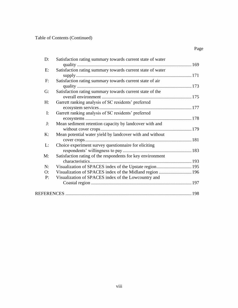
viii
Table of Contents (Continued)
Page
D: Satisfaction rating summary towards current state of water
quality .................................................................................................. 169
E: Satisfaction rating summary towards current state of water
supply ................................................................................................... 171
F: Satisfaction rating summary towards current state of air
quality .................................................................................................. 173
G: Satisfaction rating summary towards current state of the
overall environment ............................................................................. 175
H: Garrett ranking analysis of SC residents’ preferred
ecosystem services ............................................................................... 177
I: Garrett ranking analysis of SC residents’ preferred
ecosystems ........................................................................................... 178
J: Mean sediment retention capacity by landcover with and
without cover crops .............................................................................. 179
K: Mean potential water yield by landcover with and without
cover crops ........................................................................................... 181
L: Choice experiment survey questionnaire for eliciting
respondents’ willingness to pay ........................................................... 183
M: Satisfaction rating of the respondents for key environment
characteristics ....................................................................................... 193
N: Visualization of SPACES index of the Upstate region .............................. 195
O: Visualization of SPACES index of the Midland region ............................ 196
P: Visualization of SPACES index of the Lowcountry and
Coastal region ...................................................................................... 197
REFERENCES ............................................................................................................ 198
ix
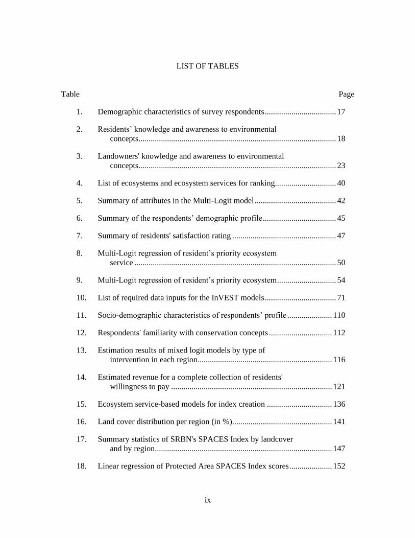
LIST OF TABLES
Table Page
1. Demographic characteristics of survey respondents ................................... 17
2. Residents’ knowledge and awareness to environmental
concepts................................................................................................. 18
3. Landowners' knowledge and awareness to environmental
concepts................................................................................................. 23
4. List of ecosystems and ecosystem services for ranking.............................. 40
5. Summary of attributes in the Multi-Logit model ........................................ 42
6. Summary of the respondents’ demographic profile .................................... 45
7. Summary of residents' satisfaction rating ................................................... 47
8. Multi-Logit regression of resident’s priority ecosystem
service ................................................................................................... 50
9. Multi-Logit regression of resident’s priority ecosystem ............................. 54
10. List of required data inputs for the InVEST models ................................... 71
11. Socio-demographic characteristics of respondents’ profile ...................... 110
12. Respondents' familiarity with conservation concepts ............................... 112
13. Estimation results of mixed logit models by type of
intervention in each region.................................................................. 116
14. Estimated revenue for a complete collection of residents'
willingness to pay ............................................................................... 121
15. Ecosystem service-based models for index creation ................................ 136
16. Land cover distribution per region (in %)................................................. 141
17. Summary statistics of SRBN's SPACES Index by landcover
and by region....................................................................................... 147
18. Linear regression of Protected Area SPACES Index scores ..................... 152
x
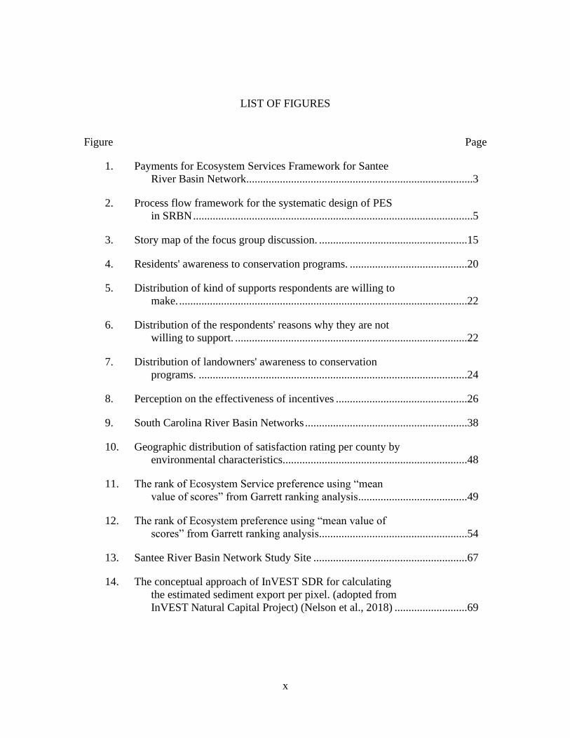
LIST OF FIGURES
Figure Page
1. Payments for Ecosystem Services Framework for Santee
River Basin Network.................................................................................3
2. Process flow framework for the systematic design of PES
in SRBN ....................................................................................................5
3. Story map of the focus group discussion. .....................................................15
4. Residents' awareness to conservation programs. ..........................................20
5. Distribution of kind of supports respondents are willing to
make. .......................................................................................................22
6. Distribution of the respondents' reasons why they are not
willing to support. ...................................................................................22
7. Distribution of landowners' awareness to conservation
programs. ................................................................................................24
8. Perception on the effectiveness of incentives ...............................................26
9. South Carolina River Basin Networks ..........................................................38
10. Geographic distribution of satisfaction rating per county by
environmental characteristics..................................................................48
11. The rank of Ecosystem Service preference using “mean
value of scores” from Garrett ranking analysis .......................................49
12. The rank of Ecosystem preference using “mean value of
scores” from Garrett ranking analysis.....................................................54
13. Santee River Basin Network Study Site .......................................................67
14. The conceptual approach of InVEST SDR for calculating
the estimated sediment export per pixel. (adopted from
InVEST Natural Capital Project) (Nelson et al., 2018) ..........................69
xi
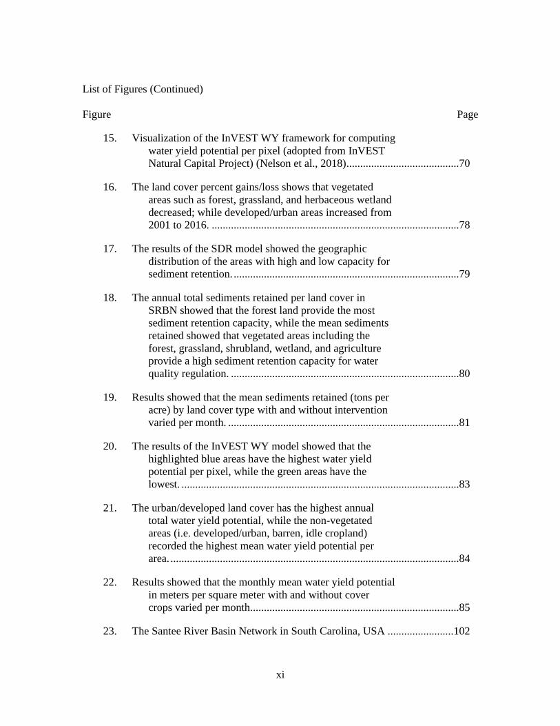
List of Figures (Continued)
Figure Page
15. Visualization of the InVEST WY framework for computing
water yield potential per pixel (adopted from InVEST
Natural Capital Project) (Nelson et al., 2018).........................................70
16. The land cover percent gains/loss shows that vegetated
areas such as forest, grassland, and herbaceous wetland
decreased; while developed/urban areas increased from
2001 to 2016. ..........................................................................................78
17. The results of the SDR model showed the geographic
distribution of the areas with high and low capacity for
sediment retention. ..................................................................................79
18. The annual total sediments retained per land cover in
SRBN showed that the forest land provide the most
sediment retention capacity, while the mean sediments
retained showed that vegetated areas including the
forest, grassland, shrubland, wetland, and agriculture
provide a high sediment retention capacity for water
quality regulation. ...................................................................................80
19. Results showed that the mean sediments retained (tons per
acre) by land cover type with and without intervention
varied per month. ....................................................................................81
20. The results of the InVEST WY model showed that the
highlighted blue areas have the highest water yield
potential per pixel, while the green areas have the
lowest. .....................................................................................................83
21. The urban/developed land cover has the highest annual
total water yield potential, while the non-vegetated
areas (i.e. developed/urban, barren, idle cropland)
recorded the highest mean water yield potential per
area. .........................................................................................................84
22. Results showed that the monthly mean water yield potential
in meters per square meter with and without cover
crops varied per month............................................................................85
23. The Santee River Basin Network in South Carolina, USA ........................102
xii
List of Figures (Continued)
Figure Page
24. Sample choice set with agroforestry as the intervention ............................106
25. Sample choice set with cover crop as the intervention ...............................106
26. Median satisfaction rating of respondents to key
environmental characteristics in their area ...........................................114
27. Range of marginal willingness-to-pay for the improvement
of ecosystem services by region (in dollar values with
95% confidence interval) ......................................................................119
28. Mapping aspect of ecosystem services .......................................................129
29. SEEA Ecosystem Service Accounting process flow ..................................132
30. Process flow for developing the ES index ..................................................135
31. The Santee River Basin Network as study site divided by
region (Upstate, Midland, Lowcountry and Coastal) ............................140
32. ES Index to SPACES Index ........................................................................143
33. Sample pixel values per SPACES Index classification ..............................145
34. Sample conservation area SPACES Index (Congaree
National Park polygon) .........................................................................151
1
AN INTRODUCTION TO PAYMENTS-FOR-ECOSYSTEM SERVICES (PES)
Natural resources provided for by the environment through ecosystem services are vital in
humanity’s survival, economic development, and human well-being. Ecosystem services (ES) are
benefits that people get from the natural environment or the ecosystems (Millenium Ecosystem
Assessment, 2005). Notably, these benefits address human needs and wants in the form of raw
material, protection, recreation, or part of traditional practices. Ecosystem services are classified
into four types: 1) provisioning services such as food, water, raw materials for production; 2)
regulating services such as regulation of flood, climate, or disease; 3) supporting services such as
nutrient cycling and soil formation; and 4) cultural services such as recreational, educational,
spiritual, and other non-material benefits used for traditional practices (Millenium Ecosystem
Assessment, 2005). Furthermore, MEA (2005) defined “well-being” as multi-constitutional,
including basic material for a good life, freedom of choice and action, health, and good social
relations, and security (Millenium Ecosystem Assessment, 2005). Naturally, diverse ecosystems,
which yield varying significant ES, thrive in watersheds. Watersheds host different ecosystems
such as forests, grasslands, aquatic, and agriculture. Therefore, the state of the watershed’s
condition directly affects the quantity and quality of ES.
A watershed is defined as an area of land which drains water, sediments, and dissolved
materials into a common body or outlet, such as any point along a stream channel, the mouth of a
bay area, lake, or reservoir (United States Geological Survey, n.d.). However, increasing demand
for goods and services also leads to rapid urbanization, which threatens the state of the watershed.
Ecosystems from different land use within the watershed are converted to industrial, commercial,
and urbanized zones, resulting in a rapid decline of available natural resources and ES degradation.
2
Hence, conservation practices became critical measures to ensure the continuous provision of
goods and services while preserving a sustained and integral part of ES for future generations.
One of the best management practices of watershed and natural resource management is to
develop a sustainable financing mechanism for priority conservation programs. This mechanism
allows a continuous flow of financial resources to fuel programs towards strategic key
conservation areas and practices, ensuring a constant flow of good quality ES. One sustainable
financing mechanism is widely known as the Payments for Ecosystem Services (PES) scheme. In
this scheme, the ES providers ensure the continuous provision of ecosystem service products by
maintaining healthy ecosystems through conservation practices. While on the other hand, ES
beneficiaries support the ES providers by compensating their efforts to ensure continuous
provision of ecosystem services. Traditionally, PES is defined as: 1) voluntary transaction where;
2) a well-defined ES; 3 is being bought by a minimum of one ES buyer; 4) from a minimum of
one ES provider; and 5) if and only if the ES provider secures ES provision (Wunder, 2005).
However, the critical characteristic for a PES is not simply just that there had been an exchange of
service and money transaction but that the payment causes the benefit to occur (Forest Trends, The
Katoomba Group, & UN Environment Programme (UNEP), 2008). Therefore, the agreement
within a PES scheme should bind both parties into delivering their commitments, such as in an
actual market transaction, making PES a “pseudo-market.” However, the creation of markets
involves a rigorous understanding of fundamental market elements such as demand preferences,
determination of the actual product, quantification of units, and value estimation. Furthermore,
since PES specifically targets conservation areas in a watershed, it is imperative that both
individual and spatial prioritization of ecosystems and ES are considered in the design process.
Therefore, this research develops a systematic approach to designing a PES in the Santee River

3
Basin Network (SRBN) of South Carolina (SC) by identifying the key elements and players in a
PES framework (Figure 1).
Figure 1 Payments for Ecosystem Services Framework for Santee River Basin Network
Precisely, the design should adhere to standards where the PES should be stakeholder-
involved, with established scientifically sound ES linkages, with systematic analysis of the
stakeholders’ capacity to support the program, and identify precise locations for strategic
implementation of the conservation programs. The establishment of a PES in the landscape of
SRBN enhances the ability of development and conservation managers to balance the dynamic
pressures between economic progress and environmental conservation.
The study will be conducted in chapters to systematically develop a PES framework for
SRBN (Figure 2). Chapter 1 of this research analyzes the baseline knowledge, awareness, and
perception of stakeholders of SC. Understanding their baseline information provides critical
4
insight into the potential problems and possible solutions. Essentially, this chapter paints the status
quo in identifying the best approach for establishing the PES and landscape management.
Chapter 2 analyzes SC residents' preference for identifying the priority ecosystems and ES
for conservation program targeting. This also enables understanding the factors that likely affect
their preference and which ES will residents support in the PES scheme.
Chapter 3 picks up the priority ES identified from the previous chapter and quantifies the
amount in physical units produced by the landscape using the Integrated Valuation of Ecosystem
Services and Tradeoffs (InVEST) model. This chapter establishes the direct linkage of the priority
ES to the stakeholders. Furthermore, this also provides information to build a basis for the status
quo about the state of the ES and laying out the geographic picture of the ES’s condition across
the landscape.
Chapter 4 utilizes the information established from Chapters 1 and 2 to estimate SC
residents' value for improving the priority ES. Using a choice experiment approach, a non-market
valuation technique, the study elicits the residents' willingness to pay (WTP) to support sustainable
farming practices, particularly the application of cover crops and implementation of agroforestry
farming. Essentially, this estimates the capacity of the target stakeholders that will be involved in
the PES scheme as ES buyers.
Finally, Chapter 5 integrates the results of Chapter 3 and other ES-based models to develop
an approach that accounts for the ecosystem condition in producing ES in each basic spatial unit
across the landscape. This is done by creating the Spatial Accounting of Ecosystem Services
(SPACES) index, which aggregates each ES-based models' estimated physical quantities into one
performance index score to be stored in each 9m x 9m pixel. The SPACES index's development

5
emphasizes the precise location of pixels across the landscape that could be best included in the
PES scheme.
Figure 2 Process flow framework for the systematic design of PES in SRBN
Principally, this research aims to introduce novel approaches in landscape sustainability
science and management using ecological and economic concepts. While mainstream trend shows
that economic progress typically undermines environmental health, novel approaches such as the
PES and other sustainable financing mechanisms suggest that it is possible that economic progress
and environmental conservation to be achieved simultaneously.
6
CHAPTER ONE
UNDERSTANDING STAKEHOLDERS’ KNOWLEDGE, AWARENESS, AND
PERCEPTION OF CONSERVATION PROGRAMS IN SOUTH CAROLINA1
Introduction
South Carolina (SC) has historically been heavily dependent on natural resources and
agribusiness industry as a primary driver of economic growth and development (Willis & Straka,
2016). The agribusiness industry of SC yields a total annual economic impact of $46.2 billion
which corresponds to 247,000 jobs and $9.6 billion in labor income (Von Nessen, 2020) The state
is a major production hub for timber, corn, cotton, soybean, rice, and peanuts (USDA-NASS,
2019a). However, with the rising economic potential of other industries, the direct economic
contribution from natural resource-based industries is declining dramatically. As of 2017, only
0.5% of the South Carolina’s gross domestic product (GDP) comes from agribusiness and natural
resource-based industries, while 2.4% coming from utilities which includes water distribution. (SC
Department of Employment and Workforce, 2018). On the other hand, a larger amount of the
state’s GDP comes from real estate (13%) (SC Department of Employment and Workforce, 2018).
The increasing popularity of South Carolina as a place to relocate, own a second home, or invest
increases housing prices within the state (South Carolina Realtors, 2019). In addition, cities and
developed areas are expanding to meet the growing demand of the economy and residential
property needs. This makes it financially attractive for landowners to convert their land into
commercial and urbanized zones. From 2001 to 2016, a gradual increase in urban areas can be
observed in land cover maps. Consequently, vegetated areas, including forest land, grassland,
agricultural land, and pasture land are noticeably declining (USGS, n.d.-a). This trend of vegetated
1 Chapter accepted for publication in the Journal of South Carolina Water Resources Center

7
areas being converted to commercial and urban areas is expected to continue along with population
growth and increasing primary value of the land (Sohl & Sayler, 2008) .
While socioeconomic factors typically drive these land cover changes, most often other
benefits and attributed costs are not totally accounted for, including the impacts and benefits from
ecosystems in the form of ecosystem services. Ecosystem services (ES) are processes and products
provide by an environment that affects human well-being (Millenium Ecosystem Assessment,
2005). While ES are mainly classified into four types - provisioning, regulating, supporting, and
socio-cultural ES – most often only the provisioning ecosystem services are accounted for in
economic development (Wunder, 2005). This leads to undervaluation of ecosystem resources
across different land uses, eventually leading to a degradation of ES, and ultimately producing
irreversible damage to the environment (Wunder, 2005). Declines in natural resource land cover
and associated loss of environmental services poses a significant concern to society.
In the attempt to balance economic progress and ecological sustainability, conservation
programs were developed. One approach is to provide incentives or financial support to attract
landowners to conserve all or some portion of their land. These programs are actively promoted
by the United States Department of Agriculture and Natural Resources Conservation Service
(USDA – NRCS) in the form of conservation incentive programs such as the Environmental
Quality Incentives Program (EQIP), Conservation Reserve Program (CRP), and Agricultural
Conservation Easement Program (ACEP) (Mercer, Cooley, & Hamilton, 2011). Other institutions,
such as The Nature Conservancy (TNC), South Carolina Conservation Bank, Ducks Unlimited,
and numerous local and non-profit land trust groups (Land Trust Alliance, n.d.) also promote and
support these programs.

8
Conservation programs are not new in South Carolina. For example, some landowners
allocate parcels of their land as conservation easements while others participate by developing
their land in accordance to the state conservation plans. These measures protect the ecosystems
from degradation and contribute to continuous provision of ES in the process. While these
conservation programs prevent the conversion of vegetated land to urban and developed areas,
they could also be used for improving the ES. This could be done when landowners create more
green and natural areas that contribute to habitat improvement (Barral, 2020; Chiavacci & Pindilli,
2020). In fact, news of habitat improvement in some areas has been reported (Moultrie News,
2019), where farm and forestland protection are continuously promoted through conservation
programs (South Carolina Dept of Natural Resources, 2019).
Although vast areas of land have some form of protection, these protections only cover
roughly 14% of the total area of the state (South Carolina Dept of Natural Resources, 2019). Hence,
additional landowners and farmers have yet to be engaged in conservation programs. Given the
need for enhanced conservation of ES, there is an outstanding question of why landowners and
farmers are not taking advantage of these programs? Tumpach et al. (2018) interviewed loggers
and landowners to understand the barriers for implementing forestry best management practices
in Georgia, USA. They found that landowners prioritize training as the main factor for deciding to
implement forestry best management practices; education and information campaign about the
importance of sustainable forestry should be developed (Tumpach, Dwivedi, Izlar, & Cook, 2018).
Similarly, this could also apply to South Carolina landowners to engage in conservation programs.
On the other hand, since conservation programs are expected to improve the overall quality
of the environment, this improves the ES enjoyed by the residents. While residents do not have the
direct capability to implement conservation strategies, they are typically the final recipients of the

9
ES. Support from the general public can generate significant influence for implementing
conservation strategies and managing protected areas (Calderon, Anit, Palao, & Lasco, 2012;
Thompson, 2018; J.C.P. Ureta, Lasco, Sajise, & Calderon, 2016; Weaver & Lawton, 2008). The
general public’s acceptance of conservation strategies creates social safeguards for critical
ecosystems (McNeely, 1990; Miller & Hobbs, 2002; Shafie, Mod Sah, Abdul Mutalib, & Fadzly,
2017). Furthermore, financial and material support can be generated from the public for ensuring
the sustainability of conservation programs (Bottorff, 2014; Forest Trends et al., 2008; Ingram et
al., 2014; Thompson, 2018; J.C.P. Ureta et al., 2016). Therefore, it is important to understand the
residents’ perception toward these programs. Weaver and Lawton (2008) investigated the
perception of residents in Columbia, South Carolina towards the protection of Congaree National
Park. Their results showed that a majority of the residents perceived that the national park is an
asset and that they have a responsibility to ensure that the park is protected. Furthermore, residents
also expressed that they should have an opportunity to participate in the protection of the park and
provide planning inputs (Weaver & Lawton, 2008). Although there could be a difference in the
perception towards conserving a national park as compared to other conserved land, the results
still indicate that residents would be willing to participate in protecting land that was deemed to
be an asset and contributes to their well-being. Therefore, in terms of conservation programs,
feedback from residents could provide critical insights for successful implementation.
To understand the feasibility, potential gaps, and possible strategies of implementing
conservation programs in South Carolina (SC), we elicited the knowledge, awareness, and
perception of forest landowners and residents towards conservation and conservation programs.
We focused on the landowners’ and residents’ perception as they primarily represent the ES
provider and the ES final recipient, respectively. The data collected by this study could function
10
as a baseline of the perception of both groups towards conservation program implementation.
Furthermore, this study could be used as a feedback mechanism of stakeholders to provide their
insights towards conservation programs.
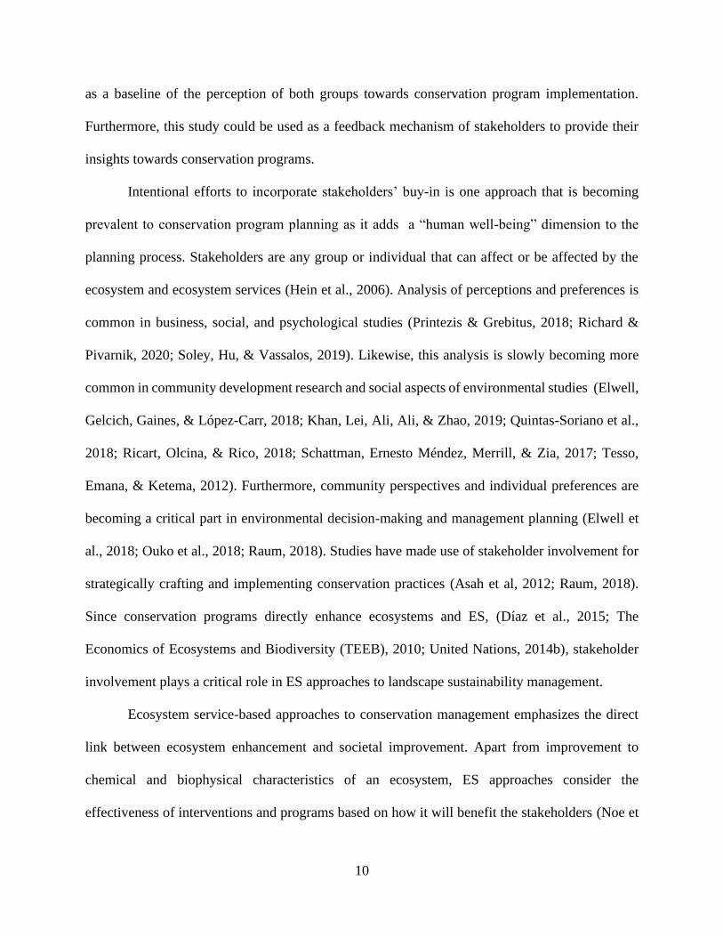
Intentional efforts to incorporate stakeholders’ buy-in is one approach that is becoming
prevalent to conservation program planning as it adds a “human well-being” dimension to the
planning process. Stakeholders are any group or individual that can affect or be affected by the
ecosystem and ecosystem services (Hein et al., 2006). Analysis of perceptions and preferences is
common in business, social, and psychological studies (Printezis & Grebitus, 2018; Richard &
Pivarnik, 2020; Soley, Hu, & Vassalos, 2019). Likewise, this analysis is slowly becoming more
common in community development research and social aspects of environmental studies (Elwell,
Gelcich, Gaines, & López-Carr, 2018; Khan, Lei, Ali, Ali, & Zhao, 2019; Quintas-Soriano et al.,
2018; Ricart, Olcina, & Rico, 2018; Schattman, Ernesto Méndez, Merrill, & Zia, 2017; Tesso,
Emana, & Ketema, 2012). Furthermore, community perspectives and individual preferences are
becoming a critical part in environmental decision-making and management planning (Elwell et
al., 2018; Ouko et al., 2018; Raum, 2018). Studies have made use of stakeholder involvement for
strategically crafting and implementing conservation practices (Asah et al, 2012; Raum, 2018).
Since conservation programs directly enhance ecosystems and ES, (Díaz et al., 2015; The
Economics of Ecosystems and Biodiversity (TEEB), 2010; United Nations, 2014b), stakeholder
involvement plays a critical role in ES approaches to landscape sustainability management.
Ecosystem service-based approaches to conservation management emphasizes the direct
link between ecosystem enhancement and societal improvement. Apart from improvement to
chemical and biophysical characteristics of an ecosystem, ES approaches consider the
effectiveness of interventions and programs based on how it will benefit the stakeholders (Noe et

11
al., 2017). Although there is a growing interest in adopting an ES-based management approach
(Daily et al., 2009), it is not without challenges. Since landowners may have full control in
managing their properties, following a proposed conservation program that enhances ES provision
on the land is only a prerogative for the landowner. Therefore, approaches to attract the landowners
through incentives have become the main market-based driver (Goldman, Thompson, & Daily,
2007; Thompson, 2018; Vedel, Jacobsen, & Thorsen, 2015; Zanella, Schleyer, & Speelman, 2014).
On the other hand, since conservation program interventions are directed towards improving
ecosystems, the effects on society are usually through indirect benefits from ES. Indirect benefits
typically have no market values and are deemed free by the recipients (Wunder, 2005). This leads
to undervaluation and underappreciation of the impacts of the conservation programs to the ES
(Calderon et al., 2012; Doherty, Murphy, Hynes, & Buckley, 2014; Khan & Zhao, 2019; S. Liu,
Costanza, Farber, & Troy, 2010; J.C.P. Ureta et al., 2016). However, since ES transcend private
and political boundaries, conservation across the landscape is a prerequisite for sustainability and
continuous provision of ES. Therefore, for effective implementation of an ES-based approach,
stakeholder buy-in is an important factor (Goldman et al., 2007; Pascual et al., 2014; Thompson,
2018). Implementation of conservation programs concerns both landowners and residents as major
stakeholders. It is for these reasons that diverse stakeholder engagement may play an important
role in planning and evaluating ES strategic interventions.
On one hand, landowners are concerned with how they will directly benefit from the
program, how they can access resources for the conservation program(s), or it may even be that
farmers and landowners are not even aware of these programs (Lackstrom et al., 2018; Ricart et
al., 2018; Tumpach et al., 2018). On the other hand, residents are also concerned with whether
these programs will be effective and eventually affect their well-being; how these programs affect
12
the overall state of ES and the environment they live in; if they have enough information about
these programs; or if these programs will be acceptable to the general public (Elwell et al., 2018;
Thompson, 2018; Weaver & Lawton, 2008). These perspectives from stakeholders could help
define the most appropriate and strategic conservation programs for implementation as well as
provide information on necessary adjustments for policymaking.
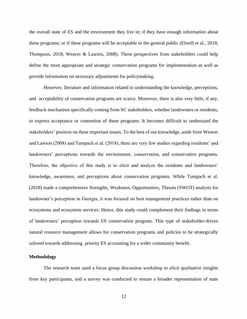
However, literature and information related to understanding the knowledge, perceptions,
and acceptability of conservation programs are scarce. Moreover, there is also very little, if any,
feedback mechanism specifically coming from SC stakeholders, whether landowners or residents,
to express acceptance or contention of these programs. It becomes difficult to understand the
stakeholders’ position on these important issues. To the best of our knowledge, aside from Weaver
and Lawton (2008) and Tumpach et al. (2018), there are very few studies regarding residents’ and
landowners’ perceptions towards the environment, conservation, and conservation programs.
Therefore, the objective of this study is to elicit and analyze the residents and landowners’
knowledge, awareness, and perceptions about conservation programs. While Tumpach et al.
(2018) made a comprehensive Strengths, Weakness, Opportunities, Threats (SWOT) analysis for
landowner’s perception in Georgia, it was focused on best management practices rather than on
ecosystems and ecosystem services. Hence, this study could complement their findings in terms
of landowners’ perception towards ES conservation program. This type of stakeholder-driven
natural resource management allows for conservation programs and policies to be strategically
tailored towards addressing priority ES accounting for a wider community benefit.
Methodology
The research team used a focus group discussion workshop to elicit qualitative insights
from key participants, and a survey was conducted to ensure a broader representation of state
13
resident and landowners’ perceptions and preferences. The survey was tabulated and summarized
for a detailed, quantitative description of stakeholders’ views on these important issues.
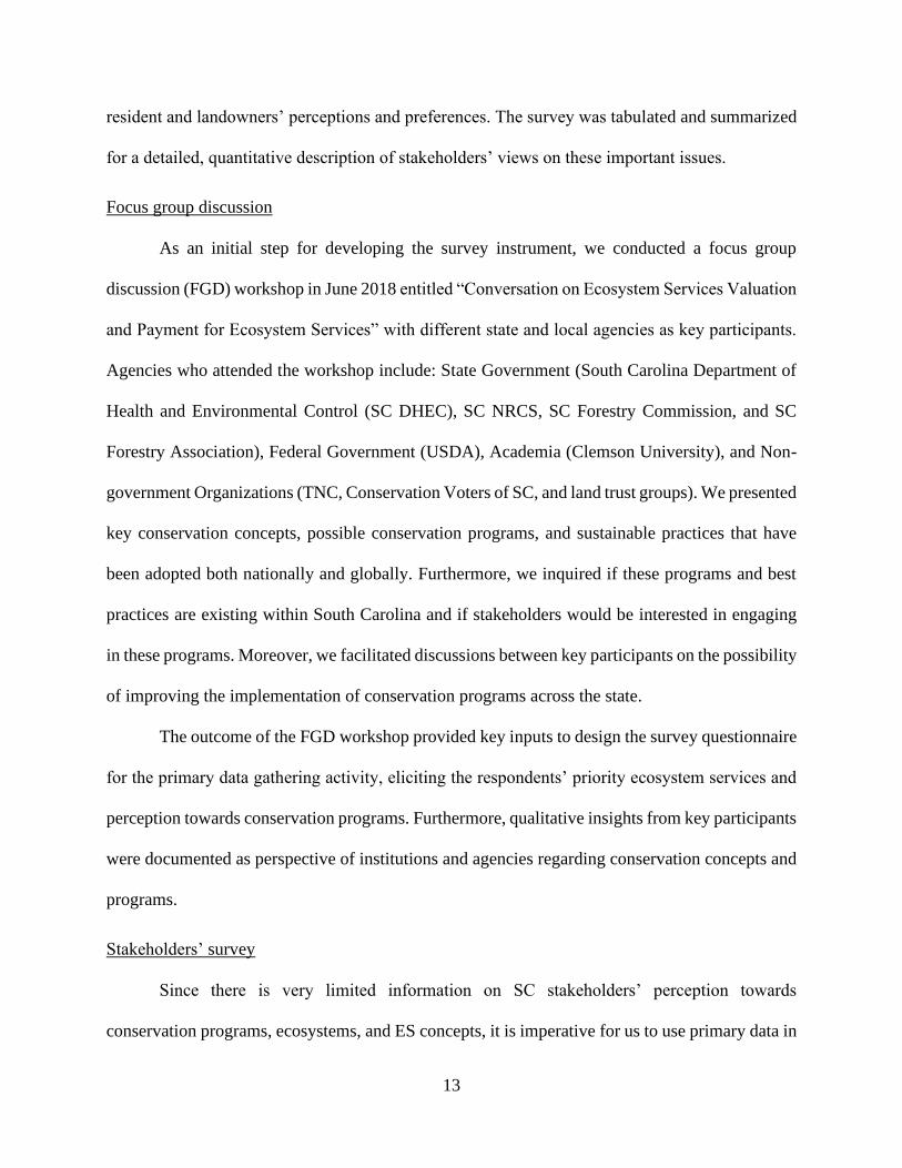
Focus group discussion
As an initial step for developing the survey instrument, we conducted a focus group
discussion (FGD) workshop in June 2018 entitled “Conversation on Ecosystem Services Valuation
and Payment for Ecosystem Services” with different state and local agencies as key participants.
Agencies who attended the workshop include: State Government (South Carolina Department of
Health and Environmental Control (SC DHEC), SC NRCS, SC Forestry Commission, and SC
Forestry Association), Federal Government (USDA), Academia (Clemson University), and Non-
government Organizations (TNC, Conservation Voters of SC, and land trust groups). We presented
key conservation concepts, possible conservation programs, and sustainable practices that have
been adopted both nationally and globally. Furthermore, we inquired if these programs and best
practices are existing within South Carolina and if stakeholders would be interested in engaging
in these programs. Moreover, we facilitated discussions between key participants on the possibility
of improving the implementation of conservation programs across the state.
The outcome of the FGD workshop provided key inputs to design the survey questionnaire
for the primary data gathering activity, eliciting the respondents’ priority ecosystem services and
perception towards conservation programs. Furthermore, qualitative insights from key participants
were documented as perspective of institutions and agencies regarding conservation concepts and
programs.
Stakeholders’ survey
Since there is very limited information on SC stakeholders’ perception towards
conservation programs, ecosystems, and ES concepts, it is imperative for us to use primary data in
14
this study. We used a survey questionnaire, distributed to household residents and landowners by
email, through the Qualtrics electronic platform. To identify between landowners and residents,
landowners are respondents who indicated that they own a secondary property apart from the land
that they currently reside. The electronic platform was used since the majority (79%) of residents
in South Carolina have online access (U.S. Department of Commerce Census Bureau, 2019).
However, since there are still substantial numbers of residents that do not have access to the
internet, the results of this study are only representative of the 79% of the population that has
access to the internet.
A simple random sampling technique was used in the SC residents email database of
Qualtrics to collect responses of 1500 residents. On the other hand, we obtained from the focus
group workshop an email list of 2000 landowners in South Carolina. A link of the Qualtrics survey
was sent to those who were in the list as the landowner respondents.
The survey (Appendix A) had five sections: 1) introduction; 2) knowledge and awareness
towards ecosystems, ecosystem services, and conservation programs; 3) conservation infographic;
4) perception towards ecosystems, ecosystem services, and conservation programs; and 5)
respondents’ demographic profile.
Section 1 of the survey conveyed the background, main objectives, and intention of the
study. Section 2 focused on respondents’ current knowledge of environmental terminologies and
issues. This is critical information as this establishes the knowledge and awareness of the
respondents conservation concepts. Section 3 provided a comprehensive but concise explanation
of environmental terminologies and different conservation programs to ensure that respondents
have the minimum information required to answer the succeeding questions as this will elicit their
choices and decision-making criteria. Section 4 elicited the respondents’ perceptions towards the
15
conservation programs. Finally, Section 5 asked residents about demographics including age,
income bracket, household size, and length of residency in SC.
Results
The study used the insights of the FGD as inputs to the survey questionnaire, while
qualitative accounts from the workshop were used to cross reference against survey results. The
survey results were summarized descriptively to provide information on the types and distribution
of responses.
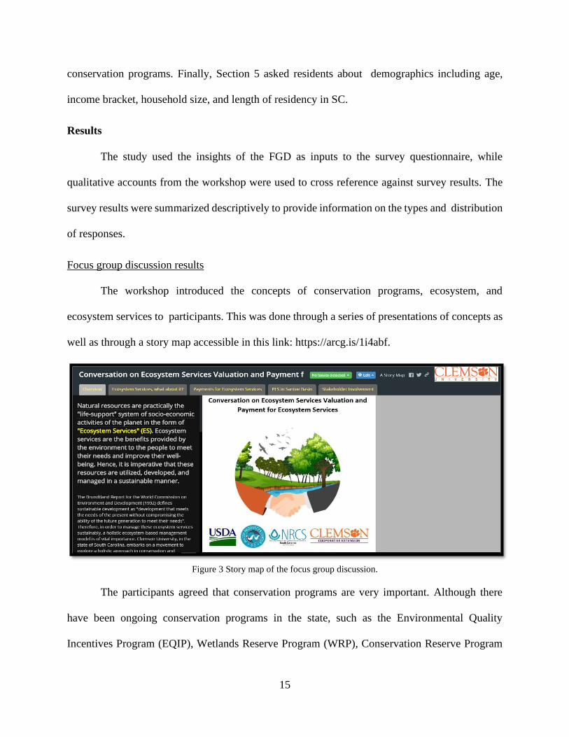
Focus group discussion results
The workshop introduced the concepts of conservation programs, ecosystem, and
ecosystem services to participants. This was done through a series of presentations of concepts as
well as through a story map accessible in this link: https://arcg.is/1i4abf.
Figure 3 Story map of the focus group discussion.
The participants agreed that conservation programs are very important. Although there
have been ongoing conservation programs in the state, such as the Environmental Quality
Incentives Program (EQIP), Wetlands Reserve Program (WRP), Conservation Reserve Program
16
(CRP), and conservation easements through the South Carolina Conservation Bank, these
programs are not fully utilized across the state. Furthermore, there have not been any studies or
evaluation(s) related to why this might be the case. The focus group participants provided expert
opinion on why conservation programs are not fully utilized by stakeholders. Workshop
participants indicated that the low implementation rate of these programs could be associated with
the fact that applications for these conservation programs are often extensive and difficult to
understand. In addition, the logistical difficulty of accessing and implementing conservation
programs is also a significant challenge as stated by landowners that are already part of these
programs. Some farmers and landowners are hesitant to participate due to the impression that their
land management will be strictly regulated. The result of the workshop provided a baseline
impression on the status of conservation programs within the state.
Survey results
In collecting the survey responses, while the total number of surveys distributed was not
disclosed by Qualtrics, the 1500 responses were met by sending out multiple batches of randomly
selected residents from their database using the simple random sampling method. Out of the 1500
accomplished responses, 72 were dropped due to missing data and presence of outliers. Therefore,
1428 responses were used in the analysis of residents’ knowledge, awareness, and perception
towards conservation. Additionally, out of the 2000 list of landowners obtained from the
landowner groups in the focus group workshop, only 228 (11%) responses were received and used
in the analysis.
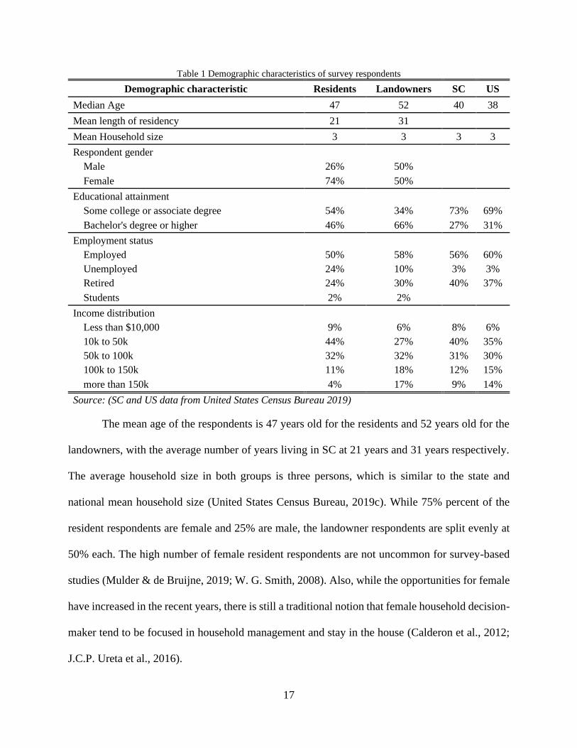
Demographic profile of respondents
Table 1 shows that some of the demographic characteristics of our respondents are
comparable with the state and national data.
17
Table 1 Demographic characteristics of survey respondents
Demographic characteristic Residents Landowners SC US
Median Age 47 52 40 38
Mean length of residency 21 31
Mean Household size 3 3 3 3
Respondent gender
Male 26% 50%
Female 74% 50%
Educational attainment
Some college or associate degree 54% 34% 73% 69%
Bachelor's degree or higher 46% 66% 27% 31%
Employment status
Employed 50% 58% 56% 60%
Unemployed 24% 10% 3% 3%
Retired 24% 30% 40% 37%
Students 2% 2%
Income distribution
Less than $10,000 9% 6% 8% 6%
10k to 50k 44% 27% 40% 35%
50k to 100k 32% 32% 31% 30%
100k to 150k 11% 18% 12% 15%
more than 150k 4% 17% 9% 14%
Source: (SC and US data from United States Census Bureau 2019)
The mean age of the respondents is 47 years old for the residents and 52 years old for the
landowners, with the average number of years living in SC at 21 years and 31 years respectively.
The average household size in both groups is three persons, which is similar to the state and
national mean household size (United States Census Bureau, 2019c). While 75% percent of the
resident respondents are female and 25% are male, the landowner respondents are split evenly at
50% each. The high number of female resident respondents are not uncommon for survey-based
studies (Mulder & de Bruijne, 2019; W. G. Smith, 2008). Also, while the opportunities for female
have increased in the recent years, there is still a traditional notion that female household decision-
maker tend to be focused in household management and stay in the house (Calderon et al., 2012;
J.C.P. Ureta et al., 2016).

18
In regard to highest educational attainment, the majority of resident respondents (54%) had
some college, an associate degree, or lower, which follows the distribution in the state and national
data. On the other hand, the majority of the landowner respondents (66%) have bachelor’s degree
or higher. In terms of the employment status, both resident and landowner respondents have almost
similar distribution with the state and national census data where majority of the population are
employed. Finally, in terms of income distribution, resident respondents have a similar distribution
with state and national data while landowner respondents showed an opposite trend. Forty-seven
percent of the resident respondents have income equal or higher than the state’s median household
income of $51,015, while at least 9% of the respondents fall under the poverty threshold of $20,212
for a family of 3 people (United States Census Bureau, 2019c). On the other hand, 67% of the
landowner respondents have income equal or higher than the state’s median household income
while at least 6% falls under the poverty threshold. Overall, results show that the demographic
characteristics of the residents in this survey is comparable to the state and national statistics. This
indicates that the respondent profile are representative of the overall resident population in SC.
Understanding residents’ perceptions
Residents’ knowledge and awareness of conservation concepts
We asked a series of questions pertaining to conservation concepts and conservation
programs to assess residents’ awareness and baseline knowledge of the topic. The results are
shown in Table 2.
Table 2 Residents’ knowledge and awareness to environmental concepts.
N = 1428 Yes % No %
Familiarity to natural resource conservation 59% 41%
Familiarity to meaning of a watershed 54% 46%
Familiarity to Ecosystem Services 47% 53%
Awareness that air, water, and food come from nature 93% 7%
Awareness that different land uses affect the value of the residence 84% 16%

19
Awareness that ecosystems affect human well-being 87% 13%
Perception if healthy environment is important 97% 3%
Perception if healthy environment includes good quality of water 96% 4%
Perception if healthy environment contributes to abundance of usable water 88% 12%
Perception if healthy environment provides good quality of life in general 97% 3%
Is the term “conservation” the same with the term “preservation”? 63% 9%
Awareness about conservation programs 40% 60%
Results show that respondents understand how the environment is providing environmental
services and improves their well-being. This is evident from the high “Yes” response rate on the
awareness and perception questions, particularly from descriptive statements. However, when
asked about similar concepts using relatively technical terminology such as familiarity with the
meaning of a watershed, ecosystem services or natural resource conservation, only around half of
the respondents answered “yes” to these questions. It is interesting to note that although only 47%
of the respondents are familiar with the term “ecosystem services” yet almost everyone perceives
that a healthy environment is necessary for the provision of water and maintaining good quality of
life. This emphasizes the disconnect between the use of technical terminology and the level of
understanding of the residents about the importance of these concepts. Moreover, when asked to
differentiate between the concepts of preservation and conservation, the majority of respondents
(63%) indicated these concepts are similar. Only 9% said the two concepts are different with the
remaining 28% not able to determine if they are similar or different. Finally, when asked if they
are aware of conservation programs, only 39% said “Yes,” indicating that majority of the residents
are not aware of these programs.
We also showed them a list of different conservation programs that are currently funded
by the US Department of Agriculture (USDA). The distribution of residents that are aware about
these conservation programs within the 39% who said “Yes” are shown in Figure 4 (see Appendix
B).
20
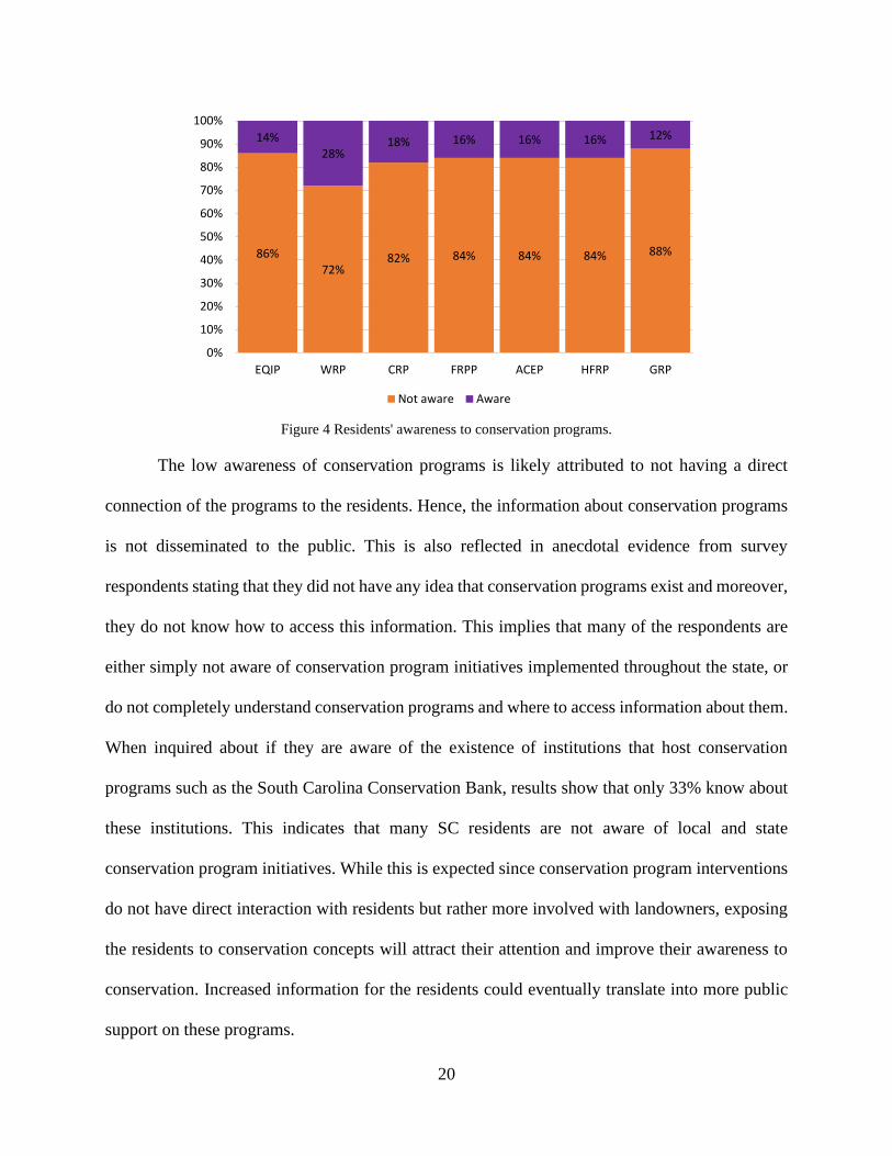
Figure 4 Residents' awareness to conservation programs.
The low awareness of conservation programs is likely attributed to not having a direct
connection of the programs to the residents. Hence, the information about conservation programs
is not disseminated to the public. This is also reflected in anecdotal evidence from survey
respondents stating that they did not have any idea that conservation programs exist and moreover,
they do not know how to access this information. This implies that many of the respondents are
either simply not aware of conservation program initiatives implemented throughout the state, or
do not completely understand conservation programs and where to access information about them.
When inquired about if they are aware of the existence of institutions that host conservation
programs such as the South Carolina Conservation Bank, results show that only 33% know about
these institutions. This indicates that many SC residents are not aware of local and state
conservation program initiatives. While this is expected since conservation program interventions
do not have direct interaction with residents but rather more involved with landowners, exposing
the residents to conservation concepts will attract their attention and improve their awareness to
conservation. Increased information for the residents could eventually translate into more public
support on these programs.
86%72%
82% 84% 84% 84% 88%
14%28%
18% 16% 16% 16% 12%
0%
10%
20%
30%
40%
50%
60%
70%
80%
90%
100%
EQIP WRP CRP FRPP ACEP HFRP GRP
Not aware Aware
21
When asked if they think it will be beneficial for the state’s overall environment and human
well-being to have conservation programs, the majority of the respondents answered “yes” with
86% and 83% distribution, respectively. Furthermore, the majority of the respondents, 90% and
92%, agree that the state should lead conservation efforts and that the public has a significant role
in conservation, respectively. Additionally, when asked about which level of government should
be responsible for managing conservation areas, 38% said that this should be a shared
responsibility between federal, state, local government, as well as the public; while 28% believe
this should be the sole responsibility of the state government. A small group (13%) said
conservation should be the responsibility of private institutions, 7% said it should be the sole
responsibility of the local government, 5% indicated the federal government, while the remaining
respondents said non-governmental organizations should have this role.
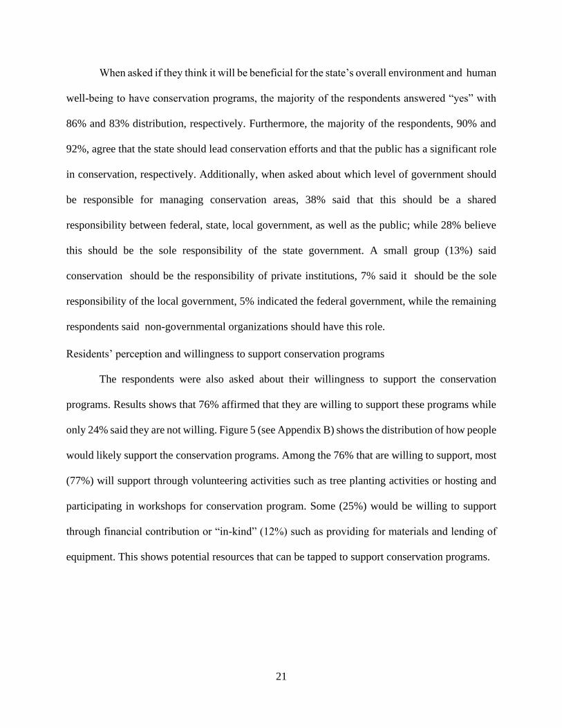
Residents’ perception and willingness to support conservation programs
The respondents were also asked about their willingness to support the conservation
programs. Results shows that 76% affirmed that they are willing to support these programs while
only 24% said they are not willing. Figure 5 (see Appendix B) shows the distribution of how people
would likely support the conservation programs. Among the 76% that are willing to support, most
(77%) will support through volunteering activities such as tree planting activities or hosting and
participating in workshops for conservation program. Some (25%) would be willing to support
through financial contribution or “in-kind” (12%) such as providing for materials and lending of
equipment. This shows potential resources that can be tapped to support conservation programs.
22
Figure 5 Distribution of kind of supports respondents are willing to make.
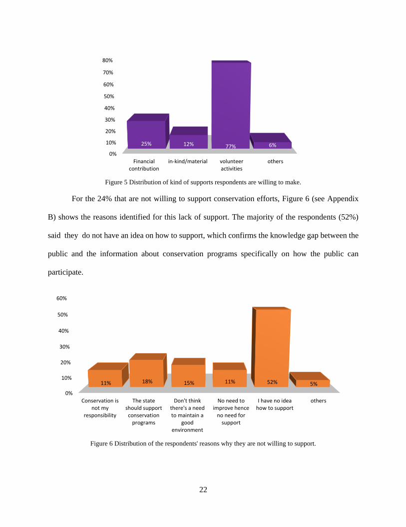
For the 24% that are not willing to support conservation efforts, Figure 6 (see Appendix
B) shows the reasons identified for this lack of support. The majority of the respondents (52%)
said they do not have an idea on how to support, which confirms the knowledge gap between the
public and the information about conservation programs specifically on how the public can
participate.
Figure 6 Distribution of the respondents' reasons why they are not willing to support.
0%
10%
20%
30%
40%
50%
60%
70%
80%
Financialcontribution
in-kind/material volunteeractivities
others
25% 12% 77% 6%
0%
10%
20%
30%
40%
50%
60%
Conservation isnot my
responsibility
The stateshould supportconservation
programs
Don't thinkthere's a needto maintain a
goodenvironment
No need toimprove hence
no need forsupport
I have no ideahow to support
others
11% 18% 15% 11% 52% 5%
23
Finally, we also asked respondents on their position if they would agree for the state to
fund for conservation programs using state funding. A large majority of the respondents (76%)
agreed, while very few (7%) disagree and the remaining (17%) chose not to respond. This indicates
that, if given enough information, residents could be willing to support conservation programs in
the state. While the residents do not necessarily have control over how the state funds are spent,
their willingness to support could be used as leverage to encourage representatives and
policymakers in increasing the available funds for supporting the implementation of conservation
programs.
Understanding landowners’ perspective
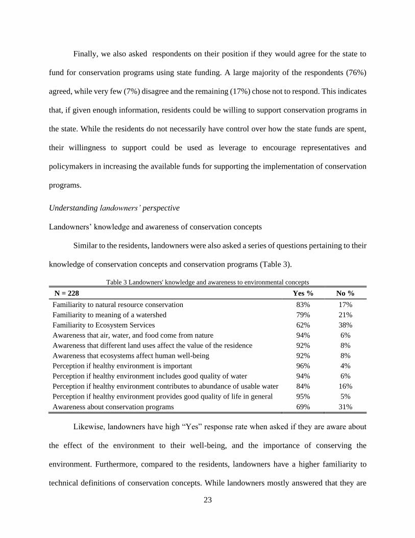
Landowners’ knowledge and awareness of conservation concepts
Similar to the residents, landowners were also asked a series of questions pertaining to their
knowledge of conservation concepts and conservation programs (Table 3).
Table 3 Landowners' knowledge and awareness to environmental concepts
N = 228 Yes % No %
Familiarity to natural resource conservation 83% 17%
Familiarity to meaning of a watershed 79% 21%
Familiarity to Ecosystem Services 62% 38%
Awareness that air, water, and food come from nature 94% 6%
Awareness that different land uses affect the value of the residence 92% 8%
Awareness that ecosystems affect human well-being 92% 8%
Perception if healthy environment is important 96% 4%
Perception if healthy environment includes good quality of water 94% 6%
Perception if healthy environment contributes to abundance of usable water 84% 16%
Perception if healthy environment provides good quality of life in general 95% 5%
Awareness about conservation programs 69% 31%
Likewise, landowners have high “Yes” response rate when asked if they are aware about
the effect of the environment to their well-being, and the importance of conserving the
environment. Furthermore, compared to the residents, landowners have a higher familiarity to
technical definitions of conservation concepts. While landowners mostly answered that they are

24
familiar and aware of the environmental characteristics, it is interesting to note that using the term
“Ecosystem Services” is still relatively uncommon since only 62% of the landowner respondents
answered that they are familiar to ES. This indicates that, although landowners are more familiar
with the technical jargon used in conservation concepts, effectively communicating conservation
concepts is still a high priority, particularly those concepts that are emerging and relatively new.
Furthermore, when asked if they are aware of conservation programs, majority (69%) said that
they are aware.
Landowners’ perception on conservation programs and its management
We also showed the landowners a list of federal government conservation programs to
know how many of them are familiar of these. Results in Figure 7 (see Appendix B) show that
even with the landowner respondent groups who are aware that there are conservation programs
available, the majority are still not aware of these specific listed federal programs.
Figure 7 Distribution of landowners' awareness to conservation programs.
Similar to the residents, landowners have limited information on accessing these
conservation programs. Furthermore, anecdotal evidence from the respondents’ comments
88%76%
82% 85% 85% 87% 92%
12%24%
18% 15% 15% 13% 8%
0%
10%
20%
30%
40%
50%
60%
70%
80%
90%
100%
EQIP WRP CRP FRPP ACEP HFRP GRP
Not aware Aware

25
particularly said that they do not know the specifics on how to access these conservation programs.
However, when asked if they are aware of the SC Conservation Bank, majority (59%) responded
“Yes”. This indicates that landowners may be more familiar with local conservation programs such
as conservation easements rather than the federal programs.
Landowners were also asked if they think conservation programs are beneficial for the
state’s overall environment and human well-being. Eighty-nine percent of the respondents
indicated that they are beneficial for the state while 81% acknowledged that they are beneficial to
human well-being.
When asked about the appropriate conservation program managers, 85% indicated that it
should be the state that should take leadership in conserving its natural resources. Yet when asked
which institution should primarily support the conservation programs, 29% said that it should be
a shared responsibility between the federal, state, and local government. Furthermore, 26% said
that it should be a private responsibility, 18% said that it should be the state government alone,
11% prefer the federal government alone, and the rest is through non-profit organizations and local
governments. However, when asked if they think the public has a role in conservation, 91% of the
respondents answered “Yes”. This suggests that respondents know that they have a sense of
responsibility in taking care of the environment.
Landowners’ willingness to participate in conservation programs
Specifically, for the landowners, we elicited their preference if they will be willing to
support and participate in conservation programs. The majority (85%) of the landowners are
willing to support the implementation of conservation programs within the state. However, while
a substantial amount (46%) are willing to participate in conservation programs even without
26
compensation, this improves significantly (75%) when there is an option to support and get
compensated at the same time.
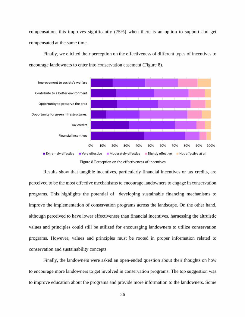
Finally, we elicited their perception on the effectiveness of different types of incentives to
encourage landowners to enter into conservation easement (Figure 8).
Figure 8 Perception on the effectiveness of incentives
Results show that tangible incentives, particularly financial incentives or tax credits, are
perceived to be the most effective mechanisms to encourage landowners to engage in conservation
programs. This highlights the potential of developing sustainable financing mechanisms to
improve the implementation of conservation programs across the landscape. On the other hand,
although perceived to have lower effectiveness than financial incentives, harnessing the altruistic
values and principles could still be utilized for encouraging landowners to utilize conservation
programs. However, values and principles must be rooted in proper information related to
conservation and sustainability concepts.
Finally, the landowners were asked an open-ended question about their thoughts on how
to encourage more landowners to get involved in conservation programs. The top suggestion was
to improve education about the programs and provide more information to the landowners. Some
0% 10% 20% 30% 40% 50% 60% 70% 80% 90% 100%
Financial incentives
Tax credits
Opportunity for green infrastructures.
Opportunity to preserve the area
Contribute to a better environment
Improvement to society's welfare
Extremely effective Very effective Moderately effective Slightly effective Not effective at all
27
also suggested to partner with community organizations such as local churches and clubs as venue
for disseminating the information. Additionally, some also suggested to have a proper and
transparent planning for implementing the conservation programs. A common contention among
landowners’ responses was the impression that getting involved in the conservation programs is
as if allowing the government to dictate and control what can be done in the land. Therefore,
working closely with landowners, especially by including them in the decision-making process
and in crafting the conservation plans, could improve their engagement to the program.
Discussion
This study assessed the knowledge, awareness, and perception of South Carolina
stakeholders towards conservation concepts, conservation programs, and concepts of ecosystems
and ecosystem services. A summary of survey results highlight that residents have a high
awareness and knowledge of ecosystems and ecosystem services concepts, particularly if
discussed using widely common terminologies such as nature, food, air, water, and environment.
Residents mostly agree that proper management of ecosystems and ecosystem services through
conservation programs are important. However, this affirmation declines when jargon and
technical terminology such as “watershed” and “ecosystem services” are used when
communicating with residents. Furthermore, while landowners seem to have more familiarity in
conservation concepts, the use of technical terminology, particularly “ecosystem services,”
revealed difficulty in understanding conservation concepts. However, since these are key
terminologies in conservation concepts and sustainable development, There appears to be a need
to improve stakeholder communication and information dissemination to ensure that messages
about conservation are properly relayed to stakeholders. A lack of understanding and knowledge
of key concepts reinforces the potential of information disconnect within stakeholders’ current
28
understanding of conservation concepts. This poses a potential issue where there is a
communication deficiency between the scientific community and the stakeholders that are present.
One of the ways to address this is to focus on conservation program information outreach. Using
different mediums such as infographics and video advertisements to promote conservation
concepts will attract stakeholders to be familiar with these programs. Furthermore, it is also
possible that with targeted communication and information, stakeholders can gain the knowledge
they need to make informed decisions. Since many conservation concepts uses technical jargons,
then there is a need to improve this aspect of the challenge.
Furthermore, the study also showed that, although stakeholders have high appreciation for
conservation and improvement of the environment, awareness of conservation programs is limited
both to the residents and the landowners. Specifically, federally instituted conservation programs
seem to be having difficulty in reaching the landowners. Therefore, the accessibility to information
on conservation programs and sustainable practices should be improved both for the landowners
and residents. While residents do not have a direct implementation or operational capacity for the
conservation programs, it will still be beneficial in order garner support from the public. This could
be an opportunity for conservation agencies in promoting conservation programs and strategies
that can gather support from stakeholders since there is already high awareness on the importance
of healthy environment.
Contrary to the impression of conservation managers that stakeholders are hesitant to adopt
conservation programs, the survey results show that the disconnect is likely because of insufficient
information communicated to stakeholders. In fact, the majority of landowners and residents
agreed and responded that they are willing to support conservation programs since these programs
are perceived to have a positive impact on their well-being. However, the percentage of
29
stakeholders who are aware about the specific conservation programs is low. Hence, this could be
an opportunity for improvement for promoting and implementing conservation programs.
Finally, specifically about the perception of the landowners, majority of the landowners
are willing to support and participate the conservation programs. The results show that in order to
encourage more landowners to be involved, tangible incentives such as financial compensation
and tax credits could be used as financing mechanism. However, while incentives are the best way
to encourage landowners to join the program, their values and outlook towards the importance of
the conservation concepts and ecological integrity could still be used to promote the movement.
And a substantial factor for developing values and principles is to have proper and correct
information about the subject, hence the need to improve the communication of conservation
concepts to the stakeholders.
Recommendations for future work
The use of perception surveys to evaluate the stakeholders’ knowledge, perceptions, and
preferences towards conservation concepts and programs could serve as a critical feedback
mechanism for strategizing effective creation and implementation of conservation programs.
Moreover, future work could improve this study by eliciting the perception of stakeholders that do
not have internet access. Utilizing the stakeholders’ perception to develop applied research efforts
related to improving effective information and communication appears to be most critical first
step. Furthermore, the initial insights from these surveys could be a step towards developing more
advanced economic studies such as valuation to support policy making and development of
sustainable financing mechanism for conservation. Working closely with scientists, environmental
managers and policymakers to develop strategic planning initiatives that improve the

30
implementation and success of conservation programs is important for the State’s environmental
health and overall quality of life.

31
CHAPTER TWO
USING STAKEHOLDERS’ PREFERENCE FOR ECOSYSTEMS AND ECOSYSTEM
SERVICES AS AN ECONOMIC BASIS UNDERLYING STRATEGIC CONSERVATION
PLANNING2
Introduction
Ecosystems services (ES), commonly defined as material and non-material benefits that
people receive from the environment (Millenium Ecosystem Assessment, 2005), affect the
economy and eventually improve society’s well-being. Specifically, the provision of ES directly
improve society’s well-being in five dimensions: (1) basic material for a good life, (2) freedom of
choice, (3) health, (4) good social relations, and (5) security (Millenium Ecosystem Assessment,
2005; United Nations, 2014b; Wu, 2013).
While ES improve societal well-being, their continuous provision is directly dependent on
the ecosystem’s health and integrity. This reciprocal relationship is the fundamental basis of
Social-Ecological Systems (SES) or coupled human-environment systems (CHES) (Wu, 2013).
Social-ecological systems’ components are focused on people and other organisms using the
ecosystem services as the main linkage. This complex system is not merely a summation of
“social” and “ecological” systems, as it develops numerous unique characteristics commonly
referred to as emergent properties (Cumming, 2011). Since SES are systems of people and nature,
it follows that humans should be seen as part of nature, and nature should be seen as part of society
(Berkes & Folke, 2000). The SES framework may be central in pursuing sustainability and
resiliency across the landscape. While the goal of sustainability is centered on improving human
well-being (Brundtland, 1987), this cannot be achieved without protecting ecosystems (Wu, 2013).
2 Chapter has been published in Heliyon Journal of 2020. https://doi.org/10.1016/j.heliyon.2020.e05827

32
Therefore, new methodologies that integrate both the social and ecological aspects are being
explored, such as the ES-based approach (Asah et al., 2012; Díaz et al., 2015; Raum, 2018).
The basic foundation of the ES-based approach is that human and ecological well-being
are tightly connected to the sustainable management of resources (Tallis & Polasky, 2009). Apart
from the improvement to the chemical and biophysical characteristics of an ecosystem, the ES-
based approach measures the effectiveness of interventions and programs by considering the
benefits that stakeholders derive from the ecosystem. Notably, improvement of human well-being
is a core principle for an ES approach (Millenium Ecosystem Assessment, 2005). Consequently,
scholars have focused on evaluating consumers’ preferences and welfare impact from the changes
of ES.
Improvement of ES provides a variety of societal benefits. For instance, the application of
green spaces and green infrastructures improves the urban environment while also contributing to
flood mitigation, water quality improvement, and microclimate provision. These regulating
ecosystem services contribute to human health by lowering human exposure to contaminated
floodwaters, removing toxicants, trapping contaminants, and mitigating extreme temperatures
(Summers, Smith, Fulford, & Crespo, 2018). Socio-cultural ecosystem services also provide
multiple benefits, such as therapeutic benefits and heritage benefits (Schmidt, Sachse, & Walz,
2016). Besides, since one ecosystem service typically has a synergistic effect with other ecosystem
services, the impacts of the socio-cultural ecosystem services also affect other types of ecosystem
services (Schmidt et al., 2016).
In contrast, land-use changes that favor urban expansion and industrialization negatively
affect ecosystems, resulting in degradation and decline of ecosystem services (Huang, Zhan, Yan,
Wu, & Deng, 2013; Krkoška lorencová, Harmáčková, Landová, Pártl, & Vačkář, 2016; Y. Liu, Li,
33
& Zhang, 2012; Motoshita, Ono, Finkbeiner, & Inaba, 2016). While it has a negative impact on
human well-being, the decline of the ecosystem services is being overshadowed by the potential
economic gains of these land-use changes. To assess if the ES's foregone benefit is comparable to
the economic gains, several indexes and metrics have been utilized in the literature (Leviston,
Walker, Green, & Price, 2018; Olander et al., 2018; Schmidt et al., 2016; Wainger & Mazzotta,
2011). Although these metrics provide a general understanding of ecosystem services benefits,
identifying which particular social benefit is still not commonly understood (Schmidt et al., 2016).
Other research endeavors focus on evaluating residents’ Willingness to Pay (WTP) to
support water quality improvement (Calderon et al., 2012; Doherty et al., 2014; Khan & Zhao,
2019; J.C.P. Ureta et al., 2016). A consensus across these studies is that residents have a higher
willingness to pay (WTP) for good water quality (Doherty et al., 2014; Khan et al., 2019) and
prefer water quality improvements more than water distribution (Khan & Zhao, 2019). However,
divergence exists. For example, studies at the local scale also show that habitat and recreational
ecosystem services are valued more in certain areas (Castro, Vaughn, García-Llorente, Julian, &
Atkinson, 2016). A study in the United States found that there is a homogeneous distribution of
WTP for the improvement of water quality across the nation. At the same time, it may vary across
different geographic locations for other ecosystem services (Aguilar, Obeng, & Cai, 2018).
Furthermore, residents who are willing to preserve the environmental quality within the watershed
typically relate their WTP to water quality improvement (Brox, Kumar, & Stollery, 1996).
Although literatures regarding understanding stakeholder preference are available mainly on the
topic of willingness-to-pay and welfare economics, there is limited research, particularly on
ecosystem and ecosystem service preference used for conservation planning at a state level.
Furthermore, WTP approaches are prone to large confidence intervals which gives plenty of room

34
for uncertainty (Brent, Gangadharan, Lassiter, Leroux, & Raschky, 2017). While WTP estimates
are useful information for policy-makers, it should only be one of the multiple inputs to be
considered (Brent et al., 2017). Valuation methods may provide a definitive and robust case to
consider the ecosystem services in the decision-making process, but it is essential to understand
the limitations. It does not entirely capture the full values for many non-use services, and the
estimated values are often non-transferable to other sites since no market is involved (Wainger &
Mazzotta, 2011). Hence, other approaches to decision-making need to be considered. Qualitative
accounts, multi-criteria methods, and preferential ranking analysis also provide a different
perspective in understanding people’s perception in the social and environmental context
(Goldman et al., 2007; Thompson, 2018). Since the relationship between people’s perception and
their social-environmental context is complex, this highlights the importance of considering
perception in crafting more effective and inclusive landscape management strategies (Quintas-
Soriano et al., 2018). The use of stakeholder preference and perception is effective in formulating
policies for ecosystem service and natural resource conservation (Quintas-Soriano et al., 2018) and
as a guide for modeling and management efforts (Elwell et al., 2018).
Despite the growing interest in adopting an ES-based management approach (Daily et al.,
2009), their implementation is challenging for several reasons. Land managers should have the
capacity to perform ES analyses and the statutory authority over the land to conduct these
approaches (Noe et al., 2017). Furthermore, practitioners of ES-based management approaches
also have to have the legal mandate to integrate ES in their analyses (Presnall, López-Hoffman, &
Miller, 2015). Also, even with strong statutory support, an unclear understanding of the concept
of ES among stakeholders limits the capacity to perform ES-based analyses (Sitas, Prozesky, Esler,
& Reyers, 2014). In the Southern US, since the majority of forest area is privately owned (Butler

35
& Wear, 2013; South Carolina Forestry Commission, 2015), implementation of ES is even more
challenging. For example, landowners need to voluntarily implement the intervention. Otherwise,
an incentive mechanism has to be developed to attract landowners. One way to address these
challenges is by doing a “bottom-up” stakeholder-based approach to tailor-fit programs based on
the stakeholders’ preference and perception (Ernst & van Riemsdijk, 2013; Raum, 2018; Ricart
Casadevall, 2016; Song & Hu, 2019; Zoderer, Tasser, Carver, & Tappeiner, 2019).
Stakeholders’3 perceptions play an important role in strategically selecting interventions
(Asah et al., 2012; Raum, 2018). The literature on assessing water users’ perspectives typically
focuses on large groups and intermediate consumers, such as farmers and landowners. Although
this approach has provided significant insights and advanced stakeholder involvement for selecting
interventions, the final stakeholder recipients of ES (typically household residents) are less often
consulted regarding their preference (Khan & Zhao, 2019; Pellett & Walker, 2018; Quintas-
Soriano et al., 2018; Ricart et al., 2018; Tumpach et al., 2018). Not accounting for the residents'
perspective as the final recipient of the ES could result in a misalignment in the implementation
of policies for conservation.
This study is an effort to fill this gap in the literature. Specifically, we aim to examine
South Carolina (SC) residents' preferences for what type of ecosystem and which ecosystem
service should be targeted for the implementation of conservation programs. Furthermore, we
evaluate the factors that affect their preferences.
South Carolina is selected for several reasons. First, the state of South Carolina has
abundant surface water sources. This is due to the state's geographic location, topography, and
natural land cover. Seventy percent (70%) of the state’s water source comes from the rivers and
3 Stakeholders are any group or individual that can affect or be affected by the ecosystem and ecosystem services
(Hein et al., 2006)
36
streams, while groundwater provides 30% of the SC water sources (US Environmental Protection
Agency, 2013). The surface water source is more convenient to access, resulting in a more efficient
distribution of water. Even with abundant water resources, SC is crafting water policies and plans
ensuring the continuous provision of water supply to meet with the expected demand (Harder,
Gellici, Wachob, & Pellett, 2020; Hargrove & Heyman, 2020). In 2008, South Carolina
experienced the worst drought that the state has recorded (US Environmental Protection Agency,
2013). Furthermore, the state population is projected to increase by 18% from 2010 to 2030. This
plan focuses explicitly on regulating water supply and water consumption by monitoring and
implementing regulatory programs. Moreover, as the 2014 state water plans are updated (South
Carolina Dept. of Natural Resources, 2020), water resource managers are interested in knowing
the perception of South Carolinians towards the state of the environment. Lastly, people’s
preferences can impact funding allocations for conservation programs.
Despite the importance of the state's ecosystem services, to the best of our knowledge, there
is no study that has evaluated the residents’ preference for conserving these services. Following
the previous studies that linked the residents’ preference to prioritizing water quality improvement
as an ecosystem service (Aguilar et al., 2018; Brox et al., 1996; Castro et al., 2016; Doherty et al.,
2014; Khan et al., 2019; Khan & Zhao, 2019), we hypothesized that South Carolina residents
would prefer improved water quality over the other ecosystem services examined.
However, while water supply is critically important, other aspects of the ecosystem
services such as water quality improvement could be left unchecked. Due to the continuously
changing land use-land cover (LULC) from increased urban and residential areas, water quality is
affected through an increase in non-point source pollution, unsustainable agricultural activities,
urbanization, forest degradation, and landscape fragmentation (Abas & Hashim, 2014; Camara,
37
Jamil, & Abdullah, 2019; Huang et al., 2013; Kaushal, Gold, & Mayer, 2017). Therefore, national
and state-level interventions such as the Environmental Quality Incentives Program (EQIP), the
National Water Quality Initiative (NWQI) of the United States Department of Agriculture –
Natural Resources Conservation Service, and establishment of conservation easements were
developed to encourage sustainable practices and implementing conservation interventions for
landowners.
Furthermore, while state water plans are focused on regulating water supply and demand,
the determination of values and what to measure as the value of an ecosystem are subjective
interpretations and can be arbitrary (Spangenberg & Settele, 2010). Furthermore, using economic
pricing as a key valuation neglects other ways to understand ecosystem science (Norgaard, 2010).
Therefore, using purely economic lenses does not provide a holistic understanding of ecosystems
and their services (Kosoy & Corbera, 2010). This paper looks at another perspective on the
strategic implementation of conservation programs by understanding the residents' preference as
the final recipients of the ecosystem services.
Methodology
Study site – Data collection
South Carolina lies in the Southeast Region of the US, with approximately 83,000 km2 land
area. The majority of its land use is composed of forest land (36%)4, pasture and agricultural land
(30%) (US Geological Survey (USGS) Gap Analysis Project (GAP), 2012). The state is home to
almost five million people. Manufacturing, finance, and real estate industries are the leading
4 The vast majority of the forest land (86%) is privately owned (Butler & Wear, 2013; South Carolina Forestry
Commission, 2015)
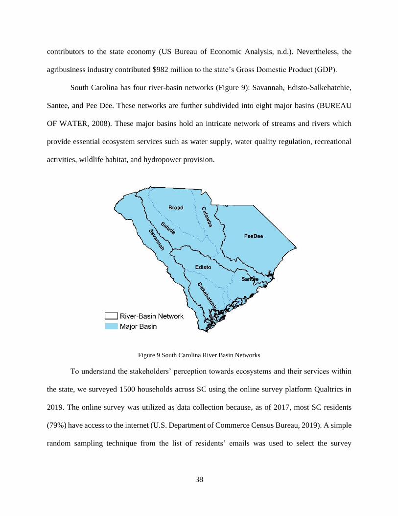
38
contributors to the state economy (US Bureau of Economic Analysis, n.d.). Nevertheless, the
agribusiness industry contributed $982 million to the state’s Gross Domestic Product (GDP).
South Carolina has four river-basin networks (Figure 9): Savannah, Edisto-Salkehatchie,
Santee, and Pee Dee. These networks are further subdivided into eight major basins (BUREAU
OF WATER, 2008). These major basins hold an intricate network of streams and rivers which
provide essential ecosystem services such as water supply, water quality regulation, recreational
activities, wildlife habitat, and hydropower provision.
Figure 9 South Carolina River Basin Networks
To understand the stakeholders’ perception towards ecosystems and their services within
the state, we surveyed 1500 households across SC using the online survey platform Qualtrics in
2019. The online survey was utilized as data collection because, as of 2017, most SC residents
(79%) have access to the internet (U.S. Department of Commerce Census Bureau, 2019). A simple
random sampling technique from the list of residents’ emails was used to select the survey

39
respondents. To ensure representation from different counties, the number of samples taken was
considered in proportion to the county population.
Furthermore, to consider the household's geographic location, the zip codes provided by
the respondents were used to calculate the centroid of the zip code area through ArcGIS. This
became a representation of the respondents’ household location. The geographic location was used
to correlate the respondents’ characteristics and the proximity of their household to nearby
environmental attributes such as stream quality and the presence of protected areas.
Survey design
The survey instrument consisted of four sections. Section 1 elicited baseline information
about the respondents’ understanding of the concepts of ecosystem and ecosystem services. This
section also elicited the respondents’ satisfaction rating towards the current state of the ecosystem
within their vicinities, such as the general impression of the streams and households’ water quality,
the quality of air, the amount of water that they can access, and the overall impression to the quality
of the environment in the area. The second section was an infographic of the terminologies and
concepts that were used throughout the survey. This ensures that respondents have a similar
understanding of the research questions. Section 3 elicits their preference to priority ecosystem
and ecosystem services. Provided with a list, respondents were asked to rank the listed ecosystem
and ecosystem services, according to their prioritization, highlighting that funds for conservation
programs are limited. The last section included questions about demographic characteristics.
The survey instrument was pre-tested with 32 residents of SC. The pre-testing evaluated
the initial knowledge and perception of the respondents towards ecosystem services and
conservation programs. Also, the pre-testing provided final inputs to the list of the commonly
known ecosystem and ecosystem services in the area resulting in a more robust questionnaire

40
specifically designed for South Carolina residents. Lastly, the pre-testing evaluated the wording,
timing, etc., of the survey instrument.
The survey instrument was reviewed and approved by the Clemson University Institutional
Review Board (IRB) to ensure that ethical guidelines on research activities involving human
subjects are followed. The IRB approval number is IRB2018 – 139.
Analysis of ranked preference
Respondents were provided a list of ecosystems and ecosystem services as their options to
choose from. The list was based on a focus group discussion workshop conducted as part of the
study's preliminary activities. Each respondent was asked to rank the options according to their
preferred prioritization, considering a limited implementation budget for conservation programs
to improve or enhance these services. This method was also done for different ecosystems to elicit
the priority ecosystems according to respondents' preferences (Table 4).
Table 4 List of ecosystems and ecosystem services for ranking
List of Ecosystems List of Ecosystem Services
• forests • water quality (water quality regulation)
• rivers/lakes • water supply (abundance of accessible water)
• farm/agricultural land • air quality (air quality regulation such as carbon
sequestration, filtering air pollution)
• wetland/marshes • wildlife and habitat conservation
• mountain • tourism and recreation (such as biking, walking, trail
hiking)
• coastal plains/beaches • heritage and cultural site importance
• ecosystems with
recreational function • hunting activities
• fishing activities
Henry Garrett’s ranking technique was utilized to analyze the overall ranked preference.
Garrett’s ranking technique is used primarily to determine the collective rank of options using a
score value (Arunkaumar et al., 2018; Dhanavandan, 2016; Sedaghat, 2011). The ranking
technique begins with estimating the percent position score of the options using the equation:
41
Percent positioni = 100 (𝑅𝑖𝑗−0.5)
𝑁𝑗 (1)
Where:
Rij = Rank given for the ith option by the jth respondent
Nj = Number of variables ranked by the jth respondent
The percent position estimated is converted through Garrett’s table (Appendix C) to
determine the total rank score of the ith option. The rank scores for each option i are added to get
the overall value of scores. Eventually, the mean value of scores is calculated by dividing the
overall rank scores by the number of respondents. The mean value of scores is ranked highest to
lowest to determine the hierarchy of options (Dhanavandan, 2016).
Equation (1) was used to all ranked attributes in the study – the rank of priority ecosystem
and the rank of priority ES. In this manner, the resulting order identifies the priority ecosystem
and ES of the respondents.
Understanding the respondents’ preference
A maximum likelihood regression analysis was used to examine the respondents'
characteristics that could have a statistically significant effect on their top-ranked options.
Furthermore, the regression analysis provides information on which among the options will
respondents likely select based on their differing characteristics. Since the nature of the dependent
variable is categorical, the likelihood model that was used is a Multinomial Logistic regression or
Multi-Logit regression (Greene, 1980).
The Multi-Logit regression is a non-linear regression that deals with multiple categorical
situations. The model assumes that the options presented to a decision-maker are mutually
exclusive, hence not correlated with each other. The model estimates the likelihood of choosing
one option over other options. Because the options among the ecosystems and ecosystem services

42
are unordered, the Multi-Logit model analyzes the primary question of “What is the respondent’s
priority ecosystem and ES among the list of options?”. The Multi-Logit regression analyzes if a
specific option is “more or less preferred” in comparison to another option. The equation of the
regression is as follows:
Pij = 𝒆
∑ 𝜶+ 𝜷𝒌𝒋𝑿𝒌𝒋𝒊𝑲𝒋=𝟏
∑ 𝒆∑ 𝜶+ 𝜷𝒌𝒋𝑿𝒌𝒋𝒊
𝑲𝒋=𝟏𝑲
𝒋=𝟏
(2)
Where Pij is the estimated likelihood of choosing the option j for respondent i, or in the
case of the study, the priority ecosystem or ES of respondent i. Furthermore, the numerator and
the denominator depict the odds ratio of the chosen option in comparison to others. With α as a
constant coefficient while βkj is a vector of coefficients corresponding to the vector of attributes
Xkji. Attribute X could be any characteristic or attributes that have a significant contribution to the
respondent’s decision. The list of attributes used in the models is summarized in Table 5.
Table 5 Summary of attributes in the Multi-Logit model
Attribute Description Levels
Endogenous variables
• Priority
ecosystem
the ecosystem which respondent
ranked as 1st priority in the ranking
analysis
1 - forest; 2 - rivers/lakes; 3 -
farm/agricultural land; 4 -
others
• Priority
ecosystem service
the ecosystem service which
respondent ranked as 1st priority in
the ranking analysis
1 - water quality; 2 - water
supply; 3 - other ES
Exogenous variables
• Satisfaction
rating to the
overall quality of
water
5-point Likert scale response to the
perceived satisfaction towards the
current water quality in the area,
reclassified into two levels
1 - satisfied; 0 - otherwise
• Satisfaction
rating to the
abundance or
amount of water
accessible to the
household
5-point Likert scale response to the
perceived satisfaction towards the
current water quality in the area,
reclassified into two levels
1 - satisfied; 0 - otherwise
• Satisfaction
rating to the
5-point Likert scale response to the
perceived satisfaction towards the 1 - satisfied; 0 - otherwise

43
overall state of
the environment
in the area
current water quality in the area,
reclassified into two levels
• Age age of the respondent year
• Income bracket overall income category of the
household
1 - less than $10,000 -
$49,999; 2 - $50,000 -
$99,999; 3 - more than
$100,000
• Distance to an
impaired stream
the proximity of the zip code centroid
to the nearest impaired stream meters
• Distance to a
good water body
the proximity of the zip code centroid
to the nearest good water body meters
• Distance to a
protected area
the proximity of the zip code centroid
to the nearest protected area meters
• Respondents’
residential region
Geographic region of the
respondents’ residence
1 – Lowcountry/coastal; 2 –
midland; 3 - upstate
The satisfaction rating and preferences towards an ecosystem or ecosystem service were
included in the exogenous variables. To simplify the categories as inputs to the regression model,
the satisfaction rating was consolidated and reclassified into a dummy variable, taking a value of
1 (satisfied) or 0 (otherwise). Respondents who answered 4 or 5 in their satisfaction rating was
reclassified into 1, while the other ratings were classified into 0.
Following previous studies linking the demographic factors and its influence on
environmental values and preferences (Abdul-Wahab & Abdo, 2010; Leviston et al., 2018;
Mangiafico, Obropta, & Rossi-Griffin, 2012; Olander et al., 2018), demographic variables are
included in the model. Furthermore, socio-economic characteristics are typical factors used in
evaluating decision-making as this constitutes constraint attributes to respondents. This is typical
to valuation and stakeholder involvement studies (Mangiafico et al., 2012; Marsh, 2014; Seriño et
al., 2017; Small, Munday, & Durance, 2017; Soley et al., 2019; J.C.P. Ureta et al., 2016).
Proximity to monitored ecosystems was included to represent a possible distance-effect of
the quality of these ecosystems to the preference of the respondents. Monitored ecosystems are

44
ecosystems that are regularly monitored and managed by authorities or landowners as indicators
for environmental health. For this study, we focused on impaired streams - streams that did not
meet the water quality standards and at least not open for public access due to water quality issues;
water bodies such as lakes, large rivers, and ponds that are evaluated as with good quality
(BUREAU OF WATER, 2008, 2011; South Carolina Department of Health and Environmental
Control, 2018); and protected areas - public and privately protected lands which were classified
by US Geological Survey (USGS) through the Protected Area Database of the United States (PAD-
US) (US Geological Survey (USGS) Gap Analysis Project (GAP), 2012) and a privately monitored
dataset of The Nature Conservancy (TNC) (personal communication, 2019) in South Carolina.
The proximity from monitored ecosystems could affect the respondent’s preference since areas
that could provide prime ecosystem services may not be equally distributed across the landscape
(Lin et al., 2019; Watts et al., 2017). The proximities affect the stakeholders’ preference as
feedback of the impression of the quality of the nearby ecosystem (Weaver & Lawton, 2008),
while the quality of the ecosystems can be associated with possible interventions.
Assessing the satisfaction rating of respondents
The respondents’ impression of the general state of their environment was also elicited
using a 5-point Likert scale satisfaction rating (1 being the lowest and 5 being the highest). Survey
participants were asked four general questions about aspects of the environment: (1) satisfaction
with the overall quality of water, (2) satisfaction with the abundance or amount of water accessible
to their household, (3) satisfaction with the quality of air within their area, and (4) satisfaction with
the overall state of the environment in their area. This question could serve as a feedback
mechanism for conservation managers and professionals to understand how residents perceive the
current state of the ecosystem and ecosystem services. This could indicate their awareness on the
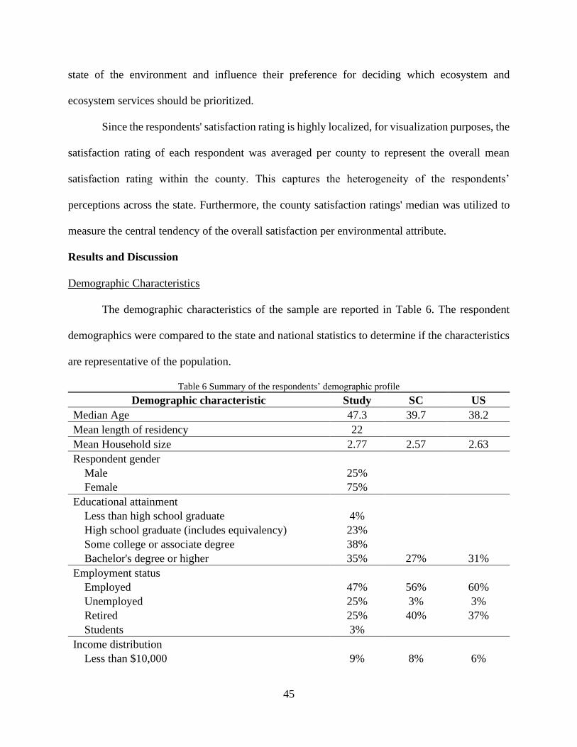
45
state of the environment and influence their preference for deciding which ecosystem and
ecosystem services should be prioritized.
Since the respondents' satisfaction rating is highly localized, for visualization purposes, the
satisfaction rating of each respondent was averaged per county to represent the overall mean
satisfaction rating within the county. This captures the heterogeneity of the respondents’
perceptions across the state. Furthermore, the county satisfaction ratings' median was utilized to
measure the central tendency of the overall satisfaction per environmental attribute.
Results and Discussion
Demographic Characteristics
The demographic characteristics of the sample are reported in Table 6. The respondent
demographics were compared to the state and national statistics to determine if the characteristics
are representative of the population.
Table 6 Summary of the respondents’ demographic profile
Demographic characteristic Study SC US
Median Age 47.3 39.7 38.2 Mean length of residency 22
Mean Household size 2.77 2.57 2.63 Respondent gender
Male 25%
Female 75%
Educational attainment
Less than high school graduate 4%
High school graduate (includes equivalency) 23%
Some college or associate degree 38%
Bachelor's degree or higher 35% 27% 31%
Employment status
Employed 47% 56% 60%
Unemployed 25% 3% 3%
Retired 25% 40% 37%
Students 3%
Income distribution
Less than $10,000 9% 8% 6%

46
10k to 50k 44% 40% 35%
50k to 100k 33% 31% 30%
100k to 150k 11% 12% 15%
more than 150k 5% 9% 14%
Source: (United States Census Bureau, 2019c)
Results show that, in terms of educational attainment, most of the respondents have some
college degree. Furthermore, the number of respondents with a bachelor’s degree or higher
resembles the statistics of the state and national population. In terms of annual household income,
the sampling distribution is closely similar to the state and national household income distribution.
Overall, the results of the demographic characteristics indicate that the sampled respondents
represent the demographic characteristics of the population.
The high frequency of unemployed respondents is not uncommon in online surveys since
they can use online surveys as an extra income source (Ford, 2017; S. M. Smith, Roster, Golden,
& Albaum, 2016). Furthermore, the gender imbalance of respondents is a common occurrence
particularly in survey-based studies, since female household decision-makers tend to stay and
manages the household (Calderon et al., 2012; J.C.P. Ureta et al., 2016; Julie Carl P. Ureta, Lasco,
Sajise, & Calderon, 2014). Moreover, studies showed that the participation rate of female
respondents is higher for mail-in and online platforms due to the differences of female and male
values operating in a gendered online environment (Mulder & de Bruijne, 2019; W. G. Smith,
2008).
Residents’ impression of the current state of the environment
The results of the satisfaction ratings are reported in Table 7 (see Appendix D, E, F, G).
Results showed that survey participants have the highest satisfaction rating in water supply
characteristic followed by the air quality, while the water quality characteristic and the overall
quality of the environment yielded the lowest rating with a mean rating that is not significantly
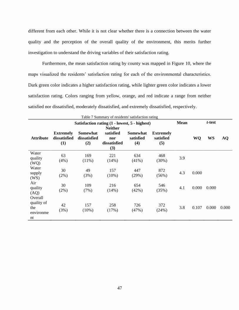
47
different from each other. While it is not clear whether there is a connection between the water
quality and the perception of the overall quality of the environment, this merits further
investigation to understand the driving variables of their satisfaction rating.
Furthermore, the mean satisfaction rating by county was mapped in Figure 10, where the
maps visualized the residents’ satisfaction rating for each of the environmental characteristics.
Dark green color indicates a higher satisfaction rating, while lighter green color indicates a lower
satisfaction rating. Colors ranging from yellow, orange, and red indicate a range from neither
satisfied nor dissatisfied, moderately dissatisfied, and extremely dissatisfied, respectively.
Table 7 Summary of residents' satisfaction rating
Satisfaction rating (1 - lowest, 5 - highest) Mean t-test
Attribute
Extremely
dissatisfied
(1)
Somewhat
dissatisfied
(2)
Neither
satisfied
nor
dissatisfied
(3)
Somewhat
satisfied
(4)
Extremely
satisfied
(5)
WQ WS AQ
Water
quality
(WQ)
63
(4%)
169
(11%)
221
(14%)
634
(41%)
468
(30%) 3.9
Water
supply
(WS)
30
(2%)
49
(3%)
157
(10%)
447
(29%)
872
(56%) 4.3 0.000
Air
quality
(AQ)
30
(2%)
109
(7%)
216
(14%)
654
(42%)
546
(35%) 4.1 0.000 0.000
Overall
quality of
the
environme
nt
42
(3%)
157
(10%)
258
(17%)
726
(47%)
372
(24%) 3.8 0.107 0.000 0.000
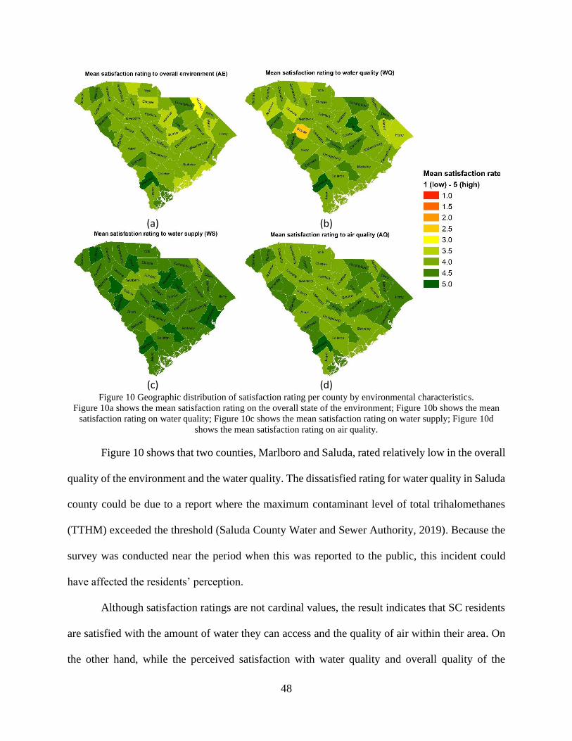
48
(a)
(b)
(c)
(d)
Figure 10 Geographic distribution of satisfaction rating per county by environmental characteristics.
Figure 10a shows the mean satisfaction rating on the overall state of the environment; Figure 10b shows the mean
satisfaction rating on water quality; Figure 10c shows the mean satisfaction rating on water supply; Figure 10d
shows the mean satisfaction rating on air quality.
Figure 10 shows that two counties, Marlboro and Saluda, rated relatively low in the overall
quality of the environment and the water quality. The dissatisfied rating for water quality in Saluda
county could be due to a report where the maximum contaminant level of total trihalomethanes
(TTHM) exceeded the threshold (Saluda County Water and Sewer Authority, 2019). Because the
survey was conducted near the period when this was reported to the public, this incident could
have affected the residents’ perception.
Although satisfaction ratings are not cardinal values, the result indicates that SC residents
are satisfied with the amount of water they can access and the quality of air within their area. On
the other hand, while the perceived satisfaction with water quality and overall quality of the
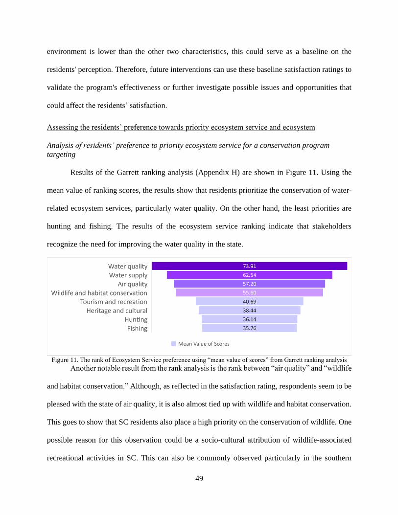
49
environment is lower than the other two characteristics, this could serve as a baseline on the
residents' perception. Therefore, future interventions can use these baseline satisfaction ratings to
validate the program's effectiveness or further investigate possible issues and opportunities that
could affect the residents’ satisfaction.
Assessing the residents’ preference towards priority ecosystem service and ecosystem
Analysis of residents’ preference to priority ecosystem service for a conservation program
targeting
Results of the Garrett ranking analysis (Appendix H) are shown in Figure 11. Using the
mean value of ranking scores, the results show that residents prioritize the conservation of water-
related ecosystem services, particularly water quality. On the other hand, the least priorities are
hunting and fishing. The results of the ecosystem service ranking indicate that stakeholders
recognize the need for improving the water quality in the state.
Figure 11. The rank of Ecosystem Service preference using “mean value of scores” from Garrett ranking analysis
Another notable result from the rank analysis is the rank between “air quality” and “wildlife
and habitat conservation.” Although, as reflected in the satisfaction rating, respondents seem to be
pleased with the state of air quality, it is also almost tied up with wildlife and habitat conservation.
This goes to show that SC residents also place a high priority on the conservation of wildlife. One
possible reason for this observation could be a socio-cultural attribution of wildlife-associated
recreational activities in SC. This can also be commonly observed particularly in the southern

50
region of the United States. Since wildlife-associated recreation generates economic benefits for
the state of SC (Willis & Straka, 2016), this plays an important influence on the prioritization
preference of the residents.
Since the rank analysis identified water quality as the priority ecosystem service, we
analyzed the possible factors which lead to this preference. Using the Multi-Logit model, we
compared respondents' likelihood to choose water quality over water supply and other “non-water
related” ES.
Table 8 Multi-Logit regression5 of resident’s priority ecosystem service
Predictor
vs. Water Supply vs. other ES
Coef
(SE)
Relative
risk
ratio
Coef
(SE)
Relative
risk
ratio
Intercept -1.882***
(0.40)
0.15 -0.502^
(0.28)
0.61
Satisfaction rating to water quality (satisfied) 0.620*
(0.24)
1.86 0.326*
(0.16)
1.38
Satisfaction rating to water supply (satisfied) -0.908***
(0.27)
0.40 -0.034
(0.20)
0.97
Satisfaction rating to overall environmental quality
(satisfied)
0.002
(0.22)
1.00 -0.117
(0.15)
0.89
Age 0.003
(0.01)
1.00 -0.014***
(0.00)
0.99
Income $50,000 - $99,999 0.182
(0.20)
1.20 -0.206^
(0.14)
0.81
Income more than $100,000 -0.082
(0.26)
0.92 -1.013***
(0.22)
0.36
Distance to an impaired stream -0.003
(0.07)
1.00 0.170**
(0.05)
1.18
Distance to a good water body 0.053
(0.09)
1.05 0.015
(0.06)
1.02
Residents from the midland region -0.086
(0.22)
0.92 0.107
(0.15)
1.11
Residents from the upstate region 0.222
(0.23)
1.25 0.319^
(0.16)
1.38
5 The Multi-Logit regression coefficient shows the log-odds ratio while the relative risk ratio is the probability
associated to the likelihood of the respondent’s choice considering the independent variable as the respondent’s
characteristic. A value of 1 means that there is no change, hence the respondents are indifferent between the
alternative and the baseline. A RR ratio greater than 1 represents that respondents have higher likelihood to choose
the alternative compared to the baseline.
The Multi-Logit regression model was ran in the R Studio software using the “mlogit” package.

51
Likelihood ratio test : chisq = 77.603 (p.value = 9.9815e-09) McFadden R^2: 0.03
*** pval < 0.001 ** pval < 0.01
* pval < 0.05
^ pval < 0.10
The model evaluated the respondents’ likely choice of priority ecosystem service between
the baseline priority ES - water quality - and two other alternatives: water supply and other ES.
Table 8 shows the result of the multinomial logit regression displaying the factors affecting the
respondent’s preference and the probability of the respondent to choose between the baseline as
compared to the alternative.
Likelihood of choosing water quality vs. water supply as the preferred priority ecosystem service
Results in Table 8 show that the satisfaction ratings towards water quality and water supply
are likely to affect residents' preference. Notably, residents who are satisfied with their current
water quality are 86% more likely to prioritize water supply. On the other hand, residents who are
satisfied with their water supply are 60% more likely to prioritize water quality as the target for
conservation programs. This shows that residents’ prioritization towards water quality regulation
as ES, although more preferred by respondents, does not mean that water supply should not be
prioritized at all. Water quality regulation and water supply provision, although different
ecosystem services, are usually dealt with and managed together (Bai, Ochuodho, & Yang, 2019;
Cosgrove & Loucks, 2015; Vigerstol & Aukema, 2011).
Likelihood of choosing water quality vs. other non-water related ES as preferred priority
ecosystem service
Comparing the resident’s preference between water quality and other ES showed more
variables affecting their choices, namely: satisfaction rating to water quality, socio-economic
factors such as age and income, proximity to the nearest impaired stream, and if residents’
household is located in the upstate region.
52
Similar to the water supply, respondents that are satisfied with the quality of water are 38%
more likely to prioritize other ES. This could imply that only when respondents are satisfied with
water quality will they be more likely to prioritize other ES. This follows the results of previous
studies showing that residents prioritize the improvement of water quality (Aguilar et al., 2018;
Brox et al., 1996; Calderon et al., 2012; Castro et al., 2016; Doherty et al., 2014; Khan et al., 2019;
Khan & Zhao, 2019).
Meanwhile, socio-economic covariates suggest that older respondents have a higher
likelihood to prioritize water quality. Particularly, as respondents increase their age by a year, the
likelihood that they will choose water quality as compared to other ES increases by 1%. This could
possibly be associated with house ownership. Older respondents are typically homeowners (70%
of the respondents), where access to adequate water quality is an essential component in owning a
house in a specific area.
Furthermore, in terms of income levels, results show that households with higher income
levels are more likely to prioritize water quality than other ES. Particularly, households with an
annual income of $50,000 to $99,999 are 19% more likely to prioritize water quality as compared
to households with income lower than $50,000. Moreover, households with an annual income of
more than $100,000 are 64% more likely to prioritize water quality as compared to households
with income lower than $50,000. This could be associated with the cost of accessing a good quality
of water. In recent years, households install filtration systems or simply buy bottled water to ensure
high water quality for consumption (Quick, 2018). Households with income higher than the state’s
mean household income of $72,000 (SC Department of Employment and Workforce, 2018; United
States Census Bureau, 2018) implies more capable of installing filtration systems while the other
less expensive alternative is to buy bottled water. Therefore, an improvement in the water quality

53
could decrease these costs for households. In any case, the income variable showed that water
quality is more likely to be prioritized by residents as compared to other non-water related
ecosystem services.
In terms of the proximity to monitored ecosystems, only the distance to impaired streams
showed a statistically significant effect. In this case, a 1-kilometer increase in distance between
the respondent’s household from the nearest impaired stream implies that these respondents are
18% more likely to choose other ES to be prioritized rather than water quality. This could be
because respondents living farther from an impaired stream do not see or are not aware of an
impaired stream's negative impact. Hence, the likelihood of prioritizing water quality over other
ES also decreases.
Residents living in the upstate region are 38% more likely to prioritize other ES compared
to those in the Lowcountry or coastal areas. This could be attributed to the satisfaction rating of
the upstate residents to water quality. Overall, 87% of the respondents from the upstate gave a
satisfactory rating to the water quality, while 85% for the Lowcountry. Since more residents in the
upstate are satisfied with the water quality, this could be the reason why they are more likely to
choose other ES as compared to Lowcountry/coastal residents.
Overall, the result for the intercepts in both comparisons showed to be statistically
significant favoring water quality. This indicates that suppose all other factors are constant,
respondents are more likely to prioritize water quality than water supply or other ES.
Analysis of residents’ preference to priority ecosystem for conservation program intervention
As with the ecosystem service preference analysis, we analyzed respondents' preference
towards prioritization of the ecosystem. Similarly, understanding these preferences towards
priority ecosystems can narrow the appropriate conservation program recommendation for
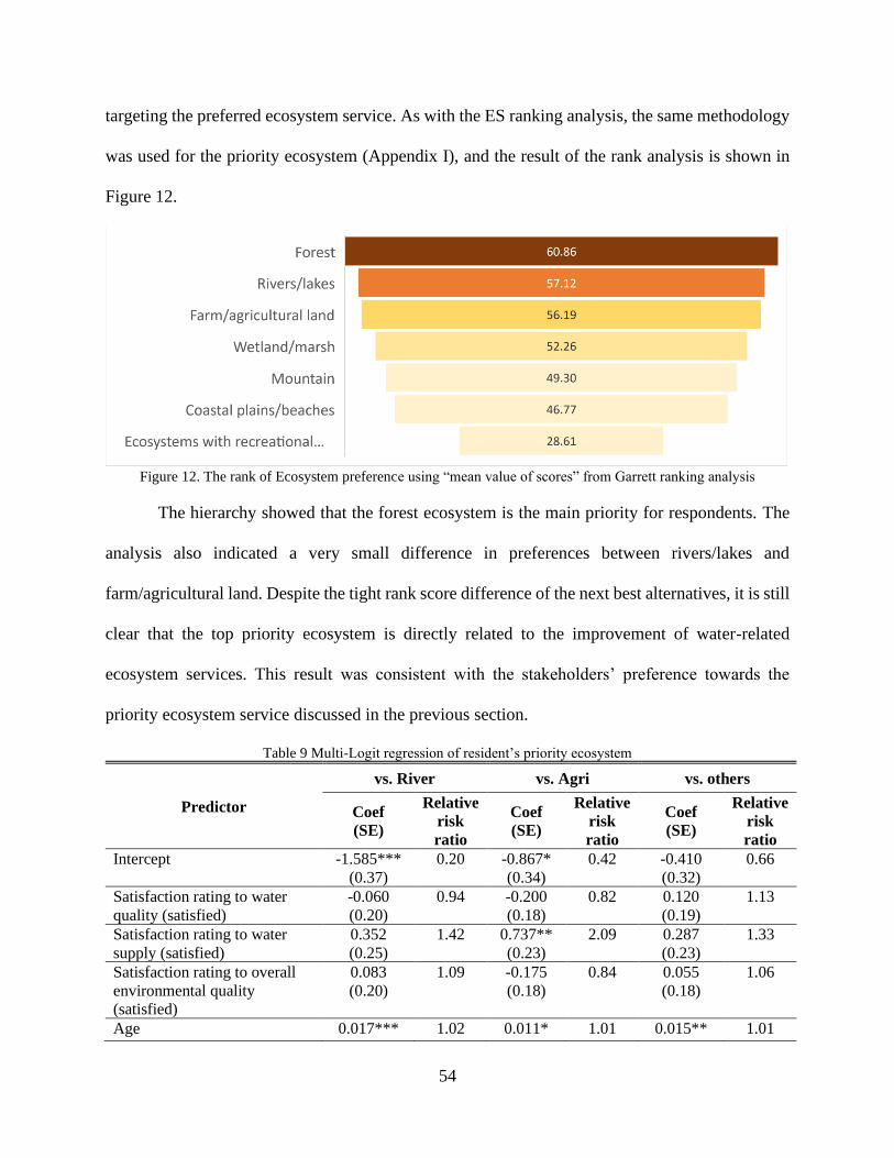
54
targeting the preferred ecosystem service. As with the ES ranking analysis, the same methodology
was used for the priority ecosystem (Appendix I), and the result of the rank analysis is shown in
Figure 12.
Figure 12. The rank of Ecosystem preference using “mean value of scores” from Garrett ranking analysis
The hierarchy showed that the forest ecosystem is the main priority for respondents. The
analysis also indicated a very small difference in preferences between rivers/lakes and
farm/agricultural land. Despite the tight rank score difference of the next best alternatives, it is still
clear that the top priority ecosystem is directly related to the improvement of water-related
ecosystem services. This result was consistent with the stakeholders’ preference towards the
priority ecosystem service discussed in the previous section.
Table 9 Multi-Logit regression of resident’s priority ecosystem
Predictor
vs. River vs. Agri vs. others
Coef
(SE)
Relative
risk
ratio
Coef
(SE)
Relative
risk
ratio
Coef
(SE)
Relative
risk
ratio
Intercept -1.585***
(0.37)
0.20 -0.867*
(0.34)
0.42 -0.410
(0.32)
0.66
Satisfaction rating to water
quality (satisfied)
-0.060
(0.20)
0.94 -0.200
(0.18)
0.82 0.120
(0.19)
1.13
Satisfaction rating to water
supply (satisfied)
0.352
(0.25)
1.42 0.737**
(0.23)
2.09 0.287
(0.23)
1.33
Satisfaction rating to overall
environmental quality
(satisfied)
0.083
(0.20)
1.09 -0.175
(0.18)
0.84 0.055
(0.18)
1.06
Age 0.017*** 1.02 0.011* 1.01 0.015** 1.01
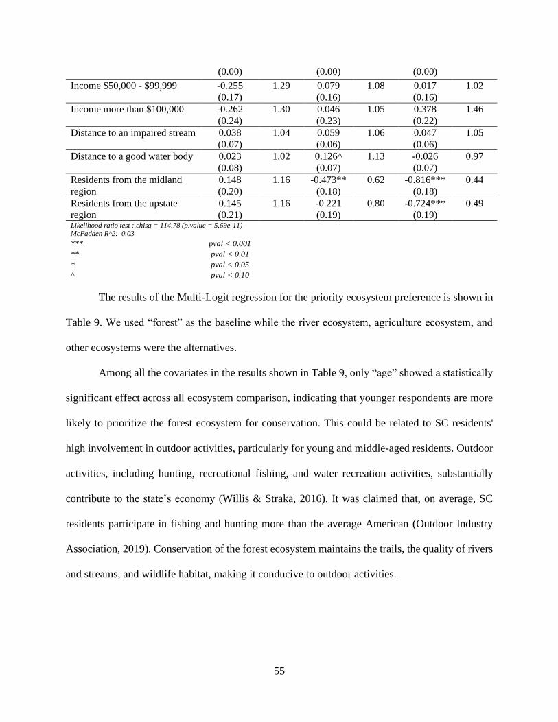
55
(0.00) (0.00) (0.00)
Income $50,000 - $99,999 -0.255
(0.17)
1.29 0.079
(0.16)
1.08 0.017
(0.16)
1.02
Income more than $100,000 -0.262
(0.24)
1.30 0.046
(0.23)
1.05 0.378
(0.22)
1.46
Distance to an impaired stream 0.038
(0.07)
1.04 0.059
(0.06)
1.06 0.047
(0.06)
1.05
Distance to a good water body 0.023
(0.08)
1.02 0.126^
(0.07)
1.13 -0.026
(0.07)
0.97
Residents from the midland
region
0.148
(0.20)
1.16 -0.473**
(0.18)
0.62 -0.816***
(0.18)
0.44
Residents from the upstate
region
0.145
(0.21)
1.16 -0.221
(0.19)
0.80 -0.724***
(0.19)
0.49
Likelihood ratio test : chisq = 114.78 (p.value = 5.69e-11) McFadden R^2: 0.03 *** pval < 0.001
** pval < 0.01
* pval < 0.05
^ pval < 0.10
The results of the Multi-Logit regression for the priority ecosystem preference is shown in
Table 9. We used “forest” as the baseline while the river ecosystem, agriculture ecosystem, and
other ecosystems were the alternatives.
Among all the covariates in the results shown in Table 9, only “age” showed a statistically
significant effect across all ecosystem comparison, indicating that younger respondents are more
likely to prioritize the forest ecosystem for conservation. This could be related to SC residents'
high involvement in outdoor activities, particularly for young and middle-aged residents. Outdoor
activities, including hunting, recreational fishing, and water recreation activities, substantially
contribute to the state’s economy (Willis & Straka, 2016). It was claimed that, on average, SC
residents participate in fishing and hunting more than the average American (Outdoor Industry
Association, 2019). Conservation of the forest ecosystem maintains the trails, the quality of rivers
and streams, and wildlife habitat, making it conducive to outdoor activities.
56
Likelihood of choosing forest ecosystem vs. river ecosystem as the preferred priority ecosystem
Results presented in Table 9 show that apart from the respondent's age and the intercept,
non among the other variables that we have investigated showed statistically significant evidence
that residents prioritize the forest ecosystem compared to the river ecosystem. However, the
intercept indicates that, if all variables are held constant, residents are 80% more likely to prioritize
forest ecosystems for conservation programs as compared to the river ecosystem.
Likelihood of choosing forest ecosystem vs. agricultural ecosystem as the preferred priority
ecosystem
Since one of the major beneficiaries of ecosystem services is agriculture, we also compared
the respondents’ prioritization between forest ecosystems and agroecosystems. Agriculture is also
the third-ranked priority ecosystem in the earlier rank analysis in Figure 12.
Results in Table 9 show that respondents who are primarily satisfied with the current water
supply are 109% more likely to choose the agriculture ecosystem than the forest ecosystem to be
prioritized. Residents’ perception of the abundance of water in SC could be why they choose
agriculture activities. Residents may believe there is enough water for crop production in the state.
In terms of the distance to monitored ecosystems, results in Table 9 showed that as the
distance of the center of the household’s zip code goes farther from a good water body, the
respondent is more likely to choose the agroecosystem the priority ecosystem to be conserved by
13%. This result could be attributed to SC residents preferring agricultural land to forest land.
Mainly if they are located in an agriculturally dominated area or agriculture is a significant income
source in their household, such as in the midland region of SC. South Carolina has historically
been dependent on natural resources, including agriculture, for its economic growth (Willis &
Straka, 2016). However, while urbanization and industrial areas continue to develop, the
agriculture industry continues to decline. In fact, the GDP contribution from farms in 1997 only
57
amounts to 0.76% and continues to decline, amounting to 0.30% in 2017 (US Bureau of Economic
Analysis, n.d.). However, around 14% of the land is still classified as agricultural (US Geological
Survey (USGS) Gap Analysis Project (GAP), 2012); hence, this shows that a substantial amount
of households are heavily dependent on agriculture. Respondents under these conditions tend to
prioritize the improvement of the agroecosystem rather than the forest ecosystem.
On the other hand, respondents residing in the midland region are 38% more likely to
prioritize the forest ecosystem as compared to those who reside in the Lowcountry. The midland
region showed a low satisfaction rating for water quality relative to the other regions (Figure 10b).
Therefore, since enhanced forest management is attributed to an improvement in water quality
(Aguilar et al., 2018), the urgency from the residents’ satisfaction rating likely contributes to their
preference for prioritizing the forest ecosystem for conservation.
Lastly, the intercept also shows that holding all other factors as constant, residents are more
likely to prioritize forest ecosystems by 58% as compared to the agriculture ecosystem.
Likelihood of choosing forest ecosystem vs. “other ecosystems” as preferred priority ecosystem
In comparison to “other ecosystems,” results in Table 9 revealed that the residents'
geographic region indicates statistically significant evidence that it affects the respondents'
preference.
Residents from both midland and the upstate are 51% to 56% more likely to choose the
forest ecosystem for conservation as compared to residents from the Lowcountry. While the
midland residents' preference could be attributed to their satisfaction rating to water quality, the
upstate’s preference could be attributed to the land cover. Since the topography of the upstate is
hilly and mountainous, the majority of the land cover classified as forested area are in this region
(US Geological Survey (USGS) Gap Analysis Project (GAP), 2012). Therefore, upstate residents
58
have better familiarity with the ecosystem and ecosystem services of the forest which benefits
them. Hence, they choose to prioritize the forest ecosystem.
Overall, the results reinforce the rank analysis in which the residents of SC prefer to
prioritize forest ecosystems for conservation compared to other ecosystems. Essentially,
respondents to our survey revere to prioritize the forest ecosystem because they are aware that it
is the main source of the primary ecosystem services in SC which directly benefits them.
Summary and Conclusion
This study examined the priorities for conservation of ecosystems and ecosystem services
for residents in South Carolina, USA. Since residents are typically the final recipients of ecosystem
services, identification of priority ecosystem and ecosystem services from the public’s outlook
could help in the strategic implementation of conservation programs. Nevertheless, to the best of
our knowledge, no study has previously investigated SC residents' preference regarding ES.
Results showed that SC residents are likely to prioritize water-related ecosystem services,
particularly the improvement to water quality regulation, while their least priorities are fishing and
hunting. Although South Carolina residents are actively involved in fishing, hunting, and outdoor
activities, water quality improvement still poses to be their top priority since water quality
improvement also benefits other ecosystem services, including fishing and other outdoor activities.
Similarly, this was also reflected in the respondents' mean satisfaction rating through their general
impression of the current state of the environment in SC. The satisfaction rating to the water quality
and the impression of the overall quality of the environment scored lowest as compared to water
supply and air quality. While further investigation is still needed to determine the specific reason
why this is the case, the results of this study could be used as a baseline for monitoring these
characteristics.
59
Furthermore, these results are consistent with the residents’ preference to prioritize water
quality regulation as the primary ecosystem service for conservation program targeting. However,
their preferences towards water quality improvement do not discredit the importance of
maintaining the continuous water supply provision, as was evident in the maximum likelihood
analysis. Most covariates did not yield statistically significant evidence when comparing water
quality and water supply as the priority ecosystem service. Therefore, as state resource managers
continually update their water plans, including monitoring systems for water quality improvement
would ensure that they address the challenge of meeting the water demand while also meeting the
public’s satisfaction standards for water quality.
In terms of ecosystem preference, respondents to our survey indicated that the forest
ecosystem is the priority ecosystem to be conserved. The reasons for this preference also align
with their ecosystem service preference. Respondents are aware of the forest ecosystem's direct
linkage to water-related ecosystem services; therefore, they opt to choose to conserve the
ecosystem that also enhances their primary priority ecosystem service. Thus, in planning for
conservation interventions, prioritizing the conservation programs for the forested land would reap
more support and possible participation from the public.
The prioritization ranking of SC residents also revealed their preferences towards the
primary ecosystem and ecosystem service for conservation. Apart from the satisfaction ratings,
socio-economic factors such as age and income also showed statistical evidence that affects the
respondents’ prioritization. Also, proximities to monitored ecosystems revealed to have a
significant contribution in evaluating respondents’ preferences. The regression result using the
proximity of monitored ecosystems also showed that the quality of these ecosystems affects the
residents’ perception and prioritization criteria. For instance, residents who live farther from an

60
impaired stream do not see the urgency of an improved water body hence will prioritize other
ecosystem services more than water quality regulation.
On the other hand, those who live in agriculture-dependent areas and near a good water
body will prioritize agriculture ecosystem rather than forest ecosystems because of the availability
of water that could be used for irrigation purposes. Furthermore, the geographic region of the
respondents showed a statistically significant contribution affecting their preference. Since
geographic regions have different landscape characteristics such as topography and land cover,
this could also affect the residents’ preference for conservation. Therefore, the results showed that
perception and impressions of nearby ecosystems and their geographic location affect their
preferences and prioritization. This analysis could be important in targeting the stakeholders that
could be involved in supporting the conservation programs. For instance, since younger residents
and residents with higher income are keen on forest conservation, designing sustainable financing
mechanisms or user-fee mechanisms could be tailor-fitted to this group. Knowing the residents’
priority ecosystem and ecosystem service for conservation is an essential initial step for conducting
a WTP study for conservation planning activities and as an economic basis for developing
sustainable financing mechanisms that will support conservation programs.
The use of SC residents’ perception, including satisfaction rating, to measure the public's
general impression towards the environment served as a feedback mechanism. Ensuring that the
public’s satisfaction standards are met translates into public support, hence could increase the
potential funding support for conservation programs. Understanding the results from their
perception can draw up insights for crafting strategic implementation of conservation programs
and further conservation studies. For instance, in 2013, in addressing the water supply problem,
the state tapped the residents’ ability to promote the efficient use of water through the
61
“WaterSense” program (US Environmental Protection Agency, 2013). The program encouraged
residents to install WaterSense labeled products to ensure that their households are using water-
saving technologies. The program was advertised and popularized by the “Every Drop Counts”
campaign of the state, which led to a savings of 677 million gallons of water annually (US
Environmental Protection Agency, 2013). This program proved that residents’ participation and
preferences could improve the implementation of conservation programs. Therefore, the results of
this study could provide important information on implementing conservation programs,
particularly in focusing on water quality and the forest ecosystem.
As the state water plans are continuously being updated by the state agencies and the South
Carolina Water Resources Center (SCWRC) to ensure that there is enough supply of water for
everyone, this study showed that there should also be a focus on the water quality regulation and
ecosystem conservation, particularly towards the forested land. Picking up from the results of this
study, further research endeavors focusing on water-related ecosystem services in SC could
provide better assessment and information about their conservation program priorities.
Furthermore, knowing the stakeholders' priority ecosystem and ecosystem services can be used for
designing specific valuation studies.
Since the study was focused on residents as the main stakeholder, further research will be
to look at other stakeholders’ perspectives such as farmers, landowners, tourists, and businesses,
which could provide more insights on the feasibility of implementing conservation programs.
Also, since the study was conducted on an online platform, the results of this study are limited to
inference regarding only residents with access to the internet. Although most residents across the
state have internet access, a substantial number of residents are still without online access.
Therefore, it is worth pursuing to examine the preferences of non-internet users on the matter.

62
Moreover, while the scale of the study focuses only on SC residents, it will be interesting for future
research to compare the residents’ preferences across different states or regions. This comparison
could provide a more comprehensive assessment of the decision-making factors that affect an
individual’s preference to prioritize an ecosystem or ecosystem service for conservation. Finally,
in pursuing sustainability as defined in the World Commission on Environment and Development
(WCED), future research and ES approaches should include a more diverse notion of social-
ecological systems by making it centered towards the stakeholder while not compromising the
ecosystem integrity. Therefore, future managers can draw insights from the results of this study to
craft strategic implementation of conservation programs by incorporating the residents' preference.

63
CHAPTER THREE
QUANTIFYING THE LANDSCAPE’S ECOLOGICAL BENEFITS: AN ANALYSIS OF THE
EFFECT OF LAND COVER CHANGE ON ECOSYSTEM SERVICES6
Introduction
Improvements in human well-being and landscape sustainability heavily depend on the
continuous provision of ecosystem services (ES). These services are direct and indirect benefits
that humans receive from ecosystems (Millenium Ecosystem Assessment, 2005). Different
ecosystems provide a wide array of ES, including supporting services (e.g., carbon cycle, nutrient
cycle, and water cycle), provisioning services (e.g., food, water, and raw materials), regulating
services (e.g., climate regulation, water filtration, and storm protection from forests and wetlands),
and socio-cultural services (e.g., traditions and nature-based recreational activities). However,
despite these multiple benefits, ecosystems are under constant threat of degradation, primarily
because of climate change and land-use change (Hoyer & Chang, 2014; Kindu, Schneider,
Teketay, & Knoke, 2016). For example, freshwater ecosystems are among the most affected and
extensively altered ecosystems on earth (Carpenter, Stanley, & Vander Zanden, 2011; Millenium
Ecosystem Assessment, 2005) as a result of increasing pressure from land conversion.
Land use change is a major driver of climate change across the world, but it can be managed
at a local or regional scale when ecosystem services are considered. However, land use-land cover
changes are often in conflict between two opposing models - economic expansion and ecological
conservation (Quintas-Soriano, Castro, Castro, & García-Llorente, 2016). Oftentimes, one is
favored over the other resulting in imbalanced resource management, causing a negative effect to
either aspect of development – economic or ecological. For example, agricultural and forest lands
near urban areas and industrialized complexes are prioritized for intense development for their
6 Chapter has been published in the Journal of Land. https://doi.org/10.3390/land10010021

64
high value for residential areas and urban expansion. This intensified development could result in
numerous ecological issues such as habitat fragmentation and biodiversity losses (Foley, 2005;
Lawler et al., 2014), changes in carbon balance and nutrient flows (Kreuter, Harris, Matlock, &
Lacey, 2001; Krkoška lorencová et al., 2016), landscape and water quality degradation (Hoyer &
Chang, 2014; Lautenbach, Kugel, Lausch, & Seppelt, 2011), and reduced protection from extreme
events (Murty et al., 2014; Seriño et al., 2017; Tõnisson et al., 2008). To balance economic
expansion and ecological conservation, the adoption of practices that focus on sustainable land
management (Abram et al., 2014; Quintas-Soriano et al., 2016) are important to provide both
economic and ecological benefits, aiding in climate change mitigation (Van Reeth, 2013; Wu,
2013).
The planting of cover crops in intensive agriculture systems is one example of sustainable
land management in the United States. Cover crops deliver significant benefits for soil and water
quality by providing soil cover when cash crops are not in season (Kaspar & Singer, 2011). There
are myriad ecological benefits that can be gained from implementation, including reduction in
nitrogen and topsoil leaching, increased water infiltration, and managing soil temperature
(Hoorman, Islam, Sundermeier, & Reeder, 2009). The reduction in topsoil loss and the use of
legumes that fix nitrogen often help reduce fertilizer inputs and reduce costs (Gabriel, Garrido, &
Quemada, 2013; Mase, Gramig, & Prokopy, 2017; Reeves, 1994). Furthermore, cover crops can
build soil organic matter; which is crucial to sustaining microbial activity and, ultimately, a
sustainable agriculture system (Fageria, 2012; Hobbs, 2007). Increasing soil health and decreasing
synthetic inputs can reduce the negative impact large scale agriculture has on water quality.
Combining no-till agriculture with cover crops may even yield more profit for farmers than
65
conventional agriculture systems (Pittelkow et al., 2015), and this type of operation closely mimics
natural systems and increases resilience (Hoorman et al., 2009).
Unfortunately, the perception that implementing cover crops can be a significant added
cost for many farmers has resulted in implementation among only around 5% of farmers in the
United States (Clay, Perkins, Motallebi, Plastina, & Farmaha, 2020; Dunn et al., 2016). Most of
the time, farmers do not know or understand how using these conservation practices can improve
productivity and monetary returns (Pittelkow et al., 2015). As climate change mitigation has
become more focused on agriculture systems, cover crops are being increasingly described as a
major part of climate change mitigation strategies, while land managers and extension specialists
are working to help increase cover crop usage (Arbuckle & Roesch-McNally, 2015). Therefore,
quantifying and analyzing changes on the landscape is an essential tool for information
dissemination and public awareness (S. Liu, Costanza, Troy, D’Aagostino, & Mates, 2010),
landscape and natural resource management (Costanza et al., 1997), policy-making and
optimization (Schägner, Brander, Maes, & Hartje, 2013), and incentives to implement
conservation programs strategically (Bateman et al., 2013; Kindu et al., 2016). With science and
technology continuously improving, new methodologies for quantifying and assessing land-use
change and its effects are becoming available.
Remote sensing and Geographic Information Systems (GIS) technology are commonly
used in data gathering and analysis of land use-land cover by classifying an area of the land and
mapping its distribution (Bai et al., 2019; Kindu et al., 2016; Wang, Lechner, & Baumgartl, 2018).
The availability of this technology has paved the way for quantifying ES using ES-based models.
One of the widely used ES-based models is the Integrated Valuation of Ecosystem Services and
Tradeoffs (InVEST). The InVEST is a suite of spatially explicit models for quantifying various
66
ES (Nelson et al., 2018; Sharps et al., 2017). The model can be applied over different spatial scales
depending on the resolution of the data inputs, making it flexible for post-processing of land use-
land cover (LULC) change analysis and ES tradeoff analyses. The main feature of the model is
that it uses biophysical equations for estimating an ES in a particular area within the landscape.
The model yields a map where pixels hold the ES information and can be used to identify the areas
with high ES provisions and show which land cover produces specific ES. Since InVEST has
readily available training materials, documentation, data repositories, and a support team, this
model has gained popularity and has been widely adopted for quantifying landscape ES-based
models (Sharps et al., 2017).
The Santee River Basin Network (SRBN) is a major river basin network in South Carolina
(SC) (Figure 13). It originates from the mountains in southern North Carolina and traverses the
upstate South Carolina to the coast (Hughes, Abrahamsen, Maluk, Reuber, & Wilhelm, 2000). The
majority of the SRBN’s land cover is classified as vegetated, with forest land covering 51% of the
landscape; wetland covers 12%, grassland 11%, shrubland and agriculture at 8%, water bodies at
4%, developed or urban areas covering at 14%, and barren land at less than 1% of the total
landscape (USDA-NASS, 2019b). The SRBN is a 7.54 million-acre network of river basins and is
further subdivided into four major basins: Broad, Catawba, Saluda, and Santee-Cooper. The SRBN
landscape hosts approximately 79% of SC's total population across 30 counties (United States
Census Bureau, 2018). The basin is home to 3.5 million people with a concentration of residents
in major cities such as Charlotte, N.C., Greenville-Spartanburg, Columbia, and Charleston, S.C.
South Carolina has become a popular place to relocate, own a second home, or invest in real estate.
As urban areas continue to grow, changing land covers from forested and agriculture to urban and
developed land also increases. This change in land use affects the provision of ES in SRBN. For
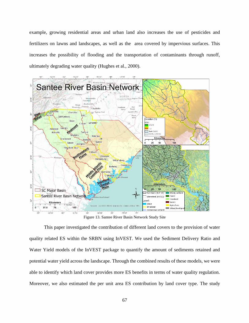
67
example, growing residential areas and urban land also increases the use of pesticides and
fertilizers on lawns and landscapes, as well as the area covered by impervious surfaces. This
increases the possibility of flooding and the transportation of contaminants through runoff,
ultimately degrading water quality (Hughes et al., 2000).
Figure 13. Santee River Basin Network Study Site
This paper investigated the contribution of different land covers to the provision of water
quality related ES within the SRBN using InVEST. We used the Sediment Delivery Ratio and
Water Yield models of the InVEST package to quantify the amount of sediments retained and
potential water yield across the landscape. Through the combined results of these models, we were
able to identify which land cover provides more ES benefits in terms of water quality regulation.
Moreover, we also estimated the per unit area ES contribution by land cover type. The study
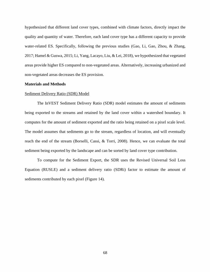
68
hypothesized that different land cover types, combined with climate factors, directly impact the
quality and quantity of water. Therefore, each land cover type has a different capacity to provide
water-related ES. Specifically, following the previous studies (Gao, Li, Gao, Zhou, & Zhang,
2017; Hamel & Guswa, 2015; Li, Yang, Lacayo, Liu, & Lei, 2018), we hypothesized that vegetated
areas provide higher ES compared to non-vegetated areas. Alternatively, increasing urbanized and
non-vegetated areas decreases the ES provision.
Materials and Methods
Sediment Delivery Ratio (SDR) Model
The InVEST Sediment Delivery Ratio (SDR) model estimates the amount of sediments
being exported to the streams and retained by the land cover within a watershed boundary. It
computes for the amount of sediment exported and the ratio being retained on a pixel scale level.
The model assumes that sediments go to the stream, regardless of location, and will eventually
reach the end of the stream (Borselli, Cassi, & Torri, 2008). Hence, we can evaluate the total
sediment being exported by the landscape and can be sorted by land cover type contribution.
To compute for the Sediment Export, the SDR uses the Revised Universal Soil Loss
Equation (RUSLE) and a sediment delivery ratio (SDRi) factor to estimate the amount of
sediments contributed by each pixel (Figure 14).
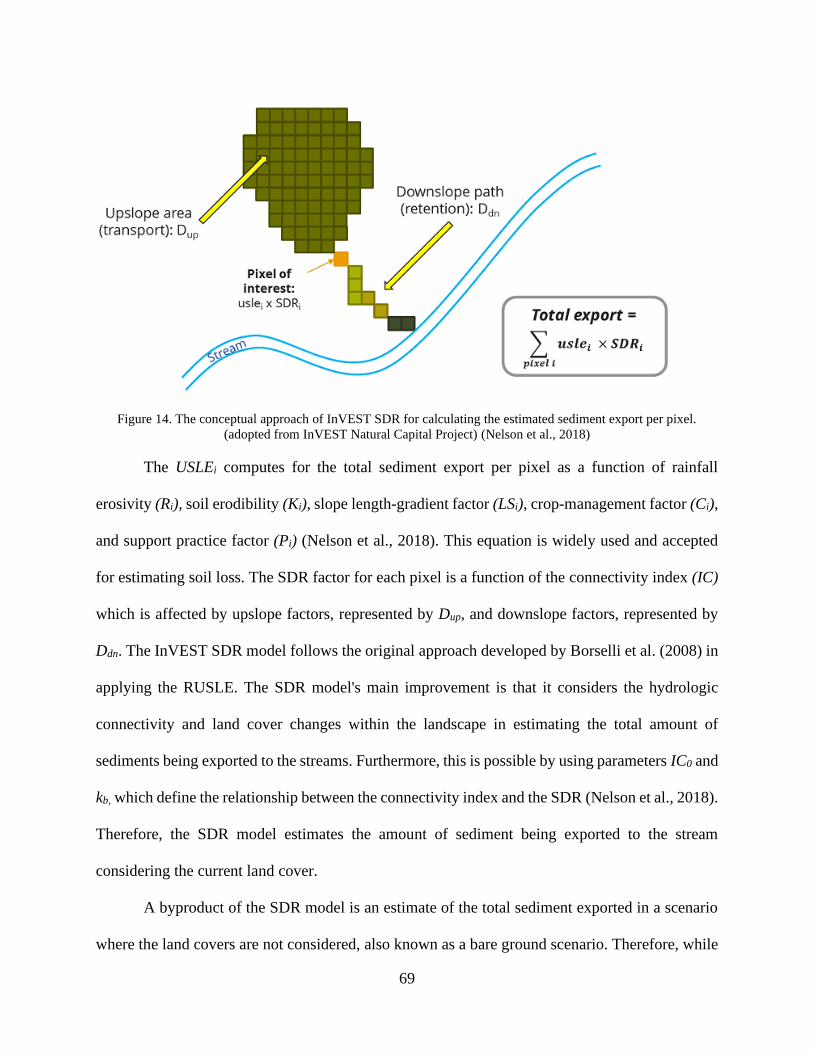
69
Figure 14. The conceptual approach of InVEST SDR for calculating the estimated sediment export per pixel.
(adopted from InVEST Natural Capital Project) (Nelson et al., 2018)
The USLEi computes for the total sediment export per pixel as a function of rainfall
erosivity (Ri), soil erodibility (Ki), slope length-gradient factor (LSi), crop-management factor (Ci),
and support practice factor (Pi) (Nelson et al., 2018). This equation is widely used and accepted
for estimating soil loss. The SDR factor for each pixel is a function of the connectivity index (IC)
which is affected by upslope factors, represented by Dup, and downslope factors, represented by
Ddn. The InVEST SDR model follows the original approach developed by Borselli et al. (2008) in
applying the RUSLE. The SDR model's main improvement is that it considers the hydrologic
connectivity and land cover changes within the landscape in estimating the total amount of
sediments being exported to the streams. Furthermore, this is possible by using parameters IC0 and
kb, which define the relationship between the connectivity index and the SDR (Nelson et al., 2018).
Therefore, the SDR model estimates the amount of sediment being exported to the stream
considering the current land cover.
A byproduct of the SDR model is an estimate of the total sediment exported in a scenario
where the land covers are not considered, also known as a bare ground scenario. Therefore, while

70
the SDR model focuses on estimating the sediments being exported to the stream, this can also be
used to compute the amount of sediment being retained by the land cover. The difference between
the sediment export with the land cover and the sediment export with the bare ground scenario,
results in the amount of sediments retained by the land cover. This contributes to the water quality
regulation which was the focus of this study.
Water Yield (WY) Model
The InVEST Water Yield (WY) model is the module for estimating the potential volume
of water that a land cover can capture from rain events. While the model is originally intended for
hydropower production, the information for quantifying the amount of water is still useful for
analyzing the land cover contribution to surface water (Nelson et al., 2018; Redhead et al., 2016).
Figure 15. Visualization of the InVEST WY framework for computing water yield potential per pixel
(adopted from InVEST Natural Capital Project) (Nelson et al., 2018)
The WY model framework (Figure 15) is based on the Budyko curve and average
precipitation to estimate the amount of potential water yield per pixel (Nelson et al., 2018). The
model estimates the actual evapotranspiration, AET(x), and subtracts it from the total amount of

71
water from precipitation, P(x), that a pixel receives. The AET is derived based on the Budyko
curve (Fu, 1981; Zhang et al., 2004) using the parameters potential evapotranspiration, PET(x),
and w(x), which is a non-physical parameter for climatic-soil properties (Nelson et al., 2018). The
w(x) is a function of the volumetric plant available water capacity of the soil, AWC(x); the average
precipitation, P(x), and an empirical constant Z which captures the local precipitation pattern and
hydrogeological characteristics (Nelson et al., 2018; Redhead et al., 2016; Yang et al., 2019).
The WY model estimates can provide different information about the landscape’s water
yield potential. Depending on the spatial scale of the analysis, the estimates can be interpreted
differently. For example, estimating the total water yield that can be gathered by the overall area
can be interpreted as the potential contribution of the landscape to the water supply. Therefore, a
higher overall water yield potential will result in a benefit and an improvement of the ES
(Canqiang, Wenhua, Biao, & Moucheng, 2012; Yang et al., 2019). However, if the WY potential
estimate is assessed per land cover or per unit area, the amount of water that each pixel retained
after a rain event is expected to be released to the streams through surface runoff (Gao et al., 2017;
Lang, Song, & Zhang, 2017; Li et al., 2018; Nelson et al., 2018). Hence, a higher WY potential
per unit area will indicate a higher likelihood of surface runoff. Consequently, in a per area and
per land cover analysis, a lower WY potential will indicate in a lower possibility of surface runoff,
thus implying an improvement of ES.
Data Requirements
The InVEST models’ data requirements are mainly spatially explicit files and a tabular
dataset that corresponds to the biophysical characteristics per land cover. Table 10 lists the details
of the data inputs for the SDR and WY models.
Table 10. List of required data inputs for the InVEST models
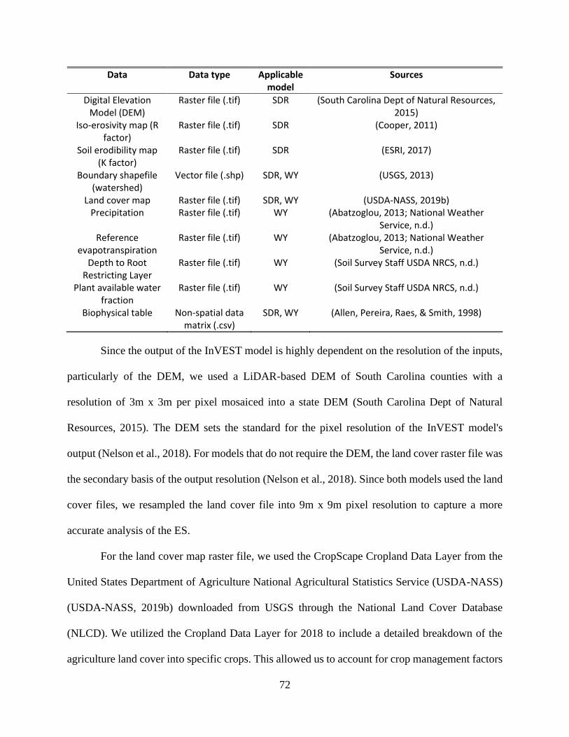
72
Data Data type Applicable model
Sources
Digital Elevation Model (DEM)
Raster file (.tif) SDR (South Carolina Dept of Natural Resources, 2015)
Iso-erosivity map (R factor)
Raster file (.tif) SDR (Cooper, 2011)
Soil erodibility map (K factor)
Raster file (.tif) SDR (ESRI, 2017)
Boundary shapefile (watershed)
Vector file (.shp) SDR, WY (USGS, 2013)
Land cover map Raster file (.tif) SDR, WY (USDA-NASS, 2019b) Precipitation Raster file (.tif) WY (Abatzoglou, 2013; National Weather
Service, n.d.) Reference
evapotranspiration Raster file (.tif) WY (Abatzoglou, 2013; National Weather
Service, n.d.) Depth to Root
Restricting Layer Raster file (.tif) WY (Soil Survey Staff USDA NRCS, n.d.)
Plant available water fraction
Raster file (.tif) WY (Soil Survey Staff USDA NRCS, n.d.)
Biophysical table Non-spatial data matrix (.csv)
SDR, WY (Allen, Pereira, Raes, & Smith, 1998)
Since the output of the InVEST model is highly dependent on the resolution of the inputs,
particularly of the DEM, we used a LiDAR-based DEM of South Carolina counties with a
resolution of 3m x 3m per pixel mosaiced into a state DEM (South Carolina Dept of Natural
Resources, 2015). The DEM sets the standard for the pixel resolution of the InVEST model's
output (Nelson et al., 2018). For models that do not require the DEM, the land cover raster file was
the secondary basis of the output resolution (Nelson et al., 2018). Since both models used the land
cover files, we resampled the land cover file into 9m x 9m pixel resolution to capture a more
accurate analysis of the ES.
For the land cover map raster file, we used the CropScape Cropland Data Layer from the
United States Department of Agriculture National Agricultural Statistics Service (USDA-NASS)
(USDA-NASS, 2019b) downloaded from USGS through the National Land Cover Database
(NLCD). We utilized the Cropland Data Layer for 2018 to include a detailed breakdown of the
agriculture land cover into specific crops. This allowed us to account for crop management factors
73
and support practice factor for the SDR model. For the WY model, we also included a crop
coefficient for predicting evapotranspiration (Allen et al., 1998; Nelson et al., 2018).
Specifically for the SDR model data requirements, the Iso-erosivity map was derived using
Renard and Fremund (1994) equation for Coterminous US (Cooper, 2011) which was converted
from US customary units into metric units (MJ/ha) to adhere to the model specifications (Nelson
et al., 2018). Furthermore, the soil erodibility map, downloaded through ArcGIS Online (ESRI,
2017), was also converted into metric units ((tons * ha * hr) / (ha * MJ* mm)) as per model
specification (Nelson et al., 2018). Finally, a comma-separated value (.csv) file containing the crop
management factor and support practice factor per land cover was used for the RUSLE
computation obtained from the Food and Agriculture Organization (FAO) (Allen et al., 1998).
For the WY model, the precipitation and reference evapotranspiration raster files were
obtained from Climatology Lab (Abatzoglou, 2013) and the National Oceanic and Atmospheric
Administration (NOAA) (National Weather Service, n.d.). The depth to root restricting layer and
plant available water fraction raster files were obtained through the Soil Survey Geographic
Database (SSURGO) (Soil Survey Staff USDA NRCS, n.d.). Lastly, a comma-separated value
(.csv) file containing the crop coefficient (Kc) by land cover was used as a constant multiplier for
computing w in the WY model.
All spatial data inputs were delineated using the Hydrologic Unit Classification 12 (HUC
12) obtained from the watershed boundary dataset (WBD) (USGS, 2013) and aggregated as Santee
River Basin Network.
Modifying for crop seasonality
One of the limitations of the InVEST model is that it is a single-time analysis. Therefore,
it quantifies the ES on an annualized temporal scale using mean values of data inputs. This could
74
be a challenge, particularly for analyzing monthly and seasonal changes to ES. To address this, we
ran the InVEST models using parameters that simulated monthly events in the landscape, focusing
on the changes in the agriculture land cover.
Using a cropping calendar, we identified which crops are offseason per month. We
assumed that the offseason crops will have similar values to idle cropland; hence changing its crop
management factor, support practice factor, crop coefficient, and its interacting effects with the
monthly climate variables. This allowed for quantifying the monthly ES within the SRBN.
Furthermore, to account for the effect of the sustainable farming intervention, we ran the models
for each month while modifying the crop management factor, support practice factor, and crop
coefficient factor of the offseason crops into values based on cover crops.
Model limitation and calibration
The InVEST models are widely applied in the quantification of ES, particularly on a
landscape scale (Vigerstol & Aukema, 2011). One of its main assets is the model's spatial
characteristics and versatility using GIS as a platform. However, the models are not without their
limitation. It can only quantify for a single time period; hence, losing the effect of the temporal
changes (Bagstad, Cohen, Ancona, McNulty, & Sun, 2018; Redhead et al., 2016; Sharps et al.,
2017). Furthermore, the results of the InVEST model are heavily dependent on the quality of inputs
that are used. Inputs with refined spatial resolution yield more accurate and precise results, while
coarse spatial resolution datasets are more prone to overestimation and focused more on regional
landscape analyses (Bagstad, Semmens, & Winthrop, 2013; Dennedy-Frank, Muenich, Chaubey,
& Ziv, 2016; Redhead et al., 2016; Sharps et al., 2017; J. C. Ureta, Zurqani, Post, Ureta, &
Motallebi, 2020).
75
Moreover, there is limited literature that compared the InVEST model results with
observed data, making it difficult to validate (Yang et al., 2019). The InVEST models simplify the
application of hydrology and geomorphology equations on a landscape scale. Depending on the
amount of details present in the spatial dataset, the models are prone to standardizing and averaging
of parameters across the landscape. This means that the parameters used in one region will be the
same across all the regions as long as they are of similar land cover type, which in reality is not
true. For example, the crop coefficients of a specific crop can differ between an upland and lowland
area. However, due to the standardization of parameters, the model uses the same multiplier on
that particular crop regardless of geographic location. Therefore, to address this, the model must
be calibrated against actual observed flow and sediment values from monitoring stations (Bagstad
et al., 2018; Redhead et al., 2016; Vigerstol & Aukema, 2011).
Finally, for the water yield model, the estimated water yield potential accounts for the total
volume of water that can be captured by the land cover (Canqiang et al., 2012; Li et al., 2018;
Nelson et al., 2018). Part of this volume will infiltrate and contribute to the water supply, but a
substantial amount will become a runoff (Nelson et al., 2018). The current WY model does not
have the capacity to separate between the volume that infiltrates and becomes a surface runoff.
While the aggregated water yield potential across the watershed can be interpreted as a total
contribution to water supply, the per unit area estimation can be construed more likely as a surface
runoff.
Calibrating the model
For calibration purposes, we ran the InVEST models with the same catchment size as the
benchmark stations. We adjusted the model parameters until they produced similar quantities as
with the benchmark. The actual flow rate readings were used for the WY calibration benchmark,

76
while a sediment deposition estimate (McCarney-Castle, Childress, & Heaton, 2017) was used for
the SDR calibration. We based the calibration of the SDR model from the measurement of
McCarney-Castle et al. (2017), while the WY model was based on the National Water Information
System (NWIS). Both were conducted in the Lawsons Fork Creek, Spartanburg, South Carolina.
The observed annual average sediment yield in Lawsons Fork Creek amounted to 168 tons/km2
(McCarney-Castle et al., 2017). This served as a benchmark to calibrate the InVEST SDR model
while adjusting the parameters IC0 and kb. Following the SDR model documentation, we set the
IC0 to its default value (0.5) and adjusted the kb parameter (Nelson et al., 2018). We ran different
model iterations using different kb parameter values to produce a closely similar estimate to
McCarney-Castle et al. (2017). We determined that a kb value of 0.95 – 0.96 produced an estimate
that was not statistically different from the observed value of McCarney-Castle et al. (2017).
In the same way for the WY model, we used the observed value of 22.53 m/m2/year or a
total of 4.3 billion cubic meters per year (USGS, n.d.-b) as a benchmark for calibration. The WY
model uses an empirical constant Z, which represents the seasonal distribution of precipitation. We
calibrated the Z value by comparing the modeled and observed data to show the sensitivity of the
model to the empirical constant (Nelson et al., 2018). A higher Z value suggests that the sensitivity
of the model to the constant is lower (Zhang et al., 2004). One way to estimate the Z parameter is
by multiplying the number of rain events per year to 0.2 constant (Donohue, Roderick, & McVicar,
2012; Hamel & Guswa, 2015). Therefore, we determined an appropriate Z value of 22 for the
Lawsons Fork Creek. In addition, since the WY model is also highly sensitive to variability in
precipitation, it is expected that there will be a difference between the observed water yield and
the model result (Hamel & Guswa, 2015). Following the results of the sensitivity analysis, we

77
increased the value of the precipitation data inputs by 9%. Using these calibrated parameters, the
model estimated a water yield that was not statistically different from the observed value.
Results
Land cover change in SRBN
A land cover change analysis between 2016 and 2001 land cover maps (Figure 16) showed
that around 200,000 acres (2.5%) of the vegetated land covers in SRBN – including forest land,
agriculture, grassland, and wetlands – was converted to developed or urban land cover
classification (USGS, n.d.-a). While the percent change of the vegetated land cover seems to be
relatively small, the effect on the ecosystems can still be significant.
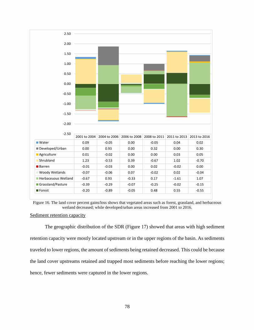
78
Figure 16. The land cover percent gains/loss shows that vegetated areas such as forest, grassland, and herbaceous
wetland decreased; while developed/urban areas increased from 2001 to 2016.
Sediment retention capacity
The geographic distribution of the SDR (Figure 17) showed that areas with high sediment
retention capacity were mostly located upstream or in the upper regions of the basin. As sediments
traveled to lower regions, the amount of sediments being retained decreased. This could be because
the land cover upstreams retained and trapped most sediments before reaching the lower regions;
hence, fewer sediments were captured in the lower regions.
2001 to 2004 2004 to 2006 2006 to 2008 2008 to 2011 2011 to 2013 2013 to 2016
Water 0.09 -0.05 0.00 -0.05 0.04 0.02
Developed/Urban 0.00 0.93 0.00 0.32 0.00 0.30
Agriculture 0.01 -0.02 0.00 0.00 0.03 0.05
Shrubland 1.23 -0.53 0.39 -0.67 1.02 -0.70
Barren -0.01 -0.03 0.00 0.02 -0.02 0.00
Woody Wetlands -0.07 -0.06 0.07 -0.02 0.02 -0.04
Herbaceuous Wetland -0.67 0.93 -0.33 0.17 -1.61 1.07
Grassland/Pasture -0.39 -0.29 -0.07 -0.25 -0.02 -0.15
Forest -0.20 -0.89 -0.05 0.48 0.55 -0.55
-2.50
-2.00
-1.50
-1.00
-0.50
0.00
0.50
1.00
1.50
2.00
2.50
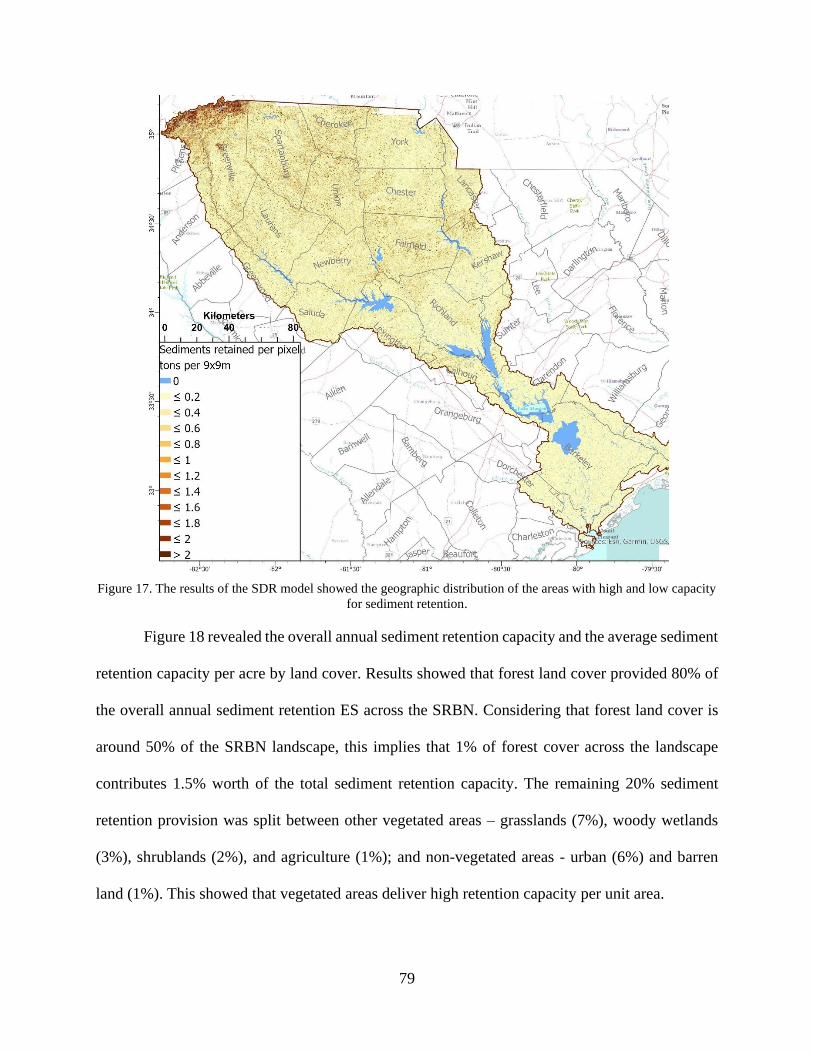
79
Figure 17. The results of the SDR model showed the geographic distribution of the areas with high and low capacity
for sediment retention.
Figure 18 revealed the overall annual sediment retention capacity and the average sediment
retention capacity per acre by land cover. Results showed that forest land cover provided 80% of
the overall annual sediment retention ES across the SRBN. Considering that forest land cover is
around 50% of the SRBN landscape, this implies that 1% of forest cover across the landscape
contributes 1.5% worth of the total sediment retention capacity. The remaining 20% sediment
retention provision was split between other vegetated areas – grasslands (7%), woody wetlands
(3%), shrublands (2%), and agriculture (1%); and non-vegetated areas - urban (6%) and barren
land (1%). This showed that vegetated areas deliver high retention capacity per unit area.

80
Figure 18. The annual total sediments retained per land cover in SRBN showed that the forest land provide the most
sediment retention capacity, while the mean sediments retained showed that vegetated areas including the forest,
grassland, shrubland, wetland, and agriculture provide a high sediment retention capacity for water quality
regulation.
An analysis of the per acre contribution by land cover showed the efficiency of each land
cover in retaining the sediments (Figure 18). Results indicated that forest land cover has the highest
retention capacity with a mean of 3,400 tons of sediments per acre annually. Furthermore, the
overall mean sediments retained per acre of other vegetated areas amounted to 3,980 tons per acre,
while the non-vegetated areas amounted to 3,480 tons per acre.
Area in (acres)Total annual sediments
retained ('000 tons)
Mean sediment retainedper area
(tons / acre)
Water 19,992 5,853 293
Shrubland 20,668 23,424 1,133
Herbaceous Wetland 5,875 794 135
Woody Wetland 53,037 30,712 579
Forest 245,088 843,236 3,441
Grassland/Pasture 51,231 80,952 1,580
Offseason cropland 0 - -
Idle Cropland 924 554 599
Barren 2,164 3,652 1,687
Agriculture 18,017 9,954 553
Developed/Urban 62,341 74,522 1,195
0%
10%
20%
30%
40%
50%
60%
70%
80%
90%
100%
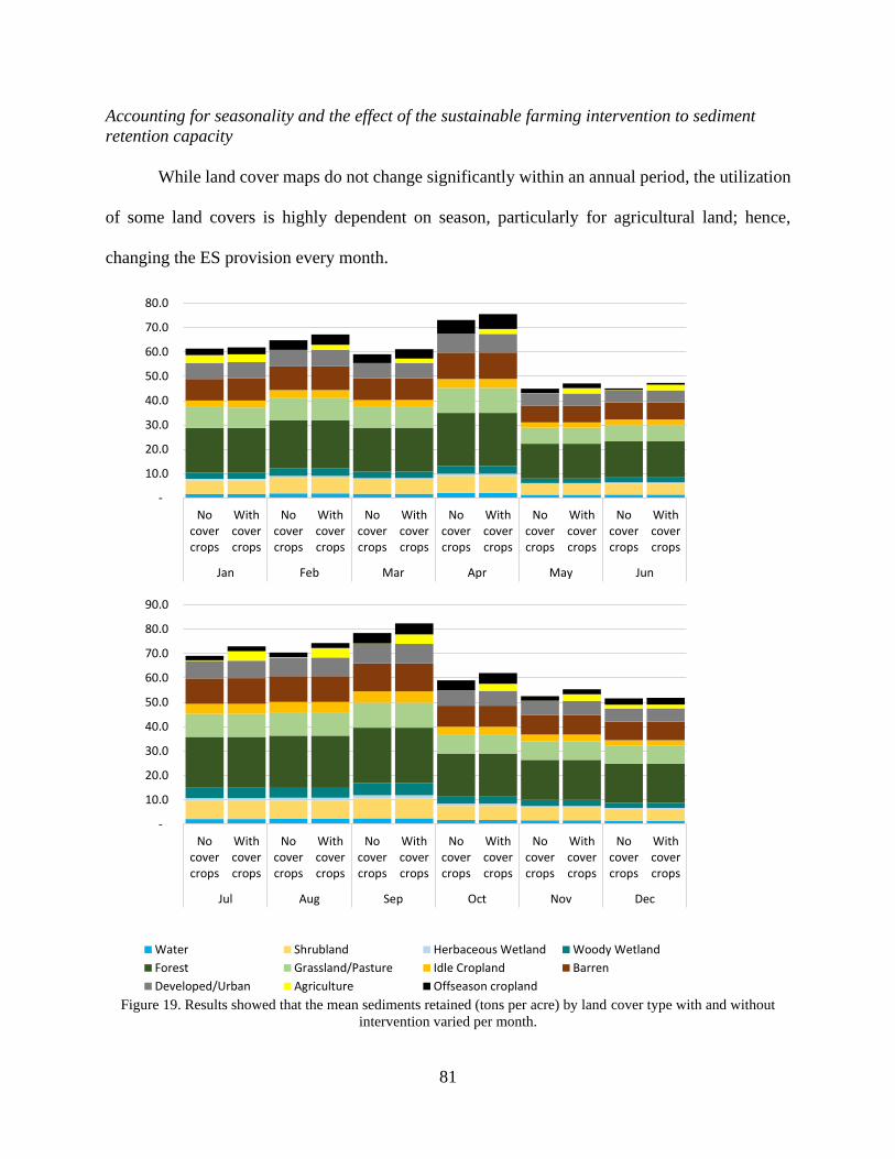
81
Accounting for seasonality and the effect of the sustainable farming intervention to sediment
retention capacity
While land cover maps do not change significantly within an annual period, the utilization
of some land covers is highly dependent on season, particularly for agricultural land; hence,
changing the ES provision every month.
Figure 19. Results showed that the mean sediments retained (tons per acre) by land cover type with and without
intervention varied per month.
-
10.0
20.0
30.0
40.0
50.0
60.0
70.0
80.0
Nocovercrops
Withcovercrops
Nocovercrops
Withcovercrops
Nocovercrops
Withcovercrops
Nocovercrops
Withcovercrops
Nocovercrops
Withcovercrops
Nocovercrops
Withcovercrops
Jan Feb Mar Apr May Jun
-
10.0
20.0
30.0
40.0
50.0
60.0
70.0
80.0
90.0
Nocovercrops
Withcovercrops
Nocovercrops
Withcovercrops
Nocovercrops
Withcovercrops
Nocovercrops
Withcovercrops
Nocovercrops
Withcovercrops
Nocovercrops
Withcovercrops
Jul Aug Sep Oct Nov Dec
Water Shrubland Herbaceous Wetland Woody Wetland
Forest Grassland/Pasture Idle Cropland Barren
Developed/Urban Agriculture Offseason cropland
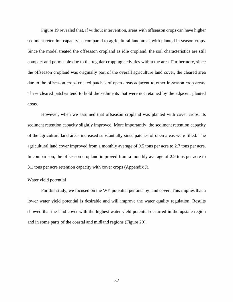
82
Figure 19 revealed that, if without intervention, areas with offseason crops can have higher
sediment retention capacity as compared to agricultural land areas with planted in-season crops.
Since the model treated the offseason cropland as idle cropland, the soil characteristics are still
compact and permeable due to the regular cropping activities within the area. Furthermore, since
the offseason cropland was originally part of the overall agriculture land cover, the cleared area
due to the offseason crops created patches of open areas adjacent to other in-season crop areas.
These cleared patches tend to hold the sediments that were not retained by the adjacent planted
areas.
However, when we assumed that offseason cropland was planted with cover crops, its
sediment retention capacity slightly improved. More importantly, the sediment retention capacity
of the agriculture land areas increased substantially since patches of open areas were filled. The
agricultural land cover improved from a monthly average of 0.5 tons per acre to 2.7 tons per acre.
In comparison, the offseason cropland improved from a monthly average of 2.9 tons per acre to
3.1 tons per acre retention capacity with cover crops (Appendix J).
Water yield potential
For this study, we focused on the WY potential per area by land cover. This implies that a
lower water yield potential is desirable and will improve the water quality regulation. Results
showed that the land cover with the highest water yield potential occurred in the upstate region
and in some parts of the coastal and midland regions (Figure 20).

83
Figure 20. The results of the InVEST WY model showed that the highlighted blue areas have the highest water yield
potential per pixel, while the green areas have the lowest.
The blue areas coincide with the urban/developed areas of the land cover map. This is
supported by the results in Figure 21 showing that urban/developed land cover accounted for most
(46%) of the estimated total annual water yield potential. However, considering that
urban/developed land cover accounted for only 13% of the overall land cover, the ratio of the
amount of water yield potential per area was around three times more than a forested land cover
area.
Similarly, urban/developed land cover areas had the highest mean water yield potential
among the different land cover types. Likewise, other non-vegetated areas such as barren land and
idle cropland recorded a high mean water yield potential per area. While these land cover types
are not impervious, there is little vegetation that can consume and hold the water.
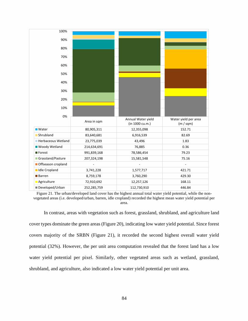
84
Figure 21. The urban/developed land cover has the highest annual total water yield potential, while the non-
vegetated areas (i.e. developed/urban, barren, idle cropland) recorded the highest mean water yield potential per
area.
In contrast, areas with vegetation such as forest, grassland, shrubland, and agriculture land
cover types dominate the green areas (Figure 20), indicating low water yield potential. Since forest
covers majority of the SRBN (Figure 21), it recorded the second highest overall water yield
potential (32%). However, the per unit area computation revealed that the forest land has a low
water yield potential per pixel. Similarly, other vegetated areas such as wetland, grassland,
shrubland, and agriculture, also indicated a low water yield potential per unit area.
Area in sqmAnnual Water yield
(in 1000 cu.m.)Water yield per area
(m / sqm)
Water 80,905,311 12,355,098 152.71
Shrubland 83,640,681 6,916,539 82.69
Herbaceous Wetland 23,775,039 43,496 1.83
Woody Wetland 214,634,691 76,885 0.36
Forest 991,839,168 78,586,454 79.23
Grassland/Pasture 207,324,198 15,581,548 75.16
Offseason cropland - - -
Idle Cropland 3,741,228 1,577,717 421.71
Barren 8,759,178 3,760,290 429.30
Agriculture 72,910,692 12,257,126 168.11
Developed/Urban 252,285,759 112,730,910 446.84
0%
10%
20%
30%
40%
50%
60%
70%
80%
90%
100%
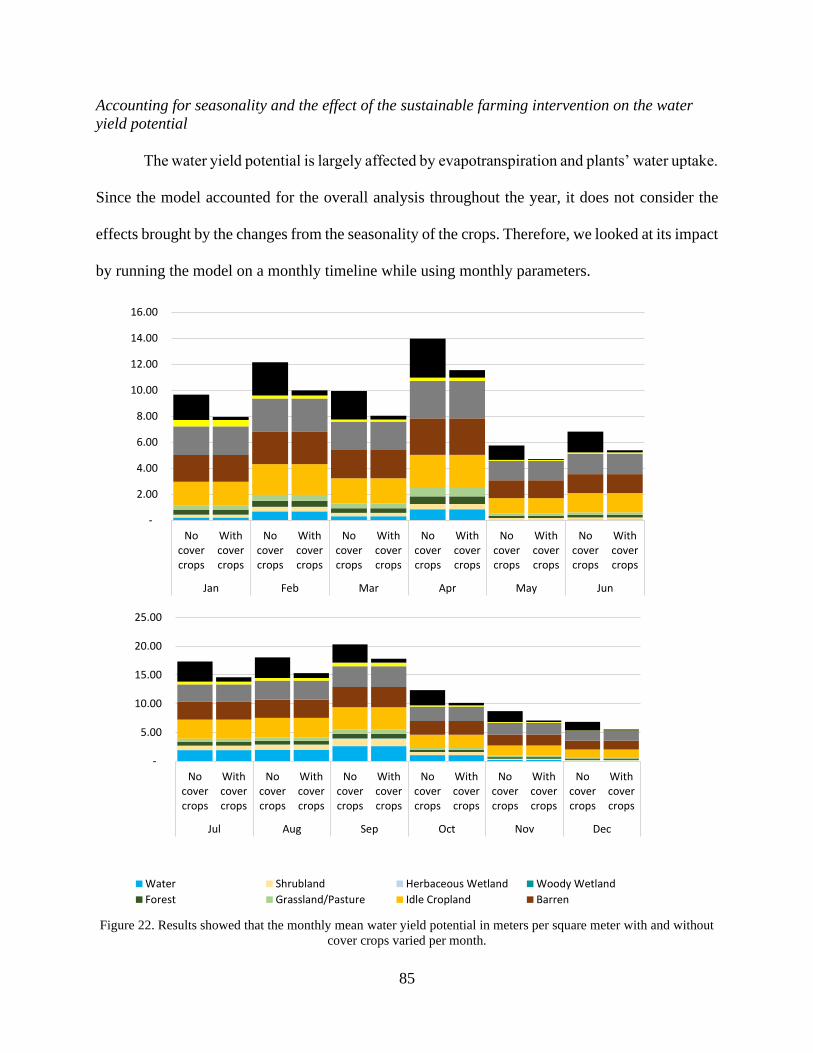
85
Accounting for seasonality and the effect of the sustainable farming intervention on the water
yield potential
The water yield potential is largely affected by evapotranspiration and plants’ water uptake.
Since the model accounted for the overall analysis throughout the year, it does not consider the
effects brought by the changes from the seasonality of the crops. Therefore, we looked at its impact
by running the model on a monthly timeline while using monthly parameters.
Figure 22. Results showed that the monthly mean water yield potential in meters per square meter with and without
cover crops varied per month.
-
2.00
4.00
6.00
8.00
10.00
12.00
14.00
16.00
Nocovercrops
Withcovercrops
Nocovercrops
Withcovercrops
Nocovercrops
Withcovercrops
Nocovercrops
Withcovercrops
Nocovercrops
Withcovercrops
Nocovercrops
Withcovercrops
Jan Feb Mar Apr May Jun
-
5.00
10.00
15.00
20.00
25.00
Nocovercrops
Withcovercrops
Nocovercrops
Withcovercrops
Nocovercrops
Withcovercrops
Nocovercrops
Withcovercrops
Nocovercrops
Withcovercrops
Nocovercrops
Withcovercrops
Jul Aug Sep Oct Nov Dec
Water Shrubland Herbaceous Wetland Woody Wetland
Forest Grassland/Pasture Idle Cropland Barren

86
Figure 22 showed that without intervention, the offseason cropland has a high amount of
mean water yield potential that was almost similar to non-vegetated areas such as barren and idle
cropland. With intervention, the monthly water yield potential per unit area of offseason cropland
significantly decreased by 83% on the average (Appendix K).
Furthermore, the non-vegetated areas (i.e. urban/developed, barren, and idle cropland) has
the highest water yield potential per unit area, particularly in the upper region, followed by the
coastal or Lowcountry region, and lastly by the midland region. On the other hand, vegetated areas
(i.e. forest, grassland, shrubland, and agriculture) have low water yield potential per unit area due
to the uptake of water by the vegetation.
Discussion
The land cover change analysis showed that the land conversion of vegetated areas to non-
vegetated areas is continuing. Notably, a substantial amount of forest, wetland, and shrubland are
being converted into urban/developed areas. A similar pattern was also observed in a land cover
analysis of contiguous US from 2001- 2011 (J. Chen, Theller, Gitau, Engel, & Harbor, 2017).
These land conversions affect the ecosystems, and ES produced within the landscape. Therefore,
if the trend of urban areas continuously expands while vegetated areas continue to decline, this can
lead to irreversible damage to the ecosystems and their services.
The forest land cover has the highest sediment retention capacity across the landscape.
Since forested areas host a diverse composition of plants and trees, this holds together soil organic
matter and contributes to the retention of sediments and prevention of soil erosion. Therefore,
keeping the forest land intact ensures the continuous provision of ES. A similar observation was
also found in a previous study about the sediment retention by natural landscapes in the US
(Woznicki et al., 2020). This reinforces the need for more forest conservation and management
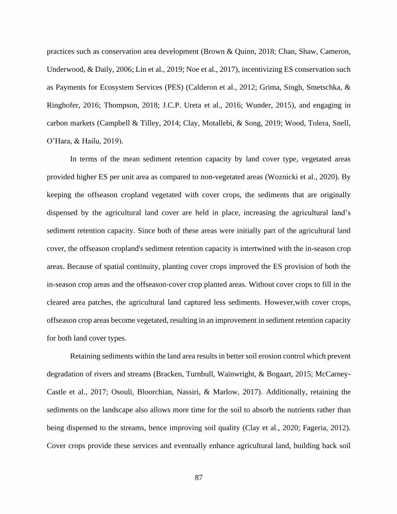
87
practices such as conservation area development (Brown & Quinn, 2018; Chan, Shaw, Cameron,
Underwood, & Daily, 2006; Lin et al., 2019; Noe et al., 2017), incentivizing ES conservation such
as Payments for Ecosystem Services (PES) (Calderon et al., 2012; Grima, Singh, Smetschka, &
Ringhofer, 2016; Thompson, 2018; J.C.P. Ureta et al., 2016; Wunder, 2015), and engaging in
carbon markets (Campbell & Tilley, 2014; Clay, Motallebi, & Song, 2019; Wood, Tolera, Snell,
O’Hara, & Hailu, 2019).
In terms of the mean sediment retention capacity by land cover type, vegetated areas
provided higher ES per unit area as compared to non-vegetated areas (Woznicki et al., 2020). By
keeping the offseason cropland vegetated with cover crops, the sediments that are originally
dispensed by the agricultural land cover are held in place, increasing the agricultural land’s
sediment retention capacity. Since both of these areas were initially part of the agricultural land
cover, the offseason cropland's sediment retention capacity is intertwined with the in-season crop
areas. Because of spatial continuity, planting cover crops improved the ES provision of both the
in-season crop areas and the offseason-cover crop planted areas. Without cover crops to fill in the
cleared area patches, the agricultural land captured less sediments. However,with cover crops,
offseason crop areas become vegetated, resulting in an improvement in sediment retention capacity
for both land cover types.
Retaining sediments within the land area results in better soil erosion control which prevent
degradation of rivers and streams (Bracken, Turnbull, Wainwright, & Bogaart, 2015; McCarney-
Castle et al., 2017; Osouli, Bloorchian, Nassiri, & Marlow, 2017). Additionally, retaining the
sediments on the landscape also allows more time for the soil to absorb the nutrients rather than
being dispensed to the streams, hence improving soil quality (Clay et al., 2020; Fageria, 2012).
Cover crops provide these services and eventually enhance agricultural land, building back soil

88
organic matter and increasing the viability of agricultural land for both ES and cash crop yields.
This suggests that using cover crops as sustainable farming practice improves water quality
regulation across the landscape.
In terms of the geographic location, results of the InVEST SDR model showed that the
upstate region of SRBN has a high sediment retention capacity. The upstate region has
mountainous and densely vegetated areas; therefore, sediments are retained primarily in those
areas. Since sediments are captured and trapped in the upstate region, fewer sediment travels
downstream, hence expecting lower sediment retention capacity from the lower regions.
When it comes to water yield potential, urban/developed areas recorded the highest estimates
among different land cover types. This high potential water yield can be due to the characteristics
of the urban land since it has many impervious areas. These areas have low to no
evapotranspiration and infiltration capacity; hence, the water yield from these areas will move
across the landscape as surface runoff. This result is consistent with the previous studies on the
impact of urbanization on surface runoff (J. Chen et al., 2017; Hung, James, & Carbone, 2018).
Similar to non-vegetated areas like idle cropland and barren land cover, urban/developed areas
have little or no plant water uptake. Hence, when an agricultural land is not in use such as the case
of offseason cropland, its potential water yield per unit area also increases, as well as the possibility
of runoff, erosion, and sediment export. This will eventually affect the water quality of nearby
streams, rivers, and other water bodies.
In contrast, vegetated land cover types such as forest, grassland, shrubland, and in-season
agriculture land recorded low water yield potential per unit area because of the plants’ water
uptake. The decrease in the water yield potential per unit area implies a reduction in surface runoff.
Since vegetative root systems hold soil in place, the vegetation's presence also improves soil
89
organic matter within the area. In addition, low runoff implied from a low water yield potential
can mean a reduced possibility of flooding. Overall, this improves the water quality of nearby
water bodies and enhances soil quality, which ultimately can reduce the farm input costs and
improve contribution to flood control (J. C. Ureta, Zurqani, et al., 2020; Ward, Tockner, &
Schiemer, 1999; Zurqani et al., 2020). Therefore, the implementation of cover crops as a
sustainable farming practice can improve the ES across the landscape. In contrast, the decline of
vegetated land cover can result in decreased ES.
Finally, the upstate region of SRBN recorded the highest water yield potential across the
landscape. Since most of the headwaters are typically found in this region, it serves as a
precipitation catch basin. On the other hand, most streams and rivers eventually converge in coastal
areas, thus accumulating a substantial amount of water yield potential for this region. Although
the midland region has the lowest potential water yield, the InVEST WY model showed high water
yield potential in some areas, particularly in highly urbanized locations.
Conclusion
This study quantified the ES, particularly the sediment retention capacity and water yield
potential of the different land cover types of the Santee River Basin Network (SRBN). The InVEST
Sediment Delivery Ratio (SDR) model was used to estimate the amount of sediments being
retained per unit area by each land cover type. Additionally, the InVEST Water Yield (WY) model
quantified the potential volume of water yield per unit area. Since the per unit area analysis
represents the volume that can be a potential surface runoff, this implies that areas with low water
yield generate higher ES.
In both models, results showed that vegetated areas provide more ES, particularly the forest
land cover type. This means that keeping the forest intact and conserved is critical in continuous
90
ES provision. Also, since areas with offseason cropland perform as idle cropland, monthly changes
in agricultural systems that create cleared area patches adversely affect the delivery of ES. This
increases landscape susceptibility to erosion and decline in water quality. In contrast, application
of sustainable practices such as planting of cover crops in offseason cropland ensures the
continuous provision of the ES. This can eventually translate into cost savings for farmers as it
will retain the nutrients needed for planting the next season crops, avoiding unnecessary costs of
additional fertilizers.
The study also showed that conservation programs and sustainable farming practices, such
as cover crop implementation, provides benefits such as soil health improvement, water quality
regulation, and continuous provision of water-related ES by keeping the land vegetated. This
reinforces the need for more conservation programs and sustainable financing mechanisms to
enhance soil conservation in agriculture systems and forest protection, such as the Payments for
Ecosystem Services (PES).
The methods applied in this study could potentially be used to design a PES framework
within the basin. Since the willingness-to-pay (WTP) or financing support of ES buyers is tied up
to the product that they expect to receive (Fauzi & Anna, 2013; Mercer et al., 2011; Thompson,
2018; J.C.P. Ureta et al., 2016), quantifying the ES provided by the land cover gives clear
information on what ES sellers should deliver. On the other hand, knowing the ES benefits helps
the ES sellers choose the appropriate intervention that would maximize the ES. Therefore,
quantifying the amount of ES improvement provided by sustainable agricultural practices and
conservation programs also estimates the potential value of the benefits of these practices.
Finally, the map of ES generated from this study can provide spatial information about the
hotspots of prime areas for ES conservation. For example, integrating the geographic location and
91
the effect of land cover types on ES quantification showed that urban/developed areas in the upper
region provided low sediment retention capacity and high water yield potential. This could pose a
threat to ecosystem conservation and landscape sustainability planning. However, threats could be
mitigated with proper management and conservation of forest land, especially those surrounding
the urban/developed land. Furthermore, the quantification of ES can also be used to analyze the
effect of sustainable practices on ES delivery. The continuous provision of ES is critical to
society’s well-being. Therefore, the results of this study can provide inputs and information
towards landscape sustainability planning and conservation management practices.
92
CHAPTER FOUR
VALUATION OF ECOSYSTEM SERVICE IMPROVEMENTS IN SANTEE RIVER BASIN
NETWORK
Introduction
Watershed management is a critical aspect of sustainable development. Watersheds hold
multiple ecosystems that benefit human well-being and produce many ecosystem services (ES)
(Millenium Ecosystem Assessment, 2005). Ecosystem services affect human well-being by
providing basic materials for health, security, and good social relations, ultimately allowing
individuals to choose to do what they value (Millenium Ecosystem Assessment, 2005). However,
over the last decades, urban and industrial expansion have been prioritized. Concurrently, as the
market pressure increases, the rate of natural resource extraction and industrialized agricultural
practices further exacerbate the decline of ecosystems and ES quality. Although economic
development benefits society, if not properly managed often results in harmful tradeoffs to the
environment and decreased ES. Therefore, conservation programs and sustainable practices were
developed to protect specific ecosystems and ES to attain sustainable development.
The continuous provision of ES is generated by the ecosystem functions supported by the
biophysical processes (de Groot, Alkemade, Braat, Hein, & Willemen, 2010). Moreover, the
aggregation of these ecosystem functions makes up the landscape functions. Therefore, since the
land use-land cover (LULC) changes across the landscape impact the ecosystems, this affects the
provision of ES and alters the landscape functions.
A wide range of programs and farming practices are recognized for conservation and
sustainable development, such as agroforestry, cover crop planting, silviculture, contour farming,
permaculture designs, and conservation easements (Edwards, 1990). While many landowners and
farmers can implement these practices, the cost of implementation and the foregone immediate
93
economic benefits associated with these practices hinders widespread application (Hanson,
Hendrickson, & Archer, 2008). One approach to address this challenge is through sustainable
financing mechanisms such as the Payments for Ecosystem Services. These mechanisms provide
incentives to landowners and farmers to implement conservation programs and sustainable
practices.
Specifically, a Payments for Ecosystem Services (PES) program aims to support
conservation programs and sustainable practices to ensure a continuous flow of good quality
ecosystem services by providing a steady stream of financial resources. The fundamental principle
of a PES is that it is a voluntary transaction of a well-defined ES (or land-use likely to secure that
service) being ‘bought’ by a (minimum one) ES buyer from a (minimum one) ES provider and that
the ES provider guarantees the ES provision (Wunder, 2005). The program’s operational
foundation is that ES Providers, stakeholders that can manage the land which provides the
ecosystem services – also known as ES sellers, ensure the continuous provision of the ecosystem
services by maintaining healthy ecosystems within their land through conservation programs and
sustainable farming practices. On the other hand, ES Beneficiaries, stakeholders that directly
benefit or consume the ecosystem services – also known as ES buyers, support the ES sellers by
compensating their efforts in exchange for the continuous provision of ecosystem services.
A critical aspect for the success of a PES is that both ES sellers and ES buyers formalize
an agreement in which they will continue to support each other as long as the conditions are met
(Engel, Pagiola, & Wunder, 2008; Forest Trends et al., 2008; Wunder, 2005). This could either be
legally or non-legally binding as long as both parties are committed (Greiber, 2009). With this
conditionality, it is crucial to assess the willingness of all parties to participate by estimating the

94
willingness to pay of ES buyers that will support the providers and the willingness to accept of ES
sellers for implementing the conservation programs and sustainable practices in their land.
While the assessment of both ES Buyers and Sellers are equally important for designing a
PES, many studies are focused primarily on the sellers’ likelihood to participate in the scheme
(Cranford & Mourato, 2014; Ecoagriculture Partners, 2011; Jack, Kousky, & Sims, 2008; Vedel
et al., 2015; Zanella et al., 2014) and their adoption to conservation programs such as the USDA’s
Environmental Quality Incentives Program (EQIP), Wetlands Reserve Program (WRP), and
Conservation Stewardship Program (CSP) (USDA-NRCS, n.d.). On the other hand, although
works of literature about buyers’ participation in PES are available, since PES schemes are
location-specific and buyers’ support fuels the scheme, estimating the buyers’ willingness to pay
within the target PES site is critical in designing the program.
The present study is an effort to extend the related literature by assessing the residents’
value towards the improvement of ES within the Santee River Basin Network in South Carolina
(SRBN) and to provide comprehensive information on the feasibility of developing a PES in the
area. Estimating the residents’ value and determining the overall potential revenue across the
landscape could provide information if the PES scheme will be feasible to support the conservation
programs in the river basin.
The state of South Carolina (SC) is selected because urban areas have grown continuously
since 1970 (US Census, 2012; US Geological Survey (USGS) Gap Analysis Project (GAP), 2012).
Specifically within Santee River Basin Network (SRBN), the urban/developed land cover type
increased by 2.5% or approximately around 200,000 acres from 2001 to 2016 (Slade, 2018; J. C.
Ureta, Clay, Motallebi, & Ureta, 2020; US Census, 2012). With a population growth rate of 1.06%
estimated from 2010 to 2019 (“South Carolina Population 2019 (Demographics, Maps, Graphs),”
95
2019; United States Census Bureau, 2018), the expansion of urban/developed areas are expected
to continue. Since land use and land cover changes are highly affected by economic factors while
also affecting ecosystems, the continuous expansion of urban land cover is becoming detrimental
to ecosystem services. Therefore, it is imperative that land use management adheres to
sustainability standards to ensure the continuous provision of ES. This study aims to assess
residents' value towards the improvement of ES within the Santee River Basin Network (SRBN)
to provide comprehensive information on the feasibility of developing a PES in the area.
This study's primary objective is to estimate the residents’ willingness to pay for improving
the ecosystem services produced within the Santee River Basin Network (SRBN) and thereby
assess the viability of the PES for supporting conservation programs and sustainable practices.
Following the literature on ecosystem services preferences in South Carolina (J. C. Ureta,
Vassalos, Motallebi, Baldwin, & Ureta, 2020), we estimated the residents’ willingness-to-pay
(WTP) to improve water quality regulation, water supply provision, and wildlife habitat.
Furthermore, we determined the difference of WTP among residents from different regions of
SRBN using two sustainable practice interventions – cover crop and agroforestry.
Following the study of Ureta et al. (2020), since residents showed to have an understanding
of the importance of the ecosystem services to their well-being, we predict that they are willing to
pay to support the conservation programs and sustainable practices as proposed in a PES setting;
however, their willingness to pay preferences vary between ecosystem services, regional
differences, and preferred interventions. Despite the differences in WTP, we hypothesize that the
ideal overall potential revenue will be sufficient to support the conservation programs in the
SRBN.
96
Estimating the willingness-to-pay (WTP) of residents to support the implementation of
conservation programs implies an approximation of residents’ value towards the ES. Valuation of
ES has been conducted across the globe as a supplement for policy-making (Motallebi, Hoag,
Tasdighi, Arabi, & Osmond, 2017; J.C.P. Ureta et al., 2016), land use planning (S. Liu, Costanza,
Troy, et al., 2010; Y. Liu et al., 2012; Tagliafierro, Longo, Van Eetvelde, Antrop, & Hutchinson,
2013), conservation strategies and regulation (Calderon et al., 2012; Seriño et al., 2017), and
environmental rehabilitation and improvement (Brent et al., 2017; Choi, Ready, & Shortle, 2020;
Ge, Kling, & Herriges, 2013; Marsh, 2014).
Valuation of ES had become significant and played an essential role in natural resource
management. Since ES were becoming scarcer (Wunder, 2005) and affected by LULC changes
(Keller, Fournier, & Fox, 2015; Lawler et al., 2014; Quintas-Soriano et al., 2016; Tagliafierro et
al., 2013), the need for assessing its values for a comprehensive decision making towards
sustainable use of natural resources is becoming more prevalent.
Methodology
Different valuation methodologies have been utilized to estimate different ES depending
on its uses, whether direct use, indirect use, or non-use values (S. Liu, Costanza, Farber, et al.,
2010). Direct use values are values derived from direct utilization of the ES (e.g., water provision,
agricultural produce, etc.). On the other hand, indirect use values are benefits that we received
from the ecosystem’s natural function as support to improve socio-economic development (e.g.,
regulation of temperature, water filtration, etc.) Finally, non-use values are benefits that we
experience but are derived from neither direct nor indirect values (Barbier, 1993).
Most often, economic values only consider the direct use values of ES since these are
directly linked to market transactions. Indirect use values and non-use values, such as water quality
97
regulation and ecosystems' ability to host wildlife, are benefits that are not monetized and are often
neglected in the market-based valuation. This leads to the undervaluation of ES, which eventually
causes irreversible damages to the ecosystem, especially when the economic value for
development is higher than just the direct use values of the ES. This study will utilize non-market
valuation techniques to estimate the value of ES within SRBN that currently does not have an
established market.
Valuation methodologies of environmental goods and services can be classified into two
approaches: a revealed preference approach and a stated preference approach. The use of either
approach is dependent on what type of economic information is required and the availability of
data (Rolfe et al., 2004). The revealed preference approach uses past or actual observed data to
understand stakeholders' preferences. In contrast, the stated preference approach uses a survey to
elicit respondents' preference depending on their perception of a particular issue. The revealed
preference approaches are typically utilized particularly for estimating direct use values or, for
some, indirect use values that can be approximated from market transactions (e.g., the effect of
scenery on the value of a property, or implementation of a policy towards fish stock improvement).
However, this cannot estimate the values of ES that do not have market transactions (e.g.,
conservation of wildlife, improvement of watershed’s landscape, improvement of air or water
quality). Therefore, in cases of estimated indirect or non-use values, the stated preference approach
has been more widely used.
The stated preference, using survey techniques, elicits stakeholders’ willingness to pay for
a marginal improvement or for avoiding a marginal loss (Tietenberg & Lewis, 2018). There are
two ways to conduct a stated preference approach, the contingent valuation method (CVM) and a
choice experiment (CE) or choice modeling (CM). The contingent valuation method asks the
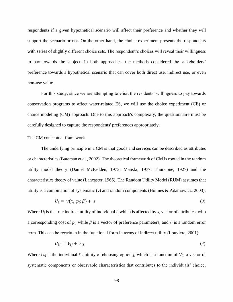
98
respondents if a given hypothetical scenario will affect their preference and whether they will
support the scenario or not. On the other hand, the choice experiment presents the respondents
with series of slightly different choice sets. The respondent’s choices will reveal their willingness
to pay towards the subject. In both approaches, the methods considered the stakeholders’
preference towards a hypothetical scenario that can cover both direct use, indirect use, or even
non-use value.
For this study, since we are attempting to elicit the residents’ willingness to pay towards
conservation programs to affect water-related ES, we will use the choice experiment (CE) or
choice modeling (CM) approach. Due to this approach's complexity, the questionnaire must be
carefully designed to capture the respondents' preferences appropriately.
The CM conceptual framework
The underlying principle in a CM is that goods and services can be described as attributes
or characteristics (Bateman et al., 2002). The theoretical framework of CM is rooted in the random
utility model theory (Daniel McFadden, 1973; Manski, 1977; Thurstone, 1927) and the
characteristics theory of value (Lancaster, 1966). The Random Utility Model (RUM) assumes that
utility is a combination of systematic (v) and random components (Holmes & Adamowicz, 2003):
𝑈𝑖 = 𝑣(𝑥𝑖, 𝑝𝑖; 𝛽) + 𝜀𝑖 (3)
Where Ui is the true indirect utility of individual i, which is affected by xi vector of attributes, with
a corresponding cost of pi, while β is a vector of preference parameters, and εi is a random error
term. This can be rewritten in the functional form in terms of indirect utility (Louviere, 2001):
𝑈𝑖𝑗 = 𝑉𝑖𝑗 + 𝜀𝑖𝑗 (4)
Where Uij is the individual i’s utility of choosing option j, which is a function of Vij, a vector of
systematic components or observable characteristics that contributes to the individuals’ choice,
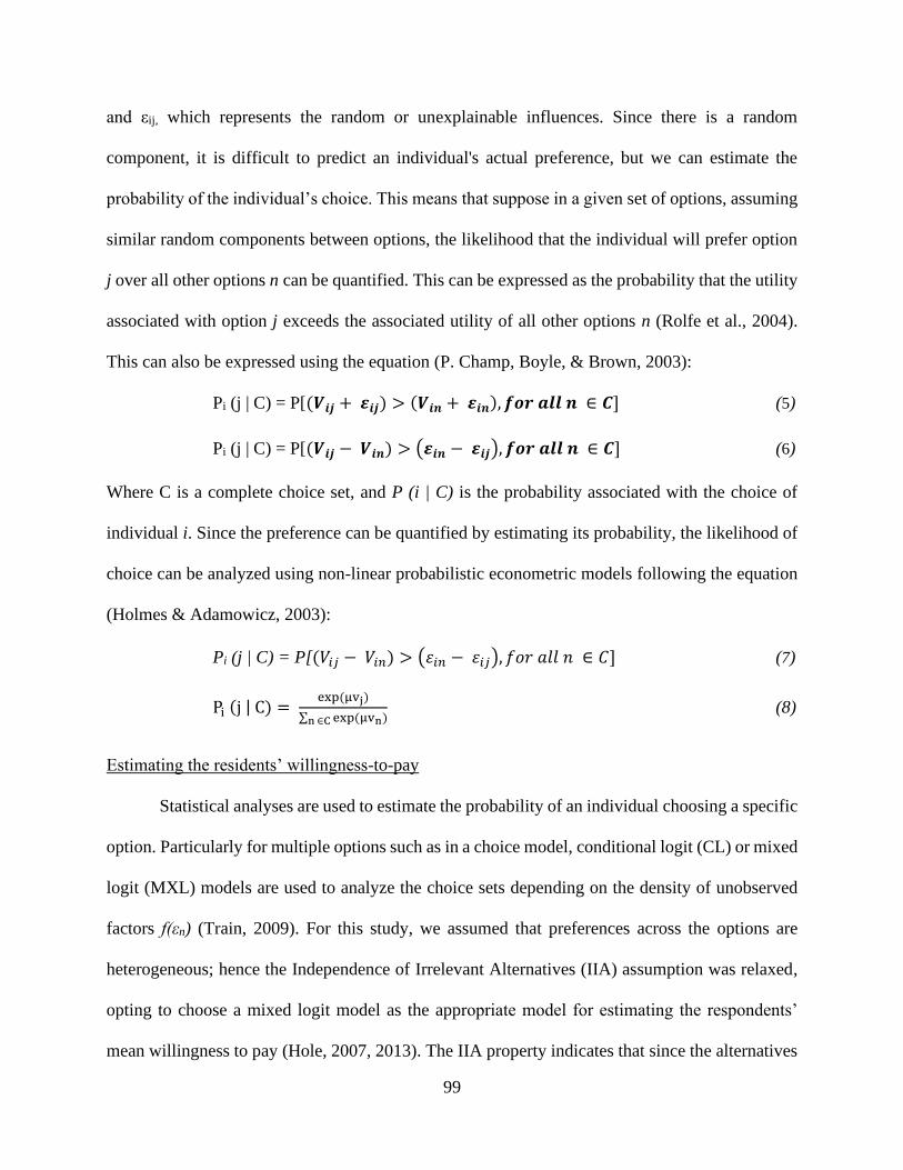
99
and εij, which represents the random or unexplainable influences. Since there is a random
component, it is difficult to predict an individual's actual preference, but we can estimate the
probability of the individual’s choice. This means that suppose in a given set of options, assuming
similar random components between options, the likelihood that the individual will prefer option
j over all other options n can be quantified. This can be expressed as the probability that the utility
associated with option j exceeds the associated utility of all other options n (Rolfe et al., 2004).
This can also be expressed using the equation (P. Champ, Boyle, & Brown, 2003):
Pi (j | C) = P[(𝑽𝒊𝒋 + 𝜺𝒊𝒋) > (𝑽𝒊𝒏 + 𝜺𝒊𝒏), 𝒇𝒐𝒓 𝒂𝒍𝒍 𝒏 ∈ 𝑪] (5)
Pi (j | C) = P[(𝑽𝒊𝒋 − 𝑽𝒊𝒏) > (𝜺𝒊𝒏 − 𝜺𝒊𝒋), 𝒇𝒐𝒓 𝒂𝒍𝒍 𝒏 ∈ 𝑪] (6)
Where C is a complete choice set, and P (i | C) is the probability associated with the choice of
individual i. Since the preference can be quantified by estimating its probability, the likelihood of
choice can be analyzed using non-linear probabilistic econometric models following the equation
(Holmes & Adamowicz, 2003):
Pi (j | C) = P[(𝑉𝑖𝑗 − 𝑉𝑖𝑛) > (𝜀𝑖𝑛 − 𝜀𝑖𝑗), 𝑓𝑜𝑟 𝑎𝑙𝑙 𝑛 ∈ 𝐶] (7)
Pi (j | C) = exp(μvj)
∑ exp(μvn)n ∈C (8)
Estimating the residents’ willingness-to-pay
Statistical analyses are used to estimate the probability of an individual choosing a specific
option. Particularly for multiple options such as in a choice model, conditional logit (CL) or mixed
logit (MXL) models are used to analyze the choice sets depending on the density of unobserved
factors f(εn) (Train, 2009). For this study, we assumed that preferences across the options are
heterogeneous; hence the Independence of Irrelevant Alternatives (IIA) assumption was relaxed,
opting to choose a mixed logit model as the appropriate model for estimating the respondents’
mean willingness to pay (Hole, 2007, 2013). The IIA property indicates that since the alternatives
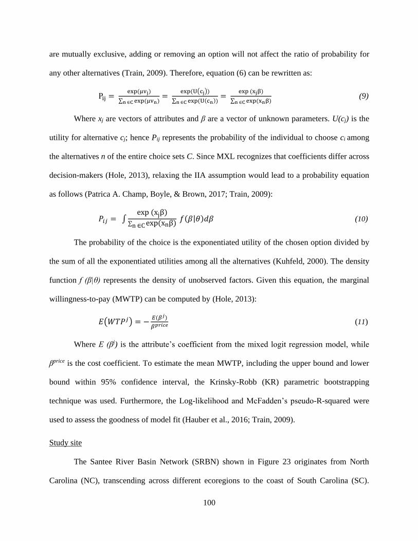
100
are mutually exclusive, adding or removing an option will not affect the ratio of probability for
any other alternatives (Train, 2009). Therefore, equation (6) can be rewritten as:
Pij = exp(μvj)
∑ exp(μvn)n ∈C=
exp(U(cj))
∑ exp(U(cn))n ∈C=
exp (xjβ)
∑ exp(xnβ)n ∈C (9)
Where xj are vectors of attributes and β are a vector of unknown parameters. U(cj) is the
utility for alternative cj; hence Pij represents the probability of the individual to choose ci among
the alternatives n of the entire choice sets C. Since MXL recognizes that coefficients differ across
decision-makers (Hole, 2013), relaxing the IIA assumption would lead to a probability equation
as follows (Patrica A. Champ, Boyle, & Brown, 2017; Train, 2009):
𝑃𝑖𝑗 = ∫exp (xjβ)
∑ exp(xnβ)n ∈C 𝑓(𝛽|𝜃)𝑑𝛽 (10)
The probability of the choice is the exponentiated utility of the chosen option divided by
the sum of all the exponentiated utilities among all the alternatives (Kuhfeld, 2000). The density
function f (β|θ) represents the density of unobserved factors. Given this equation, the marginal
willingness-to-pay (MWTP) can be computed by (Hole, 2013):
𝐸(𝑊𝑇𝑃𝑗) = −𝐸(𝛽𝑗)
𝛽𝑝𝑟𝑖𝑐𝑒 (11)
Where E (βj) is the attribute’s coefficient from the mixed logit regression model, while
βprice is the cost coefficient. To estimate the mean MWTP, including the upper bound and lower
bound within 95% confidence interval, the Krinsky-Robb (KR) parametric bootstrapping
technique was used. Furthermore, the Log-likelihood and McFadden’s pseudo-R-squared were
used to assess the goodness of model fit (Hauber et al., 2016; Train, 2009).
Study site
The Santee River Basin Network (SRBN) shown in Figure 23 originates from North
Carolina (NC), transcending across different ecoregions to the coast of South Carolina (SC).
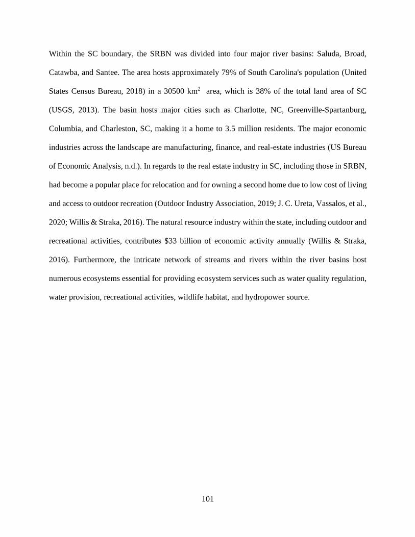
101
Within the SC boundary, the SRBN was divided into four major river basins: Saluda, Broad,
Catawba, and Santee. The area hosts approximately 79% of South Carolina's population (United
States Census Bureau, 2018) in a 30500 km2 area, which is 38% of the total land area of SC
(USGS, 2013). The basin hosts major cities such as Charlotte, NC, Greenville-Spartanburg,
Columbia, and Charleston, SC, making it a home to 3.5 million residents. The major economic
industries across the landscape are manufacturing, finance, and real-estate industries (US Bureau
of Economic Analysis, n.d.). In regards to the real estate industry in SC, including those in SRBN,
had become a popular place for relocation and for owning a second home due to low cost of living
and access to outdoor recreation (Outdoor Industry Association, 2019; J. C. Ureta, Vassalos, et al.,
2020; Willis & Straka, 2016). The natural resource industry within the state, including outdoor and
recreational activities, contributes $33 billion of economic activity annually (Willis & Straka,
2016). Furthermore, the intricate network of streams and rivers within the river basins host
numerous ecosystems essential for providing ecosystem services such as water quality regulation,
water provision, recreational activities, wildlife habitat, and hydropower source.
102
Figure 23 The Santee River Basin Network in South Carolina, USA
Data collection
To elicit the residents’ WTP, we surveyed 1500 residents across the SRBN using the
Qualtrics online platform in 2019. Since most residents of SC (79%) are connected to the internet
(U.S. Department of Commerce Census Bureau, 2019), utilizing the online platform became an
efficient manner of collecting the residents’ responses. Simple random sampling (SRS) was used
to determine the selected respondents from a list of residential emails available in the Qualtrics
database.
The survey instrument (Appendix L) was divided into six sections: 1) knowledge,
awareness, and perception of concepts; 2) infographics on basic concepts of ecosystems,
ecosystem services, and the current land cover situation in SRBN; 3) valuation scenario and
103
assumptions; 4) choice model elicitation; 5) institutional design; and 6) demographic
characteristics.
We included screener questions to ensure that the respondents are at least 18 years of age,
the household's financial decision-maker, and that their household has its water bill account. The
latter screener question was necessary to represent better the survey's payment vehicle. To ensure
a proportional representation of the population from different counties, we estimated the number
of samples to be collected per county based on its total population.
The 1500 respondents were divided into two groups representing the two types of
intervention: a farm-based intervention through cover crop planting and a tree-based intervention
through agroforestry farming. The split was necessary since each intervention has a different
magnitude of effects for the target ES attributes.
To limit the respondents’ strategic and hypothetical biases in answering the questions, we
used cheap talk statements to remind them that, although the proposition is hypothetical, they
should decide as if they are choosing for an actual policy (Patricia A Champ, Moore, & Bishop,
2009; Cummings & Taylor, 1999; Murphy, Stevens, & Weatherhead, 2005). Furthermore, when
answering the questions, they should only think about their household and not how others will be
affected.
Survey design
Knowledge, Awareness, and Perception
The first section asked questions about the respondents’ knowledge and familiarity with
ecosystems and ecosystem services concepts. This establishes a baseline of how much the
respondents know about the ecological terminology and its relation to their well-being.

104
Furthermore, it also elicits their position on some potential actionable issues relevant to
implementing these programs.
Concepts infographics and the status quo
The second section provided them with information about the basic concepts and
terminologies. After the first section, this was critically placed to correct potential misconceptions
of terminologies coming from their baseline knowledge. We also provided them information about
the current land use situation, the approximate amount of ecosystem services a watershed provides,
and how these could change in the next ten years if no conservation intervention is conducted. This
was presented as the status quo or the “business-as-usual (BAU)” scenario. We also introduced
information about cover cropping and agroforestry as some of the potential sustainable
interventions that can address the possible effects of the BAU on the ecosystems and its services.
This section allowed the respondents to have a similar understanding of the study's concepts and
primary focus. We used a combination of video clips, images, and narratives for a more interactive
information session.
Valuation scenario and assumptions
Considering the information provided in the first and second sections, the third section
presented the study's primary objective for eliciting the residents’ value for ecosystem service
improvement. We presented them with a hypothetical policy for supporting conservation programs
wherein a certain fee will be collected from the residents in 5 years through an additional charge
to their household’s monthly water bill. When answering, we asked them to consider:
a) that the money collected will be directly going to a trust fund for the river-basin
conservation;
105
b) that the overall collected funds will be solely spent for the implementation of programs
toward conservation programs and improvement of ecosystem services
c) to treat the amount that they will pay for as the amount they are willing to spend to
improve the ecosystem services.
These specifications were necessary to simulate the institutional arrangement of a PES
(Forest Trends et al., 2008; Thompson, 2018). Furthermore, we also asked them to consider that
the amount they will be paying is an addition to their current water bill. This point was emphasized
to make sure that they will be considering their constraint in their decisions. We also told them to
assume that the policy will only be implemented if the majority will be willing to participate;
however, it will apply to all residents once implemented.
Choice sets, attributes targeting, and elicitation
The fourth section of the questionnaire elicited the respondent’s preference by presenting
sets of choices with varying attributes and the choice set’s corresponding price. The choice sets
that the respondents will get depends on what sampling group they belong to, that is, the type of
intervention to be implemented across the landscape. The first one (Figure 24) simulates the
potential effect on the ecosystem services given that a crop-based sustainable practice is
implemented, particularly by planting cover crops in idle cropland. The other group (Figure 25)
simulates a tree-based sustainable practice, particularly by developing an agroforestry farm.

106
Figure 24 Sample choice set with cover crop as the intervention
Figure 25 Sample choice set with agroforestry as the intervention
While the two groups have similar ES attributes being valued, the magnitude of each
intervention's effect differs from each other. The percent change impact of the intervention on the
ES attribute was quantified using the Integrated Valuation of Ecosystem Services and Tradeoffs
(InVEST) model. Specifically, we quantified how much the ES will change for the next ten years

107
if either intervention is implemented across the landscape. We focused on the water-related ES,
particularly sediment retention capacity, potential water yield, and wildlife habitat improvement,
following the stakeholders’ prioritization preference of ecosystem services in SRBN (J. C. Ureta,
Vassalos, et al., 2020). We followed the methodology of Ureta et al. (2020) for quantifying the
sediment retention capacity and potential water yield (J. C. Ureta, Clay, et al., 2020) while
consulting wildlife experts for estimating the likely change in wildlife habitat coming from either
intervention.
To simplify the quantification of the ES effect from both interventions, we assumed that
they are mutually exclusive. Therefore, the effects in the choice set will apply solely from the
specific intervention as presented and not a combination of interventions.
The quantification results suggest that suppose if we continue as business as usual (status
quo) with no conservation measure implemented while urbanization continues to grow by 2030;
the amount of water being contributed to the stream will increase by 4%, while the amount of
sediments exported to the stream will also increase by 3% which is deterrent to the water quality.
Furthermore, a potential loss of 5-10% in habitat for bobwhite quails, deer, and songbirds may
also occur. However, with conservation programs or sustainable practices, the effect on the ES
attributes changes. Particularly if the intervention is by using cover crops, it is expected to increase
water supply by 1% while also improving water quality by 1.4%. At the very least, this intervention
maintains or minimizes the loss of the wildlife habitat or improves some occurrence of wildlife.
On the other hand, if the intervention implemented is by agroforestry farming, it is expected to
increase the water supply volume across the landscape by 3% while also improving the water
quality by reducing sediments exported by 5%. Furthermore, this intervention also enhances
wildlife habitat through the increased frequency of bobwhite quails, deer, and songbirds by 5-10%.
108
Given the quantification of ecosystem services, each option comprised four attributes (3
ecosystem services and a price of the bundle) with two levels each. We used the JMP software
(SAS Institute Inc., 2019) to randomize the attribute levels to form the optimal choice sets. With a
D-efficiency of 91% for the cover crop sampling group and 90% for the agroforestry sampling
group, the JMP generated 12 choice sets in total for both sampling groups with two options per
choice set. The two levels per choice set become Options 1 and 2, while the status quo became
Option 3. Overall, each respondent was presented with four choice sets, further subdividing the
sampling group into three clusters to distribute the 12 choice sets among the respondents evenly.
Institutional arrangement
The fifth section of the questionnaire elicits the respondents preferred institutional
arrangement should a PES be established. At this point, respondents were asked about their
recommendation on the best payment vehicle to collect the PES funds. Also, they were asked about
the possible type of institution that should be trusted to manage the funds and lead the PES
program. This question is critical in establishing a PES as it provides information on the possible
institutional arrangement that the public would vouch for. The institution with the strongest
support from the public is critical for successfully implementing a PES (Goldman et al., 2007;
Thompson, 2018).
Respondent profile
Finally, the sixth part of the questionnaire elicited the respondents’ profile. In decision-
making exercises or social science surveys, demographic variables show that respondents’
characteristics may or may not have a connection towards their decision-making criteria; hence it
can be used as exogenous covariates in the analysis (Abdul-Wahab & Abdo, 2010; Mangiafico et
al., 2012; Muhammad Nauman Sadiq et al., 2014; Vilčeková & Sabo, 2013). Furthermore, socio-
109
economic characteristics are typical factors used in evaluating decision-making as this constitutes
constraint attributes to respondents. This is typical of valuation and stakeholder involvement
studies (Mangiafico et al., 2012; Marsh, 2014; Seriño et al., 2017; Small et al., 2017; Soley et al.,
2019; J.C.P. Ureta et al., 2016).
Results and discussion
The respondents' socio-demographic characteristics from both sampling groups divided
into the three regions of SRBN as Upstate, Midland, and Lowcountry & Coastal) are reported in
Table 11.
Demographic characteristics
The average age of respondents from both the sampling group and across the region is
relatively similar, ranging at around 48 – 49 years of age for the agroforestry group, while 48 – 51
for the cover crop group. Similarly, the average household size is three across the sampling groups,
which is comparable to the national and state statistics (United States Census Bureau, 2018). The
average years that respondents stayed in SC ranged from 25 – 29 years for the agroforestry group,
while 22 – 31 years for the cover crops group. Furthermore, most of the respondents in both groups
own the house they are currently living in.
In terms of social characteristics, while most of the respondents across the group are female
(60% to 72% across the clusters), a substantial percentage of males participated in the survey (28%
to 40%). In terms of ethnicity, most of the respondents identified themselves as white or Caucasian,
76% - 89%, which is slightly higher than the state’s overall average of 67% of the total population
(United States Census Bureau, 2019a). Furthermore, the number of respondents that has a
bachelor’s degree or higher (46% to 57% in the agroforestry group, while 43% to 51% in the cover
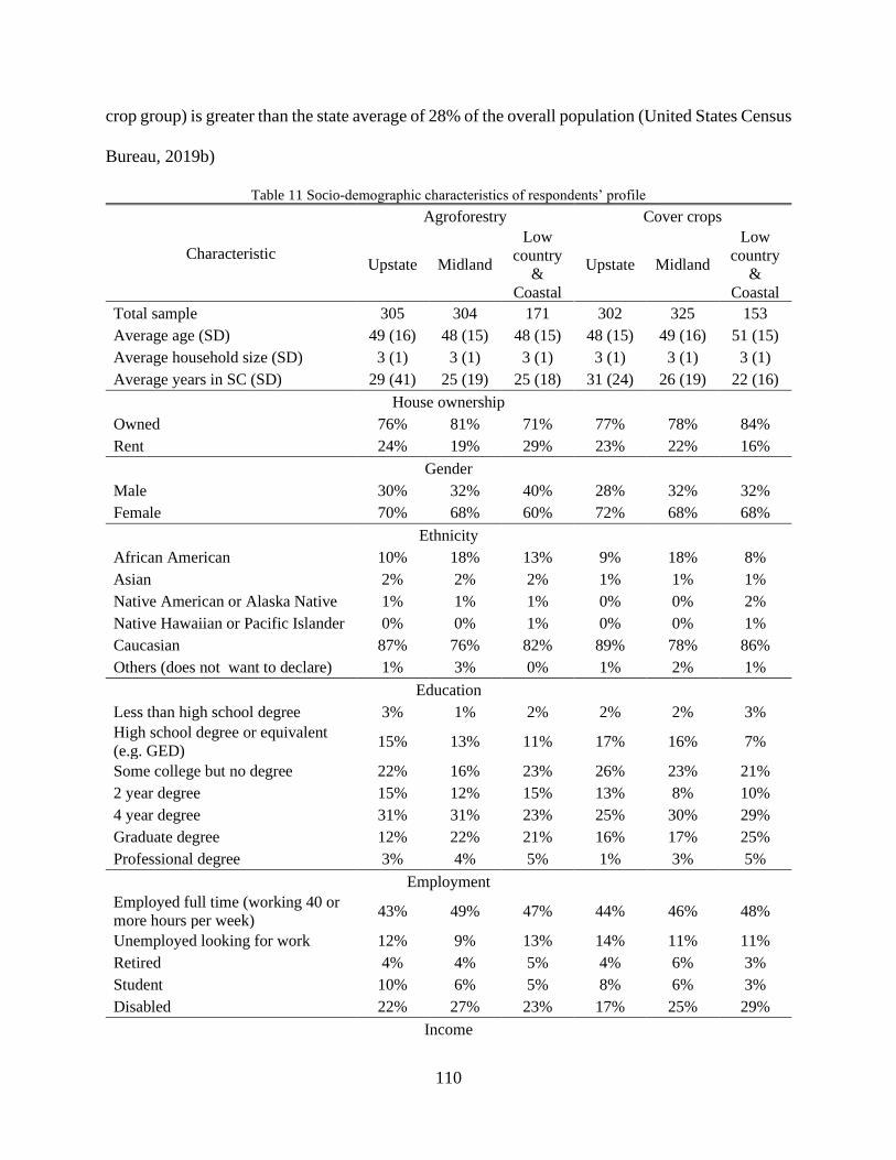
110
crop group) is greater than the state average of 28% of the overall population (United States Census
Bureau, 2019b)
Table 11 Socio-demographic characteristics of respondents’ profile
Characteristic
Agroforestry Cover crops
Upstate Midland
Low
country
&
Coastal
Upstate Midland
Low
country
&
Coastal
Total sample 305 304 171 302 325 153
Average age (SD) 49 (16) 48 (15) 48 (15) 48 (15) 49 (16) 51 (15)
Average household size (SD) 3 (1) 3 (1) 3 (1) 3 (1) 3 (1) 3 (1)
Average years in SC (SD) 29 (41) 25 (19) 25 (18) 31 (24) 26 (19) 22 (16)
House ownership
Owned 76% 81% 71% 77% 78% 84%
Rent 24% 19% 29% 23% 22% 16%
Gender
Male 30% 32% 40% 28% 32% 32%
Female 70% 68% 60% 72% 68% 68%
Ethnicity
African American 10% 18% 13% 9% 18% 8%
Asian 2% 2% 2% 1% 1% 1%
Native American or Alaska Native 1% 1% 1% 0% 0% 2%
Native Hawaiian or Pacific Islander 0% 0% 1% 0% 0% 1%
Caucasian 87% 76% 82% 89% 78% 86%
Others (does not want to declare) 1% 3% 0% 1% 2% 1%
Education
Less than high school degree 3% 1% 2% 2% 2% 3%
High school degree or equivalent
(e.g. GED) 15% 13% 11% 17% 16% 7%
Some college but no degree 22% 16% 23% 26% 23% 21%
2 year degree 15% 12% 15% 13% 8% 10%
4 year degree 31% 31% 23% 25% 30% 29%
Graduate degree 12% 22% 21% 16% 17% 25%
Professional degree 3% 4% 5% 1% 3% 5%
Employment
Employed full time (working 40 or
more hours per week) 43% 49% 47% 44% 46% 48%
Unemployed looking for work 12% 9% 13% 14% 11% 11%
Retired 4% 4% 5% 4% 6% 3%
Student 10% 6% 5% 8% 6% 3%
Disabled 22% 27% 23% 17% 25% 29%
Income
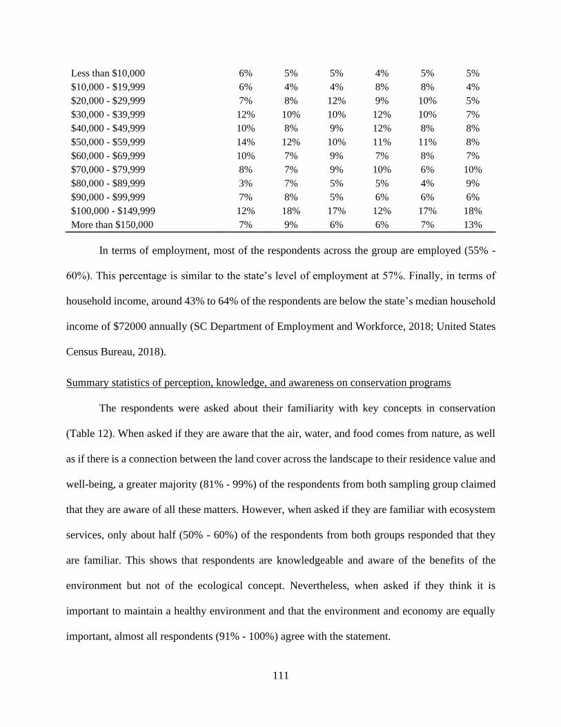
111
Less than $10,000 6% 5% 5% 4% 5% 5%
$10,000 - $19,999 6% 4% 4% 8% 8% 4%
$20,000 - $29,999 7% 8% 12% 9% 10% 5%
$30,000 - $39,999 12% 10% 10% 12% 10% 7%
$40,000 - $49,999 10% 8% 9% 12% 8% 8%
$50,000 - $59,999 14% 12% 10% 11% 11% 8%
$60,000 - $69,999 10% 7% 9% 7% 8% 7%
$70,000 - $79,999 8% 7% 9% 10% 6% 10%
$80,000 - $89,999 3% 7% 5% 5% 4% 9%
$90,000 - $99,999 7% 8% 5% 6% 6% 6%
$100,000 - $149,999 12% 18% 17% 12% 17% 18%
More than $150,000 7% 9% 6% 6% 7% 13%
In terms of employment, most of the respondents across the group are employed (55% -
60%). This percentage is similar to the state’s level of employment at 57%. Finally, in terms of
household income, around 43% to 64% of the respondents are below the state’s median household
income of $72000 annually (SC Department of Employment and Workforce, 2018; United States
Census Bureau, 2018).
Summary statistics of perception, knowledge, and awareness on conservation programs
The respondents were asked about their familiarity with key concepts in conservation
(Table 12). When asked if they are aware that the air, water, and food comes from nature, as well
as if there is a connection between the land cover across the landscape to their residence value and
well-being, a greater majority (81% - 99%) of the respondents from both sampling group claimed
that they are aware of all these matters. However, when asked if they are familiar with ecosystem
services, only about half (50% - 60%) of the respondents from both groups responded that they
are familiar. This shows that respondents are knowledgeable and aware of the benefits of the
environment but not of the ecological concept. Nevertheless, when asked if they think it is
important to maintain a healthy environment and that the environment and economy are equally
important, almost all respondents (91% - 100%) agree with the statement.
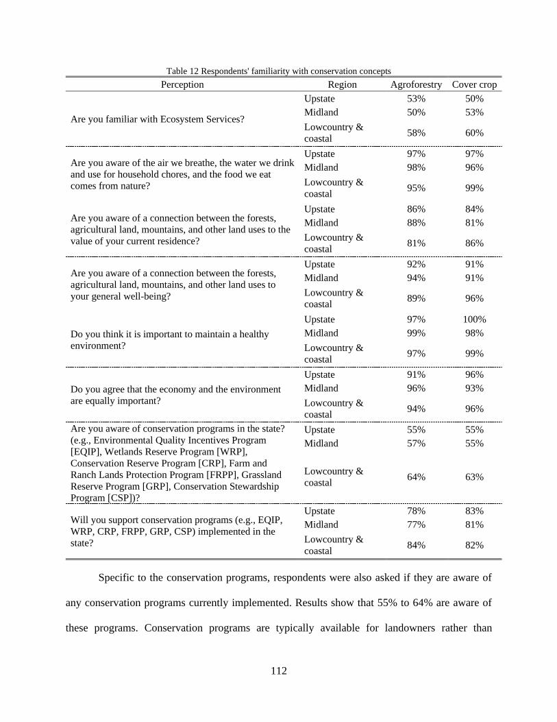
112
Table 12 Respondents' familiarity with conservation concepts
Perception Region Agroforestry Cover crop
Are you familiar with Ecosystem Services?
Upstate 53% 50%
Midland 50% 53%
Lowcountry &
coastal 58% 60%
Are you aware of the air we breathe, the water we drink
and use for household chores, and the food we eat
comes from nature?
Upstate 97% 97%
Midland 98% 96%
Lowcountry &
coastal 95% 99%
Are you aware of a connection between the forests,
agricultural land, mountains, and other land uses to the
value of your current residence?
Upstate 86% 84%
Midland 88% 81%
Lowcountry &
coastal 81% 86%
Are you aware of a connection between the forests,
agricultural land, mountains, and other land uses to
your general well-being?
Upstate 92% 91%
Midland 94% 91%
Lowcountry &
coastal 89% 96%
Do you think it is important to maintain a healthy
environment?
Upstate 97% 100%
Midland 99% 98%
Lowcountry &
coastal 97% 99%
Do you agree that the economy and the environment
are equally important?
Upstate 91% 96%
Midland 96% 93%
Lowcountry &
coastal 94% 96%
Are you aware of conservation programs in the state?
(e.g., Environmental Quality Incentives Program
[EQIP], Wetlands Reserve Program [WRP],
Conservation Reserve Program [CRP], Farm and
Ranch Lands Protection Program [FRPP], Grassland
Reserve Program [GRP], Conservation Stewardship
Program [CSP])?
Upstate 55% 55%
Midland 57% 55%
Lowcountry &
coastal 64% 63%
Will you support conservation programs (e.g., EQIP,
WRP, CRP, FRPP, GRP, CSP) implemented in the
state?
Upstate 78% 83%
Midland 77% 81%
Lowcountry &
coastal 84% 82%
Specific to the conservation programs, respondents were also asked if they are aware of
any conservation programs currently implemented. Results show that 55% to 64% are aware of
these programs. Conservation programs are typically available for landowners rather than
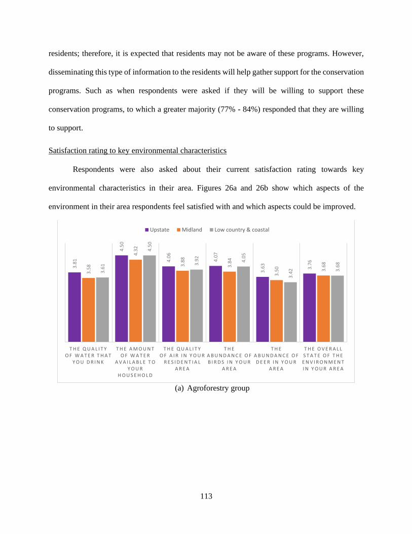
113
residents; therefore, it is expected that residents may not be aware of these programs. However,
disseminating this type of information to the residents will help gather support for the conservation
programs. Such as when respondents were asked if they will be willing to support these
conservation programs, to which a greater majority (77% - 84%) responded that they are willing
to support.
Satisfaction rating to key environmental characteristics
Respondents were also asked about their current satisfaction rating towards key
environmental characteristics in their area. Figures 26a and 26b show which aspects of the
environment in their area respondents feel satisfied with and which aspects could be improved.
(a) Agroforestry group
3.8
1
4.5
0
4.0
6
4.0
7
3.6
3
3.7
6
3.5
8
4.3
2
3.8
8
3.8
4
3.5
0 3.6
8
3.6
1
4.5
0
3.9
2
4.0
5
3.4
2 3.6
8
T H E Q U A L I T Y O F W A T E R T H A T
Y O U D R I N K
T H E A M O U N T O F W A T E R
A V A I L A B L E T O Y O U R
H O U S E H O L D
T H E Q U A L I T Y O F A I R I N Y O U R
R E S I D E N T I A L A R E A
T H E A B U N D A N C E O F B I R D S I N Y O U R
A R E A
T H E A B U N D A N C E O F D E E R I N Y O U R
A R E A
T H E O V E R A L L S T A T E O F T H E E N V I R O N M E N T I N Y O U R A R E A
Upstate Midland Low country & coastal

114
(b) Cover crop group
Figure 26 Median satisfaction rating of respondents to key environmental characteristics in their area
Overall, results show a remarkably similar satisfaction rating in both groups with few
differences by region (Appendix K). Figure 26 shows that respondents have the highest median
satisfaction rating towards the amount of water available to the household. The rating between the
regions also shows the same pattern where Lowcountry and coastal areas have the highest median
satisfaction rate for water supply (4.50 for agroforestry group and 4.53 from cover crop group),
followed by Upstate residents (4.50 and 4.48), and lastly by the Midland residents (4.32 and 4.25).
In general, this could imply that there is no issue with the water supply within SRBN. The results
coincide with the potential water yield quantification study of Ureta et al. (2020), where
Lowcountry and coastal areas showed to accumulate water due to convergence of rivers and
presence of low lying areas, while upstate regions are where the headwaters of watershed can be
found (J. C. Ureta, Clay, et al., 2020).
3.6
5
4.4
8
3.8
7
3.9
9
3.5
9
3.6
6
3.4
9
4.2
5
3.8
3
3.9
0
3.6
2
3.6
53.9
3
4.5
3
4.0
7
3.9
3
3.5
5
3.6
8
T H E Q U A L I T Y O F W A T E R T H A T
Y O U D R I N K
T H E A M O U N T O F W A T E R
A V A I L A B L E T O Y O U R
H O U S E H O L D
T H E Q U A L I T Y O F A I R I N Y O U R R E S I D E N T I A L
A R E A
T H E A B U N D A N C E O F B I R D S I N Y O U R
A R E A
T H E A B U N D A N C E O F D E E R I N Y O U R
A R E A
T H E O V E R A L L S T A T E O F T H E E N V I R O N M E N T I N Y O U R A R E A
Upstate Midland Low country & coastal
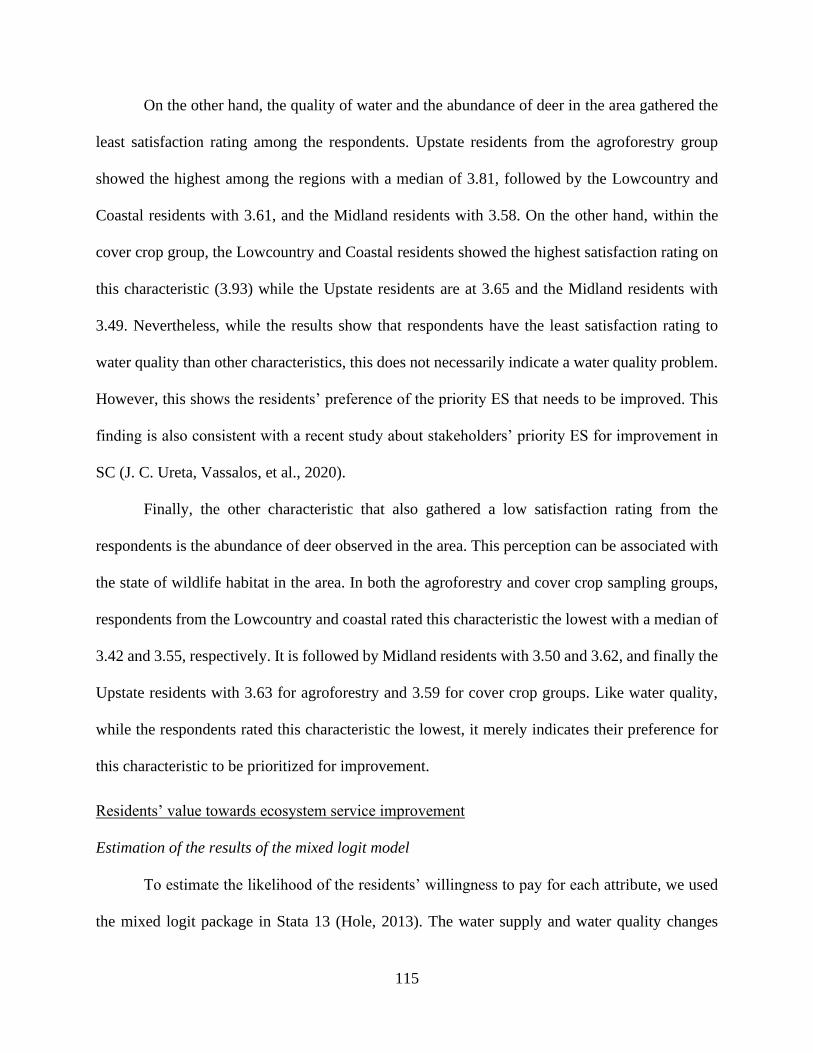
115
On the other hand, the quality of water and the abundance of deer in the area gathered the
least satisfaction rating among the respondents. Upstate residents from the agroforestry group
showed the highest among the regions with a median of 3.81, followed by the Lowcountry and
Coastal residents with 3.61, and the Midland residents with 3.58. On the other hand, within the
cover crop group, the Lowcountry and Coastal residents showed the highest satisfaction rating on
this characteristic (3.93) while the Upstate residents are at 3.65 and the Midland residents with
3.49. Nevertheless, while the results show that respondents have the least satisfaction rating to
water quality than other characteristics, this does not necessarily indicate a water quality problem.
However, this shows the residents’ preference of the priority ES that needs to be improved. This
finding is also consistent with a recent study about stakeholders’ priority ES for improvement in
SC (J. C. Ureta, Vassalos, et al., 2020).
Finally, the other characteristic that also gathered a low satisfaction rating from the
respondents is the abundance of deer observed in the area. This perception can be associated with
the state of wildlife habitat in the area. In both the agroforestry and cover crop sampling groups,
respondents from the Lowcountry and coastal rated this characteristic the lowest with a median of
3.42 and 3.55, respectively. It is followed by Midland residents with 3.50 and 3.62, and finally the
Upstate residents with 3.63 for agroforestry and 3.59 for cover crop groups. Like water quality,
while the respondents rated this characteristic the lowest, it merely indicates their preference for
this characteristic to be prioritized for improvement.
Residents’ value towards ecosystem service improvement
Estimation of the results of the mixed logit model
To estimate the likelihood of the residents’ willingness to pay for each attribute, we used
the mixed logit package in Stata 13 (Hole, 2013). The water supply and water quality changes
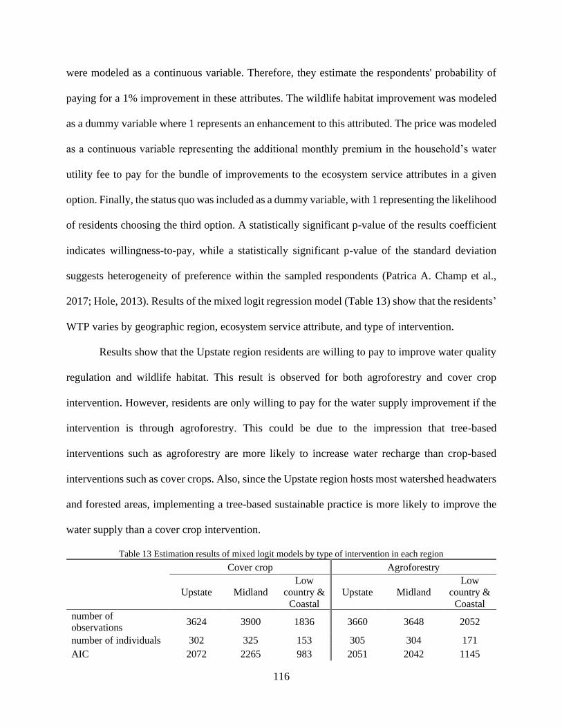
116
were modeled as a continuous variable. Therefore, they estimate the respondents' probability of
paying for a 1% improvement in these attributes. The wildlife habitat improvement was modeled
as a dummy variable where 1 represents an enhancement to this attributed. The price was modeled
as a continuous variable representing the additional monthly premium in the household’s water
utility fee to pay for the bundle of improvements to the ecosystem service attributes in a given
option. Finally, the status quo was included as a dummy variable, with 1 representing the likelihood
of residents choosing the third option. A statistically significant p-value of the results coefficient
indicates willingness-to-pay, while a statistically significant p-value of the standard deviation
suggests heterogeneity of preference within the sampled respondents (Patrica A. Champ et al.,
2017; Hole, 2013). Results of the mixed logit regression model (Table 13) show that the residents’
WTP varies by geographic region, ecosystem service attribute, and type of intervention.
Results show that the Upstate region residents are willing to pay to improve water quality
regulation and wildlife habitat. This result is observed for both agroforestry and cover crop
intervention. However, residents are only willing to pay for the water supply improvement if the
intervention is through agroforestry. This could be due to the impression that tree-based
interventions such as agroforestry are more likely to increase water recharge than crop-based
interventions such as cover crops. Also, since the Upstate region hosts most watershed headwaters
and forested areas, implementing a tree-based sustainable practice is more likely to improve the
water supply than a cover crop intervention.
Table 13 Estimation results of mixed logit models by type of intervention in each region Cover crop Agroforestry
Upstate Midland
Low
country &
Coastal
Upstate Midland
Low
country &
Coastal
number of
observations 3624 3900 1836 3660 3648 2052
number of individuals 302 325 153 305 304 171
AIC 2072 2265 983 2051 2042 1145
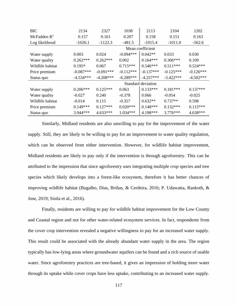
117
BIC 2134 2327 1038 2113 2104 1202
McFadden R2 0.157 0.161 0.207 0.158 0.151 0.163
Log likelihood -1026.1 -1122.3 -481.5 -1015.4 -1011.0 -562.6 Mean coefficient
Water supply 0.003 0.024 -0.094*** 0.042** 0.033 0.030
Water quality 0.262*** 0.262*** 0.002 0.164*** 0.306*** 0.109
Wildlife habitat 0.195* 0.067 0.715*** 0.546*** 0.511*** 0.524***
Price premium -0.087*** -0.091*** -0.112*** -0.137*** -0.125*** -0.126***
Status quo -4.534*** -4.208*** -6.289*** -4.257*** -3.422*** -4.502*** Standard deviation
Water supply 0.206*** 0.125*** 0.063 0.133*** 0.181*** 0.137***
Water quality -0.027 0.240 -0.378 0.066 -0.054 -0.025
Wildlife habitat -0.014 0.115 -0.357 0.632** 0.737** 0.598
Price premium 0.149*** 0.127*** 0.020*** 0.148*** 0.132*** 0.115***
Status quo 3.944*** 4.633*** 1.034*** 4.198*** 3.776*** 4.638***
Similarly, Midland residents are also unwilling to pay for the improvement of the water
supply. Still, they are likely to be willing to pay for an improvement to water quality regulation,
which can be observed from either intervention. However, for wildlife habitat improvement,
Midland residents are likely to pay only if the intervention is through agroforestry. This can be
attributed to the impression that since agroforestry uses integrating multiple crop species and tree
species which likely develops into a forest-like ecosystem, therefore it has better chances of
improving wildlife habitat (Bugalho, Dias, Briñas, & Cerdeira, 2016; P. Udawatta, Rankoth, &
Jose, 2019; Sistla et al., 2016).
Finally, residents are willing to pay for wildlife habitat improvement for the Low County
and Coastal region and not for other water-related ecosystem services. In fact, respondents from
the cover crop intervention revealed a negative willingness to pay for an increased water supply.
This result could be associated with the already abundant water supply in the area. The region
typically has low-lying areas where groundwater aquifers can be found and a rich source of usable
water. Since agroforestry practices are tree-based, it gives an impression of holding more water
through its uptake while cover crops have less uptake, contributing to an increased water supply.

118
Therefore, with the abundance of water and occurrence of flooding incidents in these regions,
residents could have an impression that they already have an excessive amount of water, to the
point that it is already damaging rather than beneficial. The water quality is less of a concern in
this region since the Lowcountry and Coastal areas have a relatively high satisfaction rating for
this attribute than other regions (Figure 26).
Computing for the marginal willingness to pay
Using the Krinsky-Robb (KR) parametric bootstrapping, the marginal willingness-to-pay
(MWTP) was computed for statistically significant attributes and a 95% confidence interval by
region and by ES (Figure 27).
In terms of water supply, Upstate residents’ WTP is estimated to be around $0.31, mainly
only if the intervention is agroforestry. On the other hand, the Lowcountry and Coastal residents
revealed a negative WTP amounting to -$0.84, representing the amount they should be
compensated for a percent increase in the volume of water they are currently receiving.
Upstate residents are willing to pay $3.00 if the intervention is through the cover crop in
terms of water quality, while $1.19 if the intervention is through agroforestry. Midland residents
are willing to pay $2.86 and $2.44, respectively, while Lowcountry and Coastal residents are
unwilling to pay for this attribute. In both regions, residents’ WTP through cover crops are higher
than agroforestry. This could be associated with the popularity of the cover crop intervention
within SC. The state has been promoting cover crops as a sustainable farming practice, hence also
highlighting its benefits. On the other hand, there are still minimal resources and information for
agroforestry, and very few farmers and landowners have adopted this practice.
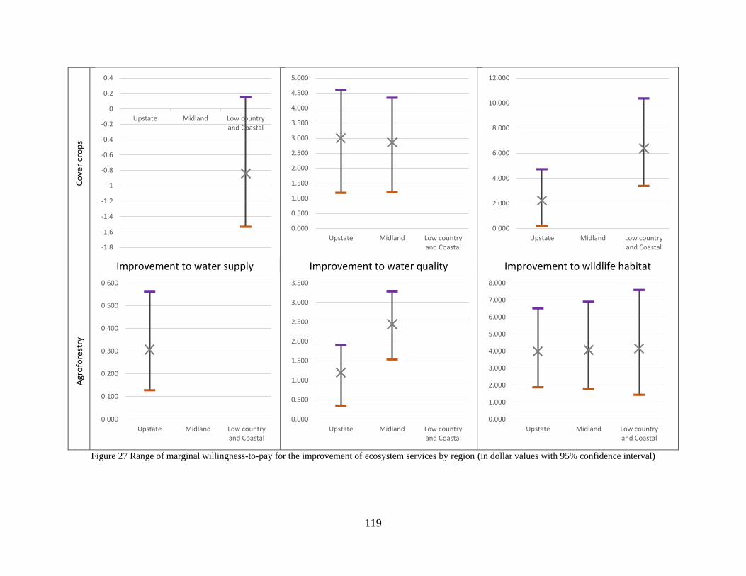
119
Co
ver
cro
ps
Improvement to water supply Improvement to water quality Improvement to wildlife habitat
Agr
ofo
rest
ry
Figure 27 Range of marginal willingness-to-pay for the improvement of ecosystem services by region (in dollar values with 95% confidence interval)
-1.8
-1.6
-1.4
-1.2
-1
-0.8
-0.6
-0.4
-0.2
0
0.2
0.4
Upstate Midland Low countryand Coastal
0.000
0.500
1.000
1.500
2.000
2.500
3.000
3.500
4.000
4.500
5.000
Upstate Midland Low countryand Coastal
0.000
2.000
4.000
6.000
8.000
10.000
12.000
Upstate Midland Low countryand Coastal
0.000
0.100
0.200
0.300
0.400
0.500
0.600
Upstate Midland Low countryand Coastal
0.000
0.500
1.000
1.500
2.000
2.500
3.000
3.500
Upstate Midland Low countryand Coastal
0.000
1.000
2.000
3.000
4.000
5.000
6.000
7.000
8.000
Upstate Midland Low countryand Coastal

120
Finally, for wildlife habitat improvement, the residents’ MWTP varies by intervention and 0
by geographic region. Upstate residents are willing to pay $2.23 if the intervention is cover crop 1
while $3.98 if agroforestry. Midland residents are unwilling to pay if the intervention is cover crop 2
but are willing to pay $4.08 for agroforestry. In both cases, the agroforestry intervention yields 3
higher WTP as compared to cover crops. This could be associated with the impression that since 4
agroforestry is more likely related to reforestation, it will have a higher likelihood of improving 5
the wildlife habitat (Bugalho et al., 2016; P. Udawatta et al., 2019; Sistla et al., 2016). However, 6
the situation is reversed for the Lowcountry and Coastal region. Residents are willing to pay $6.39 7
if the intervention is through cover crops while $4.15 for agroforestry. Lowcountry and Coastal 8
ecosystem tend to be closer to prairies and field which holds diverse species that are ecologically 9
important such as insects and birds. By implementing cover crops, keeps the areas vegetated hence 10
also maintaining the soil and species diversity across the land, which could lead to improvement 11
to wildlife habitat (de Pedro, Perera-Fernández, López-Gallego, Pérez-Marcos, & Sanchez, 2020; 12
Elhakeem et al., 2019; Shackelford, Kelsey, & Dicks, 2019). Overall, despite the differences in the 13
estimated MWTP of residents, residents have high regard for wildlife habitat improvement. This 14
is also consistent with their satisfaction rating, where characteristics relevant to wildlife habitat, 15
particularly deer sightings, have a relatively lower score than others (See Appendix M). 16
To verify the feasibility of the proposition, we also asked the respondents if they would be 17
willing to support a PES program considering the assumptions presented in the questionnaire and 18
that it could affect their household budget. Results revealed that 75% of the respondents are willing 19
to support the program. Within those who are willing to support, 44% of the respondents said their 20
reason is that they care a lot about the ecosystem services, while 55% said that they experience the 21
benefits from the ecosystem, and 32% said that they get satisfaction in contributing to a cause that 22
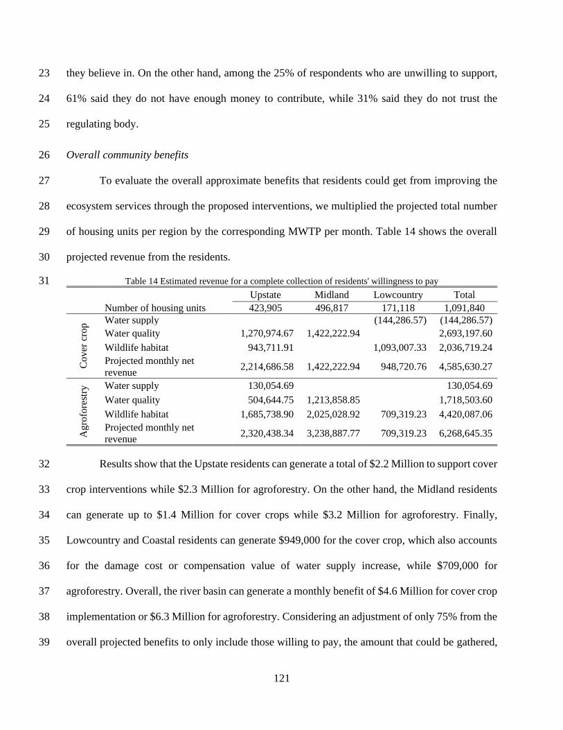
121
they believe in. On the other hand, among the 25% of respondents who are unwilling to support, 23
61% said they do not have enough money to contribute, while 31% said they do not trust the 24
regulating body. 25
Overall community benefits 26
To evaluate the overall approximate benefits that residents could get from improving the 27
ecosystem services through the proposed interventions, we multiplied the projected total number 28
of housing units per region by the corresponding MWTP per month. Table 14 shows the overall 29
projected revenue from the residents. 30
Table 14 Estimated revenue for a complete collection of residents' willingness to pay 31
Upstate Midland Lowcountry Total
Number of housing units 423,905 496,817 171,118 1,091,840
Cover
cro
p Water supply (144,286.57) (144,286.57)
Water quality 1,270,974.67 1,422,222.94 2,693,197.60
Wildlife habitat 943,711.91 1,093,007.33 2,036,719.24
Projected monthly net
revenue 2,214,686.58 1,422,222.94 948,720.76 4,585,630.27
Agro
fore
stry
Water supply 130,054.69 130,054.69
Water quality 504,644.75 1,213,858.85 1,718,503.60
Wildlife habitat 1,685,738.90 2,025,028.92 709,319.23 4,420,087.06
Projected monthly net
revenue 2,320,438.34 3,238,887.77 709,319.23 6,268,645.35
Results show that the Upstate residents can generate a total of $2.2 Million to support cover 32
crop interventions while $2.3 Million for agroforestry. On the other hand, the Midland residents 33
can generate up to $1.4 Million for cover crops while $3.2 Million for agroforestry. Finally, 34
Lowcountry and Coastal residents can generate $949,000 for the cover crop, which also accounts 35
for the damage cost or compensation value of water supply increase, while $709,000 for 36
agroforestry. Overall, the river basin can generate a monthly benefit of $4.6 Million for cover crop 37
implementation or $6.3 Million for agroforestry. Considering an adjustment of only 75% from the 38
overall projected benefits to only include those willing to pay, the amount that could be gathered, 39

122
if materialized, will be substantial for sustainable support of conservation programs. Hence, this 40
estimate reveals the economic viability of the PES program within the river basin network. 41
Preference on Institutional arrangement 42
To understand the respondents' preference regarding institutional arrangements that can 43
lead the program, we asked about their preferred payment vehicle and institutional driver for 44
conservation programs. Regarding their preferred mode of payment that should be used to collect 45
the funds for conservation programs, respondent preference is split evenly between Federal or 46
State tax payment collection and Real Estate tax collection with 38% each. While other utility bills 47
were an option, only 11% chose that type of payment vehicle. Using the Real Estate and Federal 48
or State tax system could be an advantage for PES since these are already established and auditable 49
mechanisms for collection, which mitigates one of the challenges in PES (Fauzi & Anna, 2013; 50
Thompson, 2018; Zanella et al., 2014) and hence could provide a reliable fund collection and 51
disbursement scheme. 52
On the other hand, in terms of preferred institutions that should spearhead, oversee, and 53
direct the PES framework, respondents preferred the Academia (36%), followed by non-profit 54
organizations (25%) and the State agencies (21%). This reveals that respondents have the highest 55
confidence in these institutions for driving the PES framework for the conservation program. 56
Finally, when asked if they think this type of sustainable financing program will become 57
successful and effective within the state, 43% responded “Yes” while only 5% responded “No.” 58
However, while the majority of the residents (52%) responded “Maybe,” most remarks said that 59
this program is likely to be successful as long as the stakeholders are adequately informed and that 60
there is transparency on the financial spending to ensure that the overall funds go to conservation 61
program trust fund. Furthermore, other remarks also mentioned that the program's success would 62
123
depend on the governance and institutional structure. Nevertheless, while many respondents are 63
skeptical of the program's effectiveness, most are optimistic that this sustainable financing 64
mechanism will benefit society. 65
Summary and conclusion 66
Payments for Ecosystem Services is a promising viable solution for the continuous support 67
of conservation programs and sustainable practices. However, the scheme's success is highly 68
dependent on understanding the preference of the primary key players such as the ES Sellers and 69
ES Buyers. This study mainly investigated residents' preference towards supporting conservation 70
programs and sustainable practices in a potential PES framework scheme. We also estimated the 71
residents’ value towards ecosystem services improvement, specifically to the abundance of water 72
supply, improvement on water quality regulation, and enhancement of wildlife habitat; and the 73
potential overall community benefits of the PES program. The estimation was conducted in the 74
context of proposed possible interventions of developing agroforestry or implementing cover crop 75
planting. 76
Results show that residents have a high appreciation of the benefits they get from the 77
environment, especially those with a tangible and direct impact on their well-being. However, 78
when asked about conservation concepts and programs, there was a significant decline in those 79
familiar with them. This demonstrates a knowledge gap within the public of fundamental 80
ecological concepts, which are essential for promoting and understanding the importance of 81
conservation programs and sustainable practices. Furthermore, most respondents also revealed that 82
they are unaware of different types of conservation programs. While information about 83
conservation programs and sustainable farming practices is more relevant for landowners and 84
farmers, understanding the benefits for the residents and the general public will increase the 85
124
acceptability and support for these programs. In fact, residents indicate that they are willing to pay 86
to support conservation programs and sustainable practices as long as they have knowledge and 87
information about these programs' effectiveness and success. This highlights the need to address 88
this gap by improving the education and information campaign to gather support and increase the 89
public's acceptability of the conservation programs. 90
While results indicated that residents are willing to support the conservation programs and 91
sustainable practices through the PES framework, it is also essential to estimate their value towards 92
ecosystem services improvement. Results showed that resident’s marginal willingness to pay 93
varies depending on region, the type of intervention, and the type of ecosystem service that will 94
improve. Upstate residents are willing to pay $3.00 per month for a 1% improvement on water 95
quality regulation of a cover crop planting intervention, while $1.19 if the intervention is through 96
agroforestry farming. On the other hand, Midland residents are willing to pay $2.86 to cover crop 97
intervention while $2.44 in support of an agroforestry intervention. Finally, Lowcountry and 98
Coastal residents indicated that they are unwilling to pay for a water quality improvement. In both 99
regions, Upstate and Midland, the residents’ WTP are higher for cover crop intervention than 100
agroforestry. This could be associated with the promotion of cover crops as a sustainable farming 101
practice within the state, while agroforestry farming is still exploratory. 102
Furthermore, in terms of wildlife habitat improvement, Upstate residents are willing to pay 103
$2.23 per month if cover crop planting as a sustainable practice intervention could improve the 104
wildlife habitat, while $3.98 if through agroforestry. Midland residents are unwilling to pay for 105
the cover crop as an intervention but are willing to pay $4.08 for agroforestry. The higher WTP of 106
residents for wildlife habitat improvement through agroforestry can be associated with 107
reforestation. Since agroforestry resembles reforestation, residents have the impression that 108

125
improving the forest could also improve wildlife habitat and biodiversity. However, the same 109
cannot be said for Lowcountry and Coastal region residents. The residents’ estimated WTP for 110
wildlife habitat improvement is $6.39 through cover crops intervention while $4.15 for 111
agroforestry. The difference in the preference could be due to the type of ecosystem that is within 112
this region. Since the Lowcountry and Coastal regions have many low-lying areas and most 113
ecosystems are close to prairie and agroecosystem types, the biodiversity also changes depending 114
on the kind of ecosystem. Therefore, since the cover crop is more relatable to the ecosystems in 115
this region, it is more feasible to improve the wildlife habitat of this region than agroforestry 116
farming. 117
In terms of the increase in water supply, residents are typically not willing to pay. Among 118
the regions, only Upstate residents are willing to pay $0.31 for this ecosystem service improvement 119
and only if through an agroforestry program. This could be due to the impression of agroforestry 120
which uses tree-based practices. Tree-based practices closely resemble reforestation efforts which 121
are typically linked to improvement in water recharge and water catchment. Furthermore, the 122
Upstate region hosts most headwaters, making it attractive to implement tree-based practices due 123
to the still dense surrounding forests. On the other hand, residents in the Lowcountry and Coastal 124
area revealed a negative WTP of -$0.84 through cover crop implementation. This could be due to 125
the abundance of water in the area to the point that an increased amount would become overly 126
excessive and unbeneficial. 127
Using the estimated WTP, the Upstate region's overall community benefits are estimated 128
to be around $2.2 Million per month through the cover crop sustainable farming practice while 129
$2.3 Million per month through agroforestry farming. On the other hand, the Midland region is 130
estimated to be around $1.4 Million to $3.2 Million, respectively. Lastly, the Lowcountry and 131

126
Coastal region’s community benefits are estimated at $949,000 through cover crop intervention 132
while $709,000 through agroforestry. Overall, this amounts to $4.6 Million monthly benefits from 133
cover crop intervention or $6.3 Million from agroforestry farming. While the results in the study 134
also revealed that around 75% of the respondents are willing to pay, this would still amount to a 135
substantial financial mechanism to continuously support conservation programs and sustainable 136
farming practices in each region and across the Santee River Basin Network. 137
Finally, apart from the WTP estimates, results also showed that residents have confidence 138
in academic institutions, non-profit organizations, and state agencies to drive the sustainable 139
financing program. Furthermore, respondents revealed that these funds could be collected through 140
a real estate tax or the state tax. In this manner, the funds are auditable, and information about it 141
can be publicly available. Residents emphasized the importance of transparency of the transaction 142
for the program to be successful. The majority of respondents perceived that the program will be 143
successful and that they are willing to cooperate and participate in the PES if they have knowledge 144
and information about the fund allocation, disbursement, and benefits from the programs. A PES 145
program's effectiveness lies in the cooperation and involvement of key stakeholders alongside an 146
efficient institutional framework (X. Chen et al., 2014; Thompson, 2018; J.C.P. Ureta et al., 2016; 147
Vatn, 2010). While establishing a PES needs intricate design and a heavily involved stakeholder 148
approach, it is a promising mechanism that can provide continuous support to fuel conservation 149
programs and sustainable practices. 150
151
152
127
CHAPTER FIVE 153
154
MEASURING ECOSYSTEM CONDITION USING AN INTEGRATED ECOSYSTEM 155
SERVICE-BASED SPATIAL ACCOUNTING FRAMEWORK FOR SUSTAINABLE 156
LANDSCAPE CONSERVATION 157
Introduction 158
Land utilization shapes the landscape’s land cover, which affects the environment and its 159
resources through the ecosystem. However, the increasing rate of urbanization and development 160
significantly impacts the land cover change and its ecosystems. Hence, the concept of 161
sustainability or sustainable development had become a necessity and no longer a choice (Wu, 162
2013). Sustainability or sustainable development, defined as “development that meets the needs of 163
the present without compromising the ability of future generations to meet their own needs” 164
(Brundtland, 1987), has become a primary consideration to sustain continued economic growth. 165
Despite the sustainability framework, land utilization still favors economic growth and is primarily 166
centered towards urbanization (Quintas-Soriano et al., 2016; Saxena & Jat, 2019; J. C. Ureta, Clay, 167
et al., 2020). Therefore, the state and health of various ecosystems from other land covers are also 168
being affected. 169
Healthy ecosystems bring bundles of benefits that affect human well-being, commonly 170
known as ecosystem services (ES) (Díaz et al., 2015; Millenium Ecosystem Assessment, 2005; 171
United Nations, 2014a). These benefits include: raw materials and other tangible products or 172
commonly known as provisioning services; biophysical functions which provides natural 173
defensive mechanisms or known as regulating services; natural cycles which support the provision 174
of these benefits or known as supporting services; and benefits that humans derive that have been 175
part of societal and cultural identification or known as socio-cultural services (Millenium 176
Ecosystem Assessment, 2005). Therefore, ES is essentially the primary input for economic growth 177
and societal development. Knowing that ecosystems provide a bundle of benefits and that the 178
128
health of different ecosystems are interconnected, ecosystem conservation is a key approach for 179
achieving sustainable development. 180
In the previous years, addressing sustainability was focused on specific habitat or 181
ecosystem functions (Branton & Richardson, 2014; Wu, 2013). However, this approach lacks the 182
holistic and transdisciplinary components for landscape conservation. This means that other 183
components, i.e., social-ecological systems, ecosystem connectivity, etc., have been left out in 184
previous land conservation practices. Hence, the approach to sustainable development evolved 185
towards ES conservation across a landscape scale since it directly relates the biophysical changes 186
to human well-being and societal benefits. While the ES conservation’s primary concern is the ES, 187
its application on a landscape scale supports ES functionality, including landscape sustainability 188
(Lin et al., 2019). Therefore, ES conservation had been used in numerous decision strategies to 189
address landscape sustainability, particularly in conservation planning. 190
In 2012, the United Nations launched the System of Environmental-Economic Accounting 191
(SEEA) framework, which became the first international standard for environmental-economic 192
accounting. The UN-SEEA is an initial effort for defining a measurement framework that 193
integrates biophysical data, particularly changes in the ecosystems, and how it is linked and affects 194
economic and other human activity (United Nations, 2014a). The framework aims to mainstream 195
a method of quantifying the natural capital of a region in a way that is directly comparable with 196
the currencies in the economy, such as the Gross Domestic Product (GDP). This allows for the 197
value of natural capital to be accounted for as part of overall wealth. Part of the SEEA Central 198
Framework was the Experimental Ecosystem Accounting framework (United Nations, 2014b). 199
This framework follows the SEEA primarily as a tool to measure changes in the stock of natural 200
assets while integrating the value of ES (Vallecillo, La Notte, Zulian, Ferrini, & Maes, 2019). It 201
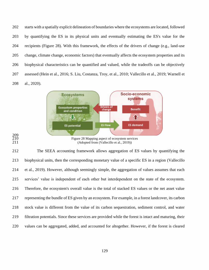
129
starts with a spatially explicit delineation of boundaries where the ecosystems are located, followed 202
by quantifying the ES in its physical units and eventually estimating the ES's value for the 203
recipients (Figure 28). With this framework, the effects of the drivers of change (e.g., land-use 204
change, climate change, economic factors) that eventually affects the ecosystem properties and its 205
biophysical characteristics can be quantified and valued, while the tradeoffs can be objectively 206
assessed (Hein et al., 2016; S. Liu, Costanza, Troy, et al., 2010; Vallecillo et al., 2019; Warnell et 207
al., 2020). 208
209 Figure 28 Mapping aspect of ecosystem services 210
(Adopted from (Vallecillo et al., 2019)) 211
The SEEA accounting framework allows aggregation of ES values by quantifying the 212
biophysical units, then the corresponding monetary value of a specific ES in a region (Vallecillo 213
et al., 2019). However, although seemingly simple, the aggregation of values assumes that each 214
services’ value is independent of each other but interdependent on the state of the ecosystem. 215
Therefore, the ecosystem's overall value is the total of stacked ES values or the net asset value 216
representing the bundle of ES given by an ecosystem. For example, in a forest landcover, its carbon 217
stock value is different from the value of its carbon sequestration, sediment control, and water 218
filtration potentials. Since these services are provided while the forest is intact and maturing, their 219
values can be aggregated, added, and accounted for altogether. However, if the forest is cleared 220

130
for timber harvesting, the values will be replaced by timber values or stumpage values. This system 221
of aggregation and stacking shows the potential tradeoff between identified ES. 222
The success of the experimental ecosystem accounting led to the UN Statistical 223
Commission's recent adoption as the framework to integrate the value of natural capital in 224
economic reporting (United Nations, 2021a, 2021b). The adoption of SEEA-Ecosystem 225
Accounting ensures that the accounting principles for including the value of natural capital as part 226
of the wealth and economic reporting adhere to the international standards. Simultaneously, the 227
methodologies and models used in the framework are widely accepted, particularly for valuing 228
ecosystem services and assets. This framework exposes the true wealth of a region and not only 229
considering its GDP. 230
While the ecosystem accounting framework advanced ES conservation approaches to 231
unprecedented progress, it is not without limits. Typically, the SEEA ecosystem accounting is done 232
on a large-scale area (e.g., regional, watershed, or national) (Vallecillo et al., 2019; Warnell et al., 233
2020). This is understandable since the framework's main objective is to account for the ES as part 234
of an economy. However, this approach becomes a challenge when looking at a specific parcel's 235
contribution to the overall landscape. The closest to looking at the contribution in a per parcel or 236
pixel level is using the ES models to estimate the biophysical account aspect of the SEEA 237
Ecosystem Accounting framework. 238
With the advancement in GIS and remote sensing technologies and ES quantification 239
models, ES models can highlight which specific ES are best produced in a particular pixel or region 240
(Fischer et al., 2019; Lawler et al., 2014; Lin et al., 2019; Paruelo et al., 2016; Schröter & Remme, 241
2016). Eventually, this can be used to identify, depending on a pixel’s resolution, which ES is 242
available in each pixel (Lin et al., 2019; Remme, Schröter, & Hein, 2014). However, one of the 243

131
limitations of this approach is that there is no comparable measurement of gains, losses, and 244
tradeoffs between different ES within a pixel brought by a particular land cover change since each 245
ES is treated separately within a pixel. Nevertheless, since land covers host multiple interconnected 246
ecosystems, any biophysical changes within the pixel affect the different ES simultaneously. 247
While accounting for the natural capital assets on a larger scale is critical for ES 248
conservation, knowing the per parcel contribution also has its important application, particularly 249
in the strategic implementation of conservation programs. Since conservation programs are 250
typically applied in portions of landowners’ parcels of land, a downscaled per pixel assessment 251
will help understand the effect of the intervention on ES production. Furthermore, a per-pixel 252
evaluation of the possible tradeoff of ES brought by land cover changes could provide effective 253
and strategic planning for landscape sustainability. Therefore, this study attempts to develop a 254
downscaled spatial accounting of ecosystem services using the tools approved in the SEEA 255
Ecosystem Accounting framework while also following its ecosystem accounting guidelines. 256
The primary objective is to create an ecosystem service-based index that can be applied 257
using pixel resolution as the basic spatial unit (BSU). This index is coined as the Spatial 258
Accounting of Ecosystem Services (SPACES) Index. Using the index, the study intends to account 259
for the net effect of each landcover type on the ecosystem service provision within the landscape. 260
Furthermore, using the SPACES Index counts the number of landcover pixels with high, positive, 261
neutral, and negative effects on the ecosystem service provision. 262
The study hypothesizes that a per pixel assessment of ecosystem service provision, such as 263
the SPACES Index, could provide detailed information for landscape sustainability planning. This 264
enhances sustainable land conservation strategies by identifying the hotspots for implementing 265

132
sustainable farming practices. Furthermore, this enables a way to assess the effectiveness of 266
sustainable practices being implemented in specific areas. 267
Methodology 268
The Ecosystem Accounting Framework 269
Developing the per pixel index starts from the System of Environmental-Economic 270
Accounting Ecosystem Accounting framework (Figure 29). The SEEA Ecosystem Accounting 271
begins with delineating the spatial coverage of ecosystems, followed by an accounting of the 272
condition of the ecosystems within the delineated coverage. It goes on to quantify the ES in the 273
delineated area and finally estimating the monetary value equivalent of the ES. However, for this 274
study to create the SPACES Index, we will utilize only the biophysical aspect of the ecosystem 275
accounting framework and not the estimation of the monetary value equivalent. 276
277 Figure 29 SEEA Ecosystem Service Accounting process flow 278
The ecosystem extent account uses basic spatial units (BSU) to subdivide the land areas 279
into a scaled and measurable coverage. This is represented through a geographic mesh, grid, or 280
pixel. Once the delineation of coverage is completed, information about the ecosystem per pixel is 281
obtained. Since these are remotely sensed using a geographically scaled resolution, pixel sizes can 282
be used as basic spatial units which contain ecosystem information. 283
The ecosystem condition account, also dependent on the spatial units, is used to define the 284
condition or state of the ecosystem in a specific BSU. For instance, suppose the BSU contains a 285
degraded ecosystem, i.e., a deforested area, the quality of the ES in that area is also affected; hence 286
Thematic account
Monetary asset
account
Ecosystem services account
Ecosystem condition account
Ecosystem extent
account
BIOPHYSICAL
SOCIO-ECONOMIC
133
it would reflect a low ES provision in the accounting sense. However, since ecosystem conditions 287
- particularly on a landscape level - are challenging to monitor, this information is simplified using 288
land cover as a proxy. This assumes that the identified land cover affects the ecosystem condition 289
and eventually the ES provision. 290
When the ecosystem extent and condition are established, a list of possible ES within a 291
spatial unit can be enumerated. Needless to say, that one BSU could contain multiple ES. 292
Determining the ES condition account is critical in the accounting framework. While this dictates 293
the state of the ecosystem and the services, it also identifies which ecosystem services should be 294
accounted for in a particular pixel. For example, in cases where the land cover is used as the 295
ecosystem condition, a forested area could provide multiple ES, including carbon stock, carbon 296
sequestration, and timber. Since timber production materializes when the tree is cut for utilization, 297
only then should it be considered in the accounting. Therefore, a standing forest land cover is most 298
likely attributed to carbon stocks and sequestration potentials rather than timber. However, if a 299
higher order of ecosystem condition is available, say land utilization information where it can 300
separately classify timberland from strictly protected land, then the ES attributed to the BSU could 301
change depending on if they are under timberland or protected land. Carbon stock could be 302
attributed to the BSU under the protected land, while timber production and its values could be 303
attributed to the timberland. 304
Furthermore, the ES condition also affects the possible interpretation of ES per pixel. For 305
instance, while water yield models estimate the overall water available in a delineated region, this 306
is done by aggregating the amount of water that flows to the stream as accumulated within the 307
area. However, suppose the model estimates the water yield potential per pixel as runoff, the 308
interpretation of the ES from the water yield per BSU as a surface runoff should be linked to its 309
134
implication, such as sediment export, nutrient runoff, and flood. For example, a BSU under a forest 310
land cover could have low water yield potential as compared to a BSU under an urban land cover 311
(J. C. Ureta, Clay, et al., 2020). This could be interpreted such that the BSU with a forest has lower 312
potential to release runoff as compared to the BSU with an urban land cover. Therefore, the ES 313
accounted for the specific BSU will be the ES associated with low surface runoff such as more 314
sediment and nutrient retention, higher infiltration rate, and prevention of flood. 315
With the advancement in remote sensing, Geographic Information System (GIS), and ES-316
based models, the amount of ES can be quantified per BSU. In the original SEEA framework, the 317
quantified ES is aggregated to make up the ES account, which is eventually used for estimating its 318
monetary value. While this approach is useful, the aggregation is done for the totality of the 319
delineated region and not within the BSU itself. This is because the ES have different physical 320
units; hence they cannot be summed up at the BSU level. Although, even without summing up the 321
ES within the BSU level, the quantified units per pixel provide critical information for landscape 322
sustainability planning. This has been the common approach for recording and understanding the 323
ES within the BSU (Remme et al., 2014; Sieber, Campagne, Villien, & Burkhard, 2021). 324
Therefore, for this study's purpose, while quantifying the ES uses similar models as adopted in the 325
SEEA framework (United Nations, 2014b, 2021a), we used the quantified ES units and created an 326
aggregation approach within each BSU by using an index. The index determines whether specific 327
BSU indicates an overall positive, negative, or neutral impact on the ES. 328
Spatial Accounting of Ecosystem Service Index 329
Indexes had been used in many different forms, while index creation has been developed 330
using different approaches. Indexes are used to assign measurable numeric values to a set of data 331
that indicates its relative importance, performance, or rank. Picking up from the ES quantification 332

135
process in the SEEA framework, since different ES will have different physical units, using an 333
index for each ES normalizes its values and makes them relatable to each other. 334
335 Figure 30 Process flow for developing the ES index 336
Figure 30 shows the process flow overview for converting the ES-based model outputs to 337
an ES index within a BSU. Eventually, since each ES index will be in the same scaled values, the 338
indexes can be summed up within the BSU to determine the net effect to the ES. The overall net 339
effect, termed as SPACES Index, becomes an indicator of how much ES is being produced within 340
a BSU by the current landcover. 341
To compute for the ES Index, we normalized the quantified physical units as estimated by 342
a separate ES-based model using the equation: 343
ESIij = ∑(𝑥𝑖𝑗−𝑥𝑚𝑖𝑛𝑗)
(𝑥𝑚𝑎𝑥𝑗 − 𝑥𝑚𝑖𝑛𝑗) (12) 344
Where ESIij is the index value of a particular ecosystem service j within a BSU i, and xij is the 345
quantified value in a physical unit of ES j within the BSU i. Furthermore, xmaxj is the overall 346
maximum quantified value of ES j in a physical unit, while xminj is the corresponding minimum 347
quantified value. The summation of ESIij constitutes the net effect of the landcover to the ES 348
provision and forms the SPACES Index. 349
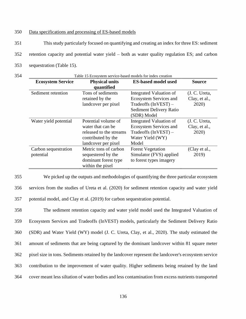
136
Data specifications and processing of ES-based models 350
This study particularly focused on quantifying and creating an index for three ES: sediment 351
retention capacity and potential water yield – both as water quality regulation ES; and carbon 352
sequestration (Table 15). 353
Table 15 Ecosystem service-based models for index creation 354
Ecosystem Service Physical units
quantified
ES-based model used Source
Sediment retention Tons of sediments
retained by the
landcover per pixel
Integrated Valuation of
Ecosystem Services and
Tradeoffs (InVEST) –
Sediment Delivery Ratio
(SDR) Model
(J. C. Ureta,
Clay, et al.,
2020)
Water yield potential Potential volume of
water that can be
released to the streams
contributed by the
landcover per pixel
Integrated Valuation of
Ecosystem Services and
Tradeoffs (InVEST) –
Water Yield (WY)
Model
(J. C. Ureta,
Clay, et al.,
2020)
Carbon sequestration
potential
Metric tons of carbon
sequestered by the
dominant forest type
within the pixel
Forest Vegetation
Simulator (FVS) applied
to forest types imagery
(Clay et al.,
2019)
We picked up the outputs and methodologies of quantifying the three particular ecosystem 355
services from the studies of Ureta et al. (2020) for sediment retention capacity and water yield 356
potential model, and Clay et al. (2019) for carbon sequestration potential. 357
The sediment retention capacity and water yield model used the Integrated Valuation of 358
Ecosystem Services and Tradeoffs (InVEST) models, particularly the Sediment Delivery Ratio 359
(SDR) and Water Yield (WY) model (J. C. Ureta, Clay, et al., 2020). The study estimated the 360
amount of sediments that are being captured by the dominant landcover within 81 square meter 361
pixel size in tons. Sediments retained by the landcover represent the landcover's ecosystem service 362
contribution to the improvement of water quality. Higher sediments being retained by the land 363
cover meant less siltation of water bodies and less contamination from excess nutrients transported 364

137
by the sediments to the stream, leading to a better quality of water in streams and rivers (J. C. 365
Ureta, Clay, et al., 2020). 366
On the other hand, the estimated potential water yield represents the volume of water that 367
the landcover releases as it flows to the water bodies. Due to this, while the aggregated volume for 368
the whole region could be interpreted as a contribution to water supply, the per-pixel interpretation 369
must be construed as surface runoff. Hence, higher surface runoff correlates to higher sediment 370
export, a higher likelihood of flooding, and declining water quality (J. C. Ureta, Clay, et al., 2020). 371
Finally, the carbon sequestration potential was estimated by using the carbon stocks data 372
acquired by the Forest Inventory Analysis (FIA) to the Forest Vegetation Simulator (FVS). Once 373
the carbon sequestration potential per forest type was computed, it was applied to the remotely 374
sensed forest type map to calculate the carbon sequestration potential per land cover (Clay et al., 375
2019). While the FVS provided a comprehensive estimate of the carbon sequestration potential for 376
the forest land cover, it does not cover other vegetations such as agriculture, grassland, and 377
pastureland due to data availability. Therefore, the carbon sequestration potential was only applied 378
to the forest land cover. 379
At this point, it is important to define the interpretation of the ecosystem service being 380
accounted for per pixel as it determines whether the land cover affects the ecosystem service either 381
positively or negatively. Therefore, particularly for this study, the amount of sediments being 382
retained and carbon sequestered is positively affected by the land cover. At the same time, the 383
water yield potential, since it is interpreted as runoff, is considered to be negatively affected. 384
Furthermore, it is also important that the pixel sizes are similar across the models’ outputs to 385
maintain the correct information per pixel. Therefore, all raster outputs were resampled to have a 386
9m x 9m resolution, making each pixel cover an area of 81 square meters on the ground. The 387

138
creation of the indexes and aggregation of each index is done using the ArcGIS raster calculator 388
function through ArcGIS Pro 2.7.2 version. 389
Index Limitation 390
The development of the SPACES Index allows for a measurable indicator of ecosystem 391
services condition on a pixel level. This opens up new opportunities for landscape sustainability 392
planning, monitoring, and ES-based conservation programs. However, just like any other indexes 393
and model, using the SPACES index score is not without limitations. 394
First, the ES-based model’s efficacy and accuracy significantly affect the SPACES index. 395
Since the SPACES index collects and streamlines the ES-based model outputs, it essentially 396
becomes the SPACES index inputs. Therefore, it is important that the quality of the ES-based 397
model’s output be accurate for the SPACES index to be effective and reliable. Due to this, the 398
boundaries and pixel resolution of all ES-based model output that flows to the index must be the 399
same. 400
Second, the SPACES Index scores apply specifically to the pixels within the delineated 401
contiguous region. Hence, the scores reflect the performance of the ES condition of a pixel in 402
relation to other pixels within the region. The index scores cannot be used in areas outside of the 403
delineated region. However, if sub-regions exist, then the index scores within and between 404
subregions can be used. Therefore, the initial delineation of the overall landscape is important for 405
the index. 406
Finally, the landcover data significantly affects the SPACES index, ES indexes, and ES-407
based models since the pixel resolution and ecosystem condition are based on landcover resolution; 408
hence, it is important that the landcover data input is the latest and most detailed. However, most 409

139
landcover datasets are based on coarse satellite imagery (30m x 30m per pixel) and a compiled 410
classification system, particularly for forest and agriculture landcover. 411
The coarse resolution aggregates the dominant landcover within a pixel; therefore, small 412
green spaces such as easement areas are less likely to reflect the ecosystem condition within the 413
pixel accurately. While the resampling technique can convert the pixel sizes to a finer resolution 414
(i.e., 9m x 9m per pixel), the information that each pixel will retain still comes from the coarse 415
input source. This can be improved if a land utilization or land-use imagery is available. A land-416
use imagery captures an image of the land with more significant details. This could be done by 417
using higher resolution satellite imagery or through ortho photogrammetry. However, higher 418
resolution data inputs require more processing power, longer processing time, and more extensive 419
storage for data and image archiving. 420
In addition, while the generalized classification of land covers is advantageous for 421
retroactive comparison of land covers, it poses a limitation when determining the ecosystem 422
condition per index. The ecosystem condition defines the list of possible ES in each pixel, and 423
different species within the ecosystem affect other coefficients that lead to the amount of ES it 424
produces. For instance, the amount of sediment retained by an apple orchard is different from a 425
corn field because the crop management and support practice factors differ. To mitigate this, the 426
landcover data input must be reclassified to reflect the most detailed information available by 427
combining different landcover-based data inputs such as the Crop Data Layer (CDL) for including 428
different crops within the agriculture landcover (USDA-NASS, 2019b). 429
Study site 430
The study is conducted at the Santee River Basin Network (SRBN) in South Carolina 431
(Figure 31). The river basin originates from the highland ridges of southern North Carolina (NC) 432

140
and traverses SC up to its coast. The administrative jurisdiction is subdivided into three regions: 433
Upstate, Midland, and Lowcountry and Coastal (SC Area Health Education Consortium (AHEC), 434
n.d.). While AHEC regional subdivision is used for health education, this represents the socio-435
economic aggregation based on administrative jurisdiction per region. The landscape is home to 436
approximately 79% of the population (United States Census Bureau, 2018), with major cities of 437
Greenville at the Upstate; Columbia at the Midland; and Charleston at the Lowcountry and Coastal 438
regions. Overall, the SRBN covers approximately 7.54 million acres wherein 2.1 million acres 439
cover the Upstate, 3.8 million acres cover the Midland, and 1.6 million acres cover the Lowcountry 440
and Coastal region (USDA-NASS, 2019b). 441
442 Figure 31 The Santee River Basin Network as study site divided by region (Upstate, Midland, Lowcountry and 443
Coastal) 444

141
The landcover distribution of SRBN and its regions is summarized in Table 16. The highest 445
landcover concentration in the Upstate and Midland region is forest land, while for the Lowcountry 446
and Coastal region is woody wetland. Furthermore, the highest concentration of agricultural land 447
cover is in the Lowcountry and Coastal region. In terms of urban and developed land, the highest 448
concentration is at the Upstate, followed by the Midland, and Lowcountry and Coastal. 449
Table 16 Land cover distribution per region (in %) 450
Land cover Upstate Midland Lowcountry and Coastal Overall SRBN
Agriculture 3.07 3.16 6.05 3.76
Barren 0.45 0.48 0.37 0.45
Developed/Urban 18.41 11.50 9.47 13.00
Forest 56.29 60.34 22.93 51.13
Grassland/Pasture 17.35 10.77 1.82 10.69
Herbaceous Wetland 0.02 0.17 5.26 1.23
Idle Cropland 0.06 0.25 0.23 0.19
Shrubland 1.99 3.38 9.52 4.31
Water 1.58 2.93 10.44 4.17
Woody Wetland 0.78 7.02 33.91 11.07
Results and Discussion 451
Generating the SPACES Index 452
Following the methodologies on quantifying the three ecosystem services (Clay et al., 453
2019; J. C. Ureta, Clay, et al., 2020) - sediment retention, water yield potential, and carbon 454
sequestration; we were able to transform the physical units into their ES indexes counterpart 455
through the statistical normalization technique. The results of the normalized ES indexes are 456
shown in Figures 32a, 32b, and 32c. Since the ecosystem services sediment retention and carbon 457
sequestration have been interpreted in terms of benefits, the scale of their ES indexes took a value 458
of 0 to 1. On the other hand, for the water yield potential per pixel, since the values were interpreted 459
in terms of a negative impact through surface runoff, the scale of their ES indexes took a value of 460
0 to -1. The summation of all the indexes per pixel constitutes their Spatial Accounting of 461

142
Ecosystem Services Index (Figure 32d). Since each ecosystem services’ physical unit was 462
normalized and rescaled into a similar range, the ES indexes can be added all together to estimate 463
the net impact. However, with the lack of weighting considerations per ecosystem service, this 464
approach assumes that each ES is equally important and has the same effect on human well-being. 465

143
(a) Sediment Retention ES Index
(d) SRBN Spatial Accounting of Ecosystem Services Index
(b) Carbon Sequestration ES Index
(c) Water Yield Potential ES Index
Figure 32 ES Index to SPACES Index
144
The generated SPACES index is expected to yield a value ranging from -1 to 2. The best-466
case scenario of a pixel will yield 2 if and only if the sediment retention index is 1, the carbon 467
sequestration index is 1, while the water yield potential is 0. On the other hand, the worst-case 468
scenario of a pixel will yield a -1 if and only if the sediment retention index is 0, the carbon 469
sequestration index is 0, while the water yield potential is -1. Overall, the SPACES Index values 470
in SRBN yielded a mean value of 0.02, with a standard deviation of 0.2, a minimum value of 0.9, 471
and a maximum value of 1.4. 472
Considering this range, we reclassified the ES index to: “less than -0.7”, “-0.7 to -0.2”, “-473
0.2 to 0.2”, “0.2 to 0.7”, “greater than 0.7”. Since no existing standard ES index is currently being 474
used, the reclassification was arbitrary and primarily based on the standard deviation and mean. 475
Pixels within the standard deviation and mean were classified “Neutral”; hence the landcover’s 476
effect does not positively nor negatively affect the ES provision. While pixels with negative values 477
beyond the standard deviation were classified as “Negative,” meaning the landcover affects the ES 478
negatively. Moreover, pixels with positive values beyond the standard deviation represent areas 479
where the landcover affects the ES positively. Finally, while the delineation was arbitrary, pixels 480
with ES index value greater than 0.7 were classified as High ES areas. The High ES areas were 481
singled out to emphasize the locations of pixels that yield the most ES, hence possibly indicating 482
high sediment retention capacity, high carbon sequestration, and low water yield potential. 483
Using ArcGIS Pro 2.7.2, the information of a selected specific pixel can be revealed. This 484
contains the ES index value of each ecosystem service and the SPACES index value of the pixel. 485
Figures 6a, 6b, 6d, and 6e show sample pixels' contents with high, positive, neutral, and negative 486
SPACES Index classification. 487
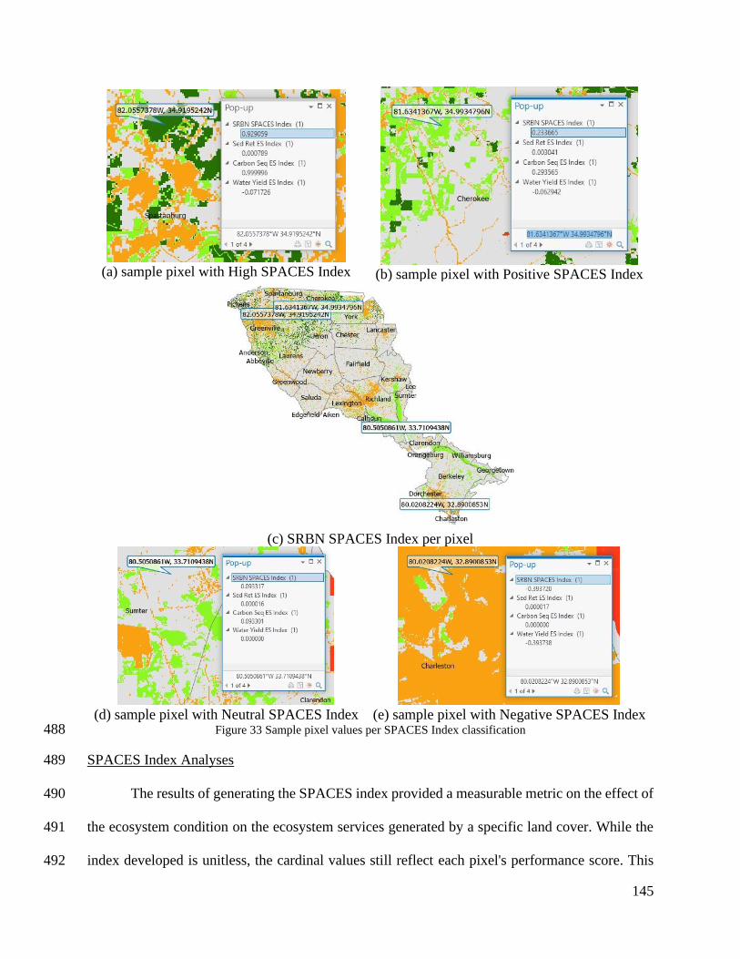
145
(a) sample pixel with High SPACES Index
(b) sample pixel with Positive SPACES Index
(c) SRBN SPACES Index per pixel
(d) sample pixel with Neutral SPACES Index
(e) sample pixel with Negative SPACES Index
Figure 33 Sample pixel values per SPACES Index classification 488
SPACES Index Analyses 489
The results of generating the SPACES index provided a measurable metric on the effect of 490
the ecosystem condition on the ecosystem services generated by a specific land cover. While the 491
index developed is unitless, the cardinal values still reflect each pixel's performance score. This 492

146
allows us to perform mathematical operations such as aggregation of SPACES index scores by 493
land cover type or within a specific area or polygon and further inferential statistical analysis. 494
Furthermore, the reclassification of the SPACES Index scores emphasized the location of sites 495
where land covers have “high,” “positive,” or “negative” effects on the ecosystem service. 496
Regional analysis 497
The SPACES Index map of SRBN was subdivided into each region (see Appendix N, O, 498
and P). The best-case scenario for an ecologically sustainable landscape is for most pixels to have 499
positive index scores, which are indicated as green pixels in the map. However, the resulting map 500
of all regions shows that majority of the pixels are gray. This means that the index score of the 501
pixels is within the acceptable standard deviation (0.2) from the mean (0.02). This can be treated 502
as land covers that have a neutral effect on the ecosystem services. While gray pixels indicate 503
neutrality, this also presents an opportunity to identify potential areas that could have a high 504
likelihood to be rehabilitated and turn to green pixels, especially if the gray pixels are adjacent or 505
within the cluster of green pixels. In contrast, it can also identify potential areas that could be 506
immediately threatened to turn orange, which are negative pixels, particularly if the gray pixels 507
are adjacent or within the cluster of the orange pixels. 508
Results of the Upstate region map, particularly the areas from the southern part of the 509
counties Greenville and Anderson, the central to the southern area of Spartanburg county, the 510
central to the northern area of Lauren county, and the county of Abbeville suggest opportunities 511
to improve the pixels from gray to green. On the other hand, the expanding urban area in the county 512
of Greenwood seems to be more likely to turn orange. Finally, the area on the north of Greenville 513
county and the whole of Pickens county shows to have pixels with high index scores; however, 514
these could be threatened by the expanding urban area from the center. 515
147
In the Midland region, areas with a high likelihood for improving the index scores can be 516
found at the eastern part of Cherokee county, the central area of York, the northern part of 517
Lancaster, and the river and wetland areas at the southern boundary of Kershaw, southeast of 518
Richland, and northeast of Sumter. Furthermore, pixels with high index scores can be found at the 519
central to the northern part of Union, and along the boundaries of Cherokee and York. On the other 520
hand, areas with a high concentration of pixels with negative index scores are in Lexington county, 521
the central area of Richland county, some areas at the central part of Kershaw and Lancaster, and 522
a possibly growing area at the central part of Newberry. 523
Finally, for the Lowcountry and Coastal region, the map suggests that areas at the central 524
part of Berkeley county, some part at the north of Calhoun county, and along the wetland and river 525
side of the counties Clarendon, Williamsburg, and Georgetown could have a high likelihood for 526
ES improvement. On the other hand, pixels with negative index scores are concentrated on the 527
southwestern part of Berkeley county, the southeastern part of Dorchester county, and Charleston 528
county. 529
Overall, the results show that areas with high and positive index scores coincide with 530
vegetated areas, while pixels with negative index scores overlap with non-vegetated areas. This 531
was validated by analyzing the cardinal values of the index scores per pixel by its land cover type 532
across the three regions (Table 17). The SPACES index aggregated to obtain the overall index 533
score that can be computed for each of the landcover across the three regions. Furthermore, the 534
index classification was tallied to show the frequency distribution of each class for each landcover 535
which could indicate a possible trend that connects to the total index score. 536
Table 17 Summary statistics of SRBN's SPACES Index by landcover and by region 537
Reg Landcover Area
(acres) SPACES Index
Relative frequency of pixel
classification

148
SPACES
Index
Total Score
Mean
SPACES
Index per
acre
%
Pixels
High
%
Pixels
Pos
%
Pixels
Neut
%
Pixels
Neg
Up
stat
e
Agriculture 51,882 -74,059 -1.43 0.04% 1.16% 97.36% 1.44%
Barren 7,689 -136,090 -17.70 0.00% 0.46% 0.02% 99.53%
Developed/Urban 313,638 -7,494,594 -23.90 0.00% 0.12% 0.01% 99.88%
Forest 954,326 8,334,760 8.73 0.69% 7.02% 90.92% 1.38%
Grassland/Pasture 293,975 -358,995 -1.22 0.14% 2.53% 94.52% 2.81%
Herbaceous
Wetland 260 1,236 4.75 0.03% 10.59% 89.39% 0.00%
Idle Cropland 1,066 -23,555 -22.11 0.00% 0.31% 0.01% 99.68%
Shrubland 33,849 231,492 6.84 0.69% 6.98% 89.85% 2.48%
Water 27,067 -212,846 -7.86 0.00% 0.30% 6.85% 92.84%
Woody Wetland 13,283 173,538 13.06 0.60% 35.20% 64.20% 0.00%
Mid
land
Agriculture 95,028 -242,257 -2.55 0.18% 0.84% 96.84% 2.14%
Barren 14,710 -424,565 -28.86 0.00% 1.99% 0.54% 97.48%
Developed/Urban 345,680 -10,853,921 -31.40 0.00% 0.73% 0.47% 98.80%
Forest 1,822,676 6,967,169 3.82 4.18% 7.43% 87.41% 0.98%
Grassland/Pasture 322,980 -785,051 -2.43 1.06% 2.10% 96.17% 0.66%
Herbaceous
Wetland 5,190 35,341 6.81 0.46% 31.09% 68.45% 0.00%
Idle Cropland 7,455 -246,185 -33.02 0.00% 0.14% 0.25% 99.61%
Shrubland 102,439 108,681 1.06 1.90% 6.20% 90.72% 1.18%
Water 88,158 -613,992 -6.96 0.19% 0.20% 97.06% 2.55%
Woody Wetland 214,905 2,114,440 9.84 0.84% 45.94% 53.22% 0.00%
Lo
wco
untr
y &
Coas
tal
Agriculture 78,059 -166,951 -2.14 0.04% 0.20% 98.33% 1.44%
Barren 4,370 -118,524 -27.12 0.00% 0.46% 0.09% 99.46%
Developed/Urban 118,370 -3,714,948 -31.38 0.00% 0.12% 0.10% 99.79%
Forest 296,252 343,581 1.16 0.69% 0.94% 97.01% 1.35%
Grassland/Pasture 23,640 -83,366 -3.53 0.14% 0.30% 96.76% 2.81%
Herbaceous
Wetland 56,840 209,775 3.69 0.03% 10.17% 89.80% 0.00%
Idle Cropland 3,040 -88,675 -29.17 0.00% 0.31% 0.86% 98.83%
Shrubland 122,667 -59,655 -0.49 0.69% 1.04% 95.80% 2.47%
Water 105,036 -1,013,663 -9.65 0.01% 0.01% 96.06% 3.92%
Woody Wetland 442,137 3,616,879 8.18 0.60% 32.28% 67.13% 0.00%
Consistent across the regions, the land covers with positive Total SPACES index are the 538
vegetated areas particularly, forest, shrubland, and wetland. The frequency of high and positive 539
index scored pixels also supports the total index score. Particularly for the Upstate region, the 540

149
positive and high areas are at the forest and shrubland, forest and wetland area for the Midland 541
region, and wetland areas for the Lowcountry and Coastal region. 542
While the forest land cover provides significant sediment retention capacity, the vastness 543
of the area coverage releases voluminous water, particularly for those in the Upstate region since 544
these forests are typically located primarily at the head waters where slopes are steep (J. C. Ureta, 545
Clay, et al., 2020), therefore affecting their SPACES index. However, with the inclusion of carbon 546
sequestration, since the model quantified the carbon sequestered primarily by the forest ecosystem 547
that is eligible in the carbon market framework (Clay et al., 2019), hence other land covers are 548
treated to have very low or minimal carbon sequestration potential. Nevertheless, even in different 549
regions and discounting the effect of carbon sequestration, forest land covers still provide high or 550
positive index since they have high sediment retention capacity and low potential water yield 551
runoff per pixel compared to other land covers (J. C. Ureta, Clay, et al., 2020). 552
On the other hand, despite the minimal carbon sequestration included in the model, other 553
areas with positive SPACES index coincide with wetlands and shrubland areas. This could be 554
associated with the potential water yield ES since these land covers are primarily vegetated (J. C. 555
Ureta, Clay, et al., 2020). Vegetated land covers consume water and holds captured water in place 556
for a more extended period of time as compared to non-vegetated areas. This contributes to the 557
infiltration rate and eventually to ground water recharge, as well as improvement to soil quality 558
since nutrients, sediments, and soil organic matter are not eroded by the potential runoff (Clay et 559
al., 2020; J. C. Ureta, Clay, et al., 2020) 560
On the other hand, the concentration of areas with negative index scores coincide with 561
highly urbanized areas, particularly in the counties of Greenville and Spartanburg at the Upstate 562
region, York, Lexington, and Richland at the Midland region, and Dorchester, Berkeley, and 563
150
Charleston at the Lowcountry and Coastal region. Similarly, developed areas such as roads and 564
other non-vegetated areas such as barren and idle cropland emphasized its negative index scores 565
in the maps. 566
Finally, while grassland and agricultural land are also considered vegetated areas, the 567
overall index score indicates a negative value. This could be because the sediment retention 568
capacity for these areas is low. And while the potential water yield is also low compared to non-569
vegetated areas, it could be slightly higher than the sediment retention index. This can be observed 570
by comparing the mean SPACES index per acre of these land covers, which are substantially lower 571
than non-vegetated land covers. Furthermore, since the carbon model does not include the carbon 572
sequestration potential from these vegetated land covers, this could also be why their index turned 573
out to be negative. 574
Specific area analysis 575
Following the aggregation method per landcover using the cardinal values of the SPACES 576
index, this was also used to estimate the index score of a specific area or polygon in a given 577
location, such as easements, protected areas, or designated parks. Using the extracted polygons of 578
conservation areas within SRBN using the Protected Area Database (US Geological Survey 579
(USGS) Gap Analysis Project (GAP), 2012), we computed for the SPACES index of each 580
conservation area such as for the Congaree National Park (Figure 34) 581
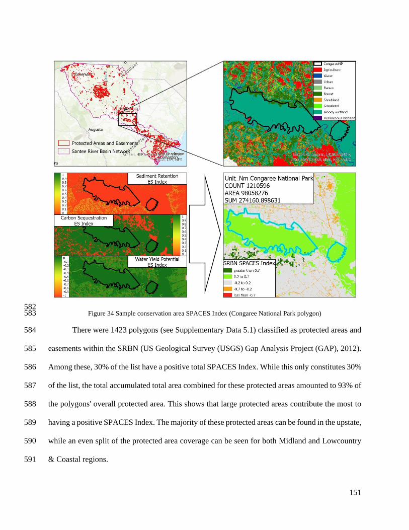
151
582 Figure 34 Sample conservation area SPACES Index (Congaree National Park polygon) 583
There were 1423 polygons (see Supplementary Data 5.1) classified as protected areas and 584
easements within the SRBN (US Geological Survey (USGS) Gap Analysis Project (GAP), 2012). 585
Among these, 30% of the list have a positive total SPACES Index. While this only constitutes 30% 586
of the list, the total accumulated total area combined for these protected areas amounted to 93% of 587
the polygons' overall protected area. This shows that large protected areas contribute the most to 588
having a positive SPACES Index. The majority of these protected areas can be found in the upstate, 589
while an even split of the protected area coverage can be seen for both Midland and Lowcountry 590
& Coastal regions. 591

152
Since the SPACES index scores transform the landcover pixels to have a continuous value 592
that measures their ecosystem services, the values can be analyzed inferentially to understand other 593
factors that could affect the index scores. For instance, we employed linear regression analysis to 594
understand the contribution of the protected area characteristics to the index scores (Table 18). 595
Table 18 Linear regression of Protected Area SPACES Index scores 596
Characteristic Coefficient P-value
Area 0.001 0.000
Upstate 746.346 0.271
Midland 1124.338 0.057
Restricted Access 2226.984 0.037
Closed Access -1622.760 0.058
_cons -497.269 0.316
N = 1423
R-squared = 0.9424
Adj R-squared = 0.9422
Results suggest that in terms of area, the greater area coverage of conservation polygon 597
associates with an improved index score. While in terms of regional characteristics, conservation 598
areas in the Midland seem to be better off than the Lowcountry and Coastal, while Upstate 599
conservation areas have no statistically significant difference from the Lowcountry and Coastal 600
areas. Finally, results also show that Restricted access improves the SPACES index of protected 601
areas compared to Open access. In contrast, Closed Access shows to have lower SPACES index 602
as compared to Open access. This suggests that a certain level of access to the conservation areas 603
could improve its ecosystem services provision performance. 604
Conclusion 605
This study presents a novel approach in landscape sustainability planning and monitoring 606
by developing an ecosystem-serviced based performance index called Spatial Accounting of 607
Ecosystem Services (SPACES) index. With the adoption of the System of Environmental-608
Economic Accounting by the United Nations, the ecosystem accounting framework and its 609
153
methodologies established a novel approach. Therefore, this study picks up the framework to be 610
applied to a more granular level, allowing measuring the ES provision performance of different 611
landcover pixels across the landscape. 612
The SPACES index aggregates and mainstreams the outputs of various spatial ES-based 613
models through a normalization process. The normalized values of each ES-based model are 614
stacked and aggregated within its basic spatial unit hence associating the index scores with its 615
spatial attributes. The index score reflects how the ecosystem condition affects the quantities of 616
ecosystem service produced within a pixel. In this study, since the landcover dataset represents the 617
ecosystem condition, the index scores essentially measure the ecosystem service provision 618
capacity of the landcover within the pixel. 619
With the SPACES index scores present in each pixel, this provides a measurable metric 620
that indicates a specific pixel's ecosystem service provision capacity. Hence, further statistical and 621
geographic analysis can be made. For instance, particularly for the Santee River Basin Network 622
(SRBN) of South Carolina, the index highlighted that forests, wetlands, and shrubland areas 623
provide the most ES compared to other land cover types. Furthermore, it also showed the exact 624
location of pixels where possible improvements for strategic conservation planning can be 625
implemented in each region. On the other hand, the index also highlighted the effect of non-626
vegetated areas on ES provision, particularly the growing urban land cover. This emphasizes that 627
while urbanization provides economic development, a tradeoff between the ES provision also has 628
to be considered. 629
Finally, utilizing the SPACES index creates an approach to assign a collective scoring 630
mechanism to a specific subject area, such as conservation easements and protected areas. The 631
collective score approximates the ES provision status of the easements. While the information is 632
154
simply an indication, it still offers essential insights in managing conservation areas. Furthermore, 633
the collective scores can assess other factors that can improve conservation area management. In 634
the case of SRBN, large delineated conservation areas suggest doing best in ES provision. 635
Further improvements are also important to make the index more comprehensive. First, the 636
index could be expanded by including other spatially attributable ecosystem services (i.e., 637
pollination ES, wildlife habitat, air quality improvement, etc.) Including more ES-based models 638
paint a better and bigger picture of ES provision per pixel. Secondly, since the SPACES index 639
only includes physical quantities of ES, it does not account for the socio-economic factors that 640
coincide in each pixel. Integrating the socio-economic aspect in the index could improve the 641
assessment of tradeoffs associated with each pixel. Lastly, using high-resolution land-use maps 642
enhances the representation of ecosystem conditions. With the advancement in remote sensing and 643
unmanned aerial vehicle or drone technologies, coupled with powerful processing software to 644
handle big data, the processing approach of ES-based models and the index creation could improve 645
drastically. This will provide better and more comprehensive information for sustainable landscape 646
management. 647
Despite its limitations, the use of the SPACES index provides an advancement towards a 648
quantifiable approach to monitoring the quality of the ecosystem condition, the ability of the 649
ecosystem to provide its services, and the state of the flow of ecosystem services that affect human 650
well-being. Hence, it offers many opportunities and possibilities in applying ES-based strategic 651
measures to a specific location. In this manner, managers are more equipped and connected to 652
ecosystem services in implementing sustainable practices across the landscape. 653
155
CHAPTER SIX 654
655
PES: A WAY FORWARD 656
657
It is without question that development and economic growth are essential for societal 658
progress. However, the increasing rate of economic progress compromised the quality of the 659
environment and affected the ecosystems and their services. This becomes a “chicken-and-egg” 660
phenomenon where society asks which, between economic growth and environmental 661
conservation, must be prioritized. While human nature focuses on the betterment of our well-being, 662
we tend not to notice the impact on the source of this development. This is partly because economic 663
development results are more tangible, directly connected to our lifestyle, and can easily manifest 664
in our society. On the other hand, the consequences of our rapidly increasing economic 665
development to the environment are less noticeable, most often are indirectly connected to our 666
daily lifestyle, and builds gradually until it becomes a phenomenon that can bring significant 667
damages (i.e., biodiversity loss, aggravating climate change impacts, etc.) However, with the 668
advent of clean technologies, conservation sciences, and sustainable development, new 669
opportunities for creating a synergistic relationship between economic growth and environmental 670
conservation ensues under the sustainability framework. 671
In many areas, due to the rate of urban expansion, land conversion has been steadily 672
increasing since land values are seen to be more lucrative to be used for economic and industrial 673
purposes. This continues because the land values accounted for only include monetary value and 674
not accounting for non-monetary value, which is essential for the overall well-being. One approach 675
to mitigate this is by implementing conservation programs. Particularly, landowners are 676
encouraged to allocate land areas devoted to conservation activities rather than utilize it for 677
conventional production or convert it to urban and industrialized spaces. In exchange, landowners 678

156
are compensated for keeping their land and implementing conservation activities. However, 679
conservation programs incur costs that may not be sustainable in the long run. Therefore, the 680
Payments for Ecosystem Services (PES) scheme, a type of sustainable financing mechanism, can 681
be created to support the implementation of these programs. The PES creates a stakeholder-driven 682
platform where funds can be sought for and continuously sustain the conservation program 683
implementation. The primary focus of the scheme is to ensure the provision of ecosystem services 684
(ES) by creating a symbiotic relationship between ES providers (ES sellers) and ES recipients (ES 685
buyers). The PES framework creates a market-like system where ES sellers ensure a healthy 686
environment and ecosystem, which is a source of the ES being provided to its recipients – the ES 687
buyers. In exchange, the ES buyers provide financial or in-kind provision, which is used to 688
compensate and support the ES sellers. While PES seems straightforward, designing the 689
framework has to be systematic to ensure its feasibility. Therefore, this study created a systematic 690
approach to develop a PES in the Santee River Basin Network (SRBN) of South Carolina. The 691
systematic process of this study features a PES design that: a) stakeholder-driven; b) with 692
scientifically sound evidence and linkages of ecosystem services to its recipients; c) with 693
systematic analysis of stakeholders’ preference and capacity to support the program; and d) can 694
provide a precise strategic location where conservation programs can be implemented. 695
Integrating the results of the chapters from this study completes the elements in 696
systematically designing a PES in SRBN. By understanding the stakeholders' preferences, we have 697
identified that the priority ES that stakeholders will support are water-related ES, particularly water 698
quality improvement. Due to this, we quantified the amount of ES provided by the landcover per 699
pixel using the Integrated Valuation of Ecosystem Services and Tradeoffs (InVEST) models. The 700
Sediment Delivery Ratio (SDR) model for estimating the sediment retention capacity and the 701
157
Water Yield (WY) model estimate the amount of water potentially captured by a pixel of a 702
landcover. We used these quantities to evaluate the possible change of potential sustainable 703
practices that can be implemented, classified as crop-based practice using cover crops or tree-704
based practice with agroforestry farming. The possible change was presented to stakeholders to 705
elicit their willingness to pay to support the program. This establishes that stakeholders are willing 706
to support the program and that the PES scheme can gain traction and be feasibly implemented in 707
SRBN. Finally, the development of the SPACES index by combining the outputs of different ES-708
based models emphasized the specific locations and conditions where ES can be improved or 709
rehabilitated. With this, landscape managers can decide where conservation programs can 710
strategically be implemented and how much coverage the PES scheme supports. 711
A key result of the study is that vegetated land covers provide the most ES, particularly the 712
forest land area. However, while another key result is that stakeholders are willing to pay to 713
improve the ES of vegetated areas, the SRBN is too vast and only patches of forest landcover can 714
be prioritized. Therefore, picking these results up and utilizing the SPACES index output to locate 715
the specific areas for ES improvement creates an opportunity to form a PES mechanism in a sub-716
regional, localized, or even smaller scale. In this manner, the potential PES drivers will be locally 717
instituted, and the PES elements will have a direct connection to each other. Essentially, making 718
the local PES scheme a community-based sustainable financing mechanism. This opens up more 719
opportunities for community-based conservation efforts and ease of introducing new approaches 720
such as agroforestry farming. 721
Another key result in the study is the benefits of utilizing cover crops as a sustainable 722
farming practice. However, there is a low adoption rate of the practice from the farmers. Since 723
stakeholders are willing to pay for crop-based farming techniques, a PES scheme targeting major 724
158
agricultural areas can be formed to jump-start the support for this program. Furthermore, this can 725
be improved by identifying strategic agricultural areas adjacent to landcovers rich in ES provision 726
to maximize its effect. 727
While designing a feasible PES scheme offers promising possibilities in conservation and 728
resource management, the actual implementation poses different challenges. Operationalizing the 729
PES requires further stringent steps. This includes: 1) careful negotiation of a binding agreement 730
between PES parties; 2) assessing the capacity of ES sellers to provide the ES continuously and 731
their willingness to accept (WTA) to engage in the PES scheme; 3) establishment of fund 732
collection, disbursement, audit, and reporting system; 4) development of marketing strategies for 733
public awareness and support; 5) developing a monitoring and evaluation system; and lastly, 6) 734
involving the relevant institutions to drive and ensure that the PES scheme is meeting its objectives 735
- all of which have not been covered in this study. Nevertheless, this study, albeit preliminary for 736
a PES scheme, already presents critical information applicable to manage the Santee River Basin 737
Network sustainably. 738
Overall, this study presents that sustainable financing mechanism such as the PES scheme 739
enhances the way we implement conservation programs. Furthermore, stakeholders’ involvement 740
in conservation opens up new possibilities in managing the landscape. Ultimately, while there is 741
increasing demand and rapidly rising economic progress, it does not have to compromise the 742
quality of the environment. With the existing and further development of new technologies and 743
sustainable approaches, balancing economic growth and environmental conservation is becoming 744
more probable, leading to sustainable development. 745
746

159
747
748
749
750
751
752
753
754
755
756
757
758
759
760
761
762
763
764
765
766
767
768
769
770
APPENDICES 771 772
160
Appendix A 773
Survey questionnaire for knowledge, awareness, and perception survey 774
Land Owners and Residents’ Perception of Conservation in South Carolina 775 776
Section I: Introduction 777 778
You have been randomly selected to participate in a survey being conducted by researchers at Clemson 779 University, Baruch Institute of Coastal Ecology and Forest Science. 780 781 You will be asked to respond to questions on your perception, views, and satisfaction towards 782 environmental and resource conservation, activities, and potential or actual impacts brought about by 783 these types of intervention. You are free to NOT ANSWER any of the questions. 784 785 Conservation is the act of preserving, protecting, or restoring the environment, ecosystems, vegetation, 786 and wildlife. Policies and best management practices are implemented to sustain the state’s significant 787 natural resource lands, wetlands, historical properties, archeological sites, and urban parks. Resource 788 conservation in SC provides jobs in areas of agribusiness, forestry, tourism, and other sectors. As a matter 789 of fact, tourism supports one-tenth of the state’s jobs and generates about $ 1.9 billion annually in the 790 state’s economy. To further improve the implementation and management of these practices for its 791 citizens' well-being, this survey intends to evaluate perceptions, satisfaction, and understanding of 792 stakeholders towards environmental conservation and natural resource management in South Carolina. A 793 deeper understanding of the citizens’ view point would definitely lead to better policies, conservation 794 efforts, and best management practices of South Carolina’s abundant natural resources. 795 796 Your participation in the interview will be VOLUNTARY. Your refusal to participate in or to withdraw 797 from the study carries no penalty or loss of any benefits. The information that you provide will be kept 798 CONFIDENTIAL and will not be released to any other entity that is not involved in the study. No one 799 will know your answers but our research team, and your identity will be protected in any report based on 800 the data. 801 802 Your participation in the survey is critical and the results could be used to further improve the 803 conservation efforts for our natural resources while also helping to improve the welfare of residents of 804 SC. We hope you can help us by participating in this survey. If you do agree to participate in this survey, 805 please answer the questions as best you can. 806 807 If you are willing to participate, please proceed to the succeeding questions. 808 809 I.1 What county do you live in? 810 I.2 What is your zip code? 811 812
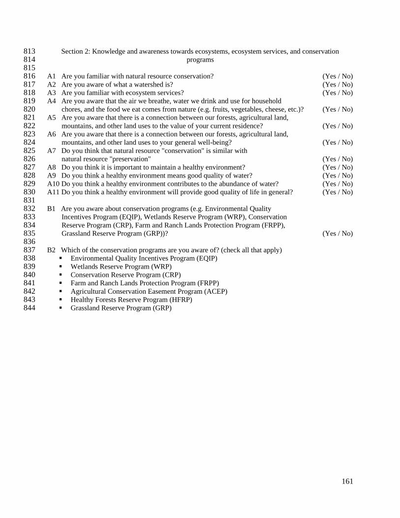
161
Section 2: Knowledge and awareness towards ecosystems, ecosystem services, and conservation 813 programs 814
815 A1 Are you familiar with natural resource conservation? (Yes / No) 816 A2 Are you aware of what a watershed is? (Yes / No) 817 A3 Are you familiar with ecosystem services? (Yes / No) 818 A4 Are you aware that the air we breathe, water we drink and use for household 819 chores, and the food we eat comes from nature (e.g. fruits, vegetables, cheese, etc.)? (Yes / No) 820 A5 Are you aware that there is a connection between our forests, agricultural land, 821 mountains, and other land uses to the value of your current residence? (Yes / No) 822 A6 Are you aware that there is a connection between our forests, agricultural land, 823 mountains, and other land uses to your general well-being? (Yes / No) 824 A7 Do you think that natural resource "conservation" is similar with 825 natural resource "preservation" (Yes / No) 826 A8 Do you think it is important to maintain a healthy environment? (Yes / No) 827 A9 Do you think a healthy environment means good quality of water? (Yes / No) 828 A10 Do you think a healthy environment contributes to the abundance of water? (Yes / No) 829 A11 Do you think a healthy environment will provide good quality of life in general? (Yes / No) 830 831 B1 Are you aware about conservation programs (e.g. Environmental Quality 832 Incentives Program (EQIP), Wetlands Reserve Program (WRP), Conservation 833 Reserve Program (CRP), Farm and Ranch Lands Protection Program (FRPP), 834 Grassland Reserve Program (GRP))? (Yes / No) 835 836 B2 Which of the conservation programs are you aware of? (check all that apply) 837
▪ Environmental Quality Incentives Program (EQIP) 838 ▪ Wetlands Reserve Program (WRP) 839 ▪ Conservation Reserve Program (CRP) 840 ▪ Farm and Ranch Lands Protection Program (FRPP) 841 ▪ Agricultural Conservation Easement Program (ACEP) 842 ▪ Healthy Forests Reserve Program (HFRP) 843 ▪ Grassland Reserve Program (GRP) 844
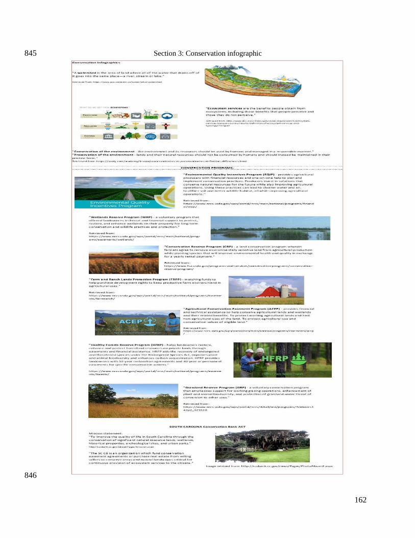
162
Section 3: Conservation infographic 845
846
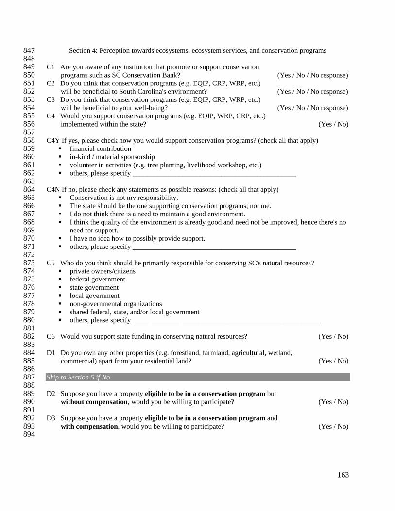
163
Section 4: Perception towards ecosystems, ecosystem services, and conservation programs 847 848 C1 Are you aware of any institution that promote or support conservation 849 programs such as SC Conservation Bank? (Yes / No / No response) 850 C2 Do you think that conservation programs (e.g. EQIP, CRP, WRP, etc.) 851 will be beneficial to South Carolina's environment? (Yes / No / No response) 852 C3 Do you think that conservation programs (e.g. EQIP, CRP, WRP, etc.) 853 will be beneficial to your well-being? (Yes / No / No response) 854 C4 Would you support conservation programs (e.g. EQIP, WRP, CRP, etc.) 855 implemented within the state? (Yes / No) 856 857 C4Y If yes, please check how you would support conservation programs? (check all that apply) 858
▪ financial contribution 859 ▪ in-kind / material sponsorship 860 ▪ volunteer in activities (e.g. tree planting, livelihood workshop, etc.) 861 ▪ others, please specify ______________________________________________ 862 863
C4N If no, please check any statements as possible reasons: (check all that apply) 864 ▪ Conservation is not my responsibility. 865 ▪ The state should be the one supporting conservation programs, not me. 866 ▪ I do not think there is a need to maintain a good environment. 867 ▪ I think the quality of the environment is already good and need not be improved, hence there's no 868
need for support. 869 ▪ I have no idea how to possibly provide support. 870 ▪ others, please specify ______________________________________________ 871
872 C5 Who do you think should be primarily responsible for conserving SC's natural resources? 873
▪ private owners/citizens 874 ▪ federal government 875 ▪ state government 876 ▪ local government 877 ▪ non-governmental organizations 878 ▪ shared federal, state, and/or local government 879 ▪ others, please specify ____________________________________________________ 880
881 C6 Would you support state funding in conserving natural resources? (Yes / No) 882 883 D1 Do you own any other properties (e.g. forestland, farmland, agricultural, wetland, 884 commercial) apart from your residential land? (Yes / No) 885 886 Skip to Section 5 if No 887 888 D2 Suppose you have a property eligible to be in a conservation program but 889 without compensation, would you be willing to participate? (Yes / No) 890 891 D3 Suppose you have a property eligible to be in a conservation program and 892 with compensation, would you be willing to participate? (Yes / No) 893 894

164
D4 In order to encourage more landowners to enter into conservation easement agreements, 895 how effective do you think the listed approaches will be? 896 897
Extremely
effective
Very
effective
Moderately
effective
Slightly
effective
Not
effective
at all
Financial incentives o o o o o Tax credits o o o o o
Opportunity to develop green
infrastructures o o o o o Opportunity to preserve the area o o o o o
Opportunity to contribute to better
environment o o o o o Opportunity to contribute to improvement
of society's welfare o o o o o 898 D5 Please write if you have other suggestions that you think would encourage land owners 899 to enter into conservation programs. 900
_________________________________________________________________________________ 901 902
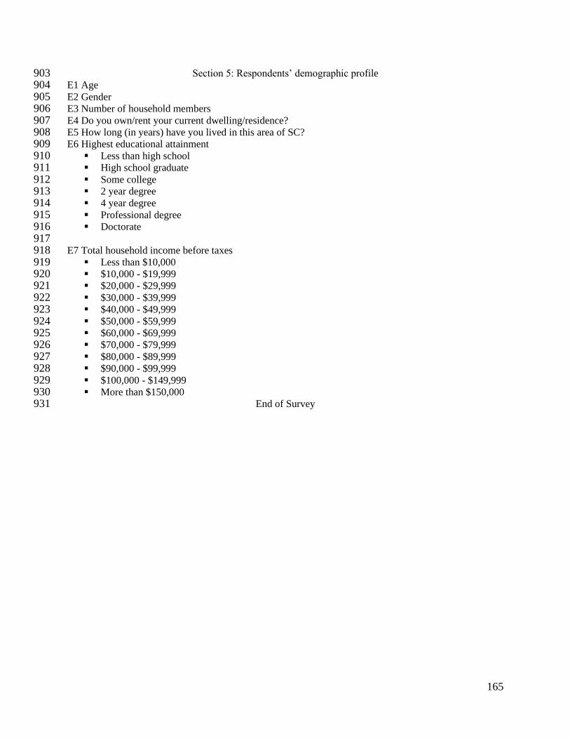
165
Section 5: Respondents’ demographic profile 903 E1 Age 904 E2 Gender 905 E3 Number of household members 906 E4 Do you own/rent your current dwelling/residence? 907 E5 How long (in years) have you lived in this area of SC? 908 E6 Highest educational attainment 909
▪ Less than high school 910 ▪ High school graduate 911 ▪ Some college 912 ▪ 2 year degree 913 ▪ 4 year degree 914 ▪ Professional degree 915 ▪ Doctorate 916
917 E7 Total household income before taxes 918
▪ Less than $10,000 919 ▪ $10,000 - $19,999 920 ▪ $20,000 - $29,999 921 ▪ $30,000 - $39,999 922 ▪ $40,000 - $49,999 923 ▪ $50,000 - $59,999 924 ▪ $60,000 - $69,999 925 ▪ $70,000 - $79,999 926 ▪ $80,000 - $89,999 927 ▪ $90,000 - $99,999 928 ▪ $100,000 - $149,999 929 ▪ More than $150,000 930
End of Survey 931

166
Appendix B 932
Summary statistics of residents' knowledge, awareness, and perceptions for conservation 933
Question Residents Landowners
N Yes % Yes N Yes % Yes
Are you aware about conservation programs (e.g.
EQIP, WRP, CRP, FRPP, ACEP, HFRP, GRP)? 1428 561 39% 228 157 69%
Environmental Quality Incentives Program (EQIP)
561
214 15%
157
19 12%
Wetlands Reserve Program (WRP) 398 28% 38 24%
Conservation Reserve Program (CRP) 262 18% 28 18%
Farm and Ranch Lands Protection Program (FRPP) 225 16% 24 15%
Agricultural Conservation Easement Program
(ACEP) 225 16% 23 15%
Healthy Forests Reserve Program (HFRP) 238 17% 21 13%
Grassland Reserve Program (GRP) 175 12% 12 8%
Are you aware of any institution that promote or
support conservation programs such as SC
Conservation Bank?
1428
476 33%
228
134 59%
Do you think that conservation programs will be
beneficial to SC's environment? 1232 86% 202 89%
Do you think that conservation programs will be
beneficial to your well-being? 1179 83% 185 81%
Perception that state should lead conservation 1283 90% 194 85%
Perception that public has a role in conservation 1313 92% 208 91%
Would you support conservation programs
implemented within the state? 1159 81% 196 86%
Yes: Financial contribution
1159
292 25%
Yes: in kind/material 142 12%
Yes: volunteer activities 890 77%
Yes: others 67 6%
No: Conservation is not my responsibility
269
30 11%
No: The state should support conservation
programs 49 18%
No: Don't think there's a need to maintain a good
environment 41 15%
No: No need to improve hence no need for support 30 11%
No: I have no idea how to support 139 52%
No: others 13 5%
Who do you think should be primarily responsible for
conserving SC's natural resources?
Private owners/citizens 1428
184 13% 228
59 26%
Federal government 76 5% 24 11%
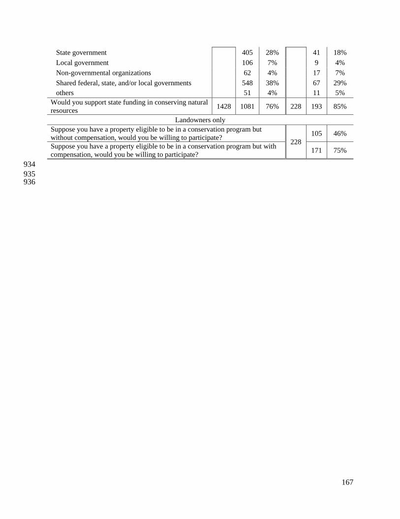
167
State government 405 28% 41 18%
Local government 106 7% 9 4%
Non-governmental organizations 62 4% 17 7%
Shared federal, state, and/or local governments 548 38% 67 29%
others 51 4% 11 5%
Would you support state funding in conserving natural
resources 1428 1081 76% 228 193 85%
Landowners only
Suppose you have a property eligible to be in a conservation program but
without compensation, would you be willing to participate? 228
105 46%
Suppose you have a property eligible to be in a conservation program but with
compensation, would you be willing to participate? 171 75%
934
935 936
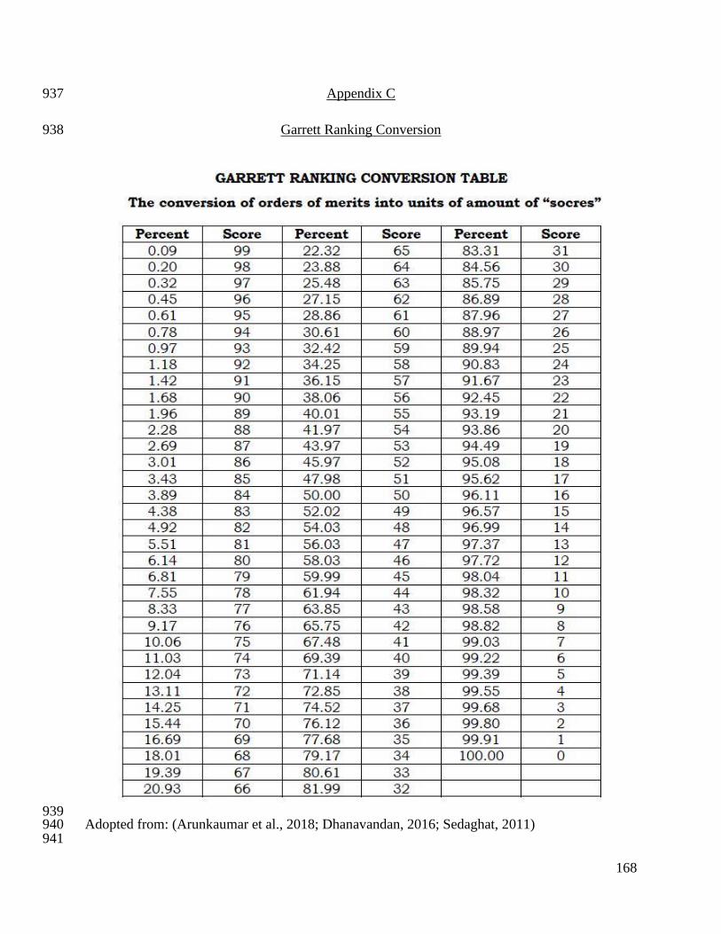
168
Appendix C 937
Garrett Ranking Conversion 938
939 Adopted from: (Arunkaumar et al., 2018; Dhanavandan, 2016; Sedaghat, 2011) 940 941
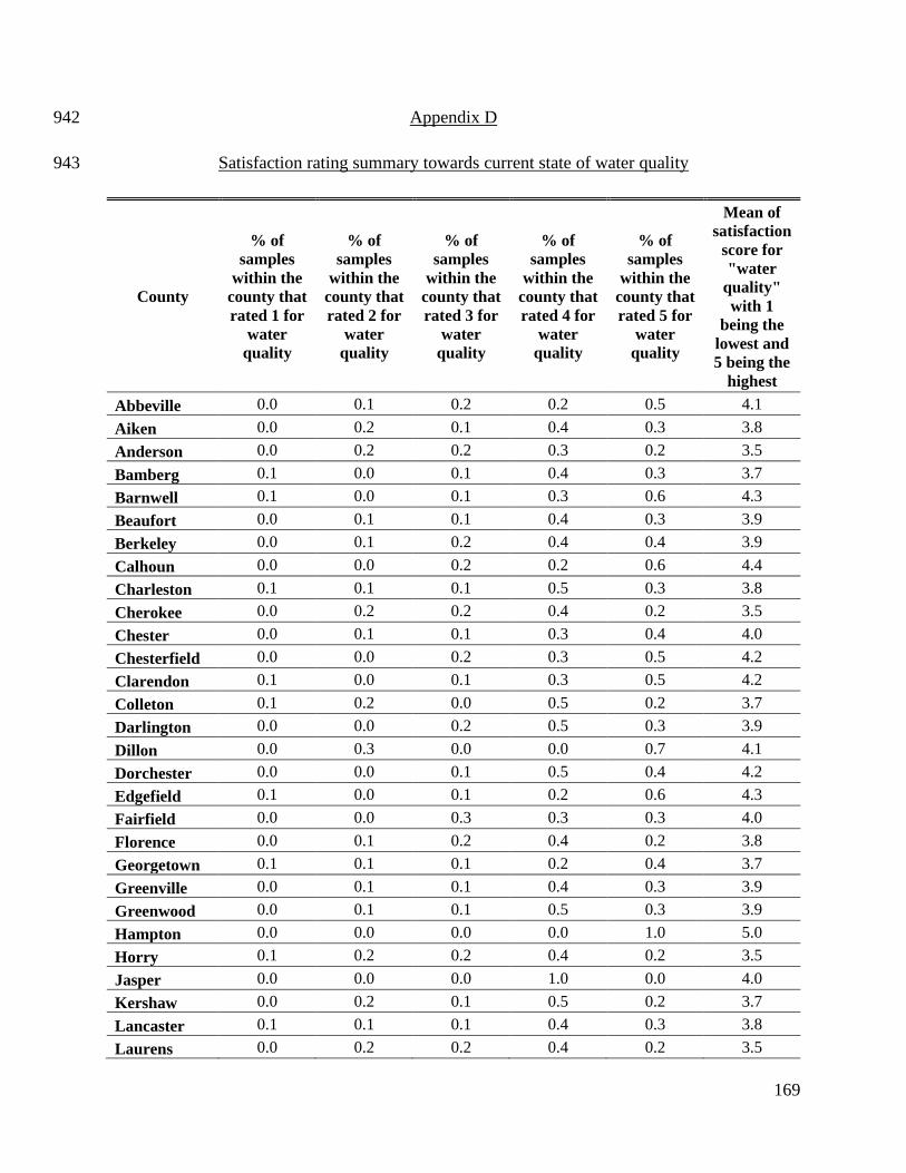
169
Appendix D 942
Satisfaction rating summary towards current state of water quality 943
County
% of
samples
within the
county that
rated 1 for
water
quality
% of
samples
within the
county that
rated 2 for
water
quality
% of
samples
within the
county that
rated 3 for
water
quality
% of
samples
within the
county that
rated 4 for
water
quality
% of
samples
within the
county that
rated 5 for
water
quality
Mean of
satisfaction
score for
"water
quality"
with 1
being the
lowest and
5 being the
highest
Abbeville 0.0 0.1 0.2 0.2 0.5 4.1
Aiken 0.0 0.2 0.1 0.4 0.3 3.8
Anderson 0.0 0.2 0.2 0.3 0.2 3.5
Bamberg 0.1 0.0 0.1 0.4 0.3 3.7
Barnwell 0.1 0.0 0.1 0.3 0.6 4.3
Beaufort 0.0 0.1 0.1 0.4 0.3 3.9
Berkeley 0.0 0.1 0.2 0.4 0.4 3.9
Calhoun 0.0 0.0 0.2 0.2 0.6 4.4
Charleston 0.1 0.1 0.1 0.5 0.3 3.8
Cherokee 0.0 0.2 0.2 0.4 0.2 3.5
Chester 0.0 0.1 0.1 0.3 0.4 4.0
Chesterfield 0.0 0.0 0.2 0.3 0.5 4.2
Clarendon 0.1 0.0 0.1 0.3 0.5 4.2
Colleton 0.1 0.2 0.0 0.5 0.2 3.7
Darlington 0.0 0.0 0.2 0.5 0.3 3.9
Dillon 0.0 0.3 0.0 0.0 0.7 4.1
Dorchester 0.0 0.0 0.1 0.5 0.4 4.2
Edgefield 0.1 0.0 0.1 0.2 0.6 4.3
Fairfield 0.0 0.0 0.3 0.3 0.3 4.0
Florence 0.0 0.1 0.2 0.4 0.2 3.8
Georgetown 0.1 0.1 0.1 0.2 0.4 3.7
Greenville 0.0 0.1 0.1 0.4 0.3 3.9
Greenwood 0.0 0.1 0.1 0.5 0.3 3.9
Hampton 0.0 0.0 0.0 0.0 1.0 5.0
Horry 0.1 0.2 0.2 0.4 0.2 3.5
Jasper 0.0 0.0 0.0 1.0 0.0 4.0
Kershaw 0.0 0.2 0.1 0.5 0.2 3.7
Lancaster 0.1 0.1 0.1 0.4 0.3 3.8
Laurens 0.0 0.2 0.2 0.4 0.2 3.5

170
Lee 0.0 0.0 0.0 0.3 0.7 4.7
Lexington 0.1 0.1 0.2 0.4 0.3 3.7
Marion 0.1 0.1 0.1 0.4 0.1 3.3
Marlboro 0.1 0.0 0.1 0.3 0.4 3.9
McCormick 0.1 0.0 0.0 0.7 0.2 3.9
Newberry 0.1 0.1 0.1 0.4 0.4 4.0
Oconee 0.0 0.2 0.1 0.5 0.3 3.9
Orangeburg 0.1 0.2 0.0 0.4 0.3 3.6
Pickens 0.0 0.1 0.2 0.4 0.3 3.9
Richland 0.0 0.1 0.1 0.5 0.3 4.0
Saluda 0.3 0.3 0.0 0.3 0.0 2.3
Spartanburg 0.0 0.1 0.2 0.4 0.3 3.8
Sumter 0.1 0.1 0.1 0.6 0.2 3.8
Union 0.0 0.0 0.0 1.0 0.0 4.0
Williamsburg 0.0 0.1 0.2 0.5 0.2 3.9
York 0.0 0.1 0.2 0.4 0.3 3.8
MEDIAN 3.9
944
945

171
Appendix E 946
Satisfaction rating summary towards current state of water supply 947
County
% of
samples
within the
county that
rated 1 for
water
supply
% of
samples
within the
county that
rated 2 for
water
supply
% of
samples
within the
county that
rated 3 for
water
supply
% of
samples
within the
county that
rated 4 for
water
supply
% of
samples
within the
county that
rated 5 for
water
supply
Mean of
satisfaction
score for
"water
supply"
with 1
being the
lowest and
5 being the
highest
Abbeville 0.0 0.1 0.1 0.3 0.5 4.2
Aiken 0.0 0.0 0.1 0.3 0.6 4.4
Anderson 0.0 0.0 0.1 0.4 0.5 4.3
Bamberg 0.1 0.0 0.1 0.3 0.4 3.9
Barnwell 0.0 0.1 0.2 0.3 0.5 4.2
Beaufort 0.0 0.0 0.1 0.2 0.7 4.5
Berkeley 0.0 0.0 0.0 0.3 0.6 4.4
Calhoun 0.0 0.0 0.0 0.4 0.6 4.6
Charleston 0.0 0.0 0.1 0.2 0.6 4.3
Cherokee 0.0 0.1 0.1 0.2 0.6 4.3
Chester 0.0 0.0 0.1 0.6 0.4 4.3
Chesterfield 0.0 0.0 0.1 0.2 0.7 4.5
Clarendon 0.0 0.0 0.1 0.4 0.5 4.4
Colleton 0.1 0.0 0.1 0.2 0.6 4.3
Darlington 0.0 0.0 0.1 0.4 0.4 4.2
Dillon 0.0 0.0 0.3 0.3 0.4 4.1
Dorchester 0.0 0.0 0.1 0.2 0.7 4.6
Edgefield 0.0 0.1 0.0 0.1 0.8 4.6
Fairfield 0.0 0.3 0.0 0.3 0.3 3.7
Florence 0.0 0.1 0.1 0.4 0.5 4.2
Georgetown 0.0 0.0 0.1 0.2 0.7 4.6
Greenville 0.0 0.0 0.1 0.3 0.5 4.3
Greenwood 0.0 0.0 0.1 0.3 0.6 4.6
Hampton 0.0 0.0 0.0 0.0 1.0 5.0
Horry 0.0 0.0 0.1 0.2 0.6 4.3
Jasper 0.0 0.0 0.0 0.6 0.4 4.4
Kershaw 0.0 0.0 0.0 0.3 0.7 4.6
Lancaster 0.1 0.0 0.1 0.2 0.6 4.2
Laurens 0.0 0.0 0.2 0.2 0.6 4.2

172
Lee 0.0 0.0 0.0 0.3 0.7 4.7
Lexington 0.0 0.0 0.1 0.4 0.5 4.2
Marion 0.0 0.0 0.1 0.4 0.4 4.3
Marlboro 0.1 0.0 0.1 0.4 0.3 3.7
McCormick 0.0 0.0 0.0 0.5 0.5 4.5
Newberry 0.1 0.1 0.3 0.2 0.4 3.8
Oconee 0.0 0.1 0.0 0.2 0.7 4.5
Orangeburg 0.0 0.1 0.1 0.3 0.5 4.2
Pickens 0.0 0.0 0.1 0.2 0.7 4.7
Richland 0.0 0.0 0.2 0.2 0.6 4.4
Saluda 0.0 0.3 0.0 0.3 0.3 3.7
Spartanburg 0.0 0.0 0.1 0.2 0.6 4.4
Sumter 0.0 0.0 0.1 0.5 0.4 4.2
Union 0.0 0.0 0.0 0.2 0.8 4.8
Williamsburg 0.0 0.1 0.2 0.3 0.4 4.1
York 0.0 0.1 0.2 0.3 0.5 4.2
MEDIAN 4.3
948
949
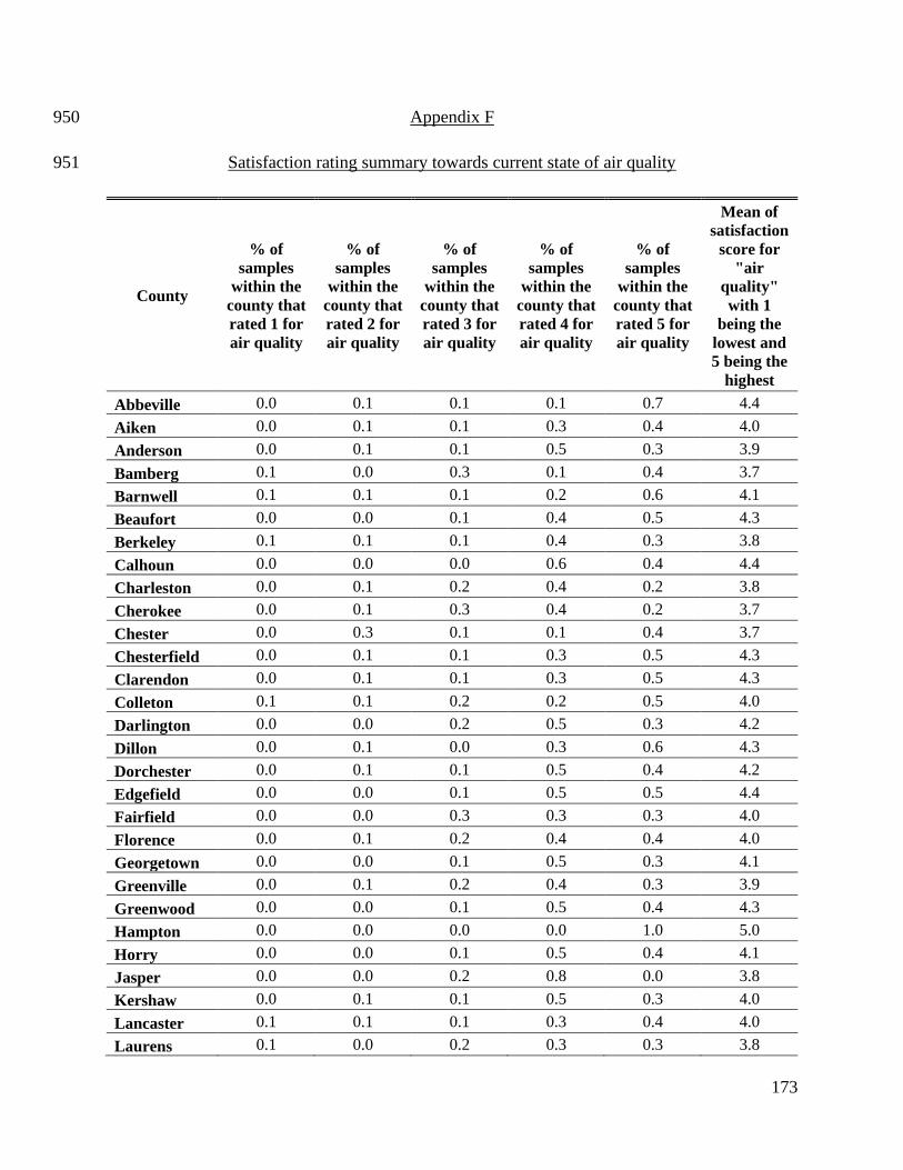
173
Appendix F 950
Satisfaction rating summary towards current state of air quality 951
County
% of
samples
within the
county that
rated 1 for
air quality
% of
samples
within the
county that
rated 2 for
air quality
% of
samples
within the
county that
rated 3 for
air quality
% of
samples
within the
county that
rated 4 for
air quality
% of
samples
within the
county that
rated 5 for
air quality
Mean of
satisfaction
score for
"air
quality"
with 1
being the
lowest and
5 being the
highest
Abbeville 0.0 0.1 0.1 0.1 0.7 4.4
Aiken 0.0 0.1 0.1 0.3 0.4 4.0
Anderson 0.0 0.1 0.1 0.5 0.3 3.9
Bamberg 0.1 0.0 0.3 0.1 0.4 3.7
Barnwell 0.1 0.1 0.1 0.2 0.6 4.1
Beaufort 0.0 0.0 0.1 0.4 0.5 4.3
Berkeley 0.1 0.1 0.1 0.4 0.3 3.8
Calhoun 0.0 0.0 0.0 0.6 0.4 4.4
Charleston 0.0 0.1 0.2 0.4 0.2 3.8
Cherokee 0.0 0.1 0.3 0.4 0.2 3.7
Chester 0.0 0.3 0.1 0.1 0.4 3.7
Chesterfield 0.0 0.1 0.1 0.3 0.5 4.3
Clarendon 0.0 0.1 0.1 0.3 0.5 4.3
Colleton 0.1 0.1 0.2 0.2 0.5 4.0
Darlington 0.0 0.0 0.2 0.5 0.3 4.2
Dillon 0.0 0.1 0.0 0.3 0.6 4.3
Dorchester 0.0 0.1 0.1 0.5 0.4 4.2
Edgefield 0.0 0.0 0.1 0.5 0.5 4.4
Fairfield 0.0 0.0 0.3 0.3 0.3 4.0
Florence 0.0 0.1 0.2 0.4 0.4 4.0
Georgetown 0.0 0.0 0.1 0.5 0.3 4.1
Greenville 0.0 0.1 0.2 0.4 0.3 3.9
Greenwood 0.0 0.0 0.1 0.5 0.4 4.3
Hampton 0.0 0.0 0.0 0.0 1.0 5.0
Horry 0.0 0.0 0.1 0.5 0.4 4.1
Jasper 0.0 0.0 0.2 0.8 0.0 3.8
Kershaw 0.0 0.1 0.1 0.5 0.3 4.0
Lancaster 0.1 0.1 0.1 0.3 0.4 4.0
Laurens 0.1 0.0 0.2 0.3 0.3 3.8
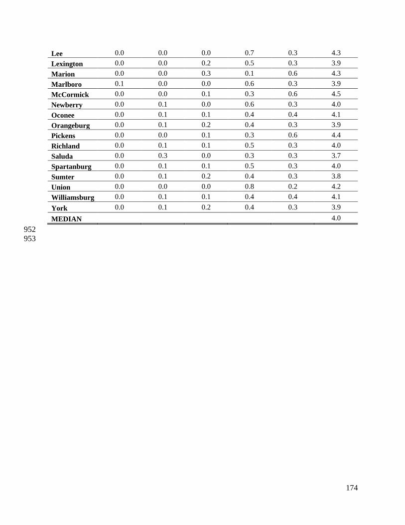
174
Lee 0.0 0.0 0.0 0.7 0.3 4.3
Lexington 0.0 0.0 0.2 0.5 0.3 3.9
Marion 0.0 0.0 0.3 0.1 0.6 4.3
Marlboro 0.1 0.0 0.0 0.6 0.3 3.9
McCormick 0.0 0.0 0.1 0.3 0.6 4.5
Newberry 0.0 0.1 0.0 0.6 0.3 4.0
Oconee 0.0 0.1 0.1 0.4 0.4 4.1
Orangeburg 0.0 0.1 0.2 0.4 0.3 3.9
Pickens 0.0 0.0 0.1 0.3 0.6 4.4
Richland 0.0 0.1 0.1 0.5 0.3 4.0
Saluda 0.0 0.3 0.0 0.3 0.3 3.7
Spartanburg 0.0 0.1 0.1 0.5 0.3 4.0
Sumter 0.0 0.1 0.2 0.4 0.3 3.8
Union 0.0 0.0 0.0 0.8 0.2 4.2
Williamsburg 0.0 0.1 0.1 0.4 0.4 4.1
York 0.0 0.1 0.2 0.4 0.3 3.9
MEDIAN 4.0
952
953

175
Appendix G 954
Satisfaction rating summary towards current state of the overall environment 955
County
% of
samples
within the
county that
rated 1 for
overall
state of the
environme
nt
% of
samples
within the
county that
rated 2 for
overall
state of the
environme
nt
% of
samples
within the
county that
rated 3 for
overall
state of the
environme
nt
% of
samples
within the
county that
rated 4 for
overall
state of the
environme
nt
% of
samples
within the
county that
rated 5 for
overall
state of the
environme
nt
Mean of
satisfaction
score for
"overall
state of the
environment
" with 1
being the
lowest and 5
being the
highest
Abbeville 0.1 0.0 0.1 0.3 0.5 4.1
Aiken 0.1 0.1 0.2 0.3 0.3 3.8
Anderson 0.0 0.1 0.2 0.5 0.1 3.6
Bamberg 0.1 0.0 0.3 0.1 0.4 3.7
Barnwell 0.0 0.1 0.1 0.3 0.5 4.3
Beaufort 0.0 0.0 0.1 0.6 0.3 4.1
Berkeley 0.0 0.1 0.3 0.3 0.2 3.6
Calhoun 0.0 0.0 0.2 0.6 0.2 4.0
Charleston 0.0 0.1 0.2 0.4 0.1 3.5
Cherokee 0.0 0.2 0.2 0.4 0.2 3.5
Chester 0.1 0.3 0.1 0.4 0.1 3.3
Chesterfield 0.0 0.1 0.1 0.4 0.5 4.1
Clarendon 0.0 0.3 0.1 0.5 0.2 3.6
Colleton 0.1 0.2 0.1 0.3 0.4 3.8
Darlington 0.0 0.2 0.2 0.4 0.3 3.7
Dillon 0.0 0.3 0.1 0.1 0.4 3.7
Dorchester 0.0 0.1 0.1 0.5 0.3 4.0
Edgefield 0.0 0.0 0.3 0.5 0.3 4.0
Fairfield 0.0 0.0 0.3 0.3 0.3 4.0
Florence 0.0 0.1 0.2 0.4 0.2 3.7
Georgetown 0.0 0.1 0.2 0.4 0.3 3.9
Greenville 0.0 0.1 0.2 0.5 0.2 3.8
Greenwood 0.0 0.1 0.2 0.5 0.3 4.0
Hampton 0.0 0.0 0.0 0.0 1.0 5.0
Horry 0.0 0.1 0.2 0.5 0.2 3.7
Jasper 0.0 0.0 0.4 0.6 0.0 3.6
Kershaw 0.0 0.3 0.0 0.5 0.2 3.5
Lancaster 0.0 0.1 0.1 0.5 0.3 3.9
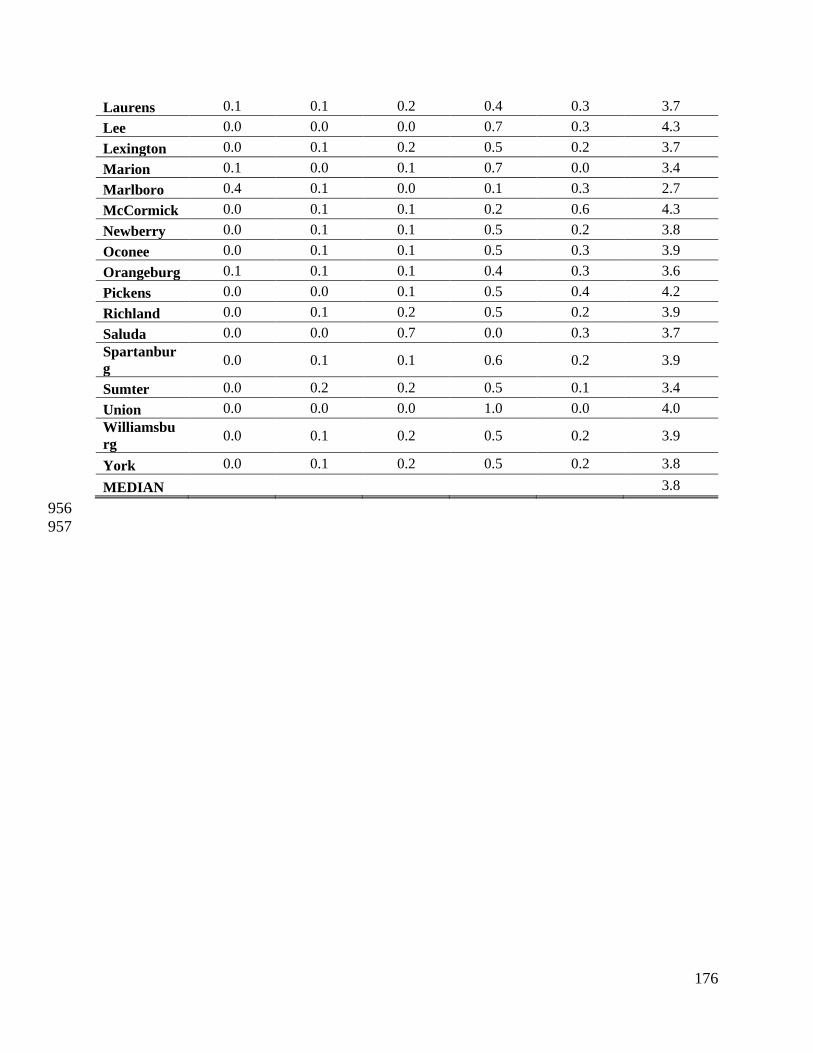
176
Laurens 0.1 0.1 0.2 0.4 0.3 3.7
Lee 0.0 0.0 0.0 0.7 0.3 4.3
Lexington 0.0 0.1 0.2 0.5 0.2 3.7
Marion 0.1 0.0 0.1 0.7 0.0 3.4
Marlboro 0.4 0.1 0.0 0.1 0.3 2.7
McCormick 0.0 0.1 0.1 0.2 0.6 4.3
Newberry 0.0 0.1 0.1 0.5 0.2 3.8
Oconee 0.0 0.1 0.1 0.5 0.3 3.9
Orangeburg 0.1 0.1 0.1 0.4 0.3 3.6
Pickens 0.0 0.0 0.1 0.5 0.4 4.2
Richland 0.0 0.1 0.2 0.5 0.2 3.9
Saluda 0.0 0.0 0.7 0.0 0.3 3.7
Spartanbur
g 0.0 0.1 0.1 0.6 0.2 3.9
Sumter 0.0 0.2 0.2 0.5 0.1 3.4
Union 0.0 0.0 0.0 1.0 0.0 4.0
Williamsbu
rg 0.0 0.1 0.2 0.5 0.2 3.9
York 0.0 0.1 0.2 0.5 0.2 3.8
MEDIAN 3.8
956
957
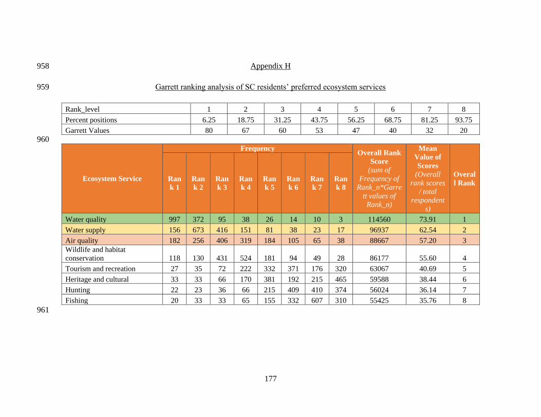
177
Appendix H 958
Garrett ranking analysis of SC residents’ preferred ecosystem services 959
Rank_level 1 2 3 4 5 6 7 8
Percent positions 6.25 18.75 31.25 43.75 56.25 68.75 81.25 93.75
Garrett Values 80 67 60 53 47 40 32 20
960
Ecosystem Service
Frequency Overall Rank
Score
(sum of
Frequency of
Rank_n*Garre
tt values of
Rank_n)
Mean
Value of
Scores
(Overall
rank scores
/ total
respondent
s)
Overal
l Rank Ran
k 1
Ran
k 2
Ran
k 3
Ran
k 4
Ran
k 5
Ran
k 6
Ran
k 7
Ran
k 8
Water quality 997 372 95 38 26 14 10 3 114560 73.91 1
Water supply 156 673 416 151 81 38 23 17 96937 62.54 2
Air quality 182 256 406 319 184 105 65 38 88667 57.20 3
Wildlife and habitat
conservation 118 130 431 524 181 94 49 28 86177 55.60 4
Tourism and recreation 27 35 72 222 332 371 176 320 63067 40.69 5
Heritage and cultural 33 33 66 170 381 192 215 465 59588 38.44 6
Hunting 22 23 36 66 215 409 410 374 56024 36.14 7
Fishing 20 33 33 65 155 332 607 310 55425 35.76 8
961
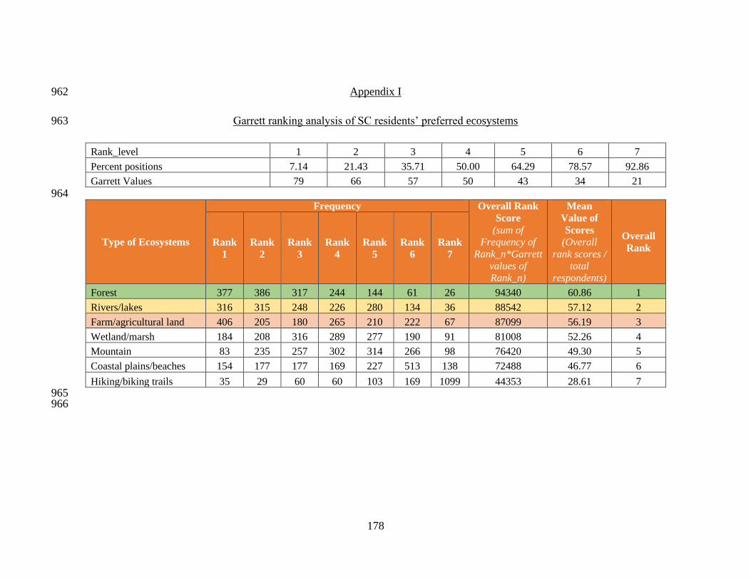
178
Appendix I 962
Garrett ranking analysis of SC residents’ preferred ecosystems 963
Rank_level 1 2 3 4 5 6 7
Percent positions 7.14 21.43 35.71 50.00 64.29 78.57 92.86
Garrett Values 79 66 57 50 43 34 21
964
Type of Ecosystems
Frequency Overall Rank
Score
(sum of
Frequency of
Rank_n*Garrett
values of
Rank_n)
Mean
Value of
Scores
(Overall
rank scores /
total
respondents)
Overall
Rank Rank
1
Rank
2
Rank
3
Rank
4
Rank
5
Rank
6
Rank
7
Forest 377 386 317 244 144 61 26 94340 60.86 1
Rivers/lakes 316 315 248 226 280 134 36 88542 57.12 2
Farm/agricultural land 406 205 180 265 210 222 67 87099 56.19 3
Wetland/marsh 184 208 316 289 277 190 91 81008 52.26 4
Mountain 83 235 257 302 314 266 98 76420 49.30 5
Coastal plains/beaches 154 177 177 169 227 513 138 72488 46.77 6
Hiking/biking trails 35 29 60 60 103 169 1099 44353 28.61 7 965 966

179
Appendix J 967
Mean sediment retention capacity by landcover with and without cover crops 968
Land Cover
(tons/acre)
Jan Feb Mar Apr May Jun
No
cover
crops
With
cover
crops
No
cover
crops
With
cover
crops
No
cover
crops
With
cover
crops
No
cover
crops
With
cover
crops
No
cover
crops
With
cover
crops
No
cover
crops
With
cover
crops
Water 1.7 1.7 1.9 1.9 1.7 1.7 2.1 2.1 1.3 1.3 1.4 1.4
Shrubland 5.6 5.6 6.4 6.4 5.8 5.8 7.0 7.0 4.3 4.3 4.5 4.5
Herbaceous Wetland 0.6 0.6 0.8 0.8 0.7 0.7 0.8 0.8 0.5 0.5 0.6 0.6
Woody Wetland 2.5 2.5 3.1 3.1 2.6 2.6 3.2 3.2 1.9 1.9 2.3 2.3
Forest 18.4 18.3 19.6 19.6 18.0 18.0 21.8 21.8 14.3 14.3 14.5 14.5
Grassland/Pasture 8.5 8.5 9.2 9.2 8.4 8.4 10.3 10.3 6.6 6.6 6.6 6.6
Idle Cropland 2.8 2.9 3.3 3.3 2.9 3.0 3.6 3.6 2.2 2.2 2.4 2.4
Barren 8.9 9.1 9.8 9.8 9.0 9.0 10.8 10.8 6.9 6.9 7.0 7.0
Developed/Urban 6.4 6.7 6.7 6.7 6.2 6.2 7.6 7.6 5.0 5.0 5.0 5.0
Agriculture 3.3 3.2 0.1 2.1 0.0 1.8 0.1 2.1 0.1 2.2 0.1 2.3
Offseason cropland 2.7 2.8 3.9 4.2 3.6 3.9 5.7 6.1 1.9 2.0 0.7 0.7
Land Cover
(tons/acre)
Jul Aug Sep Oct Nov Dec
No
cover
crops
With
cover
crops
No
cover
crops
With
cover
crops
No
cover
crops
With
cover
crops
No
cover
crops
With
cover
crops
No
cover
crops
With
cover
crops
No
cover
crops
With
cover
crops
Water 2.1 2.1 2.2 2.2 2.4 2.4 1.7 1.7 1.6 1.6 1.4 1.4
Shrubland 7.4 7.4 7.5 7.5 8.2 8.2 5.8 5.8 5.2 5.2 4.7 4.7
Herbaceous Wetland 1.1 1.1 1.2 1.2 1.4 1.4 1.0 1.0 0.7 0.7 0.5 0.5
Woody Wetland 4.3 4.3 4.4 4.4 5.0 5.0 3.1 3.1 2.5 2.5 2.0 2.0
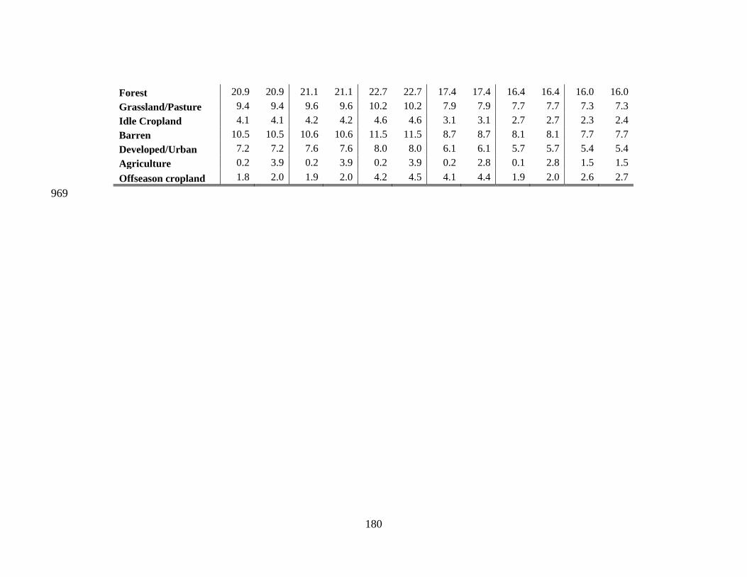
180
Forest 20.9 20.9 21.1 21.1 22.7 22.7 17.4 17.4 16.4 16.4 16.0 16.0
Grassland/Pasture 9.4 9.4 9.6 9.6 10.2 10.2 7.9 7.9 7.7 7.7 7.3 7.3
Idle Cropland 4.1 4.1 4.2 4.2 4.6 4.6 3.1 3.1 2.7 2.7 2.3 2.4
Barren 10.5 10.5 10.6 10.6 11.5 11.5 8.7 8.7 8.1 8.1 7.7 7.7
Developed/Urban 7.2 7.2 7.6 7.6 8.0 8.0 6.1 6.1 5.7 5.7 5.4 5.4
Agriculture 0.2 3.9 0.2 3.9 0.2 3.9 0.2 2.8 0.1 2.8 1.5 1.5
Offseason cropland 1.8 2.0 1.9 2.0 4.2 4.5 4.1 4.4 1.9 2.0 2.6 2.7
969
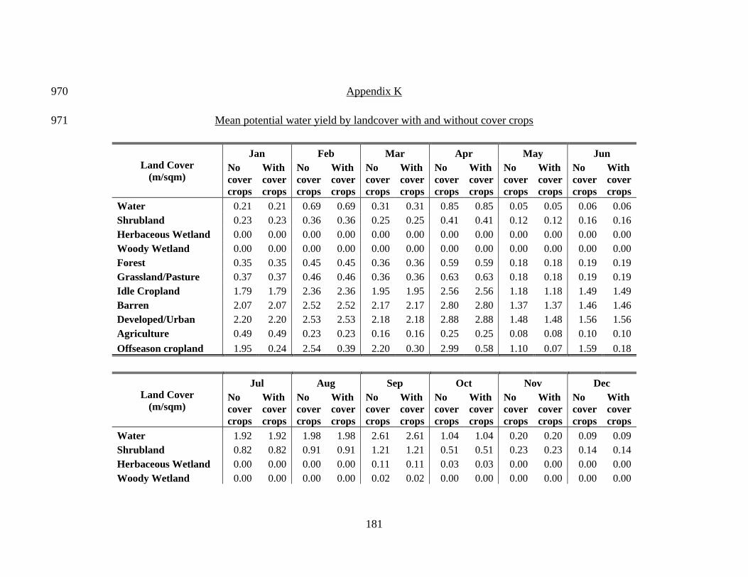
181
Appendix K 970
Mean potential water yield by landcover with and without cover crops 971
Land Cover
(m/sqm)
Jan Feb Mar Apr May Jun
No
cover
crops
With
cover
crops
No
cover
crops
With
cover
crops
No
cover
crops
With
cover
crops
No
cover
crops
With
cover
crops
No
cover
crops
With
cover
crops
No
cover
crops
With
cover
crops
Water 0.21 0.21 0.69 0.69 0.31 0.31 0.85 0.85 0.05 0.05 0.06 0.06
Shrubland 0.23 0.23 0.36 0.36 0.25 0.25 0.41 0.41 0.12 0.12 0.16 0.16
Herbaceous Wetland 0.00 0.00 0.00 0.00 0.00 0.00 0.00 0.00 0.00 0.00 0.00 0.00
Woody Wetland 0.00 0.00 0.00 0.00 0.00 0.00 0.00 0.00 0.00 0.00 0.00 0.00
Forest 0.35 0.35 0.45 0.45 0.36 0.36 0.59 0.59 0.18 0.18 0.19 0.19
Grassland/Pasture 0.37 0.37 0.46 0.46 0.36 0.36 0.63 0.63 0.18 0.18 0.19 0.19
Idle Cropland 1.79 1.79 2.36 2.36 1.95 1.95 2.56 2.56 1.18 1.18 1.49 1.49
Barren 2.07 2.07 2.52 2.52 2.17 2.17 2.80 2.80 1.37 1.37 1.46 1.46
Developed/Urban 2.20 2.20 2.53 2.53 2.18 2.18 2.88 2.88 1.48 1.48 1.56 1.56
Agriculture 0.49 0.49 0.23 0.23 0.16 0.16 0.25 0.25 0.08 0.08 0.10 0.10
Offseason cropland 1.95 0.24 2.54 0.39 2.20 0.30 2.99 0.58 1.10 0.07 1.59 0.18
Land Cover
(m/sqm)
Jul Aug Sep Oct Nov Dec
No
cover
crops
With
cover
crops
No
cover
crops
With
cover
crops
No
cover
crops
With
cover
crops
No
cover
crops
With
cover
crops
No
cover
crops
With
cover
crops
No
cover
crops
With
cover
crops
Water 1.92 1.92 1.98 1.98 2.61 2.61 1.04 1.04 0.20 0.20 0.09 0.09
Shrubland 0.82 0.82 0.91 0.91 1.21 1.21 0.51 0.51 0.23 0.23 0.14 0.14
Herbaceous Wetland 0.00 0.00 0.00 0.00 0.11 0.11 0.03 0.03 0.00 0.00 0.00 0.00
Woody Wetland 0.00 0.00 0.00 0.00 0.02 0.02 0.00 0.00 0.00 0.00 0.00 0.00
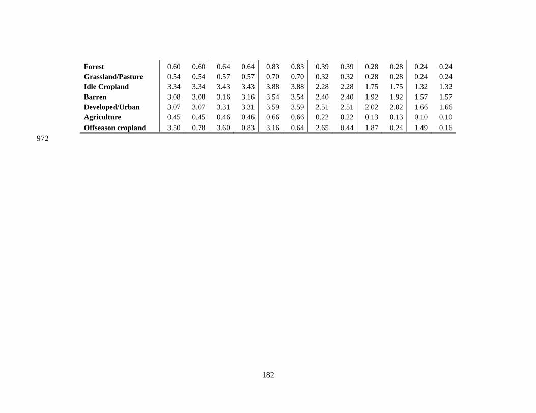
182
Forest 0.60 0.60 0.64 0.64 0.83 0.83 0.39 0.39 0.28 0.28 0.24 0.24
Grassland/Pasture 0.54 0.54 0.57 0.57 0.70 0.70 0.32 0.32 0.28 0.28 0.24 0.24
Idle Cropland 3.34 3.34 3.43 3.43 3.88 3.88 2.28 2.28 1.75 1.75 1.32 1.32
Barren 3.08 3.08 3.16 3.16 3.54 3.54 2.40 2.40 1.92 1.92 1.57 1.57
Developed/Urban 3.07 3.07 3.31 3.31 3.59 3.59 2.51 2.51 2.02 2.02 1.66 1.66
Agriculture 0.45 0.45 0.46 0.46 0.66 0.66 0.22 0.22 0.13 0.13 0.10 0.10
Offseason cropland 3.50 0.78 3.60 0.83 3.16 0.64 2.65 0.44 1.87 0.24 1.49 0.16
972

183
Appendix L 973
Choice experiment survey questionnaire for eliciting respondents’ willingness to pay 974
Eliciting Residents' Choices Towards Ecosystem Services Improvement 975 976
Introduction 977 978
You have been randomly selected to participate in a survey being conducted by researchers from the 979 Baruch Institute of Coastal Ecology and Forest Science at Clemson University. 980 981 You will be asked to read information, watch video clips, and respond to questions on your perception 982 and position pertaining to environmental and resource conservation and activities. This study aims to 983 understand the value on which stakeholders place on the environment through its ecosystem services. In 984 this manner, policies towards prioritization between development and conservation can be developed 985 simultaneously while maintaining sustainability of resources in SC. Therefore, we are gathering 986 information from SC residents as primary stakeholders to have a deeper understanding of the residents’ 987 view point. 988 989 Your participation in the interview will be VOLUNTARY and will take approximately 20-25 minutes. 990 Your refusal to participate in or to withdraw from the study carries no penalty or loss of any benefits. The 991 information that you provide will be kept CONFIDENTIAL and will not be released to any other entity 992 that is not involved in the study. No one will know your answers but our research team, and your identity 993 will be protected in any report based on the data. 994 995 Please bear in mind that, although this is merely a research study and the propositions presented are 996 hypothetical, your participation in the survey is critical and the results could be used as basis to further 997 improve sustainable development policies of our natural resources. We hope you can help us by 998 participating in this survey. If you do agree to participate in this survey, please answer the questions as 999 best and truthful as you can. If you are willing to participate, please proceed to the succeeding questions. 1000 1001 We care about the quality of our survey data and hope to receive the most accurate measures of your 1002 opinions, so it is important to us that you thoughtfully provide your best answer to each question in the 1003 survey. 1004 1005 Do you commit to providing your thoughtful and honest answers to the questions in this survey? 1006
a. I will provide my best answers 1007 b. I will not provide my best answers 1008 c. I can't promise either way 1009
Do you currently live in South Carolina? (Yes / No) 1010 What county do you live in? 1011 What city/town do you live in? 1012 Are you completing this survey within the vicinity of your residence? (Yes / No) 1013 Are you the "finance decision maker" of your household? (Yes / No) 1014 (finance decision maker - the one who controls the household budget 1015 and decides prioritization of regular household expenditure) 1016
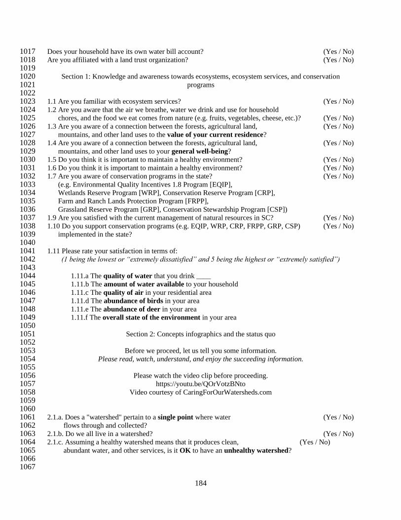
184
Does your household have its own water bill account? (Yes / No) 1017 Are you affiliated with a land trust organization? (Yes / No) 1018 1019
Section 1: Knowledge and awareness towards ecosystems, ecosystem services, and conservation 1020 programs 1021
1022 1.1 Are you familiar with ecosystem services? (Yes / No) 1023 1.2 Are you aware that the air we breathe, water we drink and use for household 1024 chores, and the food we eat comes from nature (e.g. fruits, vegetables, cheese, etc.)? (Yes / No) 1025 1.3 Are you aware of a connection between the forests, agricultural land, (Yes / No) 1026 mountains, and other land uses to the value of your current residence? 1027 1.4 Are you aware of a connection between the forests, agricultural land, (Yes / No) 1028 mountains, and other land uses to your general well-being? 1029 1.5 Do you think it is important to maintain a healthy environment? (Yes / No) 1030 1.6 Do you think it is important to maintain a healthy environment? (Yes / No) 1031 1.7 Are you aware of conservation programs in the state? (Yes / No) 1032 (e.g. Environmental Quality Incentives 1.8 Program [EQIP], 1033 Wetlands Reserve Program [WRP], Conservation Reserve Program [CRP], 1034 Farm and Ranch Lands Protection Program [FRPP], 1035 Grassland Reserve Program [GRP], Conservation Stewardship Program [CSP]) 1036 1.9 Are you satisfied with the current management of natural resources in SC? (Yes / No) 1037 1.10 Do you support conservation programs (e.g. EQIP, WRP, CRP, FRPP, GRP, CSP) (Yes / No) 1038 implemented in the state? 1039 1040 1.11 Please rate your satisfaction in terms of: 1041
(1 being the lowest or “extremely dissatisfied” and 5 being the highest or “extremely satisfied”) 1042 1043
1.11.a The quality of water that you drink ____ 1044 1.11.b The amount of water available to your household 1045 1.11.c The quality of air in your residential area 1046 1.11.d The abundance of birds in your area 1047 1.11.e The abundance of deer in your area 1048 1.11.f The overall state of the environment in your area 1049 1050
Section 2: Concepts infographics and the status quo 1051 1052
Before we proceed, let us tell you some information. 1053 Please read, watch, understand, and enjoy the succeeding information. 1054
1055 Please watch the video clip before proceeding. 1056
https://youtu.be/QOrVotzBNto 1057 Video courtesy of CaringForOurWatersheds.com 1058
1059 1060
2.1.a. Does a "watershed" pertain to a single point where water (Yes / No) 1061 flows through and collected? 1062 2.1.b. Do we all live in a watershed? (Yes / No) 1063 2.1.c. Assuming a healthy watershed means that it produces clean, (Yes / No) 1064 abundant water, and other services, is it OK to have an unhealthy watershed? 1065
1066 1067

185
Please watch the videoclip before proceeding. 1068 https://youtu.be/V_FQ2cpHNGw 1069
Video courtesy of Clemson University Motallebi’s lab 1070 1071 2.2.a. Do you agree with the statement that "Ecosystem services are benefits that (Yes / No) 1072 we get from nature"? 1073 2.2.b. Are recreational and spiritual benefits part of ecosystem services? (Yes / No) 1074 2.2.c. How much amount do we pay to the ecosystem in exchange for its services? 1075 a. more than $1000.00 (A great deal) 1076
b. $151.00 - $1000.00 (A lot) 1077 c. $51.00 - $150.00 (A moderate amount) 1078 d. $1.00 - $50.00 (A little) 1079 e. $0.00 (None at all) 1080
1081 (Please read the infographics thoroughly) 1082
1083 South Carolina is composed of 4 major River-Basin networks (Savannah, Edisto-Salkehatchie, Santee, 1084 Pee Dee), which was further subdivided into 8 major Basins. These 8 basins hold numerous 1085 interconnected network of sub-basins and watersheds which provide ecosystem services to its residents. 1086 1087
1088 1089 Similar to all other sub-basins in South Carolina, Congaree and Wateree Sub-basins are key ecosystems 1090 which provide ecosystem services to the state. Apart from the commonly known provisioning ecosystem 1091 services (i.e. agricultural produce, hydropower energy, water, etc.) which contribute to economic 1092 progress, it also maintains the quality of ecosystem services (i.e. clean air and water, healthy habitat for 1093 wildlife, etc.) and ensures that these are continuously provided for the benefit of the stakeholders. 1094 1095 For instance, in terms of water supply, an ecosystem-based model estimated that the 178,000 hectare 1096 (440,000 acres) Congaree sub-basin contributes around 303 million cubic meter of water (average of 1097 1,700 cu meter per hectare of land) annually to the streams which stakeholders can use for daily 1098

186
activities. However, with the current land uses in the sub-basin, water quality is also affected through 1099 11 million tons of sediments exported ( average of 65.32 tons per hectare) to the streams annually. 1100 1101 With social and economic pressures of urbanization growing (e.g. population growth, increasing needs 1102 and wants, economic expansions, etc.), a trade-off of prioritization of land uses between 1103 environmental/agricultural use and economic development is at hand. 1104 1105 Although economic development certainly has benefits to the welfare of the stakeholders, the change of 1106 the land uses favoring urbanization, more often, also affects the ecosystem services negatively. This could 1107 possibly entail reduction of water contributed by the basin to the streams, as well increased sediments 1108 being exported to the streams and river, hence affecting water quality negatively. 1109 1110 From 2006 to 2011 in Congaree sub-basin alone, approximately 130 hectares of forested land and 1111 around 50 hectares of agricultural land were converted due to urbanization. Similarly, other land uses 1112 have also been affected while being converted to urban areas. 1113 1114
1115 1116
To further understand the effect of urbanization, a land cover projection of increased urbanized areas were 1117 conducted for the Congaree sub-basin. This projection was run with a scenario considering that the 1118 current activities in the sub-basin will continue "as usual" until 2030, hence we call it the "Status 1119 Quo". 1120

187
1121 1122 The result of the model showed that given the Status Quo, the amount of water being contributed to the 1123 stream will increase by 4% (315 million cubic meters or 1,770 cubic meter per hectare), however the 1124 amount of sediments that will be exported to the streams will also increase by 3% (11.7 million tons 1125 or 65.32 tons per hectare). This means that, although there will still be more water available, the 1126 quality of water that stakeholders use will be affected negatively. 1127 1128 Furthermore, the projected urbanization will also have negative results to wildlife habitat, particularly a 5-1129 10% loss of habitat potentially for bobwhite quails, dears, and song birds. These wildlife species play 1130 significant roles for recreational, traditional, and socio-cultural values particularly in South Carolina. 1131 1132 To address the issue of urbanization, since most of the urban areas were previously agricultural or forest 1133 land uses, it is imperative to encourage farmers and land owners to maintain or enhance farms or forest 1134 lands. One way to encourage farmers and land owners is through incentives from retaining the land 1135 as farm or forested area. This means employing sustainable management practices in agricultural and 1136 forest lands (i.e. cover crops and agroforestry implementation). 1137 1138
Information about cover crop farming 1139 Please watch the videoclip before proceeding... 1140
https://youtu.be/3j5MRJeCoYs 1141 Video courtesy of Natural Resource Defense Council, Inc. 1142
1143 Information about agroforestry farming 1144
Please watch the videoclip before proceeding... 1145 https://youtu.be/MZ6No1mL1QM 1146
Video courtesy of RUVIVAL.hoou.de (www.ruvival.de) 1147 1148

188
Utilizing these methods as means for conservation and sustainable farming practice can substantially 1149 improve the state of the ecosystem, ecosystem services, as well as the stakeholders' general welfare. 1150 However, although these interventions are very promising, implementation of these programs entail costs. 1151 1152 While the federal, state, and local governments are committed to improve the environment, and are also 1153 supporting these programs, mere funding support from the government will not suffice to address these 1154 concerns. Furthermore, even if farmers and landowners are willing to adopt and implement the 1155 proposition, it will cost them high amount of forgone income which will be barely enough to support 1156 them. 1157 1158 Therefore, in order to improve the ecosystem services that we currently have, it is imperative that 1159 stakeholders also take part in the process. However, the question is: "Are stakeholders willing to 1160 contribute to improve the ecosystem service?" 1161 1162
Section 3: Valuation scenario and assumptions 1163 1164 Having heard or read what watershed and ecosystem services are, the issues and threats that we face, as 1165 well as the proposition and what it seeks to achieve, this survey wants to find out what proportion of the 1166 people will be willing to take part in programs for conserving and improving the state of ecosystem 1167 services. Particularly, if the participation will affect the individual’s current expenses in exchange for 1168 the implementation of the intervention towards the improvement of ecosystem services, will the 1169 individual support the program or otherwise. 1170 1171 Suppose a policy where, a fee to support conservation programs will be collected from the residents in a 1172 span of 5 years through an additional charge to the household’s monthly water bill is proposed; 1173 1174 Please note that: 1175
➢ The money collected will be directly transferred to a Trust Fund for River-Basin Conservation. 1176 ➢ The trust fund will be strictly spent solely for the implementation of programs toward 1177
conservation and improvement of ecosystem services. 1178 ➢ The average water bill in the state is $100.00 per month. 1179 ➢ “Majority” of the stakeholders should be willing to take part for the program to be 1180
implemented. 1181 ➢ Once the majority vote is obtained, the policy will apply to ALL stakeholders. 1182
Beyond 5 years, the policy will be reassessed if the support should be continued, discontinued, decreased, 1183 or increased depending on the state of the ecosystem services and the acceptability of the public. 1184 1185 When answering the succeeding questions, please bear in mind to: 1186
➢ Treat the amount shown as the amount that you will pay for the improvement of "Ecosystem 1187 Services". 1188
➢ Treat the amount shown as an "ADDITION (premium) to your current water bill" 1189 ➢ Please think only of your own household and your disposable income when you answer the 1190
questions and NOT HOW OTHERS WILL DECIDE OR BE AFFECTED. 1191
The survey you are participating in today is only meant to find out about your position whether you will 1192 vote to support the program or not, and to assess the possible attributes of preferences that people will 1193 make towards the program. 1194 1195 Finally, past studies have found that many people say YES to the proposed programs like this when they 1196 are asked of their opinion in a survey, but they would vote NO when faced by the actual situation. In other 1197

189
words, respondents seem to have a tendency to say they would take part in the program even if they do 1198 not really mean it. Researchers are not sure why people do this. It may be because it feels good to say yes 1199 in a survey when people do not “actually” have to pay. Therefore, please try to tell us how you would 1200 answer in an actual situation. Please say YES only if you are indeed willing to contribute to support the 1201 program and choose as if it will affect your actual and current household expense. 1202 1203 Would you vote to support the intervention knowing that it will affect your household budget? (Yes / No) 1204 1205 If YES: 1206
Please check your reason(s) why you chose that vote: 1207 ___I care a lot about ecosystem services provided by Santee River Basin 1208 ___I experience the benefits from the ecosystem 1209 ___I get satisfaction knowing that I am contributing to a cause that I believed in 1210 ___Other reason ___ 1211
1212 IF NO: 1213
Please check your reason(s) why you chose that vote 1214 ___I do not care about ecosystem and ecosystem services 1215 ___I do not think that this mechanism will be effective 1216 ___I do not get benefit, or have very little benefits, from the ecosystem services 1217 ___I do not trust the regulating body 1218 ___I do not have enough money to contribute 1219 ___Other reason ___ 1220
1221 Section 4: Choice sets, attributes targeting, and elicitation 1222
1223 <Sample choice set only> 1224 1225 4.1 Given the set of options with corresponding effects to the ecosystem services, which option will you 1226 choose? 1227
1228
a. Option 1 1229 b. Option 2 1230 c. Option 3 1231

190
Section 5: Institutional arrangement 1232 1233
Thank you for completing the survey up to this point. 1234 We will ask few more questions as we approach the last part of the survey... 1235 1236 5.1 If you were to recommend a more effective way to collect payments to support the program than the 1237 one stated in this survey, what would you recommend? 1238
___ Federal tax 1239 ___ Real estate tax 1240 ___ Other bills (eg. electric bill), please specify 1241 ___ Other methods, please specify 1242
1243 5.2 If you were to suggest the best institution to manage the funds and lead this program, who do you 1244 think will it be? 1245
___ Academia (e.g. Clemson University, Univ. of South Carolina) 1246 ___ Non-government organization (e.g. land trust) 1247 ___ State government agencies (e.g. SCDNR, SCDHEC) 1248 ___ Federal government agencies (e.g. USDA) 1249 ___ Private organizations 1250 ___ Others, please specify ___ 1251
1252 5.3 Please name the best institution or organization that you think will be best suited to lead this kind of 1253 program. _______________________________________________________________ 1254 1255 5.4 Do you think this kind of sustainable financing program will work in South Carolina? 1256 YES 1257 NO 1258 MAYBE 1259 1260 Please provide the reason for your answer to the previous question __________________ 1261 1262
1263 Section 6: Respondent profile 1264
1265 Finally, as we are about to end the survey, please let us know more about yourself. 1266
1267 6.1 Are you male or female? 1268 Male 1269
Female 1270 1271 6.2 Please tell us your age (in years) ______ 1272 1273 6.3 Are you now married, widowed, divorced, separated, or never married? 1274
Married 1275 Widowed 1276 Divorced 1277 Separated 1278 Never married 1279
1280 6.4 Are you White, Black, or African-American, American Indian or Alaskan Native, Asian, Native 1281 Hawaiian or other Pacific Islander, or some other race? 1282

191
White 1283 Black or African American 1284 American Indian or Alaska Native 1285 Asian 1286 Native Hawaiian or Pacific Islander 1287 Some other race (please specify) __________ 1288
1289 6.5 How many people are in your household? _______ 1290 1291 6.6 Do you own or rent in your current dwelling/residence? 1292
Own 1293 Rent 1294
1295 6.7 How long (in years) have you lived in South Carolina? ___ 1296 1297 6.8 What is the highest level of school you have completed or the highest degree you have received? 1298
Less than high school degree 1299 High school degree or equivalent (e.g. GED) 1300 Some college but no degree 1301 2 year degree 1302 4 year degree 1303 Professional degree 1304 Graduate degree 1305
1306 6.9 Which of the following categories best describes your employment status? 1307
Employed full time (working 40 or more hours per week) 1308 Employed part time (working 1 - 39 hours per week) 1309 Unemployed looking for work 1310 Unemployed not looking for work 1311 Retired 1312 Student 1313 Disabled 1314
1315 6.10 How much total combined money did all members of your HOUSEHOLD earn in 2018? 1316 This includes money from jobs; net income from business, farm, or rent; pensions; dividends; interest; 1317 social security payments; and any other money income received by members of your HOUSEHOLD that 1318 are EIGHTEEN (18) years of age or older. 1319 1320 Please report the total amount of money earned - do not subtract the amount you paid in taxes or any 1321 deductions listed on your tax return. 1322 1323
Less than $10,000 1324 $10,000 - $19,999 1325 $20,000 - $29,999 1326 $30,000 - $39,999 1327 $40,000 - $49,999 1328 $50,000 - $59,999 1329 $60,000 - $69,999 1330 $70,000 - $79,999 1331 $80,000 - $89,999 1332 $90,000 - $99,999 1333

192
$100,000 - $149,999 1334 More than $150,000 1335
1336 Thank you for participating in this survey. Your answers are very helpful and rest assured that they will 1337 be kept confidential. We would like to reiterate that all information that you have contributed to this 1338 survey is confidential and that the survey is purely hypothetical. The results of this survey will be used 1339 only for the intended research towards Valuation of Ecosystem Services in South Carolina as conducted 1340 by Clemson University. 1341 1342
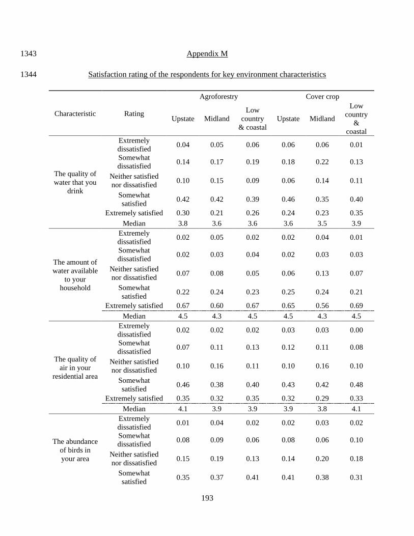
193
Appendix M 1343
Satisfaction rating of the respondents for key environment characteristics 1344
Characteristic Rating
Agroforestry Cover crop
Upstate Midland
Low
country
& coastal
Upstate Midland
Low
country
&
coastal
The quality of
water that you
drink
Extremely
dissatisfied 0.04 0.05 0.06 0.06 0.06 0.01
Somewhat
dissatisfied 0.14 0.17 0.19 0.18 0.22 0.13
Neither satisfied
nor dissatisfied 0.10 0.15 0.09 0.06 0.14 0.11
Somewhat
satisfied 0.42 0.42 0.39 0.46 0.35 0.40
Extremely satisfied 0.30 0.21 0.26 0.24 0.23 0.35
Median 3.8 3.6 3.6 3.6 3.5 3.9
The amount of
water available
to your
household
Extremely
dissatisfied 0.02 0.05 0.02 0.02 0.04 0.01
Somewhat
dissatisfied 0.02 0.03 0.04 0.02 0.03 0.03
Neither satisfied
nor dissatisfied 0.07 0.08 0.05 0.06 0.13 0.07
Somewhat
satisfied 0.22 0.24 0.23 0.25 0.24 0.21
Extremely satisfied 0.67 0.60 0.67 0.65 0.56 0.69
Median 4.5 4.3 4.5 4.5 4.3 4.5
The quality of
air in your
residential area
Extremely
dissatisfied 0.02 0.02 0.02 0.03 0.03 0.00
Somewhat
dissatisfied 0.07 0.11 0.13 0.12 0.11 0.08
Neither satisfied
nor dissatisfied 0.10 0.16 0.11 0.10 0.16 0.10
Somewhat
satisfied 0.46 0.38 0.40 0.43 0.42 0.48
Extremely satisfied 0.35 0.32 0.35 0.32 0.29 0.33
Median 4.1 3.9 3.9 3.9 3.8 4.1
The abundance
of birds in
your area
Extremely
dissatisfied 0.01 0.04 0.02 0.02 0.03 0.02
Somewhat
dissatisfied 0.08 0.09 0.06 0.08 0.06 0.10
Neither satisfied
nor dissatisfied 0.15 0.19 0.13 0.14 0.20 0.18
Somewhat
satisfied 0.35 0.37 0.41 0.41 0.38 0.31

194
Extremely satisfied 0.41 0.32 0.37 0.35 0.32 0.39
Median 4.1 3.8 4.0 4.0 3.9 3.9
The abundance
of deer in your
area
Extremely
dissatisfied 0.04 0.07 0.06 0.03 0.03 0.07
Somewhat
dissatisfied 0.10 0.10 0.17 0.14 0.09 0.10
Neither satisfied
nor dissatisfied 0.29 0.32 0.30 0.29 0.35 0.35
Somewhat
satisfied 0.31 0.27 0.25 0.30 0.26 0.19
Extremely satisfied 0.26 0.24 0.23 0.25 0.26 0.29
Median 3.6 3.5 3.4 3.6 3.6 3.5
The overall
state of the
environment in
your area
Extremely
dissatisfied 0.02 0.03 0.03 0.03 0.03 0.01
Somewhat
dissatisfied 0.12 0.16 0.13 0.15 0.15 0.17
Neither satisfied
nor dissatisfied 0.16 0.10 0.17 0.14 0.17 0.18
Somewhat
satisfied 0.46 0.49 0.46 0.48 0.46 0.42
Extremely satisfied 0.23 0.21 0.20 0.19 0.20 0.22
Median 3.8 3.7 3.7 3.7 3.6 3.7
1345
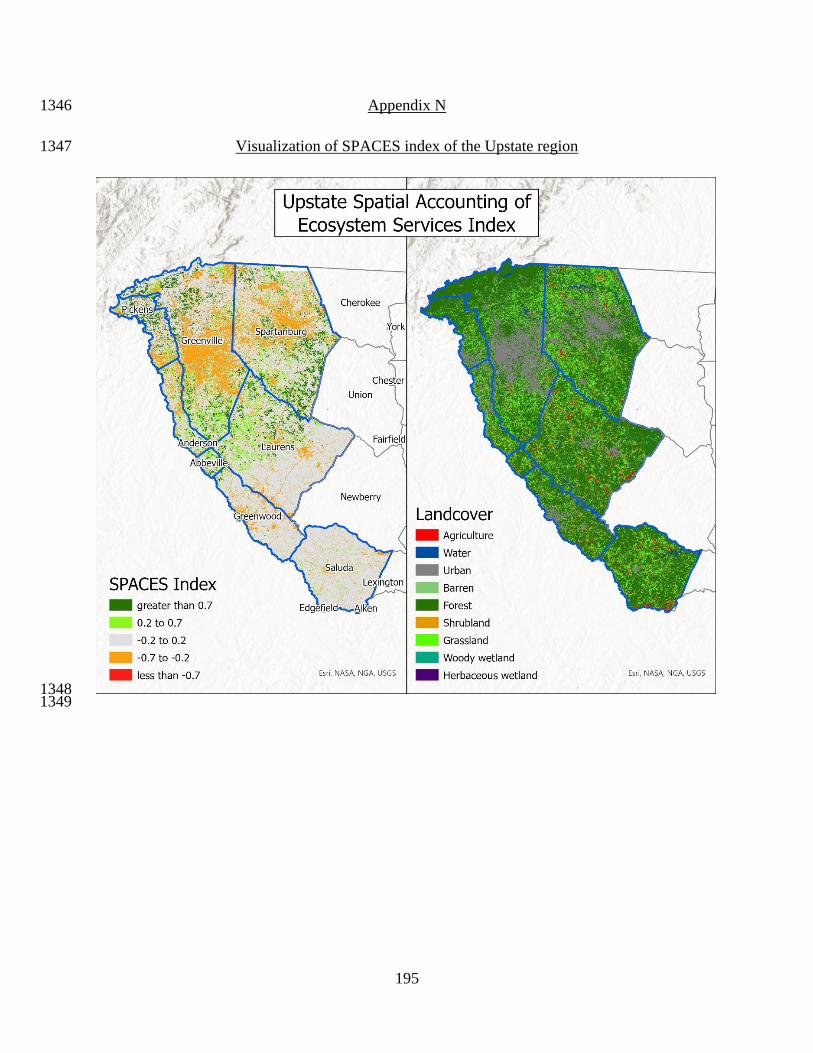
195
Appendix N 1346
Visualization of SPACES index of the Upstate region 1347
1348 1349
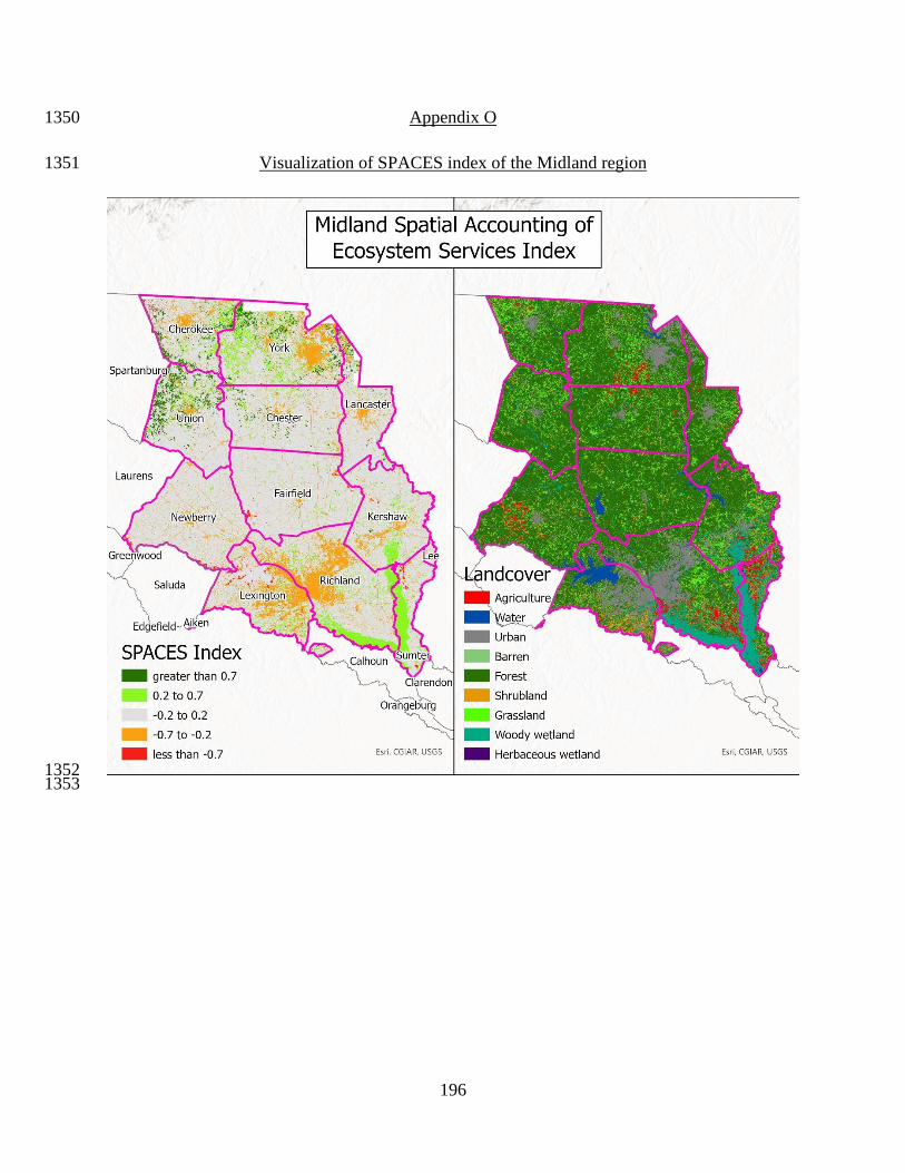
196
Appendix O 1350
Visualization of SPACES index of the Midland region 1351
1352 1353
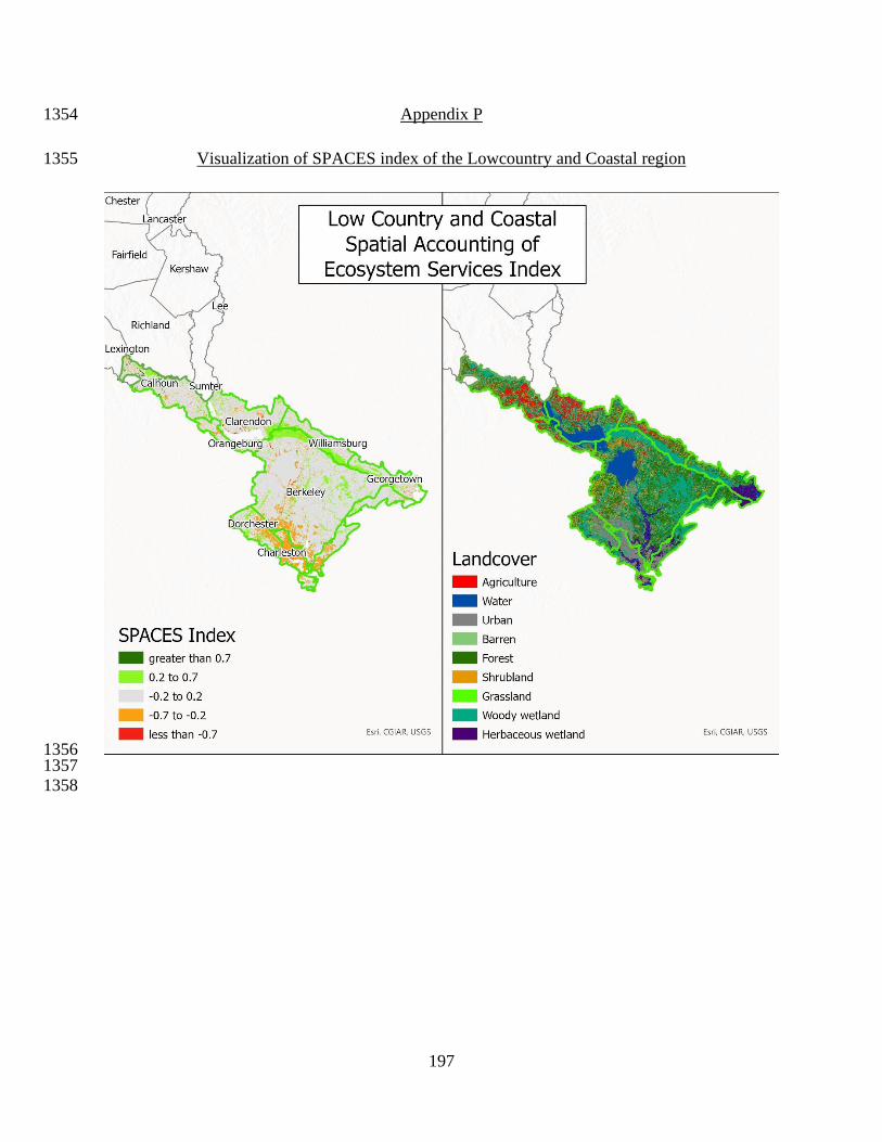
197
Appendix P 1354
Visualization of SPACES index of the Lowcountry and Coastal region 1355
1356 1357
1358

198
REFERENCES 1359
Abas, A. A., & Hashim, M. (2014). Change detection of runoff-urban growth relationship in 1360
urbanised watershed. In IOP Conference Series: Earth and Environmental Science (Vol. 1361
18). Institute of Physics Publishing. https://doi.org/10.1088/1755-1315/18/1/012040 1362
Abatzoglou, J. T. (2013). Development of gridded surface meteorological data for ecological 1363
applications and modelling. International Journal of Climatology, 33(1), 121–131. 1364
https://doi.org/10.1002/joc.3413 1365
Abdul-Wahab, S. A., & Abdo, J. (2010). The Effects of Demographic Factors on the 1366
Environmental Awareness of Omani Citizens. Human and Ecological Risk Assessment: An 1367
International Journal, 16(2), 380–401. https://doi.org/10.1080/10807031003670410 1368
Abram, N. K., Meijaard, E., Ancrenaz, M., Runting, R. K., Wells, J. A., Gaveau, D., … 1369
Mengersen, K. (2014). Spatially explicit perceptions of ecosystem services and land cover 1370
change in forested regions of Borneo. Ecosystem Services, 7, 116–127. 1371
https://doi.org/10.1016/j.ecoser.2013.11.004 1372
Aguilar, F. X., Obeng, E. A., & Cai, Z. (2018). Water quality improvements elicit consistent 1373
willingness-to-pay for the enhancement of forested watershed ecosystem services. 1374
Ecosystem Services, 30, 158–171. https://doi.org/10.1016/j.ecoser.2018.02.012 1375
Allen, R. G., Pereira, L. S., Raes, D., & Smith, M. (1998). FAO Irrigation and Drainage Paper 1376
No. 56: Crop Evapotranspiration. Rome, Italy: Food and Agriculture Organization (FAO) 1377
of the United Nation. Retrieved from https://www.researchgate.net/publication/235704197 1378
Arbuckle, J. G., & Roesch-McNally, G. (2015). Cover crop adoption in Iowa: The role of 1379
perceived practice characteristics. Journal of Soil and Water Conservation, 70(6), 418–429. 1380
https://doi.org/10.1016/j.forsciint.2012.03.015 1381
Arunkaumar, S., Bala, V. ., & Balaji, K. (2018). A study on attitude and behaviour of the 1382
respondents towards public examination with reference to erode. International Journal of 1383
Intellectual Advancements and Research in Engineering Computations, 6(2), 986–989. 1384
Retrieved from http://www.ijiarec.com/sites/default/files/articles/IJIAREC-18-295_986-1385
989.pdf 1386
Asah, S. T., Blahna, D. J., & Ryan, C. M. (2012). Involving Forest Communities in Identifying 1387
and Constructing Ecosystem Services: Millennium Assessment and Place Specificity. 1388
Journal of Forestry, 110(3), 149–156. https://doi.org/10.5849/jof.11-054 1389
Bagstad, K. J., Cohen, E., Ancona, Z. H., McNulty, S. G., & Sun, G. (2018). The sensitivity of 1390
ecosystem service models to choices of input data and spatial resolution. Applied 1391
Geography, 93, 25–36. https://doi.org/10.1016/J.APGEOG.2018.02.005 1392
Bagstad, K. J., Semmens, D. J., & Winthrop, R. (2013). Comparing approaches to spatially 1393
explicit ecosystem service modeling: A case study from the San Pedro River, Arizona. 1394
Ecosystem Services, 5, 40–50. https://doi.org/10.1016/j.ecoser.2013.07.007 1395
1396
199
Bai, Y., Ochuodho, T. O., & Yang, J. (2019). Impact of land use and climate change on water-1397
related ecosystem services in Kentucky, USA. Ecological Indicators, 102, 51–64. 1398
https://doi.org/10.1016/j.ecolind.2019.01.079 1399
Barbier, E. (1993). Sustainable use of wetlands. Valuing tropical wetland benefits: Economic 1400
methodologies and applications. The Geographical Journal, 159(1), 22–32. Retrieved from 1401
https://www.jstor.org/stable/pdf/3451486.pdf 1402
Barral, S. (2020). Conservation, finance, bureaucrats: managing time and space in the production 1403
of environmental intangibles. Journal of Cultural Economy, 1–15. 1404
https://doi.org/10.1080/17530350.2020.1846593 1405
Bateman, I. J., Carson, R. T., Day, B., Hanemann, W. M., Hanley, N., Hett, T., … Elgar, E. 1406
(2002). Economic Valuation With Stated Preference Techniques: A Manual. Retrieved from 1407
https://econweb.ucsd.edu/~rcarson/papers/BatemanBook.pdf 1408
Bateman, I. J., Harwood, A. R., Mace, G. M., Watson, R. T., Abson, D. J., Andrews, B., … 1409
Termansen, M. (2013). Bringing ecosystem services into economic decision-making: Land 1410
use in the United Kingdom. Science, 341(6141), 45–50. 1411
https://doi.org/10.1126/science.1234379 1412
Berkes, F., & Folke, C. (Eds.). (2000). Linking Social and Ecological Systems: Management 1413
Practices and Social Mechanisms for Building Resilience. New York: Cambridge 1414
University Press (CUP). 1415
Borselli, L., Cassi, P., & Torri, D. (2008). Prolegomena to sediment and flow connectivity in the 1416
landscape: A GIS and field numerical assessment. CATENA, 75(3), 268–277. 1417
https://doi.org/10.1016/J.CATENA.2008.07.006 1418
Bottorff, C. (2014). PAYMENTS FOR ECOSYSTEM SERVICES: Cases from the experience of 1419
U.S. communities. Charlottesville, Virginia. Retrieved from 1420
http://www.keylogeconomics.com/uploads/1/1/9/5/119575398/pes_casesfromuscommunitie1421
st_201407.pdf 1422
Bracken, L. J., Turnbull, L., Wainwright, J., & Bogaart, P. (2015). Sediment connectivity: a 1423
framework for understanding sediment transfer at multiple scales. Earth Surface Processes 1424
and Landforms, 40(2), 177–188. https://doi.org/10.1002/esp.3635 1425
Branton, M. A., & Richardson, J. S. (2014). A test of the umbrella species approach in restored 1426
floodplain ponds. Journal of Applied Ecology, 51(3), 776–785. 1427
https://doi.org/10.1111/1365-2664.12248 1428
Brent, D. A., Gangadharan, L., Lassiter, A., Leroux, A., & Raschky, P. A. (2017). Valuing 1429
environmental services provided by local stormwater management. Water Resources 1430
Research, 53(6), 4907–4921. https://doi.org/10.1002/2016WR019776 1431
Brown, M. G., & Quinn, J. E. (2018). Zoning does not improve the availability of ecosystem 1432
services in urban watersheds. A case study from Upstate South Carolina, USA. Ecosystem 1433
Services, 34, 254–265. https://doi.org/10.1016/J.ECOSER.2018.04.009 1434
1435

200
Brox, J. A., Kumar, R. C., & Stollery, K. R. (1996). WILLINGNESS TO PAY FOR WATER 1436
QUALITY AND SUPPLY ENHANCEMENTS IN THE GRAND RIVER WATERSHED. 1437
Canadian Water Resources Journal, 21(3), 275–288. https://doi.org/10.4296/cwrj2103275 1438
Brundtland, G. (1987). Report of the World Commission on Environment and Development: Our 1439
Common Future Towards Sustainable Development. 1440
Bugalho, M. N., Dias, F. S., Briñas, B., & Cerdeira, J. O. (2016). Using the high conservation 1441
value forest concept and Pareto optimization to identify areas maximizing biodiversity and 1442
ecosystem services in cork oak landscapes. Agroforestry Systems, 90(1), 35–44. 1443
https://doi.org/10.1007/s10457-015-9814-x 1444
BUREAU OF WATER, S. D. (2008). WATER CLASSIFICATIONS and STANDARDS. 1445
Columbia, SC. 1446
BUREAU OF WATER, S. D. (2011). Stormwater Permit Notice of Intent (NOI) Water Quality 1447
Information Tool Web Application Supporting Documentation. Retrieved from 1448
www.scdhec.gov/stormwater 1449
Butler, B. J., & Wear, D. N. (2013). The Southern Forest Futures Project Technical Report: 1450
Chapter 6 Forest Ownership Dynamics of Southern Forests. Retrieved from 1451
https://www.srs.fs.usda.gov/futures/technical-report/06.html 1452
Calderon, M. M., Anit, K. P. A., Palao, L. K. M., & Lasco, R. D. (2012). Households’ 1453
Willingness to Pay for Improved Watershed Services of the Layawan Watershed in 1454
Oroquieta City, Philippines. Journal of Sustainable Development, 6(1), p1. 1455
https://doi.org/10.5539/jsd.v6n1p1 1456
Camara, M., Jamil, N. R., & Abdullah, A. F. Bin. (2019, December 1). Impact of land uses on 1457
water quality in Malaysia: a review. Ecological Processes. Springer Verlag. 1458
https://doi.org/10.1186/s13717-019-0164-x 1459
Campbell, E. T., & Tilley, D. R. (2014). Valuing ecosystem services from Maryland forests 1460
using environmental accounting. Ecosystem Services, 7, 141–151. 1461
https://doi.org/10.1016/j.ecoser.2013.10.003 1462
Canqiang, Z., Wenhua, L., Biao, Z., & Moucheng, L. (2012). Water Yield of Xitiaoxi River 1463
Basin Based on InVEST Modeling. Journal of Resources and Ecology, 3(1), 50–54. 1464
https://doi.org/10.5814/j.issn.1674-764x.2012.01.008 1465
Carpenter, S. R., Stanley, E. H., & Vander Zanden, M. J. (2011). State of the world’s freshwater 1466
ecosystems: Physical, chemical, and biological changes. Annual Review of Environment and 1467
Resources, 36, 75–99. https://doi.org/10.1146/annurev-environ-021810-094524 1468
Castro, A. J., Vaughn, C. C., García-Llorente, M., Julian, J. P., & Atkinson, C. L. (2016). 1469
Willingness to Pay for Ecosystem Services among Stakeholder Groups in a South-Central 1470
U.S. Watershed with Regional Conflict. Journal of Water Resources Planning and 1471
Management, 142(9), 05016006. https://doi.org/10.1061/(ASCE)WR.1943-5452.0000671 1472
Champ, P., Boyle, K., & Brown, T. (2003). A Primer on Nonmarket Valuation. (Patricia A. 1473
Champ, K. J. Boyle, & T. C. Brown, Eds.) (Vol. 3). Dordrecht: Springer Netherlands. 1474
https://doi.org/10.1007/978-94-007-0826-6 1475

201
Champ, Patrica A., Boyle, K. J., & Brown, T. C. (2017). The Economics of Non-Market Goods 1476
and Resources: A Primer on Nonmarket Valuation. (I. J. Bateman, Ed.). 1477
Champ, Patricia A, Moore, R., & Bishop, R. C. (2009). A Comparison of Approaches to Mitigate 1478
Hypothetical Bias. Agricultural and Resource Economics Review (Vol. 38). 1479
Chan, K. M. A., Shaw, M. R., Cameron, D. R., Underwood, E. C., & Daily, G. C. (2006). 1480
Conservation Planning for Ecosystem Services. PLoS Biology, 4(11), e379. 1481
https://doi.org/10.1371/journal.pbio.0040379 1482
Chen, J., Theller, L., Gitau, M. W., Engel, B. A., & Harbor, J. M. (2017). Urbanization impacts 1483
on surface runoff of the contiguous United States. Journal of Environmental Management, 1484
187, 470–481. https://doi.org/10.1016/j.jenvman.2016.11.017 1485
Chen, X., Viña, A., Shortridge, A., An, L., Liu, J. 2014, Chen, X., … Liu, J. (2014). Assessing 1486
the Effectiveness of Payments for Ecosystem Services: an Agent-Based Modeling 1487
Approach. https://doi.org/10.5751/ES-05578-190107 1488
Chiavacci, S. J., & Pindilli, E. J. (2020). Trends in biodiversity and habitat quantification tools 1489
used for market‐based conservation in the United States. Conservation Biology, 34(1), 125–1490
136. https://doi.org/10.1111/cobi.13349 1491
Choi, D. S., Ready, R. C., & Shortle, J. S. (2020). Valuing water quality benefits from adopting 1492
best management practices: A spatial approach. Journal of Environmental Quality, 49(3), 1493
582–592. https://doi.org/10.1002/jeq2.20005 1494
Clay, L., Motallebi, M., & Song, B. (2019). An Analysis of Common Forest Management 1495
Practices for Carbon Sequestration in South Carolina. Forests, 10(11), 949. 1496
https://doi.org/10.3390/f10110949 1497
Clay, L., Perkins, K., Motallebi, M., Plastina, A., & Farmaha, B. S. (2020). The Perceived 1498
Benefits, Challenges, and Environmental Effects of Cover Crop Implementation in South 1499
Carolina. Agriculture, 10(9), 372. https://doi.org/10.3390/agriculture10090372 1500
Cooper, K. (2011). Evaluation of the Relationship Between the RUSLE R-Factor and Mean 1501
Annual Precipitation. Retrieved from 1502
https://www.engr.colostate.edu/~pierre/ce_old/Projects/linkfiles/Cooper R-factor-Final.pdf 1503
Cosgrove, W. J., & Loucks, D. P. (2015). Water management: Current and future challenges and 1504
research directions. Water Resources Research, 51(6), 4823–4839. 1505
https://doi.org/10.1002/2014WR016869 1506
Costanza, R., d’Arge, R., de Groot, R., Farber, S., Grasso, M., Hannon, B., … van den Belt, M. 1507
(1997). The value of the world’s ecosystem services and natural capital. Nature, 387(6630), 1508
253–260. https://doi.org/10.1038/387253a0 1509
Cranford, M., & Mourato, S. (2014). Credit-Based Payments for Ecosystem Services: Evidence 1510
from a Choice Experiment in Ecuador. World Development, 64. 1511
https://doi.org/10.1016/j.worlddev.2014.06.019 1512
1513
202
Cumming, G. S. (2011). Spatial resilience: Integrating landscape ecology, resilience, and 1514
sustainability. Landscape Ecology, 26(7), 899–909. https://doi.org/10.1007/s10980-011-1515
9623-1 1516
Cummings, R. G., & Taylor, L. O. (1999). Unbiased value estimates for environmental goods: A 1517
cheap talk design for the contingent valuation method. American Economic Review. 1518
American Economic Association. https://doi.org/10.1257/aer.89.3.649 1519
Daily, G. C., Polasky, S., Goldstein, J., Kareiva, P. M., Mooney, H. A., Pejchar, L., … 1520
Shallenberger, R. (2009). Ecosystem services in decision making: time to deliver. Frontiers 1521
in Ecology and the Environment, 7(1), 21–28. https://doi.org/10.1890/080025 1522
Daniel McFadden. (1973). Conditional Logit Analysis of Qualitative Choice Behavior. Frontiers 1523
in Econometrics, 105–142. Retrieved from 1524
https://eml.berkeley.edu/reprints/mcfadden/zarembka.pdf 1525
de Groot, R. S., Alkemade, R., Braat, L., Hein, L., & Willemen, L. (2010). Challenges in 1526
integrating the concept of ecosystem services and values in landscape planning, 1527
management and decision making. Ecological Complexity, 7(3), 260–272. 1528
https://doi.org/10.1016/j.ecocom.2009.10.006 1529
de Pedro, L., Perera-Fernández, L. G., López-Gallego, E., Pérez-Marcos, M., & Sanchez, J. A. 1530
(2020). The Effect of Cover Crops on the Biodiversity and Abundance of Ground-Dwelling 1531
Arthropods in a Mediterranean Pear Orchard. Agronomy, 10(4), 580. 1532
https://doi.org/10.3390/agronomy10040580 1533
Dennedy-Frank, P. J., Muenich, R. L., Chaubey, I., & Ziv, G. (2016). Comparing two tools for 1534
ecosystem service assessments regarding water resources decisions. Journal of 1535
Environmental Management, 177, 331–340. https://doi.org/10.1016/j.jenvman.2016.03.012 1536
Dhanavandan, S. (2016). APPLICATION OF GARRET RANKING TECHNIQUE: 1537
PRACTICAL APPROACH. International Journal of Library and Information Studies, 6(3). 1538
Retrieved from www.ijlis.org 1539
Díaz, S., Demissew, S., Carabias, J., Joly, C., Lonsdale, M., Ash, N., … Zlatanova, D. (2015, 1540
June 1). The IPBES Conceptual Framework - connecting nature and people. Current 1541
Opinion in Environmental Sustainability. Elsevier. 1542
https://doi.org/10.1016/j.cosust.2014.11.002 1543
Doherty, E., Murphy, G., Hynes, S., & Buckley, C. (2014). Valuing ecosystem services across 1544
water bodies: Results from a discrete choice experiment. Ecosystem Services, 7, 89–97. 1545
https://doi.org/10.1016/j.ecoser.2013.09.003 1546
Donohue, R. J., Roderick, M. L., & McVicar, T. R. (2012). Roots, storms and soil pores: 1547
Incorporating key ecohydrological processes into Budyko’s hydrological model. Journal of 1548
Hydrology, 436–437, 35–50. https://doi.org/10.1016/j.jhydrol.2012.02.033 1549
Dunn, M., Ulrich-Schad, J. D., Prokopy, L. S., Myers, R. L., Watts, C. R., & Scanlon, K. (2016). 1550
Perceptions and use of cover crops among early adopters: Findings from a national survey. 1551
Journal of Soil and Water Conservation, 71(1), 29–40. https://doi.org/10.2489/jswc.71.1.29 1552
1553
203
Ecoagriculture Partners. (2011, October). Payments for watershed services in the United States 1554
Cost-effective strategies to align landowner incentives for abundant clean water. 1555
Ecoagriculture Policy Focus. 1556
Edwards, C. A. (1990). Sustainable Agricultural Systems (1st ed.). (C. A. Edwards, R. Lal, P. 1557
Madden, R. H. Miller, & G. House, Eds.) (1st ed.). CRC Press. 1558
https://doi.org/10.1201/9781003070474 1559
Elhakeem, A., van der Werf, W., Ajal, J., Lucà, D., Claus, S., Vico, R. A., & Bastiaans, L. 1560
(2019). Cover crop mixtures result in a positive net biodiversity effect irrespective of 1561
seeding configuration. Agriculture, Ecosystems and Environment, 285, 106627. 1562
https://doi.org/10.1016/j.agee.2019.106627 1563
Elwell, T. L., Gelcich, S., Gaines, S. D., & López-Carr, D. (2018). Using people’s perceptions of 1564
ecosystem services to guide modeling and management efforts. Science of The Total 1565
Environment, 637–638, 1014–1025. https://doi.org/10.1016/J.SCITOTENV.2018.04.052 1566
Engel, S., Pagiola, S., & Wunder, S. (2008). Designing payments for environmental services in 1567
theory and practice: An overview of the issues. Ecological Economics. 1568
https://doi.org/10.1016/j.ecolecon.2008.03.011 1569
Ernst, K. M., & van Riemsdijk, M. (2013). Climate change scenario planning in Alaska’s 1570
National Parks: Stakeholder involvement in the decision-making process. Applied 1571
Geography, 45, 22–28. https://doi.org/10.1016/j.apgeog.2013.08.004 1572
ESRI. (2017). USA Soils Erodibility Factor | ArcGIS Hub. Retrieved August 19, 2020, from 1573
https://www.arcgis.com/home/item.html?id=ac1bc7c30bd4455e85f01fc51055e586#:~:text=1574
Soil erodibility factor%2C also known,detachment and movement by water. 1575
Fageria, N. K. (2012). Role of Soil Organic Matter in Maintaining Sustainability of Cropping 1576
Systems. Communications in Soil Science and Plant Analysis, 43(16), 2063–2113. 1577
https://doi.org/10.1080/00103624.2012.697234 1578
Fauzi, A., & Anna, Z. (2013). The complexity of the institution of payment for environmental 1579
services: A case study of two Indonesian PES schemes. Ecosystem Services, 6, 54–63. 1580
https://doi.org/10.1016/J.ECOSER.2013.07.003 1581
Fischer, C., Damm, C., Foeckler, F., Gelhaus, M., Gerstner, L., Harris, R. M. B., … Scholz, M. 1582
(2019). The “Habitat Provision” Index for Assessing Floodplain Biodiversity and 1583
Restoration Potential as an Ecosystem Service—Method and Application. Frontiers in 1584
Ecology and Evolution, 7, 483. https://doi.org/10.3389/fevo.2019.00483 1585
Foley, J. A. (2005). Global Consequences of Land Use. Science, 309(5734), 570–574. 1586
https://doi.org/10.1126/science.1111772 1587
Ford, J. B. (2017). Amazon’s Mechanical Turk: A Comment. Journal of Advertising, 46(1), 156–1588
158. https://doi.org/10.1080/00913367.2016.1277380 1589
Forest Trends, The Katoomba Group, & UN Environment Programme (UNEP). (2008). 1590
Payments for ecosystem services: Getting Started. Retrieved from 1591
https://wedocs.unep.org/handle/20.500.11822/9150 1592
204
Fu, B. P. (1981). On the calculation of the evaporation from land surface. Chinese Journal of 1593
Atmospheric Sciences, 5, 23–31. Retrieved from 1594
http://en.cnki.com.cn/Article_en/CJFDTOTAL-DQXK198101002.htm 1595
Gabriel, J. L., Garrido, A., & Quemada, M. (2013). Cover crops effect on farm benefits and 1596
nitrate leaching: Linking economic and environmental analysis. Agricultural Systems, 121, 1597
23–32. https://doi.org/10.1016/J.AGSY.2013.06.004 1598
Gao, J., Li, F., Gao, H., Zhou, C., & Zhang, X. (2017). The impact of land-use change on water-1599
related ecosystem services: a study of the Guishui River Basin, Beijing, China. Journal of 1600
Cleaner Production, 163, S148–S155. https://doi.org/10.1016/j.jclepro.2016.01.049 1601
Ge, J., Kling, C., & Herriges, J. (2013). How Much is Clean Water Worth? Valuing Water 1602
Quality Improvement Using A Meta Analysis. 1603
Goldman, R. L., Thompson, B. H., & Daily, G. C. (2007). Institutional incentives for managing 1604
the landscape: Inducing cooperation for the production of ecosystem services. Ecological 1605
Economics, 64(2), 333–343. https://doi.org/10.1016/j.ecolecon.2007.01.012 1606
Greene, W. H. (1980). Maximum likelihood estimation of econometric frontier functions. 1607
Journal of Econometrics, 13(1), 27–56. https://doi.org/10.1016/0304-4076(80)90041-X 1608
Greiber, T. (2009). Payments for Ecosystem Services. Legal and Institutional Frameworks. (T. 1609
Greiber, Ed.). Gland, Switzerland: IUCN. Retrieved from www.iucn.org/law 1610
Grima, N., Singh, S. J., Smetschka, B., & Ringhofer, L. (2016). Payment for Ecosystem Services 1611
(PES) in Latin America: Analysing the performance of 40 case studies. Ecosystem Services, 1612
17, 24–32. https://doi.org/10.1016/j.ecoser.2015.11.010 1613
Hamel, P., & Guswa, A. J. (2015). Uncertainty analysis of a spatially explicit annual water-1614
balance model: case study of the Cape Fear basin, North Carolina. Hydrology and Earth 1615
System Sciences, 19(2), 839–853. https://doi.org/10.5194/hess-19-839-2015 1616
Hanson, J. D., Hendrickson, J., & Archer, D. (2008). Challenges for maintaining sustainable 1617
agricultural systems in the United States. Renewable Agriculture and Food Systems, 23(4), 1618
325–334. https://doi.org/10.1017/S1742170507001974 1619
Harder, S. V., Gellici, J. A., Wachob, A., & Pellett, C. A. (2020). Overview of the South 1620
Carolina State and River Basin Planning Framework. The Journal of South Carolina Water 1621
Resources, (6), 56–61. https://doi.org/10.34068/jscwr.06.06 1622
Hargrove, W. L., & Heyman, J. M. (2020). A Comprehensive Process for Stakeholder 1623
Identification and Engagement in Addressing Wicked Water Resources Problems. Land, 1624
9(4), 119. https://doi.org/10.3390/land9040119 1625
Hauber, A. B., González, J. M., Groothuis-Oudshoorn, C. G. M., Prior, T., Marshall, D. A., 1626
Cunningham, C., … Bridges, J. F. P. (2016). Statistical methods for the analysis of discrete 1627
choice experiments: A report of the ISPOR Conjoint Analysis Good Research Practices 1628
Task Force. Value in Health, 19(4), 300–315. https://doi.org/10.1016/j.jval.2016.04.004 1629
1630
205
Hein, L., Bagstad, K., Edens, B., Obst, C., De Jong, R., & Lesschen, J. P. (2016). Defining 1631
ecosystem assets for natural capital accounting. PLoS ONE, 11(11). 1632
https://doi.org/10.1371/journal.pone.0164460 1633
Hein, L., van Koppen, K., de Groot, R. S., & van Ierland, E. C. (2006). Spatial scales, 1634
stakeholders and the valuation of ecosystem services. Ecological Economics, 57(2), 209–1635
228. https://doi.org/10.1016/j.ecolecon.2005.04.005 1636
Hobbs, P. R. (2007). Conservation Agriculture: What is it and why is it important for future 1637
sustainable food production. Journal of Agriculture Science, 145(2), 127–137. 1638
https://doi.org/10.1017/S0021859607006892 1639
Hole, A. R. (2007). Fitting Mixed Logit Models by Using Maximum Simulated Likelihood. The 1640
Stata Journal: Promoting Communications on Statistics and Stata, 7(3), 388–401. 1641
https://doi.org/10.1177/1536867X0700700306 1642
Hole, A. R. (2013). Mixed logit modelling in Stata: An overview. In UK Stata Users Group 1643
Meeting (pp. 1–43). 1644
Holmes, T. P., & Adamowicz, W. L. (2003). Attribute-Based Methods. In Patricia A. Champ, K. 1645
J. Boyle, & T. C. Brown (Eds.), A Primer on Nonmarket Valuation. The Economics of Non-1646
Market Goods and Resources (pp. 171–219). https://doi.org/10.1007/978-94-007-0826-6_6 1647
Hoorman, J. J., Islam, R., Sundermeier, A., & Reeder, R. (2009). Using Cover Crops to Convert 1648
to No-Till. Crops and Soils, 42(6). 1649
Hoyer, R., & Chang, H. (2014). Assessment of freshwater ecosystem services in the tualatin and 1650
Yamhill basins under climate change and urbanization. Applied Geography, 53, 402–416. 1651
https://doi.org/10.1016/j.apgeog.2014.06.023 1652
Huang, J., Zhan, J., Yan, H., Wu, F., & Deng, X. (2013). Evaluation of the impacts of land use 1653
on water quality: A case study in the Chaohu lake basin. The Scientific World Journal, 1654
2013. https://doi.org/10.1155/2013/329187 1655
Hughes, W. B., Abrahamsen, T. A., Maluk, T. L., Reuber, E. J., & Wilhelm, L. J. (2000). Water 1656
Quality in the Santee River Basin and Coastal Drainages, North and South Carolina, 1995–1657
98: U.S. Geological Survey Circular 1206. Retrieved from 1658
https://pubs.usgs.gov/circ/circ1206/introduction.htm 1659
Hung, C. L. J., James, L. A., & Carbone, G. J. (2018). Impacts of urbanization on stormflow 1660
magnitudes in small catchments in the Sandhills of South Carolina, USA. Anthropocene, 23, 1661
17–28. https://doi.org/10.1016/j.ancene.2018.08.001 1662
Ingram, J. C., Wilkie, D., Clements, T., McNab, R. B., Nelson, F., Baur, E. H., … Foley, C. A. 1663
H. (2014). Evidence of Payments for Ecosystem Services as a mechanism for supporting 1664
biodiversity conservation and rural livelihoods. Ecosystem Services, 7. 1665
https://doi.org/10.1016/j.ecoser.2013.12.003 1666
Jack, B. K., Kousky, C., & Sims, K. R. E. (2008). Designing payments for ecosystem services: 1667
Lessons from previous experience with incentive-based mechanisms. Proceedings of the 1668
National Academy of Sciences. https://doi.org/10.1073/pnas.0705503104 1669
206
Kaspar, T. C., & Singer, J. W. (2011). The Use of Cover Crops to Manage Soil. USDA-ARS, 1670
321–337. https://doi.org/10.2136/2011.soilmanagement.c21 1671
Kaushal, S. S., Gold, A. J., & Mayer, P. M. (2017, October 24). Land use, climate, and water 1672
resources-global stages of interaction. Water (Switzerland). MDPI AG. 1673
https://doi.org/10.3390/w9100815 1674
Keller, A. A., Fournier, E., & Fox, J. (2015). Minimizing impacts of land use change on 1675
ecosystem services using multi-criteria heuristic analysis. Journal of Environmental 1676
Management. https://doi.org/10.1016/j.jenvman.2015.03.017 1677
Khan, I., Lei, H., Ali, G., Ali, S., & Zhao, M. (2019). Public attitudes, preferences and 1678
willingness to pay for river ecosystem services. International Journal of Environmental 1679
Research and Public Health, 16(19). https://doi.org/10.3390/ijerph16193707 1680
Khan, I., & Zhao, M. (2019). Water resource management and public preferences for water 1681
ecosystem services: A choice experiment approach for inland river basin management. 1682
Science of the Total Environment, 646, 821–831. 1683
https://doi.org/10.1016/j.scitotenv.2018.07.339 1684
Kindu, M., Schneider, T., Teketay, D., & Knoke, T. (2016). Changes of ecosystem service values 1685
in response to land use/land cover dynamics in Munessa-Shashemene landscape of the 1686
Ethiopian highlands. Science of the Total Environment, 547, 137–147. 1687
https://doi.org/10.1016/j.scitotenv.2015.12.127 1688
Kosoy, N., & Corbera, E. (2010). Payments for ecosystem services as commodity fetishism. 1689
Ecological Economics, 69(6), 1228–1236. https://doi.org/10.1016/j.ecolecon.2009.11.002 1690
Kreuter, U. P., Harris, H. G., Matlock, M. D., & Lacey, R. E. (2001). Change in ecosystem 1691
service values in the san antonio area, Texas. Ecological Economics, 39(3), 333–346. 1692
https://doi.org/10.1016/S0921-8009(01)00250-6 1693
Krkoška lorencová, E., Harmáčková, Z. V., Landová, L., Pártl, A., & Vačkář, D. (2016). 1694
Assessing impact of land use and climate change on regulating ecosystem services in the 1695
czech republic. Ecosystem Health and Sustainability, 2(3), e01210. 1696
https://doi.org/10.1002/ehs2.1210 1697
Kuhfeld, W. (2000). Multinomial Logit, Discrete Choice Modeling. Auckland. Retrieved from 1698
https://www.stat.auckland.ac.nz/~reilly/Choice.pdf 1699
Lackstrom, K., Glick, P., Dow, K., Stein, B. A., Peterson, M. N., Chin, E., & Clark, K. (2018). 1700
Climate Change and Conservation in the Southeast: A Review of State Wildlife Action 1701
Plans. Retrieved from http://go.ncsu.edu/se_swap_review_report. 1702
Lancaster, K. J. (1966). A New Approach to Consumer Theory. Source: Journal of Political 1703
Economy (Vol. 74). 1704
Land Trust Alliance. (n.d.). Find A Land Trust | Land Trust Alliance. Retrieved December 4, 1705
2020, from https://www.findalandtrust.org/states/south carolina45/land_trusts 1706
1707
207
Lang, Y., Song, W., & Zhang, Y. (2017). Responses of the water-yield ecosystem service to 1708
climate and land use change in Sancha River Basin, China. Physics and Chemistry of the 1709
Earth, Parts A/B/C, 101, 102–111. https://doi.org/10.1016/j.pce.2017.06.003 1710
Lautenbach, S., Kugel, C., Lausch, A., & Seppelt, R. (2011). Analysis of historic changes in 1711
regional ecosystem service provisioning using land use data. Ecological Indicators, 11(2), 1712
676–687. https://doi.org/10.1016/j.ecolind.2010.09.007 1713
Lawler, J. J., Lewis, D. J., Nelson, E., Plantinga, A. J., Polasky, S., Withey, J. C., … Radeloff, V. 1714
C. (2014). Projected land-use change impacts on ecosystem services in the United States. 1715
Proceedings of the National Academy of Sciences of the United States of America, 111(20), 1716
7492–7497. https://doi.org/10.1073/pnas.1405557111 1717
Leviston, Z., Walker, I., Green, M., & Price, J. (2018). Linkages between ecosystem services and 1718
human wellbeing: A Nexus Webs approach. Ecological Indicators, 93, 658–668. 1719
https://doi.org/10.1016/j.ecolind.2018.05.052 1720
Li, S., Yang, H., Lacayo, M., Liu, J., & Lei, G. (2018). Impacts of Land-Use and Land-Cover 1721
Changes on Water Yield: A Case Study in Jing-Jin-Ji, China. Sustainability, 10(4), 960. 1722
https://doi.org/10.3390/su10040960 1723
Lin, Y.-P., Chen, C.-J., Lien, W.-Y., Chang, W.-H., Petway, J., & Chiang, L.-C. (2019). 1724
Landscape Conservation Planning to Sustain Ecosystem Services under Climate Change. 1725
Sustainability, 11(5), 1393. https://doi.org/10.3390/su11051393 1726
Liu, S., Costanza, R., Farber, S., & Troy, A. (2010). Valuing ecosystem services Theory, 1727
practice, and the need for a transdisciplinary synthesis. Ann. N.Y. Acad. Sci, 1185, 54–78. 1728
Retrieved from https://www.pdx.edu/sites/www.pdx.edu.sustainability/files/Liu et al. 2010 - 1729
Valuing Ecosystem Services.pdf 1730
Liu, S., Costanza, R., Troy, A., D’Aagostino, J., & Mates, W. (2010). Valuing New Jersey’s 1731
ecosystem services and natural capital: A spatially explicit benefit transfer approach. 1732
Environmental Management, 45(6), 1271–1285. https://doi.org/10.1007/s00267-010-9483-5 1733
Liu, Y., Li, J., & Zhang, H. (2012). An ecosystem service valuation of land use change in 1734
Taiyuan City, China. Ecological Modelling, 225, 127–132. 1735
https://doi.org/10.1016/j.ecolmodel.2011.11.017 1736
Louviere, J. J. (2001). Choice experiments: An overview of concepts and issues. In J. Bennett & 1737
R. Blamey (Eds.), The choice modelling approach to environmental valuation. 1738
Northampton, Massachusetts: Edward Elgar Publishing Inc. 1739
Mangiafico, S. S., Obropta, C. C., & Rossi-Griffin, E. (2012). Demographic Factors Influence 1740
Environmental Values: A Lawn-Care Survey of Homeowners in New Jersey. Journal of 1741
Extension, 50(1). Retrieved from www.joe.org/joe/2012february/rb6p.shtml 1742
Manski, C. F. (1977). The structure of random utility models. Theory and Decision, 8(3), 229–1743
254. https://doi.org/10.1007/BF00133443 1744
1745
208
Marsh, D. K. (2014). Valuation of water quality improvements in the Karapiro catchment: A 1746
choice modelling approach Consumer switching in retail electricity markets View project 1747
Natural Capital and Environmental Decision Making View project. Retrieved from 1748
https://www.researchgate.net/publication/228389071 1749
Mase, A. S., Gramig, B. M., & Prokopy, L. S. (2017). Climate change beliefs, risk perceptions, 1750
and adaptation behavior among Midwestern U.S. crop farmers. Climate Risk Management, 1751
15, 8–17. https://doi.org/10.1016/J.CRM.2016.11.004 1752
McCarney-Castle, K., Childress, T. M., & Heaton, C. R. (2017). Sediment source identification 1753
and load prediction in a mixed-use Piedmont watershed, South Carolina. Journal of 1754
Environmental Management, 185, 60–69. https://doi.org/10.1016/j.jenvman.2016.10.036 1755
McNeely, J. A. (1990). The future of national parks. Environment, 32(1), 16–41. 1756
https://doi.org/10.1080/00139157.1990.9928997 1757
Mercer, D. E., Cooley, D., & Hamilton, K. (2011). Taking Stock: Payments for Forest Ecosystem 1758
Services in the United States. Retrieved from 1759
https://www.fs.usda.gov/treesearch/pubs/38987 1760
Millenium Ecosystem Assessment. (2005). Ecosystems and Human Well-Being: Synthesis. 1761
Washington, DC. Retrieved from www.islandpress.org 1762
Miller, J. R., & Hobbs, R. J. (2002, April 1). Conservation where people live and work. 1763
Conservation Biology. John Wiley & Sons, Ltd. https://doi.org/10.1046/j.1523-1764
1739.2002.00420.x 1765
Motallebi, M., Hoag, D. L., Tasdighi, A., Arabi, M., & Osmond, D. L. (2017). An economic 1766
inquisition of water quality trading programs, with a case study of Jordan Lake, NC. 1767
Journal of Environmental Management. https://doi.org/10.1016/j.jenvman.2017.02.039 1768
Motoshita, M., Ono, Y., Finkbeiner, M., & Inaba, A. (2016). The Effect of Land Use on 1769
Availability of Japanese Freshwater Resources and Its Significance for Water Footprinting. 1770
Sustainability, 8(1), 86. https://doi.org/10.3390/su8010086 1771
Moultrie News. (2019, November 15). Return of nesting birds to Crab Bank Seabird Sanctuary 1772
one step closer. Retrieved from https://www.moultrienews.com/community-news/return-of-1773
nesting-birds-to-crab-bank-seabird-sanctuary-one/article_0c35ba10-0706-11ea-95c3-1774
1b4f9e8e5466.html 1775
Muhammad Nauman Sadiq, B., Muhammad Ishaq, H., Nauman Sadiq α, M., & Muhammad 1776
Ishaq σ, H. (2014). The Effect of Demographic Factors on the Behavior of Investors during 1777
the Choice of Investment: Evidence from Twin Cities of Pakistan. Type: Double Blind Peer 1778
Reviewed International Research Journal Publisher: Global Journals Inc, 14. 1779
Mulder, J., & de Bruijne, M. (2019). Willingness of Online Respondents to Participate in 1780
Alternative Modes of Data Collection. Survey Practice, 12(1), 1–11. 1781
https://doi.org/10.29115/sp-2019-0001 1782
Murphy, J. J., Stevens, T. H., & Weatherhead, D. (2005). Is cheap talk effective at eliminating 1783
hypothetical bias in a provision point mechanism? Environmental and Resource Economics, 1784
30(3), 327–343. https://doi.org/10.1007/s10640-004-4224-y 1785

209
Murty, P. L. N., Sandhya, K. G., Bhaskaran, P. K., Jose, F., Gayathri, R., Balakrishnan Nair, T. 1786
M., … Shenoi, S. S. C. (2014). A coupled hydrodynamic modeling system for PHAILIN 1787
cyclone in the Bay of Bengal. Coastal Engineering, 93, 71–81. 1788
https://doi.org/10.1016/J.COASTALENG.2014.08.006 1789
National Weather Service. (n.d.). Advanced Hydrologic Prediction Service. Retrieved September 1790
2, 2020, from https://water.weather.gov/precip/download.php 1791
Nelson, E., Ennaanay, D., Wolny, S., Olwero, N., Vigerstol, K., Penning-ton, D., … Douglass, J. 1792
(2018). InVEST 3.6.0 User’s Guide. Retrieved from 1793
http://data.naturalcapitalproject.org/nightly-build/invest-users-1794
guide/InVEST_3.6.0_Documentation.pdf 1795
Noe, R. R., Keeler, B. L., Kilgore, M. A., Taff, S. J., & Polasky, S. (2017). Mainstreaming 1796
ecosystem services in state-level conservation planning: Progress and future needs. Ecology 1797
and Society, 22(4). https://doi.org/10.5751/ES-09581-220404 1798
Norgaard, R. B. (2010). Ecosystem services: From eye-opening metaphor to complexity blinder. 1799
Ecological Economics, 69(6), 1219–1227. https://doi.org/10.1016/j.ecolecon.2009.11.009 1800
Olander, L. P., Johnston, R. J., Tallis, H., Kagan, J., Maguire, L. A., Polasky, S., … Palmer, M. 1801
(2018). Benefit relevant indicators: Ecosystem services measures that link ecological and 1802
social outcomes. Ecological Indicators, 85, 1262–1272. 1803
https://doi.org/10.1016/j.ecolind.2017.12.001 1804
Osouli, A., Bloorchian, A. A., Nassiri, S., & Marlow, S. (2017). Effect of Sediment 1805
Accumulation on Best Management Practice (BMP) Stormwater Runoff Volume Reduction 1806
Performance for Roadways. Water, 9(12), 980. https://doi.org/10.3390/w9120980 1807
Ouko, C., Mulwa, R., Kibugi, R., Owuor, M., Zaehringer, J., & Oguge, N. (2018). Community 1808
Perceptions of Ecosystem Services and the Management of Mt. Marsabit Forest in Northern 1809
Kenya. Environments, 5(11), 121. https://doi.org/10.3390/environments5110121 1810
Outdoor Industry Association. (2019). SOUTH CAROLINA OUTDOOR RECREATION 1811
ECONOMY. 1812
P. Udawatta, R., Rankoth, L., & Jose, S. (2019). Agroforestry and Biodiversity. Sustainability, 1813
11(10), 2879. https://doi.org/10.3390/su11102879 1814
Paruelo, J. M., Texeira, M., Staiano, L., Mastrángelo, M., Amdan, L., & Gallego, F. (2016). An 1815
integrative index of Ecosystem Services provision based on remotely sensed data. 1816
Ecological Indicators, 71, 145–154. https://doi.org/10.1016/j.ecolind.2016.06.054 1817
Pascual, U., Phelps, J., Garmendia, E., Brown, K., Corbera, E., Martin, A., … Muradian, R. 1818
(2014). Social equity matters in payments for ecosystem services. BioScience. 1819
https://doi.org/10.1093/biosci/biu146 1820
Pellett, C. A., & Walker, T. (2018). Water Users’ Perspectives: Summary of Withdrawal Survey 1821
Responses and Commentary. The Journal of South Carolina Water Resources, 5(5), 35–44. 1822
https://doi.org/10.34068/jscwr.05.03 1823
Pittelkow, C. M., Liang, X., Linquist, B. A., Van Groenigen, L. J., Lee, J., Lundy, M. E., … Van 1824

210
Kessel, C. (2015). Productivity limits and potentials of the principles of conservation 1825
agriculture. Nature, 517(7534), 365–368. https://doi.org/10.1038/nature13809 1826
Presnall, C., López-Hoffman, L., & Miller, M. L. (2015). Adding ecosystem services to 1827
environmental impact analyses: More sequins on a “bloated Elvis” or rockin’ idea? 1828
Ecological Economics, 115, 29–38. https://doi.org/10.1016/j.ecolecon.2014.02.001 1829
Printezis, I., & Grebitus, C. (2018). Marketing Channels for Local Food. Ecological Economics, 1830
152, 161–171. https://doi.org/10.1016/j.ecolecon.2018.05.021 1831
Quick, D. (2018, February). As water quality scares rise, should S.C. homeowners buy filtering 1832
systems? Post and Courier. Retrieved from https://www.postandcourier.com/features/as-1833
water-quality-scares-rise-should-s-c-homeowners-buy/article_b4b2352a-076b-11e8-a83d-1834
efe1f3f3701b.html 1835
Quintas-Soriano, C., Brandt, J. S., Running, K., Baxter, C. V, Gibson, D. M., Narducci, J., & 1836
Castro, A. J. (2018). Social-ecological systems influence ecosystem service perception: a 1837
Programme on Ecosystem Change and Society (PECS) analysis. Ecology and Society, 1838
23(3), art3. https://doi.org/10.5751/ES-10226-230303 1839
Quintas-Soriano, C., Castro, A. J., Castro, H., & García-Llorente, M. (2016). Impacts of land use 1840
change on ecosystem services and implications for human well-being in Spanish drylands. 1841
Land Use Policy, 54, 534–548. https://doi.org/10.1016/j.landusepol.2016.03.011 1842
Raum, S. (2018). A framework for integrating systematic stakeholder analysis in ecosystem 1843
services research: Stakeholder mapping for forest ecosystem services in the UK. Ecosystem 1844
Services, 29, 170–184. https://doi.org/10.1016/j.ecoser.2018.01.001 1845
Redhead, J. W., Stratford, C., Sharps, K., Jones, L., Ziv, G., Clarke, D., … Bullock, J. M. (2016). 1846
Empirical validation of the InVEST water yield ecosystem service model at a national scale. 1847
Science of the Total Environment, 569–570, 1418–1426. 1848
https://doi.org/10.1016/j.scitotenv.2016.06.227 1849
Reeves, D. W. (1994). Cover crops and rotations in Crops residue management. Advances in Soil 1850
Science, 125–172. 1851
Remme, R. P., Schröter, M., & Hein, L. (2014). Developing spatial biophysical accounting for 1852
multiple ecosystem services. Ecosystem Services, 10, 6–18. 1853
https://doi.org/10.1016/j.ecoser.2014.07.006 1854
Ricart Casadevall, S. (2016). Improving the management of water multi-functionality through 1855
stakeholder involvement in decision-making processes. Utilities Policy, 43, 71–81. 1856
https://doi.org/10.1016/j.jup.2016.04.015 1857
Ricart, S., Olcina, J., & Rico, A. (2018). Evaluating Public Attitudes and Farmers’ Beliefs 1858
towards Climate Change Adaptation: Awareness, Perception, and Populism at European 1859
Level. Land, 8(1), 4. https://doi.org/10.3390/land8010004 1860
Richard, N., & Pivarnik, L. (2020). Rhode Island Branding Program for Local Seafood: 1861
Consumer Perceptions, Awareness, and Willingness-to-Pay. Journal of Agriculture, Food 1862
Systems, and Community Development, 9(2), 1–17. 1863
https://doi.org/10.5304/jafscd.2020.092.011 1864

211
Rolfe, J., Alam, K., Windle, J., & Whitten, S. (2004). Designing the Choice Modelling Survey 1865
Instrument for Establishing Riparian Buffers in the Fitzroy Basin RESEARCH REPORT 1866
NO. 3 ESTABLISHING THE POTENTIAL FOR OFFSET TRADING IN THE LOWER 1867
FITZROY RIVER RESEARCH REPORTS Establishing the Potential for Offset Trading in 1868
the. 1869
Saluda County Water and Sewer Authority. (2019). Saluda County Maximum Contaminant Level 1870
Notice. Saluda, South Carolina. Retrieved from 1871
https://scwsa.com/documents/309/TTHM_Violation_Notice_022019.pdf 1872
SAS Institute Inc. (2019). JMP Software. 1873
Saxena, A., & Jat, M. K. (2019). Capturing heterogeneous urban growth using SLEUTH model. 1874
Remote Sensing Applications: Society and Environment, 13, 426–434. 1875
https://doi.org/10.1016/j.rsase.2018.12.012 1876
SC Area Health Education Consortium (AHEC). (n.d.). Region Finder | SC AHEC. Retrieved 1877
April 6, 2021, from https://www.scahec.net/regions.html 1878
SC Department of Employment and Workforce. (2018). South Carolina Economic Analysis 1879
Report. Retrieved from www.dew.sc.gov 1880
Schägner, J. P., Brander, L., Maes, J., & Hartje, V. (2013). Mapping ecosystem services’ values: 1881
Current practice and future prospects. Ecosystem Services, 4, 33–46. 1882
https://doi.org/10.1016/j.ecoser.2013.02.003 1883
Schattman, R. E., Ernesto Méndez, V., Merrill, S. C., & Zia, A. (2017). Mixed methods approach 1884
to understanding farmer and agricultural advisor perceptions of climate change and 1885
adaptation in Vermont, United States. Agroecology and Sustainable Food Systems, 42. 1886
https://doi.org/10.1080/21683565.2017.1357667 1887
Schmidt, K., Sachse, R., & Walz, A. (2016, May 1). Current role of social benefits in ecosystem 1888
service assessments. Landscape and Urban Planning. Elsevier B.V. 1889
https://doi.org/10.1016/j.landurbplan.2016.01.005 1890
Schröter, M., & Remme, R. P. (2016). Spatial prioritisation for conserving ecosystem services: 1891
comparing hotspots with heuristic optimisation. Landscape Ecology, 31(2), 431–450. 1892
https://doi.org/10.1007/s10980-015-0258-5 1893
Sedaghat, R. (2011). Constraints in Production and Marketing of Iran’s Pistachio and the Policies 1894
Concerned: An Application of the Garret Ranking Technique. Journal of Nuts, 2(01), 27–1895
30. https://doi.org/10.22034/JON.2011.515759 1896
Seriño, M. N., Ureta, J. C., Baldesco, J., Galvez, K. J., Predo, C., & Seriño, E. K. (2017). 1897
Valuing the Protection Service Provided by Mangroves in Typhoon-hit Areas in the 1898
Philippines. WorldFish (ICLARM) - Economy and Environment Program for Southeast 1899
Asia (EEPSEA). Los Banos, Laguna. Retrieved from http://www.eepsea.org/pub/rr/2017-1900
RR19Serino_web.pdf 1901
1902
212
Shackelford, G. E., Kelsey, R., & Dicks, L. V. (2019). Effects of cover crops on multiple 1903
ecosystem services: Ten meta-analyses of data from arable farmland in California and the 1904
Mediterranean. Land Use Policy, 88, 104204. 1905
https://doi.org/10.1016/j.landusepol.2019.104204 1906
Shafie, N. J., Mod Sah, S. A., Abdul Mutalib, A. H., & Fadzly, N. (2017). General perceptions 1907
and awareness level among local residents in Penang Island toward bats conservation 1908
efforts. Tropical Life Sciences Research, 28(2), 31–44. 1909
https://doi.org/10.21315/tlsr2017.28.2.3 1910
Sharps, K., Masante, D., Thomas, A., Jackson, B., Redhead, J., May, L., … Jones, L. (2017). 1911
Comparing strengths and weaknesses of three ecosystem services modelling tools in a 1912
diverse UK river catchment. Science of the Total Environment, 584–585, 118–130. 1913
https://doi.org/10.1016/j.scitotenv.2016.12.160 1914
Sieber, I. M., Campagne, C. S., Villien, C., & Burkhard, B. (2021). Mapping and assessing 1915
ecosystems and their services: a comparative approach to ecosystem service supply in 1916
Suriname and French Guiana. Ecosystems and People, 17(1), 148–164. 1917
https://doi.org/10.1080/26395916.2021.1896580 1918
Sistla, S. A., Roddy, A. B., Williams, N. E., Kramer, D. B., Stevens, K., & Allison, S. D. (2016). 1919
Agroforestry Practices Promote Biodiversity and Natural Resource Diversity in Atlantic 1920
Nicaragua. PLOS ONE, 11(9), e0162529. https://doi.org/10.1371/journal.pone.0162529 1921
Sitas, N., Prozesky, H. E., Esler, K. J., & Reyers, B. (2014). Opportunities and challenges for 1922
mainstreaming ecosystem services in development planning: perspectives from a landscape 1923
level. Landscape Ecology, 29(8), 1315–1331. https://doi.org/10.1007/s10980-013-9952-3 1924
Slade, D. (2018). Charleston area, Upstate cities see explosive growth, while Columbia loses 1925
residents. Retrieved April 28, 2019, from https://www.postandcourier.com/news/charleston-1926
area-upstate-cities-see-explosive-growth-while-columbia-loses/article_96a00b76-5de6-1927
11e8-88e4-e78192dc6955.html 1928
Small, N., Munday, M., & Durance, I. (2017). The challenge of valuing ecosystem services that 1929
have no material benefits. Global Environmental Change, 44, 57–67. 1930
https://doi.org/10.1016/j.gloenvcha.2017.03.005 1931
Smith, S. M., Roster, C. A., Golden, L. L., & Albaum, G. S. (2016). A multi-group analysis of 1932
online survey respondent data quality: Comparing a regular USA consumer panel to MTurk 1933
samples. Journal of Business Research, 69(8), 3139–3148. 1934
https://doi.org/10.1016/j.jbusres.2015.12.002 1935
Smith, W. G. (2008). Does Gender Influence Online Survey Participation? A Record-Linkage 1936
Analysis of University Faculty Online Survey Response Behavior. Online Submission. 1937
Sohl, T., & Sayler, K. (2008). Using the FORE-SCE model to project land-cover change in the 1938
southeastern United States. Ecological Modelling, 219(1–2), 49–65. 1939
https://doi.org/10.1016/j.ecolmodel.2008.08.003 1940
Soil Survey Staff USDA NRCS. (n.d.). Web Soil Survey. Retrieved December 2, 2018, from 1941
https://websoilsurvey.sc.egov.usda.gov/App/HomePage.htm 1942

213
Soley, G., Hu, W., & Vassalos, M. (2019). Willingness to Pay for Shrimp with Homegrown by 1943
Heroes, Community-Supported Fishery, Best Aquaculture Practices, or Local Attributes. 1944
Journal of Agricultural and Applied Economics, 1–16. https://doi.org/10.1017/aae.2019.19 1945
Song, Y., & Hu, J. (2019). Large-scale group decision making with multiple stakeholders based 1946
on probabilistic linguistic preference relation. Applied Soft Computing Journal, 80, 712–1947
722. https://doi.org/10.1016/j.asoc.2019.04.036 1948
South Carolina Department of Health and Environmental Control. (2018). The Draft 2018 State 1949
of South Carolina Integrated Report Part I (IR Part I): South Carolina 303(d) List of 1950
Impaired Waters & TMDLs. Retrieved January 2, 2020, from 1951
https://www.scdhec.gov/south-carolina-303d-list-impaired-waters-tmdls#1 1952
South Carolina Dept. of Natural Resources. (2020). Water Planning. Retrieved November 9, 1953
2020, from http://hydrology.dnr.sc.gov/water-planning.html 1954
South Carolina Dept of Natural Resources. (2015). SCDNR - LiDAR Data Status by County. 1955
Retrieved June 25, 2019, from http://www.dnr.sc.gov/GIS/lidarstatus.html 1956
South Carolina Dept of Natural Resources. (2019). South Carolina Conservation Bank 1957
Conservation Priority Mapping. 1958
South Carolina Forestry Commission. (2015). State of South Carolina’s Forest. Retrieved July 1959
29, 2020, from http://www.trees.sc.gov/stateofsc.pdf 1960
South Carolina Population 2019 (Demographics, Maps, Graphs). (2019). Retrieved April 28, 1961
2019, from http://worldpopulationreview.com/states/south-carolina-population/ 1962
South Carolina Realtors. (2019). Annual Report on the South Carolina Housing Market. 1963
Spangenberg, J. H., & Settele, J. (2010). Precisely incorrect? Monetising the value of ecosystem 1964
services. Ecological Complexity, 7(3), 327–337. 1965
https://doi.org/10.1016/j.ecocom.2010.04.007 1966
Summers, J. K., Smith, L. M., Fulford, R. S., & Crespo, R. de J. (2018). The Role of Ecosystem 1967
Services in Community Well-Being. In Ecosystem Services and Global Ecology. InTech. 1968
https://doi.org/10.5772/intechopen.74068 1969
Tagliafierro, C., Longo, A., Van Eetvelde, V., Antrop, M., & Hutchinson, W. G. (2013). 1970
Landscape economic valuation by integrating landscape ecology into landscape economics. 1971
Environmental Science & Policy, 32, 26–36. 1972
https://doi.org/10.1016/J.ENVSCI.2012.12.001 1973
Tallis, H., & Polasky, S. (2009). Mapping and Valuing Ecosystem Services as an Approach for 1974
Conservation and Natural-Resource Management. Annals of the New York Academy of 1975
Sciences, 1162(1), 265–283. https://doi.org/10.1111/j.1749-6632.2009.04152.x 1976
Tesso, G., Emana, B., & Ketema, M. (2012). Econometric analysis of local level perception, 1977
adaptation and coping strategies to climate change induced shocks in North Shewa, 1978
Ethiopia. International Research Journal of Agricultural Science and Soil Science (Vol. 2). 1979
Retrieved from http://www.interesjournals.org/IRJAS 1980
214
The Economics of Ecosystems and Biodiversity (TEEB). (2010). Mainstreaming the Economics 1981
of Nature: A Synthesis of the Approach, Conclusions and Recommendations of TEEB. 1982
Geneva, Switzerland. Retrieved from http://www.teebweb.org/publication/mainstreaming-1983
the-economics-of-nature-a-synthesis-of-the-approach-conclusions-and-recommendations-1984
of-teeb/ 1985
Thompson, B. S. (2018). Institutional challenges for corporate participation in payments for 1986
ecosystem services (PES): insights from Southeast Asia. Sustainability Science, 13(4), 919–1987
935. https://doi.org/10.1007/s11625-018-0569-y 1988
Thurstone, L. L. (1927). A law of comparative judgment. Psychological Review, 34(4), 273–286. 1989
https://doi.org/10.1037/h0070288 1990
Tõnisson, H., Orviku, K., Jaagus, J., Suursaar, Ü., Kont, A., & Rivis, R. (2008). Coastal 1991
Damages on Saaremaa Island, Estonia, Caused by the Extreme Storm and Flooding on 1992
January 9, 2005. Journal of Coastal Research, 243(243), 602–614. 1993
https://doi.org/10.2112/06-0631.1 1994
Train, K. E. (2009). Discrete choice methods with simulation, second edition. Discrete Choice 1995
Methods with Simulation, Second Edition (Vol. 9780521766555). Cambridge University 1996
Press. https://doi.org/10.1017/CBO9780511805271 1997
Tumpach, C., Dwivedi, P., Izlar, R., & Cook, C. (2018). Understanding perceptions of 1998
stakeholder groups about Forestry Best Management Practices in Georgia. Journal of 1999
Environmental Management, 213, 374–381. https://doi.org/10.1016/j.jenvman.2018.02.045 2000
U.S. Department of Commerce Census Bureau. (2019). 2017 American Community Survey 2001
(ACS) Public Use Microdata Sample (PUMS) data. Retrieved July 7, 2020, from 2002
https://nces.ed.gov/programs/digest/d18/tables/dt18_702.60.asp 2003
United Nations. (2014a). System of Environmental-Economic Accounting 2012: Central 2004
Framework. White cover publication. New York: United Nations. 2005
https://doi.org/ST/ESA/STAT/Ser.F/109 2006
United Nations. (2014b). System of Environmental Economic Accounting 2012. System of 2007
Environmental Economic Accounting 2012. New York: United Nations. 2008
https://doi.org/10.1787/9789210562850-en 2009
United Nations. (2021a). SEEA Ecosystem Accounting is adopted! Retrieved March 18, 2021, 2010
from https://seea.un.org/news/seea-ecosystem-accounting-adopted 2011
United Nations. (2021b, March). UN adopts landmark framework to integrate natural capital in 2012
economic reporting. Retrieved from https://www.un.org/en/desa/un-adopts-landmark-2013
framework-integrate-natural-capital-economic-reporting 2014
United States Census Bureau. (2018). American Community Survey. Retrieved March 23, 2020, 2015
from 2016
https://data.census.gov/cedsci/table?q=income&g=0400000US45&tid=ACSST1Y2018.S192017
01&t=Income %28Households, Families, Individuals%29&hidePreview=true 2018
2019

215
United States Census Bureau. (2019a). ACS DEMOGRAPHIC AND HOUSING ESTIMATES. 2020
Retrieved from https://data.census.gov/cedsci/table?q=population by 2021
ethnicity&g=0400000US45&tid=ACSDP1Y2019.DP05&hidePreview=false 2022
United States Census Bureau. (2019b). ACS EDUCATIONAL ATTAINMENT. Retrieved from 2023
https://data.census.gov/cedsci/table?q=Educational 2024
Attainment&g=0400000US45&tid=ACSST1Y2019.S1501&hidePreview=true 2025
United States Census Bureau. (2019c). U.S. Census Bureau QuickFacts: South Carolina. 2026
Retrieved December 31, 2019, from https://www.census.gov/quickfacts/SC 2027
Ureta, J. C., Clay, L., Motallebi, M., & Ureta, J. (2020). Quantifying the Landscape’s Ecological 2028
Benefits—An Analysis of the Effect of Land Cover Change on Ecosystem Services. Land, 2029
10(1), 21. https://doi.org/10.3390/land10010021 2030
Ureta, J. C., Vassalos, M., Motallebi, M., Baldwin, R., & Ureta, J. (2020). Using stakeholders’ 2031
preference for ecosystems and ecosystem services as an economic basis underlying strategic 2032
conservation planning. Heliyon, 6(12), e05827. 2033
https://doi.org/10.1016/j.heliyon.2020.e05827 2034
Ureta, J. C., Zurqani, H. A., Post, C. J., Ureta, J., & Motallebi, M. (2020). Application of 2035
Nonhydraulic Delineation Method of Flood Hazard Areas Using LiDAR-Based Data. 2036
Geosciences, 10(9), 338. https://doi.org/10.3390/geosciences10090338 2037
Ureta, J.C.P., Lasco, R. D., Sajise, A. J. U., & Calderon, M. M. (2016). A ridge-to-reef 2038
ecosystem-based valuation approach to biodiversity conservation in Layawan Watershed, 2039
Misamis Occidental, Philippines. Journal of Environmental Science and Management, 2040
19(2), 64–75. 2041
Ureta, Julie Carl P., Lasco, R. D., Sajise, A. J. U., & Calderon, M. M. (2014). Oroquieta City 2042
Households’ Willingness to Pay for Coastal Biodiversity Conservation. Journal of 2043
Sustainable Development, 7(5). https://doi.org/10.5539/jsd.v7n5p82 2044
US Bureau of Economic Analysis. (n.d.). Gross Domestic Product by State. Retrieved April 8, 2045
2020, from https://apps.bea.gov/iTable/iTable.cfm?reqid=70&step=1#reqid=70&step=1 2046
US Census. (2012). Growth in Urban Population Outpaces Rest of Nation, Census Bureau 2047
Reports. Retrieved December 30, 2019, from 2048
https://www.census.gov/newsroom/releases/archives/2010_census/cb12-50.html 2049
US Environmental Protection Agency. (2013). Saving Water in South Carolina. 2050
US Geological Survey (USGS) Gap Analysis Project (GAP). (2012). Protected Areas Database 2051
of the United States (PADUS): US Geological Survey data release. 2052
https://doi.org/https://doi.org/10.5066/P955KPLE. 2053
USDA-NASS. (2019a). 2017 Census of Agriculture: South Carolina. 2054
USDA-NASS. (2019b). CropScape - NASS CDL Program. Retrieved August 26, 2020, from 2055
https://nassgeodata.gmu.edu/CropScape/ 2056
2057
216
USDA-NRCS. (n.d.). Programs | NRCS South Carolina. Retrieved December 5, 2019, from 2058
https://www.nrcs.usda.gov/wps/portal/nrcs/main/sc/programs/ 2059
USGS. (n.d.-a). National Land Cover Database. Retrieved September 14, 2020, from 2060
https://www.usgs.gov/centers/eros/science/national-land-cover-database?qt-2061
science_center_objects=0#qt-science_center_objects 2062
USGS. (n.d.-b). Surface Water data for USA: USGS Monthly Statistics. Retrieved September 11, 2063
2020, from 2064
https://nwis.waterdata.usgs.gov/nwis/monthly?site_no=02156300&por_02156300_1252065
141=2027035,00060,125141,2012-06,2019-10&start_dt=2018-01&end_dt=2018-2066
12&format=html_table&date_format=YYYY-MM-2067
DD&rdb_compression=file&submitted_form 2068
USGS. (2013). National Hydrography Dataset. Retrieved June 25, 2019, from 2069
https://www.usgs.gov/core-science-systems/ngp/national-hydrography/national-2070
hydrography-dataset?qt-science_support_page_related_con=0#qt-2071
science_support_page_related_con 2072
Vallecillo, S., La Notte, A., Zulian, G., Ferrini, S., & Maes, J. (2019). Ecosystem services 2073
accounts: Valuing the actual flow of nature-based recreation from ecosystems to people. 2074
Ecological Modelling, 392, 196–211. https://doi.org/10.1016/J.ECOLMODEL.2018.09.023 2075
Van Reeth, W. (2013). Ecosystem Service Indicators. In Ecosystem Services (pp. 41–61). 2076
Elsevier. https://doi.org/10.1016/B978-0-12-419964-4.00004-4 2077
Vatn, A. (2010). An institutional analysis of payments for environmental services. Ecological 2078
Economics. https://doi.org/10.1016/j.ecolecon.2009.11.018 2079
Vedel, S. E., Jacobsen, J. B., & Thorsen, B. J. (2015). Forest owners’ willingness to accept 2080
contracts for ecosystem service provision is sensitive to additionality. Ecological 2081
Economics, 113, 15–24. https://doi.org/10.1016/j.ecolecon.2015.02.014 2082
Vigerstol, K. L., & Aukema, J. E. (2011). A comparison of tools for modeling freshwater 2083
ecosystem services. Journal of Environmental Management, 92(10), 2403–2409. 2084
https://doi.org/10.1016/j.jenvman.2011.06.040 2085
Vilčeková, L., & Sabo, M. (2013). The influence of demographic factors on attitudes toward 2086
brands and brand buying behavior of Slovak consumers. International Journal of Education 2087
and Research (Vol. 1). Retrieved from www.ijern.com 2088
Von Nessen, J. C. (2020). The Economic Impact of Agribusiness and the Return on the Certified 2089
South Carolina Grown Campaign. 2090
Wainger, L., & Mazzotta, M. (2011). Realizing the Potential of Ecosystem Services: A 2091
Framework for Relating Ecological Changes to Economic Benefits. Environmental 2092
Management, 48(4), 710–733. https://doi.org/10.1007/s00267-011-9726-0 2093
Wang, Z., Lechner, A. M., & Baumgartl, T. (2018). Mapping cumulative impacts of mining on 2094
sediment retention ecosystem service in an Australian mining region. International Journal 2095
of Sustainable Development & World Ecology, 25(1), 69–80. 2096
https://doi.org/10.1080/13504509.2016.1277564 2097
217
Ward, J. V, Tockner, K., & Schiemer, F. (1999). Biodiversity of Floodplain River Ecosystems : 2098
Ecotones. Regulated Rivers-Research & Management, 15(May 1998), 125–139. 2099
https://doi.org/10.1002/(SICI)1099-1646(199901/06)15:1/3<125::AID-RRR523>3.0.CO;2-2100
E 2101
Warnell, K. J. D., Russell, M., Rhodes, C., Bagstad, K. J., Olander, L. P., Nowak, D. J., … Villa, 2102
F. (2020). Testing ecosystem accounting in the United States: A case study for the 2103
Southeast. Ecosystem Services, 43, 101099. https://doi.org/10.1016/j.ecoser.2020.101099 2104
Watts, M. E., Stewart, R. R., Martin, T. G., Klein, C. J., Carwardine, J., & Possingham, H. P. 2105
(2017). Systematic Conservation Planning with Marxan. In Learning Landscape Ecology. 2106
https://doi.org/10.1007/978-1-4939-6374-4_13 2107
Weaver, D. B., & Lawton, L. J. (2008). Perceptions of a Nearby Exurban Protected Area in 2108
South Carolina, United States. Environmental Management, 41, 389–397. 2109
https://doi.org/10.1007/s00267-007-9043-9 2110
Willis, D. B., & Straka, T. J. (2016). The Economic Contribution of Natural Resources to South 2111
Carolina’s Economy. Retrieved from 2112
https://www.clemson.edu/cafls/departments/fec/news/files/fw_13-2113
economic_contributions_of_natural_resources_2.pdf 2114
Wood, A., Tolera, M., Snell, M., O’Hara, P., & Hailu, A. (2019). Community forest management 2115
(CFM) in south-west Ethiopia: Maintaining forests, biodiversity and carbon stocks to 2116
support wild coffee conservation. Global Environmental Change, 59, 101980. 2117
https://doi.org/10.1016/j.gloenvcha.2019.101980 2118
Woznicki, S. A., Cada, P., Wickham, J., Schmidt, M., Baynes, J., Mehaffey, M., & Neale, A. 2119
(2020). Sediment retention by natural landscapes in the conterminous United States. Science 2120
of The Total Environment, 745, 140972. https://doi.org/10.1016/j.scitotenv.2020.140972 2121
Wu, J. (2013). Landscape sustainability science: Ecosystem services and human well-being in 2122
changing landscapes. Landscape Ecology, 28(6), 999–1023. https://doi.org/10.1007/s10980-2123
013-9894-9 2124
Wunder, S. (2005). Payments for environmental services: Some nuts and bolts. Jakarta, 2125
Indonesia. Retrieved from https://www.cifor.org/publications/pdf_files/OccPapers/OP-2126
42.pdf 2127
Wunder, S. (2015). Revisiting the concept of payments for environmental services. Ecological 2128
Economics, 117, 234–243. https://doi.org/10.1016/j.ecolecon.2014.08.016 2129
Yang, D., Liu, W., Tang, L., Chen, L., Li, X., & Xu, X. (2019). Estimation of water provision 2130
service for monsoon catchments of South China: Applicability of the InVEST model. 2131
Landscape and Urban Planning, 182, 133–143. 2132
https://doi.org/10.1016/j.landurbplan.2018.10.011 2133
Zanella, M. A., Schleyer, C., & Speelman, S. (2014). Why do farmers join Payments for 2134
Ecosystem Services (PES) schemes? An Assessment of PES water scheme participation in 2135
Brazil. Ecological Economics, 105. https://doi.org/10.1016/j.ecolecon.2014.06.004 2136
2137
218
Zhang, L., Hickel, K., Dawes, W. R., Chiew, F. H. S., Western, A. W., & Briggs, P. R. (2004). A 2138
rational function approach for estimating mean annual evapotranspiration. Water Resources 2139
Research, 40(2). https://doi.org/10.1029/2003WR002710 2140
Zoderer, B. M., Tasser, E., Carver, S., & Tappeiner, U. (2019). Stakeholder perspectives on 2141
ecosystem service supply and ecosystem service demand bundles. Ecosystem Services, 37, 2142
100938. https://doi.org/10.1016/j.ecoser.2019.100938 2143
Zurqani, H. A., Post, C. J., Mikhailova, E. A., Cope, M. P., Allen, J. S., & Lytle, B. A. (2020). 2144
Evaluating the integrity of forested riparian buffers over a large area using LiDAR data and 2145
Google Earth Engine. Scientific Reports, 10(1), 14096. https://doi.org/10.1038/s41598-020-2146
69743-z 2147
2148