Suspense

William Chan

University of Hong Kong

Pascal Courty

London Business School

Li, Hao

University of Toronto

Abstract: In a dynamic model of sports competition, we show that when spectators care

only about the level of effort exerted by contestants, rewarding schemes that depend lin-

early on the final score difference provide more efficient incentives for efforts than schemes

based only on who wins and who loses. This is inconsistent with the prevalence of rank

order incentive schemes in sports competitions. We provide an explanation by introducing

spectators’ demand for suspense as greater utility derived from contestants’ efforts when

the game is closer. As the demand for suspense increases, so does the advantage of rank

order schemes.

Corresponding author: Li, Hao, Department of Economics, University of Toronto,

150 St. George Street, Toronto, Ontario, Canada M5S3G7. Phone: (416) 978-4603. Fax:

(416) 978-6713. Email: li.hao@utoronto.ca.

Acknowledgements: This paper was presented at the Memorial Conference for Sherwin

Rosen at the University of Chicago, and at 2001 Western Economic Association Conference

in San Francisco. We thank Dragan Filipovich, Aidan Hollis, Edward Lazear, Sridhar

Moorthy, Canice Prendergast, Sherwin Rosen, Allen Sanderson, Wing Suen, and seminar

audience at Alberta, Calgary, Chicago GSB, El Collegio De Mexico, Queens, Southampton,

Tilburg, and Wissenschaftszentrum Berlin fuer Sozialforschung for helpful comments.

– i –

Suspense

1. Introduction

Sport contestants can earn substantial financial prizes. Total 2005 prize money at Wimble-

don has topped £10 million for the first time in 2005. The Professional Golf Association

has distributed approximately $250 million in prize money across 48 events in the PGA

Tour. Even in less popular sports, prize money plays an important role. Nearly $21 million

in prize money was awarded in international track and field competitions in 2004. Inter-

estingly, prize money is typically allocated on the basis of who wins and who loses. More

informative measures of performance such as score differences rarely matter, even though

they are readily available. When there are several contestants in a sporting event, rewards

depend on who wins the most games (round robin tournament), or on the sequence of

games won (elimination tournament). Total scores and other performance measures mat-

ter only in terms of determining who the winner is, not how much the winner gets.1 Why

do win-lose rank order incentives dominate in the design of financial incentives in sports?

The literature on optimal design of rank order tournaments that began with Lazear

and Rosen (1981) explains how tournaments provide incentives for efforts. However, the

literature has not shed much light on when rank order incentive schemes should be used

in lieu of schemes based on other relative performance measures, particularly when the

agents are risk neutral. Prendergast (1999, pp 36-37) reviews several reasons for using

tournaments, but it remains unclear why prizes in sporting events depend only on rank

order of scores and not on scores themselves. Holmstrom (1982) casts doubt on the im-

portance of rank order tournaments in incentive contracts by demonstrating that relative

1 Although for superstar athletes prize money pales in comparison with income from sponsorship deals(only about $6 million of Tiger Woods’ income of close to $90 million in 2004 were prize money), sponsorshipmoney can depend on factors such as charisma and star power other than athletic performance, so prizemoney is still the main provider of incentives for efforts in a given sport event. Likewise, in recent yearscontracts for players in some team sports are loaded with incentive clauses that often take on a strong piecerate flavor (e.g., salaries for batters depending on the batting average in baseball), but financial incentivesfor team efforts remain largely independent of relative performance measures such as score differences.

– 1 –

performance schemes such as rank order tournaments have no intrinsic incentive value if

output measures of individual agents are separately observed and are uncorrelated.2

One possible reason why rank order schemes dominate in sports is that spectators

simply derive great utility from watching rank order contests (see, e.g., O’Keeffe, Viscusi

and Zeckhauser, 1984, pp 28-29). Such preference for rank order contests presumably arises

from the notion that winner-takes-all tournaments increase the stakes that contestants face

through payoff discontinuity, and create the drama that somehow makes the games more

appealing to spectators. However, a gripping drama cannot be reduced to mere payoff

discontinuity. Even if spectators’ interests are piqued by a large payoff discontinuity before

a sports game starts, the game can turn lop-sided and spectators may lose their interests.

Payoff discontinuity does not capture the intuitive notion that whether a sporting event is

involving or not depends on how the game is played out from the beginning to the end.

In this paper, we present an explanation of the dominance of rank order schemes

in sports that rests on an analysis of the dynamics of sports competitions and on an

understanding of the nature of spectators’ demand for drama. The starting point is a

dynamic version of Lazear and Rosen’s (1981) tournament model, presented in Section 2. In

their original static model, tournament participants exert efforts that determine “scores.”

Within this context, if participants are risk-neutral, rank order tournaments and other

schemes based on relative performance measures such as score differences perform equally

well: when designed optimally, they all achieve the first best outcome. This conclusion is

no longer valid in a sports game with two halves where two contestants choose efforts at

the beginning of each half. In a rank order scheme, contestants are rewarded according

to whose total score is greater, and therefore they keep up the efforts in the second half

only when the game is still close at the end of the first half. In a linear score difference

scheme, rewards depend on the final score difference not just in terms of its sign but also

linearly in terms of its magnitude, and so contestants face constant incentives to exert

effort independent of the stage of the game and of the score difference at the end of the

2 There are also some works on design of tournaments in a dynamic setting (Aron and Lazear, 1990;Cabral, 2003), but their focus is on risk-taking rather than on effort choice. Dynamic tournament modelsalso appear in the literature of patent races (e.g., Harris and Vickers, 1987), where the issue is whethercompetitors’ R&D efforts increase with the intensity of their rivalry.

– 2 –

first half. In Section 3, we show that under the standard assumption that contestants face

convex effort costs, constant allocation of efforts across different states of the game reduces

effort costs to the contestants. As a result, linear score difference schemes out-perform rank

order schemes. Indeed, under reasonable assumptions, the optimal linear score difference

scheme induces the first best efforts.

The result that rank order schemes are dominated by linear score difference schemes

suggests that spectators in a sporting event care about other characteristics of the sports

game besides contestants’ effort levels. In Section 4 we capture a unique feature in the

demand for sports, and in the design of incentives in sports, by assuming that spectators

enjoy “suspense” in the game: Instead of caring about efforts per se, spectators derive

greater utility from contestants’ efforts when the game is closer and the outcome is still

uncertain. Under a linear score difference scheme, contestants continue to exert efforts in

the second half to collect rewards even when the game has become lop-sided and spec-

tators have lost their interests. In contrast, when spectators demand suspense, a rank

order scheme provides incentives for continuing efforts exactly when such efforts matter to

spectators. We show that as the demand for suspense increases, the optimally designed

rank order scheme increases the stake for the contestants. The more spectators demand

suspense, the better rank order schemes perform relative to linear score difference schemes.

When the demand for suspense is sufficiently high, the optimal rank order scheme domi-

nates all linear score difference schemes. Although the first best efforts cannot be achieved

by a rank order scheme when the demand for suspense is sufficiently high, there is a sense

that the optimal rank order scheme does the best in terms of satisfying the demand among

all schemes based on the final score difference. This is established with further restrictions

on the model. We show that the optimal rank order scheme dominates a broad class of

incentive schemes that reward contestants on the basis of the final score difference.

In applying the standard contract theory to the world of sports, we submit to the

premise that players in a sporting event condition their efforts on expected reward and

level of competition throughout the game. There is substantial evidence in sports, both

casual and statistical, which supports this premise: in team sports, team effort drops

once a margin of victory is established as first-team players are replaced by bench play-

ers; Ehrenberg and Bognanno (1990) find significant incentive effects on performance of

– 3 –

professional golfers on European circuit by comparing tournaments with different prize

money and by comparing players in different positions at the beginning of the final round;

Fernie and Metcalf (1996) find similar effects by comparing the performance of British

jockeys who are employed on fixed retainers with those who are offered prizes for winning

races. Further, in applying contract theory to sports, we make a simplifying assumption

that players’ effort choice is one-dimensional. In other words, we abstract from strategic

issues such as allocation of efforts between offense and defense (Palomino, Rigotti and

Rustichini, 2000; Brocas and Carrillo, 2002). There is no doubt that in many sports, par-

ticularly team sports, strategic choices are important, and that taking such choices into

account can enrich our analysis. However, given our goal of understanding the form of

reward schemes in spectator sports, it is a natural first step to concentrate on the simple

case of uni-dimensional effort choice. Section 5 contains further discussions of other sig-

nificant restrictions imposed on the dynamic contract, and relates our dynamic incentive

design problem to the broad literature on incentives.

Our concept of demand for suspense contributes to a large existing literature on the

determinants of the demand for sport events. In particular, our concept is consistent with

the “uncertainty of outcome hypothesis” in the empirical sports literature, which states

that spectators are willing to pay more for more uncertain games (Knowles, Sherony and

Haupert, 1992). Also related is the finding in the literature that sports leagues try to

maintain “competitive balance” by minimizing the disparity between the strong and weak

teams (Fort and Quirk, 1995; Sanderson, 2002), and some recent research about its im-

plications to income distribution in sports (Palomino and Rigotti, 2000; Szymanski and

Kesenne, 2004). Both the uncertainty of outcome hypothesis and the idea that compet-

itive balance helps provide effective effort incentives can be understood in the standard

tournament model of Lazear and Rosen, where contestants supply more effort when the

game is closer. What the empirical sports literature has overlooked is the fact that a sport

event is an experience good and the spectators’ experience depends on the dynamics of

contestants’ efforts as the game is played out. We model a sport contest as a sequence of

effort choices by the contestants, opening up the possibility that the demand for a sport

event, measured for example by viewership ratings, changes in a systematic way as the

– 4 –

contest unfolds. The main results of the present paper are briefly summarized in Section

6, which concludes with some thoughts on the methodology of the present paper and dis-

cussions of possible applications of our framework of dynamic sports competition to other

economic issues.

2. The Model

There are two players in a sports game that consists of two halves. In each half k = 1, 2,

the two players j = A,B choose efforts µjk simultaneously. Effort choices are modeled as

one-dimensional, non-negative real variables. Let δk denote the cumulative score difference

at the end of each half, defined as A’s score minus B’s score. We assume that changes

in the score difference in each half are determined by the efforts µAk and µB

k of the two

players, and a continuously distributed random variable εk. Specifically, we assume

δ1 = µA1 − µB

1 + ε1;

δ2 = δ1 + µA2 − µB

2 + ε2.

where the random variables εk, k = 1, 2, are i.i.d. across the two halves, and have a differ-

entiable, uni-modal density f that is symmetric around 0. Denote as F the corresponding

distribution function of εk. For analytical convenience, we assume that the support of εk

is the real line.

Our formulation of dynamic sports games is admittedly simplistic, even in the con-

text of individual sports. It involves a number of simplifying assumptions, but allows us

to focus on the comparison of different incentive schemes. First, we limit the strategic

interactions of the two players to dynamic effort choices, and abstract from other strategic

issues such as risk-taking. The outcome of the game, that is, the final score difference

δ2, depends only on effort choices of the two players in the two halves, and the random

variables εk. The random variables capture the intrinsic uncertainty in the game, and is

assumed to enter the score additively. This means that greater efforts by the players do

not make the game outcome more or less uncertain. Another important assumption we

made is that the random variable εk in each half k has a symmetric density function. This

symmetry assumption is standard in the literature following Lazear and Rosen (1981), and

– 5 –

is especially handy in our model as it simplifies the characterization of the equilibrium

effort dynamics. Finally, by adopting a model of continuous scores, we remove the possi-

bility of a tied game and avoid its implications to player incentives and contract design.

This simplification does not qualitatively alter our main conclusions.

The two players are risk-neutral, and do not discount. They simultaneously choose

effort at the beginning of each half to maximize their expected reward less the sum of

effort costs in the two halves. The players observe the first half score difference δ1 before

choosing their efforts in the second half. We assume that the cost of effort, C, is the same

in each half and the same for the two players. In addition to the standard assumption that

C is increasing and convex, we make the following technical assumption.

Assumption 1: 0 ≤ C ′′′ ≤ (C ′′)2/C ′, with at least one strict inequality; C ′(0) = 0 and

C ′(∞) = ∞.

Assumption 1 imposes two global restrictions on the cost function. These restrictions are

satisfied by increasing quadratic cost functions (e.g., C(µ) = 12µ2). The assumption that

the two players share the same effort cost function, together with the implicit assumption

that their efforts are equally effective in producing scores, yields the interpretation that

the two players have equal “abilities.” Since Lazear and Rosen (1981), there has been

an extensive literature on the optimal design of rank order schemes with heterogeneous

players. The present paper instead asks why rank order schemes should be used to provide

incentives for efforts in the first place, so we abstract from the issues that arise when

players have different abilities.

The incentive designer chooses a reward scheme to maximize spectators’ utility minus

the expected reward to the players, subject to voluntary participation and equilibrium

response by the players. Let U be the reservation payoff of each player before entering

the game. Spectators derive utility from efforts exerted by players during the game.3 We

define Pk as the rate of spectator utility per unit of effort µjk in half k = 1, 2, and we assume

that this rate is the same for the two players. Players’ efforts are observable to spectators,

3 We assume that spectators do not derive utility from simply watching their favorite player win thegame. That is, in our model spectators are not “fans.”

– 6 –

but not contractible. This ensures that the designer’s objective function can involve efforts

explicitly, but that the designer cannot condition rewards directly on efforts.4 Moreover,

rewards can depend only on the final score difference, not on the score difference δ1 at the

end of the first half. These contractual restrictions are reasonable for incentive design in

sports. The implications of relaxing these assumptions are discussed in Section 5.

We will distinguish between the case where P2 is constant and the case where it

depends on the first half score difference P2(δ1). When P2 is constant, we will say that

spectators care only about “excitement.” One goal of the model is to capture the idea

that spectators care also about “suspense” in addition to excitement. A simple way of

modeling demand for suspense is by assuming that spectators care more about efforts

when the game is closer at the end of the first half.5 A game that remains close at the end

of the first half is one that has a less predictable outcome, or a greater chance of outcome

reversal. We will say that spectators care also about suspense when P2 as a function of

δ1 is symmetric around and single-peaked at δ1 = 0. A constant P2(δ1) should be viewed

as a polar case corresponding to no preference for suspense. The other polar case occurs

when the function P2(δ1) is an indicator function with all the weight at δ1 = 0 (tied

first half), which corresponds to an extreme preference for suspense. The intermediate

cases are defined precisely in Section 4. Throughout the paper, we maintain the following

assumption:

Assumption 2: P1 =∫

P2(δ1)f(δ1)dδ1.

In the absence of any presumption regarding how much spectators enjoy the excitement of

the game in the first half versus in the second half, Assumption 2 is a natural starting point.

4 The assumption of observable efforts is standard in the contest literature following Lazear and Rosen(1982). Since the players are risk-neutral in our model, our results remain valid in a modified modelwhere individual scores are observed and used in place of efforts in the objective function of the incentivedesigner. See Section 5 for a discussion.

5 Television audience of a sports game change channels or switch off their sets once outcome of thegame appears certain. When the Bowl Championship Series eliminated the margin of victory componentin its computer ranking formula for the 2002 college football season so that the chance of qualifying forpost-season bowl games no longer depends on the margin of victory in regular season games, AmericanFootball Coaches Association announced in its online news (www.afca.org) that the change was designed to“end the possibility of teams running up scores in order to improve their positions in the BCS standings.”Presumably AFCA understood that a football game loses all its attraction at the point when the outcomebecomes certain to spectators, even if the winning side keeps up their effort.

– 7 –

In the case when spectators care only about the excitement of the game, Assumption 2

implies that P2 = P1. We use separate notation for P1 and P2 throughout the paper, to

highlight the distinction between the case where P2 is constant (Section 3) and the case

where P2 depends on δ1 (Section 4). Assumption 2 is not needed for some of the analysis;

its role will become clear later.

Some may argue that the demand for suspense in sports competitions is purely a taste

for uncertain outcomes, and that the satisfaction of this demand requires a substantial

difference in payoffs between the winner and the loser. It is hard to distinguish this view

of suspense from the taste for uncertainty, such as in the case of movies or lotteries, where

efforts of participants are not involved or consumers do not derive utility from such efforts.

Further, this view allows no role for dynamics of sports games, which intuitively is an

ingredient to what makes sports games interesting to spectators. In contrast, our definition

of the demand for suspense is tailored to the context of dynamic sports competitions. We

take two components in the demand for sports that have been shown to matter, demand

for uncertainty and demand for play quality or effort, and combine them by postulating a

complementary relation between the two. According to our definition, the marginal utility

for spectators derived from additional efforts by the players is enhanced when the game

outcome remains uncertain. We recognize that the issue of suspense is multi-faceted, and

that there may be other ways to model the consumer demand for suspense. These other

dimensions to suspense may influence the incentive design of sport competitions, but do

not invalidate our results.

3. Excitement Only

This section deals with the benchmark case where spectators care only about excitement

(that is, P2 is constant). We characterize equilibrium effort dynamics under rank order

incentive schemes and under linear score difference schemes. We derive the optimal rank

order scheme and the optimal linear score difference scheme, and compare the performance

of these two incentive schemes.

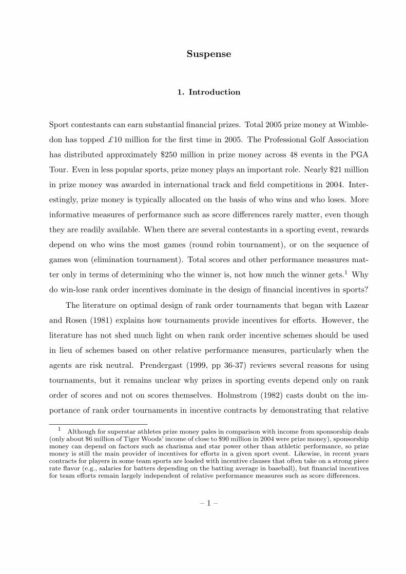
A rank order scheme rewards players entirely on the basis of who wins and who loses,

regardless of the score difference at the end. Such a scheme is represented by an “incentive

– 8 –

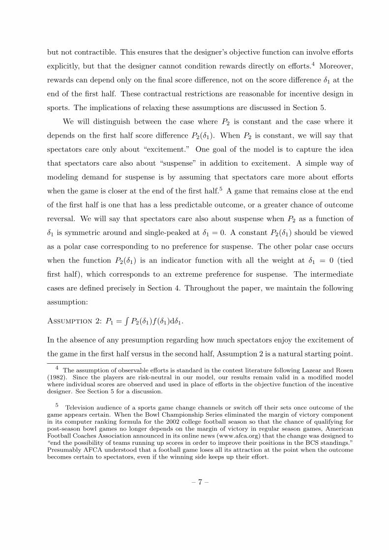
final score difference

reward

l

l+r

l+r 2

Figure 1. A rank order scheme

prize” r, which is the difference between the winner’s and the loser’s rewards, and a fixed

transfer l, which can be either positive or negative. See Figure 1 for an illustration. To find

the optimal rank order scheme, we use backward induction to characterize the equilibrium

response to an arbitrary rank order scheme (r, l).

In the second half, given first half score difference δ1, player A wins if δ2 is positive,

or δ1 + µA2 − µB

2 + ε2 > 0. The probability that A wins the game is therefore 1− F (−δ1 −µA

2 + µB2 ). Player A chooses µA

2 to maximize

r(1− F (−δ1 − µA2 + µB

2 ))− C(µA2 ),

where µB2 is taken as given. The necessary first order condition for A is

C ′(µA2 ) = rf(−δ1 − µA

2 + µB2 ).

Given the same first half score difference δ1, player B wins the game if δ2 is negative, which

occurs with probability F (−δ1 − µA2 + µB

2 ). Therefore, the first order condition for B is:

C ′(µB2 ) = rf(−δ1 − µA

2 + µB2 ).

The above two first order conditions imply that µA2 = µB

2 regardless of the first half score

difference δ1. That is, in equilibrium the leading player (player A if δ1 > 0 and B if δ1 < 0)

and the trailing player choose the same level of effort. This result is due to the fact that in

the second half the marginal benefit of effort, in terms of increased probability of winning,

is the same for the winning player and for the losing player.6

6 We note that the same result obtains even if the noise density function f is asymmetric. Also, itextends to a model with more than two periods. However, with more than two periods, equilibrium effortbefore the last period is no longer the same for the winning player and the losing player. See the discussionin Section 5.

– 9 –

Let µ2 be the players’ common equilibrium second half effort. It satisfies:

(1) C ′(µ2) = rf(δ1).

Since C is convex with C ′(0) = 0 and C ′(∞) = ∞, the above condition determines a unique

µ2 for any δ1 and r, denoted as µ2(δ1, r). As a function of δ1, the equilibrium effort µ2 is

symmetric around 0 because f is. This means that an individual player’s equilibrium effort

choice in the second half is the same whether after the first half the player is leading by

some score difference δ1 or trailing by the same score difference. Further, taking derivative

of the equilibrium condition (1), we have

∂µ2

∂δ1(δ1, r) =

rf ′(δ1)C ′′(µ2)

.

Since C is convex, under our assumption that f is single-peaked at δ1 = 0, the sign of

∂µ2/∂δ1 is determined by f ′, the slope of the density function: ∂µ2/∂δ1 is positive if δ1 < 0

and negative if δ1 > 0. This means that the second half equilibrium effort increases if the

score difference δ1 gets closer to 0 and decreases if δ1 drifts away from 0.7

The state of the game at the beginning of the second half is summarized by δ1, so we

can write the equilibrium payoff of each player at the beginning of the second half as

v(δ1) = rF (δ1)− C(µ2(δ1, r)) + l.

Taking derivative and using the equilibrium condition (1) for µ2, we have

(2) v′(δ1) = rf(δ1)− rf(δ1)∂µ2

∂δ1(δ1, r).

In the first half, player A chooses µA1 to maximize

∫v(µA

1 − µB1 + ε1)f(ε1)dε1 − C(µA

1 ),

where µA1 − µB

1 + ε1 represents the score difference δ1 at the end of the first half, and µB1

is taken as given. In the symmetric equilibrium, both players exert the same effort µ1 in

the first half, which satisfies the following necessary condition:

C ′(µ1) =∫

v′(ε1)f(ε1)dε1.

7 Ehrenberg and Bognanno (1990) document this dynamics of efforts in golf tournaments.

– 10 –

By the symmetry of µ2(δ1, r), the integral of the second term in v′(δ1) (equation 2) vanishes,

and the equilibrium condition for the first half can be simplified as

(3) C ′(µ1) =∫

rf2(ε1)dε1.

Thus, the first half effort is chosen as in a static game with a noise term equal to the sum

of the noise in the two halves. Given that the two players exert the same effort µ1 in the

first half, the equilibrium score difference δ1 is a random variable with the distribution

function F . In what follows, we continue to write µ2(δ1, r) instead of µ2(ε1, r), to stress

that µ2 depends on δ1, even though in equilibrium δ1 is equal to ε1.8

We can now compare equilibrium efforts µ1 and µ2. Our first result shows that in a

rank order scheme, the second half can be more exciting than the first half in terms of

generating greater efforts from the two players, but on average the second half gets boring.

Equilibrium dynamics of efforts are characterized in the following lemma.

Lemma 1. In a rank order scheme, the second half efforts are higher (lower) than the first

half efforts when the first half score difference is small (large), but the expected second

half efforts are at most as high as the first half efforts.

Proof: Compare the equilibrium conditions (1) and (3). Since µ2(δ1, r) is symmetric

around and single-peaked at δ1 = 0, so is C ′(µ2(δ1, r)) (as a function of δ1). Because (1)

and (3) imply

C ′(µ1) =∫

C ′(µ2(δ1, r))f(δ1)dδ1,

there exists some d > 0 such that C ′(µ1) > C ′(µ2(δ1, r)), and hence µ1 > µ2(δ1, r), if

and only if δ21 < d2. Further, Assumption 1 implies that C ′ is convex, and so by Jensen’s

inequality we have

C ′(µ1) ≥ C ′(∫

µ2(δ1, r))f(δ1)dδ1

).

8 Later we will show that under any linear score difference scheme, the first half score difference isalso equal to the random noise. Thus, which scheme is used does not directly affect the score difference.Our main theorem that rank order schemes dominate linear score difference schemes when spectators careabout suspense sufficiently does not result because rank order schemes induce closer scores. However,when the game is modeled with more than two periods, the score difference is no longer pure noise undera rank order scheme. See the discussion in Section 5.

– 11 –

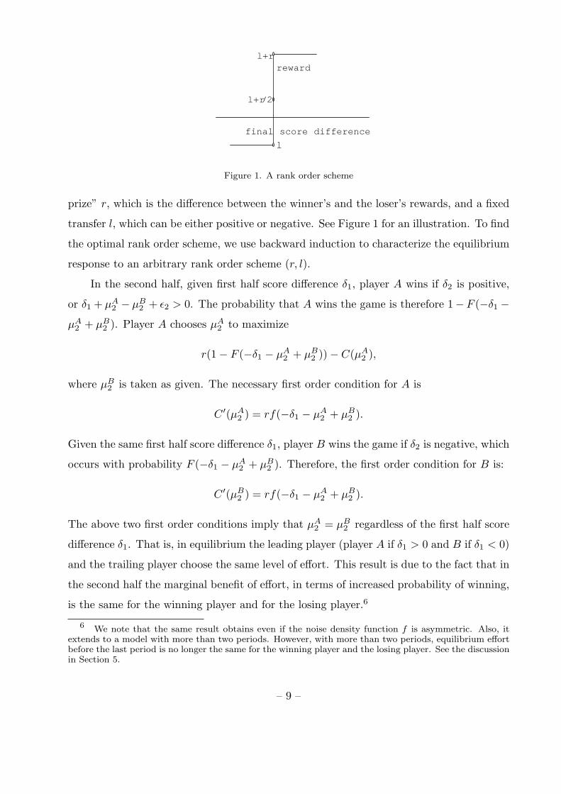
final score difference

reward

ts

Figure 2. A linear score difference scheme

Thus, µ1 ≥∫

µ2(δ1, r)f(δ1)dδ1. Q.E.D.

The incentive designer chooses the rank order scheme (r, l) to maximize “profits” per

player:

maxr,l

P1µ1 +∫

P2µ2(δ1, r)f(δ1)dδ1 −(

l +12r

)

subject to the participation constraint

l +12r − C(µ1)−

∫C(µ2(δ1, r))f(δ1)dδ1 ≥ U,

where µk, k = 1, 2, are equilibrium effort functions defined in equations (1) and (3). Since

the equilibrium efforts in the two halves depend only on r and not on l, the above optimiza-

tion problem is solved by first choosing r, which determines µ1 and µ2, and then choosing

l to bind the participation constraint. The optimal r satisfies the following necessary first

order condition:

(4)(P1 − C ′(µ1)

)dµ1

dr+

∫ (P2 − C ′(µ2(δ1, r))

)∂µ2

∂r(δ1, r)f(δ1)dδ1 = 0.

Assumption 1 ensures that the second order condition is satisfied.9

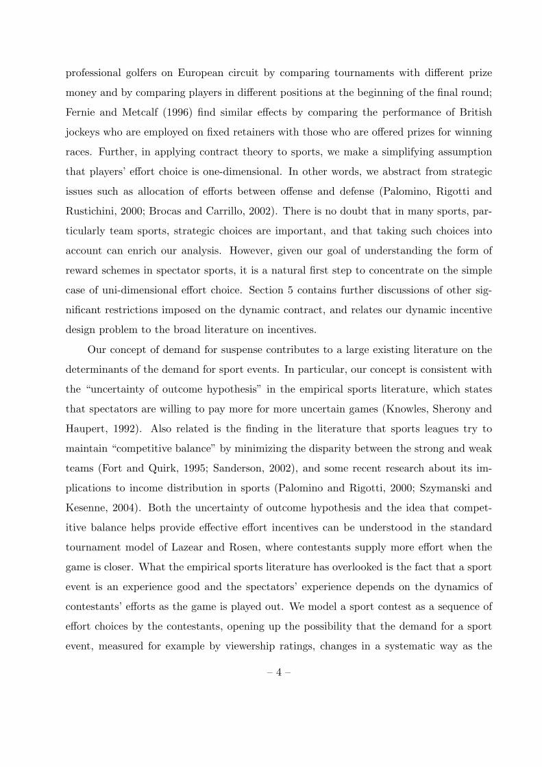
Next, we consider the optimal linear score difference scheme. A linear scheme has two

parameters: the fixed transfer t, which can be either positive or negative, and a piece rate

9 To see this, write the objective function as the difference between revenue i(r) and cost k(r), where

i(r) = P1µ1 +∫

P2µ2(δ1, r)f(δ1)dδ1, and k(r) = U + C(µ1) +∫

C(µ2(δ1, r))f(δ1)dδ1. The first order

condition for the optimal r is i′(r) = k′(r), and the second order condition is i′′(r) < k′′(r). A sufficientcondition for the second order condition is that i′′(r) ≤ 0 and k′′(r) ≥ 0 for all r, with at least one strictinequality. Using the equilibrium conditions for µ2(δ, r) and µ1 (equations 1 and 3), we can show thatunder the assumption that C′′′ ≥ 0, these efforts are weakly concave in r, and so i′′(r) ≤ 0. Similarly,the assumption that C′′′ ≤ (C′′)2/C′ implies that the effort cost in each half as a function of r is weaklyconvex, and so k′′(r) ≥ 0.

– 12 –

s. If the final score difference is δ2, then A’s reward is t + sδ2 and B’s reward is t − sδ2.

See Figure 2 for an illustration.

Under linear score difference schemes, the level of effort is the same for the two players

and for the two halves, and independent of the first half score difference. To see this, fix a

linear score difference scheme (t, s). Given the score difference δ1 at the beginning of the

second half, player A chooses µA2 to maximize

∫(t + s(µA

2 − µB2 + ε2 + δ1))f(ε2)dε2 − C(µA

2 ),

where µB2 is taken as given. Given symmetry, the same second half effort µ2 satisfies the

necessary condition:

(5) C ′(µ2) = s.

The equilibrium effort level µ2 is a constant determined entirely by the piece rate s. The

equilibrium payoff of each player at the beginning of the second half is therefore

v(δ1) = t + sδ1 − C(µ2).

In the first half, anticipating this equilibrium payoff, player A chooses µA1 to maximize

∫v(µA

1 − µB1 + ε1)f(ε1)dε1 − C(µA

1 ),

where µA1 − µB

1 + ε1 represents the random score difference δ1 at the end of the first half,

and µB1 is taken as given. In equilibrium both players exert the same effort µ1 in the first

half, which satisfies the following necessary condition:

C ′(µ1) =∫

v′(ε1)f(ε1)dε1.

Since v′ = s, the first order condition for the first half is the same as (5).

A constant level of effort µ, determined by C ′(µ) = s, is exerted by the two players

throughout the game. Given this, the designer’s profit maximization problem for the

optimal linear score difference scheme is

maxt,s

(P1 + P2)µ− t

– 13 –

subject to the participation constraint

t− 2C(µ) ≥ U.

The optimal piece rate s is given by 12 (P1 + P2), and the fixed transfer t binds the partic-

ipation constraint.

A rank order scheme on average gets boring (generates low efforts from players) in

the second half, but can become exciting when the game is close at the end of the first

half. In contrast, under a linear score difference scheme, players keep up the same level of

effort regardless of whether the game is close or lopsided after the first half. How do the

two schemes compare if both are chosen optimally?10

Proposition 1. When spectators care only about excitement, the optimal linear score

difference scheme dominates all rank order schemes.

Proof: Let (r, l) be the optimal rank order scheme, and let µ1 and µ2(δ1, r) be the

equilibrium efforts. Define µ = 12 (µ1 +

∫µ2(δ1, r)f(δ1)dδ1). Then, since C is convex,

C(µ1) +∫

C(µ2(δ1, r))f(δ1)dδ1 ≥ C(µ1) + C

(∫µ2(δ1, r)f(δ1)dδ1

)≥ 2C(µ).

From Assumption 2,

P1µ1 + P2

∫µ2(δ1, r)f(δ1)dδ1 = (P1 + P2)µ.

Define s = C ′(µ). Then a linear scheme with the piece rate s induces µ, with a lower effort

cost to the players and the same revenue to the designer. Define t = U +2C(µ), then (t, s)

generates greater profits than (r, l). Q.E.D.

The conclusion of Proposition 1 can be strengthened by noting that the optimal linear

score difference scheme implements the first best efforts. The first best efforts maximize

the difference between the revenue and the cost

P1µ1 +∫

P2µ2(δ1)f(δ1)dδ1 − C(µ1)−∫

C(µ2(δ1))f(δ1)dδ1 − U.

10 The proof remains valid if Assumption 2 is replaced by the weaker condition P1 ≤ P2. By Lemma 1,if P1 is sufficiently greater than P2, then the result of Proposition 1 is reversed. We ignore this possibilityas it seems unreasonable in sports tournaments.

– 14 –

The first order necessary conditions for the first best efforts µ∗1 and µ∗2 are therefore

(6)C ′(µ∗1) = P1;

C ′(µ∗2) = P2.

Under Assumption 2, the optimal linear scheme with s = 12 (P1 + P2) achieves the first

best.

4. Excitement and Suspense

Given the importance of rank order incentives in the design of financial incentives in sports,

the inferiority of rank order schemes to score difference schemes established in the previous

section calls for an explanation. Our attempt is motivated by the unique feature in sports

that spectators care about the dynamics of the game. We model this by assuming that

spectators value player’s efforts more when the game is closer. Formally, we assume that P2

depends on δ1. In particular, P2(δ1) is symmetric around and single-peaked at δ1 = 0 (tied

first half). This modification of spectators’ preference captures the idea that spectators

enjoy both excitement and suspense. Spectators do not care about excitement only: a lop-

sided game is not appealing even when the losing side keeps up the effort. On the other

hand, spectators do not care about suspense only: they do not like it when the leading

player slacks off even though it makes the game close. We show in this section that rank

order schemes perform better than score difference schemes when spectators have a strong

enough preference for suspense.

We capture the concept of increasing demand for suspense by assuming that P2 is

indexed by a one-dimensional parameter a, such that, with a slight abuse of notation, the

demand for suspense is greater under P2(δ1, a) than under P2(δ1, a) when a > a. The

functions P2(δ, a) satisfy: (i)∫

(P2(δ1, a) − P2(δ1, a))f(δ1)dδ1 = 0 for any a and a, and

(ii) there exists a function α(a) such that ∂P2(δ1, a)/∂a > 0 if and only if δ21 < α2(a).

We say that P2(δ1, a) is more “concentrated” (with respect to f) than P2(δ, a) if a > a.

Intuitively, P2(δ1, a) is more concentrated in the sense that the two functions have the same

expectation under density f , but the value of P2(δ1, a) is larger for close games (middle

– 15 –

values of δ1) and smaller when a player has acquired a strong lead (more extreme values

of δ1 in either direction).

Increasing demand for suspense does not change the design of linear difference scheme.

Since the two players exert the same effort in the two halves regardless of the score dif-

ference, the optimal piece rate s depends only on the expectation of P2(δ1), which does

not change. The fixed transfer t that binds the player’s participation constraint is also

unchanged. In contrast, intuition suggests that the optimal rank order scheme should

change as spectators’ demand for suspense increases. As P2(δ1) becomes more concen-

trated around δ1 = 0, the designer will want to make µ2(δ1, r) also more concentrated in

order to take advantage of the fact that spectators have a greater demand for suspense.

How can this be achieved? From the equilibrium condition for second half effort µ2, we

see that increasing r will raise µ2(δ1, r) for all δ1. But since the density function f(δ1) is

uni-modal, the increase in µ2 will be more pronounced around δ1 = 0. Thus, as P2(δ1)

becomes more concentrated around δ1 = 0, the designer will want to increase r. This

intuition is confirmed in the following result.

Lemma 2. As demand for suspense increases, the incentive prize under the optimal rank

order scheme increases and the optimal profits also increase.

Proof: From the equilibrium condition for second half effort µ under rank order scheme

(equation 1), we find that∂µ2

∂r(δ1, r) =

f(δ1)C ′′(µ2(δ1, r))

.

Since both f(δ1) and µ2(δ1, r) are symmetric around δ1 = 0, ∂µ2(δ1, r)/∂r is also symmet-

ric. Furthermore,∂2µ2

∂r∂δ1(δ1, r) = f ′(δ1)

(C ′′)2 − C ′′′C ′

(C ′′)3.

Under Assumption 1, ∂µ2(δ1, r)/∂r is also single-peaked around δ1 = 0.

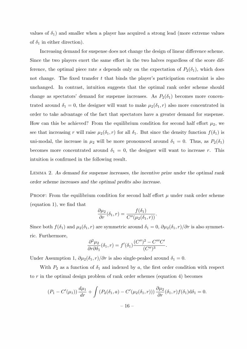
With P2 as a function of δ1 and indexed by a, the first order condition with respect

to r in the optimal design problem of rank order schemes (equation 4) becomes

(P1 − C ′(µ1))dµ1

dr+

∫(P2(δ1, a)− C ′(µ2(δ1, r)))

∂µ2

∂r(δ1, r)f(δ1)dδ1 = 0.

– 16 –

Taking derivatives of the above condition with respect to a, we find that, dr/da, the effect

of increasing demand for suspense, has the same sign as∫

∂P2

∂a(δ1, a)

∂µ2

∂r(δ1, r)f(δ1)dδ1.

By condition (i) of increasing demand for suspense,∫

(∂P2(δ1, a)/∂a)f(δ1)dδ1 = 0. Then,

for any constant α we can write the above integral as∫

∂P2

∂a(δ1, a)

(∂µ2

∂r(δ1, r)− ∂µ2

∂r(α, r)

)f(δ1)dδ1.

By condition (ii) of the definition of increasing demand for suspense, we can choose α > 0

such that ∂P2(δ1, a)/∂a is positive for all δ1 ∈ (−α, α), and negative for any δ1 < −α

or δ1 > α. We have shown that ∂µ2(δ1, r)/∂r is symmetric around and single-peaked at

δ1 = 0. Then, the above integral is positive both for δ1 < −α and for δ1 > α, because

∂P2(δ1, a)/∂a < 0 and ∂µ2(δ1, r)/∂r < ∂µ2(α, r)/∂r. The integral from −α to α is also

positive because ∂P2(δ1, a)/∂a > 0 and ∂µ2(δ1, r)/∂r > ∂µ2(α, r)/∂r. It follows that

dr/da > 0.

By the envelope theorem, the change in the value of the objective function under the

optimal rank order scheme has the same sign as∫

∂P2

∂a(δ1, a)µ2(δ1, r)f(δ1)dδ1.

We know that µ2(δ1, r) is symmetric and single-peaked, just like ∂µ2(δ1, r)/∂r. By a

similar argument as above, the above integral is positive, and therefore the value of the

objective function under the optimal rank order scheme increases. Q.E.D.

Similar comparative statics about the design and the profits of the optimal rank order

scheme can be carried out with respect to the density function f of the noise in the

game. A more concentrated f represents an environment of sports competition that is

less susceptible to pure luck of players, and therefore more responsive to their efforts in

the game.11 Comparative statics with respect to the role of chance is interesting because

11 In our model, performance measurement errors decrease the likelihood that the score will stay closein the second half and reduce the utility of the spectators. In the standard principal-agent moral hazardliterature, measurement errors increase the risk premium of the agent. In both cases, measurement errorsdecrease profits by hampering the working of incentive contracts.

– 17 –

characteristics of a sports game can be, and indeed have often been, modified when changes

are introduced to the rules of the game, training technology for athletes, or equipment used

in the game. Formally, we can define “diminishing role of chance” in the game as follows.

Let the density function f of the noise be indexed by a one-dimensional parameter b, such

that there exists a function β(b) with ∂f(δ1, b)/∂b > 0 if and only if δ21 < β2(b). This

condition means that f becomes more concentrated for middle values of δ1. Intuitively,

when f becomes more concentrated, the game is more likely to be closer given any effort

levels of the two players, and the incentive designer should respond by increasing the

incentive prize, in the same way as when P2 becomes more concentrated. Indeed, the proof

of Lemma 2 can be directly extended to show that with a diminishing role of chance (that

is, as b increases), the incentive designer increases the incentive prize and the profits under

the optimal scheme also increase. Thus, diminishing role for chance has the same effects

on the design and the profits of the optimal scheme as increasing demand for suspense.12

We want to show that when spectators care enough about suspense in the game,

the optimal rank order scheme eventually dominates the optimal linear score difference

scheme. We establish this result indirectly, by noting that there is a rank order scheme

that achieves the first best efforts in both halves if and only if f(δ1)/P2(δ1) is constant for

all δ1. The conditions for the first best efforts in the two halves are given by equations

(6) in Section 3, with P2 replaced by P2(δ1). These conditions can be replicated by the

equilibrium conditions (1) and (3) under a rank order scheme, if and only if f(δ1)/P2(δ1)

is constant for all δ1.13

12 There is an important difference between the comparative statics with respect to P2 and withrespect to f . In the case of increasing demand for suspense, the design and the profits of the optimallinear score difference schemes are not affected, and therefore the relative advantage of rank order schemesemerges. In the case of diminishing role of chance, one can show that the optimal piece rate s in a linear

score difference scheme is given by 12(P1 +

∫P2(δ1)f(δ1, b)dδ1), which increases with b. Similarly, the

effect of increasing b on the profits under the optimal linear score difference scheme has the same sign

as µ(s)∫

P2(δ1)(∂f(δ1, b)/∂b)dδ1 (where µ(s) is defined by C′(µ(s)) = s), which can be shown to be

positive. Thus, with diminishing role of chance, performance is improved under both the optimal rankorder difference scheme and the optimal linear score difference scheme. The net effect on the comparison ofthe two schemes is generally ambiguous. Note that in the above comparative statics exercise with respectto f , Assumption 2 is no longer satisfied.

13 The role of Assumption 2 is now apparent. When the assumption is not satisfied, no reward schemesbased on final score difference, including rank order schemes and linear score difference schemes, canimplement the first best efforts. This follows because the equilibrium conditions for the first best first halfefforts and the second half efforts cannot be satisfied at the same time. Intuitively, under our assumption

– 18 –

Now we are ready to show that rank order schemes dominate linear score difference

schemes when spectators’ demand for suspense is sufficiently high. Consider the problem of

designing the optimal rank order scheme, for a given preference function P2(δ1). For sim-

plicity, we assume that the rescaled functions P2(δ1)/P1 and f(δ1)/(∫

f2(x)dx) intersect

exactly twice, at d and −d. For the following result, we say that the demand for suspense

is high relative to the chance in the game, if P2(δ1)/P1 > f(δ1)/(∫

f2(x)dx) when δ21 < d2

(i.e., if P2(δ1) is more concentrated than f(δ1) after proper rescaling.)

Proposition 2. If spectators’ demand for suspense is high relative to the chance in the

game, then the optimal rank order scheme dominates all linear score difference schemes.

Proof: Consider a class of spectator preference functions P2(δ1, a) indexed by a, given by

P2(δ1, a) =P1f(δ1)∫f2(x)dx

+ a

(P2(δ1)− P1f(δ1)∫

f2(x)dx

).

By construction,∫

(∂P2(δ1, a)/∂a)f(δ1)dδ1 = 0, so condition (i) of increasing demand for

suspense is satisfied. By assumption, ∂P2(δ1, a)/∂a is positive if and only if δ21 < d2 for

all a, so condition (ii) of increasing demand for suspense is also satisfied. Since P2(δ1, 0) is

proportional to f(δ1), at a = 0 the optimal rank order scheme achieves the first best and

therefore dominates linear schemes. Lemma 2 then implies that the optimal rank order

scheme continues to dominate linear schemes when a = 1. But this is precisely what we

need, because P2(δ1, 1) = P2(δ1) by construction. Q.E.D.

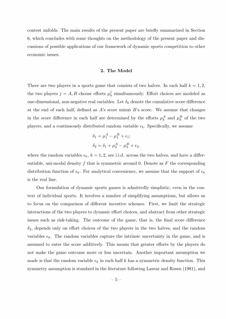
Proposition 2 can be strengthened. The continuity of the profits under the optimal

rank order scheme in a implies that the conclusion of Proposition 2 can hold even if specta-

tors’ demand for suspense is “a little” lower than the chance in the game. More precisely,

since when P2(δ1) is proportional to f(δ1), the optimal rank order scheme implements

the first best efforts and therefore dominates linear score difference schemes, if the given

P2(δ1) is just a little less concentrated than f(δ1), the optimal rank order scheme still

that the reward for the players depends only on the final score difference, the incentives for the first halfand for the second half are directly linked (e.g., through equations (1) and (3) under a rank order scheme).When Assumption 2 is not satisfied, such link becomes a binding restriction on what can be achievedunder a reward scheme based on the final score difference.

– 19 –

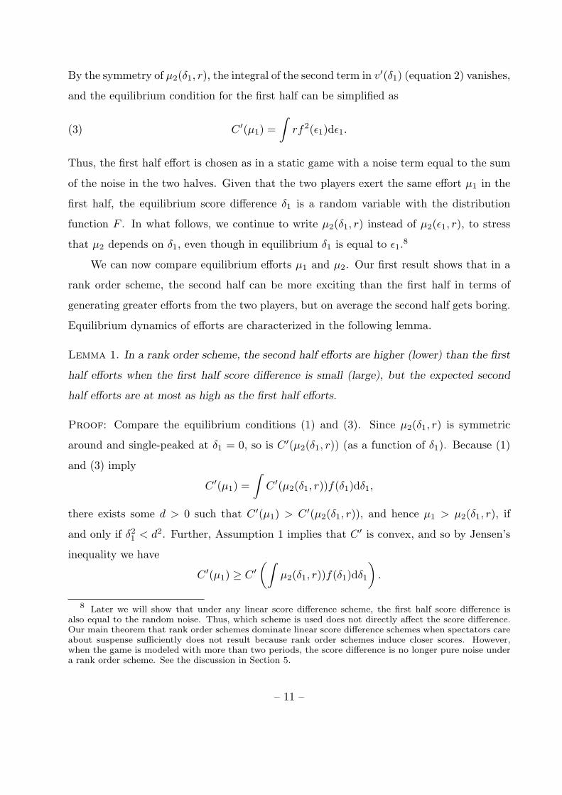
0.5 1 1.5 2

0.95

1.05

1.1

1.15

hp hf

demand for suspense

relative

performance

Figure 3. Relative performance: rank order and linear score difference

dominates linear score difference schemes. Figure 3 illustrates the case where the effort

cost function is C(µ) = 12µ2, and both the rescaled preference function P2 and the noise

density function f are normal, with precision (inverse of variance) hp and hf respectively.

The curve represents the ratio of the profit under the optimal rank order scheme to the

profit under the optimal linear scheme, as a function of hp/hf . Note that the optimal rank

order scheme outperforms the optimal linear scheme even when the demand for suspense

falls well under what it takes to make the optimal rank order scheme achieve the first best

(i.e. when hp/hf = 1).

Propositions 1 and 2 give us a clear picture of the comparison between linear score

difference schemes and rank order schemes. Linear schemes dominate when the demand

for suspense is low, while rank order schemes dominate when the demand is high. Indeed,

linear schemes and rank order schemes stand at the opposite ends of a continuum: a linear

scheme provides constant incentives to increase the final winning margin, while a rank

order scheme provides no incentive at all at the margin so long as winning is ensured. The

former achieves the first best when there is no demand for suspense (P2(δ1) is independent

of δ1), while the latter achieves the first best when the demand for suspense matches the

randomness in the game (P2(δ1) is proportional to f(δ1)). One can imagine that there

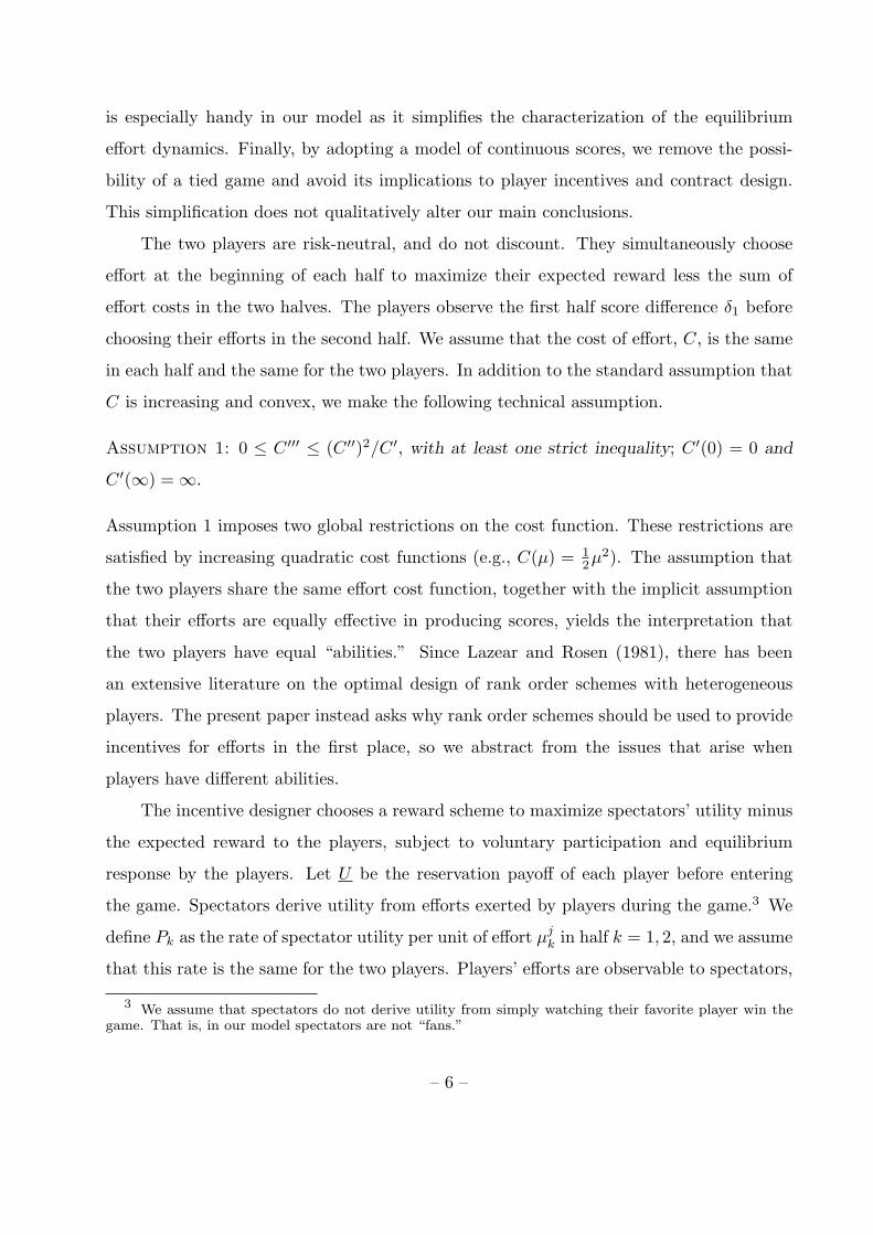
are other schemes based on the final score difference that provide incentives intermediate

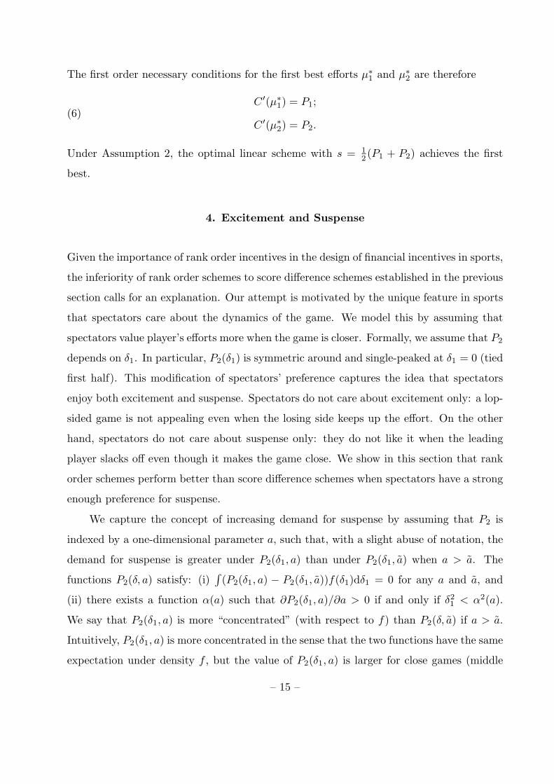
between those under the piece rate and the rank order tournament. Figure 4 illustrates

a family of such schemes generated by normal distribution functions of different precision

(and zero mean). A natural question to ask is then: can these schemes achieve the first

best where linear schemes and rank order schemes fail?

– 20 –

final score difference

reward

Figure 4. Nonlinear score difference schemes

To understand how linear schemes and rank order schemes compare with other schemes

based on the final score difference, we begin with the question of whether the first best

efforts can be implemented outside the two polar cases known from Propositions 1 and

2, namely, when there is no demand for suspense (P2(δ1) is independent of δ1) and the

optimal linear scheme achieves the first best, and when the demand for suspense matches

the role of chance (P2(δ1) is proportional to f(δ1)) and the optimal rank order scheme

achieves the first best. Consider the class of nonlinear schemes n based on the final score

difference δ2. For analytical convenience, we restrict our attention to functions n(δ2) that

are differentiable, with derivatives n′ that are symmetric around and single-peaked at

δ2 = 0. We refer to n as a “nonlinear” scheme, although nonlinear schemes include linear

schemes as a special case with a constant n′, and rank order schemes as a limit case with n′

arbitrarily close to an indicator function with all weights on the point of δ2 = 0. Following

the previous analysis, we can establish the equilibrium effort condition in the first half:

(7) C ′(µ1) =∫ ∫

n′(δ1 + ε2)f(ε2)dε2f(δ1)dδ1,

and the condition in the second half:

(8) C ′(µ2(δ1)) =∫

n′(δ1 + ε2)f(ε2)dε2.

Compare these conditions to those for the first best efforts (equations 6). A nonlinear

score difference scheme n(δ2) implements the first best efforts in both halves if and only if

for all δ1,

(9)∫

n′(δ1 + ε2)f(ε2)dε2 = P2(δ1).

– 21 –

The above equation may not have a solution for the function n′ for given noise density

function f and the preference function P2.

We may think of the functions f and rescaled n′ and P2 as density functions of random

variables X, Y and Z respectively. Then condition (9) means that for the nonlinear scheme

n to achieve the first best, n′ is such that the random variable Z is the convolution of X

and Y (i.e., the sum of independent random variables X and Y ). This suggests that for

certain specifications of the density function f and the preference function P2(δ1), explicit

forms of the nonlinear scheme that induces the first best efforts can be found. Suppose

that both f and P2 (after proper rescaling) are normal, with mean 0 and precision hf and

hp respectively. Then, the nonlinear scheme n achieves the first best if n′ is proportional to

the normal density function with mean 0 and precision (h−1p −h−1

f )−1, as long as hp < hf .

For any fixed hf , as hp increases to hf , the optimal nonlinear reward function n converges

to a rank order scheme. In the limiting case of hp = hf , the rank order scheme achieves

the first best efforts. This result serves as a special case of Proposition 2. If hp > hf ,

there is no reward function n that achieves the first best. The demand for suspense is too

high relative to the noise distribution, and even rank order schemes fail to limit players’

incentives in the second half when the game becomes lop-sided at the end of the first half.

In this case the designer wants to reduce the incentives for continuing second half efforts

to a minimum when the first half score difference is sufficiently large. Since rank order

schemes give no reward to the winner for the margin of victory, one naturally conjectures

that the optimal rank order scheme achieves the second best among all schemes based on

the final score difference, but additional assumptions are necessary to validate the intuition.

We focus on the “normal-quadratic” case, where the noise density function is normal

with mean 0 and precision hf , the preference function is proportional to a normal density

function with mean 0 and precision hp, and the effort cost function is quadratic. The

following proposition assumes that hp > hf . By a “normal” scheme we mean any nonlinear

scheme n such that n′ is proportional to a zero-mean density function up to a constant.

Proposition 3. If spectators’ demand for suspense is high relative to the chance in the

game, then in the normal-quadratic case the optimal rank order scheme dominates any

normal incentive scheme.

– 22 –

Proof: Without loss of generality, assume that C(µ) = 12µ2. First consider the class

of differentiable schemes with symmetric derivatives, which includes schemes that provide

normal incentives. Suppose that a scheme n is optimal in the class. Then, n maximizes

the profit

P1µ1 +∫

P2(δ1)µ2(δ1)f(δ1)dδ1 − 12µ2

1 −∫

12µ2

2(δ1)f(δ1)dδ1 − U,

subject to the equilibrium conditions for efforts (equations 7 and 8). Consider an alter-

native scheme n(δ2) = n(δ2) + Kδ2. Since n is optimal, the derivative of the profit with

respect to K vanishes at K = 0:

(10) P1 +∫

P2(δ1)f(δ1)dδ1 − µ1 −∫

µ2(δ1)f(δ1)dδ1 = 0.

The equilibrium effort conditions (equations 7 and 8) imply∫

µ2(δ1)f(δ1)dδ1 = µ1.

Therefore, under Assumption 2 equation (10) implies µ1 = P1 and

(11)∫

µ2(δ1)f(δ1)dδ1 = P1.

As a result, the scheme n maximizes

(12)∫

P2(δ1)µ2(δ1)f(δ1)dδ1 −∫

12µ2

2(δ1)f(δ1)dδ1

subject to equations (11) and (8).

Now suppose that the optimal scheme n provides normal incentives for efforts. Let

hn′ be the precision of the normal density function corresponding to n′. Since f is normal,

equation (8) implies that up to some constant the equilibrium second half effort function

µ2(δ1) under n is also proportional to a zero-mean normal density function. Let hµ be

the precision of the corresponding normal density function. Then equation (8) implies

that h−1µ = h−1

n′ + h−1f . Thus, hµ < hf and hµ increases with hn′ . Since by hf < hp by

assumption, we have hµ < hp. Consider the effect on the second half profit (equation 12)

of making µ(δ1) more concentrated. This effect is given by the following derivative:

(13)∫

∂µ2(δ1)∂hµ

(P2(δ1)− µ2(δ1))f(δ1)dδ1.

– 23 –

Since hµ < hp, equation (11) implies that P2(δ1)− µ2(δ1) is symmetric and single-peaked.

Moreover, ∂µ2(δ1)/∂hµ is also symmetric and single-peaked. An argument similar to the

proof of Lemma 2 then implies that the derivative (equation 13) is positive. Since hµ

increases with hn′ , we have established that the incentive designer can increase profit by

increasing hn′ . This contradicts the assumption that n is optimal among all schemes that

provide normal incentives. The proposition follows immediately from the fact that hµ

achieves the greatest possible value of hf under a rank order scheme. Q.E.D.

Now we briefly comment on the restrictions imposed in Proposition 3. The assump-

tion of quadratic effort cost function allows us to obtain explicit functional forms for the

equilibrium efforts. More importantly, together with Assumption 2, the quadratic cost

assumption enables us to use a variational method to separate profit maximization in the

two halves. Without this assumption, the marginal cost of effort is nonlinear. Instead of

equation (10), we have

P1

C ′′(µ1)+

∫P2(δ1)

C ′′(µ2(δ1))f(δ1)dδ1 − C ′(µ1)

C ′′(µ1)−

∫C ′(µ2(δ1))C ′′(µ2(δ1))

f(δ1)dδ1 = 0.

Equilibrium efforts in the two halves cannot be separated, and optimal nonlinear schemes

would in general trade off the first half effort against the second half effort. The normality

restriction for the noise density function, the preference function and the nonlinear schemes

reduces the comparison among f , P2 and different nonlinear schemes n to a one-dimensional

parameter, and allows us to examine the effect on the second half profit (equation 12)

through µ2(δ1), instead of through n′ and equation (8). As an alternative to the normality

restriction, one could imagine that there is a one-dimensional parameter, say i, which

indexes f , P2 and n′, with a greater value of i implying greater concentration. But in

general µ2(δ1) as determined by equation (8) as a convolution of n′ and f is not indexed

by the same parameter i.14 This makes it impossible to evaluate the effect of making

µ2(δ1) more concentrated on the second half profit (equation 13).

14 The convolution of two symmetric and single-peaked functions is always symmetric and single-peaked, but even if the original two functions are ordered according to some one-dimensional parameter,the result of convolution in general cannot be compared in terms of concentration. To see this, supposethat g1 and g2 are symmetric and single-peaked (around 0), and let g be the convolution of the two, given

by g(x) =∫

g1(x + y)g2(y)dy. Symmetry of g can be shown by a change of variable. Single-peakedness

– 24 –

5. Discussions

In our model of sports games individual scores play no role in the design of incentive

schemes; only score differences matter. Since in most sports individual scores are observable

and verifiable, one may wonder whether our results are robust if individual scores are used

in incentive schemes. To address this issue, we need to modify our model. Suppose that

θj1 is the first half score of player j = A, B, determined according to:

θj1 = µj

1 + ηj1,

where ηj1 is a random variable. The second half score θj

2 is determined similarly:

θj2 = θj

1 + µj2 + ηj

2.

Let δi = θAi − θB

i be the score difference for each half i. We assume that ηji ’s are i.i.d.

(across players and across time), with the distribution function H. To facilitate comparison

with earlier results, we maintain the other main assumption on the incentive contracts:

rewards to each player can depend only on the final scores θA2 and θB

2 . Assume also the

designer’s objective function is the same as in Section 4.15

The question we want to answer is whether there is any loss of generality to restrict

incentive schemes to those conditioned on score differences.. However, the opposite ques-

tion seems more immediate: why should player A’s incentive depend on B’s performance

at all? The answer is clearly that it should not if P2 is constant. That is, when there is no

demand for suspense, the two players should be independently rewarded according to their

follows from the result that∫

g′1(x + y)g2(y)dy < 0 if and only if x > 0 (write the integral as the sum of∫y≥x

g′1(y)(g2(y − x)− g2(y + x))dy and∫0≤y<x

g′1(y)(g2(y − x)− g2(y + x))dy; both parts are negative

because single-peakedness of g1 implies g′1(−y) = −g′1(y) > 0 for any y > 0.) Further, if g1 becomesmore concentrated according to a parameter i, an argument similar to that in the proof of Lemma 2 shows

that∫

(∂g1(y)/∂γ)g2(y)dy increases with i, and therefore g(0) becomes greater. However, in general the

function g can change arbitrarily with i at other points, so that the concentration of g cannot be measuredaccording to i.

15 We note that in this alternative setup a player’s score is independent of the efforts of his opponent.There is hardly any sport where this is completely accurate. Even for non-confrontational sports suchas sprint and swimming, it makes a difference whether an athlete is performing by himself or competingagainst other athletes.

– 25 –

own scores. Of course, this is a just a special case of Holmstrom’s (1982) celebrated re-

sult that tournaments have no intrinsic value in providing incentives in a team production

problem, if individual output can be measured and measurement errors are independent.

In our dynamic model, the players are risk-neutral, so under Assumption 2 the argument

used in proving Proposition 1 shows that the first best efforts can be achieved with a pair

of individualized, linear incentive schemes. Clearly, the two individualized schemes are

identical, implying that a linear scheme based on the score difference achieves the first

best as well, which is precisely the import of Proposition 1. Thus, there is no reason to

tie the incentives of the two players together when there is no demand for suspense, but

symmetry and Assumption 2 imply that there is no loss of generality in using a scheme

based on score differences.

The situation is different when P2 is a function of δ1. Now, the objective function

of the incentive designer introduces a link between the incentives of the two players. But

we will argue that there is no loss of generality in assuming that the incentives for one

player depend on the final score of his opponent only through the final score difference. To

begin, let mj(θA2 , θB

2 ) be the reward scheme for player j = A,B. It is natural to assume

symmetry, with mA(θ, θ) = mB(θ, θ). As usual, we look at the equilibrium conditions in

the second half, given the first half scores θA1 and θB

1 (and hence δ1 = θA1 − θB

1 ). Player A

chooses µA2 to maximize

∫ ∫mA(θA

1 + µA2 + ηA

2 , θB1 + µB

2 + ηB2 )dH(ηA

2 )dH(ηB2 )− C(µA

2 ),

taking as given µB2 . This yields a necessary condition for player A’s best response function

in the second half: ∫ ∫∂mA

∂θA2

dH(ηA2 )dH(ηB

2 ) = C ′(µA2 ).

An analogous condition for player B holds. The symmetry assumption implies that the

incentives facing player A when the first half scores are (θ, θ) are the same as the incentives

facing player B when the scores are (θ, θ). The two conditions determine the second half

equilibrium efforts µA2 and µB

2 , which in general depend on both θA1 and θB

1 .

Relative to the nonlinear schemes n(δ2) analyzed in Section 4, a pair of individualized

schemes mA and mB can achieve second half equilibrium efforts that are more general

– 26 –

in two ways. First, for a given first half score difference δ1, the total score θA1 + θB

1

may differ, and (mA,mB) can create different incentives for the two players. Second,

for a given first half score difference δ1, the individualized scheme (mA,mB) can create

different incentives for the leading player and the trailing player.16 However, with the

preference function P2 depending only on the first half score difference, and the effort cost

function C being identical and convex, there is no reason for the designer to exploit these

new possibilities allowed by individualized schemes (mA,mB). An argument similar to

the proof of Proposition 1 shows that any individualized scheme (mA,mB) that creates

different incentives for the same first half score difference is dominated by another scheme

that homogenizes the incentives among different levels of total scores and between the two

players.

Another restriction we have imposed on the reward schemes is that they do not depend

on the first half score difference. This restriction is not binding when there is no demand

for suspense, as the first best efforts can be implemented with a linear scheme that depends

only on the final score difference (Proposition 1). This result is related to Holmstrom and

Milgrom’s (1987) theory of linear incentive contracts in a model of a single risk-averse agent

with no wealth effect in the utility function. They show that in a dynamic environment

in which the agent can adjust his efforts according to a commonly observed history of

output, the principal cannot do better than making the payment conditional only on some

aggregated output measure. In particular, the two-wage payment schemes proposed by

Mirrlees (1974) to approximate the first best do not work well because the agent can game

such schemes by conditioning his efforts on the output path. Our Proposition 1 establishes

a related result with a different logic in a multiple-agent setting. Rank order schemes

correspond to the two-wage payment schemes of Mirrlees, because the equilibrium effort

function in the second half depends on the first half score difference, while linear score

difference schemes correspond to linear contracts of Holmstrom and Milgrom, because the

incentives facing the players are constant throughout the game. Linear schemes dominate

16 This is impossible under any nonlinear scheme n with symmetric n′. Note also that the symmetryassumption imposed on (mA, mB) does not mean ∂mA(θA

2 , θB2 )/∂θA

2 = ∂mB(θA2 , θB

2 )/∂θB2 . Symmetry

means role reversal when the individualized scores are reversed not that the leading player faces the sameincentives as the losing player.

– 27 –

rank order schemes because constant incentives are cost-efficient in our setting, not because

the players can exploit the dependence of incentives on the history of the game.

When the demand for suspense is so high that no incentive scheme based on the final

score difference achieves the first best, one naturally suspects that the restriction to final

score difference schemes becomes binding. Indeed, we now show that the first best can

always be achieved with a “conditional” linear scheme in which the intensity of incentives

depends on the first half score difference. If a conditional linear scheme with a piece

rate s(δ1) and a fixed transfer t achieves the first best, then the second half equilibrium

condition for effort (equation 5) and the condition for first best second half effort (the

second equation in 6) must coincide. Thus,

s(δ1) = P2(δ1).

The equilibrium payoff function of each player at the end of the first half is therefore:

v(δ1) = t + P2(δ1)δ1 − C(µ∗2(δ1)),

where µ∗2(δ1) is the first best second half effort. This implies

v′(δ1) = P2(δ1) + P ′2(δ1)δ1 − C ′(µ∗2(δ1))dµ∗2(δ1)

dδ1.

The equilibrium condition for the first half effort is

C ′(µ1) =∫

v′(ε1)f(ε1)dε1.

Compare the above with the condition for the first best first half effort (the first equation in

6). For the conditional linear scheme with s(δ1) to achieve the first best, the expectation of

the second and third term in v′(δ1) must vanish. The third term does have a zero integral

with respect to f , because µ∗2(δ1) is symmetric with respect to 0. However, the expectation

of the second term in v′(δ1) is negative, because P ′2(δ1) is positive (negative) when δ1 is

negative (positive). Thus, if the piece rate s(δ1) of the conditional linear scheme is chosen

to make the second half effort the first best, the first half effort will be smaller than the

corresponding first best. The reason for this result is clear. For the second half effort to

– 28 –

be the first best, the piece rate of the linear scheme must be aligned with the preference

function P2. Through the effect on the first half score difference, the players anticipate

the impact of their first half effort on their reward. When choosing the first half effort,

players not only factor in the impact on their reward given the intensity of the incentives,

which is what the designer wants, but also the impact on their reward due to changes in

the intensity when the first half score difference changes, which is unwanted. The effect

of the unwanted anticipation by the players is negative on their first half effort, because a

greater first half score difference reduces the intensity of the incentives.

But this problem can be easily fixed, if the designer can also condition the fixed

transfer t on the first half score difference δ1. In this case, there is an additional term in

v′(δ1), which is t′(δ1), and the function t(δ1) can always be chosen to exactly cancel the

unwanted second term in v′(δ1). Other schemes can be conditioned on the first half score

difference to achieve the first best. For example, a similar analysis shows that a conditional

rank order scheme (l(δ1), r(δ1)) achieves the first best regardless of how concentrated P2

is relative to f . Again, it is essential that both the fixed transfer l and the incentive prize

r depend on δ1.

If conditional schemes help align players’ incentives to spectators’ interests, why are

such schemes seldom seen in practice? Conditional schemes are more difficult to administer

than schemes based on the final score differences. The gain from using conditional schemes

may not be significant enough to outweigh the inconvenience in their use. This is especially

true if the demand for suspense is not too high relative to the chance in the game, if

there are many periods in one game, or if there are frequent changes in scores, so that

aligning players’ incentives to spectators’ interests requires frequent fine-tuning of the

prizes throughout the game. A separate reason why complicated conditional schemes are

not used in practice may be that, when the demand for suspense is high relative to the

chance in the game, the incentive designer can use other tools to help the rank order scheme

manage players’ incentives according to the state of the game. One such tool is to stratify

the aggregation of points in the calculation of the final score difference. For example, in

a tennis match, points are aggregated into games, games into sets, and the first player to

win a given number of sets (three or five) wins the match and the winner’s purse. Similar

– 29 –

scoring schemes are used in volleyball and in playoff series in basketball. A related tool

is to end each period in a game or the entire game when the scores become lop-sided,

while prolonging the game when the score differences are small. Thus, a set in tennis can

be decided in six love-games, or it can continue indefinitely, at least theoretically, with

tie-breaking in each game. These tools are simple to administer, and can be effective in

economizing on incentives and aligning them to spectators’ interests.

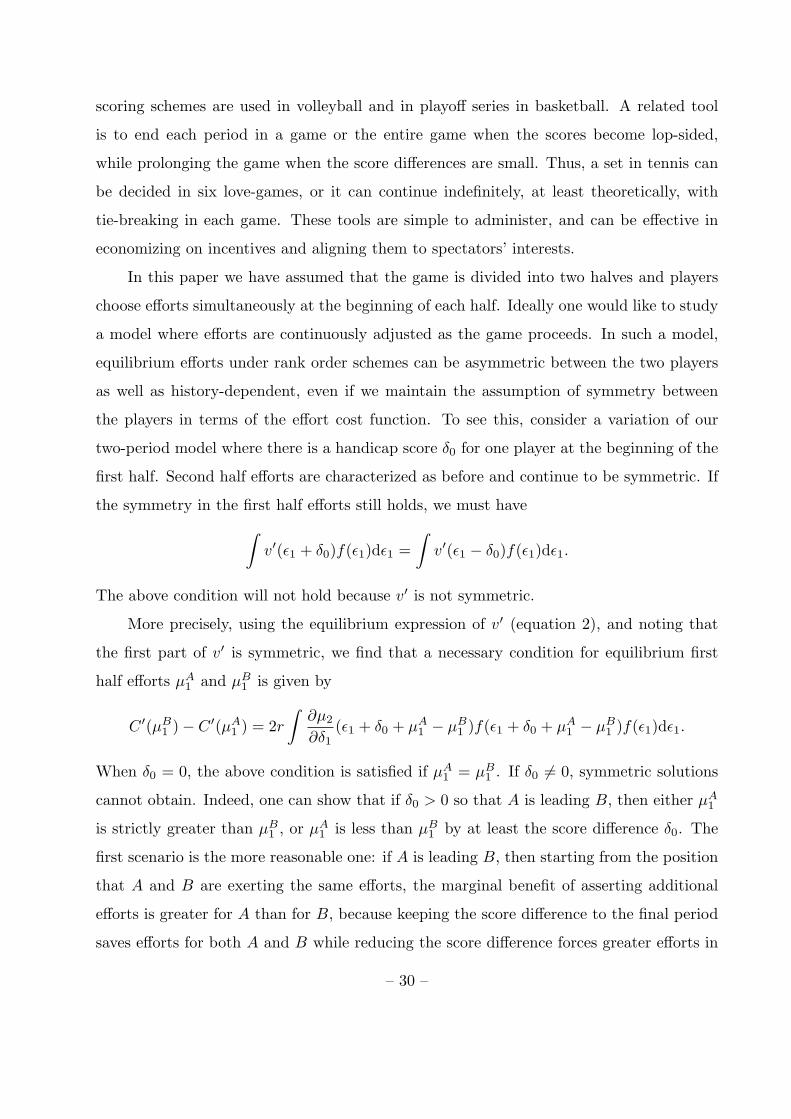
In this paper we have assumed that the game is divided into two halves and players

choose efforts simultaneously at the beginning of each half. Ideally one would like to study

a model where efforts are continuously adjusted as the game proceeds. In such a model,

equilibrium efforts under rank order schemes can be asymmetric between the two players

as well as history-dependent, even if we maintain the assumption of symmetry between

the players in terms of the effort cost function. To see this, consider a variation of our

two-period model where there is a handicap score δ0 for one player at the beginning of the

first half. Second half efforts are characterized as before and continue to be symmetric. If

the symmetry in the first half efforts still holds, we must have∫

v′(ε1 + δ0)f(ε1)dε1 =∫

v′(ε1 − δ0)f(ε1)dε1.

The above condition will not hold because v′ is not symmetric.

More precisely, using the equilibrium expression of v′ (equation 2), and noting that

the first part of v′ is symmetric, we find that a necessary condition for equilibrium first

half efforts µA1 and µB

1 is given by

C ′(µB1 )− C ′(µA

1 ) = 2r

∫∂µ2

∂δ1(ε1 + δ0 + µA

1 − µB1 )f(ε1 + δ0 + µA

1 − µB1 )f(ε1)dε1.

When δ0 = 0, the above condition is satisfied if µA1 = µB

1 . If δ0 6= 0, symmetric solutions

cannot obtain. Indeed, one can show that if δ0 > 0 so that A is leading B, then either µA1

is strictly greater than µB1 , or µA

1 is less than µB1 by at least the score difference δ0. The

first scenario is the more reasonable one: if A is leading B, then starting from the position

that A and B are exerting the same efforts, the marginal benefit of asserting additional

efforts is greater for A than for B, because keeping the score difference to the final period

saves efforts for both A and B while reducing the score difference forces greater efforts in

– 30 –

the final period from both players. This scenario is consistent with Dixit’s (1987) result

that in a static tournament the favored player has incentives to over-commit efforts in

order to preempt his opponent. But stronger conditions on the density function f and

the cost function C are needed to exclude the other possibility of µA < µB − δ0, and to

characterize the effort dynamics. Nevertheless, this does not invalidate the conclusion that

spectators’ demand for suspense is a necessary ingredient in explaining why the rank order

tournament is the dominant form of rewarding scheme in sports competitions.

6. Conclusion

This paper answers a fundamental question in the economics of sports: why are rank

order schemes the dominant form of incentive mechanism used in sports? Our answer is

that spectators of a sporting event care about efforts of contestants when there is suspense

about the outcome, not about the efforts per se. This conclusion is reached by considering a

dynamic version of tournaments first studied by Lazear and Rosen (1981). When spectators

care only about efforts in the game, we find that linear score difference schemes dominate

rank order schemes, in the sense that the former induces greater effort with lower expected

reward. But when we incorporate the preference for suspense, which type of scheme

is better depends on how much spectators demand suspense. The more spectators enjoy

suspense, the better rank order schemes perform relative to linear score difference schemes.

When spectators’ demand for suspense is sufficiently high, the optimal rank order scheme

not only dominates linear score difference schemes, but can also outperform a broad class

of schemes based on the final score difference.

The theory of contract has made much progress since the 1970s. Optimal design

of incentive schemes has become a standard exercise, and applications of the theory have

found success in many fields, including labor economics, industrial organization, and sports

(Prendergast, 1999). However, empirical validation of the theory has lagged behind.17 In

17 Prendergast (1999) identifies this problem as he concludes his survey: “The typical theoreticalpaper addresses how a certain institution may be optimal. Comparative statics, when offered, are usuallyof the form that institutions or contracts are likely to vary with certain parameters. However, almost notheoretical work has distinguished among plausible theories there.” Chiappori and Salanie (2003) echothe same sentiment at the start of their survey of recent empirical works based on the contract theory:“Many papers consist of theoretical analyses only. Others state so-called stylized facts often based fragileanecdotal evidence and go on to study a model from which these stylized facts can be derived.”

– 31 –

the present paper we take the theory of contract to task and contrast the theory with

observed practices in incentive design. Our purpose is not to construct another theoretical

model based on some assumptions about the contractual environment and use the model

to derive optimal incentive design. Instead, we argue that by contrasting what contract

theory predicts with the incentive schemes that are used in practice, we can learn much

about the contractual environment. Our fundamental assumption is that incentive schemes

that are used in practice should outperform those that are not.

We apply this methodology of “reverse engineering” to sports, where incentives are

an important motivating factor for participating agents, and observations about actual

incentive designs are indisputable. We show that the observation that rank order incentive

schemes are preferred to linear incentive schemes implies that spectators do not care only

about contestants’ effort. We identify a class of consumer preferences which incorporates

the demand for suspense, and under which rank order schemes can dominate linear schemes.

This class of consumer preferences is consistent with what can be directly estimated from

revealed preferences in the empirical sports literature. By identifying consumer tastes from

observed incentive design, this work also contributes to the recent literature that explores

the structure of consumer preferences (Becker, 1996).

An important assumption in our model of dynamic sports competitions is that con-

testants have the same abilities. This is a simplification made to facilitate characterization

of the equilibrium under rank order schemes. Incorporating heterogeneity among contes-

tants removes symmetry in equilibrium and complicates the analysis, but it can also bring

potentially important insights. Incentive schemes that recognize differential abilities, such

as handicapping, have been discussed by Lazear and Rosen (1981) in the context of the

optimal rank order scheme, and extended more recently by Moldovanu and Sela (2001) to

situations where abilities are private information. It would be interesting to explore these

implications in a dynamic context, particularly since our model offers a general framework

for comparing rank order schemes and schemes based on other relative performance mea-

sures. Quite apart from its function as an incentive device, rank order tournament may also

serve a sorting function when contestants are heterogeneous and information is imperfect.

Indeed, it may be argued that in actual competitions, identifying the athletes with supe-

rior abilities is as important as rewarding those who exert great efforts. This is also true

– 32 –

in promotion tournaments in internal labor markets, where efficiency often dictates the

identification and assignment of superior talents to more senior positions in the hierarchy,

as well as in patent races, where fixed financial benefits are awarded based on rank order

comparisons of the proposed designs, even though the social value of a patented design

depends on how “innovative” it is relative to other designs. In these cases, the mechanism

designer is faced with the challenge of structuring the contest to efficiently differentiate

the contestants. When effort is costly and the value of continuing effort depends on the

state of the competition as well as on the abilities of the contestants, a model of dynamic

competition that incorporates both sorting of abilities and incentives for efforts may offer

insights that are otherwise lost in a static analysis of the problem.

References

Aron, D.J., Lazear, E.P., 1990. The introduction of new products. American EconomicReview 80, 421-426.

Becker, G.S., 1996. Accounting for Tastes. Harvard University Press, Cambridge andLondon.

Brocas, I., Carrillo, J., 2002. Do the “three-point victory’ and “golden goal” rules makesoccer more exciting? A theoretical analysis of a simple game. Forthcoming Journal ofSports Economics.

Cabral, L.M., 2003. R&D competition when firms choose variance. Journal of Economicsand Management Strategy 12, 139-150.

Chiappori, P., Salanie, B., 2003. Testing contract theory: A survey of some recent work,In: M. Dewatripont, L.P. Hansen and S.J. Turnovsky (Eds.), Advances in Economics andEconometrics, Vol. 1. Cambridge University Press, London.

Dixit, A., 1987. Strategic behavior in contests. American Economic Review 77, 891-898.

Ehrenberg, R.G., Bognanno, M.L., 1990. Do tournaments have incentive effects? Journalof Political Economy 98, 1307-1324.

Fernie, S., Metcalf, D., 1990. It’s not what you pay it’s the way that you pay it and that’swhat gets results: Jockeys pay and performance. Labour 13, 704-789.

Fort, R., Quirk, J., 1995. Cross-subsidization, incentives, and outcomes in professionalteam sports leagues. Journal of Economic Literature 33, 1265-1299.

Harris, C., Vickers, J., 1987. Racing with uncertainty. Review of Economic Studies 54,1-21.

– 33 –

Holmstrom, B., 1982. Moral hazard in teams. Bell Journal of Economics 13, 324-340.

Holmstrom, B., Milgrom, P., 1987. Aggregation and linearity in the provision of intertem-poral incentives. Econometrica 55, 303-328.

Knowles, G., Sherony, K., Haupert, M., 1992. The demand for major league baseball: Atest of the uncertainty of outcome hypothesis. American Economist 36, 72-80.

Lazear, E.P., Rosen, S., 1981. Rank order Tournaments as Optimum Labor Contracts.Journal of Political Economy 89, 841-864.

Mirrlees, J., 1974. Notes on welfare economics, information and uncertainty, In: M. Balch,D. McFadden, and S. Wu, (Eds.), Essays in Economic Behavior under Uncertainty, pp.243-258.

Moldovanu, B., Sela, A., 2001. The optimal allocation of prizes in contests. AmericanEconomic Review 91, 542-558.

O’Keeffe, M., Viscusi, W.K., Zeckhauser, R.J., 1984. Economic contests: Comparativereward schemes. Journal of Labor Economics 2, 27-56.

Palomino, F., Rigotti, L., 2000. The sport league’s dilemma: Competitive balance andincentives to win. Woking paper, Tilburg University.

Palomino, F., Rigotti, L., Rustichini, A., 2000. Skill, strategy, and passion: An empiricalanalysis of soccer. Working paper, Tilburg University.

Prendergast, C., 1999. The provision of incentives in firms. Journal of Economic Literature37, 7-63.

Sanderson, A., 2002. The many dimensions of competitive balance. Journal of SportsEconomics 3, 204-228.

Szymanski, S., Kesenne S., 2004. Competitive balance and gate revenue sharing in teamsports. Journal of Industrial Economics 52, 165-177.

– 34 –