Survivorship Bias and Mutual Fund Performance:

Relevance, Significance, and Methodical Differences

Abstract

This paper is the first to systematically test the significance of survivorship bias using a

comprehensive database and to test the significance of the differences of survivorship biases

resulting from different methodical approaches. We apply the various methods most

commonly used in the literature on a uniform dataset. In addition, we analyze the performance

of closed funds as the driver of survivorship bias and the performance of new funds as the

driver of incubation bias. Our main findings are: i) Ignoring closed funds leads to a

significantly positive survivorship bias. This is in line with previous research. ii) The choice

of methods leads to statistically and economically significant differences in survivorship bias

estimates. We are able to suggest a bias-minimizing combination of methods if survivorship

bias-free data is not available. iii) The performance of closed funds drives survivorship bias

since these funds underperform surviving funds years before they are closed. iv) We find

evidence for incubation bias in our data but its impact is rather small and clearly depends on

the methods applied.

Keywords: Mutual Fund Performance, Survivorship Bias

JEL Classification: G 11, G 12

4

1 Introduction

Survivorship bias affects almost every empirical study of financial data. Apart form

studies in mutual fund performance where the existence of survivorship bias is well

documented the problem also arises with respect to other financial instruments such as

stocks (e.g., Brown/Goetzmann/Ross, 1995, Boynton/Oppenheimer, 2006) or hedge

funds (e.g., Brown/Goetzmann/Ibbotson, 1999, Liang, 2000, Amin/Kat, 2003).

Unfortunatelly not all researchers assessing mutual fund performance have access to

survivorship bias-free databases like CRSP. Many commercial datasets still include

only funds currently in operation and available for investment. Not accounting for

closed funds can produce inaccurate results especially in studies analyzing the

performance of fund portfolios like the entire fund market. In general, survivorship bias

leads to overestimating the performance of a fund portfolio as the predominant reason

for closing funds is inferior performance (e.g., Malkiel, 1995, Brown/Goetzmann, 1995,

Elton/Gruber/Blake, 1996). For example, the unbiased Jensen alpha of the US domestic

equity mutual fund market was -95 basis points per year in the period from 1993

through 2006. The respective biased result was +14 basis points per year. To avoid

biased results like this in empirical analyses of fund portfolios, it is therefore important

to account for survivorship bias. Consequently, a considerable number of articles

address this issue either as main subject or as additional information by estimating the

amount of (potential) survivorship bias in the datasets analyzed. Noticeably, there is no

study testing the significance of survivorship bias on comprehensive real return data.1

1 Grinblatt and Titman (1989) construct “hypothical returns” on basis of quarterly fund holdings of a very limited set of funds which they use to test significance of survivorship bias. The construction of their dataset suggests that the sample itself is not free of survivorship bias. Malkiel (1995) as well as Deaves (2004) test the performance difference of closed and surviving funds, which in our understanding is not the commonly used definition of survivorship bias.

5

Moreover, survivorship bias estimates reported by these studies vary from 1 to 271

basis points per year (e.g., Grinblatt/Titman, 1989, Deaves, 2004). Apart from

differences in the datasets most studies also show different methods making it difficult

to compare results or decide on the proper size of survivorship bias. Our contribution to

the survivorship bias literature is the first study systematically testing the significance of

survivorship bias as well as analyzing and testing the differences of survivorship bias

estimates resulting from different methodical approaches based on a comprehensive

dataset.

The main methodical differences are in respect to the definition of surviving funds

and to the weighting schemes used for aggregating portfolio returns. The first

predominant definition of surviving funds is commonly known as end-of-sample

conditioning where all funds operating at the end of a specific sample period are defined

as survivors (e.g., Carhart et al., 2002). This approach is followed by, e.g., Wermers

(1997), ter Horst/Nijman/Verbeek (2001), Carhart et al. (2002), Otten/Bams (2004), and

Deaves (2004). The second common survivor definition defines only funds as survivors

that were operational throughout the whole sample period, henceforth named full-data

survivors. Obviously, these funds are a subset of the end-of-sample survivors. The full-

data definition is used in studies by, e.g., Grinblatt/Titman (1989), Brown/Goetzmann

(1995), Elton/Gruber/Blake (1996) and Holmes/Faff (2004). Malkiel (1995) uses both

definitions.2 Another important difference in determining survivorship bias is the

weighting scheme used for aggregating fund portfolio returns. The two schemes

commonly applied in the literature are equal-weighting and value-weighting of

2 Carhart et al. (2002) identify look-ahead conditioning as another type of survivor definition. To our best knowledge look-ahead bias plays a more important role in analyses of performance persistence as it requires funds to survive for two subsequent time periods. In a sense look-ahead survivorship is a two period extension of full-data survivorship.

6

individual fund returns by their total net assets. Despite many studies showing closed

funds to be smaller than surviving funds (e.g., Carhart, 1997, Zhao, 2005), most studies

use equally-weighted portfolio returns as basis for determining fund portfolio

performance and survivorship bias. Studies using value-weighted portfolio returns are,

e.g., Brown/Goetzmann (1995), Malkiel (1995), and Deaves (2004).

There are no two studies sharing an identical set of definitions and methods to

determine survivorship bias. Therefore, there is a need to analyze the impact of different

approaches on the respective survivorship bias estimates. Our analysis fills this gap by

systematically computing and testing survivorship bias with different combinations of

survivor definitions and weighting schemes based on a uniform fund sample. We show

the methodical approach applied to be crucial for survivorship bias estimates and that

the resulting differences of survivorship biases are significant. In addition, we analyze

in detail the performance of closed funds as the main driver of survivorship bias. We

highlight closed funds showing significantly inferior performance and a loss of total net

assets years before they are actually closed. Moreover, we analyze the performance of

new funds as the main driver of incubation bias, which the database we use is

commonly assumed to suffer from (e.g., Arteaga, 1998, Deaves, 2004, Evans, 2007).

We find evidence for incubation in our data, but it is rather small compared to the

underperformance of closed funds. Especially when value-weighted the results are not

significant.

The remainder of this article is organized as follows. Section 2 presents the methods

we use in our analysis. We describe our fund sample and report summary statistics in

Section 3. Section 4 presents empirical results and interpretations. Section 5 concludes.

7

2 Methodology

We define survivorship bias as the performance difference of two fund portfolios, an

unbiased and a biased one. The unbiased portfolio consists of all relevant funds that

were operational at any time during the sample period. Although an investor cannot

actually invest in this portfolio this definition is most appropriate for evaluating the true

historical performance of the fund portfolio or of the aggregate management of these

funds, respectively. The biased portfolio is a subset of the unbiased portfolio including

only funds defined as survivors. It is possible to invest in this portfolio. However, the

historical performance of the biased portfolio draws a wrong picture.

In contrast to our definition of the unbiased portfolio, a portfolio that does not allow

for newly opened funds to enter is not unbiased (“follow the sample” approach, e.g.,

Grinblatt/Titman, 1989, and Elton/Gruber/Blake, 1996). Also, the performance

difference of survivors and closed funds examined as survivorship bias by Deaves

(2004) does not match our definition, as it does not describe the original distortion

caused by ignoring closed funds in a portfolio of funds.

We estimate performance measures based on time series representing the aggregate

monthly returns of a respective fund portfolio. Therefore, we first construct aggregate

fund return time series by monthly averaging (equally- or value-weighted) excess

returns of all funds currently present in the portfolio (e.g., Carhart, 1997, Wermers,

1997, Carhart et al., 2002). This method allows us to use data on all funds regardless of

the length of their return histories. Another advantage of this aggregation method is that

the aggregate time series of all portfolios have the same length and cover the same time

period.

8

Another popular approach is to compute and average performance measures for all

individual funds allocated to the respective portfolio (e.g., Elton/Gruber/Blake, 1996,

Carhart et al., 2002, Deaves, 2004). This has the disadvantage that funds need to have a

return history of a certain length to generate reliable regression estimates (i.e. alphas).

Funds not meeting this criterion, especially funds surviving only for a short period of

time are systematically excluded, which may bias the results. Moreover, since

individual funds partly exist in different time periods their performance measures, in

particular mean excess returns but also Jensen one-factor alphas (Scholz/Schnusenberg,

2008), might show a market climate biased. Due to these disadvantages of the second

approach we only apply the first one of aggregating monthly returns of funds before

determining performance measures for the resulting fund portfolios.3

To show the performance of fund portfolios we follow the majority of studies on

survivorship bias and present results for four different standard performance measures

based on monthly portfolio return time series. (1) The mean excess return µER i with Rit

representing the total return of a fund portfolio i in month t, and Rft representing the risk

free rate of return in month t proxied by the one month US Treasury bill rate.4

µER i = 1

n ∑t=1

T

(Rit − Rft)

(2) The Jensen one-factor-model (Jensen, 1968), with αi representing the selection

performance of the aggregate management of fund portfolio i and Rmt representing the

market index proxied by the value-weighted return of all NYSE, AMEX, and NASDAQ

stocks in month t.

3 Carhart et al. (2002) use both aggregation approaches mentioned above. They report annualized

survivorship bias estimates of 96 bais points and 133 basis points, respectively.

4 http://mba.tuck.dartmouth.edu/pages/faculty/ken.french/Data_Library/f-f_factors.html

9

Rit − Rft = αi + βi (Rmt − Rft) + εit

(3) The Fama-French three-factor-model (Fama/French, 1993), with SMBt capturing

the small firm effect in stock returns proxied by the difference in weighted average

returns on three small cap and three large cap stock portfolios in month t, and with

HMLt capturing the value versus growth effect in stock returns proxied by the difference

in weighted average returns on two value and two growth stock portfolios in month t.

Rit − Rft = αi + β1i (Rmt − Rft) + β2i SMBt + β3i HMLt + εit

(4) The Carhart four-factor-model (Carhart, 1997), with MOMt capturing the

momentum effect in stock returns proxied by the difference in average returns on two

high prior return and two low prior return stock portfolios in month t.5

Rit − Rft = αi + β1i (Rmt − Rft) + β2i SMBt + β3i HMLt + β4i MOMt + εit

To analyze the performance of closed funds as the main driver of survivorship bias

we create aggregate return time series for the closed funds portfolio including only the

returns of a certain runtime before fund closure. This means that these time series only

represent, e.g., last year or second to last year fund returns, etc. These time series are

then compared to the time series of their complement, the end-of-sample survivors, to

evaluate the performance difference of closed and surviving funds (e.g., Deaves, 2004).

To evaluate the performance of new funds as the driver of incubation bias we follow a

similar approach, only that we create time series of different runtimes after fund

opening, e.g. first year or second year fund returns, etc. These are then compared to the

5 http://mba.tuck.dartmouth.edu/pages/faculty/ken.french/Data_Library/det_mom_factor.html

10

time series of their complement, the portfolio of funds existing in the beginning of the

sample period, henceforce starter portfolio.

3 Data

As it is the most complete and accurate dataset on US mutual funds currently

available we use the CRSP Survivor-Bias-Free US Mutual Fund database. Market

factors for our regression analyses are provided by Kenneth R. French via his online

data library.6 Our initial fund dataset contains monthly total returns and total net assets

as well as quarterly fund characteristics on 32,420 US based funds from January 1990

through December 2006. From this dataset we extract our final sample based on the

following selection criteria. First, we exclude all funds not continuously classified as

US domestic equity mutual funds by the Standard & Poors fund objective code.7 As this

classification was first introduced in 1993 we restricted our sample period to January

1993 through December 2006 leaving 11,197 funds in our sample. Then, we eliminate

funds with fragmentary return histories. In addition, funds with identical return histories

(different batches of the same fund) are joined as one fund. Moreover, we exclude funds

with implausible return data (falsely reported or recorded) from the dataset.8 Lastly, we

6 http://mba.tuck.dartmouth.edu/pages/faculty/ken.french/data_library.html

7 The Standard & Poors US domestic equity fund objective codes are Equity USA Aggressive Growth

(AGG), Equity USA Midcap (GMC), Equity USA Growth & Income (GRI), Equity USA Growth (GRO),

Equity USA Income & Growth (ING), Equity USA Small Companies (SCG), and Asset Allocation USA

Preferred (CPF). Average equity holdings (common or preferred stocks) across all funds in our sample

ranges from 78 % (AGG) to 92 % (GMC).

8 Implausible data means monthly returns higher than 50 % or lower than -50 %, respectively. Whenever

possible we checked implausible data through comparison with Morningstar data. Funds were erased if

(1) suspicion was confirmed by Morningstar, or (2) the suspicious data did not fit into the overall return

history of the fund or the respective month.

11

exclude funds without any total net asset data points. Our final sample contains 10,930

US domestic equity mutual funds.

A problem we face with the monthly total net assets is that this data is incomplete for

about one third of the funds in our sample. Therefore, we had to fill missing values in

order to have a complete set of weighting factors. Missing values were filled following

a three step procedure. First, we computed monthly value-weighted average fund

growth rates based on the original data. Then, we filled gaps within time series by

geometric interpolation, assuming constant relative growth between original total net

asset values of individual funds. Third, we extrapolated values missing in the beginning

and at the end of the time series applying the average fund growth rates taken from step

one. In total, we had to fill less than 4.5 % of the monthly total net asset data points or

less than 1.3 % of total net assets, respectively. For less than 3 % of all funds we had to

fill more than 24 months of non-successive missing values. From this we conclude that

the possible impact of filling missing values is, if at all, rather small. As robustness

checks we twice replicated our empirical analysis. First, without estimating any missing

values, and second, with excluding those funds with more than 24 filled months. Apart

from small alterations in the numerical results the economic conclusions and relations

were unchanged.

Furthermore, we observe jumps in some of the total net asset time series that cannot

be explained and therefore could be implausible. 125 funds show total net assets

jumping to more than 10 times their size and back in the following month, or vice versa.

This may be due to reporting or recording errors. Since this has no impact on equally-

weighted results we decided not to exclude these funds from our original analysis. As

12

robustness check we replicated our empirical analysis without these funds. Again,

economic conclusions and relations were unchanged.

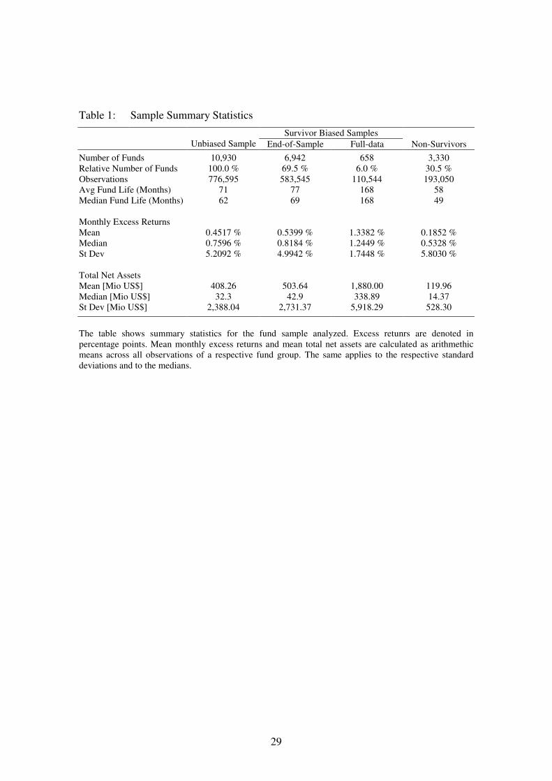
Table 1 shows sample summary statistics. Of the 10,930 funds in our sample 7,600

funds (69.5 %) are end-of-sample survivors, 658 funds (6 %) are full-data survivors,

and 3,330 (30.5 %) funds were closed before December 2006. Therefore, with 30.5 %

of all funds closed there is high potential for survivorship bias. During our sample

period the average (median) fund exists for 71 (62) months, end-of-sample survivors for

77 (69) months, full-data survivors per definition exist throughout the whole 168 (168)

months, and closed funds exist for 58 (49) months. Regarding average (median) returns

of the funds we find distinct differences between the survivor groups. Full-data

survivors show the highest returns with the lowest standard deviation whereas non-

survivors show the lowest returns with the highest standard deviation. Regarding fund

size of the different survivor groups this relation holds as well. Closed funds hold mean

(median) total net assets of 120 (14) million USD when still alive. An average (median)

end-of-sample survivor holds 504 (43) million USD, and full-data survivors hold even

more with 1,880 (339) million USD. Therefore, there is substantial difference between

full-data survivors and survivors without full-data and different weighting schemes.

[Insert Table 1 about here!]

Figure 1 shows the total number of funds and the monthly development of the fund

sample from January 1993 through December 2006. The figure also shows how the

sample divides into the different survivor groups over time. Full-data survivors and

survivors without full-data together make up end-of-sample survivors. The figure shows

13

the US domestic equity mutual fund market substantially growing throughout our

sample period, starting with 1,167 funds in January 1993 and ending with 7,600 funds

operating in December 2006. This clearly shows that constructing an unbiased portfolio

without newly opened funds (Grinblatt/Titman, 1989, and Elton/Gruber/Blake, 1996)

may cause distortion.

[Insert Figure 1 about here]

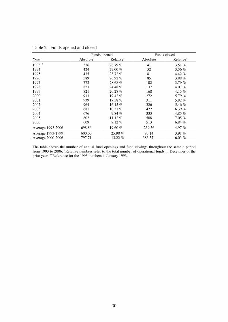
Table 2 reports annual fund openings and fund closings throughout our sample

period. Note that “fund opening” stands for “fund history starts in CRSP”, and “fund

closing” stands for “fund history ends in CRSP” (e.g., Amin/Kat, 2003). In absolute

terms fund openings and closings are accelerating. In relative terms yearly fund

openings almost reduced by half while annual relative fund closings grew from 3.91 %

to 6.03 %, when comparing two seven-year sub-periods. For the period 1962 through

1995 Carhart (1997) reports an even smaller annual fund closing rate of 3.6 %. This

means that for future fund portfolio performance studies survivorship bias becomes an

increasingly important issue if researchers do not have access to bias-free datasets.

[Insert Table 2 about here]

Figure 2 presents the development of the total net assets of different survivor groups

as of December 2006. Although in December 2006 full-data survivors represent only

6 % of the total number of funds they hold just above half (52.5 %) of the fund market’s

total net assets and an even bigger portion throughout our 14-year sample period.

14

[Insert Figure 2 about here]

Obviously, the relationship between fund size and fund performance is an important

issue in the analysis of survivorship bias especially when comparing different weighting

schemes. Some researchers claim that there is a positive relationship between the size of

a fund and its performance due to cost degression and economies of scale. However,

this might be compensated by additional trading cost associated with liquidity

disadvantages as well as price impact if funds grow too large. Indro et al. (1999) find

that fund size in general has a positive impact on fund returns, but quadratic fund size

seems to have a negative impact. From this they conclude that there is an optimal fund

size beyond which size advantages turn into disadvantages. In addition, Chen et al.

(2004) find evidence that the latter relationship holds especially for small cap funds.

When becoming too large these funds have to trade large blocks of potentially illiquid

stocks and thus have a higher impact on stock prices.

Table 3 presents mean total net assets, monthly mean excess returns, and survivor

group membership for decile portfolios of funds sorted by their individual mean total

net assets. The table obviously shows a strong connection of fund size, returns, and full-

data survivorship: the larger a fund the higher the returns. We do not find any evidence

for a negative impact of size on returns. The majority of full-data survivors gather in the

first decile while it contains a relatively small portion of closed funds. Survivors

without full-data are distributed almost evenly across all deciles. Closed funds, although

present in all deciles, have an overbalance in the lower deciles.

[Insert Table 3 about here]

15

The positive relation between fund size and fund returns as well as the fact that full-

data survivors are overrepresented in the higher deciles further encourages the

assumption that the different approaches of weighting individual funds in fund

portfolios yield clearly different survivorship bias estimates for our fund sample.

4 Empirical Results

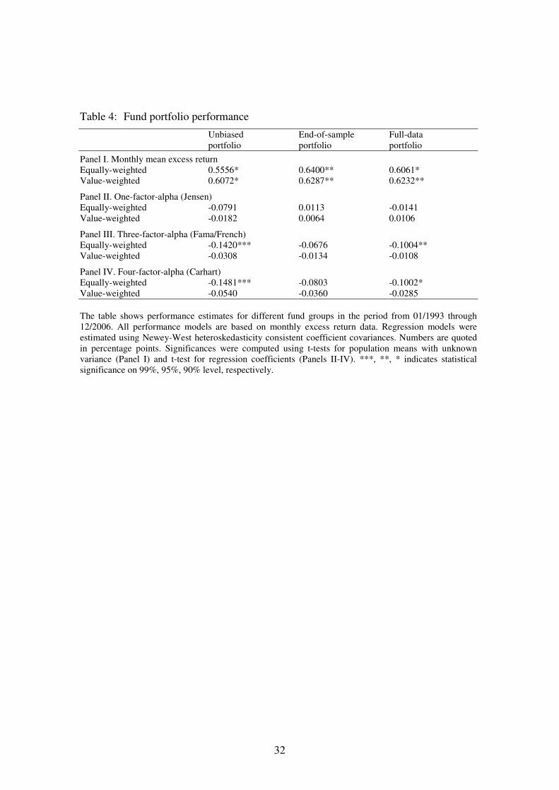
Table 4 reports performance measures for the unbiased as well as for both biased

portfolios. In terms of mean excess returns (Panel I) the end-of-sample survivors show

the highest and most significant results.9 The unbiased results are clearly below the

mean excess returns of both biased portfolios. In terms of risk-adjusted performance

measures (Panels II-IV) a number of conclusions can be drawn from the table. All

unbiased results are lower than the biased results. All unbiased alphas are negative, in

the case of equally-weighted three-factor and four-factor-model highly significant. For

the biased portfolios this is not always the case as the majority of biased Jensen alphas

are positive. This means that besides the performance difference there is also potential

for misinterpreting the average fund manager to have beaten the market during the

sample period. For further conclusions one has to distinguish between different

weighting schemes. In general, value-weighted portfolios show higher (or less negative)

alphas than equally-weighted portfolios. For the unbiased portfolio this relation is most

pronounced as the poor performance of the small non-survivors is overweighted with

equal-weighting. Thus, equally-weighted portfolios are more susceptible to survivorship

bias than value-weighted portfolios. In the case of equal-weighting the end-of-sample

9 Significances for single measures are tested using (two-sided) t-tests for population means with

unknown variances (mean excess returns) and (two-sided) t-tests for regression coefficients (alphas).

Regression models were estimated using Newey-West heteroskedasticity consistent coefficient

covariances.

16

portfolio always shows the highest alphas. This means that equally-weighted end-of-

sample portfolios are more susceptible to survivorship bias than full-data portfolios.

Value-weighted the full-data alphas are highest and therefore most susceptible to

survivorship bias

[Insert Table 4 about here.]

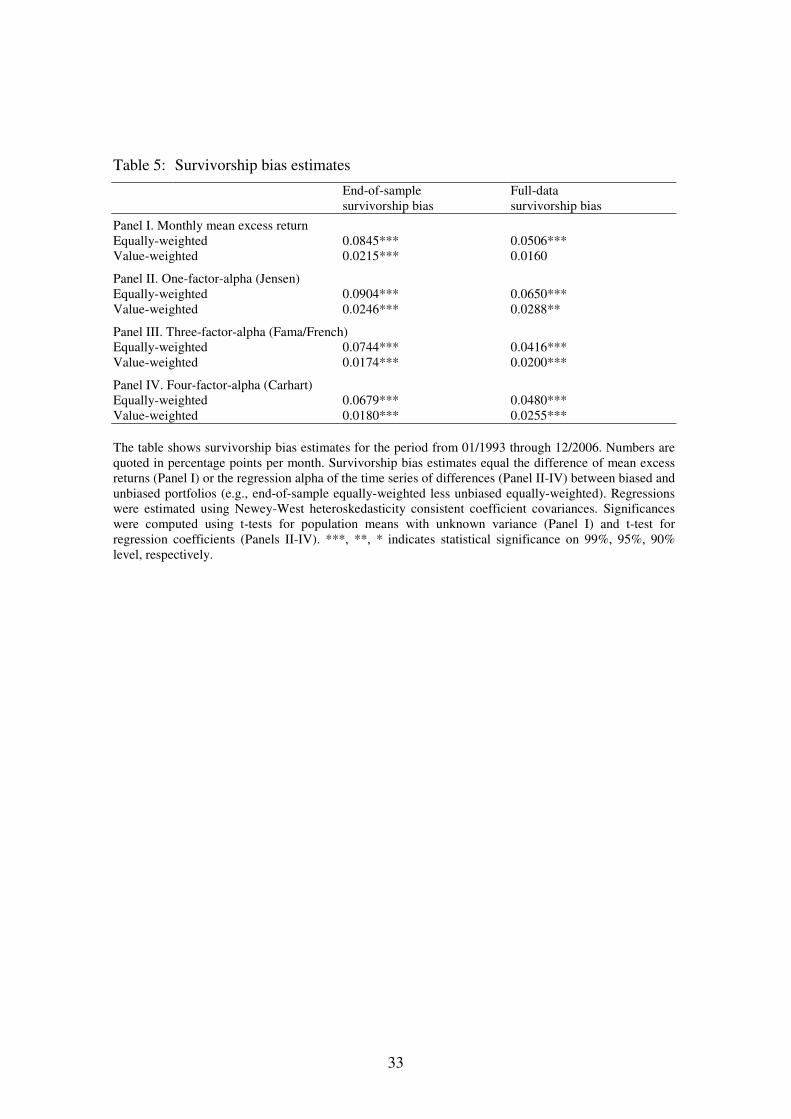
Table 5 reports survivorship bias estimates. Across all performance measures and

method combinations survivorship biases are positive and, with just one exception,

highly statistically significant.10 This confirms previous research reporting that

survivorship bias in general overstates fund portfolio performance. Statistically

significant results range from 1.74 to 9.04 basis points per month, or 21 to 109 basis

points per year, respectively.11 These numbers also confirm previous research, where

the majority of survivorship bias estimates ranged from 20 to 104 basis points per year.

Again, distinguishing different weighting-schemes equal-weighting always yields

higher survivorship bias than value-weighting. With an average of approximatelly 80

basis points per year across all measures and survivor definitions equally-weighted

survivorship bias is both statistically and economically significant. Value-weighted

survivorship bias with an average of approximately 26 basis points per year across

10 Significances for survivorship biases in mean excess returns were tested using (two-sided) t-tests for

two population means (method of paired comparisons) on the time series of differences between biased

and unbiased portfolios (e.g., end-of-sample equally-weighted less unbiased equally-weighted). Since

regression coefficients are additive the difference of alphas equals the alpha of differences. We test

significances for survivorship biases in alphas using (two-sided) t-tests for regression coefficients on the

alpha of the time series of return differences between biased and unbiased portfolios.

11 Annualized by (1 + monthly survivorship bias)12 − 1. Cf. Deaves (2004).

17

measures and survivor definitions on the other hand seems economically of minor

importance. Concerning the performance measure applied the one-factor-alpha seems to

be most susceptible to survivorship bias as it shows the highest results. The Fama-

French three-factor-alpha seems to be the least susceptible to survivorship bias.

Concerning method combinations the equally-weighted end-of-sample survivorship

biases are the highest with an average of 95 basis points per year across all measures.

The value-weighted end-of-sample estimates are the lowest with an average of 25 basis

points per year across all measures.

[Insert Table 5 about here]

Table 6 analyzes and tests the differences from the four method combinations by

reporting differences of full-data and end-of-sample survivorship biases (Panel I) as

well as differences of value-weighted and equally-weighted results (Panel II). Panel I

shows that the end-of-sample survivorship bias is larger than the full-data survivorship

bias for equal weighting with statistical significance for mean excess returns, three-

factor-alphas, and four-factor-alphas.12 However, the differences are rather small and

seem economically of minor importance. A possible explanation could be drawn from

the role of small funds. Underperforming small funds are either closed or carried

12 Significances for differences in survivorship biases in means excess returns where tested using (two-

sided) t-tests for two sample means (method of paired comparisons), the differences in survivorship

biases in alphas were tested using (two-sided) t-tests for regression coefficients on the alphas of times

series of differences. In Panel I of Table 5 these time series were constructed as differences of biased

portfolios (e.g. end-of-sample equally-weighted less full-data equally-weighted). In Panel II of Table 5

these time series were constructed as differences of performance differences of biased and unbiased

portfolios (e.g. (end-of-sample equally-weighted less unbiased equally-weighted) less (end-of-sample

value-weighted less unbiased value-weighted)).

18

through maybe due to long histories and popularity reasons. Supporting evidence is

given in Table 3 where full-data funds can be found across all TNA-deciles, except for

the lowest. This means that equally-weighted small funds disproportionally decrease the

performance of the full-data portfolio. On the other hand outperforming small funds

disproportionally increase the equally-weighted performance of the end-of-sample

portfolio, possibly due to incubation. As a result the equally-weighted end-of-sample

survivorship bias should be higher than full-data survivorship bias. Further supporting

evidence is given in Table 4 showing end-of-sample survivors always outperforming

full-data survivors in the case of equally-weighting.

[Insert Table 6 about here]

With value-weighting full-data survivorship bias results are on average slightly

higher than end-of-sample results, though without statistical or economical significance.

This is because through value-weighting the disproportional impact of small funds does

not occur, as described in the previous paragraph. Since the relative proportion of large

funds with superior performance is noticeably higher in the full-data portfolio value-

weighting has more impact on the full-data portfolio. Table 4 supports this assumption

by showing difference in performance from equally-weighting to value-weighting being

always higher when using the full-data definition.

Panel II in Table 6 shows more distinct relations as for both survivor definitions

value-weighted survivorship bias results are substantially smaller than equally-weighted

results. This is not surprising as underperforming closed funds have much less impact

on the performance of the unbiased portfolio in the case of value-weighting. All

19

differences are statistically significant regardless of survivor definition and performance

measures. In the case of end-of-sample conditioning the equally-weighted survivorship

biases are on average 71 basis points per year higher than the value-weighted estimates.

This means that equally-weighted survivorship bias is approximately four times higher

than value-weighted, which is economically significant. With full-data the equally-

weighted survivorship biases are on average 35 basis points per year higher than value-

weighted survivorship biases, which is still approximately double the size and therefore

of also economical importance.

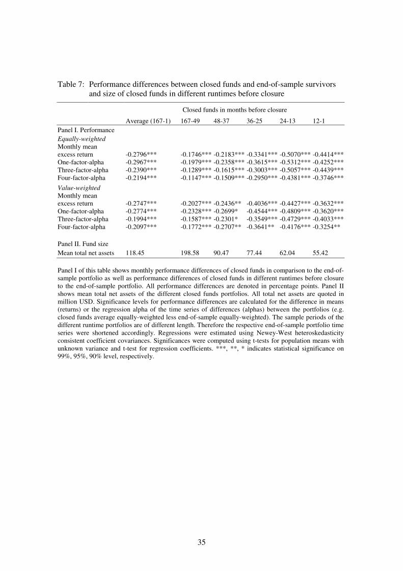
As mentioned before, the inferior performance of closed funds is the driver of

survivorship bias. Total net assets of closed funds are noticeably smaller than those of

surviving funds causing significant differences in results when weighted differently. In

addition to these findings Table 7 reports the performance differences of closed funds

and their complement, the end-of-sample survivors (e.g., Deaves, 2004) and average

total net assets held by closed funds, both average and in different runtimes before fund

closure. To start with the latter, Panel II clearly shows closed funds decreasing in total

net assets about four years before closure. The average performance difference of closed

funds and end-of-sample survivors (Panel I, first column) is highly significant across all

measures and weighting schemes (all p-values < 0.0001). This clearly shows inferior

performance of closed funds being the driver of survivorship bias. The performance

differences range from 20 to 30 basis points per month or 242 to 362 basis points per

year, respectively, which is of high economical importance. These findings confirm

estimates for the Canadian market reported by Deaves (2004) which range from 232 to

271 basis points per year, as well as the 30 basis points per month reported for US

equity funds by Carhart et al. (2002). The remaining columns 2-6 of Panel I show that

20

closed funds underperform end-of-sample survivors regardless of the runtime before

closure. Their performance decreases almost constantly throughout the last 4 years,

except in the last year where performance slightly increases. During their last two years

of existence closed funds underperform surviving funds by more than 400 basis points

per year.

[Insert Table 7 about here]

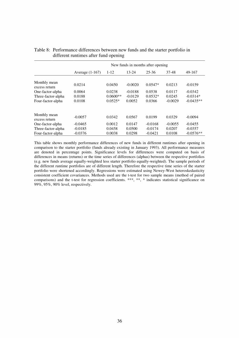
After having examined the performance of closed funds as the driver of survivorship

bias we now analyze the performance of new funds as the driver of incubation bias,

which CRSP is generally suspected to suffer from. Incubation means that fund families

open new funds to the public only after a certain incubation time during which the fund

internally creates a favourable return history. When opened to the public these histories

are backfilled into fund databases. In contrary, funds with inferior performance histories

in the beginning are not opened to the public, and no return histories are reported to

fund databases. Thus, these databases are likely to suffer from incubation bias.

Table 8 reports performance differences between new funds in different runtimes

after opening and their complement, the portfolio of funds existing at the beginning of

the sample period (starter portfolio). The first column shows that new funds on average

slightly outperform the starter portfolio when equally-weighted, but without statistical

or economical significance. There is evidence for outperformance of new funds in the

first and third year of existence by on average 55 basis points per year across all

measures. This confirms our assumption that incubation is responsible for the equally-

weighted end-of-sample survivorship bias being higher than with full-data. However,

21

with value-weighting we find no significant differences between new funds and the

starter portfolio independent of the runtime after opening. Moreover, the first column

shows that on average new funds underperform the starter portfolio. Thus, there seems

to be an incubation bias in our dataset when equally-weighted results are taken into

accout. But its impact is clearly dominated by the underperformance of non-surviving

funds. When value-weighted we find no economically relevant incubation bias in our

data.

[Insert Table 8 about here]

5 Conclusion

Survivorship bias is an important issue in analyses of mutual fund performance as

well as other financial data. Comparing previous studies on mutual funds clearly shows

that there is yet no consistent set of definitions and methods researchers use to estimate

survivorship bias. This makes it difficult to compare results or decide on the proper size

of survivorship bias. We are the first to systematically analyze and test the significance

of survivorship bias and survivorship bias differences from different methods. As main

differences in the methods commonly applied we identified definitions of surviving

funds and weighting schemes for aggregating fund returns. Analyzing the survivorship

bias for US equity mutual fund data we illuminate this problem by applying different

method combinations on a uniform dataset. This allows us to compare the results of

different methods and show their impact on the magnitude of survivorship bias

estimates.

22

In general, we find economically and statistically significantly positive survivorship

bias when ignoring closed funds. In respect to the weighting scheme applied equally-

weighting yields survivorship estimates being twice as high (full-data) or four times as

high (end-of-sample) as when using value-weighting. These differences are both

statistically and economically significant. This is no surprise as closed funds are smaller

while operational than surviving funds. Hence, their influence on the unbiased portfolio

is higher when equally-weighted and smaller when value-weighted. Concerning the

different survivor definitions, the end-of-sample definition shows higher survivorship

bias estimates when equally-weighted than the full-data definition. These results are

statistically significant but economically not as important as the differences in

weighting schemes. The full-data definition yields slightly higher estimates when value-

weighted than the end-of-sample definition, but the results are not significant. As a

result, the choice of methods for analysing mutual fund data is crucial for the magnitude

of survivorship bias experienced when the data is not free of survivorship bias.

Especially the weighting scheme yields economically significant differences.

Analyzing the driver of survivorship bias, we show that closed funds on average

have less total net assets than end-of-sample survivors and underperform end-of-sample

survivors by far regardless of the performance measure used. In addition, we found the

performance and the size of closed funds decreasing in the last four years before fund

closure. In their last two years of existence closed funds underperformed surviving

funds by more than 400 basis points per year.

We also studied the performance of new funds in comparison to the starter portfolio,

which includes only those funds that were existent in the beginning of the sample

period, to evaluate the impact of incubation bias in our dataset. Equally-weighted we

23

find statistically significant evidence, that new funds outperform the starter portfolio by

about 55 basis points per year in their first and third year of existence. However, value-

weighted differences are statistically not significant. This suggests that incubation is of

minor importance with value-weighting. In addition, the underperformance of closed

funds clearly dominates the ourperformance of new funds in terms of magnitude and

significance.

Our results show that survivorship bias exists and that it is economically relevant.

Moreover, the performance of fund portfolios and the survivorship bias following from

ignoring closed funds highly depend on the set of methods applied. Comparing the

different approaches significant results for survivorship bias range from 21 basis points

per year (value-weighted, end-of-sample, three-factor alpha) to economically significant

109 basis points per year (equally-weighted, end-of-sample, one-factor alpha). From

these results we draw several conclusions. First, it is important to use an unbiased

dataset for the measurement of fund portfolio performance. Even more so because fund

closings rates were shown to be increasing while relative fund openings dropped during

our sample period. Second, if an unbiased dataset is not available the Fama-French

three-factor-alpha should be applied on a value-weighted end-of-sample time series as it

yields the least survivorship biased results. Our analysis showed a bias of 21 basis

points per year, which is economically of minor importance. Also, with value-weighting

incubation is of minor importance. Third, to be able to compare the survivorship bias

estimates of new studies to those of previous studies it is important to clearly define the

methods used or maybe even use a common set of definitions and methods to analyze

survivorship bias.

24

References

Amin, G. S., Kat, H. M., 2003. Welcome to the Dark Side: Hedge Fund Attrition and

Survivorship Bias over the Period 1994-2001. Journal of Alternative Investment

Summer 2003, 53−73.

Arteaga, K. G., Ciccotello, C. S., Grant, C. T., 1998. New Equity Funds: Marketing and

Performance. Financial Analyst Journal 54, 43–49.

Boynton, W., Oppenheimer, H., 2006, Anomalies in Stock Market Pricing: Problems in

Return Measurements. Journal of Business 79, 2617–2631.

Brown, S. J., Goetzmann, W. N., 1995. Performance Persistence. Journal of Finance 50,

679−698.

Brown, S. J., Groetzmann, W. N., Ross, S. A., 1995. Survival. Journal of Finance 50,

853–873.

Brown, S. J., Goetzmann, W. N., Ibbotson, R. G., 1999. Offshore Hedge Funds:

Survival and Performance, 1989-95. Journal of Business 72, 91–117.

Carhart, M. M., 1997. On Persistence in Mutual Fund Performance. Journal of Finance

52, 57−82.

Carhart, M. M., Carpenter, J. N., Lynch, A. W., Musto, D. K., 2002. Mutual Fund

Survivorship. Review of Financial Studies 15, 1439−1463.

Chen, J., Hong, H., Huang, M., Kubik, J. D., 2004. Does Fund Size Erode Mutual Fund

Performance? The Role of Liquidity and Organization. American Economic

Review 94, 1276−1302.

CRSP Survivor-Bias-Free US Mutual Fund Database Guide, 2007. Version

CA295.200701.

CRSP Survivor-Bias-Free US Mutual Fund Database Guide, 2008. Version 200803.

Deaves, R., 2004. Data-conditioning biases, performance, persistence and flows: The

case of Canadian equity funds. Journal of Banking and Finance 28, 673−694.

25

Elton, E. J., Gruber, M. J., Blake, C. R., 1996. Survivorship Bias and Mutual Fund

Performance. Review of Financial Studies 9, 1097−1120.

Evans, R. B., 2007. The Incubation Bias. Working Paper, Darden Graduate School of

Business, University of Virginia.

Fama, E. F., French, K. R., 1993. Common risk factors in the returns on stocks and

bonds. Journal of Financial Economics 33, 3−56.

Grinblatt, M., Titman, S., 1989. Mutual Fund Performance: An Analysis of Quarterly

Portfolio Holdings. Journal of Business 62, 393−416.

Holmes, K. A., Faff, R. W., 2004. Stability, Asymmetry and Seasonality of Fund

Performance: An Analysis of Australian Multisector Managed Funds. Journal of

Business Finance & Accounting 31, 539–578.

Indro, D. C., Jiang, C. X., Hu, M. V., Lee, W. Y., 1999. Mutual Fund Performance:

Does Fund Size Matter? Financial Analyst Journal 55, 3, 74−87.

Jensen, M. C., 1968. The Performance of Mutual Funds in the Period 1945-1964.

Journal of Finance 23, 389−416.

Kanji, G. K., 1993. 100 Statistical Tests. Sage Publications, London, Newbury Park,

New Dehli.

Liang, B., 2000. Hedge Funds: The Living and the Dead. Journal of Financial &

Quantitative Analysis 45, 309–326.

Malkiel, B. G., 1995. Returns from Investing in Equity Mutual Funds 1971 to 1991.

Journal of Finance 50, 549−572.

Otten, R., Bams, D., 2004. How to measure mutual fund performance: economic versus

statistical relevance. Journal of Accounting and Finance 44, 203−222.

Scholz, H., Schnusenberg, O., 2008. Ranking of equity mutual funds: The bias in using

survivorship bias-free datasets. Working Paper, Catholic University of Eichstaett-

Ingolstadt and University of North Florida, Ingolstadt and Jacksonville.

26

ter Horst, J. R., Nijman, T. E., Verbeek, M., 2001. Eliminating look-ahead bias in

evaluating persistence in mutual fund performance. Journal of Empirical Finance

8, 345−373.

Wermers, R., 1997. Momentum Investment Strategies of Mutual Funds, Performance

Persistence, and Survivorship Bias. Working Paper, University of Colorado at

Boulder, Boulder.

Zhao, X., 2005. Exit Decisions in the U.S. Mutual Fund Industry. Journal of Business

78, 1365−1401.

27

Figure 1: Fund sample development

0

2,000

4,000

6,000

8,000

10,000

12,000Ja

n 9

3

Jan

94

Jan

95

Jan

96

Jan

97

Jan

98

Jan

99

Jan

00

Jan

01

Jan

02

Jan

03

Jan

04

Jan

05

Jan

06

Month

To

tal

nu

mb

er o

f fu

nd

s

Survivors without full-data

Full-data survivors

Non-survivors

The figure shows the fund sample development in the period from 01/1993 through 12/2006 and how the sample divides into the different survivor groups. Of the total 10,930 funds 3,330 funds (30.5 %) where closed before December 2006 (closed funds), 7600 funds (69.5 %) were in operation in that month (end-of-sample survivors) and 658 of the operational funds (6 % on total) survived throughout the whole sample period (full-data survivors).

28

Figure 2: Total net asset development for the survivor groups as of 12/2006

0

500

1,000

1,500

2,000

2,500

3,000

3,500

4,000Ja

n 9

3

Jan

94

Jan

95

Jan

96

Jan

97

Jan

98

Jan

99

Jan

00

Jan

01

Jan

02

Jan

03

Jan

04

Jan

05

Jan

06

Month

Mar

ket

to

tal

net

ass

ets

[bil

. U

SD

]

Survivors without full-data

Full-data survivors

Non-survivors

The figure shows the development of the markets total net assets for the fund sample split up into different survivor groups as of 12/2006 throughout the period from 01/1993 through 12/2006. In 12/2006 full-data survivors represent 52.5 % of the markets total net assets.

29

Table 1: Sample Summary Statistics

Survivor Biased Samples Unbiased Sample End-of-Sample Full-data Non-Survivors

Number of Funds 10,930 6,942 658 3,330 Relative Number of Funds 100.0 % 69.5 % 6.0 % 30.5 % Observations 776,595 583,545 110,544 193,050 Avg Fund Life (Months) 71 77 168 58 Median Fund Life (Months) 62 69 168 49 Monthly Excess Returns Mean 0.4517 % 0.5399 % 1.3382 % 0.1852 % Median 0.7596 % 0.8184 % 1.2449 % 0.5328 % St Dev 5.2092 % 4.9942 % 1.7448 % 5.8030 % Total Net Assets Mean [Mio US$] 408.26 503.64 1,880.00 119.96 Median [Mio US$] 32.3 42.9 338.89 14.37 St Dev [Mio US$] 2,388.04 2,731.37 5,918.29 528.30

The table shows summary statistics for the fund sample analyzed. Excess retunrs are denoted in percentage points. Mean monthly excess returns and mean total net assets are calculated as arithmethic means across all observations of a respective fund group. The same applies to the respective standard deviations and to the medians.

30

Table 2: Funds opened and closed

Funds opened Funds closed Year Absolute Relative+ Absolute Relative+

1993++ 336 28.79 % 41 3.51 % 1994 424 29.00 % 52 3.56 % 1995 435 23.72 % 81 4.42 % 1996 589 26.92 % 85 3.88 % 1997 772 28.68 % 102 3.79 % 1998 823 24.48 % 137 4.07 % 1999 821 20.28 % 168 4.15 % 2000 913 19.42 % 272 5.79 % 2001 939 17.58 % 311 5.82 % 2002 964 16.15 % 326 5.46 % 2003 681 10.31 % 422 6.39 % 2004 676 9.84 % 333 4.85 % 2005 802 11.12 % 508 7.05 % 2006 609 8.12 % 513 6.84 %

Average 1993-2006 698.86 19.60 % 239.36 4.97 %

Average 1993-1999 600.00 25.98 % 95.14 3.91 % Average 2000-2006 797.71 13.22 % 383.57 6.03 %

The table shows the number of annual fund openings and fund closings throughout the sample period from 1993 to 2006. +Relative numbers refer to the total number of operational funds in December of the prior year. ++Reference for the 1993 numbers is January 1993.

31

Table 3: Size and returns of decile portfolios based on funds sorted by individual mean total net assets

Monthly mean excess returns Decile

Mean total net assets Equally-weighted Value-weighted

Full-data survivors

Survivors without full-

data

Closed funds

1 1,877.60 0.6621 0.6167 56.53 % 8.46 % 4.02 % 2 195.28 0.6414 0.5351 19.45 % 10.44 % 7.21 % 3 83.14 0.6090 0.5320 11.40 % 10.66 % 8.35 % 4 42.07 0.5597 0.5059 6.53 % 10.50 % 9.64 % 5 20.93 0.5095 0.4197 2.43 % 10.40 % 10.66 % 6 10.95 0.4799 0.4021 2.13 % 10.04 % 11.47 % 7 5.27 0.3968 0.3460 0.61 % 9.51 % 12.88 % 8 2.27 0.3424 0.2901 0.76 % 9.32 % 13.24 % 9 0.78 0.2703 0.2192 0.15 % 9.87 % 12.22 % 10 0.12 0.2380 0.2416 0.00 % 10.80 % 10.30 %

100.00 % 100.00 % 100.00 %

The Table shows mean total net assets, monthly mean excess returns, and the proportional allocation of different survivor groups for deciles-of-funds portfolios sorted by individual fund mean total net assets. The first decile represents the largest 10 % of all funds, the tenth decile represents the smallest 10 %. Mean total net assets are quoted in million USD. Monthly mean excess returns are quoted in percentage points. Group membership is quoted in percentage points.

32

Table 4: Fund portfolio performance

Unbiased portfolio

End-of-sample portfolio

Full-data portfolio

Panel I. Monthly mean excess return Equally-weighted 0.5556* 0.6400** 0.6061* Value-weighted 0.6072* 0.6287** 0.6232**

Panel II. One-factor-alpha (Jensen) Equally-weighted -0.0791 0.0113 -0.0141 Value-weighted -0.0182 0.0064 0.0106

Panel III. Three-factor-alpha (Fama/French) Equally-weighted -0.1420*** -0.0676 -0.1004** Value-weighted -0.0308 -0.0134 -0.0108

Panel IV. Four-factor-alpha (Carhart) Equally-weighted -0.1481*** -0.0803 -0.1002* Value-weighted -0.0540 -0.0360 -0.0285

The table shows performance estimates for different fund groups in the period from 01/1993 through 12/2006. All performance models are based on monthly excess return data. Regression models were estimated using Newey-West heteroskedasticity consistent coefficient covariances. Numbers are quoted in percentage points. Significances were computed using t-tests for population means with unknown variance (Panel I) and t-test for regression coefficients (Panels II-IV). ***, **, * indicates statistical significance on 99%, 95%, 90% level, respectively.

33

Table 5: Survivorship bias estimates

End-of-sample survivorship bias

Full-data survivorship bias

Panel I. Monthly mean excess return Equally-weighted 0.0845*** 0.0506*** Value-weighted 0.0215*** 0.0160

Panel II. One-factor-alpha (Jensen) Equally-weighted 0.0904*** 0.0650*** Value-weighted 0.0246*** 0.0288**

Panel III. Three-factor-alpha (Fama/French) Equally-weighted 0.0744*** 0.0416*** Value-weighted 0.0174*** 0.0200***

Panel IV. Four-factor-alpha (Carhart) Equally-weighted 0.0679*** 0.0480*** Value-weighted 0.0180*** 0.0255***

The table shows survivorship bias estimates for the period from 01/1993 through 12/2006. Numbers are quoted in percentage points per month. Survivorship bias estimates equal the difference of mean excess returns (Panel I) or the regression alpha of the time series of differences (Panel II-IV) between biased and unbiased portfolios (e.g., end-of-sample equally-weighted less unbiased equally-weighted). Regressions were estimated using Newey-West heteroskedasticity consistent coefficient covariances. Significances were computed using t-tests for population means with unknown variance (Panel I) and t-test for regression coefficients (Panels II-IV). ***, **, * indicates statistical significance on 99%, 95%, 90% level, respectively.

34

Table 6: Differences of survivorship bias estimates

Panel I. End-of-sample vs. full-data survivorship bias

Equally-weighted Value-weighted Difference Difference

Monthly mean excess returns 0.0339* 0.0055

One-factor-alpha (Jensen) 0.0254 -0.0042 Three-factor-alpha (Fama/French) 0.0328** -0.0026 Four-factor-alpha (Carhart) 0.0199* -0.0075

Panel II. Equally-weighted vs. value-weighted survivorship bias End-of-sample Full-data Difference Difference

Monthly mean excess returns 0.0630*** 0.0346***

One-factor-alpha (Jensen) 0.0658*** 0.0362*** Three-factor-alpha (Fama/French) 0.0570*** 0.0216** Four-factor-alpha (Carhart) 0.0499*** 0.0225**

The table shows differences of the monthly survivorship bias estimates presented by Table 5. All numbers are quoted in percentage points. Significance levels in Panel I refer to the difference in means (returns) or to the regression alpha of time series of differences (alphas) between different biased portfolios [e.g. end-of-sample equally-weighted less full-data equally-weighted]. Significance levels in Panel II refer to the regression alpha of time series of differences between different time series of differences [e.g. (full-data equally-weighted less unbiased equally-weighted) less (full-data value-weighted less unbiased value-weighted)]. Regressions were estimated using Newey-West heteroskedasticity consistent coefficient covariances. Significances were computed using t-tests for population means with unknown variance and t-test for regression coefficients. ***, **, * indicates statistical significance on 99%, 95%, 90% level, respectively.

35

Table 7: Performance differences between closed funds and end-of-sample survivors and size of closed funds in different runtimes before closure

Closed funds in months before closure Average (167-1) 167-49 48-37 36-25 24-13 12-1

Panel I. Performance

Equally-weighted

Monthly mean excess return -0.2796*** -0.1746*** -0.2183*** -0.3341*** -0.5070*** -0.4414*** One-factor-alpha -0.2967*** -0.1979*** -0.2358*** -0.3615*** -0.5312*** -0.4252*** Three-factor-alpha -0.2390*** -0.1289*** -0.1615*** -0.3003*** -0.5057*** -0.4439*** Four-factor-alpha -0.2194*** -0.1147*** -0.1509*** -0.2950*** -0.4381*** -0.3746***

Value-weighted Monthly mean excess return -0.2747*** -0.2027*** -0.2436** -0.4036*** -0.4427*** -0.3632*** One-factor-alpha -0.2774*** -0.2328*** -0.2699* -0.4544*** -0.4809*** -0.3620*** Three-factor-alpha -0.1994*** -0.1587*** -0.2301* -0.3549*** -0.4729*** -0.4033*** Four-factor-alpha -0.2097*** -0.1772*** -0.2707** -0.3641** -0.4176*** -0.3254**

Panel II. Fund size

Mean total net assets 118.45 198.58 90.47 77.44 62.04 55.42

Panel I of this table shows monthly performance differences of closed funds in comparison to the end-of-sample portfolio as well as performance differences of closed funds in different runtimes before closure to the end-of-sample portfolio. All performance differences are denoted in percentage points. Panel II shows mean total net assets of the different closed funds portfolios. All total net assets are quoted in million USD. Significance levels for performance differences are calculated for the difference in means (returns) or the regression alpha of the time series of differences (alphas) between the portfolios (e.g. closed funds average equally-weighted less end-of-sample equally-weighted). The sample periods of the different runtime portfolios are of different length. Therefore the respective end-of-sample portfolio time series were shortened accordingly. Regressions were estimated using Newey-West heteroskedasticity consistent coefficient covariances. Significances were computed using t-tests for population means with unknown variance and t-test for regression coefficients. ***, **, * indicates statistical significance on 99%, 95%, 90% level, respectively.

36

Table 8: Performance differences between new funds and the starter portfolio in different runtimes after fund opening

New funds in months after opening

Average (1-167) 1-12 13-24 25-36 37-48 49-167

Monthly mean excess return

0.0214 0.0450 -0.0020 0.0547* 0.0213 -0.0159

One-factor-alpha 0.0064 0.0238 -0.0188 0.0538 0.0117 -0.0342 Three-factor-alpha 0.0188 0.0600** -0.0129 0.0532* 0.0245 -0.0314* Four-factor-alpha 0.0108 0.0525* 0.0052 0.0366 -0.0029 -0.0435**

Monthly mean excess return

-0.0057 0.0342 0.0567 0.0199 0.0329 -0.0094

One-factor-alpha -0.0465 0.0012 0.0147 -0.0168 -0.0055 -0.0455 Three-factor-alpha -0.0185 0.0458 0.0500 -0.0174 0.0207 -0.0357 Four-factor-alpha -0.0376 0.0038 0.0298 -0.0421 0.0108 -0.0576**

This table shows monthly performance differences of new funds in different runtimes after opening in comparison to the starter portfolio (funds already existing in January 1993). All performance measures are denoted in percentage points. Significance levels for differences were computed on basis of differences in means (returns) or the time series of differences (alphas) between the respective portfolios (e.g. new funds average equally-weighted less starter portfolio equally-weighted). The sample periods of the different runtime portfolios are of different length. Therefore the respective time series of the starter portfolio were shortened accordingly. Regressions were estimated using Newey-West heteroskedasticity consistent coefficient covariances. Methods used are the t-test for two sample means (method of paired comparisons) and the t-test for regression coefficients. ***, **, * indicates statistical significance on 99%, 95%, 90% level, respectively.