Survival Models for the Social and Political Sciences Week 3: … · 2017-02-06 ·...

Survival Models for the Social and Political SciencesWeek 3: The Logic of Survival Models and Single Sample Data

JEFF GILLProfessor of Political Science

Professor of BiostatisticsProfessor of Surgery (Public Health Sciences)

Washington University, St. Louis

Survival Models Class [1]

Introduction

◮ Survival data can be either discrete or continuous depending on how time is measured.

◮ Nonparametric estimators of survival are always discrete, however.

◮ Both books introduce the mathematical underpinnings of survival models in Chapter 2 that were

previewed last week.

◮ The key is understanding the hazard and survival functions.

◮ Next we will move on to Cox regression, which removes distributional assumptions seen this week.


Review of Risk Principles

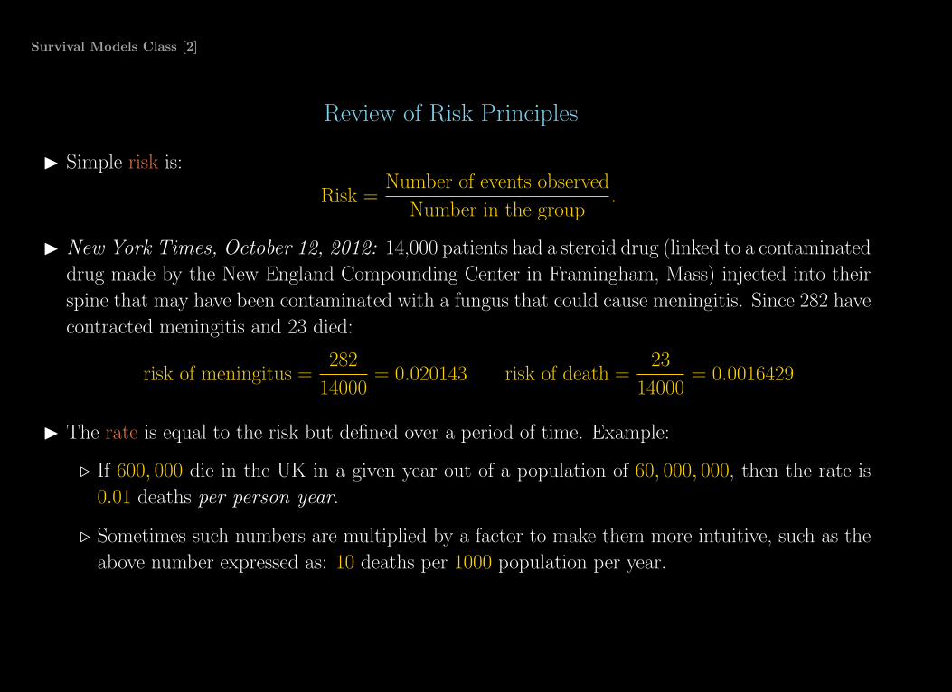
◮ Simple risk is:

Risk =Number of events observed

Number in the group.

◮ New York Times, October 12, 2012: 14,000 patients had a steroid drug (linked to a contaminated

drug made by the New England Compounding Center in Framingham, Mass) injected into their

spine that may have been contaminated with a fungus that could cause meningitis. Since 282 have

contracted meningitis and 23 died:

risk of meningitus =282

14000= 0.020143 risk of death =

23

14000= 0.0016429

◮ The rate is equal to the risk but defined over a period of time. Example:

⊲ If 600, 000 die in the UK in a given year out of a population of 60, 000, 000, then the rate is

0.01 deaths per person year.

⊲ Sometimes such numbers are multiplied by a factor to make them more intuitive, such as the

above number expressed as: 10 deaths per 1000 population per year.



◮ A rate requires the following:

⊲ a specified time period

⊲ a known population size

⊲ the number of events of interest occurring during this period in this population.

◮ Events are divided into types:

⊲ permanent, and the case is considered “no longer at risk” (removed from the at-risk population)

⊲ temporary, and the case eventually returns to the at-risk population.

◮ So temporary exiting cases can return and exit again, raising the rate.



◮ A related quantity to rate that takes into account cases exiting and returning to the at-risk

population is the incidence:

Incidence =Number of events in a defined period

Total person-time at risk× 1000,

also called the incidence density rate and the person-time incidence rate.

◮ Incidence is not Prevalence:

⊲ prevalence is a measure of the total number of cases of disease in a population at any point

in time,

⊲ incidence is the rate of occurrence of new cases over some time period,

. . . so incidence conveys information about the risk of getting the disease, but prevalence indicates

how widespread the disease is and does not cover a time period.



◮ The Crude Mortality Rate (called the “crude death rate”) is:

CMR =Number of deaths occurring in a year

Mid-year population× 1000.

◮ Sometimes “mid-year population” is substituted with “average population”

◮ Multiplying by 1000 is not universal, and 100, 000 is also common.

◮ The Case-Fatality Rate is the proportion of persons with a particular condition (cases) who die

from that condition:

CFR =Number of cause-specific deaths among the incident cases

Number of incident cases× 10n.

◮ Thus CFR is a measure of the severity of the condition.

◮ The time periods for the numerator and the denominator do not need to be the same: the denom-

inator could be cases of HIV/AIDS diagnosed during the calendar year 1990, and the numerator,

deaths among those diagnosed with HIV in 1990, could be from 1990 to the present.



◮ The Age-Specific Mortality Rate is defined as:

ASMR =Number of deaths occurring in a specified age group

Mid-year number in that age group× 1000

◮ The CDC defines specific definitions as well:


Population Attributable Risk

◮ The overall impact of negative effects on public health is a combination of: relative risk and the

proportion of the population exposed.

◮ Denote IPopulation as the incidence in the population, IExposed as the incidence in the exposed group,

and INon-Exposed as the incidence in the unexposed group.

◮ Then the population attributable risk is the excess incidence proportion due to the risk factor:

AR =IPopulation − INon-Exposed

IPopulation=

a+bN (RR − 1)

1 + a+bN (RR − 1)

,

where a+bN is the proportion of the population exposed to the risk factor.

◮ Warning: the epidemiology literature (and others) has other definitions and specialized versions

of the AR.


Population Attributable Risk

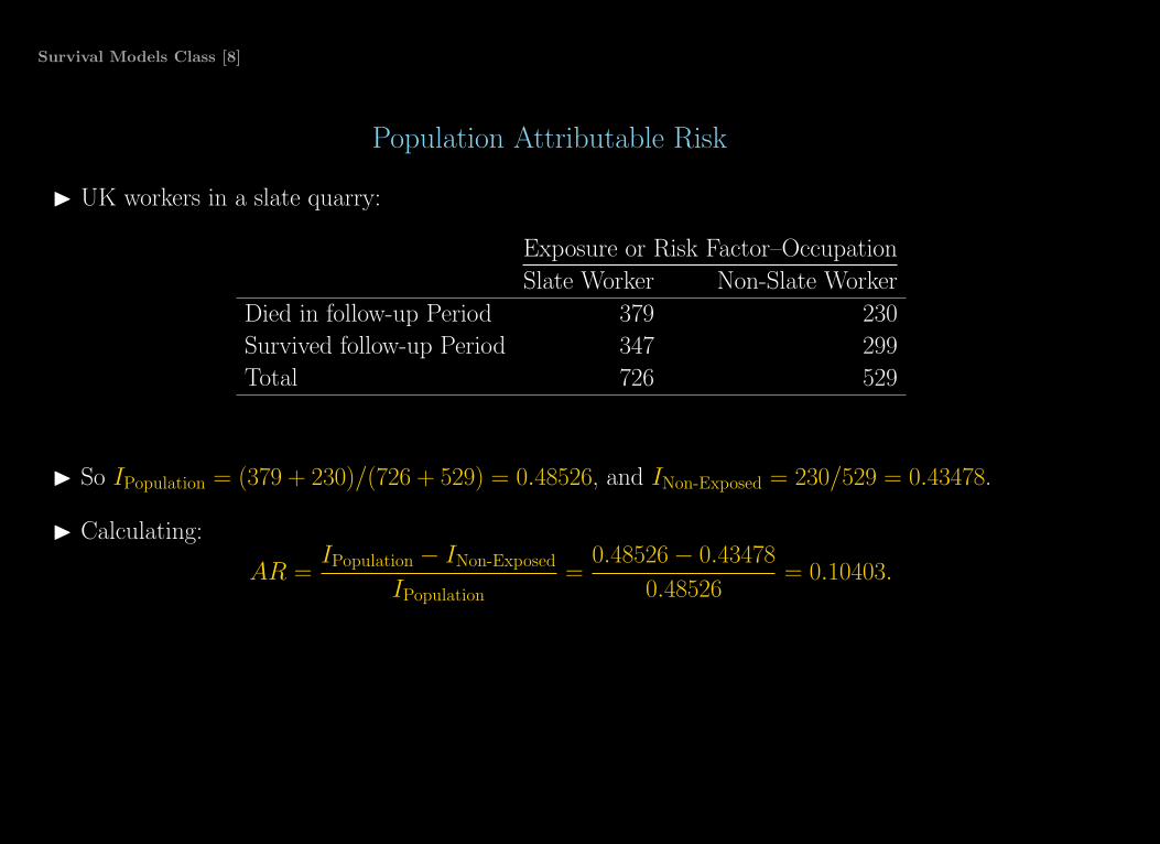
◮ UK workers in a slate quarry:

Exposure or Risk Factor–Occupation

Slate Worker Non-Slate Worker

Died in follow-up Period 379 230

Survived follow-up Period 347 299

Total 726 529

◮ So IPopulation = (379 + 230)/(726 + 529) = 0.48526, and INon-Exposed = 230/529 = 0.43478.

◮ Calculating:

AR =IPopulation − INon-Exposed

IPopulation=

0.48526 − 0.43478

0.48526= 0.10403.


Box-Steffensmeier and Jones Example

Pearson, Frederic S., and Robert A. Baumann. “International Military Intervention, 19461988.

Inter-University Consortium for Political and Social Research, Data Collection 6035.” Ann Arbor, MI

(1993).


Notes on Table 2.1, Right Censoring

◮ The duration of intervention between El Salvador and Honduras is 657 days.

◮ The duration of intervention between Malawi and Mozambique is 631 days.

◮ But these are really very different numbers: Cb = 0 for the first case and Cb = 1 for the second

case.

◮ This means that Malawi-Mozambique is right censored in the data and we do not know when the

intervention ended.

◮ Ignoring this right censoring in the model leads to obviously biased results.


Notes on Table 2.1, Covariate Effects

◮ With survival models what we are really interested in is making standard regression statements

using covariates.

◮ In this case we might be interested in whether contiguity between the two nations affects the

duration of the intervention.

◮ Given such a regression model model (which we are on the way to developing) we will get a

coefficient such that a positive sign means that contiguity elongates the event length and a negative

sign means that contiguity hastens the event.

◮ In the language of survival models we say that contiguity increases or decreases the risk of an

intervention ending.

◮ Contiguity is an example of a time-independent covariate since it is fixed over the length of the

study.

◮ Conversely time-varying covariates (TVCs) are those that can change for cases during the time

covered by the data (in this case say economic variables).


The Heterogeneity of Events

◮ So far we have looked single-spell, single event, or one-way transition processes.

◮ A nation can engage in multiple interventions at the same time.

◮ Events like an intervention can stop and then restart.

◮ An event can occur in multiple ways: an intervention in the example can end because of a treaty,

armistice, third party entrance, surrender, stalemate, compromise, or escalation to a higher order

of militarization.

◮ The Nicaragua-Costa Rica dispute example (BSJ Table 2.2 on page 11) is an example of these

complexities.


The Heterogeneity of Events, Nicaragua-Costa Rica Example

◮ There are multiple spells/duration lengths from multiple MIDs.

◮ There are also multiple events: stalemate and compromise.

◮ Since we know the dates and durations, we also know the duration of peace in between MIDs,

which can also be analyzed with survival models, going from 9 cases to 18.

◮ We learn more by understanding how the event type affects the duration of non-conflict between

MIDs (think about how WWI ended).


Yet Another Swedish Dataset

◮ A life table is constructed for Swedish females in 2010 from Statistics Sweden (SCB) by:

⊲ start with a column for each age: 0-100

⊲ then add a column for the number of females of each age at 2010 (an average of 2010 and 2011

since SCB measures at the end of the year): period data

⊲ the third column is the number of deaths at each age

⊲ risk is deaths/population for each age, for example 117/55407 = 0.0021116

⊲ column 5, alive at age x, is the size of the birth cohort year by year.


Yet Another Swedish Dataset

◮ The last column is the objective of the table:

⊲ it is the size of the birth cohort exposed to previous years of risk

⊲ start with 100, 000 by convention at age 0: synthetic cohort data

⊲ for age 1 we expect 100, 00 × 0.0021 girls to die, leaving 99, 789 at exactly one year of age

⊲ those in the synthetic cohort data live their “lives” under the risk conditions of 2009, as if risk

was locked-in (permanently fixed) at that time.

⊲ this is artificial but useful.


Yet Another Swedish Dataset Life Table


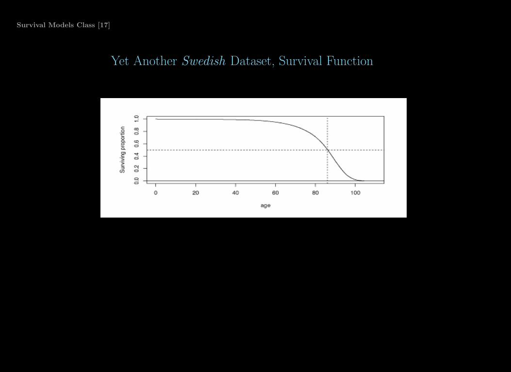
Yet Another Swedish Dataset, Survival Function


Survival Function

◮ The last figure showed the survival function for the SCB data.

◮ This is the probability of surviving past t:

S(t) = p(T ≥ t), t ≥ 0

where T is the random variable for life length, and t is a fixed point of interest.

◮ The Brostrom book alternates between t and t0, and uses the first when making general statements

and the second when talking about a specified time.

◮ In the SCB data T is interpreted as the future life length randomly chosen female from the sample

frame.

◮ In basic models, S(t) is assumed to be smooth and uniformly differentiable at all points.


Theory: Where We Left Off

◮ We will use a proportional hazards model for the critical event.

◮ The hazard function gives the proportion of cases who fail just after time t given that they have

survived until time t.

◮ From a PDF for the event over time, f(t), define the distribution function (CDF) of time t and

the survival function:

F (t) =

∫ t

0

p(T < t)dt S(t) = p(T ≥ t) = 1 − F (t).

The hazard function is created by:

h(t) = limδt→0

[

p(t ≤ T < t + δt|T ≥ t)

δt

]

,

also called the instantaneous hazard rate, the instantaneous death rate, the intensity rate, and

the force of mortality.

◮ Note that:

h(t) =f(t)

S(t)= −

d

dt(log S(t)), S(t) = exp(−H(t)), where H(t) =

∫ t

0

h(u)du


Density Function

◮ The density function is related to the sur-

vival by:

f(t) = −∂

∂tS(t), t ≥ 0.

◮ For a very small s value and arbitrary t0:

p(t0 ≤ T < t0 + s) ≈ sf (t0),

which is illustrated by the figure at right

as an approximation since this is not a

right trapezoid.

◮ More exactly:

f(t) = lims→0

p(t ≤ T < t + s)

s, t ≥ 0,

which is an unconditional statement.


Hazard Function

◮ This is the instantaneous probability of

the event at exactly t, given no event be-

fore then.

◮ Consider the s getting very small, then:

h(t0) = lims→0

p(t0 ≤ T < t0 + s|T ≥ t0)

s,

(for t0 ≥ 0) which is a conditional state-

ment.


The Cumulative Hazard Function

◮ The cumulative hazard function is just the integral of the hazard function (like a CDF):

F (t) = H(t) =

∫ t

0

h(x)dx, t ≥ 0.

◮ Here x is just an integration variable (it goes away), and the Brostrom book confusingly uses s.

◮ This form successively accumulates risk as time continues.

◮ The cumulative hazard function is easier to manipulate in statistical models than the hazard

function, which is a property we will exploit.


Defining Proportional Hazards

◮ Also called “relative risk.”

◮ This is by far the most widely used general survival regression specification.

◮ It starts with a baseline or underlying hazard function that all units share, h(t).

◮ Then the predictors in the form of covariates and associated coefficients act on each units hazard

through exp(Xβ), which is typically called the relative hazard function.

◮ The general form of the regression specification is:

h(t|X) = h(t) exp(Xβ),

◮ An appropriately bounded parametric hazard function can be used for the baseline hazard function.

◮ This week we parametrically define h(t) but next week we will leave it unspecified.


Notes On Proportional Hazards

◮ Depending on the parametric form chosen the relative hazard component may or may not have

an intercept.

◮ The proportional hazards model can be linearized with respect to the RHS by applying the natural

logarithm:

log h(t|X) = log h(t) + Xβ

log H(t|X) = log H(t) + Xβ

◮ Model specifications are exposed to all of the usual concerns about mis-specification.

◮ Additional assumptions Required for the proportional hazards model:

⊲ The true form of the underlying functions, h(t), H(t), and S(t), are all specified correctly.

⊲ The relationship between the linear additive component and the log hazard is linear.

⊲ In the absence of interactions, the linear additive component applies additively on the log

hazard.

⊲ The effect of the linear additive components is the same for all values of time, t.


Proportional Hazards Coefficient Interpretation

◮ Consider how to interpret the jth coefficient from the proportional hazards model.

◮ Recall the elegant interpretation of linear model regression coefficients.

◮ The regression coefficient for Xj (βj) is the increase in the log hazard rate at some fixed point in

t in time if Xj is increased by one unit and all other covariates are held constant:

βj = log(t|X1, X2, ..., [Xj + 1], Xj+1, . . . Xk) − log(t|X1, X2, ..., [Xj], Xj+1, . . . , Xk)

= log

[

t|X1, X2, ..., [Xj + 1], Xj+1, . . . Xk)

t|X1, X2, ..., [Xj], Xj+1, . . . , Xk)

]

◮ This can be re-expressed as:

exp(βj) =

[

t|X1, X2, ..., [Xj + 1], Xj+1, . . . Xk)

t|X1, X2, ..., [Xj], Xj+1, . . . , Xk)

]



◮ Therefore the effect of increasing Xj by 1 is to increase the hazard of the event of study by exp(βj)

at all times (there is no conditionality on time) in:

exp(βj) =

[

t|X1, X2, ..., [Xj + 1], Xj+1, . . . Xk)

t|X1, X2, ..., [Xj], Xj+1, . . . , Xk)

]

◮ Suppose more generally that we increase Xj by some amount δ holding other covariates constant:

∆h(t|X)

log h(t)=

h(t) exp(X′β)

h(t) exp(Xβ)= exp((X′ − X)β)

where X′β is Xβ such that Xj is changed by δ.



◮ Suppose X1 is the treatment indicator: zero for control (X1 = 0), one for treatment (X1 = 1)

with no other explanatory variables.

◮ In this case the proportional hazards model with no intercept is given for the two cases by:

h(t|X1 = 0) = h(t)

h(t|X1 = 1) = h(t) exp(β1)

◮ We can also express the same general effect holding the other explanatory variables constant.


The Exponential Distribution

◮ The simplest model of time to event is the exponential distribution:

f(t) = λe−λt, λ > 0, t ≥ 0,

with expected value 1/λ.

◮ Its hazard function is constant:

h(t) = λ.

◮ The Cumulative hazard function is then:

H(t) =

∫ t

0

h(x)dx = λt,

since:d

dtλt = λ.

◮ The survival function is:

S(t) = e−λt.


The Exponential Distribution

◮ Often the exponential distribution is used to model machine survival.

◮ This has the property called “no aging” since the hazard function stays constant: the hazard rate

plotted against time is a flat line.

◮ The assumption of no aging means that older units have the same hazard as younger units, which

is not very realistic with animal/human survival.

◮ It can be realistic over a short period of time: piece-wise constant hazard.

◮ The percentiles of duration times are given by:

t(p’tile) = λ−1 log

(

100

100 − p’tile

)

where t(p’tile) is the percentile of interest. So the median survival time is calculated by:

t(50) = λ−1 log

(

100

100 − 50

)

= λ−1 log(2).


The Exponential Survival Model

◮ The parametric exponential survival model is specified by linking the single parameter to a linear

additive structure.

◮ So for the ith case the expected duration time is λ−1i = E(ti), leading to:

λ−1i = exp(Xiβ)

where Xiβ includes an intercept.

◮ So that for the full sample:

λ = exp(−Xβ)

meaning that since the hazard rate is h(t) = λ we get:

h(t) = exp(−Xβ)

◮ This can be rewritten as:

h(t) = exp(−β0) exp(−Xβ)

showing that the baseline hazard rate, exp(β0), is a constant here.

◮ Here exp(−Xβ) is called the acceleration factor.



◮ So any change to the hazard rate is purely a function of the linear additive component.

◮ And these changes are then multiplied by the baseline hazard rate.

◮ Suppose we had only one dichotomous explanatory variable in the model:

h(t) = exp(−β0) exp(−x1β1)

meaning that the baseline hazard rate is exp(−β0) applied only for x1 = 0, and the hazard rate

for x1 = 1 is exp(−β0) exp(−x1β1).

◮ This shows the proportional hazards property as simply as possible:

hi(t|x1 = 1)

hi(t|x1 = 0)= exp(−β1)

by notationally equating exp(−β0) = hi(t|x1 = 0), giving the required assumption.



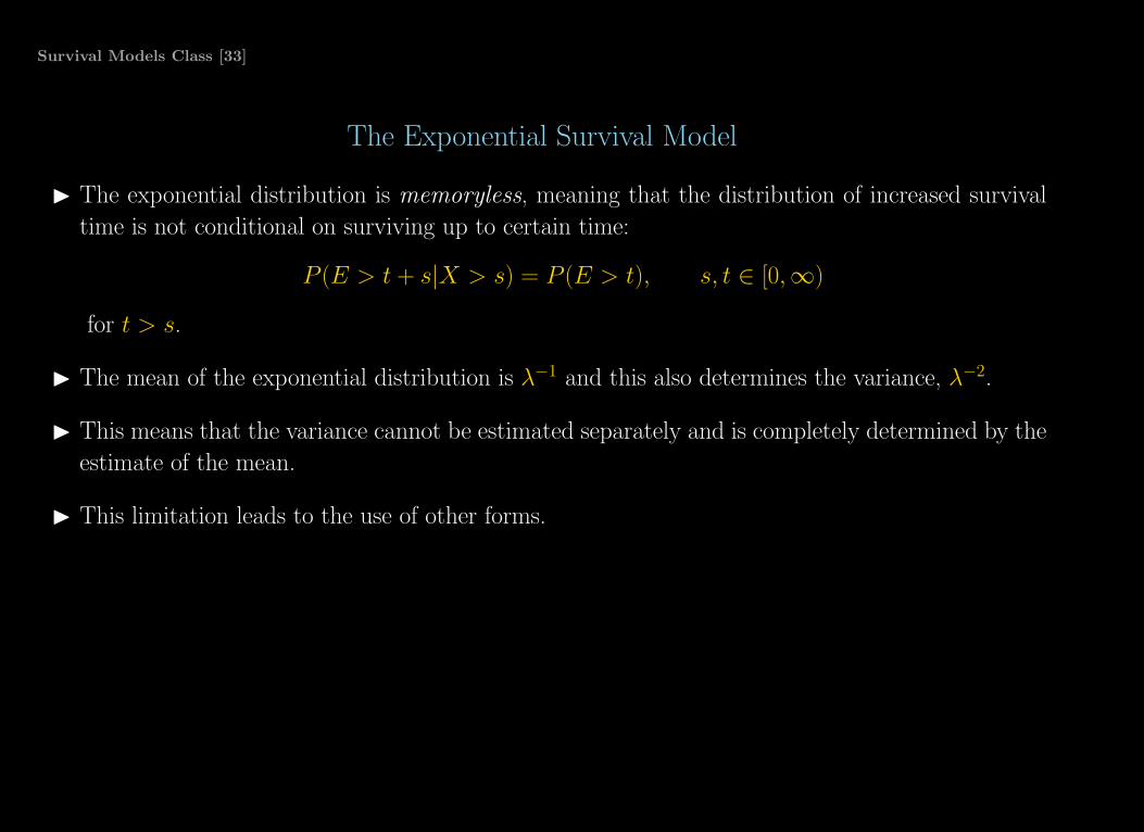
◮ The exponential distribution is memoryless, meaning that the distribution of increased survival

time is not conditional on surviving up to certain time:

P (E > t + s|X > s) = P (E > t), s, t ∈ [0,∞)

for t > s.

◮ The mean of the exponential distribution is λ−1 and this also determines the variance, λ−2.

◮ This means that the variance cannot be estimated separately and is completely determined by the

estimate of the mean.

◮ This limitation leads to the use of other forms.


Exponential Survival Model Illustrated

0 2 4 6 8 10

0.00.2

0.40.6

0.81.0

t

S(t)

0 2 4 6 8 10

0.00.2

0.40.6

0.81.0

t

f(t)

0 2 4 6 8 10

0.00.2

0.40.6

0.81.0

1.2

t

h(t)

λ = 1

λ = 1 2

0.0 0.5 1.0 1.5 2.0 2.5 3.0

01

23

4

t

H(t)


Exponential Survival Model Example

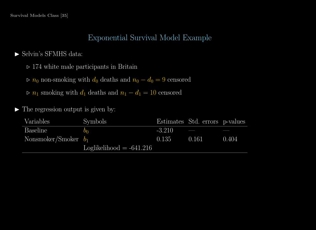
◮ Selvin’s SFMHS data:

⊲ 174 white male participants in Britain

⊲ n0 non-smoking with d0 deaths and n0 − d0 = 9 censored

⊲ n1 smoking with d1 deaths and n1 − d1 = 10 censored

◮ The regression output is given by:

Variables Symbols Estimates Std. errors p-values

Baseline b0 -3.210 — —

Nonsmoker/Smoker b1 0.135 0.161 0.404

Loglikelihood = -641.216


Exponential Survival Model Example

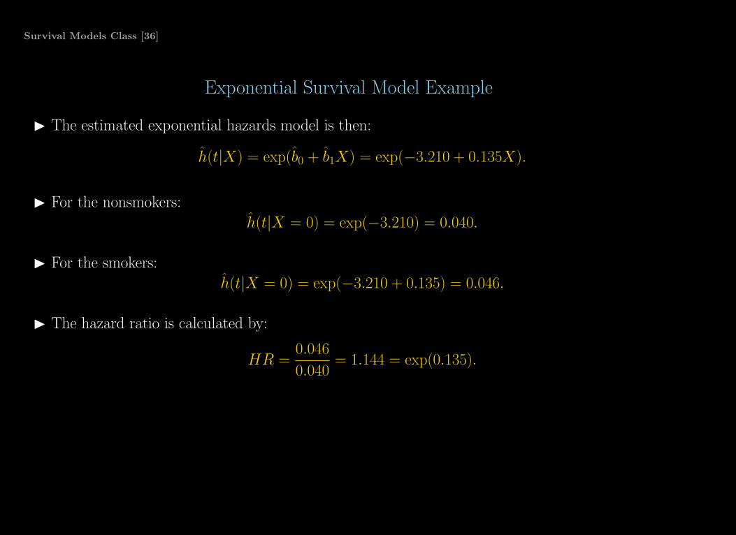
◮ The estimated exponential hazards model is then:

h(t|X) = exp(b0 + b1X) = exp(−3.210 + 0.135X).

◮ For the nonsmokers:

h(t|X = 0) = exp(−3.210) = 0.040.

◮ For the smokers:

h(t|X = 0) = exp(−3.210 + 0.135) = 0.046.

◮ The hazard ratio is calculated by:

HR =0.046

0.040= 1.144 = exp(0.135).


Gamma Distribution

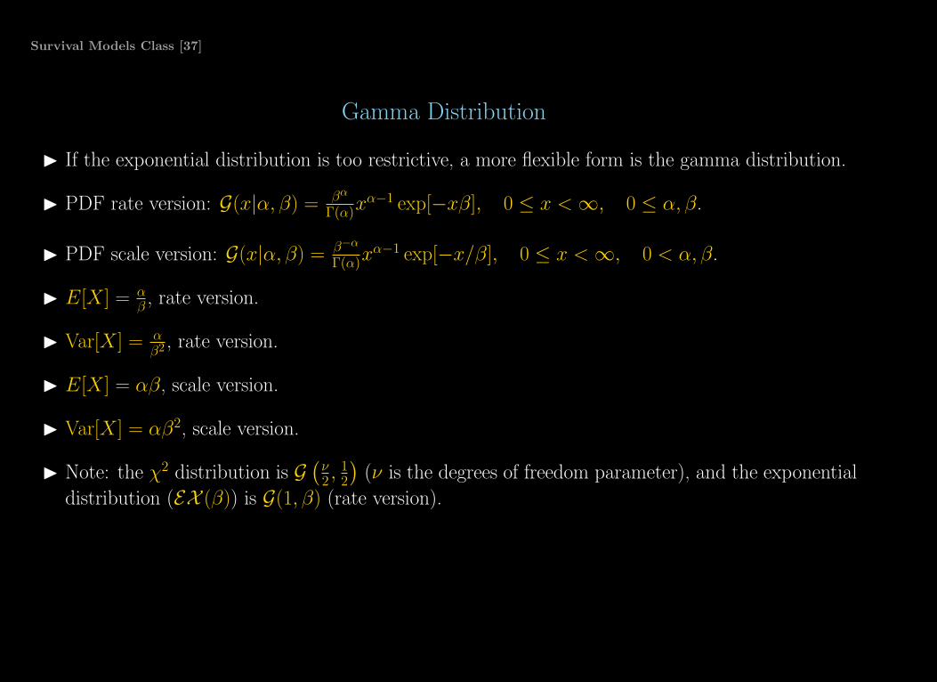
◮ If the exponential distribution is too restrictive, a more flexible form is the gamma distribution.

◮ PDF rate version: G(x|α, β) = βα

Γ(α)xα−1 exp[−xβ], 0 ≤ x < ∞, 0 ≤ α, β.

◮ PDF scale version: G(x|α, β) = β−α

Γ(α)xα−1 exp[−x/β], 0 ≤ x < ∞, 0 < α, β.

◮ E[X ] = αβ , rate version.

◮ Var[X ] = αβ2 , rate version.

◮ E[X ] = αβ, scale version.

◮ Var[X ] = αβ2, scale version.

◮ Note: the χ2 distribution is G(

ν2 ,

12

)

(ν is the degrees of freedom parameter), and the exponential

distribution (EX (β)) is G(1, β) (rate version).


Gamma Survival Model

◮ Express the gamma survival model PDF in the rate version with survival notation:

f(t) =λρ

Γ(ρ)tρ−1 exp[−tλ]

where 0 ≤ t < ∞, λ, ρ > 0.

◮ The survival function can on be expressed with an integral:

S(t) = 1 −1

Γ(ρ)

∫ λt

0

xρ−1 exp(−x)dx.

◮ We then have the hazard function by:

h(t) =f(t)

S(t)

which increases monotonically if ρ > 1, decreases monotonically if ρ < 1, and tends to λ as t

goes to infinity.

◮ When ρ = 1, the gamma model simplifies to the exponential model.


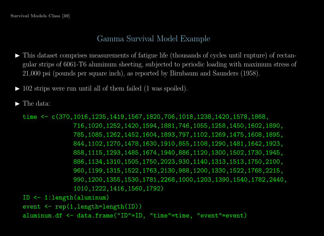
Gamma Survival Model Example

◮ This dataset comprises measurements of fatigue life (thousands of cycles until rupture) of rectan-

gular strips of 6061-T6 aluminum sheeting, subjected to periodic loading with maximum stress of

21,000 psi (pounds per square inch), as reported by Birnbaum and Saunders (1958).

◮ 102 strips were run until all of them failed (1 was spoiled).

◮ The data:

time <- c(370,1016,1235,1419,1567,1820,706,1018,1238,1420,1578,1868,

716,1020,1252,1420,1594,1881,746,1055,1258,1450,1602,1890,

785,1085,1262,1452,1604,1893,797,1102,1269,1475,1608,1895,

844,1102,1270,1478,1630,1910,855,1108,1290,1481,1642,1923,

858,1115,1293,1485,1674,1940,886,1120,1300,1502,1730,1945,

886,1134,1310,1505,1750,2023,930,1140,1313,1513,1750,2100,

960,1199,1315,1522,1763,2130,988,1200,1330,1522,1768,2215,

990,1200,1355,1530,1781,2268,1000,1203,1390,1540,1782,2440,

1010,1222,1416,1560,1792)

ID <- 1:length(aluminum)

event <- rep(1,length=length(ID))

aluminum.df <- data.frame("ID"=ID, "time"=time, "event"=event)



◮ The library flexsurv allows several different distributions to be specified, even custom distribu-

tions.

◮ Specify the model with a gamma distribution and get the parameters, plus a plot:

library(flexsurv)

aluminum.fit <- flexsurvreg(Surv(ID,time,event) ~ 1, dist="gamma",

data=aluminum.df)

aluminum.fit$coefficients

shape rate

2.47275 -4.77213

plot(aluminum.fit)


Discrete Time Models

◮ Motivation: even though time is continuous, nonparametric estimation methods impose discrete-

ness.

◮ Any measure of time has to be discrete.

◮ Also, collectors of data often do not make time measurements highly granular, like measuring life

in years (generating ties).

◮ For the support:

r1, r2, r3, . . . , rk

the random variable R has the PMF:

pi = p(R = ri), i = 1, . . . , k

with pi > 0, ∀i, and∑k

i=1 = 1.



◮ The cumulative hazard function is:

F (t) =∑

i:ri≤t

pi

(notice the “less than or equal:” i : ri ≤ t).

◮ The survival function is:

S(t) =∑

i:ri≥t

pi

(notice the “greater than or equal:” i : ri ≥ t).



◮ The hazard function is given by:

hi = p(R = ri|R ≥ ri) =pi

∑kj=1 pj

, i = 1, . . . , k

which only gives values bounded by [0 : 1].

◮ We can relate these functions, from recursion:

pi = hi

i−1∏

j=1

(1 − hj), i = 1, . . . , k

and substitute this into S(t) to get the discrete time survival function:

S(ri) =

k∑

j=1

pj =

i−1∏

j=1

(1 − hj)

with the general form:

S(t) =∏

j:rj<t

(1 − hj), t ≥ 0,

which is clearly decreasing in t.


Definition of the Geometric Distribution

◮ PMF: GEO(x|p) = p(1 − p)x−1, x = 1, 2, . . . , 0 ≤ p ≤ 1.

◮ E[X ] = 1p.

◮ Var[X ] = 1−pp2 .

0.00

0.05

0.10

0.15

0.20

0.25

1 2 3 4 5 6 7 8 9 10 11 12 13 14 15 16 17 18 19 20 21 22 23 24


The Geometric Distribution

◮ The geometric distribution can be thought of as the discrete version of the exponential distribution.

◮ It has support on 1, 2, . . . (sometimes defined to include zero) rather than > 0.

◮ Like the exponential distribution, the gamma also has a constant hazard function:

hi = h, 0 < h < 1, i = 1, 2, . . .

(no aging).

◮ The PMF is:

pi = h(1 − h)i−1

◮ The survival function is then:

S(t) = (1 − h)⌊t⌋, t ≥ 0

Note that ⌊t⌋ is more appropriate than the Brostrom book’s version.


Geometric Distribution with h = 0.25


Hazard Atoms

◮ First define the risk set at duration t as R(t) = the set of all cases still alive just prior to time t.

◮ This definition accounts for cases that have have an event at t or are right censored at exactly

time t.

◮ The Brostrom book’s example is:

R(1) = {1, 2, 3, 4, 5}

R(4) = {1, 3}

R(6) = {3}

◮ Assuming the probability of an event when none happened is zero, count events and divide by the

size of the risk set gives the hazard atoms:

h(1) =1

5= 0.2

h(4) =1

2= 0.5

h(6) =1

1= 1.0


Cumulative Estimators

◮ Hazard items are not very revealing without some form of smoothing (kernel smoothers, etc).

◮ Denote h(s) as the hazard atom at time s, with estimate h(s).

◮ The Nelson-Aalen estimator is:

H(t) =∑

s≤t

h(s), t ≥ 0

which gives a upward stairstep diagram (Brostrom Figure 2.8).

◮ The Kaplan-Meier estimator is:

S(t) =∏

s<t

(1 − h(s)), t ≥ 0

which gives a downward stairstep diagram (Brostrom Figure 2.9).


Application

◮ Back to the mort dataset:

lapply(c("eha","survival"),library, character.only=TRUE)

data(mort)

mort[1:10,]

id enter exit event birthdate ses

1 1 0.000 20.000 0 1800.010 upper

2 2 3.478 17.562 1 1800.015 lower

3 3 0.000 13.463 0 1800.031 upper

4 3 13.463 20.000 0 1800.031 lower

5 4 0.000 20.000 0 1800.064 lower

6 5 0.000 0.089 0 1800.084 lower

7 5 0.089 20.000 0 1800.084 upper

8 6 0.000 20.000 0 1800.094 upper

9 7 0.000 3.388 0 1800.105 upper

10 7 3.388 14.063 1 1800.105 lower

◮ Here event means: 1 for died during the period of study, and 0 means right censored.


Application: Nonparametric Estimation

◮ Create both the Nelson-Aalen and the Kaplan-Meier plots:

par(mfrow=c(1,2),mar=c(3,3,3,1),oma=c(1,1,1,1),col.axis="white",

col.lab="white", col.sub="white",col="white",bg="slategray")

with(mort, plot(Surv(enter, exit, event), fn = "cum"))

abline(h=0,col="slategray",lwd=5)

with(mort, plot(Surv(enter, exit, event), fn = "surv",ylim=c(0.6,1.0)))

◮ The definition of duration here starts at the age each man turns 20, until age 40 or death (about

22%).


Application: Graph of Nonparametric Estimation

0 5 10 15 20

0.00

0.05

0.10

0.15

0.20

0.25

0.30

0.35

Cumulative hazard function

Duration

0 5 10 15 20

0.6

0.7

0.8

0.9

1.0

Survivor function

Duration


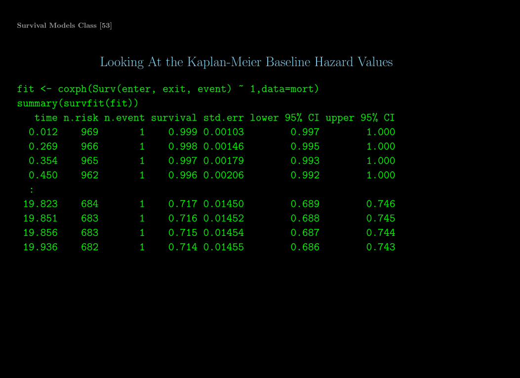
Looking At the Kaplan-Meier Baseline Hazard Values

fit <- coxph(Surv(enter, exit, event) ~ 1,data=mort)

summary(survfit(fit))

time n.risk n.event survival std.err lower 95% CI upper 95% CI

0.012 969 1 0.999 0.00103 0.997 1.000

0.269 966 1 0.998 0.00146 0.995 1.000

0.354 965 1 0.997 0.00179 0.993 1.000

0.450 962 1 0.996 0.00206 0.992 1.000

:

19.823 684 1 0.717 0.01450 0.689 0.746

19.851 683 1 0.716 0.01452 0.688 0.745

19.856 683 1 0.715 0.01454 0.687 0.744

19.936 682 1 0.714 0.01455 0.686 0.743


Parametric Estimation

◮ A “parametric proportional hazards model with no covariates.”

◮ Use phreg which uses the Weibull distribution as a default:

fit.w <- phreg(Surv(enter, exit, event) ~ 1, data=mort)

par(mfrow=c(1,2),mar=c(3,3,3,1),oma=c(1,1,1,1),col.axis="white",

col.lab="white", col.sub="white",col="white",bg="slategray")

plot(fit.w, fn = "cum")

plot(fit.w, fn = "sur",ylim=c(0.6,1.0)) # NOTE: "sur" NOT "surv"


Application: Graph of Weibull Estimation

0 5 10 15 20

0.00

0.05

0.10

0.15

0.20

0.25

0.30

Weibull cumulative hazard function

Duration

Cum

ulat

ive

Haz

ard

0 5 10 15 20

0.0

0.2

0.4

0.6

0.8

1.0

Weibull survivor function

Duration

Sur

viva

l


Weibull PDF

◮ PDF: w(x|γ, β) = γβxγ−1 exp

(

−(

xβ

)γ)

if x ≥ 0 and 0 otherwise, where: γ, β > 0.

◮ E[Xij] = βΓ[

1 + 1γ

]

.

◮ Var[Xij] = β2

(

Γ[

1 + 2γ

]

− γ[

1 + 1γ

]2)

0 2 4 6 8 10

0.0

0.2

0.4

0.6

0.8

1.0

γ = 0.5, β = 1

γ = 2, β = 3


Weibull Survival

◮ The Weibull distribution is more flexible than the exponential or gamma, and therefore more useful

for modeling survival data.

◮ This extra flexibility is achieved with an additional parameter, λ, which serves as a positive scale

parameter.

◮ The hazard function is given by:

h(t) = λp(λt)p−1

where t, λ, p > 0.

◮ The baseline hazard for the Weibull can be monotonically increasing (p > 1), monotonically

decreasing (p < 1), or flat (p = 1, like the exponential) with respect to time.

◮ The density function is given by:

f(t) = λp(λt)p−1 exp(−(λt)p).

◮ The survivor function is simply:

S(t) = exp(−(λt)p).


Weibull Survival

◮ The mean survival time (expected life) is:

E(t) =Γ(1 + 1

p

λ.

◮ The percentiles of duration times are given by:

t(p’tile) = λ−1 log

(

100

100 − p’tile

)1

p

where t(p’tile) is the percentile of interest. So the median survival time is calculated by:

t(50) = λ−1 log

(

100

100 − 50

)1

p

= λ−1 log(2)1

p .


The Weibull Survival Model

◮ The parametric Weibull model is specified by linking the single parameter to a linear additive

structure.

◮ For the full sample:

log(T ) = Xβ + σǫ

where σ is a scale parameter applied to ǫ which is a residual vector who’s components are

distributed Type-I extreme value (Gumbel):

f(ǫ|µ, β) =1

βexp((ǫ − µ)/β) exp[− exp((ǫ − µ)/β)]

where µ is the location parameter and β is the scale parameter. The standard form of the

PDF with µ = 0 and β = 1 is f(ǫ) = exp(ǫ) exp(− exp(ǫ)), and the corresponding CDF is

F (ǫ) = exp(− exp(ǫ)).

◮ This model is sometimes called an accelerated failure time (AFT) model because the log function

on the LHS means that there is an exponential on the RHS around the linear additive component.



−6 −4 −2 0 2 4 6

0.00.1

0.20.3

x

exp(x)

* exp(−

exp(x))

Gumbel PDF

−6 −4 −2 0 2 4 6

0.00.2

0.40.6

0.81.0

x

1 − ex

p(−exp

(x))

Gumbel PDF



◮ The Weibull regression model can also be expressed differently as a proportional hazards model:

h(t|x) = h0t exp(x1β1 + · · · + xkβk)

where the baseline hazard is h0t = exp(β0)ptp−1.

◮ More compactly, this is:

h(t|x) = ptp−1 exp(xβ)

where p is the Weibull shape parameter, and λ = exp(xβ) is the Weibull scale parameter.


Weibull Model of UN Peacekeeping Missions

◮ The data durations of United Nations peacekeeping missions from 1948 to 2001 (BSJ pages 27-31,

originally from Green, Kahl, and Diehl [1998]).

◮ There is one explanatory variable with three categories: civil war, interstate conflict, and interna-

tionalized civil war (the baseline category).

◮ The estimates in BSJ are MLEs from Stata where they run the exponential model, the Weibull

AFT model, and the Weibull proportional hazards model.

◮ Since the exponential model is the Weibull model with p = 1 we can test the nested model

difference.



◮ Since the Weibull reduces to the exponential when p = 1 (equivalently σ = 1), then we can test

for time dependency: the exponential assumes flat/constant hazard and the Weibull does not.

◮ This test is given by:

z =p − 1

SE(p)=

0.807 − 1

1.774= −1.93,

where p = 0.807 (rounded in the table) with SE(p) = 1.774 (not reported in the book).

◮ Therefore there is evidence that p < 1 (so σ > 1), meaning that the hazard rate is decreasing over

time.

◮ The interpretation is that the longer UN peacekeeping lasts, the lower the risk of it terminating.



◮ The biggest contrast in Table 3.1 is between the two Weibull specifications where:

⊲ The AFT model is linear for log(T ) so a positive coefficient is indicative of longer durations

for increasing values of the explanatory variable.

⊲ Conversely, the proportional hazards model explains the hazard rate, so positive coefficients

imply greater hazard with increasing values of the explanatory variable.

◮ For example the Civil coefficient in the AFT model is −1.10, which can be transformed to the PH

version by:

−(−1.10)/σ = 0.89.


Back To Censoring in BSJ Terminology

◮ We saw that the hazard rate, h(t), can be expressed as the ratio of the PDF to the survival

function, and this can be expressed in the form of definite integrals:

h(t) =f(t)

S(t)=

∫ t+∆t

t f(u)du∫ ∞

t f(u)du

which is the ratio of unconditional failure to survival.

◮ In practical situations the upper limit of the integral in the survival function is not ∞, but is some

time point set by the study, which forms the known right censoring point:

S(t) =

∫ t=Ci

t

f(u)du

for the ith case.

◮ For the left censoring case, we don’t have a survivor function in this context since S(t) = 1−H(t)

is undefined (BSJ are wrong here and also confuse censoring versus truncation).


Censored Data Likelihood Function

◮ Suppose we have n cases all with observed events ti (no censoring), then the likelihood function

is imply the product of the relevant PDF:

L =

n∏

i=1

f(ti).

◮ Now there are some cases that that live past the time the study ends, t∗, so the likelihood function

is now:

L =

n∏

ti≤t∗

f(ti)

n∏

ti>t∗

S(ti),

so that the uncensored cases contribute information to the likelihood function through event

times, and the censored cases contribute information only through the survival function at the

end-point.

◮ Note: on page 18 BSJ confusingly switch between t∗ and t∗i . Indexing by cases implies a more

complex research design, which have not yet encountered.


Censored Data Likelihood Function

◮ This can be further clarified through a standard re-expression of the likelihood function.

◮ Start with defining a non-censoring indicator function:

δi =

{

1 if ti ≤ t∗

0 if ti > t∗

◮ Now the likelihood function for data with censoring can be expressed with a single product as:

L =

n∏

i=1

{f(ti)}δi {S(ti)}

1−δi

which shows the bias imposed by omitting right censored cases.


Assignment for Week 3

1. Reproduce Figure 3.1 in Box-Steffensmeier and Jones. Note that this requires rerunning the

models.

2. Run a Kaplan-Meier analysis with your data.

3. Submit the data for your empirical paper.

Survival Models for the Social and Political Sciences Week 3: … · 2017-02-06 ·...

Documents

Transcript of Survival Models for the Social and Political Sciences Week 3: … · 2017-02-06 ·...