1

Survival, danger perception

and the amygdala

R A G U R A M R A V I S H A N K A R A N

Master of Science Thesis in Medical Engineering/Medical Imaging

Stockholm 2012

II

III

This master thesis project was performed in collaboration with

CIBM, EPFL

Supervisor at CIBM, EPFL: Wietske Van Der Zwaag

Survival, danger perception and the amygdala

R A G U R A M R A V I S H A N K A R A N

Master of Science Thesis in Medical Engineering/Medical Imaging

Advanced level (second cycle) 30credits

Supervisor at KTH: Anna Bjällmark

Examinator: Massimiliano Colarieti Tosti

School of Technology and Health

TRITA-STH. EX 2012:04

Royal Institute of Technology

KTH STH

E-141 86 Flemingsberg, Sweden

http://www.kth.se/sth

IV

i

Abstract

Fear is an emotion expressed by a subject which is under a threat or danger to secure itself. It

causes the “Fight or Flight” sensation in the being which is under attack. In previous studies,

it is found that amygdala is the central unit in brain for fear stimuli. Here we have done two

different neuroscience studies on fear with ultra high field MRI.

Case 1: With ultra high field MRI brain images we visualised that there is a faster and short

pathway to amygdala. Fear stimuli activate the amygdale even when the images are shown for

a very short time of 50ms with which conscious recognition is not possible. This shows brain

reacts to fear even before we recognise it consciously.

Case 2: We investigated the influence of low and high spatial frequency fearful images in

amygdala because of the contradiction in some previous studies. We compared low, high and

broad spatial frequency images of fearful averted gaze faces, snakes and objects and found

both high and low spatial frequency fear images affect the amygdale in the similar manner.

ii

Acknowledgements

I would like to express my heartfelt gratitude to my supervisor Wietske Van Der Zwaag,

who gave this delightful opportunity for me to undertake this project and learn so much

through it. Her support was of high value and it enabled me to understand details in depth and

finish my thesis work in time.

Many thanks to Nouchine hadjikhani, a constant support during my time in EPFL. The help

she provided at regular intervals during the thesis work solved my questions and made me

move forward.

Thanks to CIBM and EPFL for allowing me to be a part of the cutting edge technology. I

was exposed to the best technology that is available currently and I consider it as a privilege.

Also, thanks to the faculty members of CIBM who helped in running the instruments and

other needed aids.

My sincere thanks to Anna Bjällmark, who accepted the request to be my internal supervisor

and Massimiliano Colarieti Tosti, who agreed to be the internal examiner.

I’m very much grateful to Anna Helberg Gustafsson and Lena Salomonson, who gave the

necessary help and assistance with the paperwork regarding Erasmus exchange programme in

time for me to proceed with the thesis work, without that it would have been a struggle.

Finally, thanks to all my friends and well-wishers. For they supported me and helped me walk

miles with smile and confidence.

Stockholm, Sweden

Raguram Ravi Shankaran

iii

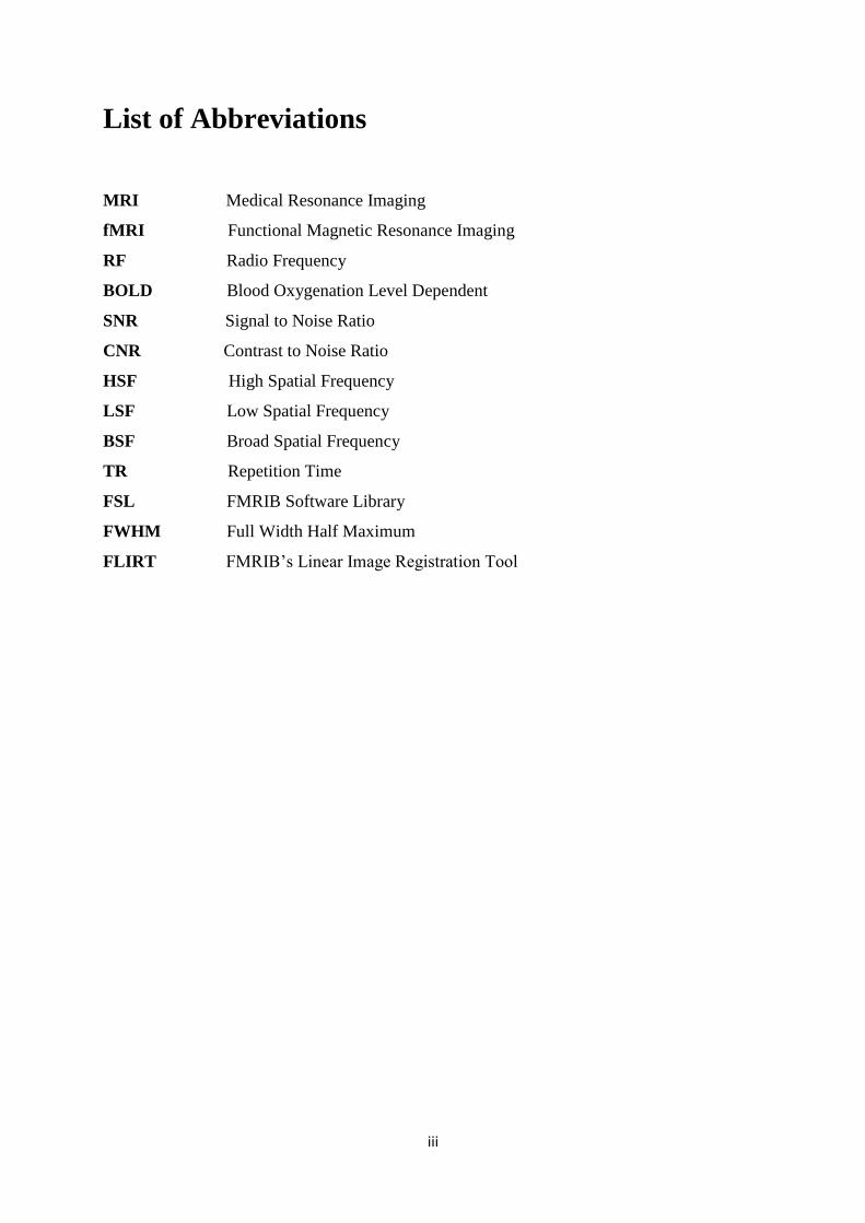
List of Abbreviations

MRI Medical Resonance Imaging

fMRI Functional Magnetic Resonance Imaging

RF Radio Frequency

BOLD Blood Oxygenation Level Dependent

SNR Signal to Noise Ratio

CNR Contrast to Noise Ratio

HSF High Spatial Frequency

LSF Low Spatial Frequency

BSF Broad Spatial Frequency

TR Repetition Time

FSL FMRIB Software Library

FWHM Full Width Half Maximum

FLIRT FMRIB’s Linear Image Registration Tool

iv

List of Figures

Figure 1.1 (a) Medial view of the brain showing one of the amygdale [2], (b) Brain showing both the

amygdalae [3] .......................................................................................................................................... 1

Figure 1.2(a) Nuclei with non zero magnetic moments [4] ..................................................................... 2

Figure 1.2 (b) Net Magnetization: i) the magnetic spins are random and the net magnetization is zero,

ii) spins are aligned with the external magnetic field B [5]. .................................................................... 3

Figure 1.2 (c) MRI images ........................................................................................................................ 3

Figure 1.2.2 Brain showing activation maps [8].Colour Range: Red to yellow – Positive Values, Green

to blue – Negative Values ........................................................................................................................ 5

Figure 1.3 Siemens Magnetom – 7T MRI (CIBM, EPFL) ........................................................................... 6

Figure 1.3.1 32 channel head coil ............................................................................................................ 7

Figure 1.4.1 (a) Pathways to amygdala: The Subcortical pathway (blue line) via superior colliculus and

pulvinar nuclei is shown and the cortical pathway (purple line) to amygdala includes Lateral

geniculate nucleus (LGN) and the primary visual cortex of the brain. .................................................... 8

Figure 1.4.1 (b) Illustration of different visual pathways to amygdala based on LeDoux JE (1994)

Emotions, Memory and the Brain. Scientific American [15]. .................................................................. 9

Figure 2 A subject on a 7T MRI couch at CIBM, EPFL [19] .................................................................... 11

Figure 2.1 1(a), 1(b) – Pleasant animals and Fig 2(a), 2(b) – Fearful animals ................................. 12

Figure 2.1.1 (a) Overt and Subliminal run Model. ................................................................................. 13

Figure 2.1.1 (b) Example of a Block: It is a fear block of 27 seconds ..................................................... 13

Figure 2.1.2 (c) Overt Run...................................................................................................................... 13

Figure 2.1.2 (d) Subliminal Run ............................................................................................................. 14

Figure 2.2 Example of images used in “effect of spatial frequency on amygdala” ............................... 15

Figure 2.2.1 (a) Spatial Filtering ............................................................................................................. 16

Figure 2.2.1 (b) Face, Snake and Object in different spatial frequency versions .................................. 17

Figure 2.2.2 (a) BSF, HSF and LSF stimuli model .................................................................................... 18

Figure 2.2.2 (b) BSF Run ........................................................................................................................ 18

Figure 2.2.2 (c) LSF Run ......................................................................................................................... 19

Figure 3 FSL GUI window showing various tools for MRI image analysis ............................................. 20

Figure 3.1.1 (a) First level FEAT analysis ................................................................................................ 21

Figure 3.1.1 (b) Full model setup of overt/subliminal stimuli showing their EVs and Contrasts setup. 22

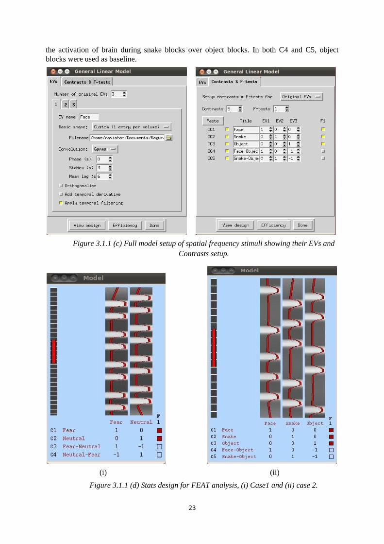
Figure 3.1.1 (c) Full model setup of spatial frequency stimuli showing their EVs and Contrasts setup.

............................................................................................................................................................... 23

Figure 3.1.1 (d) Stats design for FEAT analysis, (i) Case1 and (ii) case 2. .............................................. 23

Figure 3.1.1 (e) Registration .................................................................................................................. 24

Figure 3.1.2 FEAT – Higher level analysis .............................................................................................. 25

Figure 3.2 FSL View ................................................................................................................................ 26

Figure 4.1.1 (a) Overt Stimuli: Left amygdala (marked with yellow circle) showing activation ............ 27

Figure 4.1.1 (b) Overt Stimuli: Showing activation on pulvinar and superior colliculus (region within

yellow circle) .......................................................................................................................................... 28

Figure 4.1.2 Subliminal stimuli: Showing activation on left amygdale (region within yellow circle) .... 29

Figure 4.2.1.1 (a) BSF Face: Showing activation on right and left amygdale (marked with yellow circle)

............................................................................................................................................................... 30

v

Figure 4.2.1.1 (b) BSF Face: showing activation on superior colliculus and pulvinar (marked with

yellow circle) .......................................................................................................................................... 31

Figure 4.2.1.2 (a) BSF Snake: Showing activation on left amygdale (marked with yellow circle) ......... 32

Figure 4.2.1.2 (b) BSF Snake: showing activation on superior colliculus and pulvinar ........................ 32

Figure 4.2.2.1 HSF Face: Showing activation on right and left amygdala ............................................ 33

Figure 4.2.2.2 HSF Snake: Showing activation on left amygdala ........................................................... 34

Figure 4.2.3.1 LSF Face: Showing activation on both right and left amygdala ..................................... 35

Figure 4.2.3.2 LSF snake: Showing activation on left amygdale ........................................................... 36

vi

Contents Abstract ......................................................................................................................... i

Acknowledgements ..................................................................................................ii

List of Abbreviations ............................................................................................ .iii

List of Figures............................................................................................................iv

1. Introduction ........................................................................................................... 1

1.1 Amygdala .......................................................................................................................... 1

1.2 Magnetic Resonance Imaging (MRI) ................................................................................ 2

1.2.1 Functional Magnetic Resonance Imaging (fMRI).................................................................... 4

1.3 Ultra high field magnetic resonance imaging (7T MRI).................................................... 6

1.4 Previous research on fear stimuli...................................................................................... 8

1.4.1 Evidence of subcortical pathway ............................................................................................ 8

1.4.2 Effect of different spatial frequency on amygdale ................................................................. 9

1.5 Aim .................................................................................................................................. 10

2. Methods ................................................................................................................ 11

2.1 Case 1: Overt and Subliminal Stimuli .............................................................................. 11

2.1.1 Design ................................................................................................................................... 12

2.2 Case 2: Effect of spatial frequency.................................................................................. 14

2.2.1 Spatial Filtering ..................................................................................................................... 14

2.2.2 Design ................................................................................................................................... 18

2.3 Procedure ........................................................................................................................ 19

2.3.1 Overt and Subliminal run ...................................................................................................... 19

2.3.2 Effects of spatial frequency .................................................................................................. 19

3. Data Processing ................................................................................................. 20

3.1 FEAT FMRI analysis ......................................................................................................... 21

3.1.1 First Level Analysis ................................................................................................................ 21

4.1.2 Higher level analysis ............................................................................................................. 25

3.2 FSL View .......................................................................................................................... 25

4. Results ................................................................................................................... 27

4.1 Case 1 – Overt and Subliminal stimuli ............................................................................ 27

4.1.1 Overt ..................................................................................................................................... 27

vii

4.1.2 Subliminal stimuli ................................................................................................................. 28

4.2 Case 2 - Effect of spatial frequency in fear stimuli ......................................................... 30

4.2.1 Broad Spatial Frequency (BSF) stimuli .................................................................................. 30

4.2.2 High Spatial Frequency (HSF) stimuli .................................................................................... 33

4.2.3 Low Spatial Frequency (LSF) stimuli ..................................................................................... 35

5. Discussion and Conclusion ............................................................................ 38

5.1 Fear Overt and Fear Subliminal ...................................................................................... 38

5.2 Effect of different spatial frequency for fear stimuli ...................................................... 38

5.3 Conclusion ....................................................................................................................... 39

Bibliography ............................................................................................................ 40

1

1. Introduction

Fear is an unpleasant sensation caused by the presence of danger or perceived threat. It is a

defensive emotion which motivates organisms to cope with different type of survival threats

throughout evolution. If there is a harm or survival threat, fear enables the body to produce an

inborn, automatic response which prepares the body to “fight” or “flee”. This response is

called “fight or flight response”. In short, the critical purpose of fear is to save lives. The

amygdalae are the regions of the brain which process fear stimuli [1].

1.1 Amygdala

Amygdala is a tiny almond-shaped structure located deep within the medial temporal lobes of

the brain (Figure 1.1 (a)). There are two amygdalae as shown in Figure 1.1 (b) located

adjacent to the hippocampus. The processing of emotions such as fear, pleasure and anger

takes place in the amygdala. The amygdala seems to be the central site of the fear module and

fear learning in humans [1]. These different brain activities can be measured using a Magnetic

Resonance Imaging (MRI) procedure called fMRI, a functional magnetic resonance imaging.

Figure 1.1 (a) Medial view of the brain showing one of the amygdale [2], (b) Brain

showing both the amygdalae [3]

2

1.2 Magnetic Resonance Imaging (MRI)

MRI is a medical imaging technique to produce high quality images of internal structures of

the body. It is based on the principles of nuclear magnetic resonance (NMR).

Like any spinning charged object, a nucleus with a non-zero spin creates a magnetic field

around it, which is analogous to the microscopic bar magnet. It is represented as a vector

quantity called the nuclear magnetic dipole moment or magnetic moment as shown in figure

1.2(a). The sum of all these tiny magnetic field of each spin is called net magnetization. It is

usually zero because all the individual spins are randomly distributed and cancels each other’s

magnetic field (Figure 1.2 (b) i) [4].

Figure 1.2(a) Nuclei with non zero magnetic moments [4]

When these particles are placed in a large magnetic field (B) it aligns with the magnetic field

B as shown in figure 1.2 (b) ii. Most of the spins align parallel with the magnetic field and

few align anti-parallel and hence there will be a net magnetization [5]. MRI machines make

use of this principle that body tissue contains lot of water and hence hydrogen nuclei, which

gets aligned in large magnetic field.

3

Figure 1.2 (b) Net Magnetization: i) the magnetic spins are random and the net

magnetization is zero, ii) spins are aligned with the external magnetic field B [5].

When a person is placed inside a MRI scanner, the powerful magnetic field inside will align

most of the proton in the human body along the direction of its magnetic field. At this point a

electromagnetic radio frequency signal is applied at a certain frequency called resonance

frequency, which alters the direction of spin for a shorter period of time during which RF

wave is applied. After that they go back to the normal position which is to the direction of the

applied magnetic field. During this relaxation, a radio frequency signal is generated by these

particles which are acquired with the RF wave receiver. For this purpose radio frequency (RF)

coils are used. There are different types of RF coils for different parts of the body such as

head coils, body coils, breast coils, etc. It is then processed using Fourier transform to produce

the final MRI image. The pictures in Figure 1.2 (c) are the examples of MRI images. The

fMRI is one of the advanced imaging techniques of MRI and it measures brain activity.

Figure 1.2 (c) MRI images

4

1.2.1 Functional Magnetic Resonance Imaging (fMRI)

Functional magnetic resonance imaging (fMRI) is a novel technique for measuring brain

activation and works by detecting the changes in blood oxygenation and flow that occur in

response to neuronal activity. When a brain area is more active it utilizes more oxygen and to

meet the increased demand the blood flow increases and shows the area active. For example

when you move your left hand there is a rapid momentary increase in the circulation of the

specific part of the brain controlling that movement of the hand. Based on this principle fMRI

is used to produce activation maps that shows the region of particular neuronal activity [6].

Haemoglobin is paramagnetic when deoxygenated and becomes diamagnetic when

oxygenated. The change in the magnetic property of haemoglobin leads to small differences

in the MR signal. This difference in MR signal changes is proportional to level of

oxygenation in brain and this correlation is used to analyze different to functional process of

brain. This form of MRI is known as blood oxygenation level dependent (BOLD) imaging

[7].

The direction of oxygenation changes with increased activity. There is a decrease in blood

oxygenation immediately after neuronal activity increases, known as the ‘initial dip’ in the

haemodynamic response. This is followed by a period were the blood flow increases, not just

to a level where the oxygenation is met, but over-compensating for the increased demand.

This means the blood oxygenation actually increases following neuronal activation. The blood

flow peaks after 6 seconds, then falls back to baseline [7].

Activation maps

There are many kinds of fMRI stimuli such as visual, auditory, sensory stimuli, etc. For

example, the subject lying in the MRI scanner would watch a screen which alternated between

showing a visual stimulus and being dark every 45 second. During this stimulus the MRI

scanner tracks the signal throughout the brain. In brain areas responding to the visual

stimulus, the signal goes up and down as the stimulus is turned on and off (Dark), although

blurred slightly by the delay in the blood flow response. The ‘activity’ in a voxel is defined by

how closely the signal from that voxel matches the visual stimulus over the time. I.e. how

closely the signal goes up when the stimulus is turned on and vice versa. Voxels whose signal

corresponds tightly to the model are given high activation scores, voxels showing no

correlation have a low score and voxels showing the deactivation are given a negative score.

These are then translated into activation maps [8]. From figure 1.4.1, activation map of a

Brain can be observed, showing different colours, indicating positive and negative values.

5

Figure 1.2.2 Brain showing activation maps [8].Colour Range: Red to yellow –

Positive Values, Green to blue – Negative Values

6

1.3 Ultra high field magnetic resonance imaging (7T MRI)

MRI opens up unique possibilities to study the functional changes in the human brain during

fear perception.

Field strength of MRI ranges from 0.2 to 14.1 Tesla. For clinical purpose the field strength of

MRI ranges from 0.2 to 3 Tesla. The MRI with field strength of 3T and above are called ultra

high field MRI. We used ultra high field 7T MRI scanner for our research. We choose 7T

MRI because as the field strength increases the spatial resolution increases.

The ultra high field 7 Tesla MRI scanner, very few in numbers throughout the world, is

currently used only for research purpose. It has not yet been in market commercially for

diagnostic purpose. Ultra-high spatial resolution images are possible with 7T MRI scanners. It

is even easy to observe and analyze the tissue metabolism and function.

The main application area of 7T MRI is functional MRI. In future, it is expected to have the

potential to study the neuronal function at sub-millimetre scale [9]. Its major clinical

application is in the study of neurodegenerative diseases like Alzheimer’s disease [10]. At

present the main focus of ultra-high field MRI is on brain imaging.

Functional MRI at ultra-high field/7T has a high signal-to-noise (SNR) and contrast-to-noise

(CNR) ratio. With this feature contrast-rich images can be produced for diagnosing severe

pathological issues like multiple sclerosis, cerebrovascular disease, brain tumors and aging

related disease [11]. Figure 1.3 shows the image of the 7T MRI that was used for this project

at CIBM, EPFL.

Figure 1.3 Siemens Magnetom – 7T MRI (CIBM, EPFL)

7

Head coil

Head coil is a radio frequency (RF) coil used to transmit and receive RF signals from the

head.

Out of several head coils, used in the MRI scanner we have used a 32 channel head coil to

take the brain images. The 32 channel head coil has advantages over other head coils such as

high signal to noise ratio (SNR) and image homogeneity. Due to the high number of coil

elements in the 32 channel coil, parallel imaging performance is better. The helmet shaped

geometry of this coil makes the acceleration possible in any direction [12].

The head coil has detachable view mirrors as shown in Figure 1.3.1 through which video and

image displays are viewed inside the magnet for visual experiments. The visual stimuli from

the computer were sent to the projector which is placed behind the scanner room. It projects

the visuals through a tube onto a plastic screen placed inside the magnet. The subjects can see

the screen through the view mirrors.

There are some disadvantages of the 32 channel head coil. Because of its helmet shaped and

limited diameter size, larger heads cannot be scanned with this coil. Also the image

reconstruction takes a long time with this coil because large number of data volume has to be

processed when compared with other lesser channel head coils [12]. Figure 1.2.1 shows the 32

channel head coil that was used for the experiment.

Figure 1.3.1 32 channel head coil

8

1.4 Previous research on fear stimuli

1.4.1 Evidence of subcortical pathway

Recent studies found that the amygdale is activated by fear stimuli, even when conscious

recognition is prevented by backward masking [13]. Backward masking is a phenomenon in

cognitive psychology where a visual stimulus (Masking Image – Refer Figure 2.1.2 (d)) is

presented soon after the brief (≤ 50ms) presentation of “target” visual stimulus (here fear

stimuli) leads to a failure to consciously perceive the first stimulus [14]. They added that the

activation of the amygdala has another subcortical pathway with which amygdala can be

activated in the absence of cortical processing. The subcortical pathway is via the superior

colliculus and the pulvinar nuclei of the thalamus. This unconscious route to amygdale is

much faster than the normal cortical pathway. This helps to react to danger before we see it

consciously. The different pathways to amygdala are shown in Figure 1.4.1 (a). Illustration of

normal conscious pathway and subcortical pathway can be seen from the figure 1.4.1 (b).

Figure 1.4.1 (a) Pathways to amygdala: The Subcortical pathway (blue line) via

superior colliculus and pulvinar nuclei is shown and the cortical pathway (purple

line) to amygdala includes Lateral geniculate nucleus (LGN) and the primary visual

cortex of the brain.

9

Figure 1.4.1 (b) Illustration of different visual pathways to amygdala based on

LeDoux JE (1994) Emotions, Memory and the Brain. Scientific American [15].

The above interesting study led us to investigate the subcortical pathway and amygdala with

ultra high magnetic field MRI. We used ultra-high field (7T) MRI to look at the amygdala

because we could gain additional information about the different nuclei of that structure that

are not readily seen at lower field.

It was also important to test that our protocol was giving good signal in the amygdala, that is a

very delicate structure to image at 7T, and this is why we tried a protocol that had already

shown that it was successful at lower field.

1.4.2 Effect of different spatial frequency on amygdale

High and low spatial frequency information in visual images is processed by distinct neural

channels. Examples of high spatial images and low spatial images are shown in Figure 2.2.1

(b). Using event-related functional magnetic resonance imaging (fMRI) in humans,

dissociable roles of such visual channels for processing faces and emotional fearful

expressions can be seen. One study [16] has shown that amygdala responses to fearful

expressions are preferentially driven by intact or low spatial frequency (LSF) images of faces,

rather than by high spatial frequency (HSF) images. In other words, amygdala responses to

fearful expressions were greater for low-frequency faces than for high-frequency faces. An

activation of pulvinar and superior colliculus by fearful expressions occurred specifically with

low-frequency faces, suggesting that these subcortical pathways may provide coarse fear-

related inputs to the amygdala. These results suggest that LSF components processed rapidly

via magnocellular pathways within the visual system might be very efficiently conveyed to

the amygdala for the rapid recognition of fearful expressions [16].

Subcortical Pathway

Conscious visual pathway

10

In another study [17], amygdala responses to fearful expressions were found to be

preferentially driven by intact low spatial frequency images in the brain imaging studies

conducted recently. Magnocellular pathways within the visual system via the sub cortical

pathway that activates the pulvinar and superior colliculus were found to enable rapid

recognition of fearful expressions by LSF as the HSF utilises the striate and temporal cortex

for the same. The research mainly focussed on comparing the facial expression via statistical

data in the LSF and HSF [17].

In contrast with the previous studies, a recent study [18] conducted with fearful facial

expressions presented at two different eccentric points and the facial expressions were filtered

on the basis of low or high frequencies. It was found that the amygdala responds in the same

manner in both LSF and HSF regardless of the fearful stimuli in the visual field [18].

This contrast in views led us to investigate the effects of different spatial frequency in

amygdala for fearful face images. To add more to this experiment, we added the images of

threatening and neutral objects and compared all the three (face, snake and objects).

1.5 Aim

To investigate more into the above interesting studies, two experiments were planned.

The first objective was to investigate the amygdale and subcortical pathway through overt and

subliminal stimuli using 7T MRI (case 1). The second objective was to compare, the

amygdala response to different spatial frequencies in faces, snakes and objects (case 2).

11

2. Methods The subject was placed as shown in the figure 2 with his head placed inside the helmet shaped

32 channel head coil (ref: Figure 1.2.1) and pushed slowly inside the scanner. The different

visual stimuli from the computer were projected onto a plastic screen placed inside the

magnet. It is done with the help of a projector which is placed behind the scanner room. The

subject viewed the image on the screen through the view mirror of the 32 channel head coil

(ref: Figure 1.2.1).

Figure 2 A subject on a 7T MRI couch at CIBM, EPFL [19]

The following explains the methods and designs for the two separate cases.

2.1 Case 1: Overt and Subliminal Stimuli

The subjects were exposed to two kinds of pictures (fearful and pleasant pictures) in two

separate stimuli.

1. Overt

2. Subliminal

There were 128 pictures of fearful animals and pleasant animals each. Among the fearful

animals 64 pictures were snakes and the other 64 were spiders. A mixture of different animals

such as dogs, cats etc have been used as pleasant animals in the other set of 128 pictures.

Every picture was used in 300 × 300 pixel resolution. These pleasant animals/pictures were

named as Neutral pictures.

12

1(a) 1(b)

2(a) 2(b)

Figure 2.1 1(a), 1(b) – Pleasant animals and Fig 2(a), 2(b) – Fearful animals

2.1.1 Design

The software e-Prime 2.0 was used to design the stimuli.

The stimuli were designed in such a way that each subject was exposed to 21 blocks with 27

seconds each. An example of a block is shown in the Figure 2.1.1 (b). The design consists of

three different block types which were ‘N’ containing a series of different neutral pictures, ‘F’

containing a series of different fearful pictures and ‘R’ meaning a rest block containing a

white cross on a black background.

The paradigm was designed in such a way that the stimuli start with rest block(R) followed by

four blocks containing N and F alternatively, and ending with R. This particular design is

repeated four times so that the design attains 21 blocks in total as shown in the figure 2.1.2

(a).

13

Figure 2.1.1 (a) Overt and Subliminal run Model.

Figure 2.1.1 (b) Example of a Block: It is a fear block of 27 seconds

In the overt run, the main image was presented for 300 milliseconds (ms) followed by

fixation cross image for 1200 milliseconds as shown in Figure 2.1.2 (c). So in each of these

27 second blocks, 18 such images were presented (refer: Figure 2.1.1 (b)). The Figure 2.1.2

(c) shows one set of image in the fear block. In a neutral block, pleasant animals were

presented in the same way.

300ms 1200ms

Figure 2.1.2 (c) Overt Run

14

In the subliminal run, the main image was presented for just 50ms and then presented with

masking image for 250ms followed by 1200ms fixation cross image as shown in Figure 2.1.2

(d).18 such images were presented in 27 second block as in the overt run. The minimum time

required by the brain to see an image consciously would lie in the range 60ms – 70ms and the

50ms exposure to the image in this method being small, makes it subliminal.

50ms 250ms 1200ms

Figure 2.1.2 (d) Subliminal Run

2.2 Case 2: Effect of spatial frequency

The brain activity towards fearful faces, snakes and objects in different spatial frequencies

were also compared as a part of this experiment.

This was achieved by using averted gaze faces of 4 men and 3 women. Each face has two

different gazes one to the right and one at left. Faces were isolated from background and these

images were obtained from the Brain mind institute, EPFL. In total 14 pictures of faces were

used in this experiment.

16 different snake images were used for the pictures of snakes and 16 images including chair,

water bottle, table, etc have been used as object as explained in the Figure 2.2. It can be seen

that these images had their background removed as well using Adobe Photoshop.

The images used were all black-and-white and their luminances were corrected between 150-

160 levels on a 256 grey-scale level using Matlab.

All these normal images were used as broad spatial images.

2.2.1 Spatial Filtering

Broad spatial frequency images (BSF) were filtered into low spatial frequency and high

spatial frequency images using Matlab. Images were converted into their frequency domain

using fourier transform and subsequently multiplied with low pass and high pass filters with

cut-off frequency >7 cycles per image and < 30 cycles per images for the LSF and HSF

respectively which can be seen in Figure 2.2.1 (a). Finally, the inverse fourier of the filtered

Masking Image

15

frequency domain image gives the LSF and HSF images, the examples of which are shown in

Figure 2.2.1 (b).

Figure 2.2 Example of images used in “effect of spatial frequency on amygdala”

16

Gray Scale Image Frequency Domain

Frequency Domain High Pass Filter HSF Image

Frequency Domain Low Pass Filter LSF Image

Figure 2.2.1 (a) Spatial Filtering

IFFT

IFFT

FFT

T

17

BSF HSF LSF

Figure 2.2.1 (b) Face, Snake and Object in different spatial frequency versions

18

2.2.2 Design

As for the experiment 2.2, all the stimuli were designed using e-Prime 2.0.

There were 21 blocks of 18 seconds each. There were four kinds of blocks, starting with a rest

block and followed by a three functional blocks (Face, Snake & Object). The rest blocks at

regular intervals are to give more rest for subjects which will make them to focus at the

images even better. The model can be seen in Figure 2.2.2 (a).

Figure 2.2.2 (a) BSF, HSF and LSF stimuli model

BSF, HSF and LSF images have three separate runs like in the figure shown above. i.e A LSF

stimuli will have only the LSF images of faces, snakes and objects in all the functional blocks.

The rest block consist of a white cross at the centre of the black background and it does not

contain any images.

So in all these three stimuli, the main image was presented for 300ms followed by 1200ms

fixation cross image as shown in Figure 2.2.2 (b) and (c). So in each of these 18 second

blocks, 12 such images were presented.

300ms 1200ms

Figure 2.2.2 (b) BSF Run

19

300ms 1200ms

Figure 2.2.2 (c) LSF Run

2.3 Procedure

2.3.1 Overt and Subliminal run

5 subjects who were not phobic to any animals participated in the experiments for the overt

and subliminal runs. They were selected by the following approach. We placed an ad on

EPFL university website stating that the project requires volunteers who are phobic to one or

more animals and volunteers who are not phobic to any animals. If they are phobic, they were

asked to mention which animal they are scared of. Now by stating that both the phobic and

non-phobic volunteers are required, people came out with the truth rather than trying to hide

out just for the sake of participating in our paid experiment. From the obtained list the non-

phobic were filtered out. This worked out effectively and a group of non-phobic subjects were

gathered. They were well instructed about the procedure and MRI. There were three sections

for these subjects. In the first section the anatomical image of the brain was taken. This lasted

about 7 minutes and the subjects were asked to relax during this time. The next two were the

functional runs with the overt and subliminal stimuli. Here the subjects were asked to focus

well at the focus cross and the images. Three subjects started with subliminal run and the

other two were started with overt.

2.3.2 Effects of spatial frequency

For this experiment, all the procedures followed were similar as above for overt and

subliminal runs but here 7 subjects were used and there were three functional runs with BSF,

LSF and HSF stimuli. Again, the runs were counterbalanced across subjects.

20

3. Data Processing All the post processing of the data was done using the software FMRIB software library

(FSL).

FSL is a comprehensive library of image analysis and statistical tools for processing FMRI,

MRI and DTI (Diffusion Tensor Imaging) brain imaging data. FSL is a non-commercial

software available for the Linux and Mac operating systems. Windows version is supported

via a Linux virtual machine. In this study, Linux operating system was used.

FSL uses NIFTI format for processing fMRI and MRI data. The data obtained from the 7T

MRI were converted into NIFTI format using software called MRIConvert.

From FSL software library, the following tools were used.

o FEAT FMRI Analysis

o BET brain extraction

o FSL View

Figure 3 FSL GUI window showing various tools for MRI image analysis

21

3.1 FEAT FMRI analysis

FEAT is a software tool with an easily accessible graphical user interface (GUI) for fMRI

data analysis. There are two types of analysis – first level and higher level analysis.

3.1.1 First Level Analysis

The entire subject’s fMRI data were individually analysed using first level analysis. The

FEAT GUI window will have many tabs and tools as shown in the figure 3.1.1 (a).

Data

Functional images were loaded with their respective TR-values and number of volumes. The

high pass filter cut-off was set to default value 100.

Figure 3.1.1 (a) First level FEAT analysis

Pre-stats

To remove the effect of subjects head motion during the experiment, motion corrections were

done. FSL employs MCFLIRT for this purpose.

22

Spatial smoothing was carried out on each of the fMRI data sets which improves signal-to-

noise ratio. It was set to 5mm FWHM (full width half maximum).

Stats

A model was designed for the functional runs under ‘full model setup’. Different model setup

was designed for case 1 and case 2.

For case 1, two explanatory variables (EV) named fear and neutral were created as shown in

Figure 3.1.1(b). Design files were created for fear and neutral EV’s and loaded in fear and

neutral EV’s respectively. These design files contained the timings of fear and neutral image

blocks presented during the experiment.

Four contrasts were designed as shown in the Figure 3.1.1(b). Contrast C1 codes for

activation during fear blocks alone. Contrast C2 codes for activation on brain during neutral

blocks alone and contrast C3 which is our contrast of interest shows the activation of brain

during fear blocks over neutral blocks. The contrast C4 (neutral over fear) is the opposite of

contrast C3.

Figure 3.1.1 (b) Full model setup of overt/subliminal stimuli showing their EVs and

Contrasts setup.

For case 2, three EVs named face, snake and object were created. Separate design files were

created for face, snake and object. Then it is loaded in face, snake and object EV’s

respectively. These design files contained the timings of face, snake and object image blocks

presented during the experiment.

Five contrasts were designed as shown in the Figure 3.1.1 (c). The contrast C1, C2, C3 shows

the activation on brain during face, snake and object alone respectively. The contrast C4

shows the activation of brain during face blocks over object blocks. The contrast C5 shows

23

the activation of brain during snake blocks over object blocks. In both C4 and C5, object

blocks were used as baseline.

Figure 3.1.1 (c) Full model setup of spatial frequency stimuli showing their EVs and

Contrasts setup.

(i) (ii)

Figure 3.1.1 (d) Stats design for FEAT analysis, (i) Case1 and (ii) case 2.

24

Registration

Registration has to be done for the multi-subject analysis. Each of the subject’s brain has their

own shape and size. Therefore it is difficult to compare their brain activation. So images of all

brains were registered to a standard brain image. Here it uses FLIRT (FMRIB’s Linear Image

Registration Tool) for this purpose. It is fully automated intra- and inter-modal registration

tool [20].

Registration method

The low resolution functional data of a subject was registered to the whole brain (initial

structural image) of the same subject. Then obtained image was registered to the main

structural image. The main structural image was the high resolution MP2RAGE image

obtained using BET (Brain Extraction Tool). BET deletes all the non-brain tissues from the

whole head leaving the brain alone [21].

Then this high resolution image was registered to a standard brain which is the default

reference image in FSL software. The standard brain used for this purpose was

MNI152_T1_2mm_brain.

Figure 3.1.1 (e) Registration

25

3.1.2 Higher level analysis

Here group analyses were done by combining all the individual FEAT results obtained in first

level analysis. The obtained result is called gfeat (Group FEAT). Feat results from five

subjects in case 1 and seven subjects in 2 were combined separately and their respective gfeat

were obtained. Lower-level copes are the contrasts obtained in first level analysis. The mean

of the subjects were obtained using this analysis.

Figure 3.1.2 FEAT – Higher level analysis

3.2 FSL View

FSL View is a GUI tool used to read and analyze various MRI images. The images can be

opened in ortho view, i.e. coronal, sagittal and axial views can be displayed simultaneously.

Sufficient information like position and orientation can be seen.

The first image loaded is called main image. We can overlay any number of images by adding

images to main image. But the overlay image should be of same dimension as the main

image. With this many images can be compared.

26

Results were viewed using this tool. The results obtained in group feat were overlaid on a

standard brain used during the registration. Atlas tools in the toolbar shows the region of the

brain where the cross-hair is placed.

Figure 3.2 FSL View

27

4. Results All these results are from the group analysis. Different colours are used in fMRI results to

show activation in various brain regions. But all the colours have the same positive value.

From the earlier research, it was expected fear stimuli activates amygdala. The subcortical

pathway to amygdala includes pulvinar nucleus and superior colliculus. The activation of

these regions would show that fear stimuli takes shorter subcortical pathway to amygdala.

The grading of the activation was performed by observing the size of activation in the targeted

region, greater the size more the activation.

4.1 Case 1 – Overt and Subliminal stimuli

4.1.1 Overt

From the overt run stimuli experiment, activation was found in the left amygdale, pulvinar

nucleus of the thalamus and also in the superior colliculus. The shown result was the

difference in activation of brain regions for the fear stimulating snake/spider images over the

pleasant neutral images.

Figure 4.1.1(a) shows the activation of left amygdala. The obtained picture shows the fear

stimuli activating amygdala as expected

Figure 4.1.1 (a) Overt Stimuli: Left amygdala (marked with yellow circle) showing

activation

28

Frigure 4.1.1(b) shows the activation of pulvinar and superior colliculus. The obtained picture

shows the fear stimuli taking the short and faster pathway to reach amygdala.

Figure 4.1.1 (b) Overt Stimuli: Showing activation on pulvinar and superior

colliculus (region within yellow circle)

4.1.2 Subliminal stimuli

From the subliminal run, the activation was found in the left amygdala. But the activation was

not as pronounced as the activation found in overt run. The results showed that there was no

activation in superior colliculus and pulvinar nucleus, which was against our expectation.

Figure 4.1.2 shows the activation of left amygdala. The obtained picture shows that

subliminal fear stimuli can activate amygdala.

29

Figure 4.1.2 Subliminal stimuli: Showing activation on left amygdale (region

within yellow circle)

From the result:

1. In the overt run, it clearly shows that fear stimuli activates amygdala. Activation on

superior colliculus and pulvinar shows that there is a shorter pathway to amygdala.

2. In subliminal run, however there was no activation in subcortical regions (superior

colliculus and pulvinar nucleus), activation on left amygdala (even when conscious

recognition were prevented) clearly shows that fear stimuli took some shorter route to

amygdale which prepares brain to act faster in danger.

30

4.2 Case 2 - Effect of spatial frequency in fear stimuli

For all the three stimuli (BSF, HSF and LSF), the contrast of “face over object” and “snake

over object” are discussed in the following paragraphs. For BSF results a threshold of 1.5

were used and for the LSF and HSF results a threshold of 1.2 were used to view results.

4.2.1 Broad Spatial Frequency (BSF) stimuli

4.2.1.1 BSF Face

For the contrast of BSF face over BSF object, good activation was found on both the left and

right amygdale. Also there was a good amount of activation on superior colliculus and

pulvinar.

Figure 4.2.1.1(a) shows the activation of both right and left amygdala and Figure 4.2.1.1(b)

shows the activation of pulvinar nucleus and superior colliculus.

Figure 4.2.1.1 (a) BSF Face: Showing activation on right and left amygdale (marked

with yellow circle)

31

Figure 4.2.1.1 (b) BSF Face: showing activation on superior colliculus and pulvinar

(marked with yellow circle)

4.2.1.2 BSF Snake

For the contrast of BSF snake over BSF object, the activation found only on left amygdala but

not on the right amygdala. But high level of activation on superior colliculus and pulvinar was

found.

Figure 4.2.1.2(a) shows the activation on left amygdala and Figure 4.2.1.2(b) shows the

activation of pulvinar nucleus and superior colliculus.

32

Figure 4.2.1.2 (a) BSF Snake: Showing activation on left amygdale (marked with

yellow circle)

Figure 4.2.1.2 (b) BSF Snake: showing activation on superior colliculus and

pulvinar

33

4.2.2 High Spatial Frequency (HSF) stimuli

4.2.2.1 HSF Face

For the contrast of HSF face over HSF object, activation on both the amygdala was found. But

there was no activation on the superior colliculus and pulvinar nuclei.

Figure 4.2.2.1 shows the activation of both right and left amygdala

Figure 4.2.2.1 HSF Face: Showing activation on right and left amygdala

4.2.2.2 HSF Snake

For the contrast of HSF snake over HSF object, activation was found only on the left

amygdala but not on the right amygdala, superior colliculus and pulvinar nuclei.

Figure 4.2.2.2 shows the activation on left amygdala only.

34

Figure 4.2.2.2 HSF Snake: Showing activation on left amygdala

35

4.2.3 Low Spatial Frequency (LSF) stimuli

4.2.3.1 LSF Face

For the contrast of LSF face over LSF object, activation was found on both the amygdale but

not on the subcortical regions (superior colliculus and pulvinar nuclei).

Figure 4.2.3.1 shows the activation of left amygdala and right amygdala.

Figure 4.2.3.1 LSF Face: Showing activation on both right and left amygdala

36

4.2.3.2 LSF Snake

For the contrast of LSF snake over LSF object, activation was found only on left amygdala

but not on the right amygdala and subcortical regions (superior colliculus and pulvinar

nucleus).

Figure 4.2.3.2 shows the activation on left amygdala only.

Figure 4.2.3.2 LSF snake: Showing activation on left amygdale

37

Table 1 – Effect of different spatial frequency on amygdala and subcortical regions.

Right amygdala

Left amygdala

Pulvinar Superior colliculus

Face over Object - BSF

Snake over Object - BSF

Face over Object - HSF

Snake over Object - HSF

Face over Object - LSF

Snake over Object - LSF

38

5. Discussion and Conclusion

5.1 Fear Overt and Fear Subliminal

Experiments were conducted to investigate the subcortical pathway to amygdala during fear

stimuli under ultra high field MRI. We used ultra-high field (7T) MRI to look at the amygdala

because we could gain additional information about the different nuclei of that structure that

are not readily seen at lower field. It was also important to test that our protocol was giving

good signal in the amygdala, that is a very delicate structure to image at 7T, and this is the

reason we tried a protocol that had already shown that it was successful at lower field MRI.

Fear inducing snake and spider images were presented to the subjects in two different

methods. The image was shown for 300ms in one method where the subjects can see the

image consciously and the response was measured. For the other method, the images were

shown for short time duration of 50ms; here the subjects could not see the images consciously

because of backward masking and minimal time exposure

It was expected for both the methods to have the stimulation at amygdala and in the regions of

subcortical pathway, which includes superior colliculus and pulvinar nucleus of the thalamus.

Because from the previous studies it was found that amygdala is activated even when

conscious recognition is prevented by backward masking [14].

As we expected there was activation at amygdala and subcortical pathway regions for the Fear

Overt method. However, for the fear subliminal method it was found activation only with the

amygdala and not with regions of subcortical pathway. Since, the time duration for fear

subliminal method is too short; it is not possible for the fear stimuli to take the normal cortical

pathway to reach amygdala. From the results it was inferred that fear stimuli takes other

subcortical pathway to reach amygdala. The activation with fear overt method was found to

be stronger than fear subliminal method.

5.2 Effect of different spatial frequency for fear stimuli

Because of the existing contradictory statements [16] [17] [18] concerning the effect of LSF

and HSF images in amygdala, it was required to study them in detail. Though each of the

study has different experiment design, it all deals with the effect of low and high spatial

frequency images on amygdala. Here we didn’t redo any of the previous experiment design.

We just did our own experiment design to study on the effects of different spatial frequency

images on amygdala because of the previous contradictory statements.

In our study, as expected BSF has stronger activation on amygdala than LSF and HSF

faces/snakes. Also activation in superior colliculus and pulvinar nucleus were seen in BSF

faces/snakes but not in LSF and HSF faces/snakes.

It was found that the amygdala reacts to both LSF and HSF images of faces/snakes in a

similar manner. The results obtained match the findings of Morawetz C, B. J. (2010) [18]

39

and against the view of other two papers, Vuilleumier P, A. J. (2003) [16] and Martial

Mermillod, P.V. (2009) [17] which claims that LSF faces has more information than HSF

images.

Interestingly, in both the experiments fear stimuli with snakes/spiders activates only the left

amygdala whereas the face activates both the left and right amygdala.

Arne Ohman et al [13] has used spider/snake images for fear stimuli and concluded that only

left amygdale gets activated. In 2003 study [22], phobia related pictures shown to the subjects

activated left amygdala alone. In another study, Jillian E. Hardee (2009) [23] found that left

amygdala is more active to fear stimuli (fearful eyes) than the right amygdala. She also stated

that right amygdale is activated to any change in the eye (gaze-shift) where left amygdale

responded only to fearful eyes. That might be the reason, that the averted gaze fearful faces in

our experiment activated both the amygdala and the other fear stimuli with snake/spider

pictures activated left amygdala alone.

5.3 Conclusion

The project enriched in understanding the factors that are responsible for activating the fear,

added to this, it was possible to comprehend the role of nonconscious processes in amygdala .

The outcome of the project provided details about how amygdala reacts to fear stimulating

images of different spatial frequency, such as BSF, HSF and LSF. The role of fear in guiding

attention could also be well understood with the observations made from the project.

40

Bibliography

1. Arne Öhman, S. M. (2002). Phobias and preparedness: the selective, automatic, and

encapsulated nature of fear. Biological Psychiatry , Volume 52, Issue 10 , Pages 927-

937.

2. Myers, A. L. (2000). amygdala. Retrieved from memorylossonline:

http://www.memorylossonline.com/glossary/amygdala.html

3. Robin.H. (n.d.). Retrieved from

http://en.wikipedia.org/wiki/File:Constudoverbrain.png

4. Boch, F.(1971). Signal generation and detection. In Zhi-pei Liang, Paul .C.L,

Principles of Magnetic Resonance Imaging: A signal Processing perspective (pp. 57-

69).

5. Brigham Young University (2010). Retrieved from

http://bio.groups.et.byu.net/mri_training_b_Alignment_in_Magnetic_Fields.phtml

6. FMRIB. (2005-2012). Retrieved from

http://www.fmrib.ox.ac.uk/education/fmri/introduction-to-fmri/introduction

7. Stuart Clare, FMRIB. (2005-2012). Retrieved from

http://www.fmrib.ox.ac.uk/education/fmri/introduction-to-fmri/what-does-fmri-

measure

8. Steve Smith, FMRIB Steve Smith. (2005-2012). Retrieved from

http://www.fmrib.ox.ac.uk/education/fmri/introduction-to-fmri/activation-maps

9. Heidemann RM, I. D. (2012). Isotropic submillimeter fMRI in the human brain at 7 T:

Combining reduced field-of-view imaging and partially parallel acquisitions.

10. GA, K. (2011). Ultra-high field 7T MRI: a new tool for studying Alzheimer's disease.

11. van der Kolk AG, H. J. (2011). Clinical applications of 7T MRI in the brain.

12. Benner, T. (2009). Retrieved from

http://www.medical.siemens.com/siemens/it_IT/rg_marcom_FBAs/files/brochures/ma

gnetom_2009_09/MAGNETOM_Flash_2009_Technology.pdf

13. Arne Öhman, K. C. (2007). On the unconscious subcortical origin of human fear.

Physiology & Behavior 92 , 180–185.

14. Breitmeyer, B.G. and Ogmen, H. (2007) Visual Masking, Scholarpedia, 2(7):3330

Retrieved from

http://en.wikipedia.org/wiki/Backward_masking_(disambiguation)

15. LeDoux, J. E. (2002). Emotion, Memory and the Brain. Scientific American, 62-71.

41

16. Patrik Vuilleumier, J. L. (2003). Distinct spatial frequency sensitivities for processing

faces and emotional expressions. Nature Neuroscience , Volume 6, number 6, Pages

624-631.

17. Martial Mermillod, P. V. (2009). The importance of low spatial frequency information

for recognising fearful facial expressions. Connection Science , 21:1, Pages 75-83.

18. Carmen Morawetz, J. B. (2011). Effects of spatial frequency and location of fearful

faces on human amygdala activity. Brain Research , pages 87-99.

19. EPFL, C. (n.d.). Retrieved from cibm.ch: http://www.cibm.ch/page-60495-en.html

20. Jenkinson, M. (2001-2008). FMRIB. Retrieved from

http://www.fmrib.ox.ac.uk/fsl/flirt/index.html

21. Smith, S. (November 2002). Fast robust automated brain extraction. Human Brain

Mapping , 17(3):143-155.

22. Stefan Dilger, T. S.-J. (2003). Brain activation to phobia-related pictures in spider

phobic humans: an event-related functional magnetic resonance imaging study.

Neuroscience Letters , Volume 348, Issue 1, Pages 29-32.

23. Jillian E. Hardee, J. C. (2008). The left amygdala knows fear: laterality in the

amygdala response to fearful eyes. Social Cognitive and affective Neuroscience ,

Volume 3, Issue 1, Pages 47-54.