
Survival Analysis On Kidney Failure of Kidney Tranplant Patients
45
“SURVIVAL ANALYSIS ON KIDNEY FAILURE FOR KIDNEY TRANSPLANT PATIENTS” Summary The Accelerated Failure Time model presents a way to easily describe and interpret survival regression data. It approaches the data differently than the widely used and well described Cox proportional hazard model, by assuming proportional effect of the covariates on the log-failure time rather than on the hazard function. In this report, we present semiparametric methods (the Cox PH model) and parametric methods (AFT model) for analyzing survival data. We have the data set for 469 patients with kidney transplants along with the graft survival and failure time. Eight variates have been recognized which might have a relation with the survival experience. Introduction Survival analysis is a statistical method for data analysis where the outcome variable of interest is the time to the occurrence of an event. Hence, survival analysis is also referred to as "time to event analysis", which is applied in a number of applied fields such as medicine, public health, social science, and engineering. The Cox proportional hazards (PH) model is now the most widely used for the analysis of survival data in the presence of covariates or prognostic factors. This is the most popular model for survival analysis because of its simplicity, and not being based on any assumptions about the survival distribution. The model assumes that the underlying hazard rate is a function of the independent covariates, but no assumptions are made about the nature or shape of the hazard function. The accelerated failure time (AFT) model is another alternative method for the analysis of survival data. The AFT model assumes a certain parametric distribution for the failure times and that the effect of the covariates on the failure time is multiplicative. The appeal of the AFT model lies in the ease of interpreting the results, because the AFT models the effect of predictors and covariates directly on the survival time instead of through the hazard function.
-
Upload
dwaipayan-mukhopadhyay -
Category
Documents
-
view
41 -
download
0
Transcript of Survival Analysis On Kidney Failure of Kidney Tranplant Patients
“SURVIVAL ANALYSIS ON KIDNEY FAILURE FOR KIDNEY TRANSPLANT PATIENTS”
Summary
The Accelerated Failure Time model presents a way to easily describe and interpret survival regression data. It approaches the data differently than the widely used and well described Cox proportional hazard model, by assuming proportional effect of the covariates on the log-failure time rather than on the hazard function. In this report, we present semiparametric methods (the Cox PH model) and parametric methods (AFT model) for analyzing survival data. We have the data set for 469 patients with kidney transplants along with the graft survival and failure time. Eight variates have been recognized which might have a relation with the survival experience.
Introduction
Survival analysis is a statistical method for data analysis where the outcome variable of interest is the time to the occurrence of an event. Hence, survival analysis is also referred to as "time to event analysis", which is applied in a number of applied fields such as medicine, public health, social science, and engineering.
The Cox proportional hazards (PH) model is now the most widely used for the analysis of survival data in the presence of covariates or prognostic factors. This is the most popular model for survival analysis because of its simplicity, and not being based on any assumptions about the survival distribution. The model assumes that the underlying hazard rate is a function of the independent covariates, but no assumptions are made about the nature or shape of the hazard function.
The accelerated failure time (AFT) model is another alternative method for the analysis of survival data. The AFT model assumes a certain parametric distribution for the failure times and that the effect of the covariates on the failure time is multiplicative. The appeal of the AFT model lies in the ease of interpreting the results, because the AFT models the effect of predictors and covariates directly on the survival time instead of through the hazard function.
Purpose and Methods
The purpose of this report is to analyze the data using the Cox models and the AFT models. This will be studied by means of real dataset which is from a randomized data set for 469 patients with kidney transplants.
We start with the AFT models checking the AIC and BIC (goodness of fit tests) for each of the distributions including all the covariates. We then discuss briefly possible types of response and prognostic variables. We will select the covariate based on the backward selection procedure.The final model will be chosen based on this result.
Second part of the report consists of the Cox’s PH model. We are going to try to fit the data based on the Cox’s PH model based on different ties and compare with the parametric model exponential and Weibull. This will also be followed by selection of significant covariates and the final model will be chosen.
SAS software package was used and proc lifereg, proc phreg are used for estimating the results for AFT and Cox PH model.
Conclusion
We apply these methods to a randomized data of 495 kidney transplants. Our conclusion is that Age, Diabetes (DIBT) and ALG (an immune drug) are the most significant covariates, thus being the interacting variables which is possibly predictive of the outcome under study. The major goal of this report is also to support an argument for the consideration of the AFT model as an alternative to the PH model in the analysis of some survival data by means of this real dataset.
In conclusion, although the Cox proportional hazards model tends to be more popular in the literature, the AFT model should also be considered when planning a survival analysis. It should go without saying that the choice should be driven by the desired outcome or the fit to the data, and never by which gives a significant P value for the predictor of interest. The choice should be dictated only by the research hypothesis and by which assumptions of the model are valid for the data being analyzed.
Analysis,Procedure along with computation and output with interpretation
Data set
Following is the data for 469 patients with kidney transplants. The primary interest was graft survival, and time to graft failure was recorded in months (which was subject to right censoring). This study included measurements of many covariates that may be related to survival experience. Use both Cox's PH model and the accelerated failure time model to analyze the data and write a report.
The 10 covariates included are:
AGE: Age at transplant in years
SEX: 1=female, 0=male
DIALY: Duration of hemodialysis prior to transplant in days
DBT: Diabetes; 1=yes, 0=no
PTX: Number of prior transplants
BLOOD: Amount of blood transfusion, in blood units
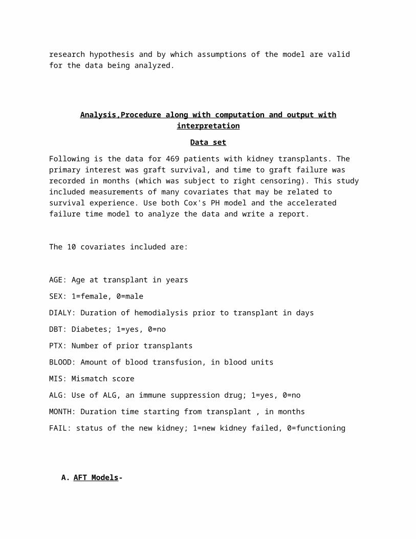
MIS: Mismatch score
ALG: Use of ALG, an immune suppression drug; 1=yes, 0=no
MONTH: Duration time starting from transplant , in months
FAIL: status of the new kidney; 1=new kidney failed, 0=functioning
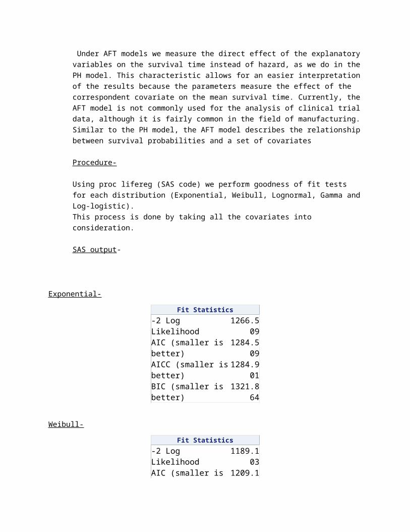
A. AFT Models - Under AFT models we measure the direct effect of the explanatory variables on the survival time instead of hazard, as we do in the PH model. This characteristic allows for an easier interpretation of the results because the parameters measure the effect of the correspondent covariate on the mean survival time. Currently, the AFT model is not commonly used for the analysis of clinical trial data, although it is fairly common in the field of manufacturing. Similar to the PH model, the AFT model describes the relationship between survival probabilities and a set of covariates
Procedure-
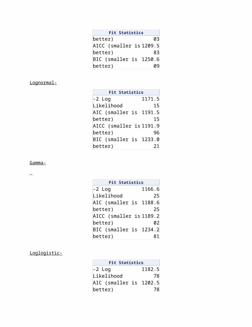
Using proc lifereg (SAS code) we perform goodness of fit tests for each distribution (Exponential, Weibull, Lognormal, Gamma and Log-logistic).This process is done by taking all the covariates into consideration.
SAS output-
Exponential-
Fit Statistics
-2 Log Likelihood1266.50
9
AIC (smaller is better)1284.50
9AICC (smaller is better)
1284.901
BIC (smaller is better)1321.86
4
Weibull-
Fit Statistics
-2 Log Likelihood1189.10
3
Fit Statistics
AIC (smaller is better)1209.10
3AICC (smaller is better)
1209.583
BIC (smaller is better)1250.60
9
Lognormal-
Fit Statistics
-2 Log Likelihood1171.51
5
AIC (smaller is better)1191.51
5AICC (smaller is better)
1191.996
BIC (smaller is better)1233.02
1
Gamma-
Fit Statistics
-2 Log Likelihood1166.62
5
AIC (smaller is better)1188.62
5AICC (smaller is better)
1189.202
BIC (smaller is better)1234.28
1
Loglogistic-
Fit Statistics
-2 Log Likelihood1182.57
8
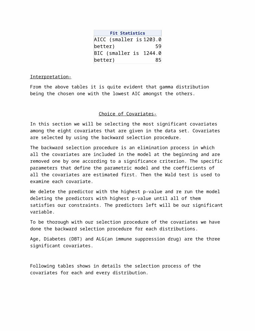
AIC (smaller is better)1202.57
8AICC (smaller is better)
1203.059
BIC (smaller is better)1244.08
5
Interpretation-
From the above tables it is quite evident that gamma distribution being the chosen one with the lowest AIC amongst the others.
Choice of Covariates-
In this section we will be selecting the most significant covariates among the eight covariates that are given in the data set. Covariates are selected by using the backward selection procedure.
The backward selection procedure is an elimination process in which all the covariates are included in the model at the beginning and are removed one by one according to a significance criterion. The specific parameters that define the parametric model and the coefficients of all the covariates are estimated first. Then the Wald test is used to examine each covariate.
We delete the predictor with the highest p-value and re run the model deleting the predictors with highest p-value until all of them satisfies our constraints. The predictors left will be our significant variable.
To be thorough with our selection procedure of the covariates we have done the backward selection procedure for each distributions.
Age, Diabetes (DBT) and ALG(an immune suppression drug) are the three significant covariates.
Following tables shows in details the selection process of the covariates for each and every distribution.
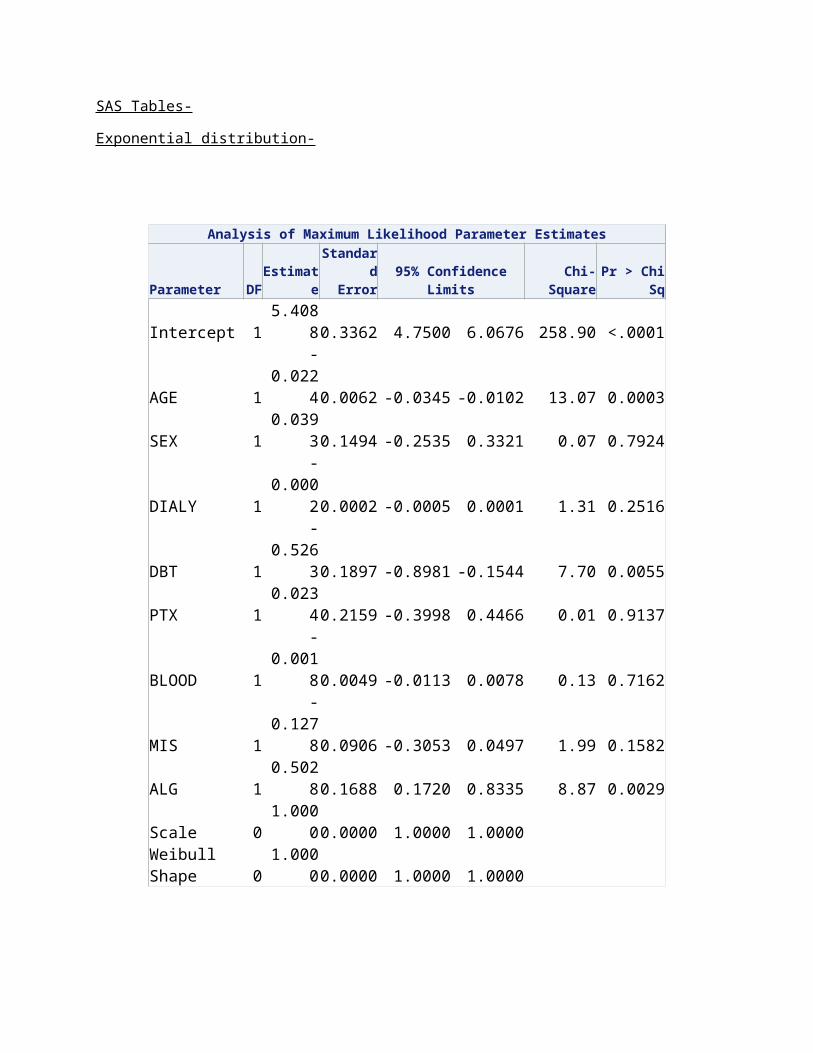
SAS Tables-
Exponential distribution-
Analysis of Maximum Likelihood Parameter Estimates
Parameter DFEstimateStandard
Error95% Confidence LimitsChi-SquarePr > ChiSqIntercept 1 5.4088 0.3362 4.7500 6.0676 258.90 <.0001AGE 1 -0.0224 0.0062 -0.0345 -0.0102 13.07 0.0003SEX 1 0.0393 0.1494 -0.2535 0.3321 0.07 0.7924DIALY 1 -0.0002 0.0002 -0.0005 0.0001 1.31 0.2516DBT 1 -0.5263 0.1897 -0.8981 -0.1544 7.70 0.0055PTX 1 0.0234 0.2159 -0.3998 0.4466 0.01 0.9137BLOOD 1 -0.0018 0.0049 -0.0113 0.0078 0.13 0.7162MIS 1 -0.1278 0.0906 -0.3053 0.0497 1.99 0.1582
Analysis of Maximum Likelihood Parameter Estimates
Parameter DFEstimateStandard
Error95% Confidence LimitsChi-SquarePr > ChiSqALG 1 0.5028 0.1688 0.1720 0.8335 8.87 0.0029Scale 0 1.0000 0.0000 1.0000 1.0000 Weibull Shape 0 1.0000 0.0000 1.0000 1.0000
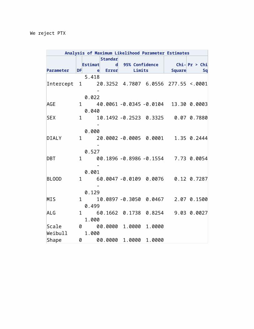
We reject PTX
Analysis of Maximum Likelihood Parameter Estimates
Parameter DFEstimateStandard
Error95% Confidence LimitsChi-SquarePr > ChiSqIntercept 1 5.4182 0.3252 4.7807 6.0556 277.55 <.0001AGE 1 -0.0224 0.0061 -0.0345 -0.0104 13.30 0.0003SEX 1 0.0401 0.1492 -0.2523 0.3325 0.07 0.7880DIALY 1 -0.0002 0.0002 -0.0005 0.0001 1.35 0.2444DBT 1 -0.5270 0.1896 -0.8986 -0.1554 7.73 0.0054BLOOD 1 -0.0016 0.0047 -0.0109 0.0076 0.12 0.7287MIS 1 -0.1291 0.0897 -0.3050 0.0467 2.07 0.1500ALG 1 0.4996 0.1662 0.1738 0.8254 9.03 0.0027Scale 0 1.0000 0.0000 1.0000 1.0000 Weibull Shape 0 1.0000 0.0000 1.0000 1.0000
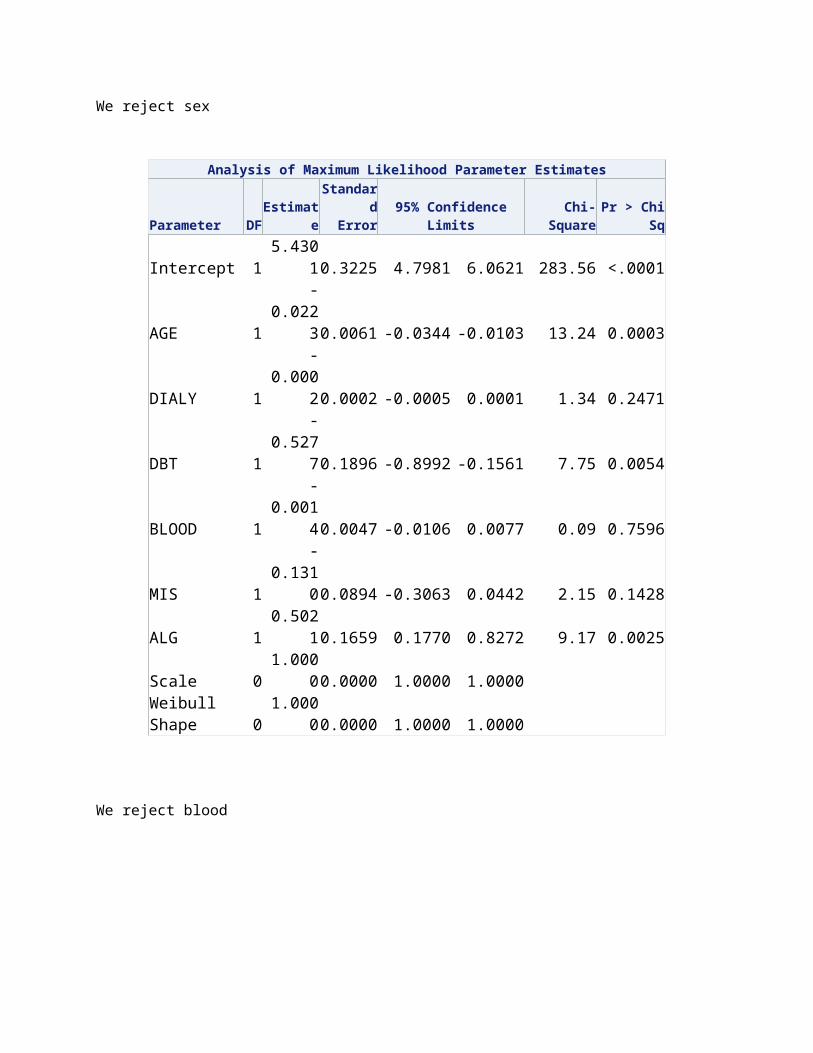
We reject sex
Analysis of Maximum Likelihood Parameter Estimates
Parameter DFEstimateStandard
Error95% Confidence LimitsChi-SquarePr > ChiSqIntercept 1 5.4301 0.3225 4.7981 6.0621 283.56 <.0001AGE 1 -0.0223 0.0061 -0.0344 -0.0103 13.24 0.0003DIALY 1 -0.0002 0.0002 -0.0005 0.0001 1.34 0.2471DBT 1 -0.5277 0.1896 -0.8992 -0.1561 7.75 0.0054BLOOD 1 -0.0014 0.0047 -0.0106 0.0077 0.09 0.7596
Analysis of Maximum Likelihood Parameter Estimates
Parameter DFEstimateStandard
Error95% Confidence LimitsChi-SquarePr > ChiSqMIS 1 -0.1310 0.0894 -0.3063 0.0442 2.15 0.1428ALG 1 0.5021 0.1659 0.1770 0.8272 9.17 0.0025Scale 0 1.0000 0.0000 1.0000 1.0000 Weibull Shape 0 1.0000 0.0000 1.0000 1.0000
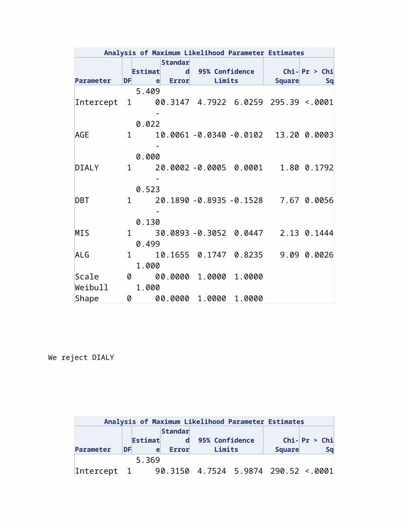
We reject blood
Analysis of Maximum Likelihood Parameter Estimates
Parameter DFEstimateStandard
Error95% Confidence LimitsChi-SquarePr > ChiSqIntercept 1 5.4090 0.3147 4.7922 6.0259 295.39 <.0001AGE 1 -0.0221 0.0061 -0.0340 -0.0102 13.20 0.0003DIALY 1 -0.0002 0.0002 -0.0005 0.0001 1.80 0.1792DBT 1 -0.5232 0.1890 -0.8935 -0.1528 7.67 0.0056MIS 1 -0.1303 0.0893 -0.3052 0.0447 2.13 0.1444ALG 1 0.4991 0.1655 0.1747 0.8235 9.09 0.0026Scale 0 1.0000 0.0000 1.0000 1.0000 Weibull Shape 0 1.0000 0.0000 1.0000 1.0000
We reject DIALY
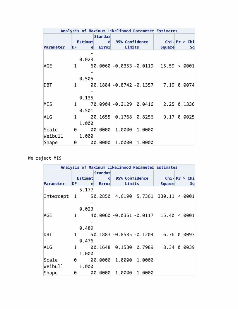
Analysis of Maximum Likelihood Parameter Estimates
Parameter DFEstimateStandard
Error95% Confidence LimitsChi-SquarePr > ChiSqIntercept 1 5.3699 0.3150 4.7524 5.9874 290.52 <.0001AGE 1 -0.0236 0.0060 -0.0353 -0.0119 15.59 <.0001DBT 1 -0.5050 0.1884 -0.8742 -0.1357 7.19 0.0074MIS 1 -0.1357 0.0904 -0.3129 0.0416 2.25 0.1336ALG 1 0.5012 0.1655 0.1768 0.8256 9.17 0.0025Scale 0 1.0000 0.0000 1.0000 1.0000 Weibull 0 1.0000 0.0000 1.0000 1.0000
Analysis of Maximum Likelihood Parameter Estimates
Parameter DFEstimateStandard
Error95% Confidence LimitsChi-SquarePr > ChiSqShape
We reject MIS
Analysis of Maximum Likelihood Parameter Estimates
Parameter DFEstimateStandard
Error95% Confidence LimitsChi-SquarePr > ChiSqIntercept 1 5.1775 0.2850 4.6190 5.7361 330.11 <.0001AGE 1 -0.0234 0.0060 -0.0351 -0.0117 15.40 <.0001DBT 1 -0.4895 0.1883 -0.8585 -0.1204 6.76 0.0093ALG 1 0.4760 0.1648 0.1530 0.7989 8.34 0.0039Scale 0 1.0000 0.0000 1.0000 1.0000 Weibull Shape 0 1.0000 0.0000 1.0000 1.0000
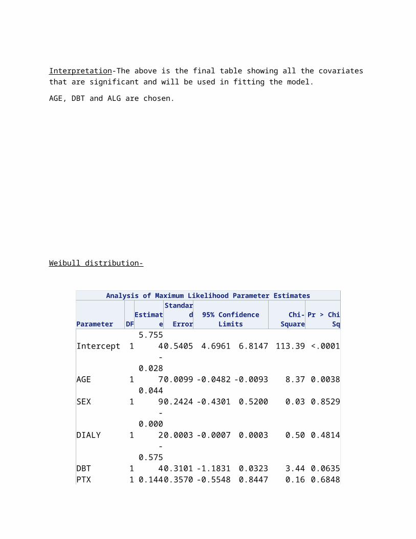
Interpretation-The above is the final table showing all the covariates that are significant and will be used in fitting the model.
AGE, DBT and ALG are chosen.
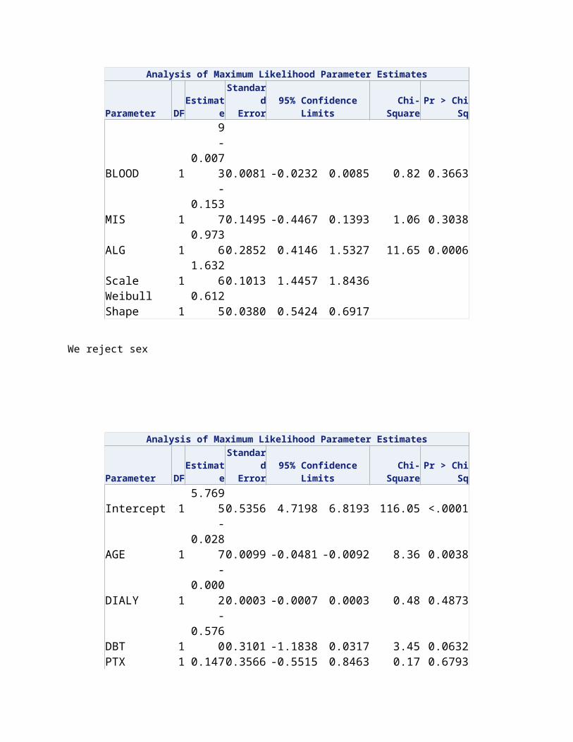
Weibull distribution-
Analysis of Maximum Likelihood Parameter Estimates
Parameter DFEstimateStandard
Error95% Confidence LimitsChi-SquarePr > ChiSqIntercept 1 5.7554 0.5405 4.6961 6.8147 113.39 <.0001AGE 1 -0.0287 0.0099 -0.0482 -0.0093 8.37 0.0038SEX 1 0.0449 0.2424 -0.4301 0.5200 0.03 0.8529
Analysis of Maximum Likelihood Parameter Estimates
Parameter DFEstimateStandard
Error95% Confidence LimitsChi-SquarePr > ChiSqDIALY 1 -0.0002 0.0003 -0.0007 0.0003 0.50 0.4814DBT 1 -0.5754 0.3101 -1.1831 0.0323 3.44 0.0635PTX 1 0.1449 0.3570 -0.5548 0.8447 0.16 0.6848BLOOD 1 -0.0073 0.0081 -0.0232 0.0085 0.82 0.3663MIS 1 -0.1537 0.1495 -0.4467 0.1393 1.06 0.3038ALG 1 0.9736 0.2852 0.4146 1.5327 11.65 0.0006Scale 1 1.6326 0.1013 1.4457 1.8436 Weibull Shape 1 0.6125 0.0380 0.5424 0.6917
We reject sex
Analysis of Maximum Likelihood Parameter Estimates
Parameter DFEstimateStandard
Error95% Confidence LimitsChi-SquarePr > ChiSqIntercept 1 5.7695 0.5356 4.7198 6.8193 116.05 <.0001AGE 1 -0.0287 0.0099 -0.0481 -0.0092 8.36 0.0038DIALY 1 -0.0002 0.0003 -0.0007 0.0003 0.48 0.4873DBT 1 -0.5760 0.3101 -1.1838 0.0317 3.45 0.0632PTX 1 0.1474 0.3566 -0.5515 0.8463 0.17 0.6793BLOOD 1 -0.0071 0.0080 -0.0228 0.0086 0.79 0.3750MIS 1 -0.1551 0.1493 -0.4477 0.1375 1.08 0.2988ALG 1 0.9761 0.2849 0.4177 1.5345 11.74 0.0006Scale 1 1.6327 0.1013 1.4458 1.8438 Weibull Shape 1 0.6125 0.0380 0.5424 0.6917
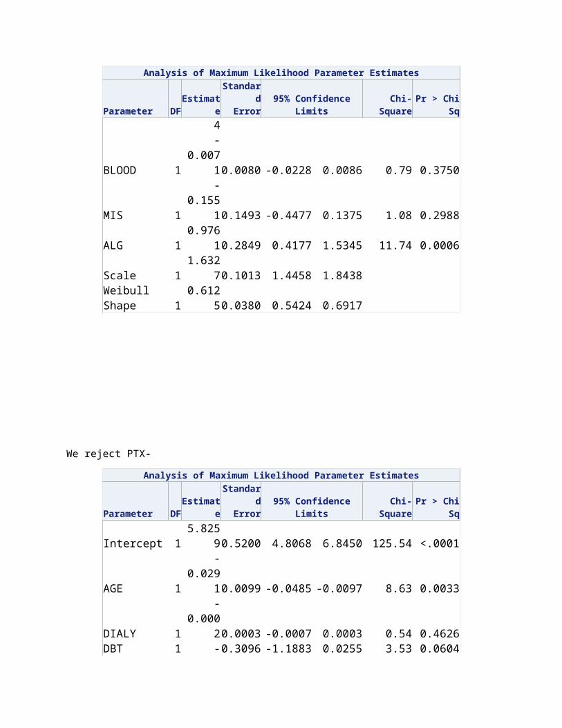
We reject PTX-
Analysis of Maximum Likelihood Parameter Estimates
Parameter DFEstimateStandard
Error95% Confidence LimitsChi-SquarePr > ChiSqIntercept 1 5.8259 0.5200 4.8068 6.8450 125.54 <.0001AGE 1 -0.0291 0.0099 -0.0485 -0.0097 8.63 0.0033DIALY 1 -0.0002 0.0003 -0.0007 0.0003 0.54 0.4626DBT 1 -0.5814 0.3096 -1.1883 0.0255 3.53 0.0604BLOOD 1 -0.0061 0.0077 -0.0213 0.0090 0.63 0.4265MIS 1 -0.1644 0.1476 -0.4537 0.1249 1.24 0.2653ALG 1 0.9553 0.2801 0.4064 1.5042 11.64 0.0006Scale 1 1.6315 0.1011 1.4448 1.8422 Weibull Shape 1 0.6129 0.0380 0.5428 0.6921
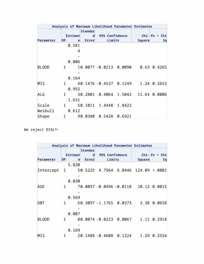
We reject DIALY-
Analysis of Maximum Likelihood Parameter Estimates
Parameter DFEstimateStandard
Error95% Confidence LimitsChi-SquarePr > ChiSqIntercept 1 5.8205 0.5225 4.7964 6.8446 124.09 <.0001AGE 1 -0.0307 0.0097 -0.0496 -0.0118 10.12 0.0015DBT 1 -0.5696 0.3097 -1.1765 0.0373 3.38 0.0658BLOOD 1 -0.0078 0.0074 -0.0223 0.0067 1.11 0.2918MIS 1 -0.1692 0.1488 -0.4608 0.1224 1.29 0.2554ALG 1 0.9634 0.2805 0.4137 1.5132 11.80 0.0006Scale 1 1.6346 0.1013 1.4477 1.8457 Weibull Shape 1 0.6118 0.0379 0.5418 0.6908
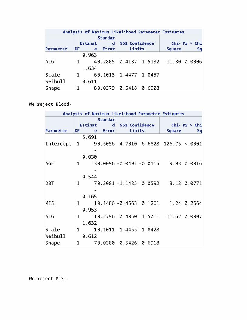
We reject Blood-
Analysis of Maximum Likelihood Parameter Estimates
Parameter DFEstimateStandard
Error95% Confidence LimitsChi-SquarePr > ChiSqIntercept 1 5.6919 0.5056 4.7010 6.6828 126.75 <.0001AGE 1 -0.0303 0.0096 -0.0491 -0.0115 9.93 0.0016DBT 1 -0.5447 0.3081 -1.1485 0.0592 3.13 0.0771MIS 1 -0.1651 0.1486 -0.4563 0.1261 1.24 0.2664ALG 1 0.9531 0.2796 0.4050 1.5011 11.62 0.0007Scale 1 1.6321 0.1011 1.4455 1.8428 Weibull Shape 1 0.6127 0.0380 0.5426 0.6918
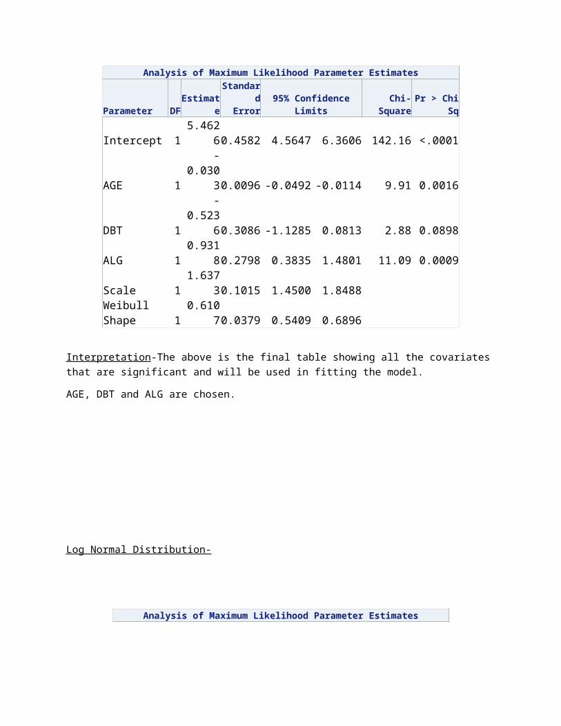
We reject MIS-
Analysis of Maximum Likelihood Parameter Estimates
Parameter DFEstimateStandard
Error95% Confidence LimitsChi-SquarePr > ChiSqIntercept 1 5.4626 0.4582 4.5647 6.3606 142.16 <.0001AGE 1 -0.0303 0.0096 -0.0492 -0.0114 9.91 0.0016DBT 1 -0.5236 0.3086 -1.1285 0.0813 2.88 0.0898ALG 1 0.9318 0.2798 0.3835 1.4801 11.09 0.0009Scale 1 1.6373 0.1015 1.4500 1.8488 Weibull Shape 1 0.6107 0.0379 0.5409 0.6896
Interpretation-The above is the final table showing all the covariates that are significant and will be used in fitting the model.
AGE, DBT and ALG are chosen.
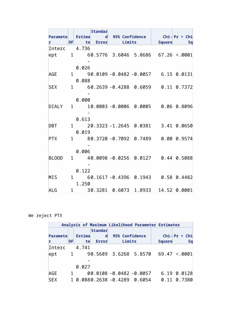
Log Normal Distribution-
Analysis of Maximum Likelihood Parameter Estimates
ParameterDFEstimateStandard
Error95% Confidence LimitsChi-SquarePr > ChiSqIntercept 1 4.7366 0.5776 3.6046 5.8686 67.26 <.0001AGE 1 -0.0269 0.0109 -0.0482 -0.0057 6.15 0.0131SEX 1 0.0886 0.2639 -0.4288 0.6059 0.11 0.7372DIALY 1 -0.0001 0.0003 -0.0006 0.0005 0.06 0.8096DBT 1 -0.6132 0.3323 -1.2645 0.0381 3.41 0.0650PTX 1 0.0198 0.3720 -0.7092 0.7489 0.00 0.9574BLOOD 1 -0.0064 0.0098 -0.0256 0.0127 0.44 0.5088MIS 1 -0.1226 0.1617 -0.4396 0.1943 0.58 0.4482ALG 1 1.2503 0.3281 0.6073 1.8933 14.52 0.0001
We reject PTX
Analysis of Maximum Likelihood Parameter Estimates
ParameterDFEstimateStandard
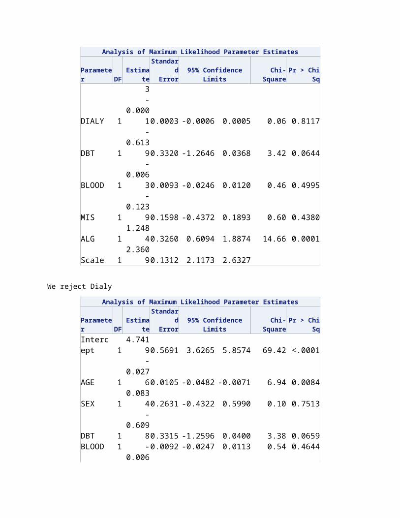
Error95% Confidence LimitsChi-SquarePr > ChiSqIntercept 1 4.7419 0.5689 3.6268 5.8570 69.47 <.0001AGE 1 -0.0270 0.0108 -0.0482 -0.0057 6.19 0.0128SEX 1 0.0883 0.2638 -0.4289 0.6054 0.11 0.7380DIALY 1 -0.0001 0.0003 -0.0006 0.0005 0.06 0.8117DBT 1 -0.6139 0.3320 -1.2646 0.0368 3.42 0.0644BLOOD 1 -0.0063 0.0093 -0.0246 0.0120 0.46 0.4995MIS 1 -0.1239 0.1598 -0.4372 0.1893 0.60 0.4380ALG 1 1.2484 0.3260 0.6094 1.8874 14.66 0.0001Scale 1 2.3609 0.1312 2.1173 2.6327
We reject Dialy
Analysis of Maximum Likelihood Parameter Estimates
ParameterDFEstimateStandard
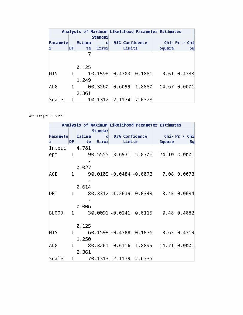
Error95% Confidence LimitsChi-SquarePr > ChiSqIntercept 1 4.7419 0.5691 3.6265 5.8574 69.42 <.0001AGE 1 -0.0276 0.0105 -0.0482 -0.0071 6.94 0.0084SEX 1 0.0834 0.2631 -0.4322 0.5990 0.10 0.7513DBT 1 -0.6098 0.3315 -1.2596 0.0400 3.38 0.0659BLOOD 1 -0.0067 0.0092 -0.0247 0.0113 0.54 0.4644MIS 1 -0.1251 0.1598 -0.4383 0.1881 0.61 0.4338ALG 1 1.2490 0.3260 0.6099 1.8880 14.67 0.0001Scale 1 2.3611 0.1312 2.1174 2.6328
We reject sex
Analysis of Maximum Likelihood Parameter Estimates
ParameterDFEstimateStandard
Error95% Confidence LimitsChi-SquarePr > ChiSqIntercept 1 4.7819 0.5555 3.6931 5.8706 74.10 <.0001AGE 1 -0.0279 0.0105 -0.0484 -0.0073 7.08 0.0078DBT 1 -0.6148 0.3312 -1.2639 0.0343 3.45 0.0634BLOOD 1 -0.0063 0.0091 -0.0241 0.0115 0.48 0.4882MIS 1 -0.1256 0.1598 -0.4388 0.1876 0.62 0.4319ALG 1 1.2508 0.3261 0.6116 1.8899 14.71 0.0001Scale 1 2.3617 0.1313 2.1179 2.6335
We reject blood
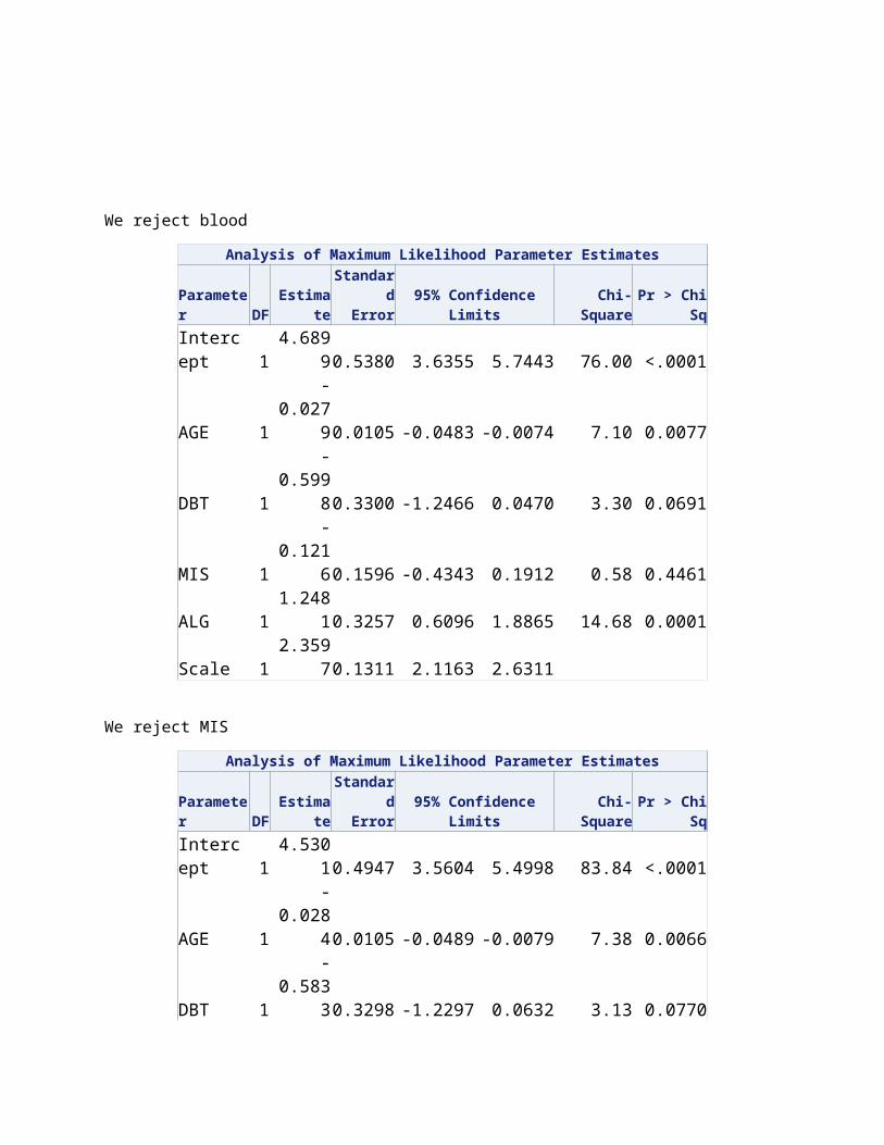
Analysis of Maximum Likelihood Parameter Estimates
ParameterDFEstimateStandard
Error95% Confidence LimitsChi-SquarePr > ChiSqIntercept 1 4.6899 0.5380 3.6355 5.7443 76.00 <.0001AGE 1 -0.0279 0.0105 -0.0483 -0.0074 7.10 0.0077DBT 1 -0.5998 0.3300 -1.2466 0.0470 3.30 0.0691MIS 1 -0.1216 0.1596 -0.4343 0.1912 0.58 0.4461ALG 1 1.2481 0.3257 0.6096 1.8865 14.68 0.0001Scale 1 2.3597 0.1311 2.1163 2.6311
We reject MIS
Analysis of Maximum Likelihood Parameter Estimates
ParameterDFEstimateStandard
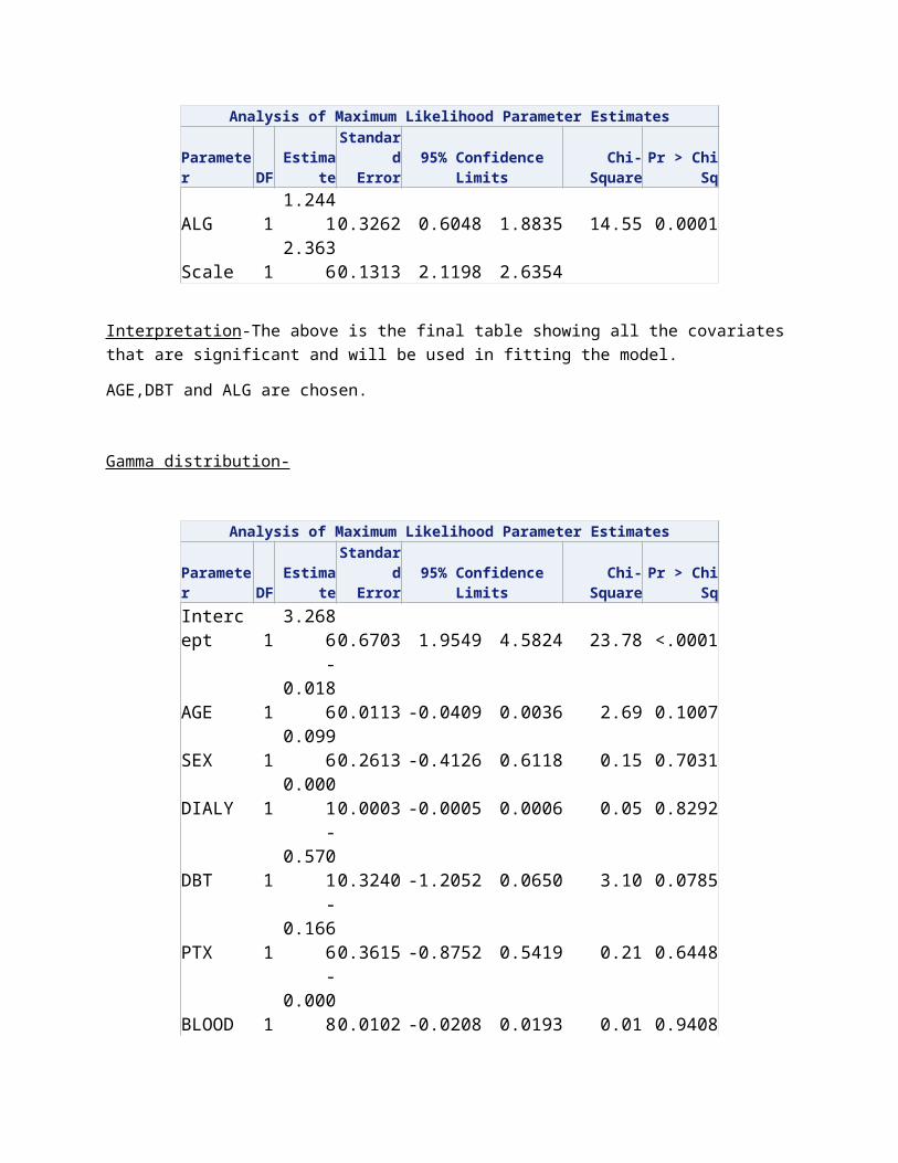
Error95% Confidence LimitsChi-SquarePr > ChiSqIntercept 1 4.5301 0.4947 3.5604 5.4998 83.84 <.0001AGE 1 -0.0284 0.0105 -0.0489 -0.0079 7.38 0.0066DBT 1 -0.5833 0.3298 -1.2297 0.0632 3.13 0.0770ALG 1 1.2441 0.3262 0.6048 1.8835 14.55 0.0001Scale 1 2.3636 0.1313 2.1198 2.6354
Interpretation-The above is the final table showing all the covariates that are significant and will be used in fitting the model.
AGE,DBT and ALG are chosen.
Gamma distribution-
Analysis of Maximum Likelihood Parameter Estimates
ParameterDFEstimateStandard
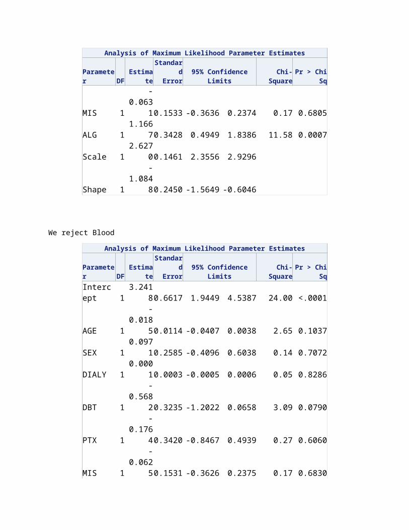
Error95% Confidence LimitsChi-SquarePr > ChiSqIntercept 1 3.2686 0.6703 1.9549 4.5824 23.78 <.0001AGE 1 -0.0186 0.0113 -0.0409 0.0036 2.69 0.1007SEX 1 0.0996 0.2613 -0.4126 0.6118 0.15 0.7031DIALY 1 0.0001 0.0003 -0.0005 0.0006 0.05 0.8292DBT 1 -0.5701 0.3240 -1.2052 0.0650 3.10 0.0785PTX 1 -0.1666 0.3615 -0.8752 0.5419 0.21 0.6448BLOOD 1 -0.0008 0.0102 -0.0208 0.0193 0.01 0.9408MIS 1 -0.0631 0.1533 -0.3636 0.2374 0.17 0.6805ALG 1 1.1667 0.3428 0.4949 1.8386 11.58 0.0007
Analysis of Maximum Likelihood Parameter Estimates
ParameterDFEstimateStandard
Error95% Confidence LimitsChi-SquarePr > ChiSqScale 1 2.6270 0.1461 2.3556 2.9296 Shape 1 -1.0848 0.2450 -1.5649 -0.6046
We reject Blood
Analysis of Maximum Likelihood Parameter Estimates
ParameterDFEstimateStandard
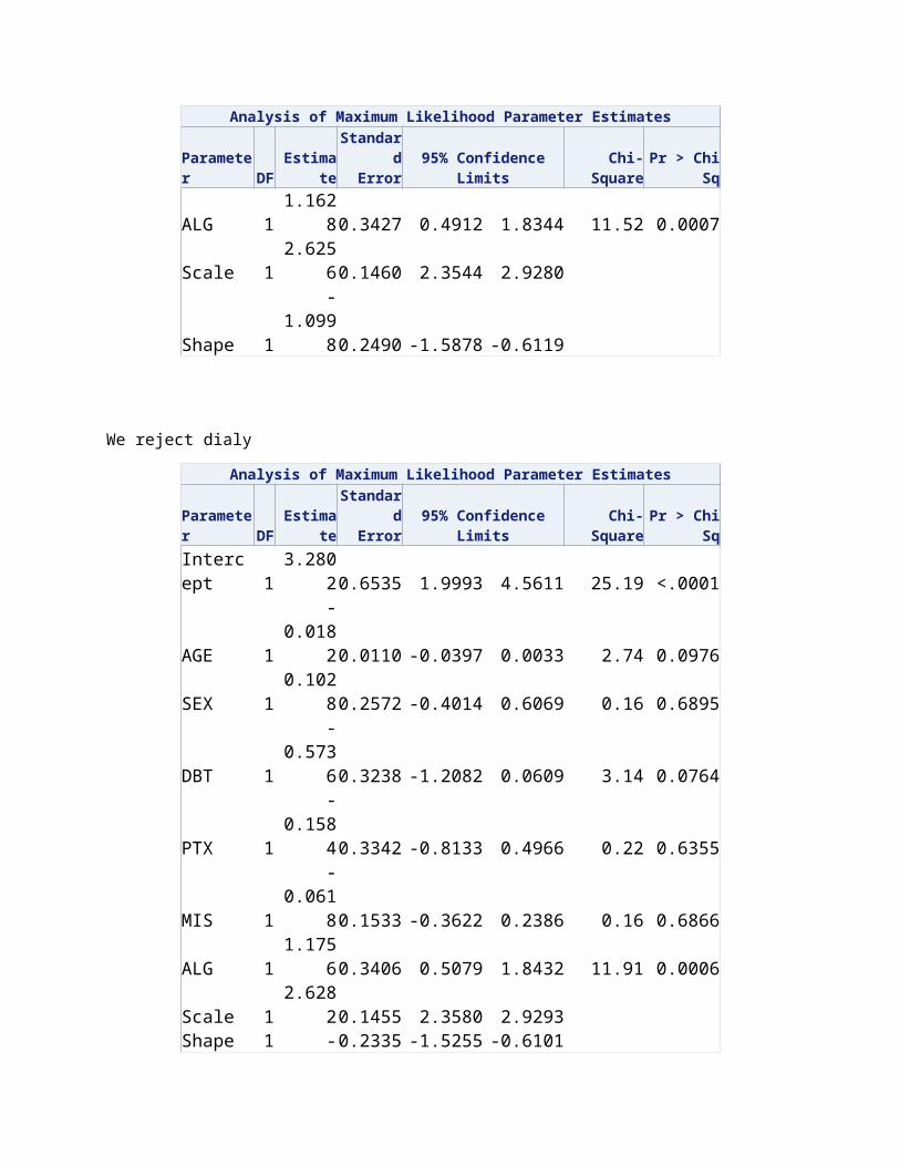
Error95% Confidence LimitsChi-SquarePr > ChiSqIntercept 1 3.2418 0.6617 1.9449 4.5387 24.00 <.0001AGE 1 -0.0185 0.0114 -0.0407 0.0038 2.65 0.1037SEX 1 0.0971 0.2585 -0.4096 0.6038 0.14 0.7072DIALY 1 0.0001 0.0003 -0.0005 0.0006 0.05 0.8286DBT 1 -0.5682 0.3235 -1.2022 0.0658 3.09 0.0790PTX 1 -0.1764 0.3420 -0.8467 0.4939 0.27 0.6060MIS 1 -0.0625 0.1531 -0.3626 0.2375 0.17 0.6830ALG 1 1.1628 0.3427 0.4912 1.8344 11.52 0.0007Scale 1 2.6256 0.1460 2.3544 2.9280 Shape 1 -1.0998 0.2490 -1.5878 -0.6119
We reject dialy
Analysis of Maximum Likelihood Parameter Estimates
ParameterDFEstimateStandard
Error95% Confidence LimitsChi-SquarePr > ChiSqIntercept 1 3.2802 0.6535 1.9993 4.5611 25.19 <.0001AGE 1 -0.0182 0.0110 -0.0397 0.0033 2.74 0.0976SEX 1 0.1028 0.2572 -0.4014 0.6069 0.16 0.6895DBT 1 -0.5736 0.3238 -1.2082 0.0609 3.14 0.0764PTX 1 -0.1584 0.3342 -0.8133 0.4966 0.22 0.6355MIS 1 -0.0618 0.1533 -0.3622 0.2386 0.16 0.6866ALG 1 1.1756 0.3406 0.5079 1.8432 11.91 0.0006Scale 1 2.6282 0.1455 2.3580 2.9293 Shape 1 -1.0678 0.2335 -1.5255 -0.6101
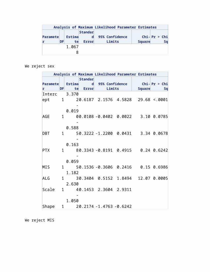
We reject sex
Analysis of Maximum Likelihood Parameter Estimates
ParameterDFEstimateStandard
Error95% Confidence LimitsChi-SquarePr > ChiSqIntercept 1 3.3702 0.6187 2.1576 4.5828 29.68 <.0001AGE 1 -0.0190 0.0108 -0.0402 0.0022 3.10 0.0785
Analysis of Maximum Likelihood Parameter Estimates
ParameterDFEstimateStandard
Error95% Confidence LimitsChi-SquarePr > ChiSqDBT 1 -0.5885 0.3222 -1.2200 0.0431 3.34 0.0678PTX 1 -0.1638 0.3343 -0.8191 0.4915 0.24 0.6242MIS 1 -0.0595 0.1536 -0.3606 0.2416 0.15 0.6986ALG 1 1.1823 0.3404 0.5152 1.8494 12.07 0.0005Scale 1 2.6304 0.1453 2.3604 2.9311 Shape 1 -1.0502 0.2174 -1.4763 -0.6242
We reject MIS
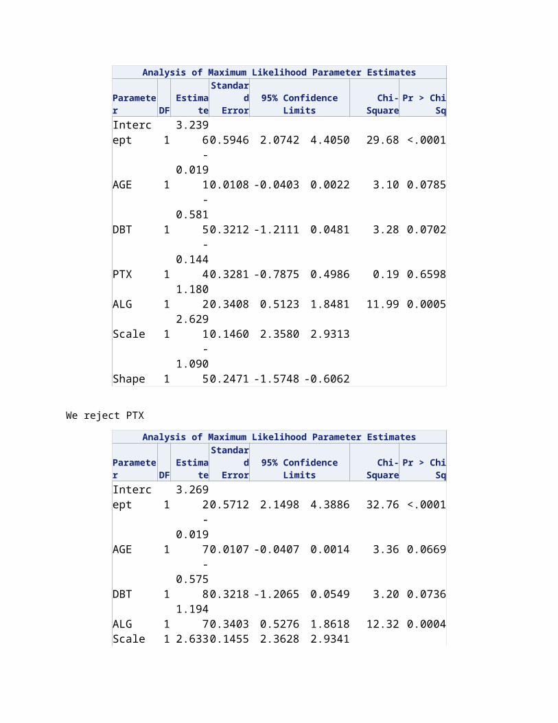
Analysis of Maximum Likelihood Parameter Estimates
ParameterDFEstimateStandard
Error95% Confidence LimitsChi-SquarePr > ChiSqIntercept 1 3.2396 0.5946 2.0742 4.4050 29.68 <.0001AGE 1 -0.0191 0.0108 -0.0403 0.0022 3.10 0.0785DBT 1 -0.5815 0.3212 -1.2111 0.0481 3.28 0.0702PTX 1 -0.1444 0.3281 -0.7875 0.4986 0.19 0.6598ALG 1 1.1802 0.3408 0.5123 1.8481 11.99 0.0005Scale 1 2.6291 0.1460 2.3580 2.9313 Shape 1 -1.0905 0.2471 -1.5748 -0.6062
We reject PTX
Analysis of Maximum Likelihood Parameter Estimates
ParameterDFEstimateStandard
Error95% Confidence LimitsChi-SquarePr > ChiSqIntercept 1 3.2692 0.5712 2.1498 4.3886 32.76 <.0001AGE 1 -0.0197 0.0107 -0.0407 0.0014 3.36 0.0669DBT 1 -0.5758 0.3218 -1.2065 0.0549 3.20 0.0736ALG 1 1.1947 0.3403 0.5276 1.8618 12.32 0.0004Scale 1 2.6330 0.1455 2.3628 2.9341 Shape 1 -1.0523 0.2170 -1.4777 -0.6269
Interpretation-The above is the final table showing all the covariates that are significant and will be used in fitting the model.
AGE,DBT and ALG are chosen.
Log logistic distribution-
Analysis of Maximum Likelihood Parameter Estimates
ParameterDFEstimateStandard
Error95% Confidence LimitsChi-SquarePr > ChiSqIntercept 1 4.8836 0.5809 3.7451 6.0221 70.68 <.0001
Analysis of Maximum Likelihood Parameter Estimates
ParameterDFEstimateStandard
Error95% Confidence LimitsChi-SquarePr > ChiSqAGE 1 -0.0300 0.0108 -0.0512 -0.0089 7.76 0.0053SEX 1 0.1009 0.2663 -0.4210 0.6227 0.14 0.7048DIALY 1 -0.0001 0.0003 -0.0006 0.0005 0.11 0.7400DBT 1 -0.6366 0.3362 -1.2955 0.0224 3.58 0.0583PTX 1 0.0587 0.3906 -0.7069 0.8242 0.02 0.8806BLOOD 1 -0.0085 0.0094 -0.0269 0.0100 0.81 0.3694MIS 1 -0.1580 0.1652 -0.4818 0.1657 0.92 0.3387ALG 1 1.3047 0.3317 0.6545 1.9549 15.47 <.0001Scale 1 1.3746 0.0832 1.2209 1.5476
We reject PTX
Analysis of Maximum Likelihood Parameter Estimates
ParameterDFEstimateStandard
Error95% Confidence LimitsChi-SquarePr > ChiSqIntercept 1 4.9011 0.5690 3.7860 6.0163 74.20 <.0001AGE 1 -0.0302 0.0107 -0.0512 -0.0092 7.92 0.0049SEX 1 0.1018 0.2662 -0.4199 0.6234 0.15 0.7022DIALY 1 -0.0001 0.0003 -0.0006 0.0005 0.11 0.7419DBT 1 -0.6387 0.3359 -1.2970 0.0196 3.62 0.0572BLOOD 1 -0.0080 0.0090 -0.0257 0.0096 0.80 0.3719MIS 1 -0.1611 0.1638 -0.4822 0.1599 0.97 0.3253ALG 1 1.2983 0.3289 0.6537 1.9428 15.58 <.0001Scale 1 1.3744 0.0831 1.2207 1.5473
We reject Dialy
Analysis of Maximum Likelihood Parameter Estimates
ParameterDFEstimateStandard
Error95% Confidence LimitsChi-SquarePr > ChiSqIntercept 1 4.8988 0.5693 3.7829 6.0147 74.04 <.0001AGE 1 -0.0311 0.0104 -0.0514 -0.0108 8.98 0.0027SEX 1 0.0930 0.2649 -0.4262 0.6123 0.12 0.7255DBT 1 -0.6319 0.3353 -1.2890 0.0253 3.55 0.0595BLOOD 1 -0.0085 0.0089 -0.0259 0.0088 0.93 0.3357MIS 1 -0.1635 0.1638 -0.4846 0.1576 1.00 0.3183ALG 1 1.3038 0.3284 0.6602 1.9475 15.76 <.0001Scale 1 1.3748 0.0831 1.2212 1.5478
We reject sex
Analysis of Maximum Likelihood Parameter Estimates
ParameterDFEstimateStandard
Error95% Confidence LimitsChi-SquarePr > ChiSqIntercept 1 4.9432 0.5556 3.8542 6.0321 79.16 <.0001AGE 1 -0.0313 0.0104 -0.0516 -0.0109 9.08 0.0026DBT 1 -0.6363 0.3351 -1.2931 0.0206 3.60 0.0576BLOOD 1 -0.0080 0.0088 -0.0252 0.0091 0.84 0.3582MIS 1 -0.1657 0.1635 -0.4862 0.1548 1.03 0.3110ALG 1 1.3044 0.3285 0.6606 1.9483 15.77 <.0001Scale 1 1.3752 0.0832 1.2215 1.5482
We reject blood
Analysis of Maximum Likelihood Parameter Estimates
ParameterDFEstimateStandard
Error95% Confidence LimitsChi-SquarePr > ChiSqIntercept 1 4.8255 0.5407 3.7658 5.8852 79.66 <.0001AGE 1 -0.0313 0.0104 -0.0516 -0.0109 9.09 0.0026DBT 1 -0.6190 0.3343 -1.2743 0.0362 3.43 0.0641MIS 1 -0.1598 0.1632 -0.4797 0.1601 0.96 0.3275ALG 1 1.2998 0.3283 0.6563 1.9433 15.67 <.0001Scale 1 1.3751 0.0831 1.2215 1.5480
We reject MIS
Analysis of Maximum Likelihood Parameter Estimates
ParameterDFEstimateStandard
Error95% Confidence LimitsChi-SquarePr > ChiSqIntercept 1 4.6074 0.4917 3.6437 5.5711 87.81 <.0001AGE 1 -0.0318 0.0104 -0.0521 -0.0114 9.35 0.0022DBT 1 -0.5949 0.3343 -1.2501 0.0604 3.17 0.0752ALG 1 1.2934 0.3294 0.6477 1.9390 15.41 <.0001Scale 1 1.3795 0.0833 1.2255 1.5528
Interpretation-The above is the final table showing all the covariates that are significant and will be used in fitting the model.
AGE,DBT and ALG are chosen.
Goodness of fit test for the selected covariates and selction of model
In this section we perform the goodness of fit test once again for the three covariates selected in the above section (AGE,DBT and ALG).
We select the Gamma distribution as our appropriate model with the lowest AIC value compared to the others.
Following tables shows the detailed AIC and BIC values for each and every distributions.
SAS output-
Exponential distribution-
Fit Statistics
-2 Log Likelihood1270.64
6
AIC (smaller is better)1278.64
6AICC (smaller is better)
1278.732
BIC (smaller is better)1295.24
9
Weibull distribution-
Fit Statistics
-2 Log Likelihood1192.09
8
AIC (smaller is better)1202.09
8AICC (smaller is better)
1202.227
BIC (smaller is better)1222.85
1
Lognormal distribution-
Fit Statistics
-2 Log Likelihood1172.73
5
AIC (smaller is better)1182.73
5AICC (smaller is better)
1182.865
BIC (smaller is better)1203.48
8
Gamma distribution-
Fit Statistics
-2 Log Likelihood1167.17
1
AIC (smaller is better)1179.17
1AICC (smaller is better)
1179.353
BIC (smaller is better)1204.07
5
Log logistic distribution-
Fit Statistics
-2 Log Likelihood1184.61
5
AIC (smaller is better)1194.61
5AICC (smaller is better)
1194.745
BIC (smaller is better)1215.36
8
Interpretation-Gamma distribution is selected with the lowest AIC value of 1179.171 compared to the others.
Fitting the appropriate model
Gamma AFT model has been selected as the appropriate model for the given data set.
For the gamma distribution we have the following table-
Analysis of Maximum Likelihood Parameter Estimates
ParameterDFEstimateStandard
Error95% Confidence LimitsChi-SquarePr > ChiSqIntercept 1 3.2692 0.5712 2.1498 4.3886 32.76 <.0001AGE 1 -0.0197 0.0107 -0.0407 0.0014 3.36 0.0669DBT 1 -0.5758 0.3218 -1.2065 0.0549 3.20 0.0736ALG 1 1.1947 0.3403 0.5276 1.8618 12.32 0.0004Scale 1 2.6330 0.1455 2.3628 2.9341 Shape 1 -1.0523 0.2170 -1.4777 -0.6269
Hence if T be defined as the survival time we can write the appropriate model as-
Log (Ti)= 3.2692 - .0197(AGE) - .5758(DBT) + 1.1947(ALG) + 2.6330(Error)
B. Cox’s PH Model
The non-parametric method does not control for covariates and it requires categorical predictors. When we have several prognostic variables, we must use multivariate approaches.But we cannot use multiple linear regression or logistic regression because they cannot deal with censored observations. We need another method to model survival data with the presence of censoring. One very popular model in survival data is the Cox proportionalhazards model.
Procedure-
We are going to use proc phreg to estimate the regression coefficient (parameter estimate) based on different methods for ties on the given data.Then we are going to compare those results with the two parametric models, exponential and Weibull for further clarification.
Conclusion-From the test results we can say that the signs of regression coefficient of Age, Duration of hemodialysis (DIALY), Diabetes (DBT), Blood are all positive and thus have a higher hazard risk in the kidney transplants.The coefficients of SEX, PTX (number of prior transplants) and ALG (an immune suppression drug) are all negative indicating low hazard risk in the kidney transplantation.
It is also to be noted that if we compare these value with that of exponential and Weibull they give the opposite results. According to Weibull and exponential-SEX, PTX and ALG have higher hazard risk whereas the Age,DIALY,DBT,Blood and MIS have low hazard risk.
The following SAS tabular values explains our outcome in details.
Breslow-
Analysis of Maximum Likelihood Estimates
ParameterDFParameter
EstimateStandard
ErrorChi-SquarePr > ChiSqHazard
RatioAGE 1 0.01732 0.00611 8.0468 0.0046 1.017SEX 1 -0.02983 0.14882 0.0402 0.8411 0.971
DIALY 10.000093
10.000155
6 0.3581 0.5495 1.000DBT 1 0.35004 0.19236 3.3115 0.0688 1.419PTX 1 -0.07341 0.21763 0.1138 0.7359 0.929BLOOD 1 0.00372 0.00497 0.5592 0.4546 1.004MIS 1 0.08376 0.09196 0.8295 0.3624 1.087ALG 1 -0.60697 0.17033 12.6983 0.0004 0.545
Discrete-
Analysis of Maximum Likelihood Estimates
ParameterDFParameter
EstimateStandard
ErrorChi-SquarePr > ChiSqHazard
RatioAGE 1 0.01776 0.00619 8.2292 0.0041 1.018SEX 1 -0.03055 0.15076 0.0411 0.8394 0.970
DIALY 10.000096
20.000158
3 0.3688 0.5437 1.000DBT 1 0.35882 0.19528 3.3763 0.0661 1.432PTX 1 -0.07548 0.22026 0.1174 0.7318 0.927BLOOD 1 0.00378 0.00503 0.5652 0.4522 1.004MIS 1 0.08623 0.09312 0.8576 0.3544 1.090ALG 1 -0.62313 0.17320 12.9439 0.0003 0.536
Efron-
Analysis of Maximum Likelihood Estimates
ParameterDFParameter
EstimateStandard
ErrorChi-SquarePr > ChiSqHazard
RatioAGE 1 0.01741 0.00610 8.1433 0.0043 1.018SEX 1 -0.03178 0.14888 0.0456 0.8310 0.969
DIALY 10.000090
30.000155
7 0.3364 0.5619 1.000
Analysis of Maximum Likelihood Estimates
ParameterDFParameter
EstimateStandard
ErrorChi-SquarePr > ChiSqHazard
RatioDBT 1 0.35510 0.19234 3.4086 0.0649 1.426PTX 1 -0.07098 0.21839 0.1056 0.7452 0.931BLOOD 1 0.00373 0.00497 0.5617 0.4536 1.004MIS 1 0.08553 0.09205 0.8633 0.3528 1.089ALG 1 -0.61692 0.17051 13.0902 0.0003 0.540
Exact-
Analysis of Maximum Likelihood Estimates
ParameterDFParameter
EstimateStandard
ErrorChi-SquarePr > ChiSqHazard
RatioAGE 1 0.01741 0.00610 8.1440 0.0043 1.018SEX 1 -0.03178 0.14889 0.0456 0.8310 0.969
DIALY 10.000090
30.000155
7 0.3362 0.5620 1.000DBT 1 0.35513 0.19235 3.4086 0.0649 1.426PTX 1 -0.07099 0.21842 0.1056 0.7452 0.931BLOOD 1 0.00373 0.00497 0.5617 0.4536 1.004MIS 1 0.08554 0.09205 0.8636 0.3527 1.089ALG 1 -0.61703 0.17054 13.0913 0.0003 0.540
Parameter models-
Exponential-
Analysis of Maximum Likelihood Parameter Estimates
Parameter DFEstimateStandard
Error95% Confidence LimitsChi-SquarePr > ChiSqIntercept 1 5.4088 0.3362 4.7500 6.0676 258.90 <.0001AGE 1 -0.0224 0.0062 -0.0345 -0.0102 13.07 0.0003SEX 1 0.0393 0.1494 -0.2535 0.3321 0.07 0.7924DIALY 1 -0.0002 0.0002 -0.0005 0.0001 1.31 0.2516DBT 1 -0.5263 0.1897 -0.8981 -0.1544 7.70 0.0055PTX 1 0.0234 0.2159 -0.3998 0.4466 0.01 0.9137BLOOD 1 -0.0018 0.0049 -0.0113 0.0078 0.13 0.7162MIS 1 -0.1278 0.0906 -0.3053 0.0497 1.99 0.1582ALG 1 0.5028 0.1688 0.1720 0.8335 8.87 0.0029Scale 0 1.0000 0.0000 1.0000 1.0000 Weibull Shape 0 1.0000 0.0000 1.0000 1.0000
Weibull-
Analysis of Maximum Likelihood Parameter Estimates
Parameter DFEstimateStandard
Error95% Confidence LimitsChi-SquarePr > ChiSqIntercept 1 5.7554 0.5405 4.6961 6.8147 113.39 <.0001AGE 1 -0.0287 0.0099 -0.0482 -0.0093 8.37 0.0038SEX 1 0.0449 0.2424 -0.4301 0.5200 0.03 0.8529DIALY 1 -0.0002 0.0003 -0.0007 0.0003 0.50 0.4814DBT 1 -0.5754 0.3101 -1.1831 0.0323 3.44 0.0635PTX 1 0.1449 0.3570 -0.5548 0.8447 0.16 0.6848BLOOD 1 -0.0073 0.0081 -0.0232 0.0085 0.82 0.3663MIS 1 -0.1537 0.1495 -0.4467 0.1393 1.06 0.3038ALG 1 0.9736 0.2852 0.4146 1.5327 11.65 0.0006Scale 1 1.6326 0.1013 1.4457 1.8436 Weibull Shape 1 0.6125 0.0380 0.5424 0.6917
Choice of Covariates
Like we did in the AFT model in this section we will be selecting the significant covariates only, using Breslow’s method (default procedure) for ties, the backward selection method, and the SAS proc phreg.
Conclusion- AGE, DBT and ALG are the three covariates that are significant from our test results.
Following SAS tables give us the detailed process of the backward selection procedure.
Using Breslow approximation of ties and backward selection-
Analysis of Maximum Likelihood Estimates
ParameterDFParameter
EstimateStandard
ErrorChi-SquarePr > ChiSqHazard
RatioAGE 1 0.01732 0.00611 8.0468 0.0046 1.017SEX 1 -0.02983 0.14882 0.0402 0.8411 0.971
DIALY 10.000093
10.000155
6 0.3581 0.5495 1.000DBT 1 0.35004 0.19236 3.3115 0.0688 1.419PTX 1 -0.07341 0.21763 0.1138 0.7359 0.929BLOOD 1 0.00372 0.00497 0.5592 0.4546 1.004MIS 1 0.08376 0.09196 0.8295 0.3624 1.087ALG 1 -0.60697 0.17033 12.6983 0.0004 0.545
We reject sex-
Analysis of Maximum Likelihood Estimates
ParameterDFParameter
EstimateStandard
ErrorChi-SquarePr > ChiSqHazard
RatioAGE 1 0.01731 0.00611 8.0406 0.0046 1.017
DIALY 10.000091
00.000155
1 0.3441 0.5574 1.000DBT 1 0.35031 0.19234 3.3171 0.0686 1.420PTX 1 -0.07537 0.21728 0.1203 0.7287 0.927BLOOD 1 0.00359 0.00493 0.5305 0.4664 1.004MIS 1 0.08476 0.09181 0.8524 0.3559 1.088ALG 1 -0.60890 0.17001 12.8275 0.0003 0.544
We reject PTX-
Analysis of Maximum Likelihood Estimates
ParameterDFParameter
EstimateStandard
ErrorChi-SquarePr > ChiSqHazard
RatioAGE 1 0.01753 0.00609 8.2854 0.0040 1.018
Analysis of Maximum Likelihood Estimates
ParameterDFParameter
EstimateStandard
ErrorChi-SquarePr > ChiSqHazard
Ratio
DIALY 10.000095
00.000154
2 0.3799 0.5376 1.000DBT 1 0.35394 0.19211 3.3945 0.0654 1.425BLOOD 1 0.00309 0.00475 0.4232 0.5154 1.003MIS 1 0.08957 0.09078 0.9735 0.3238 1.094ALG 1 -0.59912 0.16774 12.7568 0.0004 0.549
We reject Dialy-
Analysis of Maximum Likelihood Estimates
ParameterDFParameter
EstimateStandard
ErrorChi-SquarePr > ChiSqHazard
RatioAGE 1 0.01835 0.00593 9.5785 0.0020 1.019DBT 1 0.34675 0.19167 3.2728 0.0704 1.414BLOOD 1 0.00393 0.00454 0.7474 0.3873 1.004MIS 1 0.09187 0.09122 1.0142 0.3139 1.096ALG 1 -0.60177 0.16772 12.8728 0.0003 0.548
We reject blood-
Analysis of Maximum Likelihood Estimates
ParameterDFParameter
EstimateStandard
ErrorChi-SquarePr > ChiSqHazard
RatioAGE 1 0.01824 0.00592 9.4984 0.0021 1.018DBT 1 0.33636 0.19123 3.0940 0.0786 1.400MIS 1 0.09052 0.09121 0.9848 0.3210 1.095ALG 1 -0.59750 0.16753 12.7202 0.0004 0.550
We reject MIS-
Analysis of Maximum Likelihood Estimates
ParameterDFParameter
EstimateStandard
ErrorChi-SquarePr > ChiSqHazard
RatioAGE 1 0.01827 0.00591 9.5362 0.0020 1.018DBT 1 0.32304 0.19083 2.8656 0.0905 1.381ALG 1 -0.58475 0.16708 12.2492 0.0005 0.557
This is the table for final model with significant covariates.
Fitting of the Model
Analysis of Maximum Likelihood Estimates
ParameterDFParameter
EstimateStandard
ErrorChi-SquarePr > ChiSqHazard
RatioAGE 1 0.01827 0.00591 9.5362 0.0020 1.018DBT 1 0.32304 0.19083 2.8656 0.0905 1.381ALG 1 -0.58475 0.16708 12.2492 0.0005 0.557
Form the above table we can get our significant covariates and hence we can construct our final model
The final model with significant (p<.10) covariates is-
Log[h(t)/ho(t)]=.01827 AGE + .32304 DBT - .58475 ALG
Interpretation- The positive sign of the regression coefficient of AGE and DBT implies high hazard risk rate in kidney transplant whereas the negative coefficient of ALG drug implies low hazard risk rate.