Survey of Maneuvering Target Tracking. Part I: … · applicability of a target dynamic model for a...

Survey of ManeuveringTarget Tracking.Part I: Dynamic Models

X. RONG LI, Senior Member, IEEE

VESSELIN P. JILKOV, Member, IEEEUniversity of New Orleans

This is the first part of a comprehensive and up-to-date survey

of the techniques for tracking maneuvering targets without

addressing the so-called measurement-origin uncertainty. It

surveys various mathematical models of target motion/dynamics

proposed for maneuvering target tracking, including 2D and 3D

maneuver models as well as coordinate-uncoupled generic models

for target motion. This survey emphasizes the underlying ideas

and assumptions of the models. Interrelationships among models

and insight to the pros and cons of models are provided. Some

material presented here has not appeared elsewhere.

CONTENTS

I. Introduction

II. Mathematical Models for Maneuvering Target Tracking

III. Nonmaneuver Models

IV. Coordinate-Uncoupled Maneuver Models

V. 2D Horizontal Motion Models

VI. 3D Motion Models

VII. Concluding Remarks

References

Manuscript received September 11, 2002; revised April 22, 2003;released for publication July 31, 2003.

IEEE Log No. T-AES/39/4/822061.

Refereeing of this contribution was handled by P. K. Willett.

This research was supported in part by ONR GrantN00014-00-1-0677, NSF Grant ECS-9734285, and NASA/LEQSFGrant (2001-4)-01.

Authors’ address: Dept. of Electrical Engineering, University ofNew Orleans, New Orleans, LA 70148, E-mail: ([email protected]).

0018-9251/03/$17.00 c 2003 IEEE

I. INTRODUCTION

The key to successful target tracking lies in theeffective extraction of useful information about thetarget’s state from observations. A good model ofthe target will certainly facilitate this informationextraction to a great extent. In general, one can saywithout exaggeration that a good model is worth athousand pieces of data. This statement has an evenstronger positive connotation in target tracking whereobservation data are rather limited. Most trackingalgorithms are model based because knowledge oftarget motion is available and a good model-basedtracking algorithm will greatly outperform anymodel-free tracking algorithm if the underlying modelturns out to be a good one. As such, it is hard tooverstate the importance of the role of a good modelhere.

Various mathematical models of target motionhave been developed over the past three decades.They are, however, scattered in the literature. Manyof them have never appeared in any periodical in thepublic domain. As a result, few people have a goodknowledge of these models. This is partly due to alack of a comprehensive survey. The importance ofsuch a survey for both practitioners and researchersin the tracking community is evident. The single bestsource so far is, in our opinion, the recent book byBlackman and Popoli [1], which is nonetheless farfrom complete. Some more or less standard modelsfor target motion can be found in established bookson target tracking and/or estimation, such as [2–12].

This paper is the first part of a comprehensive andup-to-date survey of the techniques for maneuveringtarget tracking. The survey is an ongoing project.The conference versions of its first several partshave appeared in [13–17]. It is well known that theso-called measurement-origin uncertainty and targetmotion uncertainty are two major challenges in targettracking. To limit the scope of the work, this surveydeals only with the second uncertainty, leaving thetechniques unique for the data-association problemsuntouched.

Target detection, tracking, and recognition areclosely interrelated areas, with significant overlaps.It is not easy to draw a clear line to separate them. Tobe relatively more focused, this part covers mainlydynamic models of a “point target,” that is, thoseof the dynamic (temporal) behaviors, rather thanspatial characteristics, of a target. While many ofthese models are also useful for target detection andrecognition, this survey is only concerned with theirvalue for target tracking. This of course does notprevent us from developing or applying a model thatdescribes both the temporal evolution and spatialcharacteristics of a target.

Needless to say, target dynamic modelsand tracking algorithms have intimate ties. The

IEEE TRANSACTIONS ON AEROSPACE AND ELECTRONIC SYSTEMS VOL. 39, NO. 4 OCTOBER 2003 1333

applicability of a target dynamic model for a practicalproblem can hardly be evaluated without referring tothe corresponding tracking algorithms used. In otherwords, some target models and tracking algorithmswork well jointly. To be more focused and concise,however, this interdependence is largely ignoredhere.This survey emphasizes the underlying ideas

and assumptions of the models. This should helpthe reader understand not only how these modelswork but also their pros and cons. It is hoped thata distinctive feature of this survey is that it revealswell the interrelationships among various models.However, the reader should keep in mind that muchof such discussion is based on our personal views andpreferences, not always accurate or unbiased, althougha great deal of effort has been made toward thisgoal. In addition to such discussions, some materialincluded in this survey has not appeared elsewhere.Regrettably, many important issues associated

with the target dynamic models, particularly thoseof implementation, cannot be discussed (at least toa desirable degree) due to space limitation as wellas our background and experience. Nevertheless, wewould appreciate very much receiving comments andany missing material that should be covered in thissurvey.This paper is a heavily revised and extended

version of [13]. Its remaining part is organizedas follows. Section II gives briefly state-spacerepresentations of target dynamics and observationsystem. Section III describes nonmaneuver models.The presentation of dynamic models of targetmaneuvers breaks down as follows: while Section IVdeals with those that are uncoupled along differentspatial coordinates, 2D and 3D coupled models arereviewed in Sections V and VI, respectively. The finalsection provides concluding remarks.

II. MATHEMATICAL MODELS FOR MANEUVERINGTARGET TRACKING

The primary objective of target tracking is toestimate the state trajectories of a target—a movingor movable object. Although a target is almost neverreally a point in space and the information aboutits orientation is valuable for tracking, a target isusually treated as a point object without a shape intracking, especially in target dynamic models. A targetdynamic/motion model describes the evolution of thetarget state with respect to time.Almost all maneuvering target tracking methods

are model based. They assume that the target motionand its observations can be represented by someknown mathematical models sufficiently accurately.The most commonly used such models are thoseknown as state-space models, in the following form

of additive noise,

xk+1 = fk(xk,uk) +wk (1)

zk = hk(xk) + vk (2)

where xk, zk, and uk are the target state, observation,and control input vectors, respectively, at the discretetime tk; wk and vk are process and measurementnoise sequences, respectively; and fk and hk are somevector-valued (possibly time-varying) functions. Sucha discrete-time model is often obtained1 by discretizing(sampling) the following continuous-time model [2]2

_x(t) = f(x(t),u(t), t) +w(t), x(t0) = x0 (3)

z(t) = h(x(t), t)+ v(t) (4)

where xk = x(tk) and it is usually assumed3 that

zk = z(tk),vk = v(tk),hk(xk) = h(x(tk), tk). The controlinput is often assumed (approximately) piecewiseconstant with uk = u(t), tk t < tk+1 when discretizinga continuous-time system. In target tracking, thecontrol input u is usually not known. Note that

wk = w(tk), fk(xk,uk ,wk) = f(x(tk),u(tk),w(tk), tk):

In fact, it is often more appropriate to use thefollowing mixed-time models for most trackingproblems

_x(t) = f(x(t),u(t), t) +w(t), x(t0) = x0 (5)

zk = hk(xk) + vk (6)

because while observations are usually availableonly at discrete time instants, the target motion ismore accurately modeled in continuous time. Forexample, target motions should not depend on howand when samples are taken, which is often the case,however, for a discrete-time model. For a similarreason, a discrete-time equivalent model is usually

1One so obtained is referred to as a discretized model regardlessof its equivalence to the continuous-time system. It is termeda discrete-time equivalent if the discretization is exact and theeffects of the continuous-time and discrete-time noise processes areequivalent, which is the case for a linear system without the controlinput u with the standard discretization (i.e., sample and hold).Note, however, that not all discrete-time models can be obtainedby discretizing a continuous-time system. A model defined directlyin discrete time following the same principle as one in continuoustime is referred to as a direct discrete-time counterpart here. We usethe term discrete-time version for either or both of discretized anddirect discrete-time models.2We sacrifice rigor for readability: (3) is not actually well definedbecause _x= dx=dt may not exist at all since the “continuous-timewhite noise” has infinite variance and is a specter in the cosmosthat represents the nonexistent derivative of a Wiener process andthe like. We warn, however, that formal manipulation of (3) or (8)may easily lead to incorrect results. That is why in the mathematicalworld (3) is replaced by dx(t) = f(x(t),u(t), t)dt+ dw(t), x(t0) = x0and certain rules must be followed.3Although discrete-time measurement zk and thus the function hkand noise vk are in fact from sensors that do integration over time.

1334 IEEE TRANSACTIONS ON AEROSPACE AND ELECTRONIC SYSTEMS VOL. 39, NO. 4 OCTOBER 2003

more systematic and consistent, and is in manycases probably preferable to the corresponding directdiscrete-time counterpart.The continuous-, discrete-, and mixed-time

linear counterparts of the above models are thecorresponding pairs of the following equations

xk+1 = Fkxk +Ekuk +Gkwk (7)

_x(t) = A(t)x(t) +E(t)u(t) +B(t)w(t), x(t0) = x0

(8)

zk =Hkxk + vk (9)

z(t) = C(t)x(t) + v(t): (10)

One of the major challenges for target trackingarises from the target motion uncertainty. Thisuncertainty refers to the fact that an accurate dynamicmodel of the target being tracked is not availableto the tracker. Specifically, although the generalform of the model (1) or (5) is usually adequate,a tracker lacks knowledge about the actual controlinput u of the target, and possibly the actual formof f, its parameters, or statistical properties of thenoise w for the particular target being tracked. Targetmotion modeling is thus one of the first tasks formaneuvering target tracking. It aims at developing atractable model that accounts well for the effect oftarget motion.In this paper, we describe the efforts and

results in modeling the target motion for tracking amaneuvering target without knowing its true dynamicbehavior. Most of these efforts have been made alongtwo lines: 1) approximate the actually nonrandomcontrol input u as a random process of certainproperties, and 2) describe typical target trajectoriesby some representative motion models with properlydesigned parameters.Target motions are normally classified into

two classes: maneuver and nonmaneuver. Anonmaneuvering motion is the straight and levelmotion at a constant velocity4 in an inertial referencesystem, sometimes also referred to as the uniformmotion. Loosely speaking, all other motions belongto the maneuvering mode.

III. NONMANEUVER MODELS

It is well known that a point moving in our3D physical world can be described by its 3Dposition and velocity vectors. For instance,5 x=[x, _x,y, _y,z, _z] can be used as a state vector of sucha point in the Cartesian coordinate system, where(x,y,z) are the position coordinates along x, y, and

4Note that velocity is a vector and speed is its magnitude.5In this survey, the regular symbol x and z are used for simplicityto denote the state and measurement vectors, respectively, while thepositions along the x, y, and z axes are denoted by sans serif font(x,y,z).

z axes, respectively, and [ _x, _y, _z] is the velocityvector. When a target is treated as a point object,the nonmaneuvering motion is thus described by thevector-valued equation _x(t) = 0, where x= [_x, _y,z] .Note that z direction is treated differently because anonmaneuvering motion is assumed in the horizontalx–y plane. In practice, this ideal equation is usuallymodified as _x(t) = w(t) 0, where w(t) is whitenoise with a “small” effect on x that accounts forunpredictable modeling errors due to turbulence, etc.The corresponding state-space model is given by, withstate vector x= [x, _x,y, _y,z] ,

_x(t) = diag[Acv,0]x(t) +diag[Bcv,1]w(t) (11)

where w(t) = [wx(t),wy(t),wz(t)] is a continuous-timevector-valued white noise process with power spectraldensity matrix diag[Sx,Sy,Sz], Acv = diag[A2,A2], andBcv = diag[B2,B2] with

6

A2 =0 1

0 0, B2 =

0

1: (12)

The direct discrete-time counterpart of the abovemodel is [2]

xk+1 = Fxk +Gwk = diag[Fcv,1]xk +diag[Gcv,T]wk

= diag[F2,F2,1]xk +diag[G2,G2,T]wk (13)

where

Fcv = diag[F2,F2], Gcv = diag[G2,G2]

F2 =1 T

0 1, G2 =

T2=2

T

(14)

wk = [wx,wy,wz]k is a discrete-time white noisesequence and T is the sampling interval. Note thatwx and wy correspond to noisy “accelerations” alongx and y axes, respectively, while wz corresponds tonoisy “velocity” along z axis. If w is uncoupled acrossits components, then the nonmaneuvering motionmodeled by the above models is uncoupled across x,y, and z directions. In this case, the covariance of thenoise term in (13) is given by

cov(Gwk) = diag[var(wx)Q2,var(wy)Q2,var(wz)]

Q2 =T4=4 T3=2

T3=2 T2:

(15)

This model is defined directly in discrete time and isnot entirely equivalent to the above continuous-timemodel.

The discrete-time equivalent of the abovecontinuous-time model is [2]

xk+1 = diag[F2,F2,1]xk +wk (16)

6For convenience, we use the shorthand notation A=diag[A1,A2, : : : ,An] to denote a block-diagonal matrix A, where Aiand A are not necessarily square matrices.

LI & JILKOV: SURVEY OF MANEUVERING TARGET TRACKING. PART I: DYNAMIC MODELS 1335

where

cov(wk) = diagSxTQ2,

SyTQ2,

SzT

Q2 =T4=3 T3=2

T3=2 T2:

(17)

Note the difference between the discrete-timeequivalent (16) and the direct discrete-time counterpart(13).In a 2D scenario where the altitude z is not

considered, the above models take the more popularform, respectively,

_x(t) = Acvx(t) +Bcvw(t)

xk+1 = Fcvxk +Gcvwk

xk+1 = Fcvxk +wk:

(18)

The above models (11), (13), (16), and (18)are known as the continuous- and discrete-timeconstant-velocity (CV) models, or more precisely,“nearly-constant-velocity models.” Equation (18)is in fact a “(small) white acceleration model”since accelerations along x and y directions aremodeled as (small) white noise. The term “(nearly)constant-velocity model” emphasizes that theseaccelerations are small. Note that the control inputu is zero in the nonmaneuver models, although inreality an actual thrust of the target may be presentto balance other forces so as to maintain the motion.Also, inclusion of any unnecessary component(e.g., acceleration) in the state vector would degradetracking performance.

IV. COORDINATE-UNCOUPLED MANEUVERMODELS

The control input u responsible for a targetmaneuver is primarily deterministic in nature andmost often unknown to the tracker. A natural wayis to model it as an unknown, deterministic processand estimate this process from measurement dataduring tracking. Such deterministic input models arethe basis for the so-called input estimation method(see, e.g., [16, 18–25]). Due to a lack of knowledge ofits dynamics, this unknown process is often assumedto be piecewise constant and treated as an unknowntime-invariant parameter over a time window. Themain difficulty then lies in the determination of theinput level and the instants at which the input jumps.This method is covered in detail in a subsequent partof this survey, of which [16] is a preliminary version.An alternative is to model the input u as a random

process, which is in fact much more popular than theabove deterministic modeling. Models in this classproposed in the literature can be largely classified intothree groups as follows.1) White noise models: The control

input is modeled as white noise. This includes

constant-velocity, constant-acceleration, andpolynomial models.

2) Markov process models: The control inputis modeled as a Markov process, which has a timeautocorrelation. This includes the well-known Singermodel, its various extensions, and some othermodels.

3) Semi-Markov jump process models: Thecontrol input is modeled as a semi-Markov jumpprocess.

Most target maneuvers are coupled across differentcoordinates. For simplicity, however, many maneuvermodels developed assume that this coordinatecoupling is weak and can be neglected. This isparticularly the case for those that model the controlinput u as a random process. As a consequence, weneed to consider only a generic coordinate direction.

Let x, _x, and x be the target position, velocity, andacceleration along a generic direction, respectively.Specifically,

x(t) = a(t): (19)

The models discussed in this section differ in how thefunction a(t) is defined.

In this section, the state vector is always takento be x= [x, _x, x] along the generic direction, unlessstated otherwise explicitly.

A. White-Noise Acceleration Model

The simplest model for a target maneuveris the so-called white-noise acceleration model[2]. It assumes that the target acceleration x(t) isan independent process (strictly white noise). Itdiffers from the nonmaneuver model of SectionIII only in the noise level: the white noise processw used to model the effect of the control input uhas a much higher intensity than the one used in anonmaneuver model. A maneuver by its very natureaims at accomplishing a certain task and thus israrely independent with respect to time. The mainattractive feature of this model is its simplicity. It issometimes used when the maneuver is quite small orrandom. It is also used in some maneuvering targettracking techniques, such as the so-called noise-leveladjustment, discussed in a subsequent part of thissurvey (see [16] for a preliminary version).

B. Wiener-Process Acceleration Model

The second simplest model is the so-calledWiener-process acceleration model [2]. It assumesthat the acceleration is a Wiener process, or moregenerally and precisely, the acceleration is a processwith independent increments, which is not necessarilya Wiener process. It is also referred to simply as theconstant-acceleration (CA) model or more precisely“nearly-constant-acceleration model.”


This model has two commonly used versions. Thefirst one, referred to as the white-noise jerk model,assumes that the acceleration derivative (i.e., “jerk”)_a(t) is an independent process (white noise) w(t):_a(t) = w(t), with power spectral density Sw. Thecorresponding state-space representation is _x(t) =A3x(t) +B3w(t), where

A3 =

0 1 0

0 0 1

0 0 0

, B3 =

0

0

1

: (20)

Its discrete-time equivalent is

xk+1 = F3xk +wk, F3 =

1 T T2=2

0 1 T

0 0 1

(21)

where

Q = cov(wk) = SwQ3, Q3 =

T5=20 T4=8 T3=6

T4=8 T3=3 T2=2

T3=6 T2=2 T

:

(22)

Note that Sw is the power spectral density, not thevariance, of the continuous-time white noise w(t).The second version can be called Wiener-sequence

acceleration model. It assumes that the accelerationincrement is an independent (white noise) process.An acceleration increment over a time period is theintegral of the jerk over the period. This model ismost conveniently expressed in discrete time directly,given by

xk+1 = F3xk +G3wk, G3 =

T2=2

T

1

: (23)

Note that its noise term has a covariance differentfrom that of the white-noise jerk model:

Q = cov(G3wk) = var(wk)

T4=4 T3=2 T2=2

T3=2 T2=2 T

T2=2 T 1

:

(24)

The above models are simple but crude. Actualmaneuvers seldom have (nearly) constant accelerationsthat are uncoupled across coordinate directions.As explained before, a continuous-time model is

more accurate than its discrete-time versions for mostpractical situations since a target moves continuouslyover time. The assumption of the direct discrete-timeCA model (i.e., the second version above) that theacceleration increment ¢ak = ak+1 ak = a(tk+1) a(tk)is independent across different sampling intervalsis hardly justifiable, except for its simplicity andmathematical tractability. Were this assumption true

for a sampling period T, it would not be true ingeneral for any other sampling period T unless it isa multiple of T: T = nT. Even if such periods exist,we would not be so lucky that one of them is used bychance.

C. Polynomial Models

It is well known that any continuous targettrajectory can be approximated by a polynomial ofa certain degree to an arbitrary accuracy. As such, itis possible to model target motion by an nth-degreepolynomial [2] in the Cartesian coordinates:

x(t)

y(t)

z(t)

=

a0 a1 an

b0 b1 bn

c0 c1 cn

1

t...

tn=n!

+

wx(t)

wy(t)

wz(t)

(25)

with a certain choice of the coefficients ai,bi,ci, where(x,y,z) are the position coordinates and (wx,wy,wz)are the corresponding noise terms. Such an nth-degreepolynomial model amounts to assuming the nth timederivative of the position is (nearly) constant (i.e., theposition deviation from such a constant nth derivativemotion is equal to the noise w). The CV and CAmodels described above are special cases (for n = 1,2,respectively) of this general nth-degree model withwhite noise w(t). Note that this model is coordinateuncoupled if wx,wy,wz are uncorrelated. Also, annth-degree polynomial has (n+1) parameters percoordinate. That is why a model of an nth-degreepolynomial is often called an (n+1)th-order model.

This model in its general setting does not appearvery attractive for tracking for several reasons. Suchmodels are usually good for fitting to a set of data,that is, for smoothing problem; however, the primarypurpose of tracking is prediction and filtering, ratherthan fitting or smoothing. It is difficult to develop anuncomplicated and efficient method to determine thecoefficients ai,bi,ci systematically in a general setting.Nevertheless, many special polynomial models havebeen developed for target tracking. In fact, most ofthe models discussed in this section can be viewed asspecial cases of this general polynomial model withdifferent models for the noise w(t).

D. Singer Acceleration Model—Zero-Mean First-OrderMarkov Model

In stochastic modeling, a random variable is usedto represent an unknown time-invariant quantity,while an unknown time-varying quantity is modeledby a random process. As far as temporal propertiesare concerned, white noise constitutes the simplestclass of random processes. The second simplestclass is either the processes with independent


increments, represented by the Wiener processes, orthe so-called Markov processes, which include theWiener processes and white noise as special cases.White noise is “isolated” in time since its value

at one time is uncoupled of any other time, while aMarkov process is “local” in time because its valueat one time depends on values at other times onlythrough its nearest neighbors. Consequently, it isnatural to consider a Markov process model wheneverwhite noise models are not good enough.The Singer model [26] assumes that the target

acceleration a(t) is a zero-mean first-order stationaryMarkov process with autocorrelation Ra(¿) =E[a(t+ ¿)a(t)] = ¾2e ® ¿ , or equivalently, powerspectrum Sa(!) = 2®¾

2=(!2 +®2). Such a process a(t)is the state process of a linear time-invariant system7

_a(t) = ®a(t) +w(t), ® > 0 (26)

where w(t) is zero-mean white noise with constantpower spectral density Sw = 2®¾

2. Its discrete-timeequivalent is

ak+1 = ¯ak +wak (27)

where wak is a zero-mean white noise sequence withvariance ¾2(1 ¯2) and ¯ = e ®T. The state-spacerepresentation of the continuous-time Singer modelis

_x(t) =

0 1 0

0 0 1

0 0 ®

x(t) +

0

0

1

w(t): (28)

Its discrete-time equivalent is

xk+1 = F®xk +wk =

1 T (®T 1+ e ®T)=®2

0 1 (1 e ®T)=®

0 0 e ®T

xk +wk:

(29)

The exact covariance of wk is a function of ® and Tand can be found in, e.g., [26, 1, 2].The success of the Singer model relies on an

accurate determination of the parameters ® and ¾2

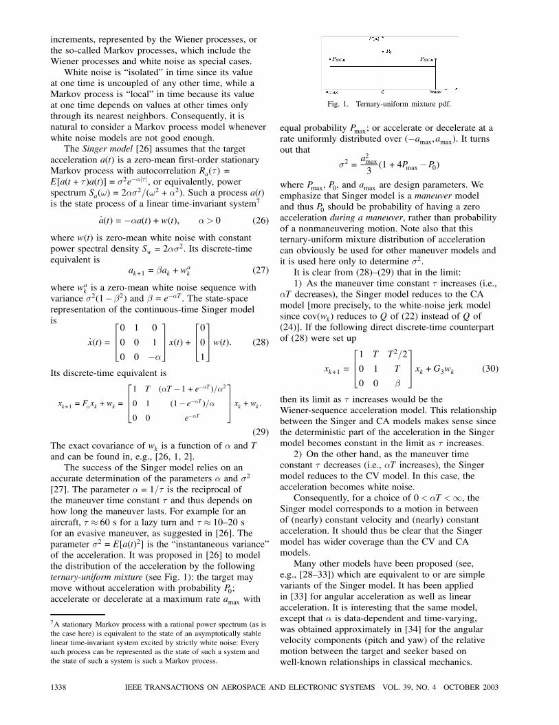
[27]. The parameter ®= 1=¿ is the reciprocal ofthe maneuver time constant ¿ and thus depends onhow long the maneuver lasts. For example for anaircraft, ¿ 60 s for a lazy turn and ¿ 10–20 sfor an evasive maneuver, as suggested in [26]. Theparameter ¾2 = E[a(t)2] is the “instantaneous variance”of the acceleration. It was proposed in [26] to modelthe distribution of the acceleration by the followingternary-uniform mixture (see Fig. 1): the target maymove without acceleration with probability P0;accelerate or decelerate at a maximum rate amax with

7A stationary Markov process with a rational power spectrum (as isthe case here) is equivalent to the state of an asymptotically stablelinear time-invariant system excited by strictly white noise: Everysuch process can be represented as the state of such a system andthe state of such a system is such a Markov process.

Fig. 1. Ternary-uniform mixture pdf.

equal probability Pmax; or accelerate or decelerate at arate uniformly distributed over ( amax,amax). It turnsout that

¾2 =a2max3(1+4Pmax P0)

where Pmax, P0, and amax are design parameters. Weemphasize that Singer model is a maneuver modeland thus P0 should be probability of having a zeroacceleration during a maneuver, rather than probabilityof a nonmaneuvering motion. Note also that thisternary-uniform mixture distribution of accelerationcan obviously be used for other maneuver models andit is used here only to determine ¾2.

It is clear from (28)–(29) that in the limit:1) As the maneuver time constant ¿ increases (i.e.,

®T decreases), the Singer model reduces to the CAmodel [more precisely, to the white-noise jerk modelsince cov(wk) reduces to Q of (22) instead of Q of(24)]. If the following direct discrete-time counterpartof (28) were set up

xk+1 =

1 T T2=2

0 1 T

0 0 ¯

xk +G3wk (30)

then its limit as ¿ increases would be theWiener-sequence acceleration model. This relationshipbetween the Singer and CA models makes sense sincethe deterministic part of the acceleration in the Singermodel becomes constant in the limit as ¿ increases.

2) On the other hand, as the maneuver timeconstant ¿ decreases (i.e., ®T increases), the Singermodel reduces to the CV model. In this case, theacceleration becomes white noise.

Consequently, for a choice of 0 < ®T < , theSinger model corresponds to a motion in betweenof (nearly) constant velocity and (nearly) constantacceleration. It should thus be clear that the Singermodel has wider coverage than the CV and CAmodels.

Many other models have been proposed (see,e.g., [28–33]) which are equivalent to or are simplevariants of the Singer model. It has been appliedin [33] for angular acceleration as well as linearacceleration. It is interesting that the same model,except that ® is data-dependent and time-varying,was obtained approximately in [34] for the angularvelocity components (pitch and yaw) of the relativemotion between the target and seeker based onwell-known relationships in classical mechanics.


The Singer acceleration model is a popular modelfor target maneuvers (see, e.g., [35–40], [1, 2]). Itwas the first model that characterizes the unknowntarget acceleration as a time-correlated (i.e., colored)stochastic process, and has served as a basis forfurther development of many effective maneuvermodels.The Singer model is in essence an a priori model

since it does not use online information about thetarget maneuver, although it can be made adaptivethrough an adaptation of its parameters ®, Pmax, P0,T, and/or amax. We cannot reasonably expect anya priori model to have a remarkable effectivenessfor the diverse acceleration situations of actualtarget maneuvers. As a consequence of its a priorinature, the Singer model is also symmetric in thatthe assumed ternary-uniform mixture distributionof the acceleration is symmetric. One of the mainshortcomings of the Singer model stems from thissymmetry; that is, the target acceleration has zeromean at any moment. Indeed, this is almost the bestone can do a priori without online information aboutthe target maneuver. Otherwise towards where shouldthe mean be? However, nothing really prevents usfrom using online information if we can withstand alittle more sophistication. Several more sophisticatedacceleration models have been proposed to remedythis shortcoming. They are described next.

E. Mean-Adaptive Acceleration Model

An acceleration model, called the “current” modelby its authors, proposed in [41], is in essence a Singermodel with an adaptive mean; that is, a Singer modelmodified to have a non-zero mean of the acceleration:a(t) = a(t) + a(t), where a(t) is the zero-mean Singeracceleration process, defined by (26), and a(t) is themean of the acceleration, artificially assumed constantover each sampling interval. Such a non-zero-meanacceleration satisfies

_a(t) = ®a(t)+w(t) or _a(t) = ®a(t)+®a(t)+w(t)

(31)

since _a(t) = _a(t) over any sampling interval. Theestimate ak of ak from all available online information(i.e., the sequence zk of observations through time k)is taken to be the “current” value of the mean ak+1,hence, the name. It is potentially more effective thanthe Singer model.The state-space representation of this model is

_x(t) =

0 1 0

0 0 1

0 0 ®

x(t) +

0

0

®

a(t) +

0

0

1

w(t)

(32)

excluding the time instants at which samples aretaken since a(t) is assumed piecewise constant. Thediscrete-time equivalent is

xk+1 = F®xk +

T2=2

T

1

(®T 1+ e ®T)=®2

(1 e ®T)=®

e ®T

ak +wk

(33)where F® was given in (29). These two equationsdiffer from the Singer model only in the additionalterms associated with a(t) and ak, respectively. Forexample, the noise w(t) and wk are identical tothose in the Singer model. Note also that this modelcorresponds to a Singer model with noise w of anon-zero adaptive mean.

A key underlying assumption of the “current”model in [41] (but not so stated explicitly) is thatak+1 = ak, or more specifically,

ak+1¢=E[ak+1 zk] = E[ak zk]

¢= ak (34)

where zk stands for all measurements through timetk. This is questionable and can actually be avoided.Since the last equation of (33) reads

ak+1 = e®Tak + (1 e ®T)ak +w

ak (35)

we propose to improve the “current” model byreplacing ak+1 = ak with the following recursion

ak+1 = E[ak+1 zk] = e ®TE[ak zk] + (1 e ®T)ak

= e ®Tak + (1 e ®T)ak: (36)

Such a relationship makes better sense because ak+1depends on the current estimate ak as well as pastinformation ak . However, what is resulting is nolonger a purely current model.

In the “current” model, the a priori (unconditional)probability density f(ak+1) of the accelerationak+1 at time k+1 in the Singer model is replacedby a conditional density f(ak+1 ak). Clearly, thisconditional density carries more accurate informationand is better to be used than the a priori density, asexplained before. The following conditional Rayleighdensity (see Fig. 2) was proposed in [41] for ak+1:

f(a ak) =

c 2k(amax a)exp

(amax a)2

2c2k

1(amax a) ak > 0

c 2k(a a max)exp

(a a max)2

2c2k

1(a a max) ak < 0

where 1( ) is the unit step function; a max is thenegative acceleration limit, not necessarily equal toamax; and ck is an ak-dependent parameter. Note

that the ternary-uniform distribution assumption inthe Singer model was made only out of the needto calculate the error variance of the acceleration.Similarly, this conditional Rayleigh assumption was


Fig. 2. Conditional Rayleigh model.

Fig. 3. Asymmetric pdfs of normal acceleration.

made for the sole purpose of obtaining the variance ofthe acceleration prediction, which turns out to be

¾2k¢=E[(ak+1 ak+1)

2 ak] =

4 ¼

¼(amax ak)

2 ak > 0

4 ¼

¼(a max + ak)

2 ak < 0:

This result is valid only under the simplifyingassumption that E[ak+1 zk] = E[ak+1 ak], which isthe case when ak is a sufficient statistic of z

k for ak+1.Applications of the “current” model can be found

in the literature, e.g., to a benchmark tracking problem[42].

F. Asymmetrically Distributed Normal AccelerationModel

Target acceleration can be decomposed alongtwo directions: lift (normal to the target velocity andwing directions for an aircraft) and thrust or drag(along the velocity direction). Each component canbe modeled by a time-correlated random process.The nonnormal component can be modeled well bythe Singer model. However, this is often not the casefor lift, which is usually the dominant one, especiallyduring a maneuver. Its direction is determined by thetarget aspect angle and its magnitude can be modeledas a colored random process with an asymmetricaldistribution. It was proposed in [43] that the normalacceleration an(t) be modeled as an asymmetric anddeterministic function of a zero-mean first-order

Gauss-Markov process b(t):

an(t) = ®+ ¯e°b(t) (37)

where ®,¯,° are design parameters, depending onthe particular target type; b(t) satisfies the equationof the Single model _b(t) = (1=¿)b(t) +w(t), where¿ is the correlation time constant of b(t), which ingeneral differs from that of an(t). As shown in Fig. 3,three typical choices of ®,¯,° and the corresponding(highly asymmetrical) probability density functions(pdfs) were given in [43], including one [(®,¯,°) =(8, 4,0:5)] that is considered typical of modernpiloted aircraft in evasive maneuvers.

Both pros and cons of this model stem from thefact that the parameters ®,¯,° are target-type specific.It is more accurate than the Singer model at thecost of designing these parameters, which requiresknowledge of the target type, obtained either a priorior a posteriori. The shortcoming of the Singer modelwith a symmetric pdf is overcome by the use ofadditional information of target type in this model.

Note that the temporal correlation of theacceleration in this model does not have a rationalpower spectrum and is much more complicatedthan in the Singer model. It would be interestingto compare this model with a Singer model of thenormal acceleration an having the initial asymmetricpdf an(t0) = ®+ ¯e

°b(t0) with the same parameters®,¯,° as above.


G. Markov Models for Oscillatory Targets

It is not uncommon in reality that accelerationalong one coordinate direction is oscillatory due to,e.g., wind sway or platform roll. The Singer model isnot very suitable for such practical maneuvers. Theautocorrelation of such acceleration may be describedby

Ra(¿) = ¾2ae

® ¿ cos(!c¿ )

= ¾2ae³!n ¿ cos(!n 1 ³2¿ )

!2n = ®2 +!2c ,³ = ®=!n

(38)

where ¾2a , ®, !c, ³, and !n are average power,damping coefficient, actual (damped) frequency,damping ratio, and undamped natural frequency ofthe target acceleration, respectively.Such an acceleration process is the response of a

second-order prewhitening system to zero-mean whitenoise input w(t) with power spectral density 2®¾2a . Ithas transfer function

H(s) =s+!n

s2 +2³!ns+!2n(39)

and is described by (see, e.g., [44, 12, 11])

_a(t)_d(t)

=0 1

!2n 2³!n

a(t)

d(t)+

1

(1 2³)!nw(t)

(40)where d(t) = _a(t) w(t), which can be calledacceleration drift. The state-space model for x=[x, _x, x,d] is

_x(t) = Ax(t)+Bw(t) =

0 1 0 00 0 1 00 0 0 10 0 !2n 2³!n

x(t)

+

001

(1 2³)!n

w(t): (41)

Note that the autocorrelation Ra(¿) is not periodicanymore if ³ 1. More generally, if the targetacceleration has autocorrelation

Ra(¿) =¾2acos µ

e ³!n ¿ cos(!n 1 ³2 ¿ µ) (42)

then the state-space model [44, 12, 11] is given by(41) with Bw(t) replaced by [0,0,b,c] w(t), where

b =2¾2acos µ

!n sin(' µ)

c =2¾2acos µ

!3n sin('+ µ)

'= tan 1 ³

1 ³2

(43)

and the corresponding transfer function of theprewhitening system is

H(s) =bs+ c

s2 +2³!ns+!2n: (44)

This model was utilized in a multiple-model tracker in[45].

The discrete-time equivalent of model (41) isfound to be

xk+1 =

1 T F13 F14

0

0 F(!c,®)

0

xk +wk (45)

where

F(!c,®) =

12®!c e ®T(2®!c cos !cT+ (®

2 !2c ) sin !cT)!c(®2 +!2c )

!c e ®T(!c cos !cT+®sin !cT)!c(®2 +!2c )

0e ®T(!c cos !cT+®sin !cT)

!c

e ®T sin !cT!c

0(®2 +!2c )e

®T sin !cT!c

e ®T(!c cos !cT ®sin !cT)!c

F13 =!c( 3®2 +!2c +2®

3T+2®!2c T) e ®T[!c( 3®2 +!2c )cos !cT ®(®2 3!2c )sin !cT]!c(®2 +!2c )2

F14 =!c( 2®+®2T+!2cT) + e

®T[2®!c cos !cT+(®2 !2c )sin !cT]

!c(®2 +!2c )2

(46)

and cov(wk) = SwT

0 eA¿BB (eA¿ ) d¿ can be found (e.g.,

by Mathematica) but is too tedious to be given here.A similar but slightly more sophisticated Markov

model was used in [11, 46] for a target trajectory withoscillations due to wind-induced bending. Assume thatthe bending is modeled by a second-order Markovsystem with undamped natural frequency !n anddamping ratio ³, along with a standard model ofwinds (i.e., a Singer model with correlation time


constant ¿ = 1=¹), such that the prewhitening systemhas the transfer function

H(s) =S1=2w s2

(s+¹)(s2 + 2³!ns+!2n)=

S1=2w s2

s3 +®s2 + ¯s+ °

(47)

where ®= ¹+2³!n, ¯ = !2n +2¹³!n, and ° = ¹!

2n .

This system is described by [11, 46]

_a

a...a

(t) =

0 1 0

0 0 1

° ¯ ®

a

_a

a

+

0

0

1

w(t)

(48)

where w(t) has power spectrum Sw = c3¾2 and ¾2 =

R(0) is the mean-square value of the target trajectorywith the following autocorrelation

R(¿) = c1e¹ ¿ + c2e

³!n ¿ cos(!n 1 ³2 ¿ µ)

(49)

which is a combination of a first-order term and asecond-order term. Here c1, c2, c3, and µ are constants,depending on ®, ¯, °, and ¾ [46]. Its discrete-timeequivalent can be found in [46].

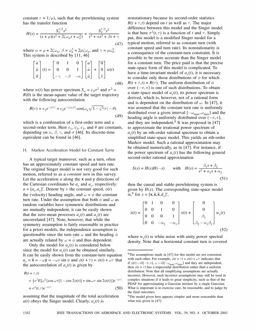
H. Markov Acceleration Model for Constant Turns

A typical target maneuver, such as a turn, oftenhas an approximately constant speed and turn rate.The original Singer model is not very good for suchmotion, referred to as a constant turn in this survey.Let the acceleration a along the x and y directions ofthe Cartesian coordinates be ax and ay, respectively:a= [ax,ay] . Denote by v the constant speed, Á(t)the (velocity) heading angle, and ! = _Á the constantturn rate. Under the assumption that both Á and ! asrandom variables have symmetric distributions andare mutually independent, it can be easily shownthat the zero-mean processes ax(t) and ay(t) areuncorrelated [47]. Note, however, that while thesymmetry assumption is fairly reasonable in practicefor a priori models, the independence assumption isquestionable since the turn rate ! and the heading Áare actually related by ! = _Á and thus dependent.Only the model for ax(t) is considered below

since the model for ay(t) can be obtained similarly.It can be easily shown from the constant-turn equationax = x= ! _y= !v sin Á and Á(t+ ¿) = Á(t) +!¿ thatthe autocorrelation of ax(t) is given by

R(t+ ¿ , t)

= 12v2E[!2 cos !¿[1 cos 2Á(t)]+ sin !¿ sin 2Á(t) ]e ® ¿

= ¾2(t,¿)e ® ¿ (50)

assuming that the magnitude of the total accelerationa(t) obeys the Singer model. Clearly, ax(t) is

nonstationary because its second-order statisticsR(t+ ¿ , t) depend on t as well as ¿ . The majordifference between this model and the Singer modelis that here ¾2(t,¿) is a function of t and ¿ . Simplyput, this model is a modified Singer model for atypical motion, referred to as constant turn (withconstant speed and turn rate). Its nonstationarity isa consequence of the constant-turn constraint. It ispossible to be more accurate than the Singer modelfor a constant turn. The price paid is that the precisestate-space form of this model is complicated. Tohave a time-invariant model of ax(t), it is necessaryto consider only those distributions of Á for whichR(t+ ¿ , t) = R(¿). The uniform distribution of Áover ( ¼,¼] is one of such distributions. To obtaina state-space model of ax(t), its power spectrum isderived, which is, however, not of a rational formand is dependent on the distribution of !. In [47], itwas assumed that the constant turn rate is uniformlydistributed over a given interval [ !max,!max] and theheading angle is uniformly distributed over ( ¼,¼],and they are independent.8 It was proposed in [47]to approximate the irrational power spectrum ofax(t) by an nth-order rational spectrum to obtain asimplified state-space model. This yields an nth-orderMarkov model. Such a rational approximation maybe obtained numerically, as in [47]. For instance, ifthe power spectrum of ax(t) has the following generalsecond-order rational approximation

S(s) =H(s)H( s) with H(s) =¯1s+¯2

s2 +®1s+®2

(51)

then the causal and stable prewhitening system isgiven by H(s). The corresponding state-space modelis,9 for x= [x, _x, x,dx] ,

_x(t) =

0 1 0 0

0 0 1 0

0 0 0 1

0 0 ®2 ®1

x(t) +

0

0

¯1

¯2 ®1¯1

wx(t)

(52)

where wx(t) is white noise with unity power spectraldensity. Note that a horizontal constant turn is covered

8The assumptions made in [47] for this model are not consistentwith each other. For example, Á(t+ ¿) = Á(t)+!¿ indicates thatif Á(t) [ ¼,¼], ! [ !max,!max] and they are independent,then Á(t+ ¿ ) has a trapezoidal distribution rather than a uniformdistribution. Note that all simplifying assumptions are actuallyincorrect. However, such incorrect assumptions may still be used incomplex situations if it leads to great simplicity, such as that of thePDAF for approximating a Gaussian mixture by a single Gaussian.What is important is to exercise care, be reasonable, and to judge bythe final outcomes.9The model given here appears simpler and more reasonable thanwhat was given in [47].


by the use of two uncoupled 4-dimensional modelshere, but actually it has a more accurate single5-dimensional model (see Section V).The second-order model given by (40) is a special

case of this general second-order model (52) with¯1 = 1, ¯2 = !n, ®1 = 2³!n, ®2 = !

2n . It follows from

(44) that if ¯1 = b, ¯2 = c, ®1 = 2³!n, ®2 = !2n the

target acceleration of this second-order Markovmodel has an oscillatory yet stationary autocorrelationgiven by (42), but the “exact” autocorrelation isgiven by (50), which is nonstationary. Note alsothat the above uniform distribution assumption ofthe turn rate is better replaced by those of [48],the Singer’s ternary-uniform mixture or its variants(e.g., a binary-uniform mixture or a single-point anduniform mixture) in many practical situations withadditional information of the turn rate.

I. Semi-Markov Jump Process Models

The Singer model approximates the targetacceleration as a continuous-time zero-mean Markovprocess. In practice, many target maneuvers involvean acceleration of a non-zero mean that may bereasonably assumed piecewise constant. However, thedifficulty here is that neither the time intervals overwhich the acceleration mean is piecewise constantnor the corresponding constant levels of the non-zeromean are known to a tracker.One of the simplest piecewise-constant random

processes, known as jump processes, is the so-calledsemi-Markov jump process (see [49] for anengineering-oriented description). It differs from aMarkov jump process only in that it has the Markovproperty10 if we consider only time instants of a jump,but not necessarily at other times, while a Markovjump process has the Markov property at all times.In other words, the past and the future states of asemi-Markov process may be coupled through thetime interval it stays in a state (called sojourn time)as well as the present state—its value at one time maydepend on values at other time instants through notonly its nearest neighbor state but also the sojourntime in the state.Several Markovian jump-mean acceleration

models have been proposed. The first was the onegiven in [50–53]. In this method, the unknowninput u(t) (assumed equal to the non-zero meanof the acceleration a) is modeled as a finite-statesemi-Markov jump process. Specifically, it wasassumed that the possible mean values of theacceleration are quantized into n known levelsa1, : : : , an, and the sequence u(tk) of the input

10That is, the past and future states are independent given thepresent state.

among these levels is a semi-Markov process (asojourn-time dependent Markov chain) with knowntransition probability P u(tk) = aj u(tk 1) = ai ,i,j = 1, : : : ,n, and sojourn-time probability distributionfunction Pij(¿) = P ¿ij ¿ , where ¿ij = tk tk 1 isthe sojourn time at level ai before it jumps to levelaj . Although the concept of such a semi-Markovjump process formalism was introduced in [50, 51],only exponentially distributed sojourn time wasconsidered therein. Note that if the sojourn time hasan exponential distribution, the input process u(t)is in fact Markov—the semi-Markov formulationis not needed.11 Moreover, the following modelof the acceleration a(t) as a combination of theabove jump-mean model and the Singer model wasproposed:

a(t) = ¯v(t) + u(t) + a(t) (53)

where a(t) is the Singer acceleration of (26), v isthe velocity, u(t) is the unknown acceleration mean,and ¯ is a drag coefficient. The correspondingcontinuous-time state-space representation is, forx= [x, _x, x] ,

_x(t) =

0 1 0

0 ¯ 1

0 0 ®

x(t) +

0

1

0

u(t)+

0

0

1

w(t):

(54)

In other words, the target acceleration is modeledas the Singer acceleration with non-zero meanthat is intended to be a semi-Markov (but actuallyMarkov) jump process. This model can be referredto as a Markovian jump-mean acceleration model.The unknown acceleration mean u(t) is estimatedby a weighted sum of the quantization levels:u(t) = n

i=1 aiP u(t) = ai z(s), s t , where asin a multiple-model formulation, the weight is theposterior probability of each level being the correctone, using all online measurements z(s),s t, as wellas the initial model probabilities, model transitionprobabilities, and the sojourn time distribution.Fig. 4 depicts some representative random processesas models of the target acceleration. Note that asemi-Markov jump process model for the accelerationis more effective than a white noise model with amean of random jumps.

Three important issues associated with this modelare the design of the input quantization levels, thetransition probabilities, and the sojourn time. This is

11A semi-Markov process with exponentially distributed sojourntime in each state is actually a Markov process. This is aconsequence of the unique memoryless property of the exponentialdistribution—knowledge of time already spent in a state doesnot alter distribution of a future state. Similarly, a discrete-timesemi-Markov process is Markov only if the sojourn time has ageometric distribution.


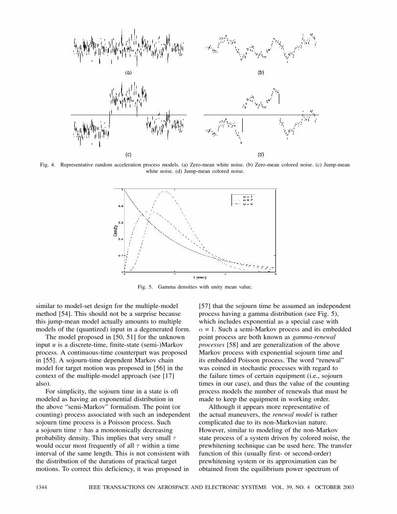
Fig. 4. Representative random acceleration process models. (a) Zero-mean white noise. (b) Zero-mean colored noise. (c) Jump-meanwhite noise. (d) Jump-mean colored noise.

Fig. 5. Gamma densities with unity mean value.

similar to model-set design for the multiple-modelmethod [54]. This should not be a surprise becausethis jump-mean model actually amounts to multiplemodels of the (quantized) input in a degenerated form.The model proposed in [50, 51] for the unknown

input u is a discrete-time, finite-state (semi-)Markovprocess. A continuous-time counterpart was proposedin [55]. A sojourn-time dependent Markov chainmodel for target motion was proposed in [56] in thecontext of the multiple-model approach (see [17]also).For simplicity, the sojourn time in a state is oft

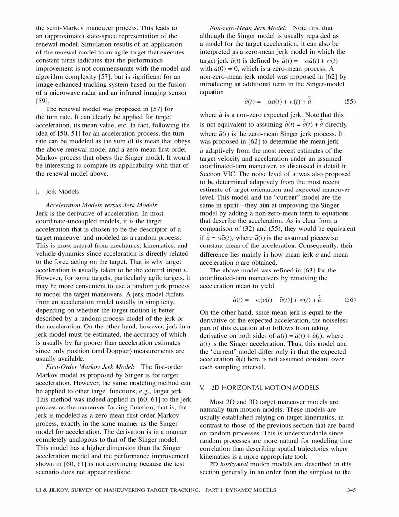
modeled as having an exponential distribution inthe above “semi-Markov” formalism. The point (orcounting) process associated with such an independentsojourn time process is a Poisson process. Sucha sojourn time ¿ has a monotonically decreasingprobability density. This implies that very small ¿would occur most frequently of all ¿ within a timeinterval of the same length. This is not consistent withthe distribution of the durations of practical targetmotions. To correct this deficiency, it was proposed in

[57] that the sojourn time be assumed an independentprocess having a gamma distribution (see Fig. 5),which includes exponential as a special case with®= 1. Such a semi-Markov process and its embeddedpoint process are both known as gamma-renewalprocesses [58] and are generalization of the aboveMarkov process with exponential sojourn time andits embedded Poisson process. The word “renewal”was coined in stochastic processes with regard tothe failure times of certain equipment (i.e., sojourntimes in our case), and thus the value of the countingprocess models the number of renewals that must bemade to keep the equipment in working order.

Although it appears more representative ofthe actual maneuvers, the renewal model is rathercomplicated due to its non-Markovian nature.However, similar to modeling of the non-Markovstate process of a system driven by colored noise, theprewhitening technique can be used here. The transferfunction of this (usually first- or second-order)prewhitening system or its approximation can beobtained from the equilibrium power spectrum of


the semi-Markov maneuver process. This leads toan (approximate) state-space representation of therenewal model. Simulation results of an applicationof the renewal model to an agile target that executesconstant turns indicates that the performanceimprovement is not commensurate with the model andalgorithm complexity [57], but is significant for animage-enhanced tracking system based on the fusionof a microwave radar and an infrared imaging sensor[59].The renewal model was proposed in [57] for

the turn rate. It can clearly be applied for targetacceleration, its mean value, etc. In fact, following theidea of [50, 51] for an acceleration process, the turnrate can be modeled as the sum of its mean that obeysthe above renewal model and a zero-mean first-orderMarkov process that obeys the Singer model. It wouldbe interesting to compare its applicability with that ofthe renewal model above.

J. Jerk Models

Acceleration Models versus Jerk Models:Jerk is the derivative of acceleration. In mostcoordinate-uncoupled models, it is the targetacceleration that is chosen to be the descriptor of atarget maneuver and modeled as a random process.This is most natural from mechanics, kinematics, andvehicle dynamics since acceleration is directly relatedto the force acting on the target. That is why targetacceleration is usually taken to be the control input u.However, for some targets, particularly agile targets, itmay be more convenient to use a random jerk processto model the target maneuvers. A jerk model differsfrom an acceleration model usually in simplicity,depending on whether the target motion is betterdescribed by a random process model of the jerk orthe acceleration. On the other hand, however, jerk in ajerk model must be estimated, the accuracy of whichis usually by far poorer than acceleration estimatessince only position (and Doppler) measurements areusually available.First-Order Markov Jerk Model: The first-order

Markov model as proposed by Singer is for targetacceleration. However, the same modeling method canbe applied to other target functions, e.g., target jerk.This method was indeed applied in [60, 61] to the jerkprocess as the maneuver forcing function; that is, thejerk is modeled as a zero-mean first-order Markovprocess, exactly in the same manner as the Singermodel for acceleration. The derivation is in a mannercompletely analogous to that of the Singer model.This model has a higher dimension than the Singeracceleration model and the performance improvementshown in [60, 61] is not convincing because the testscenario does not appear realistic.

Non-zero-Mean Jerk Model: Note first thatalthough the Singer model is usually regarded asa model for the target acceleration, it can also beinterpreted as a zero-mean jerk model in which thetarget jerk _a(t) is defined by _a(t) = ®a(t) +w(t)with a(0) = 0, which is a zero-mean process. Anon-zero-mean jerk model was proposed in [62] byintroducing an additional term in the Singer-modelequation

_a(t) = ®a(t)+w(t) + _a (55)

where _a is a non-zero expected jerk. Note that thisis not equivalent to assuming _a(t) = _a(t) + _a directly,where _a(t) is the zero-mean Singer jerk process. Itwas proposed in [62] to determine the mean jerk_a adaptively from the most recent estimates of thetarget velocity and acceleration under an assumedcoordinated-turn maneuver, as discussed in detail inSection VIC. The noise level of w was also proposedto be determined adaptively from the most recentestimate of target orientation and expected maneuverlevel. This model and the “current” model are thesame in spirit—they aim at improving the Singermodel by adding a non-zero-mean term to equationsthat describe the acceleration. As is clear from acomparison of (32) and (55), they would be equivalentif _a= ®a(t), where a(t) is the assumed piecewiseconstant mean of the acceleration. Consequently, theirdifference lies mainly in how mean jerk _a and meanacceleration a are obtained.

The above model was refined in [63] for thecoordinated-turn maneuvers by removing theacceleration mean to yield

_a(t) = ®[a(t) a(t)]+w(t) + _a: (56)

On the other hand, since mean jerk is equal to thederivative of the expected acceleration, the noiselesspart of this equation also follows from takingderivative on both sides of a(t) = a(t) + a(t), wherea(t) is the Singer acceleration. Thus, this model andthe “current” model differ only in that the expectedacceleration a(t) here is not assumed constant overeach sampling interval.

V. 2D HORIZONTAL MOTION MODELS

Most 2D and 3D target maneuver models arenaturally turn motion models. These models areusually established relying on target kinematics, incontrast to those of the previous section that are basedon random processes. This is understandable sincerandom processes are more natural for modeling timecorrelation than describing spatial trajectories wherekinematics is a more appropriate tool.

2D horizontal motion models are described in thissection generally in an order from the simplest to the


Fig. 6. Geometry of 2D target motion.

most sophisticated. 3D motion models, including thosefor (nonhorizontal) planar motion in the 3D space, aredescribed in the next section.Coordinate-coupled target models are highly

dependent on the choice of the state components.The choice of the state components (and implicitlythe respective kinematic model) is not a trivialproblem [64], where target dynamics, accuracy ofapproximations, sensor coordinate system, amongothers, must be taken into account.Various (noiseless part of) kinematic models

proposed for tracking of a target moving in thehorizontal plane can be comprised from the followingstandard curvilinear-motion model from kinematics(see Fig. 6):

_x(t) = v(t)cos Á(t) (57)

_y(t) = v(t)sin Á(t) (58)

_v(t) = at(t) (59)

_Á(t) = an(t)=v(t) (60)

where (x,y),v,Á are the target position in Cartesiancoordinates, ground speed (airspeed plus wind speed),and (velocity) heading angle, respectively, and at andan are the target tangential (along-track) and normal(cross-track) accelerations in the horizontal plane,respectively. This model is fairly general—it accountsfor along- and cross-track accelerations, and reducesto the following special cases:1) an = 0, at = 0—rectilinear, CV motion,2) an = 0, at = 0—rectilinear, accelerated motion

(CA motion if at = constant),3) an = 0, at = 0—circular, constant-speed motion

(CT motion if an = constant).The last case above with a constant an, which

has a constant speed and a constant turn rate, isreferred to as a constant turn (CT) in this surveybut is often referred to as a coordinated turn (CT)in target tracking, due to an abuse of terminology inour opinion. The motion referred to as a coordinatedturn in aviation is in fact not so simple and limited,which refers to certain constraints in terms of flightdynamics, rather than this purely kinematic model.(This is addressed in more detail in Section VIC,including a more reasonable definition in targettracking.) Such motion is preferably specified in termsof the turn rate ! = _Á.

The following variant of (60) was used in [65, 66]:_Á= an=v, where an = an sin( Ã) is the projection ofthe actual normal acceleration an on the horizontalplane and Ã is the roll (i.e., bank) angle. This variantmakes explicit the relationship between the normalacceleration in the horizontal plane and the actualnormal acceleration in a bank-to-turn horizontalmotion.

A. CT Models with Known Turn Rate

These models presume that the target moves with(nearly) constant speed v and (nearly) constant angular(turn) rate !. Assuming ! is known leads to (onlyfour-dimensional) state vector, e.g., x= [x, _x,y, _y] , inthe Cartesian coordinates. It follows immediately from(57)–(60) that such a circular motion is described by(5) with f(x,u, t) = [ _x, ! _y, _y,! _x] ; that is,

_x(t) =

_x(t)

! _y(t)

_y(t)

! _x(t)

+Bw(t) = A(!)x(t) +Bw(t)

(61)

A(!) =

0 1 0 0

0 0 0 !

0 0 0 1

0 ! 0 0

, B =

0 0

1 0

0 0

0 1

where white noise w = [wx,wy] has the powerspectral density diag[Sw,Sw]. This CT model is linearsince ! is known. Its discrete-time equivalent isfound to be

xk+1 = Fct(!)xk +wk

=

1sin !T!

01 cos !T

!

0 cos !T 0 sin !T

01 cos !T

!1

sin !T!

0 sin !T 0 cos !T

xk +wk

(62)where

Q = cov(wk) =

Sw

2(!T sin !T)!3

1 cos !T!2

0!T sin !T

!2

1 cos !T!2

T!T sin !T

!20

0!T sin !T

!22(!T sin !T)

!31 cos !T

!2

!T sin !T!2

01 cos !T

!2T

:

(63)


Its direct discrete-time counterpart (see [67, 1, 2]) isbetter known, given by (62), where wk is replaced bydiag[G2,G2]wk with G2 defined in (14) and a directlydefined cov(wk). The (zero-mean, Gaussian, white)noise w in the above is used to model the perturbationof the trajectory from the ideal CT motion.An approximation12 of the noiseless part of (62) is

[68, 69]:

Fct(!)xk

1 T 0 !T2=2

0 1 (!T)2=2 0 !T

0 !T2=2 1 T

0 !T 0 1 (!T)2=2

xk

(64)

=

x+[_x (1=2) _y!T]T_x _y!T (1=2) _x(!T)2

y+[_y+ (1=2) _x!T]T_y+ _x!T (1=2) _y(!T)2

which is a second-order polynomial in !. It providesa simple but less accurate alternative to the exact CTmodel. It is of certain value when a nonlinear tracker(e.g., extended Kalman filter (EKF)) is designed witha state vector that includes the (unknown) turn rate.However, it is valid only for !T 0, which may beviolated in many cases with large sampling interval T,such as in an air traffic control (ATC) system.In the rare cases where the constant turn rate is

(approximately) known a priori, the above CT modelgives good tracking performance. The necessity ofan exact knowledge about the value of the turn ratemakes the direct use of this model unrealistic for mostpractical applications. A natural idea is to replacethe above ! by its estimate, based on, e.g., the latestvelocity estimates, as used in [70, 67, 4]. However,this may inject unacceptably large errors into thesystem. Additional efforts are obviously requisite tomodel the motion with an unknown turn rate withinthis framework.Multiple Known Turn-Rate Models: Another

natural solution is based on the use of multiplemodels with different, fixed turn rates. This approachalleviates the effect of the uncertainty in the turn rateand takes advantage of the simple and linear form ofthe dynamic model (73) given the turn rate. In thisapproach, the sequence of turn rates !k is modeledas a Markov (or semi-Markov) chain taking valuesin the set !1,!2, : : : ,!n , governed by the transitionprobabilities P !k = !i !k 1 = !j , i,j = 1, : : : ,n, aswell as initial probabilities. This approach has beenwell established (see, e.g., [67, 4], and [68, 69]),mostly for ATC tracking applications. Therefore,a main application of this CT model with knownturn rate is serving as one or more (with different !values) models in a multiple-model architecture.

12By expanding sin µ and cos µ up to the second-order terms:sin µ µ and cos µ 1 µ2=2 for µ 0.

B. CT Models with Unknown Turn Rate

These models differ from the above CT modelsonly in that the turn rate is included as a statecomponent, to be estimated. As such, they aredescribed by (61) in continuous-time or (62) indiscrete-time plus an additional equation for !. Thetwo most popular models for ! are the Wiener processmodel

_!(t) = w!(t), in continuous time (65)

!k+1 = !k +w!,k, in discrete time (66)

and the first-order Markov process model

_!(t) =1¿!!(t)+w!(t), in continuous time

(67)

!k+1 = eT=¿!!k +w!,k, in discrete time (68)

where ¿! is the correlation time constant for the turnrate, and w is zero-mean white noise of a suitablelevel, which can be determined exactly the sameway as for the corresponding models for accelerationdescribed in the previous section. Some other modelsdescribed in the previous section can also be used forthe turn rate. For example, the renewal model of [57]is one of them.

Discretization of a continuous-time model herehas a unique issue: which discrete-time ! should beused in Fct(!) of (62)? The most popular way is to use!k here. Alternatively, it was proposed in [71] to use!k+1 in Fct(!) instead. This implicit method is morestable. The difference of the two schemes is somewhatsimilar in spirit to that of approximating a derivativeby the forward difference and backward differencein the finite difference method. With this roughanalogy in mind, it appears that replacing ! in (62)by ! = 1

2(!k +!k+1) would further improve accuracysince the center point is usually a better approximationthan either of the end points, more or less like thecentral difference is more accurate than the forwarddifference and backward difference at the cost of morecomputation (and possibly numerical instability). Forthe current problem, however, no extra computationis required by this new scheme if the procedure ofsolving the linearized equation as proposed in [71] isused, although possible numerical problems should bechecked. These three schemes lead to the followingthree different linearized models by the first-orderTaylor series expansions at [x,!] = [xk k, !k k] :

Fct(!k)xk = Fct(!k k)xk +F!(!k k)xk k(!k !k k)

Fct(!k+1)xk = Fct(!k k)xk +F!(!k k)

xk k(!k+1 !k k)

Fct(!)xk = Fct(!k k)xk +F!(!k k)xk k(! !k k)

(69)


where F!(!k k) = (@=@!)Fct(!) !=!k k . If (66) isused, however, these models have an identical stateprediction because

E[xk+1 zk] = E[Fct(!)xk zk] = Fct(!k k)xk k (70)

where zk stands for all measurements through timetk. This follows from E[! zk] = E[!k+1 zk] =E[!k zk] = !k k, a consequence of (66). Nevertheless,the corresponding covariances differ because differentmodels are used. That is why these models resultin very similar tracking performance, as reportedin [72] without explanation, for two IMM-EKF(interacting multiple model) algorithms using the firsttwo schemes above with real ATC data. The stateprediction would also be different if model (68) isused.We point out that it is theoretically more appealing

to obtain a discrete-time model for state vectorx= [x, _x,y, _y,!] by discretizing the followingcontinuous-time equations jointly:

[ _x, x, _y, y] (t) = ( _x, ! _y, _y,! _x) (t) +w(t) (71)

_!(t) = ®!(t) +w!(t) (72)

where ®= 0 or 1=¿!. It is reasonable to expect animprovement in performance with this alternative atthe price of an increased complexity.A continuous-time model is more accurate

than its discrete-time versions, but the latter areneeded for most applications. In the case wherethe continuous-time model is nonlinear, such asthe CT models with unknown turn rate, there arein general at least two approaches to acquiring itsdiscrete-time linear approximate models. Such modelsare needed in the application of a linear (e.g., Kalman)filter based nonlinear filtering technique. The firstis to linearize the nonlinear equation for the statefirst and then discretize the linearized differentialequation (by finding the solution via integration).This approach is more commonly used because itis easy. An alternative is to discretize the nonlinearstate-space equation first and then linearize thediscrete-time model. These two approaches arereferred to as discretized linearization and linearizeddiscretization, respectively, in [73, 64]. The secondapproach appears more accurate in general than thefirst since linearization usually lose more accuracythan discretization and thus should be done later.However, the second approach may not be tractablein general because discretization requires solvingthe nonlinear differential equation, which is often agreat challenge. Fortunately, for the CT motion withan unknown turn rate, the corresponding differentialequations for the state are simple and the solutioncan be readily obtained [73, 64]. The equations of thenearly CT model, obtained by the first approach, andsome performance comparison results are also givenin [73, 64].

As stated before, the choice of the state vector isnot trivial for the turn models. Essentially two classeshave been proposed. They differ in the representationof the velocity vector: in the Cartesian and polarcoordinates, respectively.

1) CT Models with Cartesian Velocity: Inthis model, the state vector is chosen to be x=[x, _x,y, _y,!] ; that is, the velocity vector ( _x, _y)is represented in the Cartesian coordinates.Consequently, a direct discrete-time version of themodel is given by (see [67, 2]):

xk+1 =Fct(! ) 0

0 ¯xk +diag[G2,G2,1]wk (73)

where ¯ = e ®T, ! = !k, !k+1, !, or somethingsimilar, G2 was given in (14), wk = [wx,wy,w!]k iszero-mean white noise with suitable statistics—theyare noise terms for acceleration in the x and ydirections and for turn rate.

This model is known to be used successfullyas one of models in numerous multiple-modelconfigurations (see, e.g., [74, 67, 2, 75, 4]).

2) CT Models with Polar Velocity: Obviously, thevelocity vector can also be represented in the polar

coordinates as [v,Á] in terms of speed v = _x2+ _y

2

and (velocity) heading angle Á= tan 1( _y= _x). The statevector is thus x= [x,y,v,Á,!] . The correspondingdifferential equation is given by (5) with f(x,u, t) =[v cos Á, v sin Á, 0, !, 0] ; that is

_x(t) = [v cos Á,v sin Á,0,!,0] +w(t) (74)

which follows immediately from (57)–(60) by setting! and v constant. By linearization first and thendiscretization, its discrete-time linearized model isgiven in [76] (see also [1]):

xk+1 =

x+(2=!)v sin(!T=2)cos(Á+!T=2)

y+(2=!)v, sin(!T=2)sin(Á+!T=2)

v

Á+!T

! k

+wk

(75)where wk is white noise with covariance

Q = diag0 0

0 0,T2¾2_v ,

T3¾2_!=3 T2¾2_!=2

T2¾2_!=2 T2¾2_!:

(76)

This model was successfully used as a building blockof a multiple-model algorithm for aircraft trackingapplication in an air defense system [77, 78].

The above model uses (65) for the turn rateper se. Instead, it may be better to use (67). Thecorresponding discrete-time model need be modifiedaccordingly.


The discretized linearization (i.e., discretizationafter linearization) alternative of this model can befound in [73, 64], along with a comparison of itsperformance with that of the linearized discretizationbased on a theoretical error analysis13 and MonteCarlo simulations. It was concluded therein thatwhenever possible linearized discretization ispreferable to discretized linearization. For the twoCT models with polar velocity, the former slightlyoutperforms the latter. It was also claimed therein thatthe CT model with polar velocity outperforms the CTmodel with Cartesian velocity.The use of the following variant of the above

CT model with polar velocity was reported in [79].Let the state vector be x= [x,y,v,Á,an] ; that is,replace the turn rate ! in the above model with thenormal (transversal) acceleration an. Then, it followsimmediately from (57)–(60) that the continuous-timestate-space model for the CT motion is given by(5) with f(x,u, t) = [v cos Á, v sin Á, 0, an=v, 0] . Adiscrete-time linear approximation of this model wasobtained based on a refined Euler-Cauchy scheme as[79]

xk+1 = xk +Tf(xk +12Tf(xk)) +wk (77)

followed by the standard EKF linearization, wherewk is white noise, obtained by a backward differenceof (the derivative of) the continuous-time whitenoise. Note that xk+1=2 xk +

12Tf(xk). A set of

such unknown acceleration models was includedin a tracker for ATC in [79] to account for possiblehorizontal motions.

C. Circular Motion Models

For a circular motion of a target, if its center wereknown, the simplest model would be to represent thecircle in the polar coordinates and place the origin atthe circle center. In this coordinate system, the targetdynamic model is linear for x= [½,µ, _µ]

xk+1 = diag[1,F2]xk +diag[1,G2=T]wk (78)

where F2 and G2 were given by (14) and wk is whitenoise. The corresponding measurement equationis pseudo-linear because the noise covariance isactually state dependent, described in detail in asubsequent part (see [15] for a preliminary version).As a result, the Kalman filter is not optimal butcan be nonetheless implemented straightforwardly.This maneuver-centered CT model was introducedin [80]. While the idea underlying this model isintuitively appealing, the inherent nonlinearity ofthe problem is not avoided. It obviously relies onan accurate determination of the center of the turn

13Based on estimation of the Frobenius norm of the neglected termsin the approximations.

in terms of the sensor coordinate system, which isinherently a nonlinear problem. The following simplegeometrically oriented procedure of estimating thecenter was proposed in [80]. Assume that each targetposition measurements are points on the circle; replacethe chord between any two consecutive measurementpoints with the straight line segment connecting them;the center can then be determined from the (average)intersection of the perpendicular bisectors of two ormore such straight line segments. An essentially thesame procedure was used in [81] for estimating thecenter. Note that using the center estimates injectsadditional nonlinearities into the system, which arenot accounted for in the above linear model.

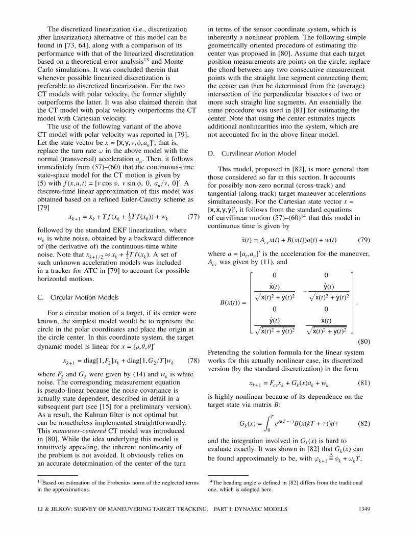
D. Curvilinear Motion Model

This model, proposed in [82], is more general thanthose considered so far in this section. It accountsfor possibly non-zero normal (cross-track) andtangential (along-track) target maneuver accelerationssimultaneously. For the Cartesian state vector x=[x, _x,y, _y] , it follows from the standard equationsof curvilinear motion (57)–(60)14 that this model incontinuous time is given by

_x(t) = Acvx(t) +B(x(t))a(t) +w(t) (79)

where a= [at,an] is the acceleration for the maneuver,Acv was given by (11), and

B(x(t)) =

0 0

_x(t)_x(t)2 + _y(t)2

_y(t)_x(t)2 + _y(t)2

0 0

_y(t)_x(t)2 + _y(t)2

_x(t)_x(t)2 + _y(t)2

:

(80)

Pretending the solution formula for the linear systemworks for this actually nonlinear case, its discretizedversion (by the standard discretization) in the form

xk+1 = Fcvxk +Gk(x)ak +wk (81)

is highly nonlinear because of its dependence on thetarget state via matrix B:

Gk(x) =T

0eA(T ¿)B(x(kT+ ¿))d¿ (82)

and the integration involved in Gk(x) is hard toevaluate exactly. It was shown in [82] that Gk(x) canbe found approximately to be, with 'k+1

¢=Ák +!kT,

14The heading angle Á defined in [82] differs from the traditionalone, which is adopted here.


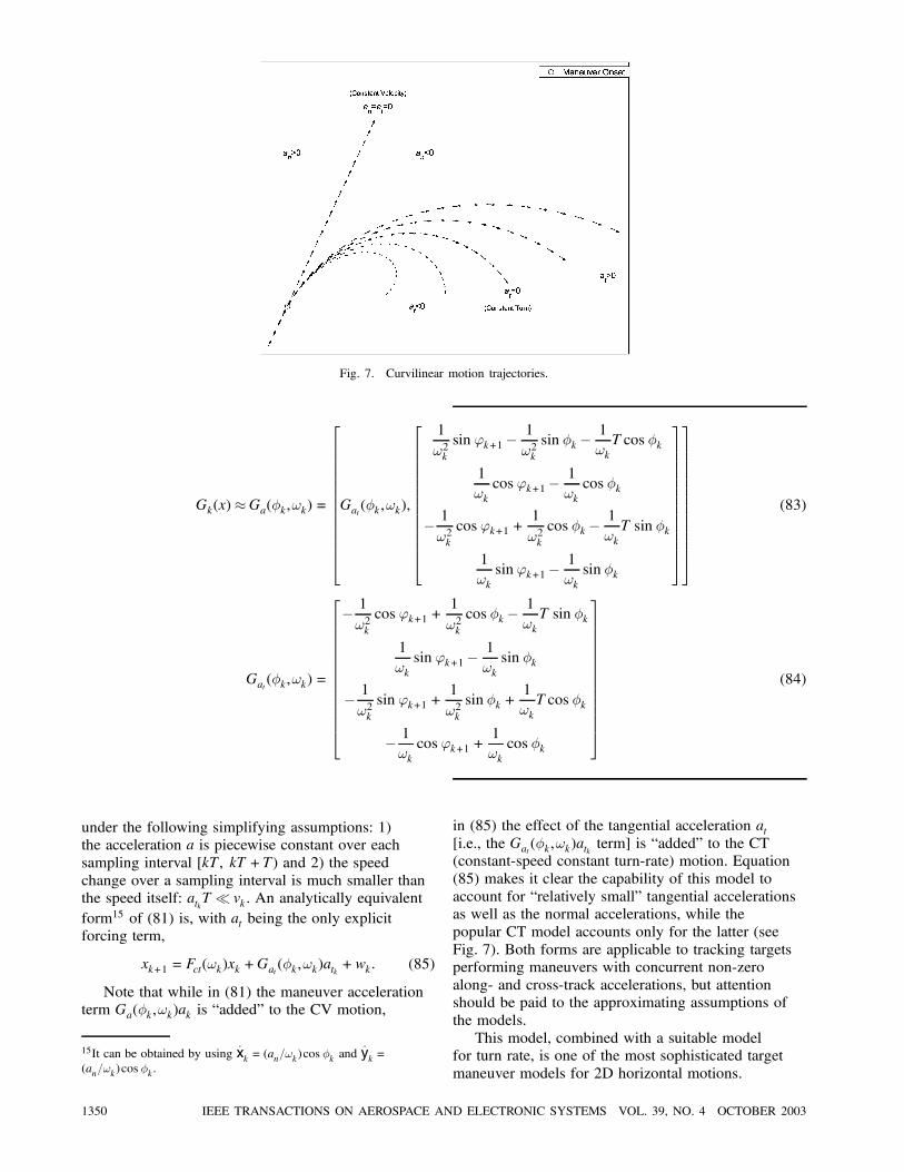
Fig. 7. Curvilinear motion trajectories.

Gk(x) Ga(Ák,!k) = Gat(Ák ,!k),

1!2ksin 'k+1

1!2ksin Ák

1!kTcos Ák

1!kcos 'k+1

1!kcos Ák

1!2kcos 'k+1 +

1!2kcos Ák

1!kT sin Ák

1!ksin 'k+1

1!ksin Ák

(83)

Gat(Ák,!k) =

1!2kcos 'k+1 +

1!2kcos Ák

1!kT sin Ák

1!ksin 'k+1

1!ksin Ák

1!2ksin 'k+1 +

1!2ksin Ák +

1!kTcos Ák

1!kcos 'k+1 +

1!kcos Ák

(84)

under the following simplifying assumptions: 1)the acceleration a is piecewise constant over eachsampling interval [kT, kT+T) and 2) the speedchange over a sampling interval is much smaller thanthe speed itself: atkT vk . An analytically equivalentform15 of (81) is, with at being the only explicitforcing term,

xk+1 = Fct(!k)xk +Gat(Ák,!k)atk +wk: (85)

Note that while in (81) the maneuver accelerationterm Ga(Ák,!k)ak is “added” to the CV motion,

15It can be obtained by using _xk = (an=!k)cos Ák and _yk =(an=!k)cos Ák:

in (85) the effect of the tangential acceleration at[i.e., the Gat(Ák,!k)atk term] is “added” to the CT(constant-speed constant turn-rate) motion. Equation(85) makes it clear the capability of this model toaccount for “relatively small” tangential accelerationsas well as the normal accelerations, while thepopular CT model accounts only for the latter (seeFig. 7). Both forms are applicable to tracking targetsperforming maneuvers with concurrent non-zeroalong- and cross-track accelerations, but attentionshould be paid to the approximating assumptions ofthe models.

This model, combined with a suitable modelfor turn rate, is one of the most sophisticated targetmaneuver models for 2D horizontal motions.


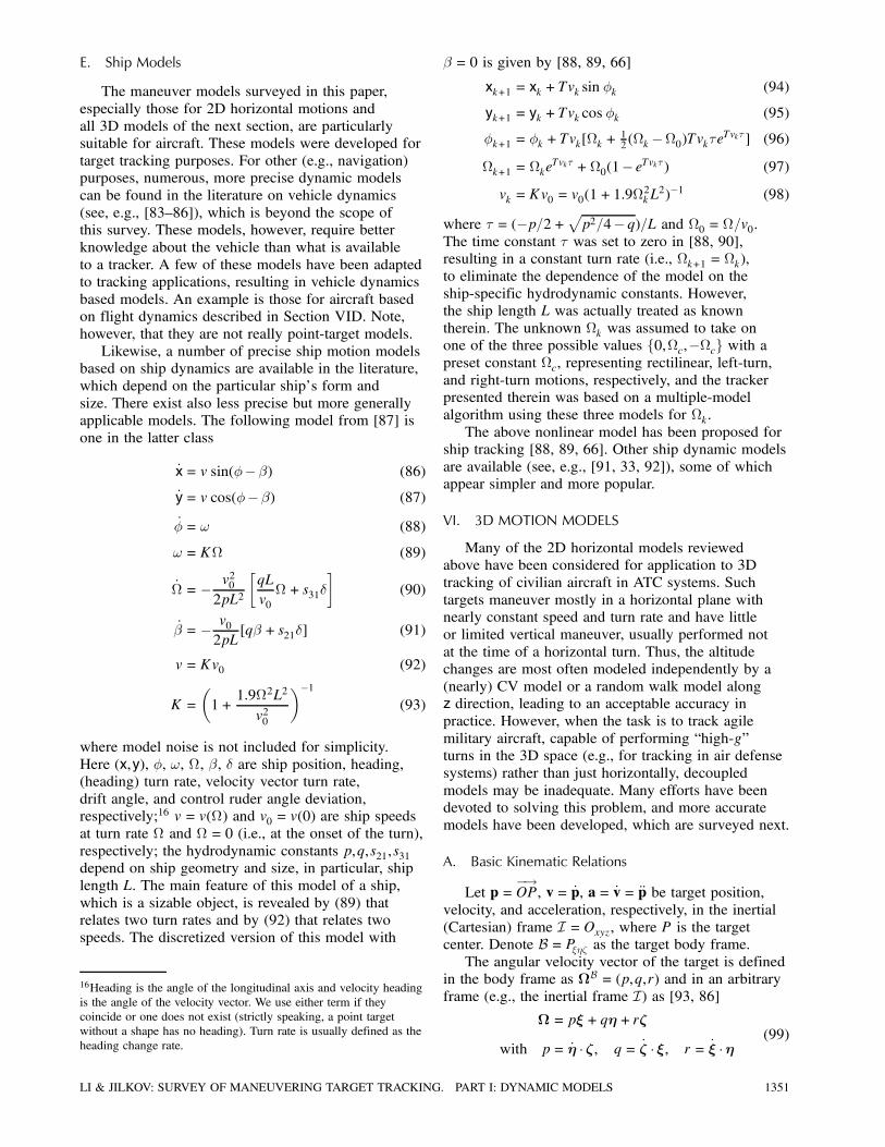
E. Ship Models

The maneuver models surveyed in this paper,especially those for 2D horizontal motions andall 3D models of the next section, are particularlysuitable for aircraft. These models were developed fortarget tracking purposes. For other (e.g., navigation)purposes, numerous, more precise dynamic modelscan be found in the literature on vehicle dynamics(see, e.g., [83–86]), which is beyond the scope ofthis survey. These models, however, require betterknowledge about the vehicle than what is availableto a tracker. A few of these models have been adaptedto tracking applications, resulting in vehicle dynamicsbased models. An example is those for aircraft basedon flight dynamics described in Section VID. Note,however, that they are not really point-target models.Likewise, a number of precise ship motion models

based on ship dynamics are available in the literature,which depend on the particular ship’s form andsize. There exist also less precise but more generallyapplicable models. The following model from [87] isone in the latter class

_x= v sin(Á ¯) (86)

_y= v cos(Á ¯) (87)

_Á= ! (88)

! = K (89)

_ =v202pL2

qL

v0+ s31± (90)

_ =v02pL

[q¯+ s21±] (91)

v = Kv0 (92)

K = 1+1:92L2

v20

1

(93)

where model noise is not included for simplicity.Here (x,y), Á, !, , ¯, ± are ship position, heading,(heading) turn rate, velocity vector turn rate,drift angle, and control ruder angle deviation,respectively;16 v = v() and v0 = v(0) are ship speedsat turn rate and = 0 (i.e., at the onset of the turn),respectively; the hydrodynamic constants p,q,s21,s31depend on ship geometry and size, in particular, shiplength L. The main feature of this model of a ship,which is a sizable object, is revealed by (89) thatrelates two turn rates and by (92) that relates twospeeds. The discretized version of this model with

16Heading is the angle of the longitudinal axis and velocity headingis the angle of the velocity vector. We use either term if theycoincide or one does not exist (strictly speaking, a point targetwithout a shape has no heading). Turn rate is usually defined as theheading change rate.

¯ = 0 is given by [88, 89, 66]

xk+1 = xk +Tvk sin Ák (94)

yk+1 = yk +Tvk cos Ák (95)

Ák+1 = Ák +Tvk[k +12(k 0)Tvk¿e

Tvk¿ ] (96)

k+1 = keTvk¿ +0(1 eTvk¿ ) (97)

vk = Kv0 = v0(1+1:92k L

2) 1 (98)

where ¿ = ( p=2+ p2=4 q)=L and 0 = =v0.The time constant ¿ was set to zero in [88, 90],resulting in a constant turn rate (i.e., k+1 = k),to eliminate the dependence of the model on theship-specific hydrodynamic constants. However,the ship length L was actually treated as knowntherein. The unknown k was assumed to take onone of the three possible values 0,c, c with apreset constant c, representing rectilinear, left-turn,and right-turn motions, respectively, and the trackerpresented therein was based on a multiple-modelalgorithm using these three models for k.

The above nonlinear model has been proposed forship tracking [88, 89, 66]. Other ship dynamic modelsare available (see, e.g., [91, 33, 92]), some of whichappear simpler and more popular.

VI. 3D MOTION MODELS

Many of the 2D horizontal models reviewedabove have been considered for application to 3Dtracking of civilian aircraft in ATC systems. Suchtargets maneuver mostly in a horizontal plane withnearly constant speed and turn rate and have littleor limited vertical maneuver, usually performed notat the time of a horizontal turn. Thus, the altitudechanges are most often modeled independently by a(nearly) CV model or a random walk model alongz direction, leading to an acceptable accuracy inpractice. However, when the task is to track agilemilitary aircraft, capable of performing “high-g”turns in the 3D space (e.g., for tracking in air defensesystems) rather than just horizontally, decoupledmodels may be inadequate. Many efforts have beendevoted to solving this problem, and more accuratemodels have been developed, which are surveyed next.

A. Basic Kinematic Relations

Let p=OP, v= _p, a= _v= p be target position,velocity, and acceleration, respectively, in the inertial(Cartesian) frame =Oxyz, where P is the targetcenter. Denote = P»´³ as the target body frame.

The angular velocity vector of the target is definedin the body frame as = (p,q,r) and in an arbitraryframe (e.g., the inertial frame ) as [93, 86]

= p»+ q´+ r³

with p= _ ³, q= _³ », r = _» ´(99)


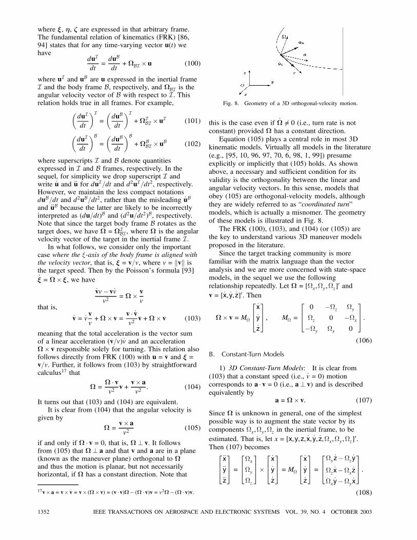
where », ´, ³ are expressed in that arbitrary frame.The fundamental relation of kinematics (FRK) [86,94] states that for any time-varying vector u(t) wehave

dudt

=dudt

+ u (100)

where u and u are u expressed in the inertial frameand the body frame , respectively, and is the

angular velocity vector of with respect to . Thisrelation holds true in all frames. For example,

dudt

=dudt

+ u (101)

dudt

=dudt

+ u (102)

where superscripts and denote quantitiesexpressed in and frames, respectively. In thesequel, for simplicity we drop superscript andwrite _u and u for du =dt and d2u =dt2, respectively.However, we maintain the less compact notationsdu =dt and d2u =dt2, rather than the misleading _uand u because the latter are likely to be incorrectlyinterpreted as (du=dt) and (d2u=dt2) , respectively.Note that since the target body frame rotates as thetarget does, we have = , where is the angularvelocity vector of the target in the inertial frame .In what follows, we consider only the important

case where the »-axis of the body frame is aligned withthe velocity vector, that is, » = v=v, where v = v isthe target speed. Then by the Poisson’s formula [93]_» = », we have

_vv v _vv2

=vv

that is,

_v= _vvv+ v=

v _vv2v+ v (103)

meaning that the total acceleration is the vector sumof a linear acceleration (v=v) _v and an acceleration v responsible solely for turning. This relation alsofollows directly from FRK (100) with u= v and » =v=v. Further, it follows from (103) by straightforwardcalculus17 that

= vv2

v+v av2

: (104)

It turns out that (103) and (104) are equivalent.It is clear from (104) that the angular velocity is

given by

=v av2

(105)

if and only if v= 0, that is, v. It followsfrom (105) that a and that v and a are in a plane(known as the maneuver plane) orthogonal to and thus the motion is planar, but not necessarilyhorizontal, if has a constant direction. Note that

17v a= v _v= v ( v) = (v v) ( v)v= v2 ( v)v.

Fig. 8. Geometry of a 3D orthogonal-velocity motion.

this is the case even if _ = 0 (i.e., turn rate is notconstant) provided has a constant direction.

Equation (105) plays a central role in most 3Dkinematic models. Virtually all models in the literature(e.g., [95, 10, 96, 97, 70, 6, 98, 1, 99]) presumeexplicitly or implicitly that (105) holds. As shownabove, a necessary and sufficient condition for itsvalidity is the orthogonality between the linear andangular velocity vectors. In this sense, models thatobey (105) are orthogonal-velocity models, althoughthey are widely referred to as “coordinated turn”models, which is actually a misnomer. The geometryof these models is illustrated in Fig. 8.

The FRK (100), (103), and (104) (or (105)) arethe key to understand various 3D maneuver modelsproposed in the literature.

Since the target tracking community is morefamiliar with the matrix language than the vectoranalysis and we are more concerned with state-spacemodels, in the sequel we use the followingrelationship repeatedly. Let = [x,y,z] andv= [_x, _y, _z] . Then

v=M

_x_y_z

, M =

0 z y

z 0 x

y x 0

:

(106)

B. Constant-Turn Models

1) 3D Constant-Turn Models: It is clear from(103) that a constant speed (i.e., _v = 0) motioncorresponds to a v= 0 (i.e., a v) and is describedequivalently by

a= v: (107)

Since is unknown in general, one of the simplestpossible way is to augment the state vector by itscomponents x,y,z in the inertial frame, to beestimated. That is, let x= [x,y,z, _x, _y, _z,x,y,z] .Then (107) becomes

x

y

z

=

x

y

z

_x_y_z

=M

_x_y_z

=

y _z z _y

z _x x _z

x _y y _x

:

(108)


If, in addition, is modeled as nearly constant(i.e., _ is white noise), then the continuous-time3D (nearly) CT model—which has (nearly) constantangular velocity and speed in the 3D space—is givenin the state space by

_x(t) =

0 I3 3 0

0 M 0

0 0 0

x(t)+

0

0

I3 3

w(t): (109)

This model is nonlinear since M of (106) depends onthe state components x,y,z.Note the difference between this model and

those based on (105): while v under (105), of (109), albeit nearly constant, is not necessarilyorthogonal to v, although v and a are orthogonal toeach other under (107). a is true for both models.To our knowledge, this simple 3D-CT model has notbeen considered in the tracking literature, despiteits generality: it can describe constant-speed motionalong non-zero torsion (nonplanar) curves.This model has a (nearly) constant speed and

angular velocity. An even more general model canbe developed by replacing _ = 0 with _! = 0, where! = , resulting in a general constant-turn (constantspeed and constant turn rate) model.2) Planar Constant-Turn Models: Under an

additional assumption v [or equivalently, (105)]as well as _ = 0, it follows from differentiation of(107) that

_a= a= ( v) = ( v) ( )v= !2v

(110)where the turn rate ! is given by

!¢= =

v av2

=v av2

=a

v: (111)

Therefore, the CT motion can be modeled by asecond-order Markov process

_a= !2v+w (112)

where w is white noise. As explained in footnote21 right after (123), this motion is (nearly) planarfor small w. This fact, along with _ = 0 and (105),implies that this is a planar constant speed andconstant turn rate (or angular velocity) motion. Hence,(112) is a (nearly) planar CT model.

This popular model can be traced back to [95, 100].A discussion of the vector models (107) and (110),along with an analysis and comparison with similarmodels, can be found in [99]. These models, alongwith several implementations, were reviewed in [1].

The state-space form of this model in the Cartesiancoordinates is clearly given by, with state x=[x,y,z, _x, _y, _z, x, y, z] ,

_x(t) =

0 I3 3 0

0 0 I3 3

0 !2I3 3 0

x(t) +

0

0

I3 3

w(t)

(113)or with state x= [x, _x, x,y, _y, y,z, _z, z] ,

_x(t) = diag[A(!),A(!),A(!)]x(t) +diag[B,B,B]w(t)

(114)

A(!) =

0 1 0

0 0 1

0 !2 0

, B =

0

0

1

(115)

where the white noise w(t) has power spectral densitymatrix diag[Sx,Sy,Sz]. Its discrete-time equivalentmodel [70] with state x= [x, _x, x,y, _y, y,z, _z, z]is18

xk+1 = diag[F(!),F(!),F(!)]xk +wk (116)

F(!) =

1sin !T!

1 cos !T!2

0 cos !Tsin !T!

0 ! sin !T cos !T

, cov(wk) = diag[SxQ(!),SyQ(!),SzQ(!)] (117)

Q(!) =

6!T 8sin !T+sin 2!T4!5

2 sin4(!T=2)!4

2!T+4 sin!T sin 2!T4!3

2 sin4(!T=2)!4

2!T sin 2!T4!3

sin2!T2!2

2!T+4 sin !T sin 2!T4!3

sin2!T2!2

2!T+sin 2!T4!

: (118)

18The covariance cov(wk) given here appears more reasonable thanwhat was suggested in [70, 1].


The motions in the x,y,z directions in this modelare coupled only through the common turn rate !.This model specifies a constant-turn motion in theso-called maneuver plane,19 defined by the velocityand acceleration vectors.This model relies on knowledge of !. If ! is

unknown, a straightforward way is to augment thestate vector by ! and estimate ! (see Section VB).This, however, increases the state dimension andmakes the model highly nonlinear. An alternative isto compute ! from the best speed and accelerationestimates by (111) so as to take advantage of thelinear structure of (116) at a given !. The use ofspeed and acceleration estimates will, however,inject additional errors into the model and resultin accuracy degradation, especially when theorthogonality property a v= 0 is severely violatedfor a constant-speed motion. A possible rescueis to impose a v= 0 as a kinematic constraint,which, however, turns the dynamic model into ahighly nonlinear one if it incorporates the constraintdirectly. Mainly to avoid this nonlinearity, analternative approach was adopted in [101, 70, 102,103] where the constraint was incorporated into apseudomeasurement model, described in detail in thesubsequent part of this survey on measurement models(its conference version is [15]).

C. Variable-Turn Models

The above models based on the constant-speedcondition (107) and the constant turn-rate assumptionare restrictive in describing the variety of possiblemaneuvers. More sophisticated and potentially moreaccurate models are surveyed next. They do notassume that a target moves with a constant turnand are thus capable of describing more complexmaneuvers.1) Planar Variable-Turn Model: By applying the

FRK to the target velocity vector v, we have

_v=dvdt

+ v: (119)

Differentiation and applying the FRK again yield

v=d2vdt2

+ _ v+2 _v ( v):

(120)

This equation describes a general motion of a rigidbody in space [96]. Under the orthogonal-velocity

19In the special case where the maneuver plane is horizontal, thismodel simplifies greatly and it is more commonly used than (themore general) model (57)–(60) for the derivation of some horizontalCT models [1]. In this case (i.e., at = 0 and ! = an=v), however,both models are essentially equivalent.

condition v, the angular velocity vector isgiven by (105). Substituting it in (120) results inmodeling the target acceleration as a second-orderMarkov process with state dependent coefficients20

in the inertial frame

_a= 2®a (2®2 +!2)v+w, w=d2vdt2

+ _ v

(122)where

!¢= =

v av2

, ®=v av2: (123)

This model, along with one in a slightly differentform in rotating line-of-sight (LOS) coordinates, wasproposed in [96]. Both forms were utilized therein fortwo highly accurate trackers.

The noise term w in (122) reflects the effect ofthe forces and moments applied to the target. It wasmodeled in [96] as zero-mean (Gaussian) white noisewith power spectral density matrix diag[Sx,Sy ,Sz]that is to be designed. The damping coefficient ® isa normalized target drag (i.e., the ratio of negativetangential acceleration to target speed). Both ® andturn rate ! can be interpreted as unknown modelparameters. As stated in [96], it can be shown that(122) defines zero-torsion (planar) trajectories (seeFig. 9) if and only if w= 0, that is, non-zero noisecomponents w account for out-of-plane motion.21 Assuch, (122) is a (nearly) planar variable-turn model ifits noise term w is small.

A possible enhancement of this model would be tomodel w in the body frame, which more accuratelyreflects the nature of the acting forces, and thentransform it to the inertial frame.

This planar variable-turn model is more generaland perhaps more accurate than the planar CT modelof (112). It reduces to the model (112) [with ! givenby (111)] for a CT motion under the constant-speedcondition (i.e., a v= 0). When the speed is notconstant, the damping term due to non-zero ® allowsthe model to automatically adapt itself to targetmaneuvers. Both ® and ! vanish for an unacceleratedmotion.

It is straightforward from (122) to obtain thefollowing continuous-time state-space form ofthis model in the inertial frame with state x=

20The formulation given here follows from [96, (5a) and (5b)] inview of the identity

a2

v2=

va

v2

2

(cos2 µ+sin2 µ) =v av2

2

+v av2

2

= ®2 +!2:

(121)21This implies that as a special case with ®= 0, (112) with w= 0describes a planar motion.


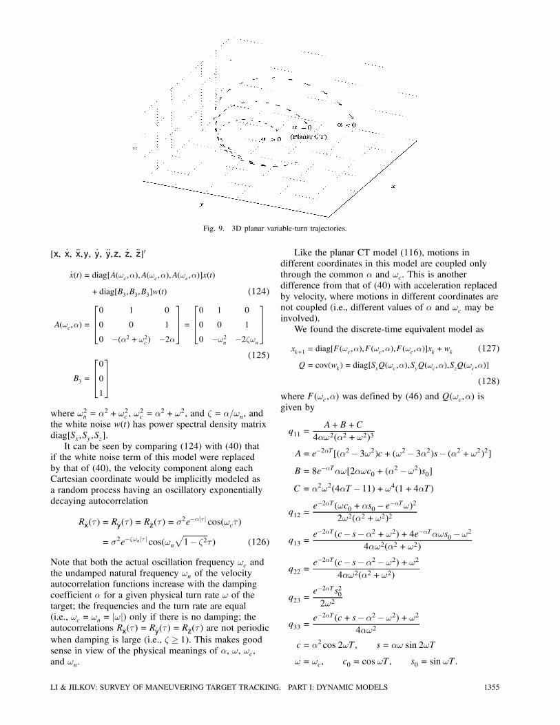
Fig. 9. 3D planar variable-turn trajectories.

[x, _x, x,y, _y, y,z, _z, z]

_x(t) = diag[A(!c,®),A(!c,®),A(!c,®)]x(t)

+diag[B3,B3,B3]w(t) (124)

A(!c,®) =

0 1 0

0 0 1

0 (®2 +!2c ) 2®

=

0 1 0

0 0 1

0 !2n 2³!n

(125)

B3 =

0

0

1

where !2n = ®2 +!2c , !

2c = ®

2 +!2, and ³ = ®=!n, andthe white noise w(t) has power spectral density matrixdiag[Sx,Sy,Sz].It can be seen by comparing (124) with (40) that

if the white noise term of this model were replacedby that of (40), the velocity component along eachCartesian coordinate would be implicitly modeled asa random process having an oscillatory exponentiallydecaying autocorrelation

R _x(¿) = R _y(¿) = R _z(¿) = ¾2e ® ¿ cos(!c¿)

= ¾2e ³!n ¿ cos(!n 1 ³2¿) (126)

Note that both the actual oscillation frequency !c andthe undamped natural frequency !n of the velocityautocorrelation functions increase with the dampingcoefficient ® for a given physical turn rate ! of thetarget; the frequencies and the turn rate are equal(i.e., !c = !n = ! ) only if there is no damping; theautocorrelations R _x(¿) = R _y(¿) = R _z(¿) are not periodicwhen damping is large (i.e., ³ 1). This makes goodsense in view of the physical meanings of ®, !, !c,and !n.

Like the planar CT model (116), motions indifferent coordinates in this model are coupled onlythrough the common ® and !c. This is anotherdifference from that of (40) with acceleration replacedby velocity, where motions in different coordinates arenot coupled (i.e., different values of ® and !c may beinvolved).

We found the discrete-time equivalent model as

xk+1 = diag[F(!c,®),F(!c,®),F(!c,®)]xk +wk (127)

Q = cov(wk) = diag[SxQ(!c,®),SyQ(!c,®),SzQ(!c,®)]

(128)

where F(!c,®) was defined by (46) and Q(!c,®) isgiven by

q11 =A+B+C

4®!2(®2 +!2)3

A= e 2®T[(®2 3!2)c+ (!2 3®2)s (®2 +!2)2]

B = 8e ®T®![2®!c0 + (®2 !2)s0]

C = ®2!2(4®T 11)+!4(1+4®T)

q12 =e 2®T(!c0 +®s0 e ®T!)2

2!2(®2 +!2)2

q13 =e 2®T(c s ®2 +!2) + 4e ®T®!s0 !2

4®!2(®2 +!2)

q22 =e 2®T(c s ®2 !2) +!2

4®!2(®2 +!2)

q23 =e 2®Ts202!2

q33 =e 2®T(c+ s ®2 !2) +!2

4®!2

c = ®2 cos 2!T, s= ®! sin 2!T

! = !c, c0 = cos !T, s0 = sin !T:


2) Coordinated-Turn Models: By the FRK (100)with u= ag

¢=a g, where g stands for the constant

gravitational acceleration in the inertial frame, wehave in the body frame

( _ag) =dagdt

+ ( ag) : (129)

Let T be the thrust (minus drag) and L the lift, along» and ´ directions, respectively. Then, we have ag =[T, L, 0] , = [p, q, r] , and

( ag) =M

T

L

0

, M =

0 r q

r 0 p

q p 0

:

(130)

Since ( _ag) = TBFIF _ag, where T

BFIF is the transform from

the inertial frame to the body frame, (129) becomes

TBFIF _ag =

_T_L

0

+

0 r q

r 0 p

q p 0

T

L

0

: (131)

An equivalent version of this general model in thebody frame for the so-called coordinated turn motionwas used in [62] to derive an equation for mean jerk.A class of motion in the 3D space, known as

coordinated turn, is defined (for aircraft) by thefollowing conditions, introduced originally in [62]and refined in [98]: 1) (mean) thrust T (minusdrag)—acceleration along the velocity direction—and(mean) lift L (acceleration normal to the aircraftwing plane) are constant; 2) (mean) roll angle Ã(angle around the longitudinal axis) is constant; and3) (mean) angle of attack and sideslip22 are zero.These conditions confine the (average) target motionto a plane, known as the maneuver plane. They areconsistent with the bank-to-turn characteristics offixed-wing aircraft. Clearly such an (average) motiondoes not necessarily have a constant turn rate orconstant speed.Under these coordinated turn conditions, we have

_T = 0, _L= 0, p= _ ³ = ( ´) ³ = 0 (because ,´, ³ are in the same plane orthogonal to »), and thus(131) becomes

_a= _ag = TIFBF

rL

rT

qT

, TIFBF = (TBFIF )

1 = (TBFIF ) :

(132)The expectation of this model is the meanjerk equation obtained in [62]. Its state-spacerepresentation can be obtained straightforwardly.

22The angle of attack is the angle between the heading and thevelocity vector projected onto the longitudinal symmetric planeand the sideslip is the angle between the velocity vector and thelongitudinal symmetric plane.

This coordinated turn model involves unknownparameters T, L, q, r, which can be obtained asfollows [62]. By the FRK (100) with u= v, we have_v= dv =dt+ v, which in the body frame is

dvdt

=

_v

0

0

+

0 r q

r 0 p

q p 0

v

0

0

(133)

where v is the target speed. On the other hand,(dv=dt) is the total acceleration a in the body frame,that is,

dvdt

= a =

T

L

0

+

g»

g´

g³

(134)

where g = [g»,g´,g³] is the gravitational accelerationin the body frame. It thus follows that

r = (L+ g´)=v, q= g³=v

T = _v g» , L= a g T:(135)

The target body frame is determined by the(estimated) velocity—to which the thrust T isparallel—and lift vector L.

Modeling the target accelerations in the bodyframe is simpler than in the inertial frame. However,the fact that it is in a frame different than the sensorinertial frame induces difficulties. In essence, allways around these difficulties involve explicitly orimplicitly conversion from one frame to the other,which can be done accurately in general only ifaccurate knowledge of the target position and modelparameters is available. In addition, while this modelis intuitive appealing, its implementation is rathercomplicated due to, e.g., its dependence on thrust, lift,and other parameters.

Furthermore, for the purpose of predicting targetposition in an antiaircraft fire control application(not as part of any filter), the following model inthe maneuver plane was employed in [62]. Theaircraft motion is described by a standard curvilinearmotion model of (57)–(60) in the maneuver plane withacceleration (at,an) determined by the thrust, lift, andgravity as

at = T+ gt, an = Lcos Ã+ gn (136)

where Lcos Ã is the projection of the lift along thenormal direction and Ã is the roll angle. Here, gt andgn are the gravity components along target velocityand normal directions, respectively, given by

gt = g» cos Á+ g´ sin Á, gn = g» sin Á+ g´ cos Á

(137)

where Á is the target velocity heading in the fixedCartesian frame in the maneuver plane. Likewise, thetarget position (x,y) (and speed v) in (57)–(60) are allin the fixed Cartesian frame in the maneuver plane.


Clearly, the approximate curvilinear modelof Section VD in the state-space form can beused here in the maneuver plane. However, thesmall speed-change assumption as well as thepiecewise-constant acceleration assumption on whichthis approximate model is based should be kept inmind. These assumptions are not valid for a largethrust and sampling interval.3) Generalized Coordinated-Turn Model:

Applying the FRK (100) to the target acceleration(with the gravity subtracted) ag = a g gives

_a=dagdt

+ (a g): (138)

Under the orthogonal-velocity condition v[i.e., (105)] and the constant acceleration conditiondag =dt = 0, (138) becomes

_a=v av2

(a g) (139)

which is the kinematic equation of [98]. It can beverified that the curvilinear trajectories generated by(139) have zero torsion, that is, they are confined tothe maneuver plane.If the gravity were not extracted, then the

orthogonal-velocity condition (105) and the constantacceleration condition da =dt = 0 (not equivalent todag =dt = 0) would lead to the following second-ordermodel in terms of the damping coefficient ® and turnrate !

_a=v av2

a=v av2a

a2

v2v= ®a (®2 +!2)v

(140)which is similar to (122).The conditions v and dag =dt = 0 are closely

related with coordinated turns. The constant thrustand lift condition validates assumption dag =dt= 0;the zero angle of attack and sideslip condition alignsthe »-axis of the real body frame (as defined in flightdynamics) with the assumed velocity-based bodyframe; and the constant roll angle condition validatesassumption v= 0 since the roll angular rate isthe projection of the angular velocity to the headingdirection: _Ã = (v=v). As such, a coordinated turnmotion can be readily described by (139) and thus(139) is a generalized model for coordinated turn andquasi coordinated turn motions.This model was originally proposed in [98],

implemented in [104], and later analyzed andvalidated in [99] by using real data of aircrafttrajectories.It was proposed in [104] to use a (vector-valued)

Singer process u to model the perturbations inacceleration in the body frame. As a result, thestate-space representation of this generalizedcoordinated turn model for the state vector x =

[p ,v ,a ,u ] is [104]

_x=

v

av av2

(a g) +T(v,a)u

°u

x+

0

0

0

I3 3

wb (141)

where p, v, a are the position, velocity, andacceleration vectors, respectively, in an inertial frameand T(v,a) = [t, b, n] is the coordinate transformationmatrix from the target body frame to the inertialframe, where t= v=v, b= (a g) v= (a g) v ,n= b t are the unit tangential, normal, and binormalvectors, respectively.

In this model, the (unperturbed) motions in thethree spatial directions are coupled and confined tothe maneuver plane, but not necessarily at a constantspeed. The time-correlated perturbation u accounts forthe (mostly out-of-plane) unmodeled motions and ismodeled in the body frame to be more precise. This,however, necessitates a coordinate transformation.This in turn introduces a dependency of the model onvelocity and acceleration estimates, which may leadto a model error and thus accuracy degradation. Thisgeneralized coordinated turn model does not estimatethe turn rate explicitly and is highly nonlinear.

While the constant-turn models of Section VIBand the coordinated-turn models of Section VIC aresimilar, they are based on two quite different ideas.The former are of kinematic type, which aim at fittingtypical target trajectories during a maneuver, whilethe development of the latter models relies on flightdynamics explicitly.

The generalized coordinated turn model (139) ismore convenient than the coordinated turn model(e.g., without the need to determine the thrust andlift). However, the planar VT model (122) is evenmore convenient for most applications. The underlyingassumptions for the constant-turn models of SectionVIB are that (105) holds and that the turn rate orthe angular velocity vector is constant. Note that itfollows from (107) and _ = 0 that _a= a. It differsfrom the generalized coordinated turn model only inthe lack of the g term, which is constant if isconstant. In particular, the two models coincide whenthe maneuver plane is horizontal.

Some other 3D target maneuver models are hardto be grouped into the above classes. For example, themaneuver model b = 0, e= 0 was proposed in [97]with a state x= [x,y,z,v,b, _b,e, _e] , where (x,y,z) and vare target position and speed, respectively, and b ande are the bearing and elevation of the velocity vector,respectively.

D. Flight Dynamics Based Models

An analysis of real trajectory data presented in[99] reveals that a target motion is not necessarily


confined to a plane in reality, but all the above modelsare exclusively or primarily for planar motionsand may be inadequate for more sophisticatedtarget motions. Models that incorporate sufficientout-of-plane motions may be more desirable in suchsituations. A class of more sophisticated models,based on flight dynamics, appears to be a betteralternative in this regard. The price is, however, adramatic increase in nonlinearity, state dimension,and number of design parameters largely uncertainin a noncooperative tracking environment. Also, theyare not really point-target models. We review thesemodels next.The basic idea of these models is to enhance

the modeling accuracy by not only exploring moredetailed flight-dynamics relationships but alsoexplicitly accounting for the aircraft’s controls. Werethe controls known to trackers, these models woulddescribe an aircraft motion more accurately than othermodels. So a fundamental issue here is the uncertaintyin the pilot’s control actions in a noncooperativeenvironment. Modeling these controls as randomprocesses is again a “standard” means to account forthis uncertainty. We consider the model of [105] toillustrate features of these models.The basis for this model is the rigid-body flight

dynamics model of aircraft motion [83], given in theform

_p= v (142)

_v= (c+ c®®+ c¯¯+C±±)v2 + cTT+ g (143)

_ = f() + (d®®+d¯¯+D+D±±)v2 +dTT

(144)

_©=G(©) (145)

with

f() =

(Ixx Iyy)qr=Ixx(Ixx Izz)rp=Ixx(Iyy Ixx)pq=Ixx

G(©) =

1 sin Á tanµ cos Á tanµ

0 cos Á sin Á

0 sin Á cos 1 µ cos Á cos 1 µ

(146)

where p= [x,y,z] is the position in the inertial frame, = [p,q,r] the angular velocity in the body frame,® the angle of attack, ¯ the sideslip, ± = [±A,±R ,±E]the angles of aileron, rudder, and elevator deflections,respectively, ©= [Ã,µ,Á] an attitude vector of theEuler angles: roll (bank angle) Ã, pitch µ, yaw(heading) Á, T the thrust, g the gravity, I the momentof inertia, and c, c®, c¯ , C±, cT, d®, d¯ , D±, dT arecoefficients. Equations (142)–(143) describe theaircraft body translational motion in the inertial frame,(144) is a moment equation describing the angularacceleration in the body frame, and (145) provides

the relationship between the Euler angles and theangular velocity. The aircraft body rotational motion((144)–(145)) strongly affects the translational motion((142)–(143)) through the dependence of the modelcoefficients c(©), c®(©), c¯(©), C±(©), cT(©) on theattitude angles © [105].

Given all the model coefficients, the uncertaintyof a maneuver boils down to that of the control input:thrust T and control angles ±. A state-space modelcan be developed in a trivial manner. For example,augment the state vector by T and ± and model theirvariations as zero-mean white noise processes [105].The resulting state vector x= [p ,v , ,© ,± ,T] is16-dimensional and the state-space model is givenby (142)–(145), with white noise added to (143) and(144), plus

_T = wT,_± =w± : (147)

The model (142)–(147) is quite general. Whatis crucial here is the determination of the modelcoefficients c(©), c®(©), c¯(©), C±(©), cT(©) and d®,d¯ ,D , D±,dT. This was done in [105] heuristicallybased on an analysis of a particular real trajectoryof a given aircraft. Caution has to be exercised in theapplication of such results to other situations.

A more rigorous model, albeit not general,was proposed in [106]. Under some simplifyingassumptions essentially the same as those for thecoordinated turn, an analytical expression of the lift asa function of the attitude angles © was derived, whichexplicitly describes the dependence of the acceleration_v on © in (143). The effects of the zero-mean thrust(minus drag) term T D and deflection angles werecollectively modeled as a first-order Markov (Singer)process °, governed by _° = (1=¿)°+w° , in place of(147) as above. The state vector x= [p ,v , ,© ,° ]is 15-dimensional.

In general, prediction accuracy of these modelsfor a target state can be dramatically improvedby accounting for the impact of the target attitudeangles on the target acceleration. In fact, thesemodels are clearly unobservable under position-onlymeasurements. Estimating the attitude angles ispossible if, in addition to the standard position (andpossibly velocity) measurements, direct attitudemeasurements are available. The use of attitudemeasurements was first suggested in [43] and furtherdeveloped in [107, 106, 108, 105], and others.

VII. CONCLUDING REMARKS

The target maneuver models developed for targettracking can be classified into 1D, 2D, and 3Dcategories, according to the coupling between motionsalong different coordinates.

The 1D models have no (or weak) coupling amongcoordinates. Most of them are based on modelingthe driving force (usually acceleration) of the target


maneuver as a random process without recourse to theactual target dynamics or kinematics directly. Thesemodels form three families, corresponding to threeclasses of random processes: white noise, Markovprocesses, and semi-Markov jump processes. Thesimplest white-noise family models the target positionderivative (or difference) of a certain order as whitenoise. It includes the classical CV and CA models.In the simple and widely used family of Markovprocesses, the target acceleration or jerk is modeledas a Markov process of various degrees of complexity.The most well-known representative of this familyis the Singer model. The semi-Markov jump processmodels are the most sophisticated family of the three.It has quite good potential, but the intricacy involvedin these models makes it hard for the practitioners toapply them.The 2D and 3D models differ from the 1D models

by not only their correlation across coordinates, butalso their explicit dependence on the target kinematicsand possibly dynamics. These models try to capturethe important characteristics of the target behaviorduring maneuvers, which typically involve variousturning motions. Many versions of (nearly) CT modelshave been developed. Few models are available thatare valid for other maneuver motions. Apart from thepopular CT models, it seems that the 2D approximatecurvilinear motion model and the planar variable-turnmodel of (122) deserve more attention than they havereceived due to their attractive simplicity, applicability,and flexibility.More accurate models are intuitively appealing, but

they also pose problems and challenges. For example,they are usually highly nonlinear and thus requireeffective nonlinear filtering algorithms; they may leadto poor tracking performance due to their dependenceon target state in the case of inaccurate state estimates,particularly for agile targets at a low data rate. Thatis partly why simple but less accurate models havetheir values and reasons to exist. While the choice ofa particular model depends certainly on the particularapplication, a good understanding of pros and cons ofeach model is nonetheless extremely helpful.Most of the models developed in the literature,

especially 2D and 3D models, are particularlysuitable for aircraft, although they are more or lessapplicable to many other targets. Many of theseaircraft models are fairly accurate, but they have acommon omission—wind effect is not consideredexplicitly. A reasonably large number of dynamicmodels have also been developed for ballistic targets(e.g., missiles), which will be covered separately ina subsequent part of this survey, of which [14] isa preliminary version. To our knowledge, however,few models have been developed that are particularlysuitable for other targets, such as submarines, ships,and ground targets. This deserves more effort.

ACKNOWLEDGMENTS

The authors would like to thank the followingpeople for their comments on the conference version[13] and/or draft of this paper: Yaakov Bar-Shalom,Edward Beadle, Jeff Bell, Bob Bishop, Henk Blom,Jean Dezert, Bob Fitzgerald, Keith Kastella, Gentervan Keuk, Ron Mahler, and Dave Sworder.

REFERENCES

[1] Blackman, S. S., and Popoli, R. F. (1999)Design and Analysis of Modern Tracking Systems.Boston, MA: Artech House, 1999.

[2] Bar-Shalom, Y., Li, X. R., and Kirubarajan, T. (2001)Estimation with Applications to Tracking and Navigation:Theory, Algorithms, and Software.New York: Wiley, 2001.

[3] Bar-Shalom, Y., and Li, X. R. (1993)Estimation and Tracking: Principles, Techniques, andSoftware.Boston, MA: Artech House, 1993. (Reprinted by YBSPublishing, 1998).

[4] Bar-Shalom, Y., and Li, X. R. (1995)Multitarget-Multisensor Tracking: Principles andTechniques.Storrs, CT: YBS Publishing, 1995.

[5] Bar-Shalom, Y. (Ed.) (1990)Multitarget-Multisensor Tracking: Advanced Applications.Norwood, MA: Artech House, 1990.

[6] Bar-Shalom, Y. (Ed.) (1992)Multitarget-Multisensor Tracking: Applications andAdvances, Vol. II, Norwwod, MA: Artech House, 1992.

[7] Bar-Shalom, Y., and Fortmann, T. E. (1988)Tracking and Data Association.New York: Academic Press, 1988.

[8] Blackman, S. S. (1986)Multiple Target Tracking with Radar Applications.Norwood, MA: Artech House, 1986.

[9] Farina, A., and Studer, F. A. (1985)Radar Data Processing, Vol. I: Introduction and Tracking,Vol. II: Advanced Topics and Applications.Letchworth, Hertfordshire, England: Research StudiesPress, 1985.

[10] Maybeck, P. S. (1982)Stochastic Models, Estimation and Control, Vols. II, III.New York: Academic Press, 1982.

[11] Maybeck, P. S. (1979)Stochastic Models, Estimation and Control, Vol. I.New York: Academic Press, 1979.

[12] Gelb, A. (1974)Applied Optimal Estimation.Cambridge, MA: MIT Press, 1974.

[13] Li, X. R., and Jilkov, V. P. (2000)A survey of maneuvering target tracking: Dynamicmodels.In Proceedings of the 2000 SPIE Conference on Signal andData Processing of Small Targets, Vol. 4048, Orlando, FL,Apr. 2000, 212–236.

[14] Li, X. R., and Jilkov, V. P. (2001)A survey of maneuvering target tracking—Part II:Ballistic target models.In Proceedings of the 2001 SPIE Conference on Signal andData Processing of Small Targets, Vol. 4473, San Diego,CA, July–Aug. 2001, 559–581.


[15] Li, X. R., and Jilkov, V. P. (2001)A survey of maneuvering target tracking—Part III:Measurement models.In Proceedings of the 2001 SPIE Conference on Signal andData Processing of Small Targets, Vol. 4473, San Diego,CA, July–Aug. 2001, 423–446.

[16] Li, X. R., and Jilkov, V. P. (2002)A Survey of maneuvering target tracking—Part IV:Decision-based methods.In Proceedings of the 2002 SPIE Conference on Signal andData Processing of Small Targets, Vol. 4728, Orlando, FL,Apr. 2002.

[17] Li, X. R., and Jilkov, V. P. (2003)A survey of maneuvering target tracking—Part V:Multiple-model methods.In Proceedings of the 2003 SPIE Conference on Signal andData Processing of Small Targets, Vol. 5204, San Diego,CA, Aug. 2003.

[18] Chan, Y. T., Hu, A. G. C., and Plant, J. B. (1979)A Kalman filter based tracking scheme with inputestimation.Transactions on Aerospace and Electronic Systems,AES-15, 2 (Mar. 1979), 237–244.

[19] Korn, J., Gully, S. W., and Willsky, A. S. (1982)Application of the generalized likelihood ratio algorithmto maneuver detection and estimation.In Proceedings of the 1982 American Control Conference,Arlington, VA, June 1982.

[20] Bogler, P. L. (1987)Tracking a maneuvering target using input estimation.Transactions on Aerospace and Electronic Systems,AES-23, 3 (May 1987), 298–310.

[21] Bogler, P. L. (1990)Radar Principles with Applications to Tracking Systems,New York: Wiley, 1990.

[22] Farooq, M., and Bruder, S. (1990)Information type filters for tracking a maneuvering target.Transactions on Aerospace and Electronic Systems, 26, 3(1990), 441–454.

[23] Whang, I. H., Lee, J., and Sung, T. (1994)Modified input estimation technique usingpseudoresiduals.Transactions on Aerospace and Electronic Systems, 30,1 (1994), 220–228; also published in 30, 2 (1994),591–598.

[24] Sung, T. K., and Lee, J. G. (1997)A decoupled adaptive tracking filter for real applications.Transactions on Aerospace and Electronic Systems, 33, 3(1997), 1025–1030.

[25] Lee, H., and Tahk, M-J. (1999)Generalized input-estimation technique for trackingmaneuvering targets.IEEE Transactions on Aerospace and Electronic Systems,35, 4 (1999), 1388–1402.

[26] Singer, R. A. (1970)Estimating optimal tracking filter performance formanned maneuvering targets.Transactions on Aerospace and Electronic Systems, AES-6(July 1970), 473–483.

[27] Singer, R. A., and Benhke, K. W. (1971)Real-time tracking filter evaluation and selection fortactical applications.Transactions on Aerospace and Electronic Systems, AES-7(Jan. 1971), 100–110.

[28] Pearson, J. B. (1970)Basic Studies in Airborne Radar Tracking Systems.Ph.D. dissertation, University of California at LosAngeles, 1970.

[29] Pearson, J. B., and Stear, E. B. (1974)Kalman filter applications in airborne radar tracking.Transactions on Aerospace and Electronic Systems, AES-10(1974), 319–329.

[30] Fitts, J. M. (1973)Aided tracking as applied to high accuracy pointingsystems.Transactions on Aerospace and Electronic Systems, AES-9(May 1973).

[31] Landau, M. (1976)Radar tracking of airborne targets.Presented at the National Aerospace and ElectronicsConference (NAECON), Dayton, OH, 1976.

[32] Blair, W. D., Watson, G. A., and Rice, T. R. (1991)Tracking maneuvering targets with an interactingmultiple model filter containing exponentially correlatedacceleration models.Southeastern Symposium on Systems Theory, Columbia,SC, Mar. 1991.

[33] Mandzuka, S. (2000)Ship tracking control: Optimal estimation of navigationparameters.In Proceedings of the 42th International SymposiumELMAR, Zadra, 2000.

[34] Ekstrand, B. (2001)Tracking filters and models for seeker applications.Transactions on Aerospace and Electronic Systems,AES-37, 3 (2001), 965–976.

[35] McAulay, R. J., and Denlinger, E. J. (1973)A decision-directed adaptive tracker.Transactions on Aerospace and Electronic Systems, AES-9,2 (Mar. 1973), 229–236.

[36] Cloutier, J. R., Evers, J. H., and Feeley, J. J. (1989)Assessment of air-to-air missile guidance and controltechnology.IEEE Control Systems Magazine, CSM-9 (Oct. 1989),27–34.

[37] Easthope, P. F., and Heys, N. W. (1994)Multiple-model target-oriented tracking system.In Proceedings of the 1994 SPIE Conference on Signal andData Processing of Small Targets, Vol. 2235, Apr. 1994.

[38] Costa, P. J. (1994)Adaptive model architecture and extended Kalman-Bucyfilters.Transactions on Aerospace and Electronic Systems, 30, 2(Apr. 1994), 525–533.

[39] D’Souza, C. N., McClure, M. A., and Cloutier, J. R. (1994)Spherical target state estimators.In Proceedings of 1994 American Control Conference,Baltimore, MD, June 1994, 1675–1679.

[40] Pulford, G., and La Scala, B. (1996)A survey of manoeuvring target tracking methods andtheir applicability to over-the-horizon radar.Technical Report CSSIP 14, Cooperative Research Centerfor Sensor Signal and Information Processing, Australia,July 1996.

[41] Zhou, H., and Kumar, K. S. P. (1984)A “current” statistical model and adaptive algorithm forestimating maneuvering targets.AIAA Journal of Guidance, 7, 5 (Sept.–Oct. 1984),596–602.

[42] Jilkov, V. P., Mihaylova, L. S., and Li, X. R. (1998)An alternative IMM solution to benchmark radar trackingproblem.In Proceedings of International Conference onMultisource-Multisensor Information Fusion, July 1998,924–929.


[43] Kendrick, J. D., Maybeck, P. S., and Reid, J. G. (1981)Estimation of aircraft target motion using orientationmeasurements.Transactions on Aerospace and Electronic Systems, AES-17(Mar. 1981), 254–260.

[44] Fitzgerald, R. J. (1967)Filtering horizon-sensor measurements for orbitalnavigation.Journal of Spacecraft and Rockets, 4, 4 (Apr. 1967),428–435.

[45] Wheaton, B. J., and Maybeck, P. S. (1995)Second-order acceleration model for an MMAE targettracker.Transactions on Aerospace and Electronic Systems, 31, 1(1995), 151–166.

[46] Ozkaya, B., and Arcasoy, C. (1998)Analytical solution of discrete colored noise ECAtracking filter.Transactions on Aerospace and Electronic Systems, 34, 1(1998), 93–102.

[47] Helferty, J. P. (1996)Improved tracking of maneuvering targets: The use ofturn-rate distriburions for acceleration modeling.Transactions on Aerospace and Electronic Systems, 32, 4(Oct. 1996), 1355–1361.

[48] Li, X. R., Zhao, Z-L., Zhang, P., and He, C. (2002)Model-set design for multiple-model estimation—Part II:Examples.In Proceedings of 2002 International Conferenceon Information Fusion, Annapolis, MD, July 2002,1347–1354.

[49] Howard, R. A. (1964)System analysis of semi-Markov processes.IEEE Transactions Military Electronics, MIL-8 (Apr.1964), 114–124.

[50] Moose, R. L., and Wang, P. L. (1973)An adaptive estimator with learning for a plant containingsemi-Markov switching parameters.IEEE Transactions on Systems, Man, Cybernetics, SMC-3(May 1973), 277–281.

[51] Moose, R. L. (1975)An adaptive state estimator solution to the maneuveringtarget problem.IEEE Transactions on Automatic Control, AC-20, 3 (June1975), 359–362.

[52] Gholson, N. H., and Moose, R. L. (1977)Maneuvering target tracking using adaptive stateestimation.Transactions on Aerospace and Electronic Systems, AES-13(May 1977), 310–317.

[53] Moose, R. L., VanLandingham, H. F., and McCabe, D. H.(1979)Modeling and estimation of tracking maneuvering targets.Transactions on Aerospace and Electronic Systems,AES-15, 3 (May 1979), 448–456.

[54] Li, X. R. (2002)Model-set design for multiple-model estimation—Part I.In Proceedings of 2002 International Conference onInformation Fusion, Annapolis, MD, July 2002, 26–33.

[55] Lim, S. S., and Farooq, M. (1991)Maneuvering target tracking using jump processes.In Proceedings of the 30th IEEE Conference on Decisionand Control, Brighton, UK, 1991, 2049–54.

[56] Campo, L., Mookerjee, P., and Bar-Shalom, Y. (1991)State estimation for systems with sojourn-time-dependentMarkov model switching.IEEE Transactions on Automatic Control, 36, 2 (Feb.1991), 238–243.

[57] Sworder, D. D., Kent, M., Vojak, R., and Hutchins, R. G.(1995)Renewal models for maneuvering targets.IEEE Transactions on Aerospace and Electronic Systems,31, 1 (Jan. 1995), 138–149.

[58] Cox, D. R. (1962)Renewal Theory.London: Methuen, 1962.

[59] Sworder, D. D., Singer, P. F., and Hutchins, R. G. (1993)Image-enhanced estimation methods.Proceedings of the IEEE, 81, 6 (June 1993), 797–812.

[60] Mehrotra, K., and Mahapatra, P. R. (1997)A jerk model to tracking highly maneuvering targets.Transactions on Aerospace and Electronic Systems, 33, 4(1997), 1094–1105.

[61] Mahapatra, P. R., and Mehrotra, K. (2000)Mixed coordinate tracking of generalized maneuveringtargets using acceleration and jerk models.Transactions on Aerospace and Electronic Systems, 36, 3(2000), 992–1001.

[62] Berg, R. F. (1983)Estimation and prediction for maneuvering targettrajectories.IEEE Transactions on Automatic Control, AC-28 (Mar.1983), 294–304.

[63] Song, T. L., Ahn, J., and Park, C. (1988)Suboptimal filter design with pseudomeasurements fortarget tracking.Transactions on Aerospace and Electronic Systems, 24 (Jan.1988), 28–39.

[64] Gustafsson, F., and Isaksson, A. J.Best choice of state variables for tracking coordinatedturns.In Proceedings of the 35th IEEE Conference on Decisionand Control, Kobe, Japan, Dec. 1996, 3145–3150.

[65] Semerdjiev, E., Mihaylova, L., and Li, X. R. (1999)An adaptive IMM estimator for aircraft tracking.In Proceedings of 1999 International Conference onInformation Fusion, Sunnyvale, CA, July 1999, 770–776.

[66] Semerdjiev, E., Mihaylova, L., and Li, X. R. (2003)An adaptive IMM estimation technique based onperturbation models.Submitted to Transactions on Aerospace and ElectronicSystems.

[67] Li, X. R., and Bar-Shalom, Y. (1993)Design of an interacting multiple model algorithm for airtraffic control tracking.IEEE Transactions on Control Systems Technology, 1, 3(Sept. 1993), 186–194; special issue on air traffic control.

[68] Dufour, F., and Mariton, M. (1991)Tracking a 3D maneuvering target with passive sensors.Transactions on Aerospace and Electronic Systems, 27, 4(July 1991), 725–739.

[69] Dufour, F., and Mariton, M. (1992)Passive sensor data fusion and maneuvering targettracking.In Y. Bar-Shalom (Ed.), Multitarget-Multisensor Tracking:Applications and Advances, Vol. II, Norwood, MA: ArtechHouse, 1992, ch. 3.

[70] Watson, G. A., and Blair, W. D. (1992)IMM algorithm for tracking targets that maneuverthrough coordinated turns.In Proceedings of the 1992 SPIE Conference on Signal andData Processing for Small Targets, Vol. 1698, 236–247.

[71] Kastella, K., and Biscuso, M. (1996)Tracking algorithms for air traffic control applications.Air Traffic Control Quarterly, 3, 1 (Jan. 1996), 19–43.


[72] Wang, H., Kirubarajan, T., and Bar-Shalom, Y. (1999)Precision large scale air traffic surveillance usingIMM/assignment estimators.Transactions on Aerospace and Electronic Systems, 35, 1(Jan. 1999), 255–266.

[73] Gustafsson, F. (2001)Adaptive Filtering and Change Detection.New York: Wiley, 2001.

[74] Vacher, P., Barret, I., and Gauvrit, M. (1992)Design of a tracking algorithm for an advanced ATCsystem.In Y. Bar-Shalom (Ed.), Multitarget-Multisensor Tracking:Applications and Advances, Vol. II, Norwood, MA: ArtechHouse, 1992, ch. 1.

[75] Lerro, D., and Bar-Shalom, Y. (1993)Interacting multiple model algorithm with targetamplitude feature.Transactions on Aerospace and Electronic Systems, 29, 2(Apr. 1993), 494–509.

[76] Gertz, J. L. (1989)Multisensor surveillance for improved aircraft tracking.Lincoln Laboratory Journal, 2, 3 (1989), 381–396.

[77] Busch, M., and Blackman, S. (1995)Evaluation of IMM filtering for an air defence systemapplication.In Proceedings of the 1995 SPIE Conference on Signal andData Processing of Small Targets, Vol. 2561, 435–447.

[78] Blackman, S. S., Busch, M. T., and Popoli, R. F. (1999)IMM/MHT solution to radar benchmark trackingproblem.Transactions on Aerospace and Electronic Systems, 35, 2(Apr. 1999), 730–737. Also appeared in Proceedings of1995 American Control Conference, Seattle, WA, June1995, 2606–2610.

[79] Blom, H. A. P., Hogendoorn, R. A., and van Doorn, B. A.(1992)Design of a multisensor tracking system for advanced airtraffic control.In Y. Bar-Shalom (Ed.), Multitarget-Multisensor Tracking:Applications and Advances, Vol. II, Norwood, MA: ArtechHouse, 1992, ch. 2.

[80] Roecker, J. A., and McGillem, C. D. (1989)Target tracking in maneuver centered coordinates.Transactions on Aerospace and Electronic Systems, 25(Nov. 1989), 836–843.

[81] Kawase, T., Tsurunosono, H., Ehara, N., and Sasase, I.(1998)Two-stage Kalman estimator using an advanced circularprediction for tracking highly maneuvering targets.In Proceedings of ICASSP98, 1998.

[82] Best, R. A. and Norton, J. P. (1997)A new model and efficient tracker for a target withcurvilinear motion.Transactions on Aerospace and Electronic Systems, 33, 3(July 1997), 1030–1037.

[83] Roskam, J. (1979)Airplane Flight Dynamics and Automatic Control, Part I.Roskam Aviation and Engineering Corp., Lawrence, KS,1979.

[84] Regan, F. J., and Anandakrishnan, S. M. (1993)Dynamics of Atmospheric Re-Entry.New York: AIAA, New York, 1993.

[85] Etkin, B., and Reid, L. D. (1996)Dynamcis of Flight: Stability and Control.New York: Wiley, 1996.

[86] Boiffier, J-L. (1998)The Dynamics of Flight: The Equations.New York: Wiley, 1998.

[87] Pershitz, R. (1973)Ship’s maneuverability and control.Leningrad, USSR: Sudostroenie, 1973.

[88] Semerdjiev, E., Mihaylova, L., and Semerdjiev, T. (1998)Manoeuvring ship model identification and interactingmultiple model tracking algorithm design.In Proceedings of 1998 International Conference onInformation Fusion, Las Vegas, NV, July 1998, 968–973.

[89] Semerdjiev, E., and Mihaylova, L. (2000)Variable- and fixed-structure augmented interactingmultiple model algorithm for manoeuvring ship trackingbased on new ship models.International Journal of Applied Mathematics andComputers, 10 (2000), 591–604.

[90] Semerdjiev, E., and Mihaylova, L. (1998)Adaptive interacting multiple model algorithm formanoeuvring ship tracking.In Proceedings of 1998 International Conference onInformation Fusion, Las Vegas, NV, July 1998, 974–979.

[91] Tzeng, C-Y., and Chen, J-F. (1999)Fundamental properties of linear ship steering dynamicmodels.Journal of Marine Science and Technology, 7, 2 (1999),79–88.

[92] Skjetne, R., and Fossen, T. I. (2001)Nonlinear maneuvering and control of ships.In Proceedings of Oceans 2001 MTS/IEEE Conference,Vol. 3, Nov. 2001, 1808–1815.

[93] Miele, A. (1962)Flight Mechanics: Theory of Flight Paths, Vol. 1.Reading, MA: Addison-Wesley, 1962.

[94] Hauser, W. (1965)Introduction to the Principles of Mechanics.New York: Wiley, 1965.

[95] Bryan, R. S. (1980)Cooperative estimation of targets by multple aircraft.M.S. thesis, Air Force Institute of Technology,Wright-Patterson AFB, Ohio, June, 1980.

[96] Asseo, S. J., and Ardila, R. J. (1982)Sensor independant target state estimator design andevaluation.In Procceedings of the National Aerospace and ElectronicsConference (NAECON), 1982, 916–924.

[97] Bullock, T. E., and Sangsuk-Iam, S. (1984)Maneuver detection and tracking with a nonlinear targetmodel.In Proceedings of the 23rd IEEE Conference on Decisionand Control, Las Vegas, NV, Dec. 1984.

[98] Bishop, R. H., and Antoulas, A. C. (1994)Nonlinear approach to the aircraft tracking problem.AIAA Journal of Guidance, Control and Dynamics, 17,5 (1994), 1124–1130. Also in Proceedings of the 1991AIAA Guidance, Navigation and Control Conference, NewOrleans, LA, Aug. 1991, 692–703.

[99] Nabaa, N., and Bishop, R. H. (2000)Validation and comparison of coordinated turn aircraftmaneuver models.Transactions on Aerospace and Electronic Systems, 36, 1(Jan. 2000), 250–259.

[100] Maybeck, P. S., Worsley, W. H., and Flynn, P. M. (1982)Investigation of constant turn-rate dynamics for airbornevehicle tracking.In Proceedings of the National Aerospace and ElectronicsConference (NAECON), 1982, 896–903.

[101] Tahk, M., and Speyer, J. L. (1990)Target tracking subject to kinematic constrants.IEEE Transactions on Automatic Control, 35 (Mar. 1990),324–326.


[102] Alouani, A. T., and Blair, W. D. (1991)Use of a kinematic constraint in tracking constant speed,maneuvering targets.In Proceedings of 30th IEEE Conference on Decision andControl, Brighton, England, Dec. 1991, 1055–1058.

[103] Alouani, A. T., and Blair, W. D. (1993)Use of a kinematic constraint in tracking constant speed,maneuvering targets.IEEE Transactions on Automatic Control, 38, 7 (July1993), 1107–1111.

[104] Nabaa, N., and Bishop, R. (1999)Solution to a multisensor tracking problem with sensorregistration errors.Transactions on Aerospace and Electronic Systems, 35, 1(1999), 354–362.

[105] Mook, D. J., and Shyu, I-M. (1992)Nonlinear aircraft tracking filter utilizing control variableestimation.AIAA Journal of Guidance, 15, 1 (Jan.–Feb. 1992),228–237.

[106] Andrisani, D., Kuhl, F. P., and Gleason, D. (1986)A nonlinear tracker using attitude measurements.Transactions on Aerospace and Electronic Systems, 22(Sept. 1986), 533–539.

[107] Lefas, C. C. (1984)Using roll-angle measurement to track aircraft maneuvers.Transactions on Aerospace and Electronic Systems, AES-20(Nov. 1984), 672–681.

[108] Andrisani, D., Kim, E. T., Schierman, J., and Kuhl, F. P.(1991)A nonlinear helicopter tracker using attitudemeasurements.Transactions on Aerospace and Electronic Systems, 27 (Jan.1991), 40–47.


X. Rong Li (S’90—M’92—SM’95) received the B.S. and M.S. degrees fromZhejiang University, Hangzhou, Zhejiang, PRC, in 1982 and 1984, respectively,and the M.S. and Ph.D. degrees from the University of Connecticut, Storrs, in1990 and 1992, respectively.He joined the Department of Electrical Engineering, University of New

Orleans in 1994, where he is now university research professor, department chair,and director of information and systems laboratory. During 1986–1987 he didresearch on electric power at the University of Calgary, AB, Canada. He was anassistant professor at the University of Hartford, West Hartford, CT, from 1992to 1994. His current research interests include signal and data processing, targettracking and information fusion, stochastic systems, statistical inference, andelectric power.Dr. Li has authored or coauthored four books: Estimation and

Tracking (with Yaakov Bar-Shalom, Norwood, MA: Artech House, 1993),Multitarget-Multisensor Tracking (with Yaakov Bar-Shalom, YBS Publishing,1995), Probability, Random Signals, and Statistics (CRC Press, 1999), andEstimation with Applications to Tracking and Navigation (with Yaakov Bar-Shalomand T. Kirubarajan, Wiley, 2001); six book chapters; and more than 160 journaland conference proceedings papers.Dr. Li has served the International Society of Information Fusion as the

president (2003), vice president (1998–2002) and a member of board of directors(since 1998); served as general chair for 2002 International Conference onInformation Fusion, and steering chair or general vice-chair for 1998, 1999, and2000 International Conferences on Information Fusion; served IEEE Transactionson Aerospace and Electronic Systems as an associate editor from 1995 to 1996and as editor since 1996; served Communications in Information and Systemsas an editor since 2001; received a CAREER award and an RIA award fromthe U.S. National Science Foundation. He received 1996 Early Career Awardfor Excellence in Research from the University of New Orleans and has givennumerous seminars and short courses in U.S., Europe and Asia. He won severaloutstanding paper awards, is listed in Marquis’ Who’s Who in America and Who’sWho in Science and Engineering, and consulted for several companies.

Vesselin P. Jilkov (M’01) received his B.S. and M.S. degree in mathematicsfrom the University of Sofia, Bulgaria in 1982, the Ph. D. degree in the technicalsciences in 1988, and the academic rank senior research fellow of the BulgarianAcademy of Sciences in 1997.He was a research scientist with the R&D Institute of Special Electronics,

Sofia, (1982–1988) where he was engaged in research and development of radartracking systems. From 1989 to 1999 he was a research scientist with the CentralLaboratory for Parallel Processing—Bulgarian Academy of Sciences, Sofia,where he worked as a key researcher in numerous academic and industry projects(Bulgarian and international) in the areas of Kalman filtering, target tracking,multisensor data fusion, and parallel processing. Since 1999 Dr. Jilkov has beenwith the Department of Electrical Engineering, University of New Orleans, wherehe is currently an assistant professor, and is engaged in teaching and conductingresearch in the areas of hybrid estimation and target tracking. His current researchinterests include stochastic systems, nonlinear filtering, applied estimation, targettracking, information fusion.Dr. Jilkov is author/coauthor of over 50 journal articles and conference papers.

He is a member of ISIF (International Society of Information Fusion).


Survey of Maneuvering Target Tracking. Part I: … · applicability of a target dynamic model for a...

Documents

Transcript of Survey of Maneuvering Target Tracking. Part I: … · applicability of a target dynamic model for a...