Survey Methodology 45-1
191
Survey Methodology Catalogue no. 12-001-X ISSN 1492-0921 Survey Methodology 45-1 Release date: May 7, 2019
Transcript of Survey Methodology 45-1

Survey Methodology
Catalogue no. 12-001-X ISSN 1492-0921
Survey Methodology45-1
Release date: May 7, 2019

Published by authority of the Minister responsible for Statistics Canada
© Her Majesty the Queen in Right of Canada as represented by the Minister of Industry, 2019
All rights reserved. Use of this publication is governed by the Statistics Canada Open Licence Agreement.
An HTML version is also available.
Cette publication est aussi disponible en français.
How to obtain more informationFor information about this product or the wide range of services and data available from Statistics Canada, visit our website, www.statcan.gc.ca. You can also contact us by Email at [email protected] Telephone, from Monday to Friday, 8:30 a.m. to 4:30 p.m., at the following numbers:
• Statistical Information Service 1-800-263-1136 • National telecommunications device for the hearing impaired 1-800-363-7629 • Fax line 1-514-283-9350
Depository Services Program
• Inquiries line 1-800-635-7943 • Fax line 1-800-565-7757
Standards of service to the publicStatistics Canada is committed to serving its clients in a prompt, reliable and courteous manner. To this end, Statistics Canada has developed standards of service that its employees observe. To obtain a copy of these service standards, please contact Statistics Canada toll-free at 1-800-263-1136. The service standards are also published on www.statcan.gc.ca under “Contact us” > “Standards of service to the public.”
Note of appreciationCanada owes the success of its statistical system to a long-standing partnership between Statistics Canada, the citizens of Canada, its businesses, governments and other institutions. Accurate and timely statistical information could not be produced without their continued co-operation and goodwill.

ethicel
Zone de texte
Special issue, 2019 Volume 45 Number 1
ethicel
Sticky Note
Marked set by ethicel

SURVEY METHODOLOGY
A Journal Published by Statistics Canada Survey Methodology is indexed in The ISI Web of knowledge (Web of science), The Survey Statistician, Statistical Theory and Methods Abstracts and SRM Database of Social Research Methodology, Erasmus University and is referenced in the Current Index to Statistics, and Journal Contents in Qualitative Methods. It is also covered by SCOPUS in the Elsevier Bibliographic Databases. MANAGEMENT BOARD Chairman E. Rancourt Past Chairmen C. Julien (2013-2018) J. Kovar (2009-2013) D. Royce (2006-2009) G.J. Brackstone (1986-2005) R. Platek (1975-1986)
Members G. Beaudoin S. Fortier (Production Manager) W. Yung
EDITORIAL BOARD Editor W. Yung, Statistics Canada
Past Editor M.A. Hidiroglou (2010-2015) J. Kovar (2006-2009) M.P. Singh (1975-2005)
Associate Editors J.-F. Beaumont, Statistics Canada M. Brick, Westat Inc. P. Brodie, Office for National Statistics P.J. Cantwell, U.S. Bureau of the Census J. Chipperfield, Australian Bureau of Statistics J. Dever, RTI International J.L. Eltinge, U.S. Bureau of Labor Statistics W.A. Fuller, Iowa State University J. Gambino, Statistics Canada D. Haziza, Université de Montréal M.A. Hidiroglou, Statistics Canada B. Hulliger, University of Applied Sciences Northwestern Switzerland D. Judkins, Abt Associates J. Kim, Iowa State University P. Kott, RTI International P. Lahiri, JPSM, University of Maryland
P. Lavallée, Statistics Canada I. Molina, Universidad Carlos III de Madrid J. Opsomer, Colorado State University D. Pfeffermann, Hebrew University J.N.K. Rao, Carleton University L.-P. Rivest, Université Laval F. Scheuren, National Opinion Research Center P.L.N.D. Silva, Escola Nacional de Ciências Estatísticas P. Smith, University of Southampton D. Steel, University of Wollongong M. Thompson, University of Waterloo D. Toth, U.S. Bureau of Labor Statistics J. van den Brakel, Statistics Netherlands C. Wu, University of Waterloo A. Zaslavsky, Harvard University L.-C. Zhang, University of Southampton
Assistant Editors C. Bocci, K. Bosa, C. Boulet, H. Mantel, S. Matthews, C.O. Nambeu, Z. Patak and Y. You,
Statistics Canada
EDITORIAL POLICY Survey Methodology publishes articles dealing with various aspects of statistical development relevant to a statistical agency, such as design issues in the context of practical constraints, use of different data sources and collection techniques, total survey error, survey evaluation, research in survey methodology, time series analysis, seasonal adjustment, demographic studies, data integration, estimation and data analysis methods, and general survey systems development. The emphasis is placed on the development and evaluation of specific methodologies as applied to data collection or the data themselves. All papers will be refereed. However, the authors retain full responsibility for the contents of their papers and opinions expressed are not necessarily those of the Editorial Board or of Statistics Canada. Submission of Manuscripts Survey Methodology is published twice a year in electronic format. Authors are invited to submit their articles through the Survey Methodology hub on the ScholarOne Manuscripts website (https://mc04.manuscriptcentral.com/surveymeth). For formatting instructions, please see the guidelines provided in the journal and on the web site (www.statcan.gc.ca/surveymethodology). To communicate with the Editor, please use the following email: ([email protected]).

Statistics Canada, Catalogue No. 12-001-X
Survey Methodology
A Journal Published by Statistics Canada
Volume 45, Number 1, 2019
Special issue
Contents Contemporary theory and practice of survey sampling: A celebration of research contributions of J.N.K. Rao .......... 1 Special contribution J.N.K. Rao My chancy life as a Statistician..................................................................................................................... 3
Invited papers Junni L. Zhang, John Bryant and Kirsten Nissen Bayesian small area demography ............................................................................................................... 13 Hukum Chandra, Ray Chambers and Nicola Salvati Small area estimation of survey weighted counts under aggregated level spatial model ............................... 31 William R. Bell, Hee Cheol Chung, Gauri S. Datta and Carolina Franco Measurement error in small area estimation: Functional versus structural versus naïve models .................... 61 Zhanshou Chen, Jiahua Chen and Qiong Zhang Small area quantile estimation via spline regression and empirical likelihood .............................................. 81 Michel A. Hidiroglou, Jean-François Beaumont and Wesley Yung Development of a small area estimation system at Statistics Canada ......................................................... 101 Chithran Vasudevan, Asokan Mulayath Variyath and Zhaozhi Fan Weighted censored quantile regression ..................................................................................................... 127 Song Cai and J.N.K. Rao Empirical likelihood inference for missing survey data under unequal probability sampling ...................... 145 Xianpeng Zong, Rong Zhu and Guohua Zou Improved Horvitz-Thompson estimator in survey sampling ...................................................................... 165


Survey Methodology, 2019 (special issue) 1 Vol. 45, no 1, pp. 1-2 Statistics Canada, Catalogue No. 12-001-X
1. Song Cai, Carleton University. E-mail: [email protected]; Mahmoud Torabi, University of Manitoba. E-mail:
Contemporary theory and practice of survey sampling: A celebration of research contributions of J.N.K. Rao
J.N.K. Rao is a Distinguished Research Professor in the School of Mathematics and Statistics at Carleton
University, Canada. He is the world’s leading researcher in the area of survey methodology and has profoundly
influenced the field of sample surveys as used by government agencies and other organizations and businesses.
Professor Rao received an MA from Bombay University in 1956 and a Ph.D. from Iowa State University in 1961.
For more than 50 years, he has been a driving force in the development of unequal probability sampling methods,
small sample approximations, analysis of complex survey data, empirical likelihood based inferences, variance
estimation techniques and re-sampling methods, and missing data solutions with sound design-based properties.
His abiding effort in meeting real world needs led to another prolific area of his research on small area estimation,
highlighted by his book Small Area Estimation (1st edition in 2003 and 2nd edition with Molina in 2015) published
by Wiley.
In addition to his phenomenal research impact, Professor Rao has had a significant influence on official
statistics agencies through his participation on advisory boards and panels, and his role as advisor and consultant.
He has also inspired several generations of survey statisticians through his teaching, mentoring and research
collaboration. In particular, he mentored many Chinese statisticians who have become top researchers in Chinese
universities.
During his remarkable and continuing academic career, Professor Rao has been honored by an array of
prestigious academic awards, including the Gold Medal of the Statistical Society of Canada (1993), the Annual
Morris Hansen Lecture (1998), the Waksberg Award (2005), the inaugural SAE Award (2017), and Honorary
Doctorates from University of Waterloo, Canada (2008) and Catholic University of Sacred Heart, Italy (2013).
He is Fellow of the American Statistical Association (1964), the American Association for the Advancement of
Science (1965), and the Institute of Mathematical Statistics (1972). He was elected Fellow of the Royal Society
of Canada in 1991.
On the occasion of Professor Rao’s 80th Birthday, the Big Data Institute and the School of Mathematics and
Statistics at Yunnan University, China, hosted a conference (May 24-27, 2017) celebrating Professor Rao’s
research contributions. Professor Jiahua Chen, the Director of the Big Data Institute and a long-time research
collaborator of Professor Rao, was the Chair of the Organizing Committee. The conference brought together a
distinguished group of researchers from many countries and presented a world-class scientific program on
contemporary theory and practice in survey sampling.
In honour of Professor Rao’s contributions, The International Statistical Review and Survey Methodology
have agreed to publish joint special issues of papers presented at the conference. The special issue of the
International Statistical Review features 15 papers. The first paper is a specially invited submission from
Professor Rao on “My Chancy Life as a Statistician”, which provides a brief account with amazing anecdotes on

2 A celebration of research contributions of J.N.K. Rao
Statistics Canada, Catalogue No. 12-001-X
his personal and research journey from India first to the United States and then to Canada. This paper is also
reproduced in the Survey Methodology special issue. The remaining 14 papers in the International Statistical
Review special issue are from all plenary speakers at the conference, covering diverse topics that reflect the
current state-of-the-art research development in survey sampling. The Survey Methodology special issue contains
8 papers which are a subset of the remaining papers which were presented at the conference.
The joint special issues would not be possible without the unconditional support of the Co-Editors-in-Chief
of the International Statistical Review, Drs. Ray Chambers and Nalini Ravishanker and the Editor of Survey
Methodology, Wesley Yung. We would also like to use this opportunity to thank the sponsors of the conference,
the Canadian Statistical Sciences Institute (CANSSI), the International Association of Survey Statisticians
(IASS) of the International Statistical Institute (ISI), the International Chinese Statistical Association (ICSA), the
International India Statistical Association (IISA), the Statistical Society of Canada (SSC), and Yunnan
University, for their support.
Jiahua Chen, Yunnan University and University of British Columbia
Changbao Wu, University of Waterloo
Guest co-editors for the International Statistical Review Special Issue
Song Cai, Carleton University
Mahmoud Torabi, University of Manitoba
Guest co-editors for the Survey Methodology Special Issue

Survey Methodology, 2019 (special issue) 3 Vol. 45, No. 1, pp. 3-11 Statistics Canada, Catalogue No. 12-001-X
1. J.N.K. Rao, School of Mathematics and Statistics, Carleton University, Ottawa, Ontario, K1S 5B6, Canada. E-mail: [email protected].
My chancy life as a Statistician
J.N.K. Rao1
Abstract
In this short article, I will attempt to provide some highlights of my chancy life as a Statistician in chronological order spanning over sixty years, 1954 to present.
Key Words: Bootstrap; Empirical likelihood; Linear mixed models; Small area estimation; Unequal probability sampling.
1 Introduction
Professor Changbao Wu, Guest Editor for this joint special issue between ISR and Survey Methodology,
invited me to write an article tracing my chancy life as a statistician over the past 60 years. The joint special
issue consists of papers based on plenary talks presented at a conference held in Kunming, China, May 24-
27, 2017. This conference was sponsored by the Research Institute of Big Data, Yunnan University, and the
organizing committee was chaired by Professor Jiahua Chen. I wish to first thank Professor Chen for
organizing this conference “Contemporary Theory and Practice of Survey Sampling”, celebrating my 80th
birthday. I also wish to thank Professor Ray Chambers, Guest co-editor of ISR and Wesley Yung, Editor of
Survey Methodology, for proposing this joint special issue, and to all the speakers for their excellent
presentations. In this short article, I will attempt to provide some highlights of my chancy life as a
Statistician in chronological order covering the period 1954-1958 in India, 1959-68 in USA with a one year
break in 1963 in India, 1968-69 again in India and finally in Canada since 1969.
2 Early life in India
In 1954 I obtained a B.A. degree in Mathematics with specialization in Astronomy. I studied at a local
college in my hometown Eluru, affiliated to Andhra University in India. Soon after writing my final exams,
I was wondering what to do next and went to see my favorite algebra teacher, C.D. Murthy, for advice. He
told me that I should study Statistics. I knew nothing about Statistics at that time but my mind was made up
and I applied to some universities, including Bombay University, for admission. Only a few universities in
India offered Statistics those days, only seven years after India achieved independence from Britain. But I
was refused admission despite my first class in B.A. because my grades were not high enough. Only one
student from Andhra University was admitted to Bombay University in 1954 for the Master degree in
Statistics and his overall grade in his B. Sc. was 495 out of 500!
I was very frustrated and was wondering what to do next. My uncle, who studied in Bombay, advised
me to go to Bombay and join the M.A. degree program in Pure and Applied Mathematics and try my luck
afterwards. I was able to get admission and started my studies in Bombay three weeks later. But my mind

4 Rao: My chancy life as a Statistician
Statistics Canada, Catalogue No. 12-001-X
was set on Statistics and I did not enjoy the program I enrolled in except for the one course in Statistics I
was allowed to take from the Statistics Department. Every week I used to see the Head of the Statistics
Department, Professor M.C. Chakrabarti, to express my keen interest in pursuing a degree in Statistics. A
month or so passed by and one fine morning, when I was at the Department to attend my statistics class,
Professor Chakrabarti asked me if I would like to join his Department because one of the students left the
program to study engineering in England. He also warned me that it would be extremely difficult for me to
secure even a second class because I had no background in statistics and would be joining almost two months
late. I took the chance and joined the program knowing that next year my chances will be slim again. First
year was daunting and I managed to scrape through the first year unofficial examinations securing 23rd rank
out of 24! I studied very hard next year and my enthusiasm for Statistics helped me a lot in my efforts. To
my great surprise, I secured a First Class in the Final Examinations in 1956. (Only four students out of 24
secured first class that year if I remember correctly and that was a record compared to previous years!). I
had great teachers including Chakrabarti and Anant Kshirasagar. I learnt a lot from them even though some
of the stuff was boring (like working out the recurrence relations for the moments from Kendall’s book!).
Chakrabarti taught sampling theory and I got attracted to it. Also, it was fortunate for me that three classic
books in survey sampling by Cochran, Sukhatme and Hansen, Hurwitz and Madow appeared around 1954.
I might add that India produced some great statisticians by that time, including C.R. Rao, R.C. Bose,
P.C. Mahalanobis and P.V. Sukhatme. Indian statisticians owe much to Mahalanobis for his vision and
pioneering contributions in promoting Statistics in India and putting India on the world map.
After finishing my M.A. degree, I wanted to take a job so that I could support my family (my father died
when I was only six), but my mother insisted that I should pursue a Ph.D. degree. Chakrabarti offered me a
Government of India Senior Research Scholarship to work with him on the construction of experimental
designs but I was not strong in that subject and also had no interest. I applied to the Indian Statistical Institute
for a research scholarship without success but I was admitted to the second year of a three- year Diploma
course. I joined that program but most of the stuff was a repeat of what I learnt in my M.A. program. At that
time Dr. K.R. Nair, well-known for his work on the construction of experimental designs, was looking for
a research scholar to work with him at the Forest Research Institute in Dehra Dun, India. I joined him in
October 1956 as a research scholar. Seeing my interest in survey sampling, he encouraged me to work on
problems related to forest surveys. He also felt that I should go abroad to do my Ph.D. I managed to publish
few papers on sampling related to forest surveys. At that time Professor H.O. Hartley was doing great work
at Iowa State University (ISU) on survey sampling. Nair studied with Hartley in London, so he advised me
to apply to ISU to work with Hartley. Again I was not admitted right away but a chance vacancy occurred
and I ended up in Ames, Iowa around the middle of the fall quarter of 1958.
3 Life in USA: 1958-68
Undoubtedly, ISU was among the best (if not the best) applied statistics departments at that time. (I
believe it still is.) I even had the chance to take the last course on statistical methods with George Snedecor

Survey Methodology, 2019 (special issue) 5
Statistics Canada, Catalogue No. 12-001-X
before he retired. He was the founder of the Statistics Department at ISU and his close association with
R.A. Fisher led to the well-known Snedecor’s F and also Fisher going to ISU as a visiting professor. It was
most rewarding to learn from great statisticians like Hartley and Kempthorne at ISU and also from others
who visited ISU regularly. Professor Hartley was my mentor and Ph.D. supervisor and I learnt from him
that the development of statistical theory should be motivated by practical applications. I took economics
as a minor in my Ph.D. program and I was fortunate to work with Gerhard Tintner who was a pioneer in
Econometrics and one of the inventors of the Variate Difference Method for finding the order of difference
that makes a time series stationary. I even wrote two papers and a small monograph with him on this topic.
For several years I tried to keep up with the developments in Econometrics.
I stayed at ISU for 5 years, three years as a student and two years as Assistant Professor, before returning
to India in 1963 for family reasons. This period was most exciting and professionally rewarding. At that
time unequal probability sampling without replacement was a “hot” topic and people were looking for
practical procedures. Hartley and I published a paper on this topic in the Annals of Statistics (1962)
developing an asymptotic theory for randomized probability proportional to size (PPS) systematic sampling
(Hartley and Rao, 1962) After finishing my Ph.D. in 1961, I published a paper with Hartley and
W.G. Cochran, in the Journal of the Royal Statistical Society, Series B, 1962, on a very simple procedure
of unequal probability sampling without replacement that has many desirable properties (Rao, Hartley and
Cochran, 1962). This method is now known as the RHC method and many papers on this method have
appeared since then. Both the PPS systematic sampling method and the RHC method have been used in the
Canadian Labour Force Survey for the past 25 years or so. Professor Arijit Chaudhuri of the Indian
Statistical Institute has used the RHC method extensively for large-scale sample surveys in India. I also
wrote a paper in the Journal of the American Statistical Association on composite estimation for repeated
surveys with my Canadian friend, Jack Graham, who was also a student at ISU at that time (Rao and
Graham, 1964). Jack became my colleague after I joined Carleton University in Ottawa in 1973. More
recently, I got back to composite estimation in the context of the Canadian Labour Force Survey and
developed a new method in association with Wayne Fuller and Avi Singh, that is currently being used in
Canada (Fuller and Rao, 2001 and Singh, Kennedy and Wu, 2001). I shared an office with Wayne Fuller at
ISU and he has been a close friend for the past 55 years.
I worked as a sample survey expert at the National Council of Applied Economic Research in New Delhi
for one year after I returned to India. During my stay there I was involved in the development of the design
and analysis of an All India Consumer Expenditure Survey. But I was very frustrated because there were no
facilities there for research. I returned to United States in August 1964 and worked for one year in Dallas in
a research group headed by D.B. Owen before joining Hartley at Texas A&M University. (Hartley moved
to Texas A&M in 1963 to create an Institute of Statistics there.) My stay at Texas A&M was also most
rewarding and professionally exciting. I worked closely with Hartley and also supervised Ph.D. students. I
was promoted to Full Professor rank in 1967 and things were going great. My son, Sunil, was born in April
1967 and we were well settled. But I had to return to India in June 1968 due to unexpected family problems.
6 Rao: My chancy life as a Statistician
Statistics Canada, Catalogue No. 12-001-X
I took leave from Texas A&M and joined the Indian Statistical Institute (ISI) in Calcutta as Visiting
Professor. (I might mention here that my son Sunil is currently Director of Biostatistics Division and Interim
Chair of the Department of Public Health Sciences at the University of Miami. He was elected ASA Fellow
in 2011 and we two belong to the very small group of father-son ASA Fellows!)
I would like to briefly mention four significant contributions I made during my stay at Texas A&M. In
my Biometrika 1967 paper with Hartley, we gave a matrix formulation of general ANOVA mixed models
that was instrumental to the derivation of maximum likelihood (ML) estimators of both fixed effects and
variance components (Hartley and Rao, 1967), We also developed an EM algorithm in this paper but did
not pursue it further due to computational limitations at that time. (EM algorithm became popular after the
appearance of Dempster, Laird and Rubin (1977)). Patterson and Thompson (1971) modified our ML
method and developed restricted maximum likelihood (REML) estimation. Many extensions and
refinements have been made over the past 40 years, and several software packages implemented those
methods. An excellent review paper by Harville (1977) contributed to the extensive use of those methods. I
also worked with Hartley on variance estimation when only one unit is sampled from each stratum (Hartley,
Rao and Kiefer, 1969). In this case, standard design-based methods are not applicable and it is necessary to
resort to models. We used a linear regression model with unequal error variances and expressed the variance
of the stratified mean as a linear combination of the error variances. We then developed a new method of
estimating the error variances that in turn led to a new variance estimator for the stratified mean. We
submitted this paper for publication in 1968 before I left for India. I gave a seminar talk at ISI on this work.
After my talk, Professor C.R. Rao felt that he could establish some optimality properties for our method.
This led to C.R. Rao’s well-known MINQUE method (Rao, 1970), and Professor Rao notes “The motivation
for writing this article is a recent contribution by Hartley, Rao and Kiefer (1969) who obtained unbiased
estimator when all the variances are unequal …” (page 161).
In the 1960’s, V.P. Godambe was giving talks at various professional meetings on his important
contributions to survey sampling inference; in particular, on the non-existence of a best estimator in a
general class of linear unbiased estimator of a total and on the flat likelihood caused by the label property
of a finite population. Those negative results are indeed fundamental, but Hartley and I felt that some of the
alternative criteria proposed for the choice of an estimator, such as admissibility and hyper-admissibility for
any sampling design, are unsatisfactory. In our Biometrika 1968 paper we suggested that some aspects of
the sample data, depending on the situation at hand, need to be ignored to arrive at an informative likelihood
(Hartley and Rao, 1968). We proposed such a non-parametric likelihood that is now called Empirical
Likelihood (Owen, 1988). We also showed how to incorporate known population totals of auxiliary
variables, and showed that the empirical likelihood (EL) estimator of a total is close to a regression
estimator. I gave several lectures on the foundations of inference in survey sampling at ISI and Professor
C.R. Rao wrote a nice article afterwards (Rao, 1970) that seems to agree with our approach: “In situations
like the one we are considering where the full likelihood does not satisfy our purpose, we may have to
depend on a statistic which for every observed value supplies information (however poor it may be) on

Survey Methodology, 2019 (special issue) 7
Statistics Canada, Catalogue No. 12-001-X
parameters of interest.” Our Biometrika 1968 paper also contained a short section on Bayesian inference for
the mean obtained by combining our likelihood with a diffuse conjugate prior. Ericson (1969) combined
Godambe’s flat likelihood with an informative prior to produce informative posterior inferences on the
mean. Our results are algebraically identical to Ericson’s, but fundamentally different in the sense that our
inferences depend on the probability distribution induced by the survey design, unlike Ericson’s results.
While I was working on my Ph.D. thesis at ISI, I analyzed some farm survey data where the farms were
selected with probabilities proportional to farm sizes. I found that some variables of interest, in particular
poultry size, was unrelated to farm size and that the use of the widely used Horvitz-Thompson (HT) unbiased
estimator in such cases would lead to very large variances. I therefore proposed an alternative estimator that
ignores the survey weights but uses the population structure (Rao, 1966). I provided both theoretical and
empirical justifications for preferring such an estimator. My result essentially casts doubt on the usefulness
of criteria that advocate the HT estimator for ANY design and ANY characteristic. Later, D. Basu used an
amusing circus elephant example to demonstrate that the HT estimator leads to absurd results if the sizes
are unrelated to the values of interest (Basu, 1971).
4 Life in Canada: 1959-2000
I found that the Canadian universities suited my family circumstances in India at that time and decided
to migrate to Canada in 1969 directly from Calcutta. Hartley was very unhappy with my decision, but we
continued our collaboration for several years. I worked four years at the University of Manitoba before
joining Carleton University, Ottawa in 1969. I have also worked at Statistics Canada for the past 40 years
or so as a consultant, and this practical exposure was extremely useful in my later research work. I have
collaborated with many statisticians over the past 25 years, thanks to my Canadian NSERC research grant
that encourages collaborative work. I supervised many outstanding Ph.D. students in Canada. My first Ph.D.
student in Canada, David Bellhouse (co-supervised with Jim Kalbfleish at the University of Waterloo),
wrote his thesis on optimal estimation in finite population sampling. He had a distinguished career at the
University of Western Ontario and retired recently. Bellhouse is also a leading expert in the history of
Statistics. Dan Krewski was my first Ph.D. student at Carleton University. He developed asymptotic theory
for stratified multistage sampling designs (Krewski and Rao, 1981) which provided theoretical justification
for replication methods, such as the jackknife and balanced repeated replication, widely used for the analysis
of complex survey data (see Shao and Tu, 1995, Chapter 6). Krewski is currently a distinguished professor
of biostatistics and population health at the University of Ottawa and he is a leading authority on risk
assessment. Both Bellhouse and Krewski are ASA Fellows. Several of my Masters and Ph.D. students
established successful careers at Statistics Canada and elsewhere.
In 1977, I was looking for a suitable place to spend my sabbatical leave. By chance, I bumped into Fred
Smith of the University of Southampton at a survey sampling conference held at the University of North
Carolina. He mentioned that he has applied for a research project on the analysis of complex survey data

8 Rao: My chancy life as a Statistician
Statistics Canada, Catalogue No. 12-001-X
and if successful I could spend my sabbatical leave at his university working on the project. His research
project was approved and I joined the project team (Fred Smith, Tim Holt, Gad Nathan and Alastair Scott)
in April 1978 for 4 months. I also had a chance to interact with Graham Kalton who was also at the
University of Southampton. I might mention that Smith, Holt and Kalton developed a strong program in
survey sampling research at the University of Southampton. In later years, Chris Skinner, Ray Chambers
and Danny Pfeffermann contributed greatly and made it into a leading center for survey research.
During my sabbatical leave, Alastair Scott and I worked on methods for the analysis of categorical
survey data and published several papers subsequently. In Rao and Scott (1981, 1984), we developed simple
corrections to standard chi-squared tests for testing independence in a two-way table of weighted counts
that account for the survey design features. It was nice to see the 1981 paper with Scott included among the
19 landmark papers in survey sampling published over the period 1930-90. Scott visited me regularly for
several years to continue our work on analysis of survey data and other topics until his health did not permit
him to travel alone. He was suffering from brain cancer but hoped to attend the China conference in May
2017. I was deeply saddened by the news of his death on the first day of the conference. I would like to
dedicate this joint special issue of ISR and Survey Methodology to the memory of my dear friend and
collaborator, Alastair Scott.
I collaborated with several excellent researchers after my return from sabbatical leave. Jeff Wu and I
developed valid bootstrap variance estimators for stratified multistage sampling and other designs (Rao and
Wu, 1988) and we introduced the concept of bootstrap weights (Rao, Wu and Yue, 1992). Currently,
bootstrap weights are used at Statistics Canada for variance estimation in several large-scale surveys. Other
major collaborations include the following: (1) multiple frame surveys with Chris Skinner, Sharon Lohr and
Changbao Wu, (2) empirical likelihood intervals for survey data with Changbao Wu, Jiahua Chen,
Yves Berger and M. Salehi, (3) analysis of survey data with Alastair Scott, Chris Skinner, Roland Thomas,
Mike Hidiroglou, Wesley Yung and Jun Shao, (4) imputation for missing data with Jun Shao, Randy Sitter,
Jae Kim, Qihua Wang, Jiahua Chen and Y.S. Qin. Randy Sitter and Jun Shao were my colleagues during
the period 1990-95, and our statistics group was rated among the top 15 in the world for research
productivity. Other collaborators include Arun Nigam, Jurgen Kleffe, K. Vijayan, Avi Singh,
Gordon Brackstone, Poduri Rao and P.A.V.B. Swamy.
Around 1985, I got interested in small area estimation after organizing an international symposium on
small area statistics in 1985 jointly with Statistics Canada. Invited papers presented at the symposium are
published in a Wiley book (Platek, Rao, Särndal and Singh, 1987). Demand for reliable small area statistics
has steadily grown in the past 25 years which in turn led to many theoretical and practical contributions. I
supervised several Ph.D. students on this topic, including N.G.N. Prasad, Diane Stukel, Ming Yu and
Yong You. Prasad developed accurate mean squared error estimators of model-based small area estimators
(Prasad and Rao, 1990) and this work is widely cited. Yong You received the Pierre Robillard award of the
Statistical Society of Canada for the best Ph.D. thesis in the year he graduated.
Survey Methodology, 2019 (special issue) 9
Statistics Canada, Catalogue No. 12-001-X
5 Post retirement: 2000-present
I took early retirement in 2000, two years before the mandatory 65, but I have not really slowed down
since my retirement 17 years ago. I almost died in 2002 of cardiac arrest without any prior symptoms, but
by chance it happened in the hospital and I was saved. I was able to complete my Wiley book on small area
estimation (Rao, 2003) and I am happy to see that it is well received and highly cited. I had excellent
collaborators in small area estimation (SAE), including Isabel Molina, Malay Ghosh, Partha Lahiri,
Gauri Datta, Jiming Jiang, Bal Nandram, Kalyan Das, Sharon Lohr, Domingo Morales, Leyla Mohadjer,
Hussain Chowdhry and Tatsuya Kubokawa. By chance, I met Isabel Molina at the ISI meetings in Lisbon
and she invited me to Madrid to give a workshop. This led to close collaboration on SAE with her and our
paper on empirical Bayes (EB) estimation of complex small area parameters, such as poverty indicators,
received the best paper award in 2010 from the Canadian Journal of Statistics (Molina and Rao, 2010).
Measurement of poverty indicators for small areas received considerable attention after the World Bank
promoted a method based on simulated censuses. In the 2010 paper we showed that the EB method can be
considerably more efficient. I also collaborated with Molina on the second edition of my Wiley book (Rao
and Molina, 2015). I was very fortunate to have two excellent students, M. Torabi and M. Diallo, working
on SAE after my retirement. I also supervised another excellent student, David Haziza, on missing data and
imputation. All three are “rising stars” and Haziza is also an ASA Fellow and received the prestigious
Gertrude Cox Award for 2018.
I am happy that several of my collaborators participated in the China Conference as plenary speakers
and contributed to this joint special issue of ISR and Survey Methodology. My thanks are due to them as
well as to other speakers who have contributed to the joint special issue.
All in all, my chancy life as a Statistician has been very rewarding and satisfying. It was a great pleasure
to work with many excellent researchers and graduate students. I owe it to my algebra teacher C. D. Murthy,
to Professor M.C. Chakrabarti, to my mentor Professor H.O. Hartley, to my mother and to my wife for
whatever success I have achieved in my chancy life as a Statistician over the past 60 years.
Acknowledgements
An earlier version of this paper appeared soon after my retirement in a 2004 newsletter of the
International Indian Statistical Association (IISA). I thank the IISA Executive for giving permission to
update the paper for publication in the joint special issues of ISR and Survey Methodology.
References
Basu, D. (1971). An essay on the logical foundations of survey sampling, part I. In Foundations of Statistical
Inference, (Eds. V.P. Godambe and D.A. Sprott), Toronto: Holt, Rienhart and Winston, 203-243.
10 Rao: My chancy life as a Statistician
Statistics Canada, Catalogue No. 12-001-X
Dempster, A.P., Laird, N.M. and Rubin, D.B. (1977). Maximum likelihood from incomplete data via the EM algorithm (with discussion). Journal of the Royal Statistical Society, Series B, 39, 1-38.
Ericson, W.A. (1969). Subjective Bayesian models in sampling finite populations. Journal of the Royal
Statistical Society, Series B, 31, 195-224. Fuller, W.A., and Rao, J.N.K. (2001). A regression composite estimator with application to the Canadian
Labour Force Survey. Survey Methodology, 27, 1, 45-51. Paper available at https://www150.statcan.gc.ca/n1/en/pub/12-001-x/2001001/article/5853-eng.pdf.
Hartley, H.O., and Rao, J.N.K. (1962). Sampling with unequal probabilities and without replacement.
Annals of Mathematical Statistics, 33, 350-374. Hartley, H.O., and Rao, J.N.K. (1967). Maximum likelihood estimation for the mixed analysis of variance
model. Biometrika, 54, 93-108. Hartley, H.O., and Rao, J.N.K. (1968). A new estimation theory of sample surveys. Biometrika, 55, 547-
557. Hartley, H.O., Rao, J.N.K. and Kiefer, G. (1969). Variance estimation with one unit per stratum. Journal of
the American Statistical Association, 64, 841-851. Harville, D.A. (1977). Maximum likelihood approaches to variance component estimation and to related
problems. Journal of the American Statistical Association, 72, 322-340. Krewski, D., and Rao, J.N.K. (1981). Inference from stratified samples: properties of linearization, jackknife
and balanced repeated replication. Annals of Statistics, 9, 1010-1019. Molina, I., and Rao, J.N.K. (2010). Small area estimation of poverty indicators. The Canadian Journal of
Statistics, 38, 369-385.
Owen, D. (1988). Empirical likelihood ratio confidence intervals for a single functional. Biometrika, 75, 237-249.
Patterson, H.D., and Thompson, R. (1971). Recovery of inter-block information when block sizes are
unequal. Biometrika, 58, 545-554. Platek, R., Rao, J.N.K., Särndal, C.-E. and Singh, M.P. (Eds.). (1987). Small Area Statistics, New York:
John Wiley & Sons, Inc. Prasad, N.G.N., and Rao, J.N.K. (1990). The estimation of the mean squared error of small area estimator.
Journal of the American Statistical Association, 85, 163-171. Rao, C.R. (1970). Estimation of heteroscedastic variances in linear models. Journal of the American
Statistical Association, 65, 161-172. Rao, C.R. (1971). Some aspects of statistical inference in problems of sampling from finite populations. In
Foundations of Statistical Inference, (Eds., V.P. Godambe and D.A. Sprott), Toronto: Wiley, 177-202.
Rao, J.N.K. (1966). Alternative estimators in PPS sampling for multiple characteristics. Sankhyā, Series A, 28, 47-60.

Survey Methodology, 2019 (special issue) 11
Statistics Canada, Catalogue No. 12-001-X
Rao, J.N.K. (2003). Small Area Estimation. New York: John Wiley & Sons, Inc. Rao, J.N.K., and Graham, J.E. (1964). Rotation designs for sampling on repeated occasions. Journal of the
American Statistical Association, 59, 492-509. Rao, J.N.K., and Molina, I. (2015). Small Area Estimation, Second Edition. Hoboken, New Jersey: Wiley. Rao, J.N.K., and Scott, A.J. (1981). The analysis of categorical data from complex sample surveys: Chi-
squared tests for goodness of fit and independence in two-way tables. Journal of the American Statistical Association, 76, 221-230.
Rao, J.N.K., and Scott, A.J. (1984). On chi-squared tests for multiway contingency tables with cell
proportions estimated from survey data. Annals of Statistics, 15, 385-397. Rao, J.N.K., and Wu, C.F.J. (1988). Resampling inference with complex survey data. Journal of the
American Statistical Association, 83, 231-241. Rao, J.N.K., Hartley, H.O. and Cochran, W.G. (1962). On a simple procedure of unequal probability
sampling without replacement. Journal of the Royal Statistical Society, Series B, 24, 482-491. Rao, J.N.K., Wu, C.F.J. and Yue, K. (1992). Some recent work on resampling methods for complex surveys.
Survey Methodology, 18, 2, 209-217. Paper available at https://www150.statcan.gc.ca/n1/en/pub/12-001-x/1992002/article/14486-eng.pdf.
Shao, J., and Tu, D. (1995). The Jackknife and Bootstrap. New York: Springer-Verlag. Singh, A.C., Kennedy, B. and Wu, S. (2001). Regression composite estimation for the Canadian Labour
Force Survey with a rotating panel design. Survey Methodology, 27, 1, 33-44. Paper available at https://www150.statcan.gc.ca/n1/en/pub/12-001-x/2001001/article/5852-eng.pdf.


Survey Methodology, 2019 (special issue) 13 Vol. 45, No. 1, pp. 13-29 Statistics Canada, Catalogue No. 12-001-X
1. Junni L. Zhang, Guanghua School of Management, Peking University, Beijing, 100871, China. E-mail: [email protected]; John Bryant,
Stats NZ, Christchurch, New Zealand. E-mail: [email protected]; Kirsten Nissen, Stats NZ, Christchurch, New Zealand. E-mail: [email protected].
Bayesian small area demography
Junni L. Zhang, John Bryant and Kirsten Nissen1
Abstract
Demographers are facing increasing pressure to disaggregate their estimates and forecasts by characteristics such as region, ethnicity, and income. Traditional demographic methods were designed for large samples, and perform poorly with disaggregated data. Methods based on formal Bayesian statistical models offer better performance. We illustrate with examples from a long-term project to develop Bayesian approaches to demographic estimation and forecasting. In our first example, we estimate mortality rates disaggregated by age and sex for a small population. In our second example, we simultaneously estimate and forecast obesity prevalence disaggregated by age. We conclude by addressing two traditional objections to the use of Bayesian methods in statistical agencies.
Key Words: Small area estimation; Bayesian hierarchical model; Weakly informative prior; Life expectancy; Obesity;
New Zealand; Forecasting.
1 Introduction
Demography has traditionally been a big-data and big-area discipline. Demographers have used
censuses, registration data, and surveys to obtain national-level estimates and forecasts. Big sample sizes
for national populations have meant that, in contrast to most of applied statistics, sampling variation is small.
Demographers have instead concentrated on other problems, such as measurement errors, and developed
their own techniques and terminology distinct from mainstream statistics. Classic demographic methods
combine simple deterministic models with complex expert judgements. The models are simple enough to
be implemented on computer spreadsheets, but require practitioners to intervene and correct for problems
caused by violations of the underlying assumptions. These methods have had many successes. They have,
for instance, been used to document the dramatic fall in mortality and fertility in developed countries, and
have alerted policy makers to future population ageing.
Traditional demographic methods are, however, coming under strain. The reason is the rising demand
for disaggregation. Policy makers, social scientists, market researchers, and other users of demographic
estimates and forecasts require ever-more disaggregated numbers. The United Nations 2030 Agenda for
Sustainable Development, for instance, calls for increasing significantly “the availability of high-quality,
timely and reliable data disaggregated by income, gender, age, race, ethnicity, migratory status, disability,
geographic location and other characteristics relevant in national contexts” (United Nations General
Assembly, 2015, Goal 17.18). Disaggregation is challenging to traditional demography because, even when
the overall population is large, the number of people in each subpopulation can be small. With these small
numbers, random variation in data collection, or in underlying demographic processes such as fertility,
mortality, and migration, becomes prominent, and deterministic methods break down.

14 Zhang, Bryant and Nissen: Bayesian small area demography
Statistics Canada, Catalogue No. 12-001-X
To deal with these problems, demographers have been turning to mainstream statistics for new ideas on
ways to deal with random variation. Similarly, statisticians have been showing an increasing interest in
demographic applications. The result has been a boom in statistical demography (Alho and Spencer, 2006).
Demographic phenomena are often highly regular. Mortality, fertility, and migration rates, for instance,
have characteristic age-sex profiles that are stable over time or that change in consistent ways. These
regularities reflect common events over individuals’ life courses. Migration rates typically peak in the late
teenage years, for instance, because these are the years when people reach adulthood and begin to leave
home. The ability to model units that are similar but not identical is a particular strength of Bayesian
methods. Bayesians build models with multiple layers that can capture multiple, overlapping types of
variability. Bayesian models pool information from across similar units, to improve accuracy and precision.
Bayesian methods have other advantages for demographic modelling. They can coherently combine
uncertainty from many sources, including random variation, missing data, and uncertainty about future
trends. Bayesian methods also make it easy to construct inferences about derived quantities. Life
expectancy, for instance, is a complicated nonlinear deterministic function of age-specific mortality rates,
but within a Bayesian framework, deriving inferences about life expectancy from inference about age-
specific mortality rates is straightforward.
Because of advantages such as these, within the field of statistical demography, there has been
particularly fast growth in Bayesian statistical demography (Bijak and Bryant, 2016). The most prominent
example has been the adoption, by the United Nations, of Bayesian methods for population forecasting
(Gerland, Raftery, Ševčíková, Li, Gu, Spoorenberg, Alkema, Fosdick, Chunn, Lalic, Bay, Buettner, Heilig
and Wilmoth, 2014).
In this paper, we illustrate how Bayesian methods, and particularly Bayesian hierarchical models, can
be used to obtain disaggregated demographic estimates and forecasts. The examples are drawn from a long-
term project to develop Bayesian demographic methods for use in official statistics, including the
development of open source software implementing the methods. In the statistical literature, the problem of
obtaining estimates for domains with small sample sizes has been referred to as small area estimation
(Pfeffermann, 2013; Rao and Molina, 2015). The models that we consider are all “area-level” models, in
that they use counts and rates for disaggregated cells, rather than individual-level data. With area-level
models, we can use datasets in the form of confidentialized tables that individual-level models cannot use.
Demands for disaggregated estimates and forecasts are also related to groups rather than individuals.
In Section 2, we present mortality estimates for Māori, the indigenous people of New Zealand. The main
inferential challenge is to capture the complex relationship between mortality and age, despite small
numbers and considerable random variation. In Section 3, we interpolate and forecast obesity rates in New
Zealand by age, based on survey data. The main problem here is carrying out a time series analysis with
data from only five years. We conclude, in Section 4, by addressing two traditional objections to the use of
Bayesian methods in statistical agencies.

Survey Methodology, 2019 (special issue) 15
Statistics Canada, Catalogue No. 12-001-X
2 Mortality rates for Māori 2.1 The estimation problem
Mortality rates are a fundamental measure of human welfare, as well as a major performance indicator
for the health sector. Mortality rates are also a key input for population forecasts, and for the life insurance
industry.
New Zealand’s national statistical office (Stats NZ), publishes estimates of mortality rates for Māori by
sex and by one-year age groups. These rates are “super-population” estimates. Super-population mortality
rates measure the underlying risk of dying. They can be contrasted with finite-population rates, which
measure the actual number of deaths divided by the actual population at risk. Suppose, for instance, that no
6-year-old Māori die in a particular year. The finite-population mortality rate is exactly zero, but the
underlying risk of dying, and hence the super-population mortality rate, is presumably non-zero.
To derive death rates we need death counts and measures of population at risk. New Zealand’s death
registration system is efficient and complete, and reporting of ethnicity on the death registrations is generally
reliable (Bryant and Howard, 2017), so data on death counts can be treated as error-free. Finding appropriate
measures of population at risk is more challenging. Population at risk is measured using person-years. For
instance, if a person spends 9 months in New Zealand during the period of interest, then that person
contributes 0.75 person-years to the population at risk. Ideally, population at risk would be obtained by
summing up person-years contributed by each person in the population. However, such data can be difficult
to obtain. Instead, demographers typically approximate population at risk using population count multiplied
by length of period. Population counts for Māori in New Zealand are relatively accurate for census years
(Bryant, Dunstan, Graham, Matheson-Dunning, Shrosbree and Speirs, 2016), but become less accurate away
from census years, because it is not possible to tell, from international migration data, how many Māori are
entering and leaving the country. In addition, Stats NZ does not treat ethnicity as a characteristic that is fixed
at birth, but rather as an aspect of personal identity that individuals can change over their lifetimes.
In response to the difficulties in estimating Māori population counts outside census years, Stats NZ
focuses on periods centered on census years. Censuses are normally carried out every 5 years in New
Zealand, though the 2011 census was postponed until 2013 because of an earthquake. The standard approach
to mortality estimation is to use three-year periods, centered on a census year, such as 2012-2014. Using a
three-year period gives larger numbers of death counts in each age-sex cell, and hence more stable estimates,
than would be the case with single-year periods. To approximate the population at risk over a three-year
period, Stats NZ uses the population count at the middle of the period, that is on June 30 of the census year,
multiplied by 3.
To give an idea of the modelling challenge, Figure 2.1 shows direct estimates of mortality rates on a log
scale for Māori males in 2012-2014, for single-year age groups 0, 1, , 100 . Direct estimates of mortality
rates are simply death counts for each age-sex cell divided by the population at risk for that cell. The
diameter of each circle in Figure 2.1 is proportional to the square root of the number of deaths. Altogether,

16 Zhang, Bryant and Nissen: Bayesian small area demography
Statistics Canada, Catalogue No. 12-001-X
there were 9,170 deaths during the period, with the largest cell consisting of 130 deaths, two cells having 0
deaths, and a median death count of 27. The Māori male population on June 30, 2013 was 328,000, giving
a population at risk of 328,000 3 = 984,000 person-years.
Figure 2.1 Direct estimates of mortality rates for Māori males in 2012-2014, by single year of age. The diameter
of the circles are proportional to the square root of the number of deaths during the period.
Estimating underlying death rates between ages 40 and 90 is relatively easy. There are plenty of data,
and, when shown on a log scale, the rates appear to fall on a straight line.
Somewhere between age 10 and age 20, death rates rise sharply, and then climb slowly up to about age
35. Many countries have a similar pattern of unusually high mortality rates in the late teenage years and 20s,
particularly among males. The phenomenon is referred to as the “accident hump” (meaning, mainly, car
accidents), though in many places, including New Zealand, it would be more accurate to call it an accident
and suicide hump.
Death rates are relatively high during the first year of life, before falling to very low levels. Exactly how
low these rates go is difficult to tell, because death counts are small and the associated direct estimates are
highly erratic. The same problem also exists above age 90, where trends in death rates are difficult to pin
down.
The death rate for 99-year-olds is over 1. This implies that the number of deaths of 99-year-olds is greater
than the (approximate) number of person-years lived during the period 2012-2014 by 99-year-olds. Rates,
unlike probabilities, have no upper bound. Consider, for instance, a population consisting of one person,
who dies 9 months into a one-year period. The implied death rate for that period is 1 0.75 1.33.
Rat
e (l
og s
cale
)
1
0.1
0.01
0.001
1e-04
0 20 40 60 80 100
Age

Survey Methodology, 2019 (special issue) 17
Statistics Canada, Catalogue No. 12-001-X
2.2 The model
2.2.1 Model specification
Our input data are death counts asty and population at risk .astn Subscript a denotes age group;
subscript s denotes sex; and subscript t denotes time, taking values 2005-2007 and 2012-2014. Using two
periods allows us to borrow strength across time, and also to study change over time.
We model death counts as draws from a Poisson distribution,
Poisson ,ast ast asty n (2.1)
where ast is the super-population mortality rate. We calculate astn by multiplying the population at June
30 in the census years by 3, and treat it as error-free. The main goal of the modelling is to estimate .ast
Traditionally, demographers have ignored the fact that, even after knowing the population at risk and the
underlying death rate, the actual number of deaths is still random and therefore uncertain. With large cell
counts, such as for national populations, this uncertainty is small, so ignoring it is sensible. With small cell
counts, however, this uncertainty is substantial, and needs to be accounted for. We do this by treating asty
as a random draw from a Poisson distribution.
We add to (2.1) assumptions about how ast is likely to vary. In Bayesian terminology, we specify a
prior model for the .ast Because ast is positive with no upper bound, we specify the model on a log scale.
We assume that ast varies systematically by age, sex, and time, with age patterns potentially differing
between females and males,
0 age sex time age:sexlog = .ast a s t as aste (2.2)
Here, 0 is an intercept, capturing the overall level of log mortality rates, agea is an age effect, capturing
variation across age, sexs is a sex effect, capturing variation between sexes, time
t is a time effect, capturing
common time trends, and age:sexas is an age-sex interaction, capturing variation between sexes in the age
pattern. The presence of the error term ,aste implies that we do not expect our prior model to predict log ast
with complete accuracy. Standard generalized linear models do not have an equivalent term, and thus are
implicitly making stronger assumptions about the correctness of the model. We assume that the error term
aste has a normal distribution with mean 0 and variance 2 . The higher the value of 2 , the less the
implied accuracy of the prior model.
The most importance source of variation in mortality rates is age. As is apparent in Figure 2.1, mortality
rates for people in the 90s are three or four orders of magnitude higher than mortality rates for young
children. It is therefore crucial for accurate estimation that we capture the main features of the age pattern.
We model age effects using an approach originally developed for modelling change over time rather
than age, a “local trend” model (Prado and West, 2010, pages 119-121),
age age age= 1 = 0 ,a a aa u (2.3)
age ageage age1 1= ,a a a av (2.4)
18 Zhang, Bryant and Nissen: Bayesian small area demography
Statistics Canada, Catalogue No. 12-001-X
ageage age1= .a a aw (2.5)
Use of time series models to capture variation over age is relatively common in statistical demography. The
fundamental idea is that values for neighboring age groups, like values for neighboring time periods, are
more highly correlated than values for age groups or time periods that are distant from one another.
Equation (2.3) says that age effects are a combination of underlying level, captured by age ,a and age-
specific idiosyncratic effects, captured by error term age .au Age group 0 typically has much higher mortality
rates than those for other young age groups, reflecting the special risks faced by infants. This extra mortality
is modelled by parameter . Equation (2.4) says that the level effect at age a equals the level effect at age
1,a plus an increment age1 ,a plus an idiosyncratic error age .av Equation (2.5) says that the increment at
age ,a age ,a equals the increment at age 1,a age1 ,a plus an idiosyncratic error age .aw Under a local trend
model, age effects are expected to rise or fall linearly, but the slope of the line can change, or even reverse
direction, over the whole length of the age pattern. Our priors for the starting values of age and age are
age 20 N 0, 10 and age
0 N 0, 1 .
The age-sex interaction term age:sexas measures variation between sexes in the age pattern for mortality.
We use a “local level” model (Prado and West, 2010, pages 119-121),
age:sex age:sex age:sex= ,as as asu (2.6)
age:sexage:sex age:sex1,= ,as a s asv (2.7)
Female, Male .s This model expresses the idea that, after accounting for age effects and sex effects,
the residuals for mortality rates will be similar between neighbouring age groups, within each sex. The lack
of a trend term implies that we do not expect these residuals to systematically trend upwards or
downwards across the age range. We assume that any systematic trend will be shared by both sexes, and
hence will be accounted for by the trend term in the age effect. Our prior for the starting value of age:sex is
age:sex 20 N 0, 10 .
We use a simple model for sex effects,
sex N 0, 1 ,s (2.8)
Female, Male .s This implies that we expect that the mean difference between mortality rates for sex
s and the average mortality rates for both sexes to lie within the range 2, 2 on a log scale. The variance
of the female-male differences is 1 1 = 2, so we expect this difference to lie within the range
2 2, 2 2 on a log scale , or (0.06, 16.9) on the original scale, which is a very large range compared
to actual sex differences. This is an example of a “weakly informative” prior, in that it understates the actual
strength of existing scientific knowledge (Gelman, Jakulin, Pittau and Su, 2008). Weakly informative priors
provide many of the benefits of strong priors, by ruling out implausible values, and speeding up

Survey Methodology, 2019 (special issue) 19
Statistics Canada, Catalogue No. 12-001-X
computations. However, they are much more convenient, since they do not require the analyst to precisely
summarize external information about the parameter in question, which can be difficult.
As there are only two time periods, and hence insufficient information to warrant a complicated model
for time effects, we simply assume that time N 0, 1 .t We assume 0 2N 0, 10 .
All the error terms in our model age age age age:sex, , , , ,ast a a a ase u v w u and age:sexasv have normal distributions
with mean 0. The standard deviation parameters for the error terms age age, ,ast a ae u v and ageaw all have a
half t distribution, with 7 degrees of freedom and scale parameter 1. Figure 2.2 shows a half t
distribution with 7 degrees of freedom and scale parameter 1. The distribution puts a 65% probability on
values below 1, and a 2% probability on values exceeding 3.
In practice, we expect the standard deviation of our error terms to be well under 1. The standard deviation
governs the size of age-to-age, sex-to-sex, or time-to-time differences in rates. A standard deviation of 1
implies that we would often see differences of 100% or more, which we do not see in practice. Our prior for
standard deviations is therefore weakly informative.
The standard deviation parameters for the error terms age:sexasu and age:sex
asv in the age-sex interaction have
a half t distribution, with 7 degrees of freedom and scale parameter 0.5. We use a smaller scale for the
interaction on the principle that interactions are typically smaller in size than main effects (Gelman et al.,
2008).
Figure 2.2 A half t distribution with 7 degrees of freedom and scale 1.
2.2.2 Model output
The output from a Bayesian analysis is a sample from the posterior distribution of all of the parameters
conditional on the data. The parameters include mortality rates, disaggregated by age, sex, and time,
Den
sity
0.8
0.6
0.4
0.2
0.0
0 1 2 3 4

20 Zhang, Bryant and Nissen: Bayesian small area demography
Statistics Canada, Catalogue No. 12-001-X
parameters in the model for age effects, parameters in the model for sex effects, and so on. Our main interest
lies in the mortality rates. The mortality rates are well identified from the data. The main effects and
interactions in the prior model, in contrast, are only weakly identified. We discuss the identification issue
further in Appendix A.
We simulate draws from the posterior distribution using 4 independent chains, each with a burnin of
100,000 and production of 100,000. We keep every 250th iteration from each chain, yielding a combined
sample of = 1,600S draws. We monitor convergence using potential scale reduction factors (Gelman,
Carlin, Stern, Dunson, Vehtari and Rubin, 2014, Section 11.4). The calculations are done in our own open
source R package demest. Sample code is shown in Appendix B.
For any given parameter, we use the median of its posterior draws as the point estimate, and use the
100 %p 0 < < 1p credible interval formed by the 50 1 p and 50 50 p percentiles of its
posterior draws to measure the uncertainty. For instance, a 95% credible interval with = 0.95p is formed
by the 2.5% and 97.5% percentiles of the posterior draws.
The posterior draws can easily be used to construct estimates of functions of the model parameters,
together with measures of uncertainty. In the study of mortality, a particularly important example is life
expectancy at birth. Life expectancy is a complicated nonlinear function of age-specific mortality rates
(Preston, Heuveline and Guillot, 2001). Let f denote the nonlinear function that produces life
expectancy from a set of age-specific mortality rates . If 1 , , S represent a sample from the
posterior distribution of , then 1 , , Sf f form a sample from the posterior distribution of life
expectancy. We can summarize this sample to get point estimates and credible intervals of life expectancy.
Our approach is fully Bayesian in that, in addition to specifying a prior for ,ast we also specify priors
for hyper-parameters, such as 2 , that govern the prior for .ast Inferences about the hyper-parameters are
made together with inferences about ,ast using the joint posterior distribution. An alternative approach,
known as Empirical Bayes, is to construct point estimates for the hyper-parameters and make inferences
about ast conditional on these point estimates (Rao and Molina, 2015, Chapter 9).
Empirical Bayes approaches can be less computationally intensive than fully Bayesian ones, which
means they sometimes scale better to large datasets. They can, however, be difficult to implement with
complicated models containing many levels, such as ours. Using probability distributions, rather than point
estimates, for hyper-parameters also leads to a more complete representation of uncertainty.
2.3 Results
Figure 2.3 shows results from the model. The light blue band represents 95% credible intervals. If the
assumptions of the model are met, then each vertical slice of the band has a 95% probability of containing
the true value for .ast The pale line in the middle is the median of the posterior distribution, which can be
used for point estimates. The black circles are the direct estimates from Figure 2.1.

Survey Methodology, 2019 (special issue) 21
Statistics Canada, Catalogue No. 12-001-X
Figure 2.3 Modelled estimates of mortality rates for Māori males in 2012-2014, by single year of age. The light blue band represents 95% credible intervals, and the white line represents posterior medians. The black circles represent direct estimates.
The age pattern obtained from the model is approximately linear over ages 40-80. The model
successfully smooths through the random variation in the direct estimates. Around age 18, however, the
slope changes abruptly, marking the beginning of the accident hump. The smoothness at ages 40 and over
does not come at the expense of an ability to detect local changes in the teenage years. The model also
makes no attempt to smooth away the spike in mortality at age 0. This is a result of the inclusion of a
covariate for age 0: models that do not have this term do partly smooth away the spike (results not shown).
Estimates around age 10 are, on a log scale, less precise than for most other age groups, reflecting the
small cell counts for children. In other words, the model produces uncertainty measures that reflect local
availability of data.
Uncertainty also increases steadily beyond age 90, as death counts become smaller and smaller. The
posterior median suggests little increase in death rates beyond age 90. The apparent plateauing in mortality
rates may be genuine: Māori males who survive to age 90 may systematically differ from ones who do not,
so that the flat mortality for people at high ages reflects a kind of selection effect (Vaupel, Manton and
Stallard, 1979). However, it is also possible that the plateauing reflects problems with the input data, such
as inaccurate recording of ages of very old people.
Figure 2.4 shows life expectancies derived from the model. Unlike Figures 2.1 and 2.3, it shows results
for both sexes and both periods. Female life expectancy at birth increased from 75.1 years, with a 95%
credible interval of (74.8, 75.5), in 2005-2007 to 76.7 years, with a credible interval of (76.4, 77.0), in
Rat
e (l
og s
cale
)
0 20 40 60 80 100
Age
1
0.1
0.01
0.001
1e-04
22 Zhang, Bryant and Nissen: Bayesian small area demography
Statistics Canada, Catalogue No. 12-001-X
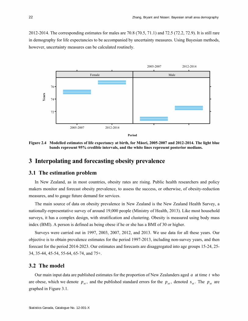
2012-2014. The corresponding estimates for males are 70.8 (70.5, 71.1) and 72.5 (72.2, 72.9). It is still rare
in demography for life expectancies to be accompanied by uncertainty measures. Using Bayesian methods,
however, uncertainty measures can be calculated routinely.
Figure 2.4 Modelled estimates of life expectancy at birth, for Māori, 2005-2007 and 2012-2014. The light blue bands represent 95% credible intervals, and the white lines represent posterior medians.
3 Interpolating and forecasting obesity prevalence
3.1 The estimation problem
In New Zealand, as in most countries, obesity rates are rising. Public health researchers and policy
makers monitor and forecast obesity prevalence, to assess the success, or otherwise, of obesity-reduction
measures, and to gauge future demand for services.
The main source of data on obesity prevalence in New Zealand is the New Zealand Health Survey, a
nationally-representative survey of around 19,000 people (Ministry of Health, 2013). Like most household
surveys, it has a complex design, with stratification and clustering. Obesity is measured using body mass
index (BMI). A person is defined as being obese if he or she has a BMI of 30 or higher.
Surveys were carried out in 1997, 2003, 2007, 2012, and 2013. We use data for all these years. Our
objective is to obtain prevalence estimates for the period 1997-2013, including non-survey years, and then
forecast for the period 2014-2023. Our estimates and forecasts are disaggregated into age groups 15-24, 25-
34, 35-44, 45-54, 55-64, 65-74, and 75+.
3.2 The model
Our main input data are published estimates for the proportion of New Zealanders aged a at time t who
are obese, which we denote ,atp and the published standard errors for the ,atp denoted .ats The atp are
graphed in Figure 3.1.
Yea
rs
2005-2007 2012-2014
Period
76
74
72
2005-2007 2012-2014
Female Male

Survey Methodology, 2019 (special issue) 23
Statistics Canada, Catalogue No. 12-001-X
Figure 3.1 Proportion of obesity in New Zealand, by age and year, as estimated in the New Zealand Health Survey.
When individual-level data are available, the standard Bayesian approach towards accounting for
complex survey design is to include as many features of the design as possible in the estimation model
(Gelman et al., 2014, Chapter 8). Chen, Wakefield and Lumely (2014) show, however, how the full
individual-level approach can be approximated by an aggregate-level approach that starts from design based
estimates such as atp and .ats Chen et al. (2014) assume that the design-based estimates are constructed so
as to reflect all the important features of the survey design, and show how these estimates can be converted
into a form suitable for inclusion in an aggregate-level model.
Applying the approach of Chen et al. (2014), we approximate the individual-level approach using a
Binomial likelihood. We obtain counts of individuals with obesity aty and total counts of individuals atn
by finding aty and atn such that at
at
yatn p and 21 .at at
at at
y yatn n s The likelihood is
Binomial , .at at aty n (3.1)
Here at is the super-population probability of obesity: the probability that a person aged a at time t is
obese. Our objective is to estimate at for past years, including years without survey data, and to forecast
at for future years.
Our prior model for at is
0 age timelogit = ,at a t (3.2)
which includes age and time effects, but not an age-time interaction. We experimented with an age-time
interaction, but found that its size was small enough to omit (results not shown).
As with the mortality model of Section 2, we use a local trend model for the age effect, though in the
obesity case we do not have an infant covariate. The rationale for using a local trend model is, once again,
to capture the correlations between neighbouring age groups. We also use the same prior for the intercept
as we do in Section 2, a normal distribution with mean 0 and standard deviation 10.
We use a local trend model for time,
time time time=t t tu (3.3)
time timetime time1 1=t t t tv (3.4)
timetime time1= ,t t tw (3.5)
Per
cen
t
20 30 40 50 60 70 80 20 30 40 50 60 70 80 20 30 40 50 60 70 80
Age
35
30
25
20
15
10
20 30 40 50 60 70 80 20 30 40 50 60 70 80
1997 2003 2007 2012 2013
24 Zhang, Bryant and Nissen: Bayesian small area demography
Statistics Canada, Catalogue No. 12-001-X
but with two different sets of assumptions about innovation terms timetv and time .tw
In our first version, we assume that timetv and time
tw are always very close to 0, which we implement by
using extremely tight priors on the standard deviations for these terms. The standard deviations for both
terms have half t priors with scales of 0.001. This version of the local trend model essentially fits a
straight line through the data. Aside from assuming no change, this is perhaps the most common approach
to forecasting future rates in epidemiology and demography. We refer to this model as the “straight line”
model.
Our second version is a generalization of the first. Rather than assuming that timetv and time
tw are always
close to 0, we allow them to take values that imply year-on-year changes in obesity rates of a few percentage
points. We do this by setting the scale of the prior for the standard deviation of timetv to 0.05 and setting the
scale of the prior for standard deviation of timetw to 0.025. We use a larger scale for time
tv than for timetw on
the basis that levels change more rapidly than systematic trends. We refer to the model based on this version
of the time effect as the “flexible” model.
We carry out the estimation using our package demest, with the same settings for burnin, production,
chains, and thinning as for the mortality application.
3.3 Results
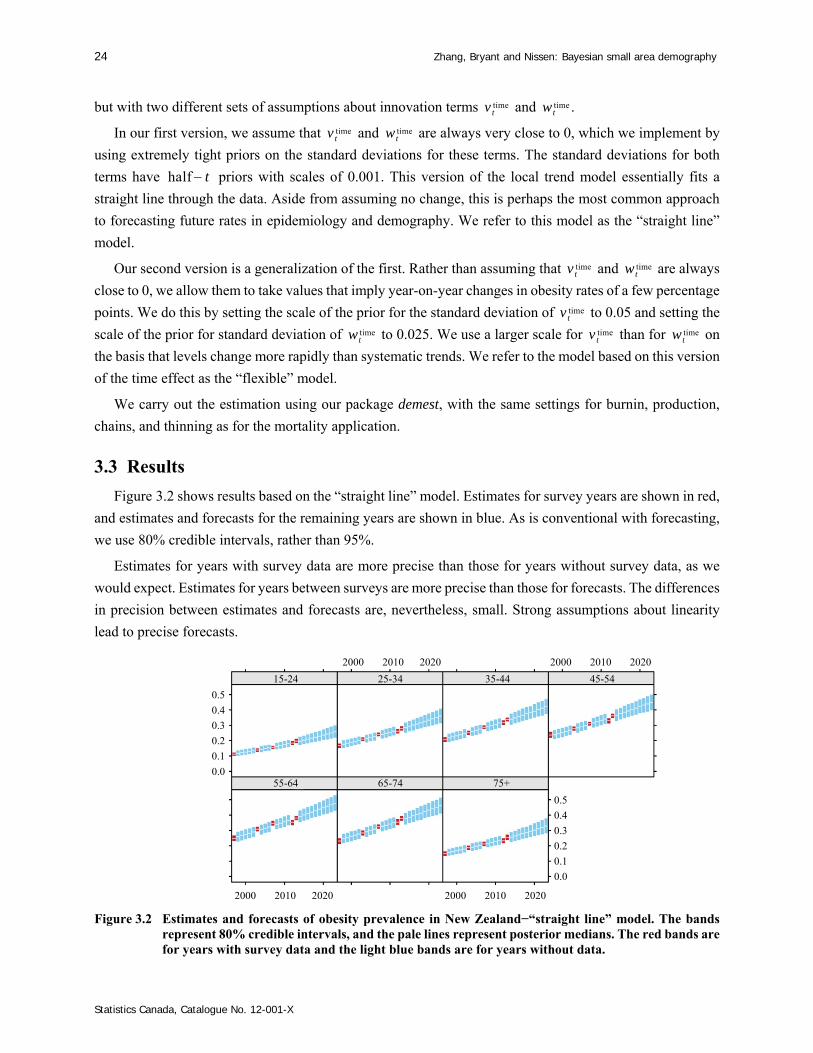
Figure 3.2 shows results based on the “straight line” model. Estimates for survey years are shown in red,
and estimates and forecasts for the remaining years are shown in blue. As is conventional with forecasting,
we use 80% credible intervals, rather than 95%.
Estimates for years with survey data are more precise than those for years without survey data, as we
would expect. Estimates for years between surveys are more precise than those for forecasts. The differences
in precision between estimates and forecasts are, nevertheless, small. Strong assumptions about linearity
lead to precise forecasts.
Figure 3.2 Estimates and forecasts of obesity prevalence in New Zealand−“straight line” model. The bands represent 80% credible intervals, and the pale lines represent posterior medians. The red bands are for years with survey data and the light blue bands are for years without data.
2000 2010 2020 2000 2010 2020
0.5
0.4
0.3
0.2
0.1
0.0
0.5
0.4
0.3
0.2
0.1
0.0
2000 2010 2020 2000 2010 2020
15-24 25-34 35-44 45-54
55-64 65-74 75+
Survey Methodology, 2019 (special issue) 25
Statistics Canada, Catalogue No. 12-001-X
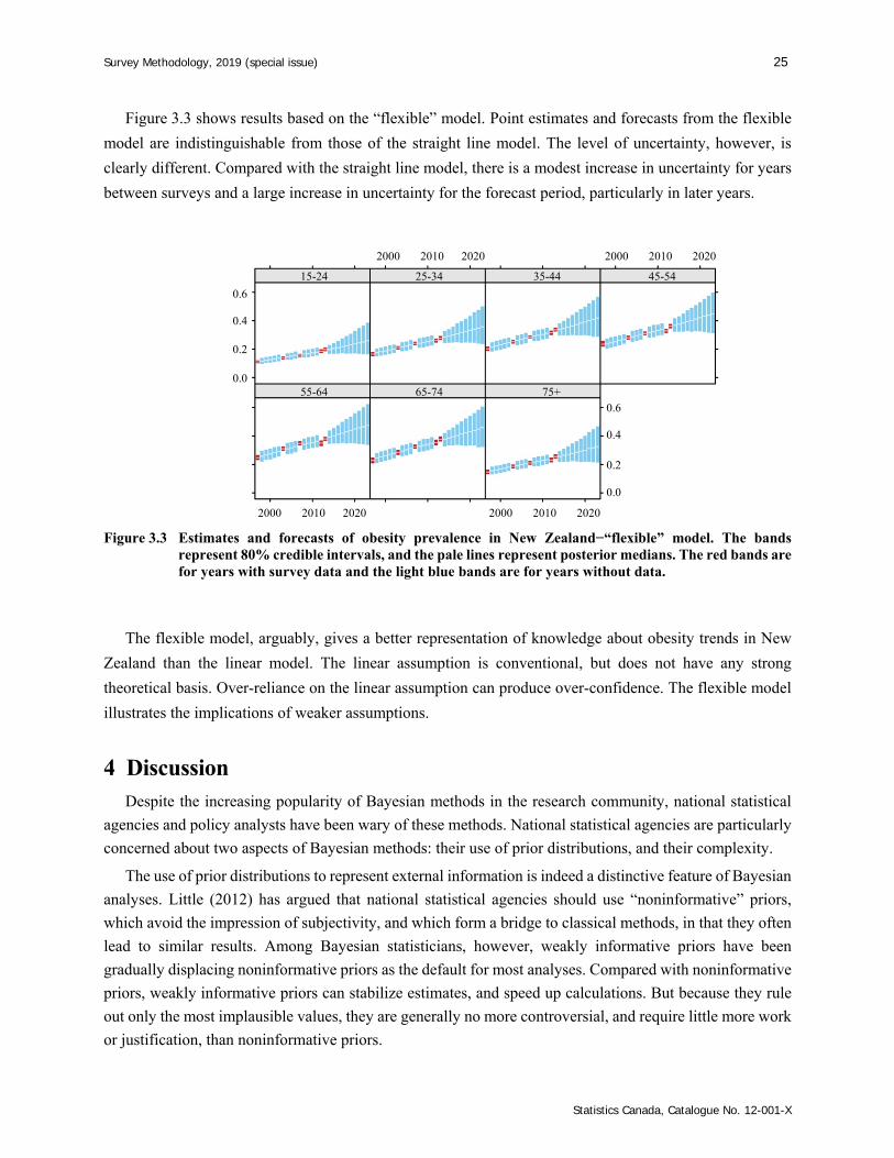
Figure 3.3 shows results based on the “flexible” model. Point estimates and forecasts from the flexible
model are indistinguishable from those of the straight line model. The level of uncertainty, however, is
clearly different. Compared with the straight line model, there is a modest increase in uncertainty for years
between surveys and a large increase in uncertainty for the forecast period, particularly in later years.
Figure 3.3 Estimates and forecasts of obesity prevalence in New Zealand−“flexible” model. The bands represent 80% credible intervals, and the pale lines represent posterior medians. The red bands are for years with survey data and the light blue bands are for years without data.
The flexible model, arguably, gives a better representation of knowledge about obesity trends in New
Zealand than the linear model. The linear assumption is conventional, but does not have any strong
theoretical basis. Over-reliance on the linear assumption can produce over-confidence. The flexible model
illustrates the implications of weaker assumptions.
4 Discussion
Despite the increasing popularity of Bayesian methods in the research community, national statistical
agencies and policy analysts have been wary of these methods. National statistical agencies are particularly
concerned about two aspects of Bayesian methods: their use of prior distributions, and their complexity.
The use of prior distributions to represent external information is indeed a distinctive feature of Bayesian
analyses. Little (2012) has argued that national statistical agencies should use “noninformative” priors,
which avoid the impression of subjectivity, and which form a bridge to classical methods, in that they often
lead to similar results. Among Bayesian statisticians, however, weakly informative priors have been
gradually displacing noninformative priors as the default for most analyses. Compared with noninformative
priors, weakly informative priors can stabilize estimates, and speed up calculations. But because they rule
out only the most implausible values, they are generally no more controversial, and require little more work
or justification, than noninformative priors.
0.6
0.4
0.2
0.0
2000 2010 2020 2000 2010 2020
0.6
0.4
0.2
0.0
2000 2010 2020 2000 2010 2020
15-24 25-34 35-44 45-54
55-64 65-74 75+

26 Zhang, Bryant and Nissen: Bayesian small area demography
Statistics Canada, Catalogue No. 12-001-X
However, in cases where the data to hand do not permit sufficiently strong answers to the questions of
interest, there may be advantages to using priors that are strongly, rather than weakly, informative. In our
obesity example, for instance, it may be possible to improve on both of our forecasting models by specifying
priors for the standard deviation parameters that accurately reflect likely year-on-year variation in obesity
rates.
If statistical agencies were to use strongly informative priors, they would need to spell these priors out
clearly, justify their choices, and test sensitivity to alternative choices. But, in most cases, this would be an
improvement on current practice. Current practice with analyses such as population forecasts is often to
apply informal adjustments, or to retrospectively adjust assumptions, until a plausible result is obtained.
Bayesian methods provide analysts with a more transparent and systematic way of bringing in external
information and expert judgement.
Objections about Bayesian models being complicated are partly true. Many Bayesian models are
complicated, in that, like the models presented in this paper, they use many layers and many parameters. At
the same time, however, the individual components of these models are often simple and intuitive. To make
sense of our model for mortality rates, for instance, we can start with the likelihood, move on to the prior
model, and then consider the priors for main effects and interactions one by one. With this divide-and-
conquer approach, even complicated models are accessible. Moreover, the main assumptions behind the
models can often be described in nontechnical language, even if the mathematical techniques cannot.
Similarly, the traditional objection that Bayesian modelling require advanced computing skills is
gradually losing force. Packages such as ours allow analysts to fit specific classes of demographic estimation
models relatively easily. General-purpose Bayesian programming languages such as Stan (Carpenter,
Gelman, Hoffman, Lee, Goodrich, Betancourt, Brubaker, Guo, Li and Riddell, 2016) offer greater flexibility
in exchange for slightly more programming effort. These tools allow practitioners to easily fit complicated
Bayesian models.
Acknowledgements
The views expressed are those of the authors, and should not be attributed to Peking University, Stats NZ,
or any other organization.
Appendix A
Identification of our model
In the prior model, each main effect or interaction includes all possible categories of the classifying
dimensions. For instance, the sex effect includes separate female and male effects, and the age-sex
interaction includes effects for every possible combination of age and sex. Because all of our priors are
proper (i.e., are genuine probability distributions that integrate to 1), the posterior distribution is proper. All
parameters are therefore identified in the broadest sense, and a Bayesian analysis can be carried out.
The main effects and interactions are, however, only weakly identified. For instance, adding a value
to the female and male effects sexFemale and sex
Male , and subtracting from the intercept 0 , will produce
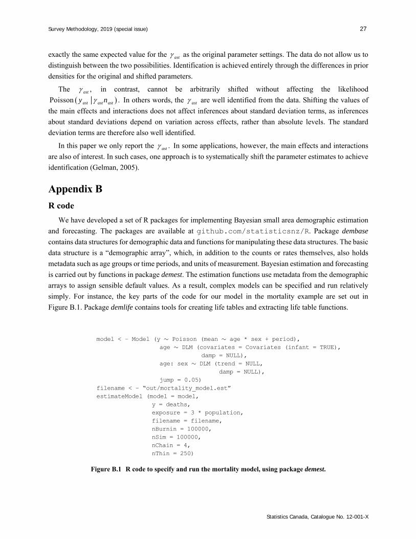
Survey Methodology, 2019 (special issue) 27
Statistics Canada, Catalogue No. 12-001-X
exactly the same expected value for the ast as the original parameter settings. The data do not allow us to
distinguish between the two possibilities. Identification is achieved entirely through the differences in prior
densities for the original and shifted parameters.
The ,ast in contrast, cannot be arbitrarily shifted without affecting the likelihood
Poisson .ast ast asty n In others words, the ast are well identified from the data. Shifting the values of
the main effects and interactions does not affect inferences about standard deviation terms, as inferences
about standard deviations depend on variation across effects, rather than absolute levels. The standard
deviation terms are therefore also well identified.
In this paper we only report the .ast In some applications, however, the main effects and interactions
are also of interest. In such cases, one approach is to systematically shift the parameter estimates to achieve
identification (Gelman, 2005).
Appendix B
R code
We have developed a set of R packages for implementing Bayesian small area demographic estimation
and forecasting. The packages are available at github.com/statisticsnz/R. Package dembase
contains data structures for demographic data and functions for manipulating these data structures. The basic
data structure is a “demographic array”, which, in addition to the counts or rates themselves, also holds
metadata such as age groups or time periods, and units of measurement. Bayesian estimation and forecasting
is carried out by functions in package demest. The estimation functions use metadata from the demographic
arrays to assign sensible default values. As a result, complex models can be specified and run relatively
simply. For instance, the key parts of the code for our model in the mortality example are set out in
Figure B.1. Package demlife contains tools for creating life tables and extracting life table functions.
model < − Model (y ~ Poisson (mean ~ age * sex + period), age ~ DLM (covariates = Covariates (infant = TRUE), damp = NULL), age: sex ~ DLM (trend = NULL, damp = NULL), jump = 0.05)
filename < − “out/mortality_model.est” estimateModel (model = model, y = deaths, exposure = 3 * population, filename = filename, nBurnin = 100000, nSim = 100000, nChain = 4, nThin = 250)
Figure B.1 R code to specify and run the mortality model, using package demest.
28 Zhang, Bryant and Nissen: Bayesian small area demography
Statistics Canada, Catalogue No. 12-001-X
References
Alho, J., and Spencer, B. (2006). Statistical Demography and Forecasting. Springer Science & Business Media.
Bijak, J., and Bryant, J. (2016). Bayesian demography 250 years after Bayes. Population Studies, 70, 1, 1-19.
Bryant, J., and Howard, A. (2017). Estimating Infant Mortality by Ethnicity: New Methods for Dealing with Inconsistent Ethnic Reporting and Small Numbers. Statistics New Zealand, Working Paper No. 17-01.
Bryant, J., Dunstan, K., Graham, P., Matheson-Dunning, N., Shrosbree, E. and Speirs, R. (2016). Measuring Uncertainty in the 2013-Base Estimated Resident Population. Statistics New Zealand, Working Paper No. 16-04.
Carpenter, B., Gelman, A., Hoffman, M., Lee, D., Goodrich, B., Betancourt, M., Brubaker, M.A., Guo, J., Li, P. and Riddell, A. (2016). Stan: A probabilistic programming language. Journal of Statistical Software, 20, 1-37.
Chen, C., Wakefield, J. and Lumely, T. (2014). The use of sampling weights in bayesian hierarchical models for small area estimation. Spatial and Spatio-Temporal Epidemiology, 11, 33-43.
Gelman, A. (2005). Analysis of variance why it is more important than ever (with discussion). The Annals of Statistics, 33, 1, 1-53.
Gelman, A., Jakulin, A., Pittau, M.G. and Su, Y.-S. (2008). A weakly informative default prior distribution for logistic and other regression models. The Annals of Applied Statistics, 2, 4, 1360-1383.
Gelman, A., Carlin, J.B., Stern, H.S., Dunson, D.B., Vehtari, A. and Rubin, D.B. (2014). Bayesian Data Analysis, Third Edition. Boca Raton: Chapman and Hall/CRC.
Gerland, P., Raftery, A.E., Ševčíková, H., Li, N., Gu, D., Spoorenberg, T., Alkema, L., Fosdick, B.K., Chunn, J., Lalic, N., Bay, G., Buettner, T., Heilig, G.K. and Wilmoth, J. (2014). World population stabilization unlikely this century. Science, 346, 6206, 234-237.
Little, R.J. (2012). Calibrated Bayes, an alternative inferential paradigm for official statistics. Journal of Official Statistics, 28, 3, 309.
Ministry of Health (2013). New Zealand health survey: Annual update of key findings 2012/13. Technical report, Ministry of Health.
Pfeffermann, D. (2013). New important developments in small area estimation. Statistical Science, 28, 1, 40-68.
Prado, R., and West, M. (2010). Time Series: Modeling, Computation, and Inference. Boca Raton: Chapman and Hall/CRC.
Preston, S., Heuveline, P. and Guillot, M. (2001). Demography: Modelling and Measuring Population Processes. Blackwell, Oxford.
Rao, J.N.K., and Molina, I. (2015). Small Area Estimation, Second Edition. New York: John Wiley & Sons, Inc.

Survey Methodology, 2019 (special issue) 29
Statistics Canada, Catalogue No. 12-001-X
United Nations General Assembly (2015). Transforming our world: The 2030 agenda for sustainable development. Available at https://www.unfpa.org/resources/transforming-our-world-2030-agenda-sustainable-development.
Vaupel, J.W., Manton, K.G. and Stallard, E. (1979). The impact of heterogeneity in individual frailty on the
dynamics of mortality. Demography, 16, 3, 439-454.


Survey Methodology, 2019 (special issue) 31 Vol. 45, No. 1, pp. 31-59 Statistics Canada, Catalogue No. 12-001-X
1. Hukum Chandra, Indian Agricultural Statistics Research Institute, Library Avenue, New Delhi, India. E-mail: [email protected]; Ray
Chambers, University of Wollongong, Australia; Nicola Salvati, University of Pisa, Italy.
Small area estimation of survey weighted counts under aggregated level spatial model
Hukum Chandra, Ray Chambers and Nicola Salvati1
Abstract
The empirical predictor under an area level version of the generalized linear mixed model (GLMM) is extensively used in small area estimation (SAE) for counts. However, this approach does not use the sampling weights or clustering information that are essential for valid inference given the informative samples produced by modern complex survey designs. This paper describes an SAE method that incorporates this sampling information when estimating small area proportions or counts under an area level version of the GLMM. The approach is further extended under a spatial dependent version of the GLMM (SGLMM). The mean squared error (MSE) estimation for this method is also discussed. This SAE method is then applied to estimate the extent of household poverty in different districts of the rural part of the state of Uttar Pradesh in India by linking data from the 2011-12 Household Consumer Expenditure Survey collected by the National Sample Survey Office (NSSO) of India, and the 2011 Indian Population Census. Results from this application indicate a substantial gain in precision for the new methods compared to the direct survey estimates.
Key Words: Complex surveys; Direct survey weighted estimator; Poverty estimate; Spatial Model; Mapping.
1 Introduction
Sample surveys are generally planned to produce estimates for population characteristics of interest
mainly at higher geographic (e.g., national and state) levels. The sample size is fixed in such a way that the
direct estimators for larger domains provide reliable estimates, where by direct estimators we mean
estimators that use only sample-weighted data from the domain of interest. In many practical situations,
however, the aim is to estimate parameters for domains that contain only a small number of sample
observations. The term “small areas” is used to describe domains whose sample sizes are not large enough
to allow sufficiently precise direct estimation. When direct estimation is not possible, one has to rely on
alternative, model-based methods for producing small area estimates. Such methods depend on model
specification as well as on the availability of population level auxiliary information related to the variable
of interest, and are commonly referred to as indirect methods (Rao, 2003). The underlying theory is referred
to as the small area estimation (SAE), and SAE techniques aim at producing reliable estimates based on
such small sample sizes by using the model “linking” the small areas to “borrow strength” from the sample
data from other small areas, see for example, Pfeffermann (2002) and Rao and Molina (2015). In this
context, we differentiate between SAE methods based on unit-level models and those based on area-level
models. In the former case these models are for the individual survey measurements and include area effects,
while in the latter case these models are used to smooth out the variability in the unstable area-level direct
survey estimates. Area-level modelling is typically used when unit-level data are unavailable, or, as is often
the case, where model covariates (e.g., census variables) are only available at area level. The Fay-Herriot
model (Fay and Herriot, 1979), is a widely used area level model that assumes area-specific survey estimates
32 Chandra, Chambers and Salvati: Small area estimation of survey weighted counts under aggregated level spatial model
Statistics Canada, Catalogue No. 12-001-X
are available, and that these follow an area level linear mixed model with independent area random effects.
This model can also accommodate survey weights in SAE by using the survey weighted direct estimates
when fitting the linear mixed model. When the variable of interest is not continuous (for example, binary
and count data), a generalized linear mixed model (GLMM) is often used. If the variable of interest is binary
and the target of inference is a small area proportion, then the GLMM with logistic link function (also
referred as the logistic linear mixed model) is commonly used. An empirical plug-in predictor (EP) is
commonly used for the estimation of small area proportions under a GLMM, see for example, Chandra,
Chambers and Salvati (2012), Salvati, Chandra and Chambers (2012), Rao and Molina (2015) and
references therein, although it is not the most efficient predictor under this model. An alternative is the
Empirical Best Predictor (EBP, Jiang, 2003). This predictor does not have a closed form in general and so
must be computed via numerical approximation, which is typically not straightforward. As a consequence
national statistical agencies tend to favour computation of an approximation like the EP. It is also our
understanding that EP-type predictors are used in Molina, Saei and José Lombardìa (2007) and Lopez-
Vizcaino, Lombardìa and Morales (2013). When only area level data are available, an area level version of
a GLMM can be considered for SAE, see for example, Saei and Chambers (2003), Johnson, Chandra, Brown
and Padmadas (2010), Chandra, Salvati and Sud (2011), Chandra, Salvati and Chambers (2017) and
references therein. Unlike the Fay-Herriot model, this approach implicitly assumes simple random sampling
with replacement within each area and ignores the survey weights. Unfortunately, this has the potential to
seriously bias the estimates if the small area samples are seriously unbalanced with respect to key population
charcteristics. Consequently use of the survey weights appears to be inevitable for if one wishes to generate
representative small area estimates.
Modelling the survey weighted estimates of proportions by a continuous distribution, as in the Fay-
Herriot model, can be problematic since the sampling distribution of these proportions is inherently discrete
due to small sample sizes and binary nature of the underlying observations. For example, such a linear model
based approach can lead to negative predictions or, more likely, prediction intervals that include negative
values, both absurd results. Clearly GLMMs are more suitable for modelling inherently discrete data arising
from survey weighted direct estimates, see Liu, Lahiri and Kalton (2014), Ghosh, Natarajan, Stroud and
Carlin (1998) and Rao (2003, Sections 5.6 and 10.11). Malec, Sedransk, Moriarity and LeClere (1997)
describe a hierarchical Bayes model for binary survey data. The authors examined the use of sampling
weights as a covariate in the model and did not find any improvement for their example of county-level data
from the National Health Interview Survey. Unlike estimation of survey weighted linear parameters like
small area means and totals, there has been comparatively little research on estimation of survey weighted
small area proportions or counts under area level small area models. Recently, some authors including
Mercer, Wakefield, Chen and Lumley (2014), Liu et al. (2014) and Franco and Bell (2013) have described
how survey weights can be used in a Bayesian hierarchical model framework for estimating small area
proportions by using effective sample sizes for inference about the underlying binomial distributions in
order to preserve sampling variances estimated via a generalized variance function. These approaches are
defined within a Bayesian framework. In this article, we adopt a frequentist approach and describe an SAE
Survey Methodology, 2019 (special issue) 33
Statistics Canada, Catalogue No. 12-001-X
method that uses the sampling weights for binary data when estimating small area proportions under an area
level version of a GLMM. Following Korn and Graubard (1998), we model the survey weighted estimates
as binomial proportions, with an “effective sample size” chosen to match the binomial variance to the
sampling variance of the estimates. Using the effective sample size rather than the actual sample size allows
for the varying information in each area under complex sampling. Furthermore, the area-specific random
effects in the GLMM are typically assumed to be independent, that is, different small areas are considered
to be independent of each other. However, in practice most small area boundaries are arbitrary and there
appears to be no good reason why units that are just one side of such a boundary should not generally be
correlated with units just on the other side (Pratesi and Salvati, 2008). One approach to incorporating such
spatial information in SAE modelling is to extend the random effects model to allow for spatially correlated
area effects using, for example, a Simultaneous Autoregressive (SAR) model. See Anselin (1992) and
Cressie (1993). These models embed spatial behaviour in the model random effects, which in the context of
SAE typically means area effects. Applications of SAR models in small area estimation have been
considered by Singh, Shukla and Kundu (2005), Pratesi and Salvati (2008), Pratesi and Salvati (2009),
Molina, Salvati, and Pratesi (2009), Marhuenda, Molina and Morales (2013) and Porter, Wikle and Holan
(2015). SAR models are commonly used for modelling spatial dependence under the frequentist approach
to SAE. Other the hand, Bayesian approaches to SAE favour Conditionally Auto-Regressive (CAR) models
for modelling spatial dependence, see Besag, York and Mollié (1991), Leroux, Lei and Breslow (1999) and
Mercer et al. (2014). This paper takes a frequentist approach to SAE and so we consider an extension of an
area level GLMM to account for spatial dependence between the small areas based on a SAR specification,
and develop small area estimates under this model that use the survey design information.
The structure of the paper is as follows. Section 2 describes the data from the 2011-12 Household
Consumer Expenditure Survey of the National Sample Survey Office (NSSO) of India and the 2011 Indian
Population Census that will be used to estimate the district level incidence of household poverty in the rural
part of the Indian State of Uttar Pradesh. In Section 3 we set out the theoretical background to the area level
version of the GLMM, and then discuss the use of effective sample size for incorporating the information
in the survey weights when estimating small area proportions under this model. The spatial extension of the
area level GLMM, as well as an empirical predictor based on this model, are also introduced in this section.
The results from the poverty incidence application along with various diagnostic measures are reported in
Section 4. In this section we also provide a poverty map that serves to demonstrate district-level inequalities
in the distribution of poor rural households in Uttar Pradesh. Finally, Section 5 summarizes the paper and
provides concluding remarks.
2 Data description
This section introduces the basic sources of the data, i.e., the 2011-12 Household Consumer Expenditure
Survey (HCES) of the NSSO for rural areas of the State of Uttar Pradesh in India and the 2011 Population
Census, used in the small area application reported in this paper. Data obtained from these sources are then

34 Chandra, Chambers and Salvati: Small area estimation of survey weighted counts under aggregated level spatial model
Statistics Canada, Catalogue No. 12-001-X
used to estimate the proportion of poor households at district level in Uttar Pradesh. The State of Uttar
Pradesh is the most populous State in the country and accounts for about 16.16 per cent of India’s
population. It covers 243,290 square km, equal to 6.88% of the total area of the country. Poverty estimates
in India are produced for all the States separately for both rural and urban sectors. Our analysis is restricted
to the rural areas of Uttar Pradesh because about 78% of the population of this State live in rural areas
according to 2011 Population Census. The NSSO conducts nationwide HCE surveys at regular intervals as
part of its “rounds”, with the duration of each round normally being a year. These surveys are aimed at
generating estimates of average household monthly per capita consumer expenditure (MPCE), the
distribution of households and persons over the MPCE range, and the break-up of average MPCE by
commodity group, separately for the rural and urban sectors of the country, for States and Union Territories,
and for different socio-economic groups. These indicators are amongst the most important measures of the
living conditions of the relevant domains of the population. The surveys are conducted through interviews
of a representative sample of households selected randomly through a suitable sampling design and covering
almost the entire geographical area of the country. In particular, the sampling design used in the NSSO
survey is stratified multi-stage random sampling with districts as strata, villages as first stage units and
households as second stage units. Although, these surveys provide reliable and representative state and
national level estimates, they cannot be used directly to produce reliable estimates at the district level due
to small sample sizes. In particular, although district is a very important domain of the planning process in
India, there are no surveys aimed at producing estimates at this level. The lack of robust and reliable outcome
measures at the district level puts constraints on the design of targeted interventions and policy development.
More importantly, state and national estimates do not adequately capture the extent of geographical
inequalities, which restricts the scope for evaluating progress locally within and between districts. Balanced
against all of this however is the fact that conducting a district level survey would be very costly as well as
time-consuming. In the 2011-12 HCES, a total of 5,916 households from the 71 districts of Uttar Pradesh
were surveyed. The district sample sizes ranged from 32 to 128 with average of 83. It is evident that these
district level sample sizes are relatively small, with an average sampling fraction of 0.0002. As a
consequence, it is difficult to generate reliable district level direct survey estimates with associated standard
errors from this survey. This small sample size problem can be resolved by using SAE methodology
provided auxiliary information is available to strengthen the limited sample data from the districts (Rao and
Molina, 2015; Tzavidis, Salvati, Pratesi and Chambers, 2008).
We note here that the target variable Y at the unit (household) level in the published survey data file is
binary, corresponding to whether a household is poor or not. In our application however we focus on
estimation where the available data are the corresponding counts of the number of poor households in
sample in each district. In this context a household having MPCE below the state poverty line is defined as
being poor. The poverty line used in this study (Rs. 768) is the same as that set by the Planning Commission,
Govt. of India, for 2011-12. The parameter of interest is then the proportion of poor rural households within
each district. The auxiliary variables (covariates) used in our analysis are taken from the Indian Population
Census of 2011. These auxiliary variables are only available as counts at district level, and so SAE methods
Survey Methodology, 2019 (special issue) 35
Statistics Canada, Catalogue No. 12-001-X
based on area level small area models, as described in next section, must be employed to derive the small
area estimates. There are approximately 50 such covariates that are available for use in SAE analysis. We
therefore carried out a preliminary data analysis in order to define appropriate covariates for SAE modelling,
using Principal Component Analysis (PCA) to derive composite scores for selected groups of variables. In
particular, we carried out PCA separately on three groups of variables, all measured at district level and
identified as S1, S2 and S3 below. The first group (S1) consisted of literacy rates by gender and proportions
of worker population by gender. The first principal component (S11) for this group explained 51% of the
variability in the S1 group, while adding the second principal component (S12) increased explained
variability to 85%. The second group (S2) consisted of the proportions of main worker by gender,
proportions of main cultivator by gender and proportions of main agricultural labourer by gender. The first
principal component (S21) for this second group explained 49% of the variability in the S2 group, while
adding the second component (S32) increased explained variability to 67%. Finally, the third group (S3)
consisted of proportions of marginal cultivator by gender and proportions of marginal agriculture labourers
by gender. The first principal component (S31) for this third group explained 61% of the variability in the
S3 group, while adding the second component (S22) increased explained variability to 78%. Using the
methods detailed in the following sections, we fitted a generalised linear model using direct survey estimates
of proportions of poor rural households as the response variable and the six principal component scores S11,
S12, S21, S22, S31 and S32 as potential covariates. The final selected model included the three covariates
S11, S21 and S31, with residual deviance and AIC values of 327.18 and 636.89, respectively. This final
model was then used to produce district wise estimates of rural poverty incidence, i.e., estimates of the head
count ratio (HCR) at this level.
A major problem with application of SAE in many developing and underdeveloped countries is the fact
that administrative or civic registration data that are suitable for use as covariates in the SAE model are
unavailable at small area level. Typically, what auxiliary variables are available (e.g., census tabulations)
do not have good association with variable of interest. This results in very limited information for producing
the small area estimates. In such cases, it can be beneficial to supplement the available data by using
geospatial information about the small areas. In this study, we use the geographical locations (centroids) of
the different districts in the Indian State of Uttar Pradesh to extend our SAE model to one that allows rural
poverty counts from neighbouring districts to be correlated.
3 Small area estimation under the area level GLMM
3.1 Spatially uncorrelated random area effects
We assume that a probability sampling method is used to draw a sample s of size n from a finite
population U of size ,N which consists of D non-overlapping domains 1, , .iU i D Following
standard practice, we refer to these domains as small areas or just areas. Furthermore, we assume that there
is a known number iN of population units in small area ,i with in of these sampled. The total number of

36 Chandra, Chambers and Salvati: Small area estimation of survey weighted counts under aggregated level spatial model
Statistics Canada, Catalogue No. 12-001-X
units in the population is 1
,D
iiN N
with corresponding total sample size
1.
D
iin n
We use s to
denote the collection of units in sample, with is the subset drawn from small area i (i.e., | | ),i is n and
use expressions like j i and j s to refer to the units making up small area i and sample ,s
respectively. Similarly, ir denotes the set of units in small area i that are not in sample, with | |i i ir N n
and .i i iU s r Let ijy denotes the value of the variable of interest for unit j 1, , ij N in area .i
The variable of interest, with values ,ijy is binary (e.g., 1ijy if household j in area i is poor household
and 0 otherwise), and the aim is to estimate the small area population count, ,i
i ijj Uy y
or equivalently
the small area proportion, 1 ,i
i i ijj UP N y
in area i 1, , .i D The standard direct survey
estimator (hereafter denoted by DIR) for iP is ,i
iw ij ijj sp w y
where
iij ij ijj s
w w w
is the
normalized survey weight for unit j in area i with 1i
ijj sw
and ijw is the survey weight for
unit j in area .i The estimated design-based variance of DIR is approximated by iwv p
21 .
iij ij ij iwj s
w w y p
This formula for the variance estimator of DIR is obtained from Särndal,
Swensson and Wretman (1992; see pages 43, 185 and 391), with the simplifications 1 ,ij ijw a ,ij ij ija a
and , , ,ij ik ij ika a a j k where ija is the first order inclusion probability of unit j in area i and ,ij ika is
the second order inclusion probability of units j and k in area .i Under simple random sampling (SRS), 1
ij i iw N n and DIR is then 1 ,i i sip n y with estimated variance 1 1 ,i i i iv p n p p where
isi ijj s
y y
denotes the sample count in area .i
If the sampling design is informative, the SRS-based version of DIR defined in the previous paragraph
may be biased. For the 2011-12 HCES we therefore computed district specific design effects, defined by
the ratios of the variance of the weighted estimates (i.e., for a given sampling design) to the variance of the
unweighted estimates (i.e., assuming SRS). These design effects were more than one in all but three districts,
with values greater than one that varied from 1.17 to 8.44 with an average of 2.71. This is strong evidence
that the sampling design used in the 2011-12 HCES is informative. Furthermore, DIR is based on area-
specific sample data and can therefore be very imprecise when the area specific sample size is small or may
even be impossible to compute if this sample size is zero. However, model-based SAE procedures that
“borrow strength” via a common statistical model for all the small areas can be used to address this problem,
see Rao and Molina (2015).
Suppose now that the available data consist of the sample aggregates siy (i.e., the sample counts of poor
households), together with the values of area specific contextual covariates. That is, for area i we observe
the count siy together with a k -vector of area-specific covariates ix derived from secondary data sources
(e.g., the census or administrative registers). If we ignore the sampling design, the sample count siy in area
i can be assumed to follow a Binomial distribution with parameters in and ,i i.e., Bin , ,si i iy n
where i is the probability of occurrence of an event for a population unit in area i or the probability of
prevalence in area .i Following Saei and Chambers (2003), Johnson et al. (2010) and Chandra et al. (2011),
the model linking the probability i with the covariates ix is the logistic linear mixed model of form
1logit ln 1 ,Ti i i i i iu x β (3.1)

Survey Methodology, 2019 (special issue) 37
Statistics Canada, Catalogue No. 12-001-X
with 1exp 1 exp expit .T T Ti i i i i i iu u u x β x β x β Here β is the k -vector of regression
coefficients, often referred to as the vector of fixed effects, and iu is the area-specific random effect, with
20, .i uu N The model (3.1) is a special case of the generalized linear mixed model (GLMM) with a
logit link function (Breslow and Clayton, 1993). We can observe that the parameters β and 2u are the
same for every area; i.e., they can be estimated using the data from all small areas. This is usually
accomplished by “stacking” the D area level models given by (3.1) to produce a population level model of
the form
η Xβ Zu (3.2)
with 1 , , expit ,TD π η where 1 , , ,T
D η 1 , , TT TDX x x is the D k matrix
of covariates, 1 , , TDZ z z is a matrix of known covariates of dimension D D characterising
differences among the small areas, iz is the D -vector 0, , 1, , 0 T with the 1 in the thi position and
1 , , TDu uu is the D -vector of random area effects with ,Nu 0 Ω where 2
u Ω Ω 2u D I and DI is a D D diagonal matrix.
The Penalized Quasi-Likelihood (PQL) approach is a widely used estimation procedure when fitting a
GLMM. This approach constructs a linear approximation to the non-normal response variable and then
assumes that this linearized dependent variable is approximately normal. The PQL method is widely used
in small area estimation because it is much easier to implement in practice than estimation under the EBP
approach. In particular, we employ a hybrid approach, with PQL used to estimate the parameters β and u
in the GLMM (3.2), and restricted maximum likelihood used to estimate the variance parameter 2 .uΩ
See Breslow and Clayton (1993), Saei and Chambers (2003) and Manteiga, Lombardia, Molina, Morales
and Santamarìa (2007). It is known that in some situations PQL can lead to inconsistent estimators, however
recent empirical applications of PQL (Manteiga et al., 2007) note that the method works well in practice.
Under the model (3.2), the expected values of siy and riy given iu are given by si
expit T Tsi i i i iE y u n x β z u and expit ,T T
ri ri i i i i iE y u N n x β z u respectively.
Under (3.2), a plug-in empirical predictor (EP) of the population count iy in area i is
EP EPˆ ˆˆ ,i si ri si i i iy y y N n (3.3)
where EP ˆˆ ˆexpit .T Ti i i x β z u An estimate of the corresponding proportion in area i is obtained as
EP 1 EPˆ ˆ .i i iP N y For non-sampled area i with associated vector of covariates , out ,ix the synthetic estimator
of iy under (3.2) is SYN SYNˆˆ ,i i iy N with SYN, out
ˆˆ expit .Ti i x β
The model (3.1), being based on unweighted sample counts, assumes that sampling within areas is non-
informative given the values of the contextual variables and the random area effects. As a result, the
predictor (3.3) ignores the complex survey design. If the sampling design is informative and survey
weighted counts are available, there are two main difficulties. First, the values for the weighted sample
counts will not necessarily be the integers 0, 1, , ;in rather they will take a value from a finite set of
unequally-spaced numbers (not necessarily integers) determined by the survey weights of the sample cases
in area .i Second, the estimated sampling variance of the weighted sample counts, siy implied by the
38 Chandra, Chambers and Salvati: Small area estimation of survey weighted counts under aggregated level spatial model
Statistics Canada, Catalogue No. 12-001-X
Binomial distribution, i.e., 1 ,siw i iw iwv y n p p will be incorrect. Korn and Graubard (1998) suggest
that one instead model the survey weighted probability estimate for an area as a binomial proportion, with
an “effective sample size” that equates the resulting binomial variance to the actual sampling variance of
the survey weighted direct estimate for the area. The use of “effective sample size” has been discussed by a
number of authors including Mercer et al. (2014) and Liu et al. (2014) as a way of incorporating the survey
weights. Mercer et al. (2014) observe that the pseudo likelihood approach and effective sample size
approach lead to identical estimates of small area proportions. Using the effective sample size rather the
actual sample size allows for the survey weights under complex sampling. Furthermore, the precision of an
estimate from a complex sample can be higher than for a simple random sample, because of the better use
of population data through a representative sample drawn using a suitable sampling design. Here we use a
subscript of e in all the quantities associated with the “effective sample size”. We address the above two
issues by defining an “effective sample size” ,i en and an “effective sample count” ,is ey such that
.iwis e i ey n p This leads to
is e
i e
y
iw np with its corresponding estimator of variance estimate .iwv p
The model (3.1) is then applied assuming the effective sample count is ey in small area i follows a Binomial
distribution, i.e., Bin , .iis e i ey n The “effective sample size” i en is given by *
ˆ ˆ1,i
i
i
w
P P
i e v pn where
ˆiP is a preliminary model-based prediction of the population proportion iP under a generalised linear
model, and the estimate of variance *iwv p depends on ˆ
iP through a fitted generalized variance function
(GVF), see Liu et al. (2014). Here, 0is ey if 0,iwp but this does not cause problems since ˆ 0iP
implies 0.i en Note that we use a generalised variance function (GVF) to generate estimates of the
sampling variance even for areas that have an observed count of zero. Consequently we do not exclude any
area from model fitting. The empirical predictor of iy is finally obtained by replacing , si in y by
,i e is en y in (3.2), thus ensuring that sampling weights are used in the small area estimation process. In
particular, the plug-in empirical predictor (EP) of iy is then
EP EPˆˆ ,ii e is e i e i ey y N n (3.4)
with EP ˆˆ ˆexpit .T Ti ii e e e x β z u The estimate of the proportion in area i is
EP EP1ˆ ˆ .ii e i eP N y Here ˆ
eβ
and ˆ i eu are the estimates of the fixed effects parameter and the predictor of the random effects parameter
respectively under model (3.2), based on an “effective sample size” ,i en and an “effective sample count”
.is ey Similarly, the synthetic estimator of iy is SYN SYNˆˆ ,ii e i ey N with SYN
, outˆˆ expit .T
ii e e x β
3.2 Computation of effective sample size
Building on the ideas set out in Liu et al. (2014) and Franco and Bell (2013), we describe a procedure
for calculating the district-wise values of effective sample size as well as the corresponding effective sample
count of the number of poor households. We first obtain an approximate model-based prediction of ,iP say ˆ ,iP from a logistic linear model fitted to district-specific direct (i.e., weighted) estimates iwp and a set of
district level auxiliary variables. This model is fitted using the glm function in R, specifying the family as
“binomial” and with the district specific sample sizes as the weights. By definition, these model-based
estimates, ˆˆ exp Ti iP x λ will lie inside the interval (0, 1). Here ix denotes the vector of covariates used
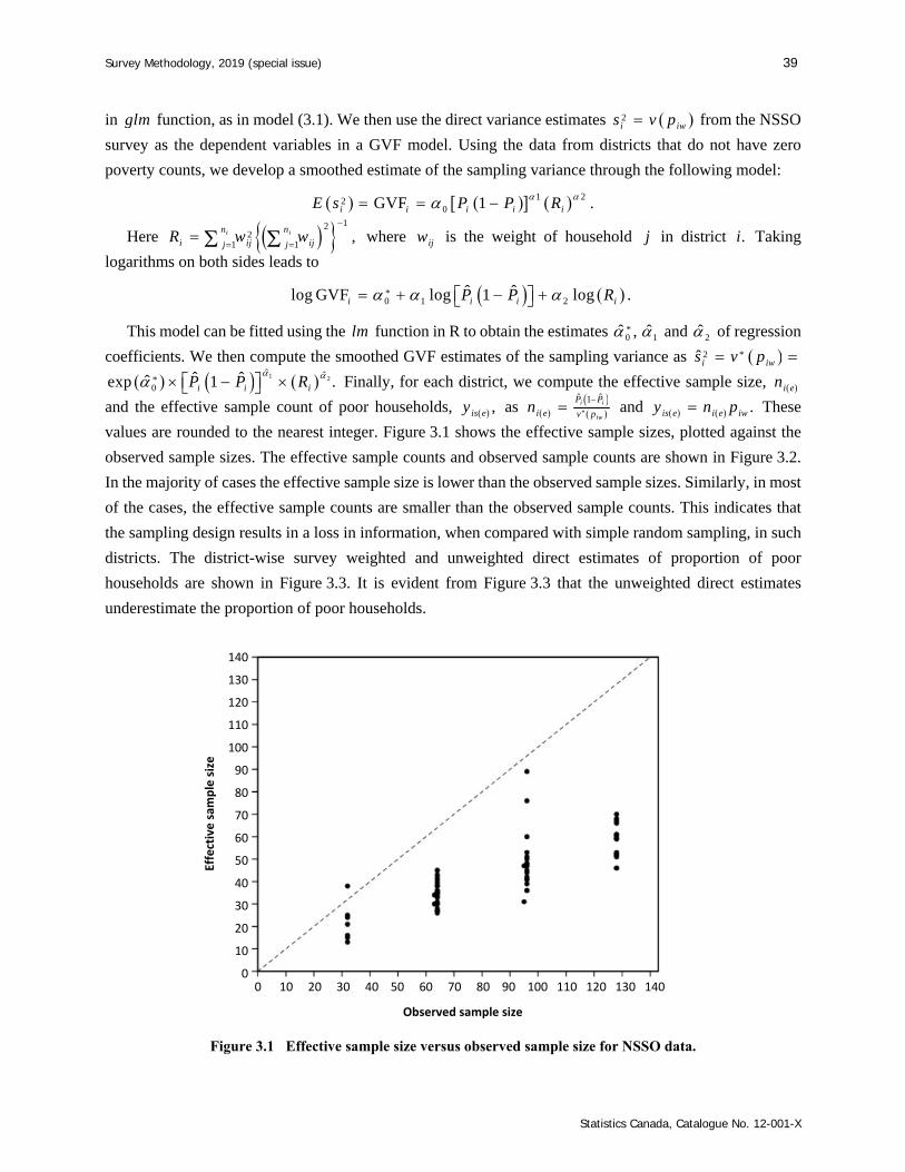
Survey Methodology, 2019 (special issue) 39
Statistics Canada, Catalogue No. 12-001-X
in glm function, as in model (3.1). We then use the direct variance estimates 2i iws v p from the NSSO
survey as the dependent variables in a GVF model. Using the data from districts that do not have zero
poverty counts, we develop a smoothed estimate of the sampling variance through the following model:
1 220GVF 1 .i i i iiE s P P R
Here 122
1 1,i in n
i ij ijj jR w w
where ijw is the weight of household j in district .i Taking
logarithms on both sides leads to
*0 1 2
ˆ ˆlog GVF log 1 log .i iii P P R
This model can be fitted using the lm function in R to obtain the estimates *0ˆ , 1 and 2 of regression
coefficients. We then compute the smoothed GVF estimates of the sampling variance as 2 *ˆi iws v p
1 2ˆ ˆ*
0ˆ ˆˆexp 1 .i i iP P R
Finally, for each district, we compute the effective sample size, i en
and the effective sample count of poor households, ,is ey as *
1ˆ ˆi
w
i
i
P P
i e v pn and .iwis e i ey n p These
values are rounded to the nearest integer. Figure 3.1 shows the effective sample sizes, plotted against the
observed sample sizes. The effective sample counts and observed sample counts are shown in Figure 3.2.
In the majority of cases the effective sample size is lower than the observed sample sizes. Similarly, in most
of the cases, the effective sample counts are smaller than the observed sample counts. This indicates that
the sampling design results in a loss in information, when compared with simple random sampling, in such
districts. The district-wise survey weighted and unweighted direct estimates of proportion of poor
households are shown in Figure 3.3. It is evident from Figure 3.3 that the unweighted direct estimates
underestimate the proportion of poor households.
Figure 3.1 Effective sample size versus observed sample size for NSSO data.
0 10 20 30 40 50 60 70 80 90 100 110 120 130 140
Observed sample size
140
130
120
110
100
90
80
70
60
50
40
30
20
10
0
Effective sam
ple size

40 Chandra, Chambers and Salvati: Small area estimation of survey weighted counts under aggregated level spatial model
Statistics Canada, Catalogue No. 12-001-X
Figure 3.2 Effective sample count versus observed sample count for NSSO data.
Figure 3.3 District-wise survey weighted direct estimates versus unweighted direct estimates of proportion of poor households.
0 5 10 15 20 25 30 35 40 45 50
Observed sample count
50
45
40
35
30
25
20
15
10
5
0
Effective sam
ple count
0.0 0.1 0.2 0.3 0.4 0.5 0.6 0.7 0.8
Unweighted direct estimates
0.8
0.7
0.6
0.5
0.4
0.3
0.2
0.1
0.0
Survey weighted direct estim
ates
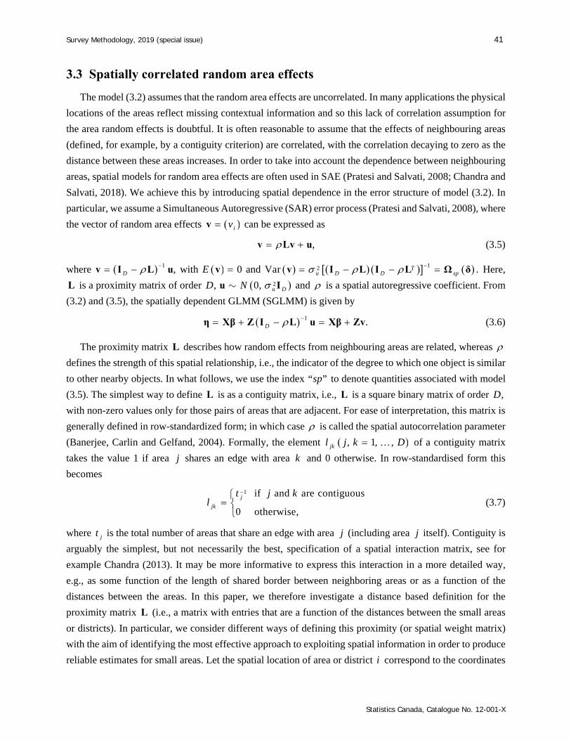
Survey Methodology, 2019 (special issue) 41
Statistics Canada, Catalogue No. 12-001-X
3.3 Spatially correlated random area effects
The model (3.2) assumes that the random area effects are uncorrelated. In many applications the physical
locations of the areas reflect missing contextual information and so this lack of correlation assumption for
the area random effects is doubtful. It is often reasonable to assume that the effects of neighbouring areas
(defined, for example, by a contiguity criterion) are correlated, with the correlation decaying to zero as the
distance between these areas increases. In order to take into account the dependence between neighbouring
areas, spatial models for random area effects are often used in SAE (Pratesi and Salvati, 2008; Chandra and
Salvati, 2018). We achieve this by introducing spatial dependence in the error structure of model (3.2). In
particular, we assume a Simultaneous Autoregressive (SAR) error process (Pratesi and Salvati, 2008), where
the vector of random area effects ivv can be expressed as
, v Lv u (3.5)
where 1 ,D v I L u with 0E v and 12Var .Tu D D sp v I L I L Ω δ Here,
L is a proximity matrix of order ,D 20, u DN u I and is a spatial autoregressive coefficient. From
(3.2) and (3.5), the spatially dependent GLMM (SGLMM) is given by
1 .D η Xβ Z I L u Xβ Zv (3.6)
The proximity matrix L describes how random effects from neighbouring areas are related, whereas
defines the strength of this spatial relationship, i.e., the indicator of the degree to which one object is similar
to other nearby objects. In what follows, we use the index sp“ ” to denote quantities associated with model
(3.5). The simplest way to define L is as a contiguity matrix, i.e., L is a square binary matrix of order ,D
with non-zero values only for those pairs of areas that are adjacent. For ease of interpretation, this matrix is
generally defined in row-standardized form; in which case is called the spatial autocorrelation parameter
(Banerjee, Carlin and Gelfand, 2004). Formally, the element , 1, ,jkl j k D of a contiguity matrix
takes the value 1 if area j shares an edge with area k and 0 otherwise. In row-standardised form this
becomes
1 if and are contiguous
0 otherwise,
j
jk
t j kl
(3.7)
where jt is the total number of areas that share an edge with area j (including area j itself). Contiguity is
arguably the simplest, but not necessarily the best, specification of a spatial interaction matrix, see for
example Chandra (2013). It may be more informative to express this interaction in a more detailed way,
e.g., as some function of the length of shared border between neighboring areas or as a function of the
distances between the areas. In this paper, we therefore investigate a distance based definition for the
proximity matrix L (i.e., a matrix with entries that are a function of the distances between the small areas
or districts). In particular, we consider different ways of defining this proximity (or spatial weight matrix)
with the aim of identifying the most effective approach to exploiting spatial information in order to produce
reliable estimates for small areas. Let the spatial location of area or district i correspond to the coordinates

42 Chandra, Chambers and Salvati: Small area estimation of survey weighted counts under aggregated level spatial model
Statistics Canada, Catalogue No. 12-001-X
of an arbitrarily defined spatial location (i.e., two dimensional x y coordinates or latitude and longitude)
in the area, e.g., its centroid, which we denote by , .i ix iyc c c Let jk j kd c c be an appropriate
measure of the distance between the spatial locations of areas j and .i We then consider the following
specifications for the proximity matrix L as function of distance:
(i) Proximity defined as the inverse of distance between the areas:
1 ;
0 .
jk
jk
d j kl
j k
L (3.8)
(ii) An exponential specification for the proximity function, defined as
2exp 0.5jk jkl d L (3.9)
(iii) A Gaussian specification for the proximity function, defined as
2exp 0.5 ,jk jkl d b L (3.10)
where parameter b is the bandwidth, which can be optimally defined using a least squares
criterion (Fotheringham, Brunsdon and Charlton, 2002). The bandwidth is a measure of how
quickly the proximity decays with increasing distance. We use a cross validation procedure to
estimate bandwidth. Here as the distance between areas j and k increases the proximity in (3.10)
decreases exponentially. In particular, we use the .gwr sel function in the spgwr package of R
to compute the value of the bandwidth. We also use the .Moran I function in the ape package
of R to test for the presence of spatial correlation in the data. The results from this test show that
there is evidence of spatial autocorrelation in the NSSO data. In particular, we reject the null
hypothesis of zero spatial correlation at a 1 per cent level of significance.
In model (3.5), there are 2 parameters 2( u and ) that need to be estimated. Put 2 , .Tu δ
Replacing these unknown parameters by their estimated values 2ˆ ˆˆ , ,Tu δ and denoting subsequent
plug-in estimators by a “hat”, we define the spatial empirical predictor (SEP) of the population count in area
i as
SEP SEPˆˆ ,ii e is e i e i ey y N n (3.11)
with SEP ˆˆ ˆexpit .spT Ti ii e e e x β z v The corresponding spatial empirical predictor of the proportion in
area i is SEP SEP1ˆ ˆ .ii e i eP N y For a non-sampled area, the spatial synthetic empirical predictor (hereafter
denoted by SpSyn) of iP is SpSyn, out
ˆˆ expit .spTii e eP x β Here
ˆ speβ is the estimate of the fixed effect
parameters β and ˆ ev is the predicted value of the spatially correlated random effects v under the SAR
model, using “effective sample size” and “effective sample counts”. The estimation of unknown model
parameters in (3.6) follows from the procedure discussed in previous section. However, the variance
component 2u is now 2 , T
u δ and the predicted random effect ˆ eu is replaced by ˆ .ev

Survey Methodology, 2019 (special issue) 43
Statistics Canada, Catalogue No. 12-001-X
3.4 Mean squared error (MSE) estimation
The MSE estimation of the small area empirical predictor (3.4) follows along the same lines as reported
in Saei and Chambers (2003), Manteiga et al. (2007), Johnson et al. (2010), Chandra et al. (2011), Chandra,
Salvati and Chambers (2018) and references therein. The estimate of the MSE of the empirical predictor
(3.4) given by expression (3.12) is directly used, replacing the observed sample sizes and the observed
sample counts by the effective sample sizes and the effective sample counts, respectively in order to
incorporate the survey weights. Under model (3.2), using the effective sample sizes and the effective sample
counts, an approximate estimate of the MSE of the EP (3.4) is
EP 2 2 21 2 3
ˆ ˆ ˆ ˆmse 2 .i u i u i ui eP m m m (3.12)
This estimate of MSE is based on an approximation that is analogous to the one used with the linear
mixed model, see Rao and Molina (2015, Chapter 5, page 100-107), Saei and Chambers (2003) and
Manteiga et al. (2007). To define three components of MSE (3.12), let 1ˆˆ ,T Σ Z BZ Ω
* 1diag iN X HX and * 1diag ,iN Z HZ where
EP EP
ˆ
ˆ ˆdiag 1 ; 1, ,i e i e
hP P i D
η η
ηH
η
and
2
1 EP EP
ˆ
ˆ ˆdiag 1 ; 1, ,i e i e i eT
ln P P i D
η η
Bη η
is the matrix of second derivatives of 1l (the log-likelihood function 1l defined by the vector s ey given
)u with respect to η at ˆ .η η Following McGilchrist (1994), we can write the variance-covariance matrix
as
11 12
121 22
ˆ ˆˆ ,
ˆ ˆ ˆ ˆ
T T T
T T
X 0 0 X BX X BZ V VV B X Z
Z 0 Ω Z BX Σ V V
so that
1
11 121
21 22
ˆ ˆˆ
ˆ ˆ ˆ
T T
T
X BX X BZ A AV
Z BX Σ A A
where we have partitioned both V and its inverse 1ˆ V according to the dimensions of β and .u Here 1
111
ˆ ˆT T T
A X BX X BZΣ Z BX and 1 1 122 11
ˆ ˆˆ ˆ ˆ .T T A Σ Σ Z BX A X BZ Σ We put = * 1ˆ Z Σ and let
*kZ denote the thk row of the matrix *,Z with its derivative given by
2 2 2 2
* 122 * 1 1 * 1 1 1 1
2 2ˆ ˆ
ˆ ˆˆ ˆ ˆ ˆˆu u u u
k kuk k k
u u
Z ΣZ Σ Σ Z Σ Ω Ω Σ
where ˆˆ .T T Σ Z B BZΩZ B Z With this notation, assuming model (3.2) holds and using the effective
sample sizes and the effective sample counts, the components of MSE estimate (3.12) are

44 Chandra, Chambers and Salvati: Small area estimation of survey weighted counts under aggregated level spatial model
Statistics Canada, Catalogue No. 12-001-X
2 * 1 *1
2 * * 12 11
2 23
ˆˆ ,
ˆ ˆˆ with , and
ˆˆ ˆtrace .
T Ti u i i
T T Ti u i i
TTi u i u ik l
m
m
m v
z Z Σ Z z
z CA C z C = X Z Σ Z BX
z Σ z
Here 2ˆ uv is the asymptotic covariance matrix of 2ˆ ,u which is obtained as the inverse of the
appropriate Fisher information matrix for 2ˆ .u If the REML estimate of 2u is used, then 2ˆ uv =
12 42 21 11ˆ ˆ2 2u uD t t
with 121 22
ˆˆ traceut A and 11 22 22ˆ ˆtrace .t A A
The MSE estimate of the SEP (3.11) is defined similarly. Replacing 2ˆ uΩ by ˆspΩ δ and u by v in
(3.12), this MSE estimate is
SEP1 2 3
ˆ ˆ ˆˆmse 2 ,sp sp spi i ii eP m m m δ δ δ (3.13)
where under (3.5), the three components of (3.13) are defined as follows. Put
1
* 1
* 1
ˆˆ ,
diag ; 1, , ,
diag ; 1, , ,
Tsp sp sp
sp i sp
sp i sp
N i D
N i D
Σ Z B Z + Ω
Z H Z
X H X
with
SEP SEPˆ ˆdiag 1 ; 1, ,sp d i e i en P P i D B
and
SEP SEPˆ ˆdiag 1 ; 1, , .sp i e i eP P i D H
Then
* 1 *1
11
2
ˆ ˆ ,
ˆ ˆ
sp T Ti i sp sp sp i
sp T T T T Ti i sp sp sp sp sp sp i
m
m
δ z Z Σ Z z
δ z C X B X X B ZΣ Z B X C z
with * * 1ˆ ,Tsp sp sp sp sp
C X Z Σ Z B X and
3ˆ ˆˆtracesp sp spTT
i i sp ik lm v δ z Σ δ z
with ˆˆ .T Tsp sp sp sp sp Σ Z B B ZΩ Z B Z Here, ˆv δ is the asymptotic covariance matrix of the
estimators of the variance component parameters ˆ ,δ
* 1
* 1 1 1 1
2ˆ ˆ
ˆ ˆˆ ˆ ,ˆ ,
spspk "sp ksp
sp sp sp spk sp kTu
δ δ δ δ
Z ΣZ Σ Ω δ Ω δ Σ
δ
where * 1ˆspsp sp
= Z Σ and *sp kZ is the thk row of * .spZ

Survey Methodology, 2019 (special issue) 45
Statistics Canada, Catalogue No. 12-001-X
4 Empirical results
In this section we discuss application of the SAE methods introduced in the previous section to real
survey data in order to generate estimates of the proportion of poor rural households at district level in the
State of Uttar Pradesh in India. We use survey data from the 2011-12 HCES of the Indian NSSO and the
2011 Indian Population Census, and assume a binomial specification for the “effective” district level sample
counts of poor rural households. The small area predictors that we consider, and their associated MSE
estimators, are summarised in Table 4.1. We first describe some important diagnostic measures that can be
used to examine the assumptions of the underlying models, and to validate the empirical performances of
the different SAE methods.
Table 4.1 Definition of various small area predictors
Predictor Description MSE Estimation
DIR Direct survey estimate Variance of DIR given in Section 3 EP EP (3.4) under model (3.1) MSE estimate (3.12) SEP1 Spatial EP (3.11) under model (3.6) + weights (3.7) MSE estimate (3.13) SEP2 Spatial EP (3.11) under model (3.6) + weights (3.8) MSE estimate (3.13) SEP3 Spatial EP (3.11) under model (3.6) + weights (3.9) MSE estimate (3.13) SEP4 Spatial EP (3.11) under model (3.6) + weights (3.10) MSE estimate (3.13)
4.1 Diagnostic measures
In SAE applications, two types of diagnostic measures are commonly employed, model diagnostics and
diagnostics for the small area estimates (Brown, Chambers, Heady and Heasman, 2001). The main purpose
of model diagnostics is to verify the distributional assumptions of the underlying small area model, i.e., how
well this working model performs when it is fitted to the survey data. The small area estimate diagnostics,
on the other hand, provide an indication of the reliability (and validity) of the model-based estimates
produced by different SAE methods.
In the small area models defined by (3.1) and (3.6), the random area effects are assumed to have a normal
distribution with mean zero and fixed variance. If the model assumptions are satisfied then the area (or
district) level residuals are expected to be randomly distributed around zero. These residuals are calculated
as ˆˆ T
i ii e er x β and ˆˆ spT
i ii e er x β under models (3.1) and (3.6), respectively. Histograms and
normal probability q q plots can be used to examine the normality assumption. Figure 4.1a, b, c
displays the histogram of the district-level residuals (upper plot), the normal probability q q plot of the
district-level residuals (middle plot) and the distribution of the district-level residuals (lower plot) for
different small area methods. We also use the Shapiro-Wilk test (via the .shapiro test function in R) to test
the normality of the random area effects. These test results for the different SAE methods are reported in
Table 4.2, with p -values lower than 0.05 indicating that the data deviate from normality. In Figure 4.1a ,b,c,
the district level residuals for all SAE methods appear to be randomly distributed around zero, as expected.
In addition, the histograms and the q q plots in Figure 4.1a, b, c also provide evidence in support of the
normality assumption. Also, from Table 4.2, we see that the Shapiro-Wilk p -values are large for all the
SAE methods. We conclude that the area random effects are likely to be normally distributed.

46 Chandra, Chambers and Salvati: Small area estimation of survey weighted counts under aggregated level spatial model
Statistics Canada, Catalogue No. 12-001-X
Figure 4.1a Histograms of the district-level residuals generated by the different SAE methods.
Figure 4.1b Normal q q plots of the district-level residuals generated by the different SAE methods.
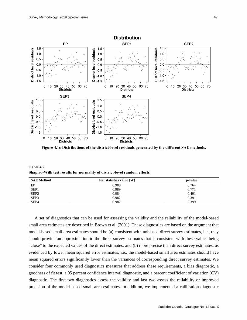
Survey Methodology, 2019 (special issue) 47
Statistics Canada, Catalogue No. 12-001-X
Figure 4.1c Distributions of the district-level residuals generated by the different SAE methods.
Table 4.2 Shapiro-Wilk test results for normality of district-level random effects
SAE Method Test statistics value (W) p-value
EP 0.988 0.764 SEP1 0.989 0.771 SEP2 0.984 0.491 SEP3 0.982 0.391 SEP4 0.982 0.399
A set of diagnostics that can be used for assessing the validity and the reliability of the model-based
small area estimates are described in Brown et al. (2001). These diagnostics are based on the argument that
model-based small area estimates should be (a) consistent with unbiased direct survey estimates, i.e., they
should provide an approximation to the direct survey estimates that is consistent with these values being
“close” to the expected values of the direct estimates; and (b) more precise than direct survey estimates, as
evidenced by lower mean squared error estimates, i.e., the model-based small area estimates should have
mean squared errors significantly lower than the variances of corresponding direct survey estimates. We
consider four commonly used diagnostics measures that address these requirements, a bias diagnostic, a
goodness of fit test, a 95 percent confidence interval diagnostic, and a percent coefficient of variation (CV)
diagnostic. The first two diagnostics assess the validity and last two assess the reliability or improved
precision of the model based small area estimates. In addition, we implemented a calibration diagnostic

48 Chandra, Chambers and Salvati: Small area estimation of survey weighted counts under aggregated level spatial model
Statistics Canada, Catalogue No. 12-001-X
where the model-based estimates are aggregated to higher level and compared with direct survey estimates
at this level. See for example, Chandra et al. (2011). Note that here direct estimates are defined as the survey
weighted direct estimates.
The bias diagnostic is based on following idea. The direct survey estimates are unbiased estimates of the
population values of interest (i.e., true values). If the model-based estimates are “close” to the small area
values of interest, then unbiased direct survey estimators should behave like random variables whose
expected values correspond to the values of the model-based estimates. A Goodness of Fit (GoF) diagnostic,
which is equivalent to a Wald test, for whether the differences between direct and model-based estimates
have a zero mean, can therefore be applied (Brown et al., 2001). This Wald test statistic is computed as
2DIR Model based estimate
DIR Model based estimate
-W .
mse -i i
ii iv
The value of W is compared against the 95th percentile of a chi square distribution with D degrees of
freedom. Here 71D and this 95th percentile value is 91.670. The results from GoF diagnostic are set out
in Table 4.3. We also calculated the average bias (Bias) and average relative difference (RE) between the
direct and the model-based estimates, where
1 Model based estimate DIRBias - i iiD
and
1Model based estimate DIR
DIR
-RE .i i
ii
D
Table 4.4 shows the values of Bias and RE for different SAE methods. The results set out in Tables 4.3
and 4.4 clearly show that the model-based estimates generated by the different SAE methods are consistent
with the direct survey estimates. Finally, in Figure 4.2 we provide a set of bias diagnostic plots, defined by
plotting direct survey estimates (Y -axis) against corresponding model-based estimates ( X -axis) and
testing for divergence of the regression line from the Y X line. These plots show that the model-based
estimates are less extreme when compared to the direct survey estimates, demonstrating the typical SAE
outcome of shrinking more extreme values towards the average. The values of R2 for the fitted (OLS)
regression line between the direct survey estimates and the EP, SEP1, SEP2, SEP3 and SEP4 estimates are
97, 93, 94, 92 and 96 per cent respectively. In general, these different bias diagnostics all show that the
estimates generated by all the SAE methods appear to be consistent with the direct survey estimates.
Table 4.3 Goodness of Fit Diagnostic
SAE Method Goodness of Fit*
EP 23.645 SEP1 30.727 SEP2 27.784 SEP3 30.930 SEP4 24.442 *A small value (< 91.670 in this case) indicates no statistically significant difference between model-based and direct estimates.

Survey Methodology, 2019 (special issue) 49
Statistics Canada, Catalogue No. 12-001-X
Table 4.4 Bias diagnostics between for direct survey (weighted) versus model based estimates
SAE Method Bias RE
EP 0.0023 0.2068 SEP1 0.0007 0.2155 SEP2 0.0016 0.1935 SEP3 0.0013 0.2096 SEP4 0.0016 0.2028
Figure 4.2 Bias diagnostic plots with y = x line (dotted) and regression line (solid) for proportion of poor rural
households in Uttar Pradesh: model-based estimates versus direct survey (weighted) estimates.
0.70
0.65
0.60
0.55
0.50
0.45
0.40
0.35
0.30
0.25
0.20
0.15
0.10
0.05
0.00
Direct survey estim
ate
0.0 0.05 0.10 0.15 0.20 0.25 0.30 0.35 0.40 0.45 0.50 0.55 0.60 0.65 0.70
EP estimate
0.70
0.65
0.60
0.55
0.50
0.45
0.40
0.35
0.30
0.25
0.20
0.15
0.10
0.05
0.00
Direct survey estim
ate
0.0 0.05 0.10 0.15 0.20 0.25 0.30 0.35 0.40 0.45 0.50 0.55 0.60 0.65 0.70
SEP1 estimate
0.70
0.65
0.60
0.55
0.50
0.45
0.40
0.35
0.30
0.25
0.20
0.15
0.10
0.05
0.00
Direct survey estim
ate
0.0 0.05 0.10 0.15 0.20 0.25 0.30 0.35 0.40 0.45 0.50 0.55 0.60 0.65 0.70
SEP2 estimate
0.70
0.65
0.60
0.55
0.50
0.45
0.40
0.35
0.30
0.25
0.20
0.15
0.10
0.05
0.00
Direct survey estim
ate
0.0 0.05 0.10 0.15 0.20 0.25 0.30 0.35 0.40 0.45 0.50 0.55 0.60 0.65 0.70
SEP3 estimate
0.70
0.65
0.60
0.55
0.50
0.45
0.40
0.35
0.30
0.25
0.20
0.15
0.10
0.05
0.00
Direct survey estim
ate
0.0 0.05 0.10 0.15 0.20 0.25 0.30 0.35 0.40 0.45 0.50 0.55 0.60 0.65 0.70
SEP4 estimate

50 Chandra, Chambers and Salvati: Small area estimation of survey weighted counts under aggregated level spatial model
Statistics Canada, Catalogue No. 12-001-X
A second set of diagnostics assess the reliability and improved precision of the model-based estimates
relative to the direct survey estimates. The percent coefficient of variation (CV) is the estimated sampling
standard error as a percentage of the estimate. Small area estimates with large CVs are considered unreliable.
There is no international standard for what constitutes “too large” in this context (Chandra et al., 2011 and
Johnson et al., 2010), but in general, CVs below 10 per cent are preferable for district level estimates.
Table 4.5 provides a summary of CVs of the direct survey estimates and the model-based estimates
generated by the different SAE methods. The results set out in Table 4.5 lead to two conclusions. First, the
CVs of the direct estimates are larger than the CVs of the model-based estimates. Furthermore, the relative
performances of the model-based methods as compared to the direct survey estimates improve with
decreasing district specific observed (or effective) sample sizes. That is, the estimates computed from the
different model-based approaches are more reliable and provide a better indication of rural poverty
incidence in Uttar Pradesh. Second, among five model-based SAE methods considered in this analysis, the
CVs of the spatial EP (3.11), based on the spatial model (3.6) with proximity matrix defined by the four
different spatial proximity functions corresponding to SEP1, SEP2, SEP3 and SEP4 are all smaller than the
CV of the EP (3.4) under the non-spatial model (3.1). That is, the use of spatial information improves the
efficiency of the SAE method. In particular, SEP3 appears to be the best performing method of the four
spatial methods that were investigated. In what follows we therefore focus on the SEP3 predictor only.
Table 4.5 Distributions of CVs for different methods
Value DIR EP SEP1 SEP2 SEP3 SEP4
Minimum 12.92 13.02 12.82 12.73 12.62 12.73 Q1 22.16 20.26 19.02 19.91 19.02 19.59 Median 30.81 24.42 23.76 24.20 22.92 23.78 Mean 35.68 25.35 24.11 24.94 23.95 24.80 Q3 47.64 30.52 27.78 29.12 27.97 29.36 Maximum 99.06 43.21 39.49 42.97 38.56 42.00
Figure 4.3 shows the district-wise distribution of the CVs of the DIR, EP and SEP3 methods. These show
that direct survey estimates of poverty incidence are unstable with CVs that vary from 12.92 to 99.06% with
average of 35.68%. Furthermore, the CVs of the direct survey estimates are greater than 40% and 50% in 7
and 14 (out of 71) districts respectively (see Figure 4.3). In contrast, the average CV values of EP and SEP3
are 25.35% and 23.95% respectively, and the CV of SEP3 is smaller than that of EP in 69 out of 71 districts.
The district-wise plot of the 95 percent confidence intervals (CIs) generated by DIR and SEP3 are
displayed in Figure 4.4. This shows that the 95% CIs for the direct estimates are wider than the 95% CIs for
the model based estimates generated by SEP3. We supplement this visual exploration of 95% CIs by
computing the values of the coverage diagnostic described in Brown et al. (2001) as a way of evaluating the
validity of the confidence intervals generated by the model-based estimates. Here we first calculate adjusted
95% confidence intervals for the direct and model-based estimates using the district-wise critical values
DIR model-based estimate DIR model-based estimate1.96 mse mse .i i i i ic v v
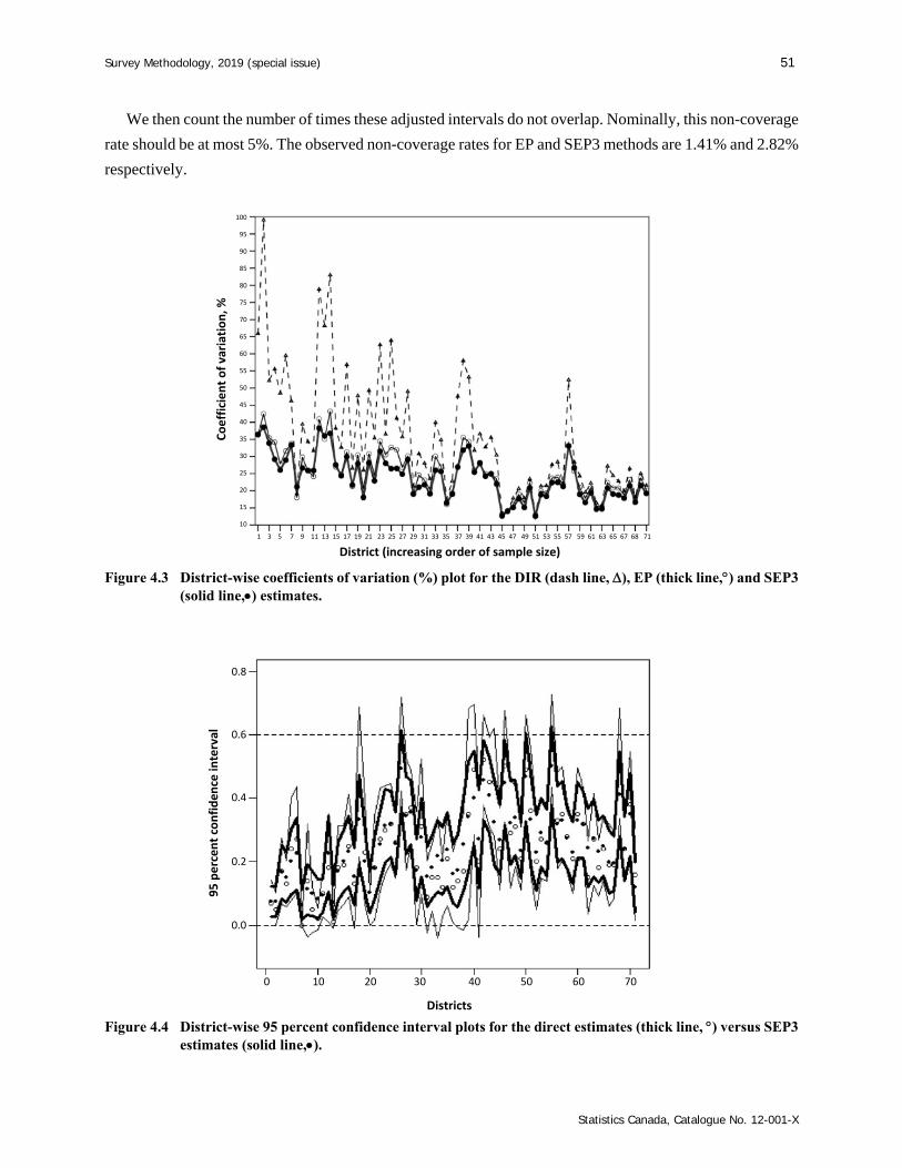
Survey Methodology, 2019 (special issue) 51
Statistics Canada, Catalogue No. 12-001-X
We then count the number of times these adjusted intervals do not overlap. Nominally, this non-coverage
rate should be at most 5%. The observed non-coverage rates for EP and SEP3 methods are 1.41% and 2.82%
respectively.
Figure 4.3 District-wise coefficients of variation (%) plot for the DIR (dash line, ), EP (thick line,) and SEP3 (solid line,) estimates.
Figure 4.4 District-wise 95 percent confidence interval plots for the direct estimates (thick line, ) versus SEP3 estimates (solid line,).
100
95
90
85
80
75
70
65
60
55
50
45
40
35
30
25
20
15
10
Coefficient of variation, %
1 3 5 7 9 11 13 15 17 19 21 23 25 27 29 31 33 35 37 39 41 43 45 47 49 51 53 55 57 59 61 63 65 67 68 71
District (increasing order of sample size)
0.8
0.6
0.4
0.2
0.0
95 percen
t confiden
ce interval
0 10 20 30 40 50 60 70
Districts
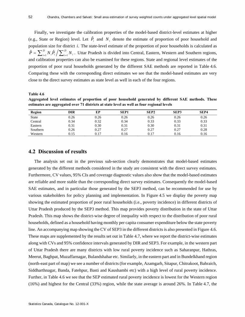
52 Chandra, Chambers and Salvati: Small area estimation of survey weighted counts under aggregated level spatial model
Statistics Canada, Catalogue No. 12-001-X
Finally, we investigate the calibration properties of the model-based district-level estimates at higher
(e.g., State or Region) level. Let ˆiP and iN denote the estimate of proportion of poor household and
population size for district .i The state-level estimate of the proportion of poor households is calculated as
1 1ˆ ˆ .
D D
i i ii iP N P N
Uttar Pradesh is divided into Central, Eastern, Western and Southern regions,
and calibration properties can also be examined for these regions. State and regional level estimates of the
proportion of poor rural households generated by the different SAE methods are reported in Table 4.6.
Comparing these with the corresponding direct estimates we see that the model-based estimates are very
close to the direct survey estimates as state level as well in each of the four regions.
Table 4.6 Aggregated level estimates of proportion of poor household generated by different SAE methods. These estimates are aggregated over 71 districts at state level as well as four regional levels
Region DIR EP SEP1 SEP2 SEP3 SEP4
State 0.26 0.26 0.26 0.26 0.26 0.26 Central 0.34 0.32 0.34 0.33 0.33 0.33 Eastern 0.31 0.30 0.31 0.30 0.31 0.31 Southern 0.26 0.27 0.27 0.27 0.27 0.28 Western 0.15 0.17 0.16 0.17 0.16 0.16
4.2 Discussion of results
The analysis set out in the previous sub-section clearly demonstrates that model-based estimates
generated by the different methods considered in the study are consistent with the direct survey estimates.
Furthermore, CV values, 95% CIs and coverage diagnostic values also show that the model-based estimates
are reliable and more stable than the corresponding direct survey estimates. Consequently the model-based
SAE estimates, and in particular those generated by the SEP3 method, can be recommended for use by
various stakeholders for policy planning and implementation. In Figure 4.5 we display the poverty map
showing the estimated proportion of poor rural households (i.e., poverty incidence) in different districts of
Uttar Pradesh produced by the SEP3 method. This map provides poverty distribution in the state of Uttar
Pradesh. This map shows the district-wise degree of inequality with respect to the distribution of poor rural
households, defined as a household having monthly per capita consumer expenditure below the state poverty
line. An accompanying map showing the CV of SEP3 in the different districts is also presented in Figure 4.6.
These maps are supplemented by the results set out in Table 4.7, where we report the district-wise estimates
along with CVs and 95% confidence intervals generated by DIR and SEP3. For example, in the western part
of Uttar Pradesh there are many districts with low rural poverty incidence such as Saharanpur, Hathras,
Meerut, Baghpat, Muzaffarnagar, Bulandshahar etc. Similarly, in the eastern part and in Bundelkhand region
(north-east part of map) we see a number of districts (for example, Azamgarh, Sitapur, Chitrakoot, Bahraich,
Siddharthnagar, Banda, Fatehpur, Basti and Kaushambi etc) with a high level of rural poverty incidence.
Further, in Table 4.6 we see that the SEP estimated rural poverty incidence is lowest for the Western region
(16%) and highest for the Central (33%) region, while the state average is around 26%. In Table 4.7, the
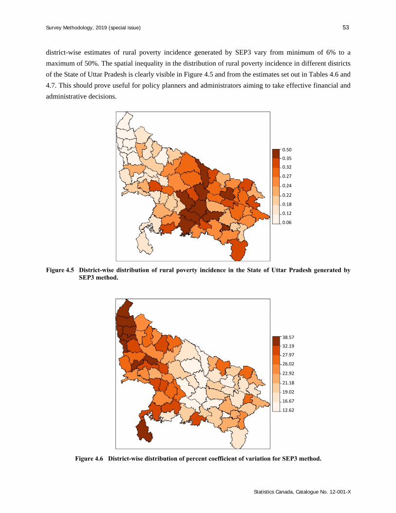
Survey Methodology, 2019 (special issue) 53
Statistics Canada, Catalogue No. 12-001-X
district-wise estimates of rural poverty incidence generated by SEP3 vary from minimum of 6% to a
maximum of 50%. The spatial inequality in the distribution of rural poverty incidence in different districts
of the State of Uttar Pradesh is clearly visible in Figure 4.5 and from the estimates set out in Tables 4.6 and
4.7. This should prove useful for policy planners and administrators aiming to take effective financial and
administrative decisions.
Figure 4.5 District-wise distribution of rural poverty incidence in the State of Uttar Pradesh generated by SEP3 method.
Figure 4.6 District-wise distribution of percent coefficient of variation for SEP3 method.
0.50
0.35
0.32
0.27
0.24
0.22
0.18
0.12
0.06
38.57
32.19
27.97
26.02
22.92
21.18
19.02
16.67
12.62

54 Chandra, Chambers and Salvati: Small area estimation of survey weighted counts under aggregated level spatial model
Statistics Canada, Catalogue No. 12-001-X
Table 4.7 District-wise direct estimates (DIR) and model-based estimates (SEP3) along with their CVs (expressed in percentage terms) and corresponding 95 percent confidence intervals for poverty incidence in the state of Uttar Pradesh in 2011-12
Region District Estimated poverty incidence 95 percent confidence intervals Coefficient of variation, %
DIR SEP3 DIR SEP3 DIR SEP3
Lower Upper Lower Upper
Western Saharanpur 0.07 0.07 0.00 0.14 0.03 0.12 53.16 33.10 Muzaffarnagar 0.05 0.07 0.00 0.10 0.03 0.12 52.36 33.10 Bijnor 0.17 0.17 0.06 0.28 0.08 0.25 31.79 25.41 Moradabad 0.13 0.15 0.06 0.20 0.07 0.23 28.41 26.67 Rampur 0.24 0.20 0.08 0.40 0.10 0.30 34.35 25.98 Jyotiba P. Nagar 0.27 0.23 0.10 0.44 0.11 0.34 31.69 25.92 Meerut 0.00 0.06 0.00 0.00 0.02 0.11 78.83 38.27 Baghpat 0.14 0.11 -0.04 0.32 0.03 0.19 65.87 36.49 Ghaziabad 0.05 0.10 -0.02 0.12 0.03 0.17 68.16 36.06 G. B. Nagar 0.02 0.08 -0.02 0.06 0.02 0.14 99.06 38.56 Bulandshahr 0.10 0.09 0.03 0.17 0.04 0.15 36.60 28.15 Aligarh 0.18 0.23 0.01 0.35 0.11 0.35 47.56 26.91 Mahamaya Nr 0.01 0.07 -0.01 0.03 0.02 0.12 82.97 36.75 Mathura 0.18 0.17 0.05 0.31 0.08 0.26 38.23 27.59 Agra 0.19 0.20 0.07 0.31 0.11 0.30 32.75 24.25 Firozabad 0.25 0.23 0.09 0.41 0.12 0.34 32.69 24.38 Etah 0.13 0.15 -0.01 0.27 0.06 0.24 56.82 29.95 Mainpuri 0.45 0.33 0.22 0.68 0.19 0.47 26.57 21.72 Budaun 0.23 0.20 0.07 0.39 0.10 0.30 35.57 25.00 Bareilly 0.05 0.10 -0.01 0.11 0.04 0.17 57.98 31.89 Pilibhit 0.18 0.18 0.01 0.35 0.08 0.28 47.72 27.93 Shahjahanpur 0.27 0.25 0.11 0.43 0.14 0.36 30.39 22.01 Farrukhabad 0.18 0.17 0.01 0.35 0.08 0.27 49.26 28.16 Kannauj 0.31 0.28 0.10 0.52 0.15 0.40 35.37 22.92 Etawah 0.09 0.15 -0.02 0.20 0.06 0.25 62.63 31.55 Auraiya 0.15 0.18 0.04 0.26 0.08 0.28 36.53 28.02 Kansiram Nr 0.16 0.12 0.02 0.30 0.04 0.20 46.20 33.33
Central Kheri 0.30 0.31 0.16 0.44 0.20 0.43 24.31 18.96 Sitapur 0.32 0.32 0.20 0.44 0.22 0.42 19.56 16.59 Hardoi 0.26 0.26 0.15 0.37 0.16 0.36 22.25 19.46 Unnao 0.57 0.49 0.42 0.72 0.37 0.61 13.36 12.69 Lucknow 0.35 0.35 0.17 0.53 0.22 0.47 26.02 18.10 Rae Bareli 0.37 0.36 0.25 0.49 0.25 0.46 16.46 14.64 Kanpur Dehat 0.15 0.22 -0.04 0.34 0.10 0.33 63.88 26.47 Kanpur Nagar 0.12 0.20 0.02 0.22 0.10 0.31 41.19 26.53 Fatehpur 0.52 0.46 0.38 0.66 0.33 0.58 13.88 14.04
Southern Jalaun 0.21 0.24 0.06 0.36 0.12 0.35 35.70 24.86
Jhansi 0.12 0.16 0.00 0.24 0.07 0.25 48.97 29.13
Lalitpur 0.14 0.17 0.00 0.28 0.06 0.29 52.16 33.90
Hamirpur 0.17 0.25 -0.02 0.36 0.11 0.40 55.55 29.20
Banda 0.49 0.40 0.28 0.70 0.25 0.55 21.36 19.04
Chitrakoot 0.20 0.27 -0.03 0.43 0.12 0.43 59.47 28.95
Mahoba 0.35 0.33 0.20 0.50 0.21 0.45 21.38 18.87
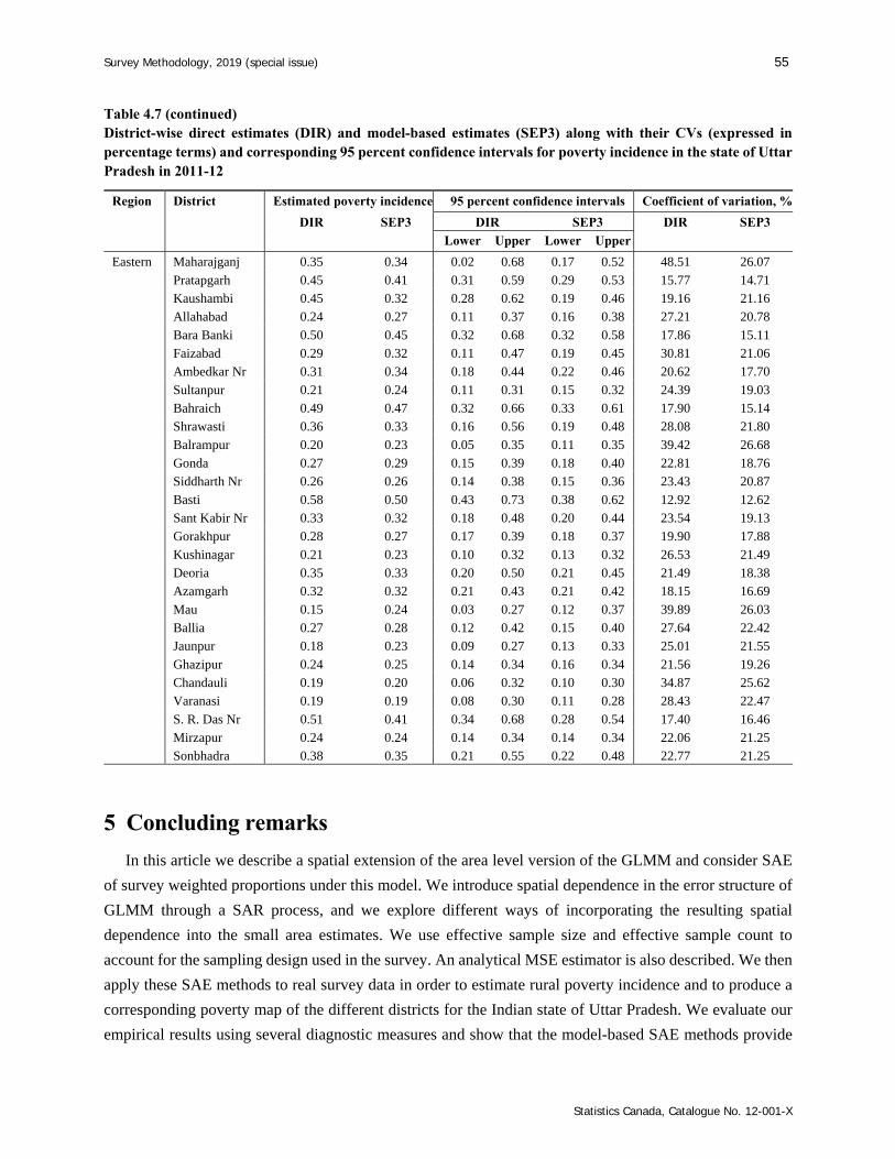
Survey Methodology, 2019 (special issue) 55
Statistics Canada, Catalogue No. 12-001-X
Table 4.7 (continued) District-wise direct estimates (DIR) and model-based estimates (SEP3) along with their CVs (expressed in percentage terms) and corresponding 95 percent confidence intervals for poverty incidence in the state of Uttar Pradesh in 2011-12
Region District Estimated poverty incidence 95 percent confidence intervals Coefficient of variation, %
DIR SEP3 DIR SEP3 DIR SEP3
Lower Upper Lower Upper
Eastern Maharajganj 0.35 0.34 0.02 0.68 0.17 0.52 48.51 26.07
Pratapgarh 0.45 0.41 0.31 0.59 0.29 0.53 15.77 14.71
Kaushambi 0.45 0.32 0.28 0.62 0.19 0.46 19.16 21.16
Allahabad 0.24 0.27 0.11 0.37 0.16 0.38 27.21 20.78
Bara Banki 0.50 0.45 0.32 0.68 0.32 0.58 17.86 15.11
Faizabad 0.29 0.32 0.11 0.47 0.19 0.45 30.81 21.06
Ambedkar Nr 0.31 0.34 0.18 0.44 0.22 0.46 20.62 17.70
Sultanpur 0.21 0.24 0.11 0.31 0.15 0.32 24.39 19.03
Bahraich 0.49 0.47 0.32 0.66 0.33 0.61 17.90 15.14
Shrawasti 0.36 0.33 0.16 0.56 0.19 0.48 28.08 21.80
Balrampur 0.20 0.23 0.05 0.35 0.11 0.35 39.42 26.68
Gonda 0.27 0.29 0.15 0.39 0.18 0.40 22.81 18.76
Siddharth Nr 0.26 0.26 0.14 0.38 0.15 0.36 23.43 20.87
Basti 0.58 0.50 0.43 0.73 0.38 0.62 12.92 12.62
Sant Kabir Nr 0.33 0.32 0.18 0.48 0.20 0.44 23.54 19.13
Gorakhpur 0.28 0.27 0.17 0.39 0.18 0.37 19.90 17.88
Kushinagar 0.21 0.23 0.10 0.32 0.13 0.32 26.53 21.49
Deoria 0.35 0.33 0.20 0.50 0.21 0.45 21.49 18.38
Azamgarh 0.32 0.32 0.21 0.43 0.21 0.42 18.15 16.69
Mau 0.15 0.24 0.03 0.27 0.12 0.37 39.89 26.03
Ballia 0.27 0.28 0.12 0.42 0.15 0.40 27.64 22.42
Jaunpur 0.18 0.23 0.09 0.27 0.13 0.33 25.01 21.55
Ghazipur 0.24 0.25 0.14 0.34 0.16 0.34 21.56 19.26
Chandauli 0.19 0.20 0.06 0.32 0.10 0.30 34.87 25.62
Varanasi 0.19 0.19 0.08 0.30 0.11 0.28 28.43 22.47
S. R. Das Nr 0.51 0.41 0.34 0.68 0.28 0.54 17.40 16.46
Mirzapur 0.24 0.24 0.14 0.34 0.14 0.34 22.06 21.25
Sonbhadra 0.38 0.35 0.21 0.55 0.22 0.48 22.77 21.25
5 Concluding remarks
In this article we describe a spatial extension of the area level version of the GLMM and consider SAE
of survey weighted proportions under this model. We introduce spatial dependence in the error structure of
GLMM through a SAR process, and we explore different ways of incorporating the resulting spatial
dependence into the small area estimates. We use effective sample size and effective sample count to
account for the sampling design used in the survey. An analytical MSE estimator is also described. We then
apply these SAE methods to real survey data in order to estimate rural poverty incidence and to produce a
corresponding poverty map of the different districts for the Indian state of Uttar Pradesh. We evaluate our
empirical results using several diagnostic measures and show that the model-based SAE methods provide

56 Chandra, Chambers and Salvati: Small area estimation of survey weighted counts under aggregated level spatial model
Statistics Canada, Catalogue No. 12-001-X
significant gains in efficiency for generating district level estimates of proportions of poor households.
Furthermore, when spatial correlation between the districts is used appropriately, the model-based estimates
lead to significant gains in terms of efficiency for the district level estimates. For these data, a spatial
proximity measure defined as a Gaussian function of the distances between districts appears to be the most
effective way of incorporating spatial association between the districts. Finally, use of survey information
through effective sample size leads to more representative and realistic estimates.
In the context of estimation of small area counts under unit level small area models, D’Alò, Di Consiglio,
Falorsi, Ranalli and Solari (2012) describe several different ways that spatial information using different
distance measures can be included in analysis. An exploration of these alternative approaches to including
spatial information under area level versions of the corresponding small area models therefore seems
worthwhile. Furthermore, in this article we use a SAR structure to capture the spatial dependence in the
GLMM. However, as noted earlier, there are alternative approaches such as the use of CAR models as well
as newly developed models for spatial nonstationarity that can be used to characterise this spatial
dependence. See, for example, Besag et al. (1991), Leroux et al. (1999), Chandra et al. (2017, 2018). These
approaches should be explored, and we are currently carrying out further research on them.
Finally, we note that the district level estimates of rural poverty incidence produced using the methods
outlined in this paper will be useful for various Departments and Ministries in Government of India as well
as International organizations for their policy research and strategic planning. They will also be useful for
budget allocation and to target welfare interventions by identifying the districts/regions with high rural
poverty incidence. This application also provides evidence that SAE can be used as cost effective and
efficient approach for generating reliable disaggregate level statistics from existing survey data by
combining auxiliary information from different published sources with direct survey estimates.
Acknowledgements
The authors would like to acknowledge the valuable comments and suggestions of the Editor, the
Associate Editor and the two referees. These led to a considerable improvement in the paper. The work of
Hukum Chandra was carried out under an ICAR-National Fellow Project at ICAR-IASRI, New Delhi, India.
The work of Nicola Salvati has been developed under the support of the Progetto di Ricerca di Ateneo From
Survey-based to register-based statistics: a paradigm shift using latent variable models (grant PRA2018-19).
References
Anselin, L. (1992). Spatial Econometrics. Methods and Models. Kluwer Academic, Boston. Banerjee, S., Carlin, B. and Gelfand, A. (2004). Hierarchical Modelling and Analysis for Spatial Data. New
York: Chapman and Hall. Besag, J., York, J. and Mollié, A. (1991). Bayesian image restoration with two applications in spatial
statistics. Annals of the Institute of Statistical Mathematics, 43, 1-59.

Survey Methodology, 2019 (special issue) 57
Statistics Canada, Catalogue No. 12-001-X
Breslow, N.E., and Clayton, D.G. (1993). Approximate inference in generalized linear mixed models. Journal of the American Statistics Association, 88(421), 9-25.
Brown, G., Chambers, R., Heady, P. and Heasman, D. (2001). Evaluation of small area estimation methods - An application to unemployment estimates from the UK LFS. Proceedings: Symposium 2001, Achieving Data Quality in a Statistical Agency: A Methodological Perspective, Statistics Canada.
Chandra, H. (2013). Exploring spatial dependence in area level random effect model for disaggregate level crop yield estimation. Journal of Applied Statistics, 40, 823-842.
Chandra, H., and Salvati, N. (2018). Small area estimation for count data under a spatial dependent aggregated level random effects model. Communications in Statistics - Theory and Methods, 47(5), 1234-1255.
Chandra, H., Chambers, R. and Salvati, N. (2012). Small area estimation of proportions in business surveys. Journal of Statistical Computation and Simulation, 82(6), 783-795.
Chandra, H., Salvati, N. and Chambers, R. (2017). Small area prediction of counts under a non-stationary spatial model. Spatial Statistics, 20, 30-56.
Chandra, H., Salvati, N. and Chambers, R. (2018). Small area estimation under a spatially non-linear model. Computational Statistics and Data Analysis, 126, 19-38.
Chandra, H., Salvati, N. and Sud, U.C. (2011). Disaggregate-level estimates of indebtedness in the state of Uttar Pradesh in India-an application of small area estimation technique. Journal of Applied Statistics, 38(11), 2413-2432.
Cressie, N. (1993). Statistics for Spatial Data. New York: John Wiley & Sons, Inc.
D’Alò, M., Di Consiglio, L., Falorsi, S., Ranalli, M.G. and Solari, F. (2012). Use of spatial information in small area models for unemployment rate estimation at sub-provincial areas in Italy. Journal of the Indian Society of Agricultural Statistics, Special issue on small area estimation, 66(1), 43-54.
Fay, R.E., and Herriot, R. (1979). Estimates of income for small places: An application of James Stein procedures to census data. Journal of the American Statistical Association, 74, 269-277.
Fotheringham, A.S., Brunsdon, C. and Charlton, M.E. (2002). Geographically Weighted Regression. New York: John Wiley & Sons, Inc., West Sussex.
Franco, C., and Bell, W.R. (2013). Applying bivariate binomial/logit normal models to small area estimation. Proceedings of the Joint Statistical Meetings, Section on Survey Research Methods, American Statistical Association, Alexandria, VA, 690-702.
Ghosh, M., Natarajan, K., Stroud, T.W.F. and Carlin, B.P. (1998). Generalized linear model for small-area estimation. Journal of the American Statistical Association, 93, 273-282.
Jiang, J. (2003). Empirical best prediction for small-area inference based on generalized linear mixed models. Journal of Statistical Planning Inference, 111, 117-127.
Johnson, F.A., Chandra, H., Brown, J. and Padmadas, S. (2010). Estimating district-level births attended by skilled attendants in Ghana using demographic health survey and census data: An application of small area estimation technique. Journal of Official Statistics, 26(2), 341-359.

58 Chandra, Chambers and Salvati: Small area estimation of survey weighted counts under aggregated level spatial model
Statistics Canada, Catalogue No. 12-001-X
Korn, E.L., and Graubard, B.I. (1998). Confidence intervals for proportions with small expected number of positive counts estimated from survey data. Survey Methodology, 24, 2, 193-201. Paper available at https://www150.statcan.gc.ca/n1/en/pub/12-001-x/1998002/article/4356-eng.pdf.
Leroux, B., Lei, X. and Breslow, N. (1999). Estimation of disease rates in small areas: A new mixed model for spatial dependence. In Statistical Models in Epidemiology, the Environment and Clinical Trials, (Eds., M. Halloran and D. Berry), 135-178. New York: Springer-Verlag.
Liu, B., Lahiri, P. and Kalton, G. (2014). Hierarchical Bayes modeling of survey-weighted small area proportions. Survey Methodology, 40, 1, 1-13. Paper available at https://www150.statcan.gc.ca/n1/en/pub/12-001-x/2014001/article/14030-eng.pdf.
Lopez-Vizcaino, E., Lombardìa, M. and Morales, D. (2013). Multinomial-based small area estimation of labour force indicators. Statististcal Modelling, 13, 153-178.
Malec, D., Sedransk, J., Moriarity, C.L. and LeClere, F.B. (1997). Small area inference for binary variables in the national health interview survey. Journal of the American Statistical Association, 92, 815-826.
Manteiga, G.W., Lombardia, M.J., Molina, I., Morales, D. and Santamarìa, L. (2007). Estimation of the mean squared error of predictors of small area linear parameters under a logistic mixed model. Computational Statistics and Data Analysis, 51, 2720-2733.
Marhuenda, Y., Molina, I. and Morales, D. (2013). Small area estimation with spatio-temporal Fay-Herriot models. Computational Statistics and Data Analysis, 58, 308-325.
McGilchrist, C.E. (1994). Estimation in generalized mixed models. Journal of the Royal Statistical Society B, 56, 61-69.
Mercer, L., Wakefield, J., Chen, C. and Lumley, T. (2014). A comparison of spatial smoothing methods for small area estimation with sampling weights. Spatial Statistics, 8, 69-85.
Molina, I., Saei, A. and José Lombardìa, M. (2007). Small area estimates of labour force participation under a multinomial logit mixed model. J. R. Statist. Soc. A, 170, 975-1000.
Molina, I., Salvati, N. and Pratesi, M. (2009). Bootstrap for estimating the MSE of the spatial EBLUP. Computational Statistics, 24, 441-458.
Pfeffermann, D. (2002). Small area estimation: New developments and directions. International Statistical Review, 70, 125-143.
Porter, A.T., Wikle, C.K. and Holan, S.H. (2015). Small area estimation via multivariate Fay-Herriot models with latent spatial dependence. Australian and New Zealand Journal of Statistics, 57, 15-29.
Pratesi, M., and Salvati, N. (2008). Small area estimation - the EBLUP estimator based on spatially correlated random area effects. Statistical Methods and Applications, 17, 114-131.
Pratesi, M., and Salvati, N. (2009). Small area estimation in the presence of correlated random area effects. Journal of Official Statistics, 25, 37-53.
Rao, J.N.K. (2003). Small Area Estimation. New York: John Wiley & Sons, Inc.
Rao, J.N.K., and Molina, I. (2015). Small Area Estimation, 2nd Edition. New York: John Wiley & Sons, Inc.
Survey Methodology, 2019 (special issue) 59
Statistics Canada, Catalogue No. 12-001-X
Saei, A., and Chambers, R. (2003). Small area estimation under linear and generalized linear mixed models with time and area effects. Southampton Statistical Sciences Research Institute, S3RI Methodology Working Papers, M03/15.
Salvati, N., Chandra, H. and Chambers, R. (2012). Model based direct estimation of small area distributions.
Australian & New Zealand Journal of Statistics, 54(1), 103-123. Särndal, C.-E., Swensson, B. and Wretman, J.H. (1992). Model Assisted Survey Sampling. New York:
Springer-Verlag. Singh, B.B., Shukla, G.K. and Kundu, D. (2005). Spatio-temporal models in small area estimation. Survey
Methodology, 31, 2, 183-195. Paper available at https://www150.statcan.gc.ca/n1/en/pub/12-001-x/2005002/article/9053-eng.pdf.
Tzavidis, N., Salvati, N., Pratesi, M. and Chambers, R. (2008). M-quantile models with application to
poverty mapping. Statistical Methods & Applications, 17(3), 393-411.

Survey Methodology, 2019 (special issue) 61 Vol. 45, No. 1, pp. 61-80 Statistics Canada, Catalogue No. 12-001-X
1. William R. Bell, U.S. Census Bureau, Washington, DC 20233, U.S.A. E-mail: [email protected]; Hee Cheol Chung, University of
Georgia, Athens, GA 30602, U.S.A.; Gauri S. Datta, U.S. Census Bureau, Washington, DC 20233, U.S.A. and University of Georgia, Athens, GA 30602, U.S.A.; Carolina Franco, U.S. Census Bureau, Washington, DC 20233, U.S.A.
Measurement error in small area estimation: Functional versus structural versus naïve models
William R. Bell, Hee Cheol Chung, Gauri S. Datta and Carolina Franco1
Abstract
Small area estimation using area-level models can sometimes benefit from covariates that are observed subject to random errors, such as covariates that are themselves estimates drawn from another survey. Given estimates of the variances of these measurement (sampling) errors for each small area, one can account for the uncertainty in such covariates using measurement error models (e.g., Ybarra and Lohr, 2008). Two types of area-level measurement error models have been examined in the small area estimation literature. The functional measurement error model assumes that the underlying true values of the covariates with measurement error are fixed but unknown quantities. The structural measurement error model assumes that these true values follow a model, leading to a multivariate model for the covariates observed with error and the original dependent variable. We compare and contrast these two models with the alternative of simply ignoring measurement error when it is present (naïve model), exploring the consequences for prediction mean squared errors of use of an incorrect model under different underlying assumptions about the true model. Comparisons done using analytic formulas for the mean squared errors assuming model parameters are known yield some surprising results. We also illustrate results with a model fitted to data from the U.S. Census Bureau’s Small Area Income and Poverty Estimates (SAIPE) Program.
Key Words: Sample survey; Area level model; Covariate; Prediction.
1 Introduction
Linear mixed models, particularly that of Fay and Herriot (1979), have gotten great attention in small
area estimation. The Fay-Herriot (FH) model can be written
= = = 1, ,i i i i i iY e z u i m (1.1)
where, for areas i indexed from 1 to ,m the iY are direct survey estimates of population quantities ,i the
sampling errors ie in iY are assumed independent 0, iN D with the iD taken as known (they are actually
estimated using survey micro-data), the iz are 1q vectors of regression covariates with corresponding
coefficient vector , and the random effects iu are distributed 2i.i.d. 0, uN and independently of
the .ie
In some cases it may be desired to augment the model for i with one or more covariates iX that are
themselves estimates taken from another survey that estimates characteristics believed to be related to .i
One approach is to simply ignore the sampling error in ,iX treating it like the covariates in iz which we
shall assume are not subject to sampling or other measurement errors. We shall call this the naïve Fay-
Herriot model, which, taking for simplicity the case of a single such covariate ,iX we write as
,= = .i i i i N i i N i NY e X z u (1.2)
62 Bell et al.: Measurement error in small area estimation: Functional versus structural versus naïve models
Statistics Canada, Catalogue No. 12-001-X
We add the “ ”N subscripts to the regression coefficients and the random effects ,i Nu to distinguish this
model from the measurement error models to come. The model assumes that , i.i.d.i Nu 2,0, ,u NN
although with heteroscedastic sampling error in iX the assumption that ,var i Nu is constant is incorrect,
implying that the model (1.2) is misspecified. This point is discussed further below.
An alternative to the naïve FH model is to use a measurement error model to account for the sampling
(measurement) error in .iX Assume ix denotes the population characteristic being estimated by iX with
sampling error ,i where the i are assumed distributed independently 0, iN C and with the iC taken
as known (actually estimated using survey micro-data). A generalization of the model (1.1) to include the
covariate iX while accounting for its sampling error is
= =i i i i i i iY e x z u (1.3)
= .i i iX x (1.4)
If the ix are assumed to be fixed unknown quantities, then the model defined by (1.3)-(1.4) is known as the
functional measurement error model (FME model). This model is discussed by Fuller (1987) and has been
studied for small area estimation by Ybarra and Lohr (2008), Arima, Datta and Liseo (2015, 2016), and
Arima, Bell, Datta, Franco and Liseo (2017). Analogous unit level measurement error models for small area
estimation have been studied by Ghosh and Sinha (2007), Datta, Rao and Torabi (2010), and Arima, Datta,
and Liseo (2012).
Another alternative to the naïve FH model is to specify a model for ix in (1.4) which, with (1.3), implies
bivariate models for ,i ix and , .i iY X This is known as a structural measurement error model (SME
model). If ix follows the regression model = ,i xi x ix z v with covariates xiz and residuals i.i.d.iv
20, vN independent of ,iu then the resulting model for ,i iY X can be written as
0
= i.i.d. 0, =0
i i i i i
i i i i i
Y e e DN
X x C
(1.5)
=0
i i ii xi
x i ixi
u v ez z
vz
(1.6)
2 2 2 2
2 2
i.i.d. 0, = .i i u v v
i v v
u vN
v
(1.7)
This model differs from a standard bivariate FH model in that the parameter affects both the regression
mean function for iY and the random effect covariance matrix . However, if the covariates xiz are linear
functions of the covariates ,iz then the fixed effects regression part of (1.6) can be reparameterized to
unrestricted linear regression effects i y xi xz z with regression covariates iz for the first equation and
xiz for the second. With this reparameterization no longer affects the regression fixed effects, so the
matrix can then be reparameterized in the general form = ,jk or by 11 , 22 , and
Survey Methodology, 2019 (special issue) 63
Statistics Canada, Catalogue No. 12-001-X
12 11 22= 1, 1 , as there is now a 1-1 correspondence between 2 2, ,u v and
11 22 12, , or 11 22, , . Two instances where this condition on xiz holds are (i) if the regression
covariates are the same in both equations = ,xi iz z or (ii) if xiz is just an intercept term = 1xiz and iz
also includes an intercept.
Datta, Delaigle, Hall and Wang (2018) study the area level SME model, while Huang and Bell (2012)
present a study examining use of general bivariate models for small area estimation. Analogous unit level
models have been studied by Ghosh, Sinha and Kim (2006) and Torabi, Datta and Rao (2009). Fuller (1987)
and Buonaccorsi (2010) discuss additional measurement error models including nonlinear models and the
Berkson model.
Note that the FME and SME models model the relation between the true unobserved quantities i and
,ix whereas the naïve FH model models the relation between i and the observed .iX The iX contain
noise in the form of generally heteroscedastic sampling error, and this heteroscedasticity produces the naïve
model’s misspecification noted earlier.
If iY and iX are estimates from the same survey sample their sampling errors ie and i are likely to
be correlated. This can be accommodated by replacing the off-diagonal 0 of in (1.5) by the appropriate
cov ,i ie (estimated using survey micro-data). While this works for the SME model, correlation between
ie and i implies that the regressor iX and sampling error ie are correlated, violating a fundamental
assumption of the FH model and causing potentially severe problems for the naïve FH model. Hence, we
do not consider that situation here.
In this paper we compare the three alternative models – naïve FH, functional measurement error, and
structural measurement error – focusing on their predictive performance for small area estimation. One
motivating case involves the use of the naïve FH model when measurement error i is present, comparing
the naïve FH model’s predictive accuracy with those of the other two models. We also compare the
predictive performance of the functional versus structural measurement error models. We make these
comparisons using analytic formulas for the mean squared errors (MSEs) for the case where model
parameters are known (first order approximations). This provides good approximations for the case when
the number of areas m is large. It is also relevant as the typically dominant term in the MSEs for smaller
values of .m Since the naïve FH model is misspecified, we make precise in what sense its parameters are
“known”.
Section 2 summarizes some theoretical results for the three alternative models, first on convergence of
parameter estimates and then on small area prediction, covering both the point predictors and their MSEs.
We provide results for the three models first for the case where the FME model is true, and then for the case
where the SME model is true. Derivations of these results are deferred to a corresponding technical report
(Bell, Chung, Datta, and Franco, 2018). Section 3 compares, via contour plots, the theoretical MSEs of small
area predictors for the three models across ranges of the parameters of a true SME model. Section 4 uses
the theoretical MSE formulas to compare prediction MSEs from the three models when they are applied to

64 Bell et al.: Measurement error in small area estimation: Functional versus structural versus naïve models
Statistics Canada, Catalogue No. 12-001-X
an empirical example of modeling poverty rates of school-age children for U.S. counties. The example is
taken from the U.S. Census Bureau’s Small Area Income and Poverty Estimates (SAIPE) program.
Section 5 then gives general conclusions.
2 Theoretical results
To facilitate interpretation of the results, here we use the simplest possible versions of the models
outlined in the Introduction, specifically, models where the vector of non-measurement error covariates
reduces to just an intercept term, i.e., = 1.iz To revert to fairly standard notation, we use for the intercept
coefficient instead of , so the simplified model for i in the FME and SME models (from (1.3)) becomes
= .i i ix u (2.1)
For the SME model we assume that i.i.d.ix 2, xN so there are no regression terms other than the
mean in the model for .ix
For the naïve FH model (1.2), the simplified model for i becomes
,=i N N i i NX u (2.2)
where, as before, we use the N“ ” subscript to distinguish the coefficients and random effects in the naïve
model (2.2) for ,i since this model differs from (2.1) by substituting iX in place of .ix
We now give some results on parameter estimation and small area prediction for these models. The
Appendix of Bell et al. (2018) provides derivations of these results.
2.1 Parameter estimators and their large sample limits
The Appendix of Bell et al. (2018) details unbiased estimating equations for the parameters of the three
models considered here. The resulting estimators of , , and 2u for the simplified versions of the FME
and SME models are the same, and are given by
1=1
21=1
22 2
=1
ˆ =
ˆˆ =
1 ˆ ˆˆˆ =
m
i im im
im i
m
u i ii
X X Y Y
X X C
Y X
Y X D Cm
(2.3)
where 1=1
= ,m
iiX m X with analogous definitions of ,Y ,C and .D For fitting the SME model, we also
have ˆ = X and 212=1
ˆ = .m
x im iX X C Result 1 gives the probability limits of all these parameter
estimators.

Survey Methodology, 2019 (special issue) 65
Statistics Canada, Catalogue No. 12-001-X
Result 1: For the FME and SME models given by (1.3)-(1.4) and by (1.5)-(1.7), respectively, but with the
simplified model for i as in (2.1), the parameter estimators given in (2.3) are consistent for the true model
parameters, that is,
2 2ˆ ˆ ˆP P P
u u (2.4)
where P denotes convergence in probability as m under the true model (whether FME or SME).
For fitting the SME model when it is true, we also have ˆP and 2 2ˆ .
P
x x For fitting the SME
model when the FME model is true, we have 1=1
ˆ = limmP
m im ix x and 2 2ˆ =
P
x xs
21=1
,limm
m im ix x with both limits assumed to exist.
Remark 1: The estimators in (2.3) are the same for the two models despite being obtained from different
estimating equations – see equations (19) and (20) versus equations (36)-(38) in Bell et al. (2018). The
consistency results in (2.4) thus hold whether the true model is the FME or the SME. These consistency
results also hold for the more general versions of these models considered in the Appendix of Bell et al.
(2018).
The parameter estimators for fitting the naïve FH model with the simplified model for i as in (2.2) are
given by
21 1
=1 =12 2
1 1=1 =1
22,
=1
ˆ ˆ= =
ˆˆ =
1 ˆˆˆ = .
m m
i i im mi iN m m
i im mi i
N N
m
u N i N N ii
X X Y Y X X C
X X X X
Y X
Y X Dm
(2.5)
Result 2: When the FME model (or SME model) is true, the parameter estimators in (2.5) have the following
probability limits:
2 2 2,
2 2 2* * , *
ˆ ˆ ˆ1 FME model true
ˆ ˆ ˆ1 SME model true
P P P
N N u N u
P P P
N N u N u
a a x a C
a a a C
where the “attenuation factors” are given by
2 2
*2 2= FME model true = SME model true .x x
x x
sa a
s C C
(2.6)
Remark 2: The results for convergence of ˆN in Result 2 are versions of the well-known attenuation of
the estimate of the regression parameter when measurement error is ignored – see Theil (1971, page 608)
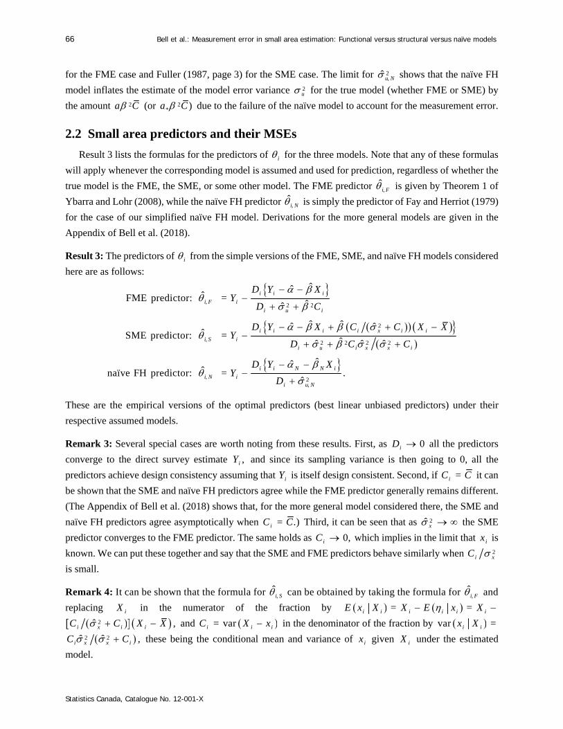
66 Bell et al.: Measurement error in small area estimation: Functional versus structural versus naïve models
Statistics Canada, Catalogue No. 12-001-X
for the FME case and Fuller (1987, page 3) for the SME case. The limit for 2,ˆ u N shows that the naïve FH
model inflates the estimate of the model error variance 2u for the true model (whether FME or SME) by
the amount 2a C (or 2* )a C due to the failure of the naïve model to account for the measurement error.
2.2 Small area predictors and their MSEs
Result 3 lists the formulas for the predictors of i for the three models. Note that any of these formulas
will apply whenever the corresponding model is assumed and used for prediction, regardless of whether the
true model is the FME, the SME, or some other model. The FME predictor ,i F is given by Theorem 1 of
Ybarra and Lohr (2008), while the naïve FH predictor ,i N is simply the predictor of Fay and Herriot (1979)
for the case of our simplified naïve FH model. Derivations for the more general models are given in the
Appendix of Bell et al. (2018).
Result 3: The predictors of i from the simple versions of the FME, SME, and naïve FH models considered
here are as follows:
,2 2
2
,2 2 2 2
, 2,
ˆˆˆFME predictor: =
ˆˆ
ˆ ˆˆ ˆˆSME predictor: =
ˆˆ ˆ ˆ
ˆˆˆnaïve FH predictor: = .
ˆ
i i i
i F i
i u i
i i i i x i i
i S i
i u i x x i
i i N N i
i N ii u N
D Y XY
D C
D Y X C C X XY
D C C
D Y XY
D
These are the empirical versions of the optimal predictors (best linear unbiased predictors) under their
respective assumed models.
Remark 3: Several special cases are worth noting from these results. First, as 0iD all the predictors
converge to the direct survey estimate ,iY and since its sampling variance is then going to 0, all the
predictors achieve design consistency assuming that iY is itself design consistent. Second, if =iC C it can
be shown that the SME and naïve FH predictors agree while the FME predictor generally remains different.
(The Appendix of Bell et al. (2018) shows that, for the more general model considered there, the SME and
naïve FH predictors agree asymptotically when = .)iC C Third, it can be seen that as 2ˆ x the SME
predictor converges to the FME predictor. The same holds as 0,iC which implies in the limit that ix is
known. We can put these together and say that the SME and FME predictors behave similarly when 2i xC
is small.
Remark 4: It can be shown that the formula for ,i S can be obtained by taking the formula for ,i F and
replacing iX in the numerator of the fraction by = =i i i i i iE x X X E x X
2ˆ ,i x i iC C X X and = vari i iC X x in the denominator of the fraction by var =i ix X
2 2ˆ ˆ ,i x x iC C these being the conditional mean and variance of ix given iX under the estimated
model.

Survey Methodology, 2019 (special issue) 67
Statistics Canada, Catalogue No. 12-001-X
Table 2.1 gives, for the case when the FME model is true, the first order biases and prediction error
variances of the three predictors. The MSEs are then the squared biases plus the variances. (The prediction
error variance, and thus the MSE, for the FME model is given by Theorem 1 of Ybarra and Lohr (2008).)
The results assume the true FME model parameters are known, but for the naïve FH model they account for
the fact that the estimates of the parameters are biased as shown in Result 2. This gives a realistic
approximation for the case when ,m the number of areas, is large. The Table 2.1 entries for the SME model
use the quantity
2 2 2 2= .i u i x i x iF D s C s C (2.7)
Table 2.1 Biases and prediction error variances when the FME model is true
Prediction model Bias Prediction error variance
FME 0 2 2
2 2
u i i
u i i
C D
C D
SME i i
ii
D Cx x
F
2 2 2 2 2i x i x i i
ii
D s C s C FD
F
naïve FH
2 2
1ii
u i
D ax x
a C D
22 2
2 2 2 2
u i ii
u i u i
a C D Da aC C
a C D a C D
Table 2.2 gives the results for the case when the SME model is true. In this case all the predictors are
unbiased in the sense that ˆ = 0.i iE Hence, the table just gives the prediction error variances, which
are also the MSEs. For *iF in Table 2.2, we substitute 2
x for 2xs in the expression (2.7), analogous to the
definition of *a in (2.6).
Table 2.2 Prediction error variances when the SME model is true
Prediction model Prediction error variance = MSE
FME 2 2
2 2
u i i
u i i
C D
C D
SME 2 2
*
i x ii
i
D CD
F
naïve FH 22 2
* 2*2 2 2 2
* *
u i ii
u i u i
a C D Da C C
a C D a C D
Several points are worth noting about the results of Tables 2.1 and 2.2.
1. The results for the FME predictor are the same in both cases, i.e., whether the FME or SME
model is true. To achieve unbiasedness under the assumption that the ix are fixed, unknown
quantities, the FME predictor eliminates them from the prediction error. Hence, its prediction
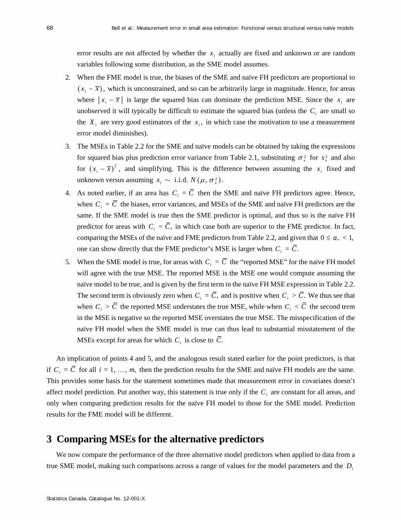
68 Bell et al.: Measurement error in small area estimation: Functional versus structural versus naïve models
Statistics Canada, Catalogue No. 12-001-X
error results are not affected by whether the ix actually are fixed and unknown or are random
variables following some distribution, as the SME model assumes.
2. When the FME model is true, the biases of the SME and naïve FH predictors are proportional to
,ix x which is unconstrained, and so can be arbitrarily large in magnitude. Hence, for areas
where ix x is large the squared bias can dominate the prediction MSE. Since the ix are
unobserved it will typically be difficult to estimate the squared bias (unless the iC are small so
the iX are very good estimators of the ,ix in which case the motivation to use a measurement
error model diminishes).
3. The MSEs in Table 2.2 for the SME and naïve models can be obtained by taking the expressions
for squared bias plus prediction error variance from Table 2.1, substituting 2x for 2
xs and also
for 2 ,ix x and simplifying. This is the difference between assuming the ix fixed and
unknown versus assuming i.i.d.ix 2, .xN
4. As noted earlier, if an area has =iC C then the SME and naïve FH predictors agree. Hence,
when =iC C the biases, error variances, and MSEs of the SME and naïve FH predictors are the
same. If the SME model is true then the SME predictor is optimal, and thus so is the naïve FH
predictor for areas with = ,iC C in which case both are superior to the FME predictor. In fact,
comparing the MSEs of the naïve and FME predictors from Table 2.2, and given that *0 < 1,a
one can show directly that the FME predictor’s MSE is larger when = .iC C
5. When the SME model is true, for areas with =iC C the “reported MSE” for the naïve FH model
will agree with the true MSE. The reported MSE is the MSE one would compute assuming the
naïve model to be true, and is given by the first term in the naïve FH MSE expression in Table 2.2.
The second term is obviously zero when = ,iC C and is positive when > .iC C We thus see that
when >iC C the reported MSE understates the true MSE, while when <iC C the second term
in the MSE is negative so the reported MSE overstates the true MSE. The misspecification of the
naïve FH model when the SME model is true can thus lead to substantial misstatement of the
MSEs except for areas for which iC is close to .C
An implication of points 4 and 5, and the analogous result stated earlier for the point predictors, is that
if =iC C for all = 1, , ,i m then the prediction results for the SME and naïve FH models are the same.
This provides some basis for the statement sometimes made that measurement error in covariates doesn’t
affect model prediction. Put another way, this statement is true only if the iC are constant for all areas, and
only when comparing prediction results for the naïve FH model to those for the SME model. Prediction
results for the FME model will be different.
3 Comparing MSEs for the alternative predictors
We now compare the performance of the three alternative model predictors when applied to data from a
true SME model, making such comparisons across a range of values for the model parameters and the iD

Survey Methodology, 2019 (special issue) 69
Statistics Canada, Catalogue No. 12-001-X
and iC values. The comparisons use the MSE results of Table 2.2, examining percentage differences in the
MSEs calculated, for example, as
MSE
100 1MSE
F
S
(3.1)
for comparing MSEs of the FME and SME predictors. We similarly define the analogs to (3.1) for
comparing MSEs for the naïve FH and FME predictors, and of the naïve FH and SME predictors, as well
as for comparing the reported and actual MSEs of the naïve FH predictor. Assuming that the SME model is
true facilitates the comparisons. Assuming that the FME model is true leads to the complication that the
MSEs for the structural and naïve models depend on ix (Table 2.1), which has unrestricted variation over
areas. Section 4 nonetheless makes some MSE comparisons under a true FME model.
For making relative comparisons as in (3.1) the scale of the data doesn’t matter, so rescaling to i uY
will not affect these comparisons. This is also true for rescaling iX to .i xX These rescalings reduce the
number of varying parameters we need to consider by two, which lets us express 21 u times MSE ,F
MSE ,S MSE ,N and MSE N (the reported MSE for the naïve FH predictor), all computed assuming the
SME model is true, in terms of the following four scale independent quantities:
2 2 2
= , = , = corr , , = .i iD C i i C
u x x
D C Cr r x r
(3.2)
The Appendix illustrates such re-expression for the calculation of 2MSE .S u To simplify the notation, we
omit the i subscript from Dr and ,Cr though except in the unusual situation where the iD and iC are
actually constant over areas, one needs to compute the MSE expressions separately for each area .i To
compare MSEs we examine contour plots over ,D Cr r for each of the MSE percentage differences defined
as in (3.1), viewing the MSE percentage difference as a function of , .D Cr r We examine such plots for
fixed values of and Cr (which do not vary over ).i
Figure 3.1 gives contour plots of (3.1) for = 0.3 and = 0.7. The x- and y-axes of the plots,
representing the values of Dr and ,Cr range from 0.1 to 10, and are shown with log scaling. We need not
set Cr for these comparisons because MSE F and MSE S do not depend on .C The results in the plots are
easy to summarize: the percentage differences are all positive, favoring the SME model which here is
assumed to be true, and the differences increase with both Dr and ,Cr so that the more sampling or
measurement error is present, the larger is the advantage to use of the SME predictor. When either Dr or Cr
is small, say generally below 1, the MSE percentage differences are small, which is why no contours show
up plotted in this area, and choice of model has little effect on prediction accuracy. In fact, when both Dr
and Cr are sufficiently small the FME and SME predictors are both close to the direct estimator ,iY leading
to small MSE differences, a pattern repeated in subsequent graphs. Towards the upper right corner the MSE
percentage differences become substantial in both graphs, larger for = 0.7. Analysis of the formula for
MSE MSEF S reveals that, for given values of Cr and ,Dr the MSE percent differences increase with
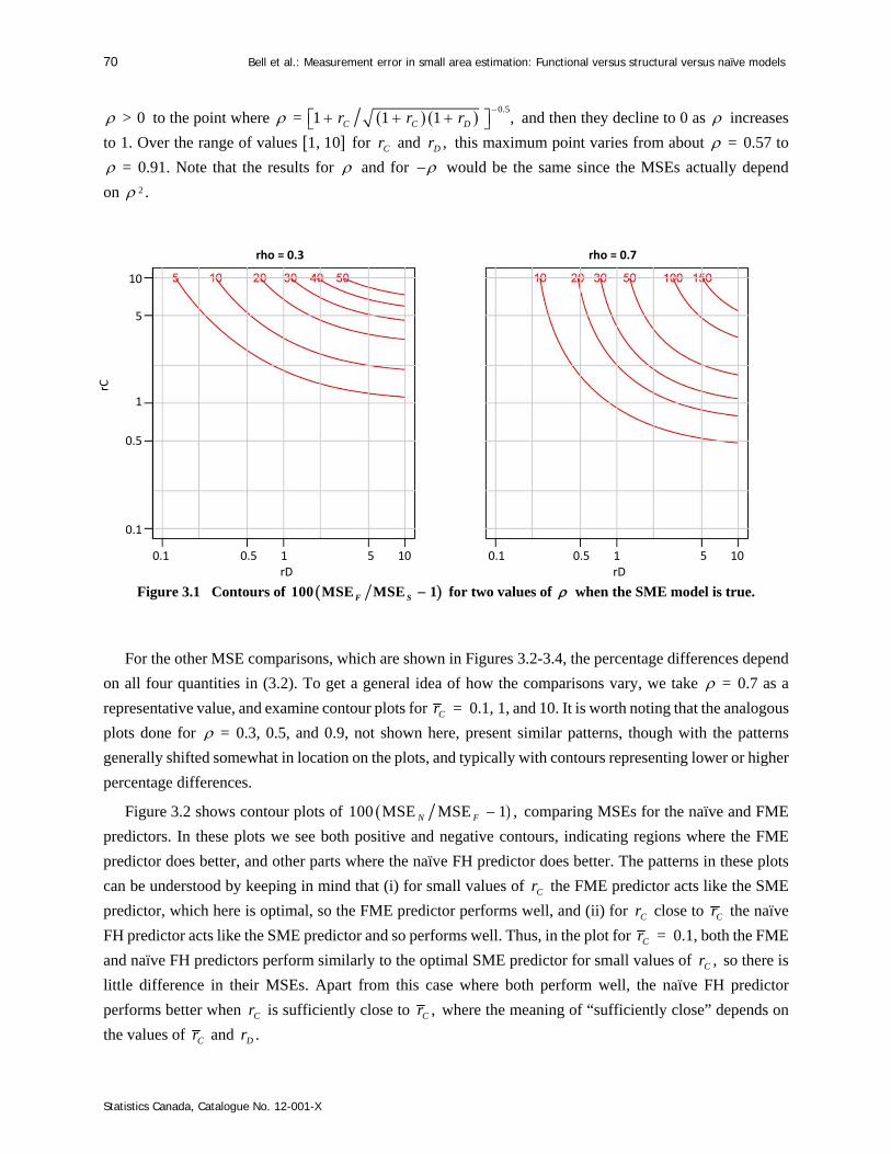
70 Bell et al.: Measurement error in small area estimation: Functional versus structural versus naïve models
Statistics Canada, Catalogue No. 12-001-X
> 0 to the point where 0.5
= 1 1 1 ,C C Dr r r
and then they decline to 0 as increases
to 1. Over the range of values 1, 10 for Cr and ,Dr this maximum point varies from about = 0.57 to
= 0.91. Note that the results for and for would be the same since the MSEs actually depend
on 2 .
Figure 3.1 Contours of 100 MSE MSE 1F S for two values of when the SME model is true.
For the other MSE comparisons, which are shown in Figures 3.2-3.4, the percentage differences depend
on all four quantities in (3.2). To get a general idea of how the comparisons vary, we take = 0.7 as a
representative value, and examine contour plots for =Cr 0.1, 1, and 10. It is worth noting that the analogous
plots done for = 0.3, 0.5, and 0.9, not shown here, present similar patterns, though with the patterns
generally shifted somewhat in location on the plots, and typically with contours representing lower or higher
percentage differences.
Figure 3.2 shows contour plots of 100 MSE MSE 1 ,N F comparing MSEs for the naïve and FME
predictors. In these plots we see both positive and negative contours, indicating regions where the FME
predictor does better, and other parts where the naïve FH predictor does better. The patterns in these plots
can be understood by keeping in mind that (i) for small values of Cr the FME predictor acts like the SME
predictor, which here is optimal, so the FME predictor performs well, and (ii) for Cr close to Cr the naïve
FH predictor acts like the SME predictor and so performs well. Thus, in the plot for =Cr 0.1, both the FME
and naïve FH predictors perform similarly to the optimal SME predictor for small values of ,Cr so there is
little difference in their MSEs. Apart from this case where both perform well, the naïve FH predictor
performs better when Cr is sufficiently close to ,Cr where the meaning of “sufficiently close” depends on
the values of Cr and .Dr
10
5
1
0.5
0.1
0.1 0.5 1 5 10 0.1 0.5 1 5 10 rD rD
rC
rho = 0.3 rho = 0.7

Survey Methodology, 2019 (special issue) 71
Statistics Canada, Catalogue No. 12-001-X
Figure 3.2 Contours of 100 MSE MSE 1N F for = 0.7 and =Cr 0.1, 1, and 10 when the SME model is true.
The results in Figure 3.2 showing that for certain regions the naïve FH predictor has lower prediction
MSE than the FME predictor may at first seem surprising given that, when the SME model is true, the naïve
model is misspecified since it ignores the measurement error in .iX In contrast, the FME model accounts
for the measurement error in iX and, since it makes no assumptions about the ,ix it is not inconsistent with
the true SME model. In fact, as we move towards larger amounts of measurement error overall (larger values
of ),Cr the MSE advantages of the naïve FH predictor become more substantial and cover larger ranges of
the Cr and Dr values. The general explanation for this is that, when measurement error is substantial, the
FME model’s avoidance of any modeling assumptions about the ix can lead to rather inefficient use of the
data ,iX while the naïve FH predictor makes suboptimal but better use of the iX unless Cr is very different
from Cr (equivalently, iC is very different from ).C
Figure 3.3 gives contour plots of 100 MSE MSE 1 ,N S comparing MSEs for the naïve and SME
predictors. Since the SME model is assumed true for the purposes of these computations, all the contours
shown are positive, with the exception of a zero line in each plot (represented here by the contour plotting
function of R (R core team, 2016) as a set of “0” labels not joined by a line). These zero contours occur as
horizontal lines for =Cr 0.1, 1, and 10 on the three plots, these being where = ,C Cr r implying = ,iC C
which is when the naïve FH and SME predictors agree. Apart from this, the plots for =Cr 0.1 and 1 show
substantial positive contours for large values of Cr that also increase with ,Dr while for =Cr 10 the
substantial positive contours occur for small Cr as Dr grows large.
Figure 3.3 Contours of 100 MSE MSE 1N S for = 0.7 and =Cr 0.1, 1, and 10 when the SME model is true.
10
2
1
0.5
0.1
0.1 0.5 1 2 10 0.1 0.5 1 2 10 0.1 0.5 1 2 10 rD rD rD
rC
rho = 0.7, rCbar = 0.1 rho = 0.7, rCbar = 1 rho = 0.7, rCbar = 10 10
2
1
0.5
0.1
10
2
1
0.5
0.1
10
2
1
0.5
0.1
0.1 0.5 1 2 10 0.1 0.5 1 2 10 0.1 0.5 1 2 10 rD rD rD
rC
rho = 0.7, rCbar = 0.1 rho = 0.7, rCbar = 1 rho = 0.7, rCbar = 10 10
2
1
0.5
0.1
10
2
1
0.5
0.1
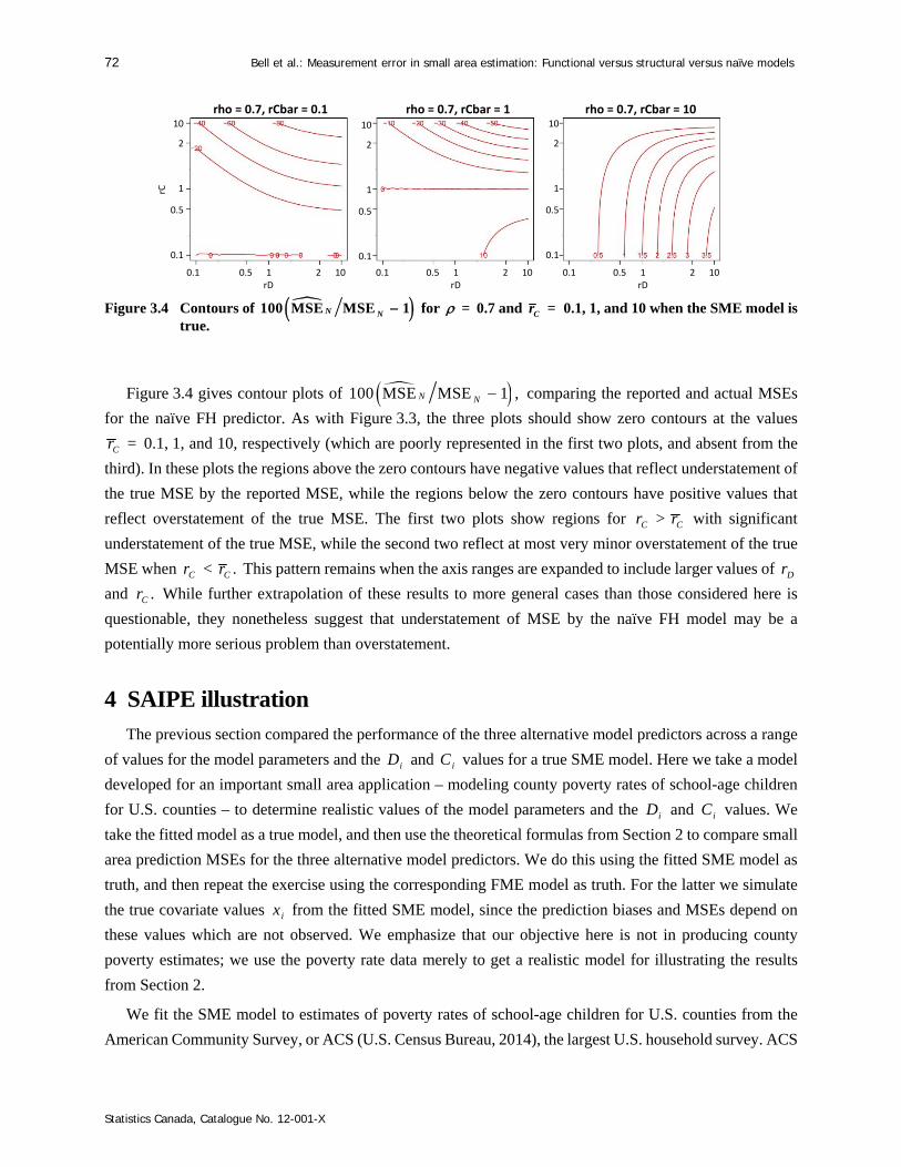
72 Bell et al.: Measurement error in small area estimation: Functional versus structural versus naïve models
Statistics Canada, Catalogue No. 12-001-X
Figure 3.4 Contours of 100 MSE MSE 1N N for = 0.7 and =Cr 0.1, 1, and 10 when the SME model is true.
Figure 3.4 gives contour plots of 100 MSE MSE 1 ,N N comparing the reported and actual MSEs
for the naïve FH predictor. As with Figure 3.3, the three plots should show zero contours at the values
=Cr 0.1, 1, and 10, respectively (which are poorly represented in the first two plots, and absent from the
third). In these plots the regions above the zero contours have negative values that reflect understatement of
the true MSE by the reported MSE, while the regions below the zero contours have positive values that
reflect overstatement of the true MSE. The first two plots show regions for >C Cr r with significant
understatement of the true MSE, while the second two reflect at most very minor overstatement of the true
MSE when < .C Cr r This pattern remains when the axis ranges are expanded to include larger values of Dr
and .Cr While further extrapolation of these results to more general cases than those considered here is
questionable, they nonetheless suggest that understatement of MSE by the naïve FH model may be a
potentially more serious problem than overstatement.
4 SAIPE illustration
The previous section compared the performance of the three alternative model predictors across a range
of values for the model parameters and the iD and iC values for a true SME model. Here we take a model
developed for an important small area application – modeling county poverty rates of school-age children
for U.S. counties – to determine realistic values of the model parameters and the iD and iC values. We
take the fitted model as a true model, and then use the theoretical formulas from Section 2 to compare small
area prediction MSEs for the three alternative model predictors. We do this using the fitted SME model as
truth, and then repeat the exercise using the corresponding FME model as truth. For the latter we simulate
the true covariate values ix from the fitted SME model, since the prediction biases and MSEs depend on
these values which are not observed. We emphasize that our objective here is not in producing county
poverty estimates; we use the poverty rate data merely to get a realistic model for illustrating the results
from Section 2.
We fit the SME model to estimates of poverty rates of school-age children for U.S. counties from the
American Community Survey, or ACS (U.S. Census Bureau, 2014), the largest U.S. household survey. ACS
10
2
1
0.5
0.1
0.1 0.5 1 2 10 0.1 0.5 1 2 10 0.1 0.5 1 2 10 rD rD rD
rC
rho = 0.7, rCbar = 0.1 rho = 0.7, rCbar = 1 rho = 0.7, rCbar = 10 10
2
1
0.5
0.1
10
2
1
0.5
0.1

Survey Methodology, 2019 (special issue) 73
Statistics Canada, Catalogue No. 12-001-X
produces annual estimates based on one year or five years of data collection. Here, we use 2010 ACS one-
year estimates of county poverty rates of school-age children as the primary response variable .iY We center
the analogous 2005-2009 ACS five-year estimates, and treat them as a covariate iX which is subject to
measurement error. We also use covariates from administrative records as the covariates iz not subject to
measurement error. These are drawn from two sources – tabulations of income tax records obtained under
an agreement with the U.S. Internal Revenue Service, as well as recipient counts from the Supplemental
Nutrition Assistance Program, a program that provides food subsidies to low income households. The
specific covariates used are the same as those of Arima et al. (2017), though that paper jointly modeled two
years of poverty rates using a multivariate FME model. All covariates used here are centered about their
means. The model we use here is similar to models applied to such data by Bell, Basel, Cruse, Dalzell,
Maples, O’Hara and Powers (2007), and is related to the county production model used by the SAIPE
Program. SAIPE produces poverty estimates at the state, county, and school district level for different age
groups, including the school-age group 5-17. For more information about SAIPE, see Bell, Basel and
Maples (2016) or the SAIPE web page at https://www.census.gov/programs-surveys/saipe.html/.
We fitted the SME model to the poverty rate data via maximum likelihood using R (R core team, 2016)
to obtain values of the parameters defining our “true model”. This yielded 2ˆ =u 0.0012, 2ˆ =x 0.0064, and ˆ = 0.407. These parameter values imply that 0.5
2 2 2 2ˆ ˆˆ ˆ ˆ ˆ= x u x (see Appendix) is about 0.7.
We omit the estimates of the other model parameters since they do not affect the first order MSE calculations
done here.
For the iD and iC values we used estimates from a Generalized Variance Function (GVF, see Wolter,
1985) developed for the sampling variances of the 2010 one-year and 2005-2009 five-year ACS county
school-age poverty rate estimates, respectively. The specifics of the GVF are described in Franco and Bell
(2013). After the SME model fitting, but for use when computing the MSEs, the iD and iC values were
altered to protect against their disclosure by adding zero mean bivariate normal noise to the log iD and
log iC values, and exponentiating the results. The noise terms added to the iD and iC had a correlation
of 0.5 and variances of 2 in and 2 5 ,in respectively, where the in are the 2010 one-year ACS county
sample sizes. Thus, more noise was added to the log iD than to the log ,iC and more noise was added
for counties with smaller sample sizes. The resulting iD values range from about 0.00005 to 0.12 with a
median of 0.0046, while iC ranges from 67 10 to 0.013 with a median of 0.0009. Resulting values of
the ratios 2ˆ=D i ur D range from about 0.04 to 100 with a median of about 4, and values of 2ˆ=C i xr C
range from about 0.001 to 2 with a median of about 0.14. The noise altered values still provide a practically
plausible range of values for the iD and ,iC and the general appearance of the plots that follow was not
materially changed by the noise infusion.
Figure 4.1 panels (a)-(c) display ratios comparing first order approximations of the three model
predictors’ MSEs plotted against iC on the log scale, with a vertical line at =C 0.0014 shown for
reference. Panel (a) shows the ratios of MSEs for the SME and naïve predictors. We note that, due to their
optimality under the assumed SME model, the SME model predictors always have lower prediction MSEs

74 Bell et al.: Measurement error in small area estimation: Functional versus structural versus naïve models
Statistics Canada, Catalogue No. 12-001-X
than the naïve model predictors. Because the ’siC are strongly related to the ’siD (with a correlation of
about 0.9), for small ’siC the ’siD are also likely to be small, and all three model predictors are then
approximately equal to the direct estimators, so that the MSEs of the naïve and SME predictors are similar.
We will see this trend in all four panels of Figure 4.1. In panel (a), the ratio reaches its maximum of
approximately one when .iC C This agrees with a result given in Remark 3 of Section 2.2, where we
noted that the two predictors are equivalent at this point. For >iC C the ratios decline rapidly to values
approaching 30% larger MSEs for the naïve predictors.
Figure 4.1 First order approximations of MSE ratios plotted against iC for the U.S. county school-age children in poverty model when the SME model is true. For panels (a)-(c), the ratios are of the true MSEs of the SME and naïve, SME and FME, and FME and naïve models, respectively. Panel (d) shows the ratios of the reported MSEs and the true MSEs of the naïve model. The vertical lines mark .C
1.00
0.90
0.80
0.70
1e‐05 1e‐04 1e‐03 1e‐02 1e‐05 1e‐04 1e‐03 1e‐02
C(i) C(i)
(a) SME MSE / naïve FH MSE (b) SME MSE / FME MSE
1.0
0.9
0.8
0.7
0.6
1.20
1.15
1.10
1.05
1.00
1e‐05 1e‐04 1e‐03 1e‐02 1e‐05 1e‐04 1e‐03 1e‐02
C(i) C(i)
(c) FME MSE / naïve FH MSE (d) naïve FH reported / true MSE
1.0
0.9
0.8
0.7
0.6
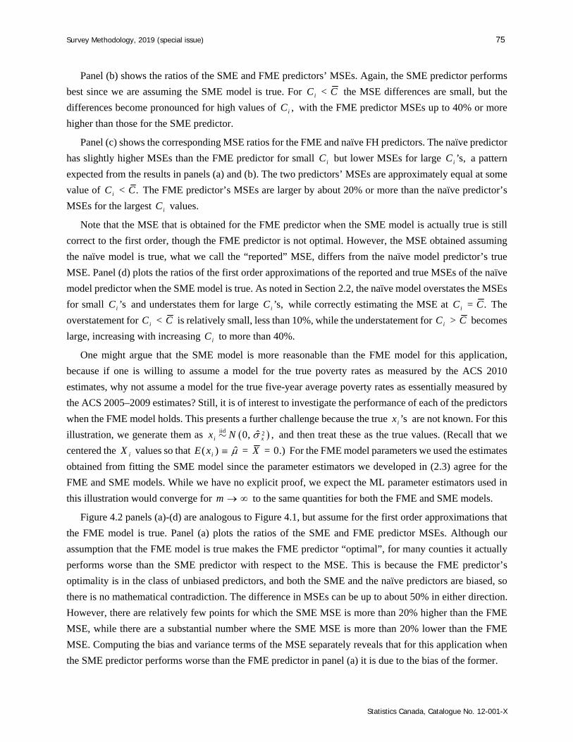
Survey Methodology, 2019 (special issue) 75
Statistics Canada, Catalogue No. 12-001-X
Panel (b) shows the ratios of the SME and FME predictors’ MSEs. Again, the SME predictor performs
best since we are assuming the SME model is true. For <iC C the MSE differences are small, but the
differences become pronounced for high values of ,iC with the FME predictor MSEs up to 40% or more
higher than those for the SME predictor.
Panel (c) shows the corresponding MSE ratios for the FME and naïve FH predictors. The naïve predictor
has slightly higher MSEs than the FME predictor for small iC but lower MSEs for large ’s,iC a pattern
expected from the results in panels (a) and (b). The two predictors’ MSEs are approximately equal at some
value of < .iC C The FME predictor’s MSEs are larger by about 20% or more than the naïve predictor’s
MSEs for the largest iC values.
Note that the MSE that is obtained for the FME predictor when the SME model is actually true is still
correct to the first order, though the FME predictor is not optimal. However, the MSE obtained assuming
the naïve model is true, what we call the “reported” MSE, differs from the naïve model predictor’s true
MSE. Panel (d) plots the ratios of the first order approximations of the reported and true MSEs of the naïve
model predictor when the SME model is true. As noted in Section 2.2, the naïve model overstates the MSEs
for small ’siC and understates them for large ’s,iC while correctly estimating the MSE at = .iC C The
overstatement for <iC C is relatively small, less than 10%, while the understatement for >iC C becomes
large, increasing with increasing iC to more than 40%.
One might argue that the SME model is more reasonable than the FME model for this application,
because if one is willing to assume a model for the true poverty rates as measured by the ACS 2010
estimates, why not assume a model for the true five-year average poverty rates as essentially measured by
the ACS 2005–2009 estimates? Still, it is of interest to investigate the performance of each of the predictors
when the FME model holds. This presents a further challenge because the true ’six are not known. For this
illustration, we generate them as iid 2ˆ0, ,i xx N and then treat these as the true values. (Recall that we
centered the iX values so that ˆ( ) = = 0.)iE x X For the FME model parameters we used the estimates
obtained from fitting the SME model since the parameter estimators we developed in (2.3) agree for the
FME and SME models. While we have no explicit proof, we expect the ML parameter estimators used in
this illustration would converge for m to the same quantities for both the FME and SME models.
Figure 4.2 panels (a)-(d) are analogous to Figure 4.1, but assume for the first order approximations that
the FME model is true. Panel (a) plots the ratios of the SME and FME predictor MSEs. Although our
assumption that the FME model is true makes the FME predictor “optimal”, for many counties it actually
performs worse than the SME predictor with respect to the MSE. This is because the FME predictor’s
optimality is in the class of unbiased predictors, and both the SME and the naïve predictors are biased, so
there is no mathematical contradiction. The difference in MSEs can be up to about 50% in either direction.
However, there are relatively few points for which the SME MSE is more than 20% higher than the FME
MSE, while there are a substantial number where the SME MSE is more than 20% lower than the FME
MSE. Computing the bias and variance terms of the MSE separately reveals that for this application when
the SME predictor performs worse than the FME predictor in panel (a) it is due to the bias of the former.

76 Bell et al.: Measurement error in small area estimation: Functional versus structural versus naïve models
Statistics Canada, Catalogue No. 12-001-X
Figure 4.2 First order approximations of MSE and bias squared ratios for the U.S. county school-age children
in poverty model when the FME model is true, plotted against iC or .ix Panels (a)-(c) show the ratios of the true MSEs of the SME and FME, SME and naïve, and FME and naïve models, respectively. Panel (d) shows the ratios of the reported MSEs and the true MSEs of the naïve model. Panel (e) shows the ratios of the biases squared of the SME and naïve models. All panels plot the ratios against iC except panel (f), which plots the ratio of the true MSEs of the SME and naïve models against .ix The vertical lines mark C or ,x as appropriate.
Panel (b) of Figure 4.2 plots ratios of the MSEs of the SME and naïve predictors against .iC It shows
that when the FME model is true, the SME predictor sometimes performs better and sometimes performs
worse than the naïve predictor in terms of MSE. The same statement can be made about the functional and
naïve predictors based on panel (c), which shows the ratios of the FME and naïve MSEs plotted against .iC
However, as iC increases beyond C the FME MSE is almost always higher than the naïve predictor’s
MSE.
1.4
1.0
0.6
(a) SME MSE / FME MSE (b) SME MSE / naïve FH MSE
1e‐05 5e‐05 5e‐04 5e‐03 1e‐05 5e‐05 5e‐04 5e‐03
C(i) C(i)
1.4
1.0
0.6
1.2
1.1
1.0
0.9
(c) FME MSE / naïve FH MSE (d) naïve FH reported / true MSE
1e‐05 5e‐05 5e‐04 5e‐03 1e‐05 5e‐05 5e‐04 5e‐03
C(i) C(i)
1.0
0.8
0.6
12
8
4
0
(e) SME bias squared / naïve FH bias squared (f) SME MSE / naïve FH MSE
1e‐05 5e‐05 5e‐04 5e‐03 ‐0.2 ‐0.1 0.0 0.1 0.2
C(i) x(i)
1.4
1.0
0.6
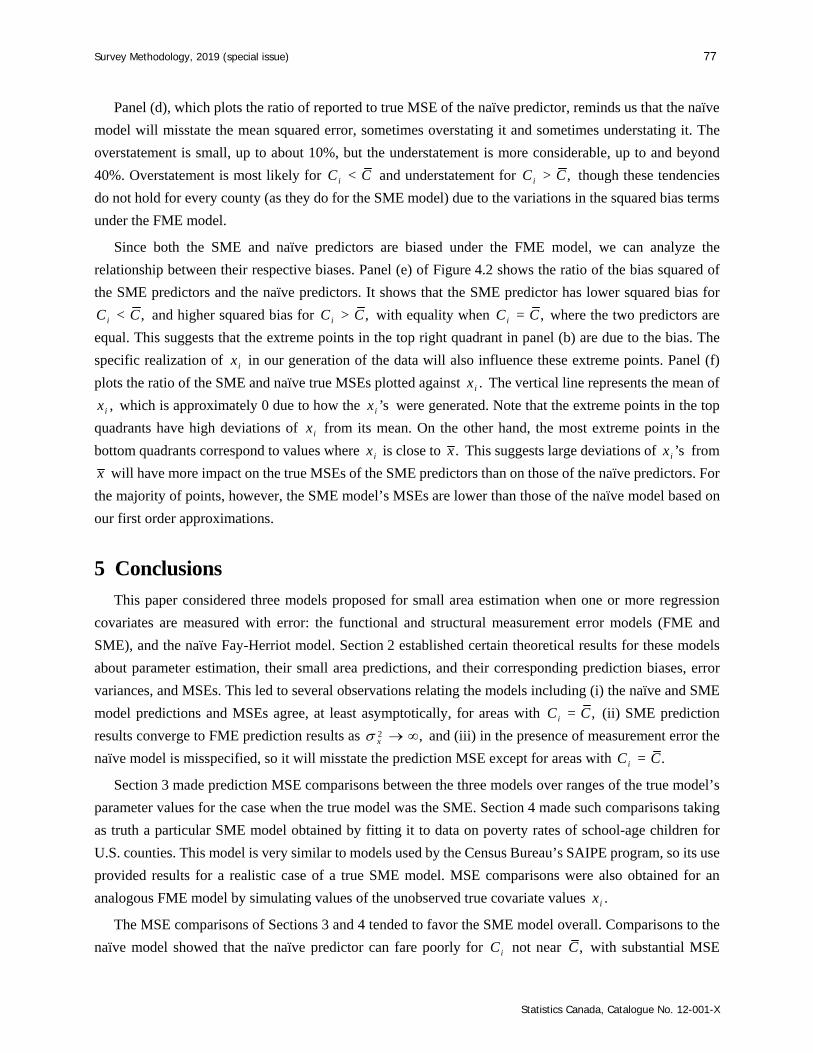
Survey Methodology, 2019 (special issue) 77
Statistics Canada, Catalogue No. 12-001-X
Panel (d), which plots the ratio of reported to true MSE of the naïve predictor, reminds us that the naïve
model will misstate the mean squared error, sometimes overstating it and sometimes understating it. The
overstatement is small, up to about 10%, but the understatement is more considerable, up to and beyond
40%. Overstatement is most likely for <iC C and understatement for > ,iC C though these tendencies
do not hold for every county (as they do for the SME model) due to the variations in the squared bias terms
under the FME model.
Since both the SME and naïve predictors are biased under the FME model, we can analyze the
relationship between their respective biases. Panel (e) of Figure 4.2 shows the ratio of the bias squared of
the SME predictors and the naïve predictors. It shows that the SME predictor has lower squared bias for
< ,iC C and higher squared bias for > ,iC C with equality when = ,iC C where the two predictors are
equal. This suggests that the extreme points in the top right quadrant in panel (b) are due to the bias. The
specific realization of ix in our generation of the data will also influence these extreme points. Panel (f)
plots the ratio of the SME and naïve true MSEs plotted against .ix The vertical line represents the mean of
,ix which is approximately 0 due to how the ’six were generated. Note that the extreme points in the top
quadrants have high deviations of ix from its mean. On the other hand, the most extreme points in the
bottom quadrants correspond to values where ix is close to .x This suggests large deviations of ’six from
x will have more impact on the true MSEs of the SME predictors than on those of the naïve predictors. For
the majority of points, however, the SME model’s MSEs are lower than those of the naïve model based on
our first order approximations.
5 Conclusions
This paper considered three models proposed for small area estimation when one or more regression
covariates are measured with error: the functional and structural measurement error models (FME and
SME), and the naïve Fay-Herriot model. Section 2 established certain theoretical results for these models
about parameter estimation, their small area predictions, and their corresponding prediction biases, error
variances, and MSEs. This led to several observations relating the models including (i) the naïve and SME
model predictions and MSEs agree, at least asymptotically, for areas with = ,iC C (ii) SME prediction
results converge to FME prediction results as 2 ,x and (iii) in the presence of measurement error the
naïve model is misspecified, so it will misstate the prediction MSE except for areas with = .iC C
Section 3 made prediction MSE comparisons between the three models over ranges of the true model’s
parameter values for the case when the true model was the SME. Section 4 made such comparisons taking
as truth a particular SME model obtained by fitting it to data on poverty rates of school-age children for
U.S. counties. This model is very similar to models used by the Census Bureau’s SAIPE program, so its use
provided results for a realistic case of a true SME model. MSE comparisons were also obtained for an
analogous FME model by simulating values of the unobserved true covariate values .ix
The MSE comparisons of Sections 3 and 4 tended to favor the SME model overall. Comparisons to the
naïve model showed that the naïve predictor can fare poorly for iC not near ,C with substantial MSE
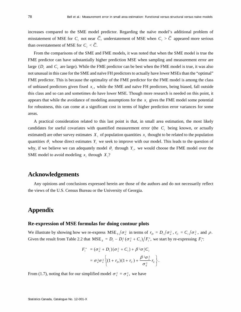
78 Bell et al.: Measurement error in small area estimation: Functional versus structural versus naïve models
Statistics Canada, Catalogue No. 12-001-X
increases compared to the SME model predictor. Regarding the naïve model’s additional problem of
misstatement of MSE for iC not near ,C understatement of MSE when >iC C appeared more serious
than overstatement of MSE for < .iC C
From the comparisons of the SME and FME models, it was noted that when the SME model is true the
FME predictor can have substantially higher prediction MSE when sampling and measurement error are
large ( iD and iC are large). While the FME predictor can be best when the FME model is true, it was also
not unusual in this case for the SME and naïve FH predictors to actually have lower MSEs than the “optimal”
FME predictor. This is because the optimality of the FME predictor for the FME model is among the class
of unbiased predictors given fixed ,ix while the SME and naïve FH predictors, being biased, fall outside
this class and so can and sometimes do have lower MSE. Though more research is needed on this point, it
appears that while the avoidance of modeling assumptions for the ix gives the FME model some potential
for robustness, this can come at a significant cost in terms of higher prediction error variances for some
areas.
A practical consideration related to this last point is that, in small area estimation, the most likely
candidates for useful covariates with quantified measurement error (the iC being known, or actually
estimated) are other survey estimates iX of population quantities ix thought to be related to the population
quantities i whose direct estimates iY we seek to improve with our model. This leads to the question of
why, if we believe we can adequately model i through ,iY we would choose the FME model over the
SME model to avoid modeling ix through ?iX
Acknowledgements
Any opinions and conclusions expressed herein are those of the authors and do not necessarily reflect
the views of the U.S. Census Bureau or the University of Georgia.
Appendix Re-expression of MSE formulas for doing contour plots
We illustrate by showing how we re-express 2MSE S u in terms of 2= ,D i ur D 2= ,C i xr C and .
Given the result from Table 2.2 that 2 2 *MSE = ,S i i x i iD D C F we start by re-expressing :iF
* 2 2 2 2
2 22 2
2
=
= 1 1 .
i u i x i x i
xu x D C C
u
F D C C
r r r
From (1.7), noting that for our simplified model 2 2= ,v x we have

Survey Methodology, 2019 (special issue) 79
Statistics Canada, Catalogue No. 12-001-X
2 4 2 222
2 2 2 2 2 2 2
2 2 2
2 2
= corr , = =
:= =1
x xi i
u x x u x
x
u
x
r
which implies that * 2 2= 1 1 .i u x D C CF r r r r Then
2 2 22
2 2 2
2
2
1MSE =
1 1
MSE 1= .
1 1
i u i x iS u
u u x D C C
S D CD
u D C C
D D C
r r r r
r rr
r r r r
References
Arima, S., Bell, W.R., Datta, G.S., Franco, C. and Liseo, B. (2017). Multivariate Fay-Herriot Bayesian estimation of small area means under functional measurement error. Journal of the Royal Statistical Society A, 180, 1191-1209, DOI:10.1111/rssa.12321.
Arima, S., Datta, G.S. and Liseo, B. (2012). Objective Bayesian analysis of a measurement error small area model. Bayesian Analysis, 7, 363-384.
Arima, S., Datta, G.S. and Liseo, B. (2015). Bayesian estimators for small area models when auxiliary information is measured with error. Scandinavian Journal of Statistics, 42, 518-529.
Arima, S., Datta, G.S. and Liseo, B. (2016). Accounting for measurement error in covariates in SAE: An overview. Analysis of Poverty Data by Small Area Estimation, (Ed., M. Pratesi), West Sussex, UK: Wiley, Chapter 8, 151-170.
Bell, W.R., Basel, W.W., Cruse, C., Dalzell, L., Maples, J.J., O’Hara, B. and Powers, D. (2007). Use of ACS data to produce SAIPE model-based estimates of poverty for counties. Unpublished technical paper available at https://www.census.gov/library/working-papers/2007/demo/bell-01.html.
Bell, W.R., Basel, W.W. and Maples, J.J. (2016). An overview of the U.S. Census Bureau’s small area income and poverty estimates program. Analysis of Poverty Data by Small Area Estimation, (Ed., M. Pratesi), West Sussex, UK: Wiley, Chapter 19, 349-378.
Bell, W.R., Chung, H.C., Datta, G. and Franco, C. (2018). Measurement error in small area estimation: Functional versus structural versus naïve models. Research Report RRS2018-06, Center for Statistical Research and Methodology, U.S. Census Bureau, available at https://www.census.gov/srd/ papers/pdf/RRS2018-06.pdf.
Buonaccorsi, J.P. (2010). Measurement Error: Models, Methods, and Applications. Boca Raton: Chapman and Hall/CRC Press.
Datta, G.S., Delaigle, A., Hall, P. and Wang, L. (2018). Semi-parametric prediction intervals in small areas when auxiliary data are measured with error. Statistica Sinica, 28, 2309-2335, DOI: 10.5705/ss.202016.0416.

80 Bell et al.: Measurement error in small area estimation: Functional versus structural versus naïve models
Statistics Canada, Catalogue No. 12-001-X
Datta, G.S., Rao, J.N.K. and Torabi, M. (2010). Pseudo-empirical Bayes estimation of small area means under a nested error linear regression model with functional measurement errors. Journal of Statistical Planning and Inference, 250, 2952-2962.
Fay, R.E., and Herriot, R.A. (1979). Estimates of income for small places: An application of James-Stein
procedure to census data. Journal of the American Statistical Association, 74, 269-277. Franco, C., and Bell, W.R. (2013). Applying bivariate binomial/logit normal models to small area
estimation. Proceedings of the American Statistical Association, Section on Survey Research Methods, 690-702, URL http://ww2.amstat.org/sections/srms/Proceedings/.
Fuller, W.A. (1987). Measurement Error Models. New York: John Wiley & Sons, Inc. Ghosh, M., and Sinha, K. (2007). Empirical Bayes estimation in finite population sampling under functional
measurement error models. Journal of Statistical Planning and Inference, 137, 2759-2773. Ghosh, M., Sinha, K. and Kim, D. (2006). Empirical and hierarchical Bayesian estimation in finite
population sampling under structural measurement error models. Scandinavian Journal of Statistics, 33, 591-608.
Huang, E.T., and Bell, W.R. (2012). An empirical study on using previous American Community Survey
data versus Census 2000 data in SAIPE models for poverty estimates. Research Report Number RRS2012-4, Center for Statistical Research and Methodology, U.S. Census Bureau, URL https://www.census.gov/srd/papers/pdf/rrs2012-04.pdf.
R Core Team (2016). R: A Language and Environment for Statistical Computing. Vienna: R Foundation for
Statistical Computing. URL https://www.R-project.org/. Theil, H. (1971). Principles of Econometrics. New York: John Wiley & Sons, Inc. Torabi, M., Datta, G.S. and Rao, J.N.K. (2009). Empirical Bayes estimation of small area means under
nested error linear regression model with measurement errors in the covariates. Scandinavian Journal of Statistics, 36, 355-368.
U.S. Census Bureau (2014). American Community Survey Design and Methodology (version 2.0, January
2014), URL https://www.census.gov/programs-surveys/acs/methodology.html. Wolter, K.M. (1985). Introduction to Variance Estimation. New York: Springer-Verlag. Ybarra, L.M.R., and Lohr, S.L. (2008). Small area estimation when auxiliary information is measured with
error. Biometrika, 95, 919-931.
Survey Methodology, 2019 (special issue) 81 Vol. 45, No. 1, pp. 81-99 Statistics Canada, Catalogue No. 12-001-X
1. Zhanshou Chen, School of Mathematics and Statistics, Qinghai Normal University, Xining 810008, P.R. China. E-mail:
[email protected]; Jiahua Chen and Qiong Zhang, Department of Statistics, University of British Columbia, Vancouver, BC, Canada.
Small area quantile estimation via spline regression and empirical likelihood
Zhanshou Chen, Jiahua Chen and Qiong Zhang1
Abstract
This paper studies small area quantile estimation under a unit level non-parametric nested-error regression model. We assume the small area specific error distributions satisfy a semi-parametric density ratio model. We fit the non-parametric model via the penalized spline regression method of Opsomer, Claeskens, Ranalli, Kauermann and Breidt (2008). Empirical likelihood is then applied to estimate the parameters in the density ratio model based on the residuals. This leads to natural area-specific estimates of error distributions. A kernel method is then applied to obtain smoothed error distribution estimates. These estimates are then used for quantile estimation in two situations: one is where we only have knowledge of covariate power means at the population level, the other is where we have covariate values of all sample units in the population. Simulation experiments indicate that the proposed methods for small area quantiles estimation work well for quantiles around the median in the first situation, and for a broad range of the quantiles in the second situation. A bootstrap mean square error estimator of the proposed estimators is also investigated. An empirical example based on Canadian income data is included.
Key Words: Small area quantile; Penalized spline; Empirical likelihood; Density ratio model; Nested-error regression
model.
1 Introduction
Sample surveys are widely used to obtain information about totals, means, medians and other quantities
of finite populations. Likewise, similar information on sub-populations such as individuals in specific areas
and socio-demographic groups are also of interest. Often, a survey is designed to collect information of
interest at the population level but leads to insufficient direct information on sub-populations. Because of
this, estimating sub-population parameters with satisfactory precision and evaluating their accuracy pose
serious challenges to statisticians. Statisticians must resort to suitable models to pool the information across
small areas in order to properly estimate parameters for small areas when only small samples or no samples
in these areas are available from the sample survey.
Research on small area estimation has received increased attention from both public and private sectors.
As historical remarks, we refer to Fay and Herriot (1979), Battese, Harter and Fuller (1988), Prasad and Rao
(1990), and Lahiri and Rao (1995) among many others. For a general review of the developments in small
area estimation, we refer to Pfeffermann (2002) and Pfeffermann (2013) and the books of Rao (2003) and
Rao and Molina (2015). See also Jiang and Lahiri (2006a), Jiang and Lahiri (2006b) and Jiang (2010) for
recent publications.
Compared to quantiles, there are relatively more research activities on estimating small area means.
Studies on small area quantile estimation are gaining ground. The M-quantile approach of Chambers and
Tzavidis (2006) has achieved substantial success. This approach uses the M-quantile approach to

82 Chen, Chen and Zhang: Small area quantile estimation via spline regression and empirical likelihood
Statistics Canada, Catalogue No. 12-001-X
characterize the conditional distributions of the response variable y given covariates .x This information
is then used to predict unobserved response values based on which the small area population distributions
are estimated. Small area quantile estimation is a natural and welcome side-benefit. See Tzavidis and
Chambers (2005), Pratesi, Ranalli and Salvati (2008), Tzavidis, Salvati and Pratesi (2008), and Salvati,
Tzavidis and Pratesi (2012) for these developments.
Another approach for small area quantile estimation is proposed by Molina (2010). Let s and r be the
sets of sampled and non-sampled units in a survey and sy and ry be vectors of corresponding response
values. Under a parametric assumption on the joint distribution of sy and ry (or the transformed responses)
they proposed to work out the conditional distribution of ry given sy (and other information). After having
the joint distribution and therefore the conditional distribution properly estimated, they suggested sampling
from the estimated conditional distribution to create an artificial but complete population with unobserved
ry filled up. The population distribution is estimated based on the completed population. This approach
works well for estimating small area means and quantiles. Other methods we are aware of include Tzavidis,
Marchetti and Chambers (2010), Chaudhuri and Ghosh (2011) and Chen and Liu (2018). Tzavidis et al.
(2010) proposed a general framework for robust small area estimation, based on representing a small area
estimator as a function of a predictor of this small area cumulative distribution function. Chaudhuri and
Ghosh (2011) proposed an empirical likelihood based Bayesian method. Chen and Liu (2018) proposed an
approach for populations admitting a nested-error linear regression model combined with error distributions
satisfying a semi-parametric density ratio model (DRM). Simulations indicate that the DRM-based method
stands out when the error distributions are skewed.
In this paper, we are interested in the situation where the regression function is not linear, although the
nested-error regression model remains appropriate similar to Opsomer et al. (2008). Clearly, methods
derived under linear models may lead to substantial bias if the linearity assumption is violated. To reduce
the potential risk of serious bias, Opsomer et al. (2008) proposed an Empirical Best Linear Unbiased
Prediction (EBLUP) for the small area means under a non-parametric regression model via penalized splines
(P-splines); Jiang, Ngueyen and Rao (2010) developed an adaptive fence approach employing a non-
parametric model selection technique; Sperlich and José Lombardía (2010) used the local polynomial
inference method in the context of small area estimation; Rao, Sinha and Dumitrescu (2014) proposed a
robust EBLUP under a P-splines approximated mixed model; Torabi and Shokoohi (2015) proposed a
unified analysis of both discrete and continuous responses under P-spline regression models.
We follow their lead and extend their results to allow non-normal error distributions in the nested-error
non-parametric regression model. More specifically, we assume the nested-error non-parametric regression
model but relax the small area error distribution assumption from normal to a flexible semi-parametric
DRM. We use the P-splines regression approach of Opsomer et al. (2008) to fit the nonlinear regression.
Empirical likelihood is then applied to estimate the parameters in the DRM based on the residuals. This
leads to natural area specific error distribution estimation. A kernel method is then applied to obtain
Survey Methodology, 2019 (special issue) 83
Statistics Canada, Catalogue No. 12-001-X
smoothed estimates of error distributions and small area quantiles. We construct quantile estimates in two
situations: one is where we have knowledge of only covariate power means at the population level, the other
is where we have covariate values of all sample units in the population. Our approach should inherit the
merits of working under a non-parametric regression model, and gain from avoiding a parametric error
distribution assumption. The resulting small area quantile estimates are hence more robust. Simulations
indicate that when the regression function is approximately linear, the performance of the proposed
approach is competitive. The proposed approach outperforms when the regression relationship is quadratic
or exponential.
The rest of the paper is organized as follows. Section 2 introduces the model and assumptions. Section 3
presents the proposed approach. Section 4 proposes a bootstrap procedure for estimating mean squared
errors. In Section 5, we use Monte Carlo methods to evaluate the performance of the proposed method and
compare it with some existing methods. An application example is reported in Section 6. Section 7 contains
some concluding remarks.
2 Model and assumptions
Consider a finite population containing =0
=m
iiN N sample units partitioned into 1m small areas
, : = 1, 2, , ,ij ij ix y j N = 0, 1, , .i m Consider a nested-error non-parametric regression model
with one covariate:
0= ,ij ij i ijy m x v (2.1)
where ijx is an auxiliary variable, iv denotes an area-specific random effect and ij are random errors. The
regression function 0m is unspecified, but can be approximated sufficiently well by a spline function
0 0 1=1
; , = .K
ppp k k
k
m x x x x β γ (2.2)
Here p is the degree of the spline, =p px x when > 0x and 0 otherwise, , = 1, ,k k K are a set of
fixed constants called knots, 0= , , p β is a coefficient vector of the parametric portion of the
model, and 1= , , K γ is the vector of spline coefficients, K is the number of spline knots. If knot
locations cover the range of x and K is sufficiently large, the class of P-spline (2.2) can approximate any
smooth function 0m with a high degree of accuracy, even with a small p (Boor, 2001). Ruppert, Wand
and Carroll (2003) recommended using the number of spline knots K as the minimum of 40 and the number
of unique ’sx divided by 4.
We assume that a random sample from the population is obtained under an uninformative sampling plan
such that (2.1) remains valid for the sampled units. Our immediate task is to fit this model based on the
sampled data and we follow the approach of Opsomer et al. (2008). For ease of presentation, we first
introduce some matrix notation. Let in be the number of units sampled from small area .i The response

84 Chen, Chen and Zhang: Small area quantile estimation via spline regression and empirical likelihood
Statistics Canada, Catalogue No. 12-001-X
values from the thi area will be denoted as 1 2= , , , .ii i i iny y y y We then pile them up to form the
response vector of length :n 0 1= , , , .n m Y y y y We similarly define i and n for error term. We use
0= , , mv v v for area specific random effects and create a matrix D such that
0 10 1= ( , , , )
mn n m nv v v Dv 1 1 1
with k1 being a length k vector of 1’s. We further construct matrices nX and nZ so that their rows are
made up of
1= 1, , , , = , ,p pp
ij ij ij ij ij ij Kx x x x
x z
in a proper order. With these matrices and vectors, the data in the sample under model (2.1) are connected
by
= .n n n n Y X β Z γ Dv (2.3)
Opsomer et al. (2008) fitted this model under the assumption that the components of ,γ of v and are
all independent and identically normally distributed with variances 2 , 2v and 2 respectively. The
solutions to the fit are given by
1
11 1
1
ˆ ˆ ˆ= ,
ˆˆ ˆˆ = ,
ˆ ˆ ˆ= ,
ˆˆ ˆˆ =
n n v
v n n
n n n n
n n n
V Z Σ Z DΣ D Σ
v Σ D V Y X β
β X V X X V Y
γ Σ Z V Y X β
where ˆ ˆ ˆ, ,v Σ Σ Σ are restricted maximum likelihood estimates of the covariance matrices of ,γ v and ,
and V is the estimate of var .nV Y
Opsomer et al. (2008) then gave the empirical best linear unbiased predictor of the small area mean:
0 1ˆ ˆ ˆ ˆ ˆ ˆ= ,p
i i p i i iY X X v z γ (2.4)
where , , pi iX X are the means of the powers of population units ijx in area ,i i.e., 1
=1= iN
s si i ijj
X N x
for = 1, , ,s p and ˆiz γ stands for the true means of the spline basis functions over the small area .i
Clearly, the above discussion easily extends to non-parametric additive models with two or more covariates
(Lin and Zhang (1999), Ruppert et al. (2003) and Wood (2006)).
In this paper, we follow Opsomer et al. (2008) to get all the fitted values. For small area quantile
estimation, we remove the normality assumption on .ij Instead, we assume that their distributions iG u
satisfy a DRM so that for = 1, , ,i m
0log = ,i idG u dG u u q (2.5)
Survey Methodology, 2019 (special issue) 85
Statistics Canada, Catalogue No. 12-001-X
with a pre-specified basis function uq and an area-specific tilting parameter .i One may include = 0i
in the above equation by setting 0 = 0. We require the first element of uq to be one, so that the first
element of i is a normalization parameter. The DRM includes normal, Gamma, and many other
distribution families as special cases. Discussions about DRM can be found in Anderson (1979), Qin and
Zhang (1997), Kezioua and Leoni-Aubina (2008) and Chen and Liu (2013).
Equations (2.1), (2.2) and (2.5) together form the platform of this paper for small area quantile
estimation. Our work differs from Opsomer et al. (2008) in that we focus on small area quantile estimation
without a normality assumption on .iG At the same time, this paper differs from Chen and Liu (2018)
by postulating a non-parametric regression relationship between ijy and ijx instead of a linear one.
3 Proposed approach
For any 0, 1 , the th quantile of a distribution F is defined to be
= inf : .u F u
If F u is an estimate of ,F u its - quantile is naturally estimated by
ˆ ˆ= inf : .u F u (3.1)
Under the distributional assumption on ,ij we have
0
0
= ,
= .
ij ij ij i ij i
i ij i
P y u P u m x v x v
G u m x v
Hence, the population distribution of the thi small area is given by
10
=1
= .iN
i i i ij ij
F u N G u m x v
Once iG and 0m are suitably estimated, so will be the small area quantiles.
We follow the empirical likelihood idea of Chen and Liu (2018) for estimating .iG Suppose the
values of ij in the sample are known. Consider a candidate 0G of the form
0,
= ,ij iji j
G u p I u
where I is an indicator function and , =0 =1
= .im n
i j i j We hence have 0=ij ijp dG and under
DRM = expi st st i stdG p θ q for = 0, 1, ,i m which implies
,
= exp .i st i st sts t
G u p I u θ q (3.2)
By Owen (2001), we obtain the empirical likelihood function
86 Chen, Chen and Zhang: Small area quantile estimation via spline regression and empirical likelihood
Statistics Canada, Catalogue No. 12-001-X
0 1, , ,
, , , = = exp ,n m i ij ij i iji j i j i j
L G G G dG p θ q
where the parameter θ and ’sijp satisfy 0,ijp and for = 0, 1, , ,s m
,
exp = 1.ij s iji j
p θ q (3.3)
Note that we have used the convention 0 = 0θ for simpler presentation. Because 1 , , mG G are fully
determined by 1= , , m θ θ θ and 0 ,G we write the empirical log-likelihood as
0,
, = log .n ij i iji j ij
G p θ θ q
Maximizing 0, Gθ with respect to 0G under the constraints (3.3) results in fitted probabilities
1
1
=1
ˆ = 1 exp ( ) 1m
ij s s ijs
p n
θ q (3.4)
and the profile log EL
, =1 ,
= log 1 exp 1m
n s s ij i iji j s i j
θ θ q θ q
with 1 , , m being the solution to
,=1
exp 1= 0.
1 exp 1
i st
ms t
l l stl
θ q
θ q
Since the values of ij are not available, we replace them by the residuals obtained from fitting model
(2.1) under assumption (2.2):
0ˆˆ ˆˆ ˆ= ; ,ij ij ij iy m x v β γ
where
0 0 1=1
ˆ ˆ ˆˆ ˆˆˆ ( ; , ) = .K
ppp k k
k
m x x x x β γ (3.5)
Let ˆn θ be the log EL function n θ after ij are replaced by ˆ .ij We define the maximum EL
estimator of θ by ˆ ˆ= argmax nθ θ and estimate iG u by
,
ˆ ˆ ˆˆ= expi st i st sts t
G u p I u θ q (3.6)
with

Survey Methodology, 2019 (special issue) 87
Statistics Canada, Catalogue No. 12-001-X
1
1
=1
ˆˆ = 1 exp 1m
st l l stl
p n n n
θ q
and 0ˆ = 0.θ The R package drmdel can be used to compute θ and ˆ ijp which has 11 choices of basis
function .uq
Because iG u is discrete, the following kernel smoothed distribution ˆiG u leads to better quantile
estimation:
=1
ˆˆ ˆ= ,
inij
i ijj
uG u w
b
(3.7)
where the weights are chosen to be ˆ ˆˆ = ,ij i ij i ijw G G b is a bandwidth parameter, and is the
distribution function of standard normal. As suggested by Chen and Liu (2013), we choose
1/5 ˆˆ= 1.06 min , 1.34b n Q where is the standard deviation of the distribution ˆiG and Q is its
interquartile range.
In some applications, only population power means of covariates are known and can be used for
statistical inference. In other applications, covariates of all members of the population are known. This leads
two possible quantile estimates. In the first case, we estimate iF by
10 0
=1
ˆˆ ˆ ˆˆ ˆ ˆˆ ˆ= ; , ; , ,in
ai i i i ij i
j
F u n G u Y m x m x β γ β γ (3.8)
where we use 0ˆ ˆˆ ; ,im x β γ specified in (3.5).
When the census information about x is available, we estimate iF by
10
ˆˆ ˆ ˆ= ,i i
bi i ij i ij i
j s j r
F u N I y u G u m x v
(3.9)
where is and ir are sets of observed and unobserved units in small area .i The rest of the specifications are
the same as in (3.8).
The proposed estimates resemble those of Chen and Liu (2018) but we use a non-parametric regression.
Because collecting population power means of covariates is easier than collecting covariates values of all
units in the population ˆ aiF u is more broadly applicable than ˆ .b
iF u It is also computationally more
efficient. Because ˆ biF u uses covariate values of all units in the population, it should statistically
outperform when both are applicable.
4 Bootstrap estimation of the mean squared errors
The proposed small area quantile estimators are assembled with many intermediate steps. It is difficult
to analytically evaluate the variances or mean squared error (MSE) of such estimators. We follow others
88 Chen, Chen and Zhang: Small area quantile estimation via spline regression and empirical likelihood
Statistics Canada, Catalogue No. 12-001-X
(Sinha and Rao (2009), Tzavidis et al. (2010) and Chen and Liu (2018)) to develop a bootstrap procedure
as follows:
Step 1 Obtain estimates 2ˆ ˆ ˆ, , vβ γ and 0ˆ ˆˆ , ,m x β γ based on Model (2.1), and calculate ˆ
iG u as
in (3.7).
Step 2 Generate a bootstrap finite population * *= , , = 0, , , = 1, ,ij ij iH y x i m j N with
* * *0
ˆ ˆˆ= , , ,ij ij i ijy m x v β γ
where the bootstrap residuals *ij are sampled from CDF ˆ
iG u , and *iv are generated from
2ˆ0, .vN
Step 3 From the bootstrap population * ,H we select * =i in n sample units from small area i by
simple random sampling without replacement, and repeat it L times to get * , = 1, , .lh l L
For each sample * ,lh compute the estimates *ˆ a liF u and *ˆ b l
iF u as in (3.8) and (3.9)
respectively.
Step 4 Compute the empirical MSE estimator of as
2* 1 * *
=1
ˆmse = ,L
l
l
L
where * *ˆˆ =l lF u denotes any functional of *ˆ a lF u or *ˆ b lF and * *= F u
with *F u being the known CDF of the bootstrap populations.
Step 5 Repeat Steps 2 to 4, B times, and define the bootstrap MSE estimate as
1 *
=1
mse ,B
bb
B
where *mse b is the *mse calculated in the thb repetition.
The performance of the bootstrap MSE estimator will be examined and reported in the simulation
section.
5 Monte Carlo simulations
In this section, we use simulation to evaluate the performances of the proposed penalized spline
regression model based empirical likelihood estimators (PEL) and their MSE estimates. When only the
covariate population means are known the proposed estimators are compared with only the nested-error
linear regression model based empirical likelihood estimator (LEL) of Chen and Liu (2018), and the direct
estimator (DE). When covariate values are known for all sample units, the comparison is extended to also
include six estimators of Tzavidis et al. (2010), denoted as EBLUP/naïve, EBLUP/CD, EBLUP/RKM,
M-quantile/naïve, M-quantile/CD and M-quantile/RKM. Here, EBLUP/CD and M-quantile/CD denote the
EBLUP and M-quantile estimator are obtained based on the CDF proposed by Chambers and Dunstan

Survey Methodology, 2019 (special issue) 89
Statistics Canada, Catalogue No. 12-001-X
(1986), and corresponding estimators based on the CDF proposed by Rao, Kovar and Mantel (1990) write
as RKM.
Similar to Chen and Liu (2018), we must choose uq in the DRM. Two candidates are 1 = 1,u u q
and 2 = 1, sign .u u u q Some preliminary simulation results indicate that 1 = 1,u u q works
well for the P-splines fitted non-parametric regression model, but 2 uq does not. Instead, the choice of
* 22 = 1, ,u u u q leads to competitive performance. So, we use 1 uq and *
2 uq in our simulation.
Following Rao et al. (2014) and Torabi and Shokoohi (2015), we generated data from the following three
models:
2
A : = 1 ,
B: = 1 ,
C: = 1 0.5 exp .
ij ij i ij
ij ij ij i ij
ij ij ij i ij
y x v
y x x v
y x x v
They lead to linear, quadratic and exponential regression functions respectively. We set the number of small
areas to be 30 and area population sizes = 500 1 , = 0, 1, , 29.iN i i We generated covariate ijx
from 0, 1 .N Once ijx are generated, we treated them as fixed in the simulation. The area-specific random
effect iv were generated from 0, 1 ,N and the errors ij were generated from the following four
distributions.
2
i : 0, 1 ,
ii : 3 ,
iii : normal mixture 0.5 1, 1 0.5 1, 1 ,
iv : 0, , with 0.5, 2 , = 0, , 29.i i
N
t
N N
N U i
Distribution (ii) has a heavy tail, distributions (ii) and (iii) are symmetric, and distribution (iv) is
heteroscedastic.
We used = 1,000R repetitions in the simulation and drew random samples of size = 500n without
replacement from the population in each repetition. To avoid the possibility that some small areas have too
few sample units, we drew 60n units at the population level and allocated an additional 2 units in each
small area. We used R package mgcv for the REML method with default options for values of p and K
when fitting the P-spline function (2.4). We calculated estimates of the 5%, 25%, 50%, 75%, and 95% small
area quantiles denoted as DE, LEL1, LEL2, PEL1, PEL2, for direct estimator, estimators of Chen and Liu
(2018) and the proposed estimators using 1 q and 2 .q We report their average mean squared error
(AMSE) and absolute biases (ABIAS) defined below:
21
=0 =1
1 1 1
=0 =1 =1
ˆAMSE = 1 ,
ˆABIAS = 1 ,
m Rr r
i ii r
m R Rr r
i ii r r
R m
m R R
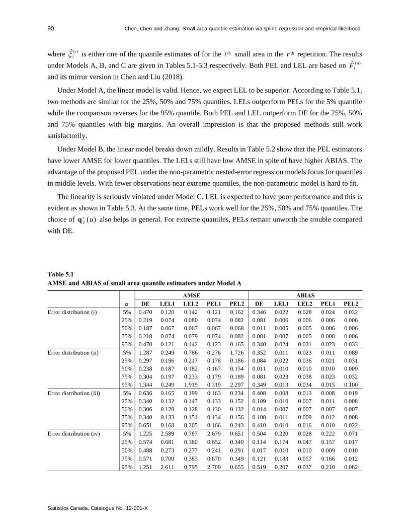
90 Chen, Chen and Zhang: Small area quantile estimation via spline regression and empirical likelihood
Statistics Canada, Catalogue No. 12-001-X
where ˆ ri is either one of the quantile estimates of for the thi small area in the thr repetition. The results
under Models A, B, and C are given in Tables 5.1-5.3 respectively. Both PEL and LEL are based on ˆ aiF
and its mirror version in Chen and Liu (2018).
Under Model A, the linear model is valid. Hence, we expect LEL to be superior. According to Table 5.1,
two methods are similar for the 25%, 50% and 75% quantiles. LELs outperform PELs for the 5% quantile
while the comparison reverses for the 95% quantile. Both PEL and LEL outperform DE for the 25%, 50%
and 75% quantiles with big margins. An overall impression is that the proposed methods still work
satisfactorily.
Under Model B, the linear model breaks down mildly. Results in Table 5.2 show that the PEL estimators
have lower AMSE for lower quantiles. The LELs still have low AMSE in spite of have higher ABIAS. The
advantage of the proposed PEL under the non-parametric nested-error regression models focus for quantiles
in middle levels. With fewer observations near extreme quantiles, the non-parametric model is hard to fit.
The linearity is seriously violated under Model C. LEL is expected to have poor performance and this is
evident as shown in Table 5.3. At the same time, PELs work well for the 25%, 50% and 75% quantiles. The
choice of *2 uq also helps in general. For extreme quantiles, PELs remain unworth the trouble compared
with DE.
Table 5.1 AMSE and ABIAS of small area quantile estimators under Model A
AMSE ABIAS
DE LEL1 LEL2 PEL1 PEL2 DE LEL1 LEL2 PEL1 PEL2
Error distribution (i) 5% 0.470 0.120 0.142 0.121 0.162 0.346 0.022 0.028 0.024 0.032 25% 0.219 0.074 0.080 0.074 0.082 0.081 0.006 0.006 0.006 0.006 50% 0.187 0.067 0.067 0.067 0.068 0.011 0.005 0.005 0.006 0.006 75% 0.218 0.074 0.079 0.074 0.082 0.081 0.007 0.005 0.008 0.006 95% 0.470 0.121 0.142 0.123 0.165 0.340 0.024 0.031 0.023 0.033
Error distribution (ii) 5% 1.287 0.249 0.786 0.276 1.726 0.352 0.011 0.023 0.011 0.089 25% 0.297 0.196 0.217 0.178 0.186 0.084 0.022 0.036 0.021 0.031 50% 0.238 0.187 0.182 0.167 0.154 0.011 0.010 0.010 0.010 0.009 75% 0.304 0.197 0.233 0.179 0.189 0.081 0.023 0.038 0.023 0.032 95% 1.344 0.249 1.919 0.319 2.297 0.349 0.013 0.034 0.015 0.100
Error distribution (iii) 5% 0.636 0.165 0.199 0.163 0.234 0.408 0.008 0.013 0.008 0.019 25% 0.340 0.132 0.147 0.133 0.152 0.109 0.010 0.007 0.011 0.008 50% 0.306 0.128 0.128 0.130 0.132 0.014 0.007 0.007 0.007 0.007 75% 0.340 0.133 0.151 0.134 0.156 0.108 0.011 0.009 0.012 0.008 95% 0.651 0.168 0.205 0.166 0.243 0.410 0.010 0.016 0.010 0.022
Error distribution (iv) 5% 1.225 2.589 0.787 2.679 0.651 0.504 0.220 0.028 0.222 0.071
25% 0.574 0.681 0.380 0.652 0.349 0.114 0.174 0.047 0.157 0.017
50% 0.488 0.273 0.277 0.241 0.291 0.017 0.010 0.010 0.009 0.010
75% 0.571 0.700 0.383 0.670 0.349 0.121 0.183 0.057 0.166 0.012
95% 1.251 2.611 0.795 2.709 0.655 0.519 0.207 0.037 0.210 0.082
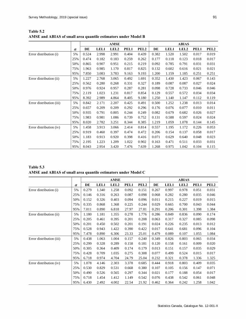
Survey Methodology, 2019 (special issue) 91
Statistics Canada, Catalogue No. 12-001-X
Table 5.2 AMSE and ABIAS of small area quantile estimators under Model B
AMSE ABIAS
DE LEL1 LEL2 PEL1 PEL2 DE LEL1 LEL2 PEL1 PEL2
Error distribution (i) 5% 0.524 2.998 2.991 0.404 0.439 0.382 1.520 1.502 0.017 0.019 25% 0.474 0.182 0.183 0.259 0.262 0.177 0.118 0.123 0.018 0.017 50% 0.865 0.907 0.951 0.215 0.219 0.092 0.785 0.791 0.031 0.031 75% 1.963 0.985 1.170 0.817 0.825 0.132 0.602 0.616 0.021 0.021 95% 7.850 3.083 3.783 9.163 9.193 1.200 1.159 1.185 0.251 0.251
Error distribution (ii) 5% 1.227 2.768 3.065 0.492 1.691 0.352 1.430 1.423 0.067 0.143 25% 0.562 0.280 0.268 0.331 0.327 0.189 0.087 0.087 0.027 0.024 50% 0.976 0.924 0.957 0.287 0.281 0.098 0.728 0.733 0.046 0.046 75% 2.119 1.023 1.231 0.817 0.854 0.129 0.557 0.572 0.034 0.034 95% 8.392 2.989 4.864 8.405 9.180 1.250 1.140 1.147 0.112 0.119
Error distribution (iii) 5% 0.842 2.171 2.207 0.425 0.491 0.500 1.252 1.238 0.013 0.014 25% 0.657 0.209 0.209 0.292 0.296 0.176 0.076 0.077 0.010 0.011 50% 0.935 0.791 0.805 0.244 0.249 0.082 0.679 0.682 0.026 0.027 75% 1.983 0.981 1.086 0.739 0.752 0.131 0.588 0.597 0.024 0.024 95% 8.020 2.782 3.251 8.344 8.385 1.219 1.059 1.078 0.144 0.145
Error distribution (iv) 5% 1.458 3.913 3.066 2.414 0.814 0.557 1.195 1.172 0.226 0.053 25% 0.919 0.460 0.397 0.474 0.472 0.206 0.154 0.137 0.058 0.017 50% 1.183 0.913 0.920 0.398 0.416 0.071 0.629 0.640 0.048 0.023 75% 2.195 1.223 1.209 1.022 0.902 0.163 0.471 0.511 0.033 0.031 95% 8.043 2.954 3.420 7.476 7.639 1.268 0.975 1.042 0.104 0.115
Table 5.3 AMSE and ABIAS of small area quantile estimators under Model C
AMSE ABIAS
DE LEL1 LEL2 PEL1 PEL2 DE LEL1 LEL2 PEL1 PEL2
Error distribution (i) 5% 0.279 1.340 1.258 0.092 0.151 0.267 0.997 0.978 0.051 0.031 25% 0.146 0.316 0.263 0.087 0.098 0.068 0.282 0.280 0.035 0.046 50% 0.152 0.326 0.403 0.094 0.096 0.011 0.215 0.227 0.019 0.015 75% 0.335 0.868 1.368 0.225 0.244 0.029 0.665 0.700 0.043 0.044 95% 7.011 0.890 6.818 27.97 27.81 0.291 0.206 0.301 1.398 1.384
Error distribution (ii) 5% 1.180 1.181 1.355 0.278 1.776 0.286 0.849 0.836 0.090 0.174 25% 0.205 0.461 0.395 0.201 0.208 0.063 0.317 0.327 0.085 0.098 50% 0.201 0.450 0.502 0.201 0.191 0.024 0.226 0.235 0.013 0.012 75% 0.528 0.943 1.422 0.390 0.422 0.017 0.641 0.681 0.096 0.104 95% 7.478 0.890 6.306 23.33 25.01 0.479 0.089 0.107 1.055 1.084
Error distribution (iii) 5% 0.438 1.063 1.004 0.157 0.240 0.349 0.826 0.803 0.065 0.034 25% 0.299 0.328 0.289 0.158 0.181 0.120 0.158 0.161 0.009 0.020 50% 0.305 0.364 0.409 0.174 0.179 0.013 0.151 0.157 0.035 0.029 75% 0.428 0.709 1.035 0.275 0.308 0.077 0.499 0.524 0.015 0.017 95% 6.718 0.974 4.704 24.79 25.04 0.232 0.321 0.378 1.336 1.325
Error distribution (iv) 5% 1.078 4.146 2.303 3.378 0.685 0.444 0.918 0.803 0.409 0.035 25% 0.530 0.829 0.531 0.668 0.380 0.107 0.105 0.156 0.147 0.071 50% 0.490 0.526 0.565 0.297 0.344 0.021 0.177 0.188 0.054 0.017 75% 0.718 1.454 1.412 1.149 0.542 0.076 0.438 0.542 0.061 0.048 95% 6.430 2.492 4.002 22.54 21.92 0.462 0.364 0.242 1.258 1.042
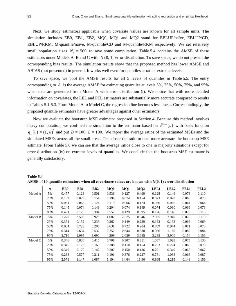
92 Chen, Chen and Zhang: Small area quantile estimation via spline regression and empirical likelihood
Statistics Canada, Catalogue No. 12-001-X
Next, we study estimators applicable when covariate values are known for all sample units. The
simulation includes EB0, EB1, EB2, MQ0, MQ1 and MQ2 stand for EBLUP/naïve, EBLUP/CD,
EBLUP/RKM, M-quantile/naïve, M-quantile/CD and M-quantile/RKM respectively. We set relatively
small population sizes = 500iN to save some computation. Table 5.4 contains the AMSE of these
estimators under Models A, B and C with 0, 1N error distribution. To save space, we do not present the
corresponding bias results. The simulation results show that the proposed method has lower AMSE and
ABIAS (not presented) in general. It works well even for quantiles at rather extreme levels.
To save space, we pool the AMSE results for all 5 levels of quantiles in Table 5.5. The entry
corresponding to iA is the average AMSE for estimating quantiles at levels 5%, 25%, 50%, 75%, and 95%
when data are generated from Model A with error distribution (i). We notice that with more detailed
information on covariates, the LEL and PEL estimators are substantially more accurate compared to results
in Tables 5.1-5.3. From Model A to Model C, the regression line becomes less linear. Correspondingly, the
proposed quantile estimators have greater advantages against other estimators.
Now we evaluate the bootstrap MSE estimator proposed in Section 4. Because this method involves
heavy computation, we confined the simulation to the estimator based on ˆ biF u with basis function
1 = 1,u u q and put = 100, = 100.B L We report the average ratios of the estimated MSEs and the
simulated MSEs across all the small areas. The closer the ratio to one, more accurate the bootstrap MSE
estimate. From Table 5.6 we can see that the average ratios close to one in majority situations except for
error distribution (iv) on extreme levels of quantiles. We conclude that the bootstrap MSE estimator is
generally satisfactory.
Table 5.4 AMSE of 10 quantile estimators when all covariance values are known with N(0, 1) error distribution
EB0 EB1 EB2 MQ0 MQ1 MQ2 LEL1 LEL2 PEL1 PEL2
Model A 5% 0.477 0.123 0.501 0.536 0.127 0.499 0.128 0.146 0.078 0.110 25% 0.139 0.073 0.154 0.198 0.074 0.154 0.073 0.078 0.065 0.073 50% 0.061 0.066 0.124 0.119 0.066 0.124 0.066 0.066 0.064 0.064 75% 0.145 0.074 0.149 0.204 0.074 0.149 0.074 0.080 0.066 0.073 95% 0.491 0.125 0.394 0.552 0.129 0.395 0.126 0.146 0.079 0.113
Model B 5% 1.270 2.500 0.928 1.682 2.575 0.946 2.965 2.949 0.079 0.110 25% 0.351 0.152 0.239 0.262 0.149 0.239 0.193 0.193 0.069 0.069 50% 0.834 0.723 0.285 0.631 0.722 0.284 0.899 0.944 0.071 0.073 75% 0.314 0.634 0.532 0.257 0.644 0.530 0.986 1.160 0.082 0.084 95% 3.710 2.095 3.690 4.209 2.059 3.685 3.235 3.900 0.154 0.156
Model C 5% 0.346 0.830 0.415 0.708 0.307 0.351 1.087 1.028 0.075 0.130 25% 0.345 0.173 0.169 0.388 0.110 0.154 0.263 0.224 0.066 0.075
50% 0.340 0.170 0.142 0.207 0.150 0.136 0.291 0.349 0.065 0.067
75% 0.288 0.577 0.211 0.191 0.376 0.227 0.731 1.088 0.068 0.087
95% 2.578 11.47 8.087 5.194 14.64 11.96 0.868 4.215 0.148 0.156
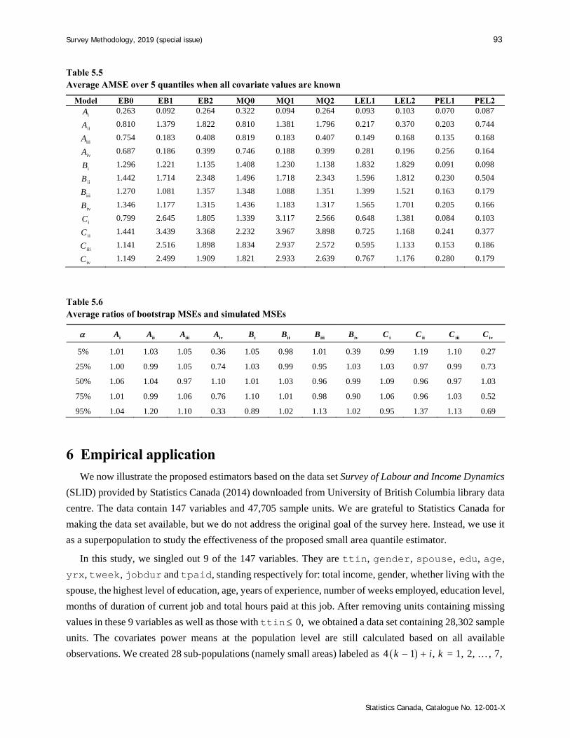
Survey Methodology, 2019 (special issue) 93
Statistics Canada, Catalogue No. 12-001-X
Table 5.5 Average AMSE over 5 quantiles when all covariate values are known
Model EB0 EB1 EB2 MQ0 MQ1 MQ2 LEL1 LEL2 PEL1 PEL2
iA 0.263 0.092 0.264 0.322 0.094 0.264 0.093 0.103 0.070 0.087
iiA 0.810 1.379 1.822 0.810 1.381 1.796 0.217 0.370 0.203 0.744
iiiA 0.754 0.183 0.408 0.819 0.183 0.407 0.149 0.168 0.135 0.168
ivA 0.687 0.186 0.399 0.746 0.188 0.399 0.281 0.196 0.256 0.164
iB 1.296 1.221 1.135 1.408 1.230 1.138 1.832 1.829 0.091 0.098
iiB 1.442 1.714 2.348 1.496 1.718 2.343 1.596 1.812 0.230 0.504
iiiB 1.270 1.081 1.357 1.348 1.088 1.351 1.399 1.521 0.163 0.179
ivB 1.346 1.177 1.315 1.436 1.183 1.317 1.565 1.701 0.205 0.166
iC 0.799 2.645 1.805 1.339 3.117 2.566 0.648 1.381 0.084 0.103
iiC 1.441 3.439 3.368 2.232 3.967 3.898 0.725 1.168 0.241 0.377
iiiC 1.141 2.516 1.898 1.834 2.937 2.572 0.595 1.133 0.153 0.186
ivC 1.149 2.499 1.909 1.821 2.933 2.639 0.767 1.176 0.280 0.179
Table 5.6 Average ratios of bootstrap MSEs and simulated MSEs
iA iiA iiiA ivA iB iiB iiiB ivB iC iiC iiiC ivC
5% 1.01 1.03 1.05 0.36 1.05 0.98 1.01 0.39 0.99 1.19 1.10 0.27
25% 1.00 0.99 1.05 0.74 1.03 0.99 0.95 1.03 1.03 0.97 0.99 0.73
50% 1.06 1.04 0.97 1.10 1.01 1.03 0.96 0.99 1.09 0.96 0.97 1.03
75% 1.01 0.99 1.06 0.76 1.10 1.01 0.98 0.90 1.06 0.96 1.03 0.52
95% 1.04 1.20 1.10 0.33 0.89 1.02 1.13 1.02 0.95 1.37 1.13 0.69
6 Empirical application
We now illustrate the proposed estimators based on the data set Survey of Labour and Income Dynamics
(SLID) provided by Statistics Canada (2014) downloaded from University of British Columbia library data
centre. The data contain 147 variables and 47,705 sample units. We are grateful to Statistics Canada for
making the data set available, but we do not address the original goal of the survey here. Instead, we use it
as a superpopulation to study the effectiveness of the proposed small area quantile estimator.
In this study, we singled out 9 of the 147 variables. They are ttin, gender, spouse, edu, age,
yrx, tweek, jobdur and tpaid, standing respectively for: total income, gender, whether living with the
spouse, the highest level of education, age, years of experience, number of weeks employed, education level,
months of duration of current job and total hours paid at this job. After removing units containing missing
values in these 9 variables as well as those with ttin 0, we obtained a data set containing 28,302 sample
units. The covariates power means at the population level are still calculated based on all available
observations. We created 28 sub-populations (namely small areas) labeled as 4 1 ,k i = 1, 2, , 7,k
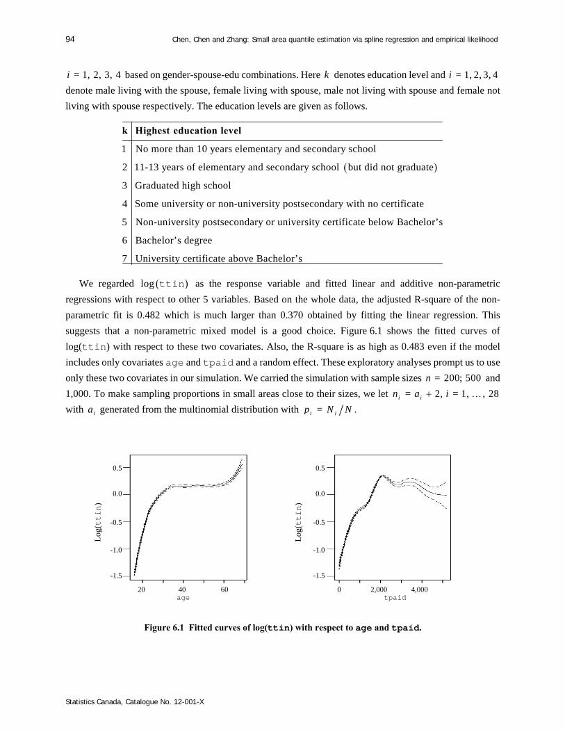
94 Chen, Chen and Zhang: Small area quantile estimation via spline regression and empirical likelihood
Statistics Canada, Catalogue No. 12-001-X
= 1, 2, 3, 4i based on gender-spouse-edu combinations. Here k denotes education level and = 1, 2, 3, 4i
denote male living with the spouse, female living with spouse, male not living with spouse and female not
living with spouse respectively. The education levels are given as follows.
No more than 10 years elementary and secondary school
11-13 years of elementary and secondary school but did not graduate
Graduated high school
Some u
1
2
3
4 niversity or non-universi
k Highest education level
ty postsecondary with no certificate
Non-university postsecondary or university certificate below Bachelor’s
Bachelor’s degree
University certificate above Bachel
5
6
7 or’s
We regarded log ttin as the response variable and fitted linear and additive non-parametric
regressions with respect to other 5 variables. Based on the whole data, the adjusted R-square of the non-
parametric fit is 0.482 which is much larger than 0.370 obtained by fitting the linear regression. This
suggests that a non-parametric mixed model is a good choice. Figure 6.1 shows the fitted curves of
log(ttin) with respect to these two covariates. Also, the R-square is as high as 0.483 even if the model
includes only covariates age and tpaid and a random effect. These exploratory analyses prompt us to use
only these two covariates in our simulation. We carried the simulation with sample sizes = 200; 500n and
1,000. To make sampling proportions in small areas close to their sizes, we let = 2, = 1, , 28i in a i
with ia generated from the multinomial distribution with = .i ip N N
Figure 6.1 Fitted curves of log(ttin) with respect to age and tpaid.
0.5
0.0
-0.5
-1.0
-1.5
Log
(ttin
)
0.5
0.0
-0.5
-1.0
-1.5
Log
(ttin
)
20 40 60 0 2,000 4,000 age tpaid

Survey Methodology, 2019 (special issue) 95
Statistics Canada, Catalogue No. 12-001-X
The simulated AMSE of 10 estimators based on 1,000 repetitions are reported in Table 6.1. We first
notice that both our PEL estimators outperform the other estimators, in general, indicating the advantage of
our non-parametric DRM based small area estimation technique. The PEL1 compared to PEL2 has the lower
AMSE for 5%, 25%, and 50% quantiles, but slightly higher AMSE for 75% and 95% quantiles indicating
the heteroscedasticity of data is not serious. Regardless the PEL estimators, we notice the LEL estimators
outperform other estimators for 5% quantile, and have similar performance for other quantiles. Increasing
the sample size reduces the AMSE of all estimators. Clearly, it is hard to estimate the 5% quantile with a
good precision because the data are skewed toward the left so there are few observations for estimating the
lower quantiles. Interestingly, LEL1 is not affected as much by the skewness. We feel that the kernel
smoothing step (3.7) is helpful here. Without this smoothing step, LEL1 would perform much worse.
Unreported simulations show that the ABIAS of all estimators decreases in general as the sample size
increases and this is most apparent for DE.
To check the performance of the proposed first estimator which using only covariate average
information. In Figures 6.2, we depict the 2.5%, 50%, and 97.5% quantiles of 1,000 small area median
estimates by the DE, LEL1, LEL2, PEL1, PEL2 with sample size = 200n with the true medians marked
by dots. The y-axis is the total income and x-axis is the education level. It is seen that the PEL2 boxes are
the shortest for most small areas.
Table 6.2 reports the bootstrap MSE estimates as well as the average ratios of bootstrap and simulated
MSEs of the small area median estimators based on ˆ aiF u and ˆ b
iF u with sample size = 200.n The
number of simulation repetition is 500 with basis function 1 = 1,u u q and = 100, = 100.B L We can
see the estimator ˆ aiF u has higher MSE than ˆ ,b
iF u and most average ratios close to one.
Table 6.1 AMSE of small area quantile estimators based on real data
EB0 EB1 EB2 MQ0 MQ1 MQ2 LEL1 LEL2 PEL1 PEL2
n = 200 5% 0.784 0.769 0.901 0.714 0.763 0.885 0.245 0.421 0.242 0.336
25% 0.107 0.256 0.488 0.102 0.261 0.467 0.115 0.131 0.097 0.152
50% 0.080 0.119 0.236 0.064 0.116 0.223 0.076 0.095 0.056 0.102
75% 0.122 0.100 0.142 0.085 0.102 0.138 0.085 0.076 0.069 0.068
95% 0.233 0.190 0.280 0.141 0.138 0.266 0.217 0.179 0.117 0.096
n = 500 5% 0.793 0.603 0.826 0.710 0.579 0.805 0.173 0.345 0.210 0.301
25% 0.072 0.110 0.207 0.076 0.119 0.197 0.069 0.127 0.063 0.091
50% 0.049 0.050 0.074 0.036 0.050 0.072 0.053 0.076 0.040 0.043
75% 0.108 0.044 0.060 0.055 0.046 0.058 0.054 0.047 0.046 0.043
95% 0.257 0.128 0.152 0.109 0.058 0.148 0.138 0.125 0.086 0.077
n = 1,000 5% 0.792 0.397 0.542 0.706 0.377 0.528 0.078 0.130 0.095 0.144
25% 0.054 0.056 0.098 0.066 0.067 0.095 0.041 0.043 0.038 0.056
50% 0.034 0.026 0.032 0.027 0.026 0.031 0.019 0.028 0.018 0.024
75% 0.102 0.024 0.030 0.043 0.026 0.030 0.037 0.033 0.019 0.023
95% 0.270 0.088 0.090 0.095 0.114 0.090 0.074 0.067 0.053 0.057

96 Chen, Chen and Zhang: Small area quantile estimation via spline regression and empirical likelihood
Statistics Canada, Catalogue No. 12-001-X
Table 6.2 Bootstrap MSE estimates and average ratios of the estimated and simulated MSEs
ˆ aiF u ˆ b
iF u
5% 25% 50% 75% 95% 5% 25% 50% 75% 95% MSE 0.542 0.196 0.117 0.098 0.165 0.204 0.093 0.068 0.062 0.102 Ratio 0.843 0.959 1.014 0.988 0.871 0.969 0.994 1.003 0.996 0.975
Figure 6.2 The bottom, middle and top lines of each bar denote 2.5%, 50% and 97.5% quantiles of 1,000 small area estimates of the total income. The dot in each bar denotes true small area median. Five bars in each cluster are formed by DE, LEL1, LEL2, PEL1, PEL2 estimates. Top two plots: male living (left) and not living (right) with spouse; Bottom two plots: female living (left) and not living (right) with spouse. Seven clusters in each plot correspond to 7 education levels.
1 2 3 4 5 6 7 1 2 3 4 5 6 7
Education Education
1 2 3 4 5 6 7 1 2 3 4 5 6 7
Education Education
150,000
100,000
50,000
0
100,000
75,000
50,000
25,000
0
160,000
120,000
80,000
40,000
90,000
60,000
30,000
I
ncom
e
Inc
ome
I
ncom
e
Inc
ome

Survey Methodology, 2019 (special issue) 97
Statistics Canada, Catalogue No. 12-001-X
7 Conclusion
We studied the small area quantile estimation under the nested-error non-parametric regression model
and a semi-parametric DRM assumption on error distributions. We proposed two quantile estimators based
on P-splines and empirical likelihood approach. Simulation results show that the proposed estimators are
robust and have respectable efficiency under both linear and non-parametric regression functions for mid-
range quantiles. The proposed approach can be extended to non-parametric regression models with multiple
covariates in principle, though it will lead to many more parameters to be estimated. This problem will be
investigated in a future work.
Acknowledgements
We thank Professors Simon Wood, Matt Wand, Mahmoud Torabi and Song Cai for their helpful
suggestions on R packages used in this paper. This work was supported by the National Natural Science
Foundation of China (No.11661067), Natural Science Foundation of Qinghai Province (No.2015-ZJ-
717,2019-ZJ-920), “Western Light” talent program of Chinese Academy of Science (2017) and the funding
through the Canadian Statistical Sciences Institute.
References
Anderson, J.A. (1979). Multivariate logistic compounds. Biometrika, 66, 17-26. Battese, G.E., Harter, R.M. and Fuller, W.A. (1988). An error-components model for prediction of county
crop areas using survey and satellite data. Journal of the American Statistical Association, 80, 28-36. Boor, C.D. (2001). A Practical Guide to Splines. New York: Springer. Chambers, R., and Dunstan, R. (1986). Estimating distribution functions from survey data. Biometrika, 73,
597-604. Chambers, R., and Tzavidis, N. (2006). M-quantile models for small area estimation. Biometrika, 93, 255-
268. Chaudhuri, S., and Ghosh, M. (2011). Empirical likelihood for small area estimation. Biometrika, 98, 473-
480. Chen, J., and Liu, Y. (2013). Quantile and quantile-function estimations under density ratio model. The
Annals of Statistics, 41, 1669-1692. Chen, J., and Liu, Y. (2018). Small area quantile estimation. International Statistics Review. In print.
arXiv:1705.10063. Fay, R.E., and Herriot, R.A. (1979). Estimates of income for small places: An application of James-Stein
procedures to census data. Journal of the American Statistical Association, 74, 269-277.

98 Chen, Chen and Zhang: Small area quantile estimation via spline regression and empirical likelihood
Statistics Canada, Catalogue No. 12-001-X
Jiang, J. (2010). Large Sample Techniques for Statistics. New York: Springer. Jiang, J., and Lahiri, P. (2006a). Estimation of finite population domain means: A model-assisted empirical
best prediction approach. Journal of the American Statistical Association, 101, 301-311. Jiang, J., and Lahiri, P. (2006b). Mixed model prediction and small area estimation. Test, 15, 1-96. Jiang, J., Ngueyen, T. and Rao, J.S. (2010). Fence method for nonparametric small area estimation. Survey
Methodology, 36, 1, 3-11. Paper available at https://www150.statcan.gc.ca/n1/en/pub/12-001-x/2010001/article/11244-eng.pdf.
Kezioua, A., and Leoni-Aubina, S. (2008). On empirical likelihood for semiparametric two-sample density
ratio models. Journal of Statistical Planning and Inference, 138, 915-928. Lahiri, P.S., and Rao, J.N.K. (1995). Robust estimation of mean squared error of small area estimators.
Journal of the American Statistical Association, 90, 758-766. Lin, X., and Zhang, D. (1999). Inference in generalized additive mixed models using smoothing splines.
Journal of the Royal Statistical Society, Series B, 61, 381-400. Molina, I., and Rao, J.N.K. (2010). Small area estimation of poverty indicators. The Canadian Journal of
Statistics, 38, 369-385. Opsomer, J.D., Claeskens, G., Ranalli, M.G., Kauermann, G. and Breidt, F.J. (2008). Non-parametric small
area estimation using penalized spline regression. Journal of the Royal Statistical Society: B, 70, 265-286.
Owen, A.B. (2001). Empirical Likelihood. New York: Chapman & Hall/CRC. Prasad, N.G.N., and Rao, J.N.K. (1990). The estimation of mean squared errors of small area estimators.
Journal of the American Statistical Association, 85, 163-171. Pfeffermann, D. (2002). Small area estimation-New developments in small area estimation. International
Statistical Review, 70, 125-143. Pfeffermann, D. (2013). New important developments in small area estimation. Statistical Science, 28, 40-
68. Pratesi, M., Ranalli, M.G. and Salvati, N. (2008). Semiparametric M-quantile regression for estimation for
estimating the proportion of acidic lakes in 8-digit HUCs of the Northeastern US. Environmetrics, 19, 687-701.
Qin, J., and Zhang, B. (1997). A goodness-of-fit test for logistic regression models based on case-control
data. Biometrika, 84, 609-618. Rao, J.N.K. (2003). Small Area Estimation. New York: John Wiley & Sons, Inc. Rao, J.N.K., Kovar, J.G. and Mantel, H.J. (1990). On estimating distribution functions and quantiles from
survey data using auxiliary information. Biometrika, 77, 365-375. Rao, J.N.K., and Molina, I. (2015). Small Area Estimation, 2nd Edition. New York: John Wiley & Sons, Inc.
Survey Methodology, 2019 (special issue) 99
Statistics Canada, Catalogue No. 12-001-X
Rao, J.N.K., Sinha, S.K. and Dumitrescu, L. (2014). Robust small area estimation under semi-parametric mixed models. The Canadian Journal of Statistics, 42, 126-141.
Ruppert, D., Wand, M.P. and Carroll, R.J. (2003). Semiparametric Regression. Cambridge University Press,
Cambridge. Salvati, N., Tzavidis, N. and Pratesi, M. (2012). Small area estimation via M-quantile geographically
weighted regression. Test, 21, 1-28. Sinha, S.K., and Rao, J.N.K. (2009). Robust small area estimation. The Canadian Journal of Statistics,
37(3), 381-399. Sperlich, S., and José Lombardía, M. (2010). Local polynomial inference for small area statistics:
Estimation, validation and prediction. Journal of Non-parametric Statistics, 22, 633-648. Statistics Canada (2014). Survey of labour and income dynamics, 2011. Access:
http://tinyurl.com/y2ys2zzs. Torabi, M., and Shokoohi, F. (2015). Non-parametric generalized linear mixed models in small area
estimation. The Canadian Journal of Statistics, 43, 82-96. Tzavidis, N., and Chambers, R. (2005). Bias adjusted estimation for small areas with M-quantile models.
Statistics in Transition, 7, 707-713. Tzavidis, N., Salvati, N. and Pratesi, M. (2008). M-quantile models with application to poverty mapping.
Statistical Methods and Applications, 17, 393-411. Tzavidis, N., Marchetti, S. and Chambers, R. (2010). Robust prediction of small area means and quantiles.
Australian and New Zealand Journal of Statistics, 52, 167-186. Wood, S.N. (2006). Generalized Additive Models: An Introduction with R. Boca Raton, Florida: Chapman
& Hall/CRC.


Survey Methodology, 2019 (special issue) 101 Vol. 45, No. 1, pp. 101-126 Statistics Canada, Catalogue No. 12-001-X
1. Michel A. Hidiroglou, Business Survey Methods, Statistics Canada, 22th Floor R.H. Coats Building, Ottawa, ON, K1A 0T6, Canada. E-mail:
[email protected]; Jean-François Beaumont, International Cooperation and Corporate Statistical Methods Division, Statistics Canada, 25th Floor R.H. Coats Building, Ottawa, ON, K1A 0T6, Canada; Wesley Yung, Business Survey Methods, Statistics Canada, 22th Floor R.H. Coats Building, Ottawa, ON, K1A 0T6, Canada.
Development of a small area estimation system at Statistics Canada
Michel A. Hidiroglou, Jean-François Beaumont and Wesley Yung1
Abstract
The demand for small area estimates by users of Statistics Canada’s data has been steadily increasing over recent years. In this paper, we provide a summary of procedures that have been incorporated into a SAS based production system for producing official small area estimates at Statistics Canada. This system includes: procedures based on unit or area level models; the incorporation of the sampling design; the ability to smooth the design variance for each small area if an area level model is used; the ability to ensure that the small area estimates add up to reliable higher level estimates; and the development of diagnostic tools to test the adequacy of the model. The production system has been used to produce small area estimates on an experimental basis for several surveys at Statistics Canada that include: the estimation of health characteristics, the estimation of under-coverage in the census, the estimation of manufacturing sales and the estimation of unemployment rates and employment counts for the Labour Force Survey. Some of the diagnostics implemented in the system are illustrated using Labour Force Survey data along with administrative auxiliary data.
Key Words: Small area estimation; Area level model; Unit level model; EBLUP; Hierarchical Bayes methods; Official
Statistics.
1 Introduction
Today’s data users are becoming more and more sophisticated and are asking for more data and at more
detailed levels. For National Statistical Offices (NSOs) facing declining response rates, producing data at
finer levels of detail is a particularly daunting challenge. Small area estimation techniques are one way that
can be considered to meet this demand to produce estimates for specified sub-populations or small areas. A
small area refers to a subgroup of the population for which the sample size is so small that direct estimates
are not reliable enough to be published. Examples of small areas include a geographical region (e.g., a
province, county, municipality, etc.), a demographic group (e.g., age by sex), a demographic group within
a geographic region or a detailed industry group. The demand for small area data has been recognized for
years (see Brackstone, 1987), but recently, it has greatly increased as noted in the spring 2014 report of the
Auditor General of Canada.
The study of small area estimation procedures has a long history at Statistics Canada, beginning in the
seventies with Singh and Tessier (1976) and Ghangurde and Singh (1977). Drew, Singh and Choudhry
(1982) proposed a sample dependent procedure to estimate employment characteristics below the provincial
level. Dick (1995) modeled net undercoverage for the 1991 Canadian Census of Population. The
development of a small area estimation system suited to Statistics Canada surveys is well-timed, as there is
now a great deal of literature written on the subject, including the books by Rao (2003) and Rao and Molina
(2015).
102 Hidiroglou et al.: Development of a small area estimation system at Statistics Canada
Statistics Canada, Catalogue No. 12-001-X
Four papers that have had a great impact in small area estimation (SAE) are Gonzalez and Hoza (1978),
Fay and Herriot (1979), Battese, Harter and Fuller (1988), and Prasad and Rao (1990). Gonzalez and Hoza
(1978) were among the first to propose small area estimation procedures (mainly synthetic estimation). Fay
and Herriot (1979) developed procedures to estimate income for small areas using the long form Census
Data. This method and its variants are among the most widely used procedures for producing small area
estimates through the integration of auxiliary data with direct survey estimates. Battese et al. (1988)
developed a small area procedure to estimate crop areas using survey and satellite data available for
individual units. Finally, Prasad and Rao (1990) derived a nearly unbiased estimator of the model-based
mean squared error for both the Fay-Herriot and Battese-Harter-Fuller estimators.
The statistical theory of model-based SAE is rather complex and much of the software available at
National Statistical Offices has been programmed on a one-time basis and, as such, is not appropriate in a
production environment. It was therefore decided to develop a system as it would be beneficial as a
production tool, as well as a learning tool for employees. At the time that this was decided, around 2006,
there existed computer programs developed by the EURAREA (2004) project for small area estimation.
However, this set of programs was no longer in development mode and did not represent the latest advances
in small area estimation. Therefore, a flexible small area estimation system that would address the needs of
producing small area estimates in production was developed at Statistics Canada. Some of the basic
requirements of this small area system included: allowing for both area and unit level models; incorporating
the sampling design in the estimation of the parameters of interest and the mean squared error; ensuring that
the small area estimates would add up to reliable higher level estimates (i.e., totals), and developing
diagnostic tools to test the adequacy of the models used for small area estimation. A prototype system,
written in SAS, was therefore developed by Estevao, Hidiroglou and You (2015) to reflect these
requirements. This prototype has been transformed into a production system that is currently used by
Statistics Canada.
The paper is organized as follows. Section 2 introduces the notation used in the article. Section 3
discusses the options available in the production system for the area level model and Empirical Best Linear
Unbiased Prediction (EBLUP) methods. The options for the unit level model with EBLUP methods are
presented in Section 4. The Hierarchical Bayes approach is presented in Section 5 for the area level model.
Section 6 illustrates the production system using Statistics Canada’s Labour Force Survey. Finally, some
conclusions are given in Section 7.
2 Core notation and background
We first introduce some notation that will define the various small area estimators included in the
production system. Let U denote a population of size .N This population is partitioned into M mutually
exclusive and exhaustive areas, where each area , 1, ,iU U i M has iN observations. A sample,
,s of size n is drawn from the population using a well-defined probability mechanism p s and the
resulting sample is split into areas , 1, , .i i is Ms U Note that, for some of the areas, the realized
Survey Methodology, 2019 (special issue) 103
Statistics Canada, Catalogue No. 12-001-X
sample size in may be zero. The set of m m M areas, where in is strictly greater than 0, will be denoted
as .A The set of the remaining areas, where in is equal than 0, will be denoted as .A
Let :
, ,j s j sjp s U
be the inclusion probabilities where :s j s denotes summation over
all samples s containing unit .j We denote the sampling weight for unit j as ,jd where 1.j jd The
final weight associated with unit j will be denoted as .jw This weight will normally be the product of the
original design weight jd times an adjustment factor that reflects the incorporation of available auxiliary
data (via regression or calibration), as well as non-response adjustments. Note that the auxiliary data used
in the adjustment factor may not necessarily be the same as those used for small area estimation.
The objective of a small area estimation system is to estimate a population parameter i (e.g., a mean
or a total) for each area i for a given variable of interest y when some area sample sizes in are too small
to use direct estimation procedures. A direct estimator of i is one that uses values of the variable of
interest, ,y strictly from the sample units in area .i However, a major disadvantage of such estimators is
that unacceptably large standard errors may result: this is especially true if the area sample size is small.
Small area procedures use indirect estimators that borrow strength across areas, by using models which link
all areas through some common parameters. Indirect estimators will be efficient (i.e., increase the effective
sample size and thus decrease the standard error) if the model holds for each area. Departures from the
model will result in reduced accuracy. There is a wide variety of indirect estimators available and a good
summary is provided in Rao and Molina (2015).
Small area estimators are classified as area or unit level depending on the level at which the modeling is
performed. Area level small area estimators are based on models linking a given parameter of interest to
area-specific auxiliary variables. Unit level small area estimators are based on models linking the variable
of interest to unit-specific auxiliary variables. Area level small area estimators are computed if the unit level
area data are not available. They can also be computed if the unit level data are available by aggregating
them to the appropriate area level. This might be useful in practice because the area level small area
estimators may be less prone to outliers than their unit level counterpart.
3 Area level model
The area level small area estimator first appeared in the seminal paper of Fay and Herriot (1979).
Following that paper, let the parameter of interest be ;i common examples are totals, ,i
i jj UY y
or
means, .i i iY Y N As noted above, the vector of auxiliary variables may differ from the one used in
direct estimation and is denoted as .z The area level model can be expressed as two equations.
The first equation, commonly known as the sampling model, is given by
i i ie (3.1)
and expresses the direct estimate i in terms of the unknown parameter i plus a random error ie due to
sampling. The sampling errors ie are independently and identically distributed with mean 0 and variance

104 Hidiroglou et al.: Development of a small area estimation system at Statistics Canada
Statistics Canada, Catalogue No. 12-001-X
:i that is 0p i iE e and ,p i i iV e where p denotes expectation in terms of the sample
design. Note that i is also the design variance of i and is typically unknown.
The second equation, known as the linking model, is given by
Ti i i ib v z β (3.2)
and expresses the parameter i as a fixed effect Tiz β plus a random effect iv multiplied by .ib In the
production system, the ib term has a default value of one but can be specified by the user to control
heteroscedastic errors or the impact of influential observations. The random effects iv are independently
and identically distributed with mean 0 and unknown model variance 2 ,v that is 0m iE v and
2m i vV v where mE denotes the model expectation and mV the model variance. The random errors ie
are independent of the random effects .iv The combination of the sampling model and linking model results
in a single generalized linear mixed model (GLMM) given by
ˆ .Ti i i i ib v e z β (3.3)
From the Fay-Herriot model (3.3), we observe that ˆ Tmp i iE z β and 2 2ˆ ,mp i i v iV b where
i m iE is the smoothed design variance of ˆ .i In general, we cannot treat i as fixed, as it is not
strictly a function of auxiliary data. If the 2 ’sv and ’si are known, the solution to the GLMM yields the
Best Linear Unbiased Predictor (BLUP), BLUPi
BLUP
ˆ 1 for
for
Ti i i i
iTi
i A
i A
z β
z β
(3.4)
where 2 2 2 2i i v i i vb b and
12 2 2 2ˆ .T
i i i i v i i i i vi A i Ab b
β z z z
There are four recursive procedures for estimating 2v and β in the production system. The first three
assume that i is known, or that a smoothed version of it is available (see the following section for details).
Under this assumption, the variance components can be computed via the Fay-Herriot procedure (FH) as
outlined in Fay and Herriot (1979), the restricted maximum likelihood (REML), or the Adjusted Density
Maximization (ADM) due to Li and Lahiri (2010). The fourth procedure, WF, due to Wang and Fuller
(2003) assumes that i is estimated by ˆ i given that 2.in The WF procedure does not require any
smoothing of the estimated ˆ i values before estimating 2 .v Wang and Fuller (2003) carried out simulations
with in ranging from 9 to 36 and found that their procedure yielded reasonable estimates of i and its
estimated mean squared error.
The main difference between these four procedures is how the 2 ’sv are computed. They are all based
on an iterative scoring algorithm that obtains 2ˆ v as an estimate of the model variance 2 .v The FH, REML,
and WF procedures may yield 2ˆ ’sv that are smaller than zero. If this occurs, the 2ˆ ’sv are set to zero for
both the FH and REML procedures. A drawback of truncating the estimated 2v to zero is that the resulting
small area estimator will be synthetic for all areas. Li and Lahiri (2010) suggested the ADM as a way to

Survey Methodology, 2019 (special issue) 105
Statistics Canada, Catalogue No. 12-001-X
address the problem of obtaining negative 2ˆ v by maximizing an adjusted likelihood defined as a product
of the model variance and a standard likelihood. Although the ADM method always gives a positive solution
for 2 ,v it should be used cautiously because it overestimates the model variance. The REML, FH and ADM
procedures use the smoothed values of the estimated ˆ i values obtained from the sample or some estimate
provided by the user. For the WF procedure, if 2ˆ 0,v Wang and Fuller (2003) suggested to set 2ˆ v to
2ˆ ˆ0.5 ,vV where
222 2 2 2
ˆˆ ˆˆ ˆ21
iv i i i v
i A i
V bn
and
1
2 2
1
2 2
1ˆˆ
1.
1ˆˆ
1
ii v i
ii
ii v ii A
i
nb
n
nb
n
Plugging 2ˆ v and an estimate of ’si into the BLUP ,i defined by equation (3.4), yields the Empirical
Best Linear Unbiased Predictor (EBLUP), EBLUPˆ .i It is given by
EBLUP
ˆ ˆˆ ˆ1 for ˆˆ for
Ti i i i
iTi
i A
i A
z β
z β
where 2 2 2 2ˆ ˆ ˆ ,i i v i i vb b 1
2 2 DIR 2 2ˆˆ ˆ ˆ ,Ti i i i v i i i i vi A i A
b b
β z z z and i is
chosen according to the procedure used. For the REML, FH and ADM procedures the ’si are the smoothed
values of the estimated ˆ i values obtained from the sample or some estimate provided by the user. For the
WF procedure, we have that ˆ .i i If the estimated model variance 2 2ˆi vb is relatively small compared
with ,i then ˆi will be small and more weight will be attached to the synthetic estimator ˆ .Tiz β Similarly,
more weight is attached to the direct estimator, ˆ ,i if the design variance i is relatively small.
Details of the required computations can be found in the methodology specifications for the production
system in Estevao et al. (2015).
3.1 Estimation of the smooth design variance
The design variance, ,i could be used as an estimator of the smooth design variance i m iE if
it were known. In most cases, it is unknown. To get around this difficulty, a design-unbiased variance
estimator ˆ i of i is assumed to be available; i.e., ˆ .p i iE Under this assumption, we have that
ˆ .mp i m i iE E

106 Hidiroglou et al.: Development of a small area estimation system at Statistics Canada
Statistics Canada, Catalogue No. 12-001-X
A simple unbiased estimator of the smooth design variance i is ˆ .i However, ˆ i may be quite
unstable when the sample size in domain i is small. A more efficient estimator is obtained by modelling
ˆ i given .iz Dick (1995) and Rivest and Belmonte (2000) considered smoothing models given by
ˆlog ,Ti i i x α
where ix is a vector of explanatory variables that are functions of ,iz α is a vector of unknown model
parameters to be estimated, and i is a random error with 0mp iE and constant variance
2 .mp iV We also assume that the errors i are identically distributed conditionally on ,iz
1, , .i m From the above model, we observe that
ˆ exp ,Ti mp i iE x α
where exp .mp iE Dick (1995) estimated i by omitting the factor . Rivest and Belmonte (2000)
estimated by assuming that the errors i are normally distributed. However, we observed empirically
that the resulting estimator of is sensitive to deviations from the normality assumption. This assumption
is avoided by using a method of moments (see Beaumont and Bocci, 2016). This leads to the unbiased
estimator of given by
1
1
ˆˆ .
exp
m
iim
Tii
αx α
An estimator α of the vector of unknown model parameters α is necessary to estimate .i It is obtained
using the ordinary least squares method as
1
1 1
ˆˆ log .m m
Ti i i i
i i
α x x x
The estimator ˆi of i is then given by
ˆˆ ˆ ˆexp .Ti i x α α
A nice property of ˆi is that the average of the smooth design variance estimator, ˆ ,i is equal to the
average of the direct variance estimator, ˆ ;i i.e.,
1 1ˆ ˆ
.
m m
i ii i
m m
This ensures that ˆi does not systematically overestimate or underestimate ˆ .i mp iE
3.2 Benchmarking
If the parameter of interest i is a total ,i iY the user may wish to have the sum of the small area
estimates, EBLUPˆ ˆ ,ii A A
agree with the estimated totals ˆ
ii AY Y
at the overall sample level ;s

Survey Methodology, 2019 (special issue) 107
Statistics Canada, Catalogue No. 12-001-X
i.e., ˆ ˆ.Y In the case of a mean, ,i iY this benchmarking condition becomes EBLUPˆi ii A A
N
ˆ ,i ii A
N where ˆˆ .i iY
Two methods are available in the production system to ensure benchmarking for area based small area
estimates. The first one is based on a difference adjustment and the second one is based on an augmented
vector. They are valid for any method used to compute EBLUPi or whether the variance estimate i has
been smoothed or not. The benchmarking based on a difference adjustment is an adaptation of the
benchmarking given in Battese et al. (1988). The benchmarking based on an augmented vector is due to
Wang, Fuller and Qu (2008).
Difference adjustment: For this method, the EBLUPi estimator is adjusted only for those areas where the
realized sample size 1,in i A and the synthetic estimates ˆTiz β for i A are left as is. The resulting
benchmarked estimator is given by EBLUP,ˆ bi and is defined as follows
EBLUPEBLUP *
EBLUP,ˆ ˆ ˆ for
ˆ
ˆ for
i i d dbd Ai
Ti
i A
i A
z β
where 1
2 2 2 2 2ˆ ˆA
i i i i v i i i vi Ub b
for ,i A 1,i if the benchmarking is to a
total, and ,i iN N if the benchmarking is for the mean. The estimator * is a value provided by the
user that represents the total or mean of the y -values of population .U The benchmarking ensures that EBLUP, *ˆ ˆ .b
i ii A A
Augmented vector: The vector Tiz is augmented with ,i i to form * ,T T
i i i iz z with i and i as
previously defined. The resulting augmented generalized linear mixed model (GLMM) equation is given by
* * *ˆ Ti i i i ib v e z β (3.5)
where * 0m iE v and * *2 .m i vV v The estimates for *β and *2v are once more solved recursively
for the four EBLUP procedures that we denote as EBLUP*ˆ .i
The resulting benchmarked estimator EBLUP*,ˆ bi is given by
*
** EBLUP * * *
EBLUP ,
* *
ˆ ˆˆ ˆ1 forˆˆ for
Ti i i ib
iT
i
i A
i A
z β
z β
where * 2 *2 2 *2ˆ ˆ ˆ ,i i v i i vb b and 1
* * * 2 *2 * 2 *2ˆˆ ˆ ˆ .Ti i i i v i i i i vi A i A
b b
β z z z
All the components of *EBLUP ,ˆ b
i are computed using the augmented model given by (3.5). It can be
shown that *EBLUP ,ˆ ˆ ,b
i i i ii A A i A
and hence the benchmarking holds.
The difference adjustment and augmented vector methods are two ways that benchmarking can be
satisfied. Wang et al. (2008) suggested other procedures that can be used. Specifically, they adapted the
self-calibrated estimator You and Rao (2002) developed in the context of the unit level model to the area

108 Hidiroglou et al.: Development of a small area estimation system at Statistics Canada
Statistics Canada, Catalogue No. 12-001-X
level model. You, Rao and Hidiroglou (2013) obtained an estimator of the mean squared prediction error
and its bias under a misspecified model.
3.3 Mean squared error estimation
The reliability of the EBLUP estimators is obtained as 2EBLUP EBLUPˆ ˆMSE .i i iE The
expectation is with respect to models (3.3) for the non-benchmarked estimator, and (3.5) for the
benchmarked estimator.
The estimated Mean Squared Errors (MSEs) of the area level estimators are given in Table 3.1. The
specific form of the g terms and the estimated variances can be found in Rao and Molina (2015) or in
Estevao et al. (2015). For the benchmarked estimators, the estimated MSE for the difference adjustment
approach uses the non-benchmarked MSE formulas. For the case of the augmented vector approach, the
MSE is based on augmenting the vector Tiz with .i i
Table 3.1 MSE estimates (mse) for the area level estimators
Estimator mse
Fay-Herriot 0 1 2 3
FH
2 2
2 forˆmse ˆ ˆvar for
i i i i
i Ti i i v
g g g g i A
b i A
z β z
ADM 0 1 2 3
ADM
2 2
2 forˆmse ˆ ˆvar for
i i i i
i Ti i i v
g g g g i A
b i A
z β z
REML 1 2 3
REML
2 2
2 forˆmse ˆ ˆvar for
i i i
i Ti i i v
g g g i A
b i A
z β z
WF 1 2 3 4
WF
2 2
2 forˆmse ˆ ˆvar for
i i i i
i Ti i i v
g g g g i A
b i A
z β z
The various g terms in Table 3.1 can be interpreted as follows. The 0ig is a bias correction term for
FH and ADM. The 1ig term given by 1 ˆ ,i i ig accounts for most of the MSE if the number of areas is
large. The 2ig term accounts for the estimation of ,β and 32 ig accounts for the estimation of 2 .v The 4ig
term in the WF procedure reflects that the estimated value of ,i ˆ ,i has been used. The estimated variance
of ˆ ,β given by 2 2
1
ˆˆvar
Ti i
i vibi A
z zβ is dependent on the particular procedure used to estimate 2 .v
4 Unit level model
The original unit level model was proposed by Battese et al. (1988). They assumed the following nested
error model

Survey Methodology, 2019 (special issue) 109
Statistics Canada, Catalogue No. 12-001-X
for 1, , andTij ij i ij iy v e i m j U z β (4.1)
where ind20,i vv are the random effects and are independent of the random errors, ,i je with
ind20, .i j ee The production system includes a slight modification to the error structure of the random
errors. That is, ind20, ,ij e ije a where 0i ja are positive constants that account for heteroscedasticity.
The production system computes small area estimates for means i i
ic ij ij ijj U j UY c y c
and
totals .i
ic ij ij UY c Y
The ijc values are fixed positive constants known for all population units. The
addition of ijc was necessary to allow the use of the system by some business surveys conducted at Statistics
Canada (see Rubin-Bleuer, Jang and Godbout, 2016). The available auxiliary data are either totals
,i
ic ij ijj Uc
Z z or means .
i iic ij ij ijj U j U
c c
Z z
In what follows, we provide the estimators of the population means ,icY say SAEˆ ,i where 1, , .i M
Estimates of the corresponding totals ,icY are obtained by multiplying SAEi by
1.iN
ijjc
The design weighted sample mean of the ’sy and ’sz are respectively
1
i i
iwc ij ij ij ij ijj s j s
y w c w c y
and
1.
i i
iwc ij ij ij ij ijj s j s
w c w c
z z
The model based weighted means are
1
i i
ia ij ij ijj s j s
y a a y
and
1.
i i
ia ij ij ijj s j s
a a
z z
Battese et al. (1988) did not include survey design weights in their procedure, thereby forsaking design
consistency unless the design was self-weighting. We refer to this estimator as EBLUP EBLUPˆ .i However,
EBLUP is the most efficient estimator under model (4.1), with error structure ind20, ,ij e i je a and this
is the reason that it is included in the production system.
Kott (1989), Prasad and Rao (1999), and You and Rao (2002) proposed the use of design-consistent
model based estimators for the area means by including the survey weight. The You and Rao (2002)
procedure was suitably modified to reflect the heteroscedastic residuals and the ’s.ijc The resulting Pseudo-
EBLUP estimator, denoted as PEBLUP PEBLUPˆ ,i was included in the production system as it is design
consistent.
The EBLUP estimator is defined as
EBLUP
EBLUP
EBLUP
ˆˆ ˆ ifˆˆ if
T
ia ia ic ia iai
Tic
y i A
i A
Z z β
Z β

110 Hidiroglou et al.: Development of a small area estimation system at Statistics Canada
Statistics Canada, Catalogue No. 12-001-X
where 12 2 2ˆ ˆ ˆ ˆ .
iia v e ij vj s
a
The terms iay and ,iaz are the previously defined model based
weighted means for y and z respectively. The regression vector β is estimated as
1
EBLUP
1 1
ˆ ˆ ˆ .i i
m mT
ij ij ij iac iac ij ij ij ij iac iac iji j s i j s
a c a c y
β z z z z z
The PEBLUP estimator, PEBLUPˆ ,i is given by
PEBLUP
PEBLUP
PEBLUP
ˆˆ ˆ ifˆˆ if
T
iwc iwc ic iwc iwci
Tic
y i A
i A
Z z β
Z β
where 12 2 2 2ˆ ˆ ˆ ˆ ,iwc v e iwc v and 2 22 .
i iiwc ij ij ij ij ijj s j s
w c w c a
The terms iwcy and
,iwcz are the previously defined design based weighted means for y and z respectively. The regression
vector β is estimated as
1
PEBLUP
1 1
ˆ ˆ ˆi i
m mT
ij ij ij iwa iwa ij ij ij ij iwa iwa iji j s i j s
w a w a y
β z z z z z
where 1,
i iiwa ij ij ij ij ijj s j s
w a w a
z z 12 2 2 2ˆ ˆ ˆ ˆiwa v e iwa v and with 2
iwa computed as
2 22 .i i
iwa ij ij ij ij ijj s j sw a w a a
The components of variance, 2e and 2 ,v are estimated using the fitting-of-constants (not weighted by
the survey weights) method, as given by Battese et al. (1988) or Rao (2003). The resulting estimators of 2e
are always greater than or equal to zero, but the estimator of 2v may be negative. If 2 0,v it is set to
zero, implying that there are no area effects. The associated estimated MSEs are obtained by extending You
and Rao (2002) and Stukel and Rao (1997).
Note that if the sample s is selected from the universe ,U the realized sampling fraction, ,i i if n N
could be non-negligible. For estimating a population mean, ,iY Rao and Molina (2015), accounted for non-
negligible sampling fractions by expressing it as
1i i is i isY f y f y
where isy is the sample mean of the thi sampled area and isy is the sample mean of the non-sampled units
within that area. They predicted isy using the unit level model given by equation (4.1). Their expressions
correspond to the case when 1.ijc This estimator was extended by Rubin-Bleuer (2014) to include the
EBLUP and PEBLUP estimators for the case that ijc is arbitrary. Specific details that also account for MSE
estimation can be found in Estevao et al. (2015).
4.1 Benchmarking
The current production system does not have a procedure to benchmark the estimates obtained via the
unit level model. However, the difference adjustment approach can be suitably modified to allow this. The
EBLUP and PEBLUP estimators are of the form

Survey Methodology, 2019 (special issue) 111
Statistics Canada, Catalogue No. 12-001-X
* * * * SAE
SAE
SAE
ˆˆ ˆ( ) if ˆ
ˆ if
Ti i ic i i
iTic
y i A
i A
Z z β
Z β
where *ˆ ,i * ,iy * ,iz and SAEβ correspond to the terms defined previously: *ˆi is equal to ˆia for EBLUP,
and to ˆiwc for PEBLUP; *iy is equal to iay for EBLUP, and to iwcy for PEBLUP; *
iz is equal to iaz for
EBLUP, and to iwcz for PEBLUP; and, SAEβ is equal to EBLUPβ for EBLUP, and to PEBLUPβ for PEBLUP.
Suppose that SAEi needs to be benchmarked to *ˆ . The corresponding benchmarked estimator is
SAESAE *
SAE,
SAE
ˆ ˆ ifˆ
ˆ if
i i d dbd Ai
Tic
i A
i A
Z β
where 1
2 .i d d i id A
The i term is defined as follows: 1i if the benchmarking is to a
total and i iN N if the benchmarking is for the mean. Possible choices of the ’si are 2 2 2ˆ ˆ ,v e ia
12
1,in
ia ijja
for EBLUP, and 2 2 2ˆ ˆv e iwc for PEBLUP.
4.2 Mean squared error estimation
The mean squared error estimates of the unit level estimators are based on estimating its mean squared
error, given model (4.1) and error structure ind20, .ij e ije a Table 4.1 displays these estimated MSE’s.
Table 4.1 MSE estimates for the unit level estimators
Estimator mse
EBLUP 1 2 3
EBLUP
EBLUP 2
2 for ˆmse ˆ ˆvar for
ia ia ia
i Ti i v
g g g i A
i A
Z β Z
PEBLUP 1 2 3
PEBLUPPEBLUP 2
2 forˆmse ˆ ˆvar for
iw iw iw
i Ti i v
g g g i A
i A
Z β Z
The various g terms in Table 4.1 can be interpreted in a similar way to those associated with the area
level MSE’s. The 1 ’sig are denoted as 1iag for EBLUP, and 1iwg for PEBLUP account for most of the
MSE if the number of areas is large. The 2 ’sig account for the estimation of ,β and the 32 ’sig account for
the estimation of 2v and 2 .e
The estimated variances of EBLUPβ and PEBLUPβ are respectively given by
1
EBLUP 2ˆ ˆˆvari
Te ij ij ia ia ij
i A j s
a
β z x z
and

112 Hidiroglou et al.: Development of a small area estimation system at Statistics Canada
Statistics Canada, Catalogue No. 12-001-X
1 1
PEBLUP 2 * * * * * *ˆ ˆvari i i
T T Te ij ij ij ij ij ij ij
i A j s i A j s i A j s
a
β z z z z z z
where * ˆ .ij ij ij ij iwa iwaw a z z z
The specific form of the g terms and the estimated variances can be found in Estevao et al. (2015).
5 Hierarchical Bayes (HB) method
The basic Fay-Herriot area level model includes a linear sampling model for direct survey estimates and
a linear linking model for the parameters of interest. Such models are matched because i appears as a
linear function in both the sampling and linking models. There are instances when these equations are not
matched such as when a function, ,ih is modelled as a linear function of explanatory variables instead
of .i The sampling model and linking model pair is
i i ie (5.1)
and
Ti i i ih b v z β (5.2)
where ind0,i ie N and ind
20, .i vv N
The model pair given by (5.1) and (5.2) is referred to as an unmatched model. Nonlinear linking models
are often needed in practice to provide a better model fit to the data. For example, if the parameter of interest
is a probability or a rate within the range of 0 and 1, a linear linking model with normal random effects may
not be appropriate. A linking model, in this case, could be a logistic or log-linear model. Such a model was
used to adjust counts for detailed levels for the 2011 Census of Canada. A good description of what is
involved to carry out such an adjustment can be found in Dick (1995) and You, Rao and Dick (2004).
The production system includes the following choices of ih
Matched Fay-Herriot FH model
Unmatched log-linear model
Unmatched log cen
:
log :
lo sus undercount modg : el.
i
i i
i i i
h
C
(5.3)
The inclusion of i ih corresponds to the matched model represented by equations (3.1) and (3.2).
An advantage of choosing the Hierarchical Bayes method is that the estimated 2v cannot be negative. The
function log ,i where i is equal to the population mean ,iY was used in Fay and Herriot (1979). Their
context was to estimate per capita income (PCI) for small places in the United States with a population less
than 1,000. The function ,ih log ,i i iC was included to support the methodology to estimate
the net undercoverage in Canadian Censuses. In this model, i represents the number of individuals not
counted in the census, while iC is the known census count. As a result, i i iC is the proportion of
individuals undercounted by the Census.
Survey Methodology, 2019 (special issue) 113
Statistics Canada, Catalogue No. 12-001-X
The sampling variances, ,i are assumed known for all the linking models represented by (5.2). The
variances are assumed to be estimated for the first two functions (the matched Fay-Herriot and unmatched
log-linear model) given in (5.3). If the sampling variances, ,i are assumed known, then the unknown
parameters in the sampling model (5.1) and the linking model (5.2) can be presented in a hierarchical Bayes
(HB) framework as follows
ˆ , , 1, ,i i i iN i m
and
2 2 2, , .Ti v i i vh N b z β
If the sampling variances are unknown, they are estimated by adding
2ii i i i dd
where 2id follows a chi-square distribution with 1i id n degrees of freedom.
The model parameters ,β 2v and i (when it is unknown) are assumed to obey prior distributions. The
distributions used in the production system for β and 2v are the flat prior, 1, β and
1 22 2 .v v If i is estimated, the prior 1 2i i is added to the Bayesian model. These
prior distributions are multiplied by the density functions of the distributions associated with the sampling
and linking models. This yields a joint likelihood function in terms of the model parameters. This function
is used to obtain a full conditional (posterior) distribution for each of the unknown parameters. For some of
these, the resulting distribution has a tractable or well-known form. For others, the resulting distribution is
a product of density functions with no known form. All HB methods involve estimation of the model
parameters through repeated sampling of their respective full conditional distributions.
Markov Chain Monte Carlo (MCMC) methods are used to obtain estimates from the full conditional
distribution of each parameter. Gibbs sampling is used repeatedly to sample from the full conditional
distributions. The Gibbs sampling method (Gelfand and Smith, 1990) with the Metropolis-Hastings
algorithm (Chib and Greenberg, 1995) are used to find the posterior means and posterior variances; see
Estevao et al. (2015) for details. The various estimators of i resulting from (5.3) are denoted as HBˆ .i
5.1 Benchmarked HB estimator
Benchmarking of the estimators uses the difference adjustment method described in Section 3.2. That is,
the benchmarked estimators HBi are computed as
HBHB *
HB,ˆ ˆ ˆ forˆ
ˆ for
i i d db d Ai
Ti
i A
i A
z β
where 1
2 2 2HB 2 2HBˆ ˆi i i i v i i i vi Ab b
for ,i A and * is the benchmark value. The
terms i are defined as follows: 1i if the benchmarking is to a total, and i iN N if the
114 Hidiroglou et al.: Development of a small area estimation system at Statistics Canada
Statistics Canada, Catalogue No. 12-001-X
benchmarking is for the mean. The ’si are either known or unknown. The * can be a value provided by
the user that represents the total or mean of the y -values of population .U The benchmarking ensures that HB, *ˆ ˆ .b
i ii A A
6 Application to Labour Force Survey (LFS) data
Statistics Canada’s LFS is a monthly survey with a stratified two-stage design. It is designed to produce
reliable unemployment rate estimates for the 55 Employment Insurance Economic Regions (EIER) in
Canada. The unemployment rate in any given area i is defined as the ratio
1
2
,i
i
jj U
ijj U
y
y
where 1 jy is a binary variable indicating whether person j is unemployed 1 1jy or not 1 0 ,jy and
2 jy is a binary variable indicating whether person j is in the labour force 2 1jy or not 2 0 .jy The
direct estimator of i is the calibration composite estimator described in Fuller and Rao (2001). See also
Singh, Kennedy and Wu (2001) and Gambino, Kennedy and Singh (2001). It can be written in the weighted
form
1
2
ˆ ,i
i
j jj si
j jj s
w y
w y
where jw is a calibration composite weight for person .j
As mentioned above, the calibration composite estimator is reliable for the estimation of the
unemployment rate for the 55 EIERs. There is also interest in obtaining reliable estimates for 149 areas
(cities) in Canada. Among them, there are 34 Census Metropolitan Areas (CMA) and 115 Census Areas
(CA). The CMAs are the largest cities in terms of population size and they usually have a large sample size
as well. Some of the CAs have a very small sample size, sometimes even 0. For those CAs and other larger
CAs, the sample size is not large enough to produce sufficiently reliable direct estimates of the monthly
unemployment rate. Our objective was to investigate whether the Fay-Herriot model could be used to obtain
monthly estimates that would be reliable enough to be published.
We constructed an auxiliary variable 1 ,iz for area ,i given by EIB 151 ,i i iz N N where EIB
iN is the
number of employment insurance beneficiaries in area i and 15iN is the number of persons aged 15 years
or older in area .i The numerator is obtained from an administrative source, whereas the denominator is a
Census projection computed by Statistics Canada. We used the vector 11, ,Ti izz along with 1,ib
1, , ,i m to obtain SAE estimates. We used May 2016 data in this investigation to allow the comparison
of direct and SAE estimates with 2016 Census estimates.
Some of the 149 areas of interest had a very small sample size in the LFS: they were not used in the Fay-
Herriot and smoothing models. As a rule of thumb, we excluded from the models, areas where the number

Survey Methodology, 2019 (special issue) 115
Statistics Canada, Catalogue No. 12-001-X
of sampled persons in the labour force was smaller than 10. There were 9 such areas; among them, six had
no sampled person in the labour force. Also, there were 9 other areas where the direct unemployment rate
estimate, ˆ ,i and its direct variance estimate, ˆ ,i were both equal to 0. As these direct estimates were not
deemed to be reliable enough, their associated areas were excluded from the models. This resulted in using
only 131 areas in the models. For those areas, the small area estimates are EBLUP estimates, with the
remaining 18 being synthetic estimates.
The estimator ˆ i of the direct variance i was obtained via the Rao-Wu bootstrap. The estimates of the
smooth design variances were then obtained by using 151 11, log , log 1 , log .T
i i i iz z N x A
graph of the residuals of the smoothing model, ˆ ˆlog ,i i x α versus the predicted values, ˆ ,ix α did not
reveal any obvious model misspecification. Figure 6.1 shows a graph of direct variances estimates, ˆ ,i
versus smooth variance estimates, ˆ .i The red line is the identity line. If the smoothing model is
appropriate, for any value of ˆ ,i the average of direct variance estimates for areas around area i should be
roughly equal to ˆ .i This means that the red line should pass roughly through the middle of the points
everywhere. From a quick inspection of Figure 6.1, we observe that the red line is close to the middle of the
points although probably slightly above the middle due to some extreme values of ˆ .i This may result in a
slight overestimation of the true smooth variance ˆ .i mp iE A slight overestimation is not a major
issue. What has to be avoided is an underestimation of ,i as it typically leads to underestimating the MSE
of the SAE estimate. This would provide the user with a false impression of precision.
Overall, we were satisfied with our smoothed variance estimates. However, for areas with large sample
sizes, we set ˆ ˆi i as our estimate of .i We assumed that direct variance estimates were stable enough
when the sample size is large. As a rule of thumb, we set ˆ ˆi i when the number of sampled persons in
the labour force was greater than 400. This replacement occurred for 35 areas. The strategy was used to
avoid possible small model biases in ˆi for the largest areas, which could result in EBLUP estimates that
become significantly different from the direct estimates. This is not a desirable property for areas with a
large sample size.
The smooth variance estimates were then used to obtain small area estimates for the 149 areas of interest.
Figure 6.2 shows a graph of small area and direct estimates as a function of sample size (number of sampled
persons in the labour force). The small area estimates are much less volatile than direct estimates, especially
for the areas with the smallest sample sizes. For the largest areas, as expected, both estimates are similar.
We first evaluated the quality of the underlying Fay-Herriot model before looking at the MSE estimates.
Figure 6.3 shows the graph of direct estimates, ˆ ,i versus predicted values, ˆ .Tiz β The red line is the identity
line and the blue line is a nonparametric smoothing spline curve. If the linearity assumption holds, the blue
line should be close to the red line and the latter should pass roughly through the middle of the points
everywhere. Figure 6.3 does not give any indication that the linearity assumption of the Fay-Herriot model
is questionable.

116 Hidiroglou et al.: Development of a small area estimation system at Statistics Canada
Statistics Canada, Catalogue No. 12-001-X
Figure 6.1 Graph of direct variance estimates, ˆ ,i versus smooth variance estimates, ˆ .i
Figure 6.2 Graph of small area estimates and direct estimates as a function of sample size.
Figure 6.3 Graph of direct estimates versus model predicted values.
Composite estimate (131 areas) Synthetic estimate (0 areas)
REML Method Plot of direct variance vs. GVF smoothed variance
Parameter definition: unemployment rate
0 10 20 30 40 50 60
GVF smoothed variance
Dire
ct v
aria
nce
300
200
100
0
Composite estimate (131 areas) Synthetic estimate (18 areas) Direct estimate (143 areas)
REML Method Plot of direct estimate and SAE estimate by sample size for each area
Parameter definition: unemployment rate
0 10 24 36 48 58 80 103 128 151 202 296 542 853 1,239
Sample size
Dire
ct e
stim
ate
of S
AE
est
ima
te
40
30
20
10
0
Number of areas 131 R-squared value 0.63
REML Method Plot of direct estimate vs. model predicted value
Parameter definition: unemployment rate
5 6 7 8 9 10 11 12
Model predicted value
Dire
ct e
stim
ate
30
20
10
0
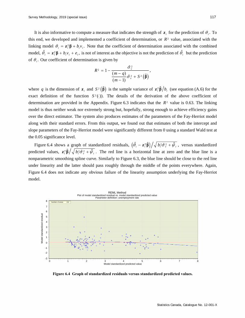
Survey Methodology, 2019 (special issue) 117
Statistics Canada, Catalogue No. 12-001-X
It is also informative to compute a measure that indicates the strength of iz for the prediction of .i To
this end, we developed and implemented a coefficient of determination, or 2R value, associated with the
linking model .Ti i i ib v z β Note that the coefficient of determination associated with the combined
model, ˆ ,Ti i i i ib v e z β is not of interest as the objective is not the prediction of i but the prediction
of .i Our coefficient of determination is given by
22
2 2
ˆ1 ,
ˆˆ1
v
v
Rm q
Sm
β
where q is the dimension of iz and 2 ˆS β is the sample variance of ˆTi ibz β (see equation (A.6) for the
exact definition of the function 2 ( )).S The details of the derivation of the above coefficient of
determination are provided in the Appendix. Figure 6.3 indicates that the 2R value is 0.63. The linking
model is thus neither weak nor extremely strong but, hopefully, strong enough to achieve efficiency gains
over the direct estimator. The system also produces estimates of the parameters of the Fay-Herriot model
along with their standard errors. From this output, we found out that estimates of both the intercept and
slope parameters of the Fay-Herriot model were significantly different from 0 using a standard Wald test at
the 0.05 significance level.
Figure 6.4 shows a graph of standardized residuals, 2 2ˆ ˆ ˆˆ ,Ti i i v ib z β versus standardized
predicted values, 2 2ˆ ˆˆ .Ti i v ib z β The red line is a horizontal line at zero and the blue line is a
nonparametric smoothing spline curve. Similarly to Figure 6.3, the blue line should be close to the red line
under linearity and the latter should pass roughly through the middle of the points everywhere. Again,
Figure 6.4 does not indicate any obvious failure of the linearity assumption underlying the Fay-Herriot
model.
Figure 6.4 Graph of standardized residuals versus standardized predicted values.
Number of areas 131
REML Method Plot of model standardized residual vs. model standardized predicted value
Parameter definition: unemployment rate
0 1 2 3 4 5 6 7 8 Model standardized predicted value
Mo
de
l sta
nda
rdiz
ed
res
idu
al
8
7
6
5
4
3
2
1
0
-1
-2
-3

118 Hidiroglou et al.: Development of a small area estimation system at Statistics Canada
Statistics Canada, Catalogue No. 12-001-X
Figure 6.5 shows a graph of squared standardized residuals versus standardized predicted values. The
red line is a horizontal line at one and the blue line is again a nonparametric smoothing spline curve. This
graph is used to check the homoscedasticity assumption; i.e., the assumption that the model variance 2v is
constant. Under homoscedasticity, the blue line should be close to the red line everywhere. The graph does
not reveal any obvious presence of heteroscedasticity.
Figure 6.5 Graph of square standardized residuals versus standardized predicted values.
Figure 6.6 shows a QQ-plot of standardized residual quantiles versus standard normal quantiles. It is
used to verify the normality assumption of the errors i ib v and .ie The graph does indicate a modest
departure from normality. However, Rao and Molina (2015, page 138) argued that EBLUP estimates and
their corresponding MSE estimates are generally robust to deviations from normality.
The system also computes Cook’s distances to identify areas that could have a significant influence on
the estimate ˆ .β The Cook distance for area i is given by
2 2
1
1 ˆ ˆ ˆ ˆ ,ˆˆ
TmT j ji ii
j j v j
Dq b
z z
β β β β
where ˆ iβ is the estimate of β obtained after deleting area .i A plot of the influences iD is provided in
Figure 6.7. One area seems to have a relatively large influence compared with other areas 1.2851 .iD
This area has the largest standardized predicted value and the second largest predicted value. Its standardized
residual is -1.88, which is not extreme, although not very small either. Its sample size is large (number of
sampled persons in the labour force close to 500) and its smooth variance estimate, ˆ ,i is relatively small
compared with other areas. All these reasons explain why this area was detected as being influential. In this
application, we decided to keep this area in the model as its influence was not large enough to make a big
difference in the SAE estimates and their corresponding MSE estimates.
Number of areas 131
REML Method Plot of square of model standardized residual vs. model standardized predicted value
Parameter definition: unemployment rate
0 1 2 3 4 5 6 7 8 Model standardized predicted value
Sq
ua
re o
f mo
de
l sta
nda
rdiz
ed
re
sid
ua
l
30
20
10
0
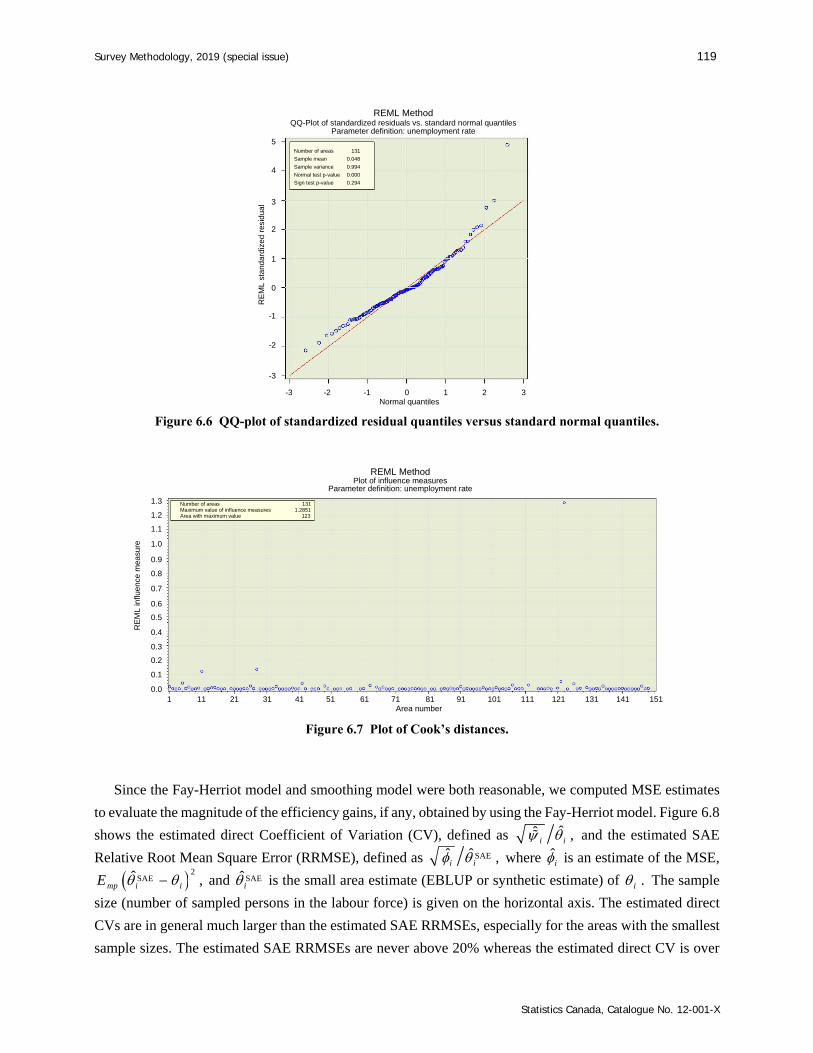
Survey Methodology, 2019 (special issue) 119
Statistics Canada, Catalogue No. 12-001-X
Figure 6.6 QQ-plot of standardized residual quantiles versus standard normal quantiles.
Figure 6.7 Plot of Cook’s distances.
Since the Fay-Herriot model and smoothing model were both reasonable, we computed MSE estimates
to evaluate the magnitude of the efficiency gains, if any, obtained by using the Fay-Herriot model. Figure 6.8
shows the estimated direct Coefficient of Variation (CV), defined as ˆˆ ,i i and the estimated SAE
Relative Root Mean Square Error (RRMSE), defined as SAEˆ ˆ ,i i where i is an estimate of the MSE,
2SAEˆ ,mp i iE and SAE
i is the small area estimate (EBLUP or synthetic estimate) of .i The sample
size (number of sampled persons in the labour force) is given on the horizontal axis. The estimated direct
CVs are in general much larger than the estimated SAE RRMSEs, especially for the areas with the smallest
sample sizes. The estimated SAE RRMSEs are never above 20% whereas the estimated direct CV is over
Number of areas 131 Maximum value of influence measures 1.2851 Area with maximum value 123
REML Method Plot of influence measures
Parameter definition: unemployment rate
1 11 21 31 41 51 61 71 81 91 101 111 121 131 141 151 Area number
RE
ML
influ
ence
mea
sure
1.3
1.2
1.1
1.0
0.9
0.8
0.7
0.6
0.5
0.4
0.3
0.2
0.1
0.0
Number of areas 131
Sample mean 0.048
Sample variance 0.994
Normal test p-value 0.000
Sign test p-value 0.294
REML Method QQ-Plot of standardized residuals vs. standard normal quantiles
Parameter definition: unemployment rate
-3 -2 -1 0 1 2 3 Normal quantiles
RE
ML
sta
nda
rdiz
ed r
esid
ua
l
5
4
3
2
1
0
-1
-2
-3

120 Hidiroglou et al.: Development of a small area estimation system at Statistics Canada
Statistics Canada, Catalogue No. 12-001-X
300% for one area. The estimated SAE RRMSEs are also very stable as a function of the sample size unlike
the erratic behavior of the estimated direct CVs. For the areas with the largest sample sizes, both estimates
are very similar, as expected. This indicates that SAE methods can lead to a substantial increase of precision
over direct estimation methods, particularly for the smallest areas.
Figure 6.8 Graph of estimated direct CVs and SAE RRMSEs as a function of sample size.
For the month of May 2016, we had the luxury of having a very reliable source for the estimation of the
unemployment rates: the 2016 long form Census administered to roughly one-fourth of the households
throughout Canada. The Census sample size is much larger than the LFS sample size in all the areas of
interest. Therefore, we used the 2016 Census direct estimates, denoted by Censusˆ ,i as a gold standard for
evaluating the accuracy of both the LFS direct estimates and SAE estimates. We computed Absolute
Relative Differences (ARD) between LFS direct estimates and Census estimates, Census Censusˆ ˆ ˆ ,i i i
as well as ARDs between SAE estimates and Census estimates, SAE Census Censusˆ ˆ ˆ .i i i These ARDs
were then averaged within 5 different homogeneous subgroups with respect to sample size. Table 6.1
summarizes the results.
Table 6.1 Average ARD of SAE estimates and LFS direct estimates expressed in percentage
Sample size Average ARD between LFS direct estimates and Census
estimates
Average ARD between SAE estimates and Census
estimates
Average ARD between HB estimates and Census
estimates 28 smallest areas 70.4% 17.7% 18.3% Next 28 smallest areas 38.7% 18.9% 19.0% Next 28 smallest areas 26.2% 13.8% 14.1% Next 28 smallest areas 20.9% 12.7% 13.0% 28 largest areas 13.2% 10.2% 10.3% Overall 33.9% 14.7% 14.9% Note: Out of the 149 areas of interest in the LFS, 9 were excluded from this table: six where the LFS number of sampled persons in the labour
force was 0 and three that were no longer in the list of CMAs /CAs after the 2016 Census.
Composite estimate (131 areas) Synthetic estimate (18 areas) Direct estimate (131 areas)
REML Method Plot of direct CV and SAE RRMSE by sample size for each area
Parameter definition: unemployment rate
0 10 24 36 48 58 80 103 128 151 202 296 542 853 1,239 Sample size
Dire
ct C
V o
r S
AE
RR
MS
E
4
3
2
1
0

Survey Methodology, 2019 (special issue) 121
Statistics Canada, Catalogue No. 12-001-X
As expected, the ARD between the LFS and Census direct estimates decreases as the sample size
increases. This may suggest that the conceptual differences between these two surveys and nonsampling
errors are reasonably small compared with the sampling error, especially for the smallest areas where the
sampling error may be the main contributor to the ARD. The SAE estimates are much closer to the Census
estimates than the LFS direct estimates, particularly for the smallest areas where improvement is most
needed. This confirms that our underlying models are reasonable in this application.
For comparison purposes, we also computed HB estimates, HBˆ ,i based on the matched Fay-Herriot
model with the noninformative priors for ,β 2v and i provided in Section 5. We then computed ARDs
between HB estimates and Census estimates, HB Census Censusˆ ˆ ˆ .i i i Results are given in the last column
of Table 6.1. The averaged ARDs of the HB estimates are close to those of the EBLUP estimates.
7 Conclusion
A frequent demand from users of data from NSOs is for more granularity for use in planning and policy
research purposes. NSOs can no longer simply increase the sample sizes of their surveys to obtain reliable
estimates at the requested level of detail. Reasons for this include the high costs of doing so, response burden
concerns, as well as the difficult task of obtaining responses from sampled units. An alternative being
investigated by many NSOs is the use of small area estimation techniques that provide a way to address the
demand for more granular data. With this in mind, Statistics Canada began the development of an SAE
production system in the early 2000s and now have such a system available to their statistical programs.
The production system handles area and unit level models, with multiple options such as different methods
to estimate the variance components, different linking models and both the EBLUP and HB estimation
methods. It is currently being used to produce experimental estimates for several Statistics Canada statistical
programs and it is expected that the first published small area estimates will be available in 2019.
As it was mentioned in the introduction, the only existing software in 2006 that would produce small
area estimates and their associated mean squared estimates was sponsored by the EURAREA (2004) project.
The current production system developed at Statistics Canada is written in SAS, with its methodology
closely following Rao (2003) and includes some recent advances. As it stands, it satisfies the existing
requirements for small area estimation at Statistics Canada. However, as the use of small area estimation
becomes more common within Statistics Canada, there will be a need to add functionality to the system to
meet this demand. The recent book authored by Rao and Molina (2015) provides an idea of how much
development has taken place in small area estimation during recent years. The incorporation of all this
development into the production system would be extremely time consuming, expensive, and may not be
directly applicable to the needs of Statistics Canada. It, therefore, follows that options other than
programming these new functionalities in the current SAS production system should be considered. One
option would be to investigate how packages developed elsewhere, such as those written in ,R can be
integrated into it. Notable packages written in R include sae (Molina and Marhuenda, 2015), mme
122 Hidiroglou et al.: Development of a small area estimation system at Statistics Canada
Statistics Canada, Catalogue No. 12-001-X
(Lopez-Vizcaino, Lombardia and Morales, 2014), saery (Esteban, Morales and Perez, 2014) and sae2 (Fay
and Diallo, 2015). These packages include small area procedures that are not in the present system such as
multinomial linear mixed models, area level models with time effects and time series area level models
supporting univariate and multivariate applications. The existing SAS production system meets the needs
of Statistics Canada at this point in time, and there are no concrete plans to add functionality to it.
Acknowledgements
We would like to thank the reviewers for their comments and suggestions that led to improvements in
this paper.
Appendix Justification of the coefficient of determination
In order to determine a coefficient of determination associated with the linking model, ,Ti i i ib v z β
we first rewrite it as
,Ti i iv z β
where i i ib and .i i ibz z We assume that an intercept is implicitly or explicitly included in ;iz
i.e., there exists a vector λ such that 1.Ti λ z In other words, we assume that there exists a vector λ such
that .Ti ib λ z If ,i 1, , ,i m were known, we could estimate the unknown vector of model
parameters β by the least squares estimator
1
*1 1
ˆm m
Ti i i i
i i
β z z z
and the unknown model variance 2v by the unbiased estimator
2
*12*
ˆˆ .
mT
i iiv m q
z β
The well-known adjusted coefficient of determination is
2*2
ideal 21
1
ˆ1 ,
1
v
m
ii
Rm
(A.1)
where 11
.m
iim
It is an ideal coefficient of determination because it cannot be computed (since i
is unknown) but this is the target we would like to estimate. Simply replacing i with i does not solve
the problem as i reflects the combined model and not just the linking model. The resulting coefficient of
Survey Methodology, 2019 (special issue) 123
Statistics Canada, Catalogue No. 12-001-X
determination would typically be too small. To obtain a better estimate of 2ideal ,R we first decompose
2
1
m
ii
as
2 22
* * * *1 1 1 1
ˆ ˆ ˆ ˆ2 .m m m m
T T T Ti i i i i i i
i i i i
z β z β z β z β (A.2)
Assuming that an intercept is implicitly or explicitly included in iz and from the expression for *ˆ ,β we
have that
*1
ˆm
Ti i i
i
z β z 0 (A.3)
and
*1
ˆ 0.m
Ti i
i
z β (A.4)
From (A.4), we can rewrite as *ˆ ,T z β where 1
1.
m
iim
z z As a result, the cross product term
in (A.2) vanishes and equation (A.2) reduces to
2 2 2
* * *1 1 1
2 2* *
ˆ ˆ ˆ
ˆˆ 1 ,
m m mT T T
i i i ii i i
vm q m S
z β z β z β
β
(A.5)
where
2
* *12*
ˆ ˆˆ .
1
mT TiiSm
z β z ββ
(A.6)
From (A.5), it follows that the ideal coefficient of determination (A.1) can be rewritten as
2*2 2
ideal * *
2 2* *
ˆ ˆ ˆ1 ( , ).ˆˆ
1
vv
v
R fm q
Sm
β
β
(A.7)
The only unknown quantities in (A.7) are *β and 2*ˆ .v A computable coefficient of determination can
thus be obtained by replacing *β and 2*ˆ v in (A.7) with β and 2ˆ ,v the consistent estimators of β and 2
v
implemented in the SAE system and described in Section 3. The resulting coefficient of determination can
be expressed as 2 2ˆ ˆ, ,vR f β with the function ,f defined in (A.7), and is a consistent estimator
of the ideal coefficient of determination 2ideal .R
References
Battese, G.E., Harter, R.M. and Fuller, W.A. (1988). An error-components model for prediction of crop areas using survey and satellite data. Journal of the American Statistical Association, 83, 28-36.
124 Hidiroglou et al.: Development of a small area estimation system at Statistics Canada
Statistics Canada, Catalogue No. 12-001-X
Beaumont, J.-F., and Bocci, C. (2016). Small area estimation in the Labour Force Survey. Paper presented at the Advisory Committee on Statistical Methods, May 2016, Statistics Canada.
Brackstone, G.J. (1987). Small area data: Policy issues and technical challenges. In Small Area Statistics, (Eds., R. Platek, J.N.K. Rao, C.-E. Särndal and M.P. Singh), New York: John Wiley & Sons, Inc., 3-20.
Chib, S., and Greenberg, E. (1995). Understanding the Metropolis-Hastings algorithm. American Statistician, 49, 327-335.
Dick, P. (1995). Modelling net undercoverage in the 1991 Canadian Census. Survey Methodology, 21, 1, 45-54. Paper available at https://www150.statcan.gc.ca/n1/en/pub/12-001-x/1995001/article/14411-eng.pdf.
Drew, D., Singh, M.P. and Choudhry, G.H. (1982). Evaluation of small area estimation techniques for the Canadian Labour Force Survey. Survey Methodology, 8, 1, 17-47. Paper available at https://www150.statcan.gc.ca/n1/en/pub/12-001-x/1982001/article/14328-eng.pdf.
Esteban, M.D., Morales, D. and Perez, A. (2014). saery: Small Area Estimation for Rao and Yu Model. URL http://CRAN.R-project.org/package=saery. R package version 1.0.
Estevao, V., Hidiroglou, M.A. and You, Y. (2015). Area Level Model, Unit Level, and Hierarchical Bayes Methodology Specifications. Internal document, Statistics Canada.
EURAREA (2004). Enhancing Small Area Estimation Techniques to meet European Needs. https://cordis.europa.eu/project/rcn/58374_en.html.
Fay, R.E., and Diallo, M. (2015). sae2: Small Area Estimation: Time-Series Models. URL http://CRAN.Rproject.org/package=sae2. R package version 0.1-1.
Fay, R.E., and Herriot, R.A. (1979). Estimation of income for small places: An application of James-Stein procedures to Census data. Journal of the American Statistical Association, 74, 269-277.
Fuller, W.A., and Rao, J.N.K. (2001). A regression composite estimator with application to the Canadian Labour Force Survey. Survey Methodology, 27, 1, 45-51. Paper available at https://www150.statcan.gc.ca/n1/en/pub/12-001-x/2001001/article/5853-eng.pdf.
Gambino, J., Kennedy, B. and Singh, M.P. (2001). Regression composite estimation for the Canadian Labour Force Survey: Evaluation and implementation. Survey Methodology, 27, 1, 65-74. Paper available at https://www150.statcan.gc.ca/n1/pub/12-001-x/2001001/article/5855-eng.pdf.
Gelfand, A.E., and Smith, A.F.M. (1990). Sample-based approaches to calculating marginal densities. Journal of the American Statistical Association, 85, 972-985.
Ghangurde, P.D., and Singh, M.P. (1977). Synthetic estimation in periodic household surveys. Survey Methodology, 3, 2, 152-181.
Gonzalez, M.E., and Hoza, C. (1978). Small-area estimation with application to unemployment and housing estimates. Journal of the American Statistical Association, 73, 7-15.

Survey Methodology, 2019 (special issue) 125
Statistics Canada, Catalogue No. 12-001-X
Kott, P. (1989). Robust small domain estimation using random effects modeling. Survey Methodology, 15, 1, 3-12. Paper available at https://www150.statcan.gc.ca/n1/pub/12-001-x/1989001/article/14581-eng.pdf.
Li, H., and Lahiri, P. (2010). Adjusted maximum method in the small area estimation problem. Journal of Multivariate Analysis, 101, 882-892.
Lopez-Vizcaino, E., Lombardia, M.J. and Morales, D. (2014). mme: Multinomial Mixed Effects Models, 2014. URL http://CRAN.R-project.org/package=mme. R package version 0.1-5.
Molina, I., and Marhuenda, Y. (2015). sae: An R package for small area estimation. The R Journal, 7, 1, 81-98.
Prasad, N.G.N., and Rao, J.N.K. (1990). The estimation of the mean squared error of small-area estimators. Journal of the American Statistical Association, 85, 163-171.
Prasad, N.G.N., and Rao, J.N.K. (1999). On robust small area estimation using a simple random effects model. Survey Methodology, 25, 1, 67-72. Paper available at https://www150.statcan.gc.ca/n1/pub/12-001-x/1999001/article/4713-eng.pdf.
Rao, J.N.K. (2003). Small Area Estimation. New York: John Wiley & Sons, Inc.
Rao, J.N.K., and Molina, I. (2015). Small Area Estimation. New York: John Wiley & Sons, Inc.
Rivest, L.-P., and Belmonte, E. (2000). A conditional mean squared error of small area estimators. Survey Methodology, 26, 1, 67-78. Paper available at https://www150.statcan.gc.ca/n1/pub/12-001-x/2000001/article/5179-eng.pdf.
Rubin-Bleuer, S. (2014). Specifications for EBLUP and Pseudo-EBLUP Estimators with Nonnegligible Sampling Fractions. Statistics Canada document.
Rubin-Bleuer, S., Jang, L. and Godbout, S. (2016). The Pseudo-EBLUP estimator for a weighted average with an application to the Canadian Survey of Employment, Payrolls and Hours. Journal of Survey Statistics and Methodology, 4, 417-435.
Singh, M.P., and Tessier, R. (1976). Some estimators for domain totals. Journal of the American Statistical Association, 71, 322-325.
Singh, A.C., Kennedy, B. and Wu, S. (2001). Regression composite estimation for the Canadian Labour Force Survey with a rotating panel design. Survey Methodology, 27, 1, 33-44. Paper available at https://www150.statcan.gc.ca/n1/en/pub/12-001-x/2001001/article/5852-eng.pdf.
Stukel, D., and Rao, J.N.K. (1997). Small-area estimation under two-fold nested error regression model. Journal of Statistical Planning and Inference, 78, 131-147.
Wang, J., and Fuller, W.A. (2003). The mean square error of small area estimators constructed with estimated area variances. Journal of American Statistical Association, 98, 716-723.
Wang, J., Fuller, W.A. and Qu, Y. (2008). Small area estimation under a restriction. Survey Methodology, 34, 1, 29-36. Paper available at https://www150.statcan.gc.ca/n1/pub/12-001-x/2008001/article/10619-eng.pdf.

126 Hidiroglou et al.: Development of a small area estimation system at Statistics Canada
Statistics Canada, Catalogue No. 12-001-X
You, Y., and Rao, J.N.K. (2002). A pseudo empirical best linear unbiased prediction approach to small area estimation using survey weights. The Canadian Journal of Statistics, 30, 431-439.
You, Y., Rao, J.N.K. and Dick, P. (2004). Benchmarking hierarchical Bayes small area estimators in the Canadian census undercoverage estimation. Statistics in Transition, 6, 631-640.
You, Y., Rao, J.N.K. and Hidiroglou, M. (2013). On the performance of self benchmarked small area estimators under the Fay-Herriot area level model. Survey Methodology, 39, 1, 217-229. Paper available at https://www150.statcan.gc.ca/n1/pub/12-001-x/2013001/article/11830-eng.pdf.

Survey Methodology, 2019 (special issue) 127 Vol. 45, No. 1, pp. 127-144 Statistics Canada, Catalogue No. 12-001-X
1. Chithran Vasudevan, Department of Mathematics and Statistics, Memorial University, St.John’s, NL A1C 5S7. E-mail: [email protected];
Asokan Mulayath Variyath, Department of Mathematics and Statistics, Memorial University, St.John’s, NL A1C 5S7. E-mail: [email protected]; Zhaozhi Fan, Department of Mathematics and Statistics, Memorial University, St.John’s, NL A1C 5S7. E-mail: [email protected].
Weighted censored quantile regression
Chithran Vasudevan, Asokan Mulayath Variyath and Zhaozhi Fan1
Abstract
In this paper, we make use of auxiliary information to improve the efficiency of the estimates of the censored quantile regression parameters. Utilizing the information available from previous studies, we computed empirical likelihood probabilities as weights and proposed weighted censored quantile regression. Theoretical properties of the proposed method are derived. Our simulation studies shown that our proposed method has advantages compared to standard censored quantile regression.
Key Words: Empirical Likelihood; Right censoring; Kaplan-Meier Estimator.
1 Introduction
In quantile regression (Koenker, 2005), the conditional quantiles of the response variable for a given set
of predictor variables are modelled. The regression parameters are estimated by minimizing a check loss
function at a specific quantile, , instead of the square loss function as in the standard linear regression. A
quantile regression model based on properly selected quantiles could provide a global assessment of the
covariate effects on the response, which is often ignored by the standard linear regression model. Recently,
censored quantile regression has been studied extensively. Powell (1984) introduced the least absolute
deviation (LAD) estimator, also called the median regression model for the left censored survival data, using
the censored Tobit model (Tobin, 1958). Powell (1986) generalized the LAD estimation to any quantile.
Portnoy (2003) introduced a censored quantile regression model under random censoring as a
generalization of the Kaplan-Meier estimator recursively using the Kaplan-Meier estimator (Kaplan and
Meier, 1958). Peng and Huang (2008) developed a censored quantile regression model based on the Nelson-
Aalen estimator using counting processes and martingale theory. In survival analysis setup, for the thi
1, 2, ,i n subject, let iT be the logarithm of the failure time, iC the logarithm of right censoring
time, iX the p -vector covariate and let min ,i i iY T C be the logarithm of the survival time. For a
given quantile, , the regression coefficients, ,β can be estimated as
1
ˆ arg min min , ,p
n
i i ii
Y C
β X βR
Τ (1.1)
where 0 ,u u u is the check loss function.
In many studies, we may have some information about the target population from previous studies. This
is common in survey sampling since surveys are carried out repeatedly with similar objectives. For example,
in survey sampling, information about the population mean and variance could be available from previous
surveys or records. The information of the parameters as well as type of relationship, distributional
128 Vasudevan, Variyath and Fan: Weighted censored quantile regression
Statistics Canada, Catalogue No. 12-001-X
assumptions, etc. also could be considered as auxiliary information available for analysis. The auxiliary
information could be effectively used to improve the efficiency of the statistical inference (Kuk and Mak,
1989; Rao, Kovar and Mantel, 1990; Chen and Qin, 1993). The idea used in this paper can be easily
extendable in survey sampling to arrive efficient parameter estimates by making use of the information
available from previous surveys.
Consider a known relationship between the survival time, Y (or the failure time, )T and a set of
covariates ,X as ; ,Y f X θ where θ is the parameter of interest. The knowledge about this
relationship can be treated as auxiliary information. In a more general case, the auxiliary information can
be expressed as ; 0E g Z θ for some d -dimensional parameter, ,dRθ where Z is the observed
data from the present study and ; ,qg RZ θ some function with .q d The parameter, θ could be
unknown, but can be estimated using the information available from previous studies.
Chen and Qin (1993) introduced the use of auxiliary information to improve the efficiency of estimators
in the context of survey sampling using empirical likelihood (Owen, 1988, 2001). Li and Wang (2003)
accommodated the auxiliary information to the censored linear regression model using empirical likelihood
by defining a synthetic variable (Koul, Susarla and Ryzin, 1981). Fang, Li, Lu and Qin (2013) proposed the
effective use of auxiliary information in the linear regression model with right censored data using empirical
likelihood, by utilizing the Buckley-James (Buckley and James, 1979) estimating equation. Tang and Leng
(2012) introduced an empirical likelihood based linear quantile regression model using auxiliary
information.
In this paper, we propose an empirical likelihood (EL) based approach to accommodate auxiliary
information to the censored quantile regression. EL is a non-parametric likelihood approach proposed by
Owen (1988, 2001), which has similar properties of parametric likelihood. We utilize the EL based data
driven probabilities as the weights by using the estimating function, ;g Z θ and incorporate those weights
into the censored quantile regression model. The resulted weighted censored quantile regression parameter
can be estimated as
1
ˆ arg min min , ,p
n
i i i ii
Y C
β X βR
Τ (1.2)
where ’si are the weights. We propose to use the EL based data driven probabilities as the weights. Our
simulation results show that the EL based weighted censored quantile regression performs more efficiently
than the standard linear censored quantile regression.
The rest of the paper is organized as follows. In Section 2, we present the estimation procedure of the
EL based data driven probabilities. In Section 3, we introduce the EL based weighted censored quantile
regression and investigate the asymptotic properties of the estimators. In Section 4, performance analysis of
the proposed method is conducted using the simulations. The application to the north central cancer
treatment lung cancer data is also presented as an illustration. Our conclusions are given in Section 5.

Survey Methodology, 2019 (special issue) 129
Statistics Canada, Catalogue No. 12-001-X
2 Estimation of weights using empirical likelihood
We develop a method that converts the auxiliary information to the EL based data driven probabilities,
which are further used in the weighted censored quantile regression as the weights. Qin and Lawless (1994)
developed the EL approach based on a set of estimating equations. Let 1
ni iZ be the observed data and the
available auxiliary information is represented by the estimating function ;ig Z θ with parameter, θ which
is known. Then, the maximum empirical likelihood is given by
EL1 1 1
sup : 0, 1, ; 0 ,n n n
i i i i ii i i
L P P P P g
θ Z θ (2.1)
where Pri i iP Z z and θ is the parameter in the auxiliary information which can be assumed to be
known. The parameter, θ could be any parametric information available from the previous studies which
has an influence on the model parameter, .β For a given ; ,ig Z θ θ should satisfy ; 0iE g Z θ
to avoid the non-existence of solutions due to convex hull issues. This is the scenario for when zero is not
an inner point of the convex hull of the ; , 1, 2, , ,ig i nZ θ which will fail to provide positive ’s.iP
For a given value of 0 ,θ θ using the Lagrange multiplier method, EL 0L θ attains its maximum at
0
0
0
1, 1, 2, , .
1 ;i
i
P i nn g
θZ θ
Τ
(2.2)
The Lagrange multiplier, 0
is the solution to the equation
0
0
1 0
;0.
1 ;
ni
i i
g
n g
Z θ
Z θΤ
The estimated ’siP are used as the weights i in (1.2) for the weighted censored quantile
regression. In some cases, θ may not be available and in such situations, we can use an estimate of ,θ say ˆ
Aθ obtained from previous studies. Chen and Qin (1993) showed that for a random sample, ,iY and ’siP
are estimated using (2.2), 1
n
n i iiF y P Y y
has smaller variance than the empirical distribution
function, 11
ˆ .n
n in iF y Y y
As a result, with Bahadur representation (Bahadur, 1966), for a given
0 1 , the quantile estimate, 1nF has smaller variance than 1ˆ
nF (See Kuk and Mak, 1989;
Rao et al., 1990). Hence our proposed method is expected to be more efficient than the ordinary censored
quantile regression.
3 Estimation of weighted censored quantile regression parameters
Define the distribution function of iT conditional on the p -vector covariate, iX as iT iF t X
Pr .i iT t X Let log 1 Pr , , 1 ,iT i i i i i it T t N t Y t X X and iM t
.ii T i iN t t Y X Here
iT i X is the cumulative hazard function conditional on ,i iN tX is
the counting process and iM t is the martingale process associated with iN t (Fleming and Harrington,
2011). We consider an extension of censored quantile regression estimation procedure proposed by Peng
and Huang (2008), incorporating the ’siP as known weights arrived based on the auxiliary information
130 Vasudevan, Variyath and Fan: Weighted censored quantile regression
Statistics Canada, Catalogue No. 12-001-X
available through the known parameter . Note that and β are distinct parameters and estimating
function :g z used for computing ’siP are different from the estimating functions used for quantile
regression parameters in (1.1). Since ’siP are independent of , i i iE P M t X 0 (by the
martingale property) for 0,t we have
0 0
1
,i i
n
i i i T i ii
E n P N e e Y
X β X βX X 0Τ Τ (3.1)
where 0 β denotes the true ,β in (1.2) for a given quantile, .
Since , 1, 2, ,iT i i n X are unknown functions, Peng and Huang (2008) derived the
relationship between 0iT i ie Y X β XΤ and 0 β to use (3.1) to estimate 0 .β Using the fact that
0i uiF e X β XF
Τ and utilizing the monotonicity of 0TiX in , they showed that
0
0,i i u
T i i ie Y Y e dH u
X β X βX Τ Τ where log 1H u u for 0 1.u
So, our weighted censored quantile regression estimating equation is
, ,nn S β 0 (3.2)
where
01
, .i i
nu
n i i i ii
S P e Y e dH u
X β X ββ X Τ Τ
Here ’siP are defined in (2.2). Let , ,ns E S β β and the martingale property of gives
0 , .s β 0 For a particular quantile, k and an estimator of 0ˆ,k k β β is a right-continuous step
function which jumps only on a grid, 0 10 1 .L L U Here L depends on the
sample size, .n The size of L is defined as 1max .L k kk
For different quantiles, 0 1 0 1, , , 0 1 ,L L based on (3.2), we can obtain
ˆ 1, 2, ,k k L β by recursively solving the following monotone estimating equation for :kβ
1ˆ
11 0
.k ri i
n k
i i i i r ri r
n P e Y e H H
X β X βX 0Τ Τ (3.3)
We define the estimators, ˆkβ as the generalized solutions (Fygenson and Ritov, 1994) because equation
(3.3) is not continuous and the solution may not be unique.
3.1 Asymptotic theory
We derived the asymptotic properties of the EL based weighted censored quantile regression estimators
using the approach of Peng and Huang (2008). Now we prove the uniform consistency and weak Gaussian
convergence of the proposed weighted censored quantile regression estimator, ˆ .β
Define Pr ,F t Y t X X Pr ,F t Y t X X Pr , 1 ,F t Y t X X f y X
f y dF y dy X X and .f y dF y dyX X (For a vector ,h 2 th, lTh hh h l
component of ,h h is the Euclidean norm of .)h

Survey Methodology, 2019 (special issue) 131
Statistics Canada, Catalogue No. 12-001-X
Define 0 0; ,i i igW Z θ XΤ 1, 2, ,i n as a p -vector.
Regularity conditions:
R.1: The observations, , 1, 2, ,i i nZ are iid observations from some distribution. Without
loss of generality, we assume that , ,i i i iY X ZΤΤ for all 1, 2, , .i n
R.2: There exists 0θ such that 0; 0,iE g Z θ the matrix 0 0 0; ;i iE g gΣ θ Z θ Z θ Τ
is positive definite, ;gz θθ is continuous in the neighborhood of 0 .θ The matrix ;gE
Z θθ
is of full rank.
R.3: There exist functions ljH z such that for θ in the neighborhood of 0 ,θ ; ,l
j
gljH
z θ z
where for a constant 2, ljC E H C Z for 1, ,l q and 1, , .j d
R.4: sup ii
X and sup .i ii
X Y
R.5: (a) Each component of 0E e X βX Τ is a Lipschitz function of .
(b) f t x and f t x are bounded above uniformly in t and .x
R.6: (a) 0f e X b X Τ for all 0( ),db B where
00,: inf
U
pd d
b μ b μ βB R
for 0,d and ,E e X bμ b X Τ is a neighbourhood containing
0 , 0, .U β
(b) To have the positive definiteness, 2 0.E X
(c) Each component of 12 2E f e e E f e e
X b X b X b X bX X X XΤ Τ Τ Τ is
uniformly bounded in 0 0; .d db B B
R.7: For any ,
0, , infU
U vv
eigmin 0 02 0,E f e e X β X βX X Τ Τ where eigmin
denotes the minimum eigenvalue of a matrix.
Theorem 1. Assuming that the regularity conditions R.1-R.7 hold, if lim 0,Ln then
0
,
ˆsup 0,U
pv
β β where 0 .Uv
Theorem 2. Assuming that the regularity conditions R.1-R.7 hold, if 1 2lim 0,Lnn
then
1 20
ˆn β β weakly converges to a zero-mean Gaussian process for , ,Uv where
0 .Uv
To prove Theorems 1 and 2, we need to show that 0 01
max ; 1 .i pi ng o
Z θΤ We consider two
different types of ; .ig Z θ First, ;ig Z θ does not contain the censored observations, as given in (4.1).
The second, ; ,ig Z θ contains the censored observations, as given in (4.5).
In the case of uncensored observations, by Owen (1991) and Lemma 11.2 of Owen (2001), we have
01max ; .i pi n
g o n
Z θ By Lemma 1 of Tang and Leng (2012), we have under the regularity
conditions R.2, R.3; the 0
in (2.2) satisfies 0
1 .p nO So,
0 01
1max ; 1 .i p p pi n
g O o n on
Z θΤ (3.4)

132 Vasudevan, Variyath and Fan: Weighted censored quantile regression
Statistics Canada, Catalogue No. 12-001-X
Under the condition R.4; Qin and Jing (2001) proved 0 01
max ; 1i pi ng o
Z θΤ for the g with
censored observations.
Now following Owen (2001), using Taylor’s series expansion of the weights, ’siP defined in (2.2) can
be rewritten as,
0
0
0
0
0
0
0
1
1 ;
11 ; 1 1
1 11 ; ; 1, 2, , .
i
i
i p
i p
Pn g
g on
g o i nn n
θZ θ
Z θ
Z θ
Τ
Τ
Τ
Now we rewrite the ,nS β as
0
0
0 01
01
0 01
01
1 1, 1 ;
1
1 1;
1
1
i i
i i
i i
i i
nu
n i i i i pi
nu
i i ii
nu
i i i i pi
nu
i i ii
i i
S g e Y e dH u on n
e Y e dH un
g e Y e dH u on n
e Y e dH un
n
X β X β
X β X β
X β X β
X β X β
β Z θ X
X
Z θ X
X
W
Τ Τ
Τ Τ
Τ Τ
Τ Τ
Τ
Τ
01
1.i i
nu
i pi
e Y e dH u on
X β X βΤ Τ
Asymptotically, by (3.4) we have 1 ; 1, 2, , .i po i n W So,
01
1 1, .i i
nu
n i i i pi
S e Y e dH u on n
X β X ββ X Τ Τ
Asymptotically this estimating function, ,nS β is equivalent to that in Peng and Huang (2008).
Following the similar arguments of Peng and Huang (2008), we complete the proofs of Theorems 1 and 2.
As indicated in Peng and Huang (2008), the estimation of asymptotic variance of the quantile regression
estimates is not easy since the covariance matrix of the limiting process of 0ˆn involves
unknown density function f y X and .f y X Instead of using a smoothing or other numerical
approximations, we suggest a simple bootstrap approach to estimate the standard errors of the regression
estimates. This approach is used in our performance analysis discussed in next section.
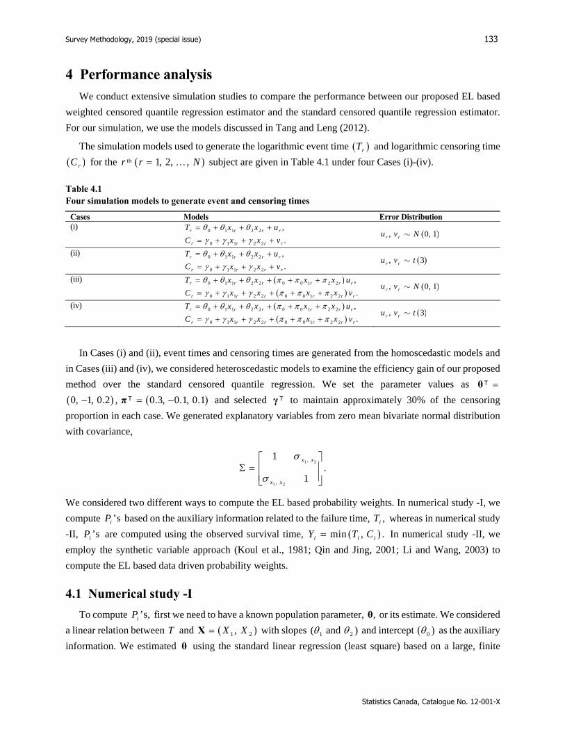
Survey Methodology, 2019 (special issue) 133
Statistics Canada, Catalogue No. 12-001-X
4 Performance analysis
We conduct extensive simulation studies to compare the performance between our proposed EL based
weighted censored quantile regression estimator and the standard censored quantile regression estimator.
For our simulation, we use the models discussed in Tang and Leng (2012).
The simulation models used to generate the logarithmic event time rT and logarithmic censoring time
rC for the thr 1, 2, ,r N subject are given in Table 4.1 under four Cases (i)-(iv).
Table 4.1 Four simulation models to generate event and censoring times
Cases Models Error Distribution (i)
0 1 1 2 2 ,r r r rT x x u
0 1 1 2 2 .r r r rC x x v , 0, 1r ru v N~
(ii) 0 1 1 2 2 ,r r r rT x x u
0 1 1 2 2 .r r r rC x x v , 3r ru v t~
(iii) 0 1 1 2 2 0 0 1 2 2 ,r r r r r rT x x x x u
0 1 1 2 2 0 0 1 2 2 .r r r r r rC x x x x v , 0, 1r ru v N~
(iv) 0 1 1 2 2 0 0 1 2 2 ,r r r r r rT x x x x u
0 1 1 2 2 0 0 1 2 2 .r r r r r rC x x x x v , 3r ru v t~
In Cases (i) and (ii), event times and censoring times are generated from the homoscedastic models and
in Cases (iii) and (iv), we considered heteroscedastic models to examine the efficiency gain of our proposed
method over the standard censored quantile regression. We set the parameter values as θ Τ
0, 1, 0.2 , 0.3, 0.1, 0.1 π Τ and selected γ Τ to maintain approximately 30% of the censoring
proportion in each case. We generated explanatory variables from zero mean bivariate normal distribution
with covariance,
1 2
1 2
,
,
1.
1
x x
x x
We considered two different ways to compute the EL based probability weights. In numerical study -I, we
compute ’siP based on the auxiliary information related to the failure time, ,iT whereas in numerical study
-II, ’siP are computed using the observed survival time, min , .i i iY T C In numerical study -II, we
employ the synthetic variable approach (Koul et al., 1981; Qin and Jing, 2001; Li and Wang, 2003) to
compute the EL based data driven probability weights.
4.1 Numerical study -I
To compute ’s,iP first we need to have a known population parameter, ,θ or its estimate. We considered
a linear relation between T and 1 2,X XX with slopes 1( and 2 ) and intercept 0 as the auxiliary
information. We estimated θ using the standard linear regression (least square) based on a large, finite

134 Vasudevan, Variyath and Fan: Weighted censored quantile regression
Statistics Canada, Catalogue No. 12-001-X
population with size, N 10,000. We need to generate censoring times as well to compute the event
indicator, i i iT C and survival time, min ,i i iY T C to estimate the censored quantile
regression parameters. To fit the weighted censored quantile regression model given in (1.2), we generated
another n observations 1, ni i iy x with ,n N using the same models given in Table 4.1. We considered
the sample sizes, n 100 and 200 and three quantiles, 0.25, 0.50, 0.75. For our proposed method, we
estimated ’siP using the estimating function, , ;i ig t x θ defined based on the normal equations of the
linear least squares method as,
ˆ; , ; , 1, 2, , .i i i i i i ig g t t i n z θ x θ x x θ Τ (4.1)
For a given quantile, , the true value of the censored quantile regression parameters 0 β are estimated
from the population of size, N 10,000. In general, under a linear model assumption, the true value of the
censored quantile regression slope parameters are the same as the θ (i.e., 1 1 2 2, ). But
for the intercept, it is 10 0 ,F where F is the error distribution. We conducted 1,000
simulations and computed mean bias, standard error (SE) and 95% coverage probability (CP) of the model
parameter estimates for different sample sizes using 250 bootstrap samples. We compared the performance
of our proposed method (CQR-EL1) with the standard censored quantile regression (CQR) model. We
present the simulation results in Tables 4.2 to 4.5 respectively for Cases (i)-(iv) with 1 2, 0.x x
Table 4.2 Bias, SE and CP of regression parameters for Case (i) model with independent covariates
1 2, 0x x
n
CQR CQR-EL1
0.25 0.50 0.75 0.25 0.50 0.75
Bias 100 0 0.0042 0.0170 0.0647 0.0027 0.0180 0.0771
1 0.0029 0.0035 0.0094 -0.0014 -0.0048 0.0030
2 -0.0049 -0.0141 -0.0100 -0.0047 -0.0124 -0.0171
200 0 0.0218 0.0298 0.0501 0.0199 0.0322 0.0635
1 0.0016 0.0026 0.0057 0.0008 0.0028 0.0048
2 -0.0020 -0.0032 -0.0078 -0.0010 0.0001 -0.0071
SE 100 0 0.1449 0.1404 0.2268 0.1103 0.1086 0.2110
1 0.1533 0.1515 0.2141 0.1159 0.1109 0.2000
2 0.1519 0.1525 0.2198 0.1149 0.1109 0.2082
200 0 0.0973 0.0929 0.1292 0.0720 0.0703 0.1221
1 0.1040 0.1029 0.1341 0.0746 0.0718 0.1173
2 0.1041 0.1027 0.1354 0.0752 0.0717 0.1177
CP 100 0 93.3 93.4 95.7 95.8 96.6 97.0
1 94.7 95.8 96.5 95.1 96.2 97.9
2 96.0 96.3 96.4 96.4 96.4 96.9
200 0 92.3 91.9 92.7 92.7 92.5 94.8
1 94.5 96.2 95.0 95.0 95.5 96.9
2 93.6 95.0 95.2 94.2 94.9 95.8

Survey Methodology, 2019 (special issue) 135
Statistics Canada, Catalogue No. 12-001-X
Table 4.3 Bias, SE and CP of regression parameters for Case (ii) model with independent covariates
1 2, 0x x
n
CQR CQR-EL1
0.25 0.50 0.75 0.25 0.50 0.75
Bias 100 0 0.0105 0.0288 0.1088 0.0119 0.0270 0.1062
1 0.0063 0.0214 0.0169 0.0005 0.0102 0.0066
2 0.0164 0.0096 -0.0170 0.0152 0.0079 -0.0184
200 0 0.0267 0.0355 0.0821 0.0276 0.0340 0.0760
1 0.0006 -0.0032 0.0050 0.0042 0.0032 0.0024
2 0.0112 0.0025 0.0051 0.0029 -0.0038 -0.0057
SE 100 0 0.1871 0.1538 0.2980 0.1522 0.1304 0.2914
1 0.1946 0.1664 0.2698 0.1555 0.1318 0.2480
2 0.1955 0.1676 0.2733 0.1556 0.1327 0.2543
200 0 0.1235 0.1029 0.1621 0.0998 0.0871 0.1556
1 0.1301 0.1146 0.1663 0.1010 0.0893 0.1473
2 0.1315 0.1149 0.1671 0.1023 0.0897 0.1465
CP 100 0 95.5 93.1 94.7 96.2 94.8 97.2
1 95.6 93.5 96.4 95.7 95.6 97.8
2 95.9 95.4 96.4 96.0 95.0 97.2
200 0 93.1 91.2 94.0 93.0 93.8 95.7
1 95.0 95.5 95.4 94.8 95.5 96.2
2 95.5 95.7 95.5 95.0 95.2 96.3
Table 4.4 Bias, SE and CP of regression parameters for Case (iii) model with independent covariates
1 2, 0x x
n
CQR CQR-EL1
0.25 0.50 0.75 0.25 0.50 0.75
Bias 100 0 0.0062 0.0088 0.0224 0.0055 0.0085 0.0254
1 0.0042 0.0051 0.0076 0.0034 0.0016 0.0057
2 -0.0038 -0.0039 -0.0069 -0.0013 0.0003 -0.0010
200 0 0.0064 0.0072 0.0167 0.0064 0.0089 0.0195
1 0.0012 0.0038 0.0033 -0.0006 -0.0003 -0.0014
2 -0.0015 -0.0031 -0.0017 -0.0004 0.0002 0.0023
SE 100 0 0.0472 0.0466 0.0767 0.0349 0.0338 0.0737
1 0.0566 0.0570 0.0796 0.0424 0.0411 0.0708
2 0.0567 0.0575 0.0807 0.0425 0.0418 0.0720
200 0 0.0313 0.0301 0.0402 0.0225 0.0213 0.0345
1 0.0371 0.0377 0.0489 0.0276 0.0267 0.0402
2 0.0367 0.0376 0.0488 0.0270 0.0267 0.0401
CP 100 0 94.4 95.0 96.1 94.3 96.0 97.1
1 95.0 95.2 95.5 95.2 95.3 97.4
2 96.6 96.7 97.3 95.4 96.6 98.0
200 0 94.1 93.4 94.9 93.2 94.0 94.1
1 94.0 94.9 96.0 93.0 95.1 95.9
2 94.6 95.0 95.3 94.4 95.3 94.8
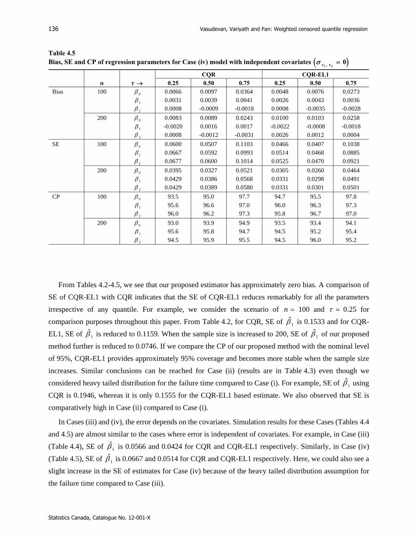
136 Vasudevan, Variyath and Fan: Weighted censored quantile regression
Statistics Canada, Catalogue No. 12-001-X
Table 4.5 Bias, SE and CP of regression parameters for Case (iv) model with independent covariates
1 2, 0x x
n
CQR CQR-EL1
0.25 0.50 0.75 0.25 0.50 0.75
Bias 100 0 0.0066 0.0097 0.0364 0.0048 0.0076 0.0273
1 0.0031 0.0039 0.0041 0.0026 0.0043 0.0036
2 0.0008 -0.0009 -0.0018 0.0008 -0.0035 -0.0028
200 0 0.0083 0.0089 0.0243 0.0100 0.0103 0.0258
1 -0.0020 0.0016 0.0017 -0.0022 -0.0008 -0.0018
2 0.0008 -0.0012 -0.0031 0.0026 0.0012 0.0004
SE 100 0 0.0600 0.0507 0.1103 0.0466 0.0407 0.1038
1 0.0667 0.0592 0.0993 0.0514 0.0468 0.0885
2 0.0677 0.0600 0.1014 0.0525 0.0470 0.0921
200 0 0.0395 0.0327 0.0521 0.0305 0.0260 0.0464
1 0.0429 0.0386 0.0568 0.0331 0.0298 0.0491
2 0.0429 0.0389 0.0580 0.0331 0.0301 0.0501
CP 100 0 93.5 95.0 97.7 94.7 95.5 97.8
1 95.6 96.6 97.0 96.0 96.3 97.3
2 96.0 96.2 97.3 95.8 96.7 97.0
200 0 93.0 93.9 94.9 93.5 93.4 94.1
1 95.6 95.8 94.7 94.5 95.2 95.4
2 94.5 95.9 95.5 94.5 96.0 95.2
From Tables 4.2-4.5, we see that our proposed estimator has approximately zero bias. A comparison of
SE of CQR-EL1 with CQR indicates that the SE of CQR-EL1 reduces remarkably for all the parameters
irrespective of any quantile. For example, we consider the scenario of n 100 and 0.25 for
comparison purposes throughout this paper. From Table 4.2, for CQR, SE of 1 is 0.1533 and for CQR-
EL1, SE of 1 is reduced to 0.1159. When the sample size is increased to 200, SE of 1 of our proposed
method further is reduced to 0.0746. If we compare the CP of our proposed method with the nominal level
of 95%, CQR-EL1 provides approximately 95% coverage and becomes more stable when the sample size
increases. Similar conclusions can be reached for Case (ii) (results are in Table 4.3) even though we
considered heavy tailed distribution for the failure time compared to Case (i). For example, SE of 1 using
CQR is 0.1946, whereas it is only 0.1555 for the CQR-EL1 based estimate. We also observed that SE is
comparatively high in Case (ii) compared to Case (i).
In Cases (iii) and (iv), the error depends on the covariates. Simulation results for these Cases (Tables 4.4
and 4.5) are almost similar to the cases where error is independent of covariates. For example, in Case (iii)
(Table 4.4), SE of 1 is 0.0566 and 0.0424 for CQR and CQR-EL1 respectively. Similarly, in Case (iv)
(Table 4.5), SE of 1 is 0.0667 and 0.0514 for CQR and CQR-EL1 respectively. Here, we could also see a
slight increase in the SE of estimates for Case (iv) because of the heavy tailed distribution assumption for
the failure time compared to Case (iii).
Survey Methodology, 2019 (special issue) 137
Statistics Canada, Catalogue No. 12-001-X
4.2 Numerical study -II
In most of the survival data with random right censoring, the observed data are the triplet
min , , , .Y T C X We consider a linear relationship between the survival time Y and the
covariates as the auxiliary information. Here we cannot use the EL estimating function, g defined in
(4.1) because of the censoring. There are other methods available in the literature which take care of the
right censoring in the linear regression.
Koul et al. (1981) introduced a synthetic data approach by transforming the survival time, rY to a
synthetic variable, rY as
; 1, 2, , ,1
r rr
r
YY r N
G Y
(4.2)
where r is the censoring indicator and G is the distribution of the censoring time. E Y E YX X
if C is independent of both X and .Y When G is unknown, we can replace it with its Kaplan-Meier
estimator. The estimator of G using the Kaplan-Meier (Kaplan and Meier, 1958) estimator is
, 0
1
ˆ1 ,1
r rY tN
Nr
N rG t
N r
(4.3)
where ’srY are ordered and the corresponding censoring indicator is .r We can estimate θ as
1 .rYθ X X X Τ Τ (4.4)
Qin and Jing (2001) and Li and Wang (2003) independently provided the estimating function to compute
the EL based data driven probabilities as
; , , ; , 1, 2, , .i i i i i i i ig g y y i n z θ x θ x x θ Τ (4.5)
We can compute the iy and ˆnG t using the sample analogues of (4.2) and (4.3) respectively.
To compute ’s,iP we consider a linear relation between Y and 1 2,X XX with slopes 1( and 2 )
and intercept 0 . We estimate θ using (4.4) based on a large, finite population with size, N 10,000.
To fit the weighted censored quantile regression model given in (1.2), we generate another n observations
1, ni i iy x with n N using the same models given in Table 4.1. For our proposed method, we estimate
’siP using the estimating function, , , ;i i ig y x θ given in (4.5).
Similar to numerical study -I, we present the results based on 1,000 simulations and report the bias,
standard error (SE) and empirical coverage probability (CP) for the nominal level of 95% based on 250
bootstrap samples. We provide the summary of the simulation results for this study in Tables 4.6-4.9.
Similar to the population information related to T (numerical study -I), conclusions are almost similar
for uncorrelated covariates. From Tables 4.6-4.9 we see that our proposed method (CQR-EL2) provides
unbiased estimates irrespective of any sample size and quantile. If we consider the coverage probability,

138 Vasudevan, Variyath and Fan: Weighted censored quantile regression
Statistics Canada, Catalogue No. 12-001-X
both CQR and CQR-EL2 provide approximately 95% coverage. For any quantile, there is a reduction in the
standard error of CQR-EL2 parameter estimates compared to CQR parameter estimates. If we consider Case
(i) as a basic model, CQR-EL2 with Case (ii) has reasonably higher SE along with CQR because of the
heavy tailed distribution of the observed survival time. When the error depended on the covariates (Cases
(iii) & (iv)), the SE of CQR-EL2 reduced considerably.
We also conducted large number of simulations with correlated covariates with 1 2,x x 0.5 as well as
constructed weights based on simple relationship with one covariate only for both numerical studies. The
results of these simulations are not provided here to save the space. The conclusions arrived are almost
similar to the uncorrelated covariate cases.
In numerical study -I, we noticed that there is a slight reduction in SE of 2 using heteroscedastic models
for CQR-EL1. But use of the estimating function, 1, , ;i i ig y x θ (CQR-EL2), does not reduce the SE of
2 under heteroscedastic models. Since we utilized only partial population information in relation to 1 ,X
the standard error of 0 and 1 reduced for CQR-EL2 compared to CQR. The standard error of 2 was
not changed.
Our simulation studies reveal that auxiliary information greatly enhances the efficiency of estimation, if
the population information related to both 1X and 2X is available. If the population information is only
related to 1 ,X the efficiency gain is limited to 0 and 1 only. However, under heteroscedastic models,
the efficiency of estimating 2 slightly improved in numerical study -I, but not in numerical study -II.
Table 4.6 Bias, SE and CP of regression parameters for Case (i) model with independent covariates
1 2, 0x x
n
CQR CQR-EL2
0.25 0.50 0.75 0.25 0.50 0.75
Bias 100 0 0.0042 0.0170 0.0647 0.0217 0.0275 0.0720
1 0.0029 0.0035 0.0094 -0.0491 -0.0411 -0.0090
2 -0.0049 -0.0141 -0.0100 0.0116 -0.0029 -0.0194
200 0 0.0218 0.0298 0.0501 0.0220 0.0323 0.0562
1 0.0016 0.0026 0.0057 -0.0295 -0.0273 -0.0119
2 -0.0020 -0.0032 -0.0078 0.0034 0.0053 -0.0011
SE 100 0 0.1449 0.1404 0.2268 0.1273 0.1233 0.2160
1 0.1533 0.1515 0.2141 0.1475 0.1416 0.2075
2 0.1519 0.1525 0.2198 0.1416 0.1414 0.2162
200 0 0.0973 0.0929 0.1292 0.0840 0.0798 0.1239
1 0.1040 0.1029 0.1341 0.0970 0.0921 0.1278
2 0.1041 0.1027 0.1354 0.0957 0.0936 0.1304
CP 100 0 93.3 93.4 95.7 94.3 96.1 96.8
1 94.7 95.8 96.5 94.6 96.1 96.9
2 96.0 96.3 96.4 95.4 95.4 97.4
200 0 92.3 91.9 92.7 92.9 92.3 94.3
1 94.5 96.2 95.0 95.3 95.3 94.8
2 93.6 95.0 95.2 93.5 94.9 95.9
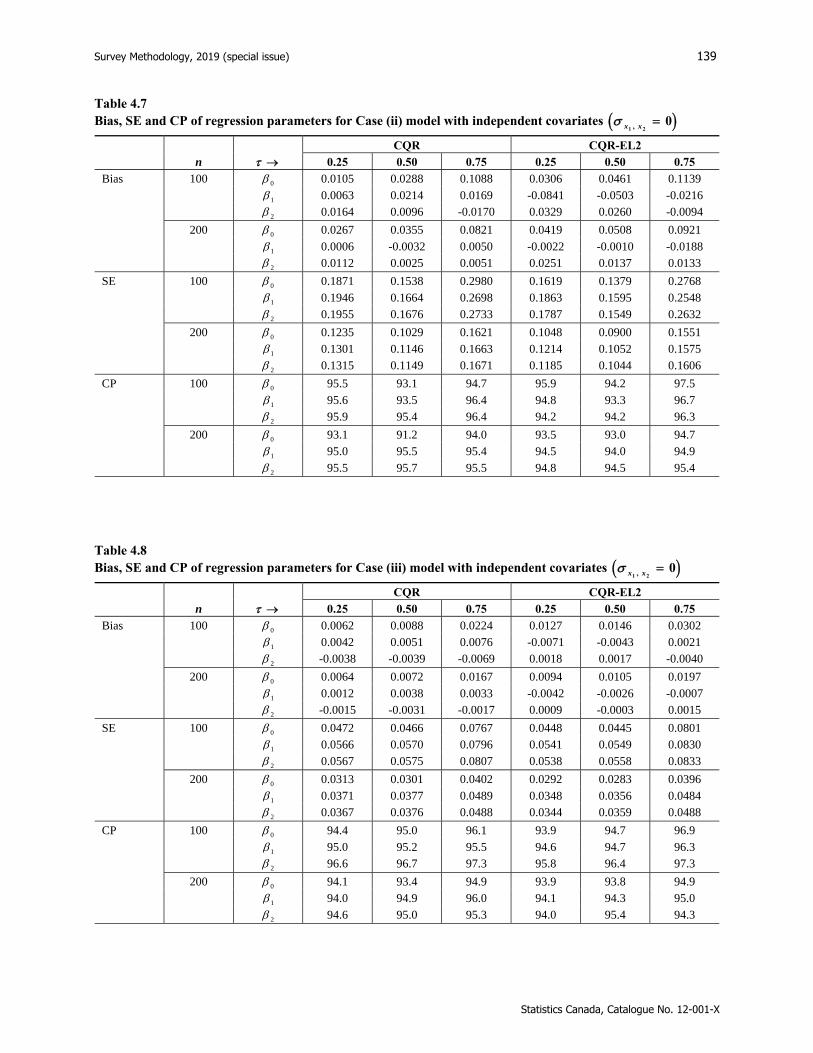
Survey Methodology, 2019 (special issue) 139
Statistics Canada, Catalogue No. 12-001-X
Table 4.7 Bias, SE and CP of regression parameters for Case (ii) model with independent covariates
1 2, 0x x
n
CQR CQR-EL2
0.25 0.50 0.75 0.25 0.50 0.75
Bias 100 0 0.0105 0.0288 0.1088 0.0306 0.0461 0.1139
1 0.0063 0.0214 0.0169 -0.0841 -0.0503 -0.0216
2 0.0164 0.0096 -0.0170 0.0329 0.0260 -0.0094
200 0 0.0267 0.0355 0.0821 0.0419 0.0508 0.0921
1 0.0006 -0.0032 0.0050 -0.0022 -0.0010 -0.0188
2 0.0112 0.0025 0.0051 0.0251 0.0137 0.0133
SE 100 0 0.1871 0.1538 0.2980 0.1619 0.1379 0.2768
1 0.1946 0.1664 0.2698 0.1863 0.1595 0.2548
2 0.1955 0.1676 0.2733 0.1787 0.1549 0.2632
200 0 0.1235 0.1029 0.1621 0.1048 0.0900 0.1551
1 0.1301 0.1146 0.1663 0.1214 0.1052 0.1575
2 0.1315 0.1149 0.1671 0.1185 0.1044 0.1606
CP 100 0 95.5 93.1 94.7 95.9 94.2 97.5
1 95.6 93.5 96.4 94.8 93.3 96.7
2 95.9 95.4 96.4 94.2 94.2 96.3
200 0 93.1 91.2 94.0 93.5 93.0 94.7
1 95.0 95.5 95.4 94.5 94.0 94.9
2 95.5 95.7 95.5 94.8 94.5 95.4
Table 4.8 Bias, SE and CP of regression parameters for Case (iii) model with independent covariates
1 2, 0x x
n
CQR CQR-EL2
0.25 0.50 0.75 0.25 0.50 0.75
Bias 100 0 0.0062 0.0088 0.0224 0.0127 0.0146 0.0302
1 0.0042 0.0051 0.0076 -0.0071 -0.0043 0.0021
2 -0.0038 -0.0039 -0.0069 0.0018 0.0017 -0.0040
200 0 0.0064 0.0072 0.0167 0.0094 0.0105 0.0197
1 0.0012 0.0038 0.0033 -0.0042 -0.0026 -0.0007
2 -0.0015 -0.0031 -0.0017 0.0009 -0.0003 0.0015
SE 100 0 0.0472 0.0466 0.0767 0.0448 0.0445 0.0801
1 0.0566 0.0570 0.0796 0.0541 0.0549 0.0830
2 0.0567 0.0575 0.0807 0.0538 0.0558 0.0833
200 0 0.0313 0.0301 0.0402 0.0292 0.0283 0.0396
1 0.0371 0.0377 0.0489 0.0348 0.0356 0.0484
2 0.0367 0.0376 0.0488 0.0344 0.0359 0.0488
CP 100 0 94.4 95.0 96.1 93.9 94.7 96.9
1 95.0 95.2 95.5 94.6 94.7 96.3
2 96.6 96.7 97.3 95.8 96.4 97.3
200 0 94.1 93.4 94.9 93.9 93.8 94.9
1 94.0 94.9 96.0 94.1 94.3 95.0
2 94.6 95.0 95.3 94.0 95.4 94.3

140 Vasudevan, Variyath and Fan: Weighted censored quantile regression
Statistics Canada, Catalogue No. 12-001-X
Table 4.9 Bias, SE and CP of regression parameters for Case (iv) model with independent covariates
1 2, 0x x
n
CQR CQR-EL2
0.25 0.50 0.75 0.25 0.50 0.75
Bias 100 0 0.0066 0.0097 0.0364 0.0189 0.0169 0.0419
1 0.0031 0.0039 0.0041 -0.0138 -0.0073 -0.0000
2 0.0008 -0.0009 -0.0018 0.0074 0.0060 0.0024
200 0 0.0083 0.0089 0.0243 0.0124 0.0119 0.0273
1 -0.0020 0.0016 0.0017 -0.0097 -0.0051 -0.0032
2 0.0008 -0.0012 -0.0031 0.0019 0.0004 -0.0020
SE 100 0 0.0600 0.0507 0.1103 0.0548 0.0486 0.1159
1 0.0667 0.0592 0.0993 0.0618 0.0581 0.1018
2 0.0677 0.0600 0.1014 0.0616 0.0578 0.1066
200 0 0.0395 0.0327 0.0521 0.0359 0.0304 0.0516
1 0.0429 0.0386 0.0568 0.0397 0.0364 0.0558
2 0.0429 0.0389 0.0580 0.0397 0.0368 0.0579
CP 100 0 93.5 95.0 97.7 92.9 95.2 97.6
1 95.6 96.6 97.0 94.2 95.5 97.4
2 96.0 96.2 97.3 96.3 97.0 97.6
200 0 93.0 93.9 94.9 93.3 94.2 95.8
1 95.6 95.8 94.7 94.0 95.5 95.2
2 94.5 95.9 95.5 94.9 96.0 94.7
Note that the value of the auxiliary parameter value plays a big role in the efficiency of the weighted
censored quantile regression parameter estimates. If the estimate of based present study data and previous
study (or known value) are very close, then all weights will be close to 1 n and solutions to (1.1) and
(1.2) remain the same. If data on previous studies are not available, we can make of the data available in the
present study to estimate the value of . In this case, if dimensions of and estimating equation ,g z
are same, then all weights will be equal to 1 n and solutions to (1.1) and (1.2) remain same. However, if
the dimensions of ,g z is greater than that of , the weights ˆp is no longer equal to 1 n and this
scheme provides an efficiency gain over the conventional QR estimates (Tang and Leng, 2012).
4.3 Case example
The North Central Cancer Treatment Group (NCCTG) was initiated by a group of physicians from the
north central region of the United States of America and the Mayo Clinic in Rochester, Minnesota. This
study was conducted by NCCTG to determine whether the conclusions from the patient-completed
questionnaire and those already obtained by the patient’s physician were independent or not (Loprinzi,
Laurie, Wieand, Krook, Novotny, Kugler, Bartel, Law, Bateman and Klatt, 1994). They used the
performance scores (ECOG and Karnofsky) to assess the patient’s daily activities. The dataset is available
in the “survival” package of R software with readings of 228 patients. Because of the incompleteness of
some of the variables, we had to limit the dataset to 167 observations. For the illustration of our proposed
method, we changed our focus to identify the effect of following covariates over the observed survival time
at different quantiles. We considered “age”, patient’s age in years; “sex”, (Male = 1 Female = 2); “ph.ecog”,

Survey Methodology, 2019 (special issue) 141
Statistics Canada, Catalogue No. 12-001-X
ECOG performance score measured by physician (0 = good 5 = dead); “meal.cal”, calories consumed at
meals and “wt.loss”, weight loss in the last six months as the covariates. After removing the incomplete
patient readings, the available ECOG scores were 0,1 and 2 only. We defined two dummy categorical
variables for “ph.ecog” as follows.
1, if ph.ecog 1ecog1
0, otherwise
1, if ph.ecog 2ecog2
0, otherwise.
To demonstrate the usefulness of our proposed method, we randomly selected a part (100 observations)
of the complete data (167 observations) by considering it to be the data available from the previous study.
We assumed that there exists a linear relation between the logarithm of the observed survival time and all
the continuous explanatory variables (age, meal.cal and wt.loss) as the available auxiliary information. We
estimated the 0 age meal wt, , , θ by the least square method based on 100 observations where the
response is the synthetic variable defined by (4.2). Then we computed the EL based data driven probability
weights for the present study data points (67 observations). After computing the weights, we estimated the
weighted censored quantile regression parameters using Peng and Huang (2008) method with all the
covariates. For the present study data, the censoring proportion is 0.283. Interestingly, we estimated the
regression parameters using CQR up to the th86 quantile, where as we could estimate to the th90 quantile
using CQR-EL2. Along with the estimates for the quantiles, 0.25, 0.50, 0.75, we report standard error
(SE) and 95% confidence limits using 250 bootstrap samples as well in Table 4.10.
Table 4.10 Estimates, SE and 95% CI for regression parameters of NCCTG lung cancer data
CQR CQR-EL2
0.25 0.50 0.75 0.25 0.50 0.75
Intercept 5.4777 4.2651 5.5380 4.7531 4.1729 6.4258 Age -0.0168 0.0179 0.0040 -0.0047 0.0202 -0.0032 Sex 0.7201 0.6180 0.4181 0.7606 0.6638 0.3651
ECOG1 -0.7059 -0.5449 -0.2029 -0.5701 -0.5355 -0.2884 ECOG2 -0.8677 -0.9402 -0.8336 -1.1584 -1.0612 -1.0192 MealCal 0.0004 0.0001 0.0001 0.0004 0.0001 -0.0000 WtLoss -0.0007 -0.0084 -0.0023 -0.0023 -0.0100 -0.0135
SE Intercept 1.9235 1.4314 1.7494 1.6628 1.4149 1.4666 Age 0.0277 0.0188 0.0225 0.0256 0.0184 0.0176 Sex 0.5610 0.3389 0.3716 0.5374 0.3317 0.2809
ECOG1 0.6521 0.3436 0.3375 0.6498 0.3493 0.2434 ECOG2 1.0317 0.5410 0.6061 0.9336 0.5413 0.3879 MealCal 0.0009 0.0006 0.0008 0.0009 0.0006 0.0005 WtLoss 0.0181 0.0128 0.0231 0.0157 0.0124 0.0100
CI Intercept (1.6, 9.14) (2.38, 8) (2.08, 8.94) (1.79, 8.31) (2.32, 7.87) (3.14, 8.89) Age (-0.07, 0.04) (-0.04, 0.04) (-0.04, 0.05) (-0.06, 0.04) (-0.03, 0.04) (-0.03, 0.04) Sex (-0.45, 1.74) (0, 1.33) (-0.13, 1.33) (-0.39, 1.71) (-0.04, 1.27) (-0.07, 1.03)
ECOG1 (-1.75, 0.81) (-1.15, 0.2) (-0.97, 0.35) (-1.86, 0.69) (-1.18, 0.19) (-0.78, 0.18) ECOG2 (-2.88, 1.16) (-2, 0.12) (-2.11, 0.26) (-2.83, 0.83) (-2.13, -0.01) (-1.73, -0.21) WtLoss (-0.04, 0.03) (-0.03, 0.02) (-0.05, 0.04) (-0.04, 0.02) (-0.03, 0.01) (-0.04, 0)

142 Vasudevan, Variyath and Fan: Weighted censored quantile regression
Statistics Canada, Catalogue No. 12-001-X
From Table 4.10, we see that the standard error of the estimates of all the continuous variable parameters
and the intercept reduced considerably because we considered the auxiliary information related to them. For
the remaining variables, a reduction of standard error can also be seen, even though we did not consider any
auxiliary information related to them. In the censored quantile regression with the EL based data driven
probability weights, we see narrower 95% confidence limits for all the variables compared to those using
the standard censored quantile regression.
5 Conclusions
We proposed a method which effectively use the auxiliary information to improve the efficiency of the
censored quantile regression estimator. We developed a methodology to transform the population
information available from previous clinical trials or from some existing facts into non-parametric empirical
likelihood based data driven probabilities. We developed the EL based data driven probability computation
for both known and unknown cases of prior information regarding population parameters. We applied these
probabilities as the weights into Peng and Huang (2008) censored quantile regression model. Our proposed
method is efficient compared to standard censored quantile regression and provides consistent estimators of
regression coefficients with asymptotic normality. Our simulations studies showed that the standard error
of the parameter estimates based on our proposed methods (CQR-EL1 and CQR-EL2) is lower than the
standard method (CQR) when we use all the covariates for computing the EL based data driven probability
weights. Our proposed weighted censored quantile regression method provides almost the same coverage
probability compared to the nominal level. In the case of heteroscedastic models, even the use of the
auxiliary information regarding a subset of population parameters improved the efficiency of the estimates
of all the parameters by using CQR-EL1. But in CQR-EL2, the efficiency improvement was limited to the
corresponding subset of variables and intercept. In homoscedastic models, the use of auxiliary information
regarding a subset of population parameters improved the efficiency only for that particular subset of
parameters and the intercept in both CQR-EL1 and CQR-EL2. In the real data analysis, we observed that
our proposed method provides more efficient quantile estimates and narrower confidence limits compared
to the standard censored quantile regression.
Acknowledgements
The authors thank the Editor, Associate Editor, and referees whose suggestions greatly contributed to
improving this paper. The research of Variyath and Fan are partially supported by a grant from the Natural
Sciences and Engineering Research Council of Canada.
References
Bahadur, R.R. (1966). A note on quantiles in large samples. The Annals of Mathematical Statistics, 37, 577-580.

Survey Methodology, 2019 (special issue) 143
Statistics Canada, Catalogue No. 12-001-X
Buckley, J., and James, I. (1979). Linear regression with censored data. Biometrika, 66, 429-436.
Chen, J., and Qin, J. (1993). Empirical likelihood estimation for finite populations and the effective usage of auxiliary information. Biometrika, 80, 107-116.
Fang, K.-T., Li, G., Lu, X. and Qin, H. (2013). An empirical likelihood method for semiparametric linear regression with right censored data. Computational and Mathematical Methods in Medicine, 1-9.
Fleming, T.R., and Harrington, D.P. (2011). Counting Processes and Survival Analysis, New York: John Wiley & Sons, Inc.
Fygenson, M., and Ritov, Y. (1994). Monotone estimating equations for censored data. The Annals of Statistics, 22, 732-746.
Kaplan, E.L., and Meier, P. (1958). Nonparametric estimation from incomplete observations. Journal of the American Statistical Association, 53, 457-481.
Koenker, R. (2005). Quantile Regression, Cambridge.
Koul, H., Susarla, V. and Ryzin, J.V. (1981). Regression analysis with randomly right-censored data. The Annals of Statistics, 9, 1276-1288.
Kuk, A.Y.C., and Mak, T.K. (1989). Median estimation in the presence of auxiliary information. Journal of Royal Statistical Society, Series B, 51, 261-269.
Li, G., and Wang, Q.H. (2003). Empirical likelihood regression analysis for right censored data. Statistica Sinica, 13, 51-68.
Loprinzi, C.L., Laurie, J.A., Wieand, H.S., Krook, J.E., Novotny, P.J., Kugler, J.W., Bartel, J., Law, M., Bateman, M. and Klatt, N.E. (1994). Prospective evaluation of prognostic variables from patient-completed questionnaires. North Central Cancer Treatment Group. Journal of Clinical Oncology, 12, 1, 601-607.
Owen, A. (1988). Empirical likelihood ratio confidence interval for a single functional. Biometrika, 75, 237-249.
Owen, A. (1991). Empirical likelihood for linear models. The Annals of Statistics, 19, 1725-1747. Owen, A. (2001). Empirical Likelihood, Chapman & Hall/CRC. Peng, L., and Huang, Y. (2008). Survival analysis with quantile regression models. Journal of the American
Statistical Association, 103, 637-649.
Portnoy, S. (2003). Censored regression quantiles. Journal of the American Statistical Association, 98, 1001-1012.
Powell, J. (1984). Least absolute deviations estimation for the censored regression model. Journal of Econometrics, 25, 303-325.
Powell, J. (1986). Censored regression quantiles. Journal of Econometrics, 32, 143-155.
Qin, G., and Jing, B.-Y. (2001). Empirical likelihood for censored linear regression. Scandinavian Journal of Statistics, 28, 661-673.
Qin, J., and Lawless, J. (1994). Empirical likelihood and general estimating equations. The Annals of Statistics, 22, 300-325.

144 Vasudevan, Variyath and Fan: Weighted censored quantile regression
Statistics Canada, Catalogue No. 12-001-X
Rao, J.N.K., Kovar, J.G. and Mantel, H.J. (1990). On estimating distribution functions and quantiles from survey data using auxiliary information. Biometrika, 77, 365-375.
Tang, C., and Leng, C. (2012). An empirical likelihood approach to quantile regression with auxiliary
information. Statistics & Probability Letters, 82, 29-36. Tobin, J. (1958). Estimation of relationships for limited dependent variables. Econometrica, 26, 24-36.
Survey Methodology, 2019 (special issue) 145 Vol. 45, No. 1, pp. 145-164 Statistics Canada, Catalogue No. 12-001-X
1. Song Cai and J.N.K. Rao, School of Mathematics and Statistics, Carleton University. E-mail: [email protected].
Empirical likelihood inference for missing survey data under unequal probability sampling
Song Cai and J.N.K. Rao1
Abstract
Item nonresponse is frequently encountered in sample surveys. Hot-deck imputation is commonly used to fill in missing item values within homogeneous groups called imputation classes. We propose a fractional hot-deck imputation procedure and an associated empirical likelihood for inference on the population mean of a function of a variable of interest with missing data under probability proportional to size sampling with negligible sampling fractions. We derive the limiting distributions of the maximum empirical likelihood estimator and empirical likelihood ratio, and propose two related asymptotically valid bootstrap procedures to construct confidence intervals for the population mean. Simulation studies show that the proposed bootstrap procedures outperform the customary bootstrap procedures which are shown to be asymptotically incorrect when the number of random draws in the fractional imputation is fixed. Moreover, the proposed bootstrap procedure based on the empirical likelihood ratio is seen to perform significantly better than the method based on the limiting distribution of the maximum empirical likelihood estimator when the inclusion probabilities vary considerably or when the sample size is not large.
Key Words: Asymptotic distribution; Bootstrap; Confidence interval; Empirical likelihood ratio; Imputation; PPS
sampling.
1 Introduction
Item nonresponse is commonly seen in sample surveys. A popular method of handling item nonresponse
is hot-deck imputation because (i) it preserves the distribution of item values as opposed to mean imputation
which leads to a “spike” at the mean of respondent values, (ii) it provides a complete data file and allows
the same survey weight to be used for all items, and (iii) results from different analyses based on imputed
data are consistent with each other (Rao and Shao, 1992).
Our focus is on fractional hot-deck imputation, where a few values are drawn randomly from the set of
respondent values (donors) and the average or weighted average of the drawn values is used to fill in a
missing value. For validity and accuracy of inference based on imputation, the observed sample is usually
grouped into homogeneous classes, called imputation classes, according to auxiliary variables that are
observed for all the sample units (Brick and Kalton, 1996). Haziza and Beaumont (2007) gave a
comprehensive review on different methods of constructing imputation classes. Missing values are imputed
using the donors within classes and independently across classes.
We consider the case where imputation classes are formed according to a categorical variable z with
finite support 1, , K and whose value is observed on all the units of a probability sample, denoted ,s
of fixed size ,n selected from a finite population U of size .N We shall focus on the probability
proportional to size (PPS) sampling with replacement or without replacement with negligible sampling
fractions in the paper, but our theory applies to any fixed-size unequal probability sampling design with

146 Cai and Rao: Empirical likelihood inference for missing survey data under unequal probability sampling
Statistics Canada, Catalogue No. 12-001-X
replacement. Let y be a variable (or item) of interest with value iy observed only for some but not all
i s due to nonresponse. Let i be the response indicator for iy taking the value 1 when the associated
iy is observed and 0 otherwise. The i are assumed to be independent random variables across .i s We
assume that iy is missing at random (MAR) with uniform response rate within each imputation class, that
is, given the value of ,iz the probability of response of unit i does not depend on the value of .iy More
precisely, this means that, for = 1, , ,k K
= 1 , = = = 1 = =i i i i i kP y z k P z k P
for all i s such that = ,iz k where 0, 1kP is a constant.
We aim to construct reliable confidence intervals (CIs) for the population mean of a given function
h of ,y i.e.,
1
= .ii U
h yN
For example, taking =h y y yields the population mean of ,y and taking = ,h y y t1 where 1
is the indicator function, gives the finite-population distribution function of y at a given value .t Note that
can be alternatively defined as the solution to the population-level estimating equation
= 0ii Uh y
in , and similarly, our theory can be readily extended to constructing CIs for a
population parameter defined by the solution to the equation , = 0ii Ug y
for a general smooth
estimating function ,g y in .
The empirical likelihood (EL) method, proposed by Owen (1988) for independent and identically
distributed (IID) complete data, has received much attention since it provides a non-parametric approach to
constructing likelihood-ratio-type confidence intervals. The EL ratio intervals have several desirable
properties: shape and orientation of these intervals are determined entirely by the data and the intervals are
range preserving and transformation invariant (Owen, 2001). Qin and Lawless (1994) studied EL inference
for parameters defined by smooth estimating equations. Wang and Chen (2009) used EL and imputation to
handle IID data that are subject to a MAR assumption. Tang and Qin (2012) proposed an efficient EL
estimator based on an inverse-probability-weighted imputation for IID MAR data. In the sample survey
context, several variants of EL have been proposed. Chen and Sitter (1999) developed a pseudo EL for
complex surveys with auxiliary information. Chen and Kim (2014) proposed a population EL. However,
neither papers handles the case of missing data. Cai, Qin, Rao and Winiszewska (2019) proposed an EL
method based on imputation for missing survey data under stratified random sampling. Our paper adapts
the method of Cai et al. (2019) to accommodate unequal probability sampling designs.
We define a fractionally imputed estimating function of the mean parameter and propose an EL
method based on this imputed estimating function for PPS sampling with negligible sampling fractions or
with replacement. We derive the asymptotic distributions of the associated maximum EL estimator (MELE)
and EL ratio. Based on these limiting distributions, we propose two asymptotically correct bootstrap

Survey Methodology, 2019 (special issue) 147
Statistics Canada, Catalogue No. 12-001-X
methods for constructing CIs on . Additionally, we show that the usual bootstrap procedures lead to
asymptotically incorrect coverage probabilities when the number of random draws in the fractional
imputation is fixed. Simulation studies show that the proposed EL-ratio-based bootstrap interval clearly
outperforms the proposed MELE-based bootstrap interval especially when the inclusion probabilities vary
considerably or when the sample size is not too large.
Section 2 introduces the proposed fractional imputation on a function of the population mean. Section 3
presents an EL under imputation and its asymptotic properties. Section 4 gives the proposed bootstrap-EL
procedures for constructing CIs. Section 5 presents results from simulation studies. Lengthy technical
details and proofs are delegated to the Appendices.
2 Fractional imputation
Following the notation in Section 1, for inference about the population mean of ,h y we first impute
the missing iy within imputation classes as follows. Let ,ip ,i U be the probabilities induced by a
positive size measure, according to which a PPS sample s is selected. Define = 1i id np for all .i U
We use id as design weights in the paper. Define the donor set k of class ,k = 1, , ,k K as the set of
pairs ,i iy d within class k for which iy are observed, that is,
= , : , = 1, = .k i i i iy d i s z k
For an i s with = ,iz k if = 0,i we select 1J pairs of ,i iy d at random with replacement from
k and denote them as * *,ij ijy d for = 1, , .j J We then define an imputed estimating function of
for all i s as
1 * *
=1 =1
= = 1 ,K J
i i i i i i ij ijk j
h z k d h y J d h y 1 (2.1)
where =iz k1 is an indicator function taking value 1 if =iz k and 0 otherwise. This is essentially
fractional imputation (Kalton and Kish, 1984) on the function .i id h y Note that the typical
approach to imputing a missing value from an unequal probability sample, as proposed by Rao and Shao
(1992), is to draw y values from the donor set within imputation class k with probabilities ,k
i iid d
then use the drawn values as the imputed values for the missing observation. As oppose to that approach,
we draw y values from the donor set with equal probabilities and attach the corresponding design weights
as factors to obtain imputed values. Our approach agrees with that of Platek and Gray (1983).
The number of random draws J in (2.1) is assumed to be a fixed integer that does not change with
sample size .n This is a typical setup that is used in most real-world applications. In fact, single random
imputation with = 1J is often used in practice. This setting distinguishes our study from most studies in
the literature (such as Wang and Chen (2009)), where J is assumed to increase with n to infinity in

148 Cai and Rao: Empirical likelihood inference for missing survey data under unequal probability sampling
Statistics Canada, Catalogue No. 12-001-X
asymptotic studies. Note that, in the survey context, imputed values are reported along with the observed
ones in data files. Having a small J will keep the data file manageable, which is the primary reason that
= 1J is preferred in practice. Having a fixed J also frees users from choosing appropriate J for
asymptotic validity. In addition, using a small J lessens computation time, although not substantially with
modern computers unless both the sample size and the proportion of missing are very large.
3 EL inference under imputation
Based on the imputed function ih for all ,i s we now propose an EL method for inference about
the population mean of .ih y Define the EL under imputation (2.1) as = ,n ii sL q q
where iq
satisfy 0iq for all ,i = 1,ii sq
and = 0.i ii sq h
The corresponding profile log-EL at a given
value of is defined as
= log : 0, = 1, = 0 .supi
n i i i i iq i s i s i s
l q q q q h
(3.1)
Note that although the above nl takes the same form as the EL of the mean for IID data (Owen, 2001),
the design weights id are in fact subsumed in the definition (2.1) of ,ih which makes nl suitable
for survey data. Solving the above maximization problem using the method of Lagrange multipliers, we
obtain
1= ,
1ii
qn h
where is the solution to the equation 1 1 = 0 .i ii sn h h
Consequently, we get
= log 1 .n ii s
l h
(3.2)
We then define the MELE of as
ˆ = argmax .nl
It can be shown that the maximum of nl is attained when = 1iq n for all .i s Hence, by the third
constraint in (3.1), the MELE is the solution to the equation 1 = 0,ii sn h
which is given by
1 * *
=1 =1
1 *=1 =1
= 1ˆ = .
= 1
K J
i i i i i ij iji s k j
K J
i i i i iji s k j
z k d h y J d h y
z k d J d
1
1 (3.3)
Our Theorem 1 below presents the asymptotic normality of the MELE ˆ. For the asymptotic
investigation, we consider the case where both the population size N and the sample size n increase to
as an index increases to , as assumed by Chen and Rao (2007).

Survey Methodology, 2019 (special issue) 149
Statistics Canada, Catalogue No. 12-001-X
Theorem 1. Assume that the regularity conditions (R.1)-(R.2) in Appendix A hold. Under PPS sampling
with replacement,
1 ˆ 0, 1d
N Nn N
as ,n where N is the true parameter value and N is a constant.
An expression of N is given in Appendix A and the proof of Theorem 1 is given in Appendix B.
Theorem 1 also applies to PPS sampling without replacement with negligible sampling fractions, which is
asymptotically equivalent to PPS sampling with replacement. Note that increasing J reduces the asymptotic
variance ,N leading to a more efficient estimator. However, a larger J does not necessarily imply better
coverage probabilities of CIs, as shown in the simulation study in Section 5.
Theorem 1 suggests that we can construct a Wald-type CI for N if given a design-consistent estimator
of .N However, accurately estimating N under an unequal probability sampling design is not an easy
task, especially when N has a complicated algebraic expression. An alternative approach is to construct a
likelihood-ratio-like quantity as in parametric likelihood inference. Toward this end, we define an EL ratio
as
= 2 .nR l (3.4)
The asymptotic distribution of R is given by Theorem 2.
Theorem 2. Assume that the regularity conditions (R.1)-(R.3) in Appendix A hold. Under PPS sampling
with replacement,
21
d
N NR c
as ,n where 21 is a chi-square random variable with 1 degree of freedom and Nc is a constant
depending on .N
The proof of Theorem 2 is given in Appendix B. Again, Theorem 2 also applies to PPS sampling without
replacement with negligible sampling fractions. The expression of the scaling constant Nc is given in
Appendix A. The value of Nc is not 1 in general. Hence, to construct an EL ratio CI for ,N we need to
estimate an unknown constant as in the case of Wald-type test. A design-consistent estimator of Nc is given
in Appendix A, and we use it to construct an EL ratio CI in the simulation study in Section 5. To avoid
estimating the scaling constant, we explore proper bootstrap procedures in Section 4.
4 Bootstrap EL intervals
We now propose two bootstrap procedures to construct EL CIs on the population mean of .h y First,
draw a bootstrap sample of size n using simple random sampling with replacement from the sample
quadruples , , , : ,i i i iy d z i s and denote the bootstrap sample as , , , ,, , , : = 1, , .b i b i b i b iy d z i n
Second, perform the imputation introduced in Section 2 on the bootstrap sample. That is, if , = 0b i for

150 Cai and Rao: Empirical likelihood inference for missing survey data under unequal probability sampling
Statistics Canada, Catalogue No. 12-001-X
some = 1, ,i n and , = 1, , ,b iz k K select J values at random with replacement from the
bootstrap donor set of class ,k , , , , ,= , : = 1, = , = 1, , ,b k b i b i b i b iy d z k i n and denote these values
as *, ,b ijy = 1, , .j J Then, similar to (2.1), define a bootstrap version of the imputed estimating function,
denoted , ,b ih for all = 1, ,i n as
1 * *, , , , , , , ,
=1 =1
= = 1 .K J
b i b i b i b i b i b i b ij b ijk j
h z k d h y J d h y 1
Finally, obtain a bootstrap version of the profile log-EL, denoted , ,b nl by replacing ih in (3.1) with
, ,b ih and define the bootstrap MELE as ,ˆ = argminb b nl and the bootstrap EL ratio as
,= 2 .b b nR l
To construct bootstrap CIs for , we seek suitable bootstrap analogues of ˆ Nn and .NR
In particular, we propose asymptotically correct bootstrap quantities based on ˆ b and bR that
approximate the distributions of ˆ Nn and .NR We will further show that the usual bootstrap
analogues ˆ ˆbn and ˆ ,bR suggested by Shao and Sitter (1996), are asymptotically incorrect for
approximating the distributions of ˆ Nn and NR under fractional imputation with fixed .J
The proposed bootstrap analogues of ˆ Nn and NR rely on a quantity which we call
complete-data MELE as defined below. Let = =k ii sn z k
1 and = =k i ii sr z k
1 for
= 1, , .k K For all ,i s define
=1
= = .K
ki i i i i
k k
nh z k d h y
r
1
Note that ih
does not involve imputation. Similar to (3.1), we define a profile log-EL based on ,ih
= log : 0, = 1, = 0 .supi
n i i i i iq i s i s i s
l q q q q h
Again, the design weights id are included in the definition of ,ih
although nl
does not explicitly
depends on them. We then define the complete-data MELE as = argmin .nl As the profile log-EL
defined in (3.1), the maximum of nl
is attained when = 1 ,iq n and, as a consequence, is the
solution to the equation 1 = 0,ii sn h
which is simply given by
=1
=1
== .
=
K
k k i i i ii s kK
k k i i ii s k
n r z k d h y
n r z k d
1
1 (4.1)
The complete-data MELE plays an important role in constructing asymptotically correct bootstrap
quantities, as shown by Theorem 3.
Theorem 3. Let n denote the sample data , , : .i i iy z i s Under the conditions of Theorem 2,
ˆ ˆsup 1b n N pt
P n t P n t o (4.2)
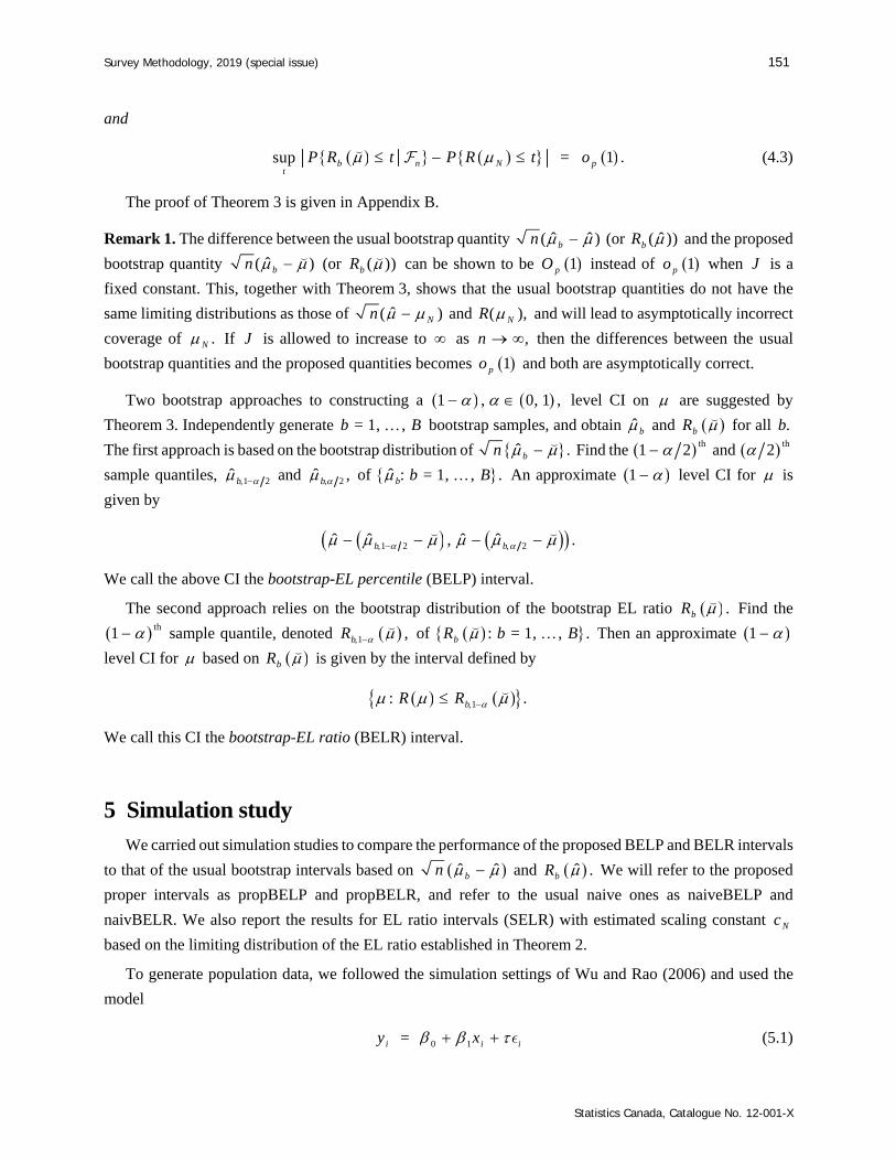
Survey Methodology, 2019 (special issue) 151
Statistics Canada, Catalogue No. 12-001-X
and
= 1 .sup b n N pt
P R t P R t o (4.3)
The proof of Theorem 3 is given in Appendix B.
Remark 1. The difference between the usual bootstrap quantity ˆ ˆ( )bn (or ˆ( ))bR and the proposed
bootstrap quantity ˆ( )bn (or ( ))bR can be shown to be 1pO instead of 1po when J is a
fixed constant. This, together with Theorem 3, shows that the usual bootstrap quantities do not have the
same limiting distributions as those of ˆ( )Nn and ( ),NR and will lead to asymptotically incorrect
coverage of .N If J is allowed to increase to as ,n then the differences between the usual
bootstrap quantities and the proposed quantities becomes 1po and both are asymptotically correct.
Two bootstrap approaches to constructing a 1 , 0, 1 , level CI on are suggested by
Theorem 3. Independently generate = 1, ,b B bootstrap samples, and obtain ˆ b and bR for all .b
The first approach is based on the bootstrap distribution of ˆ .bn Find the th1 2 and th2
sample quantiles, ,1 2ˆ b and , 2ˆ ,b of ˆ : = 1, , .b b B An approximate 1 level CI for is
given by
,1 2 , 2ˆ ˆ ˆ ˆ, .b b
We call the above CI the bootstrap-EL percentile (BELP) interval.
The second approach relies on the bootstrap distribution of the bootstrap EL ratio .bR Find the
th1 sample quantile, denoted ,1 ,bR of : = 1, , .bR b B Then an approximate 1
level CI for based on bR is given by the interval defined by
,1: .bR R
We call this CI the bootstrap-EL ratio (BELR) interval.
5 Simulation study
We carried out simulation studies to compare the performance of the proposed BELP and BELR intervals
to that of the usual bootstrap intervals based on ˆ ˆbn and ˆ .bR We will refer to the proposed
proper intervals as propBELP and propBELR, and refer to the usual naive ones as naiveBELP and
naivBELR. We also report the results for EL ratio intervals (SELR) with estimated scaling constant Nc
based on the limiting distribution of the EL ratio established in Theorem 2.
To generate population data, we followed the simulation settings of Wu and Rao (2006) and used the
model
0 1=i i iy x (5.1)

152 Cai and Rao: Empirical likelihood inference for missing survey data under unequal probability sampling
Statistics Canada, Catalogue No. 12-001-X
for = 1, , ,i N where 0 1= = 1, ix were generated from an exponential distribution with rate 1, and
i were generated from 21 1 distribution to have a zero mean. The ix were used as the size measure for
selecting PPS samples. The value of was chosen so that the correlation : ,y x between the
variable of interest y and the size measure x reaches a certain level. The finite populations so generated
were held fixed under repeated independent simulation runs. In each particular case of the simulation study,
the number of simulation runs was set to be 10,000, and the number of bootstrap replications in each
simulation run was set to =B 3,000. In Sections 5.1 and 5.2, we focus on constructing 95% CIs for the
population mean of ;y in Section 5.3, we consider 95% CIs for the population distribution function of y
evaluated at given values.
5.1 Case 1: Single imputation class
We first considered the simple case where there is only one imputation class for the entire population.
We set the population size to be =N 5,000, and drew PPS samples with replacement from the population
generated from model (5.1). The value in model (5.1) was chosen such that = 0.3. The sample size
was set to =n 80 and 250, and for each sample size, we examined two settings of response probability,
=P 0.4 and 0.8. For each combination of n and ,P we used two settings for the number of draws in
imputation, = 1J and 5. Note that, unlike the original setting used by Wu and Rao (2006), where a constant
was added to all the size measures to avoid extremely small values, we intentionally avoided adding any
constant to the size measures to test the case where inclusion probabilities contain very small values and
differ largely in size.
The coverage probabilities and average lengths of the proposed and naive bootstrap-EL intervals for the
population mean are shown in Table 5.1. When = 1,J it is clear that in all the cases the proposed propBELR
intervals have the most accurate coverage probabilities and shorter average lengths than the naiveBELR
intervals. The naivBELR intervals show 1%-2% of over-coverage relative to the 95% nominal coverage.
Both propBELP and naivBELP intervals perform much worse than the BELR intervals in terms of coverage
probability, and show serious under-coverage. The propBELP intervals, however, have much better
coverage probabilities than the naivBELP intervals. The naivBELP and propBELP intervals can be shown
to have exactly the same lengths, so their lengths are shown in a single column titled “BELP” under
“Average Length” in Table 5.1 and also in the other tables. Given that both the propBELP and naiveBELP
intervals have notable under-coverage, their lengths are not comparable to those of the BELR intervals.
Moreover, when sample size increases, all the BELP intervals show improved coverage probabilities, while
the coverages of the BELR intervals are stable in terms of change in the sample size. The SELR intervals
also show significant under-coverage, although they have slightly better coverage than the propBELP
intervals. The average lengths of all the intervals decrease as the sample size increases.

Survey Methodology, 2019 (special issue) 153
Statistics Canada, Catalogue No. 12-001-X
Table 5.1 95% CIs for the population mean: single imputation class case
J n 1P Coverage probability Average length
SELR naivBELP propBELP naivBELR propBELR SELR BELP naivBELR propBELR1 80 0.4 0.880 0.785 0.832 0.965 0.951 3.094 3.081 4.416 4.199
0.8 0.897 0.828 0.863 0.961 0.948 2.404 2.331 3.200 3.062 250 0.4 0.900 0.827 0.886 0.966 0.951 2.161 2.069 2.832 2.646
0.8 0.913 0.862 0.904 0.960 0.947 1.617 1.558 2.068 1.972 5 80 0.4 0.874 0.804 0.816 0.946 0.944 3.317 2.864 4.339 4.277
0.8 0.890 0.850 0.858 0.947 0.944 2.339 2.222 3.074 3.038 250 0.4 0.901 0.864 0.877 0.947 0.945 2.286 1.925 2.792 2.742
0.8 0.908 0.889 0.902 0.948 0.946 1.567 1.463 1.939 1.914
When J is increased to 5, the differences between the naivBELR and propBELR intervals, and those
between the naivBELP and propBELP intervals, become nearly negligible. This observation agrees with
our theoretical finding given in Remark 1, that is, as J increases, the differences between the proposed
intervals and naive intervals will diminish as .n The average lengths of the propBELR intervals
remain slightly shorter than those of the naivBELR intervals. The coverage probabilities of both the
propBELR intervals and the SELR intervals do not change substantially as J increases from 1 to 5.
A striking observation is that the BELP intervals perform much worse than the BELR intervals.
Unreported simulation studies suggest that this is likely due to the use of unequal probability sampling.
When simple random sampling is used, the performance of the propBELP interval is found to be close to
that of the propBELR interval, which is also observed by Cai et al. (2019). In addition, if a constant is added
to the size measures to avoid extremely small values, we observed that the performance of the proposed
propBELP interval increases greatly while that of the naivBELP increases slightly. This is further illustrated
in the simulation study presented in Section 5.2. A clear advantage of the proposed BELR interval over the
proposed BELP interval is that the performance of the BELR interval is not significantly affected by the
variation in inclusion probabilities.
The above simulation results show that the naivBELR intervals have similar performance to the
propBELR intervals with a slight over-coverage. Does this imply that the naivBELR interval is also
asymptotically correct? To answer this question, we conducted a large-sample simulation study. In this
study, we set the population size to be =N 25,000, and considered sample sizes =n 500, 1,000, 1,500,
2,000 and 3,000. The population data were generated from model (5.1) and PPS samples were drawn with
replacement from the population repeatedly and independently. The response probability P was fixed at
0.8 and the number of random draws J in the imputation was set to 1.
The simulation results based on large samples are reported in Table 5.2. In all the cases, the coverage
probabilities of the propBELR intervals are precisely 95%. However, the naivBELR intervals always exihbit
1%-1.5% of over-coverage regardless of how large the sample size is. This shows that the naivBELR
intervals are asymptotically biased. The coverage probabilities of the propBELP intervals improve as the
sample size increases, and when n is beyond 2,000, they are satisfactorily close to the nominal coverage of
95%. The naivBELP intervals, however, have lower than 90% coverage probabilities in all the cases,
implying that they are asymptotically incorrect. The SELR intervals also improve as the sample size n
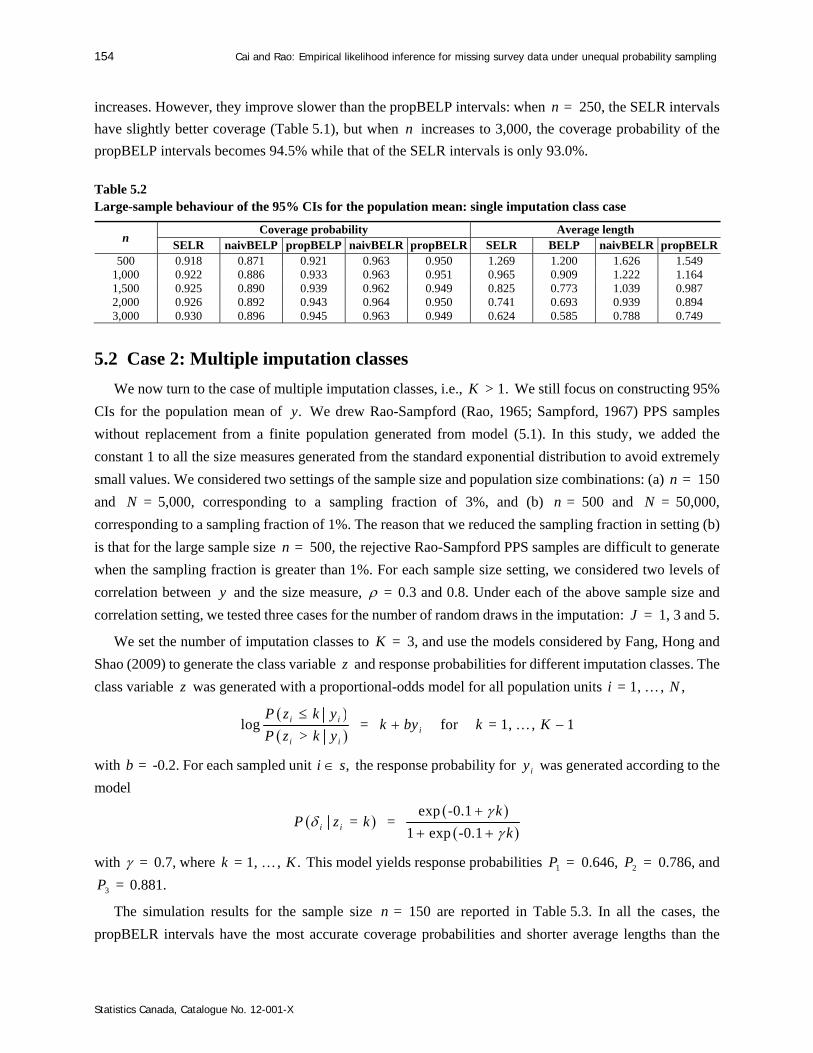
154 Cai and Rao: Empirical likelihood inference for missing survey data under unequal probability sampling
Statistics Canada, Catalogue No. 12-001-X
increases. However, they improve slower than the propBELP intervals: when =n 250, the SELR intervals
have slightly better coverage (Table 5.1), but when n increases to 3,000, the coverage probability of the
propBELP intervals becomes 94.5% while that of the SELR intervals is only 93.0%.
Table 5.2 Large-sample behaviour of the 95% CIs for the population mean: single imputation class case
n Coverage probability Average length
SELR naivBELP propBELP naivBELR propBELR SELR BELP naivBELR propBELR500 0.918 0.871 0.921 0.963 0.950 1.269 1.200 1.626 1.549
1,000 0.922 0.886 0.933 0.963 0.951 0.965 0.909 1.222 1.164 1,500 0.925 0.890 0.939 0.962 0.949 0.825 0.773 1.039 0.987 2,000 0.926 0.892 0.943 0.964 0.950 0.741 0.693 0.939 0.894 3,000 0.930 0.896 0.945 0.963 0.949 0.624 0.585 0.788 0.749
5.2 Case 2: Multiple imputation classes
We now turn to the case of multiple imputation classes, i.e., > 1.K We still focus on constructing 95%
CIs for the population mean of .y We drew Rao-Sampford (Rao, 1965; Sampford, 1967) PPS samples
without replacement from a finite population generated from model (5.1). In this study, we added the
constant 1 to all the size measures generated from the standard exponential distribution to avoid extremely
small values. We considered two settings of the sample size and population size combinations: (a) =n 150
and =N 5,000, corresponding to a sampling fraction of 3%, and (b) =n 500 and =N 50,000,
corresponding to a sampling fraction of 1%. The reason that we reduced the sampling fraction in setting (b)
is that for the large sample size =n 500, the rejective Rao-Sampford PPS samples are difficult to generate
when the sampling fraction is greater than 1%. For each sample size setting, we considered two levels of
correlation between y and the size measure, = 0.3 and 0.8. Under each of the above sample size and
correlation setting, we tested three cases for the number of random draws in the imputation: =J 1, 3 and 5.
We set the number of imputation classes to =K 3, and use the models considered by Fang, Hong and
Shao (2009) to generate the class variable z and response probabilities for different imputation classes. The
class variable z was generated with a proportional-odds model for all population units = 1, , ,i N
log = for = 1, , 1>
i ii
i i
P z k yk by k K
P z k y
with =b -0.2. For each sampled unit ,i s the response probability for iy was generated according to the
model
exp 0.1= =
1 exp -0.1
-i i
kP z k
k
with = 0.7, where = 1, , .k K This model yields response probabilities 1 =P 0.646, 2 =P 0.786, and
3 =P 0.881.
The simulation results for the sample size =n 150 are reported in Table 5.3. In all the cases, the
propBELR intervals have the most accurate coverage probabilities and shorter average lengths than the

Survey Methodology, 2019 (special issue) 155
Statistics Canada, Catalogue No. 12-001-X
naivBELR intervals. The naivBELR intervals show over-coverage when = 1,J and their coverages
improve as J increases. The coverage probabilities of the propBELP intervals are lower than the nominal
level, but are much improved compared to the serious under-coverage that we have observed in the
simulation study of Section 5.1 where no constant was added to the size measures to avoid extremely small
values. The SELR intervals exhibit slight under-coverage when = 0.3; they perform equally well as the
propBELR intervals when = 0.8. The naivBELP intervals perform the worst with significant under-
coverage in all the cases.
Table 5.3 95% CIs for the population mean: multiple imputation classes case =n 150, =N 5,000
J Coverage probability Average length
SELR naivBELP propBELP naivBELR propBELR SELR BELP naivBELR propBELR0.3 1 0.943 0.890 0.930 0.961 0.950 1.379 1.332 1.517 1.439
3 0.945 0.916 0.930 0.954 0.951 1.335 1.281 1.426 1.397 5 0.946 0.919 0.930 0.953 0.950 1.327 1.271 1.410 1.390
0.8 1 0.953 0.899 0.946 0.967 0.952 0.471 0.465 0.502 0.474 3 0.951 0.928 0.945 0.956 0.950 0.455 0.444 0.464 0.453 5 0.951 0.935 0.945 0.956 0.952 0.447 0.440 0.455 0.449
The simulation results for the larger sample size =n 500 are shown in Table 5.4. As in the case of the
smaller sample size =n 150, the propBELR and propBELP intervals outperform their naive counterparts,
and the propBELR intervals perform better than the propBELP intervals in terms of coverage probability.
Under both sample sizes, 150 and 500, the coverage probabilities of the propBELR intervals are nearly
identical to the nominal level, and those of the propBELP intervals improve as the sample size increases,
suggesting that the proposed BELR and BELP intervals are asymptotically correct. However, the coverage
probabilities of the naivBELR and naivBELP intervals do not improve as the sample size increases,
indicating that they are asymptotically incorrect. The SELR intervals have approximately the same
performance as the propBELR intervals in terms of both coverage probabilities and average lengths under
the large sample size setting.
Table 5.4 95% CIs for the population mean: multiple imputation classes case =n 500, =N 50,000
J Coverage probability Average length
SELR naivBELP propBELP naivBELR propBELR SELR BELP naivBELR propBELR0.3 1 0.949 0.895 0.939 0.960 0.948 0.747 0.734 0.795 0.754
3 0.948 0.926 0.941 0.954 0.949 0.720 0.704 0.742 0.727 5 0.949 0.933 0.942 0.952 0.950 0.719 0.698 0.731 0.721
0.8 1 0.949 0.898 0.947 0.964 0.949 0.260 0.258 0.276 0.260 3 0.949 0.931 0.949 0.957 0.952 0.248 0.246 0.254 0.248 5 0.950 0.937 0.946 0.954 0.949 0.246 0.244 0.250 0.246
It is worth noting that the average lengths of all the intervals are shorter when the correlation between
y and the size measure is higher. This agrees with the classical estimation theory of survey sampling that
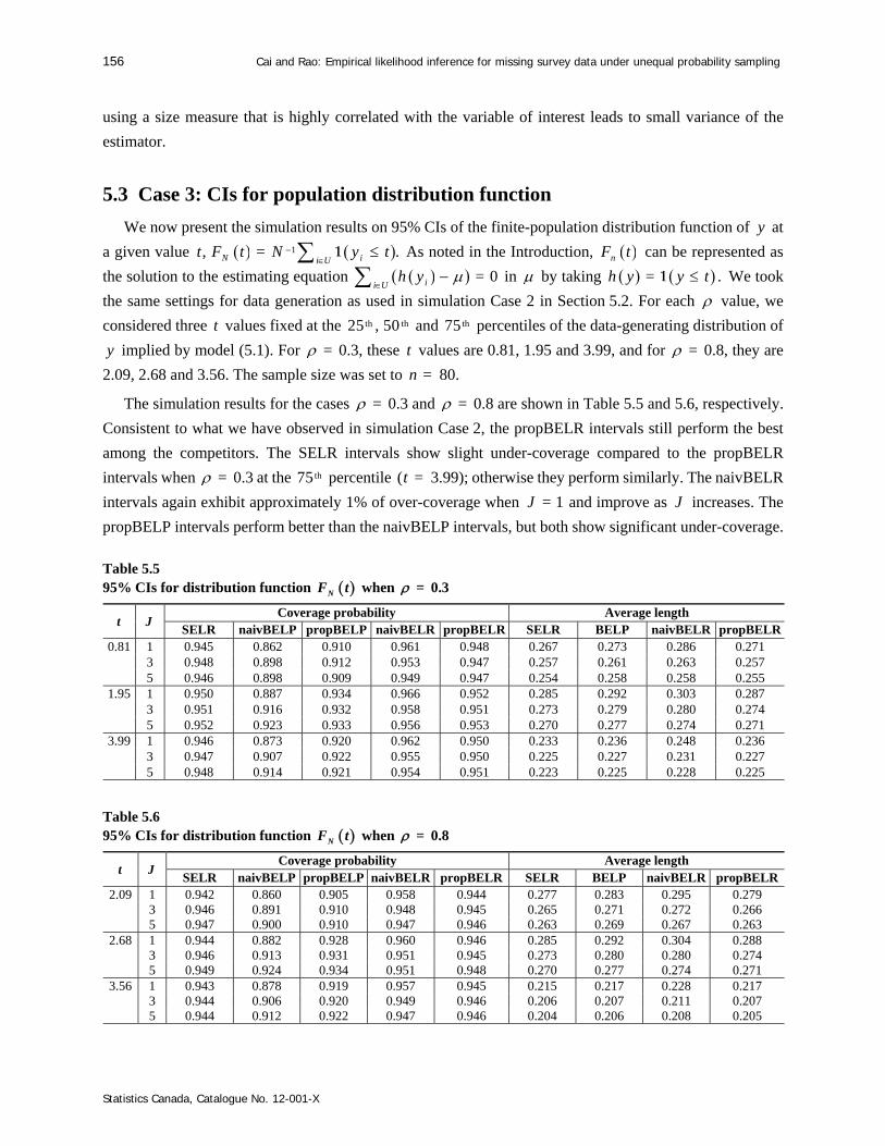
156 Cai and Rao: Empirical likelihood inference for missing survey data under unequal probability sampling
Statistics Canada, Catalogue No. 12-001-X
using a size measure that is highly correlated with the variable of interest leads to small variance of the
estimator.
5.3 Case 3: CIs for population distribution function
We now present the simulation results on 95% CIs of the finite-population distribution function of y at
a given value ,t 1= .N ii UF t N y t
1 As noted in the Introduction, nF t can be represented as
the solution to the estimating equation = 0ii Uh y
in by taking = .h y y t1 We took
the same settings for data generation as used in simulation Case 2 in Section 5.2. For each value, we
considered three t values fixed at the th25 , th50 and th75 percentiles of the data-generating distribution of
y implied by model (5.1). For = 0.3, these t values are 0.81, 1.95 and 3.99, and for = 0.8, they are
2.09, 2.68 and 3.56. The sample size was set to =n 80.
The simulation results for the cases = 0.3 and = 0.8 are shown in Table 5.5 and 5.6, respectively.
Consistent to what we have observed in simulation Case 2, the propBELR intervals still perform the best
among the competitors. The SELR intervals show slight under-coverage compared to the propBELR
intervals when = 0.3 at the th75 percentile ( =t 3.99); otherwise they perform similarly. The naivBELR
intervals again exhibit approximately 1% of over-coverage when = 1J and improve as J increases. The
propBELP intervals perform better than the naivBELP intervals, but both show significant under-coverage.
Table 5.5 95% CIs for distribution function NF t when = 0.3
t J Coverage probability Average length
SELR naivBELP propBELP naivBELR propBELR SELR BELP naivBELR propBELR0.81 1 0.945 0.862 0.910 0.961 0.948 0.267 0.273 0.286 0.271
3 0.948 0.898 0.912 0.953 0.947 0.257 0.261 0.263 0.257 5 0.946 0.898 0.909 0.949 0.947 0.254 0.258 0.258 0.255
1.95 1 0.950 0.887 0.934 0.966 0.952 0.285 0.292 0.303 0.287 3 0.951 0.916 0.932 0.958 0.951 0.273 0.279 0.280 0.274 5 0.952 0.923 0.933 0.956 0.953 0.270 0.277 0.274 0.271
3.99 1 0.946 0.873 0.920 0.962 0.950 0.233 0.236 0.248 0.236 3 0.947 0.907 0.922 0.955 0.950 0.225 0.227 0.231 0.227 5 0.948 0.914 0.921 0.954 0.951 0.223 0.225 0.228 0.225
Table 5.6 95% CIs for distribution function NF t when = 0.8
t J Coverage probability Average length
SELR naivBELP propBELP naivBELR propBELR SELR BELP naivBELR propBELR2.09 1 0.942 0.860 0.905 0.958 0.944 0.277 0.283 0.295 0.279
3 0.946 0.891 0.910 0.948 0.945 0.265 0.271 0.272 0.266 5 0.947 0.900 0.910 0.947 0.946 0.263 0.269 0.267 0.263
2.68 1 0.944 0.882 0.928 0.960 0.946 0.285 0.292 0.304 0.288 3 0.946 0.913 0.931 0.951 0.945 0.273 0.280 0.280 0.274 5 0.949 0.924 0.934 0.951 0.948 0.270 0.277 0.274 0.271
3.56 1 0.943 0.878 0.919 0.957 0.945 0.215 0.217 0.228 0.217 3 0.944 0.906 0.920 0.949 0.946 0.206 0.207 0.211 0.207 5 0.944 0.912 0.922 0.947 0.946 0.204 0.206 0.208 0.205

Survey Methodology, 2019 (special issue) 157
Statistics Canada, Catalogue No. 12-001-X
6 Conclusion and future perspectives
A fractional imputation is proposed and an associated EL is developed for making inference on the
population mean of a function of a variable of interest for survey data that are missing at random under
PPS sampling with negligible sampling fractions or with replacement. Two bootstrap and EL based
methods, BELP and BELR, are proposed for constructing CIs on , and are shown to be asymptotically
correct. Simulation studies show that the proposed intervals perform better than their naive bootstrap
counterparts under various sample size settings. In addition, the proposed BELR intervals are seen to have
more accurate coverage probabilities than those of the proposed BELP intervals, particularly in two
situations: (i) when the inclusion probabilities differ in size substantially, or (ii) when the sample size is not
too large. Moreover, the proposed BELR intervals exhibit notably better coverage probabilities than the EL-
ratio intervals with estimated scaling constant (SELR intervals) in the above case (i).
For parameters defined by smooth estimating equations under an IID setting, Tang and Qin (2012), using
an inverse-probability-weighted fractional imputation, achieved two most desirable properties of EL
inference with data missing at random: (1) the associated MELE attains the semi-parametric efficiency
bound, and (2) the corresponding EL ratio follows a simple chi-square limiting distribution. However, their
method requires both the observed and the missing data to be imputed, which is unlikely to be accepted in
practice in survey studies. We are working on extending Tang and Qin (2012) to a survey setup while
avoiding imputing observed data points.
Our future work also includes extending the current methods to tackling missing data from stratified
sampling and multistage sampling, as well as to the case where the sampling fraction is non-negligible.
Appendix A
Define, for all = 1, , ,k K
1
1
= = ,
= = ,
k i ii U
k i i Ni U
Q z k nd
H N z k h y
1
1
and
22 21= = .kH i i N i k k
i U
S N z k h y nd N H Q
1
Theorems 1-3 are established under the following regularity conditions.
(R.1) ,kQ kH and 2kHS converge to some constant limits as N for all = 1, , ;k K 0kQ
for all k and 2 0kHS for at least one .k
(R.2) There exists a constant > 0 such that (a) 21 = 1 ,i Ni UN h y O
and (b)
1 = 1ii UN d o
as .N
158 Cai and Rao: Empirical likelihood inference for missing survey data under unequal probability sampling
Statistics Canada, Catalogue No. 12-001-X
(R.3) 1 2= .max i s i i N pd h y o n
Conditions (R.1) and (R.2) ensure that the population has regular behaviour when embedded in a
asymptotic sequence. Condition (R.3) is a standard condition in EL inference as used by Chen and Sitter
(1999).
The constant N in Theorem 1 is given by the positive square root of
1 2 22 1
=1
= 1 .k
K
N k k H k kk
P P J S H Q
The constant Nc in Theorem 2 is given by
2
2 21=1
= .1
k
NN K
k k H k kk
cP P J S H Q
Design-consistent estimators of 2N and Nc can be obtained by plugging in the following design-consistent
estimators of ,kP ,kQ KH and 2kHS for = 1, , :k K
1
11
22 1 1 21 2
=ˆˆ = , = = ,
=
ˆ ˆ= = ,
ˆˆ ˆˆ= = .k
i i ii sk k i
i si ii s
k k i i i ii s
H k i i i i k ki s
z k dP Q n z k
z k d
H N P z k d h y
S N P z k h y nd N Q H
11
1
1
1
Appendix B
We now give proofs for Theorems 1-3. Let E and Var denote the expectation and variance
operators with respect to the sampling design, respectively. We consider PPS sampling with replacement in
the proofs. All results also apply to PPS sampling without replacement with negligible sampling fractions.
Lemma 1. Under condition (R.1), 1= = 1 .k k k pn r P o
Proof of Lemma 1. Recall that = = ,k ii sn z k
1 so we have 1E = = =k i ii U
n n z k nd
1
= 1kQ O by (R.1). Under PPS sampling with replacement, we have
1 21 2 1Var = = E = = 1 .k i i k k ki U
n n n z k nd n n n Q Q o
1
Therefore, by Markov’s inequality, we easily obtain = E 1 = 1 .k k p k pn n n n o Q o
Moreover, since = = ,k i ii sr z k
1 by the MAR assumption, we have E =kr n
E = E = E = .i i k k k k kz k n n P n n P Q Similar to the case of ,kn n we can show that
Var = 1 ,kr n o so we have = 1 .k k k pr n P Q o
Survey Methodology, 2019 (special issue) 159
Statistics Canada, Catalogue No. 12-001-X
We hence conclude that 1= = 1 .k k k k k pn r n n r n P o
Lemma 2. Under conditions (R.1) and (R.2),
1 1 0, 1 .d
N i Ni s
nN h N
Proof of Lemma 2. The following decomposition holds:
1 = ,i N n ni s
nN h U V
where 1= En i N i N ni sU nN h h
and 1= E .n i N ni s
V nN h Noting
that 1=1
ˆE = = 1 ,K
i N n i i i i N i k krkh z k d h y r H 1 where ˆ =krH
= ,i i i i Ni sz k d h y
1 we get
=1
ˆ= and =K
kn i n kr
i s k k
n n nU V H
N N r
(B.1)
with
11 * *
=1 =1
ˆ= 1 = .K J
i i i ij ij N k krk j
z k J d h y r H 1
We now work out the conditional limiting distributions of nU given the sample data .n Since the
imputation is carried out independently across ,i s i are conditionally independent random variables
given .n Note that i have zero conditional mean, = 0i nE and common conditional variance for
all .i s Moreover, we have
2
222
=1
ˆ1Var = 1 = .
Kk kr
n n i i i i Nk i sk k
n n n HU z k d h y
r J N r N
1
By Lemma 1, 1= 1 ,k k k pn r P o and in the proof of Lemma 1, we have shown
1 1= 1 .k k k pn r P Q o Under condition (R.2)(a), we can show that
2222
1= = = 1i i i i N k i i N i p
i s i s
nz k d h y P z k h y nd N o
N N
1 1
and ˆ = 1 .kr k k pH N P H o Therefore,
22 1
=1
:= Var = 1 1 = 1 .k
K
u n n k H p pk
s U P J S o O (B.2)
By the Berry-Essen Theorem (Chow and Teicher, 1997, Section 9.1), we have
2 ,sup n u n u ut
P U ts t c s
160 Cai and Rao: Empirical likelihood inference for missing survey data under unequal probability sampling
Statistics Canada, Catalogue No. 12-001-X
where 0, and c are some constants that do not rely on ,n and
2 2
22 1 2
2
1= E = E .u i n i n
i s i s
nnN
N n
We can further show that, under condition (R.2)(a), 1 2E = 1 ,i n pi sn O
which implies that
2 = 1 .u po Therefore,
= 1 .sup n u n pt
P U ts t o (B.3)
We next find the limiting distribution of .nV It can be shown that, for each = 1, , ,k K
1 21 1ˆ = = .k i k k
kr i i i N pi sk k k k
n n H HH z k d h y o n
N r n P N Q Q
1
Hence, by (B.1), we have = 1 ,nn i pn i s
V o
where
=1
= = .K
i k ki i i i N
k k k k
n H Hz k d h y
P N Q Q
1
Under sampling with replacement, ,i ,i s are independent random variables. Moreover, we get
E = 0ii s
and
1 2 22
=1
:= Var = .k
K
v n k H k kk
s V P S H Q (B.4)
Under condition (R.2)(a), the conditions of the Lyanunov central limit theorem are satisfied, so we have
1 0, 1 .d
v ns V N (B.5)
By (B.3) and (B.5), and observing that v us s converges to a constant limit under condition (R.1), all
conditions of Theorem 2 of Chen and Rao (2007) are verified. Accordingly, we have
1 22 2 0, 1 .d
u v n ns s U V N
Noticing that 2 2 2= 1u v N ps s o and 1= ,n n i Ni sU V nN h
the claimed result is proved.
Proof of Theorem 1. By (3.3) and (2.1), we have
1ˆ = ,N i Ni s
n nd h
(B.6)
where 1 *=1 =1
= = 1 .K J
i i i i iji s k jd z k d J d
1
Note that, given the sample data ,n 1 1=1
E = = .K
n k k i i ik i sN d N n r z k d
1 By
Lemma 1, we have 1= 1 .k k k pn r P o Moreover, we can show that, under condition (R.2)(b),

Survey Methodology, 2019 (special issue) 161
Statistics Canada, Catalogue No. 12-001-X
1 1
1
= = E = 1
= = 1 .
i i i i i i pi s i s
k i pi U
N z k d N z k d o
N P z k o
1 1
1
Therefore,
11 1
=1
E = = 1 = 1 1 .K
n k k i p pk i U
N d P N P z k o o
1
In addition, it can be shown that given ,n 1 1= E 1 .n pN d N d o The above results imply that
1 = 1 1 .pN d o (B.7)
Combining (B.6), (B.7) and Lemma 2, we obtain the desired result.
Proof of Theorem 2. By (3.2) and (3.4), we have
= 2 = 2 log 1 .N n N N i Ni s
R l h
(B.8)
where N satisfies 1 1 = 0.i N N i Ni sn h h
Using the same argument as used by Owen
(2001, Section 11.2, Proof of Theorem 3.2), we can show that, under condition (R.3), 1 2=N pO n and
1 22
= .i Ni s
N pi Ni s
ho n
h
By this expression of ,N (B.8) and a Taylor’s expansion, we obtain
2 2
21 1
2 2 2
= 2 1
= 1 .
N N i N N i N pi s i s
N i Ni sp
i N Ni s
R h h o
nN ho
nN h
(B.9)
Note that 2 21 2= ,i Ni s
nN h A A
where
2 211
=1
= = ,K
i i i N ii s k
A n z k h y nd N
1
and
2
1 2 * *2
=1 =1
= 1 = .K J
i i ij N iji s k j
A n z k J h y nd N
1
Under condition (R.2)(a), we can show that 2 21 =1
= 1k
K
k H k k pkA P S H Q o and 2 =A
2 21=1
1 1 .k
K
k H k k pkP J S H Q o Hence,
2 22 2 1
=1
= 1 1 .k
K
i N k k H k k pi s k
nN h P P J S H Q o

162 Cai and Rao: Empirical likelihood inference for missing survey data under unequal probability sampling
Statistics Canada, Catalogue No. 12-001-X
Theorem 2 is then proved by substituting the above expression into (B.9) and applying Theorem 1.
For the proof of Theorem 3, we introduce the following Lemma.
Lemma 3. Under conditions (R.1) and (R.2),
1 1,
=1
= 1 .supn
N b i N N n pt i
P nN h h t t o
where = .N i Ni sh h
Proof of Lemma 3. Let ,b n denote the bootstrap sample , , , ,( , , , ) : = 1, , .b i b i b i b iy d z i n We have the
following decomposition:
1,
=1
= ,n
b i N n ni
nN h
where 1, , ,=1
= En
n b i N b i N b ninN h h and
1, ,
=1
= E .n
n b i N b n Ni
nN h h
Similar to the proof of Lemma 2, we can show that
, = 1 ,sup n u b n pt
P ts t o (B.10)
where us is defined in (B.2).
We next give the conditional limiting distribution of n given .n It can be shown that
1,=1
= 1 ,n
n b i pinN o where
1 1 1 1, , , , , ,
=1
ˆ ˆ= = = .K
b i k b i b i b i b i N k kr b i k kr Nk
P z k d h y r H z k r H n h
1 1
Conditioned on ,n ,b i are IID across = 1, , ,i n and we can show that ,E = 0b i n and
2
2, 2
=1 =1
2
2=1
1 ˆVar = =
1 ˆ .
n K
b i n k i i i i N kri k i s k
K
k krk k
n nP z k d h y H
N N r
nn H
N r
1
We can show that the first term on the right hand side (RHS) equals 1 2=1
1k
K
k H pkP S o and the second
term on the RHS equals 2=1
1 .K
k k pkH Q o Therefore
1 2 21 2,
=1 =1
Var = 1 = 1 ,k
n K
b i n k H k k p v pi k
nN P S H Q o s o

Survey Methodology, 2019 (special issue) 163
Statistics Canada, Catalogue No. 12-001-X
where 2vs is defined in (B.4). By verifying the conditions of the Berry-Essen Theorem as in the proof of
Lemma 2, we get
= 1 .sup n v n pt
P ts t o (B.11)
By (B.10) and (B.11), and applying Theorem 2 of Chen and Rao (2007), we obtain the claimed results.
Proof of Theorem 3. We first prove (4.2). By (3.3) and (2.1), we have
1,
=1
ˆ = ,n
b N b b i Ni
n nd h
where 1 *, , , , ,=1 =1 =1
= = 1 .n K J
b b i b i b i b i b iji k jd z k d J d 1 By (4.1), we have
1 1= = ,N i N Ni s
n nd h nd h
where =1
= = .K
k k i i ii s kd n r z k d
1
It is straightforward to show that = 1b pd N d N o and = 1 1pd N o
under condition
(R.2)(b). Therefore,
1 1,
=1
ˆ = 1 .n
b b i N N pi
nN nN h h o
Then, by Lemma 3, we have
1 ˆ = 1 .sup b N n pt
P nN t t o
This, combined with Theorem 1 and Polya’s Theorem, completes the proof of (4.2).
The result (4.3) can be proved based on (4.2) and by following the same arguments as used in the proof
of Theorem 2.
References
Brick, J.M., and Kalton, G. (1996). Handling missing data in survey research. Statistical Methods in Medical Research, 5(3), 215-238.
Cai, S., Qin, Y., Rao, J.N.K. and Winiszewska, M. (2019). Empirical likelihood confidence intervals under
imputation for missing survey data from stratified random sampling. To appear in The Canadian Journal of Statistics.
Chen, S., and Kim, J.K. (2014). Population empirical likelihood for nonparametric inference in survey
sampling. Statistica Sinica, 24(1), 335-355. Chen, J., and Rao, J.N.K. (2007). Asymptotic normality under two-phase sampling designs. Statistica
Sinica, 17, 1047-1064.

164 Cai and Rao: Empirical likelihood inference for missing survey data under unequal probability sampling
Statistics Canada, Catalogue No. 12-001-X
Chen, J., and Sitter, R.R. (1999). A pseudo empirical likelihood approach to the effective use of auxiliary information in complex surveys. Statistica Sinica, 9(2), 385-406.
Chow, Y.S., and Teicher, H. (1997). Probability Theory: Independence, Interchangeability, Martingales,
3rd Edition. New York: Springer. Fang, F., Hong, Q. and Shao, J. (2009). A pseudo empirical likelihood approach for stratified samples with
nonresponse. Annals of Statistics, 37(1), 371-393. Haziza, D., and Beaumont, J.-F. (2007). On the construction of imputation classes in surveys. International
Statistical Review, 75(1), 25-43. Kalton, G., and Kish, L. (1984). Some efficient random imputation methods. Communications in Statistics -
Theory and Methods, 13(16), 1919-1939. Owen, A.B. (1988). Empirical likelihood ratio confidence intervals for a single functional. Biometrika,
75(2), 237-249. Owen, A.B. (2001). Empirical Likelihood. New York: Chapman and Hall. Platek, R., and Gray, G.B. (1983). Imputation methodology: Total survey error. In Incomplete Data in
Sample Survey, (Eds., W.G. Madow, I. Olkin and D.B. Rubin), New York: Academic Press, 249-333. Qin, J., and Lawless, J. (1994). Empirical likelihood and general estimating equations. The Annals of
Statistics, 22(1), 300-325. Rao, J.N.K. (1965). On two simple schemes of unequal probability sampling without replacement. Journal
of the Indian Statistical Association, 3, 173-180. Rao, J.N.K., and Shao, J. (1992). Jackknife variance estimation with survey data under hot deck imputation.
Biometrika, 79(4), 811-822. Sampford, M.R. (1967). On sampling without replacement with unequal probabilities of selection.
Biometrika, 54(3-4), 499-513. Shao, J., and Sitter, R. (1996). Bootstrap for imputed survey data. Journal of American Statistical
Association, 91(435), 1278-1288. Tang, C.Y., and Qin, Y. (2012). An efficient empirical likelihood approach for estimating equations with
missing data. Biometrika, 99(4), 1001-1007. Wang, D., and Chen, S.X. (2009). Empirical likelihood for estimating equations with missing values. The
Annals of Statistics, 37(1), 490-517. Wu, C., and Rao, J.N.K. (2006). Pseudo-empirical likelihood ratio confidence intervals for complex surveys.
The Canadian Journal of Statistics, 3(3), 359-375.

Survey Methodology, 2019 (special issue) 165 Vol. 45, No. 1, pp. 165-184 Statistics Canada, Catalogue No. 12-001-X
1. Xianpeng Zong, School of Mathematical Sciences, Capital Normal University, Beijing, 100048, China; Rong Zhu, Academy of Mathematics
and Systems Science, Chinese Academy of Sciences, Beijing 100190, China. E-mail: [email protected]; Guohua Zou, School of Mathematical Sciences, Capital Normal University, Beijing, 100048, China.
Improved Horvitz-Thompson estimator in survey sampling
Xianpeng Zong, Rong Zhu and Guohua Zou1
Abstract
The Horvitz-Thompson (HT) estimator is widely used in survey sampling. However, the variance of the HT estimator becomes large when the inclusion probabilities are highly heterogeneous. To overcome this shortcoming, in this paper we propose a hard-threshold method for the first-order inclusion probabilities. Specifically, we carefully choose a threshold value, then replace the inclusion probabilities smaller than the threshold by the threshold. Through this shrinkage strategy, we construct a new estimator called the improved Horvitz-Thompson (IHT) estimator to estimate the population total. The IHT estimator increases the estimation accuracy much although it brings a bias which is relatively small. We derive the IHT estimator’s mean squared error and its unbiased estimator, and theoretically compare the IHT estimator with the HT estimator. We also apply our idea to construct an improved ratio estimator. We numerically analyze simulated and real data sets to illustrate that the proposed estimators are more efficient and robust than the classical estimators.
Key Words: Horvitz-Thompson estimator; Inverse probability weighting; Hard-threshold; Robustness; Unequal
probability sampling; Sampling without/with replacement; Ratio estimator.
1 Introduction
The Horvitz-Thompson (HT) estimator proposed by Horvitz and Thompson (1952) is widely used in
survey sampling. It has also been applied to other fields such as functional data analysis (Cardot and
Josserand, 2011) and the treatment effect (Rosenbaum, 2002). The HT estimator is an unbiased estimator
constructed via inverse probability weighting. However, when the inclusion probabilities are highly
heterogeneous, i.e., inclusion probabilities of some units are relatively tiny, the variance of the HT estimator
becomes large due to inverse probability weighting. In this paper, we propose an improved Horvitz-
Thompson (IHT) estimator to address this problem.
Our approach is to use a hard-threshold for the first-order inclusion probabilities. Specifically, we
carefully choose an inclusion probability as the threshold. The inclusion probabilities that are smaller than
the threshold are replaced by the threshold, while the others remain unchanged. In this way, we obtain the
modified inclusion probabilities, and construct an estimator based on the modified inclusion probabilities
through inverse probability weighting. We call this estimator the IHT estimator. This method looks very
easy but is more efficient than the HT estimator. This hard-threshold approach can be explained as a
shrinkage method. Shrinkage is very commonly used in statistics, such as ridge regression (Hoerl and
Kennard, 1970) and high-dimensional statistics (Tibshirani, 1996). In this paper, we use it to reduce the
negative effect of highly heterogeneous inclusion probabilities. Similar to other shrinkage methods, our
approach introduces a bias, which is proved to be very small, but reduces the variance to a larger extent, so
it improves the estimation efficiency. We will theoretically and numerically show the improvement from
using the modified inclusion probabilities. In addition to the population total estimator, we also extend this
strategy to the ratio estimator, and accordingly, an improved ratio estimator is obtained.
166 Zong, Zhu and Zou: Improved Horvitz-Thompson estimator in survey sampling
Statistics Canada, Catalogue No. 12-001-X
The remainder of the paper is organized as follows. Section 2 introduces the HT estimator and shows its
drawback. Section 3 proposes our modified inclusion probabilities and the resultant IHT estimator. We also
provide the IHT estimator’s properties, and theoretically compare it with the HT estimator in this section.
Section 4 extends our idea to obtain an improved ratio estimator and shows that this modification is efficient.
Section 5 presents numerical evidence from simulations and a real data analysis. Section 6 concludes. Proofs
of theoretical results are given in the Appendix.
2 HT estimator and its drawback
Consider a finite population 1= , , NU U U of size ,N where kU denotes the thk unit. For
simplicity, we write = 1, , , , .U k N For each unit ,k suppose that the value ky of the target
characteristic Y is measured. Our aim is to estimate the total, = ,y kUt y using a sample s of size n
which is randomly drawn from the population .U We implement unequal probability sampling without
replacement. Denote =1
Nk k as the first-order inclusion probabilities and kl k l as the second-order
inclusion probabilities.
Horvitz and Thompson (1952) proposed the HT estimator as follows
HTˆ = .k
k s k
yt
The HT estimator HTt is an unbiased estimator of yt and its variance is
2HT 2
ˆ( ) = ,kk klk l kU U
k lk k l
V t y y y
(2.1)
where 2=kk k k for all k and =kl kl k l for all .k l When the inclusion probabilities are
highly imbalanced, i.e., some ’sk are very small, the variance of the HT estimator may be very large.
3 Improved HT estimator
In this section, we improve the HT estimator in the sense of reducing its mean squared error (MSE). The
resultant estimator is referenced as the IHT estimator. For doing this, we first propose the modified first-
order inclusion probabilities, where the hard-threshold method is used to reduce the effect of those inclusion
probabilities with relatively tiny values.
Definition 1. Let 1 2 N be the ordered values of the first-oder inclusion probabilities
1 2, , , .N Assume that there exists an integer 2K such that 11 .K K We define the
modified first-order inclusion probabilities as follows
*> ,
= 1 .,
k k K
kkK K
k N

Survey Methodology, 2019 (special issue) 167
Statistics Canada, Catalogue No. 12-001-X
From the definition, we partition the finite population into two parts: 1 = : >k KU k with size
,N K and 2 = : k KU k with size .K For 1 ,U the first-order inclusion probabilities remain
unchanged, while all of first-order inclusion probabilities for 2U are replaced by .K From this hard-
threshold, we get our modified first-order inclusion probabilities *=1 .N
k k Obviously, the choice of K is
very important. In Section 3.2, we shall provide a simple way to choose .K
Remark on existence of .K The assumption in Definition 1 is quite weak. If 2 > 1 2 1 , then the
sampling fraction 1 13 3> .Nf However that situation that 1
3>f rarely happens in practical surveys.
Thus, the inequality that 2 1 2 1 generally holds.
Instead of the original first-order inclusion probabilities =1 ,Nk k we use our defined modified first-
order inclusion probabilities *=1
Nk k to construct an improved Horvitz-Thompson (IHT) estimator by
inverse probability weighting.
Definition 2. The IHT estimator is defined as
*
ˆ = .kIHT
k s k
yt
Unlike the unbiased HT estimator, the IHT estimator is biased. However, this modification leads to much
smaller MSE due to reducing the variance. It is worth pointing out that, although we focus on sampling
without replacement in this paper, our modification idea is equally applicable to the Hansen-Hurwitz
estimator (Hansen and Hurwitz, 1943) for sampling with replacement.
3.1 Properties of the IHT estimator
In this section, we derive the properties of the IHT estimator. We first provide the expressions of its bias,
variance, MSE and an unbiased estimator of MSE in Theorem 1. Then we compare the IHT estimator with
the HT estimator in Theorems 2 and 3.
Theorem 1. The bias and variance of the IHT estimator ˆIHTt are expressed as
2
ˆ = 1 ,kIHT kU
K
Bias t y
and
2*2 * *
ˆ = ,kk klIHT k k lU U
k lk k l
Var t y y y
respectively, where = 1 , =kk k k kl kl k l k l as defined before. Therefore, its MSE is
given by
2
2
2*2 * *
ˆ = 1 .k kk klIHT k k k lU U U
k lk k lK
MSE t y y y y
(3.1)

168 Zong, Zhu and Zou: Improved Horvitz-Thompson estimator in survey sampling
Statistics Canada, Catalogue No. 12-001-X
An unbiased estimator of the MSE is
2 2
2
22 2
2*2 * *
ˆ =
,
k k lK K KIHT k k ls s
k klK Kk l
kk klk k ls s
k lk k l
MSE t y y y
y y y
where = , = ,kk kl
k klkk kl
s is the sample set, and 2 2= .s s U
Proof. See Appendix A.1.
To derive the properties of the IHT estimator, we need the following regularity conditions:
Condition C.1. *,> 0, > 0,min mini U i j Ui ij and
< .lim sup max ij i ji j UNarrow
n
Condition C.2. max i U iy C with C a positive constant not depending on .N
Condition C.1 is a common condition imposed on the first-order and second-order inclusion
probabilities. The same conditions are used in Breidt and Opsomer (2000), where further comments on C.1
are provided. Condition C.2 is also a common condition.
Theorem 2. For the HT estimator ˆHTt and the IHT estimator ˆ ,IHTt under the Conditions C.1-C.2, we have
1 1 1ˆ ˆ= 0, = ;HT IHTBias N t Bias N t O n
and
1 1 1 1ˆ ˆ= , = .HT IHTMSE N t O n MSE N t O n
Proof. See Appendix A.2.
From Theorem 2, the squared-bias of our IHT estimator is very small compared to its MSE. Although
our IHT estimator brings a bias to reduce the variance, the price for this is relatively small. The following
theorem theoretically compares the efficiency of the two estimators.
Theorem 3. Under the Conditions C.1-C.2, we have
1 1 1ˆ ˆ .IHT HTMSE N t MSE N t o n (3.2)
Especially, for Poisson sampling, we obtain
1 1ˆ ˆ ,IHT HTMSE N t MSE N t
where the strict inequality is true if there exist 2k l U such that .k k l lK Ky y
Survey Methodology, 2019 (special issue) 169
Statistics Canada, Catalogue No. 12-001-X
Proof. See Appendix A.3.
Theorem 3 shows that, under some mild conditions, the proposed IHT estimator is asymptotically more
efficient than the HT estimator. From the proof in Appendix A.3, the term 1o n in equation (3.2) is due
to the interaction term from the second-order inclusion probabilities. We theoretically bound the term as
1 .o n For Poisson sampling, the term does not exist, so the MSE of the IHT estimator is uniformly not
larger than that of the HT estimator. Empirically, we compare the IHT estimator with the HT estimator in
Section 5.
3.2 The choice of K
The efficiency of the IHT estimator relies on the choice of ,K which provides a control of the variance-
and-bias tradeoff. The choice of K needs to satisfy the condition that < 1 1K K of Definition 1,
since the modified inclusion probabilities would cause large bias when K becomes large. On the other
hand, the improvement of the IHT estimator would not be significant if K is small. In the proofs of
Theorem 3, equation (A.5) provides a lower bound of the main term of 1 1HT IHT
ˆ ˆMSE MSE .N t N t
The lower bound increases as K increases. Therefore, denoting the maximum value
* : 1 1= max ,ii iK we choose *K as the threshold. In practice, we propose the following
algorithm to find the maximum value * .K
1 2
=1
1 111 2
Step i Obtain the ordered inclusion probabilities by sorting
rom small to large.
Step ii Test and modify.
If satisfies and the modified first-order
, ,
f
i> ,
, N
Nk k
j jj jj
Algorithm 1 The choice of
K
1*
1
nclusion
probabilities are d
,
efin
,
ed as
an
, , , ,
d
= ,
= .
j j j j N
j
K j
π
Note that the choice of *K based on Algorithm 1 is not optimal in terms of MSE. However, we simulate
an example in Section 5 where the performance of Algorithm 1 is very close to that of the theoretically ideal
choice.
4 Extension to the ratio estimator
When an auxiliary variable is available, the ratio estimator is usually used to estimate the population
total. In this section, we extend the IHT estimator to the case of ratio estimation.
170 Zong, Zhu and Zou: Improved Horvitz-Thompson estimator in survey sampling
Statistics Canada, Catalogue No. 12-001-X
4.1 Improved ratio estimator
Denote the ratio between the population totals of Y and Z as
= ,y zR t t
where yt and zt are the totals of the finite populations Y and ,Z respectively. Let ˆ = ,k
k
yy s
t
ˆ = ,k
k
zz s
t **ˆ = ,k
k
yy s
t and **ˆ = .k
k
zz s
t The classical estimator and our modified estimator of R
are given by
* * *ˆ ˆˆ ˆ ˆ ˆ= , and = .y z y zR t t R t t
We assume that the population total zt is known. To estimate the population total yt of ,Y the classical
ratio estimator is given by
ˆ ˆ ˆ= .R z y zY t t t
Alternatively, our improved ratio estimator of yt based on the modified inclusion probabilities is expressed
as
* * *ˆ ˆ ˆ= .R z y zY t t t
4.2 Properties of the improved ratio estimator
To show theoretically that the improved ratio estimator *ˆRY is more efficient than the classical ratio
estimator ˆ ,RY we need the following regularity conditions:
Condition C.3. = ,lim nN N c where 0, 1c is a constant.
Condition C.4. 1= ,max i j k U ijk ij k O n and
24 6 3 = .max ijkl ijk l ij k l i j k li j k l U
O n
Condition C.3 is a common condition. The same condition is used in Breidt and Opsomer (2000).
Condition C.4 is a mild assumption on the third-order and fourth-order inclusion probabilities. In
Appendix A.5, we present some frequent examples which satisfy Condition C.4.
Comparing our improved estimators with the classical estimators, we have the following result.
Theorem 4. If Conditions C.1-C.4 are satisfied, and 1 2kc z c for all k U with 1c and 2c some
positive constants, then
* 1ˆ ˆ .MSE R MSE R o n
Furthermore,
1 * 1 1ˆ ˆ .R RMSE N Y MSE N Y o n
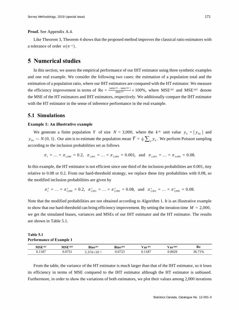
Survey Methodology, 2019 (special issue) 171
Statistics Canada, Catalogue No. 12-001-X
Proof. See Appendix A.4.
Like Theorem 3, Theorem 4 shows that the proposed method improves the classical ratio estimators with
a tolerance of order 1 .o n
5 Numerical studies
In this section, we assess the empirical performance of our IHT estimator using three synthetic examples
and one real example. We consider the following two cases: the estimation of a population total and the
estimation of a population ratio, where our IHT estimators are compared with the HT estimator. We measure
the efficiency improvement in terms of HT IHT
HT
MSE MSE
MSERe = 100%, where HTMSE and IHTMSE denote
the MSE of the HT estimators and IHT estimators, respectively. We additionally compare the IHT estimator
with the HT estimator in the sense of inference performance in the real example.
5.1 Simulations
Example 1: An illustrative example
We generate a finite population Y of size = 3,000,N where the thk unit value 0=k ky y and
0 0, 1 .ky N Our aim is to estimate the population mean 1= .kN UY y We perform Poisson sampling
according to the inclusion probabilities set as follows
1 1,000 1,001 2,000 2,001 3,000= = = 0.2, = = = 0.001, and = = = 0.08.
In this example, the HT estimator is not efficient since one third of the inclusion probabilities are 0.001, tiny
relative to 0.08 or 0.2. From our hard-threshold strategy, we replace these tiny probabilities with 0.08, so
the modified inclusion probabilities are given by
* * * * * *1 1,000 1,001 2,000 2,001 3,000= = = 0.2, = = = 0.08, and = = = 0.08.
Note that the modified probabilities are not obtained according to Algorithm 1. It is an illustrative example
to show that our hard-threshold can bring efficiency improvement. By setting the iteration time = 2,000,M
we get the simulated biases, variances and MSEs of our IHT estimator and the HT estimator. The results
are shown in Table 5.1.
Table 5.1 Performance of Example 1
HTMSE IHTMSE HTBias IHTBias HTVar IHTVar Re
0.1187 0.0751 5.374 610 0.0723 0.1187 0.0029 36.71%
From the table, the variance of the HT estimator is much larger than that of the IHT estimator, so it loses
its efficiency in terms of MSE compared to the IHT estimator although the HT estimator is unbiased.
Furthermore, in order to show the variations of both estimators, we plot their values among 2,000 iterations

172 Zong, Zhu and Zou: Improved Horvitz-Thompson estimator in survey sampling
Statistics Canada, Catalogue No. 12-001-X
in Figure 5.1. It clearly displays that, although there is small bias for the IHT estimator, its variation is much
less than that of the HT estimator. These observations empirically verify our theoretical results.
Figure 5.1 The plots of both estimators in Example 1.
Example 2: ’si depend on an auxiliary variable
We generate the finite population Y of size = 3,000N as follows: = 3k ky x 23 3 ,ke where kx and ke are independently generated from 0, 2U and 0, 1N respectively,
and 0 1 controling the correlation of Y and .X We consider three sampling methods: Poisson
sampling, PPS sampling and PS sampling. The sampling fraction = =nNf 0.02, 0.04, 0.06, 0.08, 0.10,
0.15, 0.20, 0.30. We report the results in Figure 5.2, where = 0.8, and list the specific Re values of
Figure 5.2 in Table 5.4.
From these results, we get the same observations as Example 1. It indicates that our IHT estimator
outperforms the HT estimator in terms of MSE and that the improvement is generally substantial.
Comparing with Figures 5.2(a), 5.2(b), and 5.2(c), PS sampling obtains the biggest advantage of the IHT
estimator over the HT estimator, followed by PPS sampling and Poisson sampling. We also show the results
for different values under PS sampling in Table 5.2, where the case of =f 0.08 is reported and other
cases are ignored because of the similarity. It is observed from the table that, no matter what value takes,
the IHT estimator has uniformly much less MSE than the HT estimator.
0 500 1,000 1,500 2,000 Replication
Var
ied
valu
e
0.5
1.
0
1.5
2
.0
2.5
True Value HT
Improved HT

Survey Methodology, 2019 (special issue) 173
Statistics Canada, Catalogue No. 12-001-X
Table 5.2 The performance of Example 2 for different values, where = 0.08f
HTMSE IHTMSE HTBias IHTBias HTVar IHTVar Re
0 3.45 210 1.36 210 3.43 510 5.82 410 3.45 210 1.30 210 60.70% 0.1 2.51 210 1.38 210 1.16 510 8.25 410 2.51 210 1.30 210 44.91% 0.3 2.43 210 1.24 210 4.65 610 8.86 410 2.43 210 1.15 210 48.97% 0.5 2.38 210 1.07 210 9.83 610 8.44 410 2.38 210 9.88 310 54.92% 0.8 9.38 310 5.22 310 3.04 710 3.16 410 9.38 310 4.91 310 44.33% 0.9 4.75 310 2.65 310 7.98 610 2.64 410 4.74 310 2.38 310 44.27%
Figure 5.2 The performance of our IHT estimator and the HT estimator in Example 2, where = 0.8. From
left to right: the MSE performance, the squared-bias performance, and the variance performance.
0.02 0.04 0.06 0.08 0.1 0.15 0.2 0.3 0.02 0.04 0.06 0.08 0.1 0.15 0.2 0.3 0.02 0.04 0.06 0.08 0.1 0.15 0.2 0.3
MSE
MSE
MSE
0
.00
0
.01
0
.02
0
.03
0
.04
0.00
0.
01
0
.02
0.
03
0
.04
0.0
0
0.0
2 0
.04
0.
06
0.0
8
0.10
HT HT HT Improved HT Improved HT Improved HT
(a) Poisson sampling
(b) PPS sampling
(c) PS sampling
Sq
uare
d bi
as
Squ
ared
bia
s
Sq
uare
d bi
as
0.0
0
0.0
1
0.0
2
0.0
3
0.0
4
0.
00
0.01
0.0
2
0.03
0.0
4
0
.00
0
.02
0.0
4
0.06
0
.08
0.
10
V
aria
nce
Var
ianc
e
Var
ianc
e 0
.00
0
.01
0
.02
0
.03
0
.04
0.00
0.
01
0
.02
0.
03
0
.04
0.0
0
0.0
2 0
.04
0.
06
0.0
8
0.10
HT HT HT Improved HT Improved HT Improved HT
HT HT HT Improved HT Improved HT Improved HT
0.02 0.04 0.06 0.08 0.1 0.15 0.2 0.3 0.02 0.04 0.06 0.08 0.1 0.15 0.2 0.3 0.02 0.04 0.06 0.08 0.1 0.15 0.2 0.3
0.02 0.04 0.06 0.08 0.1 0.15 0.2 0.3 0.02 0.04 0.06 0.08 0.1 0.15 0.2 0.3 0.02 0.04 0.06 0.08 0.1 0.15 0.2 0.3

174 Zong, Zhu and Zou: Improved Horvitz-Thompson estimator in survey sampling
Statistics Canada, Catalogue No. 12-001-X
Example 2 (continued): The performance of Algorithm 1 and the effect of the outcome’s coefficient
of variation
Here we empirically investigate the performance of Algorithm 1 and the effect of the outcome’s
coefficient of variation on our IHT estimator. We generate a finite population through a linear model with
an intercept: 2= 3 3 3 ,k k ky x e where kx and ke are the same as Example 2. We
set = 1,000,N and control the coefficient of variation of the outcome by varying the intercept term
= 10, 5, 0, 5, 10 . Firstly, we study the performance of Algorithm 1. Note that the optimal choice
optK can be derived via minimizing equation (3.1). We compare the MSE values based on optK and *K
from Algorithm 1, and report the results of =f 0.03 in Table 5.3 and ignore other cases because of the
similarity. From the table, the MSE values based on *K are very close to those based on opt .K It indicates
that Algorithm 1 provides an efficient choice of .K Secondly, we investigate the effect of the outcome’s
coefficient of variation. From the table, the IHT estimator always performs much better than the HT
estimator when takes different values. It indicates that our IHT is robust to the outcome’s coefficient of
variation.
Table 5.3 Performance of Algorithm 1, where = 0.03f
Y *K optK HTMSE *MSEK
optMSE Re
-10 -7.80 125 166 3.3928 1.4130 1.3448 58.35% -5 -2.81 125 174 0.7097 0.3073 0.2907 56.70% 0 2.19 125 164 0.0623 0.0245 0.0237 60.67% 5 7.20 125 160 1.4056 0.5884 0.5647 58.14%
10 12.24 125 159 4.7510 1.9916 1.9121 58.08%
Example 3: The estimation of population ratio
We generate two populations Y and Z of size = 3,000:N 21 1 1= 12 3 3 ,k ky x e and
22 2 2= 12 3 3 ,k kz x e where 0, 1 ,kx U 1 0, 1e N and 2 0, 1 .e N Our aim
is to estimate the ratio = ,y zR t t where =1
=N
y kkt y and
=1= .
N
z kkt z We set 1 2, as (0.3, 0.4)
or (0.7, 0.8), and report the results of two cases in Figures 5.3(a) and 5.3(b), respectively. Similar to the
estimation of the population total in examples given above, Figure 5.3 shows that our improved estimator
outperforms the classical estimator. We also list the specific Re values of Figure 5.3 in Table 5.4, where the
MSEs decrease by 27% to 47%.
Table 5.4 Some specific Re values of Figures 5.2 and 5.3
f 0.02 0.04 0.06 0.08 0.10 0.15 0.20 0.30 Figure 5.2(a) 12.73% 25.33% 45.52% 54.71% 18.15% 30.94% 18.96% 21.99% Figure 5.2(b) 57.92% 49.78% 49.48% 40.52% 33.81% 57.44% 36.45% 48.70% Figure 5.2(c) 58.98% 54.41% 70.42% 53.75% 36.05% 48.72% 52.05% 57.65% Figure 5.3(a) 35.09% 27.92% 35.16% 28.09% 31.50% 28.00% 29.07% 36.31% Figure 5.3(b) 38.57% 47.18% 42.76% 39.27% 37.49% 46.20% 44.14% 39.55%

Survey Methodology, 2019 (special issue) 175
Statistics Canada, Catalogue No. 12-001-X
Figure 5.3 Performance of Example 3. From left to right: the MSE performance, the squared-bias performance, and the variance performance.
5.2 Real example
We investigate the data set “Lucy” in the R package “TeachingSampling” (Gutierrez, 2009). This data
set includes the variables of 2,396 firms: ID, Level, Income, Employees, and Taxes. Our aim is to estimate
the Employees mean Y of the 2,300 small or mid-sized firms = 60.59 .Y We set the Income as the size
of the firm, and perform PS sampling. The sample size n is set among 46, 92, 138, 184, 230, 345, 460,
690. We list the results in Table 5.5, where the bias, variance, MSE and Re values are reported. We also
present the number *K chosen by Algorithm 1. From Table 5.5, our IHT estimator has much better
performance than the HT estimator in terms of MSE. As the sampling fraction f increases, the value of *K decreases. It means that the number of the modified inclusion probabilities decreases as the sampling
fraction increases. This makes sense since the effect of the small inclusion probabilities becomes weak when
the sample size increases.
In this real example, we additionally compare the IHT estimator with the HT estimator in the sense of
inference performance. Since the squared bias of the IHT estimator is negligible as shown in Theorem 2,
the confidence region with 95% coverage is constructed as follow:
ˆ ˆ1.96 MSE, 1.96 MSE ,t t (5.1)
where t is the IHT estimator, and MSE is its MSE estimator.
MSE
M
SE
0.0
00
0
.002
0.0
04
0.
006
0
.008
0.
000
0.0
05
0.01
0
0.0
15
HT HT HT Improved HT Improved HT Improved HT
0.02 0.04 0.06 0.08 0.1 0.15 0.2 0.3 0.02 0.04 0.06 0.08 0.1 0.15 0.2 0.3 0.02 0.04 0.06 0.08 0.1 0.15 0.2 0.3
(a) PS sampling ( 1 = 0.3, 2 = 0.4)
Sq
uare
d bi
as
Squ
ared
bia
s 0.
000
0
.002
0.00
4
0.0
06
0.
008
0.
000
0.0
05
0.01
0
0.
015
V
aria
nce
Var
ianc
e 0.
000
0
.002
0.00
4
0.
006
0
.008
0.
000
0.0
05
0.01
0
0.0
15
HT HT HT Improved HT Improved HT Improved HT
0.02 0.04 0.06 0.08 0.1 0.15 0.2 0.3 0.02 0.04 0.06 0.08 0.1 0.15 0.2 0.3 0.02 0.04 0.06 0.08 0.1 0.15 0.2 0.3
(b) PS sampling ( 1 = 0.7, 2 = 0.8)
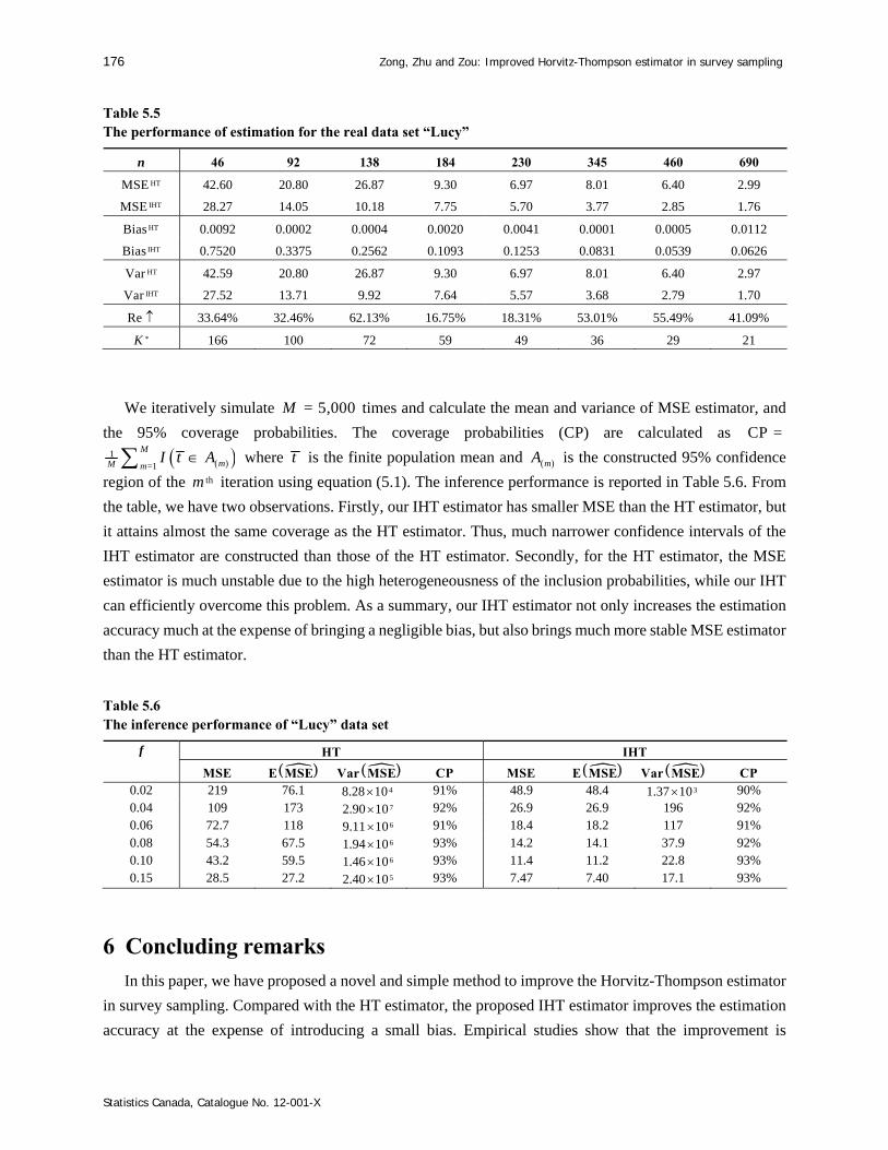
176 Zong, Zhu and Zou: Improved Horvitz-Thompson estimator in survey sampling
Statistics Canada, Catalogue No. 12-001-X
Table 5.5 The performance of estimation for the real data set “Lucy”
n 46 92 138 184 230 345 460 690
HTMSE 42.60 20.80 26.87 9.30 6.97 8.01 6.40 2.99
IHTMSE 28.27 14.05 10.18 7.75 5.70 3.77 2.85 1.76
HTBias 0.0092 0.0002 0.0004 0.0020 0.0041 0.0001 0.0005 0.0112
IHTBias 0.7520 0.3375 0.2562 0.1093 0.1253 0.0831 0.0539 0.0626
HTVar 42.59 20.80 26.87 9.30 6.97 8.01 6.40 2.97
IHTVar 27.52 13.71 9.92 7.64 5.57 3.68 2.79 1.70
Re 33.64% 32.46% 62.13% 16.75% 18.31% 53.01% 55.49% 41.09%
*K 166 100 72 59 49 36 29 21
We iteratively simulate = 5,000M times and calculate the mean and variance of MSE estimator, and
the 95% coverage probabilities. The coverage probabilities (CP) are calculated as CP =
1=1
M
mM mI t A where t is the finite population mean and mA is the constructed 95% confidence
region of the thm iteration using equation (5.1). The inference performance is reported in Table 5.6. From
the table, we have two observations. Firstly, our IHT estimator has smaller MSE than the HT estimator, but
it attains almost the same coverage as the HT estimator. Thus, much narrower confidence intervals of the
IHT estimator are constructed than those of the HT estimator. Secondly, for the HT estimator, the MSE
estimator is much unstable due to the high heterogeneousness of the inclusion probabilities, while our IHT
can efficiently overcome this problem. As a summary, our IHT estimator not only increases the estimation
accuracy much at the expense of bringing a negligible bias, but also brings much more stable MSE estimator
than the HT estimator.
Table 5.6 The inference performance of “Lucy” data set
f HT IHT
MSE E MSE Var MSE CP MSE E MSE Var MSE CP 0.02 219 76.1 8.28 410 91% 48.9 48.4 1.37 310 90% 0.04 109 173 2.90 710 92% 26.9 26.9 196 92% 0.06 72.7 118 9.11 610 91% 18.4 18.2 117 91% 0.08 54.3 67.5 1.94 610 93% 14.2 14.1 37.9 92% 0.10 43.2 59.5 1.46 610 93% 11.4 11.2 22.8 93% 0.15 28.5 27.2 2.40 510 93% 7.47 7.40 17.1 93%
6 Concluding remarks
In this paper, we have proposed a novel and simple method to improve the Horvitz-Thompson estimator
in survey sampling. Compared with the HT estimator, the proposed IHT estimator improves the estimation
accuracy at the expense of introducing a small bias. Empirical studies show that the improvement is
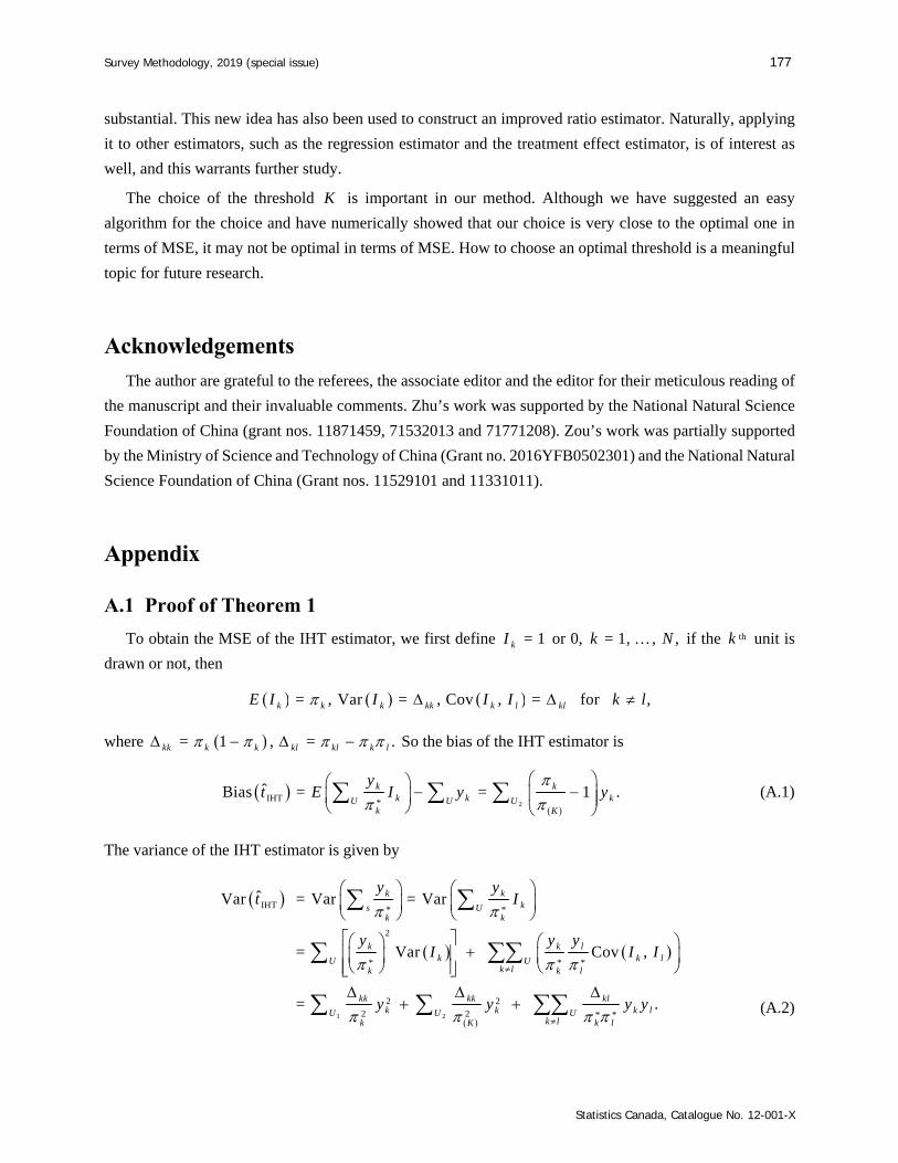
Survey Methodology, 2019 (special issue) 177
Statistics Canada, Catalogue No. 12-001-X
substantial. This new idea has also been used to construct an improved ratio estimator. Naturally, applying
it to other estimators, such as the regression estimator and the treatment effect estimator, is of interest as
well, and this warrants further study.
The choice of the threshold K is important in our method. Although we have suggested an easy
algorithm for the choice and have numerically showed that our choice is very close to the optimal one in
terms of MSE, it may not be optimal in terms of MSE. How to choose an optimal threshold is a meaningful
topic for future research.
Acknowledgements
The author are grateful to the referees, the associate editor and the editor for their meticulous reading of
the manuscript and their invaluable comments. Zhu’s work was supported by the National Natural Science
Foundation of China (grant nos. 11871459, 71532013 and 71771208). Zou’s work was partially supported
by the Ministry of Science and Technology of China (Grant no. 2016YFB0502301) and the National Natural
Science Foundation of China (Grant nos. 11529101 and 11331011).
Appendix A.1 Proof of Theorem 1
To obtain the MSE of the IHT estimator, we first define = 1kI or 0, = 1, , ,k N if the thk unit is
drawn or not, then
= , Var = , Cov , = for ,k k k kk k l klE I I I I k l
where = 1 , = .kk k k kl kl k l So the bias of the IHT estimator is
2IHT *
ˆBias = = 1 .k kk k kU U U
k K
yt E I y y
(A.1)
The variance of the IHT estimator is given by
1 2
IHT * *
2
* * *
2 22 2 * *
ˆVar = Var = Var
= Var Cov ,
= .
k kks U
k k
k k lk k lU U
k lk k l
kk kk klk k k lU U U
k lk k lK
y yt I
y y yI I I
y y y y
(A.2)
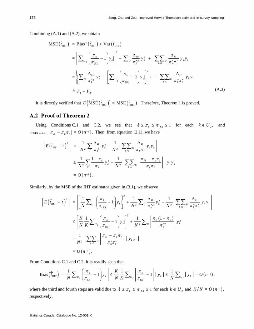
178 Zong, Zhu and Zou: Improved Horvitz-Thompson estimator in survey sampling
Statistics Canada, Catalogue No. 12-001-X
Combining (A.1) and (A.2), we obtain
2IHT IHT IHT
2
2*2 * *2
2
2*2 * *2
1 2
ˆ ˆ ˆMSE = Bias Var
= 1
= 1
.
k kk klk k k lU U U
k lk k lK
kk k klk k k lU U U
k lk k lK
t t t
y y y y
y y y y
F F
(A.3)
It is directly verified that IHT IHTˆ ˆMSE = MSE .E t t Therefore, Theorem 1 is proved.
A.2 Proof of Theorem 2
Using Conditions C.1 and C.2, we see that 1k K for each 2 ,k U and
2
1= .max k l U kl k l O n Then, from equation (2.1), we have
22
HT 22 2
2
2 2
1
1 1ˆ =
1 1 1
= .
kk klk l kU
U k lk k l
k kl k lk l kU
U k lk k l
E t t y y yN N
y y yN N
O n
Similarly, by the MSE of the IHT estimator given in (3.1), we observe
2
2
22
2IHT *22 2 * *
2
2*22
2 * *
1
1 1 1ˆ = 1
1 1 11
1
= .
k kk klk k k lU U U
k lk k lK
k k kk kU U
kK
kl k lk lU
k l k l
E t t y y y yN N N
Ky y
N K N
y yN
O n
From Conditions C.1 and C.2, it is readily seen that
2 2 2
1IHT
1 1 1ˆBias = 1 1 = ,k kk k kU U U
K K
Kt y y y O n
N N K N
where the third and fourth steps are valid due to 1k K for each 2k U and 1= ,K N O n
respectively.
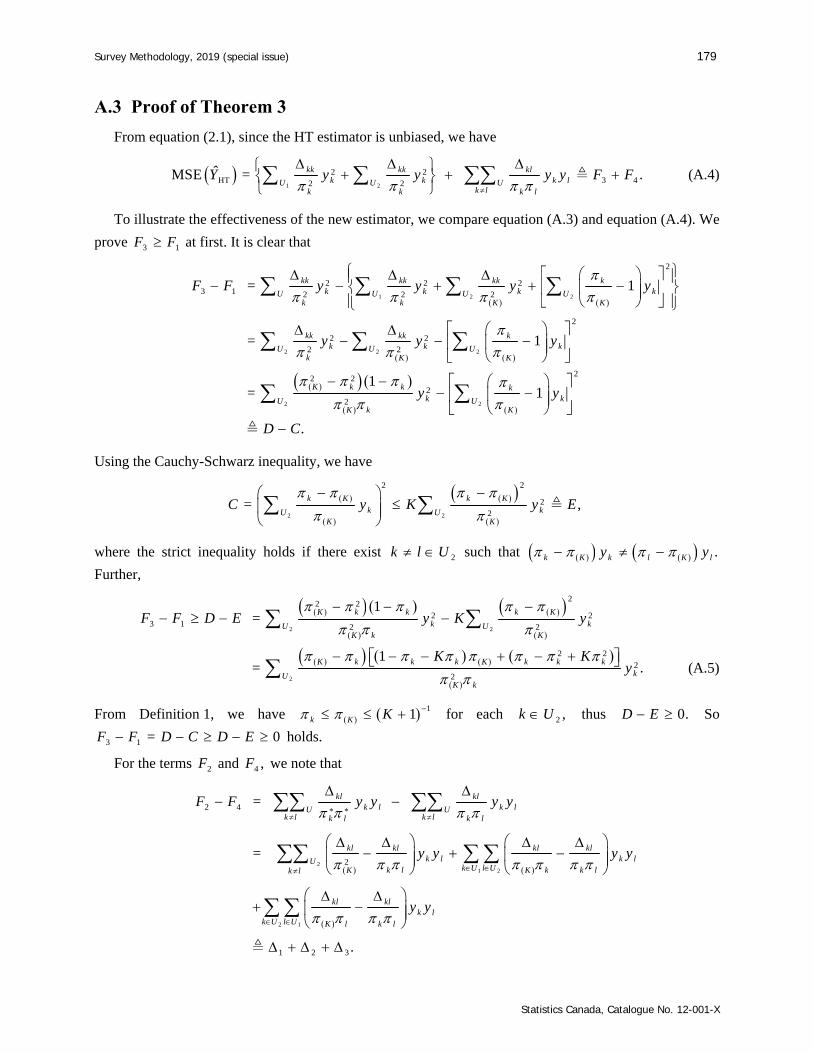
Survey Methodology, 2019 (special issue) 179
Statistics Canada, Catalogue No. 12-001-X
A.3 Proof of Theorem 3
From equation (2.1), since the HT estimator is unbiased, we have
1 2
2 2HT 3 42 2
ˆMSE = .kk kk klk k k lU U U
k lk k k l
Y y y y y F F
(A.4)
To illustrate the effectiveness of the new estimator, we compare equation (A.3) and equation (A.4). We
prove 3 1F F at first. It is clear that
1 2 2
2 2 2
2 2
2
2 2 23 1 2 2 2
2
2 22 2
22 2
22
= 1
= 1
1= 1
.
kk kk kk kk k k kU U U U
k k K K
kk kk kk k kU U U
k K K
k kK kk kU U
kK K
F F y y y y
y y y
y y
D C
Using the Cauchy-Schwarz inequality, we have
2 2
22
22
= ,k kK Kk kU U
K K
C y K y E
where the strict inequality holds if there exist 2k l U such that .k k l lK Ky y
Further,
2 2
2
22 2
2 23 1 2 2
2 22
2
1=
1= .
k k kK Kk kU U
kK K
k k k k k kK KkU
kK
F F D E y K y
K Ky
(A.5)
From Definition 1, we have 11k K K for each 2 ,k U thus 0.D E So
3 1 = 0F F D C D E holds.
For the terms 2F and 4 ,F we note that
21 2
2 1
2 4 * *
2
1 2 3
=
=
.
kl klk l k lU U
k l k lk l k l
kl kl kl klk l k lU
k U l Uk l k k lK Kk l
kl klk l
k U l U l k lK
F F y y y y
y y y y
y y
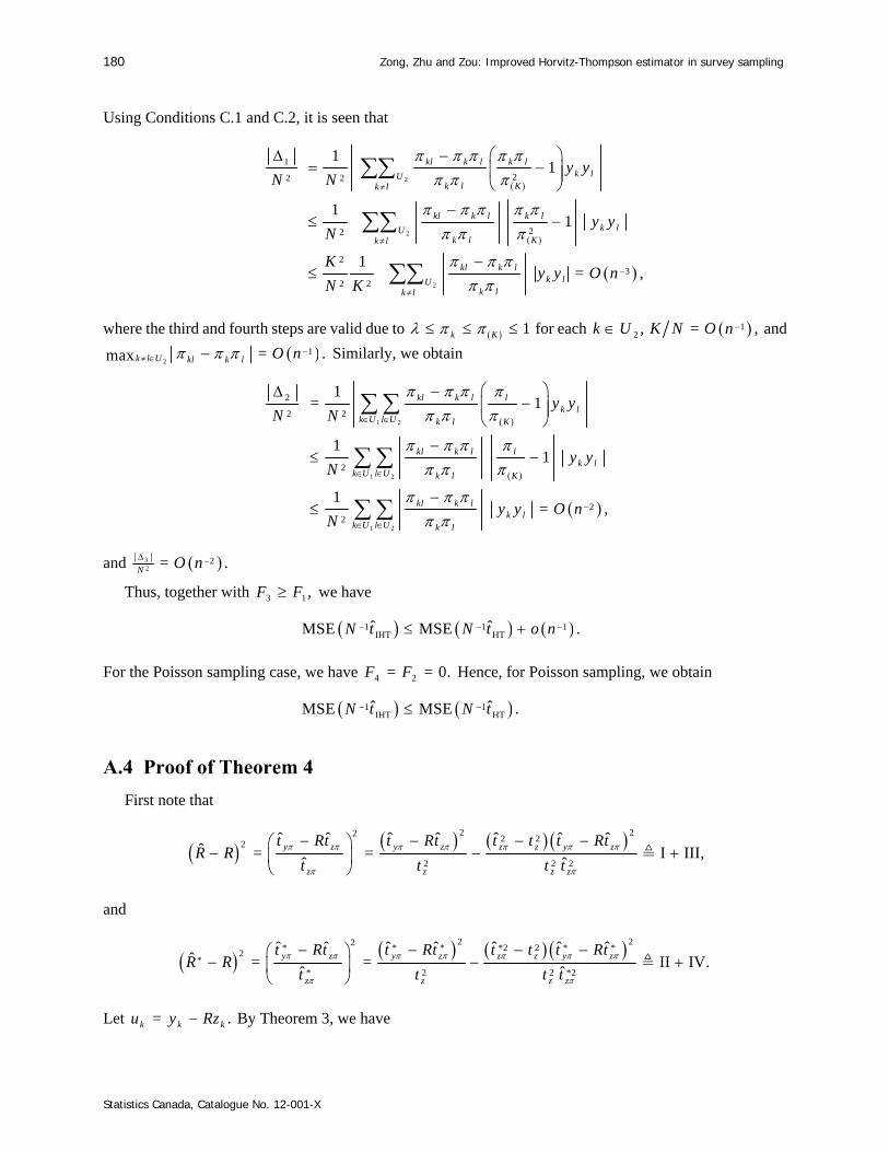
180 Zong, Zhu and Zou: Improved Horvitz-Thompson estimator in survey sampling
Statistics Canada, Catalogue No. 12-001-X
Using Conditions C.1 and C.2, it is seen that
2
2
2
1
22 2
22
23
2 2
11
11
1= ,
kl k l k lk lU
k l Kk l
kl k l k lk lU
k l Kk l
kl k lk lU
k lk l
y yN N
y yN
Ky y O n
N K
where the third and fourth steps are valid due to 1k K for each 2 ,k U 1= ,K N O n and
2
1= .max k l U kl k l O n Similarly, we obtain
1 2
1 2
1 2
2
2 2
2
22
1= 1
11
1= ,
kl k l lk l
k U l U k l K
kl k l lk l
k U l U k l K
kl k lk l
k U l U k l
y yN N
y yN
y y O nN
and 32
2= .N O n
Thus, together with 3 1 ,F F we have
1 1 1IHT HT
ˆ ˆMSE MSE .N t N t o n
For the Poisson sampling case, we have 4 2= = 0.F F Hence, for Poisson sampling, we obtain
1 1IHT HT
ˆ ˆMSE MSE .N t N t
A.4 Proof of Theorem 4
First note that
2 222 2
2
2 2 2
ˆ ˆ ˆ ˆ ˆ ˆ ˆˆ = = I III,
ˆ ˆy z y z z z y z
z z z z
t Rt t Rt t t t RtR R
t t t t
and
2 22* * * *2 2 * *
2*
* 2 2 *2
ˆ ˆ ˆ ˆ ˆ ˆ ˆˆ = = II IV.
ˆ ˆy z y z z z y z
z z z z
t Rt t Rt t t t RtR R
t t t t
Let = .k k ku y Rz By Theorem 3, we have

Survey Methodology, 2019 (special issue) 181
Statistics Canada, Catalogue No. 12-001-X
2 22 * 2 1ˆ ˆ .u u u uN E t t N E t t o n
Thus, for the terms I and II, we get
1I II .E E o n (A.6)
Now, we need to prove that the expectations of III and IV are negligible. Observe that,
2
2 2
2
2 2
*2
22*
*42
22*
ˆ ˆ ˆ ˆIII =
ˆ
ˆ ˆ ˆ ˆ
ˆ
ˆ ˆ ˆ
ˆ ˆ ˆ ,
z z z z y z
z z
z z z z y z
z z
zz z y z
z
zz z y z
z
t t t t t RtE E
t t
t t t t t RtE
t t
Z tE t t t Rt
t Z
Z tE t t E t Rt
t Z
where **= , = .max mink k
k k
z zn nk Uk UN NZ Z Similarly,
*
42* * *
22*
ˆ ˆ ˆIV ,zz z y z
z
Z tE E t t E t Rt
t Z
where * **
*= , = .max mink k
k k
z zn nk Uk UN NZ Z
Using Theorem 2 and Lemma 1, we see that 3 2(III) =E O n and 3 2IV = .E O n
Combining these and equation (A.6), we get
* 1ˆ ˆMSE MSE .R R o n
It implies that 1 * 1 1ˆ ˆMSE MSE .R RN Y N Y o n
A.5 Discussion on Condition C.4
Case 1: Simple random sampling without replacement
Under the simple random sampling without replacement, we have that = ni N for ,i U
11= n n
ij N N
for ,i j U
1 21 2= n n n
ijk N N N for ,i j k U and
1 2 31 2 3= n n n n
ijkl N N N N for .i j k l U It
follows that
12
2 1= = ,
1 2ijk ij k
n n N nO n
N N N
where the last equality is from Condition C.3. We also obtain
182 Zong, Zhu and Zou: Improved Horvitz-Thompson estimator in survey sampling
Statistics Canada, Catalogue No. 12-001-X
2 3
2 3 4
2
4 6 3
= 3 3
1 2 1= 3 6 3
1 2 3 1 2 1
= ,
ijkl ijk l ij k l i j k l
ijkl ijk l ijk l ij k l ij k l i j k l
n n n n N n n n N n n N
N N N N N N N N N
O n
where the last equality is from Condition C.3. Thus, Condition C.4 holds under the simple random sampling
without replacement.
Case 2: Poisson sampling
From the independence of Poisson sampling, =ij i j for ,i j U =ijk i j k for
,i j k U and =ijkl i j k l for .i j k l U Hence, = 0,ijk ij k and ijkl
4 6 3 = 0.ijk l ij k l i j k l It follows that Poisson sampling satisfies Condition C.4.
A.6 A lemma for proving Theorem 4
Lemma 1. For the HT estimator HTt and the IHT estimator ˆ ,IHTt under the Conditions C.1-C.4, we have
4 4
2 2ˆ ˆ= , = .HT IHTE t t O n and E t t O n
Proof. Noting that
HT
1 1ˆ = ,k kk k kU U
k
It t y J y
N N
we have
4
HT 4
4 3 2 2
4 4 4
2
4 4
1ˆ =
1 4 3=
6 1
I II III IV V.
k k l l i i j jk l i j
k k k k l l k k l lU k l k l
i i k k l l i i j j k k l li k l i j k l
t t J y J y J y J yN
J y J y J y J y J yN N N
J y J y J y J y J y J y J yN N
For the first term I, using 1k and 1k kI for any ,k U we get
4 4
4 4 24 4 4
1 1 1= = = ( ).k k
k k k kU U Uk k
y yE I E J y E I O n
N N N
For the terms II and III, we have

Survey Methodology, 2019 (special issue) 183
Statistics Canada, Catalogue No. 12-001-X
3 333 3 3 4
1 1 1 1( ) = ,k l k k l l k k l l
k l k l k l
E J J E I I E I I
and
2 22 22 2 2 2 4
1 1 1= .k l k k l l
k l k l
E J J E I I
Thus, 2II =E O n and 2(III) = .E O n For the fourth term IV, we have that
222
22
1
1=
1= 1 2
= ,
i k l i i k k l li k l
i ikl ik l k il i l i kl k li k l
E J J J E I I I
O n
where the last step is from Conditions C.1 and C.4. It implies that 2IV = .E O n For the last term V,
we have that
4
4
2
1
4 6 31=
= ,
i i j j k k l li j k l
ijkl ijk l ij k l i j k li j k l
i j k l i j k l
E J y J y J y J yN
y y y yN
O n
where the last step is from Conditions C.1 and C.4. Thus, 4
2HT
ˆ =E t t O n holds.
Next we shall prove 4
2IHT
ˆ = .E t t O n Noting that
* *
IHT * * *
1 1 1ˆ = = ,k k k k k kk k k
U U Uk k k
I It t y y y A
N N N
we have
4 4 4 3 2 2 3 4
IHTˆ = = 4 6 4 .E t t E A E A E A E A E A (A.7)
Similar as the proofs of the result 4
2HT
ˆ = ,E t t O n using * 1,k it is easy to obtain
4
4 2*
1= = .k k
kU k
IE A E y O n
N
(A.8)
From equation (A.8), we have that 2 1=E A O n and 3 3 2= .E A O n Meanwhile = 0E A and
2
* *1
* *
1 1= = = .k k k k
k kU Uk k
Ky y O n
N N K
Therefore, from equation (A.7), we prove that 4
2IHT
ˆ = .E t t O n

184 Zong, Zhu and Zou: Improved Horvitz-Thompson estimator in survey sampling
Statistics Canada, Catalogue No. 12-001-X
References Breidt, F.J., and Opsomer, J.D. (2000). Local polynomial regression estimators in survey sampling. Annals
of Statistics, 28, 1026-1053. Cardot, H., and Josserand, E. (2011). Horvitz-thompson estimators for functional data: Asymptotic
confidence bands and optimal allocation for stratified sampling. Biometrika, 98, 107-118. Gutierrez, H.A. (2009). Estrategias de muestreo: Diseno de encuestas y estimacion de parametros. Editorial
Universidad Santo Tomas. Hansen, M., and Hurwitz, W. (1943). On the theorey of sampling from finite populations. Annals of
Mathematical Statistics, 14, 333-362. Hoerl, A., and Kennard, R. (1970). Ridge regression: Biased estimation for nonorthogonal problems.
Technometrics, 12, 55-67. Horvitz, D., and Thompson, D. (1952). A generalization of sampling without replacement from a finite
universe. Journal of the American Statistical Association, 47, 663-685. Rosenbaum, P. (2002). Observational Studies. New York: Springer. Tibshirani, R. (1996). Regression shrikage and selection via the lasso. Journal of the Royal Statistical
Society, Series B, 58, 267-288.

GUIDELINES FOR MANUSCRIPTS
Authors are invited to submit their articles through the Survey Methodology hub on the ScholarOne Manuscripts website (https://mc04.manuscriptcentral.com/surveymeth). Before submitting the article, please examine a recent issue of Survey Methodology (Vol. 39, No. 1 and onward) as a guide and note particularly the points below. Articles must be submitted in machine-readable form, preferably in Word with MathType for the mathematical expressions. A pdf or paper copy may be required for formulas and figures. 1. Layout 1.1 Documents should be typed entirely double spaced with margins of at least 1½ inches on all sides. 1.2 The documents should be divided into numbered sections with suitable verbal titles. 1.3 The name (fully spelled out) and address of each author should be given as a footnote on the first page of the
manuscript. 1.4 Acknowledgements should appear at the end of the text. 1.5 Any appendix should be placed after the acknowledgements but before the list of references. 2. Abstract
The manuscript should begin with an abstract consisting of one paragraph followed by three to six key words. Avoid mathematical expressions in the abstract.
3. Style 3.1 Avoid footnotes, abbreviations, and acronyms. 3.2 Mathematical symbols will be italicized unless specified otherwise except for functional symbols such as “exp(·)” and
“log(·)”, etc. 3.3 Short formulae should be left in the text but everything in the text should fit in single spacing. Long and important
equations should be separated from the text and numbered with arabic numerals on the right if they are to be referred to later. Use a two-level numbering system based on the section of the paper. For example, equation (4.2) is the second important equation in section 4.
3.4 Write fractions in the text using a solidus. 3.5 Distinguish between ambiguous characters, (e.g., w, ; o, O, 0; l, 1). 3.6 If possible, avoid using bold characters in formulae. 4. Figures and Tables 4.1 All figures and tables should be numbered with arabic numerals, with titles that are as self explanatory as possible, at
the bottom for figures and at the top for tables. Use a two-level numbering system based on the section of the paper. For example, table 3.1 is the first table in section 3.
4.2 A detailed textual description of figures may be required for accessibility purposes if the message conveyed by the image is not sufficiently explained in the text.
5. References 5.1 References in the text should be cited with authors’ names and the date of publication. If part of a reference is cited,
indicate after the reference, e.g., Cochran (1977, page 164). 5.2 The list of references at the end of the manuscript should be arranged alphabetically and for the same author
chronologically. Distinguish publications of the same author in the same year by attaching a, b, c to the year of publication. Journal titles should not be abbreviated. Follow the same format used in recent issues.
6. Short Notes 6.1 Documents submitted for the short notes section must have a maximum of 3,000 words.