Surveillance of the covariance matrix based on the properties of the singular Wishart distribution

Computational Statistics and Data Analysis 53 (2009) 3372–3385

Contents lists available at ScienceDirect

Computational Statistics and Data Analysis

journal homepage: www.elsevier.com/locate/csda

Surveillance of the covariance matrix based on the properties of thesingular Wishart distributionOlha Bodnar a, Taras Bodnar a, Yarema Okhrin b,∗a Department of Statistics, European University Viadrina, PO Box 1786, D-15207 Frankfurt (Oder), Germanyb Department of Economics, University of Bern, CH-3012 Bern, Switzerland

a r t i c l e i n f o

Article history:Received 12 November 2007Received in revised form 11 February 2009Accepted 11 February 2009Available online 6 March 2009

a b s t r a c t

A methodology which allows applying the standard monitoring techniques for the meanbehaviour of Gaussian processes in the detection of shifts in the covariance matrix isdeveloped. Moreover, the proposed methodology allows the use of an estimator of thecovariance matrix based on a single observation. An extensive simulation study revealsthe advantages of the considered approach.

© 2009 Elsevier B.V. All rights reserved.

1. Introduction

Statistical process control methods play an important role in quality improvement. They have been widely applied inEngineering for a long time. The aim is to detect a structural change in the process of interest as soon as possible afterits occurrence. However, this problem setting is also important in other fields and recently several papers discussed theapplications of sequential procedures in Economics,Medicine, Chemistry, and Finance (see Frisén (1992), Sonesson and Bock(2003), Lawson and Kleinman (2005), Schipper and Schmid (2001), Andersson et al. (2004), Schmid and Tzotchev (2004),Bodnar (2007) and Messaoud et al. (2008) among others). This leads to more advanced models with time dependent andmultivariate processes.Themain tools of statistical process control are control charts. A control chart is characterized by a control statistic which

is updated by using current information at each timepoint.When the control statistic exceeds the preselected value the chartsignals an alarm, suggesting that a change in the parameters of the underlying process has occurred. The first control chartfor the mean of an independent Gaussian process was proposed by Shewhart (1931). Later on, Page (1954) and Roberts(1959) derived control charts with memory, the so-called CUSUM and EWMA control charts respectively.The extension of the univariate control charts to the multivariate case is not trivial and can be implemented in

many alternative ways. The first multivariate control scheme for the mean was proposed by Hotelling (1947), which isa multivariate generalization of the univariate scheme of Shewhart (1931). The EWMA chart was extended by Lowryet al. (1992). Since the univariate CUSUM control scheme was derived from the sequential probability ratio test (SPRT)its generalization to the multivariate case is not straightforward. In the multivariate case the CUSUM chart depends on thesize and direction of the expected shift. For that reason several authors proposed schemes for the mean which exclusivelydepend on themagnitude of the expected shift like, Crosier (1988), Pignatiello and Runger (1990) andNgai and Zhang (2001).Note that all the abovementioned charts are developed to detect shifts in themean behaviour of the process. Application

to other areas makes the monitoring of the variance or the covariance matrix increasingly important. In general we canapply the techniques of the mean charts to different volatility measures (Okhrin and Schmid, 2008a,b). Usually squared

∗ Corresponding address: Department of Economics, University of Bern, Schanzeneckstrasse 1, CH-3012 Bern, Switzerland. Tel.: +41 31 631 4792;fax: +41 31 631 3783.E-mail address: [email protected] (Y. Okhrin).

0167-9473/$ – see front matter© 2009 Elsevier B.V. All rights reserved.doi:10.1016/j.csda.2009.02.020

http://www.elsevier.com/locate/csda

http://www.elsevier.com/locate/csda

mailto:[email protected]

http://dx.doi.org/10.1016/j.csda.2009.02.020

O. Bodnar et al. / Computational Statistics and Data Analysis 53 (2009) 3372–3385 3373

observations, their logarithms or other transformations are used. This leads, however, to non-standard distributions of thecontrol statistics and substantially complicates the monitoring process. This fact is even more critical in the multivariatecase due to a large number of components in the covariance matrix. Moreover, note that the discussion is most of the timerestricted to EWMA schemes (see Yeh et al. (2005), Śliwa and Schmid (2005), Reynolds and Cho (2006) and Huwang et al.(2007)). The derivation of CUSUM charts for covariance matrices is technically difficult. For this reason, the few papersdealing with this type of charts translate the univariate schemes for the mean into multivariate schemes for variancemeasures (see Hawkins (1981, 1991)). Chan and Zhang (2001) suggested a CUSUM-type control chart for the covariancematrix of independent observations based on the projection pursuit method.In this paperwe introduce a new technique,which allows us to apply the standard EWMAor CUSUMcontrol charts for the

mean directly tomonitor the covariancematrix of a Gaussian vector. Moreover, themethod can be applied to the estimatorsof the covariancematrix based on a single recent observation. The idea of the approach is to transform the variance estimatorto a set of Gaussian vectors. This can be done by using properties of theWishart and singularWishart distributions. The shiftin the variance of the original process would cause a shift in the mean of the transformed quantities. This implies thatmonitoring the variance of the original process is equivalent to monitoring the mean of the Gaussian vectors. For the latterproblem the classical control charts can be applied.The rest of the paper is organized as follows. In the next section the change point model is presented. Then we establish

the necessary properties of the singular Wishart distribution. Furthermore, we review the multivariate control charts usedfor monitoring. The simulation study in Section 4 compares the modified charts for the covariance matrix with the chartsbased on the transformed Gaussian quantities introduced in this paper. The proofs are given in the Appendices A and B.

2. Models for the target and the observed processes

In order to define the control problem we distinguish the target process and the observed process. The target process isthe process that fulfills the quality requirements. Usually, it depends on some parameters, that can be set to correspondingtarget values (industry) or estimated using previous data (economics, finance). The observed process is the actual processthat we observe in practice. Our task is to decide if the observed and the target processes coincide.We denote the target process by {Yt}. It is assumed that Y1, . . . , Yn are identical and independently normally distributed

withYi ∼ Np(µ1,61), where the covariancematrix can bewritten as61 = D1R1D1. ThematricesD1 andR1 are the diagonalmatrix of standard variances and the correlation matrix, respectively. All parameters of the target process are assumed tobe known. In practice, however, especially in economic applications, the parameters of the target process are estimated.This causes an additional estimation risk. The impact of parameter uncertainty in the target process is beyond the scope ofour paper. The interested reader should refer to Kramer and Schmid (2000) and Albers and Kallenberg (2004) where suchproblems are discussed. Without loss of generality we assume that µ1 = 0.We denote the observed process by {Xt}. To model the observed process we apply the change point framework, i.e.

Xt ∼{Np(0,D1R1D1), t < qNp(0,D∆R∆D∆), t ≥ q , (1)

where D∆ and R∆ are the diagonal matrix of standard variances and the correlation matrix after the change. D∆, R∆, andq ∈ IN are unknown quantities. In the case q < ∞ we say that there is a change at the time point q. In the case of nochange the target process coincides with the observed process. We say that the observed process is in control, i.e. Xt = Yt .The in-control covariance matrix61 is called the target covariance matrix. If the change occurs the process is said to be outof control. The change can be in the variances, in the correlations or in both quantities simultaneously. For changes in thevariance we assume that D∆ = 1D1 with a diagonal matrix of shifts 1, for changes in the correlations we set R∆ = 1R1where 1 is a positive definite correlation matrix. For changes in both quantities we assume that 6∆ = 161 where 1 isa symmetric positive definite matrix. If 1 is an identity matrix we have no shifts. Note that Xt = Yt for t ≤ 0, i.e. bothprocesses are the same up to time point q − 1. In the theoretical statements of Section 3 we assume that the shift occursjust before we collect the first sample, i.e. q = 1. In the simulation study in Section 4 we consider the maximum averagedelay as a performance measure of control carts. Therefore, here the shift is assumed to occur at an arbitrary time point q(see (20) and (21)).

3. Control charts for the covariance matrix

As an estimator of the covariance matrix we use the point estimator based on a single observation, i.e. at time point tthe covariance matrix is estimated by Vt = XtX′t . The matrix Vt follows a singular Wishart distributed Vt ∼ Wp(1,6) (see,e.g. Srivastava (2003)), where6 = 61 if the process is in control and6 = 6∆ if the process is out of control. Its rank is equalto one with probability one in both cases. It is not new to exploit the unbiased point estimator Vt for monitoring purposes.Yeh et al. (2005) used Vt to update the matrix variate EWMA recursion.However, the standard control schemes cannot be directly applied to the point estimator Vt . For the EWMA chart, the

variance of the control statistic has to be computed and this is a nontrivial task. Moreover, because the distribution of thecontrol statistic is not symmetric, the two-sided EWMA chart for the variance depends on two critical values (see, e.g. Chan

3374 O. Bodnar et al. / Computational Statistics and Data Analysis 53 (2009) 3372–3385

and Zhang (2001)). This generates additional computational difficulties. In this paper we use the properties of the singularWishart distribution to transform Vt to a set of Gaussian vectors. Then the mean charts can be immediately applied tomonitoring the shifts in the variance.The important distributional properties of the singular Wishart distribution are summarized in Theorem 1. Let σ1;ii

denotes the (i, i)th element of the matrix 61, i = 1, . . . , p. By 61;21,i we denote the ith column of the matrix 61 withoutσ1;ii. Let 61;22,i denote a quadratic matrix of order p− 1, which is obtained from the matrix 61 by deleting the ith row andthe ith column. Let61;22·1,i = 61;22,i−61;21,i6

′

1;21,i/σ1;ii. In the sameway we define vt;ii, Vt;21,i, Vt;22,i, Vt;22·1,i, σ∆;ii,6∆;21,i,6∆;22,i, and 6∆;22·1,i by splitting Vt and 6∆ respectively.

Theorem 1. Let Y1, . . . , Yn be an identically independently distributed Gaussian process with Yi ∼ Np(0,61). We assume thatthe observed process {Xt} is defined according to the model (1). Then

(a) in the in-control state

ηi,t = 6−1/21;22·1,i(Vt;21,i/vt;ii − 61;21,i/σ1;ii)v

1/2t;ii ∼ Np−1(0p−1, Ip−1)

and is independent of vt;ii;(b) in the out-of-control state

E(ηi,t) = 6−1/21;22·1,i�iσ

1/21;ii

√2√π,

Var(ηi,t) = 6−1/21;22·1,i

(6∆;22·1,i + �iσ1;ii(1− 2π−1)�′i

)6−1/21;22·1,i,

where�i = 6∆;21,i/σ∆;ii − 61;21,i/σ1;ii.Moreover, the process {ηi,t} is independent in time both in the in-control and in the out-of-control states.

For the proof of the first part of the theorem we refer to Bodnar and Okhrin (2008). The proof of the second part is given inthe Appendix A.In the first part of Theorem 1 it is shown that ηi,t follows standard normal distribution for each i and t . Furthermore, it

holds that ηi,t1 and ηi,t2 are independent as long as Xt1 and Xt2 are independent. In the out-of-control state we observe achange in the mean vector of ηi,t if �i 6= 0. This is, however, not the case if we consider the change point model as in (1).Thus, the transformation ηi,t translates the shift in the covariance matrix into a shift in the mean. Note that the covariancematrix and the distribution of ηi,t change in the out-of-control state too.

Remark 1. The distribution of ηi,t is no longer multivariate normal if we have a change in the mean vector of Yt , i.e. Xt =µ+Yt . To show this point, we assume for simplicity, that there is only a change in themean vector and the covariancematrixremains the same in the out-of-control state. Then, the density of η1;t = 6

−1/222·1 (Vt;21/vt;11 − 621/σ11)v

1/2t;11 is given by

fη1(z) =π−k/22−(k−2)/2

σ1/211

∫∞

0exp

(−12(σ−111 t

2+ z′z)

)× cosh(

√µ′µ

√[t, t6′21/σ11 + (6

1/222·1z)′]6

−2[t, t621/σ11 + 6

1/222·1z]′) dt,

where cosh(.) denotes the hyperbolic cosine function. The derivation of the density function is given in the Appendix B.A similar result holds for other vectors ηi,t . Hence, the control statistics, that are constructed using ηi,t will be sensitive

to both shifts in the covariance matrix and shifts in the mean. In the multivariate setup we rarely have a justified reason toexpect shifts only in the mean or only in the covariance matrix. This makes the diagnostic of the alarms generated by theschemes based on ηi,t particularly difficult. Nevertheless, note that a vastmajority of the control charts for the variability aresensitive to the mean shifts too. This argument is supported by the results of the simulation study (see Section 4). The onlyexception is the MEWMV chart of Huwang et al. (2007). The chart successfully eliminates the impact of potential shifts inthemean by subtracting from the process the EWMA-type estimator of themean. Unfortunately, due to technical difficultieswe were unable to generalize the above theoretical results to the setup of Huwang et al. (2007), we provide some furtherdiscussion of this procedure in Section 4. Furthermore, note that using the developed methodology for detecting shifts onlyin the mean is not very promising, since there are numerous well established and much simpler charts developed for thistype of changes. Therefore, in this paper we focus only on the shifts in the covariance matrix.

The normality, time independency and the shift in the mean caused by the shift in the covariance matrix allow us to usethe standard multivariate EWMA and CUSUM control schemes of Crosier (1988), Pignatiello and Runger (1990), Lowry et al.(1992), and Ngai and Zhang (2001) to monitor changes in the means of the processes {ηi,t}. Note that we have p vectors ηi,tand each of them should be monitored. To cope with this problem we follow the approach of Woodall and Ncube (1985).The simultaneous use of univariate control charts for each i is considered to be a single joint control chart. This control chartgives an alarm if at least one of the individual charts signals a shift. The Sections 3.2 and 3.3 contain technical details of theimplementation of these charts.


As benchmarkwe consider the control chartswhichmonitor the covariances of the process directly. A detailed discussionof the EWMA-type charts of Yeh et al. (2005), Śliwa and Schmid (2005), Reynolds and Cho (2006) and Huwang et al. (2007)as well as of the CUSUM-type chart of Chan and Zhang (2001) are given in Section 3.4. There are a few charts dealing withCUSUM procedures for the covariance matrices. This is due to the fact that the CUSUM schemes are either derived fromthe sequential probability ratio test or simply mimic the univariate charts. In the former case no theoretical results areavailable for monitoring the covariances. In the latter case, however, the problem of the direction of the shift is crucial.These drawbacks hinder the application of multivariate CUSUM charts to covariance monitoring. Moreover, since the chartof Yeh et al. (2005) outperforms the CUSUM scheme of Hawkins (1991), we concentrate exclusively on EWMA benchmarkswith the only exception of the PPCUSUMv chart of Reynolds and Cho (2006).

3.1. T 2 control chart

The first multivariate control chart for independent observation was derived by Hotelling (1947). Here this controlscheme can be applied to the processes {ηi,t}. The control statistic is given by

T 2t = max1≤i≤p{T 2i,t}, where T 2i,t = η′i,tηi,t . (2)

Note that the individual control statistics T 2i,t are χ2-distributed with p degrees of freedom in the in-control state. However,

the distribution of the T 2t statistic is much more complicated. Unfortunately this classical control chart provided the worstresults in the simulation study, and, therefore, we skip it from further discussion.

3.2. CUSUM control charts

Crosier (1988) considers a generalization of the univariate CUSUM chart of Crosier (1986) to the multivariate setting. Inthis approach the univariate quantities are replaced with vectors. Moreover, instead of shrinking against zero by a multipleof the standard deviation, the multivariate control statistic is scaled along some predetermined direction. Here we apply

the CUSUM scheme of Crosier (1988) to the processes {ηi,t}. Let ‖a‖ =√a21 + a

22 + · · · + a2p be the Euclidean norm of the

p-dimensional vector a. Further let Ci,t = ‖Si,t−1 + ηi,t‖, where

Si,t =

0 if Ci,t ≤ k

(Si,t−1 + ηi,t)

(1−

kCi,t

)if Ci,t > k

(3)

for t ≥ 1 with Si,0 = 0. k > 0 plays the role of a reference value.MCUSUMi,t is the length of the vector Si,t defined by

MCUSUMi,t = (S′i,tSi,t)1/2= max{0, Ci,t − k}. (4)

The individual control chart signals an alarm ifMCUSUMi,t exceeds some preselected critical value. To have a unique criticalvalue of the joint control chart we define the control statistic of the joint scheme by

MCUSUMt = max1≤i≤p{MCUSUMi,t}. (5)

The scheme gives an out-of-control signal if MCUSUMt exceeds a preselected control limit h. The value of h is determinedwithin a simulation study.Pignatiello and Runger (1990) proposed two types of multivariate CUSUM charts, namely MC1 and MC2. Let Si;m,l =∑lj=m+1 ηi,t for l,m ≥ 0. The control statistic of the individual control charts is defined as

MC1i,t = max{‖Si;t−ni,t ,t‖ − kni,t , 0}, t ≥ 1, (6)

where

ni,t ={ni,t−1 + 1 ifMC1i,t−1 > 01 ifMC1i,t−1 = 0.

(7)

The decision rule of the joint MC1 scheme is constructed by defining theMC1 statistic as follows

MC1t = max1≤i≤p{MC1i,t}. (8)

The chart signals an alarm ifMC1t > h for some fixed critical value h. The second chart considered by Pignatiello and Runger(1990) is based on

MC2t = max1≤i≤p{MC2i,t}, (9)


where

MC2i,t = max{0,MC2i,t−1 + D2i,t − p− k}, t ≥ 1 (10)

with D2i,t = η′i,tηi,t andMC2i,0 = 0. Similarly as for the first chart we observe a signal ifMC2t > h.Using the projection pursuit approach Ngai and Zhang (2001) derived the PPCUSUM chart. Applying this approach to the

processes {ηi,t}we obtain the following CUSUM statistic

PPCUSUMt = max1≤i≤p{PPCUSUMi,t} (11)

with

PPCUSUMi,t = max{0, ‖Si;t−1,t‖ − k, ‖Si;t−2,t‖ − 2k, . . . , ‖Si;0,t‖ − tk} (12)

for t ≥ 1 with Si;t−v,t defined above. The control scheme gives an alarm as soon as PPCUSUMt > h.

3.3. MEWMA control charts

An alternative class of charts constitute the EWMA schemes. Lowry et al. (1992) proposed a control chart based on themultivariate EWMA recursion. As in the univariate case we define Zi,t = rηi,t + (1− r)Zi,t−1 with Zi,0 = 0. We distinguishbetween the use of the exact or of the asymptotic variance of Zi,t . The control statistic of the individual charts is thendefined by

Qi,t =2− r

r(1− (1− r)2t)Z′i,tZi,t and Qai,t =

2− rr

Z′i,tZi,t (13)

respectively. The joint MEWMA statistic is then given by

MEWMAt = max1≤i≤p{Qi,t} and MEWMAat = max

1≤i≤p{Qai,t}. (14)

The second approach of deriving the EWMA chart is based on calculating the Mahalanobis distance of ηi,t and thenapplying the EWMA recursion to this distance. The individual control chart in this case is given by

QMi,t = rD2i,t + (1− r)QMi,t with QMi,0 = p− 1. (15)

The EWMA chart based on the Mahalanobis distance signals an alarm as soon as the control statistic

MEWMAMt = max1≤i≤p{QMi,t} (16)

exceeds the preselected control limit.

Remark 2. Note that the design of the suggested control charts can be further simplified. Let Xt = 6−1/21 Xt . Then it holds

that Vt = Xt X′

t isWp(1, 0) in the in-control state andWp(1,6−1/21 6∆6

−1/21 ) in the out-of-control state. Furthermore, from

Theorem 1 we obtain that

ηi,t = Vt;21,i/v1/2t;ii = (−1)

1{Xi<0}(X1, . . . , Xi−1, Xi+1, . . . , Xp)′

follows the standard normal distribution, where the symbol 1A denotes the indicator function of the set A. Using ηi,t insteadof ηi,t in the definition of the control charts simplifies the calculation of the control statistics. Later on, we refer to the controlschemes based on ηi,t as standardized control charts.

3.4. Benchmark charts

In this section we review the control charts which we use as benchmarks in the simulation study. Śliwa and Schmid(2005) derived the EWMAcontrol charts for detecting changes in the covariancematrix of theGaussian vector autoregressive(VARMA) process. The Gaussian processwith independent realizations is a special case of the VARMAprocess. Consequently,we can apply their approach to monitor the covariance matrix of Yt .Let

τt =(X1,tX1,t , X1,tX2,t , . . . , Xp−1,tXp,t , Xp,tXp,t

)′= vech(Vt).

It holds that

µτ = E(vech(Vt)) ={vech(61), t < qvech(6∆), t ≥ q.


Moreover, Śliwa and Schmid (2005) provided the expression for the in-control covariance matrix of τt , which we denote byVar1(τt) = 6τ . It is used in the computation of the control statistic.The multivariate EWMA chart is given by

MEWMAot = (Zt − µτ )′Cov1(Zt)−1(Zt − µτ ), (17)

where Zt = rτt + (1− r)Zt−1 with Z0 = µτ .For the EWMA chart based on the Mahalanobis distance we consider

D2t = (τt − µτ )′6−1τ (τt − µτ ).

The control statistic is given by

MEWMAMot = rD2t + (1− r)MEWMAMot−1 (18)

withMEWMAMo0 = p(p+ 1)/2.Yeh et al. (2005) applied the EWMA recursion to construct a weighted estimator of the covariance matrix of the normal

distribution. The estimator is given by

St = rXtX′t + (1− r)St−1, (19)

where r ∈ (0, 1]. Let S1;t and S2;t denote the stacked diagonal and nondiagonal elements of St respectively, i.e.

S1;t = (s11;t , . . . , spp;t)′, S2;t = (s12;t , s13;t , . . . , sij;t , , . . . , sp−1p;t)′.

The deviations from the target value are squared and cumulated as follows

D1;t =p∑i=1

(sii;t − σ(0)ii )

2, D2;t =∑

1=i<j=p

(sij;t − σ(0)ij )

2.

The control statistic in Yeh et al. (2005) is then given by the maximum of the standardized cumulated shift in the variancesand in the covariances

MaxDt = max{D1;t − µD1

σD1,D2;t − µD2

σD2

},

where the asymptotic moments µD1 , µD2 , σD1 and σD2 can be found in the original paper.Huwang et al. (2007) suggest another EWMA chart, which detects shifts in the covariance matrix bymonitoring its trace.

The control statistic of this chart is given by

MEWMSt =tr(St)− µtr

σtr,

where

µtr = p and σ 2tr = 2p

((1− r)2(t−1) +

t∑i=2

r2(1− r)2(t−i)).

The quantity St is defined as in (19) and tr(·) denotes the trace of the matrix. The control chart signals an alarm ifMEWMStexceeds a preselected control limit.While monitoring the variance of the process it is usually assumed that the mean stays constant. In practice it is difficult

to verify this assumption. Huwang et al. (2007) suggest a chart for the covariance matrix which is insensitive to the shifts inthe mean vector. The control statistics is given by

MEWMVt = r(Xt − Yt)(Xt − Yt)′ + (1− r)MEWMVt−1,

with Yt = rXt + (1 − r)Yt−1 and MEWMV0 = (X1 − Y1)(X1 − Y1)′ and Y0 = 0. We can select either equal or differentsmoothing parameters in both the recursions. In the simulation study we set r = 0.2 and optimize the chart with respect tor . This makes the chart comparable with other charts, which depend on a single parameter too. The choice of r is in line withthe results of the simulation study by Huwang et al. (2007), where the best results are obtained for r = 0.2. The MEWMVchart gives an alarm ifMEWMVt/

√Var(MEWMVt) exceeds some preselected level.

Reynolds and Cho (2006) suggest four control schemes for detecting changes in the covariance matrix that are based onthe EWMA recursion. For the first two we define

EZi,t = (1− r)EZi,t−1 + rX2i,t i = 1, . . . , p


with EZi;0 = 1. Let6(2)1 denote the matrix with the elements that are squares of the corresponding elements of61. Then the

statistics of the control charts are expressed as

M1Z2t =2− r2r

(EZ1,t − 1, . . . , EZp,t − 1)(6(2)1

)−1(EZ1,t − 1, . . . , EZp,t − 1)′,

M2Z2t =2− r2r

(EZ1,t , . . . , EZp,t)(6(2)1

)−1(EZ1,t , . . . , EZp,t)′.

These charts are computed as Mahalanobis distances of the EWMA recursions applied to the squared or demeaned squaredobservations.The other two control charts of Reynolds and Cho (2006) are based on the squared deviations from the target of the

regression-adjusted variables (see Hawkins (1991), Hawkins (1993)). The vector of the regression-adjusted variables isgiven by

At = (diag6−11 )−1/26−11 Xt ,

where diag6−11 is a diagonal matrix with the same diagonal elements as 6−11 . It holds E(At) = 0, 6A,∆ =

(diag6−11 )−1/26−11 D∆R∆D∆6−11 (diag6

−11 )−1/2 in the out-of-control state, and 6A,1 = (diag6−11 )

−1/26−11 (diag6−11 )−1/2 in

the in-control state. Then the control statistics are defined by

M1A2t =2− r2r

(EA1,t − 1, . . . , EAp,t − 1)(6(2)A,1

)−1(EA1,t − 1, . . . , EAp,t − 1)′,

M2A2t =2− r2r

(EA1,t , . . . , EAp,t)(6(2)A,1

)−1(EA1,t , . . . , EAp,t)′,

where EAi,t is defined similarly to EZi,t by replacing Xt with At .Using the projection pursuit method, Chan and Zhang (2001) derived the PPCUSUMv control chart. Let λuji and λ

lji be the

largest and the smallest eigenvalues of XjX′j + · · · + XiX′i . We define

SUji = λuji − (i− j+ 1)ku and SLji = λlji − (i− j+ 1)kl.

Then the PPCUSUMv chart gives an out-of-control message as soon as

SUi > hu or SLi < hl,

where

SUi = max{0, SU1i, . . . , SUii} and SLi = min{0, SL1i, . . . , SLii}.

To simplify the calculation of the control statistic, Chan and Zhang (2001) suggested the use of ku = 1.5, kl = 0.5, andhl = hu = h.

4. Simulation study

The goal of this section is to compare the performance of the control charts derived in the previous section. To assess theperformance it is necessary to define suitable performance measures. All the relevant ones are based on the run length ofthe control chart which is defined as

tA = inf {t ∈ N : Ct ≥ c},

where Ct denotes the control statistic and c denotes the control limit. The run length is equal to the number of observationstaken until the first alarm of the chart.The most popular performance measure is the average run length (ARL). The ARL measures the average number of

observations until the first alarm. All charts are calibrated to provide the same in-control average run length ARL1 = E(tA).We chose ARL1 = 200. This allows us to determine the control limit c for each chart.The performance of each chart is then accessed on the basis of ARL and on the basis maximum expected delay (MED)

(see Frisén (1992) and Knoth (2003)). For the ARL we always assume that the shift occurs at the first moment of time. Thisis, however, not the case in practical applications. A performance measure which allows for shifts at arbitrary time points isof interest. The expected delay of a stopping time tA is defined as

EDq(tA) = Eq(tA − q+ 1|tA ≥ q) (20)

provided Eq(tA) <∞. ED measures the delay in detecting the shift if we know that the alarm is given after the time point q.Pollak and Siegmund (1975) proposed the use of the maximum expected delay

MED = supq≥1EDq(tA) (21)


which can be considered as the criterion for the worst-case scenario, i.e. it is the largest expected delay in detecting theshift, if it occurs at arbitrary time point q. The chart with the smallest MED is argued to be the best one. The problem is,however, thatMED is very sensitive to the shiftmatrix1. Therefore, it is rarely possible to determine a chartwhich uniformlyoutperforms its alternatives. If there is no shift the MED coincides with the in-control ARL. If the shift occurs at q = 1 thenthe MED and the ARL are equal too. Moreover, the MED coincides with the out-of-control ARL for the Shewhart chart usedfor detecting changes in the mean of the univariate Gaussian process with independent observations. The application of theMED instead of the ARL is motivated by dealing with the inertia behaviour of a control chart, i.e. the tendency of the chartto detect a shift, if it is in control over a certain period of time (see, e.g., Woodall and Mahmoud (2005)). If a control chartcan built a large amount of inertia, then the MED is maximized for larger values of q and it can be much higher than thecorresponding ARL (e.g., the MC1 chart). For the control charts which are less inertial, the MED is usually obtained for q = 1(e.g., the PPCUSUM chart). In this case the MED is close to the out-of-control ARL.Because no explicit formulas for the ARL, the MED and the optimal control limit are available we use a Monte Carlo

study. In our study 105 independent realizations of the target process are generated to estimate ARL1. The control limits ofall charts are determined from the regula falsi method (see, e.g., Conte and de Boor (1981)) to achieve ARL1 = 200. Notethat it is impossible to compute the maximum of ED over all possible values of q. For this reason we take only a boundedinterval 1 ≤ q ≤ Q . In our study Q is set to 30. For the estimation of MED we used 106 replications.The target process is defined to be a four-dimensional Gaussian process with the mean vectorµ = 0 and the covariance

matrix 61 = (0.3|i−j|)i,j=1,...,4. Consequently, it holds that D1 = I and R1 = 61. In order to compare the control chartstwo out-of-control situations are considered. The first one is given by generating changes in the variance of the first twovariables. In this case it holds thatσ1;11 = d11σ1;11 andσ1;22 = d22σ1;22with d11, d22 ∈ {0.5, 0.75, 1.0, 1.25, 1.5, 1.75, 2.0}.In the second out-of-control situation the changes in the correlation coefficient ρ21 are generated by taking ρ1;21 ∈

{0.1, 0.2, 0.3, 0.4, 0.5, 0.6, 0.7, 0.8, 0.9}with ρ1;21 = 0.3 being the target value.The purpose of processmonitoring is not only to give an alarm if a shift occurs, but also to provide uswith insights into the

causes of the alarm. The control charts developed in this paper are aimed to detect shifts in the covariance matrix. Howeveras many other schemes for monitoring variability they also react to shifts in the mean. This simplifies the monitoring, butcomplicates the diagnostics and the analysis of the causes of the alarm. To assess the impact of additional shifts in the meanvector we perform a study with the out-of-control mean given by µ1 = (0.5, 0.5, 0, 0)′.The control schemes depend on further design parameters. The CUSUM charts depend on the reference values k and the

EWMA charts on the smoothing parameter r . In our study k takes values from the set {0.0, 0.1, . . . , 1.6, 1.7}. Larger valuesthan 1.7 are not considered because it turned out that they lead to numerically instable results. The smoothing parameterof EWMA charts is taken equal to r ∈ {0.1, 0.2, . . . , 1.0}. Note that the Shewhart chart is a special case of the EWMA chartif r = 1.0. For each type of the chart we choose the optimal value of the design parameter (either k or r) which leads to thesmallest out-of-control ARL or to the smallest MED.The results of the simulation study are illustrated in Fig. 1 and in Tables 1–3. We do not provide the results for the

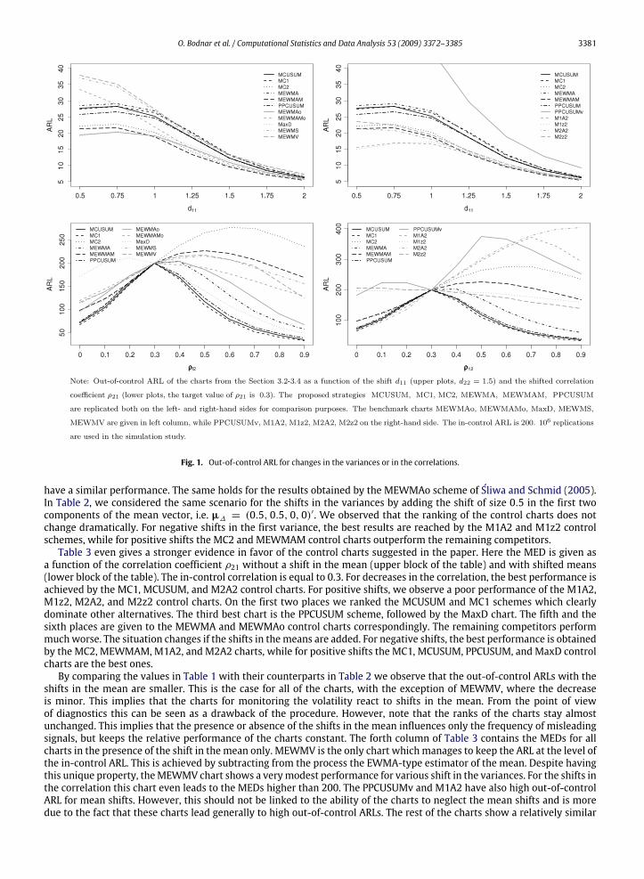
standardized control charts discussed in Remark 2 (see Section 3.3), because their performance is very similar to theperformance of the non-standardized counterparts. Moreover, we skipped the results for Hotelling’s T 2 chart, since itprovided the worst results and made the figures less readable. Fig. 1 shows the behaviour of the out-of-control ARL. Thetwo upper figures show ARL as a function of the shift d11. The shift d22 is set to 1.5 and there is no shift in the mean vector.In the lower figures the correlation coefficient ρ12 is shifted. The in-control value is 0.3. For this value the out-of-controlARL coincides with the in-control ARL of 200. The grey lines on the left-hand figures correspond to MEWMAo, MEWMAMo,MaxD, MEWMS, MEWMV. The grey lines on the right-hand side show the ARL for PPCUSUMv, M1A2, M1z2, M2A2, M2z2schemes. The black lines correspond to the control charts based on the transformed quantities and are replicated on the leftand on the right-hand sides for comparison purposes. MEWMAo, MaxD, M1A2 and M2z2 outperform the proposed chartsfor decreases in the variance. However, MEWMAM and MC2 show uniformly better performance for increases in variances.A similar situation is observed for shifts in the correlations, however, here the advantages of the MCUSUM and MC2 chartsare much more evident. For example, for the out-of-control correlation of 0.6 the best proposed chart leads to the ARL of78.85, while the best benchmark provides the ARL of 107.92.Note that all out-of-control ARLs for shifts in variances are lower than the in-control ARL of 200. This is consistent with

the idea of the ARL as a performance measure. However, for the shift in correlations several charts lead to an out-of-controlARL which is higher than 200. Such behaviour of control charts is particularly dangerous. This occurs in our study for twoproposed charts (MC2 and MEWMAM) and several benchmarks (M1A2, M1z2, MEWMS, MEWMV, PPCUSUMv). The controlstatistics reduce the dimensionality of the process and cause information loss, which leads to reduction in the sensitivityof the control statistics to shifts. In our case this is particularly important for the correlation coefficients which have a verycomplex functional impact on the behaviour of the control statistics. This shows the need for new types of control statisticswhich correctly react to arbitrary shifts in the model parameters.Tables 1–3 summarize the results onMED. Table 1 refers to the case with shifts in the variances. In Table 2 we considered

an additional shift in themean vector. Both tables provide a similar evidence as the results based on theARL. First,we observea good performance of the MEWMA control charts suggested by Reynolds and Cho (2006). If the first variance decreases,then theM1A2 andM1z2 control schemes are the two best charts. On the third place we rank theMaxD scheme followed bythe MEWMAM, MC2 and MEWMAo control charts. For positive shifts, the best performance is achieved by the MEWMAMcontrol scheme, while the MC2 chart is the second best scheme. In this case the M1A2, M1z2, M2A2, and M2z2 approaches


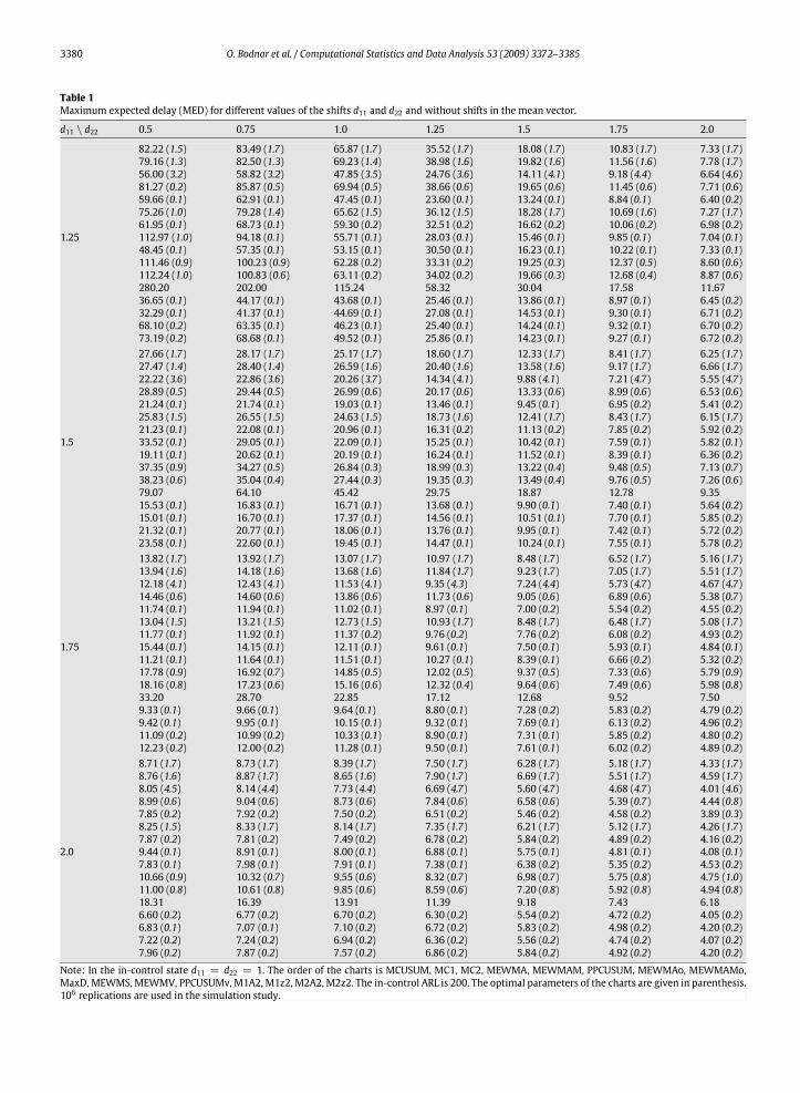
Table 1Maximum expected delay (MED) for different values of the shifts d11 and d22 and without shifts in the mean vector.

d11 \ d22 0.5 0.75 1.0 1.25 1.5 1.75 2.0

82.22 (1.5) 83.49 (1.7) 65.87 (1.7) 35.52 (1.7) 18.08 (1.7) 10.83 (1.7) 7.33 (1.7)79.16 (1.3) 82.50 (1.3) 69.23 (1.4) 38.98 (1.6) 19.82 (1.6) 11.56 (1.6) 7.78 (1.7)56.00 (3.2) 58.82 (3.2) 47.85 (3.5) 24.76 (3.6) 14.11 (4.1) 9.18 (4.4) 6.64 (4.6)81.27 (0.2) 85.87 (0.5) 69.94 (0.5) 38.66 (0.6) 19.65 (0.6) 11.45 (0.6) 7.71 (0.6)59.66 (0.1) 62.91 (0.1) 47.45 (0.1) 23.60 (0.1) 13.24 (0.1) 8.84 (0.1) 6.40 (0.2)75.26 (1.0) 79.28 (1.4) 65.62 (1.5) 36.12 (1.5) 18.28 (1.7) 10.69 (1.6) 7.27 (1.7)61.95 (0.1) 68.73 (0.1) 59.30 (0.2) 32.51 (0.2) 16.62 (0.2) 10.06 (0.2) 6.98 (0.2)

1.25 112.97 (1.0) 94.18 (0.1) 55.71 (0.1) 28.03 (0.1) 15.46 (0.1) 9.85 (0.1) 7.04 (0.1)48.45 (0.1) 57.35 (0.1) 53.15 (0.1) 30.50 (0.1) 16.23 (0.1) 10.22 (0.1) 7.33 (0.1)111.46 (0.9) 100.23 (0.9) 62.28 (0.2) 33.31 (0.2) 19.25 (0.3) 12.37 (0.5) 8.60 (0.6)112.24 (1.0) 100.83 (0.6) 63.11 (0.2) 34.02 (0.2) 19.66 (0.3) 12.68 (0.4) 8.87 (0.6)280.20 202.00 115.24 58.32 30.04 17.58 11.6736.65 (0.1) 44.17 (0.1) 43.68 (0.1) 25.46 (0.1) 13.86 (0.1) 8.97 (0.1) 6.45 (0.2)32.29 (0.1) 41.37 (0.1) 44.69 (0.1) 27.08 (0.1) 14.53 (0.1) 9.30 (0.1) 6.71 (0.2)68.10 (0.2) 63.35 (0.1) 46.23 (0.1) 25.40 (0.1) 14.24 (0.1) 9.32 (0.1) 6.70 (0.2)73.19 (0.2) 68.68 (0.1) 49.52 (0.1) 25.86 (0.1) 14.23 (0.1) 9.27 (0.1) 6.72 (0.2)27.66 (1.7) 28.17 (1.7) 25.17 (1.7) 18.60 (1.7) 12.33 (1.7) 8.41 (1.7) 6.25 (1.7)27.47 (1.4) 28.40 (1.4) 26.59 (1.6) 20.40 (1.6) 13.58 (1.6) 9.17 (1.7) 6.66 (1.7)22.22 (3.6) 22.86 (3.6) 20.26 (3.7) 14.34 (4.1) 9.88 (4.1) 7.21 (4.7) 5.55 (4.7)28.89 (0.5) 29.44 (0.5) 26.99 (0.6) 20.17 (0.6) 13.33 (0.6) 8.99 (0.6) 6.53 (0.6)21.24 (0.1) 21.74 (0.1) 19.03 (0.1) 13.46 (0.1) 9.45 (0.1) 6.95 (0.2) 5.41 (0.2)25.83 (1.5) 26.55 (1.5) 24.63 (1.5) 18.73 (1.6) 12.41 (1.7) 8.43 (1.7) 6.15 (1.7)21.23 (0.1) 22.08 (0.1) 20.96 (0.1) 16.31 (0.2) 11.13 (0.2) 7.85 (0.2) 5.92 (0.2)

1.5 33.52 (0.1) 29.05 (0.1) 22.09 (0.1) 15.25 (0.1) 10.42 (0.1) 7.59 (0.1) 5.82 (0.1)19.11 (0.1) 20.62 (0.1) 20.19 (0.1) 16.24 (0.1) 11.52 (0.1) 8.39 (0.1) 6.36 (0.2)37.35 (0.9) 34.27 (0.5) 26.84 (0.3) 18.99 (0.3) 13.22 (0.4) 9.48 (0.5) 7.13 (0.7)38.23 (0.6) 35.04 (0.4) 27.44 (0.3) 19.35 (0.3) 13.49 (0.4) 9.76 (0.5) 7.26 (0.6)79.07 64.10 45.42 29.75 18.87 12.78 9.3515.53 (0.1) 16.83 (0.1) 16.71 (0.1) 13.68 (0.1) 9.90 (0.1) 7.40 (0.1) 5.64 (0.2)15.01 (0.1) 16.70 (0.1) 17.37 (0.1) 14.56 (0.1) 10.51 (0.1) 7.70 (0.1) 5.85 (0.2)21.32 (0.1) 20.77 (0.1) 18.06 (0.1) 13.76 (0.1) 9.95 (0.1) 7.42 (0.1) 5.72 (0.2)23.58 (0.1) 22.60 (0.1) 19.45 (0.1) 14.47 (0.1) 10.24 (0.1) 7.55 (0.1) 5.78 (0.2)13.82 (1.7) 13.92 (1.7) 13.07 (1.7) 10.97 (1.7) 8.48 (1.7) 6.52 (1.7) 5.16 (1.7)13.94 (1.6) 14.18 (1.6) 13.68 (1.6) 11.84 (1.7) 9.23 (1.7) 7.05 (1.7) 5.51 (1.7)12.18 (4.1) 12.43 (4.1) 11.53 (4.1) 9.35 (4.3) 7.24 (4.4) 5.73 (4.7) 4.67 (4.7)14.46 (0.6) 14.60 (0.6) 13.86 (0.6) 11.73 (0.6) 9.05 (0.6) 6.89 (0.6) 5.38 (0.7)11.74 (0.1) 11.94 (0.1) 11.02 (0.1) 8.97 (0.1) 7.00 (0.2) 5.54 (0.2) 4.55 (0.2)13.04 (1.5) 13.21 (1.5) 12.73 (1.5) 10.93 (1.7) 8.48 (1.7) 6.48 (1.7) 5.08 (1.7)11.77 (0.1) 11.92 (0.1) 11.37 (0.2) 9.76 (0.2) 7.76 (0.2) 6.08 (0.2) 4.93 (0.2)

1.75 15.44 (0.1) 14.15 (0.1) 12.11 (0.1) 9.61 (0.1) 7.50 (0.1) 5.93 (0.1) 4.84 (0.1)11.21 (0.1) 11.64 (0.1) 11.51 (0.1) 10.27 (0.1) 8.39 (0.1) 6.66 (0.2) 5.32 (0.2)17.78 (0.9) 16.92 (0.7) 14.85 (0.5) 12.02 (0.5) 9.37 (0.5) 7.33 (0.6) 5.79 (0.9)18.16 (0.8) 17.23 (0.6) 15.16 (0.6) 12.32 (0.4) 9.64 (0.6) 7.49 (0.6) 5.98 (0.8)33.20 28.70 22.85 17.12 12.68 9.52 7.509.33 (0.1) 9.66 (0.1) 9.64 (0.1) 8.80 (0.1) 7.28 (0.2) 5.83 (0.2) 4.79 (0.2)9.42 (0.1) 9.95 (0.1) 10.15 (0.1) 9.32 (0.1) 7.69 (0.1) 6.13 (0.2) 4.96 (0.2)11.09 (0.2) 10.99 (0.2) 10.33 (0.1) 8.90 (0.1) 7.31 (0.1) 5.85 (0.2) 4.80 (0.2)12.23 (0.2) 12.00 (0.2) 11.28 (0.1) 9.50 (0.1) 7.61 (0.1) 6.02 (0.2) 4.89 (0.2)8.71 (1.7) 8.73 (1.7) 8.39 (1.7) 7.50 (1.7) 6.28 (1.7) 5.18 (1.7) 4.33 (1.7)8.76 (1.6) 8.87 (1.7) 8.65 (1.6) 7.90 (1.7) 6.69 (1.7) 5.51 (1.7) 4.59 (1.7)8.05 (4.5) 8.14 (4.4) 7.73 (4.4) 6.69 (4.7) 5.60 (4.7) 4.68 (4.7) 4.01 (4.6)8.99 (0.6) 9.04 (0.6) 8.73 (0.6) 7.84 (0.6) 6.58 (0.6) 5.39 (0.7) 4.44 (0.8)7.85 (0.2) 7.92 (0.2) 7.50 (0.2) 6.51 (0.2) 5.46 (0.2) 4.58 (0.2) 3.89 (0.3)8.25 (1.5) 8.33 (1.7) 8.14 (1.7) 7.35 (1.7) 6.21 (1.7) 5.12 (1.7) 4.26 (1.7)7.87 (0.2) 7.81 (0.2) 7.49 (0.2) 6.78 (0.2) 5.84 (0.2) 4.89 (0.2) 4.16 (0.2)

2.0 9.44 (0.1) 8.91 (0.1) 8.00 (0.1) 6.88 (0.1) 5.75 (0.1) 4.81 (0.1) 4.08 (0.1)7.83 (0.1) 7.98 (0.1) 7.91 (0.1) 7.38 (0.1) 6.38 (0.2) 5.35 (0.2) 4.53 (0.2)10.66 (0.9) 10.32 (0.7) 9.55 (0.6) 8.32 (0.7) 6.98 (0.7) 5.75 (0.8) 4.75 (1.0)11.00 (0.8) 10.61 (0.8) 9.85 (0.6) 8.59 (0.6) 7.20 (0.8) 5.92 (0.8) 4.94 (0.8)18.31 16.39 13.91 11.39 9.18 7.43 6.186.60 (0.2) 6.77 (0.2) 6.70 (0.2) 6.30 (0.2) 5.54 (0.2) 4.72 (0.2) 4.05 (0.2)6.83 (0.1) 7.07 (0.1) 7.10 (0.2) 6.72 (0.2) 5.83 (0.2) 4.98 (0.2) 4.20 (0.2)7.22 (0.2) 7.24 (0.2) 6.94 (0.2) 6.36 (0.2) 5.56 (0.2) 4.74 (0.2) 4.07 (0.2)7.96 (0.2) 7.87 (0.2) 7.57 (0.2) 6.86 (0.2) 5.84 (0.2) 4.92 (0.2) 4.20 (0.2)

Note: In the in-control state d11 = d22 = 1. The order of the charts is MCUSUM, MC1, MC2, MEWMA, MEWMAM, PPCUSUM, MEWMAo, MEWMAMo,MaxD, MEWMS, MEWMV, PPCUSUMv, M1A2, M1z2, M2A2, M2z2. The in-control ARL is 200. The optimal parameters of the charts are given in parenthesis.106 replications are used in the simulation study.


Fig. 1. Out-of-control ARL for changes in the variances or in the correlations.

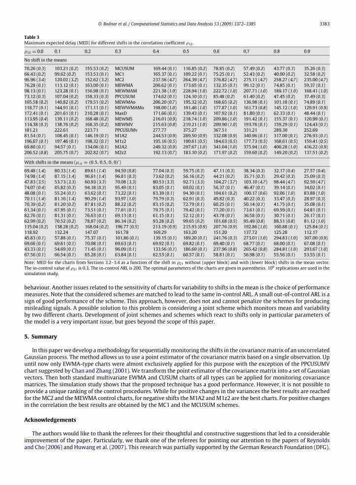
have a similar performance. The same holds for the results obtained by the MEWMAo scheme of Śliwa and Schmid (2005).In Table 2, we considered the same scenario for the shifts in the variances by adding the shift of size 0.5 in the first twocomponents of the mean vector, i.e. µ∆ = (0.5, 0.5, 0, 0)′. We observed that the ranking of the control charts does notchange dramatically. For negative shifts in the first variance, the best results are reached by the M1A2 and M1z2 controlschemes, while for positive shifts the MC2 and MEWMAM control charts outperform the remaining competitors.Table 3 even gives a stronger evidence in favor of the control charts suggested in the paper. Here the MED is given as

a function of the correlation coefficient ρ21 without a shift in the mean (upper block of the table) and with shifted means(lower block of the table). The in-control correlation is equal to 0.3. For decreases in the correlation, the best performance isachieved by the MC1, MCUSUM, and M2A2 control charts. For positive shifts, we observe a poor performance of the M1A2,M1z2, M2A2, and M2z2 control charts. On the first two places we ranked the MCUSUM and MC1 schemes which clearlydominate other alternatives. The third best chart is the PPCUSUM scheme, followed by the MaxD chart. The fifth and thesixth places are given to the MEWMA and MEWMAo control charts correspondingly. The remaining competitors performmuchworse. The situation changes if the shifts in themeans are added. For negative shifts, the best performance is obtainedby the MC2, MEWMAM, M1A2, and M2A2 charts, while for positive shifts the MC1, MCUSUM, PPCUSUM, and MaxD controlcharts are the best ones.By comparing the values in Table 1 with their counterparts in Table 2 we observe that the out-of-control ARLs with the

shifts in the mean are smaller. This is the case for all of the charts, with the exception of MEWMV, where the decreaseis minor. This implies that the charts for monitoring the volatility react to shifts in the mean. From the point of viewof diagnostics this can be seen as a drawback of the procedure. However, note that the ranks of the charts stay almostunchanged. This implies that the presence or absence of the shifts in the mean influences only the frequency of misleadingsignals, but keeps the relative performance of the charts constant. The forth column of Table 3 contains the MEDs for allcharts in the presence of the shift in the mean only. MEWMV is the only chart which manages to keep the ARL at the level ofthe in-control ARL. This is achieved by subtracting from the process the EWMA-type estimator of the mean. Despite havingthis unique property, theMEWMV chart shows a verymodest performance for various shift in the variances. For the shifts inthe correlation this chart even leads to the MEDs higher than 200. The PPCUSUMv and M1A2 have also high out-of-controlARL for mean shifts. However, this should not be linked to the ability of the charts to neglect the mean shifts and is moredue to the fact that these charts lead generally to high out-of-control ARLs. The rest of the charts show a relatively similar


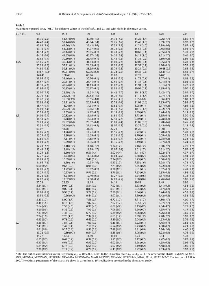
Table 2Maximum expected delay (MED) for different values of the shifts d11 and d22 and with shifts in the mean vector.

d11 \ d22 0.5 0.75 1.0 1.25 1.5 1.75 2.0

45.35 (0.5) 51.47 (0.9) 40.50 (1.5) 24.31 (1.5) 14.25 (1.7) 9.26 (1.7) 6.66 (1.7)44.42 (0.4) 52.44 (0.8) 43.84 (1.4) 26.75 (1.6) 15.49 (1.6) 9.89 (1.7) 6.97 (1.7)43.63 (3.4) 42.66 (3.5) 29.42 (3.6) 17.53 (3.9) 11.24 (4.0) 7.89 (4.6) 5.97 (4.6)43.16 (0.1) 51.08 (0.1) 44.07 (0.5) 26.72 (0.5) 15.52 (0.6) 9.85 (0.6) 6.94 (0.7)44.14 (0.1) 42.14 (0.1) 28.05 (0.1) 16.41 (0.1) 10.68 (0.1) 7.65 (0.2) 5.78 (0.2)44.14 (0.6) 49.33 (0.9) 40.17 (1.4) 24.36 (1.4) 14.19 (1.6) 9.11 (1.7) 6.46 (1.7)30.68 (0.1) 30.10 (0.1) 25.45 (0.1) 17.48 (0.2) 11.35 (0.2) 7.89 (0.2) 5.95 (0.2)

1.25 65.65 (0.1) 49.66 (0.1) 31.83 (0.1) 19.00 (0.1) 12.02 (0.1) 8.35 (0.1) 6.28 (0.1)35.25 (0.1) 35.71 (0.1) 29.33 (0.1) 19.26 (0.1) 12.37 (0.1) 8.70 (0.1) 6.52 (0.2)74.60 (0.8) 59.81 (0.2) 38.35 (0.2) 23.79 (0.3) 15.24 (0.4) 10.48 (0.5) 7.65 (0.6)110.71 (1.0) 99.71 (0.9) 62.96 (0.2) 33.74 (0.2) 19.38 (0.4) 12.38 (0.5) 8.58 (0.7)148.45 108.48 68.06 39.02 22.78 14.60 10.2229.96 (0.1) 33.46 (0.1) 30.36 (0.1) 18.99 (0.1) 11.73 (0.1) 8.07 (0.1) 6.02 (0.2)26.57 (0.1) 29.31 (0.1) 26.41 (0.1) 17.50 (0.1) 11.37 (0.1) 8.01 (0.1) 6.03 (0.2)46.10 (0.1) 42.24 (0.1) 31.13 (0.1) 19.02 (0.1) 11.91 (0.1) 8.31 (0.1) 6.22 (0.2)41.94 (0.1) 36.95 (0.1) 26.77 (0.1) 16.81 (0.1) 10.94 (0.1) 7.88 (0.1) 6.00 (0.2)22.00 (1.5) 21.99 (1.5) 19.31 (1.5) 14.41 (1.7) 10.18 (1.7) 7.42 (1.7) 5.69 (1.7)22.39 (1.4) 22.62 (1.4) 20.53 (1.6) 15.79 (1.6) 11.13 (1.7) 7.97 (1.7) 6.02 (1.7)19.47 (3.9) 19.03 (3.9) 15.55 (4.0) 11.46 (4.2) 8.35 (4.4) 6.36 (4.7) 5.08 (4.7)22.88 (0.4) 23.11 (0.5) 20.75 (0.5) 15.78 (0.6) 11.01 (0.6) 7.85 (0.7) 5.93 (0.7)18.47 (0.1) 18.04 (0.1) 14.61 (0.1) 10.82 (0.1) 8.08 (0.1) 6.17 (0.2) 4.95 (0.2)20.89 (1.4) 20.92 (1.4) 18.86 (1.4) 14.38 (1.5) 10.16 (1.7) 7.32 (1.7) 5.55 (1.7)15.75 (0.1) 15.55 (0.1) 14.12 (0.2) 11.18 (0.2) 8.39 (0.2) 6.44 (0.2) 5.11 (0.2)

1.5 24.08 (0.1) 20.82 (0.1) 16.15 (0.1) 11.89 (0.1) 8.73 (0.1) 6.65 (0.1) 5.30 (0.1)16.41 (0.1) 16.58 (0.1) 15.33 (0.1) 12.40 (0.1) 9.39 (0.1) 7.28 (0.2) 5.69 (0.2)28.83 (0.5) 25.57 (0.4) 20.37 (0.4) 15.09 (0.4) 11.05 (0.5) 8.28 (0.6) 6.45 (0.8)37.52 (0.9) 34.44 (0.5) 27.11 (0.3) 19.07 (0.3) 13.23 (0.4) 9.43 (0.6) 7.11 (0.8)53.07 43.28 31.95 22.22 15.29 11.01 8.4014.05 (0.1) 14.76 (0.1) 14.21 (0.1) 11.55 (0.1) 8.72 (0.1) 6.70 (0.2) 5.28 (0.2)13.55 (0.1) 14.20 (0.1) 13.69 (0.1) 11.31 (0.1) 8.70 (0.1) 6.69 (0.2) 5.29 (0.2)17.80 (0.1) 17.11 (0.1) 14.85 (0.1) 11.59 (0.1) 8.72 (0.1) 6.78 (0.2) 5.33 (0.2)18.03 (0.1) 16.89 (0.1) 14.35 (0.1) 11.16 (0.1) 8.49 (0.1) 6.57 (0.2) 5.24 (0.2)12.28 (1.7) 12.18 (1.7) 11.18 (1.7) 9.34 (1.7) 7.46 (1.7) 5.90 (1.7) 4.79 (1.7)12.43 (1.5) 12.48 (1.5) 11.79 (1.7) 10.07 (1.6) 8.01 (1.7) 6.31 (1.7) 5.07 (1.7)11.25 (4.3) 11.10 (4.5) 9.81 (4.4) 8.02 (4.4) 6.41 (4.7) 5.22 (4.7) 4.37 (4.7)12.77 (0.5) 12.73 (0.5) 11.93 (0.6) 10.04 (0.6) 7.88 (0.7) 6.16 (0.7) 4.94 (0.8)10.88 (0.1) 10.69 (0.1) 9.49 (0.1) 7.74 (0.2) 6.23 (0.2) 5.06 (0.2) 4.25 (0.2)11.66 (1.4) 11.69 (1.6) 10.93 (1.6) 9.23 (1.7) 7.35 (1.6) 5.78 (1.7) 4.71 (1.7)9.90 (0.2) 9.68 (0.2) 8.96 (0.2) 7.71 (0.2) 6.35 (0.2) 5.22 (0.2) 4.37 (0.2)

1.75 12.80 (0.1) 11.72 (0.1) 10.02 (0.1) 8.20 (0.1) 6.61 (0.1) 5.37 (0.1) 4.48 (0.1)10.25 (0.1) 10.33 (0.1) 9.91 (0.1) 8.76 (0.1) 7.23 (0.2) 5.93 (0.2) 4.91 (0.2)15.24 (0.8) 14.24 (0.5) 12.40 (0.5) 10.27 (0.5) 8.24 (0.6) 6.57 (0.6) 5.32 (1.0)17.87 (0.9) 17.02 (0.7) 14.88 (0.5) 12.00 (0.5) 9.38 (0.6) 7.26 (0.6) 5.80 (0.8)25.58 22.35 18.15 14.11 10.88 8.49 6.868.84 (0.1) 9.04 (0.1) 8.84 (0.1) 7.92 (0.1) 6.63 (0.2) 5.41 (0.2) 4.51 (0.2)8.83 (0.1) 9.05 (0.1) 8.89 (0.1) 8.01 (0.1) 6.65 (0.2) 5.47 (0.2) 4.55 (0.2)10.09 (0.2) 9.99 (0.1) 9.22 (0.1) 7.99 (0.1) 6.64 (0.1) 5.44 (0.2) 4.53 (0.2)10.54 (0.2) 10.26 (0.2) 9.44 (0.1) 8.07 (0.1) 6.60 (0.2) 5.42 (0.2) 4.51 (0.2)8.13 (1.7) 8.00 (1.7) 7.56 (1.7) 6.72 (1.7) 5.71 (1.7) 4.80 (1.7) 4.09 (1.7)8.18 (1.6) 8.18 (1.7) 7.87 (1.7) 7.07 (1.7) 6.05 (1.7) 5.07 (1.7) 4.29 (1.7)7.64 (4.7) 7.55 (4.5) 6.96 (4.6) 6.02 (4.7) 5.13 (4.7) 4.34 (4.7) 3.79 (4.7)8.40 (0.6) 8.32 (0.6) 7.93 (0.6) 7.06 (0.7) 5.96 (0.7) 4.95 (0.7) 4.15 (0.8)7.43 (0.2) 7.35 (0.2) 6.77 (0.2) 5.89 (0.2) 4.98 (0.2) 4.26 (0.3) 3.65 (0.3)7.74 (1.6) 7.70 (1.7) 7.34 (1.7) 6.61 (1.7) 5.59 (1.7) 4.70 (1.7) 3.99 (1.7)6.93 (0.2) 6.78 (0.2) 6.43 (0.2) 5.80 (0.2) 5.04 (0.2) 4.33 (0.2) 3.76 (0.2)

2.0 8.36 (0.1) 7.87 (0.1) 7.09 (0.1) 6.15 (0.1) 5.22 (0.1) 4.45 (0.1) 3.84 (0.1)7.41 (0.1) 7.42 (0.1) 7.18 (0.2) 6.54 (0.2) 5.73 (0.2) 4.90 (0.2) 4.21 (0.2)9.61 (0.9) 9.25 (0.9) 8.56 (0.6) 7.48 (0.6) 6.31 (0.9) 5.26 (1.0) 4.40 (1.0)10.72 (0.9) 10.39 (0.7) 9.54 (0.7) 8.35 (0.6) 6.96 (0.8) 5.73 (0.9) 4.76 (0.9)15.27 13.84 11.89 10.00 8.23 6.83 5.786.35 (0.2) 6.42 (0.2) 6.32 (0.2) 5.85 (0.2) 5.17 (0.2) 4.47 (0.2) 3.87 (0.2)6.53 (0.2) 6.61 (0.2) 6.53 (0.2) 6.02 (0.2) 5.28 (0.2) 4.55 (0.2) 3.96 (0.2)6.84 (0.2) 6.78 (0.2) 6.51 (0.2) 5.92 (0.2) 5.19 (0.2) 4.48 (0.2) 3.89 (0.2)7.29 (0.2) 7.17 (0.2) 6.79 (0.2) 6.11 (0.2) 5.27 (0.2) 4.53 (0.2) 3.92 (0.2)

Note: The out-of-control mean vector is given by µ∆ = (0.5, 0.5, 0, 0)′ . In the in-control state d11 = d22 = 1. The order of the charts is MCUSUM, MC1,MC2, MEWMA, MEWMAM, PPCUSUM, MEWMAo, MEWMAMo, MaxD, MEWMS, MEWMV, PPCUSUMv, M1A2, M1z2, M2A2, M2z2. The in-control ARL is200. The optimal parameters of the charts are given in parenthesis. 106 replications are used in the simulation study.


Table 3Maximum expected delay (MED) for different shifts in the correlation coefficient ρ12 .

ρ12 = 0.0 0.1 0.2 0.3 0.4 0.5 0.6 0.7 0.8 0.9

No shift in the means

70.26 (0.3) 103.21 (0.2) 155.53 (0.2) MCUSUM 169.44 (0.1) 116.85 (0.2) 78.85 (0.2) 57.49 (0.2) 43.77 (0.3) 35.26 (0.3)66.43 (0.2) 99.62 (0.2) 153.53 (0.1) MC1 165.37 (0.1) 109.22 (0.1) 75.25 (0.1) 52.43 (0.2) 40.00 (0.2) 32.58 (0.2)96.96 (3.4) 120.02 (3.2) 152.62 (3.2) MC2 237.56 (4.7) 264.39 (4.7) 276.82 (4.7) 275.11 (4.7) 258.27 (4.7) 235.00 (4.7)76.28 (0.1) 113.12 (0.1) 163.00 (0.1) MEWMA 206.62 (0.1) 173.65 (0.1) 132.35 (0.1) 99.12 (0.1) 74.85 (0.1) 59.37 (0.1)98.13 (0.1) 123.28 (0.1) 156.98 (0.1) MEWMAM 221.38 (1.0) 228.94 (1.0) 222.72 (1.0) 207.71 (1.0) 189.17 (1.0) 168.41 (1.0)73.12 (0.3) 107.04 (0.2) 158.33 (0.3) PPCUSUM 174.62 (0.1) 124.10 (0.1) 85.48 (0.2) 61.40 (0.2) 47.45 (0.2) 37.49 (0.3)105.58 (0.2) 140.82 (0.2) 179.51 (0.2) MEWMAo 206.20 (0.7) 195.32 (0.2) 168.65 (0.2) 136.98 (0.1) 101.18 (0.1) 74.89 (0.1)118.77 (0.1) 144.91 (0.1) 171.11 (0.1) MEWWMAMo 198.00 (1.0) 191.46 (1.0) 177.87 (1.0) 161.73 (0.8) 145.12 (1.0) 129.91 (0.9)172.41 (0.1) 201.61 (0.1) 210.28 (0.1) MaxD 171.66 (0.1) 139.43 (0.1) 107.92 (0.1) 81.80 (0.1) 62.33 (0.1) 48.44 (0.1)113.95 (0.4) 139.11 (0.2) 168.48 (0.2) MEWMS 216.01 (0.9) 218.74 (1.0) 209.86 (1.0) 191.42 (0.1) 155.37 (0.1) 120.99 (0.1)114.38 (0.3) 138.76 (0.2) 168.35 (0.2) MEWMV 215.63 (0.8) 219.21 (1.0) 209.90 (1.0) 193.76 (0.1) 159.29 (0.1) 124.43 (0.1)181.21 222.61 223.71 PPCUSUMv 277.77 375.27 367.51 331.21 289.30 252.6981.54 (0.1) 108.45 (0.1) 146.19 (0.1) M1A2 244.53 (0.9) 289.50 (0.9) 332.08 (0.9) 340.96 (0.1) 317.00 (0.1) 276.93 (0.1)196.67 (0.1) 197.46 (0.1) 198.32 (0.1) M1z2 195.16 (0.5) 190.61 (0.5) 184.63 (0.5) 177.73 (0.5) 168.61 (0.5) 159.41 (0.5)69.80 (0.1) 94.57 (0.1) 134.06 (0.1) M2A2 249.32 (0.9) 297.67 (1.0) 341.04 (1.0) 375.94 (1.0) 400.28 (1.0) 416.22 (0.9)206.52 (0.8) 205.75 (0.7) 202.82 (0.7) M2z2 192.13 (0.7) 183.10 (0.2) 171.97 (0.2) 159.60 (0.2) 149.20 (0.2) 137.51 (0.2)

With shifts in the means (µ∆ = (0.5, 0.5, 0, 0)′)

69.48 (1.4) 80.33 (1.4) 89.61 (1.4) 94.50 (0.8) 77.04 (0.3) 59.75 (0.3) 47.11 (0.3) 38.34 (0.3) 32.17 (0.4) 27.57 (0.4)74.98 (1.4) 87.15 (1.4) 96.61 (1.4) 96.81 (0.3) 73.62 (0.2) 56.16 (0.2) 44.21 (0.2) 35.71 (0.3) 29.42 (0.3) 25.09 (0.3)47.83 (3.5) 53.73 (3.3) 60.93 (3.3) 70.08 (3.3) 80.53 (3.3) 92.71 (3.3) 104.27 (3.7) 103.10 (4.7) 98.44 (4.7) 92.50 (4.7)74.07 (0.4) 85.82 (0.3) 94.18 (0.3) 95.49 (0.1) 83.05 (0.1) 69.02 (0.1) 56.37 (0.1) 46.47 (0.1) 39.14 (0.1) 34.02 (0.1)48.08 (0.1) 55.24 (0.1) 63.62 (0.1) 73.22 (0.1) 83.39 (0.1) 94.30 (0.1) 104.61 (0.2) 100.17 (0.6) 92.06 (1.0) 83.88 (1.0)70.11 (1.4) 81.16 (1.4) 90.29 (1.4) 93.97 (1.0) 79.79 (0.3) 62.91 (0.3) 49.82 (0.3) 40.22 (0.3) 33.47 (0.3) 28.97 (0.3)70.39 (0.2) 81.20 (0.2) 87.81 (0.2) 88.22 (0.2) 83.15 (0.2) 72.79 (0.1) 60.25 (0.1) 50.14 (0.1) 41.75 (0.1) 35.08 (0.1)61.34 (0.1) 67.95 (0.1) 73.51 (0.1) 77.61 (0.1) 79.75 (0.1) 79.42 (0.1) 77.20 (0.1) 73.61 (0.1) 69.59 (0.1) 64.81 (0.1)82.76 (0.1) 81.31 (0.1) 76.63 (0.1) 69.13 (0.1) 61.15 (0.1) 52.12 (0.1) 43.78 (0.1) 36.58 (0.1) 30.71 (0.1) 26.17 (0.1)62.99 (0.2) 70.52 (0.2) 78.87 (0.2) 86.34 (0.2) 93.28 (0.2) 99.65 (0.2) 101.68 (0.5) 95.49 (0.8) 88.51 (0.8) 81.12 (1.0)115.04 (0.2) 138.28 (0.2) 168.04 (0.2) 196.77 (0.5) 213.19 (0.9) 215.93 (0.9) 207.76 (0.9) 192.86 (1.0) 160.88 (0.1) 125.84 (0.1)118.92 132.24 147.07 161.78 169.29 163.20 151.20 137.72 125.28 112.1745.83 (0.1) 57.88 (0.1) 75.37 (0.1) 101.86 (0.1) 139.15 (0.1) 189.20 (0.1) 241.76 (0.3) 273.01 (1.0) 294.83 (1.0) 307.00 (0.9)69.66 (0.1) 69.61 (0.1) 70.08 (0.1) 69.63 (0.1) 69.92 (0.1) 69.82 (0.1) 69.40 (0.1) 68.77 (0.1) 68.00 (0.1) 67.08 (0.1)43.33 (0.1) 54.69 (0.1) 71.45 (0.1) 96.09 (0.1) 133.56 (0.1) 186.60 (0.1) 237.96 (0.8) 265.42 (0.8) 284.81 (1.0) 293.67 (1.0)67.56 (0.1) 66.54 (0.1) 65.28 (0.1) 63.84 (0.1) 62.53 (0.1) 60.57 (0.1) 58.81 (0.1) 56.98 (0.1) 55.56 (0.1) 53.55 (0.1)

Note: MED for the charts from Sections 3.2–3.4 as a function of the shift in ρ21 without (upper block) and with (lower block) shifts in the mean vector.The in-control value of ρ21 is 0.3. The in-control ARL is 200. The optimal parameters of the charts are given in parenthesis. 106 replications are used in thesimulation study.

behaviour. Another issues related to the sensitivity of charts for variability to shifts in themean is the choice of performancemeasures. Note that the considered schemes are matched to lead to the same in-control ARL. A small out-of-control ARL is asign of good performance of the scheme. This approach, however, does not and cannot penalize the schemes for producingmisleading signals. A possible solution to this problem is considering a joint scheme which monitors mean and variabilityby two different charts. Development of joint schemes and schemes which react to shifts only in particular parameters ofthe model is a very important issue, but goes beyond the scope of this paper.

5. Summary

In this paperwe develop amethodology for sequentiallymonitoring the shifts in the covariancematrix of an uncorrelatedGaussian process. The method allows us to use a point estimator of the covariance matrix based on a single observation. Upuntil now only EWMA-type charts were almost exclusively applied for this purpose with the exception of the PPCUSUMVchart suggested by Chan and Zhang (2001). We transform the point estimator of the covariancematrix into a set of Gaussianvectors. Then both standard multivariate EWMA and CUSUM charts of all types can be applied for monitoring covariancematrices. The simulation study shows that the proposed technique has a good performance. However, it is not possible toprovide a unique ranking of the control procedures. While for positive changes in the variances the best results are reachedfor theMC2 and theMEWMA control charts, for negative shifts theM1A2 andM1z2 are the best charts. For positive changesin the correlation the best results are obtained by the MC1 and the MCUSUM schemes.

Acknowledgements

The authors would like to thank the referees for their thoughtful and constructive suggestions that led to a considerableimprovement of the paper. Particularly, we thank one of the referees for pointing our attention to the papers of Reynoldsand Cho (2006) and Huwang et al. (2007). This research was partially supported by the German Research Foundation (DFG).


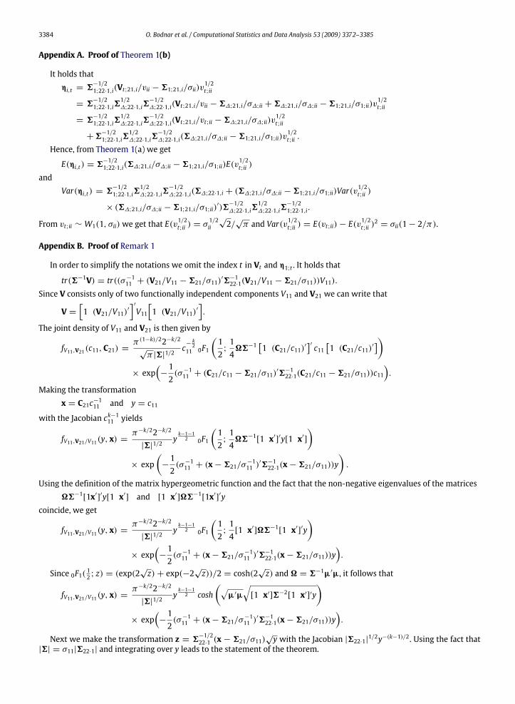
Appendix A. Proof of Theorem 1(b)

It holds thatηi,t = 6

−1/21;22·1,i(Vt;21,i/vii − 61;21,i/σii)v

1/2t;ii

= 6−1/21;22·1,i6

1/2∆;22·1,i6

−1/2∆;22·1,i(Vt;21,i/vii − 6∆;21,i/σ∆;ii + 6∆;21,i/σ∆;ii − 61;21,i/σ1;ii)v

1/2t;ii

= 6−1/21;22·1,i6

1/2∆;22·1,i6

−1/2∆;22·1,i(Vt;21,i/vt;ii − 6∆;21,i/σ∆;ii)v

1/2t;ii

+6−1/21;22·1,i6

1/2∆;22·1,i6

−1/2∆;22·1,i(6∆;21,i/σ∆;ii − 61;21,i/σ1;ii)v

1/2t;ii .

Hence, from Theorem 1(a) we get

E(ηi,t) = 6−1/21;22·1,i(6∆;21,i/σ∆;ii − 61;21,i/σ1;ii)E(v

1/2t;ii )

andVar(ηi,t) = 6

−1/21;22·1,i6

1/2∆;22·1,i6

−1/2∆;22·1,i(6∆;22·1,i + (6∆;21,i/σ∆;ii − 61;21,i/σ1;ii)Var(v

1/2t;ii )

× (6∆;21,i/σ∆;ii − 61;21,i/σ1;ii)′)6−1/2∆;22·1,i6

1/2∆;22·1,i6

−1/21;22·1,i.

From vt;ii ∼ W1(1, σii)we get that E(v1/2t;ii ) = σ

1/2ii

√2/√π and Var(v1/2t;ii ) = E(vt;ii)− E(v

1/2t;ii )

2= σii(1− 2/π).

Appendix B. Proof of Remark 1

In order to simplify the notations we omit the index t in Vt and η1;t . It holds that

tr(6−1V) = tr((σ−111 + (V21/V11 − 621/σ11)′6−122·1(V21/V11 − 621/σ11))V11).

Since V consists only of two functionally independent components V11 and V21 we can write that

V =[1 (V21/V11)′

]′V11[1 (V21/V11)′

].

The joint density of V11 and V21 is then given by

fV11,V21(c11, C21) =π (1−k)/22−k/2√π |6|1/2

c−k2

11 0F1

(12;14�6−1

[1 (C21/c11)′

]′ c11 [1 (C21/c11)′])× exp

(−12(σ−111 + (C21/c11 − 621/σ11)

′6−122·1(C21/c11 − 621/σ11))c11).

Making the transformationx = C21c−111 and y = c11

with the Jacobian ck−111 yields

fV11,V21/V11(y, x) =π−k/22−k/2

|6|1/2yk−1−12 0F1

(12;14�6−1[1 x′]′y[1 x′]

)× exp

(−12(σ−111 + (x− 621/σ

−111 )′6−122·1(x− 621/σ11))y

).

Using the definition of the matrix hypergeometric function and the fact that the non-negative eigenvalues of the matrices�6−1[1x′]′y[1 x′] and [1 x′]�6−1[1x′]′y

coincide, we get

fV11,V21/V11(y, x) =π−k/22−k/2

|6|1/2yk−1−12 0F1

(12;14[1 x′]�6−1[1 x′]′y

)× exp

(−12(σ−111 + (x− 621/σ

−111 )′6−122·1(x− 621/σ11))y

).

Since 0F1( 12 ; z) = (exp(2√z)+ exp(−2

√z))/2 = cosh(2

√z) and� = 6−1µ′µ, it follows that

fV11,V21/V11(y, x) =π−k/22−k/2

|6|1/2yk−1−12 cosh

(√µ′µ

√[1 x′]6−2[1 x′]′y

)× exp

(−12(σ−111 + (x− 621/σ

−111 )′6−122·1(x− 621/σ11))y

).

Next we make the transformation z = 6−1/222·1 (x − 621/σ11)

√y with the Jacobian |622·1|1/2y−(k−1)/2. Using the fact that

|6| = σ11|622·1| and integrating over y leads to the statement of the theorem.


References

Albers, W., Kallenberg, W.C.M., 2004. Are estimated control charts in control? Statistics 38, 67–79.Andersson, E., Bock, D., Frisén, M., 2004. Detection of turning points in business cycles. Journal of Business Cycle Measurement and Analysis 1, 93–108.Bodnar, O., 2007. Sequential procedures for monitoring covariances of asset returns. In: Gregoriou, G.N. (Ed.), Advances in Risk Management. Palgrave,London, pp. 241–264.

Bodnar, T., Okhrin, Y., 2008. Properties of the singular, inverse and generalized inverse partitioned Wishart distributions. Journal of Multivariate Analysis99, 2389–2405.

Chan, L.K., Zhang, J., 2001. Cumulative sum control charts for the covariance matrix. Statistica Sinica 11, 767–790.Conte, S.D., de Boor, C., 1981. Elementary Numerical Analysis. Mc Graw-Hill, London.Crosier, R.B., 1986. A new two-sided cumulative quality control scheme. Technometrics 28, 187–194.Crosier, R.B., 1988. Multivariate generalizations of cumulative sum quality-control schemes. Technometrics 30, 291–303.Frisén, M., 1992. Evaluations of methods for statistical surveillance. Statistics in Medicine 11, 1489–1502.Hawkins, D.M., 1981. A CUSUM for a scale parameter. Journal of Quality Technology 13, 228–231.Hawkins, D.M., 1991. Multivariate quality control based on regression adjusted variables. Technometrics 33, 61–75.Hawkins, D.M., 1993. Regression adjustment for variables in multivariate quality control. Journal of Quality Technology 25, 170–182.Hotelling, H., 1947. Multivariate quality control Illustrated by the air testing of sample bombsights. In: Eisenhart, C., M.W.H. , WallisW.A. (Eds.), Techniquesof Statistical Analysis. McGraw Hill, New York, pp. 111–184.

Huwang, L., Yeh, A.B., Wu, C.-W., 2007. Monitoring multivariate process variability for individual observations. Journal of Quality Technology 39, 258–278.Knoth, S., 2003. EWMA schemes with nonhomogeneous transition kernels. Sequential Analysis 22, 241–255.Kramer, H., Schmid, W., 2000. The influence of parameter estimation on the ARL of Shewhart-type charts for time series. Statistical Papers 41, 173–196.Lawson, A.B., Kleinman, K., 2005. Spatial & Syndromic Surveillance. Wiley, New York.Lowry, C.A.,Woodall,W.H., Champ, C.W., Rigdon, S.E., 1992. Amultivariate exponentiallyweightedmoving average control chart. Technometrics 34, 46–53.Messaoud, A., Weihs, C., Hering, F., 2008. Detection of chatter vibration in a drilling process using multivariate control charts. Computational Statistics &Data Analysis 52, 3208–3219.

Ngai, H.M., Zhang, J., 2001. Multivariate cumulative sum control charts based on projection pursuit. Statistica Sinica 11, 747–766.Okhrin, Y., Schmid, W., 2008a. Surveillance of univariate and multivariate linear time series. In: Frisén, M. (Ed.), Financial Surveillance. Wiley.Okhrin, Y., Schmid, W., 2008b. Surveillance of univariate and multivariate nonlinear time series.. In: Frisén, M. (Ed.), Financial Surveillance. Wiley.Page, P.E., 1954. Continuous inspection schemes. Biometrika 41, 100–115.Pignatiello, J.J., Runger, G.C., 1990. Comparisons of multivariate CUSUM charts. Journal of Quality Technology 22, 173–186.Pollak, M., Siegmund, D., 1975. Approximations to the expected sample size of certain sequential tests. Annals of Statistics 3, 1267–1282.Reynolds Jr., M.R., Cho, G.-Y., 2006. Multivariate control charts for monitoring the mean vector and covariance matrix. Journal of Quality Technology 38,230–253.

Roberts, S.W., 1959. Control chart tests based on geometric moving averages. Technometrics 1, 239–250.Schipper, S., Schmid, W., 2001. Sequential methods for detecting changes in the variance of economic time series. Sequential Analysis 20 (4), 235–262.Schmid, W., Tzotchev, D., 2004. Statistical surveillance of the parameters of a one-factor Cox-Ingersoll-Ross model. Sequential Analysis 23, 379–412.Shewhart, W., 1931. Economic Control of Quality of Manufactured Product. van Nostrand, Toronto.Śliwa, P., Schmid, W., 2005. Monitoring the cross-covariances of a multivariate time series. Metrika 61, 89–115.Sonesson, C., Bock, D., 2003. A review and discussion of prospective statistical surveillance in public health. Journal of the Royal Statistical Society A 166,5–21.

Srivastava, M.S., 2003. Singular Wishart and multivariate beta distributions. Annals of Statistics 31, 1537–1560.Woodall, W.H., Mahmoud, M.A., 2005. The inertial properties of quality control charts. Technometrics 47, 425–436.Woodall, W.H., Ncube, M.M., 1985. Multivariate CUSUM quality control procedures. Technometrics 27, 285–292.Yeh, A.B., Huwang, L., Wu, C.-W., 2005. Amultivariate EWMA control chart for monitoring process variability with individual observations. IIE Transactions37, 1023–1035.

Surveillance of the covariance matrix based on the properties of the singular Wishart distribution

Documents

Transcript of Surveillance of the covariance matrix based on the properties of the singular Wishart distribution