Surplus—Concepts, Measures of Return, and Determination

DISCUSSION OF PAPER PUBLISHED IN VOLUME LXXX

SURPLUS--CONCEPTS, MEASURES OF RETURN, AND DETERMINATION

RUSSELL E. BINGHAM

DISCUSSION BY ROBERT K. BENDER

1. INTRODUCTION

If the purpose of policyholder surplus is to provide a cushion against possible errors in the estimation of balance sheet assets and liabilities for an insurance company, then surplus is required wherever estimation errors might exist, regardless of their source. In particular, the balance sheet contains estimates of liabilities due to the runoff of previously written policies as well as due to current business. For that reason, the required or benchmark surplus that appears on a given balance sheet should be allocated to the exposure period (e.g., policy year, accident year, contract year, etc.) that gives rise to the uncertainty.

Russell Bingham advocates such a decomposition of balance sheet surplus and income statement flows into the contributing accident years. Because a given exposure period frequently im- pacts many annual statements, this decomposition results in the formation of historical supporting surplus triangles that are analogous to the loss development triangles used in the analysis of reserve level adequacy. Once the supporting surplus and income flows for each exposure period are known, the overall return on the supporting surplus can be determined. When evaluating the return earned by a particular product line, it is this long term investment of surplus that must be considered.

This is in sharp contrast to calendar year measures in which it is assumed that all of the company surplus supports the currently

44

SURPLUS CONCEPTS 45

written exposure. The long-term commitment of supporting surplus to each accident year and the corresponding reflection of that commitment is the major idea presented in Bingham's paper.

To illustrate the segregation of surplus and income flows and the formation of insurance company balance sheet triangles on a present value basis, Bingham presents a simplified example. Some aspects of the example are more complicated than need be to illustrate the basic concepts (e.g., the explicit consideration of federal income tax), whereas other aspects are deceptively simple (e.g., the adoption of a constant leverage ratio). Several issues are left unresolved if the single example is to be used as the springboard to a more comprehensive return on equity (i.e., return on benchmark supporting surplus) model. In the course of this discussion, a more transparent illustrative model for the determination of the return on equity is described. Additional levels of complexity are introduced to the model as the previously unresolved issues are considered.

By means of the more transparent example, the essential features of Bingham's methodology are summarized and the invariant nature of Bingham's present value ratio of total return to supporting surplus is demonstrated. Two refinements to the model are then introduced. The first refinement involves changing the basis for determining the benchmark surplus from nominal loss reserves to discounted loss reserves. This allows for a reflection of both ultimate loss amount risk and payout timing risk. The second refinement involves replacing the constant reserve-to-surplus ratio with a variable leverage ratio. Both of these refinements are compatible with the agreement inherent in Bingham's scheme for releasing operating gain (i.e., internal rate of return -- average annual return on supporting surplus = Bingham's present value ratio).

An examination of the behavior of Bingham's methodology in two extreme pricing situations (severe rate inadequacy and severe

46 SURPLUS CONCEPTS

rate redundancy) discloses that the simplified model does not produce reasonable results under these extreme conditions unless the leverage ratio is a function of the expected retained operating gain. Determining a functional relationship while maintaining the advantages of Bingham's release scheme is shown to be a non- trivial exercise.

Bingham's example assumes that, at each point in time, events which were expected to have occurred previously actually did occur. Because of that, the earned investment income and retained operating gain at any given time are exactly what they were expected to be when the supporting surplus requirement for that time was originally determined. This discussion con- siders whether or not supporting surplus to be carried during the runoff should be modified if the actual history is not what was expected a priori. Resolution of this issue affects both the prospective and retrospective determination of the return on equity for an insurance product.

Two appendices serve to flesh out the discussion. The first appendix provides a rigorous proof that Bingham's timing of the release of the insurance operating earnings always leads to agreement among the internal rate of return (IRR), average annual return on equity (ROE), and present value ratio, regardless of the level of sophistication introduced into the insurance model (e.g., the reflection of federal income tax, policyholder dividend payment, etc.) or the nature of the reserve-to-surplus leverage ratio (e.g., dependence upon the number of open claims, the expected retained operating gain, etc.). It is this proof that allows simplified models to be used to illustrate the methodology. The second appendix provides evidence that, contrary to common wisdom, a decreasing leverage ratio may be appropriate even for a line such as workers compensation with lifetime pension cases.

SURPLUS CONCEPTS 47

2. OVERVIEW OF BINGHAM'S METHODOLOGY

The world can be divided into three parts. These are the insurance product itself, shareholder funds, and everything that is external to the other two parts.

The insurance product can be narrowly defined as a single contract (e.g., a primary company policy or single reinsurance treaty, etc.), or the definition can be broadened to include a portfolio of similar contracts. In the extreme case, a portfolio could encompass all of the writings of a company.

Bingham refers to the second division as shareholder funds. While this designation works well for stock companies, the more general name, surplus account, allows us to extend the discourse to encompass mutual companies. The surplus account consists of two types of surplus, the surplus that is required to support the particular insurance operation (Bingham's benchmark surplus) and free surplus or surplus surplus. Surplus surplus is available to pay stockholder dividends, back new insurance operations, or simply remain idle with a return equal to that of the company 's investment portfolio.

The third division includes everything external to the insurance company such as the policyholders, the stock market, and the Internal Revenue Service. Elements of the third division are relevant only to the extent that their existence results in cash flows either into or out of the other two divisions.

Having (implicitly) assumed this division, Bingham states that the purpose of supporting surplus is to act as a buffer to ensure an acceptably low probability of ruin. The buffer must be made available because of uncertainty that gives rise to both investment risk and underwriting risk. He, therefore, concludes that supporting surplus must be allocated to the insurance product as long as any uncertainty exists. A logical corollary to this is that supporting surplus can be released to the surplus surplus portion of the surplus account only as uncertainties are resolved and the

48 SURPLUS CONCEH'S

corresponding probability of ruin decreases. This implies that supporting surplus must be a function of all of the stochastic asset and liability variables, not simply a function of one year's written premium as many surplus allocation formulae dictate. At any point in time, surplus is required to support not only the uncertainty associated with the current exposure period (accident year, policy year, contract year, etc.), but also the uncertainty associated with the runoff of prior exposure periods as well.

With that in mind, Bingham turns his attention to a single accident year and its contribution to each subsequent balance sheet. Bingham goes on to observe that the timing of the release of the supporting surplus and operating gain 1 from an insurance product to the surplus account affects the measured return on equity for that accident year. This observation is the second major point raised in Bingham's paper. While reserves and supporting surplus are clearly identified as "belonging" to the insurance product, the time at which other funds that arise from the insurance product are released to the surplus account is somewhat arbitrary. As a result of the sensitivity of the ROE to the arbitrary identification of these funds as insurance funds vs. surplus funds, the calcu- lated return on supporting surplus can be manipulated by users of these models to produce a wide range of values purporting to be the ROE. Bingham proposes a timing scheme which, while still arbitrary, has a logical foundation.

By means of a simple example, Bingham illustrates the conse- quences of releasing supporting surplus and operating earnings as uncertainty is resolved and releasing investment income on supporting surplus as it is earned. A significant observation is that, under this release scheme, the annual return on supporting

IOperating gain is usually thought of as a calendar year concept. In this context, the operating gain associated with a particular exposure period is the amount by which the present value of the premium income exceeds the present value of the loss payments and other expenses (including federal income tax and policyholder dividends). It reflects both the underwriting result and investment income on underwriting funds. In contrast to a calendar year concept, operating gain in this context applies to the entire history of a particular exposure period.

SURPLUS CONCEFFS 49

surplus, the internal rate of return of the flows to and from the surplus account, and the present value of the flows to the surplus account divided by the present value of the supporting surplus (over the life of the product) are all equal.

The aesthetically pleasing agreement of the three measures of return on equity that results from Bingham's scheme for the release of surplus, investment income, and operating earnings is a strong argument in favor of following Bingham's lead. An additional argument in support of this scheme is that not only is the required amount of supporting surplus kept available to act as a buffer against insolvency risk, but a portion of the operating gain is also retained to serve as an additional buffer against the possibility of ruin. Both the supporting surplus and the retained operating gain are released as the uncertainties regarding occurrences that could lead to ruin (insolvency) are resolved.

Another strong argument supporting the resulting measure of the ROE is that Bingham's present value ratio measure is an im'ariant measure of the rate of return corresponding to an entire class of models, regardless of when and how the operating earnings are actually released to the surplus account.

In order to illustrate the relationship between the various measures of the return on surplus, Bingham presents a simplified example. As simple as the example is, more details concerning the workings of the insurance product were described than were necessary. In particular, only the operating profit associated with the insurance product and the time at which reserves (with the associated uncertainties) are present need to be known in order to determine the return on surplus. This is not to say that such issues as expenses and federal income tax timing are not important; rather, these aspects of the insurance product can be left inside the "black box" that determines the operating profit and establishes reserves. Leaving them out of the example serves to make the illustration more transparent. To that end, an even

50 SURPLUS CONCEPTS

more simplified illustrative example is presented in this discussion.

On day one of this example (denoted as the last day of year zero in all of the exhibits), $400 of premium is collected. Pay- ments of $264, $96, $32, $8, and $4 are made at the ends of years one through five, respectively. The series of payments may be thought of as either claim payments or as the aggregation of claim, expense, and tax payments. Only the magnitude and timing of the payments, together with the establishment of a liability in recognition of future payments, are germane to this discussion. So as not to obscure the basic concepts with the unnecessary details concerning how federal tax law would apply to the hypothetical situation, it will be assumed that there are no federal income taxes or other expenses. The payments, therefore, may be thought of as claim (loss) payments. Any reference to losses or loss ratio is equally valid for losses, expenses, and taxes together with the corresponding combined ratio. Investment income is assumed to be earned at a 5% annual effective rate.

Ruin occurs whenever there are insufficient funds available with which to make payments (loss, expense, and tax) as they become due. Sources of available funds include policyholder premium, investment income on underwriting funds, and supporting surplus. It is usually assumed that premiums and investment income on underwriting funds provide sufficient funds to cover all of the expected payments as they become due. Unexpected events such as unexpected loss payments (both with respect to amount and timing) are a major source of potential ruin. Support- ing surplus (surplus allocated to the insurance product) provides additional funds to cushion against possible unexpected events. The more supporting surplus that is allocated to the insurance product, the more extreme the unexpected event would have to be in order to cause ruin. Assume that, for the insurance product under consideration, the probability of ruin can be kept to an acceptable level (e.g., less than 2%) by supporting each dol-

SURPLUS CONCEPTS

TABLE 1

51

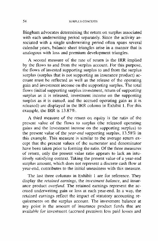
Year Paid to Nominal 2 Discounted 3 Supporting End Date Loss O/S Loss O/S Loss Surplus

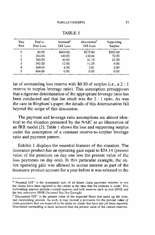
0 $0.00 $404.00 $375.86 $202.00 1 264.00 140.00 130.66 70.00 2 360.00 44.00 41.19 22.00 3 392.00 12.00 11.25 6.00 4 400.00 4.00 3.81 2.00 5 404.00 0.00 0.00 0.00

lar of outstanding loss reserve with $0.50 of surplus (i.e., a 2 : 1 reserve to surplus leverage ratio). This assumption presupposes that a rigorous determination of the appropriate leverage ratio has been conducted and that the result was the 2 : 1 ratio. As was the case in Bingham's paper, the details of this determination fall beyond the scope of this discussion.

The payment and leverage ratio assumptions are almost identical to the situation presented by the NAIC as an illustration of an IRR model [2]. Table 1 shows the loss and supporting surplus under the assumption of a constant reserve-to-surplus leverage ratio and payment pattern.

Exhibit 1 displays the essential features of the situation. The insurance product has an operating gain equal to $24.14 (present value of the premium on day one less the present value of the loss payments on day one). In this particular example, the entire operating gain was allowed to accrue interest as part of the insurance product account for a year before it was released to the

2"Nominal O/S" is the (estimated) sum of all future claim payments whether or not the claims have been reported to the carrier at the time that the estimate is made. This outstanding amount includes carried reserves and bulk reserves such as true IBNR and the less restrictive IBNE (Incurred But Not Enough). 3"Discounted O/S" is the present value of the expected flows that make up the nominal outstanding amount. As such, it may include a provision for the present value of claim payments that are expected to be made on claims that have not yet been reported. Discounted outstanding is more inclusive than the present value of the carried reserves.

52 SURPLUS CONCEPTS

surplus account. The accrued value of $24.14 after one year is $25.34.

Because the reserves along with their associated uncertainty remained constant during the first year, the supporting surplus was held constant at $202.00 for the entire year. The total return on this supporting surplus during the first year consisted of the $25.34 accrued operating gain from the insurance product and the $10.10 of investment income earned by the supporting surplus. The total, $35.44, represents a 17.55% return on the $202.00 surplus investment.

During subsequent years there was no contribution to the total return on supporting surplus arising from the insurance product. Investment income that was earned on underwriting funds during each calendar year was exactly sufficient to establish the year-end discounted loss reserve after all of the calendar year loss payments were made. In this respect, the insurance product did not participate in any further fund transfers between its own account and the surplus account after the end of the first year. Regardless of this, the fact that there was uncertainty regarding the ultimate loss outcome during each subsequent year led to the requirement that some surplus had to be allocated to the insurance product. During these subsequent years there was a 5% annual return on the supporting surplus. This is the same return as would have been earned had the surplus been idle (i.e., not supporting an insurance product). This surplus was, however, committed to supporting uncertainties during the runoff and was n o t available to support n e w writings. The average annual return on supporting surplus [E(released operating gain plus investment income on the supporting surplus)/E(supporting surplus), where the summation is over all years] was 13.39%.

It would not be correct to consider only the first year and to report a 17.55% return on equity for the product. Doing so would ignore the commitment of surplus during the subsequent four years. To see that this is precisely what is done when calendar year earnings are compared to average calendar

SURPLUS CONCEPTS 53

year surplus amounts, consider what the calendar year return would be if the carrier wrote only a single contract during its lifetime. The first year-end balance sheet would indicate an average surplus amount equal to $202.00, while the statement of income would reflect $35.44, giving us a 17.55% return on surplus for the calendar year.

It can be argued that a carrier 's calendar year return on equity would be equal to the average annual return on equity if the book of business were to be repeatedly renewed until a steady state had been achieved. Mathematically, this is a true statement. In the case of the single contract described above, repeated renewal for four or more years would result in an annual commitment of $302 of surplus ($202 for the most recently renewed contract, $70 for the contract written one year before, etc.) and annual income equal to $40.44 ($35.44 for the most recently renewed contract, $3.50 for the contract written one year before, etc.), which would yield a 13.39% return on supporting surplus for the calendar year.

Conceptually, the two measures are very different. While the average annual return measure relates to a single contract, the calendar year measure requires identical contracts to be written year after year. If the mix of business changes from year to year or if all of the company surplus is not being used to support the runoff of previously written contracts, then the equality no longer holds.

The conceptual difference between calendar year and average annual return on surplus is similar to the one that exists between accident year (or policy year) loss ratio and calendar year loss ratio. Here, too, the two measures are numerically equal once a steady state situation has been achieved. Each age to age development that is observed in the accident year (or policy year) triangle would be contributed to the calendar year experience by different accident year contracts in the corresponding stages of development. Just as one would not rely upon this equality when estimating the ultimate loss ratio for a single accident year,

54 SURPLUS CONCEPTS

Bingham advocates determining the return on surplus associated with each underwriting period separately. Since the activity associated with a single underwriting period often spans several calendar years, balance sheet triangles arise in a manner that is analogous with loss and premium development triangles.

A second measure of the rate of return is the IRR implied by the flows to and from the surplus account. For this purpose, the flows of invested supporting surplus to and from the surplus surplus (surplus that is not supporting an insurance product) account must be reflected as well as the release of the operating gain and investment income on the supporting surplus. The total flows (initial supporting surplus investment, return of supporting surplus as it is released, investment income on the supporting surplus as it is earned, and the accrued operating gain as it is released) are displayed in the IRR column in Exhibit 1. For this example, the IRR is 13.87%.

A third measure of the return on equity is the ratio of the present value of the flows to surplus (the released operating gains and the investment income on the supporting surplus) to the present value of the year-end supporting surplus, 13.58% in this example. This measure is similar to the average return ex- cept that the present values of the numerator and denominator have been taken prior to forming the ratio. Of the three measures of return, only the present value ratio appears to lack an intuitively satisfying context. Taking the present value of a year-end surplus amount, which does not represent a discrete cash flow at year-end, contributes to the initial uneasiness with this measure.

The last three columns in Exhibit 1 are for reference. They display the retained earnings, the investment balance, and insurance product overfund. The retained earnings represent the accrued underwriting gain or loss at each year-end. In a way, the retained earnings reflect the impact of statutory accounting requirements on the surplus account. The investment balance at any point is the amount of insurance product funds that are available for investment (accrued premium less paid losses and

SURPLUS CONCEPTS 55

released operating gain). The overfund is the amount by which the investment balance exceeds the discounted outstanding loss reserve. The overfund represents the portion of the operating gain that has been retained to act as an additional buffer against insolvency risk. No model is acceptable that does not come to an end with exactly zero overfund and zero investment balance. Any alternative to closing out the insurance product account after the last claim has been paid would result in allocating a portion of surplus to the insurance product (or floating it a loan) long after all claims had closed and all uncertainties had been resolved.

Exhibit 2 represents the same situation but with a withdrawal of operating gain at the opposite extreme from that which was depicted in Exhibit 1. In Exhibit 2, the operating gain is retained within the insurance product until all claims have been paid. As long as the operating gain is retained within the insurance product account, all interest accrued on it will be attributed to the insurance product. At the end of the fifth year, when the accrued operating gain is finally released to the surplus account, it carries with it $6.67 of accrued interest, all of which is considered as part of the total return on supporting surplus.

Once funds are released to the surplus surplus account, subsequent investment income earned by them is not attributed to the insurance product. Because the operating gain was released to the surplus account later than in Exhibit 1, more of the investment income earned on these funds was attributed to the insurance product ($6.67 vs. $1.20). As a result of the difference between these two arbitrary segregations of funds---between the insurance product account and surplus account-- the average annual return on supporting surplus increases from 13.39% as displayed in Exhibit 1 to 15.20% under the operating gain release timing of Exhibit 2. Whereas reflecting more dollars of investment income causes the average return on surplus to increase, it has the opposite effect on the IRR. The IRR corresponding to 13.87% of Exhibit 1 is 11.84% in Exhibit 2.

56 SURPLUS CONCEPTS

If the insurance company had set a 13.5% target for its return on equity and used these measures of return to evaluate this product, it would have found the product to fall short of the target if it had adopted the average return measure under the Exhibit 1 scenario, but to be acceptable under the Exhibit 2 scenario. Just the opposite conclusions would be reached if the IRR measures were used. Now, simply earmarking funds as belonging to a particular company account (insurance product account or surplus account) does not affect the overall well-being of the company. 4 There must be something misleading about a model that produces different results for different earmarkings. While the present value measure of the return on equity remained equal to 13.58% for both alternatives, invariance alone does not provide sufficient support for it to be adopted as the true measure of the return on equity.

Exhibit 3 provides that support. This example begins by spec- ifying how the operating gain is to be released to the surplus account. In this alternative, the operating gain is released Bing- ham's way, as uncertainty is resolved (i.e., under the same crite- ria that the supporting surplus is released). This timing results in releasing the operating gain in such a way that the ratio of released dollars to the invested surplus remains constant. In symbolic form, if S(j) is the invested surplus during the j th year, and O(j) is the accrued operating gain that is released at the end of the j th year, then the set {O(j)} must satisfy two conditions:

1. PV[{O(j)}] = the operating gain, and

2. O(j)/S(j) = constant for all years, independent of j .

The bottom of Exhibit 3 displays the detailed calculation of the set {O(j)} corresponding to this example.

4While actions taken as a result of this earmarking, such as the declaration of stockholder dividends, can affect the overall well-being of the company, the a c t of earmarking funds cannot affect the company's well-being.

SURPLUS CONCEPTS 57

As promised by Bingham, the three measures of the return on equity are equal when his release of operating gain is adopted. This is more than a coincidence. Appendix A presents a general proof that Condition 2 is sufficient to force the three measure- ments into agreement.

The invariant measure is equal to the average annual return on equity and to the internal rate of return corresponding to the case in which operating earnings are released in the same manner as supporting surplus, as uncertainty is resolved. The invariant measure does have a context.

It should be emphasized that the only feature of the insurance product cash flow that is explicitly reflected in the determination of the return on surplus is the present value of the operating gain. Increasing the degree of sophistication of the insurance product model (e.g., reflecting federal income tax, other expenses, policyholder dividends, etc.) almost certainly will change the numerical value of the operating gain but will not alter any of the concepts that have been discussed. Once the operating gain is determined, the manner in which it is released remains unchanged (i.e., ac- cording to the two conditions), and the agreement among the IRR, average annual return, and the model invariant continues to hold.

3. DOES THE BINGHAM METHODOLOGY LEAD TO REASONABLE

RESULTS?

All of the exhibits thus far have been based upon a situation that generates an operating profit. Furthermore, while the Bing- ham invariant ratio, average annual return on equity, and internal rate of return produce different measures of the return on equity, they do not differ significantly in the absence of the Bingham release scheme. For the purpose of a reasonableness check, a new example will be presented. The longer payout period accentuates the differences between the three measures of ROE when the

58 SURPLUS CONCEPTS

T A B L E 2

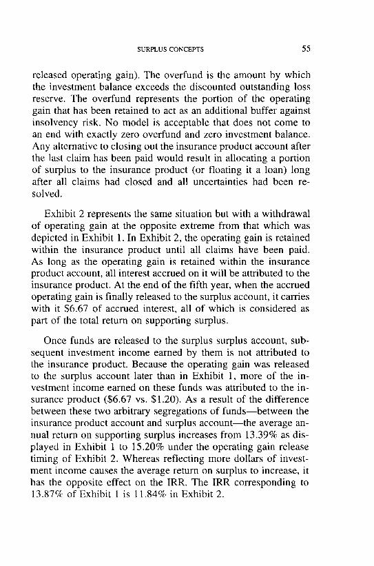
E L E M E N T S C O M M O N TO E X H I B I T S 4-6

Year Paid to Nominal Discounted Supporting Required End Date Loss O/S Loss O/S Loss Surplus Funds

0 $0.00 $2,000.00 $961.38 $1,000.00 $1,961.38 1 0.00 2,000.00 1,009.45 1,000.00 2,009.45 2 0.00 2,000.00 1,059.92 1,000.00 2,059.92 3 6.00 1,994.00 1,106.92 997.00 2,103.92 4 34.00 1,966.00 1,134.26 983.00 2,117.26 5 120.00 1,880.00 1,104.98 940.00 2,044.98 6 184.00 1,816.00 1,096.23 908.00 2,004.23 7 258.00 1,742.00 1,077.04 871.00 1,948.04 8 332.00 1,668.00 1,056.89 834.00 1,890.89 9 404.00 1,596.00 1,037.73 798.00 1,835.73

10 474.00 1,526.00 1,019.02 763.00 1,782.62 11 526.00 1,474.00 1,018.60 737.00 1,755.60 12 574.00 1,426.00 1,021.53 713.00 1,734.53 13 618.00 1,382.00 1,028.61 691.00 1,719.61 14 660.00 1,340.00 1,038.04 670.00 1,708.04 15 693.00 1,304.00 1,053.94 652.00 1,705.94 16 730.00 1,270.00 1,072.64 635.00 1,707.64 17 760.00 1,240.00 1,096.27 620.00 1,716.27 18 788.00 1,212.00 1,123.08 606.00 1,729.08 19 1,312.00 688.00 655.24 344.00 999.24 20 2,000.00 0.00 0.00 0.00 0.00

release of operating gain does not follow the resolution of uncertainty.

The longer payout period of this example is similar to that of high attachment point workers compensation excess of loss reinsurance. By the end of the 18th year, less than 40% of the ultimate loss is expected to have been paid. Table 2 displays the elements that are common to Exhibits 4 through 6.

The Required Funds column consists of the funds that must be allocated to the insurance product, an amount equal to the discounted outstanding loss plus the supporting surplus. Any additional funds may be released to the surplus account at any time.

SURPLUS CONCEPTS 59

The reasonableness check begins with a simple observation. If the operating gain associated with the insurance product is exactly zero (i.e., the premium is just sufficient to fund the discounted loss reserves), then there can be no net flow from the insurance product to or from the surplus account. Supporting surplus must be allocated, but all that can be earned on the supporting surplus is the 5% return that could be earned on idle surplus. No release of the operating gain (i.e., a set of non-zero flows that have a present value equal to zero) that results in a return on equity other than 5% is reasonable.

Exhibits 4A and 4B present just such a zero operating gain situation. With $961.38 of premium and $2,000 of expected loss, the underwriting loss would be $1,038.62 and the incurred loss ratio would be 208%. A premium equal to $961.38, paid on day one, exactly funds the discounted outstanding loss reserve. With no funds to spare, the operating gain is exactly zero. While supporting surplus is required during the 20 year runoff, its return will be exactly the same as if the insurance product had not been written, 5%. No measurement of the return on surplus other than 5% would be reasonable for this situation.

A quick glance at Exhibit 4A discloses that Bingham's invariant ratio passes the test, whereas the average annual return, at 8.1%, clearly fails the test.

The rather peculiar looking release of operating gain, {O(j)}, mimics the requirements of statutory accounting (SAP). Under SAP, the carrier must fund the nominal reserves rather than the discounted reserves. As a result of this requirement, the $961.38 premium falls short by $1,038.62. Consistent with the SAP requirement, $1,038.62 must be transferred from surplus surplus to the product on day one. The equivalent year-end transfer is displayed on Exhibit 4A. The $990.55 transfer can be thought of as the day one transfer of $1,038.62 plus interest (totaling $51.93) less the interest earned on the $2,000 nominal reserve (a total of $100.00).

60 SURPLUS CONCEPTS

While this set of operating gain flows is allowable (their present value is zero and they produce a zero investment balance by the end of the 20 year runoff), the corresponding 8.1% average annual return on supporting surplus is, clearly, unreasonable. This paradoxical result is an example of the type of manipulation that Bingham's release scheme is designed to prevent.

This manipulation was previously encountered in the first example for which the operating gain was greater than zero and for which all flows were positive. In that example, it was noted that once a flow is released to the surplus account, no further investment income earned on this money is credited to the insurance product. The longer the operating gain is retained as part of the insurance product, the more of its earned investment income is credited to the insurance product. Interest earned on surplus surplus is ignored, regardless of its source.

Likewise, when some of the flows are negative, the interest that is not earned (lost) by the surplus surplus is ignored. The insurance product, rather than surplus surplus, receives credit for the earned investment income. The $485.65 of nominal gain (sum of the stream of O(j) flows) that appears to have been generated by the insurance product was at the (unrecognized) expense of the surplus surplus account.

If the average annual return on surplus is viewed as being the calendar year return once a steady state situation has been achieved, then the identification of the source of the additional $485.65 return is somewhat different. Under a steady state interpretation, the flows from year-ends 1 through 20 represent the contribution of previously written policies to the current calendar year. Under this interpretation, the policies in runoff do provide sufficient funds to establish the initial reserve on newly written policies and provide the missing 3.1% return on the steady state supporting surplus. What is missing in this interpretation is the cost of establishing the steady state (transferring funds from surplus to establish the first twenty years of writings). The additional 3.1% return is exactly equal to the investment income

SURPLUS CONCEPTS 61

being lost by the surplus surplus account as a result of funding the underwriting loss for the first 20 years.

The final columns of Exhibit 4A display the calendar year return on equity during each year, if the SAP release scheme were to be followed. During the first 20 years, the runoff from succes- sively more accident years is reflected in each annual statement. Eventually by year 20, the statement ROE reflects one year-end ROE for each of the 20 accident years. Growth from year to year affects the relative amount of each maturity that is reflected in the year-end ROE. Only when the exposure growth rate is 5% does the calendar year ROE approach the reasonable 5% figure.

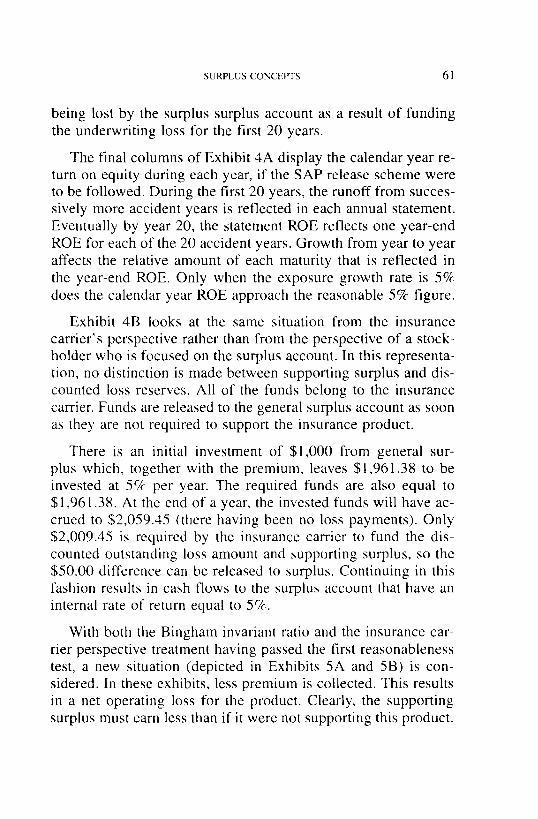
Exhibit 4B looks at the same situation from the insurance carrier 's perspective rather than from the perspective of a stockholder who is focused on the surplus account. In this representa- tion, no distinction is made between supporting surplus and discounted loss reserves. All of the funds belong to the insurance carrier. Funds are released to the general surplus account as soon as they are not required to support the insurance product.

There is an initial investment of $1,000 from general surplus which, together with the premium, leaves $1,961.38 to be invested at 5% per year. The required funds are also equal to $1,961.38. At the end of a year, the invested funds will have accrued to $2,059.45 (there having been no loss payments). Only $2,009.45 is required by the insurance carrier to fund the discounted outstanding loss amount and supporting surplus, so the $50.00 difference can be released to surplus. Continuing in this fashion results in cash flows to the surplus account that have an internal rate of return equal to 5%.

With both the Bingham invariant ratio and the insurance carrier perspective treatment having passed the first reasonableness test, a new situation (depicted in Exhibits 5A and 5B) is considered. In these exhibits, less premium is collected. This results in a net operating loss for the product. Clearly, the supporting surplus must earn less than if it were not supporting this product.

62 SURPLUS CONCEPTS

As can be seen in Exhibit 5A, Bingham's invariant ratio represents a reasonable measure of the return on surplus; it is less than that of idle surplus. The statutory accounting model, again, fails the test because its ROE is greater than that of idle surplus.

From the insurance carrier's perspective (Exhibit 5B), $1,961.38 is required to support the product, but only $600.00 is received in the form of premium. The additional $1,361.38 must be supplied from the surplus account. While not produc- ing the same ROE as Bingham's scheme does, this measure is reasonable.

Both the Bingham scheme and the insurance carrier perspective agree that surplus would increase faster if this product, with its 333% loss ratio, were not written. The statutory accounting model does not agree.

A reasonable model should report an ROE that is greater than that of idle surplus if there is an operating gain produced by the insurance product. The purpose of supporting surplus is to cushion against uncertainty. If the premium is sufficient to fund the discounted loss reserve for the expected losses and to provide the required cushion against uncertainty, then no contribution of supporting surplus should be required. As the premium ap- proaches this "no risk to the carrier" amount, the ROE should increase without bound. This expectation provides another test of a model 's behavior.

Exhibit 6A displays the first portion of the reasonableness test when there is a net operating profit. With $1,700 of premium, there is a $738.62 operating gain. All three measures of ROE are greater than that of idle surplus (5%).

Both Bingham and the statutory model allocate the same amount of supporting surplus that they did in the other two cases. From the insurance carrier perspective (Exhibit 6B), only $261.38 of surplus is needed in addition to the premium in order to fully fund the discounted outstanding loss and supply the required amount of cushion against uncertainty.

SURPLUS CONCEPTS 63

TABLE 3

RETURN ON EQUITY FOR EACH MEASURE

Premium

Bingham Insurance Operating Loss SAP Invariant Cartier IRR

Gain Ratio Measure Measure Measure

$ 500.00 $ - 461.38 400.0% 5.0% 0.6% 1.6% 600.00 -361.38 333.3% 5.7% i.5% 2.2% 700.00 -261.38 285.7% 6.3% 2.5% 2.9% 800.00 -161.38 250.0% 7.0% 3.4% 3.6% 900.00 -61.38 222.2% 7.7% 4.4% 4.4% 961.38 0.00 208.0% 8.1% 5.0% 5.0%

1,000.00 38.62 200.0% 8.3% 5.4% 5.4% 1,100.00 138.62 181.8% 9.0% 6.3% 6.5% 1,200.00 238.62 166.7% 9.7% 7.3% 7.8% 1,300.00 338.62 153.8% 10.3% 8.3% 9.4% 1,400.00 438.62 142.9% 11.0% 9.2% 11.4% 1,500.00 538.62 133.3% 11.7% 10.2% 14.1% 1,600.00 638.62 125.0% 12.3% 11.1% 18.0% 1,700.00 738.62 117.6% 13.0% 12.1% 24.4% 1,800.00 838.62 111.1% 13.7% 13.1% 37.5% 1,900.00 938.62 105.3% 14.3% 14.0% 88.3% 1,920.00 958.62 104.2% 14.5% 14.2% 126.6% 1,940.00 978.62 103.1% 14.6% 14.4% 237.3% 1,950.00 988.62 102.6% 14.7% 14.5% 441.1% 1,960.00 998.62 102.0% 14.7% 14.6% 3,620.8%

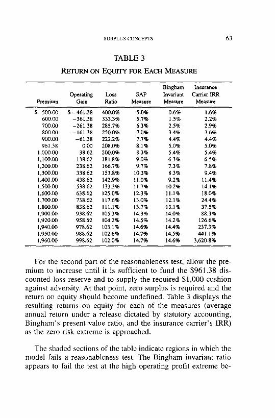
For the second part of the reasonableness test, allow the premium to increase until it is sufficient to fund the $961.38 discounted loss reserve and to supply the required $1,000 cushion against adversity. At that point, zero surplus is required and the return on equity should become undefined. Table 3 displays the resulting returns on equity for each of the measures (average annual return under a release dictated by statutory accounting, Bingham's present value ratio, and the insurance carrier's IRR) as the zero risk extreme is approached.

The shaded sections of the table indicate regions in which the model fails a reasonableness test. The Bingham invariant ratio appears to fail the test at the high operating profit extreme be-

64 SURPLUS CONCEFI'S

cause the required supporting surplus does not reflect the fact that the retained operating funds provide an additional (unquantified) cushion against uncertainty.

If the required surplus were to be reduced in recognition of the retained operating gain, with the sum of the supporting surplus and retained operating gain providing the required cushion (at a 2 : 1 reserve to cushion ratio), then insurance products with a larger expected operating gain would require less surplus. As the expected operating gain approached the required cushion amount, the required surplus would approach zero, and the re- suiting return on surplus would increase without bound as the expected operating gain approached this no risk situation.

Were it not for the Bingham requirement that the operating gain be released so as to maintain a constant return on the supporting surplus, reducing the surplus in recognition of the retained operating gain would be a trivial exercise. Difficulty arises because the set of release flows, {O(j)}, depends upon the year- end surplus amounts, {S(j)), which in turn depend upon the set of retained operating gains, {R(j)}. These retained gains depend upon what has been previously released, the set {O(j)).

Attempting to find a set of flows and surplus amounts that satisfy the two relations,

O ( j ) / S ( j - 1) = k, independent of j, and

R(j) + S(j) = Reserves at year-end j divided by the reserves-to-cushion ratio

is not a trivial matter.

Solving this linked set of equations in closed form requires solving a polynomial of degree 20 for a product with a 20 year runoff. 5 Attempting to solve the system by an iterative technique

5The polynomial arises as the result of an attempt to determine the operating gain to be released at each year-end. As demonstrated in Appendix A, in the absence of modifying the supporting surplus to reflect the cushioning effect of the retained operating gain, a set

SURPLUS CONCEPTS 65

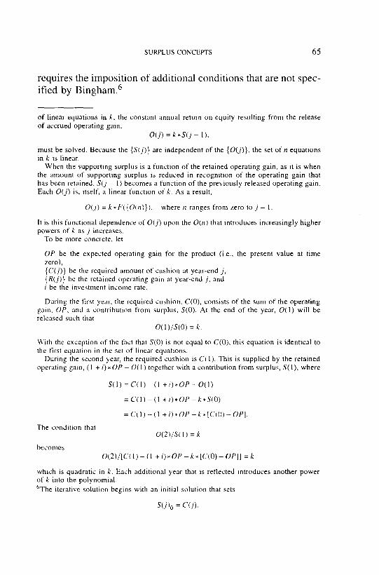
requires the imposition of additional conditions that are not spec- ified by Bingham. 6

of linear equations in k, the constant annual return on equity resulting from the release of accrued operating gain,

O ( j ) = k ,~ S ( j - I),

must be solved. Because the {S(j)} are independent of the {O(j)}, the set of n equations in k is linear.

When the supporting surplus is a function of the retained operating gain, as it is when the amount of supporting surplus is reduced in recognition of the operating gain that has been retained, S ( j - 1 ) becomes a function of the previously released operating gain. Each O ( j ) is, itself, a linear function of k. As a result,

O ( j ) = k * F ( { O ( n ) } ) , w h e r e n ranges from zero to j - 1 .

It is this functional dependence of O ( j ) upon the O(n) that introduces increasingly higher powers of k as j increases.

To be more concrete, let

O P be the expected operating gain for the product (i.e., the present value at time zero), {C(j)} be the required amount of cushion at year-end j , {R(j)} be the retained operating gain at year-end j , and i be the investment income rate.

During the first )'ear, the required cushion, C(O), consists of the sum of the operating gain, O P , and a contribution from surplus, S(O). At the end of the year, 0 (1) will be released such that

o ( 1 ) / s ( o ) = k.

With the exception of the fact that S(0) is not equal to C(0), this equation is identical to the first equation in the set of linear equations.

During the second year, the required cushion is C( 1 ). This is supplied by the retained operating gain, (1 + i)* O P - O(1) together with a contribution from surplus, S(I), where

The condition that

becomes

S(I) = C ( I ) - ( I + i ) * O P - O ( l )

= C ( I ) - ( 1 + i ) * O P - k * S ( O )

= C ( l ) - ( I + i ) * O P - k * [ C ( O ) - O P ] .

0 ( 2 ) / S ( 1 ) = k

0 ( 2 ) / [ C ~ l) - ( l + i)* O P - ~ * [C(0) - OP]] = k

which is quadratic in k. Each additional year that is reflected introduces another power of k into the polynomial. 6The iterative solution begins with an initial solution that sets

S(j) 0 = C~)).

66 SURPLUS CONCEPTS

4. R E F I N E M E N T S T O T H E B I N G H A M M E T H O D O L O G Y I

( N O M I N A L VS. D I S C O U N T E D R E S E R V E S )

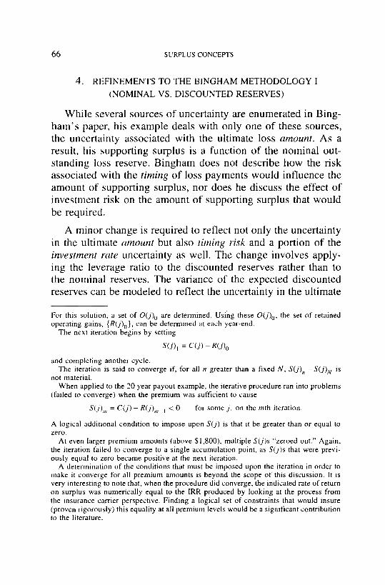
While several sources of uncertainty are enumerated in Bing- ham's paper, his example deals with only one of these sources, the uncertainty associated with the ultimate loss amount. As a result, his supporting surplus is a function of the nominal outstanding loss reserve. Bingham does not describe how the risk associated with the timing of loss payments would influence the amount of supporting surplus, nor does he discuss the effect of investment risk on the amount of supporting surplus that would be required.

A minor change is required to reflect not only the uncertainty in the ultimate amount but also timing risk and a portion of the investment rate uncertainty as well. The change involves apply- ing the leverage ratio to the discounted reserves rather than to the nominal reserves. The variance of the expected discounted reserves can be modeled to reflect the uncertainty in the ultimate

For this solution, a set of O ( j ) o are determined. Using these O(j) 0, the set o f retained operating gains, {R(J)0}, can be determined at each year-end.

The next iteration begins by setting

S(j) 1 = C ( j ) - R ( j ) o

and completing another cycle. The iteration is said to converge it', for all n greater than a fixed N, S ( j ) . - S ( j ) N is

not material. When applied to the 20 year payout example, the iterative procedure ran into problems

(failed to converge) when the premium was sufficient to cause

S(j),,, = C ( j ) - R( j ) , . I < 0 for some j , on the ruth iteration.

A logical additional condition to impose upon S ( j ) is that it be greater than or equal to zero.

At even larger premium amounts (above $1,800), multiple S(j)s "zeroed out." Again, the iteration failed to converge to a single accumulation point, as S(j)s that were previously equal to zero became positive at the next iteration.

A determination of the conditions that must be imposed upon the iteration in order to make it converge for all premium amounts is beyond the scope of this discussion. It is very interesting to note that, when the procedure did converge, the indicated rate of return on surplus was numerically equal to the IRR produced by looking at the process from the insurance carrier perspective. Finding a logical set of constraints that would insure (proven rigorously) this equality at all premium levels would be a significant contribution to the literature.

SURPLUS CONCEPTS 67

amount, uncertainty in the cash flow timing, and uncertainty in the investment income rate as well. A description of how one would determine the leverage ratio that would cushion against variation of the expected discounted reserve around its mean is beyond the scope of this discussion.

When the role of the cushion is restricted to covering the ul- t imate amount at risk, it is still appropriate to apply a leverage ratio to discounted reserves. Even if the actual future loss payments are greater than expected, only the present value of the unexpected payments needs to be available now. It will accrue to the required amount by the time it must be used.

Returning to the original example, the nominal loss reserve is $44.00 at the end of year two. The 2 : 1 reserve to surplus ratio 7 implies that if $66.00 is made available to pay losses ($44.00 of loss reserve and $22.00 of supporting surplus), then the probability of ruin can be kept below some pre-established amount (e.g., less than 0.02). If there is no uncertainty regarding the timing of the future payments (i.e., the percentages of the actual ultimate loss to be paid by each year end are exactly those which were expected), then each future loss payment will be 50% higher than expected in this worst case scenario. If the $41.19 discounted loss reserve accrues to pay the expected future losses, then an additional $20.60 (50% of the discounted outstanding loss amount) should be sufficient to make the unexpected payments if they become due.

Differences between the expected and actual timing of loss payments have no impact upon the nominal loss reserves that should be carried but do affect the amount of discounted loss reserve that should be carried at any point in time. It is logical to cushion against the timing uncertainty that increases the

71t has been assumed that the original 2 : 1 leverage ratio does not reflect any implicit discounting for interest.

68 SURPLUS CONCEPTS

variance in the discounted loss reserve by adopting the discounted reserve as the surplus allocation base.

5. REFINEMENTS TO THE BINGHAM METHODOLOGY II

(A DECREASING LEVERAGE RATIO)

Bingham assumes that a constant reserve-to-surplus leverage ratio results when supporting surplus is established to maintain a constant probability of ruin. While this assumption is consistent with the other simplifications that he adopted for illustrative purposes, it must be emphasized that it is neither required to achieve an invariant ratio, nor is it realistic. Many models that allocate surplus over the life of a product assume that a constant leverage ratio is appropriate. Some models even allow the leverage ratio to increase over time. For many circumstances, the leverage ratio must decrease over the long run if a constant probability of ruin is to be maintained. This is not to say that a short term increase in the ratio of reserves to surplus is impos- sible, but that such a short term increase will be followed by a long term decrease as the runoff becomes increasingly more volatile.

For illustrative purposes, consider the hypothetical case of excess of loss casualty reinsurance with a very high attachment point. Because of the high attachment point, assume that small claims will be eliminated. Assume, further, that those claims that remain can be modeled by one of the more common distributions (e.g., the lognormal or Pareto distribution). A suitably high attachment point assures us that all of the possible claims will fall in the relatively flat tail o f the severity distribution. This means that the likelihood of any particular claim size is almost equal to that of any other size claim. If each claim closes with a single payment and this payment does not depend upon how long the claim remained open before being settled, then the ultimate closing amount on each open claim can be represented by a stochas-

SURPLUS CONCEVFS 69

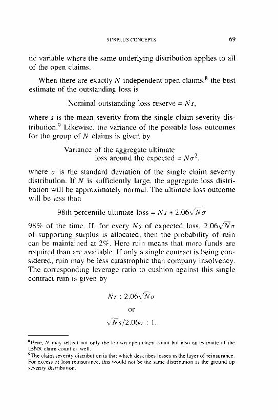
tic variable where the same underlying distribution applies to all of the open claims.

When there are exactly N independent open claims, 8 the best estimate of the outstanding loss is

Nominal outstanding loss reserve = Ns,

where s is the mean severity from the single claim severity dis-

tribution. 9 Likewise, the variance of the possible loss outcomes for the group of N claims is given by

Variance of the aggregate ultimate loss around the expected = No -2,

where o- is the standard deviation of the single claim severity distribution. If N is sufficiently large, the aggregate loss distribution will be approximately normal. The ultimate loss outcome will be less than

98th percentile ultimate loss = Ns + 2.06v/~/o-

98% of the time. If, for every Ns of expected loss, 2.06v/No- of supporting surplus is allocated, then the probability of ruin can be maintained at 2%. Here ruin means that more funds are required than are available. If only a single contract is being considered, ruin may be less catastrophic than company insolvency. The corresponding leverage ratio to cushion against this single contract ruin is given by

Ns " 2.{)6V~o-

o r

v~s/2 .06o-" 1.

8Here, N may reflect not only the known open claim count but also an estimate of the IBNR claim count as well. 9The claim severity distribution is that which describes losses in the layer of reinsurance. For excess of loss reinsurance, this would not be the same distribution as the ground up severity distribution.

70 SURPLUS CONCEPTS

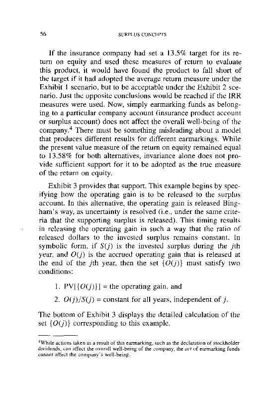
TABLE 4

Year Paid to Nominal Discounted Leverage Supporting End Date Loss O/S Loss O/S Loss Ratio Surplus

0 $0.00 $404.00 $375.86 2.00 : 1.00 $187.93 1 264,00 140.00 130.66 1.18 : 1.00 110.97 2 360.00 44.00 41.19 0.66 : 1,00 62.40 3 392.00 12.00 11.25 0.34 : 1.00 32.63 4 400.00 4.00 3.81 0.20 : 1.00 19.14 5 404,00 0.00 0.00 N/A 0,00

As claims close, N, the number of open claims, decreases. As shown above, the leverage decreases in proportion to the square root of N.

If there are insufficient open claims to warrant the normal approximation, then the 98th percentile would have to be determined by means of some other aggregate loss modeling technique. The important point is that as the number of open claims decreases, the relative uncertainty increases as a function of the expected loss amount. In other words, the absolute amount of surplus may decrease, but the relative amount increases.

If claims are closed with a single payment and the same severity distribution can represent each claim, then the percentage of ultimate loss that is paid at any point in time is a measure of the number of claims that have been paid. Assuming that a 2 : 1 reserve-to-surplus ratio is appropriate at time zero, when none of the claims are closed, then the appropriate reserve-to- surplus ratio would become 2v@5 • 1 when 25% of the claims have closed. Returning to the original example with a five year runoff, and introducing both the modified leverage ratio and the discounted outstanding loss reserve as the base, the supporting surplus amounts shown in Table 4 are required at each year- end.

The initial supporting surplus, $187.93, is less than the $202.00 of supporting surplus for the unmodified case. This

SURPLUS CONCEPTS 71

quickly changes as the leverage ratio decreases (i.e., more surplus is required to support a dollar of loss reserve as the number of open claims decreases and the proportionate volatility increases) and the offsetting loss discount unwinds.

Exhibit 7 displays the correspondingly modified Bingham model. Notice that the average return on surplus and internal rate of return remain equal to the Bingham invariant ratio after the modification. Because the modification involves changing the amount of supporting surplus, the invariant ratio is not equal to the corresponding invariant ratio displayed on the other exhibits. Such agreement would not be expected.

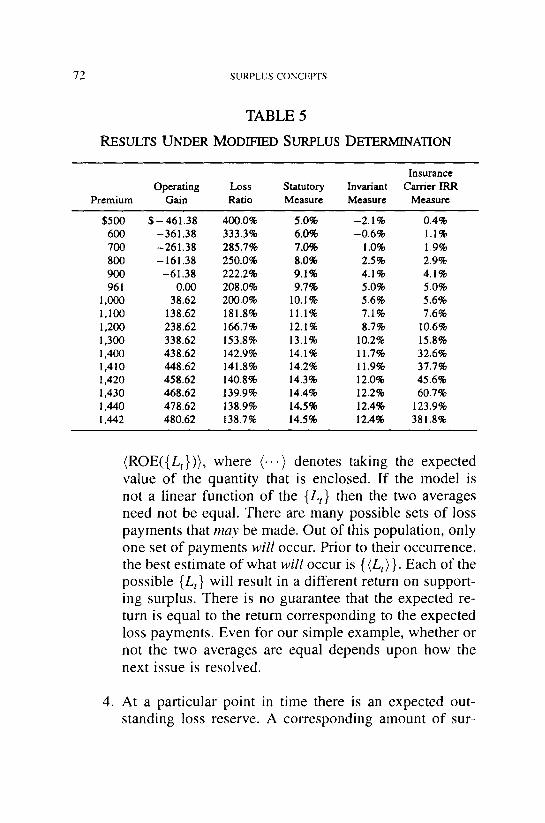
Exhibits 8A and 8B apply the modifications to the second example. While the invariant ratio is numerically equal to the internal rate of return from the perspective of the insurance carrier, this is simply a coincidence produced by rounding errors. Table 5 provides a comparison of the three models under the modified surplus determination.

6. OTHER ISSUES

There are a number of issues that fall outside the scope of this discussion paper. They are briefly mentioned in the hope that they may encourage further discussion.

1. How can the other sources of insurance product uncertainty be reflected?

2. How can the appropriate leverage ratios for a selected probability of ruin be determined empirically?

. As presented, the model produces a point estimate of the return on equity. Expected loss amounts and payout timing are all that have been reflected in the determination of the return on equity. If {Lt} represents the actual loss payments at times {t}, then the return on equity that has been determined is ROE({ (Lt)}) rather than

72 SURPLUS CONCEPTS

TABLE 5

R E S U L T S U N D E R M O D I F I E D S U R P L U S D E T E R M I N A T I O N

Insurance Operating Loss Statutory Invariant Cal-rier IRR

Premium Gain Ratio Measure Measure Measure

$500 $ - 4 6 1 . 3 8 400.0% 5.0% -2 .1% 0.4% 600 -361.38 333.3% 6.0% -0 .6% 1.1% 700 -261.38 285.7% 7.0% 1.0% 1.9% 800 -161.38 250.0% 8.0% 2.5% 2.9% 900 -61.38 222.2% 9.1% 4.1% 4.1% 961 0.00 208.0% 9.7% 5.0% 5.0%

1,000 38.62 200.0% 10.1% 5.6% 5.6% 1,I00 138.62 181.8% 11.1% 7.1% 7.6% 1,200 238.62 166.7% 12.1% 8.7% 10.6% 1,300 338.62 153.8% 13.1% 10.2% 15.8% 1,400 438.62 142.9% 14.1% 11.7% 32.6% 1,410 448.62 141.8% 14.2% 11.9% 37.7% 1,420 458.62 140.8% 14.3% 12.0% 45.6% 1,430 468.62 139.9% 14.4% 12.2% 60.7% 1,440 478.62 138.9% 14.5% 12.4% 123.9% 1,442 480.62 138.7% 14.5% 12.4% 381.8%

(ROE({Lt})), where ( . . . ) denotes taking the expected value of the quantity that is enclosed. If the model is not a linear function of the {Lt} then the two averages need not be equal. There are many possible sets of loss payments that may be made. Out of this population, only one set of payments will occur. Prior to their occurrence, the best estimate of what will occur is {{Lt) }. Each of the possible {Lz} will result in a different return on supporting surplus. There is no guarantee that the expected return is equal to the return corresponding to the expected loss payments. Even for our simple example, whether or not the two averages are equal depends upon how the next issue is resolved.

4. At a particular point in time there is an expected outstanding loss reserve. A corresponding amount of sur-

SURPLUS CONCEPTS 73

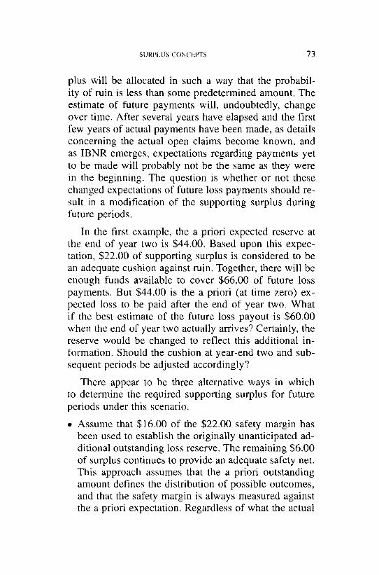
plus will be allocated in such a way that the probability of ruin is less than some predetermined amount. The estimate of future payments will, undoubtedly, change over time. After several years have elapsed and the first few years of actual payments have been made, as details concerning the actual open claims become known, and as IBNR emerges, expectations regarding payments yet to be made will probably not be the same as they were in the beginning. The question is whether or not these changed expectations of future loss payments should result in a modification of the supporting surplus during future periods.

In the first example, the a priori expected reserve at the end of year two is $44.00. Based upon this expectation, $22.00 of supporting surplus is considered to be an adequate cushion against ruin. Together, there will be enough funds available to cover $66.00 of future loss payments. But $44.00 is the a priori (at time zero) expected loss to be paid after the end of year two. What if the best estimate of the future loss payout is $60.00 when the end of year two actually arrives? Certainly, the reserve would be changed to reflect this additional information. Should the cushion at year-end two and subsequent periods be adjusted accordingly?

There appear to be three alternative ways in which to determine the required supporting surplus for future periods under this scenario.

• Assume that $16.00 of the $22.00 safety margin has been used to establish the originally unanticipated additional outstanding loss reserve. The remaining $6.00 of surplus continues to provide an adequate safety net. This approach assumes that the a priori outstanding amount defines the distribution of possible outcomes, and that the safety margin is always measured against the a priori expectation. Regardless of what the actual

74 SURPLUS CONCEPTS

estimate is, the supporting surplus cushions against the a priori estimate of the worst case scenario. Under this alternative, all differences between the expected values and the actual values are attributed to process variance. There is no cushion provided for parameter errors contained in the a priori expectations.

In a sense, this method is analogous to a loss ratio reserving methodology in which IBNR reserves are established equal to the difference between the a priori loss ratio and the reported loss ratio. Only if the difference becomes negative (i.e., reported amounts exceed expected amounts) is the a priori assumption ques- tioned. A negative difference means that ruin has occurred.

Assume that the a priori outstanding loss amount defines the size of the uncertainty, $22.00. Even when year two ends and the outstanding loss estimate (and it is still just an estimate as of year-end two) is $60.00 rather than the expected $44.00, $22.00 of surplus provides the necessary safety margin.

This alternative is analogous to the Bornhuet- ter/Ferguson loss reserving methodology. Future development (and uncertainty) depends upon an a priori assumption which is not modified to reflect current information.

Assume that the $60.00 estimate contains the same percentage of uncertainty as did the $44.00 a priori estimate. In this case, the supporting surplus must be increased from $22.00 to $30.00. Intuitively, this approach is less than satisfying because it appears to imply that the claim department 's opinion at the end of year two not only does nothing to decrease the uncertainty over the a priori estimate that was available at the beginning of year zero but actually increases the dollar amount of uncertainty. This alternative assumes

SURPLUS CONCEPTS 75

that the a priori estimate was based upon so much parameter error as to be worthless once additional information becomes available.

This alternative is analogous to the chain ladder reserving methodology which is 100% responsive to the current information.

A resolution of how to deal with actual estimates vs. a priori expectations will be necessary in order to determine whether or not the point estimate, ROE({ (Lt)}), will be equal to the ensemble average (i.e., ROE({Lt}) run for each of the {Lt} and then weighted by the probability of occurrence), (ROE({Lt})). If the two estimates are not equal, then even a prospective evaluation of the rate of return must be performed on an ensemble of possible insurance product outcomes rather than a single expected value outcome.

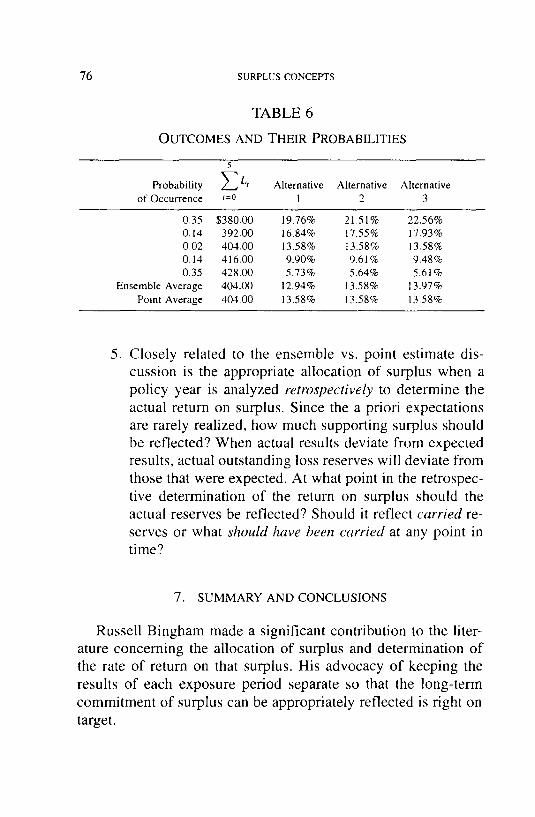
For our simple example, the second alternative results in a linear model whereas the other two do not. This can easily be demonstrated by running several possible loss outcomes through the Bingham model. The expected loss for the example is $404.00. Without changing the payout pattern (i.e., the percentage of ultimate loss paid at any particular point in time), consider Table 6, the possible loss outcomes and their corresponding probabilities of occurrence.

Note that Alternatives 1 and 3 produce deviations from the point estimate that are in opposite directions. The more volatile the loss distribution (the larger the variance), the more pronounced the deviation between the ensemble and point estimates will be for non-linear models.

While tinearity makes the calculations easier, compu- tational difficulty should not be the only criterion that is used in the selection of an alternative.

76 S U R P L U S C O N C E P T S

TABLE 6

O U T C O M E S A N D T H E I R P R O B A B I L I T I E S

5

Probability Z Lr Alternative Alternative Alternative of Occurrence t=o 1 2 3

0,35 $380.00 19.76% 21,51% 22.56% 0.14 392.00 16.84% 17.55% 17.93% 0.02 404.00 13.58% t3.58% 13.58% 0.14 416.00 9.90% 9.61% 9.48% 0.35 428.00 5.73% 5.64% 5.61%

Ensemble Average 404.00 12.94% 13.58% 13,97% Point Average 404.00 13.58% 13.58% 13.58%

, Closely related to the ensemble vs. point estimate discussion is the appropriate allocation of surplus when a policy year is analyzed retrospectively to determine the actual return on surplus. Since the a priori expectations are rarely realized, how much supporting surplus should be reflected? When actual results deviate from expected results, actual outstanding loss reserves will deviate from those that were expected. At what point in the retrospective determination of the return on surplus should the actual reserves be reflected? Should it reflect carried reserves or what should have been carried at any point in time?

7. S U M M A R Y A N D C O N C L U S I O N S

Russell Bingham made a significant contribution to the literature concerning the allocation of surplus and determination of the rate of return on that surplus. His advocacy of keeping the results of each exposure period separate so that the long-term commitment of surplus can be appropriately reflected is fight on target.

SURPLUS CONCEPTS 77

In the process of taking the present values of the insurance flows and supporting surplus, Bingham has produced an invariant measure of the return on surplus.

The difference between the commonly used calendar year determination of the return on surplus and Bingham' s accident year approach can be illustrated by the following two descriptions of the same investment:

• Calendar Year Approach: A carrier invests $1,000 of surplus and receives a $400 return, so the return on surplus is 40%;

• Accident Year Approach: A carrier invests $1,000 of surplus for 10 years and receives an average annual return equal to 3.4% on its investment.

The second approach takes into account the time over which the surplus funds are invested (until all of the uncertainties are resolved). This time horizon is well beyond the time that premiums are in force for most insurance products.

If a given probability of ruin is to be maintained by cushioning funds, then there must be some recognition of the cushion afforded by the premium provision for expected operating profit. Otherwise, the probability of ruin will vary with premium in a manner that is difficult to rationalize. This would appear to imply that ruin occurs whenever the expected operating profit is not achieved rather than whenever there are insufficient funds to meet the unexpected losses and expenses. The latter definition seems to be a more logical way to define ruin. This is an area that warrants further investigation.

Two modifications that can be made to enhance Bingham's model have been proposed. In actual practice, the leverage ratio will vary, but not in such a simple manner as suggested by the square root rule. A more detailed investigation of the character- istics of a particular line must be undertaken in order to establish actual leverage ratios for the runoff of a maturing policy year.

78 SURPLUS CONCEPTS

While not exhaustive, a list of additional considerations provides issues that must be addressed. In particular, the idea of av- eraging the returns over an ensemble of possible loss outcomes forces us to refine our ideas concerning the role of surplus as it cushions against ruin.

SURPLUS CONCEPTS 79

REFERENCES

[ 1] Heckman, Philip E. and Glenn G. Meyers, "The Calculation of Aggregate Loss Distributions from Claim Severity and Claim Count Distributions," PCAS LXX, 1983, pp. 22-71.

[2] N.A.I.C. Study of Investment Income, Supplement to the Proceedings, National Association of Insurance Commis- sioners, 1984, Vol. II, pp. 504-507.

[3] The Workers Compensation Rating and Inspection Bureau of Massachusetts, Filing for rates to become effective January 1, 1988, p. 701.

0~ O

EXHIBIT 1

A NOT COMPLETELY BINGHAM MODEL

INSURANCE PRODUCT SURPLUS ACCOUNT IRR INSURANCE PRODUCT

Idle Idle Total O(n) =~ Supporting Funds Surplus Surplus Return on Total

End of Written Paid Operating Funds Surplus Released Investment Investment Supporting Surplus Retained Investment Year Premium Loss Gain Released S to Surplus Income Income Surplus Flows Earnings Balance Overfund

7u

C

('3 ©

0 $400.00 $0.00 1 264.00 $25.34 $202.00 12.55% $10.10 5.0% 17.55% 2 96.00 0.00 70.00 0.00% 3.50 5.0% 5.00% 3 32.00 0,00 22.00 0.00% 1.10 5.0% 5.00% 4 8.00 0.00 6.00 0.00% 0-30 5.0% 5.00% 5 4.00 0.00 2.00 0.00% 0.10 5.0% 5.00%

NPV 400.00 375.86 $24.14 24.14 281.38 8.58% 14.07 5.0% 13.58% Average = 13.39%

$ - 2 0 2 . 0 0 $ - 4.00 $400.00 $24.14 167.44 - 9.34 130.66 0.00 51.50 - 2 . 8 1 41.19 0.00 17.10 - 0 . 7 5 11.25 0.00 4.30 - 0 . 1 9 3.81 0.00 2.10 0.00 0.00 0.00

IRR = 13.87%

Z

EXHIBIT 2

ANOTHER NOT COMPLETELY BINGHAM MODEL


Idle Idle Total O(n)~ Supporting Funds Surplus Surplus Return on Total


0 $400.00 $0.00 1 264.00 $0.00 $202.00 0.00% $10.10 5.0% 5.00% 2 96.00 0.00 70.00 0.00% 3.50 5.0% 5.00% 3 32.00 0.00 22.00 0.00% 1.10 5.0% 5.00% 4 8.00 0.00 6.00 0.00% 0.30 5.0% 5.00% 5 4.00 30,81 2.00 1,540,35% 0.10 5.0% 1,545.35%

NPV 400.00 375.86 $24,14 24.14 281.38 8.58% 14.07 5.0% 13.58% Average = 15.20%

$ - 2 0 2 . 0 0 S - 4 . 0 0 $400.00 $24.14 142.10 16.00 156.00 25.34 51.50 23.80 67.80 26.61 17.10 27.19 39.19 27.94 4.30 29.15 33.15 29,34

32.91 0.00 0.00 0,00

I R R = 1 1 . 8 4 %

EXHIBIT 3

THE BINGHAM MODEL

OC t-O


Idle Idle Total O(n) ~ Supporting Funds Surplus Surplus Return on Total

End of Written Paid Operating Funds Surplus Released Investment Investment Supporting Surplus Retained Investment Year Premium Loss Gain Released S to Surplus Income Income Surplus Rows Earnings Balance Ove, rfund

0 $400.00 $0.00 $ - 2 0 2 . 0 0 $ -4 .00 $400.00 $24.14 1 264.00 $17.33 $202.00 8.58% $10.10 5.0% 13.58% 159.43 - I . 3 3 138.67 8.02 2 96.00 6.00 70.00 8.58% 3.50 5.0% 13.58% 57.50 - 0 . 4 0 43.60 2.41 3 32.00 1.89 22.00 8.58% 1.10 5.0% 13.58% 18.99 -0.11 11.89 0.65 4 8.00 0.51 6.00 8.58% 0.30 5.0% 13.58% 4.81 -0 .03 3.97 0.16 5 4.00 0.17 2.00 8.58% 0.10 5.0% 13.58% 2.27 0.00 0.00 0.00

NPV 400.00 375.86 $24.14 24.14 281.38 8.58% 14.07 5.0% 13.58% Average = 13.58% IRR = 13.58%

7~

7...

o z

Determination o f the {O(n)}

I. Constant annual ROE ~ O(n) /S (n ) = k, or O(n) = k *S(n) 2. NPV({O(n)}) = k * N P V ( { S ( n ) } ) ~ k = N P V ( { O ( n ) } ) / N P V ( { S ( n ) } )

n S(n) O(n) 1 S( l ) = $202.00 $17.33 2 S(2) = 70.00 6.00 3 S(3) = 22.00 1.89 4 S(4) = 6.00 0.51 5 S(5) = 2.00 0.17

NPV({S(n)}) = $281.38 NPV({O(n)}) = $ 24.14 $24.14

k : 0.085784

EXHIBIT 4A

STATUTORY ACCOUNTING MODEL--ZERO OPERATING GAIN

INSURANCE PRODUCT SURPLUS AC-'C'OUNT ROE Und¢~ Statutory

Accounting Idle Idle Total With a C_nowth Rate

O(n) =*. Supporting Funds Smplus Sulplus Return on Insurance equal to End of Writlen Paid Operating Funds Surplus Released Investment lnv~tment Supporting Investment

Year Premium Loss Gain Released S to Surplus lnotxne Income Surplus Balance Year 0.0% 5.0% 10.0%

0 $961 38 $0.00

I 0.00

2 0.00

3 6.00

4 28.00

5 86.00 6 64.00

7 74.00 8 74.00 9 72.00 I0 70,00

11 52.00 12 48.00 13 44.00 14 42.00 15 36.00 16 34.00 17 30.00 18 28.00 19 524.00 20 688.00

$ - 990.55 $I,000.(30 -99.1% $50.00 5.0% -94.1% 100.00 1,000.O0 10.0% 50.00 5.0% 15.0% 100.00 1,000.00 10.0% 50.00 5.0% 15.0% 99.70 997.00 10.0% 49.85 5.0% 15.0% 98.30 983.00 10.0% 49.15 5.0% 15.0% 94.00 940.00 10.0% 47.00 5.0% 15.0% 90.80 908.00 10.0% 45.40 5.0% 15.0% 87.10 871.00 10.0% 43.55 5.0% 15.0% 83.40 834,00 10.0% 41.70 5.0% 15.0% 79.80 798.00 10.0% 39.90 5.0% 15.0% 76.30 763.00 10.0% 38.15 5.0% 15.0% 73.70 737.00 10.0% 36.85 5.0% 15.0%

71.30 713.00 10.O% 35.65 5.0% 15.0% 69.10 691.00 10.O% 3435 5.0% 15.0% 67.00 670.00 10.0% 33.50 5.0% 15.0% 65.20 652.00 10.0% 32.60 5.0% 15.0% 63.50 635.00 10.0% 31.75 5.0% 15.0% 62.00 620.00 10.0% 3 I.{X} 5.0% 15.0%

60.60 606.00 10.0% 30.30 5.0% 15.0%

34.40 344.00 10.0% 17.20 5.0% 15.0%

$961 2,000 1 -94.1% -94.1% -94.1% 2,000 2 -39.5% -40.9% -42.1% 1,994 3 -21.4% --23.1% --24.9% 1,966 4 -12.3% -14.3% - 16.3% 1,880 5 -6.0% -9.1% -11.2%

1,816 6 -3 .4% -5 .7% -8 .0% 1,742 7 -1 .0% -3 .3% -5 .8% 1,668 8 0.8% - 1.6% - 4 . 1% 1,596 9 2.2% -0 .3% -2 .9% 1,526 10 3.3% 0.'7% -2 .0% 1,474 I I 4.2% 1.6% - 1.2% 1,426 12 4.9% 2.2% -0 .6% 1.382 13 5.6% 2.8% -0 .1% 1,340 14 6.1% 3.3% 0.3% 1,304 15 6.5% 3.7% 0.6% 1,270 16 7.0% 4.0% 0.9% 1,240 17 7.3% 4.4% 1.2% 1,212 18 7.6% 4.6% 1.4%

688 19 7.9% 4.9% 1.6% 0 20 8.1% 5.0% 1.6%

21 8.1% 5.0% 1.6% etc. 8.1% 5.0% 1.6%

0'3

0 Z

Total 961.38 2.000.00 485.65 15,762.00 3.1% 788.10 5.0% 8.1% PV 961.38 961.38 $0.00 0.O0 10.386.00 0.0% 519.31 5.0% 5.0%

O0 L,O

84 SURPLUS CONCEPTS

EXHIBIT 4B

Z E R O O P E R A T I N G G A I N FROM THE I N S U R A N C E C A R R I E R

P E R S P E C T I V E

End o f Year

Funds Released as they Become Available

Invested Invested Paid Required Invested Released Flows Surplus Premium Loss Funds Funds to Surplus tor IRR

0 $1,000.00 1 2 3 4 5 6 7 8 9

10 11 12 13 14 15 16 17 18 19 20

$961.38 $0.00 $1,961.38 $1,961.38 $0.00 $ - 1,000.00 0.00 2,009.45 2,059.45 50.00 50.00 0.00 2,059.92 2,109.92 50.00 50.00 6.00 2,103.92 2,156.92 53.00 53.00

28.00 2,117.26 2,181.12 63.86 63.86 86.00 2,044.98 2,137.12 92.14 92.14 64.00 2,004.23 2,083.23 79.00 79.00 74.00 1,948.04 2,030.44 82.40 82.40 74.00 1,890.89 1,971.44 80.55 80.55 72.00 1,835.73 1,913.43 77.70 77.70 70.00 1,782.62 1,857.52 74.90 74~90 52.00 1,755.60 1,819.75 64.15 64.15 48.00 1,734.53 1,795.38 60.85 60.85 44.00 1,719.61 1,777.26 57.65 5765 42.00 1,708.04 1,763.59 55.55 55.55 36.00 1,705.94 1,757.44 51.50 51.50 34.00 1,707.64 1,757.24 49.60 49.60 30.00 1,716.27 1,763.02 4675 46.75 28.00 1,729.08 1,774.08 45.00 45.00

524.00 999.24 1,291.53 292.29 292.29 688.00 0.00 361.20 361.20 361.20

IRR = 5.0%

EXHIBIT 5A

STATUTORY ACCOUNTING MODEL--NEGATIVE OPERATING GAIN (I.E., A LOSS)

INSURANCE PRODUCT SURPLUS ACCouNT ROE Under Statutory

Accounting Idle Idle Total With a Growth Rate

O(n) ~ Supporting Funds Sm'plus Surplus Return on Insurance equal to End of Written Paid Operating Funds Surplus Released Investment lnvcstn~n! Supporting Investment

Year Premium Loss Gain Released S to Surplus Income Income Smplus Balance year 0.0% 5.0% 10.0%

0 $60O .00 ~ .00 1 0.00

2 0-00 3 6.00 4 28.00 5 86.00 6 ~ . 0 0 7 74.00 8 74.00 9 72.00 I0 70.00

II 52.00

12 48.00

13 ~.00

14 42.00

15 ~ . 0 0 16 ~ . 0 0 17 ~ . 0 0 18 28.00 19 524.00

688.00

$ - 1,370.00 $1,000.00 -137.0% $50.00 5.0% lO0,O0 1,000.00 10.0% 50.CO 5.0% I00.00 1,000.(30 10.0% 50.00 5.0% 99.70 997.00 10.0% 49.85 5.0%

98.30 983.00 10.0% 49.15 5.0% 94.00 940.00 10.0% 47.00 5.0%

90.80 908.00 10.0% 45.40 5.0% 87.10 871.00 10.0% 43.55 5.0% 83.40 834.00 10.0% 41.70 5.0% 79.80 798.00 10.0% 39.90 5.0% 76.30 763.00 10.0% 38.15 5.0%

73.70 737.00 10.0% 36.85 5.0% 71.30 713.00 10.0% 35.65 5.0% 69.10 691.00 10.0% 34.55 5.0% 67.00 670.00 10.0% 33.50 5-0% 65.20 652.00 10.0% 32.60 5.0% 63.50 635.00 10.0% 31.75 5.0% 62.00 620.00 I0.0% 31.00 5.0%

60.60 606.00 10.0% 30.30 5.0%

34.40 344.00 IOD% 17.20 5.0%

Total 600.00 2,000.00 106.20 15,762.00 0.0 788.10 PV 600.00 961.38 $ - 361.38 - 361.38 10,386.19 -3.5% 519.31

5.0% 5.0%

$600

- 132.0% 2,000 1 - 132.0% - 132.0% - 132.0% 15.0% 2,000 2 -58.5% -60.3% -62.0% 15.0% 1,994 3 -34.0% -36.4% -38.7% 15.0% 1,966 4 -21.8% -24.5% -27.2% 15.0% 1,880 5 - 1 4 . 5 % - 1 7 . 5 % --20.4% 15.0% 1,816 6 15.0% 1,742 7 15.0% 1,668 8 15.0% 1,596 9 15.0% 1,526 IO 15.0% 1,474 11 15.0% 1,426 12 15.0% 1,382 13 15.0% 1,340 14 15.0% 1,304 15

15.0% 1,270 16 15.O% 1,240 17 15.0% 1,212 18 15.0% 688 19 15.0% 0 20

21 5.7% etc.

1.5%

- 9 . 8 % - 12.9% - 16.0% -6.5% -9 .7% - 13.0% - 4 A % -7 .4% - 10.8% -2.2% -5 .6% --9.1% - 0 . 8 % - 4 . 2 % --7.9%

0.4% -3 .1% -6.9% 1.4% - 2 . 2 % - 6 . 1 % 2.3% - 1.4% -5.4% 3.095 -0 .8% -4 .8% 3.6% -0 .2% -4.4% 4,2% 0.2% -4.0% 4.6% 0.7% -3.7% 5.1% 1.0% -3.4% 5.5% 1.4% -3.1% 5.7% 1.5% -3.0%

5.7% 1.5% -3 .0% 5.7% 1.5% -3.0%

~0 F"

o3

0

OO

86 SURPLUS CONCEPTS

EXHIBIT 5B

N E G A T I V E OPERATING G A I N FROM THE I N S U R A N C E C A R R I E R



End of Invested Invested Paid Required Invested Released Flows Year Surplus Premium Loss Funds Funds to Surplus tbr IRR

0 $1,361.38 $600.00 $0.00 $1,961.38 $1,961.38 $0.00 $-1,361.38 1 0.00 2,009A5 2,059.45 50.00 50.00 2 0.00 2,059.92 2,109.92 50.00 50.00 3 6.00 2,103.92 2,156.92 53.00 53.00 4 28.00 2,117.26 2,181.12 63.86 63.86 5 86.00 2,044.98 2,137.12 92.14 92.14 6 64.00 2,004.23 2,083.23 79.00 79.00 7 74.00 1,948.04 2,030.44 82.40 82.40 8 74.00 1,890.89 1,971.44 80.55 80.55 9 72.00 1,835.73 1,913.43 77.70 77.70

10 70.00 1,782.62 1,857.52 74.90 74.90 I I 52.00 1,755.60 t,819.75 64.15 64.15 12 48.00 1,734.53 1,795.38 60.85 60.85 13 44.00 1,719.61 1,777.26 57.65 57.65 14 42.00 1,708.04 1,763.59 55.55 55.55 15 36.00 1,705.94 1,757.44 51.50 51.50 16 34.00 1,707.64 1,757.24 49.60 49.60 17 30.00 1,716.27 1,763.02 46.75 46.75 18 28.00 1,729.08 1,774.08 45.00 45.00 19 524.00 999.24 1,291.53 292.29 292.29 20 688.00 0.00 361.20 361.20 361.20

IRR = 2.2%

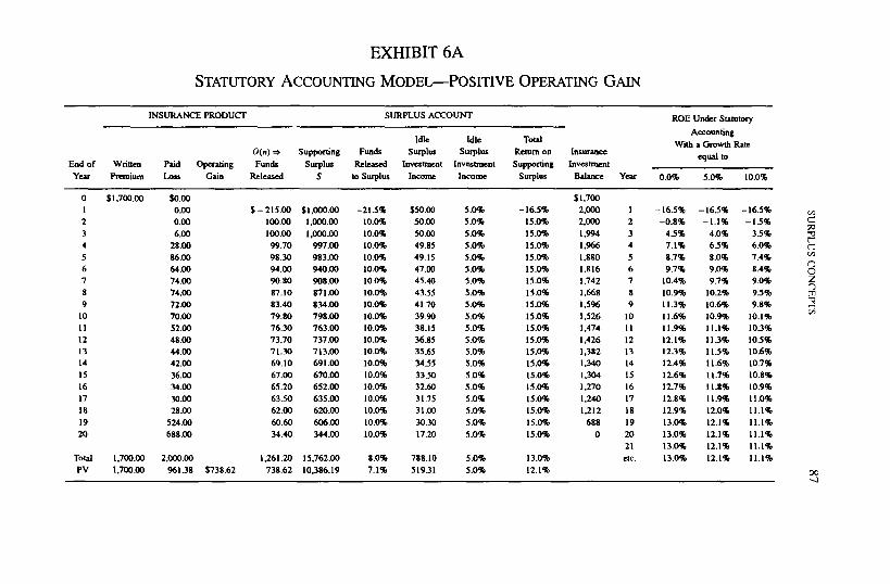
EXHIBIT 6A

STATUTORY ACCOUNTING MODEL--POSITIVE OPERATING GAIN

INSURANCE PRODUCT SURPLUS ACCOUNT ROE Under Statutory

Aoeoun6n 8 Idle idle Total With a Cnowth Rate

O(n) =~ Supporting Funds Sm'plus Surplus Return on Insurance equal to End of Written Paid Operating Funds Su~lus Released Investment Investment Supporting Investment Year P'nmfium Loss Gain Released S to Surplus Income Income Surplus Balance Year 0.0% 5.0% 10.0%

0 $13 00.00 $0 .o0 I 0.o0

2 0.o0

3 6.00

4 28.00

5 86.o0

6 64.00

7 74.00 8 74,O0 9 72.00

I 0 70.00 I I 52.00

12 48.0O 13 44.00

14 42.00 15 36.00 16 34.O0 17 30.00 18 28.O0 19 524.00 20 688.00

Total 1300.00 2,000.00 PV 1 ,700_00 961.38 $738.62

$ - 215.00 $1,000.00 -21.5% $50.00 5.0% -16.5% 100.00 1,O00.O0 10.0% 50.00 5.0~ 15.0% 100.00 1,000.00 10.0% 50.00 5.0% 15.0% 99.70 997.00 10.0% 49.85 5.0% 15.0% 98.30 983.00 10.0% 49.15 5.0% 15.0% 94.00 940.00 10.0% 47.00 5.0% 15.0% 90.80 908.00 10.0% 45.40 5.0% 15.0% 87.10 871.00 10.0% 43.55 5.0% 15.0% 83.40 834.00 10.0% 4130 5.0% 15.0% 79.80 798.00 10.0% 39.90 5.0% 15.0% 76.30 763.00 10.0% 38.15 5.0% 15.0% 73.70 737.00 10.0% 36.85 5.0% 15.0% 71.30 713.00 10.0% 35.65 5.0% 15.0% 69.10 691.00 10.0% 34.55 5.0% 15.0% 67.00 670.00 10.0% 33.50 5.0% 15.0% 65.20 652.00 10.0% 32.60 5.0% 15.0%

63.50 635.00 10.0% 31.75 5.0% 15.0%

62.00 620.00 10.0% 31.00 5.0% 15.0%

60.60 606 .O0 I 0.0% 30.30 5.0% 15.0%

34.40 344.00 10.0% 17.20 5.0% 15.0%

1,261.20 15,762.00 8.0% 788.10 5.0% 13.0% 738.62 10,386.19 7.1% 519.31 5.0% 12.1%

$1,700 2,000 I -16.5% -16.5% -16.5% 2,000 2 -0.8% -1.1% -I .5% 1,994 3 4.5% 4.0% 3.5% 1,966 4 7.1% 6.5% 6.0% 1,880 5 8.7% 8.0% 7.4% 1,816 6 9.7% 9.0% 8.4% 1,742 7 10.4% 9.7% 9.0% 1,668 8 10.9% 10.2% 9.5% 1,596 9 11.3% 10.6% 9.8% 1,526 10 11.6% 1 0 . 9 % 10.1% 1,474 11 I 1 .9% 1 1 . 1 % 10.3% 1,426 12 12.1% il.3% 10.5% 1,382 13 12.3% 1 1 - 5 % 10.6% 1,340 14 12.4% 11.6% 10.7%

1,304 15 12.6% II.7% 10.8%

1,270 16 12.7% I 1.8% 10.9%

1,240 17 12.8% 11.9% 11.0%

1,212 18 12.9% 1 2 - 0 % 11.1% 688 19 13.0% 1 2 . 1 % I1.1%

0 20 13.0% 1 2 . 1 % 11.1% 21 13.0% 1 2 . 1 % I1.|% etc. 13.0% 1 2 . 1 % 11.1%

O¢ "-d

88 SURPLUS CONCEPTS

EXHIBIT 6B

POS ITIVE OPERATING G A I N FROM THE I N S U R A N C E C A R R I E R



End of Invested Invested Paid Required Invested Released Flows Year Surplus Premium Loss Funds Funds to Surplus for IRR

0 $261.38 $1,700.00 $0.00 $1,961.38 $1,961.38 $0.00 $-261 .38 1 0.00 2,009.45 2,059.45 50.00 50.00 2 0.00 2,059.92 2,109.92 50.00 50.00 3 6.00 2,103.92 2,156.92 53.00 53.00 4 28.00 2,117.26 2,181.12 63.86 63.86 5 86.00 2,044.98 2,137.12 92.14 92.14 6 64.00 2,004.23 2,083.23 79.00 79.00 7 74.00 1,948.04 2,030.44 82.40 82.40 8 74.00 1,890.89 1,971.44 80.55 80.55 9 72.00 1,835.73 1,913.43 77.70 77.70

10 70.00 1,782.62 1,857.52 74.90 74.90 11 52.00 1,755.60 1,819.75 64.15 64.15 12 48.00 1,734.53 1,795.38 60.85 60.85 13 44.00 1,719.61 1,777.26 57.65 57.65 14 42.00 1,708.04 1,763.59 55.55 55.55 15 36.00 1,705.94 1,757.44 51.50 51.50 16 34.00 1.707.64 1,757.24 49.60 49.60 17 30.00 1,716.27 1,763.02 46.75 46.75 18 28.00 1,729.08 1,774.08 45.00 45.00 19 524.00 999.24 1,291.53 292.29 292.29 20 688.00 0.00 361.20 361.20 361.20

IRR = 24.4%

EXHIBIT 7

THE MODIFIED BINGHAM MODEL


Idle Idle Total O(n) ~ Supporting Funds Surplus Surplus Return on Total


0 $400.00 $0.00 1 264.00 $12.08 $187.93 6.43% $9.40 5.0% 11.43% 2 96.00 7.14 110.97 6.43% 5.55 5.0% 11.43% 3 32.00 4.01 62.40 6.43% 3.12 5.0% 11.43% 4 8.00 2.10 32.63 6.43% 1.63 5.0% 11.43% 5 4.00 1.23 19.14 6.43% 0.96 5.0% 11.43%

NPV 400.00 375.86 $24.14 24.14 375.38 6.43% 18.77 5.0% 11.43% Average = 11.43%

$ - 187.93 $ -4 .00 $400.00 $24.14 98.44 3.92 143.92 13.26 61.25 3.98 47.98 6.79 36.90 2.36 14.36 3.11 17.22 0.98 4.98 1.17 21.33 0.00 0.00 0.00

IRR = 11.43%

Determination of the {O(n)}

1. Constant annual ROE ~ O(n)/S(n) = k, or O(n) = k *S(n)

2. NPV({O(n)}) = k *NPV({S(n)}) =~ k = NPV({O(n)})/NPV({S(n)})

n S(n) O(n) 1 S(I) = $187.93 $12.08 2 S(2)= 110.97 7.14 3 S(3)= 62.40 4.01 4 S(4)= 32.63 2.10 5 S(5)= 19.14 123

NPV({S(n)}) = $375.38 NPV({O(n)}) = $ 24.14 $24.14

k = 0.064303 ",,D

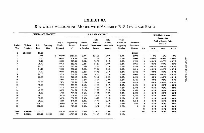
EXHIBIT 8A

STATUTORY ACCOUNTING MODEL WITH VARIABLE R" S LEVERAGE RATIO

".,D O

I N S U R A N C E PRODUCT S U R P L U S A C C O U N T ROE Under Statutory

Account ing Idle Idle Total

With a Growth Rate 0 ( - ) =~ Support ing Funds Surplus Surplus Return on Insurance equal to

End of W r i , e n Paid Operating Funds Surplus Released Investment Investment Support ing Investment

Year Premium Loss Gain Released S to Surp lus Income Income Surplus Balance Year 0 .0% 5.0% 10.0%

0 $1,000.00 $0.00

1 0 .00 $ - 950 00 $480.69 - 2 . 0 % $24.03 0 0 % - 1.9% 2 0 .00 100.00 504.73 0 .2% 2 5 1 4 0.1% 0 1 %

3 6.00 100.00 529.96 0 .2% 26.50 0.1% 0.2% 4 28.00 99.70 553.46 0 .2% 27.67 0.0% 0.2%

5 86.00 98.30 567.13 0.2% 28.36 O. 1% 0.2%

6 64.00 94.00 552.49 0.2% 27.62 0~3% 0.2%

7 74.00 90.80 548.12 0 .2% 27.41 0.1% 0.2% 8 74.00 87.10 5 3 8 5 2 0 .2% 26.93 0.1% 0.2% 9 72.00 83A0 528A5 0 .2% 26.42 0.0% 0.2%

10 70.00 79.80 518.87 0 .2% 25.94 0.0% 0.2% 11 52.00 76.30 509.81 0 .1% 25.49 0.0% 0.2% 12 48 .00 73.70 509.30 0 .1% 25.47 0.1% 0 1 % 13 44.00 71.30 510.77 0 .1% 25 54 0.1% 0.2% 14 42.00 69.10 514.31 0 .1% 25.72 0.1% 0.2% 15 36.00 67.00 519.02 0 .1% 25.95 0.0% 0.2% 16 34.00 65.20 5 2 6 9 7 0 .1% 26.35 0.1% 0.2%

17 30.00 63 50 536.32 0 .1% 26.82 0.1% 0.2% 18 28.00 62.00 548.14 0 .1% 27.41 0.1% 0.2% 19 524.00 6060 561.54 0.1% 28.08 0.1% 0 1 % 20 688.00 34.40 327.62 0.1% 16.38 0.0% 0.2%

Total 1,000.00 2,000.00 PV 1,000.00 961.38 $38.62

526.20 10,386.22 0 .1% 519.31 38.62 6,509 42 0 .1% 325.47

0.0% 0.1% 0.0% 0.1%

$1,000

2,000 1 - 1 . 9 % - 1 . 9 % - 1 . 9 %

2,000 2 - 0 8 % - 0 . 8 % - 0 . 9 % I , ~ 4 3 -0 .4% -0 .5% --0.5% 1.966 4 - 0 3 % - 0 . 3 % - 0 3 %

1,880 5 -0 .2% - 0 . 2 % -0 .2% 1,816 6 -0 .1% - 0 . 1 % -0 .2% 1.742 7 - 0 . 0 % --0.1% - 0 . 1 % 1,668 8 -0 .0% - 0 . 1 % - 0 .1% 1.596 9 0 .0% - 0 . 0 % - 0 . 1 %

1.526 10 0.0% - 0 . 0 % - 0 . 1 % 1,474 11 0.0% - 0 . 0 % - 0 . 1 %

1,426 12 0 A % 0.0% - 0 . 0 % 1,382 13 0.1% 0.0% - 0 . 0 % 1,340 14 0.1% 0.0% -0.0% 1,304 15 0.1% 0.0% - 0 0 % 1,270 16 0.1% 0.0% - 0 . 0 % 1,240 17 0.1% 0.0% - 0 . 0 % 1,212 18 0.1% 0.1% - 0 . 0 %

688 19 0.1% 0.1% 0.0% 0 20 O 1 % 0.1% 0.0%

21 0.1% 0.1% 0.0% elc. 0 .1% 0.1% 0.0%

0 Z

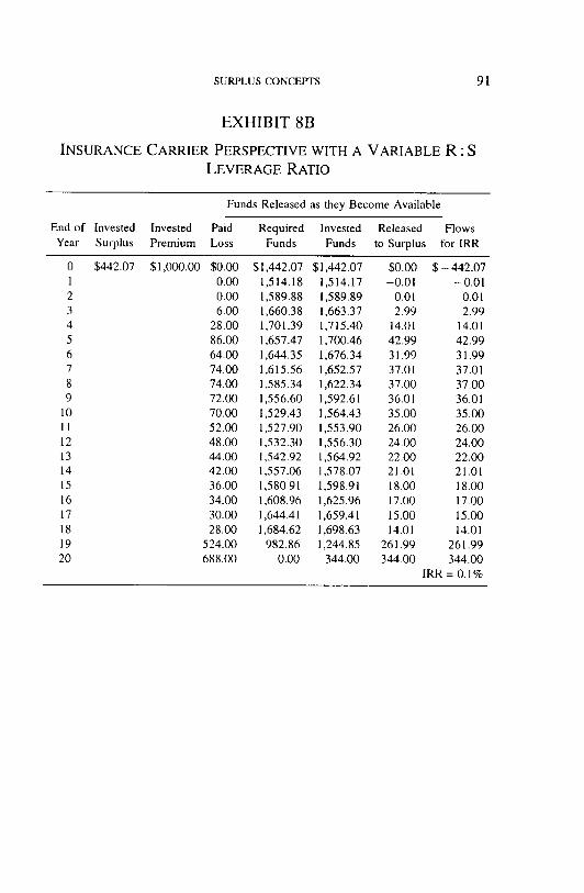
SURPLUS CONCEPTS 91

EXHIBIT 8B

I N S U R A N C E C A R R I E R P E R S P E C T I V E WITH A V A R I A B L E R : S

L E V E R A G E RATIO


End of Invested Invested Paid Required Invested Released Flows Year Surplus Premium Loss Funds Funds to Surplus for IRR

0 $442.07 $1,000.00 $0.00 $1,442.07 $1,442.07 $0.00 $-442 .07 1 0.00 1,514.18 1,514.17 -0.01 -0.01 2 0.00 1,589.88 1,589.89 0.01 0.01 3 6.00 1,660.38 1,663.37 2.99 2.99 4 28.00 1,701.39 1,715.40 14.01 14.01 5 86.00 1,657.47 1,700.46 42.99 42.99 6 64.00 1,644.35 1,676.34 31.99 31.99 7 74.00 1,615.56 1,652.57 37.01 37.01 8 7&00 1,585.34 1,622.34 37.00 37.00 9 72.00 1,556.60 1,592.61 36.01 36.01

10 70.00 1,529.43 1,564.43 35.00 35.00 I 1 52.00 1,527.90 1,553.90 26.00 26.00 12 48.00 1,532.30 1,556.30 24.00 24.00 13 44.00 1,542.92 1,564.92 22.00 22.00 14 42.00 1,557.06 1,578.07 21.01 21.01 15 36.00 1,580.91 1,598.91 18.00 18.00 16 34.00 1,608.96 1,625.96 17.00 17.00 17 30.00 1,644.41 1,659.41 15 ~00 15.00 18 28.00 1,684.62 1,698.63 14.01 14.01 19 524.00 982.86 1,244.85 261.99 261.99 20 688.00 0.00 344.00 344.00 344.00

IRR = 0.1%

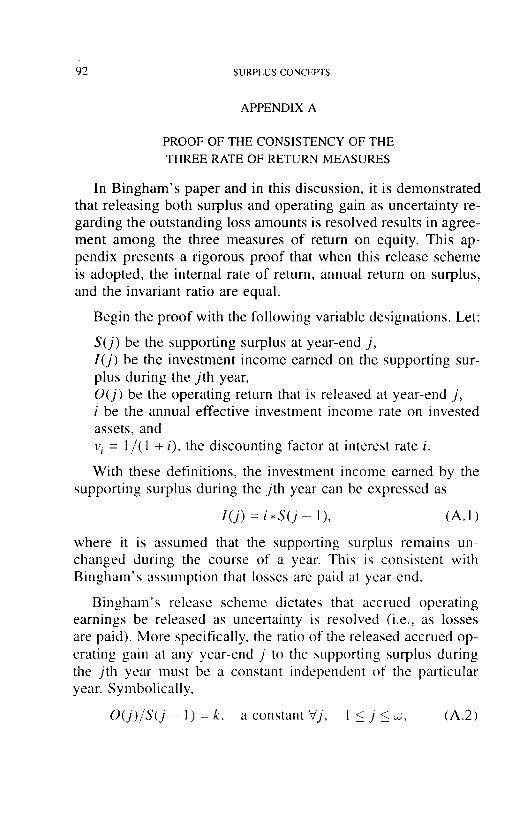
92 SURPLUS CONCEFFS

APPENDIX A

PROOF OF THE CONSISTENCY OF THE THREE RATE OF RETURN MEASURES

In Bingham's paper and in this discussion, it is demonstrated that releasing both surplus and operating gain as uncertainty regarding the outstanding loss amounts is resolved results in agreement among the three measures of return on equity. This appendix presents a rigorous proof that when this release scheme is adopted, the internal rate of return, annual return on surplus, and the invariant ratio are equal.

Begin the proof with the following variable designations. Let:

S(j) be the supporting surplus at year-end j, I ( j ) be the investment income earned on the supporting surplus during the j th year, O(j) be the operating return that is released at year-end j, i be the annual effective investment income rate on invested assets, and v i = 1/(1 + i), the discounting /actor at interest rate i.

With these definitions, the investment income earned by the supporting surplus during the j th year can be expressed as

l ( j ) = i . S ( j - 1), (A.1)

where it is assumed that the supporting surplus remains unchanged during the course of a year. This is consistent with Bingham's assumption that losses are paid at year-end.

Bingham's release scheme dictates that accrued operating earnings be released as uncertainty is resolved (i.e., as losses are paid). More specifically, the ratio of the released accrued operating gain at any year-end j to the supporting surplus during the j th year must be a constant independent of the particular year. Symbolically,

O ( j ) / S ( j - 1) = k, a constant V j, 1 _< j <_ ~,, (A.2)

SURPLUS CONCEPTS 93

where 9, denotes the end of the last year during which there are open (or IBNR) claims. Note that a second requirement placed upon the set of released operating gains is that the present value of the {O(j)} equals the present value of the operating gain. While this requirement insures releasing an amount exactly equal to the accrued operating gain, it is not a necessary condition for agreement of the three measures of ROE.

Upon soh'ing Equation A.2 for O(j) , we obtain the released operating earnings at the end of the jth year in terms of the supporting surplus that was allocated at the end of the previous year,

O(j) = k , S ( j - 1). (A.3)

During the j th year, the supporting surplus is S ( j - 1) and the return on that surplus is the investment income on that surplus, l ( j ) , plus the released operating gain, O(j) , or

l ( j ) + O( j ) = (i + k ) , S ( j - 1). (A.4)

Dividing by the invested surplus, S( j - 1), gives the average re- ttttvt on surplus during the j th 3'ear, (i + k). This expression is independent of j , making it a constant for all years.

Taking the present value of the total return on supporting surplus using any interest rate gives

N P V [ I ( j ) + O ( j ) ] = ( i + k ) , N P V [ S ( j - 1)]. (A.5)

Divide the present value of the total return by the present value of the year-end supporting surplus, to obtain Bingham's present value ratio,

NPV[I( j) + O ( j ) ] / N P V [ S ( j - l)l = (i + k). (A.6)

Note that the present value ratio is equal to the average return on surplus.

To show that the IRR of the surplus flows is also equal to the present value ratio and average return on surplus, begin by

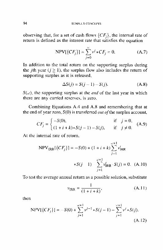
94 SURPLUS CONCEPTS

observing that, for a set of cash flows {C~}, the internal rate of return is defined as the interest rate that satisfies the equation

NPV[{CFj}] = ~ v j .CFj = 0. (A.7) j=0

In addition to the total return on the supporting surplus during the j th year (j _> 1), the surplus flow also includes the return of supporting surplus as it is released,

A S ( j ) = S ( j - 1 ) - S ( j ) . (A.8)

S(~), the supporting surplus at the e n d of the last year in which there are any carried reserves, is zero.

Combining Equations A.4 and A.8 and remembering that at the end of year zero, S(0) is transferred out of the surplus account,

- S ( 0 ) , i f j = 0, (A.9) CFj= (l+i+k),S(j-1)-S(j), i f j ¢ 0 .

At the internal rate o f return,

a. ,+ 1

NPVIRR[{CFj}I = - S ( 0 ) + (1 + i + k) ~ V~R R j = l

,~'+ 1

*S(j-1)-~vlR R . S ( j ) = 0 . ( a . 1 0 ) j = l

To test the average annual return as a possible solution, substitute

1 VIR R - - . . , (A. 1 1 ) ( 1 i + + K)

then

~,+ 1 ~ , + 1

NPV[{C~}] = -S(0) + ~ v j -1 , S ( j - 1 ) - ~ v j , S ( j ) . j = l j = l

(A. 12)

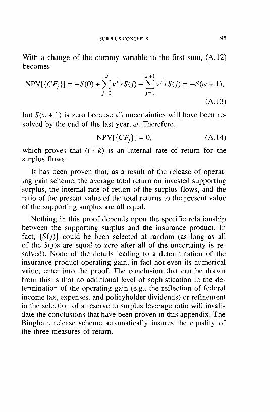
SURPLUS CONCEPTS 95

With a change of the dummy variable in the first sum, (A.12) becomes

a~ w,+l

NPV[{CFj}] = -S(0) + ~ v j , S ( j ) - ~ v j , S ( j ) = - S ( w + 1), j = 0 j = l

(A.13)

but S(o~ + l) is zero because all uncertainties will have been resolved by the end of the last year, ~. Therefore,

NPV[{CFj}] = 0, (A.14)

which proves that (i + k) is an internal rate of return for the surplus flows.

It has been proven that, as a result of the release of operating gain scheme, the average total return on invested supporting surplus, the internal rate of return of the surplus flows, and the ratio of the present value of the total returns to the present value of the supporting surplus are all equal.

Nothing in this proof depends upon the specific relationship between the supporting surplus and the insurance product. In fact, {S(j)} could be been selected at random (as long as all of the S(j)s are equal to zero after all of the uncertainty is resolved). None of the details leading to a determination of the insurance product operating gain, in fact not even its numerical value, enter into the proof. The conclusion that can be drawn from this is that no additional level of sophistication in the determination of the operating gain (e.g., the reflection of federal income tax, expenses, and policyholder dividends) or refinement in the selection of a reserve to surplus leverage ratio will invali- date the conclusions that have been proven in this appendix. The Bingham release scheme automatically insures the equality of the three measures of return.

96 SURPLUS CONCEIY['S

A P P E N D I X B

EVIDENCE FOR A DECREASING LEVERAGE RATIO

Workers compensation is often cited as a line of business in which the uncertainty in the outstanding loss reserve decreases rapidly because of the highly predictable nature of lifetime pension cases. The conventional wisdom is that once the more volatile minor cases have been resolved, all that remains are claimants with lifetime benefits. As soon as the open claims consist only of lifetime pension cases, supporting surplus can be released rapidly. In particular, as a result of a decision of the hearing officer during the workers compensation rating hearing for rates to become effective January 1, 1988 in Massachusetts, the leverage ratio increases uniformly from the end of the fifth quarter until all claims are closed [3]. The pension case argument has been used to support the accelerated release of surplus.

Workers compensation claims probably arise from several underlying distributions. Clearly, minor cuts and bruises cannot be described by the same severity distribution that would apply to more serious injuries of the type that can lead to long term dis- ability. As groups of claims close, the remaining open claims may be of a more homogeneous nature. This, in itself, may decrease the relative uncertainty in the open claim reserves. Ini- tially, at least, as certain classes of claims close, an increase in the leverage ratio may be possible.

Once the population of open claims consists of nothing but lifetime pension cases, the long term behavior of the leverage ratio manifests itself. For a reasonable example, it can be demonstrated that the leverage ratio must decrease over time. This is not a rigorous proof that the leverage ratio for workers compensation coverage must always decrease but, rather, it is evidence that one cannot assume that once pension cases dominate the open claim reserves, the leverage ratio will always increase. This appendix serves as a counter example, disproving the common contention.

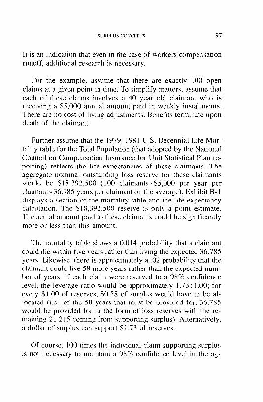
SURPLUS CONC~:~PTS 97

It is an indication that even in the case of workers compensation runoff, additional research is necessary.

For the example, assume that there are exactly 100 open claims at a given point in time. To simplify matters, assume that each of these claims involves a 40 year old claimant who is receiving a $5,000 annual amount paid in weekly installments. There are no cost of living adjustments. Benefits terminate upon death of the claimant.

Further assume that the 1979-1981 U.S. Decennial Life Mor- tality table for the Total Population (that adopted by the National Council on Compensation Insurance for Unit Statistical Plan re- porting) reflects the life expectancies of these claimants. The aggregate nominal outstanding loss reserve for these claimants would be $18,392,500 (100 c la imants .S5,000 per year per c la imant . 36.785 years per claimant on the average). Exhibit B- 1 displays a section of the mortality table and the life expectancy calculation. The $18,392,500 reserve is only a point estimate. The actual amount paid to these claimants could be significantly more or less than this amount.

The mortality table shows a 0.014 probability that a claimant could die within five years rather than living the expected 36.785 years. Likewise, there is approximately a .02 probability that the claimant could live 58 more years rather than the expected number of years. If each claim were reserved to a 98% confidence level, the leverage ratio would be approximately 1.73 : 1.00; for every $1.00 of reserves, $0.58 of surplus would have to be allocated (i.e., of the 58 years that must be provided for, 36.785 would be provided for in the form of loss reserves with the remaining 21.215 coming from supporting surplus). Alternatively, a dollar of surplus can support $1.73 of reserves.

Of course, 100 times the individual claim supporting surplus is not necessary to maintain a 98% confidence level in the ag-

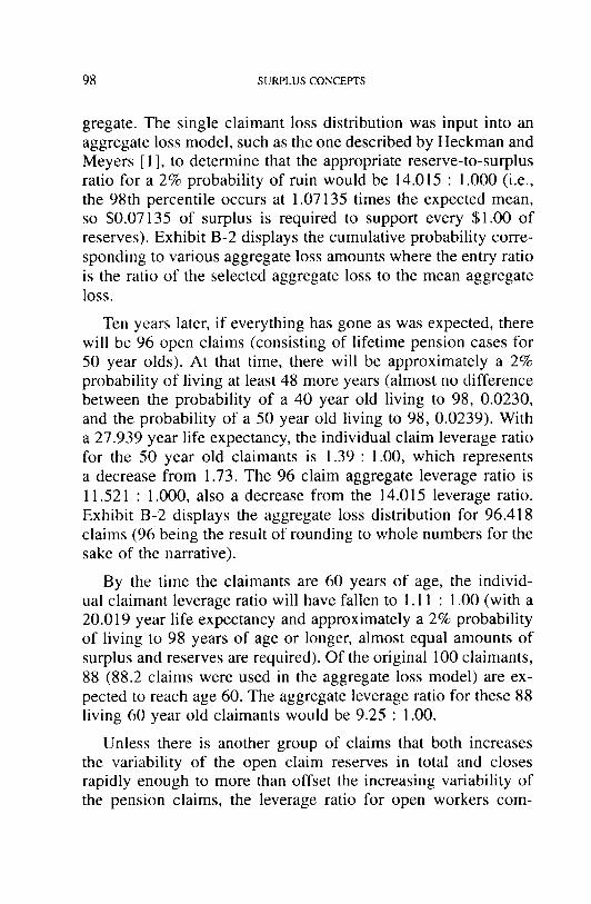
98 SURPLUS CONCEPTS

gregate. The single claimant loss distribution was input into an aggregate loss model, such as the one described by Heckman and Meyers [1], to determine that the appropriate reserve-to-surplus ratio for a 2% probability of ruin would be 14.015 : 1.000 (i.e., the 98th percentile occurs at 1.07135 times the expected mean, so $0.07135 of surplus is required to support every $1.00 of reserves). Exhibit B-2 displays the cumulative probability corresponding to various aggregate loss amounts where the entry ratio is the ratio of the selected aggregate loss to the mean aggregate loss.

Ten years later, if everything has gone as was expected, there will be 96 open claims (consisting of lifetime pension cases for 50 year olds). At that time, there will be approximately a 2% probability of living at least 48 more years (almost no difference between the probability of a 40 year old living to 98, 0.0230, and the probability of a 50 year old living to 98, 0.0239). With a 27.939 year life expectancy, the individual claim leverage ratio for the 50 year old claimants is 1.39 : 1.00, which represents a decrease from 1.73. The 96 claim aggregate leverage ratio is 11.521 : 1.000, also a decrease from the 14.015 leverage ratio. Exhibit B-2 displays the aggregate loss distribution for 96.418 claims (96 being the result of rounding to whole numbers for the sake of the narrative).

By the time the claimants are 60 years of age, the individual claimant leverage ratio will have fallen to 1.11 : 1.00 (with a 20.019 year life expectancy and approximately a 2% probability of living to 98 years of age or longer, almost equal amounts of surplus and reserves are required). Of the original 100 claimants, 88 (88.2 claims were used in the aggregate loss model) are expected to reach age 60. The aggregate leverage ratio for these 88 living 60 year old claimants would be 9.25 : 1.00.

Unless there is another group of claims that both increases the variability of the open claim reserves in total and closes rapidly enough to more than offset the increasing variability of the pension claims, the leverage ratio for open workers corn-

SURPLUS CONCEPTS 99

pensation claims must decrease in the long run. The preceding example does not constitute a proof that the leverage ratio decreases; rather, it makes the conventional wisdom less obvious. The appropriate leverage ratio for any line of business must be the result of an investigation of the underlying volatility of its open claims at any point in time.

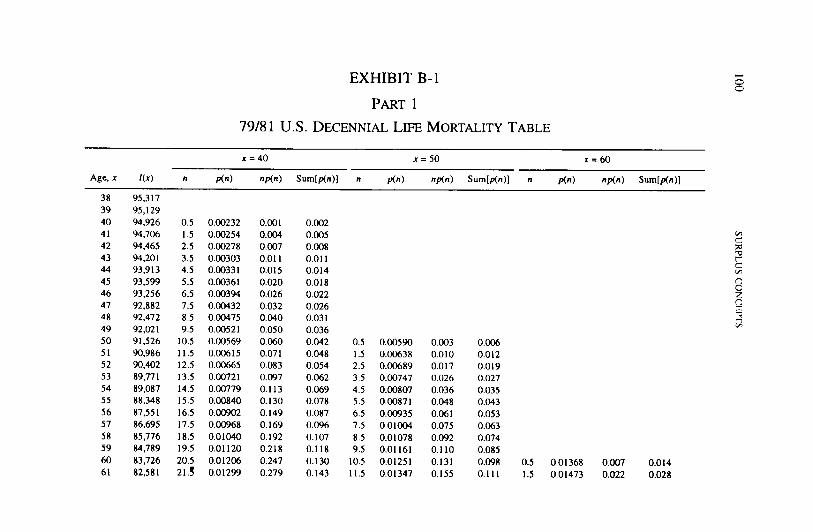
EXHIBIT B-1

PART 1

79•81 U.S. DECENNIAL LIFE MORTALITY TABLE

m

O C,

x = 40 x = 50 x = 60

Age, x l(x) n p(n) np(n) Sum[p(n)] n IXn) np(n) Sum[p(n)] n p(n) np(n) Sum[p(n)]

38 95,317 39 95,129 40 94,926 0.5 0.00232 0.001 0.002 41 94,706 1.5 0.00254 0.004 0.005 42 94,465 2.5 0.00278 0.007 0.008 43 94,201 3.5 0.00303 0.011 0.011 44 93,913 4.5 0.00331 0.015 0.014 45 93,599 5.5 0.00361 0.020 0.018 46 93,256 6.5 0.00394 0.026 0.022 47 92,882 7.5 0.00432 0.032 0.026 48 92,472 8.5 0.00475 0.040 0.031 49 92,021 9.5 0.00521 0.050 0.036 50 91,526 10.5 0.00569 0.060 0.042 0.5 0.00590 0.003 0.006 51 90,986 11.5 0.00615 0.071 0.048 1.5 0.00638 0.010 0.012 52 90,402 12.5 0.00665 0.083 0.054 2.5 0.00689 0.017 0.019 53 89,771 13.5 0.00721 0.097 0.062 3.5 0.00747 0.026 0.027 54 89,087 14.5 0.00779 0.113 0.069 4.5 0.00807 0.036 0.035 55 88,348 15.5 0.00840 0.130 0.078 5.5 0.00871 0.048 0.043 56 87,551 16.5 0.00902 0.149 0.087 6.5 0.00935 0.061 0.053 57 86,695 17.5 0.00968 0.169 0.096 7.5 0.01004 0.075 0.063 58 85,776 18.5 0.01040 0.192 0.107 8.5 0.01078 0.092 0.074 59 84,789 19.5 0.01120 0.218 0.118 9.5 0.01161 0.110 0.085 60 83,726 20.5 0.01206 0.247 0.130 10.5 0.01251 0.131 0.098 0.5 0.01368 0.007 0.014 61 82,581 21.~ 0.01299 0.279 0.143 11.5 0.01347 0.155 0.111 1.5 0.01473 0.022 0.028

t-- f~

© Z

EXHIBIT B-1

PART 2


X = 4 0 x = 5 0 x = 6 0

Age, x t(x) n p(n) rip(n) Sum[p(n)] n p(n) np(n) Sum[p(n)] n p(n) np(n) Sum[p(n)]

62 81,348 22.5 0.01395 0.314 0.157 12.5 0.01447 0.181 0.126 2.5 0.01581 0.040 0.044 63 80,024 23.5 0.01491 0.350 0.172 13.5 0.01546 0.209 0.141 3.5 0.01690 0.059 0.061 64 78,609 24.5 0.01582 0.388 0.188 14.5 0.01641 0.238 0.158 4.5 0.01794 0.081 0.079 65 77,107 25.5 0.01672 0.426 0.204 15.5 0.01734 0.269 O. 175 5.5 0.01895 O. 104 0.098 66 75,520 26.5 0.01763 0.467 0.222 16.5 0.01829 0.302 0.193 6.5 0.01999 0.130 0.118 67 73,846 27.5 0.01858 0.511 0.241 17.5 0.01927 0.337 0.212 7.5 0.02107 0.158 0.139 68 72,082 28.5 0.01964 0.560 0.260 18.5 0.02037 0.377 0.233 8.5 0.02226 0.189 0.161 69 70,218 29.5 0.02075 0.612 0.281 19.5 0.02152 0.420 0.254 9.5 0.02353 0.224 0.185 70 68,248 30.5 0.02194 0.669 0.303 20.5 0.02276 0.467 0.277 10.5 0.02488 0.261 0.210 71 66,165 31.5 0.02310 0.728 0.326 21.5 0.02396 0.515 0.301 II.5 0.02619 0.301 0.236 72 63,972 32.5 0.02422 0.787 0.350 22.5 0.02512 0.565 0.326 12.5 0.02746 0.343 0.263 73 61,673 33.5 0.02522 0.845 0.376 23.5 0.02616 0.615 0.352 13.5 0.02859 0.386 0.292 74 59,279 34.5 0.02613 0.901 0.402 24.5 0.02710 0.664 0.379 14.5 0.02962 0.429 0.322 75 56,799 35.5 0.02697 0.957 0.429 25.5 0.02797 0.713 0.407 15.5 0.03058 0.474 0.352 76 54,239 36.5 0.02781 i .015 0.456 26.5 0.02884 0.764 0.436 16.5 0.03153 0.520 0.384 77 51,599 37.5 0.02866 1.075 0.485 27.5 0.02973 0.818 0.466 17.5 0.03250 0.569 0.416 78 48,878 38.5 0.02957 1.138 0.515 28.5 0.03067 0.874 0.497 18.5 0.03353 0.620 0.450 79 46,071 39.5 0.03046 1.203 0.545 29.5 0.03159 0.932 0.528 19.5 0.03453 0.673 0.484 80 43,180 40.5 0.03131 1.268 0.576 30.5 0.03247 0.990 0.561 20.5 0.03550 0.728 0.520 81 40,208 41.5 0.03198 1.327 0.608 31.5 0.03317 1.045 0.594 21.5 0.03626 0.780 0.556 82 37,172 42.5 0.03241 1.378 0.641 32.5 0.03362 1.093 0.627 22.5 0.03675 0.827 0.593 83 34,095 43.5 0.03248 1.413 0.673 33.5 0.03368 1.128 0.661 23.5 0.03682 0.865 0.630 84 31,012 44.$ 0.03215 1.431 0.705 34.5 0.03335 1.150 0.695 24.5 0.03645 0.893 0.666 85 27,960 45.5 0.03159 1.437 0.737 35.5 0.03277 1.163 0.727 25.5 0.03582 0.913 0.702 86 24,961 46.5 0.03079 1.432 0.768 36.5 0.03194 1.166 0.759 26.5 0.03491 0.925 0.737 87 22,038 47.5 0.02953 1.403 0.797 37.5 0.03063 1.148 0.790 27.5 0.03348 0.921 0.770 88 19,235 48.5 0.02778 1.347 0.825 38.5 0.02881 1.109 0.819 28.5 0.03150 0.898 0.802 89 16,598 49.5 0.02575 1.274 0.851 39.5 0.02670 1.055 0.845 29.5 0.02919 0.861 0.831

t'-

o z PJ

EXHIBIT B- 1

PART 3


x = 4 0 x = 50 x = 6 0

Age, x I(x) n p(n) np(n) Sum[p(n)] n p(n) rip(n) Sum[p(n)] n p(n) np(n) Sum[p(n)]

90 14,154 50.5 0.02366 1.195 0.875 40.5 0.02454 0.994 0.870 30.5 0.02683 0.818 0.858 91 11,908 51.5 0.02154 1.109 0.896 41.5 0.02234 0.927 0.892 31.5 0.02442 0.769 0.882 92 9,863 52.5 0.01929 1.013 0.915 42.5 0.02001 0.850 0.912 32.5 0.02187 0.711 0.904 93 8,032 53.5 0.01694 0.906 0.932 43.5 0.01757 0.764 0.930 33.5 0.01921 0.643 0.923 94 6,424 54.5 0.01455 0.793 0.947 44.5 0.01509 0.671 0.945 34.5 0.01649 0.569 0.940 95 5,043 55.5 0.01221 0.678 0.959 45.5 0.01266 0.576 0.958 35.5 0.01384 0.491 0.954 96 3,884 56.5 0.00996 0.562 0.969 46.5 0.01032 0.480 0.968 36.5 0.01129 0.412 0.965 97 98 99

100 101 102 103 104 105 106 107 108 109 110

2,939 57.5 0.00794 0.457 0.977 47.5 0.00824 0.391 0.976 37.5 0.00901 0.338 0.974 2,185 58.5 0.00618 0.362 0.983 48.5 0.00641 0.311 0.983 38.5 0.00701 0.270 0.981 1,598 59.5 0.00472 0.281 0.988 49.5 0.00489 0.242 0.987 39.5 0.00535 0.211 0.986 i ,150 60.5 0.00353 0.214 0.991 50.5 0.00366 0.185 0.991 40.5 0.00400 0.162 0.990

815 61.5 0.00258 0.159 0.994 51.5 0.00268 0.138 0.994 41.5 0.00293 0.121 0_993 570 62.5 0.00186 0AI7 0.996 52.5 0.00193 0.102 0.996 42.5 0.00211 0.090 0.995 393 63.5 0.00133 0.084 0.997 53.5 0.00138 0.074 0.997 43.5 0.00150 0.065 0.997 267 64.5 0.00093 0.060 0.998 54.5 0.00096 0.052 0.998 44.5 0.00105 0.047 0.998 179 65.5 0.00063 0.041 0.999 55.5 0.00066 0.036 0.999 45.5 0.00072 0.033 0.999 119 66.5 0.00043 0.029 0.999 56.5 0.00045 0.025 0.999 46.5 0.00049 0.023 0.999 78 67.5 0.00028 0.019 0.999 57.5 0.00029 0.017 0.999 47.5 0.00032 0.015 0.999 51 68.5 0.00019 0.013 1.000 58.5 0.00020 0.012 1.000 48.5 0.00021 0.010 1.000 33 69.5 0.00035 0.024 1.000 59.5 0.00036 0.021 1.000 49.5 0.00039 0.020 1.000

0 70.5 0.0(X)00 0.000 1.000 60.5 0.00000 0.000 1.000 50.5 0.00000 0.000 1.000 Total 1.000013 36.785 1.001X~ 27.939 1.00000 20.019

w

0 Z

ETI

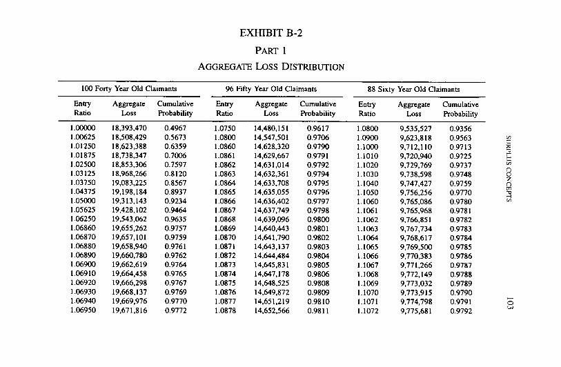
EXHIBIT B-2

PART I

AGGREGATE LOSS DISTRIBUTION

100 Forty Year Old Claimants

Entry Aggregate Cumulative Ratio Loss Probability

96 Fifty Year Old Claimants


88 Sixty Year Old Claimants


1.0(K)~ 18,393,470 0.4967 1.00625 18,508,429 0.5673 1.01250 18,623,388 0.6359 1.01875 18,738,347 0.7006 1.02500 18,853,306 0.7597 1.03125 18,968,266 0.8120 1.03750 19,083,225 0.8567 1.04375 19,198,184 0.8937 1.05000 19,313,143 0.9234 1.05625 19,428,102 0.9464 1.06250 19,543,062 0.9635 1.06860 19,655,262 0.9757 1.06870 19,657,101 0.9759 1.06880 19,658,940 0.9761 1.06890 19,660,780 0.9762 1.06900 19,662,619 0.9764 1.06910 19,664,458 0.9765 1.06920 19,666,298 0.9767 1.06930 19,668,137 0.9769 1.06940 19,669,976 0.9770 1.06950 19,671,816 0.9772

1.0750 14,480,151 0.9617 1.0800 14,547,501 0.9706 1.0860 14,628,320 0.9790 1.0861 14,629,667 0.9791 1.0862 14,631,014 0.9792 1.0863 14,632,361 0.9794 1.0864 14,633,708 0.9795 1.0865 14,635,055 0.9796 1.0866 14,636,402 0.9797 1.0867 14,637,749 0.9798 1.0868 14,639,096 0.9800 1.0869 14,640,443 0.9801 1.0870 14,641,790 0.9802 1.0871 14,643,137 0.9803 1.0872 14,644,484 0.9804 1.0873 14,645,831 0.9805 1.0874 14,647,178 0.9806 1.0875 14,648,525 0.9808 1.0876 14,649,872 0.9809 1.0877 14,651,219 0.9810 1.0878 14,652,566 0.9811

1.0800 9,535,527 0.9356 1.0900 9,623,818 0.9563 I.I000 9,712,1 I0 0.9713 1.1010 9,720,940 0.9725 1.1020 9,729,769 0.9737 I.I030 9,738,598 0.9748 1.1040 9,747,427 0.9759 I.I050 9,756,256 0.9770 1.1060 9,765,086 0.9780 1.1061 9,765,968 0.9781 1.1062 9,766,851 0.9782 1.1063 9,767,734 0.9783 1.1064 9,768,617 0.9784 1.1065 9,769,500 0.9785 1.1066 9,770,383 0.9786 1.1067 9,771,266 0.9787 I. 1 0 6 8 9,772,149 0.9788 1.1069 9,773,032 0.9789 1.1070 9 , 7 7 3 , 9 1 5 0.9790 1.1071 9,774,798 0.9791 1.1072 9 , 7 7 5 , 6 8 1 0.9792

t-

o

t ~

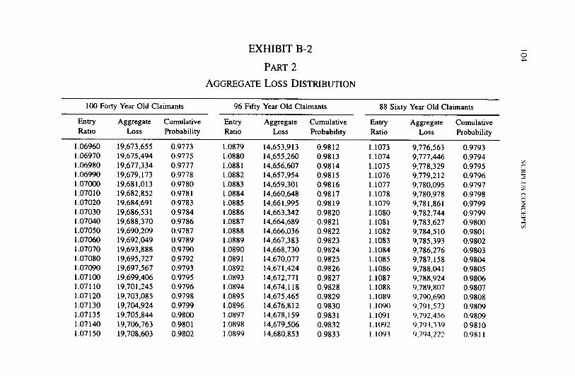
EXHIBIT B-2

PART 2








1.06960 19,673,655 0.9773 1.06970 19,675,494 0.9775 1.06980 19,677,334 0.9777 1.06990 19,679,173 0.9778 1.07000 19,681,013 0.9780 1.07010 19,682,852 0.9781 1.07020 19,684,691 0.9783 1.07030 19,686,531 0.9784 1.07040 19,688,370 0.9786 1.07050 19,690,209 0.9787 1.07060 19,692,049 0.9789 1.07070 19,693,888 0.9790 1.07080 19,695,727 0.9792 1.07090 19,697,567 0.9793 1.07100 19,699,406 0.9795 1.07110 19,701,245 0.9796 1.07120 19,703,085 0.9798 1.07130 19,704,924 0.9799 1.07135 19,705,844 0.9800 1.07140 19,706,763 0.9801 1.07150 19,708,603 0.9802

1.0879 14,653,913 0.9812 1.0880 14,655,260 0.9813 1.0881 14,656,607 0.9814 1.0882 14,657,954 0.9815 1.0883 14,659,301 0.9816 1.0884 14,660,648 0.9817 1.0885 14,661,995 0.9819 1.0886 14,663,342 0.9820 1.0887 14,664,689 0.9821 1.0888 14,666,036 0.9822 1.0889 14,667,383 0.9823 1.0890 14,668,730 0.9824 1.0891 14,670,077 0.9825 1.0892 14,671,424 0.9826 1.0893 14,672,771 0.9827 1.0894 14,674,118 0.9828 1.0895 14,675,465 0.9829 1.0896 14,676,812 0.9830 1.0897 14,678,159 0.9831 1.0898 14,679,506 0.9832 1.0899 14,680,853 0.9833

1.1073 9,776,563 0.9793 1.1074 9,777,446 0.9794 1.1075 9,778,329 0.9795 1.1076 9,779,212 0.9796 1.1077 9,780,095 0.9797 1.1078 9,780,978 0.9798 1.1079 9,781,861 0.9799 1.1080 9,782,744 0.9799 1.1081 9,783,627 0.9800 1.1082 9,784,510 0.9801 1.1083 9,785,393 0.9802 1.1084 9,786,276 0.9803 1.1085 9,787,158 0.9804 1.1086 9,788,041 0.9805 1.1087 9,788,924 0.9806 1.1088 9,789,807 0.9807 1.1089 9,790,690 0.9808 1.1090 9.791,573 0.9809 1.1091 9,792,456 0.9809 1.1092 9,793,339 0.9810 1.1093 9,7(14,222 0.9811

7~

o z

EXHIBIT B-2

PART 3








1.07160 19,710,442 0.9803 1.07170 19,712,281 0.9805 1.07180 19,714,121 0.9806 1.07190 19,715,960 0.9808 1.07200 19,717,799 0.9809 1.07210 19,719,639 0.9810 1.07220 19,721,478 0.9812 1.07230 19,723,318 0.9813 1.07240 19,725,157 0.9814 1.07250 19,726,996 0.9816 1.07260 19,728,836 0.9817 1.07270 19,730,675 0.9818 1.07280 19,732,514 0.9820 1.07290 19,734,354 0.9821 1.07300 19,736,193 0.9822

1.0900 14,682,200 0.9834 1.0901 14,683,547 0.9835 1.0902 14,684,894 0.9836 1.0903 14,686,241 0.9837 1.0904 14,687,588 0.9838 1.0905 14,688,935 0.9839 1.0906 14,690,282 0.9840 1.0907 14,691,629 0.9841 1.0908 14,692,976 0.9842 1.0909 14,694,323 0.9843 1.0910 14,695,670 0.9844 1.0911 14,697,017 0.9845 1.0912 14,698,364 0.9846 1.0913 14,699,711 0.9846 1.0914 14,701,058 0.9847

1.1094 9,795,105 0.9812 1.1095 9,795,988 0.9813 1.1096 9,796,871 0.9814 1.1097 9,797,754 0.9815 1.1098 9,798,636 0.9816 1.1099 9,799,519 0.9816 1.1100 9,800,402 0.9817 1.1200 9,888,694 0.9887 1.1300 9,976,986 0.9933 1.1400 10,065,278 0.9961 1.1500 10,153,570 0.9978 1.1600 10,241,862 0.9988 1.1700 10,330,154 0.9994 1.1800 10,418,446 0.9997 1.1900 10,506,738 0.9999

-'0

©

Q

Surplus—Concepts, Measures of Return, and Determination

Documents

Transcript of Surplus—Concepts, Measures of Return, and Determination