Surge and Swab Pressure CalculationCalculation of Surge and Swab Pressure

Changes in Laminar and Turbulent Flow

While Circulating Mud and Pumping

Andreas Grav Karlsen

Petroleum Geoscience and Engineering

Supervisor: Pål Skalle, IPT

Department of Petroleum Engineering and Applied Geophysics

Submission date: May 2014

Norwegian University of Science and Technology

1

Sammendrag

Verdens energibehov er raskt økende, og avhengigheten av olje- og gass sektoren blir stadig større

for å møte dette behovet. Dette fører til en stadig økende petroleumsaktivitet rundt om i verden. Det

har blitt sagt at alle de enkle brønnene har blitt boret, og at vi kun at utfordrende brønner igjen.

Industrien møter samtidig økonomiske hindre, og «nedetid» er et av de mest kostbare. [Schubert,

Jan 2010] Problemer kan være smale pore/oppsprekking- trykk, borehulls stabilitet, tømte

formasjoner, og formasjonsskade.

Trykkendinger som resultat av Surge og Swab har i mange år blitt sett på med stor bekymring innen

olje og gass industrien. Dersom trykkendringene blir for store kan det resultere i at formasjonen

sprekker opp og innstrømning av formasjonsvæske i brønnen. Dette kan lede til kick, som i verste fall

ender opp i en utblåsning. En utblåsning er det verst tenkelige scenariet, da dette kan lede til store

økonomiske tap og sette menneskeliv i fare.

Denne oppgaven fokuserer på bakgrunns teori og utvikling av et program for å kalkulere

trykkendringer i både laminær og turbulent strømning i «non-newtonian» fluider. Programmet lar

deg velge hvilke sesjoner av brønnen som er ønskelige å studere, samt utregninger av ECD.

Oppgaven vil vise en utledning for en laminær modell, samt en turbulent modell som program et

basert på. Den laminære modellen er videreutviklet fra Brooks modell fra 1982, og den turbulente

modellen er hentet fra en utgivelse fra blant annet Saasen (2012). Programmet er testet opp mot en

sensitivitetsanalyse for å få en mer grundig indikasjon på hvilke parametere som er viktigst.

Programmet er dessverre ikke testet opp mot boredata da dette ikke har vært tilgjengelig.

Resultatene presentert i denne oppgaven er realistiske og gir en god indikasjon på hvilke

trykkendringer som kan forventes. Programmet er brukervennlig og lett å håndtere. Det er viktig å

håndtere de forskjellige parameterne som påvirker trykkedringene. Hastigheten under heise- eller

senke operasjoner er viktige å kontrollere siden trykkendringene endres raskt som resultat av endret

hastighet. Ved høy hastighet vil trykkendringene stige raskt. Brønnhullsgeometri er og en viktig

faktor. Med et økt areal for strømningen synker trykk endringene.

Det er observert at den laminære strømningen avhenger av blant annet «Flow behavior» indeksen n

og «Power Law» konstanten K. Analysen i denne oppgaven viser at dersom «Flow behavior»

2

indeksen synker under en verdi på 0,5 stiger trykket raskt. Trykker øker med synkende «Power Law»

konstant K.

For turbulent strømning observeres det at trykket stiger eksponentielt med økende hastighet. Dette

understreker viktigheten av å utføre heise- og senkeoperasjoner med riktig hastighet. Lengden på

seksjonen gir en lineær endring av trykket.

For fremtidig arbeid vil det være av stor relevans å få testet modellen mot mer boredata fra

industrien. Det har vært krevende å få tilgang på boredata for å teste modellen tilstrekkelig, da flere

selskaper hemmeligholder sine bore rapporter.

3

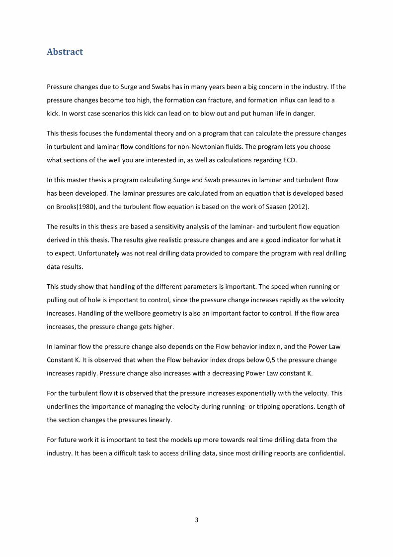
Abstract

Pressure changes due to Surge and Swabs has in many years been a big concern in the industry. If the

pressure changes become too high, the formation can fracture, and formation influx can lead to a

kick. In worst case scenarios this kick can lead on to blow out and put human life in danger.

This thesis focuses the fundamental theory and on a program that can calculate the pressure changes

in turbulent and laminar flow conditions for non-Newtonian fluids. The program lets you choose

what sections of the well you are interested in, as well as calculations regarding ECD.

In this master thesis a program calculating Surge and Swab pressures in laminar and turbulent flow

has been developed. The laminar pressures are calculated from an equation that is developed based

on Brooks(1980), and the turbulent flow equation is based on the work of Saasen (2012).

The results in this thesis are based a sensitivity analysis of the laminar- and turbulent flow equation

derived in this thesis. The results give realistic pressure changes and are a good indicator for what it

to expect. Unfortunately was not real drilling data provided to compare the program with real drilling

data results.

This study show that handling of the different parameters is important. The speed when running or

pulling out of hole is important to control, since the pressure change increases rapidly as the velocity

increases. Handling of the wellbore geometry is also an important factor to control. If the flow area

increases, the pressure change gets higher.

In laminar flow the pressure change also depends on the Flow behavior index n, and the Power Law

Constant K. It is observed that when the Flow behavior index drops below 0,5 the pressure change

increases rapidly. Pressure change also increases with a decreasing Power Law constant K.

For the turbulent flow it is observed that the pressure increases exponentially with the velocity. This

underlines the importance of managing the velocity during running- or tripping operations. Length of

the section changes the pressures linearly.

For future work it is important to test the models up more towards real time drilling data from the

industry. It has been a difficult task to access drilling data, since most drilling reports are confidential.

4

Preface

This master thesis was written in my final semester of my Petroleum Engineering Master Program at

the Norwegian University of Science and Technology.

First of all I want to thank my supervisor Associate Professor Pål Skalle for making it possible for me

to work on this exciting topic. Thank you for your guidance, feedback and great discussions both on

my project and on my master thesis. Also a great thanks to National Oilwell Varo for providing useful

data for the testing of my program.

Thanks to my father, Egil and my mother Lisbeth for the great encouragement and support during my

studies her at NTNU.

To all my friends that have made my time here in Trondheim fantastic, thank you for great memories

and good stories. Special thanks to my housemate and fellow student Asgeir for good discussions and

always being positive.

Andreas Grav Karlsen

Trondheim, Mai 2014

5

Contents

Sammendrag ........................................................................................................................................... 1

Abstract ................................................................................................................................................... 3

Preface ..................................................................................................................................................... 4

List of figures: .......................................................................................................................................... 7

Introduction ............................................................................................................................................. 8

2. Published knowledge on Surge and Swab ......................................................................................... 10

2.1 Definitions of different parameters ............................................................................................ 11

2.2 Rheology ...................................................................................................................................... 17

2.3 Mud pumps ................................................................................................................................. 23

2.4 Problems related to Surge and Swab .......................................................................................... 25

2.4.1 Fluid Influx ............................................................................................................................ 25

2.4.2 Lost Circulation ..................................................................................................................... 26

2.4.3 Kick ....................................................................................................................................... 27

2.4.4 Heave Motion ....................................................................................................................... 29

2.4.5 Equivalent Circulated Density .............................................................................................. 30

2.4.6 Cling factor ........................................................................................................................... 31

2.5 Published methods on estimating Surge and Swab .................................................................... 32

2.5.1 Method 1 – Wellbore Pressure Surges Produced by Pipe Movement ................................. 32

2.5.2 Method 2 – Dynamic Surge/Swab Pressure Predictions ...................................................... 32

2.5.3 Method 3 – A Medium-Order Flow Model for Dynamic Pressure Surges in Tripping

Operations ..................................................................................................................................... 33

2.5.4 Method 4 – Surge and Swab Pressure Predictions for Yield-Power-Law Drilling fluids ....... 34

3 The Selected Models .......................................................................................................................... 35

3.1 –Surge and Swab – laminar pressure model ............................................................................... 35

3.2 Surge and swab – turbulent pressure calculations ..................................................................... 41

4. Test data and sensitivity analysis ...................................................................................................... 42

4.1 Drilling data ................................................................................................................................. 42

4.2 Sensitivity analysis for laminar flow ............................................................................................ 43

4.3 Sensitivity analysis for turbulent flow ......................................................................................... 44

5. Program ............................................................................................................................................. 46

6. Results ............................................................................................................................................... 50

6.1 Laminar flow sensitivity analysis ................................................................................................. 50

6

6.2 Turbulent flow sensitivity analysis .............................................................................................. 53

7. Discussion .......................................................................................................................................... 57

7.1 Quality of model .......................................................................................................................... 57

7.2 Quality of data ............................................................................................................................. 57

7.3 Future work ................................................................................................................................. 58

8. Conclusion ......................................................................................................................................... 59

Nomenclature ........................................................................................................................................ 60

Abbreviations ........................................................................................................................................ 61

Reference list: ........................................................................................................................................ 62

Appendix A ............................................................................................................................................ 64

Appendix B ............................................................................................................................................ 69

Appendix C............................................................................................................................................. 75

7

List of figures:

Figure 1:Cleaning beneath the bit, Survey 2014 ................................................................................... 11

Figure 2: Pressure Overview, Survey ..................................................................................................... 13

Figure 3: Wellbore instabilities,Skalle, 2012 ......................................................................................... 14

Figure 4: Mud balance, Survey .............................................................................................................. 15

Figure 5: Description of Newtonian fluids, Survey ................................................................................ 18

Figure 6: Flow Profile, Laminar, Bingham, Skalle 2012 ......................................................................... 18

Figure 7: Rheological models, Skalle, 2012 ........................................................................................... 19

Figure 8: Geometry and velocity profile for flow between two parallel plates, Skalle 2012 ................ 21

Figure 9: Laminar flow ........................................................................................................................... 22

Figure 10: Turbulent vs. Laminar flow, Survey ...................................................................................... 22

Figure 11: Mud pump in system, Skalle 2012 ....................................................................................... 24

Figure 12: Formation influx, Survey ...................................................................................................... 25

Figure 13: Loss of Circulation, Halliburton, 2013 .................................................................................. 27

Figure 14: Kick, Skalle 2012 ................................................................................................................... 27

Figure 15: Heave motion system, Survey 2014 ..................................................................................... 29

Figure 16: Cling Illustration ................................................................................................................... 31

Figure 17: Overview of model ............................................................................................................... 34

Figure 18: Compared results ................................................................................................................. 34

Figure 19: Geometry of wellbore .......................................................................................................... 35

Figure 20: Geometry of wellbore with radiuses, displaced area .......................................................... 36

Figure 21: Moody friction vs roughness, Skalle 2012 ............................................................................ 41

Figure 22: Daily Drilling Report, Internal unpublished document, NOV ............................................... 42

Figure 23: Input data laminar flow, analysis ......................................................................................... 43

Figure 24: Sensitivity analysis laminar flow calculations ....................................................................... 44

Figure 25: Input data turbulent flow, analysis ...................................................................................... 44

Figure 26: Sensitivity analysis turbulent flow calculations .................................................................... 45

Figure 27: Input section for one of six sections ..................................................................................... 46

Figure 28: Pressure change calculations ............................................................................................... 47

Figure 29: Functions of program ........................................................................................................... 47

Figure 30: ECD Calculations ................................................................................................................... 48

Figure 31: Choosing ECD output ............................................................................................................ 48

Figure 32: Flow chart for Program ........................................................................................................ 49

Figure 33: Flow area vs. Pressure loss ................................................................................................... 50

Figure 34: Pressure change vs n ............................................................................................................ 51

Figure 35: Velocity vs. Pressure change ................................................................................................ 52

Figure 36: Length vs Pressure change, Velocity=1m/s .......................................................................... 53

Figure 37: : Length vs Pressure change, Velocity=2m/s ........................................................................ 53

Figure 38: Length vs Pressure change, Velocity=3m/s ......................................................................... 54

Figure 39: Velocity vs Pressure change, L=50m .................................................................................... 54

Figure 40: Velocity vs Pressure change, L=75m .................................................................................... 55

Figure 41: Velocity vs Pressure change, L=100m .................................................................................. 55

Figure 42: Diameter vs Pressure change L=50m, v=1 m/s .................................................................... 56

Figure 43: Diameter vs Pressure Change L=100m, v=1m/s ................................................................... 56

8

Introduction

The world’s energy needs are increasing and the petroleum industry is getting more and more

important for fulfilling this need. This leads to increasing petroleum activity around the world. It has

been stated by many that all the “easy” wells have been drilled and that we only have “difficult”

wells left. Our industry is facing increasing costly incidences of pressure-related nonproductive time [

Schubert, Jan 2010 ]. Problems include narrow pore- or fracture – pressure, windows, wellbore

stability, depleted formations and formation damage. Saving time is more important than ever, since

downtime is so costly. Problems related to surge and swab pressures can lead to a number of costly

drilling problems such as lost circulations due to low formation fracture and fluid kick. An accurate

model is important in planning drilling operations, because in challenging wells the pressure window

is narrow.

When the drill string is run-in-hole with or without mud circulation through the drill string, an

additional bottom hole pressure called “Surge Pressure” is created. If the surge pressure is too high,

the problems the problems stated above may occur. Swab pressure is the reduction in pressure

change in the wellbore. Knowing more about the pressure surges resulting from lowering and raising

the drill sting is important to have a trouble free operation [ Brooks, 1982 ].

Often we have wells with a very narrow mud window, which means that the difference between the

pore pressure and fracture pressure is small. Narrow mud window is often located in deep water

formations. One of the things we need to take in consideration here is the tripping speed. The

tripping process will therefore take longer time, and be more costly. Creating a program that

calculates the pressure changes will therefore be of help, so that we now at what speed the tripping

process should be at.

It is important to take surge and swab pressures in to consideration when looking at wellbore

stability. Accurate calculations of these pressures are important, so that it is know that the pressure

in the wellbore will be within the limits. A high surge pressure can result in fracturing the well

formation, hence lead to lost circulation. If lost circulation occur the hydrostatic pressure can fall,

and again lead to influx of fluids in the formation. This can lead to a kick. When tripping out of the

hole, swabbing can result in a decrease in pressure. This can lead to formation fluids flowing in to the

wellbore and in a worst case scenario result in a blowout.

9

The objective of this thesis is to improve knowledge of surge and swab pressure changes and build a

model that calculates these, focusing on both Bingham and Power Law fluids in laminar- and

turbulent flow. A model is developed to calculate surge and swab pressure changes and the

estimation of ECD. The two models are based on the work of Brooks (1982) and Saasen(2012). Since

no data is available to test the models, a sensitivity analysis is also made to take a closer look at the

different parameters, and how they affect the results.

10

2. Published knowledge on Surge and Swab

Surge and swab pressure is a well-known issue in the oil-industry. In 1934 pressure surges as a result

of swabbing was detected as a potential reason for influx into the wellbore [Cannon, 1934]. Cannon

discussed the problems as “a possible cause of fluid influx, and extreme cases blowouts”. In 1951

Goins linked surge pressures with lost circulation. Surge and swab pressures can cause a change in

the bottom hole pressure, resulting in to high pressure [Burkhardt,1961]. This pressure change is due

to running or tripping the drill string [Brooks, 1982] In 1988 Mitchell published a paper that extended

some of the existing surge and swab models. He compared his results with the data that Burkhardt

used in 1961. He concluded that in shallow wells, inertial forces and friction were the most important

factors, and in deeper wells the compressibility was key. In 2012 a paper by Arild Saasen among

others were presented. In this paper a new model have been developed, and tested up against the

data Burkhardt used. Some of the consequences as a result of surge and swab can be catastrophic

and these are presented later in this project.

11

2.1 Definitions of different parameters

Mud is the common name for drilling fluid.

The mud system in a drilling operation has many important functions. The most important functions

of the mud are described in chapter 2.1.

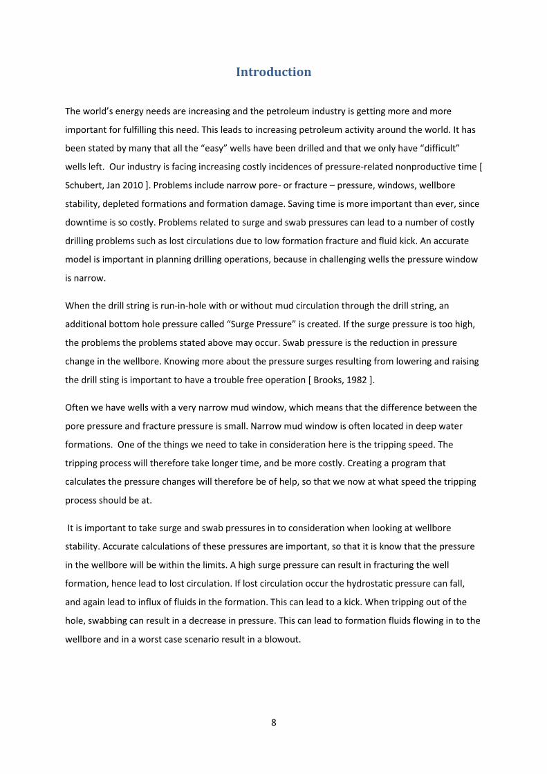
Cleaning beneath the bit:

To maximize the drilling efficiency, the drilling fluid must utilize the hydraulic horsepower from the

main mud pumps to sweep cuttings from the bottom of the hole as soon as they are dislodged and

allow the cutters to continue to be in contact with the formation. If the cuttings are not removed,

they will be ground into smaller particles and adversely affect drilling rate, mud properties, and

project cost. [NOV Confidential, internal unpublished document]

Figure 1:Cleaning beneath the bit, Survey 2014

Carrying drilled out solids from the bottom of the hole to the surface:

When the cuttings have been removed from beneath the drill bit, the fluid must transport them up

towards the surface. Factors which influence movement of the cuttings are the annular velocity, the

size of the cuttings, the cuttings shape, and the properties of the fluid used. [NOV Confidential,

internal unpublished document]

12

Suspending cuttings when circulation is stopped:

Circulation of the drilling fluid is often interrupted to add additional drill pipe, change drill bits,

logging and other operations. The drilling fluids must be able to suspend cuttings and weighting

material while circulation is stopped, but should begin to flow easily when circulation is resumed.

Properties which affect cuttings suspensions are gel strength of the mud, mud density, viscosity and

the density and size of the solids in the mud. [NOV Confidential, internal unpublished document]

Allowing removal of cuttings by the surface system:

Once the mud circulates back to the surface, it is desirable to remove as much of the cuttings as

possible. Most times this is accomplished with mechanical solids control equipment, such as

hydrocyclones, shale shakers and centrifuges. The drilling fluid should be formulated to maximize the

efficiency of the removal equipment, and then return to the tank. [NOV Confidential, internal

unpublished document]

Controlling formation pressure:

The mud column in the wellbore must provide enough hydrostatic pressure to balance formation

pressures and avoid collapse. The hydrostatic pressure is the pressure while the fluid is not being

circulated, at any point in the wellbore depends on the depth and the density of the drilling mud. The

formula used to the hydrostatic pressure is:

* g * h (1)

Where P is the pressure, rho is the density in kg/m3, g is the gravity and h is the vertical depth.

We also have to consider the circulation of the drilling fluid affects the pressure in the wellbore. The

flow of fluid through the annulus exerts additional pressure. The total pressure at any point in the

wellbore is the sum of the hydrostatic pressure and the pressure required to maintain circulation at

that point. The total pressure is often expressed as ECD, the Equivalent Circulating pressure Density.

This is the drilling fluid that would be required to produce the same pressure under static conditions.

[NOV Confidential, internal unpublished document]

ECD is calculated by the following equation:

(2)

[Skalle, 2012 ]

13

ECD and Surge and Swab pressures during tripping and running are very sensitive to the fluid

properties of the drilling fluid. As viscosity increases, ECD and Surge and Swab pressures increase.

Increases in viscosity are caused by chemical imbalances or solid control problems; either an increase

in solid content, or an increase in the concentration of colloidal particles. Also, with higher viscosities

increases frictional pressure loss within the drill string, reducing the hydraulic horsepower available

at the bit. [NOV Confidential, internal unpublished document] [Skalle,2012]

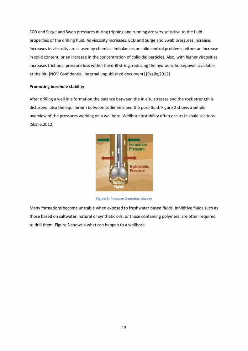
Promoting borehole stability:

After drilling a well in a formation the balance between the in-situ stresses and the rock strength is

disturbed, also the equilibrium between sediments and the pore fluid. Figure 2 shows a simple

overview of the pressures working on a wellbore. Wellbore instability often occurs in shale sections.

[Skalle,2012]

Figure 2: Pressure Overview, Survey

Many formations become unstable when exposed to freshwater based fluids. Inhibitive fluids such as

those based on saltwater, natural or synthetic oils, or those containing polymers, are often required

to drill them. Figure 3 shows a what can happen to a wellbore.

14

Figure 3: Wellbore instabilities,Skalle, 2012

Cooling the drill bit and lubrication the drill string:

Downhole temperatures can exceed 200 degrees centigrade. The contact of the bit with the bottom

of the hole and the rotating drill string with the hole and casing generate additional heat. The drilling

fluid lubricates and cools the points of contact, extending the life of the bit and the drill string. [NOV

Confidential, internal unpublished document]

Helping supporting the drill string:

The fluid in the wellbore exerts a buoyant force on the drill string, reducing the effective weight that

must be suspended from the derrick and handled by the hoisting system. [NOV Confidential, internal

unpublished document]

Allowing accurate information to be obtained for the well:

The drilling fluid must permit electronic logging and not interfere with the analysis of drilled samples.

This helps to control the well, and decreases the possibilities of well problems[NOV Confidential,

internal unpublished document]

Minimizing environmental impact:

The focus on environmental damage has increased rapidly over the last couple of year. Therefore it is

very important that this is taken into consideration when treating the mud. Both the fluid itself and

15

the cuttings generated from the well must be dealt with when drilling is completed. The cuttings may

be contaminated with oil or other chemicals and have to be treated before they can be disposed of.

The base fluid may also be considered a pollutant. Some disposal alternatives are; recycling for future

use, cuttings – re-injections, thermal desorption and stabilization[ NOV Confidential, internal

unpublished document]

Relationship of Fluid Properties:

The ability of a drilling fluid to perform the way we want depends on various fluid properties. Most of

these are measurable and affected by solids control.

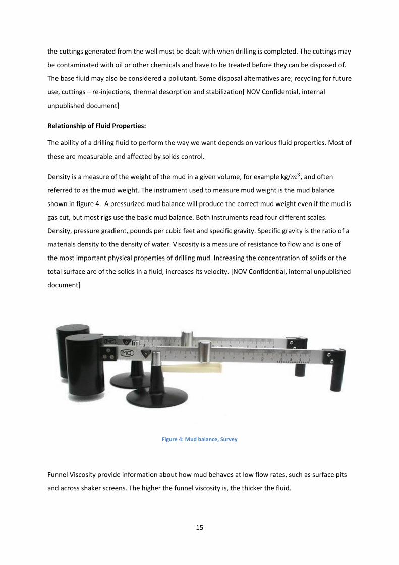
Density is a measure of the weight of the mud in a given volume, for example kg/ , and often

referred to as the mud weight. The instrument used to measure mud weight is the mud balance

shown in figure 4. A pressurized mud balance will produce the correct mud weight even if the mud is

gas cut, but most rigs use the basic mud balance. Both instruments read four different scales.

Density, pressure gradient, pounds per cubic feet and specific gravity. Specific gravity is the ratio of a

materials density to the density of water. Viscosity is a measure of resistance to flow and is one of

the most important physical properties of drilling mud. Increasing the concentration of solids or the

total surface are of the solids in a fluid, increases its velocity. [NOV Confidential, internal unpublished

document]

Figure 4: Mud balance, Survey

Funnel Viscosity provide information about how mud behaves at low flow rates, such as surface pits

and across shaker screens. The higher the funnel viscosity is, the thicker the fluid.

16

Plastic velocity measures the portion of a mud’s flow resistance caused by the mechanical friction

between the suspended particles and by the viscosity of the continuous liquid phase. In practical

terms, plastic viscosity depends on the size, shape and concentration of solid particles in the fluid.

Yield Point is a measure of attractive forces between suspended solid particles in a liquid while it is

being circulated. It measures the positive and negative attractive forces between the solid particles in

a fluid. Yield point is measures with a rotating viscometer and is expressed in lbs/100ft^2. [NOV

Confidential, internal unpublished document]

Filtration or Wall-Cake:

Mud liquid seeps into porous formations leaving a layer of mud solids on the exposed formation

surface. This layer of mud solids is called a filter cake or some places a wall cake. The filter cake forms

a barrier and reduces further filtration out to the formation. This process is referred to as filtration or

fluid losses. [NOV Confidential, internal unpublished document] [Skalle,2012]

Types of drilling fluids:

Drilling fluids are generally categorized as water- and oil- or synthetic-based, in other words,

weighted or unweight muds. Following is a list of typical types of mud.

1. Water-Based-Mud ( WBM )

a. Spud Mud

b. Natural Mud

c. Chemically-Treated Mud

i. Lightly Treated Chemical Mud

ii. Highly Treated Chemical Mud

iii. Low Solids Mud

iv. Polymer Mud ( Non Dispersed Muds )

v. Calcium Treated Mud

vi. Silicate Treated Mud

d. Salt Water Mud

i. Sea Water Mud

ii. Saturated Salt Mud

2. Oil-Based Mud ( OMB ) or Non Aqueous Fluids ( NAFs)

a. Diesel

b. Mineral

c. Synthetic-Base Mud (SBM )

17

i. Olefin

ii. Ester

iii. Others

Water based mud have water as the liquid phase and are used to drill most of the wells in the world

because water is usually available and water based fluids are relatively simple and cheap.

Oil based mud’s or Non Aqueous fluids contain diesel, mineral or synthetic oil as the continuous

liquid phase and are used for wells that require maximum hole protection. NAFs are usually much

more expensive than water based mud’s and therefore are used only when there is a specific need.

NAFs keep the hole in gauge, reducing and minimizing the risk of stuck pipe in crooked or high angle

holes, where hydrate formations are being drilled. [NOV Confidential, internal unpublished

document] [Skalle,2012]

2.2 Rheology

Many different types of fluids are used when drilling, this to maintain the structural integrity of the

borehole, carry out cuttings and to cool the drill bit [Schlumberger Glossary, 2013]. We divide into

Newtonian and non-Newtonian fluids, and in this project non-Newtonian fluids have been taken in

consideration.

Drilling fluids most often behave as non-Newtonian. Non-Newtonian fluids are those in which the

shear stress is not linearly related to the share rate γ. Shear rate expresses the intensity of shearing

action in the pipe, or change of velocity between fluid layers across the flow path:

(3)

The fluids viscosity expresses the resistance to the fluids flow. Viscosity is due to friction between

parcels of the fluid that moves with different velocity. For example honey has a higher viscosity than

water. In Newtonian fluids the viscosity is at a constant level for all shear rates, shown in figure 6,

and a Non-Newtonian fluid is not linearly related to the shear rate. [Skalle,2012]

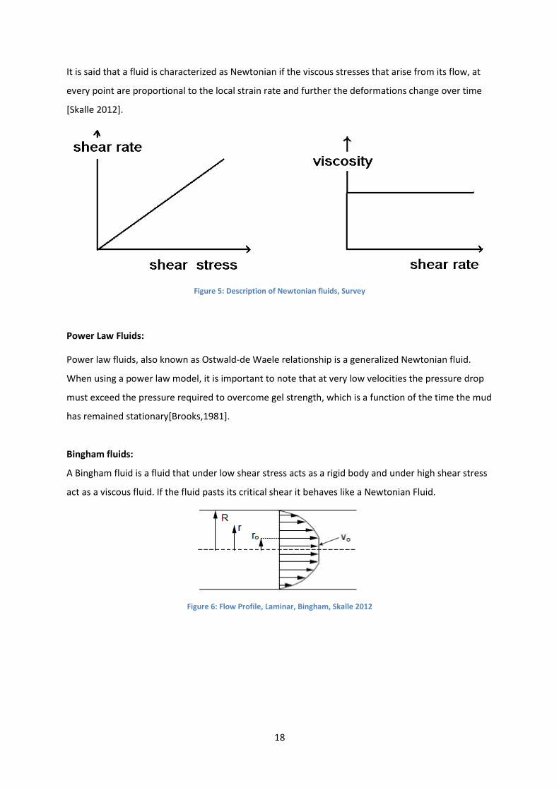
Newtonian Fluids:

The viscosity of a fluid expresses its resistance to the flow. The fluids with a constant viscosity for all

shear rates are called Newtonian.

18

It is said that a fluid is characterized as Newtonian if the viscous stresses that arise from its flow, at

every point are proportional to the local strain rate and further the deformations change over time

[Skalle 2012].

Figure 5: Description of Newtonian fluids, Survey

Power Law Fluids:

Power law fluids, also known as Ostwald-de Waele relationship is a generalized Newtonian fluid.

When using a power law model, it is important to note that at very low velocities the pressure drop

must exceed the pressure required to overcome gel strength, which is a function of the time the mud

has remained stationary[Brooks,1981].

Bingham fluids:

A Bingham fluid is a fluid that under low shear stress acts as a rigid body and under high shear stress

act as a viscous fluid. If the fluid pasts its critical shear it behaves like a Newtonian Fluid.

Figure 6: Flow Profile, Laminar, Bingham, Skalle 2012

19

Rheology of fluids:

Rheology of drilling fluids is measured and determined in the drilling industry by three different

approaches.

2 data points oil field approach ( Fann VG meter )

o It is important to notice that due to the geometry the true shear stress, τw is

obtained by a multiplying factor of 1.06 [Skalle, 2012 ]

o The Fann VG viscometer is suited for the Bingham model.

2 data standard approach

6 data points regression approach

Lately the need for higher quality for rheology has arisen, due to an evolving industry. The

Newtonian model is the simplest model. [Skalle,2012 ]

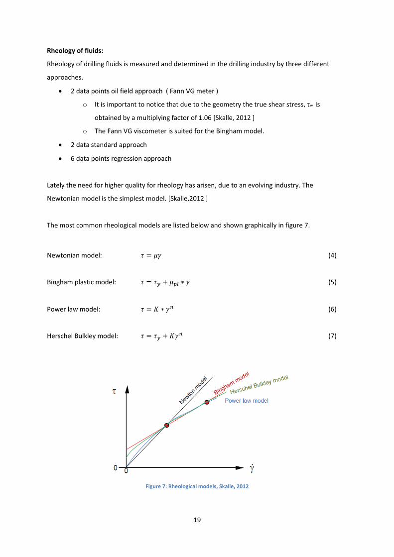
The most common rheological models are listed below and shown graphically in figure 7.

Newtonian model: (4)

Bingham plastic model: (5)

Power law model: (6)

Herschel Bulkley model: (7)

Figure 7: Rheological models, Skalle, 2012

20

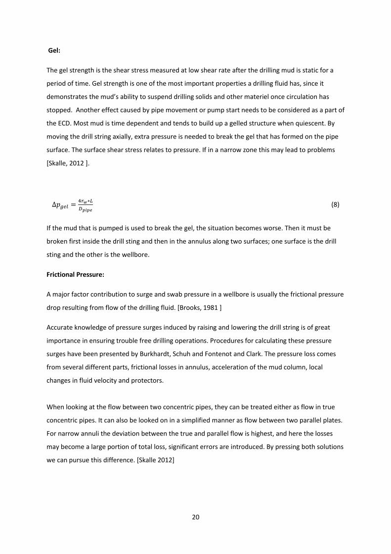
Gel:

The gel strength is the shear stress measured at low shear rate after the drilling mud is static for a

period of time. Gel strength is one of the most important properties a drilling fluid has, since it

demonstrates the mud’s ability to suspend drilling solids and other materiel once circulation has

stopped. Another effect caused by pipe movement or pump start needs to be considered as a part of

the ECD. Most mud is time dependent and tends to build up a gelled structure when quiescent. By

moving the drill string axially, extra pressure is needed to break the gel that has formed on the pipe

surface. The surface shear stress relates to pressure. If in a narrow zone this may lead to problems

[Skalle, 2012 ].

(8)

If the mud that is pumped is used to break the gel, the situation becomes worse. Then it must be

broken first inside the drill sting and then in the annulus along two surfaces; one surface is the drill

sting and the other is the wellbore.

Frictional Pressure:

A major factor contribution to surge and swab pressure in a wellbore is usually the frictional pressure

drop resulting from flow of the drilling fluid. [Brooks, 1981 ]

Accurate knowledge of pressure surges induced by raising and lowering the drill string is of great

importance in ensuring trouble free drilling operations. Procedures for calculating these pressure

surges have been presented by Burkhardt, Schuh and Fontenot and Clark. The pressure loss comes

from several different parts, frictional losses in annulus, acceleration of the mud column, local

changes in fluid velocity and protectors.

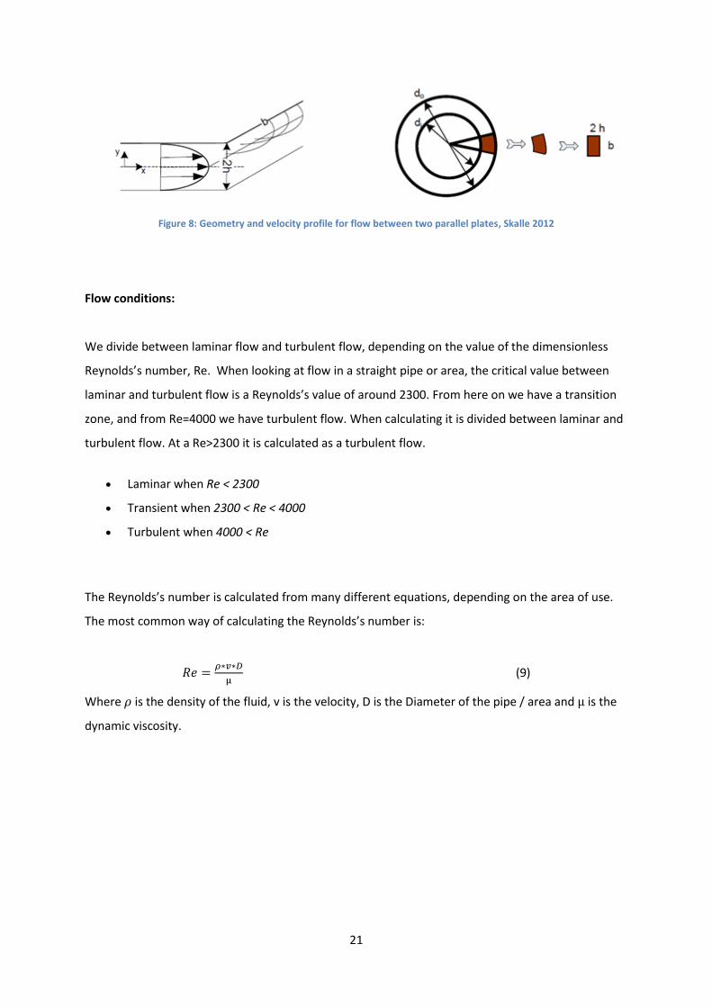
When looking at the flow between two concentric pipes, they can be treated either as flow in true

concentric pipes. It can also be looked on in a simplified manner as flow between two parallel plates.

For narrow annuli the deviation between the true and parallel flow is highest, and here the losses

may become a large portion of total loss, significant errors are introduced. By pressing both solutions

we can pursue this difference. [Skalle 2012]

21

Figure 8: Geometry and velocity profile for flow between two parallel plates, Skalle 2012

Flow conditions:

We divide between laminar flow and turbulent flow, depending on the value of the dimensionless

Reynolds’s number, Re. When looking at flow in a straight pipe or area, the critical value between

laminar and turbulent flow is a Reynolds’s value of around 2300. From here on we have a transition

zone, and from Re=4000 we have turbulent flow. When calculating it is divided between laminar and

turbulent flow. At a Re>2300 it is calculated as a turbulent flow.

Laminar when Re < 2300

Transient when 2300 < Re < 4000

Turbulent when 4000 < Re

The Reynolds’s number is calculated from many different equations, depending on the area of use.

The most common way of calculating the Reynolds’s number is:

(9)

Where is the density of the fluid, v is the velocity, D is the Diameter of the pipe / area and is the

dynamic viscosity.

22

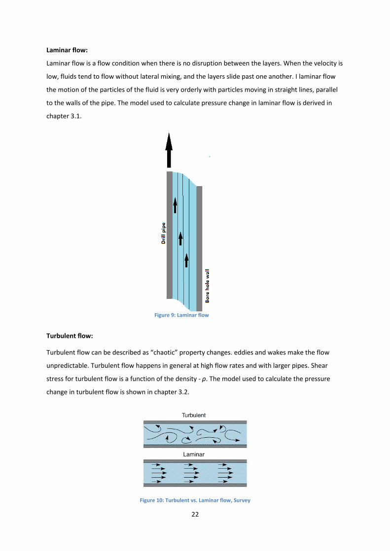
Laminar flow:

Laminar flow is a flow condition when there is no disruption between the layers. When the velocity is

low, fluids tend to flow without lateral mixing, and the layers slide past one another. I laminar flow

the motion of the particles of the fluid is very orderly with particles moving in straight lines, parallel

to the walls of the pipe. The model used to calculate pressure change in laminar flow is derived in

chapter 3.1.

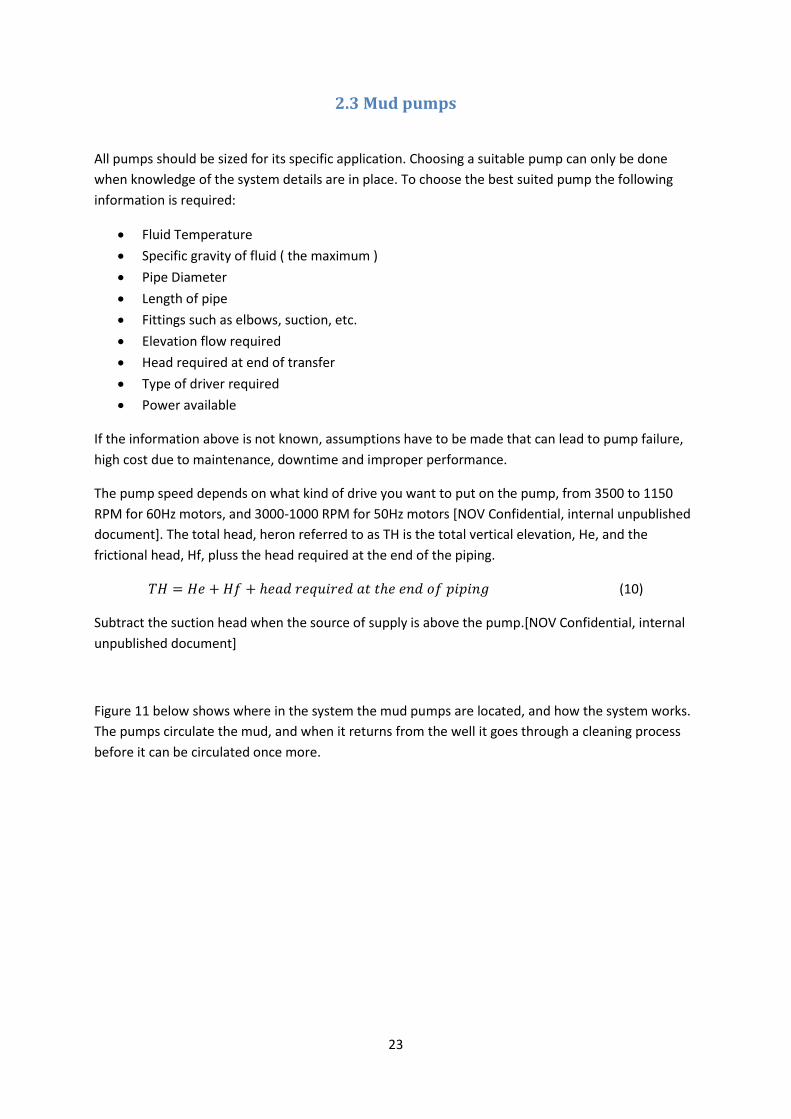
Turbulent flow:

Turbulent flow can be described as “chaotic” property changes. eddies and wakes make the flow

unpredictable. Turbulent flow happens in general at high flow rates and with larger pipes. Shear

stress for turbulent flow is a function of the density - ρ. The model used to calculate the pressure

change in turbulent flow is shown in chapter 3.2.

Figure 10: Turbulent vs. Laminar flow, Survey

Figure 9: Laminar flow

23

2.3 Mud pumps

All pumps should be sized for its specific application. Choosing a suitable pump can only be done

when knowledge of the system details are in place. To choose the best suited pump the following

information is required:

Fluid Temperature

Specific gravity of fluid ( the maximum )

Pipe Diameter

Length of pipe

Fittings such as elbows, suction, etc.

Elevation flow required

Head required at end of transfer

Type of driver required

Power available

If the information above is not known, assumptions have to be made that can lead to pump failure,

high cost due to maintenance, downtime and improper performance.

The pump speed depends on what kind of drive you want to put on the pump, from 3500 to 1150

RPM for 60Hz motors, and 3000-1000 RPM for 50Hz motors [NOV Confidential, internal unpublished

document]. The total head, heron referred to as TH is the total vertical elevation, He, and the

frictional head, Hf, pluss the head required at the end of the piping.

(10)

Subtract the suction head when the source of supply is above the pump.[NOV Confidential, internal

unpublished document]

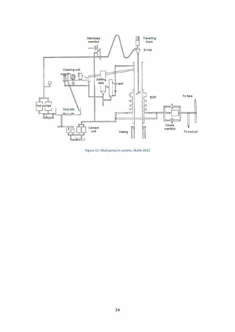
Figure 11 below shows where in the system the mud pumps are located, and how the system works.

The pumps circulate the mud, and when it returns from the well it goes through a cleaning process

before it can be circulated once more.

24

Figure 11: Mud pump in system, Skalle 2012

25

2.4 Problems related to Surge and Swab

Surge and swab can in worst case result in dangerous situations. If the pressure change is too big, the

pressure in the wellbore can get higher than the formation fracture pressure and result in influx of

formation fluids into the wellbore. This can be dangerous knowing that kicks can result in blow outs.

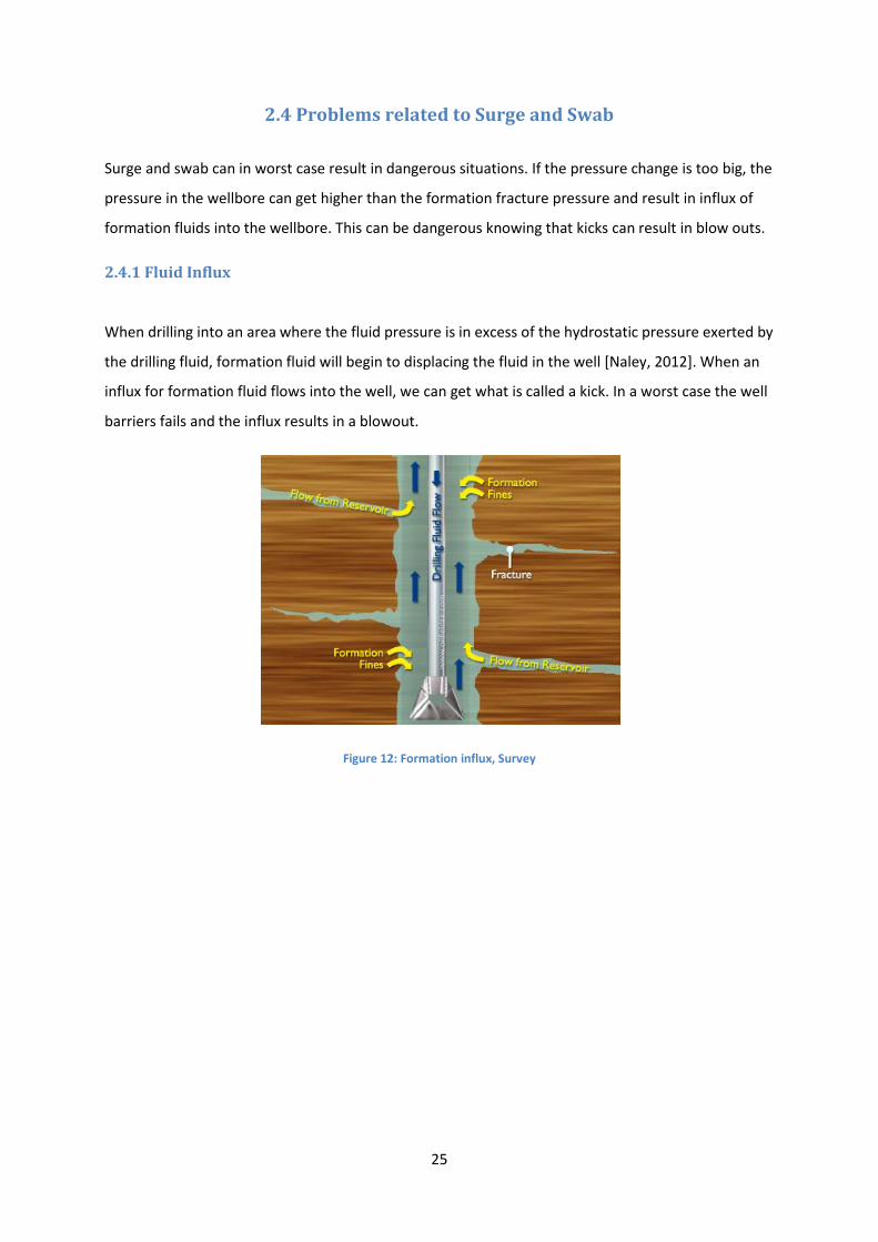
2.4.1 Fluid Influx

When drilling into an area where the fluid pressure is in excess of the hydrostatic pressure exerted by

the drilling fluid, formation fluid will begin to displacing the fluid in the well [Naley, 2012]. When an

influx for formation fluid flows into the well, we can get what is called a kick. In a worst case the well

barriers fails and the influx results in a blowout.

Figure 12: Formation influx, Survey

26

2.4.2 Lost Circulation

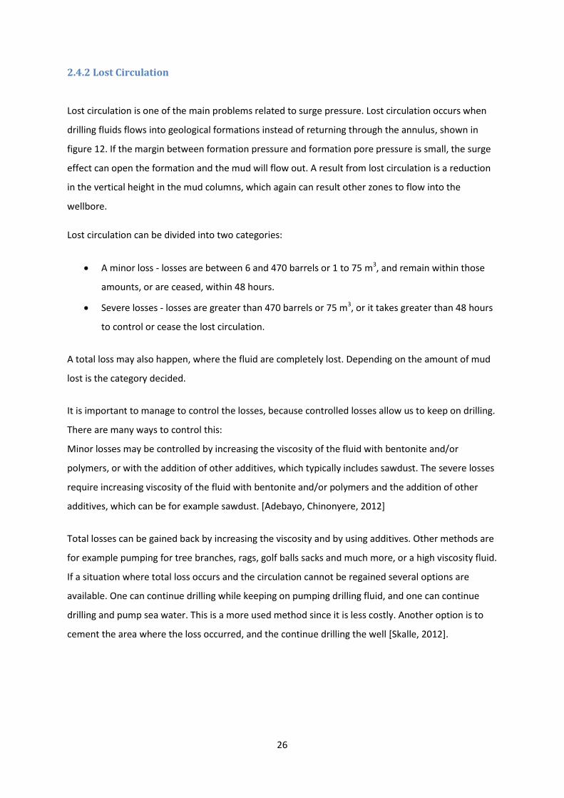
Lost circulation is one of the main problems related to surge pressure. Lost circulation occurs when

drilling fluids flows into geological formations instead of returning through the annulus, shown in

figure 12. If the margin between formation pressure and formation pore pressure is small, the surge

effect can open the formation and the mud will flow out. A result from lost circulation is a reduction

in the vertical height in the mud columns, which again can result other zones to flow into the

wellbore.

Lost circulation can be divided into two categories:

A minor loss - losses are between 6 and 470 barrels or 1 to 75 m3, and remain within those

amounts, or are ceased, within 48 hours.

Severe losses - losses are greater than 470 barrels or 75 m3, or it takes greater than 48 hours

to control or cease the lost circulation.

A total loss may also happen, where the fluid are completely lost. Depending on the amount of mud

lost is the category decided.

It is important to manage to control the losses, because controlled losses allow us to keep on drilling.

There are many ways to control this:

Minor losses may be controlled by increasing the viscosity of the fluid with bentonite and/or

polymers, or with the addition of other additives, which typically includes sawdust. The severe losses

require increasing viscosity of the fluid with bentonite and/or polymers and the addition of other

additives, which can be for example sawdust. [Adebayo, Chinonyere, 2012]

Total losses can be gained back by increasing the viscosity and by using additives. Other methods are

for example pumping for tree branches, rags, golf balls sacks and much more, or a high viscosity fluid.

If a situation where total loss occurs and the circulation cannot be regained several options are

available. One can continue drilling while keeping on pumping drilling fluid, and one can continue

drilling and pump sea water. This is a more used method since it is less costly. Another option is to

cement the area where the loss occurred, and the continue drilling the well [Skalle, 2012].

27

Figure 13: Loss of Circulation, Halliburton, 2013

2.4.3 Kick

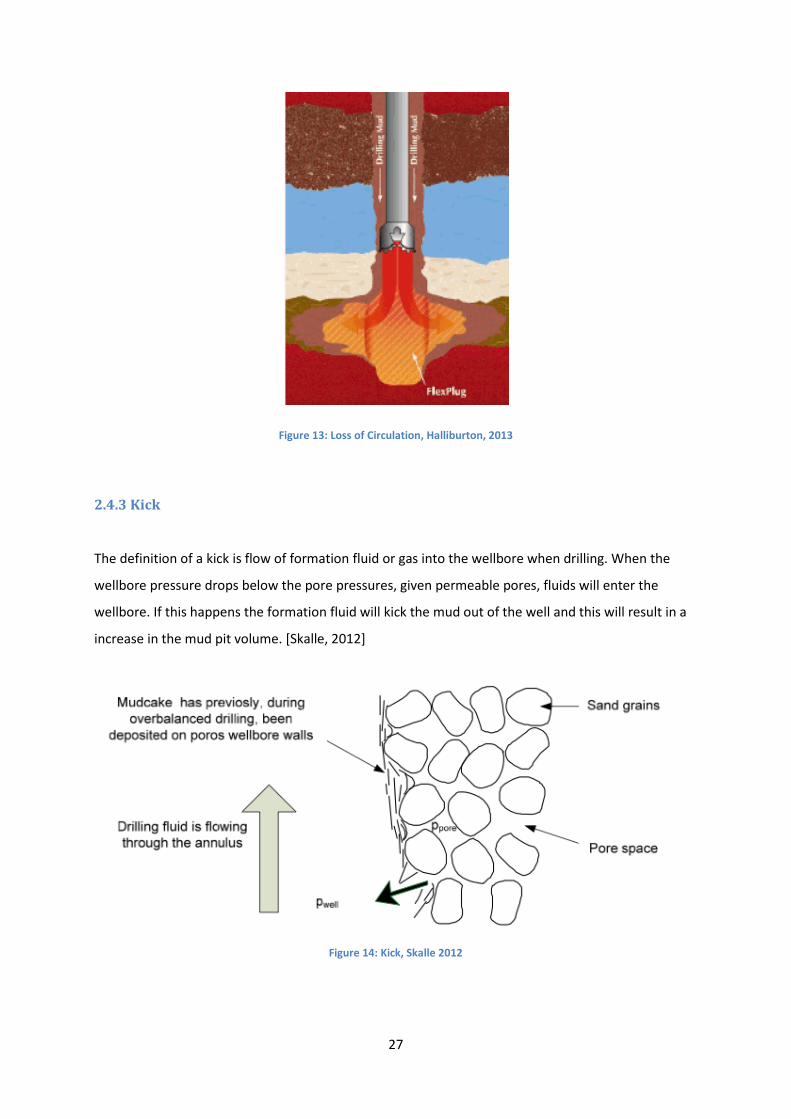
The definition of a kick is flow of formation fluid or gas into the wellbore when drilling. When the

wellbore pressure drops below the pore pressures, given permeable pores, fluids will enter the

wellbore. If this happens the formation fluid will kick the mud out of the well and this will result in a

increase in the mud pit volume. [Skalle, 2012]

Figure 14: Kick, Skalle 2012

28

Kicks can be categorized in two different groups, underbalanced and induced kicks.

Underbalanced kicks are the result of drilling mud weight being insufficient of keeping the formation

fluid at its place. This occurs when drilling through zones where the pore pressure is higher than

expected and the mud is not adjusted to face the higher pore pressure.

Induced kicks are those who occur if dynamic or transient pressure effects lower the pressure in the

well. One example of this is when pulling the drill string out of the well.

In addition to these two one may also experience kick due to hydrate dissociation. [Schlumberger

glossary, 2013]

If a kick is detected it is important to take the proper action to further prevent loss of fluid and

control of the well. Drillers need to be able to predict the gas behavior, because as gas flow up the

wellbore it expands. This can be a great hazard for the people working on the rig, the equipment and

the rig it selves.

In a case where the maximum allowed annular shut-in pressure is higher than the casing pressure,

standard procedure is killing the well. To kill the well a new overbalance in the borehole must be

restored. This is done by pumping mud with a higher density into the wellbore. The two main

methods of doing this is today the Driller’s Method and Engineer’s method.

The Driller’s method is a method where the formation fluid is displaced before injecting the kill mud.

This is the most used method of restoring overbalance, after a kick have been detected. The

Engineer’s method, also called the wait & weight method is a method where the mud weight is

increased and the kill mud is being pumped in immediately. [Skalle, 2012]

When dealing with a kick the proper actions are needed to be made, if not this may in a worst case

lead to a blow out. A blow out is when a uncontrolled flow of reservoir fluid flow into the wellbore.

Underground blowouts are the most difficult to handle. This happens when a reservoir fluid from a

high pressure zone flows into a low pressure zone within the wellbore. It may take months to get

these blowouts under control. A blowout can result in deaths, material damage, environmental

damage and enormous economical losses.

29

2.4.4 Heave Motion

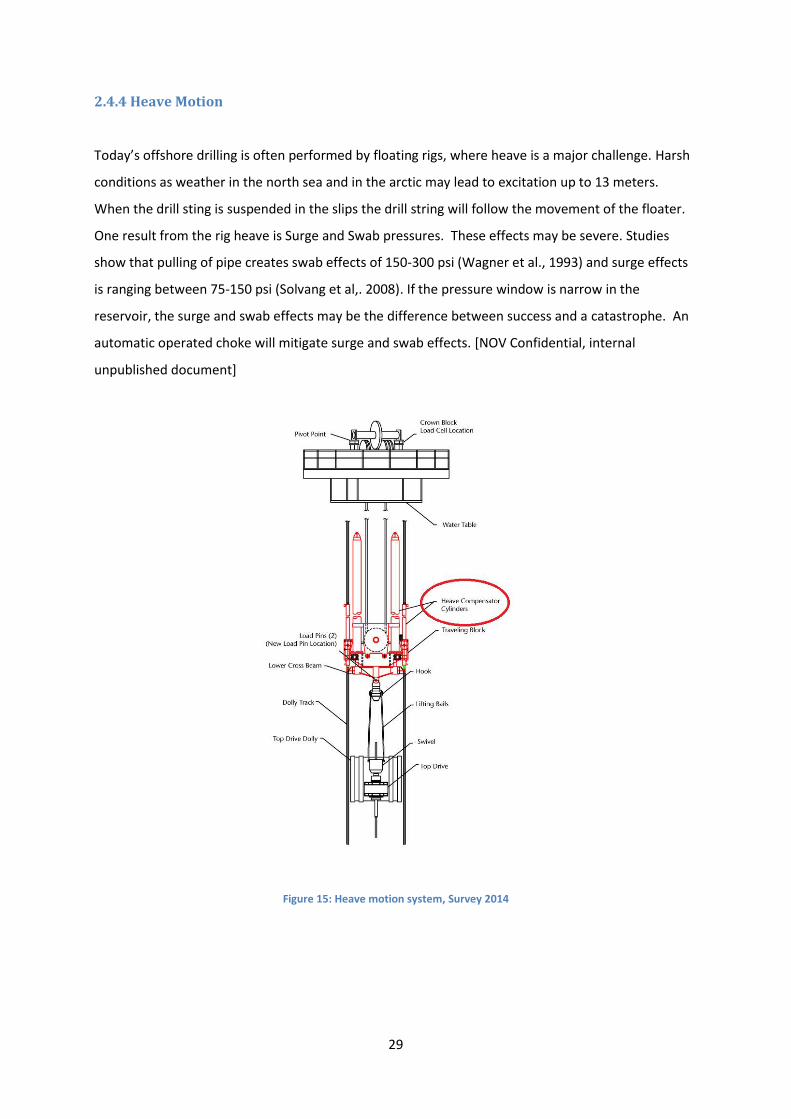
Today’s offshore drilling is often performed by floating rigs, where heave is a major challenge. Harsh

conditions as weather in the north sea and in the arctic may lead to excitation up to 13 meters.

When the drill sting is suspended in the slips the drill string will follow the movement of the floater.

One result from the rig heave is Surge and Swab pressures. These effects may be severe. Studies

show that pulling of pipe creates swab effects of 150‐300 psi (Wagner et al., 1993) and surge effects

is ranging between 75‐150 psi (Solvang et al,. 2008). If the pressure window is narrow in the

reservoir, the surge and swab effects may be the difference between success and a catastrophe. An

automatic operated choke will mitigate surge and swab effects. [NOV Confidential, internal

unpublished document]

Figure 15: Heave motion system, Survey 2014

30

2.4.5 Equivalent Circulated Density

In cases of wells where the pore-fracture window is narrow it is a known fact that managing the

Equivalent Circulated Density, heron referred to as ECD, becomes very important. In these narrow

windows accurate calculations are very important not to allow influx into the wellbore. Calculations

of the ECD are a result of the mud weight, rheological properties and the frictional pressure drop in

the annulus due to solids loading. In addition to these, pressure change due to rotation and Surge &

Swab also must be taken in consideration. It is shown previously that circulated pressure ECD related

problems becomes more accurate when handling extended reach wells, ERD. In high pressure, high

temperature, heron referred to as HPHT, it is show that it becomes very difficult to predict the ECD,

this because the mud properties are difficult to predict. [Resort, Kinabalu 2010] Either way if not

handled properly this may end up in lost circulation or another well control problem.

In the program presented in this thesis calculation of Equivalent Circulated Density is possible at any

section of the well. Equation used in this calculation is taken from Pål Skalle at NTNU.

(2)

As described in the equation above you can see that many factors are to be taken in consideration. In

this thesis the pressure change due to rotation and acceleration are to be neglected, since data on

this have not been provided or found. In future work this should be looked at and taken into

consideration. Z is the length of the section in meters. The parameters can be calculated from these

equations.

31

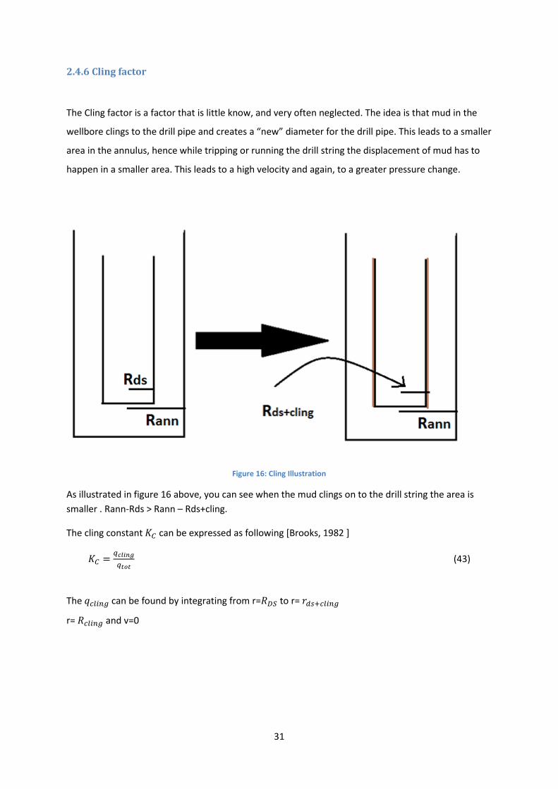
2.4.6 Cling factor

The Cling factor is a factor that is little know, and very often neglected. The idea is that mud in the

wellbore clings to the drill pipe and creates a “new” diameter for the drill pipe. This leads to a smaller

area in the annulus, hence while tripping or running the drill string the displacement of mud has to

happen in a smaller area. This leads to a high velocity and again, to a greater pressure change.

Figure 16: Cling Illustration

As illustrated in figure 16 above, you can see when the mud clings on to the drill string the area is

smaller . Rann-Rds > Rann – Rds+cling.

The cling constant can be expressed as following [Brooks, 1982 ]

(43)

The can be found by integrating from r= to r=

r= and v=0

32

2.5 Published methods on estimating Surge and Swab

There are many methods and publications on the topic surge and swab, and they all have

assumptions that make them different. The following will look at four different methods and

publications.

2.5.1 Method 1 – Wellbore Pressure Surges Produced by Pipe Movement

Burkhardt (1961) was one of the first to try to make a model on surge pressures. In his paper

published in 1961, he compared measured results with those predicted by his theory and showed

that the magnitude of this surge could be predicted. His paper is based upon realistic assumptions,

empirical equations and comparing measured surges to the ones he calculates with his model.

Burkhardt’s model helped calculate the surge and swab pressure for ideal Bingham plastic fluids, and

applied when having a uniform wellbore, with a concentric annulus and steady state flow.

In 1974 Fontenot and Clark published and presented a paper called “An improved method for

calculating surge and swab and circulated pressures in a drilling well”. This was an improvement of

Burckhardt’s work, giving the opportunity to include Power Law fluids as well as Bingham.

2.5.2 Method 2 – Dynamic Surge/Swab Pressure Predictions

R.F. Mitchell’s [1988] presents a dynamic surge and swab model that extends the existing models

with the following four features. The first when pipe and annulus pressures are coupled through the

pipe elasticity, and secondly longitudinal pipe elasticity and fluid viscous forces determine pipe

displacement. Thirdly, fluid properties change as a function of temperature and fourth formation,

pipe and cement elasticity [Mitchell 1988]. Mitchell compared his model and field data to

demonstrate his results. To simulate his model he used the data from Burkhardt and Clark and

Fontenot. He concludes that in shallow wells, inertial forces and friction forces seems to be most

important. Steady flow surge predictions match the peak field pressures well. In deeper wells

Mitchell states that compressibility is important. Steady flow surge models over predict peak

pressures, and the error increases along with the depth. Negative surge pressures are less that in

shallow wells.

33

2.5.3 Method 3 – A Medium-Order Flow Model for Dynamic Pressure Surges in Tripping

Operations

The third publication I have looked at is “A Medium-Order Flow Model for Dynamic Pressure Surges

in Tripping Operations”. The paper was published in 2013 by Kristian Gjerstad from Teknova, Rune

W. Time from UiS and Knut S. Bjørkevoll from SINTEF.

Their model is based ordinary differential equations that predict the surge and swab pressures while

tripping. The model is designed for applications in real-time operations where it is important to

control the pressures. The study is based on a Herschel-Bulkley non-Newtonian fluid. Their model can

automatically adapt uncertain parameters or be calibrated manually. They use simplified flow

equations for the laminar flow regime in drill string and annulus. In the model they chose pressure

variables, P, and the volumetric flow rates Q to be the state variables. Inputs are the string velocity v,

and the inlet pressure P, at the top of the drill string. For normal operations when tripping the only

output is the annular pressure by the bottom hole assembly, and when circulating the flow rate into

the drill string and out of annulus are looked on as outputs.

The annulus between the drill string and the wall of the borehole is divided into n segments. Each

annular segment, j, in the drilling fluid is set to have a uniform pressure, Pj and a volumetric flow

rate, Q. The segments have diameter and inclination . The Bottom hole assembly, or BHA, will

always be the lowest segment, this since it is important to catch the dynamics and friction loss by the

BHA and drill collars.

Conservation of mass in control volume for a compressible fluid is given as:

( ) (11)

Assumptions, the density are a linear function of pressure, and temperature is neglected.

( )

(

( )) (12)

Further they assume that the density is equal in all control volumes.

( )

(

( )) (13)

34

2.5.4 Method 4 – Surge and Swab Pressure Predictions for Yield-Power-Law Drilling fluids

In December 2012 Freddy Crespo, Ahmed, Enfis, Saasen, and Amani published a paper on Surge and

swab pressure predictions.

The paper presents a new steady-state model that can account for fluid and formation

compressibility and pipe elasticity. The paper consider Yield Power Law fluids, YPL.

The performance have been tested by the use of field and laboratory measurements. Comparison of

these models predictions with the measurements showed a good agreement. In most of their cases

the results gives results close to the measurements, this because of their realistic rheology model.

The model is useful when dealing with slimhole, deepwater and ERD drilling applications.

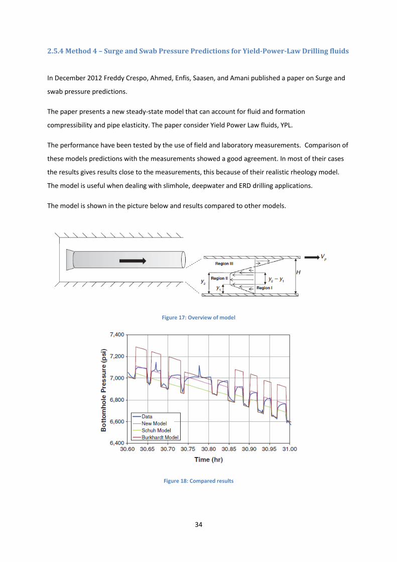
The model is shown in the picture below and results compared to other models.

Figure 17: Overview of model

Figure 18: Compared results

35

3 The Selected Models

To determent the surge and swab pressure loss in laminar flow it has been worked on a model in five

steps. The model is based on a paper from Brooks, A.G., Exploration Logging Inc published in 1982. In

chapter 3.1, Brooks model from 1982 has been further worked on, and developed into a more user-

friendly equation. This model will help develop a program to calculate the laminar pressure changes.

The turbulent flow equation have been obtained from the paper by Freddy Crespo, Ahmed, Enfis,

Saasen, and Amani’s on Surge and swab pressure predictions from 2012. The two equations have

been the base for the program developed to calculate pressure change for different wells.

3.1 –Surge and Swab – laminar pressure model

Following is the derivation of the laminar flow model.

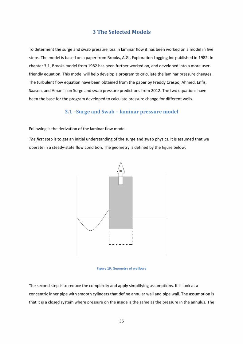
The first step is to get an initial understanding of the surge and swab physics. It is assumed that we

operate in a steady-state flow condition. The geometry is defined by the figure below.

Figure 19: Geometry of wellbore

The second step is to reduce the complexity and apply simplifying assumptions. It is look at a

concentric inner pipe with smooth cylinders that define annular wall and pipe wall. The assumption is

that it is a closed system where pressure on the inside is the same as the pressure in the annulus. The

36

process is in steady state with no fluid acceleration, and Newtonian and Power law fluids are looked

on.

The drill string and fluid are to be seen as elastic. Both pipe elastic and fluid viscous force are a part

of determining the pipe displacement during the tripping procedure, in addition to the formation and

cement elasticity. A result of this is the pressure surge.

There are three terms that are needed to determine the balancing of elastic pipe momentum.

Longitudinal elasticity of pipe + pipe pressure + viscous pipe drag, showed in the equation below.

(14)

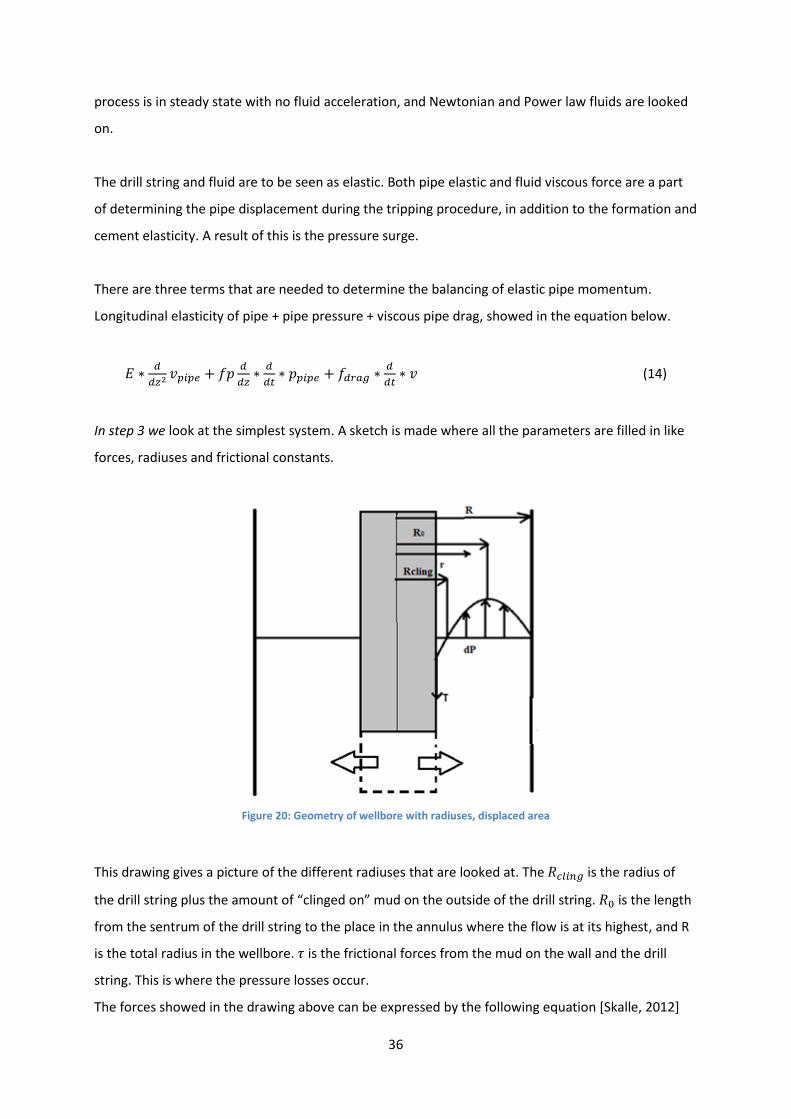
In step 3 we look at the simplest system. A sketch is made where all the parameters are filled in like

forces, radiuses and frictional constants.

Figure 20: Geometry of wellbore with radiuses, displaced area

This drawing gives a picture of the different radiuses that are looked at. The is the radius of

the drill string plus the amount of “clinged on” mud on the outside of the drill string. is the length

from the sentrum of the drill string to the place in the annulus where the flow is at its highest, and R

is the total radius in the wellbore. is the frictional forces from the mud on the wall and the drill

string. This is where the pressure losses occur.

The forces showed in the drawing above can be expressed by the following equation [Skalle, 2012]

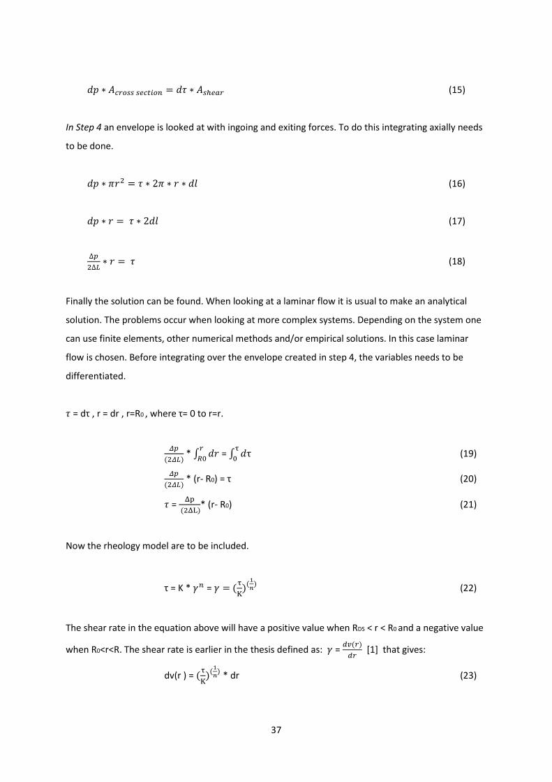
37

(15)

In Step 4 an envelope is looked at with ingoing and exiting forces. To do this integrating axially needs

to be done.

(16)

(17)

(18)

Finally the solution can be found. When looking at a laminar flow it is usual to make an analytical

solution. The problems occur when looking at more complex systems. Depending on the system one

can use finite elements, other numerical methods and/or empirical solutions. In this case laminar

flow is chosen. Before integrating over the envelope created in step 4, the variables needs to be

differentiated.

= dτ , r = dr , r=R0 , where τ= 0 to r=r.

( ) * ∫

= ∫

(19)

( ) * (r- R0) = τ (20)

=

( )* (r- R0) (21)

Now the rheology model are to be included.

τ = K * = (

)(

) (22)

The shear rate in the equation above will have a positive value when RDS < r < R0 and a negative value

when R0<r<R. The shear rate is earlier in the thesis defined as: = ( )

[1] that gives:

dv(r ) = (

)(

) * dr (23)

38

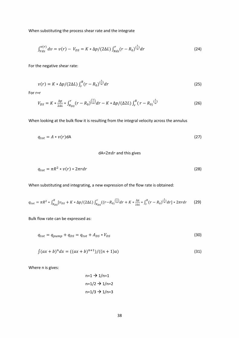
When substituting the process shear rate and the integrate

∫ ( ) ( ) ∫ ( )(

)

( )

(24)

For the negative shear rate:

( ) ( ) ∫ ( )(

)

(25)

For r=r

∫ ( )

(

)

( ) ∫ (

)

(

) (26)

When looking at the bulk flow it is resulting from the integral velocity across the annulus

( ) dA (27)

dA= and this gives

( ) (28)

When substituting and integrating, a new expression of the flow rate is obtained:

∫ ( ) ∫ (( )(

)

∫ ( )

(

)

r (29)

Bulk flow rate can be expressed as:

(30)

∫( ) (( ) ) (( ) ) (31)

Where n is gives:

n=1 1/n=1

n=1/2 1/n=2

n=1/3 1/n=3

39

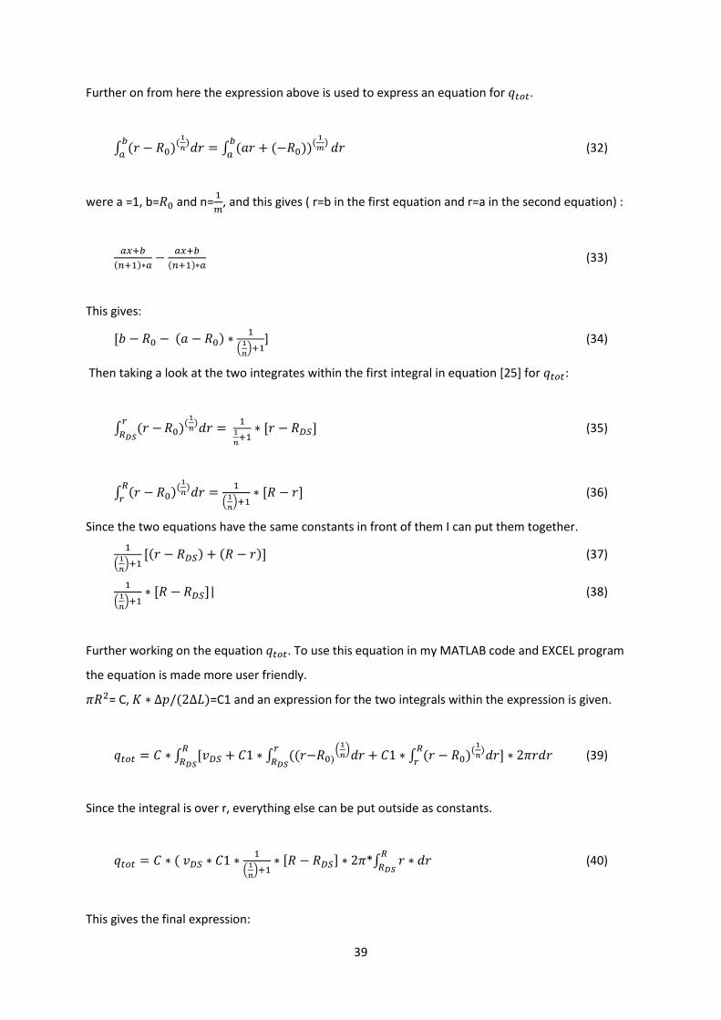
Further on from here the expression above is used to express an equation for .

∫ ( )(

) ∫ ( ( ))

(

)

(32)

were a =1, b= and n=

, and this gives ( r=b in the first equation and r=a in the second equation) :

( )

( ) (33)

This gives:

( )

(

)

] (34)

Then taking a look at the two integrates within the first integral in equation [25] for :

∫ (

)

(

)

(35)

∫ ( )(

)

(

)

(36)

Since the two equations have the same constants in front of them I can put them together.

(

)

( ) ( ) (37)

(

)

| (38)

Further working on the equation . To use this equation in my MATLAB code and EXCEL program

the equation is made more user friendly.

= C, ( )=C1 and an expression for the two integrals within the expression is given.

∫ ∫ (( )(

) ∫ ( )

(

)

(39)

Since the integral is over r, everything else can be put outside as constants.

(

(

)

*∫

(40)

This gives the final expression:

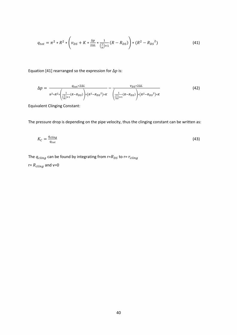
40

(

(

)

( )) ( ) (41)

Equation [41] rearranged so the expression for is:

(

(

) ( )) (

)

(

(

) ( )) (

)

(42)

Equivalent Clinging Constant:

The pressure drop is depending on the pipe velocity, thus the clinging constant can be written as:

(43)

The can be found by integrating from r= to r=

r= and v=0

41

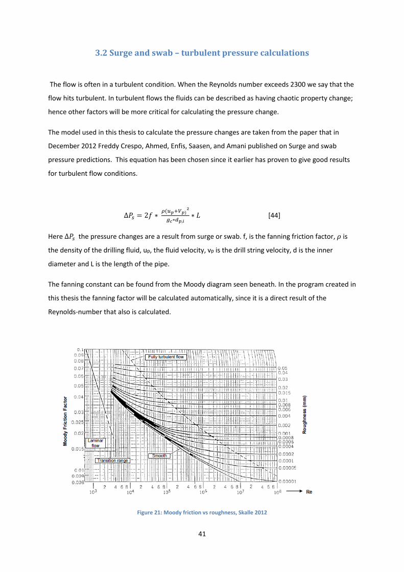
3.2 Surge and swab – turbulent pressure calculations

The flow is often in a turbulent condition. When the Reynolds number exceeds 2300 we say that the

flow hits turbulent. In turbulent flows the fluids can be described as having chaotic property change;

hence other factors will be more critical for calculating the pressure change.

The model used in this thesis to calculate the pressure changes are taken from the paper that in

December 2012 Freddy Crespo, Ahmed, Enfis, Saasen, and Amani published on Surge and swab

pressure predictions. This equation has been chosen since it earlier has proven to give good results

for turbulent flow conditions.

( )

[44]

Here the pressure changes are a result from surge or swab. f, is the fanning friction factor, is

the density of the drilling fluid, up, the fluid velocity, vp is the drill string velocity, d is the inner

diameter and L is the length of the pipe.

The fanning constant can be found from the Moody diagram seen beneath. In the program created in

this thesis the fanning factor will be calculated automatically, since it is a direct result of the

Reynolds-number that also is calculated.

Figure 21: Moody friction vs roughness, Skalle 2012

42

4. Test data and sensitivity analysis

Acquiring good and relevant test data to simulate the results for this program has been challenging.

Few companies are willing to shear their data, but some data has been collected. National Oilwell

Varco has been helpful and provided some drilling data that were used when performing the

sensitivity analysis. Since only some of the data were provided it was not possible to compare the

results.

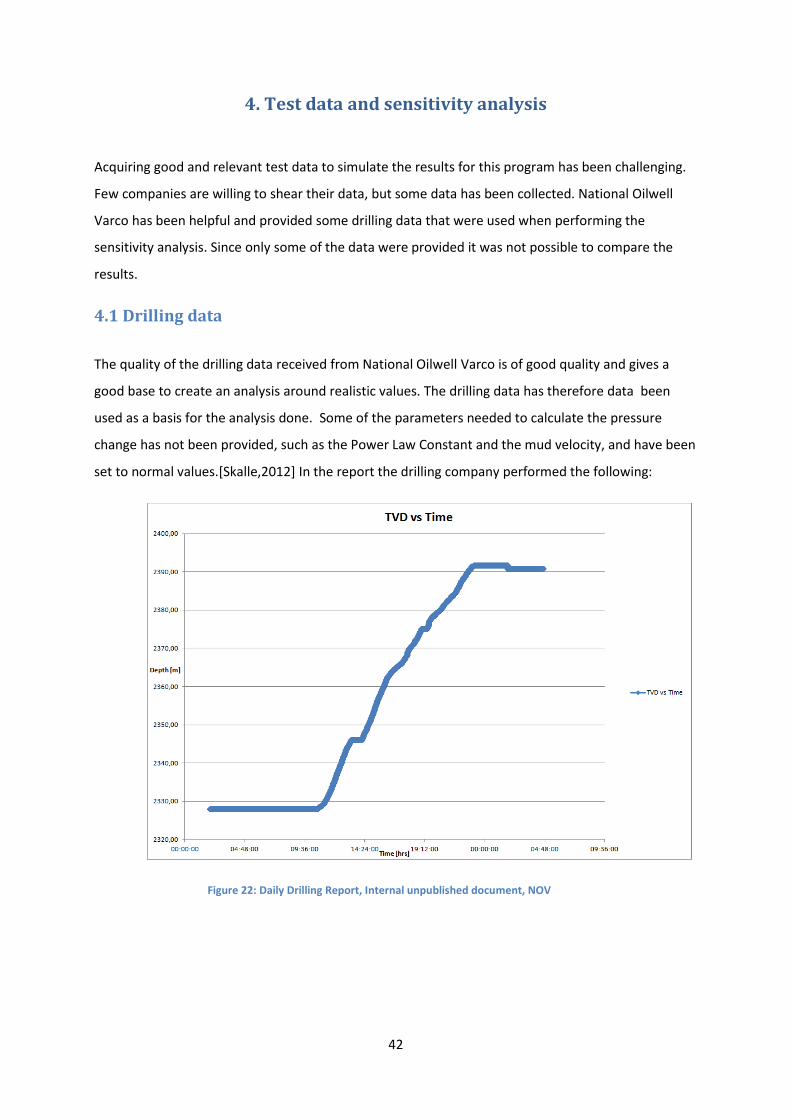
4.1 Drilling data

The quality of the drilling data received from National Oilwell Varco is of good quality and gives a

good base to create an analysis around realistic values. The drilling data has therefore data been

used as a basis for the analysis done. Some of the parameters needed to calculate the pressure

change has not been provided, such as the Power Law Constant and the mud velocity, and have been

set to normal values.[Skalle,2012] In the report the drilling company performed the following:

Figure 22: Daily Drilling Report, Internal unpublished document, NOV

43

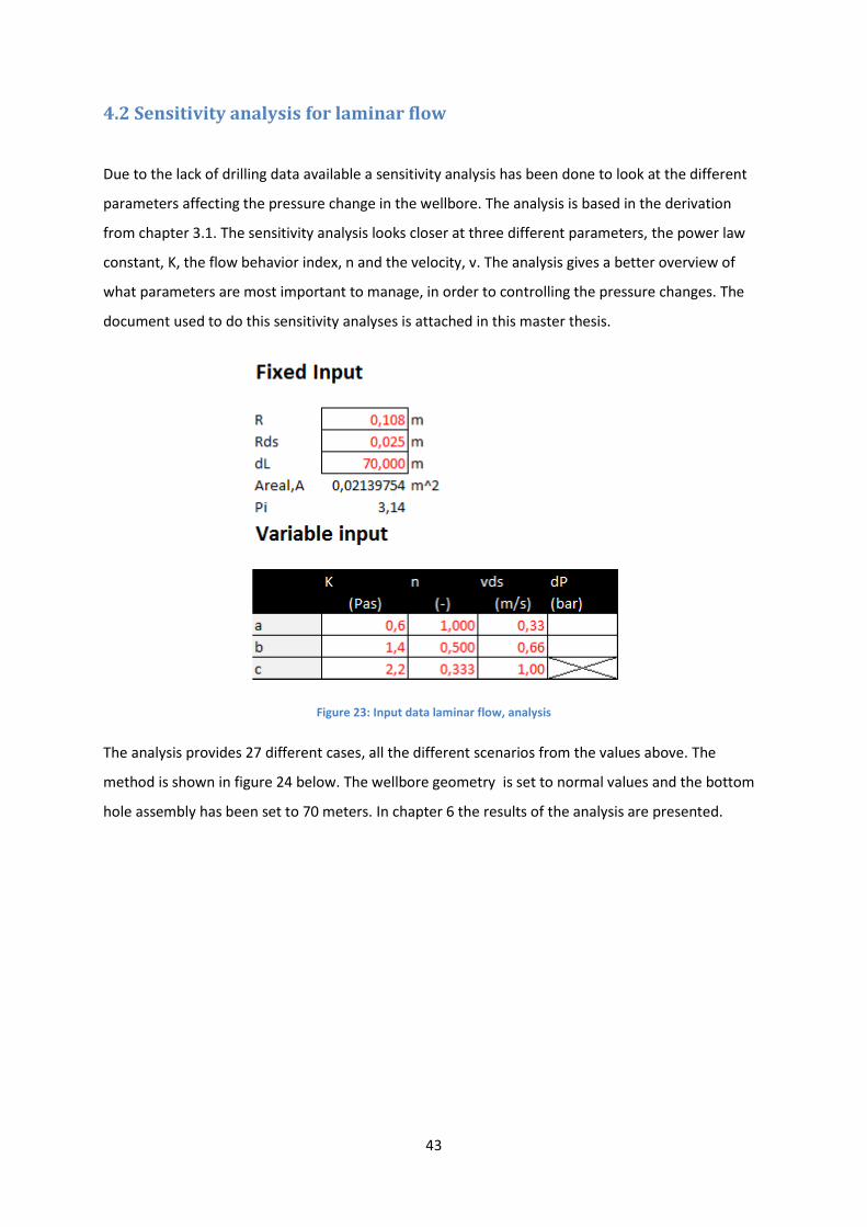
4.2 Sensitivity analysis for laminar flow

Due to the lack of drilling data available a sensitivity analysis has been done to look at the different

parameters affecting the pressure change in the wellbore. The analysis is based in the derivation

from chapter 3.1. The sensitivity analysis looks closer at three different parameters, the power law

constant, K, the flow behavior index, n and the velocity, v. The analysis gives a better overview of

what parameters are most important to manage, in order to controlling the pressure changes. The

document used to do this sensitivity analyses is attached in this master thesis.

Figure 23: Input data laminar flow, analysis

The analysis provides 27 different cases, all the different scenarios from the values above. The

method is shown in figure 24 below. The wellbore geometry is set to normal values and the bottom

hole assembly has been set to 70 meters. In chapter 6 the results of the analysis are presented.

44

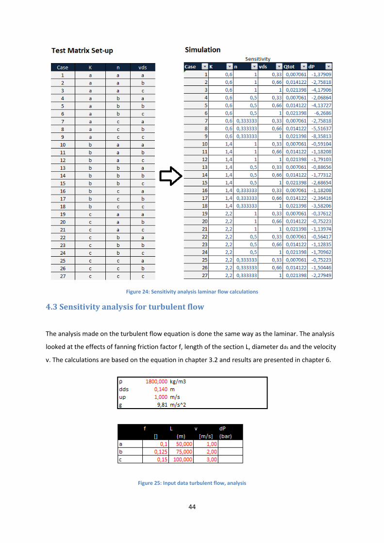
Figure 24: Sensitivity analysis laminar flow calculations

4.3 Sensitivity analysis for turbulent flow

The analysis made on the turbulent flow equation is done the same way as the laminar. The analysis

looked at the effects of fanning friction factor f, length of the section L, diameter dds and the velocity

v. The calculations are based on the equation in chapter 3.2 and results are presented in chapter 6.

Figure 25: Input data turbulent flow, analysis

45

As seen in figure 25 and 26 the input and the parameters tested gives out 27 different cases and

results.

Figure 26: Sensitivity analysis turbulent flow calculations

The calculations are attached.

46

5. Program

The program created in this thesis is an EXCEL based program that calculates the pressure changes in

the wellbore due to surge and swab. The program processes the input data to check if the flow is

laminar or turbulent.

Figure 27: Input section for one of six sections

Further on, the program chooses the pressure change model based on the flow conditions. To

calculate the turbulent pressure change the fanning friction factor is calculated as a result of the

value of the Reynolds number. The calculations are based on the equations shown in Chapter 3. The

picture underneath shows the calculations for pressure change as a result of the input data. Note

that all pictures with calculations in Chapter 5 have example values, and are not linked to the actual

results.

47

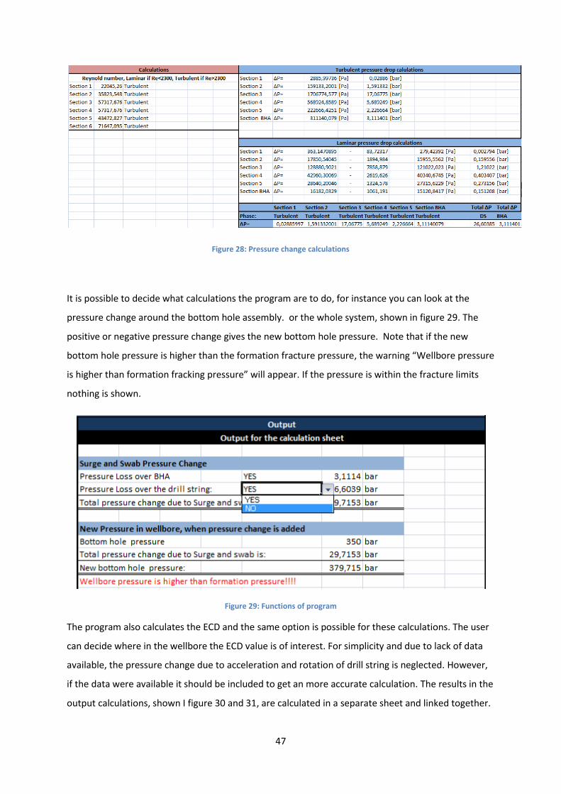
Figure 28: Pressure change calculations

It is possible to decide what calculations the program are to do, for instance you can look at the

pressure change around the bottom hole assembly. or the whole system, shown in figure 29. The

positive or negative pressure change gives the new bottom hole pressure. Note that if the new

bottom hole pressure is higher than the formation fracture pressure, the warning “Wellbore pressure

is higher than formation fracking pressure” will appear. If the pressure is within the fracture limits

nothing is shown.

Figure 29: Functions of program

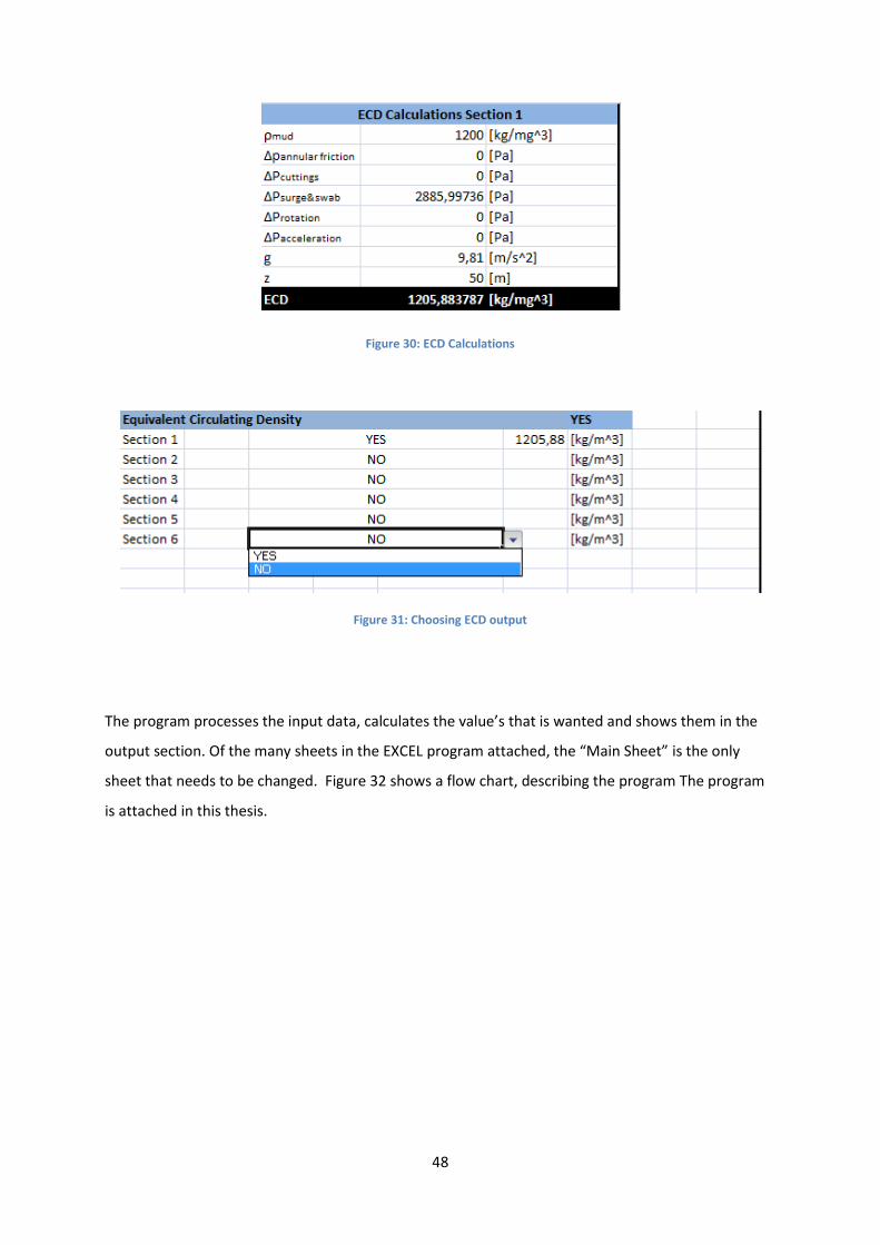
The program also calculates the ECD and the same option is possible for these calculations. The user

can decide where in the wellbore the ECD value is of interest. For simplicity and due to lack of data

available, the pressure change due to acceleration and rotation of drill string is neglected. However,

if the data were available it should be included to get an more accurate calculation. The results in the

output calculations, shown I figure 30 and 31, are calculated in a separate sheet and linked together.

48

Figure 30: ECD Calculations

Figure 31: Choosing ECD output

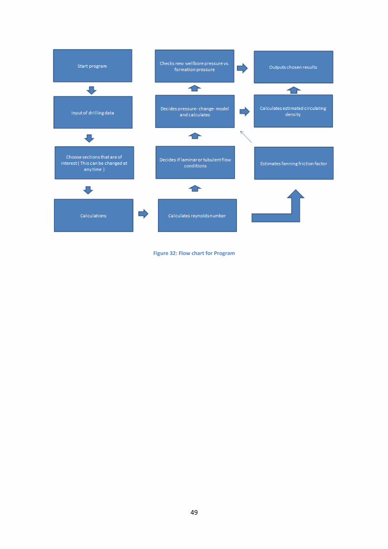
The program processes the input data, calculates the value’s that is wanted and shows them in the

output section. Of the many sheets in the EXCEL program attached, the “Main Sheet” is the only

sheet that needs to be changed. Figure 32 shows a flow chart, describing the program The program

is attached in this thesis.

49

Figure 32: Flow chart for Program

50

6. Results

Due to lack of drilling data sensitivity analysis has been performed to see what parameters are

effecting the pressure change the most. The drilling data that were provided are confidential, so that

it was only possible to use some of the data. In chapter 4.2 and 4.3 the data used in the analysis is

presented. For future work the model should be tested up towards real time drilling data.

6.1 Laminar flow sensitivity analysis

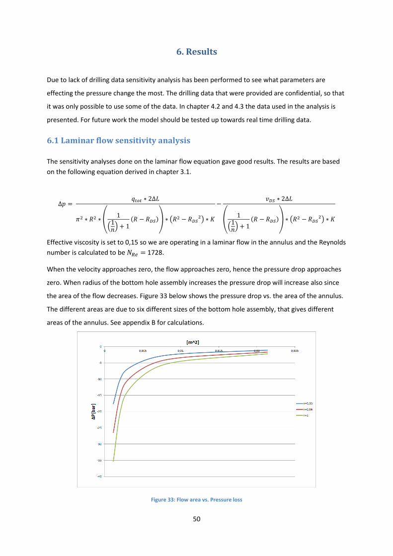
The sensitivity analyses done on the laminar flow equation gave good results. The results are based

on the following equation derived in chapter 3.1.

(

( )

( )) ( )

(

( )

( )) ( )

Effective viscosity is set to 0,15 so we are operating in a laminar flow in the annulus and the Reynolds

number is calculated to be 1728.

When the velocity approaches zero, the flow approaches zero, hence the pressure drop approaches

zero. When radius of the bottom hole assembly increases the pressure drop will increase also since

the area of the flow decreases. Figure 33 below shows the pressure drop vs. the area of the annulus.

The different areas are due to six different sizes of the bottom hole assembly, that gives different

areas of the annulus. See appendix B for calculations.

Figure 33: Flow area vs. Pressure loss

51

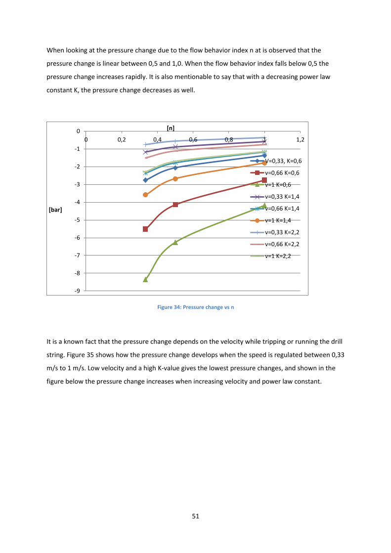
When looking at the pressure change due to the flow behavior index n at is observed that the

pressure change is linear between 0,5 and 1,0. When the flow behavior index falls below 0,5 the

pressure change increases rapidly. It is also mentionable to say that with a decreasing power law

constant K, the pressure change decreases as well.

Figure 34: Pressure change vs n

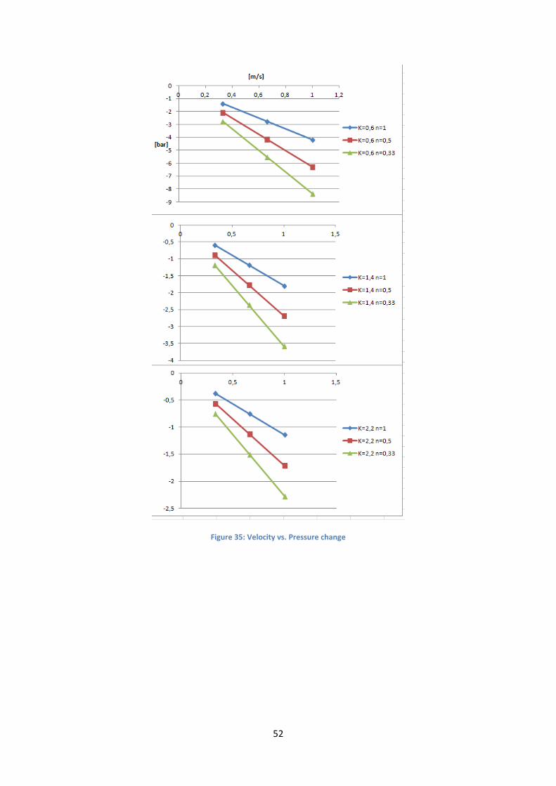
It is a known fact that the pressure change depends on the velocity while tripping or running the drill

string. Figure 35 shows how the pressure change develops when the speed is regulated between 0,33

m/s to 1 m/s. Low velocity and a high K-value gives the lowest pressure changes, and shown in the

figure below the pressure change increases when increasing velocity and power law constant.

-9

-8

-7

-6

-5

-4

-3

-2

-1

0

0 0,2 0,4 0,6 0,8 1 1,2

[bar]

[n]

V=0,33, K=0,6

v=0,66 K=0,6

v=1 K=0,6

v=0,33 K=1,4

v=0,66 K=1,4

v=1 K=1,4

v=0,33 K=2,2

v=0,66 K=2,2

v=1 K=2,2

52

Figure 35: Velocity vs. Pressure change

53

6.2 Turbulent flow sensitivity analysis

The result from the sensitivity analysis on the turbulent flow equation gives good and realistic

results. It is easy to see what parameters that affect the pressure change the most, hence what

parameters that needs to be taken in to consideration when running or tripping.

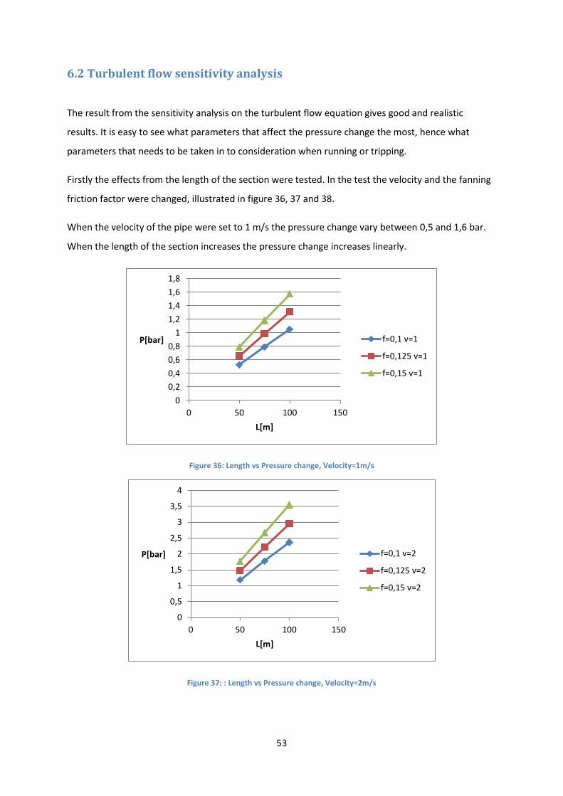
Firstly the effects from the length of the section were tested. In the test the velocity and the fanning

friction factor were changed, illustrated in figure 36, 37 and 38.

When the velocity of the pipe were set to 1 m/s the pressure change vary between 0,5 and 1,6 bar.

When the length of the section increases the pressure change increases linearly.

Figure 36: Length vs Pressure change, Velocity=1m/s

Figure 37: : Length vs Pressure change, Velocity=2m/s

0

0,2

0,4

0,6

0,8

1

1,2

1,4

1,6

1,8

0 50 100 150

P[bar]

L[m]

f=0,1 v=1

f=0,125 v=1

f=0,15 v=1

0

0,5

1

1,5

2

2,5

3

3,5

4

0 50 100 150

P[bar]

L[m]

f=0,1 v=2

f=0,125 v=2

f=0,15 v=2

54

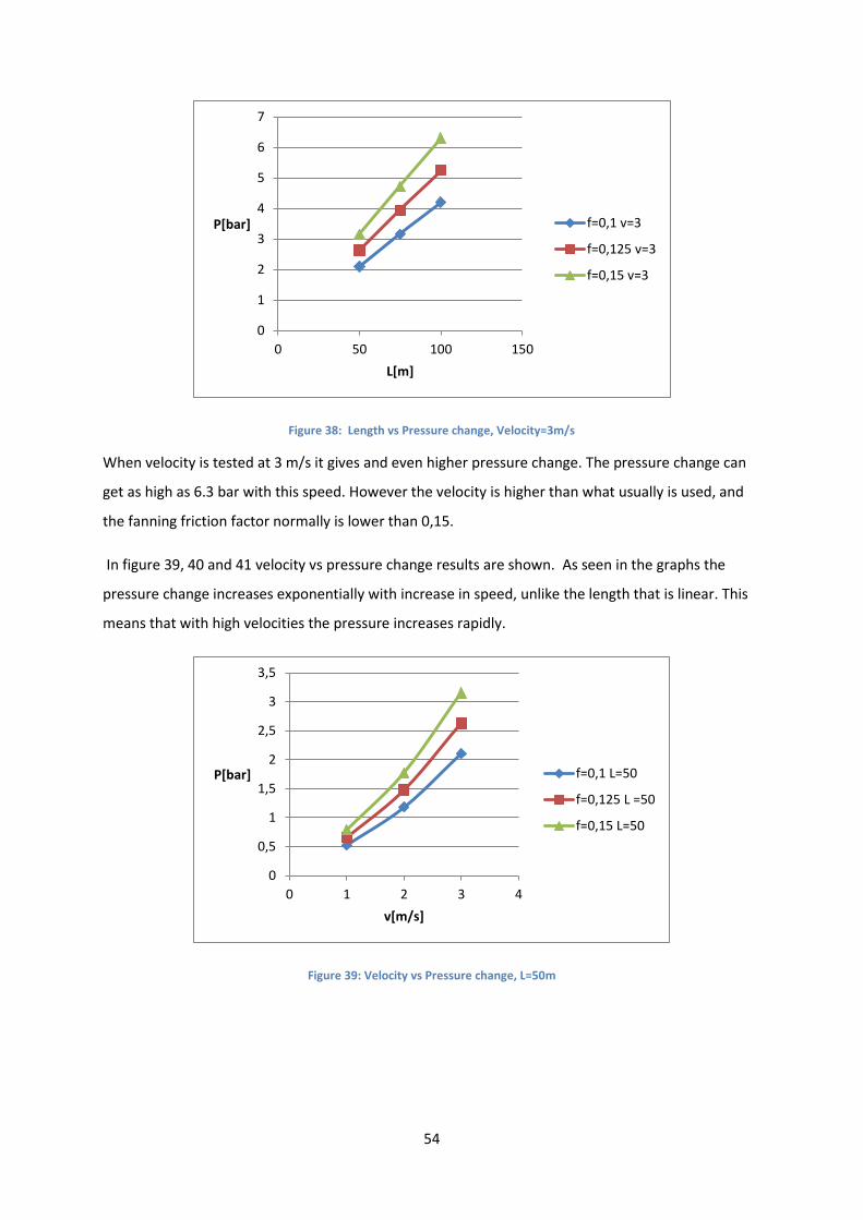
Figure 38: Length vs Pressure change, Velocity=3m/s

When velocity is tested at 3 m/s it gives and even higher pressure change. The pressure change can

get as high as 6.3 bar with this speed. However the velocity is higher than what usually is used, and

the fanning friction factor normally is lower than 0,15.

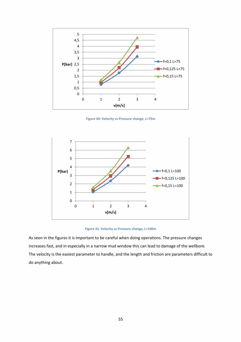
In figure 39, 40 and 41 velocity vs pressure change results are shown. As seen in the graphs the

pressure change increases exponentially with increase in speed, unlike the length that is linear. This

means that with high velocities the pressure increases rapidly.

Figure 39: Velocity vs Pressure change, L=50m

0

1

2

3

4

5

6

7

0 50 100 150

P[bar]

L[m]

f=0,1 v=3

f=0,125 v=3

f=0,15 v=3

0

0,5

1

1,5

2

2,5

3

3,5

0 1 2 3 4

P[bar]

v[m/s]

f=0,1 L=50

f=0,125 L =50

f=0,15 L=50

55

Figure 40: Velocity vs Pressure change, L=75m

Figure 41: Velocity vs Pressure change, L=100m

As seen in the figures it is important to be careful when doing operations. The pressure changes

increases fast, and in especially in a narrow mud window this can lead to damage of the wellbore.

The velocity is the easiest parameter to handle, and the length and friction are parameters difficult to

do anything about.

0

0,5

1

1,5

2

2,5

3

3,5

4

4,5

5

0 1 2 3 4

P[bar]

v[m/s]

f=0,1 L=75

f=0,125 L=75

f=0,15 L=75

0

1

2

3

4

5

6

7

0 1 2 3 4

P[bar]

v[m/s]

f=0,1 L=100

f=0,125 L=100

f=0,15 L=100

56

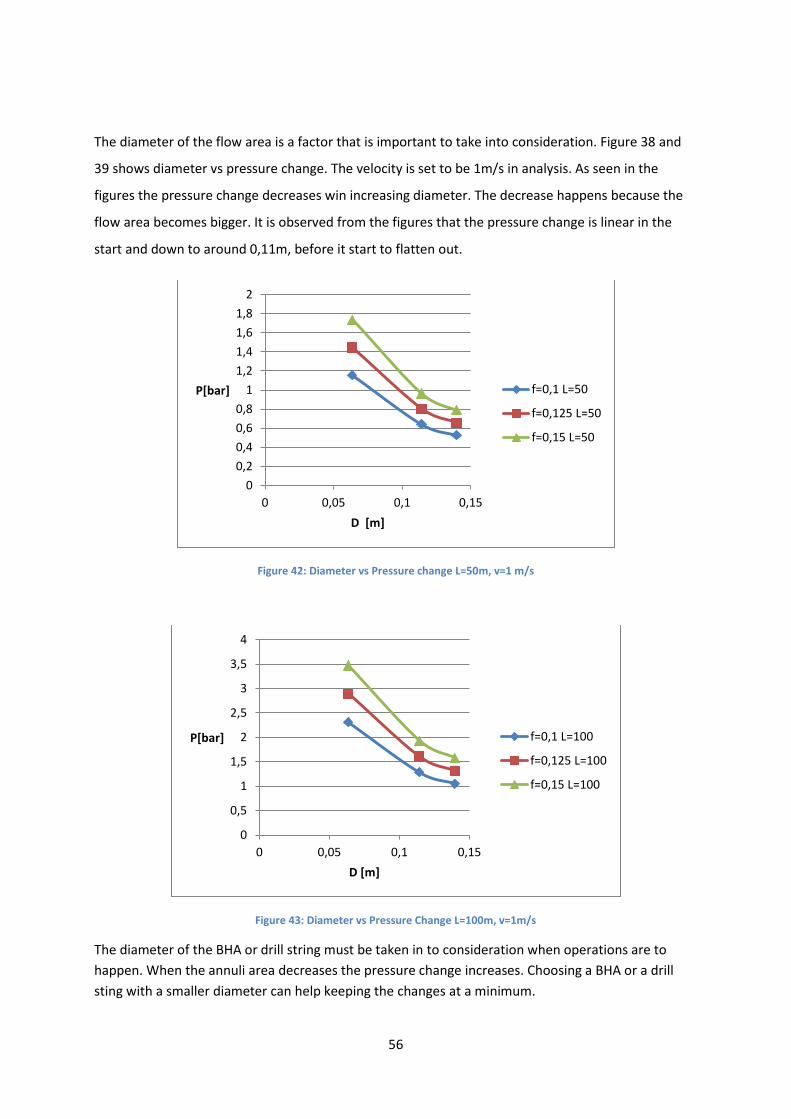
The diameter of the flow area is a factor that is important to take into consideration. Figure 38 and

39 shows diameter vs pressure change. The velocity is set to be 1m/s in analysis. As seen in the

figures the pressure change decreases win increasing diameter. The decrease happens because the

flow area becomes bigger. It is observed from the figures that the pressure change is linear in the

start and down to around 0,11m, before it start to flatten out.

Figure 42: Diameter vs Pressure change L=50m, v=1 m/s

Figure 43: Diameter vs Pressure Change L=100m, v=1m/s

The diameter of the BHA or drill string must be taken in to consideration when operations are to

happen. When the annuli area decreases the pressure change increases. Choosing a BHA or a drill

sting with a smaller diameter can help keeping the changes at a minimum.

0

0,2

0,4

0,6

0,8

1

1,2

1,4

1,6

1,8

2

0 0,05 0,1 0,15

P[bar]

D [m]

f=0,1 L=50

f=0,125 L=50

f=0,15 L=50

0

0,5

1

1,5

2

2,5

3

3,5

4

0 0,05 0,1 0,15

P[bar]

D [m]

f=0,1 L=100

f=0,125 L=100

f=0,15 L=100

57

7. Discussion

The model published by Brooks in 1982 is discussed and adjusted in chapter 3.1 has been tested in

EXCEL and MATLABT. The objective of this project was to improve the knowledge of surge and swab

pressures and build a model that calculates these. The results presented in chapter 6 shows that this

has been achieved. Brook’s model have been further adjusted and translated into a MATLAB script

and an Excel program that calculates the pressure drop. The MATLAB script can be found in Appendix

C. The model shows good result in laminar flow, The model also shows that the surge and swab

pressures increases rapidly when the power law index K is low and when the flow behavior index n is

below 0,5. The model shows that as the diameter of the BHA increases the area of the annulus

decreases and the pressure drop increases.

Pressure change in turbulent flow has given good and realistic results. The model used in this thesis

gives good an indication on the what pressure changes that can be expected. The results show that

the pressure changes linearly when changing the length and exponentially when increasing the

velocity. The pressure change decreases with increasing diameter.

7.1 Quality of model

The model gives good and realistic results under laminar and turbulent flow conditions. It is easy to

change parameters to check results with for example other diameters on the piping, or change the

tripping speed to find what needs to be done not to get a to high pressure change.

The shortcoming of the model is that it has not been properly tested properly. Since it has been

difficult to get drilling data from the industry, the testing of the model has been done with fictive

data with a basis of some data from the drilling report. However, the data tested with are realistic

values that should be in good comparison with the data used in real operations.

7.2 Quality of data

Unfortunately, the model was not tested up against real time drilling data. All companies approached

have confidential drilling reports, and were not willing to share. The drilling report provided was a

confidential internal document that could be used to get realistic values for the sensitivity analysis.

58

7.3 Future work

For future work it would be of interest to test the model with real drilling data, this to ensure that

the results are good and within what is realistic. Companies need to provide drilling data from

historical wells.It is easier to see what parameters affect the results when more tests have been

made available.

The cling factor is a factor that we know little about, and it would be interesting to get a better

understanding of this area. A closer study of the clinging of mud to the drill string can be of great

importance, especially in future narrow wells.

To make the program more professional the program can be transformed from the EXCEL document

it now is, into user friendly software.

59

8. Conclusion

Based on the results and evaluations the conclusions about Surge and swab pressure changes are as

follows:

In laminar flow the velocity of drilling operations as tripping or running the drill string is of

great importance to the pressure change. Pressure change is dependent on the diameter and

length of Bottom Hole Assembly or Drill string The larger the BHA diameter or drill string, the

higher the pressure change gets. R-Rds -> 0 then ΔP -> ∞

When the Flow Behavior Index n gets smaller than 0,5 a rapid increase in pressure change

occurs. Decreasing Power Law Constant K gives an increasing pressure change.

In turbulent flow the velocity of the drill string and the mud is of great importance for

calculating the pressure change. The pressure change increases exponentially with increased

velocity. The length of the section gives a linear change in pressure, and the pressure change

is also depended on the annular space. Increased fanning friction factor leads to ha higher

pressure.

To reduce the pressure changes it is important to manage the velocity and the diameter of

the drill sting or BHA.

The model is a useful tool to calculate pressure change and equivalent circulating density in a

well. Both laminar- and turbulent flow models gives realistic results. However, the model is

compared and tested towards real time drilling data.

The model needs to be tested and compared with real time drilling data.

The cling factor should be studied, and be included in the program if possible. The effects of

the cling factor may change the results.

60

Nomenclature

Parameters

a Constant A Area b constant C1 Constant C2 Constant D Diameter f Friction F Fanning friction factor Inclination K Power Law Constant Cling Constant L Length n Flow Behavior Index P Pressure Q Flow R Radius Rc Radius Cling Rds Radius of drill string Rwell- Radius of wellbore v Velocity V Volume Shear Rate µ Viscosity Share rate Density

61

Abbreviations

BHA Bottom Hole Assembly ECD Equivalent Circulating Density He Total vertical elevation Hf Frictional head NAF Non Aqueous Fluids NOV National Oilwell Varco OMD Oil Based Mud Re Reynolds number RPM Rotations Per Minute TH Total Head WBM Water Based Mud

62

Reference list:

Brooks, A.G. (1982). Swab and Surge Pressures in Non-Newtonian Fluids. Exploration Logging Inc.

Burkhardt, J. A. (1961). Wellbore pressure surges produced by pipe movement. Journal of petroleum

technology, 13 (6), 595-605.

Bourgoyne, A. T., Millheim, K. K., Chenevert, M. E., & Young, F. S. (1986).Applied drilling engineering

(2nd ed.; J. F. Evers & D. S. Pye, Eds.). Society of Petroleum Engineers.

Adebayo and Chinonyere (2012). Sawdust As A Filtration Control And Density Additives in Water

Based Drilling Mud. International Journal of Scientific & Engineering Research

Schubert, J.(2010). Well Controll , Society of Petroleum Engineers.

Cannon, G. E. (1934). Changes in hydrostatic pressure during withdrawing of drillpipe from the hole. In Presented at spring meeting. Southwestern district. fort worth. Texas. April 1034. (Vol. 1, p. 7). Mitchell, R. F. (1988, September). Dynamic surge/swab pressure predictions. SPE Drilling engineering, 3 (3), 325-333. Mitchell, R. F. (2004). Surge pressures in low-clearance liners. In Iadc/spe drilling conference, 2-4 march 2004, Dallas, Texas (p. 9). Society of Petroleum Engineers. (Document ID87181-MS)

Gjerstad, Time, BjørkVoll. (2013). A Medium-Order Flow Model for Dynamic Pressure Surges in

Tripping Operations. Society of Petroleum Engineers

R. Srivastav, F. C. R. A. A. S., M. En_s. (2012). Surge and swab pressures in horizontal and inclined wells. In Spe latin america and Caribbean petroleum engineering conference, 16-18 april 2012, mexico city, Mexico (Vol. 1, p. 8). Crespo, Ahmed, Enfis, Saasen, Amani (2012). Surge and Swab Pressure Predictions for Yield-Power-Law Drilling Fluids. Seciety of Petroleum Engineers Skalle, P. (2012). Drilling fluid engineering. Ventus publishing Aps. Oil, S., & gas dictionary. Retrieved from http://www.glossary.oilfield.slb.com Naley.H (2012). Swab pressures determined experimentally and theoretically

Haliburton. (2012). Lost circulation Retrieved from

:http://www.halliburton.com/public/cem/contents/Overview/images/flexplug.gif

63

Celtiqueenergie (2014) Retrieved from: [http://www.celtiqueenergie.com/Uploads/Geological-

Survey-Frac-v3-3Z1334156142.jpg]

Nial Barker(2010) Retrieved from

http://blog.nialbarker.com/wpcontent/uploads/2010/03/laminar_turbulent_flow.gif

Enigineeringtoolbox (2014) Retrieved from: http://www.engineeringtoolbox.com/laminar-

transitional-turbulent-flow-d_577.html

ODP(2010) Retrieved from:

[http://www-odp.tamu.edu/publications/tnotes/tn31/ris/images/ris_1.jpg, EditedAndreas Grav

Karlsen]

Aliimg (2010) Retrieved from: http://i01.i.aliimg.com/photo/v0/108779901/Mud_Balance.jpg

Survey (2005). Retrieved from http://people.sju.edu/~phabdas/physics/viscosity2.gif

Solutions(2014). Retrieved from

http://solutions.3m.com/3MContentRetrievalAPI/BlobServlet?lmd=1342614075000&locale=en_WW

&assetType=MMM_Image&assetId=1319233768969&blobAttribute=ImageFile

Airdrilling (2012). Retrieved from: http://www.airdrilling.com/images/underbalanced-drilling.jpg

64

Appendix A

Appendix A gives an overview of how the different calculations and inputs are set up in the EXCEL

calculator. Pictures from the program with a short description are added.

Description of program:

The main sheet is the sheet that needs input filled in. Information from the different well sections are

to be inserted and the values desired to be calculated will be shown in the “Output” side of the

sheet. The user can decide what information they want, and what sections of the well they want to

take a closer look at. All the calculations are done in linked sheets that you can see beneath.

65

Main Sheet , EXCEL Program

66

This sheet calculates if the flow is laminar or turbulent. Further on the pressure loss is chosen from

the two different calculations depending on the condition of the flow. All cells are in this sheet linked

together so if you are to change one of them the rest will follow.

Pressure loss Sheet

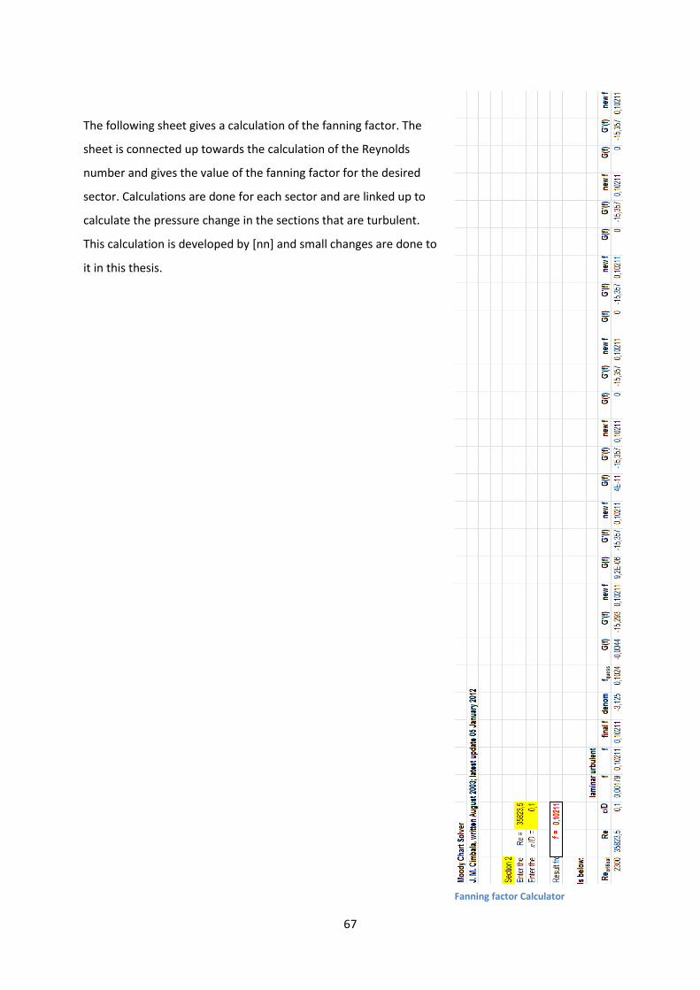
67

The following sheet gives a calculation of the fanning factor. The

sheet is connected up towards the calculation of the Reynolds

number and gives the value of the fanning factor for the desired

sector. Calculations are done for each sector and are linked up to

calculate the pressure change in the sections that are turbulent.

This calculation is developed by [nn] and small changes are done to

it in this thesis.

Fanning factor Calculator

68

The ECD calculations are in a separate sheet.

Calculations for the ECD are done for each

section. The calculations are based on the

work of associate professor Pål Skalle. The

pressure change due to rotation and

acceleration are in this thesis neglected, due

to the complexity of this.

ECD Calculations

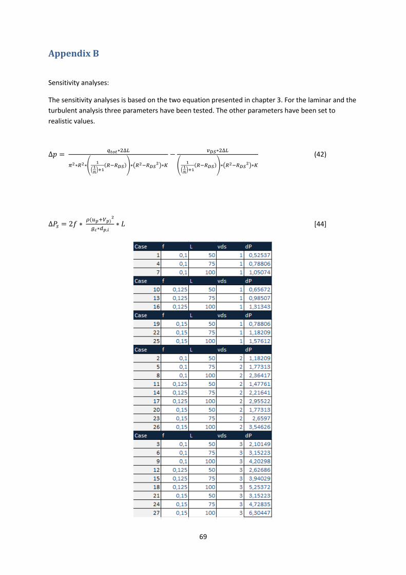
69

Appendix B

Sensitivity analyses:

The sensitivity analyses is based on the two equation presented in chapter 3. For the laminar and the

turbulent analysis three parameters have been tested. The other parameters have been set to

realistic values.

(

(

) ( )) (

)

(

(

) ( )) (

)

(42)

( )

[44]

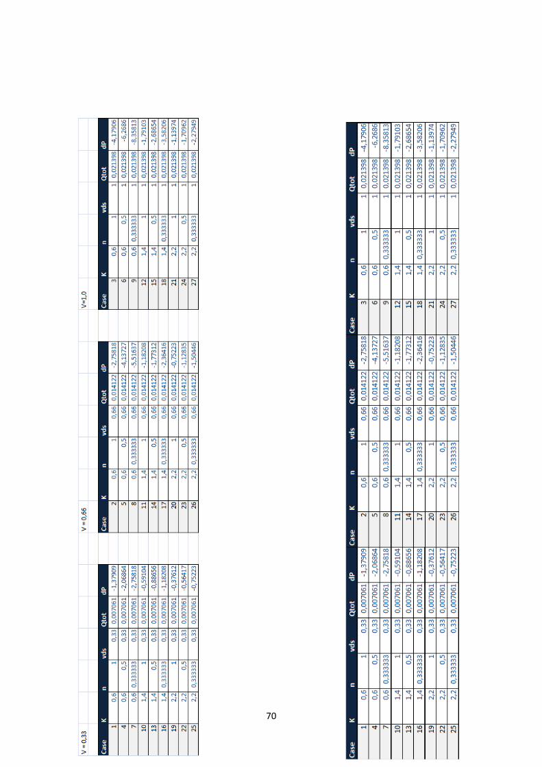
70

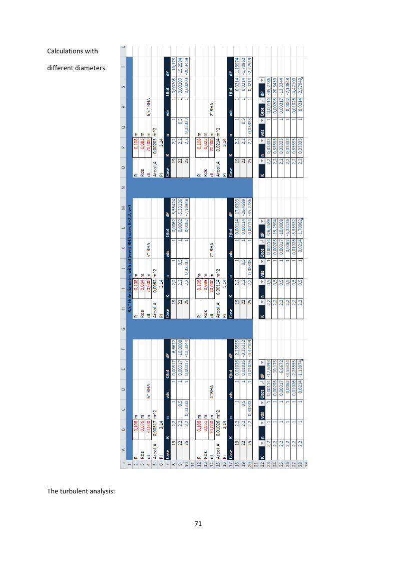
71

Calculations with

different diameters.

The turbulent analysis:

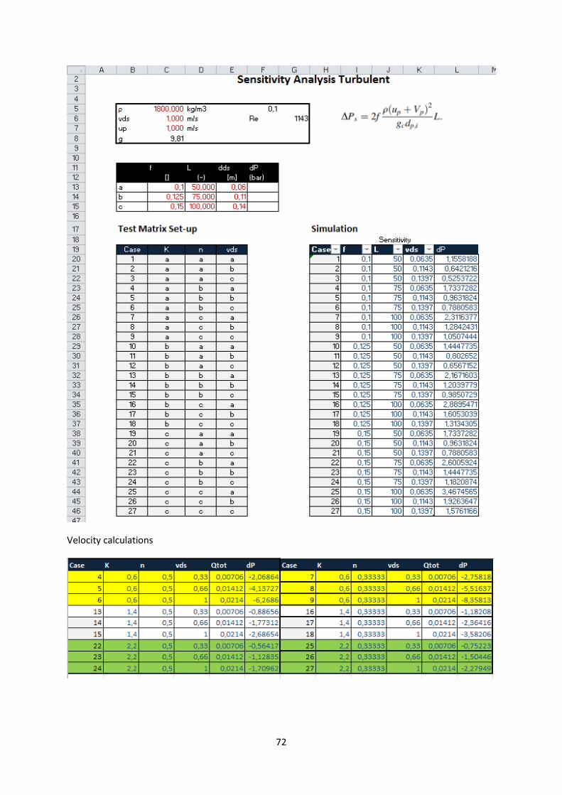
72

Velocity calculations

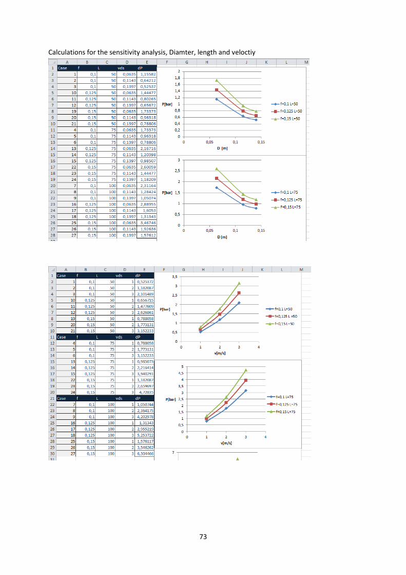
73

Calculations for the sensitivity analysis, Diamter, length and veloctiy

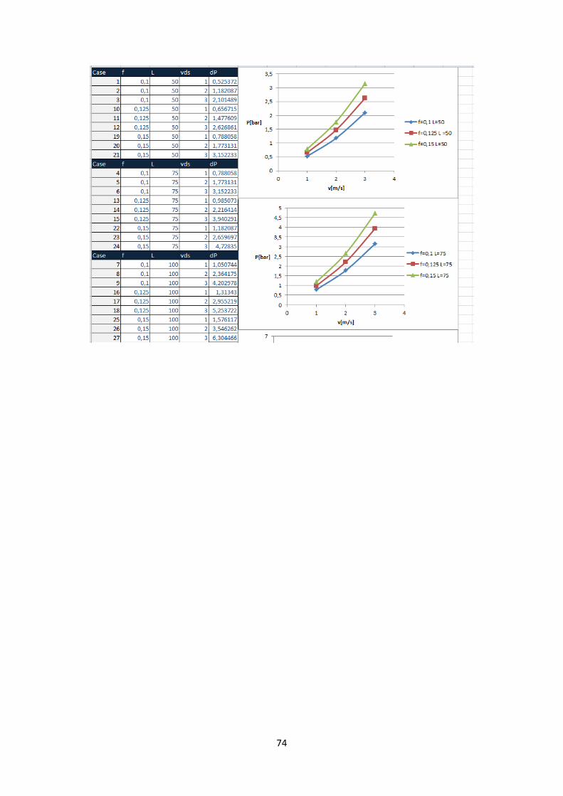
74

75

Appendix C

MATLAB script to calculate laminar flow conditions.

%MATLAB Program on 5 steps to cling and Surge And Swab

%Use Paal Skalle’s model from ”Boreslam” kompedium

%Decleration of various parameters

rho=1200; %kg/m3 – the density of the mud

rho2=1350; %kg/m3 – the density of new mud

rhowater=1000; %kg/m3 – the 75nside75 of sea water

vds1=1.0; %m/s – velocity of drill string while tripping

vds2=1.5; %m/s

vds3=2.0; %m/s

vmud=5; %m/s – velocity of drilling fluid

R=0.108; %m – Radius of well

Rds=0.07; %meter – radius of drill string

Rc=0.01; %Radius of drill string +cling

R0=0.09; %Radius to max velocity

Pi=0; %mPa – The 75nside pressure of drill pipe

Pann=0; %mPa – The pressure in the annulus

Pform=250*10^5; %mPa – The pressure of the formation

TVD=2000; %Total Vertical Depth

dwater=[1:200]; %meter – Depth of sea water

g=9.81; %m/s^2 – Gravitation

tau=0; %Forces ( need to be looked at )

DeltaP=0; %mPa

DeltaL=70; %meter – Length of Bottom hole assembley

qtot=100; %m^3/s Total Bulk flow

qpump=0; %m^3/s Total pump flow

qDS=0; %m^3/s Flow in Drill String

K=0.20; % Need numbers

n=1; % n goes from 1 to 0,333

n2=0,5 ;

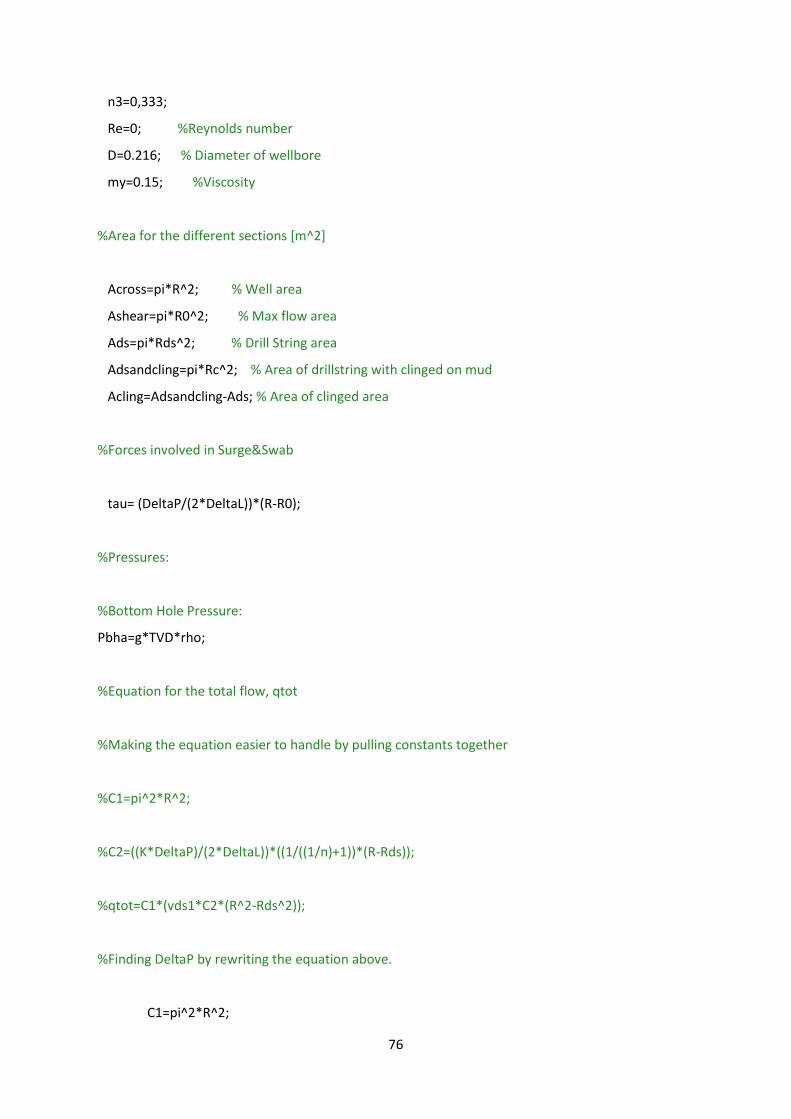
76

n3=0,333;

Re=0; %Reynolds number

D=0.216; % Diameter of wellbore

my=0.15; %Viscosity

%Area for the different sections [m^2]

Across=pi*R^2; % Well area

Ashear=pi*R0^2; % Max flow area

Ads=pi*Rds^2; % Drill String area

Adsandcling=pi*Rc^2; % Area of drillstring with clinged on mud

Acling=Adsandcling-Ads; % Area of clinged area

%Forces involved in Surge&Swab

tau= (DeltaP/(2*DeltaL))*(R-R0);

%Pressures:

%Bottom Hole Pressure:

Pbha=g*TVD*rho;

%Equation for the total flow, qtot

%Making the equation easier to handle by pulling constants together

%C1=pi^2*R^2;

%C2=((K*DeltaP)/(2*DeltaL))*((1/((1/n)+1))*(R-Rds));

%qtot=C1*(vds1*C2*(R^2-Rds^2));

%Finding DeltaP by rewriting the equation above.

C1=pi^2*R^2;

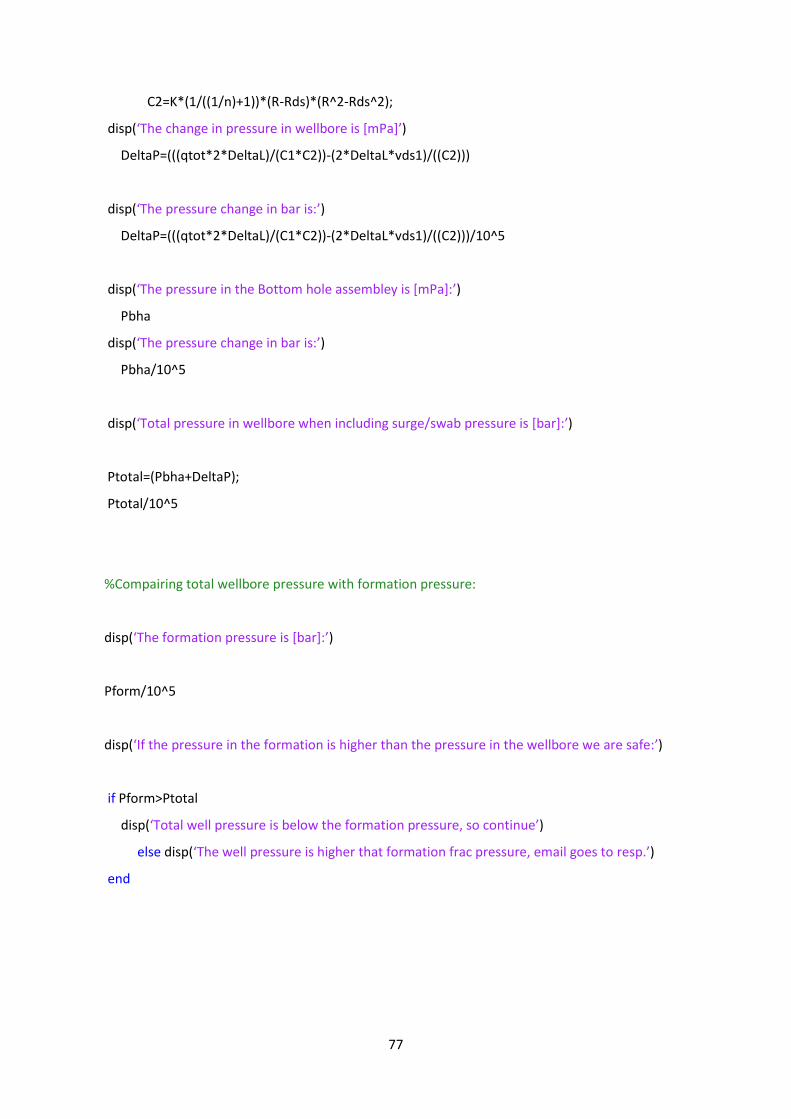
77

C2=K*(1/((1/n)+1))*(R-Rds)*(R^2-Rds^2);

disp(‘The change in pressure in wellbore is [mPa]’)

DeltaP=(((qtot*2*DeltaL)/(C1*C2))-(2*DeltaL*vds1)/((C2)))

disp(‘The pressure change in bar is:’)

DeltaP=(((qtot*2*DeltaL)/(C1*C2))-(2*DeltaL*vds1)/((C2)))/10^5

disp(‘The pressure in the Bottom hole assembley is [mPa]:’)

Pbha

disp(‘The pressure change in bar is:’)

Pbha/10^5

disp(‘Total pressure in wellbore when including surge/swab pressure is [bar]:’)

Ptotal=(Pbha+DeltaP);

Ptotal/10^5

%Compairing total wellbore pressure with formation pressure:

disp(‘The formation pressure is [bar]:’)

Pform/10^5

disp(‘If the pressure in the formation is higher than the pressure in the wellbore we are safe:’)

if Pform>Ptotal

disp(‘Total well pressure is below the formation pressure, so continue’)

else disp(‘The well pressure is higher that formation frac pressure, email goes to resp.’)

end

78

Re=rho*vmud*D/my;

disp(‘The Reynoldsnumber is:’)

Re

if Re<1800

disp(‘The flow is laminar’)

else disp(‘The flow is turbulent’)

end