SURFACE WATER PATHWAY - DEUkisi.deu.edu.tr/orhan.gunduz/turkce/diger/8_SW_Pollution.pdf ·...
183
7_Surface Water Pollution SURFACE WATER PATHWAY Mustafa M. Aral MESL @CEE,GT http://mesl.ce.gatech.edu/ [email protected]
Transcript of SURFACE WATER PATHWAY - DEUkisi.deu.edu.tr/orhan.gunduz/turkce/diger/8_SW_Pollution.pdf ·...

7_Surface Water Pollution
SURFACE WATER PATHWAY
Mustafa M. Aral
MESL @CEE,GThttp://mesl.ce.gatech.edu/[email protected]

7_Surface Water Pollution
Surface Water Regulations
For centuries, fecal waste and other pollutants were dumped in rivers, with “dilution is considered to be the solution to pollution.”
In the mid-twentieth century, many rivers in USA and streams were open sewers, choking on everything from human waste to highly toxic industrial discharges.

7_Surface Water Pollution
Surface Water Regulations: 1
� Public Health Service Act of 1912
� U.S. first water-quality standards created

7_Surface Water Pollution
Surface Water Regulations:
� Clean Water Act (CWA) of 1972� Jurisdiction over water quality in rivers,
lakes, estuaries, and wetlands
� Regulations for wastewater effluents
� Goals of “fishable and swimmable” waters throughout the U.S, by 1983
� By late-1990s, 40 percent of surface water in U.S. not suitable for fishing, swimming, or other designated uses
7_Surface Water Pollution
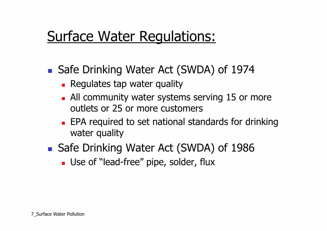
� Safe Drinking Water Act (SWDA) of 1974
� Regulates tap water quality
� All community water systems serving 15 or more outlets or 25 or more customers
� EPA required to set national standards for drinking water quality
� Safe Drinking Water Act (SWDA) of 1986
� Use of “lead-free” pipe, solder, flux
Surface Water Regulations:

7_Surface Water Pollution
Surface Water Regulations:
� National Pollutant Discharge Elimination System (NPDES)
� Permit issued under Clean Water Act
� Requires discharger to meet certain technology-based effluent limits and perform effluent monitoring

7_Surface Water Pollution
� 1990s: Water Quality Inventory found almost 40 percent of U.S. rivers and 45 percent of lakes are polluted.
� More than 95 percent of water tested near four population centers in Great Lakes between 2001 and 2002 contained unsafe levels of mercury and pesticides according to a National Wildlife Federation report.

7_Surface Water Pollution

7_Surface Water Pollution

7_Surface Water Pollution
Since late 1970s
� Billions of dollars have been invested since 1972 building and upgrading sewage treatment facilities.
� Nationally, more than thirty thousand major industrial dischargers pre-treat their wastewater before it enters local sewers.
� By 2000, some 75 percent of toxic discharges, including heavy metals and PCBs, were being prevented.

7_Surface Water Pollution
Drinking-Water Standards
� Primary Standards� Specify Maximum Contaminant Levels (MCLs) based on
health-related criteria
� Secondary Standards� Unenforceable guidelines based on aesthetics (taste, odor,
color) and non-aesthetics (corrosivity, hardness)
� Maximum Contaminant Level Goals (MCLGs)� Unenforceable goals set at levels that present no known or
anticipated health effects, regardless of technological feasibility or cost

7_Surface Water Pollution
Open Channels Review
Characterized by flows with a free surface:a. Simplification � P = 0 at the surfaceb. Complication � Free surface configuration is not known
Datumz1
y1Pz
γ+
2
1
2
V
g
oS
1
EL
2
2
2
V
g
y2
z2
Lh
HGL

7_Surface Water Pollution
FLOW CLASSIFICATIONS
Laminar FlowTurbulent Flow
Uniform FlowVaried Flow
Gradually varied FlowRapidly Varied Flow
Sub-Critical FlowSuper-Critical Flow
µ
ε
→
→
,y P→
,V c→

7_Surface Water Pollution
GVFRVF GVF Uniform GVF GVFRVF
Uniform Flow: Weight Forces are balanced with shear forces, pressure distribution is hydrostatic,
depth is constant, EL� HGL� Channel slope parallel
c
v
ypFFp

7_Surface Water Pollution
UNIFORM FLOW EQUATIONS:
1F
2F
W
ny
wFτ
sinW θ
θ
1 2
0F M a
F F
= =
=
∑�� �
sin
sin
w w
Lo
F PL
W AL
hS
L
τ τ
γ θ
θ
=
=
= =
L
ny
AP

7_Surface Water Pollution
1 2sin 0
sin
w
Lw o h o h
F W F PL
AL A hS R S R
PL P L
θ τ
γ θτ γ γ γ
+ − − =
= = = =
( )
( ) ( )
2
2
2
1/ 2
1/ 2 1/ 2
8
8
8 8
8
w
Lw h
Lh h o
h o
fV
f V hR
L
g h gV R R S
f L f
gV R S
f
τ
ρ
ρτ γ
=
= =
= =
=
1F
2F
W
ny
wFτ
sinW θ
θ
L
( ) ( )
1/ 2
1/ 2 1/ 2
8Chezy constant
h o
gC
f
V C R S
=
=
( ) ( )
( ) ( )
1/6 1/6
2/3 1/2
2/3 1/2
1.49 1
1.49
1.0
h h
h o
h o
C R or Rn n
V R Sn
V R Sn
= = =
=
=
BU
SI
Mannings eqn

7_Surface Water Pollution

7_Surface Water Pollution
Hydraulic Radius Plays an important role in open channel computations:hR
2h
A ByR
P y B= =
+B
y
Constant B � Deep Channels
0 0
2
h
h
y R
By R
= =
→ ∞ =22
h
B BR
y B
y y
= =
+
y
hR
2
B

7_Surface Water Pollution
Hydraulic Radius Plays an important role in open channel computations:hR
2h
A ByR
P y B= =
+B
y
Constant Depth y � Wide Channels
0 0h
h
B R
B R y
= =
→ ∞ = 2h
yR y
y B
B B
= =
+
B
hR
y

7_Surface Water Pollution
Shear Velocity:*
u
L
V
wτ
*u
*u
*u
*uB
yz
V(z)
y*
u
max Largest eddy sized y=

7_Surface Water Pollution
The eddies cause vertical / lateral or longitudinal diffusion which proceed at a rate given by vertical/lateral diffusivity proportional to the product of the orbital velocity u* and the maximum length scale of an eddy
*
verticalD u y=
But what is u*?
L
V
wτ
*u
*u
*u
*uB
yMass Acceleration Force× =
*
w
uLBy LBρ τ
τ× =
*
yeddy turn around time
uτ ≈ −
( )2
*
wuρ τ=

7_Surface Water Pollution
L
V
wτ
*u
*u
*u
*uB
y
( )2
*
wuρ τ=
* wu friction velocityτ
ρ=
Lw h o h
hR S R
Lτ γ γ= =
* h oh o
R Su gR S
γ
ρ= =

7_Surface Water Pollution
2
-9 2
2
9
(units)
Molecular diffusion coefficient of salt (NaCL) = 1.5x10 m /s
Given a cup of depth 5cm how long will it take
for diffusive concentration to reach the top of the cup:
0.0519.29
1.5 10
LD
t
t dayx
−
=
= = s
DEFINITION OF DIFFUSION COEFFICIENT:
This is not going to be useful for environmental dilution

7_Surface Water Pollution
VERTICAL DIFFUSION:
( )*
verticalD f u y=
*0.067 0.067vertical h o
D u y y gR S= =
Empirical constant � 0.067 ~ 0.05 – 0.07
Remember the mechanical mixing molecular mixing concept in GW applications
Mechanical mixing component due to turbulence
0.1H p m p m
D V D LV Dα= + = +

7_Surface Water Pollution
For a contaminant discharge at mid depth
*0.067vertical
D u y=
( )
2
**
*
1
0.2684 0.067
3.73
v
v
y y
uu y
y
u
τ
τ
= =
=
*3.73
v v
yx V V
uτ= =
xv
VERTICAL DIFFUSION:
y/2
z
x
2
1
v
y
τ=
2
4 v
y
τ=

7_Surface Water Pollution
For a contaminant discharge at the base
*0.067vertical
D u y=
( )
2
**
*
1
0.0670.067
14.9
v
v
y y
uu y
y
u
τ
τ
= =
=
*14.9
v v
yx V V
uτ= =
VERTICAL DIFFUSION:
xv
y
z
x
2
v
y
τ=

7_Surface Water Pollution
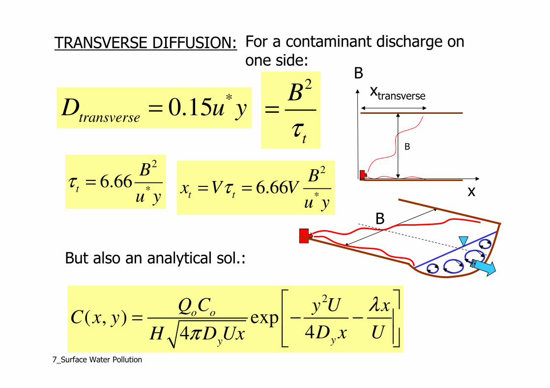
TRANSVERSE DIFFUSION:
( )*
transverseD f u y=
*0.15 0.15transverse h o
D u y y gR S= =
Empirical � 0.15 ~ 0.1 – 0.4
For a contaminant discharge on one side:
B
Width
x
xtransverse
Plan view

7_Surface Water Pollution
TRANSVERSE DIFFUSION: For a contaminant discharge on one side:
*0.15transverseD u y=
2
*6.66
t
B
u yτ =
2
*6.66t t
Bx V V
u yτ= =
B
B
x
xtransverse
B
2
t
B
τ=

7_Surface Water Pollution
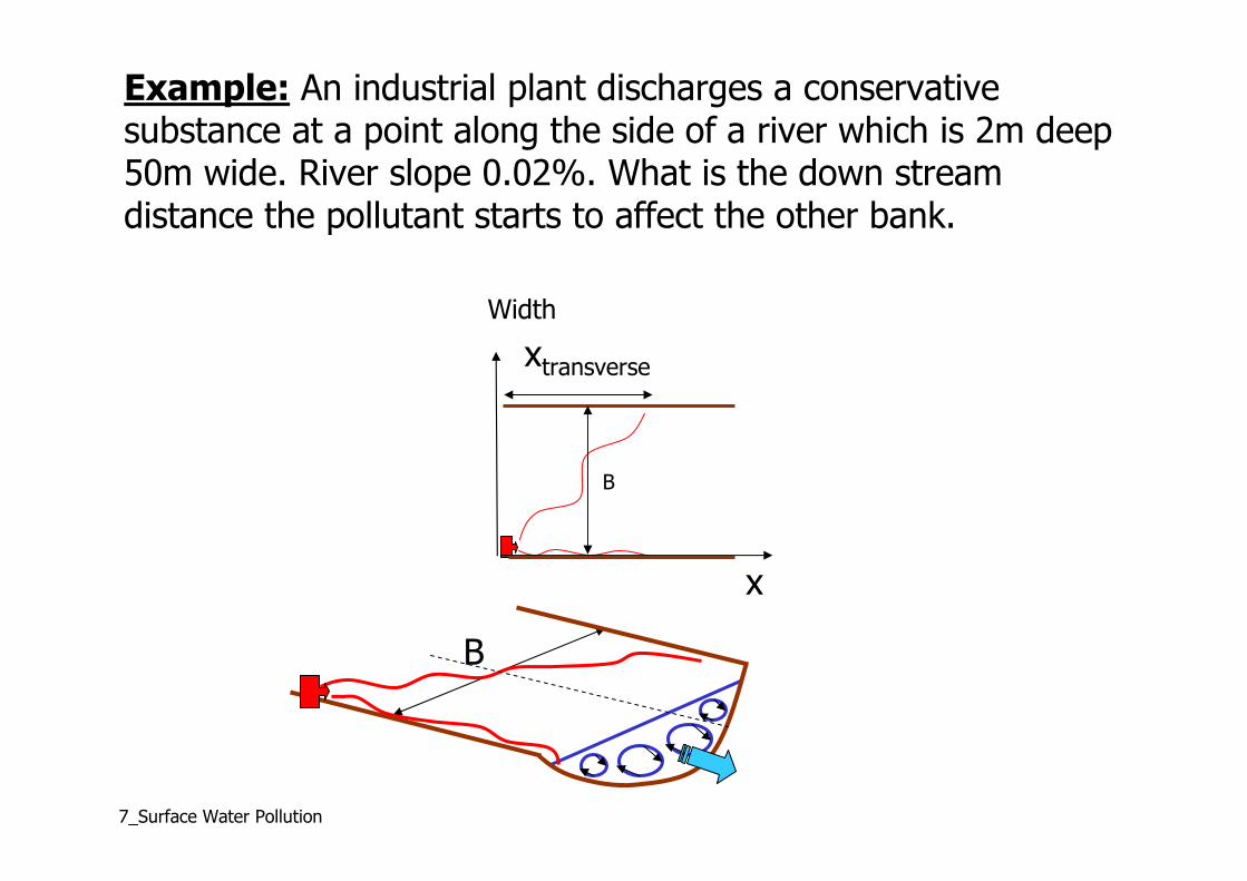
Example: An industrial plant discharges a conservative substance at a point along the side of a river which is 2m deep 500m wide. River slope 0.02%. What is the down stream distance the pollutant starts to affect the other bank.
B
Width
x
xtransverse
B

7_Surface Water Pollution
for annings n 0.035 0.61 /M V m s= =
( ) ( ) ( )* 49.81 1.85 2 10 0.06 /h ou gR S m s−= = × =
2 501.85
2 50 2h
AR m
P
×= = =
+ +
Example: An industrial plant discharges a conservative substanceat a point along the side of a river which is 2m deep 50m wide.River slope 0.02%. What is the down stream distance the pollutant starts to affect the other bank.
( ) ( )2 / 3 1/ 21.0
h oV R Sn
=
( ) ( )* 20.15 0.15 0.06 2 0.018 /transverse
D u y m s= = =
( )
2 2
*
506.66 6.66 138750 38.54 1.6
2 0.06t
Bs days days
u yτ = = = = =
( )138750 0.61 / 84637.5 84.6transverse
x s m s m km= = =
B
B
x
xtransverse
B

7_Surface Water Pollution
LONGITUDINAL DIFFUSION:
( )*
longitudinalD f u y=
*5.93 5.93longitudinal h o
D u y y gR S= =
Shallow and wide rivers
Deep and narrow rivers where bank shear is important
2 2
*0.011longitudinal
V BD
u y=
Actually there is more…

7_Surface Water Pollution
SUMMARY:
( ) ( )
( ) ( )
2 / 3 1/ 2
2 / 3 1/ 2
1.49
1.0
h o
h o
V R Sn
V R Sn
=
=
Mannings Eqn:
( )*D f u y=
*
h ou gR S=
*
yeddy turn around time
uτ ≈ −
h
AR
P=
ny
AP

7_Surface Water Pollution
*0.067vertical
D u y=
*0.15transverseD u y=
*5.93longitudinalD u y=
* h oh o
R Su gR S
γ
ρ= =y = flow depth
Empirical � 0.15 ~ 0.1 – 0.4
Empirical � 0.067 ~ 0.05 – 0.07
2 2
*0.011longitudinal
V BD
u y=
Shallow and wide rivers Deep and narrow rivers where bank shear is important
SUMMARY:

7_Surface Water Pollution
*
*
0.152
0.067
transverse
vertical
D u y
D u y= ≈
*
*
5.9390
0.067
longitudinal
vertical
D u y
D u y= ≈
*
*
5.9340
0.15
longitudinal
transverse
D u y
D u y= ≈
SUMMARY:
0.01vertical longitudinal
D D=
0.025transverse longitudinalD D=

7_Surface Water Pollution
Stages of Model Complexity:
1.CSTR models
2.Turbulent Mixing analysis
3.Plug flow models (no Turbulent Mixing)
4.Empirical Models: Near Field, Far Field Mixing models.
5.Advection + diffusion models (Conservation of Mass).
6.Advection + diffusion + reaction models (Conservation of Mass).

7_Surface Water Pollution
Mass balance models based on a PLUG-FLOW SYSTEM: (no Turb. diffusion)
ReactionsAccumulation Inputs Outputs= − ±
ny
θ
QC ( )Q C C+ ∆
x∆
d V( )( )
CQC Q C C RV
dt= − + ∆ ±
Constant flowsConstant x-section area A
V A x= ∆
( )Q C CdC QCR
dt A x A x
+ ∆= − ±
∆ ∆
( ) ( )Q C Q CdC QCR
dt A x A x A x
∆= − − ±
∆ ∆ ∆

7_Surface Water Pollution
ny
θ
QC ( )Q C C+ ∆
x∆
( ) ( )Q C Q CdC QCR
dt A x A x A x
∆= − − ±
∆ ∆ ∆
( )Q CC CR V R
t A x x
C CV R
t x
∆∂ ∂= − ± = − ±
∂ ∆ ∂
∂ ∂+ = ±
∂ ∂Time dependent
CV R
x
∂= ±
∂Steady state

7_Surface Water Pollution
CV R
x
∂= ±
∂Steady state
if reaction is first order decay dC R k
C R kCdx V V
= ± = − = −
0
0
ln
o
o
C x
C
xC
C
dC kdx
C V
dC kdx
C V
kxC
V
= −
= −
= −
∫ ∫( )
ln
exp /
o
o
C kx
C V
C C kx V
−=
= −

7_Surface Water Pollution
Variable flows and Variable x-section area A
( )
( )
exp
exp
o
o
Q Q qx
A A ax
=
=,
o oA Q
d V( )( )
CQC Q C C RV
dt= − + ∆ ±
d V( )( ) ( )
CQC Q Q C C RV
dt= − + ∆ + ∆ ±
Previous model
d VC V
dt+ ( ) ( )
dCQC Q Q C C RV
dt= − + ∆ + ∆ ±
V ( ) ( )dC
QC Q Q C C RVdt
= − + ∆ + ∆ ±
Volume is not changing as a function of time

7_Surface Water Pollution
V ( ) ( )dC
QC Q Q C C RVdt
= − + ∆ + ∆ ±
VdC
QC QC C Q Q C Q C RVdt
= − − ∆ − ∆ − ∆ ∆ ±
dC C Q Q C Q CR
dt A x A x A x
∆ ∆ ∆ ∆= − − − ±
∆ ∆ ∆
C C Q Q C Q CR
t A x A x A x
∂ ∂ ∂ ∂ ∂= − − − ±
∂ ∂ ∂ ∂
Product of two changesAre small relative to other terms
( )1 CQCR
t A x
∂∂= − ±
∂ ∂Q,A and R can be variable
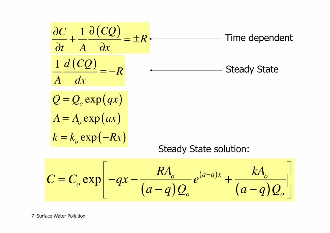
7_Surface Water Pollution
( )1 CQCR
t A x
∂∂+ = ±
∂ ∂Time dependent
Steady State( )1 d CQ
RA dx
= −
( )
( )
( )
exp
exp
exp
o
o
o
Q Q qx
A A ax
k k Rx
=
=
= −
( )( )
( )exp
a q xo oo
o o
RA kAC C qx e
a q Q a q Q
− = − − +
− −
Steady State solution:

7_Surface Water Pollution
2
2
C C CV D kC
t x x
∂ ∂ ∂+ = −
∂ ∂ ∂Time dependent with mixing
We will not discuss the solutions of this differential equation!! May get too complicated.
ACTS uses 1D, 2D and 3D solutions of this model for very complex cases.
Advection and Mixing in rivers (Conservation of Mass based):

7_Surface Water Pollution
LAKES AND RESERVOIRS:
As opposed to rivers: Low advective velocity
Thus they impound water for long time.
An important parameter to consider is the Residency Time (or retention time).
Retention time:
Average time spent for a particle in the lake from inflowto outflow.
r
Volt
Q=
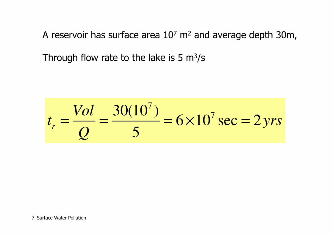
7_Surface Water Pollution
A reservoir has surface area 107 m2 and average depth 30m,
Through flow rate to the lake is 5 m3/s
7730(10 )
6 10 sec 25
r
Volt yrs
Q= = = × =

7_Surface Water Pollution
ReactionsAccumulation Inputs Outputs= − ±
d V( )( )
CQC Q C C RV
dt= − + ∆ ±
Vol.
Q
Lakes:

7_Surface Water Pollution
V ( )C
Q C RVt
∂= − ∆ ±
∂
VC V
t
∂= −
∂( )
r
C kC Vt
−
VC
Vt
∂+
∂
1
r
C k Wt
+ =
Q � volume/time∆C � point concentration
( )W
C tVβ
= ( ) 11 t t
o
r
e C e kt
β β β− − − + = +
Constant W source input over time
Co = background conc.
Vol.
Q

7_Surface Water Pollution
( )W
C tVβ
= ( ) 11 t t
o
r
e C e kt
β β β− − − + = +
If the background concentration is negligible:
( )W
C tVβ
= ( ) 11 t
r
e kt
β β− − = +
Equilibrium concentration t→∞
( )W
C tVβ
= ∞ =1
r
kt
β
= +
If there is backgroundconcentration but no contaminant source input:
1( ) t
o
r
C t C e kt
β β− = = +
What if the contaminant is conservative? k = 0

7_Surface Water Pollution
Dispersion in a lake …… low velocity
2
2
C CD kC
t x
∂ ∂= −
∂ ∂
Again we will not spend time in discussing the solutions to this PDE!! ACTS uses these models and more complex cases.
We will define other models for lakes and reservoirs later.
Q
D=?
*u
( )*D f u y= But there are many other issues.

7_Surface Water Pollution
Empirical Turbulent Mixing Models for Surface Water applications

7_Surface Water Pollution
Mixing Processes and Applications in Surface Waters
� Advective and diffusive transport in water bodies and transport with sediment movement
� Intermedia transfer characterized by adsorption, desorption, precipitation, dissolution, and volatilization
� Degradation and decay
� Chemical transformation which may yield daughter products

7_Surface Water Pollution
Source Conditions:
� Direct discharge from point sources
� Dry and wet deposition from the atmosphere
� Runoff and soil erosion from land surfaces
� Seepage to and from groundwater

7_Surface Water Pollution
Classification of Empirical Models
� Near-field mixing
� Far-field mixing
� Sediment models

7_Surface Water Pollution
H
Near field mixing
2.5 H
Vr
Far Field Mixing
Uo
Diffuser
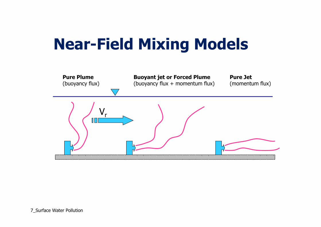
7_Surface Water Pollution
Vr
Pure Plume(buoyancy flux)
Buoyant jet or Forced Plume(buoyancy flux + momentum flux)
Pure Jet(momentum flux)
Near-Field Mixing Models

1_Prerequisites and introduction
ACTS:

1_Prerequisites and introduction
Surface Water:

7_Surface Water Pollution
Near-Field Mixing Models
� Surface point discharges� Stagnant water� Weak cross-currents
� Submerged point discharges� Stagnant water� Weak cross-currents
� Submerged multi-port diffusers� Deep receiving water� Shallow receiving water
7_Surface Water Pollution
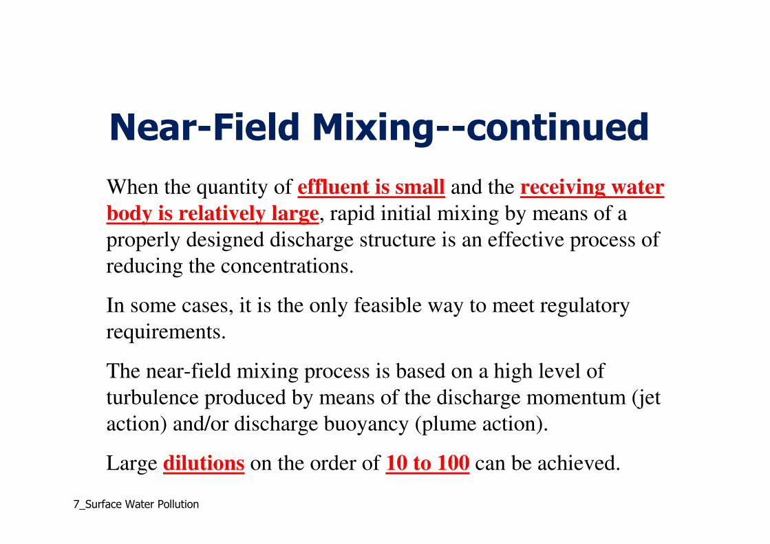
Near-Field Mixing--continued
When the quantity of effluent is small and the receiving water
body is relatively large, rapid initial mixing by means of a
properly designed discharge structure is an effective process of
reducing the concentrations.
In some cases, it is the only feasible way to meet regulatory
requirements.
The near-field mixing process is based on a high level of
turbulence produced by means of the discharge momentum (jet
action) and/or discharge buoyancy (plume action).
Large dilutions on the order of 10 to 100 can be achieved.

7_Surface Water Pollution
Near-Field Mixing
H
hmax
2.5H
hmax to be computed

7_Surface Water Pollution
Characteristic Parameters
Density Deficit
oρρρ −=∆
where: ρo = ambient density, M/L3
ρ = density of discharging fluid, M/L3
∆ρ = density deficit, M/L3

7_Surface Water Pollution
Characteristic Parameters
oo
o
og
UF
�)/( ρρ∆=
Uo = is the (mean) discharge velocity (m/s) (effluent discharge),
ρρρρo = is the ambient density (kg/m3),
∆∆∆∆ρρρρ = is the discharge density deficit (kg/m3),
g = is the acceleration of gravity (m/s),
lo = is a characteristic length scale (m) of the discharge, which is related to its cross-
sectional area Ao by,
� o
oA=
2
Densimetric Froude Number, Fo
7_Surface Water Pollution
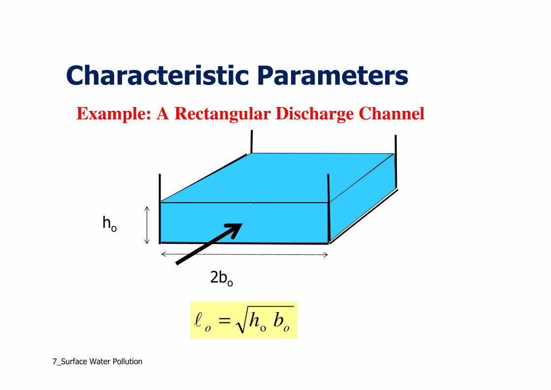
Characteristic Parameters
Example: A Rectangular Discharge Channel
oo bho=�
ho
2bo

7_Surface Water Pollution
Near-Field Mixing--continued
The contaminant concentration is computed by:
S
CC o=
Co is the initial concentration,
S is the dilution, and
C is the concentration at some point of interest, most likely
to be at the end of the near-field mixing zone.

7_Surface Water Pollution
Surface Point Discharges: 1
� Stagnant and Weak Cross-Currents� Deep receiving water
� Stagnant and Weak Cross-Currents� Shallow receiving water
� Strong cross-flow� Shoreline attached jets
� Zero or negative buoyancy

7_Surface Water Pollution
Stagnant and Weak Cross-Currents
Surface Point Discharges: 2
H
hmax
hmax / H > 0.75Shallow Receiving water
hmax / H < 0.75Deep Receiving water
ooFlh 42.0max =
7_Surface Water Pollution
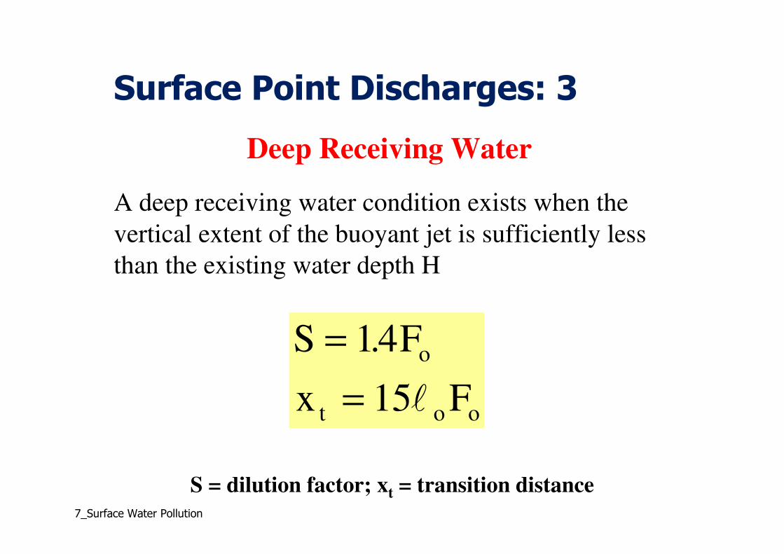
Surface Point Discharges: 3
S F
x F
o
t o o
=
=
14
15
.
�
Deep Receiving Water
A deep receiving water condition exists when the
vertical extent of the buoyant jet is sufficiently less
than the existing water depth H
S = dilution factor; xt = transition distance

7_Surface Water Pollution
Surface Point Discharges: 4
ooFlh 42.0max =
Deep Receiving Water
Maximum vertical penetration of the surface jet:
Occurs at an approximate distance of 5.5loFo from the outfall
H
hmax
5.5loFo

7_Surface Water Pollution
Surface Point Discharges: 5
75.0max >H
h
Shallow Receiving Water
If the bottom of the water body affects the behavior of the
jet, the receiving water can be identified as a shallow water
body. Virtually most river outfalls can be grouped under
this category. A criterion for shallow water conditions
obtained from experimental and field data is:
where H is the depth a the point of maximum plume depth, hmax

7_Surface Water Pollution
Surface Point Discharges: 6
Shallow Receiving Water
An example:
hmax/H = 4/5 = 0.8 > 0.75
H = 5m
hmax = 4mH
hmax

7_Surface Water Pollution
Surface Point Discharges: 7
Shallow Receiving Water
SrS s='
An empirical correction factor, rs can be applied to the
deep-water equations for dilution to account for the
inhibiting effect of a shallow receiving water. Bulk dilution
under shallow water conditions S’ is estimated by:
The empirical factor, rs, is given by:
75.0
max
75.0
=
Hh
rs

7_Surface Water Pollution
Strong Cross Flows
For strong cross flows the plume maybe pinned to the shoreline which restricts mixing. Thus corrections to dilution factor must be implemented.
If:
3/ 2
max0.05
a
R
UR
U
hR
H
−
=
>
Than strong cross flow case should be used:
URUa
Surface Point Discharge: 9
Ua= Cross flow velocityUR = Longitudinal velocity

7_Surface Water Pollution
Strong Cross Flows
'1 1
2 2attached sS S r S= =
For Shallow water:
The extent of near field zone for this case is the smallest of:
2 15oc t o o
x or x FR
= =�
�
Surface Point Discharge: 10

7_Surface Water Pollution
Zero or Negative Buoyancy
All previous models discussed are valid for buoyant discharges. Most jets of effluents are buoyant due to presence of density differences. If the jet does not exhibit density differences (∆ρ→0) than the dilution factor is calculated based on the geometry of the discharge vessel:
0.32x
SD
=
x = downstream distanceD = Diameter of the round discharge point
Surface Point Discharge: 11

7_Surface Water Pollution
Surface Point Discharge: 8
ACTS Interface

7_Surface Water Pollution
Near-Field Mixing Models
� Surface point discharges� Stagnant water� Weak cross-currents
� Submerged point discharges� Stagnant water� Weak cross-currents
� Submerged multi-port diffusers� Deep receiving water� Shallow receiving water

7_Surface Water Pollution
Stagnant Water
Weak Cross-Currents
Surface Point
Discharges
Stagnant Water
Weak Cross-Currents
Submerged Point
Discharges
Deep Receiving Water
Shallow Receiving Water
Submerged Multiport
Discharges
Near Field Mixing Far Field Mixing Sediments
Pathway Models
Surface Water Pathway
Models
ACTS Surface Water Models

7_Surface Water Pollution
Submerged Point Discharges: 1
� Deep receiving water condition
� Buoyant jet rises to the surface and dilution occurs because of turbulent jet entrainment up to surface level
� Shallow receiving water condition
� Discharge momentum is sufficiently strong to cause a dynamic breakdown of the buoyant jet motion and to create a local circulation zone

7_Surface Water Pollution
Submerged Point Discharges: 2
Hz Stratified
Counter FlowDo
Uo
∇∇∇∇
H
z
Bouyant JetDo
Uo
∇∇∇∇Deep discharge with
buoyant jet
Shallow discharge with
circulation

7_Surface Water Pollution
Distinction between deep and shallow water conditions is important.
( / )
oo
o o
UF
gDρ ρ=
∆
0.22o
o
HF
D>
Do diameter of the outfall
Implies deep water condition
Submerged Point Discharges: 3

7_Surface Water Pollution
For deep water conditions buoyant jet models can be used.
5/ 3
2 / 30.11c o
o
zS F
D
− =
z is the distance above the nozzle to the water surfaceSc is the centerline dilution
Dilution at the boundaries of the flow field at z:
1.4 cS S=H
z
Bouyant JetDo
Uo
∇∇∇∇
θ
Submerged Point Discharges: 4

7_Surface Water Pollution
For shallow water conditions:
5/3
2/30.9c o
o
zS F
D
− =
Hz Stratified
Counter FlowDo
Uo
∇∇∇∇
Submerged Point Discharges: 5
Dilution at the boundaries of the flow field at z:
1.4 cS S=

7_Surface Water Pollution
Submerged Point Discharges: 6
ACTS Interface

7_Surface Water Pollution
Near-Field Mixing Models
� Surface point discharges� Stagnant water
� Weak cross-currents
� Submerged point discharges� Stagnant water
� Weak cross-currents
� Submerged multi-port diffusers� Deep receiving water
� Shallow receiving water

7_Surface Water Pollution
Stagnant Water
Weak Cross-Currents
Surface Point
Discharges
Stagnant Water
Weak Cross-Currents
Submerged Point
Discharges
Deep Receiving Water
Shallow Receiving Water
Submerged Multiport
Discharges
Near Field Mixing Far Field Mixing Sediments
Pathway Models
Surface Water Pathway
Models
ACTS Surface Water Models

7_Surface Water Pollution
Multiport diffusers: 1
Typical behavior of wastewater discharged from an ocean outfall
Singh and Hager, 1966, Fig. 3.1

7_Surface Water Pollution
2
4
dB
s
π=
( / )
oo
o
UF
gBρ ρ=
∆
Diffuser details
Singh and Hager, 1966, Fig. 3.2
Multiport diffusers: 2
( )2
4/3 21.84 1 coso o
HF
Bθ> + Deep water condition

7_Surface Water Pollution
2 / 30.27 s
HS F
B
−=
0.58 a D
o
U L HS
Q=
2 / 30.44s
HS F
B
−=Stagnant conditions:
Ambient Cross flow:
Strong Cross flow:
Deep water condition
Multiport diffusers: 3

7_Surface Water Pollution
1/ 22
1 12
2 2
a D a D
o o
U L H U L H HS
Q Q B
= + +
0.67H
SB
=Stagnant conditions:
Ambient Cross flow:
Shallow water condition
Multiport diffusers: 3

7_Surface Water Pollution
Submerged Multiport Diffusers
ACTS Interface

7_Surface Water Pollution
General Classification of Models
� Near-field mixing
� Far-field mixing
� Sediment models

7_Surface Water Pollution
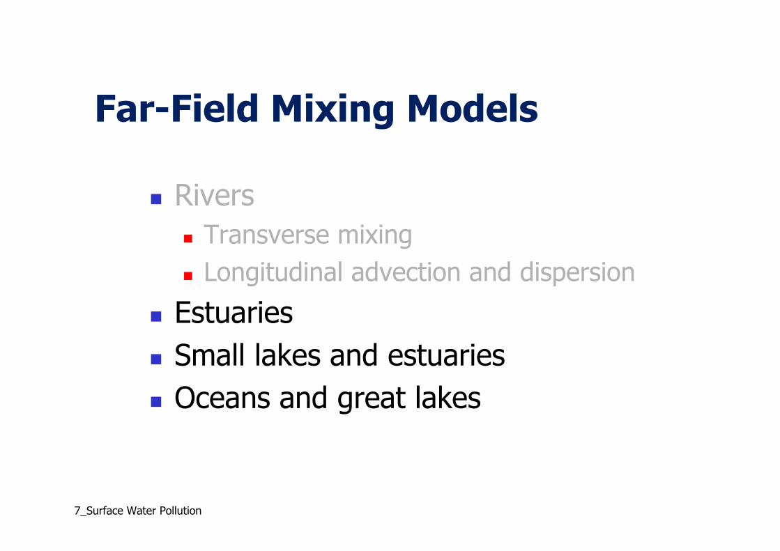
Far-Field Mixing Models
� Rivers
� Transverse mixing
� Longitudinal advection and dispersion
� Estuaries
� Small lakes and estuaries
� Oceans and great lakes

7_Surface Water Pollution
Rivers – Transverse Mixing and
Longitudinal Advection and Dispersion
Near Field Mixing
Transverse Mixing
Longitudinal
Advection and
Dispersion
Rivers Estuaries Small Lakes and
Reservoirs
Oceans and
Great Lakes
Far Field Mixing Sediments
Pathway Models
Surface Water Pathway
Models

7_Surface Water Pollution
Mixing in Rivers
Sewage
A
A
B C
7_Surface Water Pollution
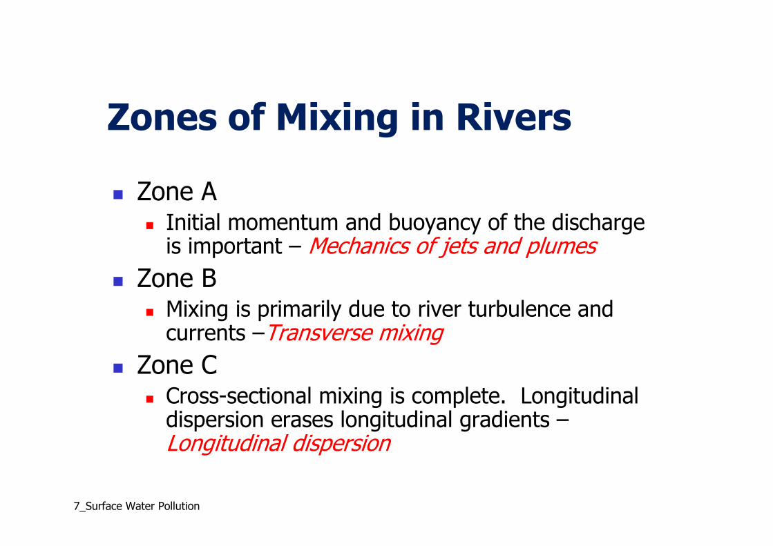
Zones of Mixing in Rivers
� Zone A� Initial momentum and buoyancy of the discharge
is important – Mechanics of jets and plumes
� Zone B� Mixing is primarily due to river turbulence and
currents –Transverse mixing
� Zone C� Cross-sectional mixing is complete. Longitudinal
dispersion erases longitudinal gradients –Longitudinal dispersion

7_Surface Water Pollution
Transverse Mixing in Rivers: 1
x
yC(x,y)
σσσσy
Plume
boundary
U
Point
Source
U
W
C(x,y)
Line source
Line
Source

7_Surface Water Pollution
Transverse Mixing in Rivers: 2
Two-Dimensional Contaminant Concentration
2
( , ) exp44
o o
yy
Q C y U xC x y
D x UH D Ux
λ
π
= − −
Co = initial concentration, M/L2
Qo = initial effluent flow rate, L3/T
x = longitudinal distance, L
y = transverse distance, L
H = depth of river, L
U = ambient river velocity, L/T
λ = radioactive decay (λ = ln2/T1/2), 1/T
Dy= transverse diffusion coefficient, L2/T
Qo and Co may represent variables determined by near-field mixing models
Assuming plume width is much less than river width,

7_Surface Water Pollution
Transverse Mixing in Rivers: 3
2
( , ) exp44
o o
yy
Q C y U xC x y
D x UH D Ux
λ
π
= − −
Interpretation of two-dimensional contaminant
concentration equation
Variation over
width of river
Peak
Concentration

7_Surface Water Pollution
Transverse Mixing in Rivers: 4
2
( , ) exp44
o o
yy
Q C y U xC x y
D x UH D Ux
λ
π
= − −
What is the expression for the concentration of a
conservative substance at any distance downstream of the
source, along the centerline of the river?
0
( , )4
o o
y
Q CC x y
H D Uxπ=
Example
0

7_Surface Water Pollution
Transverse Mixing in Rivers: 5
Two-Dimensional Concentration--continued
*y yD u Hβ=
Dy= transverse diffusion coefficient, L2/T
H = depth of river, L
u* = shear velocity, L/T
βy = 0.6 +/- 0.3

7_Surface Water Pollution
Transverse Mixing in Rivers: 6
Values for ββββy
Description ββββy
Straight, uniform rectangular
channel 0.13 (0.1 0.2)
Natural rivers > 0.4
Slowly meandering rivers 0.4 – 0.8
Fischer (1979) recommends 0.6 +/- 0.3
*0.15transverse
D u y= Constant= 0.1 -0.4
ββββy = [Ky/(u*H)] Ky = transverse diffusion coefficient, L2/T

7_Surface Water Pollution
Transverse Mixing in Rivers: 7
Two-Dimensional Concentration (wide rivers)
gHSu =*
u* = shear velocity, L/T
g = gravitational constant, L/T2
H = depth of river, L
S = channel slope, L/L

7_Surface Water Pollution
Transverse Mixing in Rivers: 8
Two-Dimensional Concentration--continued
2 /y yD x Uσ =
σy = standard deviation of the lateral Gaussian
concentration distribution, L
Ky = transverse diffusion coefficient, L2/T
x = longitudinal distance, L
U = ambient river velocity, L/T

7_Surface Water Pollution
Transverse Mixing in Rivers: 9Two-Dimensional Concentration--continued
2 2
2 1 1 2
21 2 1
( , ) exp
2 ( ) ( )1 2 exp sin cos cos
( )
o o
r
y
n r
Q C xC x y
Q U
n D x W y y y y yn n n
Q n y y W W W
λ
ππ π π
∞
=
= −
− + × + × −
∑
Whenever the initial source dimensions is significant and/or
the plume interacts with the river banks, the concentration
distribution is given by:
Qr = river flow rate = UHW, L3/T
UW
C(x,y)
Line source
Line
Source
7_Surface Water Pollution
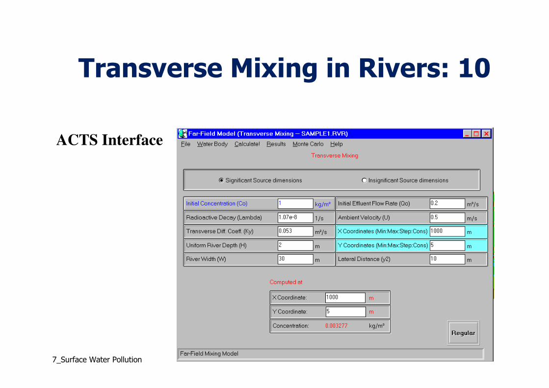
Transverse Mixing in Rivers: 10
ACTS Interface

7_Surface Water Pollution
Zones of Mixing in Rivers
� Zone A� Initial momentum and buoyancy of the discharge
is important – Mechanics of jets and plumes
� Zone B� Mixing is primarily due to river turbulence and
currents –Transverse mixing
� Zone C� Cross-sectional mixing is complete. Longitudinal
dispersion erases longitudinal gradients –Longitudinal dispersion
7_Surface Water Pollution
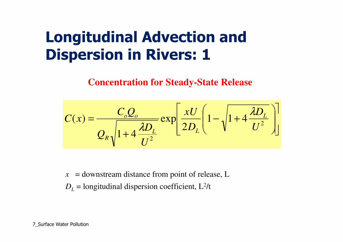
Longitudinal Advection and Dispersion in Rivers: 1
+−
+
=2
2
4112
exp
41
)(U
D
D
xU
U
DQ
QCxC L
LLR
oo λ
λ
x = downstream distance from point of release, L
DL = longitudinal dispersion coefficient, L2/t
Concentration for Steady-State Release

7_Surface Water Pollution
Longitudinal Advection and Dispersion in Rivers: 2
Longitudinal Dispersion Coefficient
According to Fischer et al. (1979), DL can be computed according to:
2 2
*
0.01L
U WD
Hu=
*5.93longitudinal
D u y=2 2
*0.011longitudinal
V BD
u y=
Shallow and wide rivers Deep and narrow rivers where bank shear is important

7_Surface Water Pollution
Longitudinal Advection and Dispersion in Rivers: 3
−
−−= t
tD
Utx
tDWH
MtxC
LL
o λπ 4
)(exp
4),(
2
For an instantaneous accidental release of a chemical mass Mo,
the time- and space-dependent concentration distribution can be
given as:
This equation is a useful first-order expression for estimating exposure
levels downstream of accidental releases.

7_Surface Water Pollution
Longitudinal Advection and Dispersion in Rivers: 4
2L LD tσ =
A useful measure of the longitudinal extent of the dispersing
pulse is its standard deviation, given by:

7_Surface Water Pollution
Longitudinal Advection and Dispersion in Rivers: 5
Cx
CD
x
CU
t
Cλ−
∂
∂+
∂
∂−=
∂
∂2
2
For a continuous source of infinite duration, the one-
dimensional advective-diffusive transport model is given as:

7_Surface Water Pollution
Longitudinal Advection and Dispersion in Rivers: 6
Continuous source of infinite duration:
C x tC Ux
Derfc
x Ut
Dt
Ux
Derfc
x Ut
Dt
o( , ) exp ( ) exp ( )= −
−
+ +
+
2 2
12 2
12
ΓΓ
ΓΓ
2/2
21
UDH
H
λ=
+=Γ

7_Surface Water Pollution
Longitudinal Advection and Dispersion in Rivers: 7
Continuous source of finite duration:
C x tC x
Uerfc
x Ut H
Dterfc
x U t H
D t
o( , ) exp
( ) ( )( )
( )=
−
− +
+
− − +
−
2
1
2
1
2
λ τ
τ

7_Surface Water Pollution
Longitudinal Advection and Dispersion in Rivers: 8
ACTS Interface
7_Surface Water Pollution
Far-Field Mixing Models
� Rivers
� Transverse mixing
� Longitudinal advection and dispersion
� Estuaries
� Small lakes and estuaries
� Oceans and great lakes

7_Surface Water Pollution
Far-Field Mixing Models
� Rivers
� Transverse mixing
� Longitudinal advection and dispersion
� Estuaries
� Small lakes and estuaries
� Oceans and great lakes

7_Surface Water Pollution
Far-Field Mixing – Small Lakes and Reservoirs
Near Field Mixing
Transverse Mixing
Longitudinal
Advection and
Dispersion
Rivers Estuaries Small Lakes and
Reservoirs
Oceans and
Great Lakes
Far Field Mixing Sediments
Pathway Models
Surface Water Pathway
Models

7_Surface Water Pollution
Small Lakes and Reservoirs: 1
� Small natural, man-made impoundments, and cooling ponds represent an extreme situation of geometric constraints and limitedadvective transport
� Half-life of chemicals considerably longerthan impoundment residence time (through flow on the order of a few days to weeks)
� Chemical concentration is essentially uniform within impoundment

7_Surface Water Pollution
Small Lakes and Reservoirs: 2
Contaminant concentration, which is a function of
time only, can be computed by:
o
o
CC
Q / Q Vλ=
+ o
Q1 exp t
/ Q Vλ
− − +

7_Surface Water Pollution
Small Lakes and Reservoirs: 3
0
0/
CC
Q Q Vλ=
+ 0/ Q

7_Surface Water Pollution
Small Lakes and Reservoirs: 4
Contaminant
Source
)(
)(
11
22
darcy
darcyo
VdLQ
VdLQ
=
=
Depth
d1
Lake Volume
V
Groundwater
flow
Contaminant
Plume
Depth
d2
L2
L1
x
yz

7_Surface Water Pollution
Small Lakes and Reservoirs: 5
ACTS Interface

7_Surface Water Pollution
Far-Field Mixing -- Estuaries
Near Field Mixing
Transverse Mixing
Longitudinal
Advection and
Dispersion
Rivers Estuaries Small Lakes and
Reservoirs
Oceans and
Great Lakes
Far Field Mixing Sediments
Pathway Models
Surface Water Pathway
Models

7_Surface Water Pollution
Estuaries: 1
Transport and dispersion processes
in estuaries are considerably more
complicated than in non-tidal rivers

7_Surface Water Pollution
Estuaries: 2
� Hydrodynamic conditions� Oscillatory tidal motion with cyclic variations in
velocity and elevation
� Vertical (baroclinic) circulations� Density differences between freshwater and
saltwater
� Wind currents in wide, shallow (bay like) estuaries
Processes to consider:

7_Surface Water Pollution
Estuaries: 3
The longitudinal distribution C(x) of any pollutant that is released in
a steady-state fashion, at a distance L upstream of the estuary
mouth, is given by (Stonmel, 1953):
++−
+−
++
−−
+−
−
+=
)11(2
exp)11(2
exp
)11(2
)(exp)11(
2
)(exp
1)(
αα
αα
α
TK
fLU
TK
fLU
TK
fULx
TK
fULx
rQ
oC
oQ
xC
Qr = fresh river flow, L3/T
α = 4λKT/Uf2
Uf = freshwater velocity, L/T
KT = tidal dispersion coefficient, L2/T

7_Surface Water Pollution
Estuaries: 4
ACTS Interface

7_Surface Water Pollution
Far-Field Mixing Models
� Rivers
� Transverse mixing
� Longitudinal advection and dispersion
� Estuaries
� Small lakes and estuaries
� Oceans and great lakes

7_Surface Water Pollution
Far-Field Mixing – Oceans and Great Lakes
Near Field Mixing
Transverse Mixing
Longitudinal
Advection and
Dispersion
Rivers Estuaries Small Lakes and
Reservoirs
Oceans and
Great Lakes
Far Field Mixing Sediments
Pathway Models
Surface Water Pathway
Models

7_Surface Water Pollution
Oceans and Great Lakes: 1
� Main feature of pollutant dispersion is unlimited extent
� Pollution analysis� Determine velocity field
� Compute dispersion of release (instantaneous or continuous)
� Neglect dynamic coupling between two phases of analysis if mass of chemical is small and buoyancy negligible

7_Surface Water Pollution
Oceans and Great Lakes: 2
� Eulerian approach for solution of advection-diffusion equation with decay term. Solution presented by Brooks (1960):
� Steady-state solution
� Uniform source of finite extent
� Steady, uniform flow

7_Surface Water Pollution
Ocean and Great Lakes: 3
Advection-Diffusion Equation
Cy
CK
yx
CU y λ−
∂
∂
∂
∂=
∂
∂
Ky = eddy diffusivity
λ = first order decay coefficient defined in terms of the
half-life (τ) of of a chemical
τλ
2ln=

7_Surface Water Pollution
Oceans and Great Lakes: 4
Definition Sketch for
Brooks Modelh
Z
U
Source
H
x
y
bUo
Co
C(x,y)
b

7_Surface Water Pollution
Oceans and Great Lakes: 5
Solution for Brooks (1960) model:
CC x
HUerf
y b U
K xerf
y b U
K x
o
y y
= −
+
−−
2
2
2
2
2exp
( / ) ( / )λ
H = vertical extent of water column, L
U = velocity of water, L/T
Ky = eddy diffusivity (constant), L2/t
λ = Radioactive decay constant, 1/T

7_Surface Water Pollution
Oceans and Great Lakes: 6
ACTS Interface

7_Surface Water Pollution
SURFACE WATER POLLUTION
Sediment Pathway Models

7_Surface Water Pollution
General Classification of Models
� Near-field mixing
� Far-field mixing
� Sediment models

7_Surface Water Pollution
Sediment Models
� Rivers
� Fletcher-Dotson model
� Onishi mixing-tank model
� Estuaries
� USNRC estuarine model
� Lakes
� USNRC two-layer lake model

7_Surface Water Pollution
Sediment Pathway Model -- Rivers
Near Field Mixing Far Field Mixing
Fletcher & Dotson Model
Onishi Model
Rivers
NRC Model
Estuaries Coastal waters
and Oceans
NRC Model
Lakes
Sediments
Pathway Models
Surface Water Pathway
Models

7_Surface Water Pollution
Sediment Pathway Models Rivers: 1
� Fletcher and Dotson Model (1971)
� Unsteady, one-dimensional, liquid pathway
� Calculates temporal and longitudinal distributions of dissolved radio-nuclide concentrations
� Calculates concentrations of chemicals attached suspended and bottom sediments

7_Surface Water Pollution
Sediment Pathway Models Rivers: 2
CQ
Q C e Q Cx t
x t
x x t t x x t t
t
i i
n
,
,
( , ) ( , )= +
− − − −
− ∑1
1∆ ∆ ∆ ∆
λ∆
Fletcher and Dotson Model (1971)
Cx,t = dissolved radio-nuclide concentration at location x, and time t
Ci = dissolved radio-nuclide concentration of the tributary
Qx,t = flow rate at location x, and time t
Qi = tributary flow rate
λ = decay coefficient

7_Surface Water Pollution
Sediment Pathway Models Rivers: 3
ACTS Interface

7_Surface Water Pollution
Sediment Pathway Models Rivers: 4
� Onishi et al. (1981) Mixing-Tank Model with Sediment Transport� River reaches are divided into segments and are
represented by a series of tanks; sediments and chemicals are concentrations completely mixed
� Chemicals and sediment contributions from point and non-point sources are treated as lateral influx that is uniformly distributed along the river reach for each segment
� Dissolved and particulate chemicals are linearly related by a distribution coefficient

7_Surface Water Pollution
Sediment Pathway Models Rivers: 5
� Onishi et al. (1981) Mixing-Tank Model with Sediment Transport--continued
� Dissolved and particulate chemicals reach their equilibrium conditions within one time step
� Particulate chemical deposition to the riverbed and re-suspension from the riverbed does not occur

7_Surface Water Pollution
Sediment Pathway Models Rivers: 6
CL1CL2
CLn
V1
C1
V2
C2
Vn
Cn
Q0
C0
Q1
C1
Q2
C2
Qn
Cn
Qn-1
Cn-1
Onishi et al. (1981) mixing tank model

7_Surface Water Pollution
Sediment Pathway Models Rivers: 7
Onishi et al. (1981) mixing tank model
Mass conservation of sediment in the nth tank
Qn = flow discharge from the nth tank
Sn = Sediment concentration in the nth tank
SLn = lateral influx of sediment into the nth tank
Vn = water volume in the nth tank
t = time
∂
∂
∂
∂
S
tS
V
V
tQ
Q S SL
V
n
n
n
n n n
n
= − +
+
+− −1 1 1

7_Surface Water Pollution
Sediment Pathway Models Rivers: 8
Onishi et al. (1981) mixing tank model
Mass balance of dissolved and particulate chemical in nth tank
{ }∂
∂ λ∂
∂
C
t V S K
S K Q C CL C L S K Q C
V C S K Ct
V S K
n
n n d
n d n n n p n n d n n
n n n d n n n d
=+
+ + + − +
− + − +
− − −1
1
1 1
1 1
1 1 1
( )
( ) ( ) ( )
( ) ( )
C K CPn d n=

7_Surface Water Pollution
Sediment Models
� Rivers
� Fletcher-Dotson model
� Onishi mixing-tank model
� Estuaries
� USNRC estuarine model
� Lakes
� USNRC two-layer lake model

7_Surface Water Pollution
Sediment Pathway Model -- Estuaries
Near Field Mixing Far Field Mixing
Fletcher & Dotson Model
Onishi Model
Rivers
NRC Model
Estuaries Coastal waters
and Oceans
NRC Model
Lakes
Sediments
Pathway Models
Surface Water Pathway
Models

7_Surface Water Pollution
Sediment Pathway ModelsEstuaries: 1
NRC Estuarine Model with Sedimentation
Sedimentation
Velocity Net Downstream
Velocity U
Water
Layer
Interface
Bed Velocity UB
d1
d2
Unmovable sediment layer
Movable sediment layer

7_Surface Water Pollution
Sediment Pathway ModelsEstuaries: 2
� Water layer is moving with a net tidally averaged downstream velocity of U
� Erodible bed is moving with a net downstream velocity, Ub
� Diffusive transport from tidal oscillations in water and sediment layers assumed to be constant with the longitudinal dispersion coefficients, Ddx and Dxb
� Sedimentation and burial occur uniformly at vertical velocity v
� dissolved and particulate chemicals are in equilibrium
Assumptions for the
NRC Estuarine Model with Sedimentation

7_Surface Water Pollution
Sediment Models
� Rivers
� Fletcher-Dotson model
� Onishi mixing-tank model
� Estuaries
� USNRC estuarine model
� Lakes
� USNRC two-layer lake model

7_Surface Water Pollution
Sediment Pathway Model -- Lakes
Near Field Mixing Far Field Mixing
Fletcher & Dotson Model
Onishi Model
Rivers
NRC Model
Estuaries Coastal waters
and Oceans
NRC Model
Lakes
Sediments
Pathway Models
Surface Water Pathway
Models

7_Surface Water Pollution
Sediment Pathway Model Lakes: 1
� Flow conditions
� Stratification and seasonal turnover
� Sedimentation interaction
� Biotic interaction
Major Processes Affecting Chemical Movement

7_Surface Water Pollution
Sediment Pathway Model Lakes: 2
NRC Two-Layer Lake Model
Sediment Layer
Decay
Decay
Water In Water Out
InterfaceSedimentation Direct Exchange Direct Exchange
Burial

7_Surface Water Pollution
Sediment Pathway Model Lakes: 3
� Water inflow and outflow are constant
� Sediment rate is constant
� Dissolved and particulate chemicals undergo decay
� The thickness of the sediment layer remains constant. (If sedimentation occurs, it is assumed that the affected portion of the original bed layer becomes inactive, and it is eliminated from the analysis)
NRC Two-Layer Lake Model Assumptions

7_Surface Water Pollution
Sediment Pathway Models Lakes: 4
ACTS Interface

7_Surface Water Pollution
Lake Pollution Application:

7_Surface Water Pollution
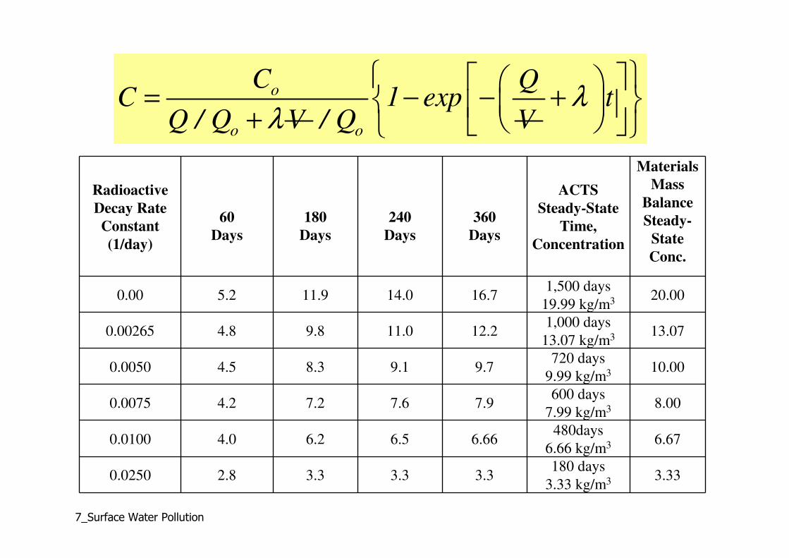
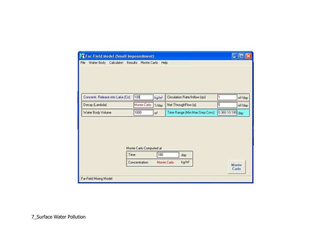
Problem:
A small “lake” is receiving a radioactive contaminant with concentration of 100 kg/m3. The circulating flow rate (qo) is 1.0 m3/day, the net flow through in the lake is 5.0 m3/day. The volume of the lake is 1000 m3. What is the concentration in the lake at 60, 180, 240, and 360 days if the radioactive decay constant has a value of?
Radioactive decay• 0.00/day (conservative) • 0.00265/day? • 0.005/day?• 0.0075/day?• 0.01/day?• 0.025/day?
V =1000m3
λ
1.0m3/d
5.0m3/d

7_Surface Water Pollution
The earlier CSTR solution :
Vo o
dCQ C QC C V
dtλ= − −
Steady state solution: 0dC
dt=
o oQ C QC C Vλ− − 0
o oQ CC
Q Vλ
=
=+
o
o o
C
Q Q V Qλ=
+
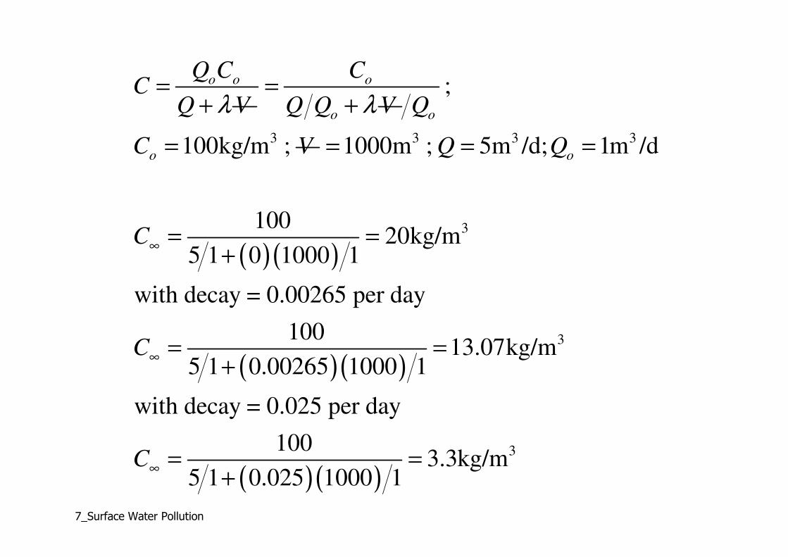
7_Surface Water Pollution
o oQ CC
Q Vλ=
+o
o
C
Q Q Vλ=
+3
;
100kg/m ;
o
o
Q
C V=
( )( )
( )( )
( )( )
3 3 3
3
3
3
1000m ; 5m /d; 1m /d
10020kg/m
5 1 0 1000 1
with decay = 0.00265 per day
10013.07kg/m
5 1 0.00265 1000 1
with decay = 0.025 per day
1003.3kg/m
5 1 0.025 1000 1
oQ Q
C
C
C
∞
∞
∞
= = =
= =+
= =+
= =+

7_Surface Water Pollution
Small Lakes and Reservoirs: 1
� Small natural, man-made impoundments, and cooling ponds represent an extreme situation of geometric constraints and limitedadvective transport
� Chemical concentration is essentially uniform within impoundment
� Time dependent analysis maybe necessary for exposure analysis and also wrt the relative values of residence time and decay.

7_Surface Water Pollution
Residence time:
1000200days 0.55
5r
Volt yrs
Q= = = =
Radioactive decay• 0.00/day (conservative) • 0.00265/day? • 0.005/day?• 0.0075/day?• 0.01/day?• 0.025/day?
Half Life• ∞ (conservative) • 261 day? • 138 day?• 92.4 day?• 69.3 day?• 27.7 day?

7_Surface Water Pollution
Small Lakes and Reservoirs: 2
Contaminant concentration, which is a function of
time only, can be computed by:
o
o
CC
Q / Q Vλ=
+ o
Q1 exp
/ Q V− − tλ
+

7_Surface Water Pollution
Small Lakes and Reservoirs: 3
0
0/
CC
Q Q Vλ∞ =
+ 0/ Q
Radioactive decay• 0.00/day (conservative) • 0.00265/day? • 0.005/day?• 0.0075/day?• 0.01/day?• 0.025/day?
Half Life• ∞ (conservative) • 261 day? • 138 day?• 92.4 day?• 69.3 day?• 27.7 day?
200r
t d=
7_Surface Water Pollution
o
o
CC
Q / Q Vλ=
+ o
Q1 exp
/ Q V− − tλ
+
Radioactive
Decay Rate
Constant
(1/day)
60
Days
180
Days
240
Days
360
Days
ACTS
Steady-State
Time,
Concentration
Materials
Mass
Balance
Steady-
State
Conc.
0.00 5.2 11.9 14.0 16.71,500 days
19.99 kg/m3 20.00
0.00265 4.8 9.8 11.0 12.21,000 days
13.07 kg/m3 13.07
0.0050 4.5 8.3 9.1 9.7720 days
9.99 kg/m3 10.00
0.0075 4.2 7.2 7.6 7.9600 days
7.99 kg/m3 8.00
0.0100 4.0 6.2 6.5 6.66480days
6.66 kg/m3 6.67
0.0250 2.8 3.3 3.3 3.3180 days
3.33 kg/m3 3.33

7_Surface Water Pollution
0 60 120 180 240 300 360TIME, IN DAYS
0.00
0.02
0.04
0.06
0.08
0.10
0.12
0.14
0.16
0.18
0.20N
OR
MA
LIZ
ED
CO
NC
EN
TR
AT
ION
(C
/CO)
SURFACE WATER ANALYSIS: FAR-FIELD MIXING -- SMALL LAKES AND RESERVOIRS
EXPLANATION
λ = 0.00 d-1
λ = 0.00265 d-1
λ = 0.005 d-1
λ = 0.0075 d-1
λ = 0.01 d-1
λ = 0.025 d-1

7_Surface Water Pollution
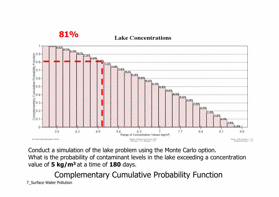
Use the same input parameters as given earlier. However, this time assume that there is a probability distribution function (PDF) for the Decay Rate Constant that is described by an EXPONENTIAL distribution. Assume the PDF has the following properties:
Minimum: 0.00265/dayMaximum: 0.025/dayMean: 0.008/dayVariance: 0.025/day2
V =1000m3
λ
1.0m3/d
5.0m3/d

7_Surface Water Pollution
Conduct a simulation of the lake problem using the Monte Carlo option. What is the probability of contaminant levels in the lake exceeding a concentration value of 5 kg/m3 at a time of 180 days.

7_Surface Water Pollution

7_Surface Water Pollution

7_Surface Water Pollution

7_Surface Water Pollution
7_Surface Water Pollution

7_Surface Water Pollution
Radioactive Decay Rate
Constant
(1/day)
180
Days
Materials Mass
Balance Steady-
State Conc.
0.00 11.9 20.00
0.00265 9.8 13.07
0.0050 8.3 10.00
0.0075 7.2 8.00
0.0100 6.2 6.67
0.0250 3.3 3.33
7_Surface Water Pollution
Complementary Cumulative Probability Function
Conduct a simulation of the lake problem using the Monte Carlo option. What is the probability of contaminant levels in the lake exceeding a concentration value of 5 kg/m3 at a time of 180 days.
81%

7_Surface Water Pollution
Small Lakes and Reservoirs:
Contaminant
Source
2 2
1 1
( )
( )
o darcy
darcy
Q L d V
Q L d V
=
=
Depth
d1
Lake Volume
V
Groundwater
flow
Contaminant
Plume
Depth
d2
L2
L1
x
yz

7_Surface Water Pollution
Transverse diffusion application
7_Surface Water Pollution
2
( , ) exp44
o o
yy
Q C y U xC x y
D x UH D Ux
λ
π
= − −
TRANSVERSE DIFFUSION: For a contaminant discharge on one side:
*0.15transverse
D u y=
2
*6.66
t
B
u yτ =
2
*6.66t t
Bx V V
u yτ= =
B
B
x
xtransverse
B
2
t
B
τ=
But also an analytical sol.:
7_Surface Water Pollution
Example: An industrial plant discharges a conservative substance at a point along the side of a river which is 2m deep 50m wide. River slope 0.02%. What is the down stream distance the pollutant starts to affect the other bank.
B
Width
x
xtransverse
B

7_Surface Water Pollution
for annings n 0.035 0.61 /M V m s= =
( ) ( ) ( )* 49.81 1.85 2 10 0.06 /h ou gR S m s−= = × =
2 501.85
2 50 2h
AR m
P
×= = =
+ +
Example: An industrial plant discharges a conservative substanceat a point along the side of a river which is 2m deep 50m wide.River slope 0.02%. What is the down stream distance the pollutant starts to affect the other bank.
( ) ( )2 / 3 1/ 21.0
h oV R Sn
=
( ) ( )* 20.15 0.15 0.06 2 0.018 /transverse
D u y m s= = =
( )
2 2
*
506.66 6.66 138750 38.54 1.6
2 0.06t
Bs days days
u yτ = = = = =
( )138750 0.61 / 84637.5 84.6transverse
x s m s m km= = =
B
B
x
xtransverse
B

7_Surface Water Pollution
2
( , ) exp44
o o
yy
Q C y U xC x y
D x UH D Ux
λ
π
= − −
Transverse diffusion model:

7_Surface Water Pollution

7_Surface Water Pollution
Diffusion only analysis ignores effluent discharge value it also ignores the initial effluent concentration.