Surface water numerical modelling for the Hunter subregion
114
A scientific collaboration between the Department of the Environment and Energy, Bureau of Meteorology, CSIRO and Geoscience Australia Surface water numerical modelling for the Hunter subregion Product 2.6.1 for the Hunter subregion from the Northern Sydney Basin Bioregional Assessment 2018
Transcript of Surface water numerical modelling for the Hunter subregion
A scientific collaboration between the Department of the Environment and Energy, Bureau of Meteorology, CSIRO and Geoscience Australia
Surface water numerical modelling for the
Hunter subregion
Product 2.6.1 for the Hunter subregion from the
Northern Sydney Basin Bioregional Assessment
2018

The Bioregional Assessment Programme
The Bioregional Assessment Programme is a transparent and accessible programme of baseline assessments that increase the available science for decision making associated with coal seam gas and large coal mines. A bioregional assessment is a scientific analysis of the ecology, hydrology, geology and hydrogeology of a bioregion with explicit assessment of the potential impacts of coal seam gas and large coal mining development on water resources. This Programme draws on the best available scientific information and knowledge from many sources, including government, industry and regional communities, to produce bioregional assessments that are independent, scientifically robust, and relevant and meaningful at a regional scale.
The Programme is funded by the Australian Government Department of the Environment and Energy. The Department of the Environment and Energy, Bureau of Meteorology, CSIRO and Geoscience Australia are collaborating to undertake bioregional assessments. For more information, visit http://www.bioregionalassessments.gov.au.
Department of the Environment and Energy
The Australian Government Department of the Environment and Energy is strengthening the regulation of coal seam gas and large coal mining development by ensuring that future decisions are informed by substantially improved science and independent expert advice about the potential water-related impacts of those developments. For more information, visit https://www.environment.gov.au/water/coal-and-coal-seam-gas/office-of-water-science.
Bureau of Meteorology
The Bureau of Meteorology is Australia’s national weather, climate and water agency. Under the Water Act 2007, the Bureau is responsible for compiling and disseminating Australia's water information. The Bureau is committed to increasing access to water information to support informed decision making about the management of water resources. For more information, visit http://www.bom.gov.au/water/.
CSIRO
Australia is founding its future on science and innovation. Its national science agency, CSIRO, is a powerhouse of ideas, technologies and skills for building prosperity, growth, health and sustainability. It serves governments, industries, business and communities across the nation. For more information, visit http://www.csiro.au.
Geoscience Australia
Geoscience Australia is Australia’s national geoscience agency and exists to apply geoscience to Australia’s most important challenges. Geoscience Australia provides geoscientific advice and information to the Australian Government to support current priorities. These include contributing to responsible resource development; cleaner and low emission energy technologies; community safety; and improving marine planning and protection. The outcome of Geoscience Australia’s work is an enhanced potential for the Australian community to obtain economic, social and environmental benefits through the application of first class research and information. For more information, visit http://www.ga.gov.au.
ISBN-PDF 978-1-9253-1559-2
Citation
Zhang YQ, Peña-Arancibia J, Viney N, Herron NF, Peeters L, Yang A, Wang W, Marvanek SP, Rachakonda PK, Ramage A, Kim S and Vaze J (2018) Surface water numerical modelling for the Hunter subregion. Product 2.6.1 for the Hunter subregion from the Northern Sydney Basin Bioregional Assessment. Department of the Environment and Energy, Bureau of Meteorology, CSIRO and Geoscience Australia, Australia. http://data.bioregionalassessments.gov.au/product/NSB/HUN/2.6.1.
Authorship is listed in relative order of contribution.
Copyright
© Commonwealth of Australia 2018 With the exception of the Commonwealth Coat of Arms and where otherwise noted, all material in this publication is provided under a Creative Commons Attribution 3.0 Australia Licence
http://www.creativecommons.org/licenses/by/3.0/au/deed.en. The Bioregional Assessment Programme requests attribution as ‘© Commonwealth of Australia (Bioregional Assessment Programme http://www.bioregionalassessments.gov.au)’.
Disclaimer
The information contained in this report is based on the best available information at the time of publication. The reader is advised that such information may be incomplete or unable to be used in any specific situation. Therefore decisions should not be made based solely on this information or without seeking prior expert professional, scientific and technical advice. The Bioregional Assessment Programme is committed to providing web accessible content wherever possible. If you are having difficulties with accessing this document please contact [email protected].
Cover photograph
Oblique view west of Muswellbrook showing Bengalla coal storage (left foreground) with irrigated agriculture and riparian vegetation either side of the Hunter River and Mount Arthur coal mine in the distance (right background), NSW, 2014
© Google earth (2015), Sinclair Knight Merz Imagery date 16 December 2008. Position 32°17’58’’ S, 150°48’51’’ E, elevation 136 m, eye altitude 1.59 km
Surface water numerical modelling for the Hunter subregion | i
Executive summary
Coal resource development can potentially affect water-dependent assets (either negatively or
positively) through impacts on surface water hydrology. This product presents the modelled
hydrological changes in response to likely coal resource development in the Hunter subregion
after December 2012.
To quantify impacts of coal resource development in the Hunter subregion, two potential futures
are considered in a bioregional assessment (BA):
baseline coal resource development (baseline): a future that includes all coal mines and coal
seam gas (CSG) fields that are commercially producing as at December 2012
coal resource development pathway (CRDP): a future that includes all coal mines and CSG
fields that are in the baseline as well as those that are expected to begin commercial
production after December 2012.
The difference in results between CRDP and baseline is the change that is primarily reported in a
BA. This change is due to the additional coal resource development – all coal mines and CSG fields
in the Hunter subregion, including expansions of baseline operations, that are expected to begin
commercial production after December 2012.
In the Hunter subregion, coal mining has been occurring for over 100 years. The BA for the Hunter
subregion includes 42 baseline mines and 22 additional coal resource developments. Twelve
baseline mines were not modelled because they were within the tidal zone of the river system or
under Lake Macquarie and adjacent urban areas, did not have associated additional coal resource
developments and/or due to lack of data. Five additional coal resource developments were not
modelled due to lack of data, low likelihood of impact at the surface or being under Lake
Macquarie. Therefore, the surface water numerical modelling in the Hunter subregion includes 47
mines comprising 30 baseline mines and 17 additional coal resource developments. In the Hunter
subregion, there are no CSG fields in the CRDP.
Surface water modelling of the Hunter subregion follows the companion submethodology M06 for
surface water modelling. In particular, the modelling is undertaken as follows:
The model includes rainfall-runoff modelling and river modelling.
Streamflow inputs are obtained by accumulating output from the Australian Water
Resources Assessment (AWRA) landscape model (AWRA-L) for input into the AWRA river
model (AWRA-R).
Changes in baseflow from the Hunter subregion groundwater model are also fed into the
AWRA-R model at points along the river network.
The river model integrates the potential baseflow and runoff changes due to the modelled
coal resource developments.

ii | Surface water numerical modelling for the Hunter subregion
The modelling domain includes part of the Hunter river basin and part of the Macquarie-
Tuggerah lakes basin.
Daily streamflow predictions are produced at 65 model nodes.
The model simulation period is from 2013 to 2102.
Evaluation of the model assumptions on predictions shows that most assumptions are unlikely to
have a significant effect on predictions. However, predictions are sensitive to the implementation
of the CRDP – particularly in catchments where the mine footprint is a large fraction of total
catchment area. Predictions may also be affected by the criteria for choosing the most appropriate
parameter combinations and representation of river regulation in the river model.
The surface water modelling results show that the additional coal resource development in the
Hunter subregion has the potential to cause large changes in the flow regime of some streams.
This is particularly evident for the hydrological response variables that characterise high-
streamflow conditions at model nodes where the additional coal resource developments cover a
large proportion of the contributing area.
In general, the hydrological effects attributable to the additional coal resource development are
greater in the small tributaries of the Hunter River than along the river itself. The biggest impacts
(flow reductions of up to 80%) occur at nodes 7 to 9 (Loders Creek, including Doctors Creek),
which enter the Hunter River just upstream of Singleton, and at nodes 52 (Dry Creek) and 55
(unnamed creek) in the vicinity of Muswellbrook. The catchments of nodes 7 to 9 include the
Bulga and Mount Thorley–Warkworth mines, while the catchments of nodes 52 and 55 include the
Bengalla and Mount Pleasant mines. Other nodes with substantial percentage changes in the high-
streamflow hydrological response variables are nodes 26, 27, 29 and 35. The first three of these
nodes are all located in the vicinity of the Glendell, Integra, Liddell and Mount Owen mines, while
the catchment of node 35 includes parts of the Drayton South and Mount Arthur mines. All these
nodes have relatively small catchment areas. Although there are bigger predicted changes in
maximum raw change (amax) at nodes further downstream, the proportional impacts of these
changes are diluted by relatively unaffected inflows. The prediction that the biggest changes occur
downstream of multiple mine developments highlights the cumulative nature of potential
hydrological changes.
The changes to the low-streamflow hydrological response variables attributable to the additional
coal resource development appear to be slightly larger than those to the high-streamflow
hydrological response variables. However, the uncertainty in the predicted change and the timing
of the maximum change are greater for the low-streamflow variables.
There is a substantial change in the low-streamflow hydrological response variables in the two
nodes of the Wyong river basin. These nodes are located near the proposed Wallarah 2 and
Mandalong underground mines. In the most heavily affected year, these reductions in baseflow
are predicted to turn a perennial stream into one that flows on only about 40% of days. Although
this is a large reduction, it must be remembered that the projections presented in Section 2.6.1.6
are for the worst-case year during the entire simulation period (2013 to 2102). There is no
implication, particularly for the low-flow variables, that the changes will be this severe in every
year. When local hydrogeological and geological data are used to constrain groundwater model

Surface water numerical modelling for the Hunter subregion | iii
results in the Wyong river basin, groundwater drawdowns are predicted to be smaller and less
extensive, resulting in little to no changes in baseflow (product 2.6.2). Where results from the
regional scale modelling flag a risk of large hydrological changes from additional coal resource
development, a more locally relevant assessment of potential hydrological changes should be
made using local information to constrain the set of regional simulations to those representative
of the local conditions.
The results suggest that changes to low-streamflow characteristics are caused by a combination of
the instantaneous impact of interception from the additional mine footprints and the cumulative
impact on baseflow over time caused by watertable drawdown. The changes to high-streamflow
characteristics are dominated by direct interception of runoff.
The surface water numerical modelling described in this product needs to be considered in
conjunction with the groundwater numerical modelling (product 2.6.2). Together they provide key
inputs to the receptor impact modelling (product 2.7) and underpin the analysis of impacts on
landscape classes and assets in product 3-4 (impact and risk analysis).

iv | Surface water numerical modelling for the Hunter subregion

Surface water numerical modelling for the Hunter subregion | v
Contents
Executive summary ..................................................................................................................... i
Contributors to the Technical Programme .................................................................................. x
Acknowledgements .................................................................................................................. xii
Currency of scientific results .................................................................................................... xiii
Introduction ............................................................................................................................... 1
The Bioregional Assessment Programme ................................................................................... 1
Methodologies ............................................................................................................................ 3
Technical products ...................................................................................................................... 5
About this technical product ...................................................................................................... 8
References .................................................................................................................................. 8
2.6.1.1 Methods ................................................................................................................. 10
2.6.1.1.1 Background and context ............................................................................................ 10
2.6.1.1.2 Surface water numerical modelling .......................................................................... 11
2.6.1.1.3 Model sequencing ..................................................................................................... 12
2.6.1.1.4 Integration with sensitivity and uncertainty analysis workflow ............................... 13
References ................................................................................................................................ 14
2.6.1.2 Review of existing models ....................................................................................... 17
References ................................................................................................................................ 18
2.6.1.3 Model development ................................................................................................ 19
2.6.1.3.1 Spatial and temporal dimensions .............................................................................. 19
2.6.1.3.2 Location of model nodes ........................................................................................... 20
2.6.1.3.3 Choice of seasonal scaling factors for climate trend ................................................. 23
2.6.1.3.4 Representing the hydrological changes from mining ............................................... 24
2.6.1.3.5 Modelling river management .................................................................................... 29
2.6.1.3.6 Rules to simulate industry water discharge .............................................................. 29
References ................................................................................................................................ 29
Datasets ................................................................................................................................... 30
2.6.1.4 Calibration .............................................................................................................. 33
2.6.1.4.1 Australian Water Resources Assessment landscape model ..................................... 33
2.6.1.4.2 Australian Water Resources Assessment river model .............................................. 40
References ................................................................................................................................ 52
Datasets ................................................................................................................................... 53
vi | Surface water numerical modelling for the Hunter subregion
2.6.1.5 Uncertainty ............................................................................................................. 55
2.6.1.5.1 Quantitative uncertainty analysis ............................................................................. 55
2.6.1.5.2 Qualitative uncertainty analysis ................................................................................ 58
References ................................................................................................................................ 63
2.6.1.6 Prediction ............................................................................................................... 65
2.6.1.6.1 Introduction ............................................................................................................... 65
2.6.1.6.2 Results analysis .......................................................................................................... 67
2.6.1.6.3 Summary and discussion ........................................................................................... 85
2.6.1.6.4 Defining thresholds of hydrological change .............................................................. 87
References ................................................................................................................................ 92
Datasets ................................................................................................................................... 92
Glossary ................................................................................................................................... 94
Surface water numerical modelling for the Hunter subregion | vii
Figures
Figure 1 Schematic diagram of the bioregional assessment methodology .................................... 2
Figure 2 Technical products and submethodologies associated with each component of a
bioregional assessment ................................................................................................................... 6
Figure 3 Model sequence for the Hunter subregion .................................................................... 13
Figure 4 Hunter subregion surface water modelling domain, location of model nodes and
maximum extents of mine footprints ........................................................................................... 21
Figure 5 Schematic representation of the node-link network for Hunter subregion surface water
modelling....................................................................................................................................... 22
Figure 6 Time series of observed and projected annual precipitation averaged over the Hunter
subregion ...................................................................................................................................... 24
Figure 7 Time series of the mine footprint area for Ashton Coal Mine’s open-cut and
underground mines ....................................................................................................................... 25
Figure 8 The 14 streamflow gauging stations used for AWRA-L model calibration and their
contributing areas ......................................................................................................................... 35
Figure 9 Summary of two AWRA-L model calibrations for the Hunter subregion ....................... 37
Figure 10 Summary of model bias for the nine simulated hydrological response variables for
high-streamflow and low-streamflow calibrations ....................................................................... 39
Figure 11 Streamflow gauging stations and ungauged upland headwater nodes used for AWRA-
R model calibration and their contributing areas ......................................................................... 42
Figure 12 Summary of two AWRA-R model calibrations for the Hunter River ............................. 44
Figure 13 Flow duration curves for selected stations in Wollombi Brook (210004) and
Goulburn River (210006, 210016, 210031) for AWRA-R high-streamflow calibration (top row)
and AWRA-R low-streamflow calibration (bottom row), respectively ......................................... 45
Figure 14 Summary of performance of the nine simulated hydrological response variables
obtained using the two AWRA-R model calibrations ................................................................... 47
Figure 15 Example of IQQM and simulated monthly irrigation diversions for four reaches in
the Hunter River ............................................................................................................................ 49
Figure 16 Observed and AWRA-R simulated monthly dam storage volume for (a) Glenbawn
Dam and (c) Glennies Creek Dam; and IQQM and AWRA-R simulated monthly releases for
(b) Glenbawn Dam and (d) Glennies Creek Dam .......................................................................... 50
viii | Surface water numerical modelling for the Hunter subregion
Figure 17 Percentage error for monthly dam storage volumes for Glenbawn Dam and for
Glennies Creek Dam ...................................................................................................................... 51
Figure 18 Observed and AWRA-R simulated allocations for the AWRA-R Hunter river system .. 51
Figure 19 Hydrological changes due to additional coal resource development on annual flow
(AF) at the 65 model nodes within the Hunter subregion ............................................................ 68
Figure 20 Hydrological changes due to additional coal resource development on daily
streamflow at the 99th percentile (P99) at the 65 model nodes within the Hunter subregion .. 70
Figure 21 Hydrological changes due to additional coal resource development on interquartile
range (IQR) at the 65 model nodes within the Hunter subregion ................................................ 72
Figure 22 Hydrological changes due to additional coal resource development on high-flow days
(FD) at the 65 model nodes within the Hunter subregion ............................................................ 74
Figure 23 Hydrological changes due to additional coal resource development on daily
streamflow at the 1st percentile (P01) at the 65 model nodes within the Hunter subregion ..... 76
Figure 24 Hydrological changes due to the additional coal resource development on the
number of zero-flow days (ZFD) at the 65 model nodes within the Hunter subregion ............... 78
Figure 25 Hydrological changes due to the additional coal resource development on the
number of low-flow days (LFD) at the 65 model nodes within the Hunter subregion ................ 80
Figure 26 Hydrological changes due to the additional coal resource development on the
number of low-flow spells (LFS) at the 65 model nodes within the Hunter subregion ............... 82
Figure 27 Hydrological changes due to the additional coal resource development on the length
of longest low-flow spell (LLFS) at the 65 model nodes within the Hunter subregion ................ 84
Figure 28 Model nodes and links with changes in at least one hydrological response variable
due to additional coal resource development that exceed specified thresholds ........................ 91

Surface water numerical modelling for the Hunter subregion | ix
Tables
Table 1 Methodologies ................................................................................................................... 4
Table 2 Technical products delivered for the Hunter subregion .................................................... 7
Table 3 List of 15 global climate models (GCMs) and their predicted change in mean annual
precipitation across the Hunter subregion per degree of global warming .................................. 23
Table 4 Contributing area and maximum mine footprint area to each model node
in AWRA-R ..................................................................................................................................... 27
Table 5 Calibration statistics for the 14 AWRA-L calibration catchments .................................... 38
Table 6 Hydrological response variables used to characterise hydrological changes of coal
resource development .................................................................................................................. 39
Table 7 Summary of AWRA-R calibration for the 20 reaches in the Hunter subregion ............... 46
Table 8 Summary of AWRA-R irrigation calibration for nine reaches in the Hunter subregion ... 48
Table 9 Summary of AWRA-L and AWRA-R parameters for uncertainty analysis ........................ 56
Table 10 Qualitative uncertainty analysis as used for the Hunter subregion surface water
model ............................................................................................................................................ 59
Table 11 Change in hydrological response variable (column) relative to its threshold at each
model node (row) due to additional coal resource development ............................................... 88

x | Surface water numerical modelling for the Hunter subregion
Contributors to the Technical Programme
The following individuals have contributed to the Technical Programme, the part of the
Bioregional Assessment Programme that undertakes bioregional assessments.
Role or team Contributor(s)
Assistant Secretary Department of the Environment and Energy: Matthew Whitfort
Programme Director Department of the Environment and Energy: Anthony Swirepik
Technical Programme Director Bureau of Meteorology: Julie Burke
Projects Director CSIRO: David Post
Principal Science Advisor Department of the Environment and Energy: Peter Baker
Science Directors CSIRO: Brent Henderson
Geoscience Australia: Steven Lewis
Integration Bureau of Meteorology: Richard Mount (Integration Leader)
CSIRO: Becky Schmidt
Programme management Bureau of Meteorology: Louise Minty
CSIRO: Paul Bertsch, Warwick McDonald
Geoscience Australia: Stuart Minchin
Project Leaders CSIRO: Alexander Herr, Kate Holland, Tim McVicar, David Rassam
Geoscience Australia: Tim Evans
Bureau of Meteorology: Natasha Herron
Assets and receptors Bureau of Meteorology: Richard Mount (Discipline Leader)
Department of the Environment and Energy: Glenn Johnstone, Wasantha Perera, Jin Wang
Bioregional Assessment Information Platform
Bureau of Meteorology: Lakshmi Devanathan (Team Leader), Derek Chen,
Trevor Christie-Taylor, Melita Dahl, Angus MacAulay, Christine Price,
Paul Sheahan, Kellie Stuart,
CSIRO: Peter Fitch, Ashley Sommer
Geoscience Australia: Neal Evans
Communications Bureau of Meteorology: Jessica York
CSIRO: Clare Brandon
Department of the Environment and Energy: John Higgins, Miriam McMillan, Milica Milanja
Geoscience Australia: Aliesha Lavers
Coordination Bureau of Meteorology: Brendan Moran, Eliane Prideaux, Sarah van Rooyen
CSIRO: Ruth Palmer
Department of the Environment and Energy: Anisa Coric, Lucy Elliott, James Hill, Andrew Stacey, David Thomas, Emily Turner
Ecology CSIRO: Anthony O'Grady (Discipline Leader), Caroline Bruce, Tanya Doody,
Brendan Ebner, Craig MacFarlane, Patrick Mitchell, Justine Murray, Chris Pavey, Jodie Pritchard, Nat Raisbeck-Brown, Ashley Sparrow

Surface water numerical modelling for the Hunter subregion | xi
Role or team Contributor(s)
Geology CSIRO: Deepak Adhikary, Emanuelle Frery, Mike Gresham, Jane Hodgkinson,
Zhejun Pan, Matthias Raiber, Regina Sander, Paul Wilkes
Geoscience Australia: Steven Lewis (Discipline Leader)
Geographic information systems
CSIRO: Jody Bruce, Debbie Crawford, Dennis Gonzales, Mike Gresham,
Steve Marvanek, Arthur Read
Geoscience Australia: Adrian Dehelean, Joe Bell
Groundwater modelling CSIRO: Russell Crosbie (Discipline Leader), Tao Cui, Warrick Dawes, Lei Gao, Sreekanth Janardhanan, Luk Peeters, Praveen Kumar Rachakonda,
Wolfgang Schmid, Saeed Torkzaban, Chris Turnadge, Andy Wilkins, Binzhong Zhou
Hydrogeology Geoscience Australia: Tim Ransley (Discipline Leader), Chris Harris-Pascal,
Jessica Northey, Emily Slatter
Information management Bureau of Meteorology: Brendan Moran (Team Leader), Christine Panton
CSIRO: Qifeng Bai, Simon Cox, Phil Davies, Geoff Hodgson, Brad Lane, Ben Leighton, David Lemon, Trevor Pickett, Shane Seaton, Ramneek Singh, Matt Stenson
Geoscience Australia: Matti Peljo
Information model and impact analysis
Bureau of Meteorology: Carl Sudholz (Project Manager), Mark Dyall, Michael Lacey, Brett Madsen, Eliane Prideaux
Geoscience Australia: Trevor Tracey-Patte
Products CSIRO: Becky Schmidt (Products Manager), Maryam Ahmad, Helen Beringen, Clare Brandon, Heinz Buettikofer, Sonja Chandler, Siobhan Duffy, Karin Hosking, Allison Johnston, Maryanne McKay, Linda Merrin, Sally Tetreault-Campbell, Catherine Ticehurst
Geoscience Australia: Penny Kilgour, Kathryn Owen
Risk and uncertainty CSIRO: Simon Barry (Discipline Leader), Jeffrey Dambacher, Rob Dunne, Jess Ford, Keith Hayes, Geoff Hosack, Adrien Ickowicz, Warren Jin, Dan Pagendam
Surface water hydrology CSIRO: Neil Viney (Discipline Leader), Santosh Aryal, Mat Gilfedder, Fazlul Karim, Lingtao Li, Dave McJannet, Jorge Luis Peña-Arancibia, Tom Van Niel, Jai Vaze,
Bill Wang, Ang Yang, Yongqiang Zhang

xii | Surface water numerical modelling for the Hunter subregion
Acknowledgements
This technical product was reviewed by several groups:
Senior Science Leaders: David Post (Projects Director), Steven Lewis (Science Director,
Geoscience Australia), Brent Henderson (Science Director, CSIRO), Becky Schmidt (Products
Manager)
Technical Assurance Reference Group: Chaired by Peter Baker (Principal Science Advisor,
Department of the Environment and Energy), this group comprises officials from the NSW,
Queensland, South Australian and Victorian governments
Additional Reviewers: Mark Simons (NSW Department of Primary Industries (Office of
Water)) Abi Javam (NSW Department of Primary Industries (Office of Water)).

Surface water numerical modelling for the Hunter subregion | xiii
Currency of scientific results
The modelling results contained in this product were completed in August 2016 using the best
available data, models and approaches available at that time. The product content was completed
in August 2017.
All products in the model-data analysis, impact and risk analysis, and outcome synthesis (see
Figure 1) were published as a suite when completed.

xiv | Surface water numerical modelling for the Hunter subregion

Surface water numerical modelling for the Hunter subregion | 1
Introduction
The Independent Expert Scientific Committee on Coal Seam Gas and Large Coal Mining
Development (IESC) was established to provide advice to the federal Minister for the Environment
on potential water-related impacts of coal seam gas (CSG) and large coal mining developments
(IESC, 2015).
Bioregional assessments (BAs) are one of the key mechanisms to assist the IESC in developing this
advice so that it is based on best available science and independent expert knowledge.
Importantly, technical products from BAs are also expected to be made available to the public,
providing the opportunity for all other interested parties, including government regulators,
industry, community and the general public, to draw from a single set of accessible information. A
BA is a scientific analysis, providing a baseline level of information on the ecology, hydrology,
geology and hydrogeology of a bioregion with explicit assessment of the potential impacts of CSG
and coal mining development on water resources.
The IESC has been involved in the development of Methodology for bioregional assessments of the
impacts of coal seam gas and coal mining development on water resources (the BA methodology;
Barrett et al., 2013) and has endorsed it. The BA methodology specifies how BAs should be
undertaken. Broadly, a BA comprises five components of activity, as illustrated in Figure 1. Each BA
is different, due in part to regional differences, but also in response to the availability of data,
information and fit-for-purpose models. Where differences occur, these are recorded, judgments
exercised on what can be achieved, and an explicit record is made of the confidence in the
scientific advice produced from the BA.
The Bioregional Assessment Programme
The Bioregional Assessment Programme is a collaboration between the Department of the
Environment and Energy, the Bureau of Meteorology, CSIRO and Geoscience Australia. Other
technical expertise, such as from state governments or universities, is also drawn on as required.
For example, natural resource management groups and catchment management authorities
identify assets that the community values by providing the list of water-dependent assets, a key
input.
The Technical Programme, part of the Bioregional Assessment Programme, has undertaken BAs
for the following bioregions and subregions (see
http://www.bioregionalassessments.gov.au/assessments for a map and further information):
the Galilee, Cooper, Pedirka and Arckaringa subregions, within the Lake Eyre Basin bioregion
the Maranoa-Balonne-Condamine, Gwydir, Namoi and Central West subregions, within the
Northern Inland Catchments bioregion
the Clarence-Moreton bioregion
the Hunter and Gloucester subregions, within the Northern Sydney Basin bioregion

2 | Surface water numerical modelling for the Hunter subregion
the Sydney Basin bioregion
the Gippsland Basin bioregion.
Technical products (described in a later section) will progressively be delivered throughout the
Programme.
Figure 1 Schematic diagram of the bioregional assessment methodology
The methodology comprises five components, each delivering information into the bioregional assessment and building on prior components, thereby contributing to the accumulation of scientific knowledge. The small grey circles indicate activities external to the bioregional assessment. Risk identification and risk likelihoods are conducted within a bioregional assessment (as part of Component 4) and may contribute activities undertaken externally, such as risk evaluation, risk assessment and risk treatment. Source: Figure 1 in Barrett et al. (2013), © Commonwealth of Australia

Surface water numerical modelling for the Hunter subregion | 3
Methodologies
The overall scientific and intellectual basis of the BAs is provided in the BA methodology (Barrett
et al., 2013). Additional guidance is required, however, about how to apply the BA methodology to
a range of subregions and bioregions. To this end, the teams undertaking the BAs have developed
and documented detailed scientific submethodologies (Table 1), in the first instance, to support
the consistency of their work across the BAs and, secondly, to open the approach to scrutiny,
criticism and improvement through review and publication. In some instances, methodologies
applied in a particular BA may differ from what is documented in the submethodologies.
The relationship of the submethodologies to BA components and technical products is illustrated
in Figure 2. While much scientific attention is given to assembling and transforming information,
particularly through the development of the numerical, conceptual and receptor impact models,
integration of the overall assessment is critical to achieving the aim of the BAs. To this end, each
submethodology explains how it is related to other submethodologies and what inputs and
outputs are required. They also define the technical products and provide guidance on the content
to be included. When this full suite of submethodologies is implemented, a BA will result in a
substantial body of collated and integrated information for a subregion or bioregion, including
new information about the potential impacts of coal resource development on water and water-
dependent assets.

4 | Surface water numerical modelling for the Hunter subregion
Table 1 Methodologies
Each submethodology is available online at http://data.bioregionalassessments.gov.au/submethodology/XXX, where ‘XXX’ is replaced by the code in the first column. For example, the BA methodology is available at http://data.bioregionalassessments.gov.au/submethodology/bioregional-assessment-methodology and submethodology M02 is available at http://data.bioregionalassessments.gov.au/submethodology/M02. Submethodologies might be added in the future.
Code Proposed title Summary of content
bioregional-assessment-methodology
Methodology for bioregional assessments of the impacts of coal seam gas and coal mining development on water resources
A high-level description of the scientific and intellectual basis for a consistent approach to all bioregional assessments
M02 Compiling water-dependent assets Describes the approach for determining water-dependent assets
M03 Assigning receptors to water-dependent assets
Describes the approach for determining receptors associated with water-dependent assets
M04 Developing a coal resource development pathway
Specifies the information that needs to be collected and reported about known coal and coal seam gas resources as well as current and potential resource developments
M05 Developing the conceptual model of causal pathways
Describes the development of the conceptual model of causal pathways, which summarises how the ‘system’ operates and articulates the potential links between coal resource development and changes to surface water or groundwater
M06 Surface water modelling Describes the approach taken for surface water modelling
M07 Groundwater modelling Describes the approach taken for groundwater modelling
M08 Receptor impact modelling Describes how to develop receptor impact models for assessing potential impact to assets due to hydrological changes that might arise from coal resource development
M09 Propagating uncertainty through models
Describes the approach to sensitivity analysis and quantification of uncertainty in the modelled hydrological changes that might occur in response to coal resource development
M10 Impacts and risks Describes the logical basis for analysing impact and risk
M11 Systematic analysis of water-related hazards associated with coal resource development
Describes the process to identify potential water-related hazards from coal resource development

Surface water numerical modelling for the Hunter subregion | 5
Technical products
The outputs of the BAs include a suite of technical products presenting information about the
ecology, hydrology, hydrogeology and geology of a bioregion and the potential impacts of CSG and
coal mining developments on water resources, both above and below ground. Importantly, these
technical products are available to the public, providing the opportunity for all interested parties,
including community, industry and government regulators, to draw from a single set of accessible
information when considering CSG and large coal mining developments in a particular area.
The information included in the technical products is specified in the BA methodology. Figure 2
shows the relationship of the technical products to BA components and submethodologies.
Table 2 lists the content provided in the technical products, with cross-references to the part of
the BA methodology that specifies it. The red outlines in both Figure 2 and Table 2 indicate the
information included in this technical product.
Technical products are delivered as reports (PDFs). Additional material is also provided, as
specified by the BA methodology:
unencumbered data syntheses and databases
unencumbered tools, model code, procedures, routines and algorithms
unencumbered forcing, boundary condition, parameter and initial condition datasets
lineage of datasets (the origin of datasets and how they are changed as the BA progresses)
gaps in data and modelling capability.
In this context, unencumbered material is material that can be published according to conditions
in the licences or any applicable legislation. All reasonable efforts were made to provide all
material under a Creative Commons Attribution 3.0 Australia Licence.
Technical products, and the additional material, are available online at
http://www.bioregionalassessments.gov.au.
The Bureau of Meteorology archives a copy of all datasets used in the BAs. This archive includes
datasets that are too large to be stored online and datasets that are encumbered. The community
can request a copy of these archived data at http://www.bioregionalassessments.gov.au.

6 | Surface water numerical modelling for the Hunter subregion
Figure 2 Technical products and submethodologies associated with each component of a bioregional assessment
In each component (Figure 1) of a bioregional assessment, a number of technical products (coloured boxes, see also Table 2) are potentially created, depending on the availability of data and models. The light grey boxes indicate submethodologies (Table 1) that specify the approach used for each technical product. The red outline indicates this technical product. The BA methodology (Barrett et al., 2013) specifies the overall approach.

Surface water numerical modelling for the Hunter subregion | 7
Table 2 Technical products delivered for the Hunter subregion
For each subregion in the Northern Sydney Basin Bioregional Assessment, technical products are delivered online at http://www.bioregionalassessments.gov.au, as indicated in the ‘Type’ columna. Other products – such as datasets, metadata, data visualisation and factsheets – are provided online. There is no product 1.4. Originally this product was going to describe the receptor register and application of landscape classes as per Section 3.5 of the BA methodology, but this information is now included in product 2.3 (conceptual modelling) and used in product 2.6.1 (surface water numerical modelling) and product 2.6.2 (groundwater numerical modelling). There is no product 2.4. Originally this product was going to include two- and three-dimensional representations as per Section 4.2 of the BA methodology, but these are instead included in products such as product 2.3 (conceptual modelling), product 2.6.1 (surface water numerical modelling) and product 2.6.2 (groundwater numerical modelling).
Component Product code
Title Section in the BA methodologyb
Typea
Component 1: Contextual information for the Hunter subregion
1.1 Context statement 2.5.1.1, 3.2 PDF, HTML
1.2 Coal and coal seam gas resource assessment
2.5.1.2, 3.3 PDF, HTML
1.3 Description of the water-dependent asset register
2.5.1.3, 3.4 PDF, HTML, register
1.5 Current water accounts and water quality
2.5.1.5 PDF, HTML
1.6 Data register 2.5.1.6 Register
Component 2: Model-data analysis for the Hunter subregion
2.1-2.2 Observations analysis, statistical analysis and interpolation
2.5.2.1, 2.5.2.2 PDF, HTML
2.3 Conceptual modelling 2.5.2.3, 4.3 PDF, HTML
2.5 Water balance assessment 2.5.2.4 PDF, HTML
2.6.1 Surface water numerical modelling 4.4 PDF, HTML
2.6.2 Groundwater numerical modelling 4.4 PDF, HTML
2.7 Receptor impact modelling 2.5.2.6, 4.5 PDF, HTML
Component 3 and Component 4: Impact and risk analysis for the Hunter subregion
3-4 Impact and risk analysis 5.2.1, 2.5.4, 5.3 PDF, HTML
Component 5: Outcome synthesis for the Hunter subregion
5 Outcome synthesis 2.5.5 PDF, HTML
aThe types of products are as follows: ● ‘PDF’ indicates a PDF document that is developed by the Northern Sydney Basin Bioregional Assessment using the structure, standards and format specified by the Programme. ● ‘HTML’ indicates the same content as in the PDF document, but delivered as webpages. ● ‘Register’ indicates controlled lists that are delivered using a variety of formats as appropriate.
bMethodology for bioregional assessments of the impacts of coal seam gas and coal mining development on water resources (Barrett et al., 2013)
8 | Surface water numerical modelling for the Hunter subregion
About this technical product
The following notes are relevant only for this technical product.
All reasonable efforts were made to provide all material under a Creative Commons
Attribution 3.0 Australia Licence.
All maps created as part of this BA for inclusion in this product used the Albers equal area
projection with a central meridian of 151.0° East for the Northern Sydney Basin bioregion
and two standard parallels of –18.0° and –36.0°.
Visit http://bioregionalassessments.gov.au to access metadata (including copyright,
attribution and licensing information) for datasets cited or used to make figures in this
product.
In addition, the datasets are published online if they are unencumbered (able to be
published according to conditions in the licence or any applicable legislation). The Bureau of
Meteorology archives a copy of all datasets used in the BAs. This archive includes datasets
that are too large to be stored online and datasets that are encumbered. The community can
request a copy of these archived data at http://www.bioregionalassessments.gov.au.
The citation details of datasets are correct to the best of the knowledge of the Bioregional
Assessment Programme at the publication date of this product. Readers should use the
hyperlinks provided to access the most up-to-date information about these data; where
there are discrepancies, the information provided online should be considered correct. The
dates used to identify Bioregional Assessment Source Datasets are the dataset’s published
date. Where the published date is not available, the last updated date or created date is
used. For Bioregional Assessment Derived Datasets, the created date is used.
References
Barrett DJ, Couch CA, Metcalfe DJ, Lytton L, Adhikary DP and Schmidt RK (2013) Methodology for
bioregional assessments of the impacts of coal seam gas and coal mining development on
water resources. A report prepared for the Independent Expert Scientific Committee on Coal
Seam Gas and Large Coal Mining Development through the Department of the Environment.
Department of the Environment, Australia. Viewed 2 March 2018,
http://data.bioregionalassessments.gov.au/submethodology/bioregional-assessment-
methodology.
IESC (2015) Information guidelines for the Independent Expert Scientific Committee advice on coal
seam gas and large coal mining development proposals. Independent Expert Scientific
Committee on Coal Seam Gas and Large Coal Mining Development, Australia. Viewed 2
March 2018, http://www.iesc.environment.gov.au/publications/information-guidelines-
independent-expert-scientific-committee-advice-coal-seam-gas.
Surface water numerical modelling for the Hunter subregion | 9
2.6.1 Surface water numerical modelling for the Hunter subregion
Coal and coal seam gas (CSG) development can potentially affect water-dependent assets (either
negatively or positively) through impacts on surface water hydrology. This product presents the
modelling of surface water hydrology within the Hunter subregion.
First, the methods are summarised and existing models reviewed, followed by details regarding
the development and calibration of the model. The product concludes with predictions of
hydrological response variables, including uncertainty.
Results are reported for the two potential futures considered in a bioregional assessment:
baseline coal resource development (baseline): a future that includes all coal mines and coal
seam gas (CSG) fields that are commercially producing as of December 2012
coal resource development pathway (CRDP): a future that includes all coal mines and CSG
fields that are in the baseline as well as those that are expected to begin commercial
production after December 2012.
The difference in results between CRDP and baseline is the change that is primarily reported in a
bioregional assessment. This change is due to the additional coal resource development – all coal
mines and CSG fields, including expansions of baseline operations, that are expected to begin
commercial production after December 2012.
This product reports results for only those developments in the baseline and CRDP that can be
modelled. Results generated at model nodes are interpolated to estimate potential hydrological
changes for surface water. Similarly, potential hydrological changes are estimated for groundwater
in product 2.6.2 (groundwater numerical modelling). Product 3-4 (impact and risk analysis) then
reports impacts on landscape classes and water-dependent assets arising from these hydrological
changes.
The hydrological results from both product 2.6.1 (surface water numerical modelling) and product
2.6.2 (groundwater numerical modelling) are used to assess water balances, reported in product
2.5 (water balance assessment).

2.6.1.1 Methods
10 | Surface water numerical modelling for the Hunter subregion
Co
mp
on
ent
2: M
od
el-d
ata
anal
ysis
fo
r th
e H
un
ter
sub
regi
on
2.6.1.1 Methods
Summary
A generic methodology for surface water modelling in the Bioregional Assessment
Programme appears in companion submethodology M06 (as listed in Table 1) (Viney, 2016).
This section describes the departures from that generic methodology that have been applied
in the Hunter subregion.
Surface water modelling of the Hunter subregion includes landscape water balance modelling
and river modelling. Streamflow inputs are obtained by accumulating output from the
Australian Water Resources Assessment (AWRA) landscape model (AWRA-L) for input into the
AWRA river model (AWRA-R). Baseflow contributions from the Hunter subregion
groundwater model are also fed into the AWRA-R model at points along the river network.
Thus, the river model integrates the impacts of mining development on groundwater and
surface water systems.
2.6.1.1.1 Background and context
The numerical surface water modelling in a bioregional assessment has a very specific objective: to
probabilistically evaluate potential hydrological change in the coal resource development pathway
(CRDP) relative to the baseline at specified locations in the subregion to inform the impact and risk
analysis reported in product 3-4. Outputs from the surface water modelling are also used as inputs
to product 2.7 (receptor impact modelling) to facilitate evaluation of the cumulative impacts of
mining on water-dependent ecological and economic assets.
The probabilistic aspect of the analysis implies that modelling does not provide a single best
estimate of the change, but rather an ensemble of estimates. This ensemble enables statements
such as: ‘In 95% of the simulations, the change at location x,y does not exceed z.’
To generate these ensembles of predictions, a large number of model parameter sets are
evaluated for the surface water and groundwater models. The range of parameters reflects both
the natural variability of the system and the uncertainty in the understanding of the system.
During the uncertainty analysis, these parameter combinations are filtered in such a way that only
those that are consistent with the available observations and the understanding of the system
are used to generate the ensemble of predictions. The details are documented in companion
submethodology M09 (as listed in Table 1) for propagating uncertainty through models (Peeters
et al., 2016).
It is not possible to capture all uncertainty of the understanding of the system in the
parameterisation of the numerical models, so it is inevitable that there will be a number of
assumptions and model choices necessary to create the models. These assumptions are
introduced and briefly discussed in Section 2.6.1.3 on model development. The uncertainty
analysis in Section 2.6.1.5 further provides a systematic and comprehensive discussion of these
assumptions. This discussion focuses on the rationale behind the assumptions and the effect on
the predictions.

2.6.1.1 Methods
Surface water numerical modelling for the Hunter subregion | 11
Co
mp
on
ent 2
: Mo
del-d
ata analysis fo
r the
Hu
nter su
bregio
n
The latter is crucial in justifying assumptions. In the numerical modelling the precautionary
principle is adopted: impacts are over estimated rather than under estimated. As long as it can
be shown that an assumption over estimates – not under estimates – impacts, the assumption
is considered valid for the specific purpose of this modelling.
However, an overly conservative estimate of impact is not desirable either. If there are sound
reasons to believe that predicted impacts are deemed unrealistically high (e.g. in comparison to
earlier modelling efforts in the bioregion or subregion), the assumptions may need to be revisited.
Another advantage of this probabilistic modelling approach is that it enables a comprehensive
sensitivity analysis to identify the model parameters or aspects of the system that are most
influential on the predictions – and others that have little or no effect on the predictions. This
information can guide future data collection and model development or inform the regulatory
process.
This product starts with an overview of the methods as applied to the Hunter subregion (Section
2.6.1.1.2), focusing on the interaction between the surface water and groundwater model,
followed with a review of the existing surface water models (Section 2.6.1.2). Section 2.6.1.3 and
Section 2.6.1.4 describe the development of the model and its calibration. Next is the uncertainty
analysis (Section 2.6.1.5), which contains the justification of assumptions and the resulting
ensembles of predicted impacts. The product concludes by describing the predictions arising from
the surface water model (Section 2.6.1.6).
2.6.1.1.2 Surface water numerical modelling
Surface water modelling in the Hunter subregion is achieved using a combination of rainfall-runoff
modelling and river system modelling. The rainfall-runoff model is the Australian Water Resources
Assessment (AWRA) landscape model (AWRA-L) (Viney et al., 2015). This model is applied using
the regional calibration scheme described in companion submethodology M06 (as listed in
Table 1) for surface water modelling (Viney, 2016).
The Hunter river basin covers a large area and comprises both regulated and unregulated river
sections. Downstream of Glenbawn Dam and Glennies Creek Dam, the Hunter River and Glennies
Creek are regulated. This means that in addition to inflows from unregulated tributaries and
groundwater, river flow in these reaches reflects releases of water stored in the dams to meet
the needs of downstream users, including the environment. These characteristics dictate that a
river model is required to translate streamflows generated by the landscape model. This is done
using the AWRA river model (AWRA-R) (Dutta et al., 2015), an overview of which is provided in
Viney (2016).
The exception here is for the Wyong River in the Macquarie-Tuggerah lakes basin, which is smaller
and unregulated and no river modelling is applied. In this catchment, the salient features of
streamflow can be simulated solely with the rainfall-runoff model. Gridded output from AWRA-L is
accumulated to the model nodes without any lagged routing.
The regulated section of the Hunter River from Glenbawn Dam to Singleton is the focus of the
Hunter River Salinity Trading Scheme (HRSTS), which was established to manage discharges of
water to the Hunter River by the mining and power generation sectors to minimise water quality

2.6.1.1 Methods
12 | Surface water numerical modelling for the Hunter subregion
Co
mp
on
ent
2: M
od
el-d
ata
anal
ysis
fo
r th
e H
un
ter
sub
regi
on
impacts. New Hunter-specific functionality has been added to AWRA-R to mimic the effects of the
HRSTS. Details of this part of the model are given in companion product 2.1-2.2 for the Hunter
subregion (Herron et al., 2018a).
In all other respects, the surface water modelling in the Hunter subregion follows the
methodology set out in companion submethodology M06 (as listed in Table 1) for surface water
modelling (Viney, 2016).
2.6.1.1.3 Model sequencing
For the Hunter subregion, the modelling suite includes the AWRA-L landscape model (Viney et al.,
2015) to calculate the surface runoff to streams; the Multiphysics Object-Oriented Simulation
Environment (MOOSE) groundwater model to simulate watertables and baseflows (MOOSE, 2016;
Herron et al., 2018b); and the AWRA-R river routing model (Dutta et al., 2015) by which river flows
are propagated downstream. The individual models have different spatial and temporal resolution
which requires a set of customised processing steps to upscale or downscale model data to allow
the models to be linked.
Figure 3 illustrates the model sequencing, parameters exchanged between models and outputs
generated at model nodes to inform the receptor impact modelling. The MOOSE, AWRA-L and
AWRA-R baseline runs simulate the changes arising from coal mines that were commercially
producing coal as at December 2012. The corresponding CRDP runs simulate the combined
changes arising from the baseline coal resource development and those expected to begin
commercial production after 2012.
The landscape model, AWRA-L, delivers surface runoff to the river model, AWRA-R. This flux
includes the effects of any coal development on surface runoff generation. AWRA-R also receives
information on changes to baseflow generation associated with the coal resource developments
from the groundwater model. The differences in streamflow between coal resource developments
in the CRDP and baseline are obtained from the output of AWRA-R.

2.6.1.1 Methods
Surface water numerical modelling for the Hunter subregion | 13
Co
mp
on
ent 2
: Mo
del-d
ata analysis fo
r the
Hu
nter su
bregio
n
Figure 3 Model sequence for the Hunter subregion
AWRA = Australian Water Resources Assessment; AWRA-L = landscape model; AWRA-R = river model; CRDP = coal resource
development pathway; dmax = maximum drawdown; GW = groundwater; HRV = change in hydrological response variable;
MOOSE = groundwater model; Qb = change in baseflow relative to no development baseflow; Qr = surface runoff; Qt = total streamflow; SW = surface water; tmax = year of maximum change
2.6.1.1.4 Integration with sensitivity and uncertainty analysis workflow
Companion submethodology M09 (as listed in Table 1) (Peeters et al., 2016) discusses in detail the
propagation of uncertainty through the numerical models in the bioregional assessments. The goal
of the uncertainty analysis is to provide, for each hydrological response variable at each model
node, an ensemble of the predicted maximum absolute and relative change and time to this
change.
To generate these ensembles, a large number of parameter combinations of the combined
groundwater and surface water model are evaluated. For each hydrological response variable,
only those parameter combinations for which the goodness of fit between observed annual
hydrological response variables and their simulated equivalent meet a predefined threshold
are accepted in the posterior ensemble of parameter combinations.
While the Approximate Bayesian Computation methodology outlined in companion
submethodology M09 (as listed in Table 1) for propagating uncertainty through models (Peeters
et al., 2016) requires that this acceptance threshold be specified independently, preferably based
on assessment of the observational uncertainty, this is generally not possible for the various
surface water response variables. A pragmatic choice is made to set the acceptance threshold to
the 90th percentile of goodness of fit for the large number of model evaluations. The ensemble
of predictions for each hydrological response variable is thus based on the top 10% of parameter

2.6.1.1 Methods
14 | Surface water numerical modelling for the Hunter subregion
Co
mp
on
ent
2: M
od
el-d
ata
anal
ysis
fo
r th
e H
un
ter
sub
regi
on
combinations for that hydrological response variable. The reasons for and implications of this
assumption are discussed in Section 2.6.1.5.
The uncertainty methodology proposes the development of numerical emulators to mimic the
relationship between parameter values and the response of hydrological variables due to the
additional coal resource development to generate the posterior prediction ensembles. Due to the
long model runtimes and the independently defined acceptance threshold, such emulators are
used for the groundwater modelling to ensure a sufficiently large ensemble of predictions is
obtained within the operational constraints to allow robust estimates of the 5th, 50th and 95th
percentiles of the prediction ensemble.
For surface water modelling, creating emulators is not necessary as the pragmatic acceptance
threshold ensures that, in the case of the 3000 model evaluations for the Hunter subregion, 300
(i.e. 10%) will be accepted in the posterior ensemble of predictions. Tests of this assumption
suggest that this number is large enough to estimate the 5th, 50th and 95th percentiles robustly.
References
Dutta D, Kim S, Hughes J, Vaze J and Yang A (2015) AWRA‐R v5.0 technical report. CSIRO Land and
Water, Australia.
Herron NF, Frery E, Crosbie R, Peña-Arancibia J, Zhang YQ, Viney N, Rachakonda PK, Ramage A,
Marvanek SP, Gresham M, McVicar TR, Wilkins A (2018a) Observations analysis, statistical
analysis and interpolation for the Hunter subregion. Product 2.1-2.2 for the Hunter
subregion from the Northern Sydney Basin Bioregional Assessment. Department of the
Environment and Energy, Bureau of Meteorology, CSIRO and Geoscience Australia, Australia.
http://data.bioregionalassessments.gov.au/product/NSB/HUN/2.1-2.2.
Herron NF, Peeters L, Crosbie R, Marvanek SP, Pagendam D, Ramage A, Rachkonda PK and Wilkins
A (2018b) Groundwater numerical modelling for the Hunter subregion. Product 2.6.2 for the
Hunter subregion from the Northern Sydney Basin Bioregional Assessment. Department of
the Environment and Energy, Bureau of Meteorology, CSIRO and Geoscience Australia,
Australia. http://data.bioregionalassessments.gov.au/product/NSB/HUN/2.6.2.
MOOSE (2016) Multiphysics Object-Oriented Simulation Environment. Idaho National Laboratory,
Idaho. Viewed 28 July 2016, http://mooseframework.org/.
Peeters L, Pagendam D, Gao L, Hosack G, Jiang W and Henderson B (2016) Propagating uncertainty
through models. Submethodology M09 from the Bioregional Assessment Technical
Programme. Department of the Environment and Energy, Bureau of Meteorology, CSIRO and
Geoscience Australia, Australia.
http://data.bioregionalassessments.gov.au/submethodology/M09.
Viney N (2016) Surface water modelling. Submethodology M06 from the Bioregional Assessment
Technical Programme. Department of the Environment and Energy, Bureau of Meteorology,
CSIRO and Geoscience Australia, Australia.
http://data.bioregionalassessments.gov.au/submethodology/M06.

2.6.1.1 Methods
Surface water numerical modelling for the Hunter subregion | 15
Co
mp
on
ent 2
: Mo
del-d
ata analysis fo
r the
Hu
nter su
bregio
n
Viney N, Vaze J, Crosbie R, Wang B, Dawes W and Frost A (2015) AWRA-L v4.5: technical
description of model algorithm and inputs. CSIRO, Australia. Viewed 31 August 2016,
https://publications.csiro.au/rpr/pub?pid=csiro:EP162100.

2.6.1.1 Methods
16 | Surface water numerical modelling for the Hunter subregion
Co
mp
on
ent
2: M
od
el-d
ata
anal
ysis
fo
r th
e H
un
ter
sub
regi
on

2.6.1.2 Review of existing models
Surface water numerical modelling for the Hunter subregion | 17
Co
mp
on
ent 2
: Mo
del-d
ata analysis fo
r the
Hu
nter su
bregio
n
2.6.1.2 Review of existing models
Summary
Mining companies undertake assessments of the impacts on surface water from mining
developments as part of their approvals process. These assessments use models to determine
risks from local effects such as erosion, flooding and ponding, and to quantify components of
the mine site water balance. The models are local scale and address local issues that are not
within the scope of the bioregional assessments. A review of these models has not been
undertaken.
There is one regional scale surface water modelling system in regular use in the Hunter
subregion: the Hunter Integrated Quantity-Quality Model (IQQM). It is used by the NSW
Department of Primary Industries primarily to inform water resources planning and
management. With further development, it could be made suitable for a bioregional
assessment, but proprietary issues meant this was not an option. Instead, the Australian
Water Resources Assessment (AWRA) landscape model (AWRA-L) and AWRA river model
(AWRA-R) have been adopted for the Bioregional Assessment Programme.
Time series of outputs from the Hunter IQQM, including volume of water stored in reservoirs,
reservoir releases and surface water diversions, have been used to develop and calibrate the
AWRA-R model, in order to simulate the change in hydrological effects of baseline and coal
resource development pathway in the Hunter subregion.
As part of their approvals process, mining companies are required to undertake environmental
assessments to evaluate the potential effects on the environment from mining and inform
monitoring and mitigation strategies. An assessment of the potential impacts on surface water
form part of these assessments. In general, the modelling that is undertaken is to investigate
things like channel scour; impacts on bank stability; risks of local flooding; and potential drainage
issues, such as local ponding; and quantify components of the mine site water balance. The focus
of this modelling tends to be local in scale, with a view to minimising off-site impacts through on-
site water management. These surface water assessments do not require regional scale river
models. A review of the models used for this range of purposes has not been undertaken.
In NSW, the state agency river model is the Integrated Quantity-Quality Model (IQQM) (Simons et
al., 1996). IQQMs have been constructed for most river basins in NSW to assist in water resources
planning and management, such as determining annual water allocations for the various users
(irrigation, electricity generation, town water supply) within water sharing plan areas. They use
Sacramento (Burnash et al., 1973) rainfall-runoff models to estimate catchment runoff
contributions to the IQQM link-node network. Much of the Hunter subregion is included in the
Hunter IQQM (Simons et al., 1996); the Macquarie-Tuggerah lakes basin is not.
The Hunter IQQM represents the inflows and outflows along the regulated river system from
Glenbawn Dam to Greta. It simulates, amongst other things, streamflows, volume of water stored
in reservoirs, reservoir releases and surface water diversions. It has not been specifically
constructed to model the impacts of coal resource developments on streamflow, and cannot be

2.6.1.2 Review of existing models
18 | Surface water numerical modelling for the Hunter subregion
Co
mp
on
ent
2: M
od
el-d
ata
anal
ysis
fo
r th
e H
un
ter
sub
regi
on
used for a bioregional assessment in its current form, although, at considerable effort, it could be
customised to do so. However, proprietary issues also meant that the Hunter IQQM was not an
option for the bioregional assessment for the Hunter subregion. Instead, NSW DPI Water
generously agreed to assist the bioregional assessment hydrologists to incorporate some
components of its implementation in the Hunter Australian Water Resources Assessment (AWRA)
river model (AWRA-R) built for the assessment for the Hunter subregion. These include:
time series of surface water diversions to represent current demands on water resources
time series of the volume of water stored in reservoirs and reservoir releases
and pertain to the Water Sharing Plan for the Hunter Regulated River which commenced in 2004
and the development and licensing conditions in 2012. Details of how these IQQM datasets are
used in calibrating the AWRA-R model are given in Section 2.6.1.4.
The AWRA landscape model (AWRA-L) and AWRA-R have been adopted for the Bioregional
Assessment Programme. AWRA-L is a grid-based model which can represent the spatial variability
in physical attributes that influence catchment runoff over time. The AWRA-R model is a link-node
model that can receive inputs (e.g. inflows from AWRA-L; groundwater contributions from a
groundwater model; dam releases; diversions from the river; discharges to river) and propagate
those changes through the river network. Readers are referred to companion submethodology
M06 (Viney, 2016) for further details.
References
Burnash RJC, Ferral RL and McGuire RA (1973) A generalized streamflow simulation system –
conceptual modelling for digital computers. US Department of Commerce, National Weather
Service and State of California, Department of Water Resources.
Simons M, Podger G and Cooke R (1996) IQQM – a hydrologic modelling tool for water resource
and salinity management. Environmental Software 11, 185–192. DOI: 10.1016/s0266-
9838(96)00019-6.
Viney NR (2016) Surface water modelling. Submethodology M06 from the Bioregional Assessment
Technical Programme. Department of the Environment and Energy, Bureau of Meteorology,
CSIRO and Geoscience Australia, Australia.
http://data.bioregionalassessments.gov.au/submethodology/M06.

2.6.1.3 Model development
Surface water numerical modelling for the Hunter subregion | 19
Co
mp
on
ent 2
: Mo
del-d
ata analysis fo
r the
Hu
nter su
bregio
n
2.6.1.3 Model development
Summary
This section summarises the key steps taken in developing the surface water models for
predicting hydrological changes arising from coal resource development in the Hunter
subregion. It includes discussion of the spatial and temporal modelling domains, the spatial
resolution of the modelling, the development of a future climate trend and the development
of time series of open-cut and underground coal mine footprints.
The modelling domain includes the catchment of the Hunter River above Greta (17,600 km2)
and the catchment of the Wyong River above Wyong (400 km2). Within this domain, 65 model
nodes have been identified at which daily streamflow predictions are produced. The model
simulation period is from 2013 to 2102.
Seasonal climate scaling factors from the Meteorological Research Institute (Japan) global
climate model are chosen to provide a trended climate input over the course of the
simulation period. This results in a reduction in mean annual precipitation of 1.5% per degree
of global warming.
2.6.1.3.1 Spatial and temporal dimensions
The Hunter subregion comprises two separate river basins (Figure 4). The Hunter River drains the
majority of the subregion, while numerous small rivers drain a coastal section of the subregion
that is known as the Macquarie-Tuggerah lakes basin. The modelling domain for surface water
modelling in the Hunter subregion includes part of the Hunter river basin and part of the
Macquarie-Tuggerah lakes basin.
In the Hunter river basin the modelling domain consists of the catchment of the Hunter River
above Greta. Greta is chosen as the lower limit for the modelling domain because it marks the
approximate point in the river below which tidal influences become important. The catchment of
the Hunter River above Greta covers an area of about 17,600 km2.
The part of the Macquarie-Tuggerah lakes basin that is included in the modelling domain is the
catchment of the Wyong River above Wyong. This point also represents the approximate tidal limit
and is about 8 km above the location where the Wyong River discharges into Tuggerah Lake. Other
parts of the Macquarie-Tuggerah lakes basin are not included because estimates of baseflow
changes from groundwater drawdown are not available. The catchment of the Wyong River above
Wyong covers an area of about 400 km2.
Both the baseline and coal resource development pathway (CRDP) include simulations from 2013
to 2102. However, for both, the period from 1983 to 2012 is also modelled and acts as an
extended model spin-up period.
Both surface water models, the Australian Water Resources Assessment (AWRA) landscape model
(AWRA-L) and the AWRA river model (AWRA-R), operate on a daily time step. AWRA-L uses a
spatial grid resolution of 0.05 x 0.05 degrees (approximately 5 x 5 km), while the smallest spatial

2.6.1.3 Model development
20 | Surface water numerical modelling for the Hunter subregion
Co
mp
on
ent
2: M
od
el-d
ata
anal
ysis
fo
r th
e H
un
ter
sub
regi
on
unit in AWRA-R is the subcatchment, with size dictated by the location of model nodes. Unless
indicated otherwise in this section, surface water modelling in the Hunter subregion follows the
methodology set out in companion submethodology M06 (as listed in Table 1) for surface water
modelling (Viney, 2016).
2.6.1.3.2 Location of model nodes
The surface water model nodes are the locations where streamflow predictions are made. In
general, these nodes are located either:
at streamflow gauges
above major confluences
immediately below proposed mine developments
at locations required for receptor impact analysis.
The 63 model nodes in the Hunter river basin include 34 streamflow gauging locations and 29
other locations (Figure 4). Nodes are numbered by location along the stream network from
downstream to upstream. There are two model nodes in the Wyong river basin.
For ease of reporting (see Section 2.6.1.6), model nodes have been numbered from the most
downstream node upstream, commencing with node 1 on the Hunter River at Greta. Numbers
progress along the main river channel and up each tributary with a node in the order that
tributaries meet the main river channel. This is illustrated in Figure 5. In the Wyong river basin,
numbering starts at node 64 and completes with node 65.
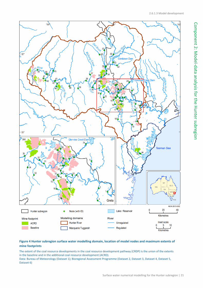
2.6.1.3 Model development
Surface water numerical modelling for the Hunter subregion | 21
Co
mp
on
ent 2
: Mo
del-d
ata analysis fo
r the
Hu
nter su
bregio
n
Figure 4 Hunter subregion surface water modelling domain, location of model nodes and maximum extents of
mine footprints
The extent of the coal resource developments in the coal resource development pathway (CRDP) is the union of the extents in the baseline and in the additional coal resource development (ACRD). Data: Bureau of Meteorology (Dataset 1); Bioregional Assessment Programme (Dataset 2, Dataset 3, Dataset 4, Dataset 5, Dataset 6)
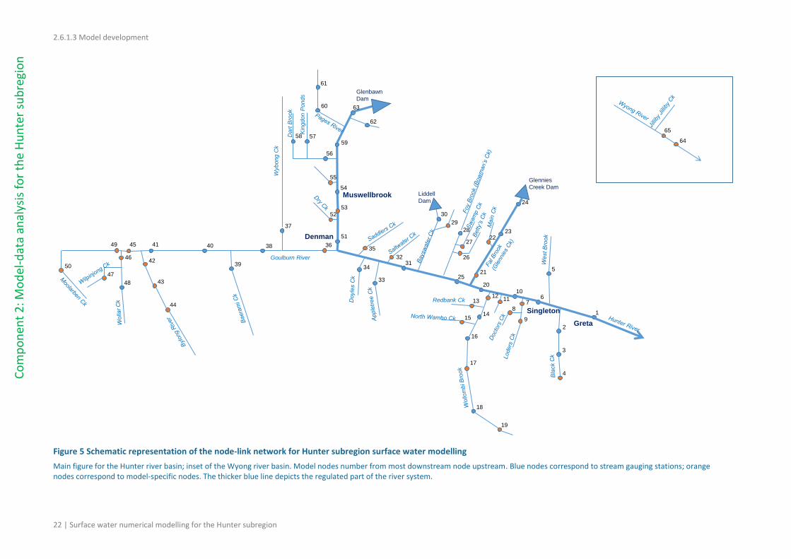
2.6.1.3 Model development
22 | Surface water numerical modelling for the Hunter subregion
Co
mp
on
ent
2: M
od
el-d
ata
anal
ysis
fo
r th
e H
un
ter
sub
regi
on
Figure 5 Schematic representation of the node-link network for Hunter subregion surface water modelling
Main figure for the Hunter river basin; inset of the Wyong river basin. Model nodes number from most downstream node upstream. Blue nodes correspond to stream gauging stations; orange nodes correspond to model-specific nodes. The thicker blue line depicts the regulated part of the river system.
Glenbawn
Dam
Glennies
Creek DamLiddell
Dam
65
64
Wybong C
k
Goulburn River
Dart
Bro
ok
Kin
gdon
Ponds
Redbank Ck44
43
42
47
48
4639
37
50
49 45 41 40 38 36
15
13
19
18
17
16
14
12
22
24
23
21
57
62
61
60
58
56
9
87
4
3
2
55
52
35
34
33
32
30
29
28
27
26
11
5
63
59
54
53
51
31
2010
6
1
25
Greta
Singleton
Denman
Muswellbrook

2.6.1.3 Model development
Surface water numerical modelling for the Hunter subregion | 23
Co
mp
on
ent 2
: Mo
del-d
ata analysis fo
r the
Hu
nter su
bregio
n
2.6.1.3.3 Choice of seasonal scaling factors for climate trend
In developing a future series of climate input, the objective is to choose the set of global climate
model (GCM) seasonal scaling factors that give the median change in mean annual precipitation in
the Hunter subregion. There are 15 available GCMs (as presented in Table 3) with seasonal scaling
factors for each of the four seasons: summer (December–February), autumn (March–May), winter
(June–August) and spring (September–November).
For each GCM the change in mean seasonal precipitation that is associated with a 1 °C global
warming is calculated. These seasonal changes are then summed to give a change in mean annual
precipitation. The resulting changes in mean annual precipitation for a 1 °C global warming in the
Hunter subregion are shown in Table 3 for each GCM. The 15 GCMs predict changes in mean
annual precipitation ranging from –6.2% (i.e. a reduction in mean annual precipitation) to 8.3%
(i.e. an increase in mean annual precipitation). The GCM with the median change is MRI (from the
Meteorological Research Institute, Japan). The corresponding projected change in mean annual
precipitation per degree of global warming is a reduction of 1.5%, or about 11 mm. The seasonal
scaling factors for MRI are +5.4%, –3.4%, –8.1% and –1.8% for summer, autumn, winter and
spring, respectively. In other words, projected increases in precipitation in the wettest season,
summer, are offset by projected decreases in the other three seasons.
Table 3 List of 15 global climate models (GCMs) and their predicted change in mean annual precipitation across the
Hunter subregion per degree of global warming
GCM Modelling group and country Change in mean annual precipitation
(%)
CCCMA T47 Canadian Climate Centre, Canada 8.3%
MIUB
Meteorological Institute of the University of Bonn, Germany
Meteorological Research Institute of the Korea Meteorological Administration, Korea
4.9%
MIROC3 Centre for Climate Research, Japan 3.7%
CCCMA T63 Canadian Climate Centre, Canada 2.7%
NCAR-PCM National Center for Atmospheric Research, USA 2.1%
NCAR-CCSM National Center for Atmospheric Research, USA 1.4%
INMCM Institute of Numerical Mathematics, Russia 0.7%
MRI Meteorological Research Institute, Japan –1.5%
CSIRO-MK3.0 CSIRO, Australia –1.6%
GFDL2.0 Geophysical Fluid, Dynamics Lab, USA –1.7%
IAP LASG/Institute of Atmospheric Physics, China –2.3%
MPI-ECHAM5 Max Planck Institute for Meteorology, German Climate Computation Centre (DKRZ), Germany
–3.1%
IPSL Institut Pierre Simon Laplace, France –4.0%
GISS-AOM NASA/Goddard Institute for Space Studies, USA –5.0%
CNRM Meteo-France, France –6.2%
Data: CSIRO (Dataset 7)

2.6.1.3 Model development
24 | Surface water numerical modelling for the Hunter subregion
Co
mp
on
ent
2: M
od
el-d
ata
anal
ysis
fo
r th
e H
un
ter
sub
regi
on
The seasonal scaling factors associated with MRI are used to generate trended precipitation inputs
for the years 2013 to 2102. The trends assume global warming of 1 °C for the period 2013 to 2042,
compared to 1983 to 2012. The global warming for 2043 to 2072 is assumed to be 1.5 °C and the
corresponding scaling factors for this period are therefore multiplied by 1.5. The global warming
for 2073 to 2102 is assumed to be 2 °C.
The scaling factors are applied to scale the daily precipitation in the climate input series that is
generated for 2013 to 2102. The resulting annual precipitation time series for the Hunter
subregion is shown in Figure 6. It depicts a cycle of 1983 to 2012 climate that is repeated a further
three times but with increasingly trended climate change scalars. It can be seen from Figure 6 that
the decrease in precipitation from 2013 to 2102 is less than the typical inter-annual variability.
Furthermore, it reduces annual precipitation rates to levels that remain much higher than were
typically encountered in the first half of the 20th century.
Figure 6 Time series of observed and projected annual precipitation averaged over the Hunter subregion
The blue line shows the time series. The red line is a centrally weighted moving average. Data: Bioregional Assessment Programme (Dataset 8)
2.6.1.3.4 Representing the hydrological changes from mining
Mine footprints
One important impact of coal mines is the interception of surface runoff that would otherwise
flow to the stream network. It is important, therefore, to determine the areas where surface
runoff will be intercepted. This area is termed the surface water footprint of the mine, and it can
differ from the groundwater footprint. For the purposes of bioregional assessments, the surface
water footprint covers the entire area disturbed by mine operations, including pits, roads, spoil

2.6.1.3 Model development
Surface water numerical modelling for the Hunter subregion | 25
Co
mp
on
ent 2
: Mo
del-d
ata analysis fo
r the
Hu
nter su
bregio
n
dumps, water storages and infrastructure. It may also include otherwise undisturbed parts of the
landscape from which natural runoff is retained in reservoirs. The footprint does not include
rehabilitated areas from which surface runoff can enter the stream network, or catchment areas
upstream of drainage channels that divert water around a mine site but do not retain it.
Mine footprint areas change over the lifetime of a mine’s operations. As new parts of the lease are
opened up for active use, the footprint increases. As mined parts of the lease are rehabilitated and
their runoff returned to natural drainage, the footprint decreases although not necessarily to pre-
mining condition. As well as the area of any final voids, the final mine footprint may also include
the area covered by any infrastructure (e.g. dams, levee banks, roads) that are intended to remain
on the site after final rehabilitation.
Time series of mine footprints for baseline and CRDP mines were compiled from spatial data
supplied by mining companies and the NSW Department of Trade and Investment, or extracted by
the Assessment team from environmental impact statements and related documents, Landsat TM
and Google Earth imagery. Details of data sources and methods used to define mine footprint time
series, including the assumptions made, are provided in Section 2.1.6 of companion product 2.1-
2.2 for the Hunter subregion (Herron et al., 2018a).
Figure 7 provides an example of temporal evolution of the mine footprint area derived for the
Ashton Coal Mine’s open-cut and underground mines. The open-cut mine is included in the
baseline and CRDP, whereas the underground mining is a baseline activity only. For modelling
purposes, it is assumed that the additional coal resource development for the open-cut mine
starts in 2018, with the maximum footprint area occurring in 2022, before reducing to a final void
area in 2035. The underground mine is assumed to commence operation in 2006 and to reach its
final extent by 2023.
Figure 7 Time series of the mine footprint area for Ashton Coal Mine’s open-cut and underground mines
The green line shows the baseline; the blue line shows the coal resource development pathway (CRDP). Data: Bioregional Assessment Programme (Dataset 9)
The full set of surface water mine footprint time series (for the 30 modelled baseline mines and 17
modelled additional coal resource developments) can be found in Section 2.1.6 of companion
product 2.1-2.2 for the Hunter subregion (Herron et al., 2018a). The maximum extents of the mine
footprints are shown in Figure 4.
Table 4 provides details of the maximum mine footprint areas for open-cut and underground for
the baseline and additional coal resource development by contributing area for each AWRA-R
model node. Node 1, which is the most downstream node in the Hunter River network, has the

2.6.1.3 Model development
26 | Surface water numerical modelling for the Hunter subregion
Co
mp
on
ent
2: M
od
el-d
ata
anal
ysis
fo
r th
e H
un
ter
sub
regi
on
largest contributing area and its mine footprint areas represent the totals from all mines upstream
of that point. Note that there can be instances where the combined maximum footprint areas of
the baseline and additional coal resource development exceed the contributing area because of
assumed changes in the timing of baseline rehabilitation due to the additional coal resource
development.
The primary ways in which coal mining affects streamflow are through interception of direct
runoff and groundwater-mediated changes in baseflow. For an open-cut mine, interception of
runoff is assumed to occur in the area covered by the mine’s surface water footprint. Within this
area, 100% of the streamflow that would have been generated in the absence of the mine is
assumed to be retained on site and does not contribute to predicted streamflow.
For an underground mine, surface subsidence associated with the collapse of the longwall panels
is expected to lead to increased ponding at the surface. This increased ponding is likely to result in
a decrease in natural flow to the streams. A 5% reduction in runoff in areas covered by an
underground mine footprint is conservatively (i.e. impact is likely to be smaller) assumed, which
factors in regulatory requirements on mining companies to minimise the impacts from mine
subsidence through such steps as appropriate longwall orientation and drainage management.
The hydrological change to baseflow is estimated using the groundwater model, which is
described in detail in Section 2.6.2.3 of companion product 2.6.2 for the Hunter subregion (Herron
et al., 2018b). The groundwater model estimates monthly baseflow for each surface water model
node under the baseline and CRDP. The difference between CRDP and baseline simulations is
taken as the monthly hydrological change in baseflow, and is then equally partitioned to obtain
the daily changes.
Additional coal resource developments that were not modelled due to insufficient data (see
Section 2.3.4 of companion product 2.3 for the Hunter subregion (Dawes et al., 2018)) are
considered further in the impact and risk analysis (see companion product 3-4 for the Hunter
subregion, as listed in Table 2).
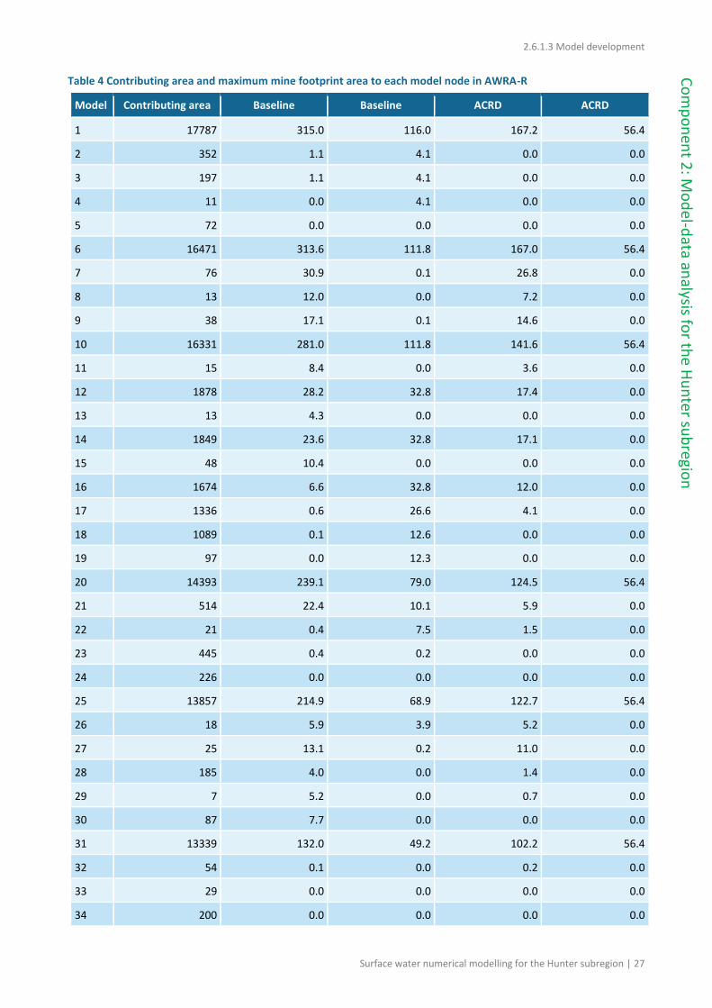
2.6.1.3 Model development
Surface water numerical modelling for the Hunter subregion | 27
Co
mp
on
ent 2
: Mo
del-d
ata analysis fo
r the
Hu
nter su
bregio
n
Table 4 Contributing area and maximum mine footprint area to each model node in AWRA-R
Model node
Contributing area
(km2)
Baseline
Open-cut
maximum footprint
(km2)
Baseline
Underground
maximum footprint
(km2)
ACRD
Open-cut
maximum footprint
(km2)
ACRD
Underground
maximum footprint
(km2)
1 17787 315.0 116.0 167.2 56.4
2 352 1.1 4.1 0.0 0.0
3 197 1.1 4.1 0.0 0.0
4 11 0.0 4.1 0.0 0.0
5 72 0.0 0.0 0.0 0.0
6 16471 313.6 111.8 167.0 56.4
7 76 30.9 0.1 26.8 0.0
8 13 12.0 0.0 7.2 0.0
9 38 17.1 0.1 14.6 0.0
10 16331 281.0 111.8 141.6 56.4
11 15 8.4 0.0 3.6 0.0
12 1878 28.2 32.8 17.4 0.0
13 13 4.3 0.0 0.0 0.0
14 1849 23.6 32.8 17.1 0.0
15 48 10.4 0.0 0.0 0.0
16 1674 6.6 32.8 12.0 0.0
17 1336 0.6 26.6 4.1 0.0
18 1089 0.1 12.6 0.0 0.0
19 97 0.0 12.3 0.0 0.0
20 14393 239.1 79.0 124.5 56.4
21 514 22.4 10.1 5.9 0.0
22 21 0.4 7.5 1.5 0.0
23 445 0.4 0.2 0.0 0.0
24 226 0.0 0.0 0.0 0.0
25 13857 214.9 68.9 122.7 56.4
26 18 5.9 3.9 5.2 0.0
27 25 13.1 0.2 11.0 0.0
28 185 4.0 0.0 1.4 0.0
29 7 5.2 0.0 0.7 0.0
30 87 7.7 0.0 0.0 0.0
31 13339 132.0 49.2 102.2 56.4
32 54 0.1 0.0 0.2 0.0
33 29 0.0 0.0 0.0 0.0
34 200 0.0 0.0 0.0 0.0
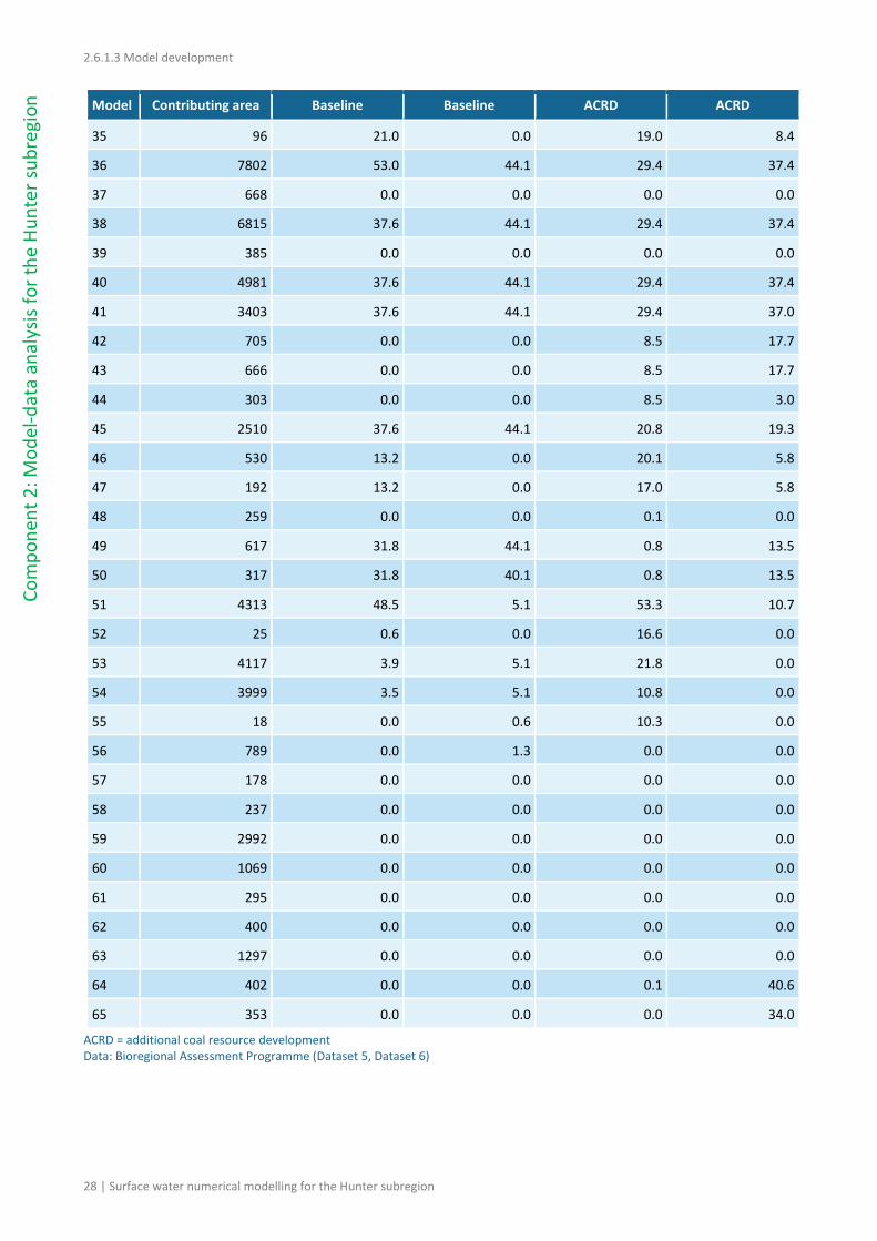
2.6.1.3 Model development
28 | Surface water numerical modelling for the Hunter subregion
Co
mp
on
ent
2: M
od
el-d
ata
anal
ysis
fo
r th
e H
un
ter
sub
regi
on
Model node
Contributing area
(km2)
Baseline
Open-cut
maximum footprint
(km2)
Baseline
Underground
maximum footprint
(km2)
ACRD
Open-cut
maximum footprint
(km2)
ACRD
Underground
maximum footprint
(km2)
35 96 21.0 0.0 19.0 8.4
36 7802 53.0 44.1 29.4 37.4
37 668 0.0 0.0 0.0 0.0
38 6815 37.6 44.1 29.4 37.4
39 385 0.0 0.0 0.0 0.0
40 4981 37.6 44.1 29.4 37.4
41 3403 37.6 44.1 29.4 37.0
42 705 0.0 0.0 8.5 17.7
43 666 0.0 0.0 8.5 17.7
44 303 0.0 0.0 8.5 3.0
45 2510 37.6 44.1 20.8 19.3
46 530 13.2 0.0 20.1 5.8
47 192 13.2 0.0 17.0 5.8
48 259 0.0 0.0 0.1 0.0
49 617 31.8 44.1 0.8 13.5
50 317 31.8 40.1 0.8 13.5
51 4313 48.5 5.1 53.3 10.7
52 25 0.6 0.0 16.6 0.0
53 4117 3.9 5.1 21.8 0.0
54 3999 3.5 5.1 10.8 0.0
55 18 0.0 0.6 10.3 0.0
56 789 0.0 1.3 0.0 0.0
57 178 0.0 0.0 0.0 0.0
58 237 0.0 0.0 0.0 0.0
59 2992 0.0 0.0 0.0 0.0
60 1069 0.0 0.0 0.0 0.0
61 295 0.0 0.0 0.0 0.0
62 400 0.0 0.0 0.0 0.0
63 1297 0.0 0.0 0.0 0.0
64 402 0.0 0.0 0.1 40.6
65 353 0.0 0.0 0.0 34.0
ACRD = additional coal resource development Data: Bioregional Assessment Programme (Dataset 5, Dataset 6)
2.6.1.3 Model development
Surface water numerical modelling for the Hunter subregion | 29
Co
mp
on
ent 2
: Mo
del-d
ata analysis fo
r the
Hu
nter su
bregio
n
2.6.1.3.5 Modelling river management
The river model, AWRA-R, is used to simulate some aspects of the management and regulation of
the Hunter River, but this is undertaken differently to the Hunter Integrated Quantity-Quality
Model (IQQM) (Simons et al., 1996), used by state agencies to set and assess river management
rules, water sharing plans and allocations. This reflects the different purposes for which these
models have been developed. The implementation of AWRA-R in the bioregional assessment for
the Hunter subregion was not specifically developed for river operations planning and
management and, without further development, should not be used for this purpose.
The Hunter River is regulated by two major dams, Glenbawn Dam (capacity of 750,000 GL) and
Glennies Creek Dam (283,000 GL) (Figure 4). These dams supply water to downstream irrigation,
industry and town water. Basic characteristics controlling the operations of these dams (e.g. dead
volume, surface area and the split values for releases to various types of water user) are taken
from IQQM inputs. Other variables required for AWRA-R are largely based on existing
management rules.
2.6.1.3.6 Rules to simulate industry water discharge
A simple set of rules to simulate industry water discharge within the Hunter River Salinity Trading
Scheme (HRSTS) was developed based on the analysis reported in Section 2.1.4 in companion
product 2.1-2.2 for the Hunter subregion (Herron et al., 2018a). The resulting rules are not
intended to replicate the operations of HRSTS, which is a real-time scheme contingent upon
human decision making. Instead, the summary rules were developed that describe the gross
characteristics of the scheme and are amenable to prospective (i.e. future) modelling.
Discharges under HRSTS are simulated when modelled streamflow exceeds the prescribed
thresholds at three locations along the Hunter River. Discharge amounts at these locations are
modelled as functions of the mean annual HRSTS discharges and the rate of discharge as a
function of streamflow volume in exceedance of the thresholds. Both these variables were
obtained from analysis of historical releases. Any modelled discharges are assumed to be
distributed from all mines upstream of the three reaches.
References
Dawes WR, Herron NF, Macfarlane C, Rachakonda PK, Henderson BL, Ford JH, Wilkes PG,
Marvanek SP, Ramage A (2018) Conceptual modelling for the Hunter subregion. Product 2.3
for the Hunter subregion from the Northern Sydney Basin Bioregional Assessment.
Department of the Environment and Energy, Bureau of Meteorology, CSIRO and Geoscience
Australia, Australia. http://data.bioregionalassessments.gov.au/product/NSB/HUN/2.3.
Herron NF, Frery E, Crosbie R, Peña-Arancibia J, Zhang YQ, Viney N, Rachakonda PK, Ramage A,
Marvanek SP, Gresham M, McVicar TR, Wilkins A (2018a) Observations analysis, statistical
analysis and interpolation for the Hunter subregion. Product 2.1-2.2 for the Hunter
subregion from the Northern Sydney Basin Bioregional Assessment. Department of the
Environment and Energy, Bureau of Meteorology, CSIRO and Geoscience Australia, Australia.
http://data.bioregionalassessments.gov.au/product/NSB/HUN/2.1-2.2.

2.6.1.3 Model development
30 | Surface water numerical modelling for the Hunter subregion
Co
mp
on
ent
2: M
od
el-d
ata
anal
ysis
fo
r th
e H
un
ter
sub
regi
on
Herron NF, Peeters L, Crosbie R, Marvanek SP, Pagendam D, Ramage A, Rachakonda PK and
Wilkins A (2018b) Groundwater numerical modelling for the Hunter subregion. Product 2.6.2
for the Hunter subregion from the Northern Sydney Basin Bioregional Assessment.
Department of the Environment and Energy, Bureau of Meteorology, CSIRO and Geoscience
Australia, Australia. http://data.bioregionalassessments.gov.au/product/NSB/HUN/2.6.2.
Simons M, Podger G and Cooke R (1996) IQQM – a hydrologic modelling tool for water resource
and salinity management. Environmental Software 11, 185–192. DOI: 10.1016/s0266-
9838(96)00019-6.
Viney N (2016) Surface water modelling. Submethodology M06 from the Bioregional Assessment
Technical Programme. Department of the Environment and Energy, Bureau of Meteorology,
CSIRO and Geoscience Australia, Australia.
http://data.bioregionalassessments.gov.au/submethodology/M06.
Datasets
Dataset 1 Bureau of Meteorology (2011) Geofabric surface cartography, v2.1. Bioregional
Assessment Source Dataset. Viewed 21 April 2015,
http://data.bioregionalassessments.gov.au/dataset/5342c4ba-f094-4ac5-a65d-
071ff5c642bc.
Dataset 2 Bioregional Assessment Programme (2014) Selected streamflow gauges within and near
the Hunter subregion. Bioregional Assessment Derived Dataset. Viewed 02 March 2016,
http://data.bioregionalassessments.gov.au/dataset/e83b0500-6254-47e1-b103-
5e6b5961fe6f.
Dataset 3 Bioregional Assessment Programme (2016) HUN AWRA-L Calibration Catchments v01.
Bioregional Assessment Derived Dataset. Viewed 21 July 2016,
http://data.bioregionalassessments.gov.au/dataset/c60e96db-f2a2-4036-9a2e-
353de289a715.
Dataset 4 Bioregional Assessment Programme (2016) HUN AWRA-R calibration nodes v01.
Bioregional Assessment Derived Dataset. Viewed 18 July 2016,
http://data.bioregionalassessments.gov.au/dataset/f2da394a-3d08-4cf4-8c24-
bf7751ea06a1.
Dataset 5 Bioregional Assessment Programme (2016) HUN AWRA-R calibration catchments v01.
Bioregional Assessment Derived Dataset. Viewed 17 February 2016,
http://data.bioregionalassessments.gov.au/dataset/d419aae0-1cb3-48a8-82de-
941398a80e3a.
Dataset 6 Bioregional Assessment Programme (2016) HUN SW modelling total mine footprint v01.
Bioregional Assessment Derived Dataset. Viewed 31 August 2016,
http://data.bioregionalassessments.gov.au/dataset/b78597ba-4781-4b95-80c3-
d6c11cb2e595.
2.6.1.3 Model development
Surface water numerical modelling for the Hunter subregion | 31
Co
mp
on
ent 2
: Mo
del-d
ata analysis fo
r the
Hu
nter su
bregio
n
Dataset 7 CSIRO (2016) SEACI GCM Scaling. Bioregional Assessment Source Dataset. Viewed 03
February 2017, http://data.bioregionalassessments.gov.au/dataset/bde1e7b7-5bb3-483c-
8616-c4176fde8818
Dataset 8 Bioregional Assessment Programme (2016) HUN Future climate rainfall v01. Bioregional
Assessment Derived Dataset. Viewed 23 November 2016,
http://data.bioregionalassessments.gov.au/dataset/4e4420e8-7d42-43bc-a63d-
6ca3f07d8036.
Dataset 9 Bioregional Assessment Programme (2016) HUN Mine footprints for timeseries.
Bioregional Assessment Derived Dataset. Viewed 04 March 2016,
http://data.bioregionalassessments.gov.au/dataset/1e18f597-c8dd-4dae-b460-
de9f5ebb1c6a.

2.6.1.3 Model development
32 | Surface water numerical modelling for the Hunter subregion
Co
mp
on
ent
2: M
od
el-d
ata
anal
ysis
fo
r th
e H
un
ter
sub
regi
on

2.6.1.4 Calibration
Surface water numerical modelling for the Hunter subregion | 33
Co
mp
on
ent 2
: Mo
del-d
ata analysis fo
r the
Hu
nter su
bregio
n
2.6.1.4 Calibration
Summary
This section describes the calibration of the two components of surface water modelling in
the Hunter subregion. These components are the Australian Water Resources Assessment
(AWRA) landscape model (AWRA-L), and the AWRA river model (AWRA-R).
AWRA-L is regionally calibrated at 14 unregulated catchments using two calibration schemes:
one biased towards high streamflow, and another biased towards low streamflow. The two
parameter sets obtained from the two model calibrations are used to guide the generation of
the 3000 parameter sets used for the uncertainty analysis (Section 2.6.1.5) and predictions
(Section 2.6.1.6). The high-streamflow and low-streamflow calibrations perform reasonably
well for predicting daily runoff for a wide range of streamflow conditions. For the nine
hydrological response variables predicted by the model (Section 2.6.1.6), the high-streamflow
calibration outperforms the low-streamflow calibration for predicting annual flow (AF) only.
The low-streamflow calibration provides better predictions for the other eight hydrological
response variables. Both calibrations noticeably over estimate high-flow days (FD) and
interquartile range (IQR), but under estimate zero-flow days (ZFD), low-flow days (LFD), low-
flow spells (LFS) and length of the longest low-flow spell (LLFS).
AWRA-R is calibrated for 20 streamflow gauging sites of the Hunter River and tributaries.
Using runoff from both AWRA-L calibrations, two concurrent AWRA-R calibrations are
conducted: a high-streamflow calibration and a low-streamflow calibration. Both variants
perform well overall, with the high-streamflow calibration outperforming the low-streamflow
calibration. However, the low-streamflow calibration is markedly better than the high-
streamflow calibration for six out of nine hydrological response variables (including all low-
streamflow metrics); and marginally worse for IQR, FD and daily streamflow at the 99th
percentile (P99).
This section also assesses the AWRA-R model components representing river management
(including water resources assessment and allocations, dam storage volumes and dam
releases) that were calibrated using simulated or modelled outputs (Section 2.6.1.3). Results
show that these components of the model capture relevant aspects of river management for
a wide range of climate conditions.
2.6.1.4.1 Australian Water Resources Assessment landscape model
Data
Data needed for calibration of the Australian Water Resources Assessment (AWRA) landscape
model (AWRA-L) include climate data and streamflow. The calibration period used for AWRA-L
model development was from 1983 to 2012, which includes both wet and dry periods.
The landscape water balance model AWRA-L is run using gridded data of maximum temperature,
minimum temperature, incoming solar radiation and precipitation. Daily grids (cell resolution of
0.05 x 0.05 degrees; ~5 x 5 km) of these variables are generated for the Australian continent by
2.6.1.4 Calibration
34 | Surface water numerical modelling for the Hunter subregion
Co
mp
on
ent
2: M
od
el-d
ata
anal
ysis
fo
r th
e H
un
ter
sub
regi
on
the Bureau of Meteorology (Dataset 1). Details of this dataset are provided in Section 2.1.1 of
companion product 2.1-2.2 for the Hunter subregion (Herron et al., 2018).
Daily stage and streamflow data from 14 streamflow gauging stations with unregulated
catchments located in and near the Hunter subregion were used to calibrate AWRA-L. These
gauging stations and the catchments subtended by them are shown in Figure 8. Ten stations are
located in the Hunter river basin and four in the Macquarie-Tuggerah lakes basin. Of the 14
stations, ten are located within the modelling domain (Section 2.6.1.3) and four are located very
close by. Site details are summarised in Section 2.1.4 of companion product 2.1-2.2 for the Hunter
subregion (Herron et al., 2018). Observed daily mean streamflow data for the above gauges for
1983 to 2012 were derived from NSW DPI water data supplied by the Bureau of Meteorology
(Dataset 2).
Criteria for selecting the calibration catchments include that they:
have catchment areas greater than 50 km2
have long-term measurements (more than 20 years from 1983)
are currently not impacted by coal mining or coal seam gas extraction or other major
extractive industries
have no significant flow regulation (e.g. dams)
are not nested (i.e. not directly upstream or downstream of another selected gauge)
are located within or close to the Hunter subregion and have similar catchment sizes and
climate regimes.
Catchment boundaries for the 14 calibration catchments were delineated using the Australian
Hydrological Geospatial Fabric (Geofabric) (Bureau of Meteorology, Dataset 5).

2.6.1.4 Calibration
Surface water numerical modelling for the Hunter subregion | 35
Co
mp
on
ent 2
: Mo
del-d
ata analysis fo
r the
Hu
nter su
bregio
n
Figure 8 The 14 streamflow gauging stations used for AWRA-L model calibration and their contributing areas
AWRA-L = Australian Water Resources Assessment landscape model Data: Bioregional Assessment Programme (Dataset 3, Dataset 4), Bureau of Meteorology (Dataset 5)

2.6.1.4 Calibration
36 | Surface water numerical modelling for the Hunter subregion
Co
mp
on
ent
2: M
od
el-d
ata
anal
ysis
fo
r th
e H
un
ter
sub
regi
on
Calibration evaluation metrics
As per companion submethodology M06 (as listed in Table 1) for surface water modelling (Viney,
2016), two regional model calibrations were undertaken: one biased towards predicting high-
streamflow behaviour; the second biased towards predicting low-streamflow behaviour. Three
metrics were used to evaluate model performance:
Daily efficiency (Ed), also referred to as the Nash–Sutcliffe efficiency, which compares daily
model predictions against daily observation data. Efficiency values range from 1 (which
indicates perfect agreement between prediction and observation) to minus infinity.
Model bias (B), the prediction error divided by the sum of observations, which gives an
indication of the model’s overall tendency towards underprediction or overprediction. Bias
ranges from –1 (negative values indicate underprediction) to plus infinity (overprediction).
The closer the model bias is to zero, the better the model is at estimating the observed
volume of streamflow.
F value, which seeks to combine efficiency and bias into a single metric. The high-streamflow
calibration uses a version of F given by F1 = (Ed(1.0) + Em)/2 – 5|ln(1 + B)|2.5, where Ed(1.0) is
the efficiency of daily streamflow (without transformation, or with a Box-Cox lambda value
of 1.0) (Box and Cox, 1964), Em is the efficiency of the monthly predictions assessed against
monthly observations, and B is the bias. The low-streamflow calibration uses a version of F
given by F2 = Ed(0.1) – 5|ln(1 + B)|2.5, where Ed(0.1) is the efficiency of daily streamflow
transformed with a Box-Cox lambda value of 0.1.
Model calibration results
Figure 9 and Table 5 summarise results of the two model calibrations for the 14 calibration
catchments in terms of the three performance metrics. The parameter values for the two
calibrations are included in Bioregional Assessment Programme (Dataset 6). The high-streamflow
calibration yields a reasonable Nash–Sutcliffe efficiency of daily streamflow, indicated by a median
Ed(1.0) of 0.45 and interquartile range of 0.4 to 0.6. Overall model bias is low with a median bias of
–0.03, but the interquartile range indicates variability across the 14 catchments with considerable
overestimation in some catchments. The high-streamflow calibration yields a median F1 of 0.37,
which is only 0.08 less than the median Ed(1.0), indicating overall low model bias. The Ed(1.0) value
is negative (suggesting poor simulation) for one catchment: –0.16 at gauging station 211010 on
the Wyong River, with a prediction bias of 0.68.
The low-streamflow calibration is evaluated against the daily streamflow data transformed with a
Box-Cox lambda value of 0.1. The low-streamflow calibration yields similar efficiency to the high-
streamflow calibration, indicated by a median Ed(1.0) of 0.41. The Ed(1.0) is greater than 0.34 for
11 of the 14 catchments and remains above zero for all catchments. The median bias of –0.12
indicates an overall tendency for underprediction by the low-streamflow calibration.
The performance of the high-streamflow calibration for the 14 catchments is not significantly
related to catchment wetness, as it does not perform better or worse with a wetter climate. The
Ed(0.1) values of the low-streamflow calibration are moderately correlated with catchment

2.6.1.4 Calibration
Surface water numerical modelling for the Hunter subregion | 37
Co
mp
on
ent 2
: Mo
del-d
ata analysis fo
r the
Hu
nter su
bregio
n
wetness (r2 = 0.51, p < 0.01), but the statistical significance of this correlation does not extend
to F2.
The 14 calibration catchments cover a wide range of climate and topographic conditions, with
mean annual flow (AF) ranging from 33 mm/year at catchment 210040 (Wybong Creek) to
425 mm/year at catchment 210011 (Williams River) (Table 5). This suggests that AWRA-L can
predict streamflow variability reasonably in the Hunter subregion where climate conditions vary
widely.
Figure 9 Summary of two AWRA-L model calibrations for the Hunter subregion
AWRA-L = Australian Water Resources Assessment landscape model In each boxplot, the bottom, middle and top of the box are the 25th, 50th and 75th percentiles, and the bottom and top whiskers are the 10th and 90th percentiles. F1 is the F value for high-streamflow calibration; F2 is the F value for the low-streamflow calibration; Ed(1.0) is the daily efficiency with a Box-Cox lambda value of 1.0; Ed(0.1) is the daily efficiency with a Box-Cox lambda value of 0.1; B is model bias. Data: Bioregional Assessment Programme (Dataset 6)
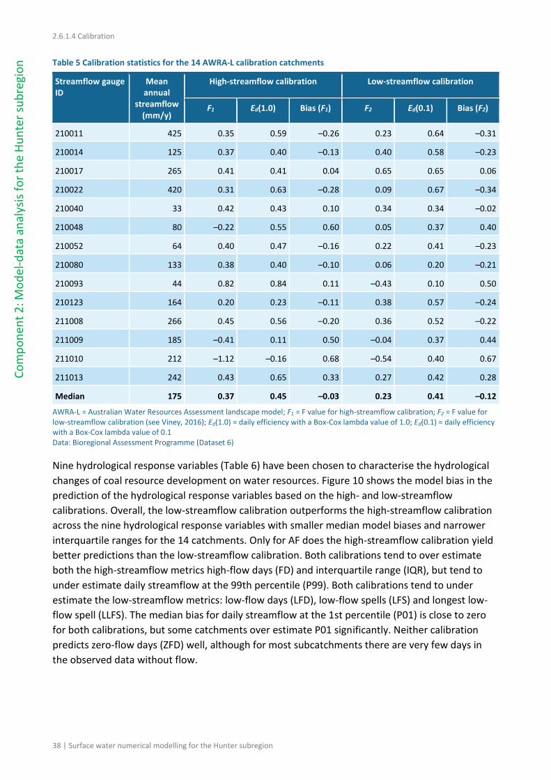
2.6.1.4 Calibration
38 | Surface water numerical modelling for the Hunter subregion
Co
mp
on
ent
2: M
od
el-d
ata
anal
ysis
fo
r th
e H
un
ter
sub
regi
on
Table 5 Calibration statistics for the 14 AWRA-L calibration catchments
Streamflow gauge ID
Mean annual
streamflow (mm/y)
High-streamflow calibration Low-streamflow calibration
F1 Ed(1.0) Bias (F1) F2 Ed(0.1) Bias (F2)
210011 425 0.35 0.59 –0.26 0.23 0.64 –0.31
210014 125 0.37 0.40 –0.13 0.40 0.58 –0.23
210017 265 0.41 0.41 0.04 0.65 0.65 0.06
210022 420 0.31 0.63 –0.28 0.09 0.67 –0.34
210040 33 0.42 0.43 0.10 0.34 0.34 –0.02
210048 80 –0.22 0.55 0.60 0.05 0.37 0.40
210052 64 0.40 0.47 –0.16 0.22 0.41 –0.23
210080 133 0.38 0.40 –0.10 0.06 0.20 –0.21
210093 44 0.82 0.84 0.11 –0.43 0.10 0.50
210123 164 0.20 0.23 –0.11 0.38 0.57 –0.24
211008 266 0.45 0.56 –0.20 0.36 0.52 –0.22
211009 185 –0.41 0.11 0.50 –0.04 0.37 0.44
211010 212 –1.12 –0.16 0.68 –0.54 0.40 0.67
211013 242 0.43 0.65 0.33 0.27 0.42 0.28
Median 175 0.37 0.45 –0.03 0.23 0.41 –0.12
AWRA-L = Australian Water Resources Assessment landscape model; F1 = F value for high-streamflow calibration; F2 = F value for low-streamflow calibration (see Viney, 2016); Ed(1.0) = daily efficiency with a Box-Cox lambda value of 1.0; Ed(0.1) = daily efficiency with a Box-Cox lambda value of 0.1 Data: Bioregional Assessment Programme (Dataset 6)
Nine hydrological response variables (Table 6) have been chosen to characterise the hydrological
changes of coal resource development on water resources. Figure 10 shows the model bias in the
prediction of the hydrological response variables based on the high- and low-streamflow
calibrations. Overall, the low-streamflow calibration outperforms the high-streamflow calibration
across the nine hydrological response variables with smaller median model biases and narrower
interquartile ranges for the 14 catchments. Only for AF does the high-streamflow calibration yield
better predictions than the low-streamflow calibration. Both calibrations tend to over estimate
both the high-streamflow metrics high-flow days (FD) and interquartile range (IQR), but tend to
under estimate daily streamflow at the 99th percentile (P99). Both calibrations tend to under
estimate the low-streamflow metrics: low-flow days (LFD), low-flow spells (LFS) and longest low-
flow spell (LLFS). The median bias for daily streamflow at the 1st percentile (P01) is close to zero
for both calibrations, but some catchments over estimate P01 significantly. Neither calibration
predicts zero-flow days (ZFD) well, although for most subcatchments there are very few days in
the observed data without flow.
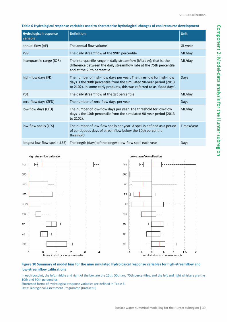
2.6.1.4 Calibration
Surface water numerical modelling for the Hunter subregion | 39
Co
mp
on
ent 2
: Mo
del-d
ata analysis fo
r the
Hu
nter su
bregio
n
Table 6 Hydrological response variables used to characterise hydrological changes of coal resource development
Hydrological response variable
Definition Unit
annual flow (AF) The annual flow volume GL/year
P99 The daily streamflow at the 99th percentile ML/day
interquartile range (IQR) The interquartile range in daily streamflow (ML/day); that is, the difference between the daily streamflow rate at the 75th percentile and at the 25th percentile
ML/day
high-flow days (FD) The number of high-flow days per year. The threshold for high-flow days is the 90th percentile from the simulated 90-year period (2013 to 2102). In some early products, this was referred to as ‘flood days’.
Days
P01 The daily streamflow at the 1st percentile ML/day
zero-flow days (ZFD) The number of zero-flow days per year Days
low-flow days (LFD) The number of low-flow days per year. The threshold for low-flow days is the 10th percentile from the simulated 90-year period (2013 to 2102).
ML/day
low-flow spells (LFS) The number of low-flow spells per year. A spell is defined as a period of contiguous days of streamflow below the 10th percentile threshold.
Times/year
longest low-flow spell (LLFS) The length (days) of the longest low-flow spell each year Days
Figure 10 Summary of model bias for the nine simulated hydrological response variables for high-streamflow and
low-streamflow calibrations
In each boxplot, the left, middle and right of the box are the 25th, 50th and 75th percentiles, and the left and right whiskers are the 10th and 90th percentiles. Shortened forms of hydrological response variables are defined in Table 6. Data: Bioregional Assessment Programme (Dataset 6)

2.6.1.4 Calibration
40 | Surface water numerical modelling for the Hunter subregion
Co
mp
on
ent
2: M
od
el-d
ata
anal
ysis
fo
r th
e H
un
ter
sub
regi
on
It is noted that the parameter sets obtained from the regional model calibrations are not applied
directly to the uncertainty analysis (Section 2.6.1.5). However, they are taken as reference values
to evaluate performance of the best 10% of parameter sets (i.e. 300 model runs) selected for each
hydrological response variable.
Implications for model predictions
Results from the regional model calibrations (Table 5 and Figure 9) suggest that AWRA-L performs
reasonably well in estimating high streamflow and low streamflow in the Hunter subregion.
It is noted that when the model is calibrated against observations from 14 streamflow gauges it
does not generate a uniform model performance. Though the model performs well overall, it
performs poorly in some catchments and does not estimate the suite of hydrological response
variables equally effectively. For instance, the high-streamflow model calibration generates a poor
model performance at gauge 211010. The model noticeably under estimates streamflow for
gauges 211010 and 210048. For other gauges in the Hunter subregion, AWRA-L performs well in
terms of model efficiency and bias.
As opposed to model calibration against observation at each individual catchment, a key
characteristic of regional model calibration against observations from multiple catchments is that
there is no noticeable degradation from model calibration to model prediction (Viney et al., 2014).
For both the high- and low-streamflow calibrations, the biases at the majority of individual stream
gauging sites are in the range –20% to +40%. Given the regionalisation methodology applied here,
it is reasonable to assume that prediction biases in ungauged parts of the subregion will be similar.
This provides confidence when applying AWRA-L to each model node where there are no
streamflow observations.
The results from the simulated hydrological response variables (Figure 10) show that in the Hunter
subregion, AWRA-L calibrated against high daily streamflow is not always better for estimating the
high-streamflow hydrological response variables; and the model calibrated against low daily
streamflow performs consistently better than that based on the high-streamflow calibration for
estimating most hydrological response variables. Both calibrations, however, show large
uncertainty in predicting some of the hydrological response variables. In general, one or other of
the two calibration sets provides predictions of the hydrological response variables with little bias.
An exception is for the variable describing the number of low-flow days, which both parameter
sets severely under-predict. This suggests that less confidence may be ascribed to the prediction
of this variable in Section 2.6.1.6 than to the prediction of the other variables. Using both
calibration parameter sets to generate the 3000 parameter sets for the simulations is expected to
provide a reasonable estimate of uncertainty for each hydrological response variable.
2.6.1.4.2 Australian Water Resources Assessment river model
Data
Input data to drive the AWRA river model (AWRA-R) calibration include climate, potential
evaporation, catchment runoff (from AWRA-L), groundwater depth, and power generation and
town water supply diversions. Calibration datasets against which performance of AWRA-R and the

2.6.1.4 Calibration
Surface water numerical modelling for the Hunter subregion | 41
Co
mp
on
ent 2
: Mo
del-d
ata analysis fo
r the
Hu
nter su
bregio
n
various modules were evaluated are daily streamflow, dam storage volumes, water allocations,
dam releases and irrigation diversions.
The calibration period for the different AWRA-R components generally covered 1981 to 2012.
However, some calibration datasets did not cover this entire period and suitable periods were
chosen based on data availability; details of these datasets are provided below.
The only direct climate input into AWRA-R is daily precipitation, which is used to calculate
precipitation directly on the river channel and storages. Daily gridded precipitation data from the
Bureau of Meteorology (Dataset 1) have been used in the calibration of AWRA-R. The gridded data
were clipped and aggregated (spatially averaged) using reach subcatchment boundaries defined in
the Hunter river system AWRA-R node-link network (Bioregional Assessment Programme, Dataset
7 and Dataset 8).
Daily estimates of potential evaporation and catchment runoff were obtained from the calibrated
AWRA-L simulation (Bioregional Assessment Programme, Dataset 6) and aggregated to the reach
scale defined by the Hunter river system node-link network (Bioregional Assessment Programme,
Dataset 7 and Dataset 8) for input into AWRA-R.
Industry diversions (including those for power stations and town water supply) are not calibrated
and are used as inputs in AWRA-R (NSW Office of Water, Dataset 9).
The AWRA-R model used for calibration comprises 52 nodes and their contributing areas, shown in
Figure 11. These include the 34 gauging stations for which stage and streamflow data were
obtained for model calibration (Bureau of Meteorology, Dataset 5). Twenty of the gauging stations
are non-headwater gauges: they include 11 on the Hunter River, three on each of Wollombi Brook
and the Goulburn River and three on other Hunter River tributaries (red triangles in Figure 11). The
other 32 calibration model nodes (black dots in Figure 11) comprise the 14 gauging stations on
headwater streams, plus 18 of the 29 model nodes (see Section 2.6.1.3.2), located on ungauged
headwater streams. Daily streamflows at the 18 ungauged nodes are simulated by AWRA-L
(Bioregional Assessment Programme, Dataset 6) and stages obtained from idealised cross-sections
at each location (see companion product 2.1-2.2 for the Hunter subregion (Herron et al., 2018);
Bioregional Assessment Programme, Dataset 10). Eleven model nodes, located on ungauged
reaches downstream of other model nodes, are not used in the calibration but are needed for the
AWRA-R model simulations.
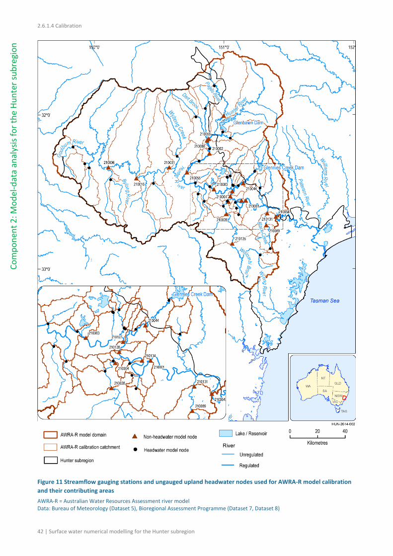
2.6.1.4 Calibration
42 | Surface water numerical modelling for the Hunter subregion
Co
mp
on
ent
2: M
od
el-d
ata
anal
ysis
fo
r th
e H
un
ter
sub
regi
on
Figure 11 Streamflow gauging stations and ungauged upland headwater nodes used for AWRA-R model calibration
and their contributing areas
AWRA-R = Australian Water Resources Assessment river model Data: Bureau of Meteorology (Dataset 5), Bioregional Assessment Programme (Dataset 7, Dataset 8)

2.6.1.4 Calibration
Surface water numerical modelling for the Hunter subregion | 43
Co
mp
on
ent 2
: Mo
del-d
ata analysis fo
r the
Hu
nter su
bregio
n
Daily irrigation and mining diversions were sourced from the Hunter Integrated Quantity-Quality
Model (IQQM) (NSW Office of Water, Dataset 9), aggregated to monthly for the period 1981 to
2012. Irrigation diversions were used to calibrate the AWRA-R irrigation and dam storage and
releases modules. Mining diversions were used as inputs in the calibration. Since mining diversions
have similar seasonal patterns to irrigation diversions, the AWRA-R irrigation module is used to
simulate mining diversions under baseline and CRDP.
Available observed stored volumes as well as allocations (NSW Office of Water, Dataset 9) were
used in preference to simulated data for calibration of the dam storage module. These data were
available from 1993 to 2012.
Daily dam releases (for Glenbawn Dam and Glennies Creek Dam) were sourced from the Hunter
IQQM (NSW Office of Water, Dataset 9). These data were available from 1981 to 2012.
All data used for calibration of allocation, dam storage and dam releases overlapped the period
from 1993 to 2012, hence this period was chosen for calibration of these components.
Model calibration results
Streamflow routing and reach water balance
AWRA-R was calibrated using 34 streamflow gauges defining a concurrent number of modelling
reaches. Two variants of the model were calibrated using AWRA-L high-streamflow and low-
streamflow calibration outputs, respectively (Bioregional Assessment Programme, Dataset 6).
Eight of the 11 AWRA-R parameters (Viney, 2016) were calibrated; one routing parameter was
fixed and the floodplain module (two parameters) was not implemented. The parameter values
for the two calibrations are included in Bioregional Assessment Programme (Dataset 6).
The agreement of both high- and low-streamflow AWRA-R calibrations were assessed using the
daily Nash–Sutcliffe efficiency (Ed) for daily streamflow (Ed(1.0)) and for daily streamflow
transformed with a Box-Cox lambda value of 0.1 (Ed(0.1)) as well as both F1 and F2 values (see
Section 2.6.1.4.1). The bias generally remains very low as each reach is individually calibrated and
parameterised, as opposed to the regional calibration implemented for AWRA-L (see companion
submethodology M06 (as listed in Table 1) for surface water modelling (Viney, 2016)).
The performance is reported for the 20 non-headwater gauges depicted as triangles in Figure 11
and where routing and reach water balance processes (including runoff from catchments between
the two nodes, river water diversions, groundwater fluxes and overbank flow) take place.
Figure 12 shows boxplots summarising the performance of the AWRA-R high-streamflow and
AWRA-R low-streamflow calibrations in the 20 gauges. Table 7 presents a summary of the
goodness-of-fit metrics used to evaluate the two model variants. In terms of Ed(1.0) (emphasis on
high flows), the AWRA-R high-streamflow calibration agrees reasonably well with observations,
indicated by a median Ed(1.0) of 0.73 (interquartile range of 0.53 to 0.79) and a median bias of
0.005. Thirteen of the 20 reaches have an Ed(1.0) greater than 0.6, whereas only reach 210006
(Goulburn River at Coggan) has an Ed(1.0) less than 0.25.
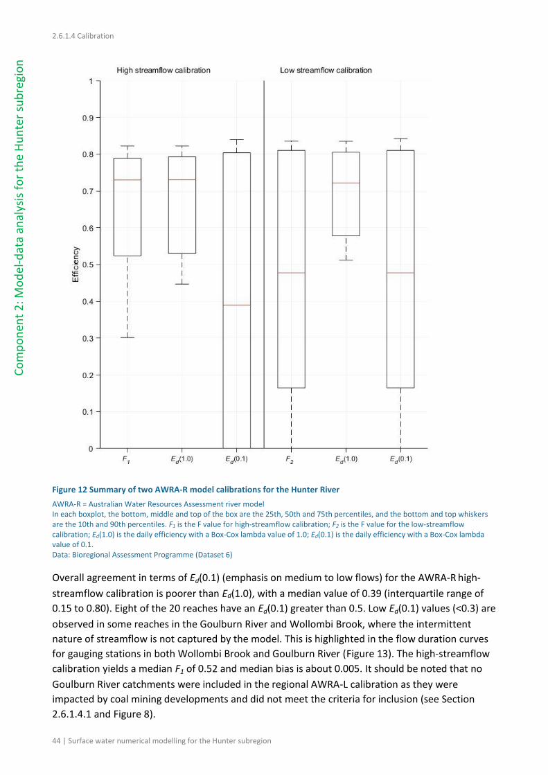
2.6.1.4 Calibration
44 | Surface water numerical modelling for the Hunter subregion
Co
mp
on
ent
2: M
od
el-d
ata
anal
ysis
fo
r th
e H
un
ter
sub
regi
on
Figure 12 Summary of two AWRA-R model calibrations for the Hunter River
AWRA-R = Australian Water Resources Assessment river model In each boxplot, the bottom, middle and top of the box are the 25th, 50th and 75th percentiles, and the bottom and top whiskers are the 10th and 90th percentiles. F1 is the F value for high-streamflow calibration; F2 is the F value for the low-streamflow calibration; Ed(1.0) is the daily efficiency with a Box-Cox lambda value of 1.0; Ed(0.1) is the daily efficiency with a Box-Cox lambda value of 0.1. Data: Bioregional Assessment Programme (Dataset 6)
Overall agreement in terms of Ed(0.1) (emphasis on medium to low flows) for the AWRA-R high-
streamflow calibration is poorer than Ed(1.0), with a median value of 0.39 (interquartile range of
0.15 to 0.80). Eight of the 20 reaches have an Ed(0.1) greater than 0.5. Low Ed(0.1) values (<0.3) are
observed in some reaches in the Goulburn River and Wollombi Brook, where the intermittent
nature of streamflow is not captured by the model. This is highlighted in the flow duration curves
for gauging stations in both Wollombi Brook and Goulburn River (Figure 13). The high-streamflow
calibration yields a median F1 of 0.52 and median bias is about 0.005. It should be noted that no
Goulburn River catchments were included in the regional AWRA-L calibration as they were
impacted by coal mining developments and did not meet the criteria for inclusion (see Section
2.6.1.4.1 and Figure 8).
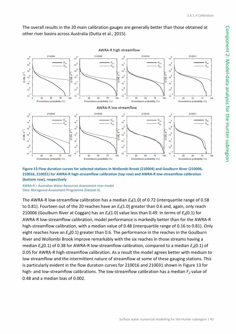
2.6.1.4 Calibration
Surface water numerical modelling for the Hunter subregion | 45
Co
mp
on
ent 2
: Mo
del-d
ata analysis fo
r the
Hu
nter su
bregio
n
The overall results in the 20 main calibration gauges are generally better than those obtained at
other river basins across Australia (Dutta et al., 2015).
Figure 13 Flow duration curves for selected stations in Wollombi Brook (210004) and Goulburn River (210006,
210016, 210031) for AWRA-R high-streamflow calibration (top row) and AWRA-R low-streamflow calibration
(bottom row), respectively
AWRA-R = Australian Water Resources Assessment river model Data: Bioregional Assessment Programme (Dataset 6)
The AWRA-R low-streamflow calibration has a median Ed(1.0) of 0.72 (interquartile range of 0.58
to 0.81). Fourteen out of the 20 reaches have an Ed(1.0) greater than 0.6 and, again, only reach
210006 (Goulburn River at Coggan) has an Ed(1.0) value less than 0.49. In terms of Ed(0.1) for
AWRA-R low-streamflow calibration, model performance is markedly better than for the AWRA-R
high-streamflow calibration, with a median value of 0.48 (interquartile range of 0.16 to 0.81). Only
eight reaches have an Ed(0.1) greater than 0.6. The performance in the reaches in the Goulburn
River and Wollombi Brook improve remarkably with the six reaches in those streams having a
median Ed(0.1) of 0.38 for AWRA-R low-streamflow calibration, compared to a median Ed(0.1) of
0.05 for AWRA-R high-streamflow calibration. As a result the model agrees better with medium to
low streamflow and the intermittent nature of streamflow at some of these gauging stations. This
is particularly evident in the flow duration curves for 210016 and 210031 shown in Figure 13 for
high- and low-streamflow calibrations. The low-streamflow calibration has a median F2 value of
0.48 and a median bias of 0.002.

2.6.1.4 Calibration
46 | Surface water numerical modelling for the Hunter subregion
Co
mp
on
ent
2: M
od
el-d
ata
anal
ysis
fo
r th
e H
un
ter
sub
regi
on
Table 7 Summary of AWRA-R calibration for the 20 reaches in the Hunter subregion
Streamflow gauge ID
Mean annual
streamflow (ML/y)
High-streamflow calibration Low-streamflow calibration
F1 Ed(1.0) Ed(0.1) F2 Ed(1.0) Ed(0.1)
210001 524 0.74 0.74 0.83 0.83 0.74 0.83
210002 248 0.73 0.73 0.80 0.80 0.72 0.80
210004 112 0.53 0.53 –0.22 0.20 0.63 0.20
210006 70 0.21 0.21 –0.28 0.07 0.25 0.07
210016 96 0.69 0.69 0.45 0.69 0.68 0.69
210028 76 0.79 0.79 –0.04 0.21 0.84 0.21
210031 152 0.73 0.73 –0.03 0.58 0.72 0.58
210044 55 0.53 0.53 0.42 0.16 0.56 0.16
210052 70 0.66 0.66 0.20 0.38 0.69 0.38
210055 241 0.79 0.79 0.77 0.78 0.79 0.78
210056 234 0.81 0.81 0.81 0.82 0.82 0.82
210064 624 0.89 0.89 0.81 0.82 0.89 0.82
210083 356 0.81 0.81 –4.16 –4.56 0.82 –4.56
210088 11 –1.11 0.55 –4.92 –5.55 0.53 –4.47
210089 24 0.52 0.52 0.35 –0.20 0.57 –0.20
210127 337 0.76 0.76 0.90 0.91 0.76 0.91
210128 362 0.78 0.79 0.85 0.84 0.79 0.85
210131 50 0.50 0.50 0.30 0.43 0.58 0.43
210134 440 0.83 0.83 0.52 0.52 0.83 0.52
210135 59 0.39 0.39 –0.18 0.17 0.49 0.17
Median 132 0.73 0.73 0.39 0.48 0.72 0.48
AWRA-R = Australian Water Resources Assessment river model; F1 = F value for high-streamflow calibration; F2 = F value for low-streamflow calibration (see Viney, 2016); Ed(1.0) = daily efficiency with a Box-Cox lambda value of 1.0; Ed(0.1) = daily efficiency with a Box-Cox lambda value of 0.1 Data: Bioregional Assessment Programme (Dataset 6)
The impact of including seven additional reaches on the calibration of AWRA-R generally degrades
agreement with observations in the reaches immediately downstream of these reaches. For
example, the median Ed(1.0) using the high-streamflow calibration with the additional reaches is
0.66 (range 0.12 to 0.88). The largest degradation is for the Hunter River at Denman (210055),
where Ed(1.0) decreases from 0.79 to 0.59, followed by Wollombi Brook at Bulga (210028) (0.77 to
0.63) and Hunter River at Liddell (210083) (0.81 to 0.67). Changes in Ed(1.0) are marginal (<0.05) in
the rest of the gauging stations. Again, median bias is less than 0.005.
Boxplots in Figure 14 show the bias of the two calibration schemes (AWRA-R high-streamflow and
AWRA-R low-streamflow calibration) in predicting the nine hydrological response variables that
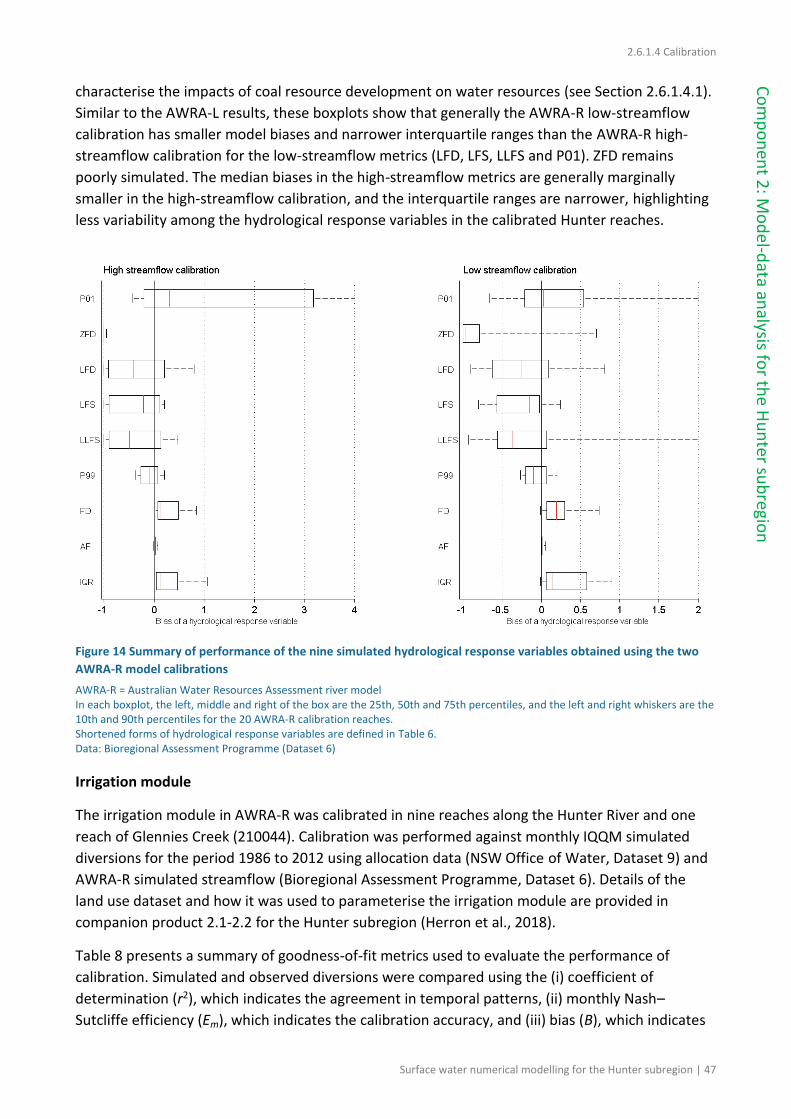
2.6.1.4 Calibration
Surface water numerical modelling for the Hunter subregion | 47
Co
mp
on
ent 2
: Mo
del-d
ata analysis fo
r the
Hu
nter su
bregio
n
characterise the impacts of coal resource development on water resources (see Section 2.6.1.4.1).
Similar to the AWRA-L results, these boxplots show that generally the AWRA-R low-streamflow
calibration has smaller model biases and narrower interquartile ranges than the AWRA-R high-
streamflow calibration for the low-streamflow metrics (LFD, LFS, LLFS and P01). ZFD remains
poorly simulated. The median biases in the high-streamflow metrics are generally marginally
smaller in the high-streamflow calibration, and the interquartile ranges are narrower, highlighting
less variability among the hydrological response variables in the calibrated Hunter reaches.
Figure 14 Summary of performance of the nine simulated hydrological response variables obtained using the two
AWRA-R model calibrations
AWRA-R = Australian Water Resources Assessment river model In each boxplot, the left, middle and right of the box are the 25th, 50th and 75th percentiles, and the left and right whiskers are the 10th and 90th percentiles for the 20 AWRA-R calibration reaches. Shortened forms of hydrological response variables are defined in Table 6. Data: Bioregional Assessment Programme (Dataset 6)
Irrigation module
The irrigation module in AWRA-R was calibrated in nine reaches along the Hunter River and one
reach of Glennies Creek (210044). Calibration was performed against monthly IQQM simulated
diversions for the period 1986 to 2012 using allocation data (NSW Office of Water, Dataset 9) and
AWRA-R simulated streamflow (Bioregional Assessment Programme, Dataset 6). Details of the
land use dataset and how it was used to parameterise the irrigation module are provided in
companion product 2.1-2.2 for the Hunter subregion (Herron et al., 2018).
Table 8 presents a summary of goodness-of-fit metrics used to evaluate the performance of
calibration. Simulated and observed diversions were compared using the (i) coefficient of
determination (r2), which indicates the agreement in temporal patterns, (ii) monthly Nash–
Sutcliffe efficiency (Em), which indicates the calibration accuracy, and (iii) bias (B), which indicates

2.6.1.4 Calibration
48 | Surface water numerical modelling for the Hunter subregion
Co
mp
on
ent
2: M
od
el-d
ata
anal
ysis
fo
r th
e H
un
ter
sub
regi
on
the overall tendency of the model towards overestimation or underestimation. Good diversion
patterns were simulated in all reaches, with a median r2 of 0.82 (range 0.71 to 0.91).
Table 8 Summary of AWRA-R irrigation calibration for nine reaches in the Hunter subregion
Streamflow gauge ID Mean annual irrigation diversion
(ML/y)
r2 Em B
210001 5215 0.88 0.77 0.00
210002 11789 0.88 0.74 –0.03
210044 853 0.76 0.52 –0.13
210055 5788 0.71 0.43 –0.03
210064 16142 0.91 0.79 0.03
210083 12516 0.86 0.71 –0.03
210127 760 0.82 0.67 –0.10
210128 356 0.76 0.56 0.03
210134 2020 0.71 0.49 0.03
Median 5215 0.82 0.67 -0.03
AWRA-R = Australian Water Resources Assessment river model; r2 = coefficient of determination; Em = monthly Nash–Sutcliffe efficiency; B = model bias Data: Bioregional Assessment Programme (Dataset 6), NSW Office of Water (Dataset 9)
Figure 15 shows time series of observed and simulated diversions for the four reaches of the
Hunter River with the highest water use. Inter-annual and intra-annual variability are generally
captured by the model, with a mean Em of 0.67 (range 0.43 to 0.79).
The variance in Em is greater than the variance in r2 (Table 8), indicating model overestimation or
underestimation (van Dijk et al., 2008). Diversions are under estimated in five reaches, but the
underestimation only exceeds 10% in reach 210044. The mean absolute bias in all reaches is 0.04.
Dam storage volumes, releases and allocations
Storage volumes for Glenbawn Dam and Glennies Creek Dam, releases and allocations were
calibrated as a whole system against observed daily storage volumes and IQQM simulated releases
(NSW Office of Water, Dataset 9). Individual dam volumes and releases were subsequently
estimated from the allocations and a split value based on IQQM simulated releases. The
calibration methodology and justification is described in companion submethodology M06 (as
listed in Table 1) for surface water modelling (Viney, 2016).
Goodness-of-fit metrics used to evaluate the performance on calibrated storage volumes and dam
releases included the monthly Nash–Sutcliffe efficiency (Em), the coefficient of determination (r2)
and the root-mean-square error (RMSE) to assess the overall accuracy.

2.6.1.4 Calibration
Surface water numerical modelling for the Hunter subregion | 49
Co
mp
on
ent 2
: Mo
del-d
ata analysis fo
r the
Hu
nter su
bregio
n
Figure 15 Example of IQQM and simulated monthly irrigation diversions for four reaches in the Hunter River
IQQM = Integrated Quantity-Quality Model Data: Bioregional Assessment Programme (Dataset 6), NSW Office of Water (Dataset 9)
For illustrative purposes, time series of monthly storage volumes are shown in Figure 16a and
Figure 16c. Temporal patterns agree well with observations, with r2 values of 0.87 and 0.89 for
Glenbawn Dam and Glennies Creek Dam, respectively. In contrast, modelled volumes are modest
for Glenbawn Dam (Em = 0.37) and poor for Glennies Creek Dam (Em = 0.1). The RMSE is 79 GL and
33 GL for Glenbawn Dam and Glennies Creek Dam, respectively, or about 15% of their mean
storage volumes. It can be seen in Figure 16 that AWRA-R generally under estimates storage
volumes between 1993 and 2002, but over estimates them during the dry period between 2003
and 2008.
Time series of monthly dam releases are shown in Figure 16b and Figure 16d. Temporal patterns
agree reasonably well with observations, with r2 values of 0.5 and 0.84 for Glenbawn Dam and
Glennies Creek Dam, respectively. Simulated releases are poor for Glenbawn Dam (Em = 0.01) but
good for Glennies Creek Dam (Em = 0.65). The RMSE for the calibration period (1993 to 2012) is
9.4 GL and 1.5 GL for Glenbawn Dam and Glennies Creek Dam releases, respectively.
Figure 17 summarises the monthly percentage error (computed as the percentage of the
difference between volume simulated and observed divided by simulated volume) for both dams.
The error is generally –20% to +20%, which suggests that the modelled allocations will generally
be within this margin of error.
0
1000
2000
3000
4000
5000
1986
1988
1990
1992
1994
1996
1998
2000
2002
2004
2006
2008
2010
2012
Div
ers
ion (
ML/m
o)
210002
IQQM Simulated
(a)
0
1000
2000
3000
4000
5000
1986
1988
1990
1992
1994
1996
1998
2000
2002
2004
2006
2008
2010
2012
Div
ers
ion (
ML/m
o)
210064
IQQM Simulated
(c)
0
1000
2000
3000
4000
5000
1986
1988
1990
1992
1994
1996
1998
2000
2002
2004
2006
2008
2010
2012
Div
ers
ion (
ML/m
o)
210055
IQQM Simulated
(b)
0
1000
2000
3000
4000
5000
1986
1988
1990
1992
1994
1996
1998
2000
2002
2004
2006
2008
2010
2012
Div
ers
ion (
ML/m
o)
210083
IQQM Simulated
(d)

2.6.1.4 Calibration
50 | Surface water numerical modelling for the Hunter subregion
Co
mp
on
ent
2: M
od
el-d
ata
anal
ysis
fo
r th
e H
un
ter
sub
regi
on
Figure 16 Observed and AWRA-R simulated monthly dam storage volume for (a) Glenbawn Dam and (c) Glennies
Creek Dam; and IQQM and AWRA-R simulated monthly releases for (b) Glenbawn Dam and (d) Glennies Creek Dam
AWRA-R = Australian Water Resources Assessment river model; IQQM = Integrated Quantity-Quality Model Data: Bioregional Assessment Programme (Dataset 6), NSW Office of Water (Dataset 9, Dataset 11)
The poor monthly efficiencies for the simulated releases from Glenbawn Dam can be attributed to
the imposed releases in December and January to satisfy water demand for the environment and
for electricity generation. Although electricity generation demand does not dominate the variance
in the dam releases (r2 = 0.15, whereas for irrigation and mine demand r2 = 0.27), it drives some of
the peak releases, particularly during the dry period of 2003–2008. As a result, the dam model
misses some of these peaks (i.e. those occurring in months other than December and January), or
simulates greater peaks in December and January. When only irrigation and mining demand are
considered, AWRA-R releases can explain 45% of the variance. In the case of Glennies Creek Dam
releases, the model conceptualisation captures well the downstream irrigation and mining
demand, which comprises about 100% of diversions.
Time series of observed and estimated allocations are shown in Figure 18. Simulated allocations
are less than 100% during 1995 to 1999 and during 2006 to 2008. Observed allocations are 100%
during 1995 to 1999 despite dam volumes being around 50% full; this may reflect changes in
licence volumes and/or policy that are not considered in the model. Allocations are over estimated
by the model in the second dry period (2006 to 2008) when dams are at around 30% of their
capacity, mainly because differences between simulated and observed dam volumes are about
30% and 50% for Glenbawn Dam and Glennies Creek Dam, respectively.
0
200
400
600
800
1993
1994
1995
1996
1997
1998
1999
2000
2001
2002
2003
2004
2005
2006
2007
2008
2009
2010
2011
2012
Volu
me (
GL)
Observed AWRA-R
(a)Glenbawn Dam
0
50
100
150
200
250
300
1993
1994
1995
1996
1997
1998
1999
2000
2001
2002
2003
2004
2005
2006
2007
2008
2009
2010
2011
2012
Volu
me (
GL)
Observed AWRA-R
(c)Glennies Creek Dam
0
10
20
30
40
50
1993
1994
1995
1996
1997
1998
1999
2000
2001
2002
2003
2004
2005
2006
2007
2008
2009
2010
2011
2012
Volu
me (
GL)
IQQM AWRA-R
(b)
0
5
10
15
1993
1994
1995
1996
1997
1998
1999
2000
2001
2002
2003
2004
2005
2006
2007
2008
2009
2010
2011
2012
Volu
me (
GL)
IQQM AWRA-R
(d)

2.6.1.4 Calibration
Surface water numerical modelling for the Hunter subregion | 51
Co
mp
on
ent 2
: Mo
del-d
ata analysis fo
r the
Hu
nter su
bregio
n
Figure 17 Percentage error for monthly dam storage volumes for Glenbawn Dam and for Glennies Creek Dam
Data: Bioregional Assessment Programme (Dataset 6), NSW Office of Water (Dataset 9)
Figure 18 Observed and AWRA-R simulated allocations for the AWRA-R Hunter river system
AWRA-R = Australian Water Resources Assessment river model Data: Bioregional Assessment Programme (Dataset 6), NSW Office of Water (Dataset 9)
Implications for model predictions
Overall, AWRA-R streamflow is reasonably well simulated using both high- and low-streamflow
calibrations. As expected, the low-streamflow calibration performed markedly better when the
evaluation was focused on the low flows, particularly in intermittent streams. The better
performance of the low-streamflow calibration was also observed in terms of the hydrological
response variables used to quantify the hydrological changes due to the additional coal resource
development, particularly for the variables characterising low streamflow, although the
performance for the variables characterising high flows was typically only marginally worse.
Generally, the hydrological response variables characterising low-streamflow conditions are under
0
25
50
75
100
1993 1994 1995 1996 1997 1998 1999 2000 2001 2002 2003 2004 2005 2006 2007 2008 2009 2010 2011 2012
Allo
cations (
%)
Observed AWRA-R

2.6.1.4 Calibration
52 | Surface water numerical modelling for the Hunter subregion
Co
mp
on
ent
2: M
od
el-d
ata
anal
ysis
fo
r th
e H
un
ter
sub
regi
on
estimated, whereas those characterising high-streamflow conditions are over estimated. The
number of ZFD remains poorly simulated with either model variant, though is slightly better for
the low-streamflow calibration.
Similar to AWRA-L calibrations, the parameter sets obtained for AWRA-R high- and low-
streamflow calibrations show large uncertainty in predicting the nine hydrological response
variables. Prior distributions of the model parameters are used in Approximate Bayesian
Computation uncertainty analysis to generate 3000 parameter sets which cover wide boundary
ranges for two of the AWRA-R calibration parameters (see Section 2.6.1.5). The outputs from
simulations that use the 3000 parameter sets for both AWRA-L and AWRA-R are expected to
provide suitable uncertainty bounds for predicting the hydrological changes due to the additional
coal resource development on the nine hydrological response variables in each model node in the
Hunter subregion (Section 2.6.1.6).
A wide range of dam operating conditions are represented in the model as a result of choosing a
20-year calibration period that included significant dry and wet periods. This ensures that the
model can be used in some of the extreme conditions imposed by modelling of the additional coal
resource development. The simple soil water deficit that computes releases for irrigation, and the
scheme (through a similar deficit proxy) that computes releases for mining perform reasonably
well. This is highlighted in the reasonably good agreement (r2 and Em both greater than 0.6)
between simulated and IQQM-modelled releases for Glennies Creek Dam, for which irrigation and
mining diversions comprise about 100% of surface water diversions; and by Glenbawn Dam
releases explaining 45% of the variance when only irrigation and mining demand are considered.
AWRA-R simulated dam storage volumes, releases and allocations are reasonable and comparable
to studies that simulated dam volumes and releases in multi-purpose reservoirs for scenario
modelling (see Wu and Chen, 2012). Most of the mismatch can be attributed to imposing a pattern
of summer dam releases for the environment and for electricity generation (the largest water user
in the Hunter river basin) on the model, which does not accurately reflect the actual demand
pattern. It is acknowledged that a more robust scheme is needed to simulate releases to satisfy
water demand for electricity generation.
Overestimation of releases during the dry period between 2003 and 2008 can be partly explained
by high water demand for electricity generation, but also by AWRA-L inflows to both dams, as
AWRA-L tends to over estimate streamflow in the Hunter River during this drought period.
Moreover, the calibration scheme uses one parameter per dam that linearly scales these inflows,
thus it is difficult to solve this issue through calibration of the AWRA-R dam module only.
Improvement of model performance can be achieved through better model conceptualisation and
calibration strategies.
References
Box GEP and Cox DR (1964) An analysis of transformations. Journal of the Royal Statistical Society
Series B, 26, 211–252.
Dutta D, Kim S, Hughes J, Vaze J and Yang A (2015) AWRA‐R v5.0 technical report. CSIRO Land and
Water, Australia.

2.6.1.4 Calibration
Surface water numerical modelling for the Hunter subregion | 53
Co
mp
on
ent 2
: Mo
del-d
ata analysis fo
r the
Hu
nter su
bregio
n
Herron NF, Frery E, Crosbie R, Pena-Arancibia J, Zhang YQ, Viney N, Rachakonda PK, Ramage A,
Marvanek SP, Gresham M, McVicar TR, Wilkins A (2018) Observations analysis, statistical
analysis and interpolation for the Hunter subregion. Product 2.1-2.2 for the Hunter
subregion from the Northern Sydney Basin Bioregional Assessment. Department of the
Environment and Energy, Bureau of Meteorology, CSIRO and Geoscience Australia, Australia.
http://data.bioregionalassessments.gov.au/product/NSB/HUN/2.1-2.2.
van Dijk AIJM, Kirby JM, Paydar Z, Podger G, Mainuddin M, Marvanek S and Peña-Arancibia J
(2008) Uncertainty in river modelling across the Murray-Darling Basin. A report to the
Australian Government from the CSIRO Murray-Darling Basin Sustainable Yields Project.
CSIRO, Canberra.
Viney N (2016) Surface water modelling. Submethodology M06 from the Bioregional Assessment
Technical Programme. Department of the Environment and Energy, Bureau of Meteorology,
CSIRO and Geoscience Australia, Australia.
http://data.bioregionalassessments.gov.au/submethodology/M06.
Viney NR, Vaze J, Wang B, Zhang Y, Yang A, Vleeshouwer J, Ramchurn A and Frost A (2014)
Intercomparison of methods for regionalising rainfall-runoff model predictions over large
domains. Proceedings of Hydrology and Water Resources Symposium, Perth, Australia, 970–
977.
Wu Y and Chen J (2012) An operation-based scheme for a multiyear and multipurpose reservoir to
enhance macroscale hydrologic models. Journal of Hydrometeorology 13, 270–283.
Datasets
Dataset 1 Bureau of Meteorology (2013) BILO Gridded Climate Data: Daily Climate Data for each
year from 1900 to 2012. Bioregional Assessment Source Dataset. Viewed 28 January 2016,
http://data.bioregionalassessments.gov.au/dataset/7aaf0621-a0e5-4b01-9333-
53ebcb1f1c14.
Dataset 2 Bioregional Assessment Programme (2015) Hunter SW data v2 20140724. Bioregional
Assessment Derived Dataset. Viewed 24 September 2015,
http://data.bioregionalassessments.gov.au/dataset/1934f57d-c6d6-43d1-abcd-
1cf957f3e7e2.
Dataset 3 Bioregional Assessment Programme (2014) Selected streamflow gauges within and near
the Hunter subregion. Bioregional Assessment Derived Dataset. Viewed 02 March 2016,
http://data.bioregionalassessments.gov.au/dataset/e83b0500-6254-47e1-b103-
5e6b5961fe6f.
Dataset 4 Bioregional Assessment Programme (2016) HUN AWRA-L Calibration Catchments v01.
Bioregional Assessment Derived Dataset. Viewed 21 July 2016,
http://data.bioregionalassessments.gov.au/dataset/c60e96db-f2a2-4036-9a2e-
353de289a715.
2.6.1.4 Calibration
54 | Surface water numerical modelling for the Hunter subregion
Co
mp
on
ent
2: M
od
el-d
ata
anal
ysis
fo
r th
e H
un
ter
sub
regi
on
Dataset 5 Bureau of Meteorology (2011) Geofabric Surface Cartography, v2.1. Bioregional
Assessment Source Dataset. Viewed 21 April 2015,
http://data.bioregionalassessments.gov.au/dataset/5342c4ba-f094-4ac5-a65d-
071ff5c642bc.
Dataset 6 Bioregional Assessment Programme (2016) HUN AWRA-LR Model v01. Bioregional
Assessment Derived Dataset. Viewed 07 December 2016,
http://data.bioregionalassessments.gov.au/dataset/670de516-30c5-4724-bd76-
8ff4a42ca7a5.
Dataset 7 Bioregional Assessment Programme (2016) HUN AWRA-R calibration catchments v01.
Bioregional Assessment Derived Dataset. Viewed 17 February 2016,
http://data.bioregionalassessments.gov.au/dataset/d419aae0-1cb3-48a8-82de-
941398a80e3a.
Dataset 8 Bioregional Assessment Programme (2016) HUN AWRA-R calibration nodes v01.
Bioregional Assessment Derived Dataset. Viewed 18 July 2016,
http://data.bioregionalassessments.gov.au/dataset/f2da394a-3d08-4cf4-8c24-
bf7751ea06a1.
Dataset 9 NSW Office of Water (2015) IQQM Model Simulation Regulated Rivers NSW DPI HUN
20150615. Bioregional Assessment Source Dataset. Viewed 07 December 2016,
http://data.bioregionalassessments.gov.au/dataset/d6e8c6f0-08bf-4ca6-bbef-
6ae0d79c34ce.
Dataset 10 Bioregional Assessment Programme (2016) HUN AWRA-R Simulation Node Cross
Sections v01. Bioregional Assessment Derived Dataset. Viewed 18 January 2016,
http://data.bioregionalassessments.gov.au/dataset/1fd9e5fe-eec1-4a34-8b4c-
6d95a54998df.
Dataset 11 NSW Office of Water (2016) HUN AWRA-R Observed storage volumes Glenbawn Dam
and Glennies Creek Dam. Bioregional Assessment Source Dataset. Viewed 08 September
2016, http://data.bioregionalassessments.gov.au/dataset/9c2dccdb-ef46-48c7-bfe1-
946ab57645e5.
2.6.1.5 Uncertainty
Surface water numerical modelling for the Hunter subregion | 55
Co
mp
on
ent 2
: Mo
del-d
ata analysis fo
r the
Hu
nter su
bregio
n
2.6.1.5 Uncertainty
Summary
The uncertainty analysis includes a qualitative assessment of the effect of model assumptions
on the predictions as well as a quantitative evaluation of the parameter uncertainty on the
predictions.
For each hydrological response variable, an ensemble of parameter combinations is selected
from a large range of parameter combinations that result in an acceptable match between
historically observed hydrological response variables and simulated equivalents.
This ensemble of parameter combinations is used to calculate the maximum raw change, the
maximum percent change and the year of maximum change for each hydrological variable at
each model node.
In the qualitative uncertainty analysis, the rationale behind the major assumptions and their
effect on predictions is discussed and scored. The assumption deemed to have the largest
effect on predictions is the implementation of the coal resource development pathway.
2.6.1.5.1 Quantitative uncertainty analysis
The aim of the quantitative uncertainty analysis is to provide probabilistic estimates of the
changes in the hydrological response variables due to coal resource development. A large number
of parameter combinations are evaluated and, in line with the Approximate Bayesian Computation
outlined in companion submethodology M09 (as listed in Table 1) for propagating uncertainty
through models (Peeters et al., 2016), only those parameter combinations that result in
acceptable model behaviour are accepted in the parameter ensemble used to make predictions.
Acceptable model behaviour is defined for each hydrological response variable based on the
capability of the model to reproduce historical, observed time series of the hydrological response
variable. For each hydrological response variable, a goodness of fit between model simulated and
observed annual hydrological response variable is defined and an acceptance threshold defined.
The ensemble of predictions are the changes in hydrological response variable simulated with the
parameter combinations for which the goodness of fit exceeds the acceptance threshold. The
resulting ensembles are presented and discussed in Section 2.6.1.6.
Parameter sampling
For AWRA-L, the parameters varied in the uncertainty analysis are those used in the calibration,
with the addition of the parameter for scaling effective porosity, ne_scale. For AWRA-R, two of
eight calibrated parameters, K_rout and Lag_rout, are included in the uncertainty analysis. The
remaining AWRA-R parameters are set to their values from the low-streamflow calibration and not
varied in the uncertainty analysis: variability in surface water – groundwater interactions (two
parameters) and catchment runoff (one parameter) is already captured in inputs from the
groundwater model and AWRA-L simulations; the three irrigation parameters are fixed as changes
in irrigation management are not in the scope of this study.
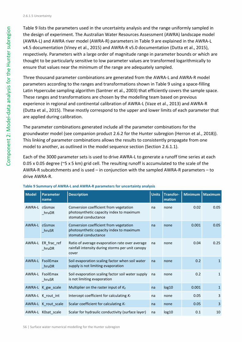
2.6.1.5 Uncertainty
56 | Surface water numerical modelling for the Hunter subregion
Co
mp
on
ent
2: M
od
el-d
ata
anal
ysis
fo
r th
e H
un
ter
sub
regi
on
Table 9 lists the parameters used in the uncertainty analysis and the range uniformly sampled in
the design of experiment. The Australian Water Resources Assessment (AWRA) landscape model
(AWRA-L) and AWRA river model (AWRA-R) parameters in Table 9 are explained in the AWRA-L
v4.5 documentation (Viney et al., 2015) and AWRA-R v5.0 documentation (Dutta et al., 2015),
respectively. Parameters with a large order of magnitude range in parameter bounds or which are
thought to be particularly sensitive to low parameter values are transformed logarithmically to
ensure that values near the minimum of the range are adequately sampled.
Three thousand parameter combinations are generated from the AWRA-L and AWRA-R model
parameters according to the ranges and transformations shown in Table 9 using a space-filling
Latin Hypercube sampling algorithm (Santner et al., 2003) that efficiently covers the sample space.
These ranges and transformations are chosen by the modelling team based on previous
experience in regional and continental calibration of AWRA-L (Vaze et al., 2013) and AWRA-R
(Dutta et al., 2015). These mostly correspond to the upper and lower limits of each parameter that
are applied during calibration.
The parameter combinations generated include all the parameter combinations for the
groundwater model (see companion product 2.6.2 for the Hunter subregion (Herron et al., 2018)).
This linking of parameter combinations allows the results to consistently propagate from one
model to another, as outlined in the model sequence section (Section 2.6.1.1).
Each of the 3000 parameter sets is used to drive AWRA-L to generate a runoff time series at each
0.05 x 0.05 degree (~5 x 5 km) grid cell. The resulting runoff is accumulated to the scale of the
AWRA-R subcatchments and is used – in conjunction with the sampled AWRA-R parameters – to
drive AWRA-R.
Table 9 Summary of AWRA-L and AWRA-R parameters for uncertainty analysis
Model Parameter name
Description Units Transfor-mation
Minimum Maximum
AWRA-L cGsmax
_hruDR
Conversion coefficient from vegetation photosynthetic capacity index to maximum stomatal conductance
na none 0.02 0.05
AWRA-L cGsmax
_hruSR
Conversion coefficient from vegetation photosynthetic capacity index to maximum stomatal conductance
na none 0.001 0.05
AWRA-L ER_frac_ref
_hruDR
Ratio of average evaporation rate over average rainfall intensity during storms per unit canopy cover
na none 0.04 0.25
AWRA-L FsoilEmax
_hruDR
Soil evaporation scaling factor when soil water supply is not limiting evaporation
na none 0.2 1
AWRA-L FsoilEmax
_hruSR
Soil evaporation scaling factor soil water supply is not limiting evaporation
na none 0.2 1
AWRA-L K_gw_scale Multiplier on the raster input of Kg na log10 0.001 1
AWRA-L K_rout_int Intercept coefficient for calculating Kr na none 0.05 3
AWRA-L K_rout_scale Scalar coefficient for calculating Kr na none 0.05 3
AWRA-L K0sat_scale Scalar for hydraulic conductivity (surface layer) na log10 0.1 10
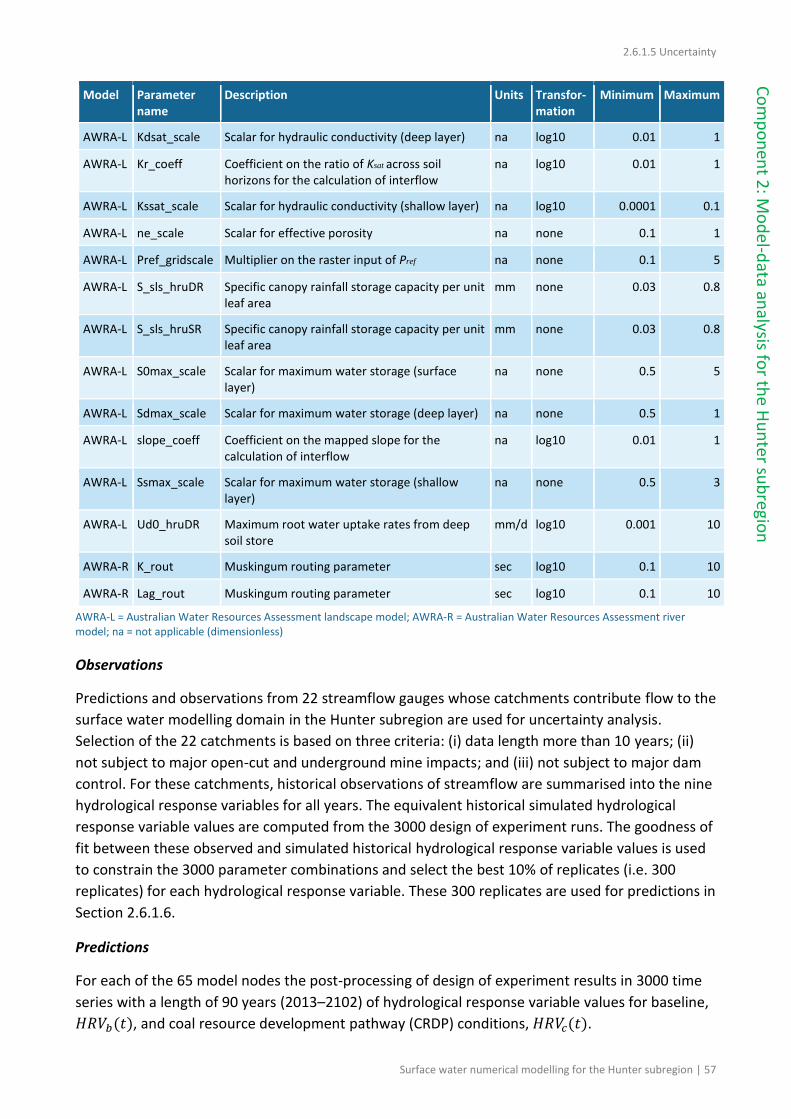
2.6.1.5 Uncertainty
Surface water numerical modelling for the Hunter subregion | 57
Co
mp
on
ent 2
: Mo
del-d
ata analysis fo
r the
Hu
nter su
bregio
n
Model Parameter name
Description Units Transfor-mation
Minimum Maximum
AWRA-L Kdsat_scale Scalar for hydraulic conductivity (deep layer) na log10 0.01 1
AWRA-L Kr_coeff Coefficient on the ratio of Ksat across soil horizons for the calculation of interflow
na log10 0.01 1
AWRA-L Kssat_scale Scalar for hydraulic conductivity (shallow layer) na log10 0.0001 0.1
AWRA-L ne_scale Scalar for effective porosity na none 0.1 1
AWRA-L Pref_gridscale Multiplier on the raster input of Pref na none 0.1 5
AWRA-L S_sls_hruDR Specific canopy rainfall storage capacity per unit leaf area
mm none 0.03 0.8
AWRA-L S_sls_hruSR Specific canopy rainfall storage capacity per unit leaf area
mm none 0.03 0.8
AWRA-L S0max_scale Scalar for maximum water storage (surface layer)
na none 0.5 5
AWRA-L Sdmax_scale Scalar for maximum water storage (deep layer) na none 0.5 1
AWRA-L slope_coeff Coefficient on the mapped slope for the calculation of interflow
na log10 0.01 1
AWRA-L Ssmax_scale Scalar for maximum water storage (shallow layer)
na none 0.5 3
AWRA-L Ud0_hruDR Maximum root water uptake rates from deep soil store
mm/d log10 0.001 10
AWRA-R K_rout Muskingum routing parameter sec log10 0.1 10
AWRA-R Lag_rout Muskingum routing parameter sec log10 0.1 10
AWRA-L = Australian Water Resources Assessment landscape model; AWRA-R = Australian Water Resources Assessment river model; na = not applicable (dimensionless)
Observations
Predictions and observations from 22 streamflow gauges whose catchments contribute flow to the
surface water modelling domain in the Hunter subregion are used for uncertainty analysis.
Selection of the 22 catchments is based on three criteria: (i) data length more than 10 years; (ii)
not subject to major open-cut and underground mine impacts; and (iii) not subject to major dam
control. For these catchments, historical observations of streamflow are summarised into the nine
hydrological response variables for all years. The equivalent historical simulated hydrological
response variable values are computed from the 3000 design of experiment runs. The goodness of
fit between these observed and simulated historical hydrological response variable values is used
to constrain the 3000 parameter combinations and select the best 10% of replicates (i.e. 300
replicates) for each hydrological response variable. These 300 replicates are used for predictions in
Section 2.6.1.6.
Predictions
For each of the 65 model nodes the post-processing of design of experiment results in 3000 time
series with a length of 90 years (2013–2102) of hydrological response variable values for baseline,
𝐻𝑅𝑉𝑏(𝑡), and coal resource development pathway (CRDP) conditions, 𝐻𝑅𝑉𝑐(𝑡).

2.6.1.5 Uncertainty
58 | Surface water numerical modelling for the Hunter subregion
Co
mp
on
ent
2: M
od
el-d
ata
anal
ysis
fo
r th
e H
un
ter
sub
regi
on
These two time series are summarised through the maximum raw change (amax), the maximum
percent change (pmax) and the year of maximum change (tmax). The percent change is defined
as:
𝑝𝑚𝑎𝑥 =𝑎𝑚𝑎𝑥
𝐻𝑅𝑉𝑏(𝑡𝑚𝑎𝑥)∗ 100 (1)
As the predictions include the effect of surface water – groundwater interaction through coupling
with the groundwater models, groundwater parameters will also affect the surface water
predictions.
Selection of parameter combinations
The acceptance threshold for each hydrological response variable is set to the 90th percentile of
the average goodness of fit between observed and simulated historical hydrological response
variable values obtained from nodes at 22 streamflow gauging sites. This means that out of the
3000 model replicates, the 300 best (or 10% best) are selected for each hydrological response
variable.
The selection of the 10% threshold is based on two considerations: (i) guaranteeing enough
prediction samples to ensure numerical robustness; and (ii) their performance approaching that
obtained from the high- and low-streamflow model calibrations. Furthermore, it is expected that
the full 3000 replicates contain many with infeasible parameter combinations (caused, for
example, by parameter correlations that are not considered in the independent random sampling)
and that these are likely to be filtered out by sampling only the best 10% of replicates.
Nevertheless, selecting the best 10% of replicates is determined arbitrarily, and the strength and
weakness of this decision are further discussed in Section 2.6.1.5.2.
2.6.1.5.2 Qualitative uncertainty analysis
The major assumptions and model choices underpinning the Hunter subregion surface water
model are listed in Table 10. The goal of the qualitative uncertainty analysis is to provide a non-
technical overview of the model assumptions, and their justification and effect on predictions, as
judged by the modelling team. This will also assist in an open and transparent review of the
modelling.
Each assumption in Table 10 is rated against three attributes (data, resources, technical) and their
effect on predictions.
1. The data column is the degree to which the question ‘If more or different data were
available, would this assumption/choice still have been made?’ would be answered
positively. A low rating indicates the assumption is not influenced by data availability, while
a high rating indicates that this choice would be revisited if more data were available.
2. The resources rating reflects the extent to which resources available for the modelling, such
as computing resources, personnel and time, influenced this assumption or model choice.
Again, a low rating indicates the same assumption would have been made with unlimited
resources, while a high rating indicates the assumption is driven by resource constraints.

2.6.1.5 Uncertainty
Surface water numerical modelling for the Hunter subregion | 59
Co
mp
on
ent 2
: Mo
del-d
ata analysis fo
r the
Hu
nter su
bregio
n
3. The technical rating reflects the extent to which the assumption is influenced by technical
and computational issues. A high rating flags assumptions and model choices that are
predominantly driven by computational or technical limitations of the model code. These
include issues related to spatial and temporal resolution of the models.
The most important rating relates to the effect the assumption or model choice has on the
predictions. This is a qualitative assessment by the modelling team of the extent to which a model
choice will affect the model predictions, with low indicating a minimal effect and high a large
effect.
Table 10 Qualitative uncertainty analysis as used for the Hunter subregion surface water model
Assumption or model choice Data Resources Technical Effect on predictions
Selection of calibration catchments Medium Low Low Low
High-flow and low-flow objective function Low Low High Low
Selection of goodness-of-fit function for each hydrological response variable
Low Low Low Low
Selection of acceptance threshold for uncertainty analysis Medium High Medium Medium
Interaction with the groundwater model Medium Medium High Medium
Implementation of the coal resource development pathway
High Low Low High
Streamflow routing Low Low Low Low
A discussion of each of the assumptions, including the rationale for the scoring, follows.
Selection of calibration catchments
The parameters that control the transformation of rainfall into streamflow are adjusted based on
a comparison of observed and simulated historical streamflow. Only a limited number of the
model nodes have historical streamflow. To calibrate the surface water model, a number of
catchments are selected outside the Hunter subregion. The parameter combinations that achieve
an acceptable agreement with observed flows are deemed acceptable for all catchments in the
subregion.
The selection of calibration catchments is therefore almost solely based on data availability, which
results in a medium score for this criterion. As it is technically trivial to include more calibration
catchments in the calibration procedure and as it would not appreciably change the computing
time required, both the resources and technical columns have a low rating.
The regionalisation methodology is valid as long as the selected catchments for calibration are not
substantially incompatible with those in the prediction domain in terms of size, climate, land use,
topography, geology and geomorphology. The majority of these assumptions can be considered
valid (see Section 2.6.1.6) and the overall effect on the predictions is therefore deemed to be low.

2.6.1.5 Uncertainty
60 | Surface water numerical modelling for the Hunter subregion
Co
mp
on
ent
2: M
od
el-d
ata
anal
ysis
fo
r th
e H
un
ter
sub
regi
on
High-flow and low-flow objective function
AWRA-L simulates daily streamflow. High-streamflow and low-streamflow conditions are governed
by different aspects of the hydrological system and it is difficult for any streamflow model to find
parameter sets that are able to adequately simulate both extremes of the hydrograph. In
recognition of this issue, two objective functions are chosen, one tailored to medium and high
flows and another one tailored to low flows.
Even with more calibration catchments and more time available for calibration, a high-flow and
low-flow objective function would still be necessary to find parameter sets suited to simulate
different aspects of the hydrograph. Data and resources are therefore scored low, while the
technical criterion is scored high.
The high-streamflow objective function is a weighted sum of the Nash–Sutcliffe efficiency (E) and
the bias. The former is most sensitive to differences in simulated and observed daily and monthly
streamflow, while the latter is most affected by the discrepancy between long-term observed and
simulated streamflow. The weighting of both components represents the trade-off between
simulating short-term and long-term streamflow behaviour. It also reflects the fact that some
parameters are more sensitive to daily behaviour and some are more sensitive to long-term
hydrology.
The low-streamflow objective function is achieved by transforming the observed and simulated
streamflow through a Box-Cox transformation (see Section 2.6.1.4). By this transformation, a small
number of large discrepancies in high streamflow will have less prominence in the objective
function than a large number of small discrepancies in low streamflow. Like the high-streamflow
objective function, the low-streamflow objective function consists of two components, the E
transformed by a Box-Cox power of 0.1 and bias, which again represent the trade-off between
short-term and long-term accuracy.
The choice of the weights between both terms in both objective functions is based on the
experience of the modelling team (Viney et al., 2009). The choice is not constrained by data,
technical issues or available resources. While different choices of the weights will result in a
different set of optimised parameter values, experience in the Water Information Research and
Development Alliance (WIRADA) project, in which the AWRA-L is calibrated on a continental scale,
has shown the calibration to be fairly robust against the weights in the objective function (Vaze
et al., 2013).
While the selection of objective function and its weights is a crucial step in the surface water
modelling process, the overall effect on the predictions is marginal through the uncertainty
analysis, hence the low rating.
Selection of goodness-of-fit function for each hydrological response variable
The goodness-of-fit function for each hydrological response variable for uncertainty analysis
has a very similar role to the objective function in calibration. Where the calibration focuses
on identifying a single parameter set that provides an overall good fit between observed and
simulated values, the uncertainty analysis aims to select an ensemble of parameter combinations
that are best suited to make the chosen prediction.

2.6.1.5 Uncertainty
Surface water numerical modelling for the Hunter subregion | 61
Co
mp
on
ent 2
: Mo
del-d
ata analysis fo
r the
Hu
nter su
bregio
n
Within the context of the bioregional assessment (BA), the calibration aims to provide a parameter
set that performs well at a daily resolution, while the uncertainty analysis focuses on specific
aspects of the yearly hydrograph.
The goodness-of-fit function is tailored to each hydrological response variable and averaged over
a number of selected catchments that contribute to flow in the Hunter subregion modelling
domain. This ensures parameter combinations are chosen that are able to simulate the specific
part of the hydrograph relevant to the hydrological response variable, at a local scale.
Like the objective function selection, the choice of summary statistic is primarily guided by the
predictions and to a much lesser extent by the available data, technical issues or resources. This is
the reason for the low rating for these attributes.
The impact on the predictions is deemed low as it is an unbiased estimate of model mismatch and
because it summarises the same aspect of the hydrograph as is needed for the prediction.
Selection of acceptance threshold for uncertainty analysis
The acceptance threshold ideally is independently defined based on an analysis of the system (see
companion submethodology M09 (as listed in Table 1) for propagating uncertainty through
models (Peeters et al., 2016)). For the surface water hydrological response variables, such an
independent threshold definition can be based on the observation uncertainty, which depends on
an analysis of the rating curves for each observation gauging station as well as at the model nodes.
There are limited rating curve data available, hence the medium rating. Even if this information
were available, the operational constraints within the BA prevent such a detailed analysis –
although it is technically feasible. The resources column therefore receives a high rating while the
technical column receives a medium rating.
The choice of setting the acceptance threshold equal to the 90th percentile of the summary
statistic for a particular hydrological response variable (i.e. selecting the best 10% of replicates) is
a subjective decision made by the modelling team. By varying this threshold through a trial-and-
error procedure in the testing phase of the uncertainty analysis methodology, the Assessment
team learned that this threshold is an acceptable trade-off between guaranteeing enough
prediction samples and overall good model performance. While relaxing the threshold may lead to
larger uncertainty intervals for the predictions, the median predicted values are considered robust
to this change. A formal test of this hypothesis has not yet been carried out. The effect on
predictions is therefore scored medium.
Interaction with the groundwater model
The coupling between the outputs of the groundwater model and the surface water models,
described in the model sequence section (Section 2.6.1.1), represents a pragmatic solution to
account for surface water – groundwater interactions at a regional scale. Even if a suitable
algorithm for integrated coupling of fluxes between the surface water and groundwater models
were available, the differences in spatial and temporal resolution would require non-trivial
upscaling and downscaling of spatio-temporal distributions of fluxes. For these reasons and also
for practical reasons related to run times and computational storage issues, the modelling
methodology for the Hunter subregion involves a one-directional feed of changes in the

2.6.1.5 Uncertainty
62 | Surface water numerical modelling for the Hunter subregion
Co
mp
on
ent
2: M
od
el-d
ata
anal
ysis
fo
r th
e H
un
ter
sub
regi
on
groundwater flux to streams from the groundwater model, rather than a fully coupled
implementation. Thus the rating for the technical attribute is high.
The data and resources columns are rated medium because even if it were technically feasible to
fully integrate the models, the implementation would be constrained by the available data and
the operational constraints. In an integrated model, a simulation would likely involve multiple
iterations between the groundwater and stream components and increase the computational
load significantly.
The overall effect on predictions is rated as medium. While changes in baseflow are generally
small compared to runoff, the low flow regime can be sensitive to them.
Implementation of the coal resource development pathway
The CRDP is implemented through the interaction with the groundwater models and by removing
the fraction of runoff in the catchment that is intercepted by the mine footprint from the total
catchment runoff. The key choices that are made in implementing the CRDP are (i) determining
which mining developments are included, and (ii) deciding on the spatial and temporal
development of their hydrological footprints.
In catchments in which the mine footprint is only a small fraction of the total area of the
catchment, the precise delineation of the spatial extent of the mine footprint is not crucial to the
predictions. In catchments in which the footprint is a sizeable fraction, accurate delineation of the
mine footprint becomes very important.
Similarly, the temporal evolution of mine footprints is crucial as it will determine how long the
catchment will be affected. This is especially relevant for the post-mining rehabilitation of mine
sites, when it becomes possible again for runoff generated within the mine footprint to reach the
streams.
In the Hunter subregion, the accuracy of the mine footprints represented in the model largely
reflects the accuracy of the mine footprints published or provided by the mine proponents. This
therefore is one of the crucial aspects of the surface water model as it potentially has a high
impact on predictions and it is driven by data availability rather than availability of resources or
technical issues. The data attribute is therefore scored high, while the resources and technical
columns are scored low. The effect on predictions is scored high.
Streamflow routing
Streamflow routing is taken into account in the Hunter AWRA-R as the Hunter River is a large
system and routing can lag flows by several days. Streamflow routing is not taken into account in
the Macquarie-Tuggerah lakes basin since it is unregulated and sufficiently small that lags in
streamflow due to routing will be within a daily time step. The effect on the prediction of not
incorporating routing is therefore minimal. Given the small potential for impact, resourcing the
development of a river-routing model for this region was not warranted. All attributes are rated
low as it is technically feasible and within the operational constraints of the BA to carry out
streamflow routing. Doing so would only minimally affect the predictions.
2.6.1.5 Uncertainty
Surface water numerical modelling for the Hunter subregion | 63
Co
mp
on
ent 2
: Mo
del-d
ata analysis fo
r the
Hu
nter su
bregio
n
References
Dutta D, Kim S, Hughes J, Vaze J and Yang A (2015) AWRA‐R v5.0 technical report. CSIRO Land and
Water, Australia.
Herron NF, Peeters L, Crosbie R, Marvanek SP, Pagendam D, Ramage A, Rachakonda PK and
Wilkins A (2018) Groundwater numerical modelling for the Hunter subregion. Product 2.6.2
for the Hunter subregion from the Northern Sydney Basin Bioregional
Assessment. Department of the Environment and Energy, Bureau of Meteorology, CSIRO and
Geoscience Australia, Australia.
http://data.bioregionalassessments.gov.au/product/NSB/HUN/2.6.2.
Peeters L, Pagendam D, Gao L, Hosack G, Jiang W and Henderson B (2016) Propagating uncertainty
through models. Submethodology M09 from the Bioregional Assessment Technical
Programme. Department of the Environment and Energy, Bureau of Meteorology, CSIRO and
Geoscience Australia, Australia.
http://data.bioregionalassessments.gov.au/submethodology/M09.
Santner TJ, Williams BJ and Notz WI (2003) The design and analysis of computer experiments.
Springer, New York.
Vaze J, Viney NR, Stenson MP, Renzullo LJ, Van Dijk AIJM, Dutta D, Crosbie R, Lerat J, Penton D,
Vleeshouwer J, Peeters LJM, Teng J, Kim S, Hughes J, Dawes W, Zhang Y, Leighton B, Perraud
JM, Joehnk JYA, Wang B, Frost A, Elmahdi A, Smith A and Daamen C (2013) The Australian
Water Resource Assessment modelling system (AWRA). MODSIM2013, 20th International
Congress on Modelling and Simulation. Modelling and Simulation Society of Australia and
New Zealand, December 2013, 3015–3021.
Viney N, Perraud J, Vaze J, Chiew F, Post D and Yang A (2009) The usefulness of bias constraints in
model calibration for regionalisation to ungauged catchments. 18th World IMACS Congress
and MODSIM09 International Congress on Modelling and Simulation, 13–17.
Viney N, Vaze J, Crosbie R, Wang B, Dawes W and Frost A (2015) AWRA-L v4.5: technical
description of model algorithms and inputs. CSIRO, Australia.

2.6.1.5 Uncertainty
64 | Surface water numerical modelling for the Hunter subregion
Co
mp
on
ent
2: M
od
el-d
ata
anal
ysis
fo
r th
e H
un
ter
sub
regi
on

2.6.1.6 Prediction
Surface water numerical modelling for the Hunter subregion | 65
Co
mp
on
ent 2
: Mo
del-d
ata analysis fo
r the
Hu
nter su
bregio
n
2.6.1.6 Prediction
Summary
Section 2.6.1.6 summarises prediction results of hydrological changes for nine hydrological
response variables due to the modelled additional coal resource development. The
hydrological changes on each model node were generated from among 3000 replicates
of the model runs using randomly selected parameter sets.
The prediction results show that the additional coal resource development in the Hunter
subregion can cause substantial changes in the hydrological response variables. The
comparison among the 65 model nodes shows that for the hydrological response variables
that characterise high-streamflow conditions, the relative hydrological changes are
particularly evident at model nodes where the footprint forms a large proportion of the
node catchment.
In general, the hydrological changes are greater in the small tributaries of the Hunter River
than in the model nodes along the river itself. The biggest hydrological changes (flow
reductions of up to 80%) occur at nodes 7 to 9 (Loders Creek, including Doctors Creek),
which enter the Hunter River just upstream of Singleton, and at nodes 52 (Dry Creek) and
55 (unnamed creek) in the vicinity of Muswellbrook. The catchments of nodes 7 to 9 include
the Bulga and Mount Thorley–Warkworth mines, while the catchments of nodes 52 and 55
include the Bengalla and Mount Pleasant mines. The prediction that the biggest hydrological
changes occur downstream of multiple mine developments highlights the cumulative nature
of potential hydrological changes, particularly on low-flow characteristics.
The hydrological changes due to the additional coal resource development on the low-
streamflow hydrological response variables appear to be slightly larger than those on the
high-streamflow hydrological response variables. However, the uncertainties in the predicted
change and the timing of the maximum change are greater for the low-streamflow
hydrological response variables.
The results suggest that changes to low-flow characteristics are caused by a combination
of the instantaneous effect of interception from the additional mine footprints and the
cumulative effect on baseflow over time caused by watertable drawdown, while the changes
to high-flow characteristics are dominated by direct interception of runoff.
2.6.1.6.1 Introduction
Section 2.6.1.6 summarises the prediction results for nine hydrological response variables and
for 65 surface water model nodes. The nine hydrological response variables for streamflow are:
AF – the annual flow volume (GL/year)
P99 – the daily streamflow rate at the 99th percentile (ML/day)
IQR – the interquartile range in daily streamflow (ML/day); that is, the difference between
the daily streamflow rate at the 75th percentile and at the 25th percentile
2.6.1.6 Prediction
66 | Surface water numerical modelling for the Hunter subregion
Co
mp
on
ent
2: M
od
el-d
ata
anal
ysis
fo
r th
e H
un
ter
sub
regi
on
FD – the number of high-flow days per year. The threshold for high-flow days is the 90th
percentile from the simulated 90-year period (2013 to 2102). In some early products, this
was referred to as ‘flood days’
P01 – the daily streamflow rate at the 1st percentile (ML/day)
ZFD – the number of zero-flow days each year
LFD – the number of low-flow days per year. The threshold for low-flow days is the 10th
percentile from the simulated 90-year period (2013 to 2102)
LFS – the number of low-flow spells per year. A spell is defined as a period of contiguous
days of streamflow below the 10th percentile threshold
LLFS – the length (days) of the longest low-flow spell each year.
These hydrological response variables were chosen to be able to quantify changes across the
entire flow regime (see submethodology M06 surface water modelling (Viney, 2016)). For each of
these hydrological response variables a time series of annual values for the period 2013 to 2102 is
constructed for each model node.
For each model node, 3000 sets of randomly selected parameter values were used to generate
3000 replicates of development impact. From these, the best 300 replicates for each hydrological
response variable – as assessed by their ability to predict that hydrological response variable at
the 22 observation sites – were chosen for further analysis. The 22 assessment nodes are chosen
for their availability of suitable observational data. Each boxplot was generated from the resulting
300 samples. The boxplots show the distributions over the 300 replicates of the maximum raw
change (amax) in each metric between the baseline and coal resource development pathway
(CRDP) predictions, the corresponding maximum percent change (pmax) and the year of maximum
change (tmax). In general, the most meaningful diagnostic for the flux-based metrics (P01, P99,
AF and IQR) will be pmax, while the most meaningful diagnostic for the frequency-based metrics
(LFD, LFS, LLFS, ZFD and FD) will be amax.
It is important to recognise that the amax and pmax values give the largest annual departure
between the baseline and CRDP predictions for the respective hydrological response variables.
As such, amax and pmax represent extreme responses. They do not represent the magnitudes
of responses that would be expected to occur every year.
Results are for those additional coal resource developments that were able to be modelled. As
discussed in companion product 2.3 (conceptual modelling) for the Hunter subregion (Dawes
et al., 2018), there was insufficient data to model West Muswellbrook and Mandalong
developments; Wambo and Mount Arthur developments were assessed as not causing any
additional impact on catchment runoff and therefore were not modelled; and the Chain Valley
extension is under Lake Macquarie and does not affect surface runoff. The potential effects
on surface water from developments at West Muswellbrook and Mandalong are considered
qualitatively in companion product 3-4 (impact and risk analysis) for the Hunter subregion
(as listed in Table 2).

2.6.1.6 Prediction
Surface water numerical modelling for the Hunter subregion | 67
Co
mp
on
ent 2
: Mo
del-d
ata analysis fo
r the
Hu
nter su
bregio
n
2.6.1.6.2 Results analysis
The predictions of hydrological change associated with additional coal resource development are
shown in the boxplots in Figure 19 to Figure 27. In these figures, the model nodes are grouped for
different river sections and tributaries. Within these groupings, small tributaries have a darker
background shading. Nodes are ordered from downstream to upstream. The tributary grouping
labelled ‘u/s Greta’ (u/s = upstream of) includes tributaries that join the Hunter River between
nodes 1 and 20. The tributary grouping labelled ‘u/s Glennies Creek’ includes tributaries that join
the Hunter River between nodes 25 and 51. The tributary grouping labelled ‘u/s Denman’ includes
tributaries that join the Hunter River above node 51. Refer to Figure 5 in Section 2.6.1.3 for a
schematic depiction of the model nodes and the network topology. The implications of these
hydrological changes on landscape classes and assets are not discussed here, but are the focus of
the impact and risk analysis reported in companion product 3-4 for the Hunter subregion (as listed
in Table 2).
Figure 19 shows the changes to the annual flow (AF) at the 65 model nodes. The biggest
percentage reductions occur in some of the small tributaries of the Hunter River, and range up to
a median pmax of 81% at node 8 (Doctors Creek). Nine model nodes have reductions in median
pmax that exceed 20%. Seven of these have catchment areas of less than 25 km2 and all have
areas of less than 80 km2. There are tightly constrained distributions of pmax values around
these median values at all the heavily affected nodes except for node 11, where the 5th to 95th
percentile range in pmax is –51% to –30%. Apart from reductions in median pmax of about 8% at
nodes 46 (Wollar Creek) and 47 (Wilpinjong Creek) there is little effect on AF in the nodes in the
Goulburn and Wyong river basins or in those along Wollombi Brook, where the median pmax
reductions are less than 2% of baseline flow. The largest reductions in median amax are located
in the lower Hunter River and increase with distance downstream. The biggest effects are at nodes
1 and 6 and result in losses of around 29 GL/year, which represent about 3% of the baseline flow.
A large proportion of this median reduction (13 GL/year) originates in the Loders Creek tributary
(node 7), with the remainder propagating from upstream (node 10).
For the heavily affected nodes, the median year at which maximum hydrological changes occurs is
either 2022 or 2037 for the tributaries of the lower Hunter River (nodes 7, 8, 9 and 11), but 2028
for tributaries upstream of Glennies Creek. There is relatively little uncertainty in these dates. The
maximum hydrological changes in the Hunter River itself tend to occur in 2037.

2.6.1.6 Prediction
68 | Surface water numerical modelling for the Hunter subregion
Co
mp
on
ent
2: M
od
el-d
ata
anal
ysis
fo
r th
e H
un
ter
sub
regi
on
Figure 19 Hydrological changes due to additional coal resource development on annual flow (AF) at the 65 model nodes within the Hunter subregion
amax = maximum raw change; pmax = maximum percent change; tmax = year of maximum change; u/s = upstream of; NI = negligible impact Numbers above the top panel are the median of the best 300 replicates under the baseline for the year corresponding to the median tmax. In each boxplot, the bottom, middle and top of the box are the 25th, 50th and 75th percentiles, and the bottom and top whiskers are the 5th and 95th percentiles. Within the groupings, small tributaries have a darker background shading. Refer to Figure 4 in Section 2.6.1.3 for location of model nodes. Data: Bioregional Assessment Programme (Dataset 1)
This figure has been optimised for printing on A3 paper (420 mm x 297 mm).
2.6.1.6 Prediction
Surface water numerical modelling for the Hunter subregion | 69
Co
mp
on
ent 2
: Mo
del-d
ata analysis fo
r the
Hu
nter su
bregio
n
Figure 20 shows the changes to the daily streamflow rate at the 99th percentile (P99) at each
model node. The biggest changes in pmax occur at the same nine locations with the biggest effect
on AF. For P99 the median pmax values for these nine nodes exceed 20% and range up to 68% for
node 52 (Dry Creek). At most of these sites there is a greater spread of pmax values than there is
for AF. At most of the affected nodes, the percentage reduction in P99 is greater than the
percentage reduction in AF.
The year of maximum change in P99 tends to correspond with the year of maximum change in AF,
with the exception that it occurs later in the heavily affected nodes 7 and 8 (2052 and 2049,
respectively).

2.6.1.6 Prediction
70 | Surface water numerical modelling for the Hunter subregion
Co
mp
on
ent
2: M
od
el-d
ata
anal
ysis
fo
r th
e H
un
ter
sub
regi
on
Figure 20 Hydrological changes due to additional coal resource development on daily streamflow at the 99th percentile (P99) at the 65 model nodes within the Hunter subregion
amax = maximum raw change; pmax = maximum percent change; tmax = year of maximum change; u/s = upstream of; NI = negligible impact Numbers above the top panel are the median of the best 300 replicates under the baseline for the year corresponding to the median tmax. In each boxplot, the bottom, middle and top of the box are the 25th, 50th and 75th percentiles, and the bottom and top whiskers are the 5th and 95th percentiles. Within the groupings, small tributaries have a darker background shading. Refer to Figure 4 in Section 2.6.1.3 for location of model nodes. Data: Bioregional Assessment Programme (Dataset 1)
This figure has been optimised for printing on A3 paper (420 mm x 297 mm).

2.6.1.6 Prediction
Surface water numerical modelling for the Hunter subregion | 71
Co
mp
on
ent 2
: Mo
del-d
ata analysis fo
r the
Hu
nter su
bregio
n
Figure 21 shows the changes to the interquartile range (IQR) at each model node. The changes in
IQR associated with the additional coal resource development are always reductions. This implies
that the difference in flow rates between high flows (the 75th percentile of daily streamflow) and
low flows (the 25th percentile of daily streamflow) is reduced, most likely through a decrease
in the 75th percentile. The patterns of change are similar to those of AF (Figure 19) and P99
(Figure 20). The biggest reductions in median pmax occur at nodes on small tributaries of the
Hunter River, and include reductions of more than 70% at nodes 8 (Doctors Creek), 52 (Dry Creek)
and 55 (unnamed creek west of Muswellbrook). Each of these nodes have catchment areas of less
than 25 km2.

2.6.1.6 Prediction
72 | Surface water numerical modelling for the Hunter subregion
Co
mp
on
ent
2: M
od
el-d
ata
anal
ysis
fo
r th
e H
un
ter
sub
regi
on
Figure 21 Hydrological changes due to additional coal resource development on interquartile range (IQR) at the 65 model nodes within the Hunter subregion
amax = maximum raw change; pmax = maximum percent change; tmax = year of maximum change; u/s = upstream of; NI = negligible impact Numbers above the top panel are the median of the best 300 replicates under the baseline for the year corresponding to the median tmax. In each boxplot, the bottom, middle and top of the box are the 25th, 50th and 75th percentiles, and the bottom and top whiskers are the 5th and 95th percentiles. Within the groupings, small tributaries have a darker background shading. Refer to Figure 4 in Section 2.6.1.3 for location of model nodes. Data: Bioregional Assessment Programme (Dataset 1)
This figure has been optimised for printing on A3 paper (420 mm x 297 mm).

2.6.1.6 Prediction
Surface water numerical modelling for the Hunter subregion | 73
Co
mp
on
ent 2
: Mo
del-d
ata analysis fo
r the
Hu
nter su
bregio
n
Figure 22 shows the changes to high-flow days (FD) at each model node. Once again, the largest
reductions in the number of FD occur in the small tributaries of the Hunter River, but there are
also largish reductions at two tributary nodes in the Goulburn river basin. The biggest change is a
maximum reduction in the median number of FD by 46 days/year at node 52 (Dry Creek). Twelve
nodes have median reductions in amax of more than 5 days/year. However, there is much greater
uncertainty around changes in the number of high-flow days (and in the timing of the maximum
changes) than there is for changes in AF. Along the Hunter River, the frequency of FD is reduced
by 4 days/year at node 6 (Singleton) and by lesser amounts elsewhere.

2.6.1.6 Prediction
74 | Surface water numerical modelling for the Hunter subregion
Co
mp
on
ent
2: M
od
el-d
ata
anal
ysis
fo
r th
e H
un
ter
sub
regi
on
Figure 22 Hydrological changes due to additional coal resource development on high-flow days (FD) at the 65 model nodes within the Hunter subregion
amax = maximum raw change; pmax = maximum percent change; tmax = year of maximum change; u/s = upstream of; NI = negligible impact Numbers above the top panel are the median of the best 300 replicates under the baseline for the year corresponding to the median tmax. In each boxplot, the bottom, middle and top of the box are the 25th, 50th and 75th percentiles, and the bottom and top whiskers are the 5th and 95th percentiles. Within the groupings, small tributaries have a darker background shading. Refer to Figure 4 in Section 2.6.1.3 for location of model nodes. Data: Bioregional Assessment Programme (Dataset 1)
This figure has been optimised for printing on A3 paper (420 mm x 297 mm).

2.6.1.6 Prediction
Surface water numerical modelling for the Hunter subregion | 75
Co
mp
on
ent 2
: Mo
del-d
ata analysis fo
r the
Hu
nter su
bregio
n
Figure 23 shows the changes to the daily streamflow rate at the 1st percentile (P01) at each model
node. Reductions in median pmax of more than 10% are predicted in many of the tributary nodes
with large reductions in high-flow characteristics, especially nodes 7, 8, 9, 11 and 55, including
100% reductions in median pmax at node 8 (Doctors Creek) and node 55 (unnamed). These cases
are representative of a particular year in a replicate for which there is a nonzero 1st percentile of
baseline flow, but the 1st percentile of CRDP flow is zero. Of particular note is that, despite
showing little change to the high-flow characteristics, there are substantial predicted changes to
1st percentile flow in the two nodes in the Wyong river basin, where the pmax values show
decreases of 51% (node 64) and 57% (node 65).
The timing of the maximum changes tends to be later for P01 than for the high-streamflow
hydrological response variables. The median tmax for P01 occurs in or later than 2044 at all of the
seven most heavily affected nodes.
By comparison to the three flux-based high-streamflow hydrological response variables (AF, IQR
and P99), P01 tends to have greater uncertainty – as shown by a large interquartile range relative
to the median response – for both pmax and tmax.

2.6.1.6 Prediction
76 | Surface water numerical modelling for the Hunter subregion
Co
mp
on
ent
2: M
od
el-d
ata
anal
ysis
fo
r th
e H
un
ter
sub
regi
on
Figure 23 Hydrological changes due to additional coal resource development on daily streamflow at the 1st percentile (P01) at the 65 model nodes within the Hunter subregion
amax = maximum raw change; pmax = maximum percent change; tmax = year of maximum change; u/s = upstream of; NI = negligible impact Numbers above the top panel are the median of the best 300 replicates under the baseline for the year corresponding to the median tmax. In each boxplot, the bottom, middle and top of the box are the 25th, 50th and 75th percentiles, and the bottom and top whiskers are the 5th and 95th percentiles. Within the groupings, small tributaries have a darker background shading. Refer to Figure 4 in Section 2.6.1.3 for location of model nodes. Data: Bioregional Assessment Programme (Dataset 1)
This figure has been optimised for printing on A3 paper (420 mm x 297 mm).
2.6.1.6 Prediction
Surface water numerical modelling for the Hunter subregion | 77
Co
mp
on
ent 2
: Mo
del-d
ata analysis fo
r the
Hu
nter su
bregio
n
Figure 24 shows the increases in the annual number of zero-flow days (ZFD) due to the additional
coal resource development. Most of the nodes along the Hunter and Goulburn rivers, together
with Glennies Creek and Wollombi Brook, are perennial in both the baseline and CRDP simulations
and therefore show no effect on ZFD. Along the regulated part of the Hunter River, this reflects
the fact that the river is managed to ensure that minimum environmental flows are met at key
points along the river. This requirement is represented in the model, thus under the baseline and
the CRDP, there are no zero-flow days. The only nodes with potentially large changes are on some
of the small tributary nodes of the Hunter River and the nodes of the Wyong River. The largest
predicted changes in ZFD are increases of 200 and 225 days/year at nodes 64 and 65 along the
Wyong River. However, there is considerable uncertainty in these projections at all nine nodes
where amax exceeds 15 days/year.
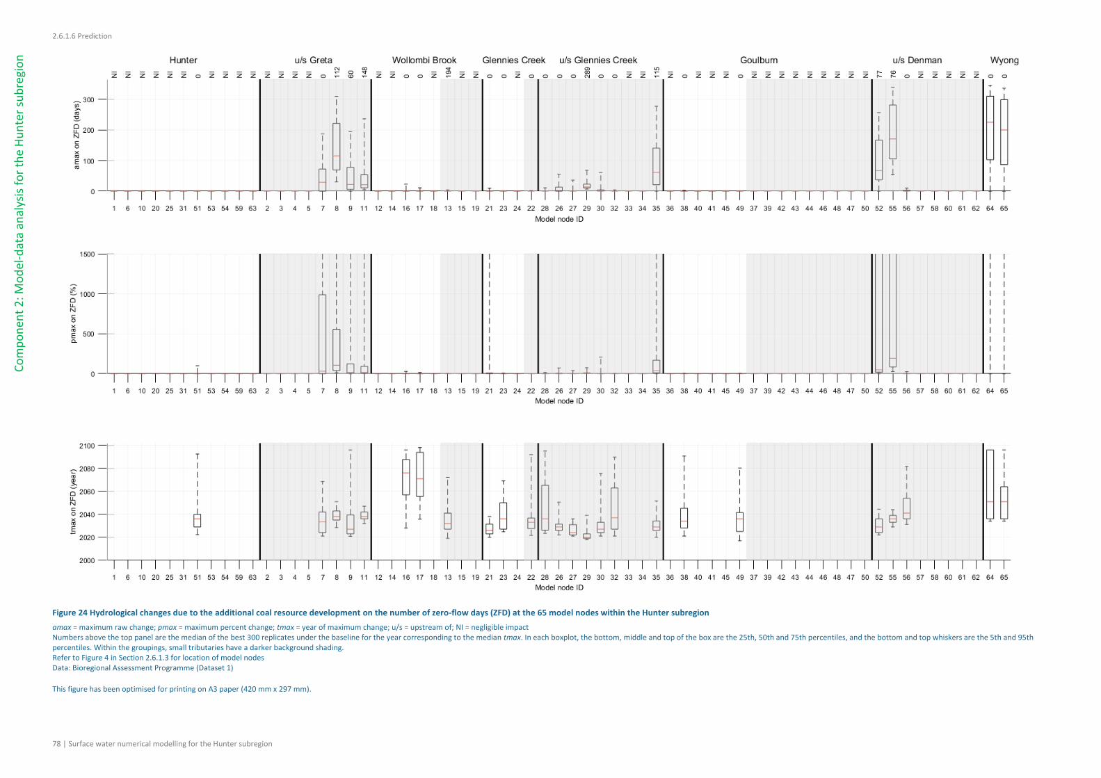
2.6.1.6 Prediction
78 | Surface water numerical modelling for the Hunter subregion
Co
mp
on
ent
2: M
od
el-d
ata
anal
ysis
fo
r th
e H
un
ter
sub
regi
on
Figure 24 Hydrological changes due to the additional coal resource development on the number of zero-flow days (ZFD) at the 65 model nodes within the Hunter subregion
amax = maximum raw change; pmax = maximum percent change; tmax = year of maximum change; u/s = upstream of; NI = negligible impact Numbers above the top panel are the median of the best 300 replicates under the baseline for the year corresponding to the median tmax. In each boxplot, the bottom, middle and top of the box are the 25th, 50th and 75th percentiles, and the bottom and top whiskers are the 5th and 95th percentiles. Within the groupings, small tributaries have a darker background shading. Refer to Figure 4 in Section 2.6.1.3 for location of model nodes Data: Bioregional Assessment Programme (Dataset 1)
This figure has been optimised for printing on A3 paper (420 mm x 297 mm).
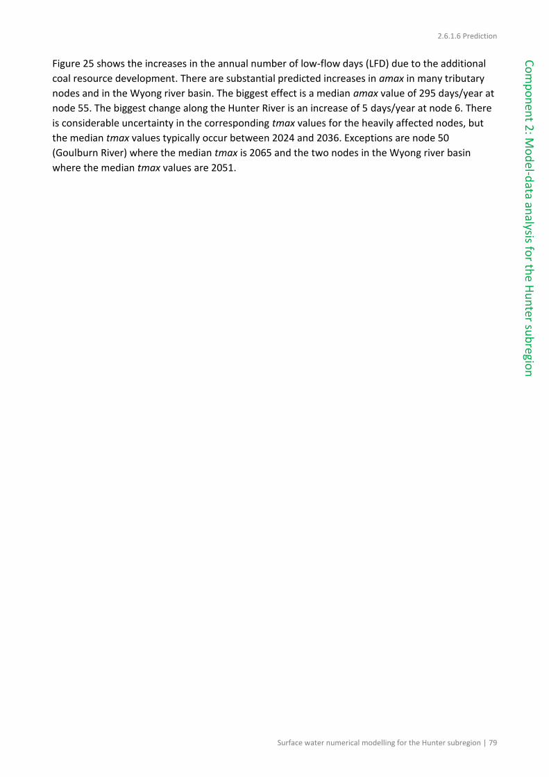
2.6.1.6 Prediction
Surface water numerical modelling for the Hunter subregion | 79
Co
mp
on
ent 2
: Mo
del-d
ata analysis fo
r the
Hu
nter su
bregio
n
Figure 25 shows the increases in the annual number of low-flow days (LFD) due to the additional
coal resource development. There are substantial predicted increases in amax in many tributary
nodes and in the Wyong river basin. The biggest effect is a median amax value of 295 days/year at
node 55. The biggest change along the Hunter River is an increase of 5 days/year at node 6. There
is considerable uncertainty in the corresponding tmax values for the heavily affected nodes, but
the median tmax values typically occur between 2024 and 2036. Exceptions are node 50
(Goulburn River) where the median tmax is 2065 and the two nodes in the Wyong river basin
where the median tmax values are 2051.
2.6.1.6 Prediction
80 | Surface water numerical modelling for the Hunter subregion
Co
mp
on
ent
2: M
od
el-d
ata
anal
ysis
fo
r th
e H
un
ter
sub
regi
on
Figure 25 Hydrological changes due to the additional coal resource development on the number of low-flow days (LFD) at the 65 model nodes within the Hunter subregion
amax = maximum raw change; pmax = maximum percent change; tmax = year of maximum change; u/s = upstream of; NI = negligible impact Numbers above the top panel are the median of the best 300 replicates under the baseline for the year corresponding to the median tmax. In each boxplot, the bottom, middle and top of the box are the 25th, 50th and 75th percentiles, and the bottom and top whiskers are the 5th and 95th percentiles. Within the groupings, small tributaries have a darker background shading. Refer to Figure 4 in Section 2.6.1.3 for location of model nodes. Data: Bioregional Assessment Programme (Dataset 1)
This figure has been optimised for printing on A3 paper (420 mm x 297 mm).

2.6.1.6 Prediction
Surface water numerical modelling for the Hunter subregion | 81
Co
mp
on
ent 2
: Mo
del-d
ata analysis fo
r the
Hu
nter su
bregio
n
Figure 26 shows the changes in low-flow spells (LFS) due to the additional coal resource
development. Increases in median amax of more than three spells per year occur at tributary
nodes 7, 8, 9, 52 and 55 as well as at nodes 64 and 65 in the Wyong river basin. The biggest
changes are increases of 21 spells at nodes 8 and 55. However, there are also substantial increases
in LFS at nodes 10, 20, 25 and 31 along the Hunter River, including a median change of 12 spells at
node 31 (Liddell). Interestingly, there are two small tributary nodes (26 and 29) where median
amax shows a decrease by two spells per year. These reductions in amax result when multiple
spells coalesce into a single large spell.
There is considerable uncertainty in the projections of both amax and tmax in Figure 26.

2.6.1.6 Prediction
82 | Surface water numerical modelling for the Hunter subregion
Co
mp
on
ent
2: M
od
el-d
ata
anal
ysis
fo
r th
e H
un
ter
sub
regi
on
Figure 26 Hydrological changes due to the additional coal resource development on the number of low-flow spells (LFS) at the 65 model nodes within the Hunter subregion
amax = maximum raw change; pmax = maximum percent change; tmax = year of maximum change; u/s = upstream of; NI = negligible impact Numbers above the top panel are the median of the best 300 replicates under the baseline for the year corresponding to the median tmax. In each boxplot, the bottom, middle and top of the box are the 25th, 50th and 75th percentiles, and the bottom and top whiskers are the 5th and 95th percentiles. Within the groupings, small tributaries have a darker background shading. Refer to Figure 4 in Section 2.6.1.3 for location of model nodes. Data: Bioregional Assessment Programme (Dataset 1)
This figure has been optimised for printing on A3 paper (420 mm x 297 mm).

2.6.1.6 Prediction
Surface water numerical modelling for the Hunter subregion | 83
Co
mp
on
ent 2
: Mo
del-d
ata analysis fo
r the
Hu
nter su
bregio
n
Figure 27 shows the maximum changes to the length of the longest low-flow spell (LLFS). The
changes in the LLFS are very similar to those in LFD. The LLFS is projected to increase by about 130
days at node 8 (Doctors Creek) and by more than 15 days at several other small tributary nodes.
The LLFS is projected to increase by 32 and 37 days at the two nodes in the Wyong river basin.

2.6.1.6 Prediction
84 | Surface water numerical modelling for the Hunter subregion
Co
mp
on
ent
2: M
od
el-d
ata
anal
ysis
fo
r th
e H
un
ter
sub
regi
on
Figure 27 Hydrological changes due to the additional coal resource development on the length of longest low-flow spell (LLFS) at the 65 model nodes within the Hunter subregion
amax = maximum raw change; pmax = maximum percent change; tmax = year of maximum change; u/s = upstream of; NI = negligible impact Numbers above the top panel are the median of the best 300 replicates under the baseline for the year corresponding to the median tmax. In each boxplot, the bottom, middle and top of the box are the 25th, 50th and 75th percentiles, and the bottom and top whiskers are the 5th and 95th percentiles. Within the groupings, small tributaries have a darker background shading. Refer to Figure 4 in Section 2.6.1.3 for location of model nodes. Data: Bioregional Assessment Programme (Dataset 1)
This figure has been optimised for printing on A3 paper (420 mm x 297 mm).

2.6.1.6 Prediction
Surface water numerical modelling for the Hunter subregion | 85
Co
mp
on
ent 2
: Mo
del-d
ata analysis fo
r the
Hu
nter su
bregio
n
2.6.1.6.3 Summary and discussion
The prediction results show that the additional coal resource development in the Hunter
subregion can affect all of the hydrological response variables. Comparisons across the 65
model nodes show that the relative hydrological changes are larger for the nodes where the
maximum footprint for the additional coal resource development affects a larger proportion of
the catchment. For instance, the mine footprints in the catchments contributing to nodes 52 and
55 comprise 66% and 58% of the total contributing area, respectively (these areas are reported
in Table 4 in Section 2.6.1.3). The resulting median pmax values for the high-flow flux-based
variables, AF and P99, are around –68% and –59%, respectively. In general the median change
in these variables is highly correlated and commensurate with the maximum proportion of the
catchment that is included in the footprint for the additional coal resource development. Large
changes are also predicted for node 8 for many hydrological response variables (–81% for AF and –
65% for P99). Here the footprint for the additional coal resource development comprises 55% of
the contributing area to this node, but since the node is also heavily affected by mining under the
baseline, even larger hydrological changes are predicted relative to its proportional area.
The prediction results show that the additional coal resource development in the Hunter
subregion has more noticeable effects on hydrological response variables in the small tributaries
of the Hunter River, where the proportion of contributing area affected by mining is more likely to
be high, than at the nodes along the Hunter River itself. This is particularly apparent in streamflow
at nodes 7 to 9 (Loders Creek, including Doctors Creek), which enter the Hunter River just
upstream of Singleton, and at nodes 52 (Dry Creek) and 55 (unnamed creek) in the vicinity of
Muswellbrook. The catchments of nodes 7 to 9 include the Bulga and Mount Thorley–Warkworth
additional coal resource developments, which affect 35–55% of the contributing areas (Table 4
in Section 2.6.1.3); the catchments of nodes 52 and 55 include the Bengalla and Mount Pleasant
mines. Other nodes with substantial percentage changes in the high-streamflow hydrological
response variables are nodes 26, 27, 29 and 35. The first three of these nodes are all located in
the vicinity of the Glendell, Integra, Liddell and Mount Owen mines, while the catchment of node
35 includes parts of the Drayton South and Mount Arthur mines. All these nodes have relatively
small contributing areas. While there are bigger predicted changes in amax at nodes further
downstream, the proportional effects of these changes are diluted by relatively unaffected
inflows. The prediction that the biggest effects occur downstream of multiple mine developments
highlights the cumulative nature of potential hydrological changes, particularly on low-flow
characteristics.
The biggest changes (in terms of amax) on the low-streamflow hydrological response variables are
also predicted to occur at these small tributary nodes. However, unlike for the high-streamflow
hydrological response variables, there is also a substantial change in the low-streamflow
hydrological response variables in the two nodes of the Wyong river basin. These nodes are
located near the proposed Wallarah 2 and Mandalong underground mines. The effect of these
reductions in baseflow is to turn what was previously a perennial stream into one that flows on
only about 40% of days in the most heavily affected year. Although this is a large reduction, it must
be remembered that the projections presented in Figure 19 to Figure 27 are for the worst-case
year during the entire simulation period (2013 to 2102). There is no implication, particularly for
the low-flow variables, that the changes will be this severe in every year.
2.6.1.6 Prediction
86 | Surface water numerical modelling for the Hunter subregion
Co
mp
on
ent
2: M
od
el-d
ata
anal
ysis
fo
r th
e H
un
ter
sub
regi
on
Substantial increases in ZFD would be expected where the river connection with groundwater is
broken – that is, if drawdown causes the watertable in the alluvium to drop below the channel
bed. In such a situation, a perennial or intermittent stream would switch to an ephemeral system,
which by definition only flows in response to rainfall-runoff events. As part of the Hunter
subregion groundwater modelling (companion product 2.6.2 for the Hunter subregion (Herron
et al., 2018b)) hydraulic property information from the Wallarah 2 environmental assessment
(Mackie Environmental Research, 2013) was used to illustrate the process by which local
information can be used to constrain the regional-scale predictions. The parameters from the
environmental assessment indicated relatively poor connectivity through the overburden above
the mine. The simulations informed by lower hydraulic conductivity parameters resulted in
drawdowns towards the lower end of the range of predictions from the regional groundwater
model (see Section 2.6.2.8.4 in Herron et al., 2018b). This suggests that the larger changes in
baseflows from the set of regional groundwater parameters are over-estimates and that the
Wyong River is unlikely to switch to an intermittent flow regime (i.e. a variable connection to
groundwater). This is an area where more detailed investigation is needed to reduce the
uncertainty around these predictions.
The changes due to the additional coal resource development on the low-streamflow hydrological
response variables (P01, LFD, ZFD, LFS and LLFS) appear to be slightly more noticeable than those
on the high-streamflow hydrological response variables (AF, P99 and FD). The flux-based variables
(AF, IQR, P99 and P01) have similar median pmax values at the most heavily affected nodes.
However, of the two frequency-based variables that are most directly comparable – FD and LFD –
the increases in median amax values in the latter are typically larger than the decreases in the
former. However, the uncertainties in predicted pmax (for the flux-based variables), amax (for
the frequency-based variables) and tmax are greater for the low-flow variables.
For high-streamflow hydrological response variables, the tmax at nodes with noticeable changes
occurs approximately when the maximum footprint for the additional coal resource development
occurs. This indicates that the instantaneous streamflow reduction caused by the mine footprint
for the additional coal resource development dominates amax and pmax in these hydrological
response variables while the changes from the cumulative effect on baseflow over time caused
by watertable drawdown are negligible. This conclusion is supported by the tightly constrained
changes in pmax at most nodes which suggest that the biggest effect on the high-streamflow
hydrological response variables is caused by interception and retention of surface runoff at the
mine sites, rather than by reduced baseflow associated with groundwater drawdown.
For low-streamflow hydrological response variables, the tmax at nodes with noticeable changes
does not occur consistently with the time when the maximum footprint for the additional coal
resource development occurs. At many of the most heavily affected nodes, the predicted median
tmax values tend to be a little later for two of the low-streamflow hydrological response variables
– P01 and LLFS. This indicates that the causes of the changes on the low-flow variables are
controlled by a combination of the instantaneous change from the additional mine footprints
and the cumulative effect on baseflow over time caused by watertable drawdown. Therefore, it
is expected that uncertainty in predicting the changes on low-streamflow hydrological response
variables is much larger than that on high-streamflow response variables.

2.6.1.6 Prediction
Surface water numerical modelling for the Hunter subregion | 87
Co
mp
on
ent 2
: Mo
del-d
ata analysis fo
r the
Hu
nter su
bregio
n
2.6.1.6.4 Defining thresholds of hydrological change
The consequences of the changes to streamflow characteristics described in this product on
landscape classes and water-dependent assets are considered in companion product 3-4 for the
Hunter subregion (as listed in Table 2). In order to rule out water-dependent landscape classes and
assets that are unlikely to be impacted by changes in surface water hydrology, it is necessary to
define the magnitude of change in hydrology below which reaches of the stream network are
assumed to experience no significant hydrological change due to the additional coal resource
development. A threshold has been defined conservatively for each of the nine hydrological
response variables in Section 8.1.4 of Viney (2016). For:
the flux-based hydrological response variables AF, P99 and IQR, this is a 5% or greater
chance of a 1% or greater change in the variable (i.e. if at least 5% of model replicates show
a maximum difference between the CRDP and baseline of at least 1% of the baseline value)
the flux-based hydrological response variable P01, this is a 5% or greater chance of a 1% or
greater change in the variable and the change in runoff depth is greater than 0.0002 mm.
Note that the addition of a runoff depth threshold is a departure from Viney (2016) and is
designed to exclude reaches where the absolute change in runoff is negligible.
the frequency-based metrics FD, LFD, LLFS and ZFD, this is a greater than 5% chance of there
being a change in the variable of at least 3 days in any year
the frequency-based metric LFS, this is a greater than 5% chance of there being a change in
the variable of at least two spells in any year.
If results from the surface water modelling indicate that for all nine variables at a model node
there is a less than a 5% probability the hydrological changes will exceed the thresholds, then
landscape classes and assets that depend on streamflow at that location are very unlikely to be
impacted due to the additional coal resource development.
Streams, predicted to experience changes that exceed these thresholds, will not necessarily
be adversely impacted by these changes. Rather they are retained in the group of ‘potentially
impacted’ streams for which more local information and analysis are needed to assess the
implications of the changes on ecological, economic and sociocultural values. Thus these
thresholds form the basis for defining the zone of potential hydrological change (see companion
product 3-4), within which the potential for impacts cannot be ruled out.
Table 11 summarises for each surface water modelling node in the Hunter subregion whether the
hydrological change due to the additional coal resource development exceeds the threshold for
each hydrological response variable. At nodes 2–5, 15, 19, 23–24, 33–34, 39, 57–63, there are no
significant hydrological changes due to the additional coal resource development; at nodes 7–9,
11, 26–27, 29, 35, 52 and 55, changes in all nine hydrological response variables exceed their
respective thresholds; at all other nodes, there are above-threshold changes in some hydrological
response variables, but not others. The last row in Table 11 gives the number of nodes for which
the hydrological response variable was modelled to exceed its specified threshold. The majority of
nodes (46) experience changes in three of the low-streamflow hydrological response variables
(LFD, LFS and LLFS) and in the IQR hydrological response variable (43); less than a third exceed the

2.6.1.6 Prediction
88 | Surface water numerical modelling for the Hunter subregion
Co
mp
on
ent
2: M
od
el-d
ata
anal
ysis
fo
r th
e H
un
ter
sub
regi
on
specified threshold for the ZFD hydrological response variable; about half (33) exceed the specified
threshold for AF.
Table 11 Change in hydrological response variable (column) relative to its threshold at each model node (row) due
to additional coal resource development
AF P99 IQR FD P01 LFD LFS LLFS ZFD
1 ET ET ET ET ET ET ET ET –
2 – – – – – – – – –
3 – – – – – – – – –
4 – – – – – – – – –
5 – – – – – – – – –
6 ET ET ET ET ET ET ET ET –
7 ET ET ET ET ET ET ET ET ET
8 ET ET ET ET ET ET ET ET ET
9 ET ET ET ET ET ET ET ET ET
10 ET ET ET ET – ET ET ET –
11 ET ET ET ET ET ET ET ET ET
12 ET ET ET ET ET ET ET ET –
13 – – ET – – ET ET ET ET
14 ET ET ET ET ET ET ET ET –
15 – – – – – – – – –
16 – ET ET ET ET ET ET ET ET
17 – ET ET ET ET ET ET ET ET
18 – – – – ET ET ET ET –
19 – – – – – – – – –
20 ET ET ET ET – ET ET ET –
21 – ET ET – ET ET ET ET ET
22 ET ET ET ET ET ET ET ET –
23 – – – – – – – – –
24 – – – – – – – – –
25 ET ET ET ET – ET ET ET –
26 ET ET ET ET ET ET ET ET ET
27 ET ET ET ET ET ET ET ET ET
28 – ET ET – ET ET ET ET ET
29 ET ET ET ET ET ET ET ET ET
30 ET – ET ET ET ET ET ET ET
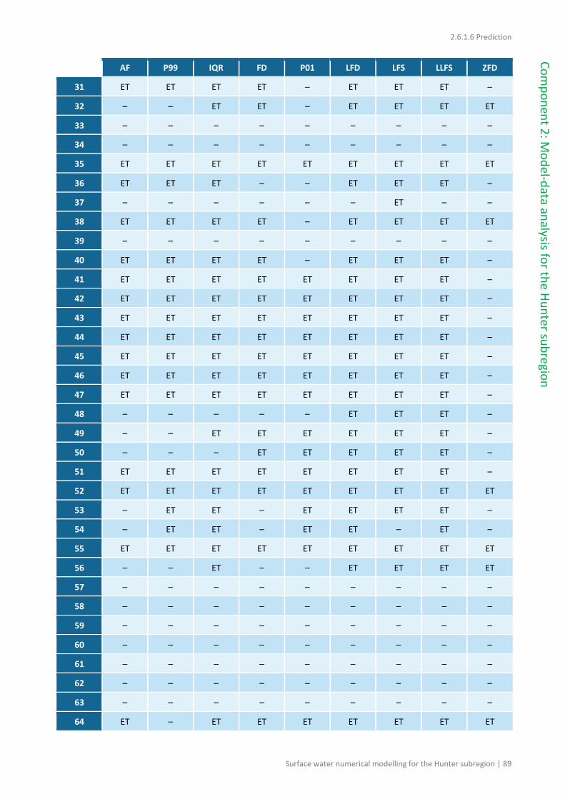
2.6.1.6 Prediction
Surface water numerical modelling for the Hunter subregion | 89
Co
mp
on
ent 2
: Mo
del-d
ata analysis fo
r the H
un
ter sub
region
AF P99 IQR FD P01 LFD LFS LLFS ZFD
31 ET ET ET ET – ET ET ET –
32 – – ET ET – ET ET ET ET
33 – – – – – – – – –
34 – – – – – – – – –
35 ET ET ET ET ET ET ET ET ET
36 ET ET ET – – ET ET ET –
37 – – – – – – ET – –
38 ET ET ET ET – ET ET ET ET
39 – – – – – – – – –
40 ET ET ET ET – ET ET ET –
41 ET ET ET ET ET ET ET ET –
42 ET ET ET ET ET ET ET ET –
43 ET ET ET ET ET ET ET ET –
44 ET ET ET ET ET ET ET ET –
45 ET ET ET ET ET ET ET ET –
46 ET ET ET ET ET ET ET ET –
47 ET ET ET ET ET ET ET ET –
48 – – – – – ET ET ET –
49 – – ET ET ET ET ET ET –
50 – – – ET ET ET ET ET –
51 ET ET ET ET ET ET ET ET –
52 ET ET ET ET ET ET ET ET ET
53 – ET ET – ET ET ET ET –
54 – ET ET – ET ET – ET –
55 ET ET ET ET ET ET ET ET ET
56 – – ET – – ET ET ET ET
57 – – – – – – – – –
58 – – – – – – – – –
59 – – – – – – – – –
60 – – – – – – – – –
61 – – – – – – – – –
62 – – – – – – – – –
63 – – – – – – – – –
64 ET – ET ET ET ET ET ET ET

2.6.1.6 Prediction
90 | Surface water numerical modelling for the Hunter subregion
Co
mp
on
ent
2: M
od
el-d
ata
anal
ysis
fo
r th
e H
un
ter
sub
regi
on
AF P99 IQR FD P01 LFD LFS LLFS ZFD
65 ET – ET ET ET ET ET ET ET
Count 33 36 43 37 35 46 46 46 21
ET = exceeds threshold; – indicates not significant (see Viney (2016) and start of this section for definitions)
In Section 2.1.4.2.5 of companion product 2.1-2.2 for the Hunter subregion (Herron et al., 2018a),
the node to link mapping for the modelled Hunter River and Wyong River networks is defined. This
mapping informs the extrapolation of results from model nodes to some length of reach upstream
and downstream of the node, as appropriate to do so. The information in Table 11 and the node-
link mapping in Section 2.1.4 of Herron et al. (2018a) have been used to identify the reaches of the
Hunter blue line river network (Dataset 3) that have modelled hydrological changes from
additional coal resource development. Figure 28 shows reaches predicted to experience a change
in at least one hydrological response variable above its specified threshold due to additional coal
resource development.
For some reaches (e.g. node 18 to node 19; node 55 to node 59), the change from an above
threshold hydrological change to a non-significant hydrological change occurs somewhere
between the two nodes. These reaches are shown as dashed pink lines and other information is
needed to determine where to delineate the point of change. Similarly, upstream of the pink
headwater model nodes in Figure 28 (i.e. those showing with a change exceeding a specified
hydrological threshold), there will be some length of stream that is also potentially affected by the
additional coal resource development. To define the zone of potential hydrological change for the
impact and risk analysis – that is, the area outside of which it is very unlikely that landscape classes
and assets will be impacted – we need to determine the upstream extents of the stream network
likely to experience a hydrological change exceeding at least one specified threshold. This final
step is reported in companion product 3-4 (impact and risk analysis) for the Hunter subregion (as
listed in Table 2), where drawdown results from the groundwater modelling and mine footprint
data are used to identify stream reaches that are not explicit in the surface water model node-link
network and where hydrological changes from additional coal resource development could impact
water-dependent landscapes and assets.
What these potential changes in hydrology from additional coal resource development might
mean for Hunter subregion landscape classes and assets are covered in companion products
2.7 (receptor impact modelling) and 3-4 (impact and risk analysis) for the Hunter subregion
(as listed in Table 2).
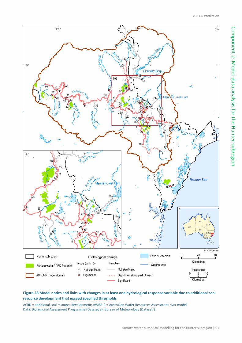
2.6.1.6 Prediction
Surface water numerical modelling for the Hunter subregion | 91
Co
mp
on
ent 2
: Mo
del-d
ata analysis fo
r the H
un
ter sub
region
Figure 28 Model nodes and links with changes in at least one hydrological response variable due to additional coal
resource development that exceed specified thresholds
ACRD = additional coal resource development; AWRA-R = Australian Water Resources Assessment river model Data: Bioregional Assessment Programme (Dataset 2); Bureau of Meteorology (Dataset 3)
2.6.1.6 Prediction
92 | Surface water numerical modelling for the Hunter subregion
Co
mp
on
ent
2: M
od
el-d
ata
anal
ysis
fo
r th
e H
un
ter
sub
regi
on
References
Dawes WR, Herron NF, Macfarlane C, Rachakonda PK, Henderson BL, Ford JH, Wilkes PG,
Marvanek SP, Ramage A (2018) Conceptual modelling for the Hunter subregion. Product 2.3
for the Hunter subregion from the Northern Sydney Basin Bioregional
Assessment. Department of the Environment and Energy, Bureau of Meteorology, CSIRO and
Geoscience Australia, Australia.
http://data.bioregionalassessments.gov.au/product/NSB/HUN/2.3.
Herron NF, Frery E, Crosbie R, Peña-Arancibia J, Zhang YQ, Viney N, Rachakonda PK, Ramage A,
Marvanek SP, Gresham M, McVicar TR, Wilkins A (2018a) Observations analysis, statistical
analysis and interpolation for the Hunter subregion. Product 2.1-2.2 for the Hunter
subregion from the Northern Sydney Basin Bioregional Assessment. Department of the
Environment and Energy, Bureau of Meteorology, CSIRO and Geoscience Australia, Australia.
http://data.bioregionalassessments.gov.au/product/NSB/HUN/2.1-2.2.
Herron NF, Peeters L, Crosbie R, Marvanek SP, Pagendam D, Ramage A, Rachakonda PK and
Wilkins A (2018b) Groundwater modelling for the Hunter subregion. Product 2.6.2 for the
Hunter subregion from the Northern Sydney Basin Bioregional Assessment. Department of
the Environment and Energy, Bureau of Meteorology, CSIRO and Geoscience Australia,
Australia. http://data.bioregionalassessments.gov.au/product/NSB/HUN/2.6.2.
Mackie Environmental Research (2013) Wallarah 2 Coal Project. Groundwater Impact Assessment.
February 2013. Report No M7589/R6. Viewed 16 November 2016,
https://majorprojects.affinitylive.com/public/4af1d9804380abfb6c9412514c24030f/10.%20
Wallarah%202%20Coal%20Project%20EIS%20-%20Appendix%20I%20-
%20Groundwater%20Impact%20Assessment.pdf.
Viney N (2016) Surface water modelling. Submethodology M06 from the Bioregional Assessment
Technical Programme. Department of the Environment and Energy, Bureau of Meteorology,
CSIRO and Geoscience Australia, Australia.
http://data.bioregionalassessments.gov.au/submethodology/M06.
Datasets
Dataset 1 Bioregional Assessment Programme (2016) HUN AWRA-LR Model v01. Bioregional
Assessment Derived Dataset. Viewed 07 December 2016,
http://data.bioregionalassessments.gov.au/dataset/670de516-30c5-4724-bd76-
8ff4a42ca7a5.
Dataset 2 Bioregional Assessment Programme (2017) HUN SW Modelling Reaches and HRV lookup
20170106 v01. Bioregional Assessment Derived Dataset. Viewed 18 January 2017,
http://data.bioregionalassessments.gov.au/dataset/a55000e4-4fb3-49ea-8c1c-
ab6d12750a3e.
2.6.1.6 Prediction
Surface water numerical modelling for the Hunter subregion | 93
Co
mp
on
ent 2
: Mo
del-d
ata analysis fo
r the H
un
ter sub
region
Dataset 3 Bureau of Meteorology (2011) Geofabric Surface Cartography - V2.1. Bioregional
Assessment Source Dataset. Viewed 07 December 2016,
http://data.bioregionalassessments.gov.au/dataset/5342c4ba-f094-4ac5-a65d-
071ff5c642bc.
Glossary
94 | Surface water numerical modelling for the Hunter subregion
Co
mp
on
ent
2: M
od
el-d
ata
anal
ysis
fo
r th
e H
un
ter
sub
regi
on
Glossary
The register of terms and definitions used in the Bioregional Assessment Programme is available
online at http://environment.data.gov.au/def/ba/glossary (note that terms and definitions are
respectively listed under the 'Name' and 'Description' columns in this register). This register is a list
of terms, which are the preferred descriptors for concepts. Other properties are included for each
term, including licence information, source of definition and date of approval. Semantic
relationships (such as hierarchical relationships) are formalised for some terms, as well as linkages
to other terms in related vocabularies.
activity: for the purposes of Impact Modes and Effects Analysis (IMEA), a planned event associated
with a coal seam gas (CSG) operation or coal mine. For example, activities during the production
life-cycle stage in a CSG operation include drilling and coring, ground-based geophysics and
surface core testing. Activities are grouped into components, which are grouped into life-cycle
stages.
additional coal resource development: all coal mines and coal seam gas (CSG) fields, including
expansions of baseline operations, that are expected to begin commercial production after
December 2012
asset: an entity that has value to the community and, for bioregional assessment purposes, is
associated with a subregion or bioregion. Technically, an asset is a store of value and may be
managed and/or used to maintain and/or produce further value. Each asset will have many values
associated with it and they can be measured from a range of perspectives; for example, the values
of a wetland can be measured from ecological, sociocultural and economic perspectives.
baseline coal resource development: a future that includes all coal mines and coal seam gas (CSG)
fields that are commercially producing as of December 2012
bioregion: a geographic land area within which coal seam gas (CSG) and/or coal mining
developments are taking place, or could take place, and for which bioregional assessments (BAs)
are conducted
bioregional assessment: a scientific analysis of the ecology, hydrology, geology and hydrogeology
of a bioregion, with explicit assessment of the potential direct, indirect and cumulative impacts of
coal seam gas and coal mining development on water resources. The central purpose of
bioregional assessments is to analyse the impacts and risks associated with changes to water-
dependent assets that arise in response to current and future pathways of coal seam gas and coal
mining development.
coal resource development pathway: a future that includes all coal mines and coal seam gas (CSG)
fields that are in the baseline as well as those that are expected to begin commercial production
after December 2012
conceptual model: abstraction or simplification of reality
connectivity: a descriptive measure of the interaction between water bodies (groundwater and/or
surface water)

Glossary
Surface water numerical modelling for the Hunter subregion | 95
Co
mp
on
ent 2
: Mo
del-d
ata analysis fo
r the
Hu
nter su
bregio
n
consequence: synonym of impact
context: the circumstances that form the setting for an event, statement or idea
cumulative impact: for the purposes of bioregional assessments, the total change in water
resources and water-dependent assets resulting from coal seam gas and coal mining
developments when all past, present and reasonably foreseeable actions that are likely to impact
on water resources are considered
dataset: a collection of data in files, in databases or delivered by services that comprise a related
set of information. Datasets may be spatial (e.g. a shape file or geodatabase or a Web Feature
Service) or aspatial (e.g. an Access database, a list of people or a model configuration file).
discharge: water that moves from a groundwater body to the ground surface or surface water
body (e.g. a river or lake)
diversion: see extraction
drawdown: a lowering of the groundwater level (caused, for example, by pumping). In the
bioregional assessment (BA) context this is reported as the difference in groundwater level
between two potential futures considered in BAs: baseline coal resource development (baseline)
and the coal resource development pathway (CRDP). The difference in drawdown between CRDP
and baseline is due to the additional coal resource development (ACRD). Drawdown under the
baseline is relative to drawdown with no coal resource development; likewise, drawdown under
the CRDP is relative to drawdown with no coal resource development.
effect: for the purposes of Impact Modes and Effects Analysis (IMEA), change in the quantity
and/or quality of surface water or groundwater. An effect is a specific type of an impact (any
change resulting from prior events).
extraction: the removal of water for use from waterways or aquifers (including storages) by
pumping or gravity channels
formation: rock layers that have common physical characteristics (lithology) deposited during a
specific period of geological time
Geofabric: a nationally consistent series of interrelated spatial datasets defining hierarchically-
nested river basins, stream segments, hydrological networks and associated cartography
groundwater: water occurring naturally below ground level (whether in an aquifer or other low
permeability material), or water occurring at a place below ground that has been pumped,
diverted or released to that place for storage there. This does not include water held in
underground tanks, pipes or other works.
Hunter subregion: Along the coast, the Hunter subregion extends north from the northern edge of
Broken Bay on the New South Wales Central Coast to just north of Newcastle. The subregion is
bordered in the west and north–west by the Great Dividing Range and in the north by the towns of
Scone and Muswellbrook. The Hunter River is the major river in the subregion, rising in the
Barrington Tops and Liverpool Ranges and draining south‑west to Lake Glenbawn before heading

Glossary
96 | Surface water numerical modelling for the Hunter subregion
Co
mp
on
ent
2: M
od
el-d
ata
anal
ysis
fo
r th
e H
un
ter
sub
regi
on
east where it enters the Tasman Sea at Newcastle. The subregion also includes smaller catchments
along the central coast, including the Macquarie and Tuggerah lakes catchments.
hydrogeology: the study of groundwater, including flow in aquifers, groundwater resource
evaluation, and the chemistry of interactions between water and rock
hydrological response variable: a hydrological characteristic of the system that potentially changes
due to coal resource development (for example, drawdown or the annual streamflow volume)
impact: a change resulting from prior events, at any stage in a chain of events or a causal pathway.
An impact might be equivalent to an effect (change in the quality and/or quantity of surface water
or groundwater), or it might be a change resulting from those effects (for example, ecological
changes that result from hydrological changes).
impact mode: the manner in which a hazardous chain of events (initiated by an impact cause)
could result in an effect (change in the quality and/or quantity of surface water or groundwater).
There might be multiple impact modes for each activity or chain of events.
inflow: surface water runoff and deep drainage to groundwater (groundwater recharge) and
transfers into the water system (both surface water and groundwater) for a defined area
landscape class: for bioregional assessment (BA) purposes, an ecosystem with characteristics that
are expected to respond similarly to changes in groundwater and/or surface water due to coal
resource development. Note that there is expected to be less heterogeneity in the response within
a landscape class than between landscape classes. They are present on the landscape across the
entire BA subregion or bioregion and their spatial coverage is exhaustive and non-overlapping.
Conceptually, landscape classes can be considered as types of ecosystem assets.
model node: a point in the landscape where hydrological changes (and their uncertainty) are
assessed. Hydrological changes at points other than model nodes are obtained by interpolation.
porosity: the proportion of the volume of rock consisting of pores, usually expressed as a
percentage of the total rock or soil mass
receptor: a point in the landscape where water-related impacts on assets are assessed
risk: the effect of uncertainty on objectives
runoff: rainfall that does not infiltrate the ground or evaporate to the atmosphere. This water
flows down a slope and enters surface water systems.
sensitivity: the degree to which the output of a model (numerical or otherwise) responds to
uncertainty in a model input
source dataset: a pre-existing dataset sourced from outside the Bioregional Assessment
Programme (including from Programme partner organisations) or a dataset created by the
Programme based on analyses conducted by the Programme for use in the bioregional
assessments (BAs)
Glossary
Surface water numerical modelling for the Hunter subregion | 97
Co
mp
on
ent 2
: Mo
del-d
ata analysis fo
r the
Hu
nter su
bregio
n
spring: a naturally occurring discharge of groundwater flowing out of the ground, often forming a
small stream or pool of water. Typically, it represents the point at which the watertable intersects
ground level.
subregion: an identified area wholly contained within a bioregion that enables convenient
presentation of outputs of a bioregional assessment (BA)
subsidence: localised lowering of the land surface. It occurs when underground voids or cavities
collapse, or when soil or geological formations (including coal seams, sandstone and other
sedimentary strata) compact due to reduction in moisture content and pressure within the
ground.
surface water: water that flows over land and in watercourses or artificial channels and can be
captured, stored and supplemented from dams and reservoirs
uncertainty: the state, even partial, of deficiency of information related to understanding or
knowledge of an event, its consequence, or likelihood. For the purposes of bioregional
assessments, uncertainty includes: the variation caused by natural fluctuations or heterogeneity;
the incomplete knowledge or understanding of the system under consideration; and the
simplification or abstraction of the system in the conceptual and numerical models.
water allocation: the specific volume of water allocated to water access entitlements in a given
season, defined according to rules established in the relevant water plan
water-dependent asset: an asset potentially impacted, either positively or negatively, by changes
in the groundwater and/or surface water regime due to coal resource development
water use: the volume of water diverted from a stream, extracted from groundwater, or
transferred to another area for use. It is not representative of 'on-farm' or 'town' use; rather it
represents the volume taken from the environment.
watertable: the upper surface of a body of groundwater occurring in an unconfined aquifer. At the
watertable, pore water pressure equals atmospheric pressure.
well: typically a narrow diameter hole drilled into the earth for the purposes of exploring,
evaluating or recovering various natural resources, such as hydrocarbons (oil and gas) or water. As
part of the drilling and construction process the well can be encased by materials such as steel and
cement, or it may be uncased. Wells are sometimes known as a ‘wellbore’.

98 | Surface water numerical modelling for the Hunter subregion
www.bioregionalassessments.gov.au