Surface Roughness Prediction in Machining of Cast Polyamide
6
ORIGINAL ARTICLE Surface roughness prediction in machining of cast polyamide using neural network Serhat Yilmaz • A. Armagan Arici • Erol Feyzullahoglu Recei ved: 22 July 200 9 / Acce pted : 7 Februar y 201 1 Ó Springer-Verlag London Limited 2011 Abstract This pa per is about pr edictin g the surf ace roughness by means of neural network approach method on mac hini ng of an engine eri ng pla stic material. The wor k mat eri al was an ext rud ed PA6 G cas t pol yamide for the machining tests. The network has 2 inputs called spindle speed and feed rate for this study. Output of the network is sur fac e roughn ess (Ra). Gra dient Des cent Met hod was applied to optimize the weight parameters of neuron con- nec tions. The minimum Ra is obt ained for 400 rpm and 251 cm/min as 0.8371 lm. Keywords Surface roughness Á Machining Á Neural network Á Cast polyamide 1 Introd uction Machining processes are used to shape plastics in the case of accurate shapes, complex parts, or for small production volumes, where extrusion and molding are not cost-effec- tive, or for a pr oduct that needs a cost ly di mensiona l accuracy, such as polymer lenses [1, 3]. Turning, milling and grinding are the conventional machining processes and the cutting mechanism is mainly shearing of the material ahead of the cuttin g wedge, resulting in chip forma tion [ 2]. One of the factors that influence the quality of a machined component is associated with the tool design and machining conditions such as rake angle, tip radius, depth of cut and cutting speed [3, 4]. Surface finish is an important param- eter in the machining process. In machining of parts, surface qualit y is one of the most specified custome r requir ements. Major indication of surface quality on machined parts is surface roughness. It has formed an important design fea- ture in many situations such as parts subjected to fatigue loads, precision fits, fastener holes, and aesthetic require- ments. In additi on to tolera nce, surface roughness imposes one of the most cri tic al constra ints for the selec tion of machines and cutting parameters in the process planning [5]. So, surface roughness is an important measure of the technological quality of a product and a factor that greatly influences manufacturing cost [ 2, 3]. Cast pol yamides ser ve as a replac eme nt for bronze, brass, aluminum or steel parts, including rollers and guides, bushings and bearings, gears and sprockets, sheaves and idl ers due to dry-sl idi ng proper ties . The y cover a wid e range of proper tie s and app lic atio ns due to flex ibl e for - mulation, shaping and processing [6]. Neu ral net wor ks (NN) are comput ati ona l int elli gen t methods, whi ch cou ld est ablish a map ping thr ough the numerical inputs and outputs. The NN extract a sensitive, exact and realistic relation from some experimental input– out put data, called traini ng set. In this way , the y cou ld interpolate synthetic data which estimate the results of the exp eri ment s tha t hav e not bee n est abl ishe d, and pre dict optimu m reasonable proces sing condit ions [ 7]. Caydas and Hascalik [9] developed a NN and regression model to predict surface roughness in an abrasive water jet mac hini ng pro cess. The y mac hined AA 7075 aluminum al loy [9]. Dh ok ia et al . [10] pa id attenti on to a li ttl e research that is evident in the literature on the analysis of opt ima l mac hining par ame ter s for mac hining mat eri als S. Yilmaz (&) Electronics and Telecommunications Engineering Department, University of Kocaeli, 41040 Kocaeli, Turkey e-mail: serhatyilmaz@ieee.org A. A. Arici Á E. Feyzullahoglu Mechanical Engineering Department, University of Kocaeli, 41040 Kocaeli, Turkey 123 Neural Comput & Applic DOI 10.1007/s00521-011-0557-y
-
Upload
vaalgatamilram -
Category
Documents
-
view
228 -
download
0
Transcript of Surface Roughness Prediction in Machining of Cast Polyamide

8/3/2019 Surface Roughness Prediction in Machining of Cast Polyamide
http://slidepdf.com/reader/full/surface-roughness-prediction-in-machining-of-cast-polyamide 1/6
O R I G I N A L A R T I C L E
Surface roughness prediction in machining of cast polyamideusing neural network
Serhat Yilmaz • A. Armagan Arici •
Erol Feyzullahoglu
Received: 22 July 2009 / Accepted: 7 February 2011
Ó Springer-Verlag London Limited 2011
Abstract This paper is about predicting the surface
roughness by means of neural network approach method onmachining of an engineering plastic material. The work
material was an extruded PA6G cast polyamide for the
machining tests. The network has 2 inputs called spindle
speed and feed rate for this study. Output of the network is
surface roughness (Ra). Gradient Descent Method was
applied to optimize the weight parameters of neuron con-
nections. The minimum Ra is obtained for 400 rpm and
251 cm/min as 0.8371 lm.
Keywords Surface roughness Á Machining ÁNeural network Á Cast polyamide
1 Introduction
Machining processes are used to shape plastics in the case
of accurate shapes, complex parts, or for small production
volumes, where extrusion and molding are not cost-effec-
tive, or for a product that needs a costly dimensional
accuracy, such as polymer lenses [1, 3]. Turning, milling
and grinding are the conventional machining processes and
the cutting mechanism is mainly shearing of the material
ahead of the cutting wedge, resulting in chip formation [2].
One of the factors that influence the quality of a machined
component is associated with the tool design and machining
conditions such as rake angle, tip radius, depth of cut andcutting speed [3, 4]. Surface finish is an important param-
eter in the machining process. In machining of parts, surface
quality is one of the most specified customer requirements.
Major indication of surface quality on machined parts is
surface roughness. It has formed an important design fea-
ture in many situations such as parts subjected to fatigue
loads, precision fits, fastener holes, and aesthetic require-
ments. In addition to tolerance, surface roughness imposes
one of the most critical constraints for the selection of
machines and cutting parameters in the process planning
[5]. So, surface roughness is an important measure of the
technological quality of a product and a factor that greatly
influences manufacturing cost [2, 3].
Cast polyamides serve as a replacement for bronze,
brass, aluminum or steel parts, including rollers and guides,
bushings and bearings, gears and sprockets, sheaves and
idlers due to dry-sliding properties. They cover a wide
range of properties and applications due to flexible for-
mulation, shaping and processing [6].
Neural networks (NN) are computational intelligent
methods, which could establish a mapping through the
numerical inputs and outputs. The NN extract a sensitive,
exact and realistic relation from some experimental input–
output data, called training set. In this way, they could
interpolate synthetic data which estimate the results of the
experiments that have not been established, and predict
optimum reasonable processing conditions [7].
Caydas and Hascalik [9] developed a NN and regression
model to predict surface roughness in an abrasive water jet
machining process. They machined AA 7075 aluminum
alloy [9]. Dhokia et al. [10] paid attention to a little
research that is evident in the literature on the analysis of
optimal machining parameters for machining materials
S. Yilmaz (&)
Electronics and Telecommunications Engineering Department,
University of Kocaeli, 41040 Kocaeli, Turkey
e-mail: [email protected]
A. A. Arici Á E. Feyzullahoglu
Mechanical Engineering Department, University of Kocaeli,
41040 Kocaeli, Turkey
123
Neural Comput & Applic
DOI 10.1007/s00521-011-0557-y

8/3/2019 Surface Roughness Prediction in Machining of Cast Polyamide
http://slidepdf.com/reader/full/surface-roughness-prediction-in-machining-of-cast-polyamide 2/6
such as polypropylene. They developed a performance
predictive NN model based on surface roughness for
polypropylene machining. In their study, extensive exper-
imental work on different network topologies and training
algorithms has been performed to predict the behavior of
the surface roughness for machined polypropylene prod-
ucts [10]. Basheer et al. [11] proposed an experimental
work on the analysis of machined surface quality on Al/ SiCp composites leading to an ANN (artificial neural net-
work) model to estimate surface roughness whose results
were found to be in a very good agreement with the
unexposed experimental data set [11]. Arafeh and Singh
[12] announced the requirement of new and powerful
paradigms such as NN, fuzzy and neuro-fuzzy approaches
on material processing.
Surface roughness depends on different machining
parameters and its prediction and control is a challenge to
the research. Owing to advances in computing power, there
is an increase in the demand for the use of the intelligent
techniques. Recent researches are directed toward hybrid-ization of intelligent techniques to make best out of each
method. For example Jesuthanam et al. [13] proposed a
hybrid NN trained with Genetic Algorithm (GA) and Par-
ticles Swarm Optimization (PSO) for the prediction of
surface roughness [13].
This paper is about predicting the surface roughness
with neural network approach method on machining of
an engineering plastic material. The spindle speed and
feed rate were the cutting parameters and the quality of
the cutting surfaces was controlled with surface rough-
ness. In this study, a feed-forward NN, which includes
two hidden layers were used. Gradient Descent method
was applied to optimize the weight parameters of neuron
connections.
2 Experimental study
The work material was an extruded PA6G cast polyamide
for the machining tests. The mechanical and thermal
properties of the material are given in Table 1. The milling
experimentations were carried out in 80 mm width and
400 mm length work-pieces using a high-speed-steel
(HSS) four-flute end-milling cutter with a diameter of
12 mm, and the cutting length was 80 mm. Dry-cutting
conditions are maintained for all milling experimentations.
Two cutting parameters were spindle speed (100, 125, 160,
200, 315, 500, 630, 800, 1,000, 1,250, 1,600, 2,000 rpm)
and feed rate (12.5, 25, 40, 50, 80, 100, 125, 200, 315,
400 cm/min) where depth of cut was fixed to 2 mm. The
surface roughnesses were measured on each milled sur-
faces at the fixed positions with Mitutoyo SJ-301 profi-
lometer and the average surface roughness (Ra) was taken.
3 Neural networks model
Predictive models can provide a predictive control by
enabling us to anticipate how process will respond to
changing variables. Dhokia et al. [10] developed a NN
model, which mainly hinges three independent variables
namely spindle speed, feed rate and dept of cut [10].
In this study, NN was used as an input–output fitter
which predicts the relative surface between inputs and
output, by means of calculating the interpolation coeffi-
cients, called weights.These weights constitute a parameter matrix that maps an
equation vector, for example, outputs to a state vector and
inputs in Fig. 1, where SS, FR and Ra are spindle speed,
feed rate and average surface roughness, respectively.
Weights that were given in Fig. 1 are updated according
to the back propagation method which is an adaptation of
gradient descent method to neural networks. The gradient
descent method minimizes error cost function given in
Eq. 1 (Moon and Stirling 1999).
C ¼1
2
Xnk þ1
i¼1
ðd i À yiÞ2 ð1Þ
where d i are desired output values of Ra given in the
training data and yi are the actual ANN output estimations
about Ra given in Fig. 1.
Weights are updated according to Eq. 2.
Dw ¼ Àa rw C ð2Þ
Table 1 Mechanical- and thermal-properties of cast polyamide
Tensile strength 85 MPa
Tensile modulus 4,000 MPa
Charpy impact resistance Without fracture
Hardness (Shore D) 84
Melting temperature 220°C
Coefficient of thermal expansion 89
10
-5°
C
-1
Ra
Input Layer Hidden Layer Output Layer
SS
FR
weights
weights
weights
Fig. 1 Structure of the feed forward NN used for roughness
estimation
Neural Comput & Applic
123

8/3/2019 Surface Roughness Prediction in Machining of Cast Polyamide
http://slidepdf.com/reader/full/surface-roughness-prediction-in-machining-of-cast-polyamide 3/6
where w symbolizes the connection weight and rw means,
partial derivation of a function according to parameter
w. The weight update equation will be:
w‘þ1ij ¼ w‘
ij þ Dw‘
ij ð3Þ
Layers are shown in Fig. 1. i symbolizes the ith neuron
in an antecedent layer where j symbolizes the jth neighbor
neuron of the successor layer. wij is connection weight
between these neurons.
Training, testing and graphing programs of the neural
networks mentioned above was written in Matlab’s pro-
gramming language [8]. The programs are described with
algorithms in ‘‘Appendix’’.
3.1 Training process
The network has two inputs called spindle speed (SS)
(rpm) and feed rate (FR) (cm/min). Output of the network
is surface roughness (Ra) (lm). The Input Layer Neurons
acts as buffers, which transfers the inputs to their outputs,
without any change. The following layers and their
parameters are given in Table 2.
Number and type of the neurons in the hidden layers as
well as the number of hidden layers are determined after
several tries and faults.
Experimental data obtained from the machining processare shared into two sections; for training the network and
then testing it by means of a data set which is unknown for
the trained network (see Figs. 5, 6, 7 in ‘‘Appendix’’).
As an example, first 8 of the 36 training inputs–output
couples are given in Table 3.
However, since the neural network could not estimate
instantaneous changes in the raw data given in the training
and the testing sets, both data sets are scaled due to loga-
rithms of the inputs–output couples. Following the loga-
rithmic scaling, training and testing; stages are processed.
Then, the results of the network are rescaled by means of calculating their exponential values.
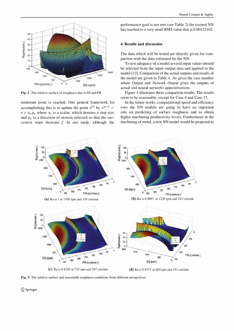
3.2 Testing process and relation surfaces
Relation surfaces are three dimensional graphs which
illustrate the relation between inputs and outputs of a
model. Changes of roughness (Ra) due to the current SS
and FR are shown in Fig. 2. The surface in the figure shows
the testing responses of the trained Neural Networks to
several input combinations; that is, 5,929 iterative simu-
lations (tests) have done to get this response surface.
As seen in the Fig. 2, the relation between the inputs andthe output has a very nonlinear and complex behavior. This
is originated from nature of the machining process, such as
melting of the material over some speed. However, the
surface reasonably proves both training and testing data.
This means, the trained network could not only be used for
estimations of roughness in several processing situations,
but also to predict the optimum roughness condition or
conditions.
Several reasonable roughness conditions are determined
and their corresponding minimum roughness values are
emphasized with arrows in Fig. 3. The white curve shows
the region of minima in the surface (Fig. 3a).
The optimum working region clearly seen in Fig. 3
gives the best surface roughness. The minimum Ra is
obtained for 400 rpm and 251 cm/min as 0.8371 lm.
3.3 Training performance of the neural network used
in surface roughness
Least mean square (LMS) algorithm is used to compute the
training performance of the neural networks [16]. Cost
function as shown in Fig. 4 which is a root mean square of
neural network output errors, is forced to minimize. The
algorithm uses the steepest descent method for minimizing
the function [15]. The method iterates in such a way that
f ð x½nþ1Þ\ f ð x½nÞ unless f ð x½nþ1Þ ¼ f ð x½nÞ in which case a
Table 2 Parameters of the network used for roughness estimation
Number of hidden layers 2
Number of neurons in the 1st hidden layer 3
Type of the transfer functions in the 1st
H.L.
Logarithmic sigmoid
Number of neurons in the 2nd hidden
layer
4
Type of the transfer functions in the 2ndH.L.
Hyperbolic tangentsigmoid
Number of neurons in the output layer 1
Type of the transfer functions in the O.L. Linear
Maximum epochs given in the program 40,000 iterations
Goal of NN’s maximum RMS error
tolerance
1 9 10-6
Reached RMS error value after the
training
0.00122102
Table 3 Training data
SS 100 125 160 160 200 200 200 315 – –
FR 50 50 12.5 25 12.5 80 100 50 – –
Ra 16.3 15.59 5.49 6.42 2.495 4.185 3.16 6.15 – –
Neural Comput & Applic
123
8/3/2019 Surface Roughness Prediction in Machining of Cast Polyamide
http://slidepdf.com/reader/full/surface-roughness-prediction-in-machining-of-cast-polyamide 4/6
minimum point is reached. One general framework for
accomplishing this is to update the point x[n] by x nþ1½ ¼
x þ an: pn where an is a scalar, which denotes a step size
and pn is a direction of motion selected so that the suc-
cessive steps decrease f . In our study, although the
performance goal is not met (see Table 2) the trained NN
has reached to a very small RMS value that is 0.00122102.
4 Results and discussion
The data which will be tested are directly given for com-
parison with the data estimated by the NN.To test adequacy of a model several input values should
be selected from the input–output data and applied to the
model [12]. Comparison of the actual outputs and results of
the model are given in Table 4. No gives the case number
where Output and Network Output gives the outputs of
actual and neural networks approximations.
Figure 4 illustrates these comparison results. The results
seem to be reasonable, except for Case 4 and Case 15.
In the future works, computational speed and efficiency
over the NN models are going to have an important
role on predicting of surface roughness and to obtain
higher machining productivity levels. Furthermore in themachining of metal, a new NN model would be proposed to
0
500
1000
1500
2000
0
100
200
300
4000
10
20
30
40
50
60
SS-(rpm)FR-(cm/min.)
R a ( m i c r o m . )
Fig. 2 The relative surface of roughness due to SS and FR
(a) Ra is 1 at 1700 rpm and 195 cm/min (b) Ra is 0.9067 at 1225 rpm and 183 cm/min
(c) Ra is 0.8385 at 725 rpm and 207 cm/min (d) Ra is 0.8371 at 400 rpm and 251 cm/min
Fig. 3 The relative surface and reasonable roughness conditions from different perspectives
Neural Comput & Applic
123

8/3/2019 Surface Roughness Prediction in Machining of Cast Polyamide
http://slidepdf.com/reader/full/surface-roughness-prediction-in-machining-of-cast-polyamide 5/6
predict surface roughness and tool wear over the machining
time for a variety of cutting conditions in finish hard
turnings [14].
5 Conclusions
Surface roughness is an important outcome to attain higher
productivity levels in the machining process. In this study,a neural network based estimation model is developed in
order to predict the surface roughness appeared in the
machining process of cast polyamide material. Training
performance of the model reached to RMS value of
0.00122102.
Estimated data of the model are obtained similar to the
test data. Due to the roughness surface created by the
model, optimum Ra value is reached to 0.8371 lm at
400 rpm and 251 cm/min.
Acknowledgments The authors thank to Dr. Onder Ekinci and Dr.
Melih Inal for their valuable contributions.
Appendix
See Figs. 5, 6, 7.
-10
0
10
20
30
40
50
60
70
0 2 4 6 8 10 12 14 16
Test Data
NN Outputs
R a ( µ m )
Data No
Fig. 4 Illustrative graphics of testing and estimated data comparison
Table 4 Comparison of testing data and the data estimated by the
trained NN
Input 1 Input 2 Output Network output
No SS FR Ra (Actual) Ra (NN)
1 160 40 10.785 14.09435538
2 160 50 13.92 11.656081963 200 25 4.27 3.569734741
4 315 250 2.39 15.40493881
5 630 50 3.34 2.621217919
6 630 100 3.21 3.140015617
7 630 315 2.44 2.567393269
8 800 80 3.455 2.944766564
9 1,000 80 4.58 3.117496995
10 1,000 200 33.87 32.29606974
11 1,000 315 52.17 34.58952426
12 1,000 400 55.5 54.46757443
13 1,250 80 5.94 3.569225516
14 1,600 125 5.77 3.915849364
15 2,000 125 11.6 2.474200905
Define a neural network called as RoughessEstimatorDetermine
• Ranges of the network inputs
• Number of neurons in the hidden layers and number of
outputs• Types of transfer functions of the neurons in the
hidden layers and in the output layer, respectively
Load experimental data vectorsof inputs (SS and FR) and
output (Ra) in terms of Logaritmic Scale
Rescale input and output vectors due to themaximum values of these variables
Training Stage
• Determine training parameters such as
maximum training epochs, sum squared error
tolerance of the network ….
• Train the network by means of the rescaled
network inputs
• Assign the trained network to a variable calledtrained network
Save the trained network to a file
Fig. 5 Algorithm of the training program
Load testing data vectors of inputs (SS and FR) and
output (Ra)
Rescale testing inputs and output vectors due tothe extremum values of these variables
Testing Stage
• Create an empty output vector
• Simulate the network by means of the test inputs
, read the response of the network
• Fill the output vector with these simulation
results
• Rescale the network outputs to obtain Ra vector
Load the Trained Network
Fig. 6 Algorithm of the performance-testing program
Neural Comput & Applic
123

8/3/2019 Surface Roughness Prediction in Machining of Cast Polyamide
http://slidepdf.com/reader/full/surface-roughness-prediction-in-machining-of-cast-polyamide 6/6
References
1. Brunette J, Jeu-Herault M, Songmene V, Masounave J (2004)
Understanding and characterizing the drilling of recycled plastics.
Mach Sci Technol 8(1):141–170
2. Davim JP, Silva LR, Festas A, Abrao AM (2009) Machinability
study on precision turning of PA66 polyamide with and without
glass fiber reinforcing. Mater Des 30:228–234
3. Xiao KQ, Zhang LC (2002) The role of viscous deformation in
the machining of polymers. Int J Mech Sci 44:2317–2336
4. Mata F, Gaitonde VN, Karnik SR, Davim JP (2009) Influence of
cutting conditions on machinability aspects of PEEK, PEEK CF
30 and PEEK GF 30 composites. J Mater process Technol
209:1980–1987
5. Palanikumar K, Karunamoorthy L, Manoharan N (2006) Math-
ematical model to predict the surface roughness on the machining
of glass fiber reinforced polymer composites. J Reinf Plastics
Compos 25(4):407–419
6. Samyn P, Tuzolana TM (2007) Effect of test scale on the friction
properties of pure and internal-lubricated cast polyamides at
running-in. Polym Test 26:660–675
7. Bose NK, Liang P (1996) Neural network fundamentals with
graphs algorithms and applications. McGraw-Hill, NY
8. http://www.mathworks.com
9. Caydas U, Hascalik A (2008) A study on surface roughness in
abrasive water-jet machining process using artificial neural net-
works and regression analysis method. J Mater Process Technol
202(1–3):574–582
10. Dhokia VG, Kumar S, Vichare P, Newman ST, Allen RD (2008)
Surface roughness prediction model for CNC machining of
polypropylene. Proc Inst Mech Eng Part B J Eng Manuf
222(2):137–153
11. Basheer AC, Dabade UA, Joshi SS, Bhanuprasad VV, Gadre VM
(2008) Modeling of surface roughness in precision machining of
metal matrix composites using ANN. J Mate Process Technol
197(1–3):439–444
12. Arafeh L, Singh H (1999) A neuro fuzzy logic approach to
material processing. IEEE Trans Syst Man Cybern Part C Appl
Rev 29(3):362–370
13. Jesuthanam CP, Kumanan S, Asokan P (2007) Surface roughness
prediction using hybrid neural networks. Mach Sci Technol
11(2):271–286
14. Ozel T, Karpat Y (2005) Predictive modeling of surface rough-
ness and tool wear in hard turning using regression and neural
networks. Int J Mach Tools Manuf 45(4–5):467–479
15. Moon TK, Stirling WC (2000) Mathematical methods and algo-
rithms for signals processing. Prencite-Hall, New Jersey
16. Kosko B (1992) Neural networks and fuzzy systems. Prentice-
Hall, USA
Showing the Results
• Derive the X, Ymeshgrid input axises inmatrix forms from the input vectors.
• Plot the surface which describes output, Z,matrix due to X,Y
• Label the axises and show the surface
• Determine the SS and FR vectors as x and y axises of the Surface
• Rescale the input vectors due to the extremum values of these
variables
Simulation Stage
• Use SS and FR input combinations with two “for-endloops” placing one inside the other, respectively.
• Simulate the network iteratively, by means of these
input combinations. Read the response of the network.
• Write these responses to the NN output vector,
• Rescale the network outputs to obtain Ra vector
Load the Trained Network
Fig. 7 Algorithm of the surface-graphing program
Neural Comput & Applic
123