Surface Reconstruction from Noisy Point Cloudsamenta/pubs/boris.pdf · B. Mederos & N. Amenta & L....

Eurographics Symposium on Geometry Processing (2005)M. Desbrun, H. Pottmann (Editors)

Surface Reconstruction from Noisy Point Clouds

Boris Mederos, Nina Amenta, Luiz Velho and Luiz Henrique de Figueiredo

University of California at DavisIMPA - Instituto Nacional de Matematica Pura e Aplicada

AbstractWe show that a simple modification of the power crust algorithm for surface reconstruction produces correctoutputs in presence of noise. This is proved using a fairly realistic noise model. Our theoretical results are relatedto the problem of computing a stable subset of the medial axis. We demostrate the effectiveness of our algorithmwith a number of experimental results.

Categories and Subject Descriptors (according to ACM CCS): I.3.3 [Computer Graphics]: Surface Reconstruction-Medial AxisNoisy samples

1. Introduction

Surface reconstruction is an important problem in geometricmodeling. It has received a lot of attention in the computergraphics community in recent years because of the develop-ment of laser scanner technology and its wide applicationsin areas such as reverse engineering, product design, medi-cal appliance design and archeology, among others.

Different approaches have been taken to the problem, in-cluding the work of Hoppe, DeRose et al which popular-ized laser range scanning as a graphics tool [HDD∗92], therolling ball technique of Bernardini et al [BMR∗99], the vol-umetric approach of Curless et al [CL96] used in the DigitalMichelangelo project [LPC∗00], and the radial basis func-tion method of Beatson et al. [CBC∗01].

One class of algorithms [ABK98, ACDL02, BC00, ACK]uses the Voronoi diagram of the input set of point samples toproduce a polyhedral output surface. A fair amount of the-ory was developed along with these algorithms, which wasused to provide guarantees on the quality of the output underthe assumption that the input sampling is everywhere suffi-ciently dense. The theory relates surface reconstruction tothe problem of medial axis estimation in interesting ways,and shows that the Voronoi diagram and Delaunay triangu-lation of a point set sampled from a two-dimensional surfacehave various special properties. Some strengths of the sam-pling model used are that the required sampling density canvary over the surface with the local level of detail, and that

over-sampling, in arbitrary ways, is allowed. One drawbackis that it assumes that the sample is free of noise.

When noise is considered as well, the quality of the out-put is related to both the density and to the noise level ofthe sample. A small number of recent results have begun toexplore the space of what it is possible to prove under vari-ous noisy sampling assumptions. Dey and Goswami [DG04]proposed an algorithm for which they could provide manyof the usual theoretical guarantees, using a model in whichboth the sampling density and the noise level can vary withthe local level of detail, but which gives up the arbitrary over-sampling property. A real noisy input, however, might wellhave arbitrary over-sampling but the sampling density andnoise level usually varies unpredictably, independent of thelocal level of detail. In this paper, we show that similar re-sults can be achieved given bounds on the minimum sam-pling density and maximum noise level, but allowing arbi-trary over-sampling.

Related Work

Most of the algorithms using the Voronoi diagram and De-launay triangulation of the samples, for which a variety oftheoretical guarantees can be provided, require the input tobe noise-free [AB99, ACDL02, ACK01, BC00]. In practicesome of these algorithms are more sensitive to noise thanothers. The recent algorithm of Dey and Goswami [DG04]extends much of the theory developed in the noise-free case

c© The Eurographics Association 2005.

B. Mederos & N. Amenta & L. Velho & L. H de Figueiredo / Surface Reconstruction from Noisy Point Clouds

a) b)

c) d)

f)

Figure 1: A two dimensional example of the power crust al-gorithm. a) An object and its medial axis. b) The voronoi di-agram and its poles, the blue points corresponding to polesand the circles corresponding to polar balls. c) The set ofinner and outer polar balls. d) The power diagram of the setof polar balls. The algorithms labels the cells of this powerdiagram inner or outer. e) The set of faces in the power dia-gram which separate inner from outer cells.

to inputs with noise. We do the same with a less restrictivesampling model, as described in more detail in Section 2.2.

Both our algorithm and that of Dey and Goswami are ex-tensions of the power crust algorithm proposed by Amenta,Choi and Kolluri [ACK01]. This algorithm is illustrated inFigure 1. Given an input sample P of points on a surfaceS, it selects from the Voronoi diagram of P a set V ofVoronoi vertices, the poles, which approximate the medialaxis transform of S. It then uses the power diagram (a kindof weighted Voronoi diagram) of the set of Delauanay ballscentered at V (the polar balls) to recover a polyhedral sur-face representation.

Voronoi-based surface reconstruction techniques in gen-eral are closely related to Voronoi-based algorithms for me-dial axis estimation (in fact the power crust code is probablymore often used for the latter problem). Yet another noisysampling model was used by Chazal and Lieutier [CLar] ina recent paper on medial axis estimation: their sampling re-quirement is simply that the Hausdorff distance between the

point sample and the surface itself is bounded by some con-stant r. Notice that this allows for arbitrary over-sampling,but does not allow the sampling density to vary over the sur-face according to the local level of detail. Chazal and Lieu-tier proved, drawing on more general results, that a subset ofthe Voronoi diagram of P approaches a subset of the medialaxis of S as r → 0, and that both converge to the entire me-dial axis. It is tempting to apply Chazal and Lieutier’s resultdirectly to the surface reconstruction problem, by using thepower crust approach to produce a polyhedral surface fromtheir approximate medial axis. But this is not as straightfor-ward as it might seem: their medial axis estimation includesVoronoi edges and two-faces as well as vertices, while theanalysis of the power crust relays on having an approxima-tion of the medial axis by Voronoi vertices. Also, the subsetof the medial axis approximated by Chazal and Lieuter isnot guaranteed to be homotopy equivalent to the completemedial axis, or to the object, since the the sampling is not re-quired to be dense enough to capture the smallest topologicalfeature.

Recently similar techniques have been used to analyzea particular smooth surface determined by a noisy sets ofsamples [Kol05], a variant of the MLS surface definition ofLevin [Lev03]. In this case arbitrary over-sampling seemsto be ruled out, since the surface locally averages the inputsamples and malicious over-sampling could influence the lo-cal averages. There is also a recent algorithm for curve re-construction from a noisy sample [CFG∗03] with theoreticalguarantees, for which the sampling model has the interest-ing property that the quality of the output improves with in-creased sampling density, even when the noise level remainsconstant. The sampling model used is not particularly realis-tic, but the property seems quite relevant to practice.

2. Geometric Definitions and Sampling Assumptions

2.1. Defnitions and Notation

We will use the following notation. For any set X ⊂ R3,oX ,

Xc and ∂X denote respectively the interior of X , the comple-ment of X and the boundary of X . Given a point x and a setY we denote by d(x,Y ) = infy∈Y d(x,y). Given any two setX and Y we denote by dH (X ,Y) = supx∈X d(x,Y ) the one-sided Hausdorff distance from X to Y and by dH(X ,Y ) =maxdH (X ,Y), dH(Y,X) the Hausdorff distance between Xand Y . We denote by Bc,ρ a ball with center c and radius ρ.

We will consider two-dimensional, compact, and C2 man-ifolds without boundary, and we will call such a manifold asmooth surface. Let S be a smooth surface. We will assumethat S is contained in an open, bounded domain Ω (eg, a bigopen ball). The surface S divides Ω into two open solids,the inside (inner region) and the outside (outer region) of S,which are disconnected.

The medial axis M of a surface S is the closure of the setof points in Ω that have at least two distinct nearest points



on S. Note that the set M is divided into two parts, the innerand outer medial axis, belonging to the inner or outer regionof the surface S, respectively. The ball Bm,ρm centered at amedial axis point m with radius ρm = d(m,S) will be calleda medial ball. It is easy to see that a medial ball is maximal

in the sense that there is no ball B withoB∩ S = ∅ which

contains Bm,ρm .

The medial axis M is a bounded set, since in our definitionit is contained in the bounded domain Ω. So there exits anupper bound ∆0 for the radius of the medial balls.

We use the definition of γ-medial axis, Mγ, from [ACK01].

Definition 1 A medial axis point m belongs to the γ-medialaxis of S when at least two points u1, u2 ∈ S on the boundaryof the medial ball Bm,ρm form an angle ∠u1mu2 ≥ γ.

2.2. Sampling and Noise Models

There are at least two good approaches to defining samplingand noise models. First, we can begin with a model whichwe believe roughly describes the characteristics of reason-able input data sets, and then show that our algorithm workscorrectly on data that fits the model. The second approachwould be to begin with the algorithm, and describe the datasets for which the algorithm is correct as broadly as possi-ble, and then argue that this broad class of possible inputsincludes reasonable input data sets (possibly among others).This is the approach taken in the analysis of many of theVoronoi-based surface reconstruction algorithms, as follows.

For a point x∈ S, we define lfs(x) = d(x,M). This lfs func-tion is used to determine the required sampling density; it issmall in regions of high curvature or where two patches ofsurface pass close together, and larger away from such re-gions of fine detail.

A finite set of points P is a r-sample of the surface S if P⊂S and if for any x ∈ S there is a point p ∈ P with d(x, p) ≤r lfs(x).

The points of a noisy sample P for S lie near but not on thesurface. Let P be the projection of the set P onto S, takingeach point p∈ P to its closest point p∈ S. Dey and Goswamiin [DG04] introduced the definition of a noisy (k, r)-sample:

Definition 2 Noisy (k, r)-sample. A finite set of points P is anoisy (k, r)-sample if the following conditions hold:

1. P is a r-sample of S.2. For any p ∈ P; d(p, p)≤ c1 r lfs( p) for some constant c1.3. For any p ∈ P; d(p,q) ≥ c2 r lfs( p), where q is the kth

nearest sample to p, for some constant c2.

Here the first condition requires the sample to be denseenough, the second condition bounds the noise level, and thethird condition requires that the sample is nowhere too dense(by requiring the kth nearest sample to be far enough away).The third condition does not seem strictly necessary, and one

of the contributions of this paper is to show that indeed it isnot, at least for many of the geometric results used in theanalysis. We will adopt a definition which we call a noisyr-sample, essentially only using conditions i) and ii):

Definition 3 Noisy r-sample. A finite set of points P is anoisy r-sample if the following two conditions hold:

1. P is a r-sample of S.2. For any p ∈ P, d(p, p)≤ k1 r lfs( p), for some constant k1.

Both the above definitions arise from the geometric anal-ysis of algorithms, rather than being a reasonable model oftypical laser range data. A reasonable data model wouldbe that that sample points have a minimum density and abounded noise level, where the bounds are uniform acrossthe surface, although the samples may be overly dense insome areas. This is succinctly stated in the model proposedby Chazal and Lieuter [CLar], which is that the Hausdorffdistance between P and S is at most some constant. To arguethat our algorithm produces an output surface everywhereclose to, and homeomorphic to, the surface from which thedata was collected, we additionally assume that this mini-mum density is great enough to capture the smallest featureof the input surface. We describe this condition formally asfollows.

We define lfs(S) = minx∈S lfs(x) for the surface as awhole. Assuming S is C2 we have lfs(S) > 0 [APR99].We also define the maximum local feature size ∆1 =maxx∈S lfs(x) and we have ∆1 ≤ ∆0 (recall that ∆0 is theradius of the largest medial ball).

Definition 4 Noisy uniform r-sample. A finite set of pointsP is a noisy uniform r-sample if the Hausdorff distance be-tween P and S is at most rlfs(S).

In all of these definitions, r is a constant independent ofthe particular surface S. In general it is a good idea to definesampling and noise models in this way, so that the depen-dance on the global or local feature size of the surface isclear.

Since any noisy uniform r-sample is also a noisy r-sample(since lfs(S) ≤ lfs( p)), anything we can prove in the noisyr-sampling model applies also to noisy uniform r-samples.In the noisy (r,k)-sampling model, however, the points mustbe distributed neither more densely nor more sparsely thanrequired by the local feature size, up to constant factors.

We will prove most of our geometric theorems using thenoisy r-sampling model, since they do not depend on theminimum feature size lfs(S). We will prove that our algo-rithm is correct, however, in the more natural but more re-strictive noisy uniform r-sampling model.



3. Geometric constructions and the algorithm

4. Union of Polar balls

To avoid to dealing with infinite Voronoi cells, we add to thesample set P a set Z of eight points, the vertices of a largebox containing Ω.

The concept of poles was defined by Amenta and Bern[ACK01] as follows:

Definition 5 The poles pi, po of a sample p ∈ P, are thetwo vertices of its Voronoi cell farthest from p, one on eitherside of the surface. The Voronoi balls Bpi,ρpi

, Bpo,ρpo are thepolar balls with radii ρpi = d(pi, p) and ρpo = d(po, p) re-spectively.

Notice that given a noisy sample set not all Voronoi cellsare long and skinny, as they are in the noise-free case.

A polar ball Bv,ρv is classified as an inner (outer) polar ballif its center is inside the inner (outer) region of R3 \ S. Wedenote by PI and PO the set of all inner and outer polar balls,respectively.

Algorithm

Our algorithm consists of a very simple modification to thepower crust algorithm: we discard any poles such that theradius of the associated polar ball is smaller than lfs(S)

c wherec > 1 is a constant.

This can be summarized as follows.

Algorithm 4.1 Power Crust1. Compute the Delaunay Diagram of P∪Z.2. Determine the set P of polar balls.3. Delete from P any ball of radius < lfs(S)

c , producing P′.

4. Compute the power diagram of P′

5. Label the balls in P′ as outer balls or inner balls, resulting in

the sets BO and BI .6. Determine the faces in Pow(BO ∪BI) separating inner fromouter cells.

We discuss the labeling in step five in the Appendix. It isdone using exactly the same method as in the original powercrust algorithms, but to show that it remains correct in thenoisy case we need to prove a few more lemmas.

Analysis Overview

Most of our paper is concerned with the proof that thissimple modification produces an output polyhedral surfacewhich is correct, topologically and geometrically, given anoisy uniform r-sample. In the process we give “noisy"analogs of many of the basic lemmas used in the noise-free case. These geometric results hold in the less restrictivenoisy r-sample model.

Rather than using the entire medial axis in our analysis,

we consider a subset, the γ-medial axis, which is robust un-der noise. We prove in Lemma 7 that after eliminating thesmall polar balls, every point of the γ-medial axis still hasa remaining pole within a distance of O(r/γ). As a conse-quence of this fact we prove in Lemma 9 that the boundaryof the union of the set of big inner (outer) polar balls (seeEquations 1 and 2 ) is close to the sampled surface, in thesense of Hausdorff distance. We use this fact in turn to showthat the Hausdorff distance between the power crust and thesampled surface is O(r/γ) (Theorem 1) and that the powercrust is homeomorphic to the original surface S (Theorem 2).

5. Union of polar balls

Given a constant c > 1 we define the following two polarball subsets:

BI = Bc,ρc ∈ PI : ρc ≥ lfs(S)

c (1)

BO = Bc,ρc ∈ PO : ρc ≥ lfs(S)

c (2)

The sets BI and BO are the sets of balls retained in our mod-ified power crust algorithm. Their respective boundary setsare: SI = ∂(

S

B∈BIB) and SO = ∂(

S

B∈BOB). Our goal will

be to prove that the boundary sets SI and SO are close tothe surface S. Moreover, we will prove that a subset of thetwo-dimensional faces of the power diagram of BI ∪BO ishomeomorphic to the surface S.

Our proofs will also use another pair of subsets of the po-lar balls. We denote by B′

I and B′O the set of inner and outer

polar balls where each ball contains a medial axis point. Thatis,

B′I = Bc,ρc ∈ PI : Bc,ρc ∩M 6= ∅ (3)

B′O = Bc,ρc ∈ PO : Bc,ρc ∩M 6= ∅ (4)

The following lemma proves that B′I ⊂ BI and B′

O ⊂ BOrespectively.

Lemma 1 B′I ⊂ BI and B′

O ⊂ BO, for c > 2 and r < c−2k1c .

Proof Take a ball Bx,ρ ∈ B′I (Bx,ρ ∈ BO). There exists a

sample p on ∂Bx,ρ and there exists an inner (outer) medialaxis point m inside Bx,ρ. Then we have that d( p, p)+ 2ρ ≥d( p, p)+d(p,m)≥ d( p,m)≥ lfs( p), and consequently ρ ≥lfs(p)−d(p,p)

2 ≥ 1−k1·r2 · lfs( p). Taking r ≤ c−2

k1c we get thatρ ≥ lfs( p)/c ≥ lfs(S)/c.

The next lemma is a consequence of the sampling require-ments and will be used for later proofs.

Lemma 2 Given P a noisy r-sample of S, let D be a ball

withoD∩P = ∅ and D∩ S 6= ∅, let x be a point in D∩ S. If

B(x,ρx) ⊂ D then ρx ≤ r(1 + 2k1)lfs(x).



Proof By sampling condition 1 of Definition 2. there existsa sample q such that d(x, q) ≤ r lfs(x). Using the fact that lfsis a one-Lipschitz function we have that lfs(q) ≤ d(q,x)+lfs(x) ≤ r lfs(x)+ lfs(x) = (1 + r)lfs(x).By the sampling condition 2 and the previous equation weget d(x,q) ≤ d(x, q)+ d(q,q) ≤ r lfs(x)+ k1 r lfs(q) ≤ (r +

2k1r)lfs(x). SinceoD∩P = ∅ one deduces that

oB(x,ρx)∩P =

∅, hence ρx ≤ d(x,q) ≤ r(1 + 2k1)lfs(x).

Also we have the following lemma from Amenta and Bern[AB99] which estimates the angle between the normals tothe surface at two close points.

Lemma 3 For any two points p and q on S with d(p,q) ≤r minlfs(p), lfs(q), for any r ≤ 1

3 , the angle between thenormals to S at p and q is at most r

1−3r .

A central idea in Voronoi-based surface reconstruction isthat the Voronoi cells of a dense enough noise-free sam-ple are long, skinny and perpendicular to the surface. Thisis not true for all Voronoi cells when there is noise, butthe following lemma shows that it is true for large enoughVoronoi cells. Specificall, given a sample point p and a pointx ∈ Vor(p) we bound the angle between the vector ~xp andthe surface normal ~n p at the projection of the sample p ontoS. The lemma states that when x is far away from p, then thisangle has to be small. In the noise-free case, “small" meantO(r); here we achieve a bound of only O(

√r).

Lemma 4 Let p ∈ P be a sample such that there exists apoint x on the inner (outer) region of the Voronoi cell of pwith distance ρx between x and p satisfying the inequalityρx ≥ lfs(p)

c1for some constant c1. Then the angle between the

vector ~xp and the oriented outward (inward) surface normal~np is O(

√r).

Proof Denote by Bm,ρm the outer (inner) medial ball tangentto the surface S at p. Let Bx,ρx be the ball centered at x withradius ρx = d(x, p). Since x is in the Voronoi cell of p we

haveoBx,ρx ∩P = ∅.

The angle between the vectors ~xp and ~n p is the sum∠(t,x, p)+∠(t,m, p), where the segment pt is perpendicu-lar to xm, see figure 2. Our aim will be to find upper boundsfor the angles ∠(t,x, p) and ∠(t,m, p), respectively. Sinced(x, t) < d(x, p) = ρx, we have that t ∈ Bx,ρx , and the fol-lowing two situations are possible: either t ∈ Bm,ρm ∩Bx,ρx

or t ∈ Bcm,ρm ∩Bx,ρx .

First case: t ∈ Bm,ρm ∩Bx,ρx , see figure 2 left. Since t ∈ Bm,ρm

we have that t is on the outer (inner) region of Ω\S and theray lx containing x and t intersects the surface at the point tslying between the points x and t, therefore ts ∈Bx,ρx since thesegment [x, t] ⊂ Bx,ρx . Moreover, the ray lx intersects ∂Bx,ρx

at the point bx, see figure 2. Using that ts ∈ Bx,ρx we have, forsmall enough r, the following inequality that will be usefullater:

lfs(ts) ≤ d(ts, p)+ lfs( p) ≤ ρx + d(x, p)+ d(p, p)+ lfs( p)

≤ 2ρx +(1 + r · k1)lfs( p) ≤ (2 + 2c1)ρx = kc ρx (5)

Because the points ts and bx are inside the ball Bx,ρx we havethat Bts,d(ts,bx) ⊂ Bx,ρx . Since Bx,ρx is empty of samples (be-cause ρx is the distance of x to its closest point in P), wehave that Bts,d(ts,bx) is also empty of samples. Consequently,by Lemma 2, we obtain d(ts,bx) ≤ O(r) lfs(ts). From thislast equation together with equation 5 and the with the factthat t ∈ [bx, ts] we obtain the following two inequalities:

d(t,bx) ≤ d(ts,bx) ≤ O(r)lfs(ts) ≤ O(r)ρx (6)

d(t, ts) ≤ d(ts,bx) ≤ O(r)lfs(ts) ≤ O(r)ρx (7)

Consequently, by 6 we have d(t,x) = ρx − d(t,bx) ≥ (1−O(r))ρx, hence

d(p, t) =√

d(p,x)2 −d(x, t)2 = O(√

r)ρx (8)

so, the angle ∠(t,x, p) is bounded by

∠(t,x, p) = arcsin(

d(p, t)ρx

)

= O(√

r) (9)

On the other hand, since t ∈ Bm,ρm , we have that lfs(ts) <d(ts, t)+d(t,m)≤ O(r)lfs(ts)+ρm, thus obtaining lfs(ts) <

ρm1−O(r) . Because the points m, t, ts are collinear, t ∈ Bm,ρm

and ts /∈oBm,ρm . So we obtain the following lower bound for

the distance between t and m:

d(t,m) ≥ ρm −d(t, ts) ≥ ρm −O(r)lfs(ts) > (1−O(r))ρm

.Since lfs( p) < ρm, and using the sampling conditions, weget that d(p,m) < d(m, p)+d( p, p)≤ (1+O(r))ρm, conse-quently

d(p, t) =√

d(p,m)2 −d(t,m)2 = O(√

r)ρm (10)

We have that ρm = d(m, p) ≤ d(m, p) + d(p, p), so usingthat lfs( p) < ρm we have d(m, p) ≥ ρm − d( p, p) ≥ (1 −O(r))ρm. From this equation and Equation 10 we can boundthe angle ∠(t,m, p) as follows:

∠(t,m, p) = arcsin(

d(p, t)d(m, p)

)

= O(√

r) (11)

Therefore, from 9 and 11 we have that our target angle∠(t,x, p)+∠(t,m, p) is O(

√r).

Second case: t ∈ Bcm ∩ Bx,ρx (Note that this case implies

that Bm,ρm ∩ Bx,ρx = ∅). Since t /∈ Bm,ρm and d(p,m) ≥d(t,m) we obtain that p /∈ Bm,ρm , consequently we have



n

Figure 2: Left: Illustration of Lemma 4, a fundamental result describing the shape of the Voronoi cells. When there exists a pointx in Vor(p) such that d(x, p) ≥ lfs(p)

c then the angle between the segment ~xp and the normal ~n p is a O(√

r). Center: FIguresused in the proof of Lemma 4. t ∈ Bm,ρm ∩Bx,ρx . Right t ∈ Bc

m,ρm ∩Bx,ρx

that d(t,∂Bm,ρm)≤ d(p,∂Bm,ρm) = d(p, p)≤O(r)lfs( p), seeFigure 2 right. From this inequality and using the fact thatt ∈ Bx,ρx we get

d(t,x) ≥ ρx −d(t,∂Bm,ρm) ≥ ρx −O(r)lfs( p) (12)

Since lfs( p) ≤ d( p, p) + d(p,x) ≤ O(r)lfs( p) + ρx we getlfs( p) ≤ ρx

1−O(r) . Consequently Equation 12 can be rewrit-ten in terms of ρx, that is d(t,x) ≥ ρx −O(r)lfs( p) ≥ (1−O(r))ρx. We deduce the following upper bound for the dis-tance between p and t

d(p, t) =√

d(p,x)2 −d(t,x)2 = O(√

r)ρx

Therefore, we have ∠(t,x, p) = arcsin(

d(p,t)d(x,p)

)

≤arcsin

(

O(√

r)ρxρx

)

= O(√

r).

On the other hand, since t /∈ Bm,ρm we get d(t,m) >ρm. d(p,m) ≤ d(p, p)+ d( p,m) ≤ O(r)lfs( p)+ ρm = (1 +O(r))ρm, and hence

d(p, t) =√

d(p,m)2 −d(t,m)2 = O(√

r)ρm

and the angle ∠(t,m, p) = arcsin(

d(p,t)d(p,m)

)

≤arcsin

(

O(√

r)ρmρm

)

= O(√

r). Thus we conclude that the

angle ∠(t,x, p)+∠(t,m, p) is O(√

r).

As a consequence of this lemma, we have that the inner and

outer parts of the medial axis M are inside the setsS

B∈BI

oB

andS

B∈BO

oB respectively, this is stated in the next lemma.

Lemma 5 Given an inner (outer) medial axis point m, then

there exists an inner (outer) polar ball B ∈ BI (B ∈ BO) such

that m ∈oB.

Proof There exists a sample p such that m is inside itsVoronoi cell. Denote by q the inner (outer) pole of p. Thenby the definition of local feature size we have d(m, p) ≥lfs( p). By the triangle inequality we have d(m, p) +d(p, p)≥ d(m, p), so we have d(m, p)≥ d(m, p)−d(p, p)≥lfs( p) − r k1 lfs( p). Taking r ≤ 1

2k1we get d(m, p) ≥

lfs(p)2 . This fact along with Lemma 4 implies that the an-

gle ∠( ~mp,~np) = O(√

r), using the same argument. Sinced(q, p) ≥ d(m, p) we obtain ∠(~qp,~n p) = O(

√r). Hence we

obtain ∠(~qp, ~mp) = O(√

r).We take r small enough such that ∠(~qp, ~mp) ≤ π

4 . Sinced(m, p) ≤ d(q, p) we find that m is inside the interior ofthe inner (outer) polar ball Bq,d(q,p). Hence, we have thatBq,d(q.p) ∈ B′

I (Bq,d(q,p) ∈ B′O). By Lemma 1, B′

I ⊂ BI

(B′O ⊂ BO), completing the proof.

In the next lemma we state that the γ-medial axis Mγ con-verges to the medial axis M when γ approach to zero. Themain idea is to observe that for any γ the set Mγ is a com-pact set and given a decreasing sequence of real numberγii=1,2.. we have the following chain of inclusion Mγ1 ⊂Mγ2 ⊂ Mγ3 ⊂ ..... This is stated in the following lemma.

Lemma 6 Given any decreasing continuous function f :R → R such that limr→0 f (r) = 0 then g(r) = dH (M,M f (r))is a decreasing function and limr→0 g(r) = 0 = g(0).

Proof See Appendix A

One can see that even under our sampling assumption forany point in the γ-medial axis there is a pole within a distanceof O(r/γ). This is an extension of lemma 34 in [ACK01] tothe noisy sample context.

Lemma 7 Let Bc,ρ be a medial ball such that c belongs to



the inner (outer) γ-medial axis. Let p the inner (outer) poleof the Voronoi cell containing c with polar ball Bp,ρp . Thenthe distance between c and p is smaller than k1 = O( r

γ ) and|ρq −ρ| < k1.

Proof See appendix A

Making γ to depend of r, that is γ =√

r we can read theabove lemma in the following way for any point of the

√r-

medial axis exist a pole within a distance of O(√

r).

Using the facts that the γ medial axis converge to thewhole medial axis when γ goes to zero and that every γ me-dial axis point have a pole close to it one can derives thatthe boundaries SI and SO of the union of balls

S

B∈BIB and

S

B∈BOB is close to the surface S.

Lemma 8 Let Bc1,ρ1 and Bc2,ρ2 be two balls with Bc1,ρ1 ∩Bc2,ρ2 6= ∅ and Bc2,ρ2 6⊂Bc1,ρ1 . Let ε < ρi, i = 1,2 be such thatd(c1,c2)≤ ε and |ρ1−ρ2| ≤ ε. Let x2 be a point on ∂Bc2,ρ2 \Bc1,ρ1 and x1 = [c2,x2]∩∂Bc1,ρ1 . Then d(x1,x2) ≤ 2ε.

Proof We have d(x1,x2) = ρ2 −d(c2,x1). By the triangularinequality we have d(c2,x1) ≥ d(c1,x1)− d(c2,c1) = ρ1 −d(c2,c1). From these two inequalities we obtain d(x1,x2) ≤ρ2 −ρ1 + d(c2,c1) ≤ |ρ2 −ρ1|+ d(c2,c1) ≤ 2ε

Lemma 9 dH (SI ,S)≤ h(r) and dH (SO,S)≤ h(r) where h(r)is a continuous decreasing function such that limr→0 h(r) =0

Proof We show that dH(SI ,S) ≤ h(r); the argument for SOis identical. We begin by showing that dH (SI ,S) ≤ h(r) forsome continuous function h(r) with limr→0 h(r) = 0.Consider any point s ∈ SI . First assume that x is on the out-side of S. Let Bc,ρc be a polar ball in BI such that x ∈ ∂Bc,ρc .Then the segment [c,x] from the center of the polar ball tox intersects S in a point s. Since the ball Bs,d(s,x) is insidethe polar ball Bc,ρ, Lemma 2 implies that d(x,S) ≤ d(x, s) =O(r) and we are done.So let us assume that x ∈ SI is in the inner region of S. Letx ∈ S be the closest point to x on S, and let mx be the centerof the inner medial axis ball Bmx,ρx tangent to S at x. Thenwe have that x is inside the segment [x,mx]; otherwise the

ball Bx,d(x,x) withoBx,d(x,x) ∩S = ∅ contain Bmx,ρx which is a

contradiction due to the ball Bmx,ρx is maximal.Now we want to establish that there is a point m′

x ∈ M√r

close to mx. If mx itself ∈ M√r, this is trivially true. Other-

wise, recall that Lemma 6 tells us that the γ-medial axis con-verges to the entire medial axis. Then there exists a decreas-ing continuous function g1(r) with limr→0 g1(r) = 0 suchthat dH (M,M√

r) ≤ g1(r) . Thus, when mx ∈ M \M√r, still

there exists some m′x ∈ M√

r with d(mx,m′x) ≤ g1(r). Also,

since ρ′ = d(m′x,S) and ρ = d(mx,S) are the distances of the

medial points to the surface, and the distance function is al-ways one-Lipschitz, we obtain |ρ′−ρ|< d(mx,m′

x) < g1(r).Since m′

x ∈ M√r, we have by Lemma 7 that there ex-

ists a polar ball Bq,ρq ∈ B′I ⊂ BI such that m′

x ∈ Bq,ρq ,

d(q,m′x) < O(

√r) = g2(r) and |ρq −ρ′| < O(

√r) = g2(r).

Hence we have d(q,mx) < g1(r) + g2(r) and |ρq − ρmx | <g1(r)+ g2(r).Taking r smaller than some constant such that g1(r) +g2(r) ≤ lfs(S)/c, since d(q,mx) ≤ g1(r) + g2(r), we haved(q,mx) ≤ ρq) and mx ∈ Bq,ρq . Recall that x ∈ S and that

x ∈ [x,mx]. If x is insideoBq,ρq , then [x,mx] ⊂

oBq,ρq , so that

x ∈oBq,ρq . But this contradicts the fact that x ∈ SI . Hence it

must be the case that x is on ∂Bmx,ρmx\

oBq,ρq .

Let x1 = [mx, x]∩ ∂Bq,ρq (this intersection point is unique).We have that x ∈ [x1, x]; otherwise, x ∈ (mx,x1), the portion

of the segment insideoBp,ρ, which again is a contradiction

with the fact that x ∈ SI . Now applying Lemma 8, we havethat d(x1, x) ≤ 2(g1(r)+g2(r)) and, since d(x, x) ≤ d(x1, x)we can set h(r) = 2(g1(r) + g2(r)) ≥ d(x, x), proving thatdH(SI ,S) ≤ h(r).Now we will prove that dH(S,SI) ≤ h(r). Let x be an ar-bitrary point on S and let Bm and Bm′ be the inner andouter medial balls tangent to S at x respectively. The segment[m,m′] is orthogonal to S at x.Now we will establish that there exists a point x1 on SI ∩(m,m′). Suppose not; then SI ∩ (m,m′) = ∅, and there ex-ists a ball Bc,ρ ∈ BI such that m′ ∈ Bc,ρ. Since c and m′

are on opposite sides of S, then the segment [c,m′] inter-sects S at a point s, so we have that m′ ∈ Bs,d(s,∂Bc,ρ) ⊂ Bc,ρwith Bs,d(s,∂Bc,ρ) empty of samples. From Lemma 2 we haved(s,∂Bc,ρ) = O(r)lfs(s) < d(s,m′), which implies that m′ /∈Bs,d(s,∂Bc,ρ), obtaining a contradiction.We can conclude there exists a point x1 on SI ∩ (m,m′).Since the closest point to x1 on S is the point x (the seg-ment [x1,x] is orthogonal to the surface at x), we haved(x,x1) ≤ dH (SI ,S) ≤ 2(g1(r) + g2(r)). Hence d(x,SI) ≤2(g1(r) + g2(r)) and consequently dH(S,SI) ≤ 2(g1(r) +g2(r)) = h(r).

6. Power Crust

The power diagram of a set of balls B is the weightedVoronoi diagram which assigns an unweighted point x to thecell of the ball B ∈ B which minimizes the power distancedpow(x,B). The power distance between a point and a balldpow(x,Bc,ρ)= d(x,c)2−ρ2. We denote it by Pow(BI ∪BO).In the next two theorem we will prove that Pow(BI ∪BO) isa polyhedral surface homeomorphic and close to the originalsurface S.

Taking ε < lfs(S) we denote by Nε = x ∈ R3 : d(x, x) ≤ε a tubular neighborhood around S. The boundary of Nε isSε

S

S−ε where S±ε = x ∈ R3 : x = x±εnx are two offsetsurfaces. When dH (SI ,S) < ε and dH (SO,S) < ε (Lemma 9),the boundary SI (SO) of the sets

S

B∈BIB (

S

B∈BOB) is in-

side the set Nε and consequently the sets Sε and S−ε are in-side the interior of the sets

S

B∈BOB and

S

B∈BIB respec-

tively.



Theorem 1 If dH (SI ,S) ≤ ε and dH (SO,S) ≤ ε then theHausdorff distance between Pow(BI ∪BO) and S is smallerthan 2ε.

Proof Let I(S−2ε) be the part of Ω\S−2ε inside the interiorpart of S and let O(S2ε) be the part of Ω\S2ε inside the ex-terior of S. Hence, we have Ω\N2ε = I(S−2ε)∪O(S2ε) withI(S−2ε)∩O(S2ε) = ∅. From the conditions dH (SI ,S)≤ ε anddH (SO,S) ≤ ε we can deduce that O(S2ε) ⊂ (

S

B∈BOB) and

I(S−2ε) ⊂ (S

B∈BIB). Also one has (

S

B∈BIB)∩O(S2ε) = ∅

and (S

B∈BOB)∩ I(S−2ε) = ∅.

First we will prove that dH(Pow(BI ∪BO),S) ≤ 2ε. This isequivalent to proving that Pow(BI ∪BO) ⊂ N2ε. Let f be aface of Pow(BI ∪BO) separating the cell of the ball B1 ∈ BIfrom the cell of the ball B2 ∈BO and let x be a point on f . Be-cause dpow(x,B2) = dpow(x,B1) we know that dpow(x,B2)and dpow(x,B1) have the same sign, implying that when it isnegative then x ∈ B1∩B2 and otherwise x /∈ S

B∈BIS

BOB. In

the first case because x is simultaneously in (S

B∈BIB) and

(S

B∈BOB) then from the previous observation at the begin-

ning of the lemma one deduces that x ∈ N2ε.The second cases we have x /∈ S

B∈BIS

BOB, but due to

O(S2ε)⊂ (S

B∈BOB) and I(S−2ε)⊂ (

S

B∈BIB) then we have

that x ∈ N2ε.Now we will prove that dH(S,Pow(BI ∪BO)) ≤ 2ε. Givena point x ∈ S the interval [x + 2εnx,x − 2εnx] has bound-ary points x + 2εnx and x − 2εn−ε in the interior of theset

S

B∈BIB and

S

B∈BOB respectively, hence we have that

x+2εnx is in the power cell of some ball in BO and x−2εnxis in the power cell of some ball in BI , therefore moving apoint along the interval [x + 2εnx, x− 2εnx] it will meet at aface of the power crust at some point, otherwise it will stayforever in outer power cells which is a contradiction with thefact that x−2εnx belongs to some inner power cell.

From the above theorem and the the fact thatlimr→0 dH(SI ,S) = 0 and limr→0 dH (SO,S) = 0 we can de-duce that limr→0 dH (Pow(BI ∪BO),S) = 0.

Now we extend the lemma [23] of Amenta, Choi and Kol-luri [ACK01] to a more general setting in which the point udoes not need to be on the surface.

Lemma 10 Given a point u and a ball Bc,ρ ∈ BI (Bc,ρ ∈BO) such that d(u,∂Bc,ρ) ≤ O(ε) and u ∈ Nε, then the anglebetween the vector ~cu and the outward (inward) normal ~nuis O(

√ε).

Proof See Appendix B

Define by fI(x) = minB∈BI dpow(x,B) and fO(x) =minB∈BO dpow(x,B) the functions which return the minimumpower distance from x to the sets BI and BO respectively.Based in this two function the following lemma 2 fromAmenta, Choi and Kolluri. [ACK01] is also valid under oursampling assumption and for our particular polar ball setsBI and BO. We show functions fI and fO are strictly mono-tonic and have a single intersection point along the segment[x + 2εnx, x− 2εnx] since fI(x + 2εnx) fO(x + 2εnx) < 0 andfI(x−2εnx) fO(x−2εnx) < 0.

Theorem 2 The power crust of BIS

BO is a polyhedral sur-face homeomorphic to S.

Proof From the Lemma 9 we have that dH (SI ,S) ≤ h(r)and dH(SI ,S) ≤ h(r) with limr→0 h(r) = 0 and from the-orem 1 we have dH(Pow(BI ∪ BO),S) ≤ 2h(r). We willtake ε = 2h(r) which is smaller than lfs(S) for small r.Given a point x ∈ S we have [x − εnx, x + εnx] ⊂ Nε Letd : Pow(BI ∪ BO) → S the function that given a pointx ∈ Pow(BI ∪BO) assigns the closest point d(x) ∈ S. Due tothe previous lemma we have Pow(BI ∪BO) ( Nε and sincethe set of points where the distance function is undefined isthe medial axis then the distance function is well defined onthe power crust.We will prove it is a homeomorphism. Because the powercrust is a compact set (it is a finite union of compact setsin this case faces) then we only need to prove that d(·)is a continuous, one-to-one and onto mapping. The conti-nuity follows because the distance function to any set isan one-Lipschitz function. The onto condition follows fromdH(Pow(BI ∪BO),S) ≤ ε, that is for any point x ∈ S thereexists at least a power crust point in [x− εnx, x + εnx] andgiven a point in [x− εnx, x + εnx] with ε ≤ lfs(S) its closestpoint on S is x.The one-to-one condition. Suppose that it is false, it im-plies that there are two points x1 and x2 on Pow(BI ∪BO)such that d(x1) = d(x2) or equivalent x1 = x2 where x1and x2 belong to [x1 − εnx1 , x1 + εnx1 ]. Given a point x ∈[x1 − εnx1 , x1 + εnx1 ] let Bcx ,ρx ∈ BI be a ball which satisfiesdpow(x,Bcx,ρx ) = fI(x). Let Bx1−εnx1

∈ BI be a ball whichcontains the point x1 − εnx1 then we have dpow(x,Bcx,ρx ) ≤dpow(x,Bx1−εnx1

) ≤ (ρ + d(x,∂Bx1−εnx1))2 − ρ2 = O(ε2)

where ρ is the radius of the ball Bx1−εnx1. From this fact

dpow(x,Bcx,ρx ) < O(ε2) we obtain that d(x,∂Bcx,ρx ) ≤ O(ε),so applying the lemma 10 to the point x we obtain that theangle between the outward normal nx and the vector ~cxx isO(

√ε) and consequently for small enough r we obtain that

this angle is smaller that π/2. This means that when we movethe point x from x1 − εnx1 to x1 + εnx1 along the segment[x1 − εnx1 , x1 + εnx1 ] we have that the function fI is strictlydecreasing. The same argument shows that the function fOis strictly increasing.A power crust points x is characterized by the followingequality fI(x) = fO(x). Using that fI(x1 ± εnx1) · fO(x1 ∓εnx1) < 0 and the functions fI and fO are strictly decreasingand increasing respectively along the interval [x1−εnx1 , x1 +εnx1 ] then there exist an unique point x3 on [x1 − εnx1 , x1 +εnx1 ] such that fI(x3) = fO(x3). From this we conclude thatx1 = x2 = x3 and the function d(·) is one-to-one.

7. Implementation and Experiments

Since we do not know lfs(S) for a given input surface, wechoose the size of the balls to eliminate by trial and error ineach case.

Our experiments were done using an in-house implemen-



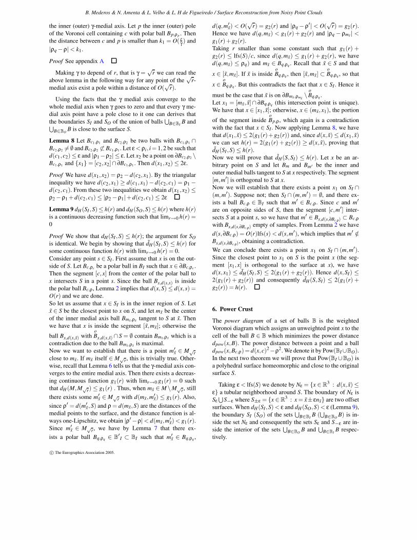
Figure 3: Bunny and hip-bone models. The vertices of the hip-bone model were randomly perturbed using Gaussian noise,while noisy points were added to the vertex set of the bunny model to increase the density. The bumpy but topologically correctoutputs shown here were produced by applying our modified power crust algorithm to the noisy point clouds.

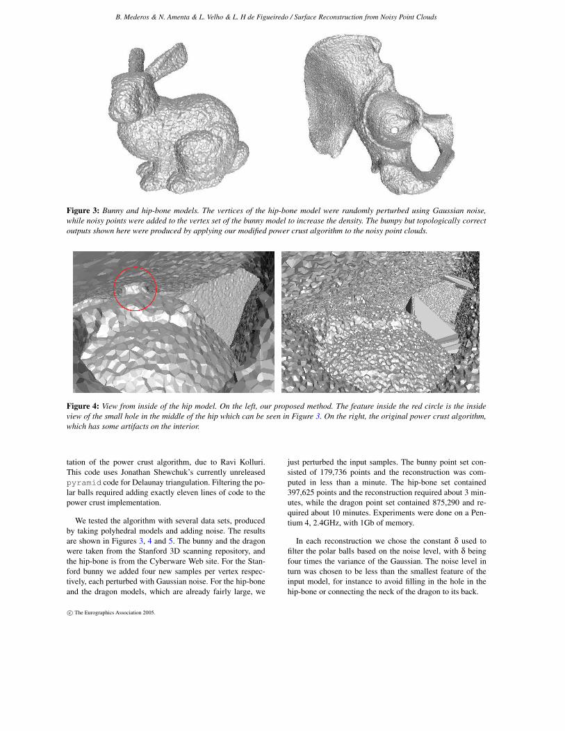
Figure 4: View from inside of the hip model. On the left, our proposed method. The feature inside the red circle is the insideview of the small hole in the middle of the hip which can be seen in Figure 3. On the right, the original power crust algorithm,which has some artifacts on the interior.

tation of the power crust algorithm, due to Ravi Kolluri.This code uses Jonathan Shewchuk’s currently unreleasedpyramid code for Delaunay triangulation. Filtering the po-lar balls required adding exactly eleven lines of code to thepower crust implementation.

We tested the algorithm with several data sets, producedby taking polyhedral models and adding noise. The resultsare shown in Figures 3, 4 and 5. The bunny and the dragonwere taken from the Stanford 3D scanning repository, andthe hip-bone is from the Cyberware Web site. For the Stan-ford bunny we added four new samples per vertex respec-tively, each perturbed with Gaussian noise. For the hip-boneand the dragon models, which are already fairly large, we

just perturbed the input samples. The bunny point set con-sisted of 179,736 points and the reconstruction was com-puted in less than a minute. The hip-bone set contained397,625 points and the reconstruction required about 3 min-utes, while the dragon point set contained 875,290 and re-quired about 10 minutes. Experiments were done on a Pen-tium 4, 2.4GHz, with 1Gb of memory.

In each reconstruction we chose the constant δ used tofilter the polar balls based on the noise level, with δ beingfour times the variance of the Gaussian. The noise level inturn was chosen to be less than the smallest feature of theinput model, for instance to avoid filling in the hole in thehip-bone or connecting the neck of the dragon to its back.



Figure 5: Reconstruction of the dragon model perturbed with Gaussian noise. The perturbed point cloud is shown on the left.

References

[AB99] AMENTA N., BERN M.: Surface reconstructionby voronoi filtering. Disc. Comput. Geom 22, 11 (Sept.1999), 481–502. 1, 5

[ABK98] AMENTA N., BERN M., KAMVYSSELIS M.: Anew voronoi-based surface reconstruction algorithm. InProceedings of SIGGRAPH (1998), pp. 415–421. 1

[ACDL02] AMENTA N., CHOI S., DEY T. K., LEEKHA

N.: A simple algorithm for homeomorphic surface recon-struction. Internat J. Comput. Geom & Applications 12(2002), 125–141. 1

[ACK] AMENTA N., CHOI S., KOLLURI R.: The powercrust. In Proceedings of 6th ACM Symposium on SolidModeling. 1

[ACK01] AMENTA N., CHOI S., KOLLURI R.: Thepower crust, union of balls and medial axis transform.Comput. Geom: Theory & Applications 22 (2001), 127–153. 1, 2, 3, 4, 6, 8, 12

[APR99] AMENTA N., PETERS T. J., RUSSELL. A.:Computational topology: Ambient isotopic approxima-tion of 2-manifolds. Comput. Geom: Theory & Applica-tions 22 (1999), C481–C504. 3

[BC00] BOISSONNAT J. D., CAZALS F.: Smooth sur-face reconstruction via natural neighbor interpolation ofdistance function. Proc. 16th. Annu. Sympos. Comput.Graphics 19 (2000), 223–232. 1

[BMR∗99] BERNARDINI F., MITTLEMAN J., RUSHMEIR

H., SILVA C., TAUBIN G.: The ball-pivoting algorithmfor surface reconstruction. IEEE Transactions on Visionand Computer Graphics 5, 4 (1999). 1

[CBC∗01] CARR J. C., BEATSON R. K., CHERRIE J. B.,MITCHELL T. J., FRIGHT W. R., MCCALLUM B. C.,EVANS T. R.: Reconstruction and representation of 3dobjects with radial basis functions. In Proceedings of SIG-GRAPH (2001), pp. 67–76. 1

[CFG∗03] CHEN W. S., FUNKE F., GOLIN M., KUMAR

P., POON H. S., RAMOS E.: Curve reconstruction fromnoisy samples. Proc. 19th Annu. Sympos. Comput. Geom.4, 11 (Sept. 2003), 302–311. 2

[CL96] CURLESS B., LEVOY M.: A volumetric methodfor building complex models from range images. In Pro-ceedings of SIGGRAPH (1996), pp. 303–312. 1

[CLar] CHAZAL F., LIEUTIER A.: The λ-medial axis.Graphical Models (to appear). 2

[DG04] DEY T. K., GOSWAMI S.: Provable surface re-construction from noisy samples . Discrete and Compu-tational Geometry 29, 3 (Sept. 2004), 15–30. 1, 3

[HDD∗92] HOPPE H., DEROSE T., DUCHAMP T., MC-DONALD J., STUETZLE W.: Surface reconstructionfrom unorganized points. In Proceedings of SIGGRAPH(1992), pp. 71–78. 1

[Kol05] KOLLURI R.: Provably good moving leastsquares. In Proceedings of ACM Symposium on DiscreteAlgorithms (2005). 2

[Lev03] LEVIN D.: Mesh-independent surface interpola-tion. In Geometric Modeling for Scientific Visualization,Brunnett G., Hamann B., Mueller K.„ Linsen L., (Eds.).Springer-Verlag, 2003. 2

[Lie04] LIEUTIER. A.: Any open bounded subset of r

has the same homotopy type as its medial axis. Journal



x

x

x y

h

y

y 1

2

1

2

ß

Figure 6: Given two points y1,y2 ∈ C(y) there exist twopoints x1,x2 ∈C(x) such that y1 ∈ B(x1,ε) and y2 ∈ B(x2,ε)

of Computer-Aided Design, 2004, in Press 29, 3 (Sept.2004), 12–16. 11

[LPC∗00] LEVOY M., PULLI K., CURLESS B.,RUSINKIEWICZ S., KOLLER D., PEREIRA L., GINZTON

M., ANDERSON S., DAVIS J., GINSBERG J., SHADE J.,FULK D.: The digital michelangelo project: 3D scanningof large statues. In Proceedings of SIGGRAH (2000),pp. 131–144. 1

Appendix A: γ Medial axis and medial axis approximation

Now we will presents some technical lemmas and defini-tions needed to prove rigorously that the γ-medial axis Mγconverges to the medial axis M. We use the following setfunction [Lie04] C from R3 onto the subsets of S which as-signs to x ∈ R3 the set C(x) = ∂Bx,d(x,S) ∩ S. (That is, C(x)is the set of points of S nearest to x.) The restriction of thisfunction C to the medial axis M is an upper semicontinuousfunction in the following sense.

Lemma 11 ([Lie04]) Given x ∈ M and ε > 0, there existsδ > 0 such that if d(x,y) ≤ δ, then C(y) ⊂C(x)+ B0,ε

Here C(x) + B0,ε represents the Minkowski sum. Basedon the definition of the function C we construct the functionα(m) = supx,y∈C(m) ∠( ~mx, ~my). Consequently Mγ = x ∈M : α(x) ≥ γ.

From Lemma 11 we have that the function α is an uppersemicontinuous function.

Lemma 12 Given ε > 0, there exists δ > 0 such that ifd(x,y) ≤ δ, then α(y) ≤ α(x)+ ε.

Proof let x1 and x2 be two points inside C(x) such thatsupp,q∈C(x) ∠(~xp, ~xq) = ∠( ~xx1, ~xx2), this two points exist be-cause C(x) is a compact set and the triangle x1xx2 is isosce-les. Let h be the projection of x onto the segment x1x2. Tak-

ing y1,y2 ∈ C(y) the maximum value of ∠( ~yy1, ~yy2) is ver-ified when the isosceles triangle y1yy2 is in the same planeof triangle x1xx2. One can see that ∠( ~yy1, ~yy2) is maximumwhen y is on the intersection of the segment xh with theboundary of the ball B(x,δ) and the points y1 and y2 areon the boundaries of the balls B(xi,ε) such that yyi are or-thogonal to xiyi for i = 1,2, see figure 6. From this one de-duces that ∠( ~yx1, ~yx2)≤∠( ~xx1, ~xx2)+2∠xx1y. Taking δ≤ εone obtain that cos(∠xx1y) ≥ d(x,x1)−d(x,y)

d(x,x1)≥ 1 − ε

lfs(S)≥

1 − O(ε), consequently ∠xx1y = O(ε) and ∠( ~yx1, ~yx2) ≤∠( ~xx1, ~xx2)+ O(ε).From this we have ∠( ~yy1, ~yy2)≤ ∠( ~yx1, ~yx2)+2∠( ~yy1, ~yx1)

where ∠( ~yy1, ~yx1) = arccos(√

d(y,x1)2−ε2

d(y,x1)) ≤

arccos(√

1− ( εlfs(S)−ε )2) = O(ε), therefore we obtain

α(y) ≤ α(x)+ ε1 with ε1 = O(ε).

As a consequence of the upper semicontinuity of the func-tion α we have that the set Mγ is a closed set, so it is a com-pact set due to Mγ ⊂ M and M is a compact set. The nextlemma plays an important role in the proof of Lemma 9

Lemma 13 Given any decreasing continuous function f :R → R such that limr→0 f (r) = 0 then g(r) = dH (M,M f (r))is a decreasing function and limr→0 g(r) = 0 = g(0).

Proof Let rkk=1,2,3,... a decreasing sequence of real num-ber converging to zero, then we have

M f (r1) ⊂ M f (r2) ⊂ M f (r3) ⊂ ·· · ⊂ M

Moreover, when j > i we have r j < ri and consequentlyM f (ri) ⊂ M f (r j) ⊂ M then we have g(ri) = dH (M f (ri),M) >g(r j) = dH(M f (r j),M). Because M is compact with M f(rk) ⊂M a sequence of compact subsets of M which M f (rk) ⊂M f (rk+1) for k = 1,2... we can use a know result state that ainclusion chain of compact set converge to its union in Haus-dorff distance. So the sequence M f (rk)k=1,2,... converge inthe Hausdorff metric to

S

k≥1 M f (rk) an therefore convergealso to its closure

S

k≥1 M f (rk) which is equal to M = M f (0)

by definition.As a consequence of this, the function g(r) = dH (M,M f (r))is a decreasing function which is continuous at zerolimr→0 g(r) = 0 = dH(M,M f (0)) and its easy to see thatthere exists a continuous function h(r) such that h(r) ≥ g(r)and limr→0 h(r) = 0

We also have that for any point in the in the γ-medial axisthere exist a point within a distance of O(r/γ).

Lemma 14 Let Bc,ρ be a medial ball such that c belongs tothe inner (outer) γ-medial axis. Let p the inner (outer) poleof the Voronoi cell containing c with polar ball Bp,ρp . Thenthe distance between c and p is smaller than k1 = O( r

γ ) and|ρq −ρ| < k1.

Proof Let h be the closest sample to c, then p is the inner(outer) pole of h. Let u1,u2 be two points in ∂Bc,ρ ∩ S suchthat ∠u1cu2 ≥ γ, let γ be the maximum of angles ∠hcu1 and∠hcu2, let u ∈ u1,u2 be the one realizing γ.



Let l be the ray with origin at c and containing the segment[h,c], this ray intersects ∂Bc,ρ at the point x. If h ∈ Bc,ρ, thenusing that h /∈Bc,ρ then d(h,x)≤ d(h, h) = k1 ·r · lfs(h). Let ube the closest sample to u. Then, when h /∈ Bc,ρ we have thatρ + d(u,u) ≥ d(c,u) ≥ d(c,h) = ρ + d(x,h), consequentlyd(x,h)≤ d(u,u)≤ k1 ·r · lfs(u). Hence in either case h /∈ Bc,ρor h ∈ Bc,ρ we have that d(x,h) ≤ k1 · r ·ρ.Now we will bound the angle ∠phu≤∠phc+∠chu+∠uhu.By lemma 4 we get ∠phc = O(

√r). When h /∈ Bc,ρ we have

that ∠chu ≤ ∠cxu ≤ π2 − γ

2 . When h ∈ Bc,ρ we have that∠chu = ∠cxu+∠xuh, the angle ∠cxu = π

2 −γ2 and the angle

∠xuh is smaller than arcsin(d(h,x)d(x,u) ) = arcsin( k1·r·ρ

2ρ sin( γ2 )

) using

that sin(y) ≥ 56 y for y < 1, we obtain arcsin(

d(h,x)d(x,u)

) = O( rγ ).

Hence we have ∠chu ≤ π2 − γ

2 + O( rγ ).

Let us bound the angle ∠uhu. Let us denote by H the hy-potenuse of the triangle uhu, we have that H ≥ d(h, u) ≥d(x, u)−d(x,h) ≥ 2ρ sin( γ

2 )− k1 · r ·ρ > 0. Hence ∠uhu =

arcsin( d(u,u)H ) = arcsin( k1·r·ρ

2ρ sin( γ2 )−k1·r·ρ

) = O( rγ )

From these computations we conclude that ∠phu ≤ π2 −

γ2 +

O(√

r)+ O( rγ ).

Let T be the hyperplane orthogonal to the segment hu andpassing through its midpoint. Since d(p,h) ≤ d(p,u) wehave that p is inside the half space of T containing h andthis implies

d(p,h) ≤ d(h,u)/2sin( π

2 −∠phu)(13)

Using that sin( γ2 −O(

√r)−O( r

γ )) ≤ sin( γ2 )cos(O(

√r) +

O( rγ )) and that d(h,u) ≤ d(h,x) + d(x, u) + d(u,u) ≤

2ρ sin(γ)2 )+ O(r)ρ we deduce from 13 that

d(p,h) ≤ ρcos(O( r

γ )+ O(√

r))+

O( rγ )ρ

cos(O( rγ )+ O(

√r))

Denote by l = ρcos(O( r

γ )+O(√

r)) +O( r

γ )ρcos(O( r

γ )+O(√

r)) . Hence

d(c, p) ≤ d(p,h) − d(c,h) ≤ l − ρ + O(r)ρ = O( rγ )ρ and

|ρp −ρ| = |d(p,h)−d(c,x)| ≤ |l−ρ| = O( rγ ).

Observe that this lemma is valid for γ = f (r) with f (r) acontinuous function such that limr→0 r f (r) = 0.

Appendix B: Labeling Algorithm

Once we have determined the set P′ of polar balls to be re-tained in the noisy version of the power crust algorithm, andcomputed their power diagram, the next step of the algorithmis to label each of the balls in P′ as an outer or inner ball, thusdetermining the sets BI and BO. We use exactly the same la-beling algorithm as in the original power crust implementa-tion [ACK01], but we explain it here for completeness. Thenwe prove a couple of lemmas which guarantee that the label-ing algorithm is correct. These proofs a similar to analogous

proofs in the noise-free case, but again we include them forcompleteness.

For each sample in the special set Z of vertices of thebounding box, its polar ball is inserted in a queue and la-beled as outer. Then we iteratively propagate the labeling.While the queue is not empty, we remove a ball Bp from thequeue. We examine each of the balls Bq whose cells neigh-bor that of Bp in the power diagram of P′. If the intersectionbetween Bp and Bq is at a angle bigger than π/4, we assignto Bp the same label as Bq. Also we assign the opposite labelto the ball of the other pole of p, if there is one. This processis repeated until there is not a new ball that can be classi-fied as outer or inner. Once we have finished the labeling wedetermine the faces in Pow(P′) separating inner balls fromouter ones.

Lemma 15 The angle of intersection between a polar ballBc1,ρ1 ∈BI and a polar ball Bc2,ρ2 ∈BO with Bc2,ρ2 ∩Bc1,ρ1 6=∅ is O(r).

Proof We have that the center c1 and c2 of Bc1,ρ1 and Bc2,ρ2

are in different sides of S, thus the segment [c1,c2] intersectsthe surface at a point x ∈ S. Let bi = [c1,c2]∩∂Bci,ρi withi = 1,2.The ball Bx,d(x,bi) is inside Bci,ρi which is empty of sam-ples. Then by lemma 2 we obtain that d(x,bi) = O(r)lfs(x).Hence d(b1,b2) ≤ d(x,b1) + d(x,b2) ≤ O(r)lfs(x), conse-quently d(b1,b2) ≤ O(r)maxx∈S lfs(x) = O(r)∆1.Let Π a plane containing the intersection circle between theballs Bc1,ρ1 and Bc2,ρ2 and z = Π∩ [c1,c2]. Let us boundthe distance ci to z we have that d(ci, z) ≥ ρi − d(b1,b2) ≥ρi −O(r)∆1. Since that ρi ≥ lfs(S)/c, then for small enoughr we have:

cos(αi)=d(ci, z)

ρi≥ ρi −O(r)∆1

ρi≥ 1−O(r)

c∆1lfs(S)

= 1−O(r)

Hence we have that αi = O(r) for i = 1,2 and the angle be-tween the two balls is α1 + α2 = O(r)

Lemma 16 Let ε be smaller than lfs(S). Given a point u anda ball Bc,ρ ∈ BI (Bc,ρ ∈ BO) such that d(u,∂Bc,ρ) ≤ O(ε)and u ∈ Nε, then the angle between the vector ~cu and theoutward (inward) normal~nu is O(

√ε).

Proof Let Bm,ρm be the outer medial axis ball tangent to Sat u and let Bc,ρ ∈ BI be a ball such that d(u,∂Bc,ρ) = O(ε).Let Nε be a tubular neighborhood of S. It is easy to see thatthe ball Bm,ρm−ε is inside the outer solid which is delimitedby Sε and Ω, therefore Bc,ρ ∩Bm,ρm−ε = ∅.The points c, m and u form a triangle and the point t isthe projection of u onto the segment cm. Our aim is tofind an upper bound for angle between the vectors ~cu and~nu which is θ = ∠(m,c,u) + ∠(u,m,u) see figure 7. We

have the following identities ∠(c,m,u) = arcsin(

d(u,t)d(u,m)

)

and ∠(m,c,u) = arcsin(

d(u,t)d(u,c)

)

.



S

Sε

m

umtm

uctc

u

Bc,ρ

Bm,ρm−ε

c

t

θ

Figure 7: The angle θ between the vector ~cu and the normal~nu at u

.

There are three possibilities: t ∈ Bm,ρm−ε, t ∈ Bc,ρ andt /∈ Bm,ρm−ε

S

Bc,ρ. When t ∈ Bm,ρm−ε (t ∈ Bc,ρ) us-ing the equations d(u, t) =

√

d(u,m)2 −d(t,m)2 andd(u, t) =

√

d(u,c)2 −d(t,c)2 one deduce that d(u, t) ≤√

(ρ + d(u,∂Bc,ρ))2 −ρ2 = O(√

ε) when t ∈ Bm,ρm−εand in the other case t ∈ Bc,ρ we get d(u, t) ≤√

(ρm + d(u,∂Bm,ρm−ε))2 −ρ2m = O(

√ε). From this two

bounds of the distance d(u, t) we obtain that

∠(c,m,u) ≤ arcsin(

d(u, t)

ρm −√

ρ2m −d(u, t)2

)

= O(√

ε)

∠(m,c,u) ≤ arcsin(

d(u, t)

ρ−√

ρ2 −d(u, t)2

)

= O(√

ε)

Now consider t /∈ Bm,ρm−εS

Bc,ρ. Let tmum with um ∈∂Bm,ρm be a segment parallel to ut and intersecting the seg-ments cm also let tcuc be parallel segment to tu with uc ∈∂Bc,ρ and tc ∈ uc. From this we get that

∠(c,m,u) = arcsin(

d(um, tm)

ρm

)

(14)

∠(m,c,u) = arcsin(

d(uc, tc)ρ

)

(15)

Due to d(um, tm) ≤√

(ρm −d(u,∂Bm,ρm−ε))2 −ρm2 =

O(√

ε) and d(uc, tc) ≤√

(ρ−d(u,∂Bc,ρ))2 −ρ2 = O(√

ε)we obtain that ∠(c,m,u) = O(

√ε) and ∠(m,c,u) = O(

√ε)

Corollary 1 The angle of intersection between two ballsBc1,ρ1 ∈ BI and Bc2,ρ2 ∈ BI such that Bc1,ρ1 ∩Bc2,ρ2 ∩Nε 6= ∅,is π−O(

√ε).

Proof Take x ∈ Nε ∩ Bc1,ρ1 ∩ Bc2,ρ2 . We have thatd(x,∂Bci,ρi) = 0 for i = 1,2.

Therefore, applying the lemma 16 we have the angle be-tween the surface normal ~nx and the vector ~cix, is O(

√ε)

for i = 1,2, consequently the angle between the vectors ~c1xand ~c2x is O(

√ε) and the angle between the tangent planes

at x is π−O(√

ε).


Surface Reconstruction from Noisy Point Cloudsamenta/pubs/boris.pdf · B. Mederos & N. Amenta & L....

Documents

Transcript of Surface Reconstruction from Noisy Point Cloudsamenta/pubs/boris.pdf · B. Mederos & N. Amenta & L....