Clemson UniversityTigerPrints

All Theses Theses

5-2012

Surface Characterization of Nephila clavipesDragline SilkBenoit FaugasClemson University, ben.faug@gmail.com

Follow this and additional works at: https://tigerprints.clemson.edu/all_theses

Part of the Materials Science and Engineering Commons

This Thesis is brought to you for free and open access by the Theses at TigerPrints. It has been accepted for inclusion in All Theses by an authorizedadministrator of TigerPrints. For more information, please contact kokeefe@clemson.edu.

Recommended CitationFaugas, Benoit, "Surface Characterization of Nephila clavipes Dragline Silk" (2012). All Theses. 1370.https://tigerprints.clemson.edu/all_theses/1370

SURFACE CHARACTERIZATION OF NEPHILA

CLAVIPES DRAGLINE SILK

A Thesis

Presented to

the Graduate School of

Clemson University

In Partial Fulfillment

of the Requirements for the Degree

Masters of Science

Materials Science and Engineering

by

Benoit Faugas

May 2012

Accepted by:

Prof. M. Ellison, Committee chair (Clemson University)

Prof. M. Kennedy (Clemson University)

Prof. D. Dean (Clemson University)

Prof. E. Fargin (University of Bordeaux 1)

Prof. J-L. Bobet (University of Bordeaux 1)

ii

ABSTRACT

To design synthetic fibers for extreme applications, many research groups are

trying to identify how the structure of natural fibers (such as spider silk) leads to

desirable properties such as high tensile strength.

Spider silk is a biological fiber having mechanical properties that exceed those of

the best man made fibers in terms of high tensile strength and large extensibility, this

combination providing the silk with a large work of rupture. While the bulk structure,

composition and properties have been intensively studied elsewhere, this study

focuses on elucidating the Nephila clavipes spider dragline silk surface structure and

composition, as well as examining the possibility of a pattern to the arrangement of

the amino acids on the surface. These spiders are traditionally studied since they are

orb weaving spiders with relatively high silk toughness values. While these spiders

fabricate several types of silk, all with different biological uses, this study focuses

only on dragline silk.

The silk surface morphology was observed initially using contact mode atomic

force microscopy in 0.01 M phosphate buffered saline (PBS) solution. In general, the

roughness of dragline silk, which has a nominal diameter of five micrometers, was

found between 20 nm and 100 nm. We studied the roughness as a function of the

collection speed and of age of the silk (time since collection). It was found that

surface roughness is independent of collection speed: values are included in the same

range of values (40 nm to 60 nm) and no trend is demonstrated. Roughness study as a

function of time since collection also showed that there is no change in roughness as

the fiber ages. This demonstrates the surface stability of the dragline silk over time in

terms of roughness. There were surface features that may have been cracking in a

iii

worm-like fashion which may have been formed by stretching during sample

preparation.

To determine the arrangement of amino acids along the dragline silk,

functionalized gold nanoparticles were used to “mark” the charged amino acid

locations. The gold nanoparticles functionalized with COOH groups (respectively,

NH2 groups) are used to find positively charged (respectively, negatively charged)

amino acids. The density of negatively charged amino acids (glutamic acid, aspartic

acid) is higher than that of the positively charged ones (lysine, asparagine, and

histidine). This correlates with the relative amounts of amino acids found by amino

acid analysis by other researchers [2.1, 2.2, 2.3]. A pattern might have been found in

the arrangement of negatively charged amino acids, in that they might be spaced with

a certain frequency at some locations, but additional work is needed to confirm this.

On the other hand, positively charged amino acids were randomly arranged on the

surface.

iv

ACKNOWLEDGEMENTS

I would like to thank Prof. Ellison for accepting me in his group and giving me this

project to work on. I also thank him for teaching me the way to think, do research, and

for the valuable discussions we had. Thank you for everything!

I show my gratitude to Prof. Dean and Prof. Kennedy. Thank you for taking your

time to serve in my committee and for providing me support and guidance, with

patience.

Big thanks to Prof. Richardson, Prof. Fargin and Prof. Bobet for accepting me in

the MILMI program and giving me the opportunity of doing the second year of my

master in Clemson.

I also want to thank Prof. Dean for teaching me AFM, Mr. Donald Mulwee for

teaching me SEM, Ms. Janci Despain for her previous job done on spiders, Mr. Taras

Andrukh for setting up the silk collection instrumentation and Mr. James Chow for

helping me with functionalizing gold nanoparticles.

Thanks to the MS&E staff and faculty for providing me help when needed with

administration: Dr. Lickfield, Dr. Luzinov, Ms. Kathy Bolton, Mr. Robert Bowen,

Ms. Tonya Bledsoe, and Ms. Shelby Sheriff.

And thanks to the awesome graduate students that made my year wonderful!

The MILMI master is funded by the Atlantis program which supports the

cooperation between EU and US higher education institutions. Funding support is

both provided by the Department of Education of the United States Government under

the contract #P116J080033 University of Central Florida and the European

Commission under the contract #2008-1750/001-001 CPT-USTRAN Université

Bordeaux 1.

v

TABLE OF CONTENTS

Page

TITLE PAGE ................................................................................................................. i

ABSTRACT .................................................................................................................. ii

ACKNOWLEDGEMENTS ......................................................................................... iv

LIST OF FIGURES ................................................................................................... viii

LIST OF TABLES .......................................................................................................xv

CHAPTER

1. Introduction to spider silk ........................................................................................1

1.1. Background on N. clavipes spider .....................................................................2

1.1.1. Spiders and spider silk .............................................................................2

1.1.2. Structure of spider dragline silk ...............................................................4

1.1.3. Chemical composition of spider dragline silk .........................................5

1.1.4. Mechanical properties ..............................................................................7

1.2. Surface analysis .................................................................................................8

2. Characterization methods for chemical, mechanical and

structural properties ......................................................................................10

2.1. Composition and structure ...............................................................................10

2.1.1. Amino acid analysis ...............................................................................10

2.1.2. X-ray diffraction ....................................................................................11

2.2. Surface .............................................................................................................14

2.2.1. Atomic force Microscopy ......................................................................14

2.2.1.1. AFM instrument description .........................................................14

2.2.1.2. AFM operation ..............................................................................16

vi

2.2.2. Electron Microscopy ..............................................................................19

2.2.3. Optical Microscopy................................................................................23

2.3. Physical properties ...........................................................................................24

2.3.1. Mechanical property tests ......................................................................24

2.3.2. Thermal analysis ....................................................................................26

3. Investigation of spider dragline silk surface morphology ......................................29

3.1. Materials and Methods .....................................................................................29

3.1.1. Spider silk ..............................................................................................29

3.1.1.1. Collection .................................................................................29

3.1.1.2. Sample preparation ..................................................................31

3.1.2. Atomic Force Microscope .....................................................................31

3.2. Experimental design .........................................................................................32

3.2.1. Roughness experiments .........................................................................32

3.2.2. Verifying that AFM scanning of surface is a

nondestructive technique ...............................................................34

3.2.3. Average roughness repeatability experiment ........................................34

4. Characterization of amino acids on the surface of spider

dragline silk ......................................................................................................36

4.1. Materials and Methods .....................................................................................36

4.1.1. Spider silk ..............................................................................................36

4.1.2. Labeling of carboxyl and amine groups with

gold nanoparticles ..........................................................................37

4.1.3. Sample preparation ................................................................................39

4.1.4. Scanning electron microscope ...............................................................39

vii

4.2. Experimental design .........................................................................................40

5. Results ....................................................................................................................43

5.1. Roughness ........................................................................................................43

5.2. Verifying that AFM scanning of surface is a

nondestructive technique ...........................................................................44

5.3. Average roughness repeatability ......................................................................47

5.4. Roughness as a function of reeling speed ........................................................48

5.5. Amino acids characterization on spider dragline silk surface ..........................50

6. Discussion ..............................................................................................................53

7. Conclusions ............................................................................................................60

APPENDICES .............................................................................................................62

A. AFM set up ......................................................................................................63

B. Amino acids structure ......................................................................................67

C. Sample size determination ...............................................................................69

D. Additional images ............................................................................................70

REFERENCES ............................................................................................................72

viii

LIST OF FIGURES

Chapter 1

Figure Page

1.1 Picture of a N. clavipes female spider ................................................................2

1.2 Picture of the spinnerets of a N. clavipes spider used to

produce dragline silk (Photo credit: Janci Despain) ......................................4

1.3 (Left) Microscopic representation of dragline silk fiber;

(Right) Large crystalline domain (black arrow) and

small crystalline domain (red arrow) connected together

via an amorphous domain ..............................................................................5

1.4 Amino acid sequence of MaSp1 showing the alanine

block “AAAAAA” and the glycine-rich region ............................................6

1.5 Part of the polypeptide chain made of alanine amino

acids linked together via hydrogen bonds, forming

antiparallel -sheet nanocrystals ...................................................................7

ix

Chapter 2

Figure Page

2.1 SAXS operation. A well-collimated X-ray beam is focused

on the specimen and the scattered beam intensity is recorded

as a function of angle between the incoming beam and

the scattered beam .......................................................................................12

2.2 Image of an Atomic Force Microscope: (1) Microscope;

(2) Head part; (3) Stage; (4) Anti-vibration table ........................................15

2.3 Scheme of AFM measurement principle. The tip approaches

the surface and interacts with it, making the cantilever to

deflect. The reflected angle of the laser on the cantilever

will then change and be detected on the photodiode,

providing the topography of the surface ......................................................17

2.4 A schematic representation of the Contact mode ............................................18

2.5 SEM operation. Electron beam is produced by the electron

gun and is guided towards the sample by passing

through an anode and magnetic lenses. Scanning coils

rasters the beam across the surface and the SE and BSE

are collected by detectors ............................................................................20

2.6 TEM operation. An electron beam is guided up to the

specimen where electrons go through it. The electrons that

cross the specimen are then used to produce the image ..............................22

2.7 CLSM operation. A laser light is focused on the sample by

an objective lens. The emitted light is recollected by the lens

and guided to the detector by a beam splitter. The detector

aperture selects the light coming from the focal plane only,

removing the light coming from above or below the focal

plane (dashed lines) .....................................................................................24

2.8 Instron Tester used for studying tensile properties ..........................................25

x

Chapter 3

Figure Page

3.1 (Left) Picture of a take-up reel with (1) the spool and

(2) the reeling motor. (Right) Picture of a N. clavipes spider

stapled onto a Styrofoam block in order to extract silk

from her spinnerets (Photo credit: Janci Despain) ......................................30

3.2 Relevant anatomy of the spinnerets. (1) Anterior lateral

spinneret that houses one major ampullate spigot on

its underside. (2) Major ampullate spigot that produces

dragline silk. One major ampullate spigot is located on

the underside of each anterior lateral spinneret.

(3) Dragline silks produced by each major ampullate

spigot. (Photo Credit: Janci Despain) ..........................................................30

3.3 Two spider silk fibers mounted on a microscope slide.

The fibers are difficult to see on this picture since they

are very thin. The dots of glue indicate the path of the fibers .....................31

3.4 Schematic representation of the experiment.

The spider silk fiber is represented with the cylindrical

shape and the squares represent one image taken on one spot.

Each column (A, B, C…) corresponds of a series of 3 images

taken on the same spot .................................................................................35

xi

Chapter 4

Figure Page

4.1 Reaction used for attaching functionalized gold

nanoparticles to the specific charged amino acids on the

spider dragline silk surface ..........................................................................38

4.2 (Left) Formula of 11-Amino-1-undecanethiol.

(Right) Formula of 11-mercaptoundecanoic acid .......................................38

4.3 Steps preparation for attaching gold nanoparticles

functionalized with COOH groups to the negatively

charged amino acids. A switch between

11-Amino-1-undecanethiol and 11-mercaptoundecanoic acid

needs to be done to attach gold nanoparticles to the

positively charged amino acids ...................................................................39

4.4 Example of glycoprotein with a carbohydrate moiety

linked to a serine amino acid via O-linkage ................................................42

xii

Chapter 5

Figure Page

5.1 Height and deflection image of N. clavipes spider

dragline silk reeled up at 2.16 mm.s-1

analyzed on

08/16/2011 in air. The size of the image is 4 µm x 2 µm.

The surface roughness is 63.1 nm ...............................................................43

5.2 Height and deflection image of N. clavipes spider

dragline silk reeled up at 0.72 mm.s-1

analyzed on

08/19/2011 in fluid. The size of the image is 3 µm x 3 µm.

The surface roughness is 63.5 nm ...............................................................44

5.3 Height images of spider silk surface conducted in fluid

with a scan area of 1 µm x 1 µm. The image on the left is

the image of the first scan. The image on the right is the

image of the fifth scan as we scan the same spot ........................................45

5.4 Height images of spider silk surface conducted in fluid

with a scan area of 2 µm x 2 µm. The image on the left is

the image of the first scan. The image on the right is the

image of the fifth scan as we scan the same spot ........................................45

5.5 Roughness changes with scanning a same spot with a scan

area of 1 µm x 1 µm (blue diamonds) and with scanning

the same area but with a scan size of 2 µm x 2 µm

(red squares) ................................................................................................46

5.6 Roughness changes with scanning the same spot eleven

times in a row ..............................................................................................47

5.7 Collection speed effect on surface roughness. The blue

diamonds represent a five years old spider silk whereas

red diamonds represent fresh spider silk .....................................................49

5.8 Backscatter SEM images of spider dragline silk with

COOH functionalized gold nanoparticles bound to lysine,

arginine and histidine residues. (Left) Fiber glued at its end

on a microscope slide. (Right) Fiber stuck on double carbon

tape substrate ...............................................................................................50

xiii

5.9 Backscatter SEM images of spider dragline silk with NH2

functionalized gold nanoparticles bound to glutamic

acid and aspartic acid residues. (Left) Fiber fixed on

double coated carbon tape and stretched. (Right) Fiber glued

at its end on a microscope slide ...................................................................51

5.10 Backscatter SEM images of a spider dragline silk with NH2

functionalized gold nanoparticles bound to glutamic

acid and aspartic acid residues coated with a thin layer of Pt .....................51

5.11 Backscatter SEM images of a bundle of spider dragline

silks fixed on doublecarbon tape substrate with COOH

functionalized gold nanoparticles bound to lysine,

arginine and histidine residues ....................................................................52

5.12 Backscatter SEM images of a bundle of spider dragline

silks fixed on doublecarbon tape substrate with NH2

functionalized gold nanoparticles bound to glutamic acid

and aspartic acid residues ............................................................................52

xiv

Chapter 6

Figure Page

6.1 Scheme explaining how gold nanoparticles do not appear.

(a) Side look of the spider dragline silk with functionalized

gold nanoparticles attached to it. (b) Top view of this

same spider dragline silk as if using SEM, showing that

gold nanoparticles at the bottom of the

fiber in (a) are missing .................................................................................58

xv

LIST OF TABLES

Table Page

1.1 Comparison of mechanical properties between N. clavipes

dragline silk fiber and Kevlar® 49 fiber. The very high

elasticity of the spider dragline silk combined with a

high tensile strength makes it tougher than the

Kevlar® 49 fiber.............................................................................................8

2.1 Table of results on the amino acid composition of

N. clavipes spider silk found in literature [2.1, 2.2, 2.3] .............................11

3.1 Three different orders of flattening and their effect on the image ...................33

5.1 Average roughness data for the experiment shown in

Figure 3.4. The values of the rows I, II and III are

used to determine the repeatability ..............................................................48

5.2 Data for the surface roughness of N. clavipes spider

silk obtained for five different collection speeds ........................................49

1

CHAPTER ONE

INTRODUCTION TO SPIDER SILK

Biomimetics is the study of biological materials or systems to identify design

constructs that can lead to innovative synthetic material designs. Discoveries in the

field of biomimetics have been used to improve the efficiency of existing materials

based on natural design. Examples include reducing the drag on airplane wings (or

wind turbine blades) by mimicking the humpback whale flipper shape [1.1],

reproducing lotus leafs’ surface microstructure to get a self-cleaning surface

(application in paint with StoCoat Lotusan®) [1.2] or mimicking Gecko’s foot surface

to create strong adhesive [1.3]. In the field of fibers, having the opportunity to create a

strong fiber that can work and not degrade in different environments will be very

beneficial in many domains. Spider dragline silk is a strong fiber, and understanding

its structure-property relationships will enable developing a mimic of it. A fiber such

as spider silk will find its place in environments ranging from medical applications for

tissue engineering ligaments to military application for bulletproof vest for example.

Spider silk is a natural fiber, and in terms of its mechanical properties of high

tensile strength and large extensibility, the silk has a large work of rupture [1.4].

Hence, scientists have investigated silk structure, composition and properties in order

to produce a better design for mimicking such a fiber. Nonetheless, the surface

structure and composition of dragline silk from Nephila clavipes has not been the

topic of very much research. The research in this study is focused on the surface of

natural N. clavipes spider dragline silk. The morphology of the spider dragline silk

surface and its amino acids content will be investigated.

2

1.1. Background on N. clavipes spider

1.1.1. Spider and spider silk

These past few years, studies revealed the structure and chemical content of spider

silk. One of the spiders whose silk has great mechanical properties is the N. clavipes

spider, also known as “Golden orb-weavers” due to the yellowish color of its web, or

“Banana spider” due to the alternation of gold and black color on its legs (Figure 1.1).

Figure 1.1: Picture of a N. clavipes female spider.

This type of spider is mostly found from the South/Southeast part of the United

States (South Carolina, Florida) to Argentina where the weather is warm and humid,

especially during the summer and fall. They are easily recognizable with their large

body and gold bright colors, and also by the big orb webs they can build (up to one

meter in diameter). Their diet is essentially composed of flying insects such as

butterflies, moths or bees and they can eat insects half as big as their own body. Their

venom is harmless for humans; the bite will only give local pain with redness [1.5].

3

By looking at their webs, one may think that the web is only made of one type of

silk. But this is not the case, many different silks are found on their web, each of them

having their own function. Actually, we find the following 7 types of silk [1.6]:

Major Ampullate silk, used to build the frame of the web and which is also the

“safety line” for the spider allowing her to not fall and crash when she is

pushed off her web.

Minor Ampullate silk, used to strengthen the frame and gives this typical

spiral shape.

Flagelliform silk, used to catch the prey and gives this circle shape of the web.

Aggregate silk, which is used as a sticky coating on the flagelliform silk (so

that the prey sticks to the web).

Pyriform silk, used to attach the frame on substrates.

Aciniform silk, used to wrap the prey.

Cylindriform silk, use to build egg sack.

All these fibers are formed by a complex spinning process and chemical reactions

before coming out of the spinnerets of the spider (Figure 1.2).

In this study, the most interesting and most studied spider silk is the Major

Ampullate silk, which exhibits high mechanical properties. Here, we will review the

structure of the dragline silk of the N. clavipes spider from the microscopic to

nanoscopic scale level with its chemical composition, and some properties.

4

Figure 1.2: Picture of the spinnerets of a N. clavipes spider, used to produce dragline

silk (Photo credit: Janci Despain).

1.1.2. Structure of spider dragline silk

Spider dragline silk is a cylindrical thread about three microns to five microns in

diameter, which varies along the fiber [1.7]. It is composed of three layers (cited in

order from the outermost layer to the inner part of the fiber): an outer layer, a skin

layer and then the core. The outer layer is essentially made of lipids and/or

glycoproteins for protection against the environment [1.8]. The core is composed of

many thread-like structures (fibrils) which are about 100 to 150 nm in size and that

are lined up along the fiber axis [1.9]. Inside these fibrils, several crystallite domains

are attached together via a semi-amorphous domain [1.10] (Figure 1.3).

5

Figure 1.3: (Left) Microscopic representation of dragline silk fiber; (Right) Large

crystalline domain (black arrow) and small crystalline domain (red arrow) connected

together via an amorphous domain [1.6].

1.1.3. Chemical composition of spider dragline silk

As a biological fiber, spider silk is mainly composed of proteins [1.10]. Proteins

are polypeptides; that is, polymer chains comprised of amino acids that are linked

together by peptide bonds between carboxyl (COOH) and amino (NH2) groups. In

silk, these proteins are diblock copolymers, commonly called spidroins. Spider

dragline silk is produced by a specific gland called the major ampullate gland, and the

two main proteins that constitute the dragline silk are named major ampullate spidroin

1 (MaSp1) and major ampullate spidroin 2 (MaSp2).

MaSp1 is a protein consisting of 747 amino acids and is made of 25 motifs repeats.

In each motif repeats we have a polyalanine block (consisting only of alanine amino

acids linked together) followed by a glycine-rich region (Figure 1.4). In the case of

MaSp1, the glycine-rich region is mostly made of GGA and GGX motifs, with “A”

standing for the amino acid alanine, “G” for glycine and “X” being another amino

acid (glutamine/glutamic acid, tyrosine, serine, leucine). This glycine-rich part has

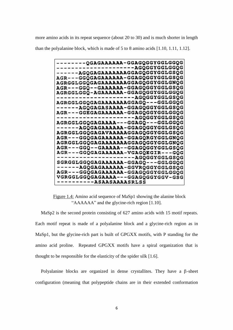
6

more amino acids in its repeat sequence (about 20 to 30) and is much shorter in length

than the polyalanine block, which is made of 5 to 8 amino acids [1.10, 1.11, 1.12].

Figure 1.4: Amino acid sequence of MaSp1 showing the alanine block

“AAAAAA” and the glycine-rich region [1.10].

MaSp2 is the second protein consisting of 627 amino acids with 15 motif repeats.

Each motif repeat is made of a polyalanine block and a glycine-rich region as in

MaSp1, but the glycine-rich part is built of GPGXX motifs, with P standing for the

amino acid proline. Repeated GPGXX motifs have a spiral organization that is

thought to be responsible for the elasticity of the spider silk [1.6].

Polyalanine blocks are organized in dense crystallites. They have a -sheet

configuration (meaning that polypeptide chains are in their extended conformation

7

and are linked to their neighbors by hydrogen bonds) and these -sheet nanocrystals

are antiparallel (Figure 1.5) [1.10, 1.13, 1.14]. The size of these nanocrystals is not

regular but is about 53 Å × 47 Å × 60 Å with a separation distance of 7 nm to 8 nm

between two of them [1.15]. These nanocrystals are thought to be responsible for the

enhancement in mechanical properties relative to the amorphous domain because they

form a stiff cross-link network (due to hydrogen bonds) [1.16]. The glycine-rich

region is found in the semi-amorphous matrix separating polyalanine blocks, having

31-helix type structures and beta-turns [1.17].

Figure 1.5: Part of the polypeptide chain made of alanine amino acids linked

together via hydrogen bonds, forming antiparallel -sheet nanocrystals.

1.1.4. Mechanical properties

Spider dragline silk from N. clavipes exhibits mechanical properties that

outperform the best man-made fibers such as Kevlar®. Tensile strength, Young’s

modulus and rupture elongation (elasticity) are summarized in Table 1.1 [1.4]. The

rupture elongation is on average 18 % but some silks presented a rupture elongation

8

above 30%. The combination of high tensile strength and elasticity is the key for

having a strong fiber.

Another property of spider dragline silk is its ability to shrink when wetted: this

effect is called “supercontraction”. When put in a humid environment (above 60 %

humidity) the spider silk shrinks in length up to 50 % [1.13] and also swells in

diameter [1.18]. Masp2 has been identified as the protein responsible for this effect,

and since MaSp2 has a high content of the amino acid proline, this component is at

the very origin of this effect [1.13, 1.19, 1.20, 1.21].

Table 1.1: Comparison of mechanical properties between N. clavipes dragline silk

fiber and Kevlar® 49 fiber. The very high elasticity of the spider dragline silk

combined with a high tensile strength makes it tougher than the Kevlar® 49 fiber

[1.22, 1.23].

Material Tensile

strength (GPa)

Young’s

modulus (GPa)

Rupture

elongation (%)

Toughness

(MJ/m3)

N. Clavipes

dragline silk

1 12.7 18 80

Kevlar® 49 2.9 105 2.5 50

1.2. Surface analysis

A surface can be smooth or rough and the surface features can exhibit different

shapes. Moreover, surfaces can be very different from the bulk, differing in chemical

composition, geometry and structure. At first sight, it can be thought that the

9

properties of a material are related to its internal structure; however, studying the

surface also has its importance. The knowledge of all the surface parameters listed

above will lead to a better understanding of the structure-property relationship.

Insights on the chemical composition, mechanical properties or behavior in different

environments can be obtained from surface analysis.

Spider silk fiber is considered as a semi-crystalline bio-copolymer and it is

important to know how the surface looks (not only on the microscopic level but also

on the nanoscopic level). Giving an insight of the spider silk surface will help

scientists to synthesize the fiber or modify it in order to enhance its properties.

10

CHAPTER TWO

CHARACTERIZATION METHODS FOR CHEMICAL, MECHANICAL AND

STRUCTURE PROPERTIES

Techniques of characterization that were originally developed for non-biological

materials such as atomic force microscopy or scanning electron microscopy have been

used for biological systems and have demonstrated their effectiveness. These

techniques need to be used with appropriate considerations and in proper conditions to

be effective. This chapter will summarize some characterization techniques used to

reveal properties of spider dragline silk.

2.1. Composition and structure

2.1.1. Amino acid analysis

Results from amino acid analysis performed by scientists [2.1, 2.2, 2.3] on N.

clavipes spider dragline silk are summed up in Table 2.1. From all these results, there

is a correlation for a high content of glycine (around 40 %) and alanine (around 25

%). Also, a non-negligible content of glutamine/glutamic acid (9 %), leucine (4 %),

tyrosine (3 %), serine (4 %), arginine (2 %), proline (1 %), aparagine (1.5 %), valine

(1 %) and lysine (1 %) is reported.

The amino acid content of five different spiders (Araneus gemmoides, Argiope

argentata, Argiope aurantia, Latrodectus hesperus, and Nephila clavipes) were

analyzed and compared using amino acid analysis [2.1]. It has been demonstrated that

the amino acid content of these five spiders differs by their proline and serine amount.

Also, among these five species, N. clavipes is the only one that showed a significant

amount of leucine [2.1]. Similar amino acid content to N. clavipes is reported in the

11

Nephila edulis dragline silk using Nuclear Magnetic Resonance (NMR) technique

[2.4].

Table 2.1: Table of results on the amino acid composition of N. clavipes spider silk

found in literature [2.1, 2.2, 2.3]. Polarity and charge properties are also given.

Amino acid Side-

chain

polarity

Side-

chain

charge

Content %

(Creager)

Content %

(Lombardi)

Content %

(Zemlin)

Arginine Polar Positive 1.2 7.6 2.0

Histidine Polar Positive 0.4 0.7

Lysine Polar Positive 1.0 0.8

Aspartic acid Polar Negative 0.6 2.5

Glutamic acid Polar Negative 8.8 9.1 9.0

Asparagine Polar Neutral 0.6 2.5

Cysteine Polar Neutral 0.1 0

Glutamine Polar Neutral 8.8 9.1

Serine Polar Neutral 3.0 4.5 6.9

Threonine Polar Neutral 0.6 1.6 1.9

Tyrosine Polar Neutral 3.6 3.0 2.7

Alanine Nonpolar Neutral 26.5 21.1 27.0

Glycine Nonpolar Neutral 47.1 37.0 41.5

Isoleucine Nonpolar Neutral 1.0 0.6

Leucine Nonpolar Neutral 4.2 3.8 2.0

Methionine Nonpolar Neutral 0.3 Trace

Phenylalanine Nonpolar Neutral 0.3 0.7 0.5

Proline Nonpolar Neutral 1.2 4.3 1.1

Tryptophan Nonpolar Neutral

Valine Nonpolar Neutral 1.1 1.8 1.2

2.1.2. X-ray diffraction

X-ray techniques such as Small Angle X-ray Scattering (SAXS) or Wide Angle X-

ray Scattering (WAXS) are used to study the crystal structure of a specimen on a

nanometer scale. These techniques consist of irradiating a specimen with a well-

collimated monochromatic X-ray beam (or with neutrons beam, light beam) and then

measure the intensity variation as a function of the angle between the original beam

12

and the scattered beam. The scattering pattern is generally built by taking the scattered

X-ray with angles below 5° for SAXS (Figure 2.1).

Figure 2.1: SAXS operation. A well-collimated X-ray beam is focused on the

specimen and the scattered beam intensity is recorded as a function of angle between

the incoming beam and the scattered beam [2.5].

X-ray imaging and spectroscopy have been used for characterization of spider silk

morphology. Rousseau et al. [2.6] used it with the main purpose of measuring

quantitatively the level of orientation of peptide groups (by using the generated

Scanning Transmision X-ray Microscopy images to produce quantitative orientation

maps). From these maps, they found a moderately oriented matrix (with some small

unoriented areas) within which small and highly oriented domains are spread in the

direction of the fiber axis. These highly oriented domains demonstrate bigger

dimensions than the crystallites and may be due to close packing of arranged

structural elements. Moreover, they showed that polypeptide chains are more oriented

at the surface of the spider silk. With change in reeling speed, the average level of

orientation of the chains has been found to be relatively constant. But the reeling

13

speed has an influence on the orientation distribution of the polypeptide chains: as the

reeling speed is increased, the polypeptide chains get more aligned along the fiber and

the orientation distribution becomes narrower.

Glišović et al. [2.7] used a similar type of experiment but they were stretching the

fiber as the x-ray beam probed the fiber. Thus, they were able to determine the change

in fibers’ structure while it is subjected to mechanical load. From their first

measurements on crystallites size using the Debye-Scherer equation, they found that

the average size of the crystallites of three Nephila spiders (N. senegalensis, N.

madagscariensis and N. clavipes) is 53 Å × 47 Å × 60 Å. For the N. clavipes spider,

the dimensions of the crystallites at zero strain in the x and y direction (corresponding

to the direction of the amino acid side chains and the direction along the hydrogen

bonds of the -sheets, respectively) is found to be 43 Å × 48 Å. The value in the z

direction (along the backbone of peptide chains) couldn’t be determined quantitatively

because of the lack of a prominent reflection peak. From these three different species,

the N. senegalensis spider showed bigger dimensions in crystallite size. Overall, when

the spider dragline silk is subjected to increasing strain, the lateral size of the

crystallites decreases and the crystallite size aligned along the fiber increases. They

also studied the size of the crystallites when the dragline silk is immersed in water.

After wetting the dragline silk, they found that the dimensions of the crystallites

shrank.

Grubb et al. [2.8] also studied the crystallite dimensions of N. clavipes dragline

silk using WAXS. Their results showed a similar range of values as Glišović et al.

14

with a mean crystallite size of 2 nm × 5 nm × 7 nm. Their study of crystal size as a

function of fiber strain showed as well a decrease in lateral dimension.

2.2. Surface

2.2.1. Atomic Force Microscopy

The atomic force microscope (AFM) was introduced in 1986 by G. Binnig, C.F.

Quate and C. Gerber as an application of scanning tunneling microscopy (STM). The

technique enables the study of surfaces of insulating materials at a nanometer scale.

This very high-resolution type of scanning probe microscopy was a significant

achievement because it provides a resolution more than 1000 times higher than the

optical microscopes, which are restrained by the diffraction limit. These scientists

have managed to create in-air images of conductive materials with a lateral resolution

of 30 Å and a vertical resolution of 1 Å, resolution levels never before reached.

Subsequently, this imaging technique has been used in different environments such as

liquid, vacuum and low temperatures.

The AFM consists in measuring forces between a sharp tip and the surface under

study. Technically, the tip is attached to a cantilever on which a laser beam is pointed.

As the atoms on the tip react with those on the surface (by repulsion or attraction), the

cantilever deflects and the resulting deviation of the laser beam is measured.

2.2.1.1. AFM instrument description

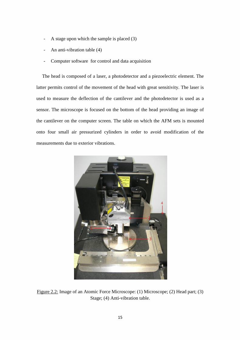
The AFM is composed of the following components (Figure 2.2):

- An optical microscope (1)

- A head with the AFM tip holder at its extremity (2)

15

- A stage upon which the sample is placed (3)

- An anti-vibration table (4)

- Computer software for control and data acquisition

The head is composed of a laser, a photodetector and a piezoelectric element. The

latter permits control of the movement of the head with great sensitivity. The laser is

used to measure the deflection of the cantilever and the photodetector is used as a

sensor. The microscope is focused on the bottom of the head providing an image of

the cantilever on the computer screen. The table on which the AFM sets is mounted

onto four small air pressurized cylinders in order to avoid modification of the

measurements due to exterior vibrations.

Figure 2.2: Image of an Atomic Force Microscope: (1) Microscope; (2) Head part; (3)

Stage; (4) Anti-vibration table.

16

2.2.1.2. AFM operation

The concept of the AFM is based on electrostatic interactions. A sharp tip mounted

on a cantilever approaches the sample surface and interactions appear between the

atoms on the surface and those at the end of the tip. Hence, the cantilever is deflecting

due to these interactions following Hooke’s law:

F = -kx (1)

where F is the force between the tip and the sample, k is the spring constant of the

cantilever, and x is the cantilever deflection.

Far from the surface interactions are weak, and the cantilever does not deflect. As

the tip gets closer to the surface, electrostatic forces start to appear (attractive or

repulsive forces) and the cantilever deflects. When the tip gets very close to the

surface and “touches” it, repulsive electrostatic interactions make the cantilever to

retract. The deflection of the cantilever is measured with the use of a laser reflecting

from the cantilevers’ surface into a photodiode (Figure 2.3).

The AFM is mainly used with two different modes which are the “contact mode”

and the “tapping mode”. In contact mode, the force between the sample and the tip is

maintained constant, which means that the deflection of the cantilever is also constant.

A feedback loop holds the cantilever deflection constant by moving the piezoelectric

scanner in the vertical direction Z (Figure 2.4). Then, the vertical movement of the

piezoelectric scanner at each (x,y) point provides the topography of the surface.

17

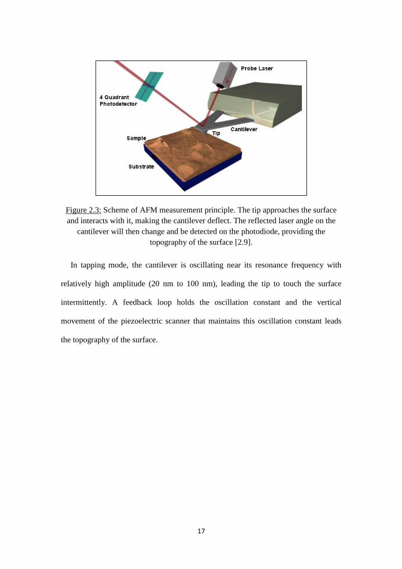
Figure 2.3: Scheme of AFM measurement principle. The tip approaches the surface

and interacts with it, making the cantilever deflect. The reflected laser angle on the

cantilever will then change and be detected on the photodiode, providing the

topography of the surface [2.9].

In tapping mode, the cantilever is oscillating near its resonance frequency with

relatively high amplitude (20 nm to 100 nm), leading the tip to touch the surface

intermittently. A feedback loop holds the oscillation constant and the vertical

movement of the piezoelectric scanner that maintains this oscillation constant leads

the topography of the surface.

18

Figure 2.4: A schematic representation of the Contact mode [2.10].

AFM can be performed in air or in liquid environment. When working in air, the

humidity of the environment may allow the formation of a thin water layer on the

surface of the specimen. Hence, a meniscus is formed between the tip and thin water

film on the surface, and it creates capillary forces bringing the tip and probe

downwards. Working in liquid environment allows the elimination of these capillary

forces, and it allows the reduction of Van der Waals' forces as well. AFM will provide

information about the chemical structure if using functionalized tips, or about

mechanical properties (adhesion, elasticity) if using the force-curve experiment. The

force-curve experiments create a force map by measuring the amount of force that the

cantilever feels when approaching the surface and then withdrawing.

AFM experiments were carried out in air (contact mode) on N. clavipes spider

dragline silk by other scientists. Samples were fixed on microscope slide using glue;

19

stretched and unstretched silk were prepared for analysis under dry conditions.

Longitudinal section of spider silks were analyzed as well as fiber cut at 45° and 90°

in the fiber direction axis [2.11].

Li et al. [2.11] demonstrated with the AFM that the silk is made of a core region

(containing two layers) surrounded by a thin skin. The fibrillar structure in the core

region is aligned along the fiber with pleated structure having a diameter varying from

100 nm to 300 nm. Shäfer et al. [2.12] proved that the spider silk surface exhibits

different structure, but in about all the samples a fibrillar structure oriented along the

fiber axis has been found.

A fibrillar structure on the surface of the Nephila pilipes and Latrodectus hesperus

(Black Widow) has also been demonstrated using AFM [2.13, 2.14]. About the fibrils

on the surface of the Black Widow, it has been demonstrated that they are decreasing

with increasing strain.

2.2.2. Electron microscopy

Scanning Electron Microscopy (SEM) is a technique used to see the topography of

a surface. A high-energy beam of electrons hits the surface and they interact with

atoms producing secondary electrons (SE) and backscattered electrons (BSE). These

electrons ejected from the surface of the specimen, captured by a photoelectric

element, contain information about the surface. The image is displayed by a cathode

ray tube; associated electronics then take a photo, as it is digitally displayed on a

computer screen.

20

The SEM function is pictured in Figure 2.5. Electrons are created by heating a

tungsten filament or a tip of LaB6 to a very high temperature. This filament emits free

electrons that are concentrated by a Wehnelt cylinder to form an electron beam. An

anode produces a high voltage differential that will accelerate the free electrons down

to the column. The electron beam passes through magnetic lenses that guide and focus

the beam on the sample. The scanning coils shift the beam in the x and y axes in order

to perform a raster scan of the surface. Hitting the surface produces electrons (SE or

BSE) that are collected by different detectors. SE or BSE detectors produce a signal

that is then converted into an image. The column and sample chamber is kept under

vacuum to maintain the integrity of the beam.

Figure 2.5: SEM operation. Electron beam is produced by the electron gun and is

guided towards the sample by passing through an anode and magnetic lenses.

Scanning coils drives the beam across the surface in a raster fashion and the SE and

BSE are collected by detectors [2.15].

21

SE electrons are electrons that come from the analyzed specimen. Beam electrons

interact with electrons in the atoms found on the specimen. Because electrons are

negatively charged, electrons from the beam and those from the specimen atoms will

repel each other. Hence, the specimen electrons will be ejected of the atom and exit

the specimen surface (inelastic scattering): these electrons are called secondary

electrons. Thus, they will be captured by a detector containing a positive charge on it.

BSE electrons are beam electrons that interact with the nucleus of specimen atoms.

Beam electrons go around the nucleus and exit the sample with the same speed

(elastic scattering). They move in straight lines and are collected by placing the

detector at the bottom of the column. These BSE are used to detect different atoms:

each type of atom has a different nucleus size and as the nucleus size increases the

number of BSE increases too. So heavy weight atoms will appear brighter than low

weight atoms.

To analyze a sample by SEM, it is preferred if the specimen is electrically

conductive to prevent the accumulation of charge on the surface that may cause

images artifacts. Therefore, insulating samples are coated with a metal, such as gold

or platinum. The coating is made by sputtering the metal on the surface of the

specimen in a high vacuum chamber.

Transmission Electron Microscopy (TEM) is another technique used for imaging

surfaces. The concept is almost the same as the SEM (Figure 2.6): an electron beam is

generated by a tungsten filament, goes through the anode and magnetic lenses, and

passes through the specimen. Two others magnetic lenses refocus the electron beam

and enlarge the image on a phosphorescent screen. In TEM, instead of looking at the

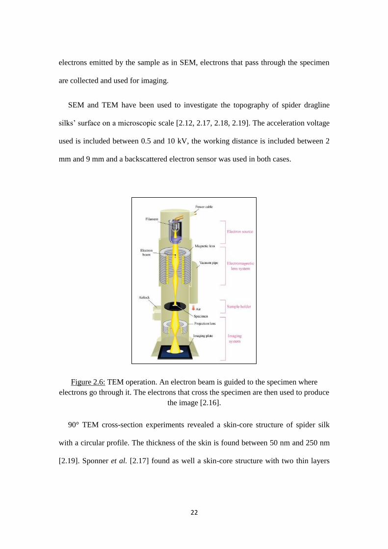
22

electrons emitted by the sample as in SEM, electrons that pass through the specimen

are collected and used for imaging.

SEM and TEM have been used to investigate the topography of spider dragline

silks’ surface on a microscopic scale [2.12, 2.17, 2.18, 2.19]. The acceleration voltage

used is included between 0.5 and 10 kV, the working distance is included between 2

mm and 9 mm and a backscattered electron sensor was used in both cases.

Figure 2.6: TEM operation. An electron beam is guided to the specimen where

electrons go through it. The electrons that cross the specimen are then used to produce

the image [2.16].

90° TEM cross-section experiments revealed a skin-core structure of spider silk

with a circular profile. The thickness of the skin is found between 50 nm and 250 nm

[2.19]. Sponner et al. [2.17] found as well a skin-core structure with two thin layers

23

on the skin, one being made of glycoproteins and the other one made of lipids that can

be easily removed.

SEM images revealed a smooth surface with a fibrillar structure. A coated layer is

also found on the skin with a variable thickness between 80 nm and 240 nm. Coating

the fiber with concavalin A lectin-gold complex (ConAAu15) for 30min at 295 °K

showed that the coated layer is made of glycoproteins homogeneously spread over the

surface [2.19]. SEM also allowed determining the diameter of the spider silk. While

different values have been reported [2.13, 2.17, 2.18], fiber diameter is essentially

found between three and five microns. The collection speed doesn’t play a role on the

mean diameter. It only plays a role on the maximum diameter found on a fiber: as the

collection speed increases, the maximum diameter increases [2.18].

2.2.3. Optical microscopy

Confocal laser scanning microscopy (CLSM) is another high-resolution image

technique for analyzing surfaces. Instead of using an electron beam as with SEM or

TEM, it utilizes a laser beam (Figure 2.7). This beam is focused on the specimen

surface by passing through the microscope objective lens. The emitted and scattered

laser light as well as any fluorescent light is collected by the same lens, and the lens

guides the laser light onto the detector by passing through a dichroic beam splitter. In

front of the light detector, there is a pinhole that blocks the light that is not coming

from the focal plane (the light which is out of focus is removed); hence, most of the

light is blocked resulting in better quality images at different depths. An emission

filter is also found before the light is collected by the photodetector, allowing the

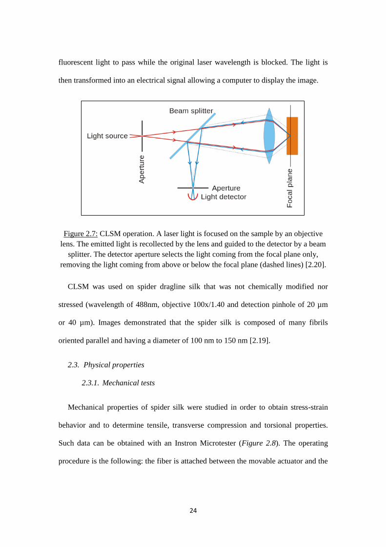
24

fluorescent light to pass while the original laser wavelength is blocked. The light is

then transformed into an electrical signal allowing a computer to display the image.

Figure 2.7: CLSM operation. A laser light is focused on the sample by an objective

lens. The emitted light is recollected by the lens and guided to the detector by a beam

splitter. The detector aperture selects the light coming from the focal plane only,

removing the light coming from above or below the focal plane (dashed lines) [2.20].

CLSM was used on spider dragline silk that was not chemically modified nor

stressed (wavelength of 488nm, objective 100x/1.40 and detection pinhole of 20 µm

or 40 µm). Images demonstrated that the spider silk is composed of many fibrils

oriented parallel and having a diameter of 100 nm to 150 nm [2.19].

2.3. Physical properties

2.3.1. Mechanical tests

Mechanical properties of spider silk were studied in order to obtain stress-strain

behavior and to determine tensile, transverse compression and torsional properties.

Such data can be obtained with an Instron Microtester (Figure 2.8). The operating

procedure is the following: the fiber is attached between the movable actuator and the

25

fixed load cell. Then, the fiber is tested whether in tensile or compression mode at a

specified rate until it breaks.

Figure 2.8: Instron Tester used for studying tensile properties [2.21].

Zemlin [2.3] tested tensile properties using a gauge length of 5.1 cm, a full scale

load of 2 g and a strain rate of 100 % per minute. Tests were carried out at 65 %

relative humidity and at a temperature of 21 °C. Results showed an average rupture

load of 1.26 g, a rupture tenacity of 0.9 GPa, a rupture elongation of about 18 % and

an initial modulus of about 11.8 GPa. Rupture elongation could go up to 30 % in

some cases. Furthermore, effect of collection speed on mechanical properties was also

studied; however, those data showed no specific trend.

26

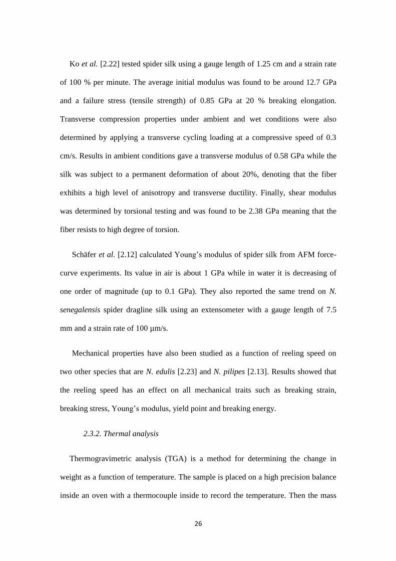
Ko et al. [2.22] tested spider silk using a gauge length of 1.25 cm and a strain rate

of 100 % per minute. The average initial modulus was found to be around 12.7 GPa

and a failure stress (tensile strength) of 0.85 GPa at 20 % breaking elongation.

Transverse compression properties under ambient and wet conditions were also

determined by applying a transverse cycling loading at a compressive speed of 0.3

cm/s. Results in ambient conditions gave a transverse modulus of 0.58 GPa while the

silk was subject to a permanent deformation of about 20%, denoting that the fiber

exhibits a high level of anisotropy and transverse ductility. Finally, shear modulus

was determined by torsional testing and was found to be 2.38 GPa meaning that the

fiber resists to high degree of torsion.

Schäfer et al. [2.12] calculated Young’s modulus of spider silk from AFM force-

curve experiments. Its value in air is about 1 GPa while in water it is decreasing of

one order of magnitude (up to 0.1 GPa). They also reported the same trend on N.

senegalensis spider dragline silk using an extensometer with a gauge length of 7.5

mm and a strain rate of 100 µm/s.

Mechanical properties have also been studied as a function of reeling speed on

two other species that are N. edulis [2.23] and N. pilipes [2.13]. Results showed that

the reeling speed has an effect on all mechanical traits such as breaking strain,

breaking stress, Young’s modulus, yield point and breaking energy.

2.3.2. Thermal analysis

Thermogravimetric analysis (TGA) is a method for determining the change in

weight as a function of temperature. The sample is placed on a high precision balance

inside an oven with a thermocouple inside to record the temperature. Then the mass

27

change is measured as the temperature is increased. During the thermal treatment, the

mass of samples changes because of dehydration, oxidation or decomposition.

TGA was performed on spider silk and showed that the fiber is stable below 230

°C. A major decomposition occurs between 230 °C and 440 °C with a loss of

approximately 52 % weight [2.18].

Dynamic mechanical analysis (DMA) is a useful technique to study the

viscoelastic behavior of materials. This method allows the determination of the

dynamic modulus under vibratory conditions: a sinusoidal stress is applied to the

sample and the strain is recorded.

The dynamic modulus is decomposed in two parts following the equation:

where represents the storage modulus (elastic behavior of material) and

represents the loss modulus (viscous behavior of material). Two different modes can

be used: the “temperature sweep mode” where the frequency of the sinusoidal stress is

constant and the measure of dynamic modulus is done as the temperature changes;

and the “frequency sweep mode” where the dynamic modulus is recorded at fixed

temperature with a change in frequency.

DMA was performed on spider silk with a first thermal cycle: temperature of

heating up to 180 °C and maintained at this temperature for 30min. The second

thermal cycle was performed until the Young’s modulus was completely lost (which

occurred around 220 °C). From these two runs, two transitions can be seen: one at 70

28

°C being attributed to some transition in the amorphous domain, and another one at

210 °C representing the motion of the chains associated with partial melt [2.18].

Thermomechanical analysis (TMA) is another method of thermal analysis. As

constant force (constant stress) is applied to the fiber by hanging a weight on the

material and while the temperature is also maintained constant, the initial change in

strain is measured.

TMA experiments were carried out on spider silk at four temperatures (-40, 25,

100 and 150 °C) with an initial fiber length of 2.54 cm and a constant stress of 1 N

applied. A strong dependence of the initial strain was observed as a function of the

temperature, with the initial strain increasing with temperature. But once the fiber has

been initially elongated, the strain did not change anymore [2.18].

29

CHAPTER THREE

INVESTIGATION OF SPIDER DRAGLINE SILK SURFACE MORPHOLOGY

Spider dragline silk surface has not been investigated intensively and only few

studies have been reported (see Section 2.2). Surface study will give an insight in the

morphology and will allow us to determine if there is any structural pattern, such as

seen in the core with the fibrils. Thus, we will investigate the surface morphology of

the spider dragline silk using AFM, specifically the surface roughness. Surface

roughness is important during fiber production, and since one goal of this thesis is to

help people design and synthesize a fiber similar to spider silk, we will investigate

roughness as a function of collection speed. In this chapter, the methods used to

prepare the sample for AFM experiment and the designs for roughness experiments

will be described.

3.1. Materials and Methods

3.1.1. Spider silk

3.1.1.1. Collection

The dragline silk from N. clavipes was collected with the use of a take-up reel on

a spool (left picture on Figure 2.1). The spider was sedated by placing in a

refrigerator for one hour at 4 °C and then put rapidly onto a Styrofoam block and

attached with curved staples around her legs and body (right picture on Figure 3.1).

Once she was tightened, she was put under a microscope and forceps were brought

into proximity of the spinnerets to extract the silk. As seen on Figure 3.2, two dragline

silk fibers can be pulled out of the spinnerets at the same time and, if they are seen,

they need to be separated. Then, the fiber was put onto the spool ready to be reeled.

30

Different speeds of collection were used based on the voltage applied (1V =1.4 cm.s-1

,

3 V = 4.2 cm.s-1

).

Figure 3.1: (Left) Picture of a take-up reel with (1) the spool and (2) the reeling

motor. (Right) Picture of a N. clavipes spider stapled onto a Styrofoam block in order

to extract silk from her spinnerets (Photo credit: Janci Despain).

In this part of the project, spider silk was collected at speeds of 0.72, 2.16, 14.0,

45.7 and 65.1 mm.s-1

for analysis. These speeds were collected by previous people in

the group (except for the one at 14 mm.s-1

), and we will be able to study later the

roughness as a function of a broad range of collection speed. Each spider silk sample

Figure 3.2: Relevant anatomy of the

spinnerets. (1) Anterior lateral spinneret

that houses one major ampullate spigot on

its underside. (2) Major ampullate spigot

that produces dragline silk. One major

ampullate spigot is located on the

underside of each anterior lateral

spinneret. (3) Dragline silks produced by

each major ampullate spigot. (Photo

Credit: Janci Despain)

31

was stored in air in a closed plastic pill bottle, in a dark cabinet at room temperature

and humidity after collection.

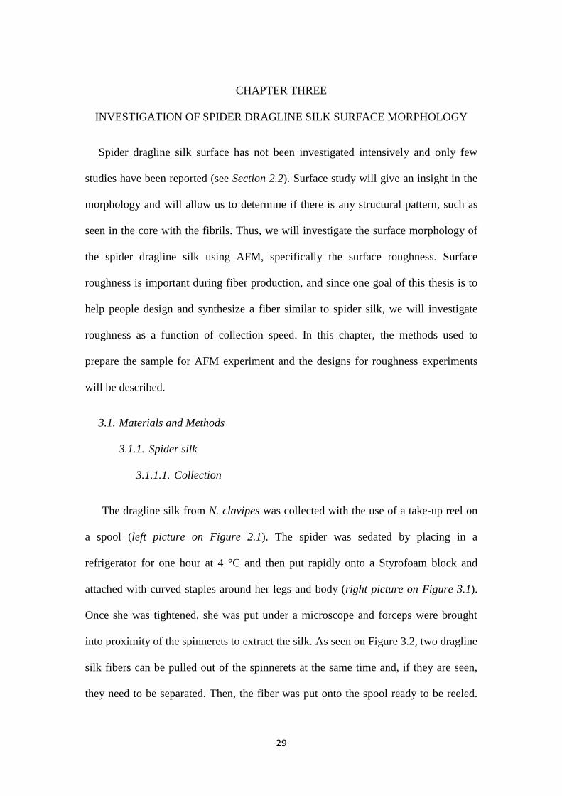
3.1.1.2. Sample preparation

To mount the spider silk, the necessary supplies include: a microscope slide, nitrile

gloves, cyanoacrylate adhesive (Loctite® Super Glue) and two hands. While wearing

the gloves, two points of glue on the middle of the microscope slide were spread.

Spider silk was then stretched and held on the glue until it stuck. The compliance of

the fiber was minimized by putting glue points along the fiber, providing also many

spots to analyze (Figure 3.3). Once the samples have been prepared, they were left in

air letting the glue dry during the night and AFM was performed later. Another reason

for putting several glue points on the spider silk is that when the fiber is only stuck at

its ends, it moves when trying to take an image with the AFM resulting in very bad

images. Thus, closed glue points give more stability.

Figure 3.3: Two spider silk fibers mounted on a microscope slide. The fibers are

difficult to see on this picture since they are very thin. The dots of glue indicate

the path of the fibers.

32

3.1.2. Atomic Force Microscope

A standard Atomic Force Microscope (Veeco Dimension 3100, Digital

Instruments) with an internal optical microscope was used. Cantilevers made of non-

conductive silicon nitride with gold and chrome coating on the front- and back-side

were utilized. The radius of the tip has been previously determined by SEM to be

about 50nm. The spring constant of the cantilever is about 0.12 N/m with a resonant

frequency between 14 Hz and 26 Hz. The AFM was used in contact mode in a fluid

environment (0.01 M of Phosphate Buffer Saline) for every experiment. Images are

taken with 512 data points per line over 512 lines. For each speed analyzed, 42

images were taken.

3.2. Experimental design

3.2.1. Roughness experiment

N. clavipes dragline silk was investigated by AFM in air and then in fluid using

contact mode. Spider silks collected by previous scientists at speeds of 0.72, 2.16,

45.7 and 65.1 mm.s-1

, and by me at speed of 14.0 mm.s

-1, were analyzed. Fresh spider

silk and five years old spider silk were investigated. No chemical treatment was done

on the silk before analyzing it.

Once the images are captured with the AFM, the images are filtered with a

flattening process. The “Planefit” command is used to remove image artifacts caused

by tilt or bow. It calculates a single polynomial fit for the entire image and then

subtracts this polynomial fit from the image. Three different polynomial fit can be

applied (1st, 2

nd and 3

rd order polynomial fit), each of them having a different effect on

the image (Table 3.1) [3.1]. In our case, a 2nd

order fit is applied to the entire image

33

(in the X and Y directions) in order to remove the arch shaped bow due to the fiber

curvature.

Table 3.1: Three different orders of flattening and their effect on the image.

1st order flatten 2

nd order flatten 3

rd order flatten

Removal of the

tilt on the image

Removal of the

arch shaped bow

Removal of the

S-shaped bow

After the planefitting processing, we can extract the mean roughness value (Ra)

from each image. The Ra value represents the arithmetic average of the deviations

from the center plane and is calculated with the following formula:

(3)

where Zcp is the Z value of the center plane, Zi is the actual Z value and N is the

number of points in the image. It is important to notice that the Planefit process

previously done on the image may affect the roughness values. When roughness

analysis is performed by the software, the roughness values are calculated according

to the relative height of each pixel in the image; and when the Planefit process is

applied to the image it reorients these pixels. Hence, the height of these pixels may

have changed, modifying the roughness value. Also, roughness values are influenced

by the size of the scanned area. Roughness values increase with increasing the

scanned surface area [3.2].

34

3.2.2. Verifying that AFM scanning of surface is a nondestructive technique

The force between AFM tips and soft samples can caus the formation of wear

tracks. The purpose of this experiment is to confirm that the selected AFM set point

was not causing deformation of the spider dragline silk. The protocol for our

experiment was to put the tip on a spot, and let it take five images in a row of this

same spot (without retracting the tip). These images were taken with a scan size of 1

µm x 1 µm. Following this, the same experiment was done with enlarging the size of

the surface analyzed to 2 µm x 2 µm, still without retracting the tip. If a significant

modification in roughness is seen or an internal wear box is detected, then we will be

able to conclude that we are scraping the surface. By scanning the same area but on a

bigger scale, we will be able to see if we can match the small scanned area into the

bigger one; also, we will be able to see if enlarging the size of the scan causes an

increase in roughness. Also, a same type of experiment was carried out by taking

eleven images in a row on the same spot in order to see if by going a little bit longer

on the same area we still not scrape it.

3.2.3. Average roughness repeatability experiment

Results from the scrape checking experience suggested that the repeatability of the

experiments must be studied. The repeatability was studied to see if an experiment

can be done again under the same conditions and by the same instrument without

variations in measurements. In our case, we wanted to see if there was any variation

in roughness measurements when we carried out an experiment on a spider silk fiber.

An example for studying the repeatability would be to move the tip on ten different

spots on the fiber, take an image at each spot and calculate the average roughness for

35

these ten spots; and then move again the tip on this ten same spots, take an image and

recalculate the average roughness. Having a look at the average roughness differences

will give us the information on repeatability. In our case, it is impossible to do it this

way because after removing the tip from one spot it is impossible to relocate this same

spot. So the repeatability has been studied by using another protocol. This protocol

consists of taking three images in a row on the same spot at seven different spots

along the fiber (Figure 3.4). Each row corresponds to an experiment done as if we

were following the protocol in the previous example. Thus, the repeatability of the

experiments will be studied by analyzing the average roughness variations of these

rows.

Figure 3.4: Schematic representation of the experiment. The spider silk fiber is

represented with the cylindrical shape and the squares represent one image taken

on one spot. Each column (A, B, C…) corresponds of a series of 3 images taken

on the same spot.

36

CHAPTER FOUR

CHARACTERIZATON OF THE AMINO ACIDS ON THE SURFACE OF SPIDER

DRAGLINE SILK

The bulk composition is known to have a pattern in its primary structure (i.e.,

amino acid sequence) having repeating blocks of alanine and glycine motifs. Amino

acid composition of the skin surface may have a different pattern than the core, and a

close look at the electrically charged amino acid will enable us to see: (1) if this type

of amino acid is present on the surface, (2) if the surface roughness is generated by

this type of amino acid, and (3) if a pattern in their spatial frequency is detected. In

this chapter will be found the methods and experimental design to accomplish these

objectives.

4.1. Materials and methods

4.1.1. Spider silk

The same type of spider dragline silks utilized in the roughness experiments, i.e.

from N. clavipes, were used to identify the amino acids on the silk surface. Fibers

collected at different speed were used and were at least five years old. Each spider silk

sample was stored in air in a closed plastic pill bottle, in a dark cabinet at room

temperature and humidity after collection. Fibers were mounted on a microscope slide

without being stretched. Natural spider dragline silk were used as well as fibers rinsed

with 70 % ethanol.

37

4.1.2. Labeling of carboxyl and amine groups with gold nanoparticles

Gold nanoparticles (Cytodiagnostics, 20nm diameter, particles per ml: 6.54×1011

)

were functionalized with carboxyl groups (respectively amine groups) in order to see

positively charged amino acids (respectively negatively charged amino acids). The

protocol used to link gold nanoparticles to amino acids is described in the following

paragraph. This protocol is a novel method of protein surface analysis, originally

applied to a wool fiber study [4.1]. The protocol was developed at Clemson

University by James Chow, a bioengineering undergraduate student, while

contributing to the thesis of Bonnie Zimmerman [4.2]. The ultimate goal of this

protocol is to create a stable amide bond between amino acids and gold nanoparticles.

The gold nanoparticles thus functionalized will be observable using backscatter SEM.

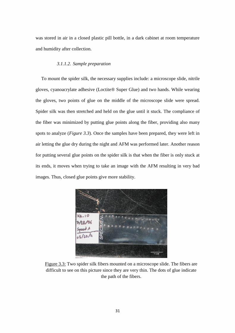
This discussion follows Figure 4.1. The compound 1-Ethyl-3-[3-

dimethylaminopropyl]carbodiimide (EDC) attaches to a carboxylic group from

molecule 1 to form an amine-reactive, o-acylisourea ester. This intermediate can react

directly with amine groups from molecule 2 to form a stable amide bond.

Nevertheless, this intermediate might hydrolyze in aqueous solution making it

unstable and short-lived. Hence, N-hydroxysulfosuccinimide (Sulfo-NHS) is added to

increase the stability of the intermediate as well as the resultant amide bond

formation, leading to an amine-reactive Sulfo-NHS ester. Finally, the Sulfo-NHS

leaves when the amine group from molecule 2 is able to react with the carboxylic

group from molecule 1, and this leads to a stable amine bond between molecules 1

and 2.

38

Figure 4.1: Reaction used for attaching functionalized gold nanoparticles to the

specific charged amino acids on the spider dragline silk surface [4.3].

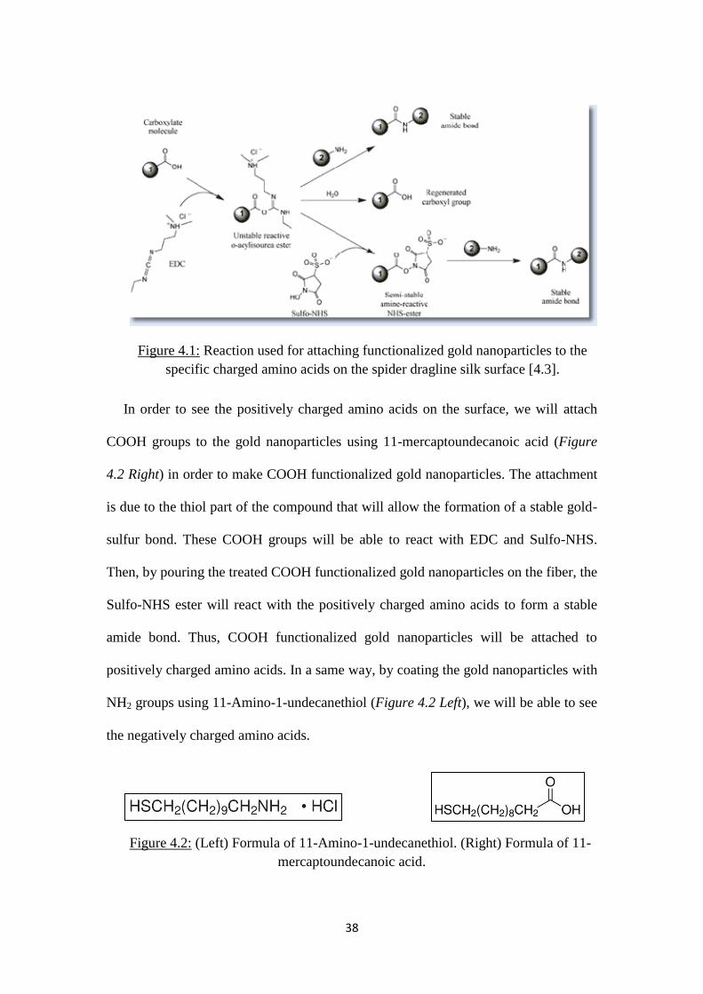
In order to see the positively charged amino acids on the surface, we will attach

COOH groups to the gold nanoparticles using 11-mercaptoundecanoic acid (Figure

4.2 Right) in order to make COOH functionalized gold nanoparticles. The attachment

is due to the thiol part of the compound that will allow the formation of a stable gold-

sulfur bond. These COOH groups will be able to react with EDC and Sulfo-NHS.

Then, by pouring the treated COOH functionalized gold nanoparticles on the fiber, the

Sulfo-NHS ester will react with the positively charged amino acids to form a stable

amide bond. Thus, COOH functionalized gold nanoparticles will be attached to

positively charged amino acids. In a same way, by coating the gold nanoparticles with

NH2 groups using 11-Amino-1-undecanethiol (Figure 4.2 Left), we will be able to see

the negatively charged amino acids.

Figure 4.2: (Left) Formula of 11-Amino-1-undecanethiol. (Right) Formula of 11-

mercaptoundecanoic acid.

39

4.1.3. Sample preparation

The preparation of the spider dragline silk on the microscope slide is the same as

for the AFM study except that the silk is only glued at its ends and not all along the

fiber. To attach the functionalized gold nanoparticles on the surface of the fiber, the

steps shown in Figure 4.3 are followed.

Figure 4.3: Steps preparation for attaching gold nanoparticles functionalized with

COOH groups to the negatively charged amino acids. A switch between 11-Amino-1-

undecanethiol and 11-mercaptoundecanoic acid needs to be done to attach gold

nanoparticles to the positively charged amino acids.

4.1.4. Scanning electron microscopy

A Hitachi SU6600 scanning electron microscope was used to analyze the spider

dragline surface and also to identify the amino acids on the surface. Both SE and BSE

detectors are attached to the machine and are used for a different purpose: SE detector

was for analyzing the fiber surface while BSE detector was used for identifying the

amino acids with attached gold nanoparticles.

Microscope slides were mounted on a stub with double sided adhesive carbon tape,

and samples without gold nanoparticles were coated with platinum Pt in a 15 mA

40

sputter coater (Hummer™ 6.2). SEM photomicrographs were taken at working

distances of 9 mm to 10 mm using an electron beam acceleration voltage of 15 kV or

20 kV, and with a variable pressure environment to reduce charging effect. Using the

backscatter detector of the SEM, gold nanoparticles were easily identified as they

appeared much brighter. Since gold has a higher atomic number compared to the

atoms on the spider dragline silk surface, they reflect more strongly the electrons.

4.2. Experimental design

The purpose of this experiment is to determine if negatively/positively charged

amino acids are found on the surface of the spider dragline silk. The different type of

amino acids found in spider dragline silk, as well as their properties, is reported in

Table 2.1. The structure of all these amino acids is given in the appendix B.

We can see from Table 2.1 that the amount of positively charged amino acids

found in spider silk (~4 % total) is less than the amount of negatively charged amino

acids (~10 % total). Even if the spider dragline silk does not contain a high amount of

positively or negatively charged amino acids, it should still be possible to see most of

them. Indeed, it is most likely to find charged amino acids on the surface of a protein

because it is energetically more stable to be at the surface rather than in the core,

where the environment is neutral (hydrophobic).

However, it is important to note that a lipid layer may be present on the surface at

some locations [4.4]. Lipids are not made of amino acids; in fact, they will prevent us

from seeing the amino acids we are looking for on the surface because the amino

acids will be below this lipid coating. Thus, it will be necessary to remove this lipid

41

layer by washing the samples with alcohol or ether before doing the particle

treatment.

Furthermore, from previous work done on spider dragline silk, a layer containing

glycoprotein has been found underneath the lipid layer, showing these glycoproteins

spread homogeneously on the surface [4.4, 4.5]. Glycoproteins are proteins containing

oligosaccharide chains also called glycans (carbohydrate/sugar), which are covalently

bond to polypeptide chains. Oligosaccharide chains are bonded to peptide chains by

two types of linkage to form a glycoprotein [4.6]:

N-linkage: the oligosaccharide chain is linked to the nitrogen atom found in

the side-chain of the amino acid asparagine.

O-linkage: the oligosaccharide chain is linked to the oxygen atom found in the

side-chain of the amino acids serine or threonine (Figure 4.4).

Thus, glycoproteins are oligosaccharide chains attached to the polypeptide chains

of spider silk. Hence, these sugar chains will point toward the surface and will

contribute to the spider silk surface. These glycoproteins don’t hide the amino acids

we are looking for since they are attached to asparagine or serine/threonine; but the

bulky carbohydrate chains might be large enough to prevent gold nanoparticles to

target the amino acids we are interested in, if located next to them.

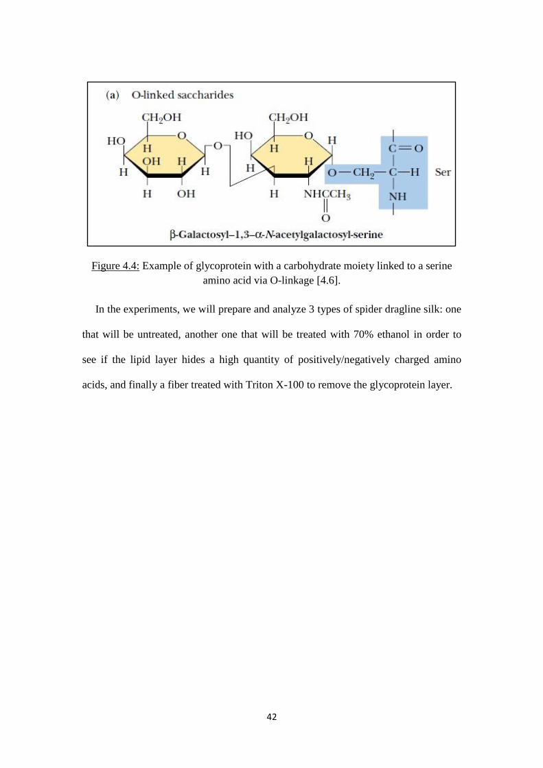
42

Figure 4.4: Example of glycoprotein with a carbohydrate moiety linked to a serine

amino acid via O-linkage [4.6].

In the experiments, we will prepare and analyze 3 types of spider dragline silk: one

that will be untreated, another one that will be treated with 70% ethanol in order to

see if the lipid layer hides a high quantity of positively/negatively charged amino

acids, and finally a fiber treated with Triton X-100 to remove the glycoprotein layer.

43

CHAPTER FIVE

RESULTS

5.1. Roughness

Among all the images taken, different surface features were observed but most of

the time we obtained a rough surface (Figure 5.1 and Figure 5.2). A complete

representation of images can be found in Appendix D.

The roughness values from Figure 5.1 and 5.2 cannot be compared since the size of

the scan is different for each image. Among all fibers analyzed, the roughness values

of each image are between 20 nm and 100 nm, approximately. On the other hand,

since the roughness is changing a lot along a fiber, the standard deviation of each fiber

is found to be high, around 30 nm.

Figure 5.1: Height and deflection image of N. clavipes spider dragline silk reeled up at

2.16 mm.s-1

analyzed on 08/16/2011 in air. The size of the image is 4 µm x 2 µm. The

surface roughness is 63.1 nm.

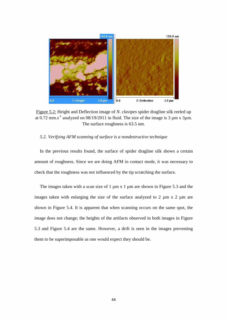
44

Figure 5.2: Height and Deflection image of N. clavipes spider dragline silk reeled up

at 0.72 mm.s-1

analyzed on 08/19/2011 in fluid. The size of the image is 3 µm x 3µm.

The surface roughness is 63.5 nm.

5.2. Verifying AFM scanning of surface is a nondestructive technique

In the previous results found, the surface of spider dragline silk shows a certain

amount of roughness. Since we are doing AFM in contact mode, it was necessary to

check that the roughness was not influenced by the tip scratching the surface.

The images taken with a scan size of 1 µm x 1 µm are shown in Figure 5.3 and the

images taken with enlarging the size of the surface analyzed to 2 µm x 2 µm are

shown in Figure 5.4. It is apparent that when scanning occurs on the same spot, the

image does not change; the heights of the artifacts observed in both images in Figure

5.3 and Figure 5.4 are the same. However, a drift is seen in the images preventing

them to be superimposable as one would expect they should be.

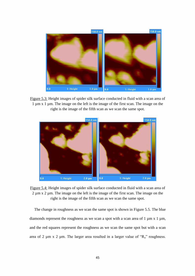
45

Figure 5.3: Height images of spider silk surface conducted in fluid with a scan area of

1 µm x 1 µm. The image on the left is the image of the first scan. The image on the

right is the image of the fifth scan as we scan the same spot.

Figure 5.4: Height images of spider silk surface conducted in fluid with a scan area of

2 µm x 2 µm. The image on the left is the image of the first scan. The image on the

right is the image of the fifth scan as we scan the same spot.

The change in roughness as we scan the same spot is shown in Figure 5.5. The blue

diamonds represent the roughness as we scan a spot with a scan area of 1 µm x 1 µm,

and the red squares represent the roughness as we scan the same spot but with a scan

area of 2 µm x 2 µm. The larger area resulted in a larger value of “Ra” roughness.

46

Also an increase in roughness with scan number was found when scanning the 1 µm x

1 µm area, and a decrease with scan number was found when scanning the 2 µm x 2

µm area.

Figure 5.6 shows another study of scrape checking as scanning a same spot eleven

times in a row. The roughness was found to vary only a few nanometers.

Figure 5.5: Roughness changes with scanning a same spot with a scan area of 1 µm x

1 µm (blue diamonds) and with scanning the same area but with a scan size of 2 µm x

2 µm (red squares).

40

50

60

70

80

90

100

110

0 1 2 3 4 5 6

Ro

ugh

ne

ss (

nm

)

Scan number

Roughness differencies as scanning on a same spot 5 times

Scan 1x1µm

Scan enlargement 2x2µm

47

Figure 5.6: Roughness changes with scanning the same spot eleven times in a row.

5.3. Average roughness repeatability

The drift seen in the images of section 4.2., suggests that the repeatability of the

experiments must be studied. The protocol consisted of taking 3 images on the same

spot at seven different spots along the fiber (Figure 3.8). The results of average

roughness are summarized in Table 5.1. Normally, the standard deviation of each

column should be equals to zero since we are scanning the same spot (the images

should not change at all). But it has been seen in the scrape checking experiments that

there is a current drift; apparently, the drift is modifying the roughness resulting in a

non null standard deviation.

What it is interesting to underline is that the average roughness is not changing

significantly. It doesn’t increase or decrease by half of its value, and there is no trend

observed between each row (such as constant increase or decrease).

50

51

52

53

54

55

56

57

58

0 2 4 6 8 10 12

Ro

ugh

ne

ss (

nm

)

Scan number

Roughness differencies as scanning on a same spot 11 times

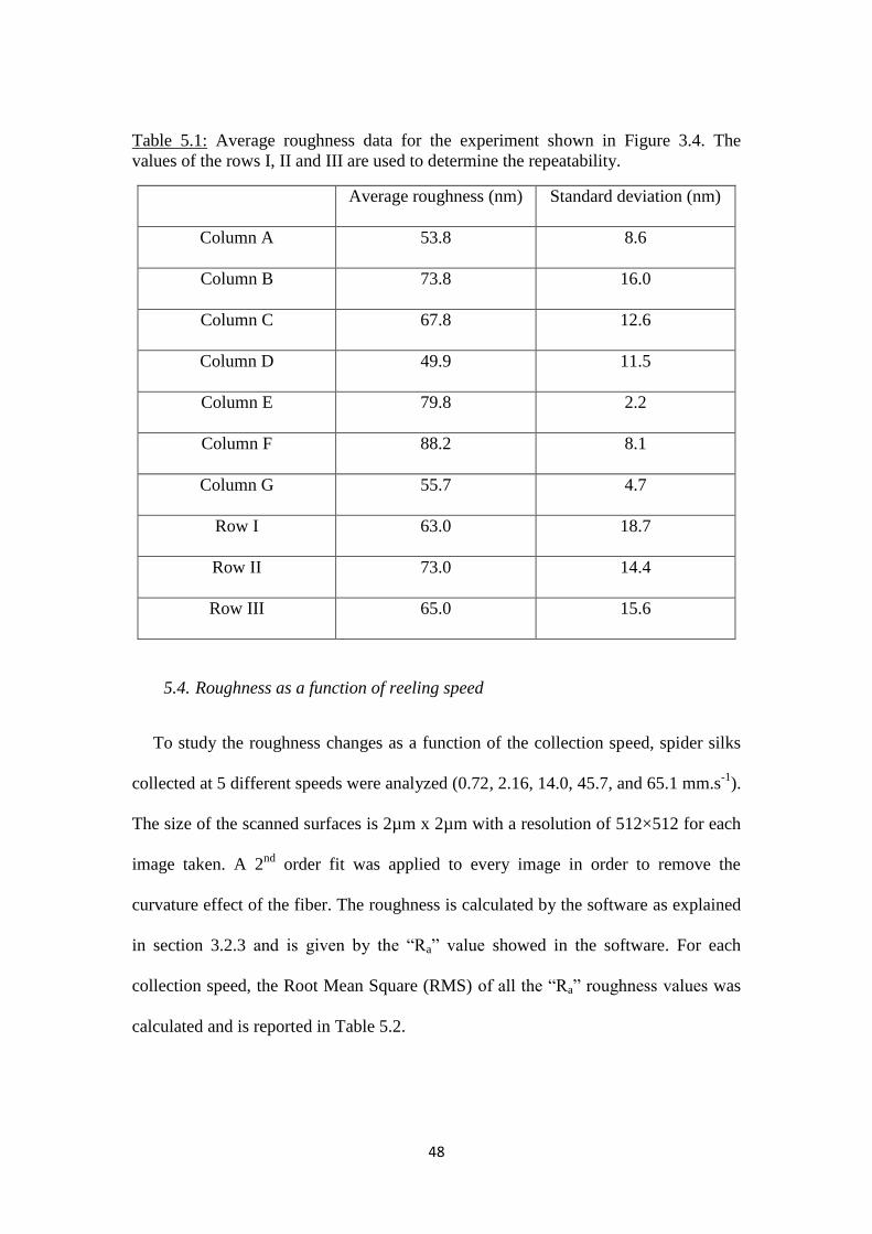
48

Table 5.1: Average roughness data for the experiment shown in Figure 3.4. The

values of the rows I, II and III are used to determine the repeatability.

Average roughness (nm) Standard deviation (nm)

Column A 53.8 8.6

Column B 73.8 16.0

Column C 67.8 12.6

Column D 49.9 11.5

Column E 79.8 2.2

Column F 88.2 8.1

Column G 55.7 4.7

Row I 63.0 18.7

Row II 73.0 14.4

Row III 65.0 15.6

5.4. Roughness as a function of reeling speed

To study the roughness changes as a function of the collection speed, spider silks

collected at 5 different speeds were analyzed (0.72, 2.16, 14.0, 45.7, and 65.1 mm.s-1

).

The size of the scanned surfaces is 2µm x 2µm with a resolution of 512×512 for each

image taken. A 2nd

order fit was applied to every image in order to remove the

curvature effect of the fiber. The roughness is calculated by the software as explained

in section 3.2.3 and is given by the “Ra” value showed in the software. For each

collection speed, the Root Mean Square (RMS) of all the “Ra” roughness values was

calculated and is reported in Table 5.2.

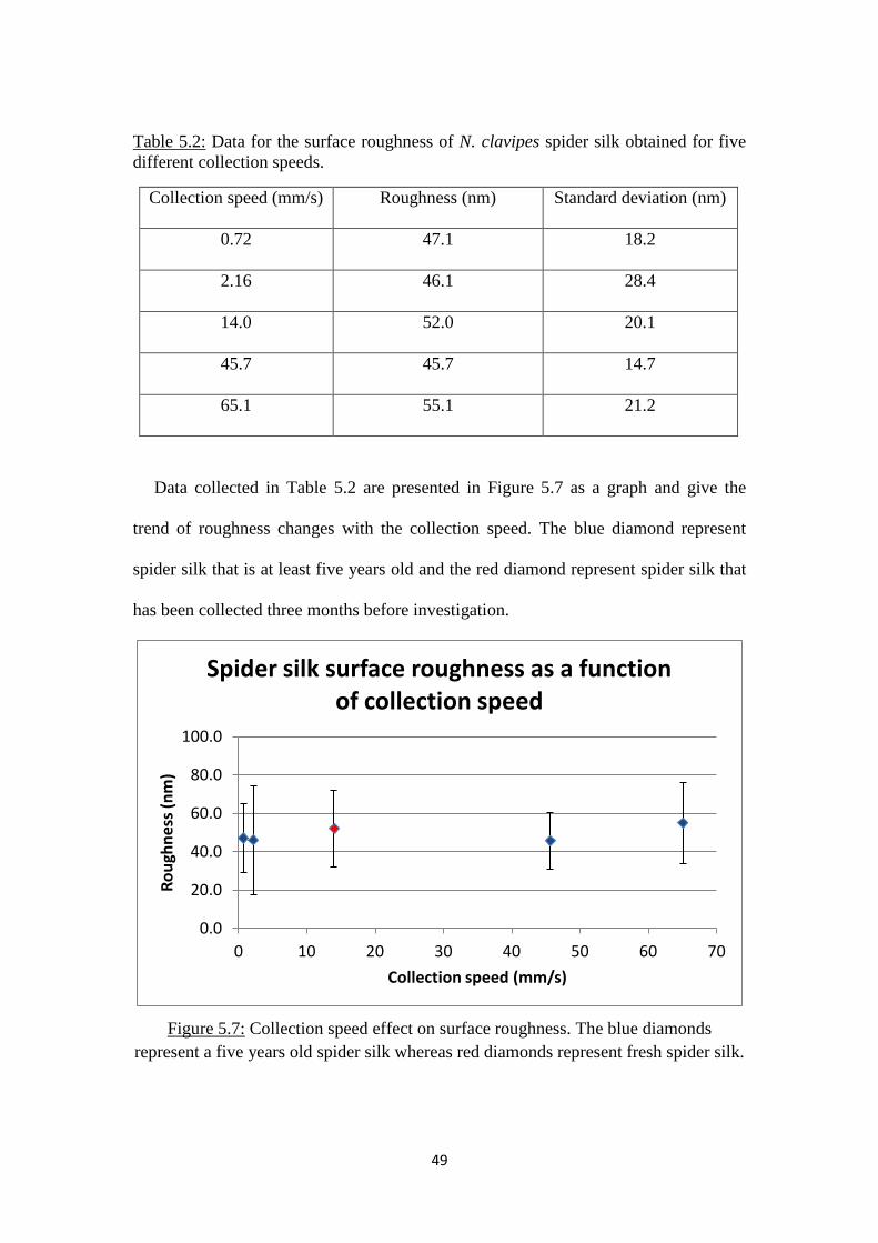
49

Table 5.2: Data for the surface roughness of N. clavipes spider silk obtained for five

different collection speeds.

Collection speed (mm/s) Roughness (nm) Standard deviation (nm)

0.72 47.1 18.2

2.16 46.1 28.4

14.0 52.0 20.1

45.7 45.7 14.7

65.1 55.1 21.2

Data collected in Table 5.2 are presented in Figure 5.7 as a graph and give the

trend of roughness changes with the collection speed. The blue diamond represent

spider silk that is at least five years old and the red diamond represent spider silk that

has been collected three months before investigation.

Figure 5.7: Collection speed effect on surface roughness. The blue diamonds

represent a five years old spider silk whereas red diamonds represent fresh spider silk.

0.0

20.0

40.0

60.0

80.0

100.0

0 10 20 30 40 50 60 70

Ro

ugh

nes

s (n

m)

Collection speed (mm/s)

Spider silk surface roughness as a function of collection speed

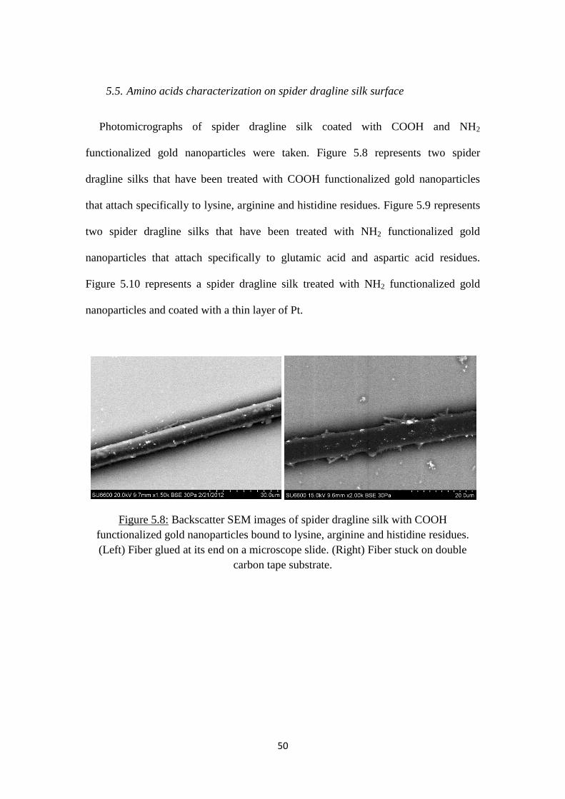
50

5.5. Amino acids characterization on spider dragline silk surface

Photomicrographs of spider dragline silk coated with COOH and NH2

functionalized gold nanoparticles were taken. Figure 5.8 represents two spider

dragline silks that have been treated with COOH functionalized gold nanoparticles

that attach specifically to lysine, arginine and histidine residues. Figure 5.9 represents

two spider dragline silks that have been treated with NH2 functionalized gold

nanoparticles that attach specifically to glutamic acid and aspartic acid residues.

Figure 5.10 represents a spider dragline silk treated with NH2 functionalized gold

nanoparticles and coated with a thin layer of Pt.

Figure 5.8: Backscatter SEM images of spider dragline silk with COOH

functionalized gold nanoparticles bound to lysine, arginine and histidine residues.

(Left) Fiber glued at its end on a microscope slide. (Right) Fiber stuck on double

carbon tape substrate.

51

Figure 5.9: Backscatter SEM images of spider dragline silk with NH2 functionalized

gold nanoparticles bound to glutamic acid and aspartic acid residues. (Left) Fiber

fixed on double coated carbon tape and stretched. (Right) Fiber glued at its end on a

microscope slide.

Figure 5.10: Backscatter SEM images of a spider dragline silk with NH2

functionalized gold nanoparticles bound to glutamic acid and aspartic acid residues

coated with a thin layer of Pt.

Figure 5.11 represents a bundle of spider dragline silk with COOH functionalized

gold nanoparticles that attach specifically to lysine, arginine and histidine residues.

Figure 5.12 represents a bundle of spider dragline silk with NH2 functionalized gold

nanoparticles that attach specifically to glutamic acid and aspartic acid residues.

52

Figure 5.11: Backscatter SEM images of a bundle of spider dragline silks fixed on

double carbon tape substrate with COOH functionalized gold nanoparticles bound to

lysine, arginine and histidine residues.

Figure 5.12: Backscatter SEM images of a bundle of spider dragline silks fixed on

double carbon tape substrate with NH2 functionalized gold nanoparticles bound to

glutamic acid and aspartic acid residues.

53

CHAPTER SIX

DISCUSSION

First of all, results in section 5.2 demonstrate that the roughness wasn’t influenced

by the tip scraping the surface. Indeed, the overall images remained the same when

scanning the same spot and there was no significant change in roughness as seen in

Figure 5.5 and Figure 5.6. However, we would have expected the roughness to stay

constant as we scan the same spot many times. In Figure 5.5 and Figure 5.6, this is not

the case. This variation in roughness is due to the drift seen between images. It

slightly changes the appearance of the image, including and/or excluding rough

features, hence modifying the calculated roughness. Moreover, results obtained in

section 5.3 for testing the repeatability showed that under the same experimental

conditions the variations of measurements are negligible and that one image per spot

will be sufficient.

Among all the images taken, the N. clavipes spider dragline silk surface showed

different structures along the fiber and it was found to be rough. An important thing to

notice is that when seeing the fiber under the optical microscope of the AFM we

could see sometimes that the fiber surface had black marks on it. It is unlikely that

these were part of the surface in that they were very big and distinguishable, so it is

thought that the surface was contaminated at these places. Hence, great care was taken

to not perform a measurement around these black marks. In a same way, glue may

have been contaminating the fiber surface next to the glue points; thus, no

measurements were carried out around the glue points. Different locations on the

spider silk exhibited different roughness varying in the range of 20 nm to 100 nm.

54

From Figure 5.1 and 5.2, it is seen that there are some blobs with a high height laying

down on the surface. Sponner et al. [6.1] showed that a lipid/glycoprotein layer can be

found at the surface of the silk; since no chemical treatment was applied to our

samples, these blobs might correspond to lipids or glycoproteins. Furthermore, it has

been noticed on many images that there is some cracks on the surface oriented along

the fiber axis (like the black “worm” lines on Figure 5.2). Since the spider silk is

known to have a skin-core structure with fibrils inside the core [6.2], this crack could

be thought to be in fact a fibril. However, if we were able to see the fibrils, we would

see many fibrils that compose the core and not only one, so this is not a likely

explanation. Moreover, a skin cladding surrounds the core [6.1] and this would

prevent the AFM from seeing the core. Thus, a possible explanation is that this outer

skin may be releasing some stress by forming these cracks. Since the fiber is

stretched, both during the silking operation and during sample preparation, this

cracking may be a result of stretching the fiber above its yield elongation point

sometime during the sample preparation. This could correlate with the results of Zax

et al. [6.3] who found that a splitting was occurring along and across the fiber axis

after tensile testing.

Also, spider silk is known to exhibit a supercontraction effect that is related to the

proline content of MaSp2. Jelinski et al. [6.4] showed that spider silk shrinks in length

when put under water, but that was observed when the fiber was attached only to one

end. In our study, the fiber is analyzed between two points of glue preventing it to

shrink. Nevertheless, the supercontraction effect due to the PBS environment might

induce some stress in the fiber and make it crack on the surface. It is also possible that

55

these surface features are a normal aspect of the silk. Much additional work would be

required to settle this question.

Comparison with a paper from Schäfer et al. [6.5] showed no correlation between

images. Their images were taken with the same scan size as in this thesis, i.e. 2 µm x

2 µm, and the fibrillar type structure they found is not present in any of our images. A

possible explanation is that the samples analyzed in this study are at least five years

old, and the spider silk surface might have aged during that time, changing the

structure of the surface. But since roughness experiments performed on fresh spider

dragline silk did not show any changes in roughness or in morphology, this is not a

likely explanation.

Study of the surface roughness as a function of the collection speed presented in

section 5.4 showed no trend. According to the error bars, it is seen that surface

roughness values are included in the same range of values and no significant deviation

is reported. It is important to notice that the roughness values may not be the “exact”

values because of the scan size area used and also because of the Planefit process used

to remove the arch shaped bow on the images. However, since every image was taken

with the same scan size of 2 µm x 2 µm and was treated with a 2nd

order planefitting,

the trend reported here is valid.

Roughness values might also be affected by the fact that the fiber is stretched. By

stretching the fiber, we don’t change the amino acid content on the surface of the fiber

but we may stretch the polypeptide bonds and change the conformation of the amino

acids. Stretching effect on crystals’ size was previously studied by Grubb et al. [6.6],

showing that the extension of the fiber resulted in an increase of crystal orientation:

56

polypeptide chains are more aligned along the fiber and the lateral size of the crystals

is decreasing of less than 1nm. These results concern the crystals in the core of the

dragline silk and assuming that some of them are localized on the surface, the fiber

extension related to crystals would not have a significant effect on the roughness.

Moreover, Gosline et al. [6.7] showed that the elasticity of the fiber is supposed to be

related to the semi-amorphous part containing the amino acid proline. Using

thermodynamics arguments, they suggested that upon stretching the elasticity of the

dragline silk was mostly due to bond stretching, meaning that polypeptide chains at

the surface will elongate and the “bulky” part of amino acid side-chains will probably

be more spaced leading to a decrease in roughness. But it is very unlikely that

stretching the fiber will lead to a significant roughness change since the change in

spacing will be very small compared to our scan size area.

Reeling speed was found to play a role on the mechanical properties on spiders of

the same genus (N. edulis and N. pilipes) [6.8, 6.9] and this is probably the same case

for our N. clavipes spider. Here, we report that the reeling speed is not playing a role

on the roughness. Consequently, it is tempting to say that the roughness does not play

a key role in the mechanical properties of N. clavipes dragline silk.

SEM microphotographs for amino acid surface characterization revealed a higher

amount of negatively charged amino acids spread over the surface (Figure 5.9)

compared to positively charged amino acids (Figure 5.8). This correlates with the

results found by amino acid analysis showing that negatively charged amino acids are

found in a higher amount [6.10, 6.11, 6.12]. In our experiment, it is assumed that

every gold nanoparticles is surrounded by 11-Amino-1-undecanethiol or 11-

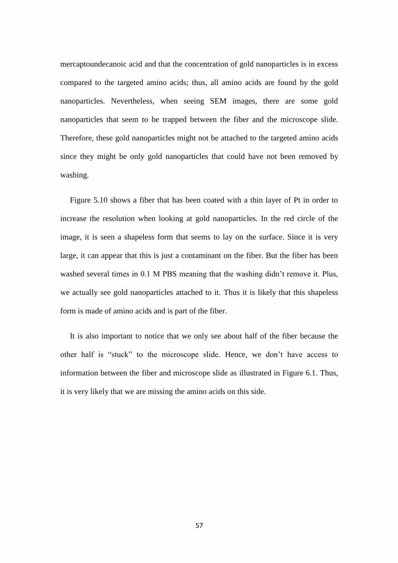
57

mercaptoundecanoic acid and that the concentration of gold nanoparticles is in excess

compared to the targeted amino acids; thus, all amino acids are found by the gold

nanoparticles. Nevertheless, when seeing SEM images, there are some gold

nanoparticles that seem to be trapped between the fiber and the microscope slide.

Therefore, these gold nanoparticles might not be attached to the targeted amino acids

since they might be only gold nanoparticles that could have not been removed by

washing.

Figure 5.10 shows a fiber that has been coated with a thin layer of Pt in order to

increase the resolution when looking at gold nanoparticles. In the red circle of the

image, it is seen a shapeless form that seems to lay on the surface. Since it is very

large, it can appear that this is just a contaminant on the fiber. But the fiber has been

washed several times in 0.1 M PBS meaning that the washing didn’t remove it. Plus,

we actually see gold nanoparticles attached to it. Thus it is likely that this shapeless

form is made of amino acids and is part of the fiber.

It is also important to notice that we only see about half of the fiber because the

other half is “stuck” to the microscope slide. Hence, we don’t have access to

information between the fiber and microscope slide as illustrated in Figure 6.1. Thus,

it is very likely that we are missing the amino acids on this side.

58

Figure 6.1: Scheme explaining how gold nanoparticles do not appear. (a) Side look

of the spider dragline silk with functionalized gold nanoparticles attached to it. (b)

Top view of this same spider dragline silk as if using SEM, showing that gold

nanoparticles at the bottom of the fiber in (a) are missing.

Since we know that the primary structure of the dragline silk (i.e., the sequence of

amino acids) has a regular pattern in the core, it was investigated if electrically

charged amino acids also show a certain spatial frequency on the surface. From the

amino acids sequence in the core, we know that they have no spatial frequency. But

Sponner et al. [6.1] investigated the protein composition of each silk layer and they

suggested that the skin layer is not made of the two main proteins MaSp1 and MaSp2.

Hence, the core composition may differ from the surface composition and we might

see regular distribution of these amino acids.

A possible pattern can be seen on the right image of Figure 5.9 that locates the

negatively charged amino acids. It is seen in the red circle that gold nanoparticles are

spread as if doing a helix around the fiber (helix which is in fact a line because the

fiber is cylindrical). Other images coming from this same fiber also showed this type

of arrangement at different locations, but another fiber analyzed (Left image of Figure

5.9) did not show this pattern at all. Moreover, the left image of Figure 5.9 shows two

fibers next to each other and it is difficult to identify any pattern since gold

59

nanoparticles in the middle of these two fibers may just be trapped. However, these

two fibers stuck two each other are most likely dragline silks fiber because there is

two major ampullate spigots that produce the dragline silk (Figure 3.2). Images that

locate positively charged amino acids did not demonstrate any pattern, and these

amino acids are spread randomly on the surface.

In order to have a better look at the distribution of the electrically charged amino

acids, a bundle of fibers have been investigated. From Figure 5.11 and Figure 5.12 we

still see that there is more negatively charged amino acids spread on the surface

compared to the positively charged amino acids. About the pattern seen for the

negatively charged amino acids, it was not seen in the images of the bundle. The fact

that we can see two fibers stuck to each other (as seen on Figure 5.9 also), preventing

us to really see how the amino acids are spread on the surface, did not help to confirm

the existence of this pattern. Then, some clusters of gold nanoparticles have been

identified on the dragline silk surface. It is unlikely that the entire surface covered by

the cluster contain the type of amino acids we are looking at, meaning that we will

have a polypeptide chain with a long sequence of glutamic/aspartic acid. But this

cluster may hide a certain amount of these amino acids and affect the vision we have

of their distribution. Further investigations need to be done using a bundle of fiber

with distinct, separated dragline silks.

60

CHAPTER SEVEN

CONCLUSION

This study determined the surface topography of N. clavipes spider dragline silk

taken in its natural state, by the use of atomic force microscopy in 0.01 M phosphate

buffered saline. Characterization of the surface showed a structure exhibiting different

level of roughness ranging from 20 nm to 100 nm. We also observed skin surface

cracking that might have been due to the stress induced during the sample preparation

but this needs further investigation. We determined that the roughness is independent

of the collection speed, and approximate average roughness values are around 50 nm,

using a scan size area of 2 µm x 2 µm and a 2nd

order planefitting (roughness is

dependent on scan area). The change in roughness as a function of time since silk

collection was also investigated, and we found no significant change, meaning that

roughness is independent of aging time.

The second part of this thesis characterized the chemical composition of the

surface of N. clavipes dragline silk by analyzing the positively and negatively charged

amino acids present on the surface of the dragline silk. These two types of amino

acids were mapped on the surface by the application of a novel technique used by B.

Zimmerman et al. on wool fibers. The areal density of negatively charged amino

acids (glutamic acid and aspartic acid) is higher than the positively charged ones

(lysine, asparagine, and histidine). This generally agrees with the relative amounts of

amino acids found in the bulk of the silk by amino acid analysis. We noticed that the

negatively charged amino acids might be spaced regularly at some locations along the

61

fiber. However, positively charged amino acids do not show a patterned arrangement;

they appear randomly arranged on the surface.

Our investigation of the surface of N. clavipes dragline silk has provided an insight

into the difference between the core and surface composition, but additional work

needs to be done in this regard. The content of negatively and positively charged

amino acids can be estimated from SEM pictures using statistical area analysis with

MATLAB. By calculating the proportion of white pixels (corresponding to the gold

nanoparticles linked to the electrically charged amino acids) over dark pixels

(corresponding to the part of the fiber that doesn’t have the amino acid we are looking

at), we will be able to have a rough quantitative value of their content. In addition,

future work on surface morphology as a function of strain using a prescribed load will

be interesting to investigate. Using AFM, the strain at which the worm-like fracture

structures we observed can be identified and an attempt to match these strain forces

with breaking forces in proteins may be done. The surface roughness as a function of

strain can be investigated at the same time as well.

62

APPENDICES

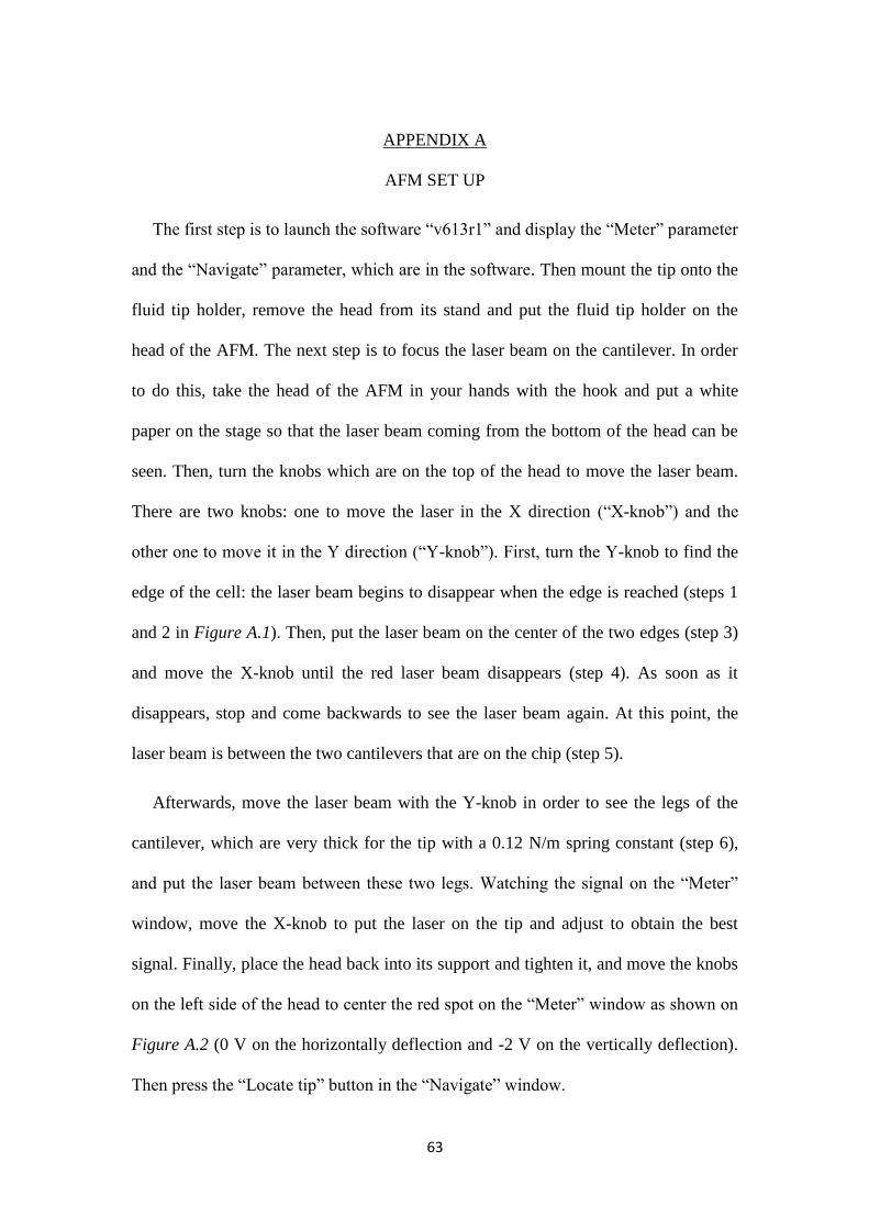
63

APPENDIX A

AFM SET UP

The first step is to launch the software “v613r1” and display the “Meter” parameter

and the “Navigate” parameter, which are in the software. Then mount the tip onto the

fluid tip holder, remove the head from its stand and put the fluid tip holder on the

head of the AFM. The next step is to focus the laser beam on the cantilever. In order

to do this, take the head of the AFM in your hands with the hook and put a white

paper on the stage so that the laser beam coming from the bottom of the head can be

seen. Then, turn the knobs which are on the top of the head to move the laser beam.

There are two knobs: one to move the laser in the X direction (“X-knob”) and the

other one to move it in the Y direction (“Y-knob”). First, turn the Y-knob to find the

edge of the cell: the laser beam begins to disappear when the edge is reached (steps 1

and 2 in Figure A.1). Then, put the laser beam on the center of the two edges (step 3)

and move the X-knob until the red laser beam disappears (step 4). As soon as it

disappears, stop and come backwards to see the laser beam again. At this point, the

laser beam is between the two cantilevers that are on the chip (step 5).

Afterwards, move the laser beam with the Y-knob in order to see the legs of the

cantilever, which are very thick for the tip with a 0.12 N/m spring constant (step 6),

and put the laser beam between these two legs. Watching the signal on the “Meter”

window, move the X-knob to put the laser on the tip and adjust to obtain the best

signal. Finally, place the head back into its support and tighten it, and move the knobs

on the left side of the head to center the red spot on the “Meter” window as shown on

Figure A.2 (0 V on the horizontally deflection and -2 V on the vertically deflection).

Then press the “Locate tip” button in the “Navigate” window.

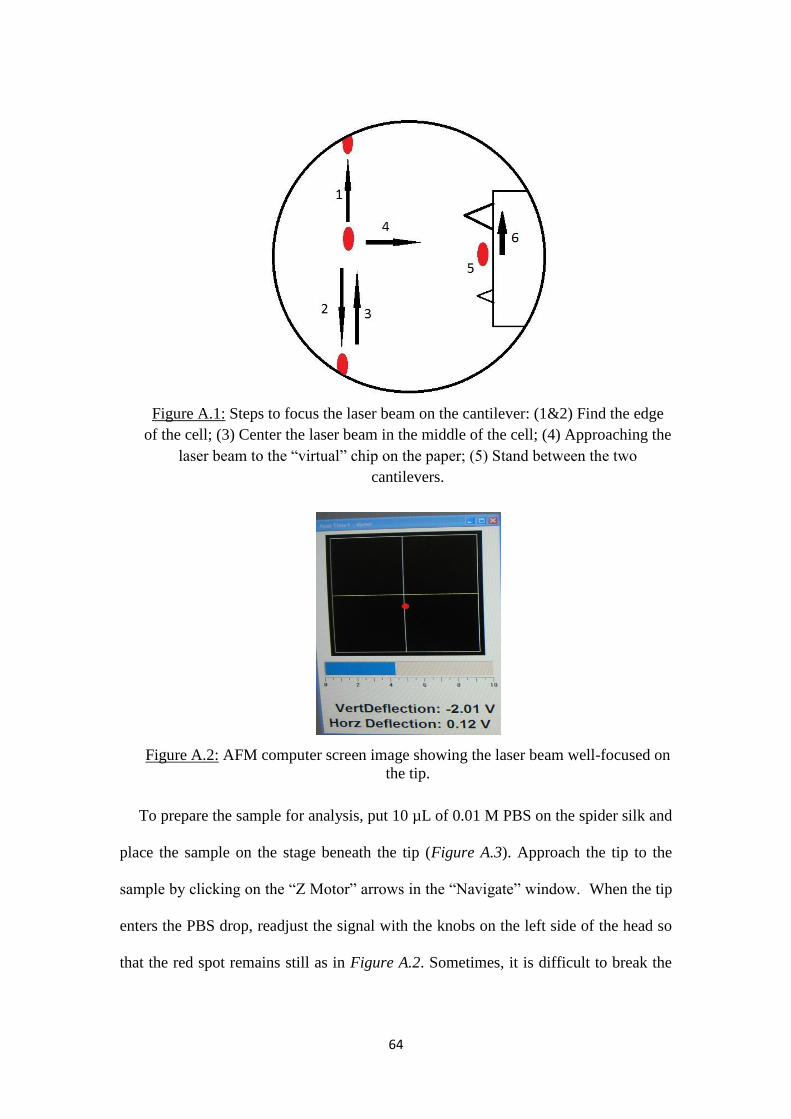
64

Figure A.1: Steps to focus the laser beam on the cantilever: (1&2) Find the edge

of the cell; (3) Center the laser beam in the middle of the cell; (4) Approaching the

laser beam to the “virtual” chip on the paper; (5) Stand between the two

cantilevers.

Figure A.2: AFM computer screen image showing the laser beam well-focused on

the tip.

To prepare the sample for analysis, put 10 µL of 0.01 M PBS on the spider silk and

place the sample on the stage beneath the tip (Figure A.3). Approach the tip to the

sample by clicking on the “Z Motor” arrows in the “Navigate” window. When the tip

enters the PBS drop, readjust the signal with the knobs on the left side of the head so

that the red spot remains still as in Figure A.2. Sometimes, it is difficult to break the

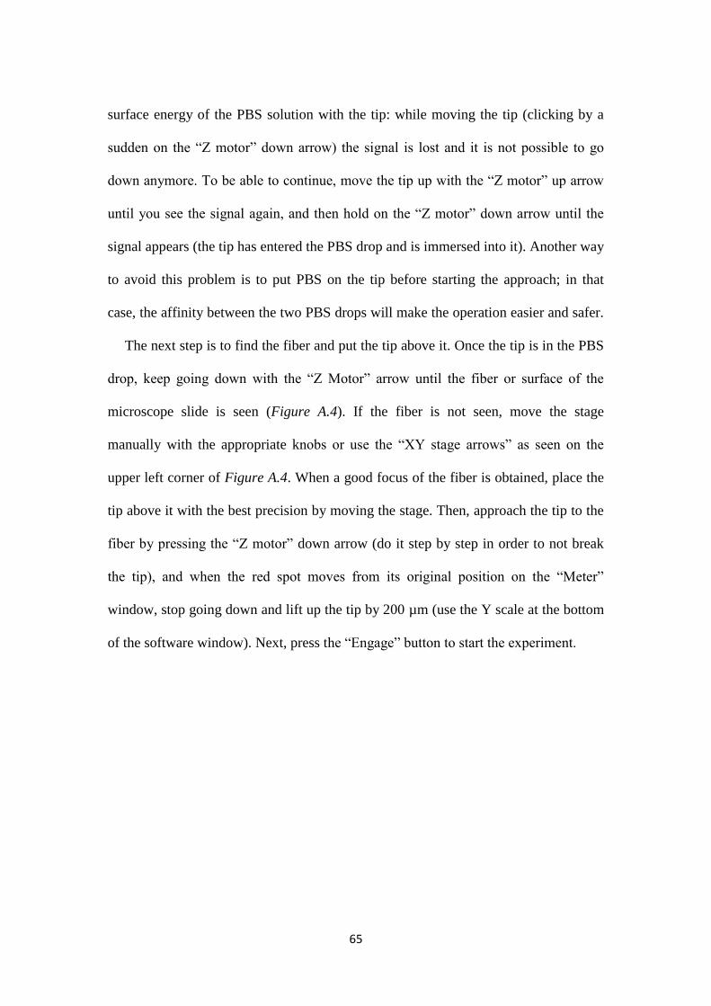
65

surface energy of the PBS solution with the tip: while moving the tip (clicking by a

sudden on the “Z motor” down arrow) the signal is lost and it is not possible to go

down anymore. To be able to continue, move the tip up with the “Z motor” up arrow

until you see the signal again, and then hold on the “Z motor” down arrow until the

signal appears (the tip has entered the PBS drop and is immersed into it). Another way

to avoid this problem is to put PBS on the tip before starting the approach; in that

case, the affinity between the two PBS drops will make the operation easier and safer.

The next step is to find the fiber and put the tip above it. Once the tip is in the PBS

drop, keep going down with the “Z Motor” arrow until the fiber or surface of the

microscope slide is seen (Figure A.4). If the fiber is not seen, move the stage

manually with the appropriate knobs or use the “XY stage arrows” as seen on the

upper left corner of Figure A.4. When a good focus of the fiber is obtained, place the

tip above it with the best precision by moving the stage. Then, approach the tip to the

fiber by pressing the “Z motor” down arrow (do it step by step in order to not break

the tip), and when the red spot moves from its original position on the “Meter”

window, stop going down and lift up the tip by 200 µm (use the Y scale at the bottom

of the software window). Next, press the “Engage” button to start the experiment.

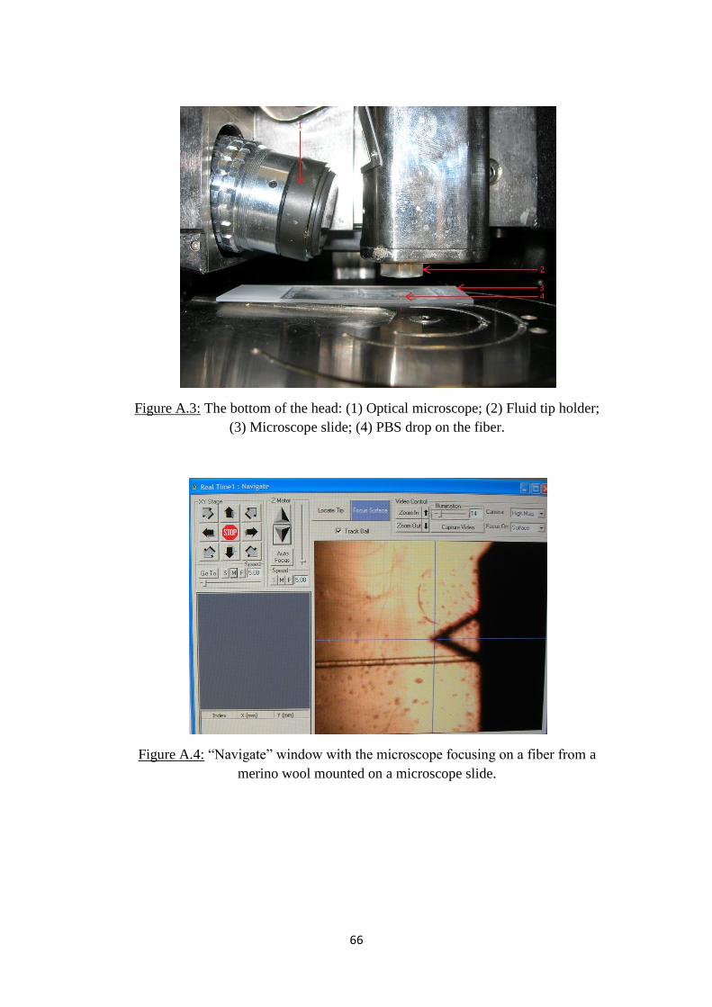
66

Figure A.3: The bottom of the head: (1) Optical microscope; (2) Fluid tip holder;

(3) Microscope slide; (4) PBS drop on the fiber.

Figure A.4: “Navigate” window with the microscope focusing on a fiber from a

merino wool mounted on a microscope slide.

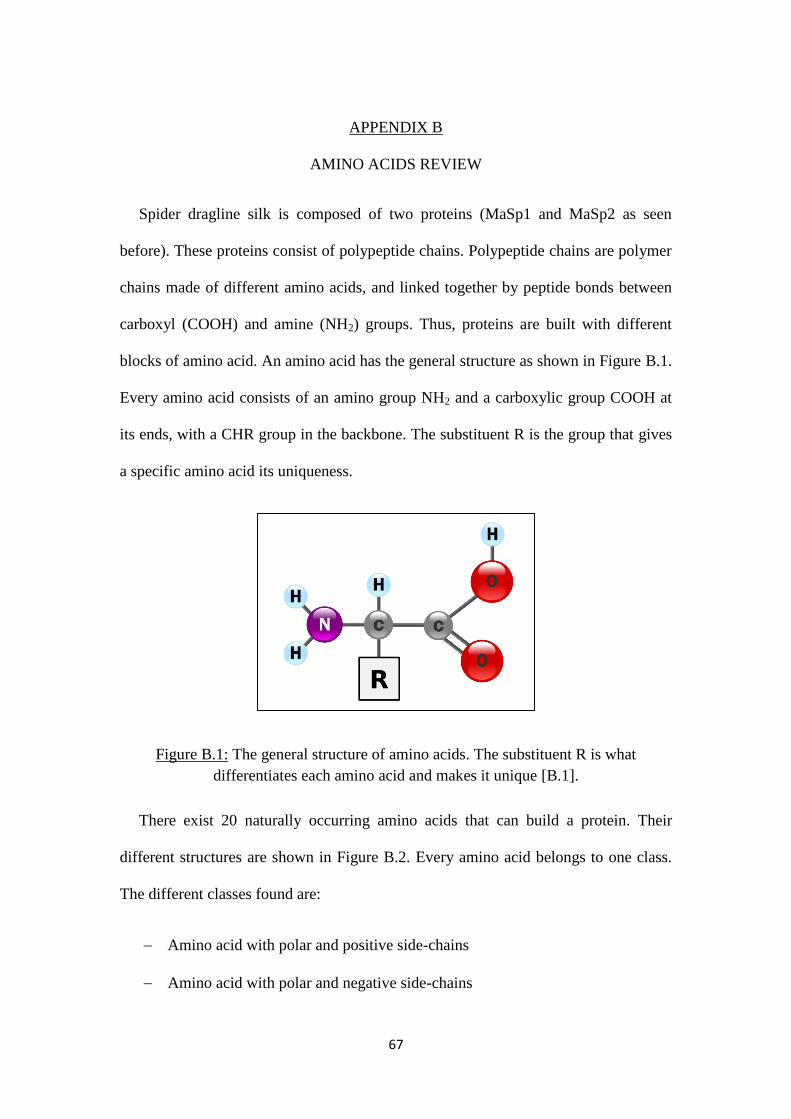
67

APPENDIX B

AMINO ACIDS REVIEW

Spider dragline silk is composed of two proteins (MaSp1 and MaSp2 as seen

before). These proteins consist of polypeptide chains. Polypeptide chains are polymer

chains made of different amino acids, and linked together by peptide bonds between

carboxyl (COOH) and amine (NH2) groups. Thus, proteins are built with different

blocks of amino acid. An amino acid has the general structure as shown in Figure B.1.

Every amino acid consists of an amino group NH2 and a carboxylic group COOH at

its ends, with a CHR group in the backbone. The substituent R is the group that gives

a specific amino acid its uniqueness.

Figure B.1: The general structure of amino acids. The substituent R is what

differentiates each amino acid and makes it unique [B.1].

There exist 20 naturally occurring amino acids that can build a protein. Their

different structures are shown in Figure B.2. Every amino acid belongs to one class.

The different classes found are:

Amino acid with polar and positive side-chains

Amino acid with polar and negative side-chains

68

Amino acid with polar and uncharged side-chains

Amino acid with nonpolar and uncharged side-chains

Figure B.2: The different amino acids and their detailed structures. They are also

separated in the group they belong to. The R group shown in Figure B.1 is highlighted

in blue or grey [B.2].

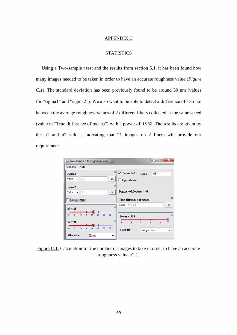
69

APPENDIX C

STATISTICS

Using a Two-sample t test and the results from section 5.1, it has been found how

many images needed to be taken in order to have an accurate roughness value (Figure

C.1). The standard deviation has been previously found to be around 30 nm (values

for “sigma1” and “sigma2”). We also want to be able to detect a difference of 35 nm

between the average roughness values of 2 different fibers collected at the same speed

(value in “True difference of means”) with a power of 0.958. The results are given by

the n1 and n2 values, indicating that 21 images on 2 fibers will provide our

requirement.

Figure C.1: Calculation for the number of images to take in order to have an accurate

roughness value [C.1]

70

APPENDIX D

ADDITIONAL IMAGES

The following images are AFM and SEM images. After taking AFM images, SEM

was used in order to have a bigger vision of the spider dragline silk surface. Then, it

was attempted to match AFM and SEM images together.

The images correspond to only one type of collection speed, i.e. 0.72 mm.s-1

. As

said in the chapter three, two fibers were mounted on a microscope slide and these

two same fibers were analyzed with AFM and SEM. As said in chapter five, AFM

results showed different structures. It will be found here 4 kinds of structure that was

seen on these two specific fibers with different roughness values, such as a very rough

surface (Figure D.1) or a moderately rough surface (Figure D.2, Figure D.3 and

Figure D.4).

Figure D.1: (Left) 3 µm x 3 µm AFM image of N. clavipes spider dragline silk

collected at 0.72mm.s-1

. In a box of 2 µm x 2 µm, the AFM image roughness is 111

nm. (Right) SEM image of the same fiber that correlates with the AFM image.

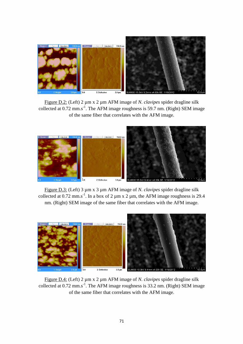
71

Figure D.2: (Left) 2 µm x 2 µm AFM image of N. clavipes spider dragline silk

collected at 0.72 mm.s-1

. The AFM image roughness is 59.7 nm. (Right) SEM image

of the same fiber that correlates with the AFM image.

Figure D.3: (Left) 3 µm x 3 µm AFM image of N. clavipes spider dragline silk

collected at 0.72 mm.s-1

. In a box of 2 µm x 2 µm, the AFM image roughness is 29.4

nm. (Right) SEM image of the same fiber that correlates with the AFM image.

Figure D.4: (Left) 2 µm x 2 µm AFM image of N. clavipes spider dragline silk

collected at 0.72 mm.s-1

. The AFM image roughness is 33.2 nm. (Right) SEM image

of the same fiber that correlates with the AFM image.

72

REFERENCES

Chapter 1

1.1 Miklosovic, D. S. Leading-edge tubercles delay stall on humpback whale

(Megaptera novaeangliae) flippers. Physics of fluids 2004, 16.

1.2 Liu, Y. Super-hydrophobic surfaces from a simple coating method: a bionic

nanoengineering aproach. Institue of Physics Publishing 2006, 17, 3259-

3263.

1.3 Qu, L. Carbon Nanotube Arrays with Strog Shear Binding-On and Easy

Normal Lifting-Off. Science 2008, 322.

1.4 J. C. Zemlin, A Study of the Mechanical Behavior of Spider's Silks. A Study

of the Mechanical Behavior of Spider's Silks 1968.

1.5 Weems, H. V.; Edwards, G. B. The Garden SIlk Fiber, Nephila Clavipes

(Linnaeus) (Arachnida: Araneae: Tetragnathidae). DPI Entomology Circular

1978.

1.6 Eisoldt, L. Decoding the secrets of spider silk. Materials today (Kidlington,

England) 2011, 14, 80-86.

1.7 Cunniff, P. Mechanical and thermal properties of dragline silk from the

spider Nephila clavipes. Polym. Adv. Technol. 1994, 5, 401-410.

1.8 Sponner, A. Composition and hierarchical organisation of a spider silk. PloS

one 2007, 2, 998.

73

1.9 Augsten, K. Glycoproteins and skin-core structure in Nephila clavipes spider

silk observed by light and electron microscopy. Scanning 2000, 22, 12-15.

1.10 Xu, M. Structure of a protein superfiber: spider dragline silk. PNAS :

Proceedings of the National Academy of Sciences 1990, 87, 7120-7124.

1.11 Hinman, M. Isolation of a clone encoding a second dragline silk fibroin.

Nephila clavipes dragline silk is a two-protein fiber. The Journal of

biological chemistry 1992, 267, 19320.

1.12 "Industrial Applications of Natural Fibres: Structure, Properties and

Technical Applications." M2 Presswire 23 July 2010.

1.13 Jelinski, L. W. Orientation, structure, wet-spinning, and molecular basis for

supercontraction of spider dragline silk. International Journal of Biological

Macromolecules 1999, 24, 197.

1.14 Warwicker, J. O., Comparative studies of fibroins: II. The crystal structures

of various fibroins. Journal of Molecular Biology 1960, 2, 350-362.

1.15 Glišović, A. Strain Dependent Structural Changes of Spider Dragline Silk.

Macromolecules 2008, 41, 390-398.

1.16 Keten, S.; Buehler, M. J. Atomistic model of the spider silk nanostructure.

Applied Physics Letters 2010, 96.

1.17 Keten, S.; Buehler, M. J. Nanostructure and molecular mechanics of spider

dragline silk protein assemblies. Journal of the Royal Society Interface 2010,

7, 1709-1721.

74

1.18 Parkhe, A. D. Structural Studies of Spider Silk Proteins in the Fiber. Journal

of Molecular Recognition 1997, 10, 1-6.

1.19 Creager, M. Solid-State NMR Comparison of Various Spiders’ Dragline Silk

Fiber. Biomacromolecules 2010, 11, 2039-2043.

1.20 Savage, K. N.; Gosline, J. M. The role of proline in the elastic mechanism of

hydrated spider silks. The Jounal of Eperimental Biology 2008, 211, 1948-

1957.

1.21 Boutry, C.; Blackledge, T. A. Evolution of supercontraction in spider silk:

structure–function relationship from tarantulas to orb-web weavers. The

journal of Experimental Biology 2010, 213, 3505-3514.

1.22 www2.dupont.com/Kevlar/en_US/assets/downloads/Oil_Gas_Brochure_08-

18-08.pdf

1.23 Gosline, J. M. The Mechanical Design of Spider Silks: From Fibroin

Sequence to Mechanical Function. The journal of Experimental Biology

1999, 202, 3295-3303.

75

REFERENCES

Chapter 2

2.1 Creager, M. Solid-State NMR Comparison of Various Spiders’ Dragline Silk

Fiber. Biomacromolecules 2010, 11, 2039-2043.

2.2 Stephen J. Lombardi, David L. Kaplan, The Amino Acid Composition of

Major Ampullate Gland Silk (Dragline) of Nephila Clavipes(Araneae,

Tetragnathidae). The Amino Acid Composition of Major Ampullate Gland

Silk (Dragline) of Nephila Clavipes(Araneae, Tetragnathidae) 1990, 18, 297.

2.3 J. C. Zemlin, A Study of the Mechanical Behavior of Spider's Silks. A Study

of the Mechanical Behavior of Spider's Silks 1968.

2.4 Van Beek J. D., The molecular structure of spider dragline silk: folding and

orientation of the protein backbone. PNAS : Proceedings of the National

Academy of Sciences 2002, 99, 10266-10271.

2.5 http://www.ipfdd.de/X-ray-Lab.197.0.html

2.6 Rousseau, M-E. Nephila clavipes spider dragline silk microstructure studied

by scanning transmission X-ray microscopy. J. Am. Chem. Soc. 2007, 129,

3897.

2.7 Glišović, A. Strain Dependent Structural Changes of Spider Dragline Silk.

Macromolecules 2008, 41, 390-398.

2.8 Grubb, D. T. Fiber Morphology of Spider Silk: The Effects of Tensile

Deformation. Macromolecules 1997, 30, 2860.

76

2.9 http://mrsec.wisc.edu/Edetc/nanoquest/afm/index.html

2.10 SPM Training Notebook, Veeco Instruments, 2003.

2.11 Li, S. F. Y. New internal structure of spider dragline silk revealed by atomic

force microscopy. Biophys. J. 1994, 66, 1209-1212.

2.12 Schäfer, A. Spider silk softening by water uptake: an AFM study. European

biophysics journal with biophysics letters 2008, 37, 197-204.

2.13 Du, N. Design of superior spider silk: From nanostructure to mechanical

properties. Biophys. J. 2006, 91, 4528-4535.

2.14 Gould, S. A. C. Short and long range order of the morphology of silk from

Latrodectus Hesperus (Black Widow) as characterized by atomic force

microscopy. International Journal of Biological Macromolecules 1999, 24,

151-157.

2.15 http://www-archive.mse.iastate.edu/microscopy/path2.html

2.16 http://www.hk-phy.org/atomic_world/tem/tem02_e.html

2.17 Sponner, A. Composition and hierarchical organisation of a spider silk. PloS

one 2007, 2, 998.

2.18 Cunniff, P. Mechanical and thermal properties of dragline silk from the

spider Nephila clavipes. Polym. Adv. Technol. 1994, 5, 401-410.

2.19 Augsten, K. Glycoproteins and skin-core structure in Nephila clavipes spider

silk observed by light and electron microscopy. Scanning 2000, 22, 12-15.

77

2.20 http://en.wikipedia.org/wiki/File:Confocalprinciple_in_English.svg

2.21 Instron Model 5848 MicroTester-Reference Manuel

2.22 Ko, F. Modeling of Mechanical Properties and Structural Design of Spider

Web. Biomacromolecules 2004, 5, 780-785.

2.23 Vollrath, F. The effect of spinning conditions on the mechanics of a spider's

dragline silk. The Royal Society 2001, 268, 2346.

78

REFERENCES

Chapter 3

3.1 SPM Training Notebook, Veeco Instruments, 2003.

3.2 Vorburger, T. V.; Raja, J. Surface Finish Metrology tutorial. NISTIR 89-

4088, 1990.

79

REFERENCES

Chapter 4

4.1 Zimmerman, B. Variation of Surface Charge along the Surface of Wool

Fibers Assessed by High-Resolution Force Spectroscopy. Journal of

Engineered Fibers and Fabrics 2011, 6.

4.2 Zimmerman, B. Mechanical and chemical Characterization of Biological

Composite Structures, MS Thesis, Clemson University, 2009.

4.3 Thermo Scientific website:

http://www.piercenet.com/browse.cfm?fldID=02040114

4.2 Sponner, A. Composition and hierarchical organisation of a spider silk. PloS

one 2007, 2, 998.

4.3 Augsten, K. Glycoproteins and skin-core structure in Nephila clavipes spider

silk observed by light and electron microscopy. Scanning 2000, 22, 12-15.

4.4 Garrett, R. H.; Grisham, C. M., Eds.; In Biochemistry; 1999

80

REFERENCES

Chapter 6

6.1 Sponner, A. Composition and hierarchical organisation of a spider silk. PloS

one 2007, 2, 998.

6.2 Augsten, K. Glycoproteins and skin-core structure in Nephila clavipes spider

silk observed by light and electron microscopy. Scanning 2000, 22, 12-15.

6.3 Zax, D. B. Variation of Mechanical Properties with Amino Acid Content in

the Silk of Nephila Clavipes. Biomacromolecules 2004, 5, 732-738.

6.4 Lynn W. Jelinski , Amy Blye, Oskar Liivak, Carl Michal, George LaVerde,

Andreas Seidel, Neeral Shah, Zhitong Yang, Orientation, structure, wet-

spinning, and molecular basis for supercontraction of spider dragline silk

1999, 24, 197.

6.5 Schäfer, A. Spider silk softening by water uptake: an AFM study. European

biophysics journal with biophysics letters 2008, 37, 197-204.

6.6 Grubb, D. T. Fiber Morphology of Spider Silk: The Effects of Tensile

Deformation. Macromolecules 1997, 30, 2860.

6.7 Savage, K. N.; Gosline, J. M. The role of proline in the elastic mechanism of

hydrated spider silks. The Jounal of Eperimental Biology 2008, 211, 1948-

1957.

81

6.8 Du, N. Design of superior spider silk: From nanostructure to mechanical

properties. Biophys. J. 2006, 91, 4528-4535.

6.9 Vollrath, F. The effect of spinning conditions on the mechanics of a spider's

dragline silk. The Royal Society 2001, 268, 2346.

6.10 Creager, M. Solid-State NMR Comparison of Various Spiders’ Dragline Silk

Fiber. Biomacromolecules 2010, 11, 2039-2043.

6.11 Stephen J. Lombardi, David L. Kaplan, The Amino Acid Composition of

Major Ampullate Gland Silk (Dragline) of Nephila Clavipes(Araneae,

Tetragnathidae). Journal of Arachnology 1990, 18, 297.

6.12 J. C. Zemlin, A Study of the Mechanical Behavior of Spider's Silks. A Study

of the Mechanical Behavior of Spider's Silks 1968.

82

REFERENCES

Appendix B

B.1 http://en.wikipedia.org/wiki/File:AminoAcidball.svg

B.2

htttp://www.personal.psu.edu/staff/m/b/mbt102/bisci4online/chemistry/chem

istry8.htm

83

REFERENCES

Appendix C

C.1 Lenth, R. V. (2001), ``Some Practical Guidelines for Effective Sample Size

Determination,'' The American Statistician, 55, 187-193.