Sparse Time-Frequency Representation in 2 Dimensions

Eric ZhangMentor: Prof. Tom Hou

May 8, 2013

1 Abstract

The analysis of data is essential to advancing science. Every day, new observations andmeasurements are made that need careful manipulation to reveal patterns and relationships.Data are also becoming integral to the rest of society, as technology becomes increasinglyinvolved in the planning, running, and study of business and ordinary life. Most current dataanalysis methods make assumptions on the data such as linearity, stationarity, or periodicity.Real life data often does not satisfy these assumptions. For this reason, more adaptive androbust methods are needed. Sparse Time-Frequency Representation (STFR) is a method ofextracting frequency and trend information from signal data. It uses the observation thatsignals are often complicated in time but can be represented compactly in the frequencydomain. Instead of having a set basis, as in Fourier Analysis, SFTR uses a large andhighly redundant dictionary. It then searches for the sparsest representation of the signal inthis dictionary. Currently, the 1 dimensional version of this method has been successfullyimplemented. Generalizing to 2 dimensions, however, presents some difficulties. Whereas1D only requires fitting in one direction, 2D must update in two directions. We are currentlyexploring methods to overcome this problem.

2 Background

STFR, or Sparse Time-Frequency Representation [5], is a recently conceived mathematicalframework for analyzing non-stationary and non-linear signals.By sampling a signal at dis-crete points in time/space and finding a basis for which the signal can be represented assparsely as possible, STFR can represent a signal f as a sum of Intrinsic Mode Functions(IMFs). Specifically, we define a dictionary as the following [3]:

D = {a(t) cos θ(t) : θ′(t) ≥ 0, a(t) ∈ V (θ)},

1

where V (θ) is a linear space consisting of functions smoother than cos θ(t):

V (θ) = span(cos(λiθ), sin(λiθ), i = 1, ..., n, λi ∈ (0, 1/2])

Every element of the dictionary D is an IMF. We then decompose the signal over thisdictionary by looking for the sparsest decomposition. The sparsest decomposition can beobtained by solving a non-linear non-convex optimization problem:

P: Minimize MSubject to:

f(t) =∑M

k=1 ak(t) cos θk(t),ak(t) cos θk(t) ∈ D, k = 1, · · · ,M

However, since this problem is NP-hard, it was conceived that an alternative formulationmight provide an approximate solution. This formulation uses the idea of Matching Pursuit.First, we look for the IMF that best fits the signal in the least-squares norm:

P2: Minimize ‖f(t)− a(t) cos θ(t)‖Subject to a(t) cos θ(t) ∈ D

Once found, it gives us the first IMF that composes f . We can then apply the samemethod to the residual, r1 = f − a(t) cos θ, to extract subsequent IMFs. The process stopsonce the residual rk is found to satisfy some specified stopping criterion

Finally, in order to solve the least-squares problem, which is non-convex, we implemented aNewton-type iterative algorithm that uses an initial guess for θ to find the envelope functiona(t) and then update θ.

3 Methods

The problems discussed in the background section have been implemented in Matlab. Thissection will discuss the specifics of the numerical algorithms.

3.1 The 1D Algorithm

1. Sample the signal f over equally spaced discrete times ti, i = 1, ..., N on [0, 1]

2. Construct the dictionary D as matrix M

3. Assume θ0 is given, n = 1

4. Solve the problem

2

P3: Minimize ‖f − bn(t) cos θn − cn(t) sin θn‖Subject to: bn(t), cn(t) ∈ V (θn)

5. The envelope is given by an(t) =√bn(t)2 + cn(t)2 and the change in theta is dθn =

arctan(− cn(t)bn(t)

)

6. Update θ: θn+1 = θn − dθn or θ′n+1 = θ′n − dθ′n7. If ‖dθn‖ > ε, where ε is some given tolerance, increment n by 1 and repeat the previous

two steps

8. Otherwise, the extracted IMF is an(t) cos θn(t)

3.2 Constructing the Dictionary V (θ)

As per (2.2), V (θ) = span(cos(λiθ), sin(λiθ), i = 1, ..., n), λi ∈ [1/15, 1/2]The space V (θ) can be encoded into a matrix by taking each basis element ei of the space,and stacking its values at the discrete times into a vector. For example, the matrix repre-senting the set cos(λ1θ), cos(λ2θ), ... cos(λmθ) is

A =

∣∣∣∣∣∣∣cos(λ1θ(t1)) cos(λ2θ(t1)) · · · cos(λmθ(t1))

.... . . . . .

...cos(λ1θ(tn)) cos(λ2θ(tn)) · · · cos(λmθ(tn))

∣∣∣∣∣∣∣3.3 Solving the L1-Least Squares Problem

Step 4 of the algorithm in 3.1 is not guaranteed to converge if we just optimize over a 2-norm. This is because the dictionary is highly redundant. To fix this, a 1-norm is added tothe problem to make it numerically stable and also sparse. We use the Interior Point Codedeveloped in Matlab by Boyd, Koh, and Kim in Matlab [1] for solving the problem

Minimize ‖x‖1 + δ‖Ax− y‖L2

where the user specifies the matrix A and the tradeoff factor δ. In practice, we requirethat δ > 0 so that the problem is convex. The optimal choice of δ to use in our algorithm iscurrently unknown to us. In practice, we used a value of 0.1. Also, we used tolerance levelsof 10−5 or 10−6 for the numerical convergence of the regularized problem.

3.4 2D Attempts

3.4.1 First Attempt - Extension of 1D Code

Given the successful application of the algorithm for 1-dimensional signals (see Diane Guig-nard’s report [2]), it was believed that a simple extension might be applied to 2-dimensional

3

signals as follows:

Given the discretized grid of nodes

G =

∣∣∣∣∣∣∣(x1, y1) (x2, y1) · · · (xn, y1)

.... . . . . .

...(x1, ym) (x2, ym) · · · (xn, ym)

∣∣∣∣∣∣∣we can construct the vector of points∣∣(x1, y1) (x2, y1) · · · (xn, y1) (x1, y2) (x2, y2) · · · (xn, ym)

∣∣Tby stacking columns of G on top of each other into a vector form. We can then apply the 1Dalgorithm, treating each node in the vector as if it represented a discrete time. The resultsare mixed - if the initial guess for θ is good (the direction of propagation is the same as thatof the real θ), the extraction is accurate. Otherwise, the algorithm gives inaccurate results.

3.4.2 Intermediate Attempts

These following algorithms were attempts to solve the issue of the directionality of updatingthat was encountered in the initial attack of the 2D problem.

Algorithm 1

In this algorithm, V (θ) is composed of linear combinations of sinusoids such as cos(λiθ), cos(λiψ),where ψ is the approximate harmonic conjugate of θ, as computed with Kirill Pankratov’sstreamfunction program [4]. It was believed at the time that expanding the dictionary thisway would solve the problem of sensitivity to the initial guess for θ. By computing the (ap-proximate) harmonic conjugate, we found a function whose gradient would be orthogonal orat least linearly independent of θ at every point. In theory, this would allow the algorithmto better update the gradient of θ by

1. Start with 2-dimensional signal f(x, y), initial guess θ(x, y), n = 0

2. While ‖dθ‖ < tol AND iter < max

Using θn, construct harmonic conjugate ψn

Using θn and ψn, construct dictionary D

Extract the envelope function:

minimizean∈D

‖an‖1 + ‖f − an cos θn‖L2

4

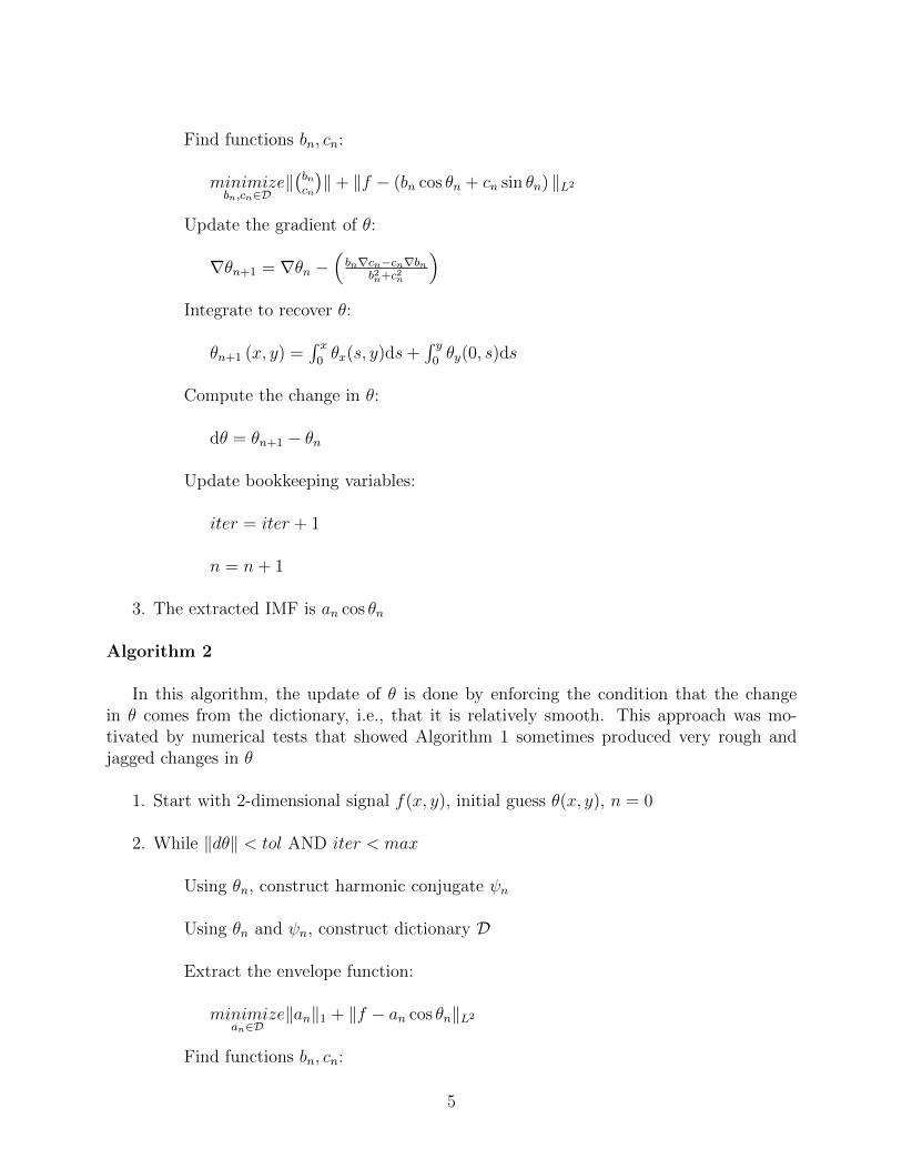
Find functions bn, cn:

minimizebn,cn∈D

‖(bncn

)‖+ ‖f − (bn cos θn + cn sin θn) ‖L2

Update the gradient of θ:

∇θn+1 = ∇θn −(bn∇cn−cn∇bn

b2n+c2n

)Integrate to recover θ:

θn+1 (x, y) =∫ x

0θx(s, y)ds+

∫ y0θy(0, s)ds

Compute the change in θ:

dθ = θn+1 − θn

Update bookkeeping variables:

iter = iter + 1

n = n+ 1

3. The extracted IMF is an cos θn

Algorithm 2

In this algorithm, the update of θ is done by enforcing the condition that the changein θ comes from the dictionary, i.e., that it is relatively smooth. This approach was mo-tivated by numerical tests that showed Algorithm 1 sometimes produced very rough andjagged changes in θ

1. Start with 2-dimensional signal f(x, y), initial guess θ(x, y), n = 0

2. While ‖dθ‖ < tol AND iter < max

Using θn, construct harmonic conjugate ψn

Using θn and ψn, construct dictionary D

Extract the envelope function:

minimizean∈D

‖an‖1 + ‖f − an cos θn‖L2

Find functions bn, cn:

5

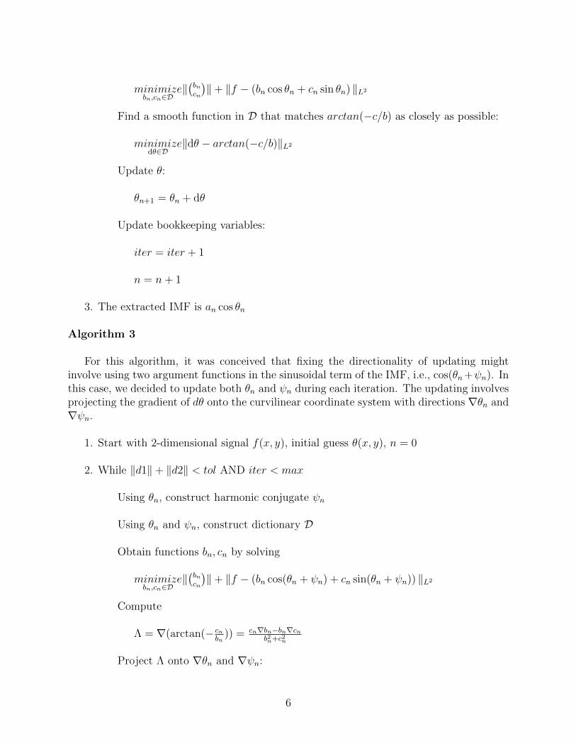
minimizebn,cn∈D

‖(bncn

)‖+ ‖f − (bn cos θn + cn sin θn) ‖L2

Find a smooth function in D that matches arctan(−c/b) as closely as possible:

minimizedθ∈D

‖dθ − arctan(−c/b)‖L2

Update θ:

θn+1 = θn + dθ

Update bookkeeping variables:

iter = iter + 1

n = n+ 1

3. The extracted IMF is an cos θn

Algorithm 3

For this algorithm, it was conceived that fixing the directionality of updating mightinvolve using two argument functions in the sinusoidal term of the IMF, i.e., cos(θn+ψn). Inthis case, we decided to update both θn and ψn during each iteration. The updating involvesprojecting the gradient of dθ onto the curvilinear coordinate system with directions ∇θn and∇ψn.

1. Start with 2-dimensional signal f(x, y), initial guess θ(x, y), n = 0

2. While ‖d1‖+ ‖d2‖ < tol AND iter < max

Using θn, construct harmonic conjugate ψn

Using θn and ψn, construct dictionary D

Obtain functions bn, cn by solving

minimizebn,cn∈D

‖(bncn

)‖+ ‖f − (bn cos(θn + ψn) + cn sin(θn + ψn)) ‖L2

Compute

Λ = ∇(arctan(− cnbn

)) = cn∇bn−bn∇cnb2n+c2n

Project Λ onto ∇θn and ∇ψn:

6

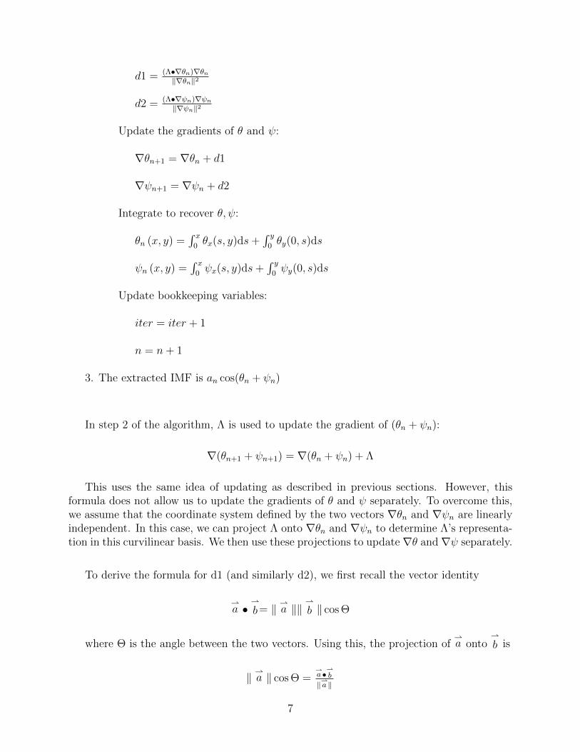
d1 = (Λ•∇θn)∇θn‖∇θn‖2

d2 = (Λ•∇ψn)∇ψn

‖∇ψn‖2

Update the gradients of θ and ψ:

∇θn+1 = ∇θn + d1

∇ψn+1 = ∇ψn + d2

Integrate to recover θ, ψ:

θn (x, y) =∫ x

0θx(s, y)ds+

∫ y0θy(0, s)ds

ψn (x, y) =∫ x

0ψx(s, y)ds+

∫ y0ψy(0, s)ds

Update bookkeeping variables:

iter = iter + 1

n = n+ 1

3. The extracted IMF is an cos(θn + ψn)

In step 2 of the algorithm, Λ is used to update the gradient of (θn + ψn):

∇(θn+1 + ψn+1) = ∇(θn + ψn) + Λ

This uses the same idea of updating as described in previous sections. However, thisformula does not allow us to update the gradients of θ and ψ separately. To overcome this,we assume that the coordinate system defined by the two vectors ∇θn and ∇ψn are linearlyindependent. In this case, we can project Λ onto ∇θn and ∇ψn to determine Λ’s representa-tion in this curvilinear basis. We then use these projections to update∇θ and∇ψ separately.

To derive the formula for d1 (and similarly d2), we first recall the vector identity

⇀a •

⇀

b= ‖ ⇀a ‖‖⇀

b ‖ cos Θ

where Θ is the angle between the two vectors. Using this, the projection of⇀a onto

⇀

b is

‖ ⇀a ‖ cos Θ =⇀a •

⇀b

‖⇀a ‖

7

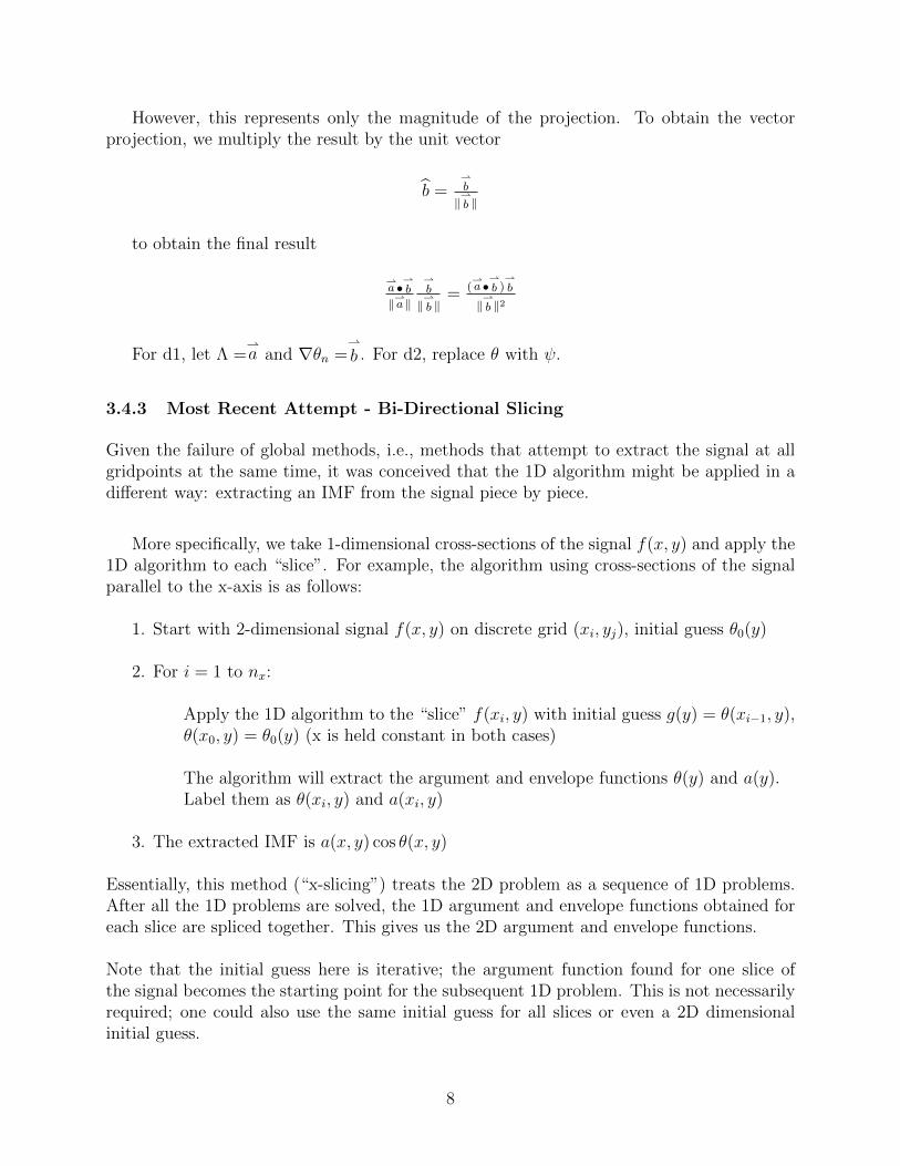
However, this represents only the magnitude of the projection. To obtain the vectorprojection, we multiply the result by the unit vector

b̂ =⇀b

‖⇀b ‖

to obtain the final result

⇀a •

⇀b

‖⇀a ‖

⇀b

‖⇀b ‖

= (⇀a •

⇀b )

⇀b

‖⇀b ‖2

For d1, let Λ =⇀a and ∇θn =

⇀

b . For d2, replace θ with ψ.

3.4.3 Most Recent Attempt - Bi-Directional Slicing

Given the failure of global methods, i.e., methods that attempt to extract the signal at allgridpoints at the same time, it was conceived that the 1D algorithm might be applied in adifferent way: extracting an IMF from the signal piece by piece.

More specifically, we take 1-dimensional cross-sections of the signal f(x, y) and apply the1D algorithm to each “slice”. For example, the algorithm using cross-sections of the signalparallel to the x-axis is as follows:

1. Start with 2-dimensional signal f(x, y) on discrete grid (xi, yj), initial guess θ0(y)

2. For i = 1 to nx:

Apply the 1D algorithm to the “slice” f(xi, y) with initial guess g(y) = θ(xi−1, y),θ(x0, y) = θ0(y) (x is held constant in both cases)

The algorithm will extract the argument and envelope functions θ(y) and a(y).Label them as θ(xi, y) and a(xi, y)

3. The extracted IMF is a(x, y) cos θ(x, y)

Essentially, this method (“x-slicing”) treats the 2D problem as a sequence of 1D problems.After all the 1D problems are solved, the 1D argument and envelope functions obtained foreach slice are spliced together. This gives us the 2D argument and envelope functions.

Note that the initial guess here is iterative; the argument function found for one slice ofthe signal becomes the starting point for the subsequent 1D problem. This is not necessarilyrequired; one could also use the same initial guess for all slices or even a 2D dimensionalinitial guess.

8

Finally, note that since the 1D algorithm gives errors on the boundaries, “x-slicing” mayproduce errors when x = x1 or xnx (first and last cross-sections). However, these same errorsare not produced when “y-slicing,” that is, when we apply the 1D algorithm to cross-sectionsof the signal where y is constant. On the other hand, y-slicing may give, due to the sameproblem with boundary errors, inaccurate results when y = y1 or yny . Consequently, it isadvantageous to apply “slicing” in both the x and y directions and then use the results of onedirection to compensate for errors with the direction. In my numerical experiments, I choseto average the two directions with equal weights. Although more sophisticated combinationsare possible, I found that simple averaging was sufficient to reduce errors on the boundary.

4 Results of Algorithms

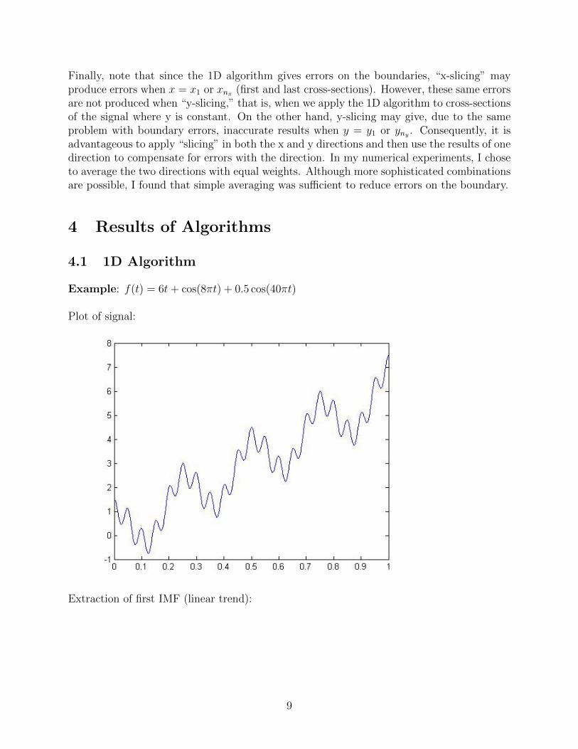
4.1 1D Algorithm

Example: f(t) = 6t+ cos(8πt) + 0.5 cos(40πt)

Plot of signal:

Extraction of first IMF (linear trend):

9

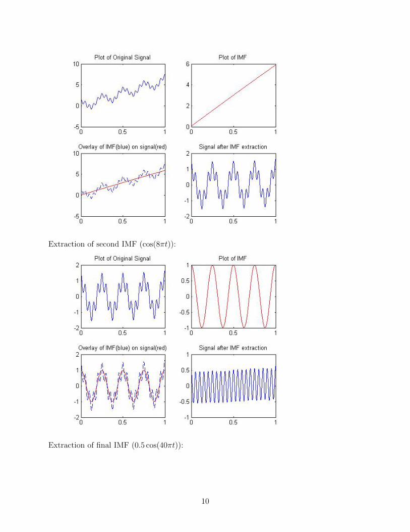
Extraction of second IMF (cos(8πt)):

Extraction of final IMF (0.5 cos(40πt)):

10

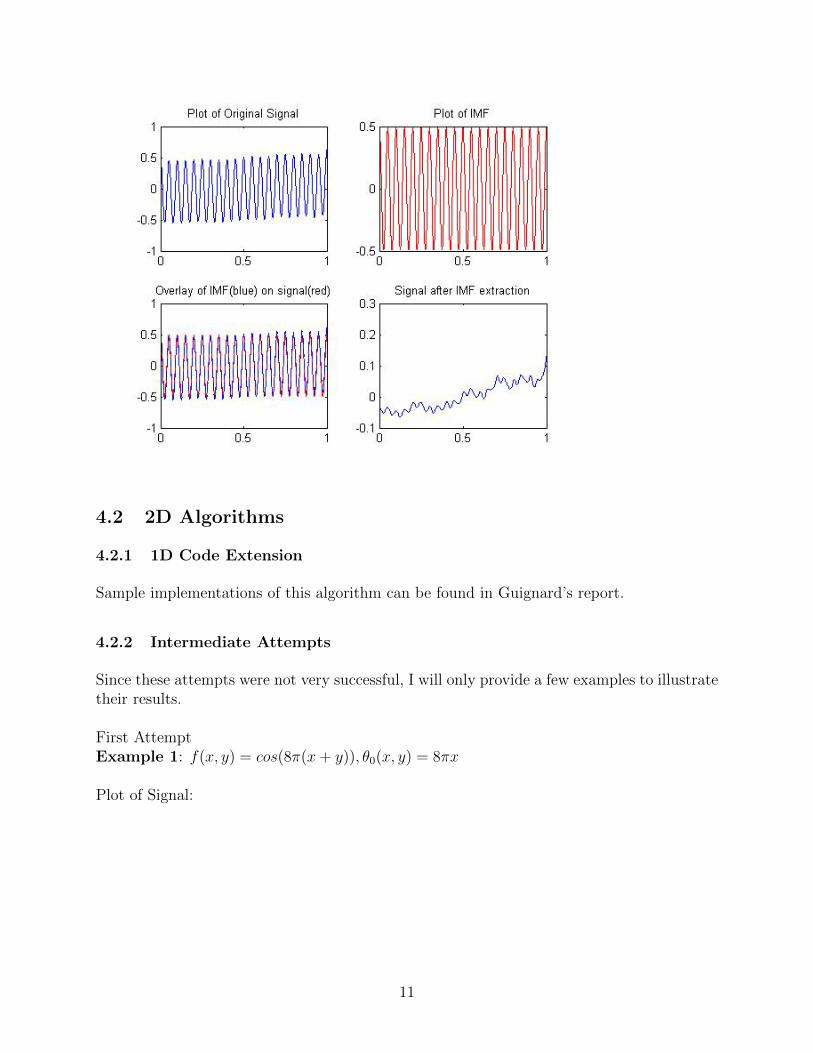
4.2 2D Algorithms

4.2.1 1D Code Extension

Sample implementations of this algorithm can be found in Guignard’s report.

4.2.2 Intermediate Attempts

Since these attempts were not very successful, I will only provide a few examples to illustratetheir results.

First AttemptExample 1: f(x, y) = cos(8π(x+ y)), θ0(x, y) = 8πx

Plot of Signal:

11

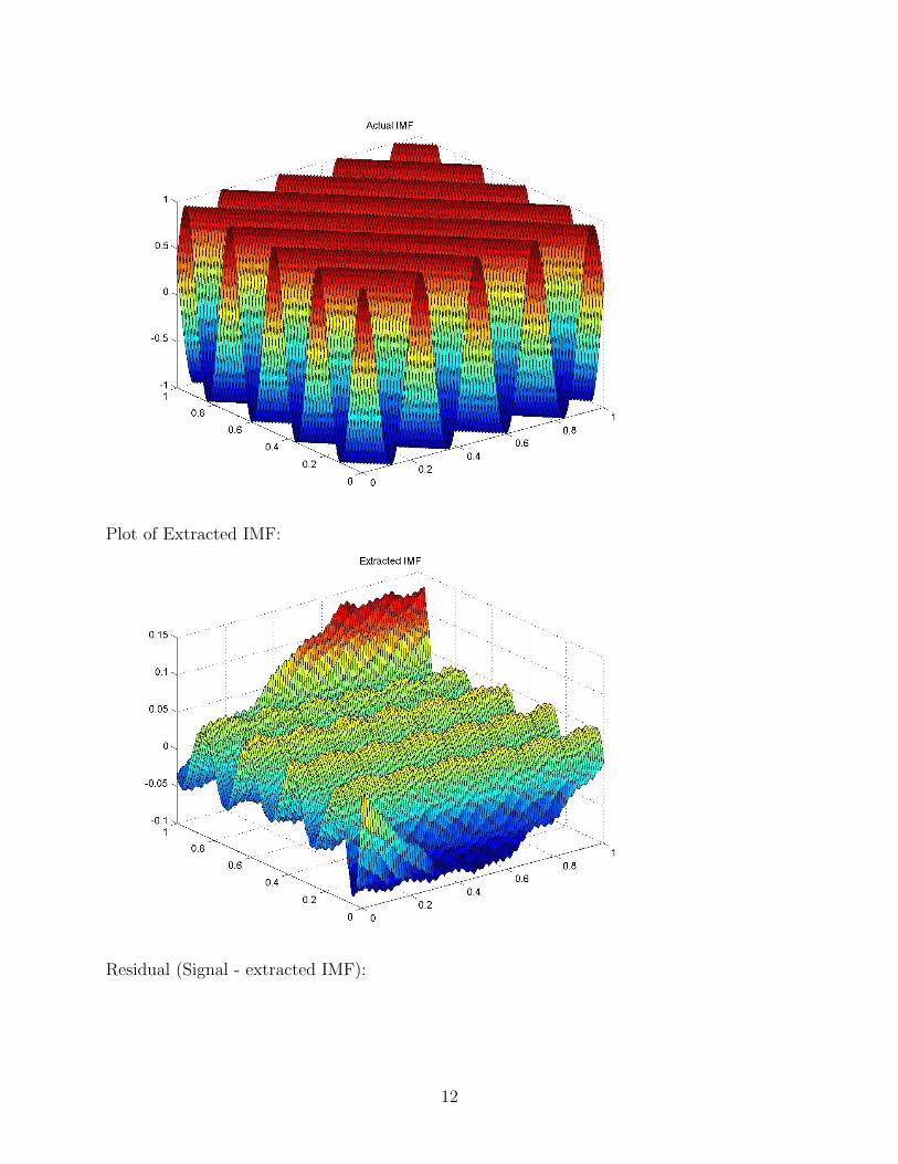
Plot of Extracted IMF:

Residual (Signal - extracted IMF):

12

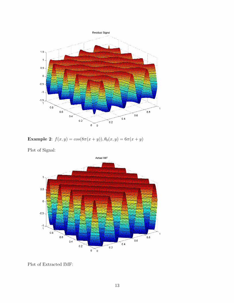
Example 2: f(x, y) = cos(8π(x+ y)), θ0(x, y) = 6π(x+ y)

Plot of Signal:

Plot of Extracted IMF:

13

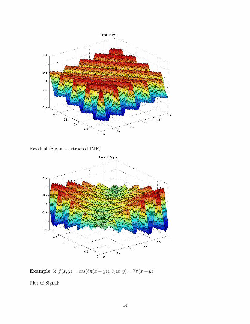
Residual (Signal - extracted IMF):

Example 3: f(x, y) = cos(8π(x+ y)), θ0(x, y) = 7π(x+ y)

Plot of Signal:

14

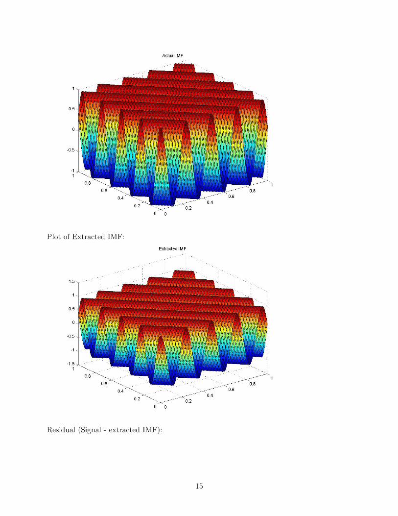
Plot of Extracted IMF:

Residual (Signal - extracted IMF):

15

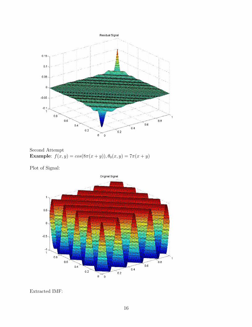
Second AttemptExample: f(x, y) = cos(8π(x+ y)), θ0(x, y) = 7π(x+ y)

Plot of Signal:

Extracted IMF:

16

Residual (Signal - extracted IMF):

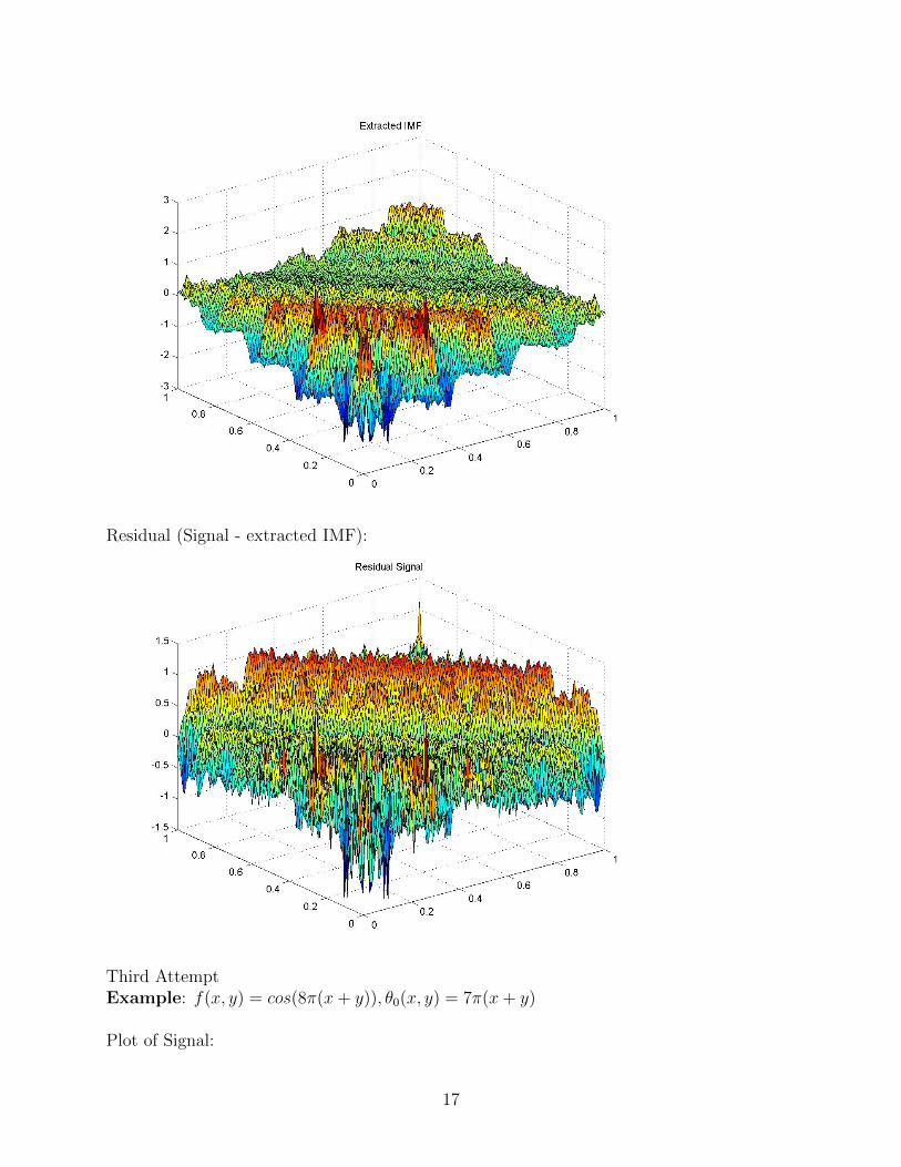
Third AttemptExample: f(x, y) = cos(8π(x+ y)), θ0(x, y) = 7π(x+ y)

Plot of Signal:

17

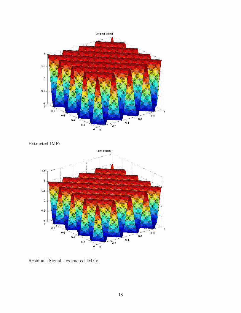
Extracted IMF:

Residual (Signal - extracted IMF):

18

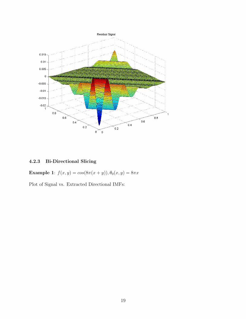
4.2.3 Bi-Directional Slicing

Example 1: f(x, y) = cos(8π(x+ y)), θ0(x, y) = 8πx

Plot of Signal vs. Extracted Directional IMFs:

19

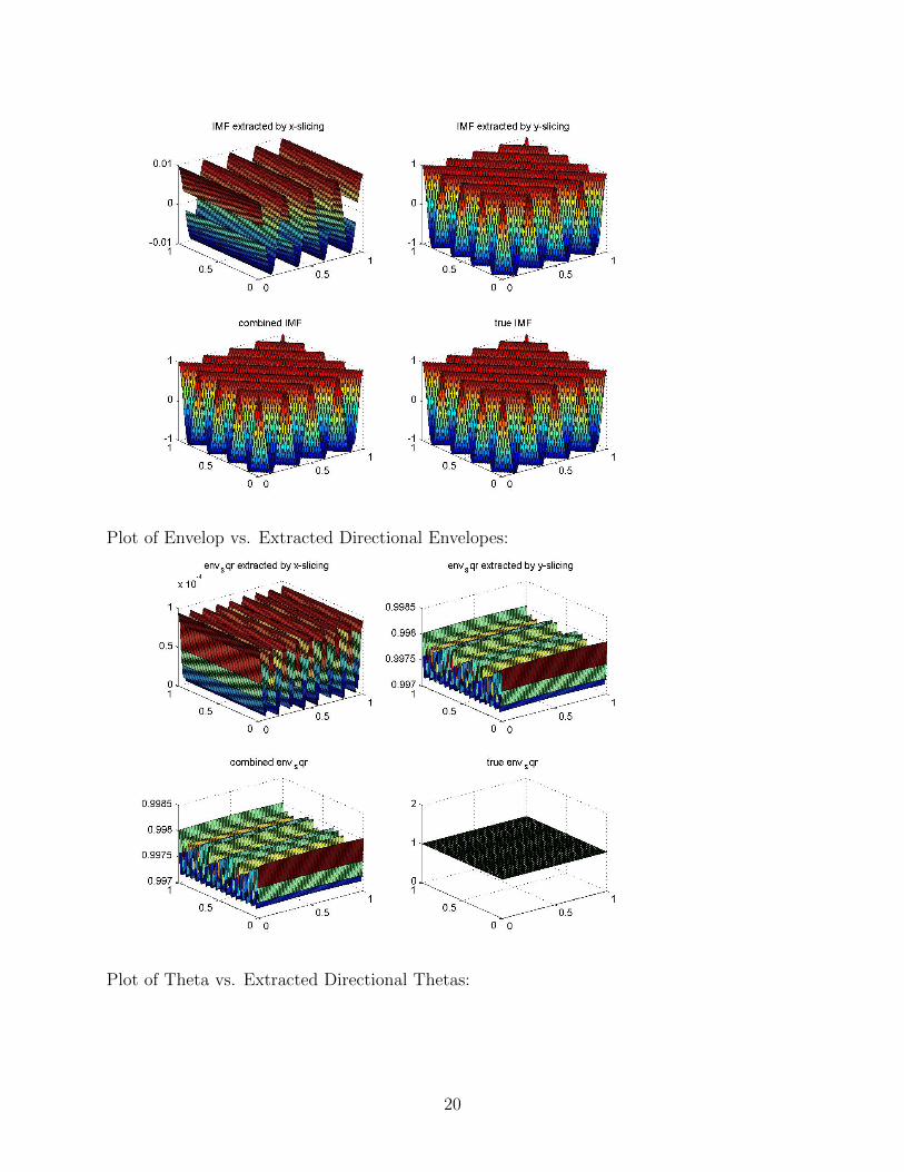
Plot of Envelop vs. Extracted Directional Envelopes:

Plot of Theta vs. Extracted Directional Thetas:

20

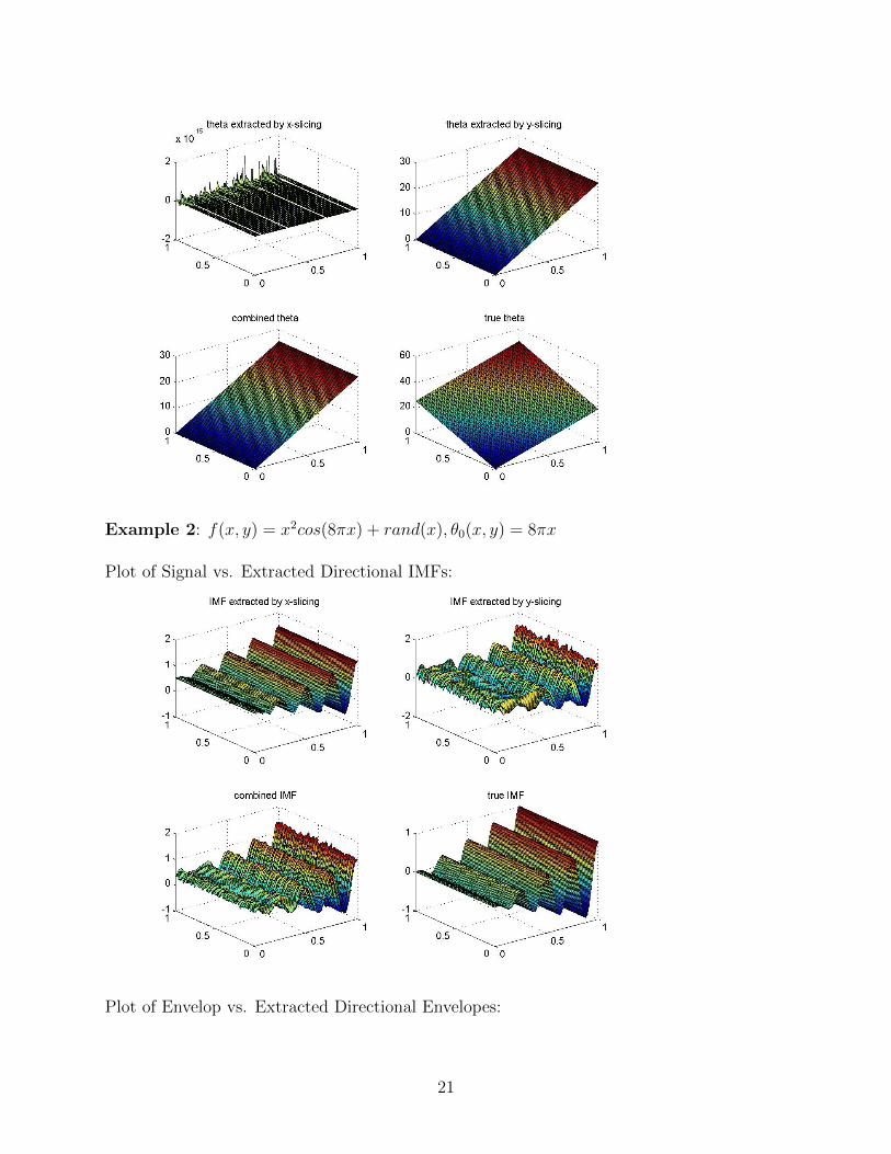
Example 2: f(x, y) = x2cos(8πx) + rand(x), θ0(x, y) = 8πx

Plot of Signal vs. Extracted Directional IMFs:

Plot of Envelop vs. Extracted Directional Envelopes:

21

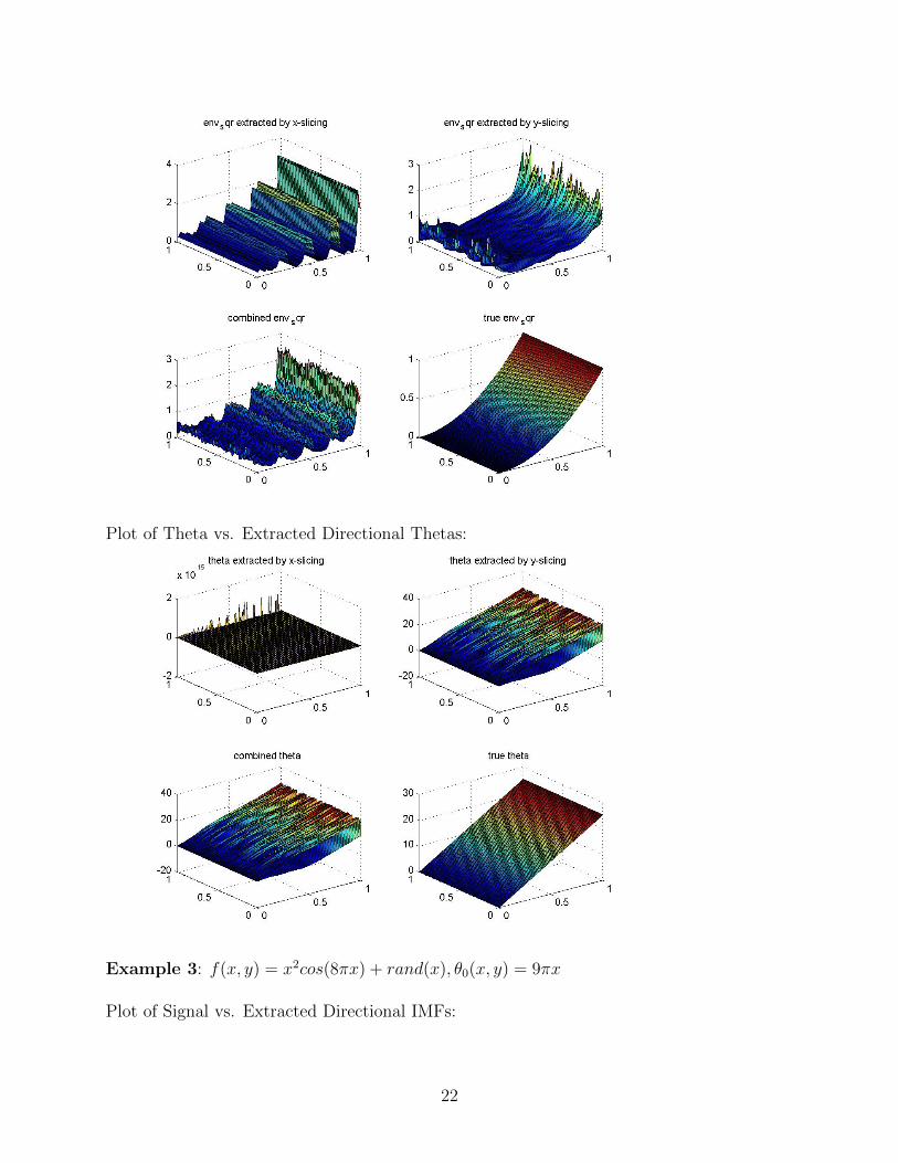
Plot of Theta vs. Extracted Directional Thetas:

Example 3: f(x, y) = x2cos(8πx) + rand(x), θ0(x, y) = 9πx

Plot of Signal vs. Extracted Directional IMFs:

22

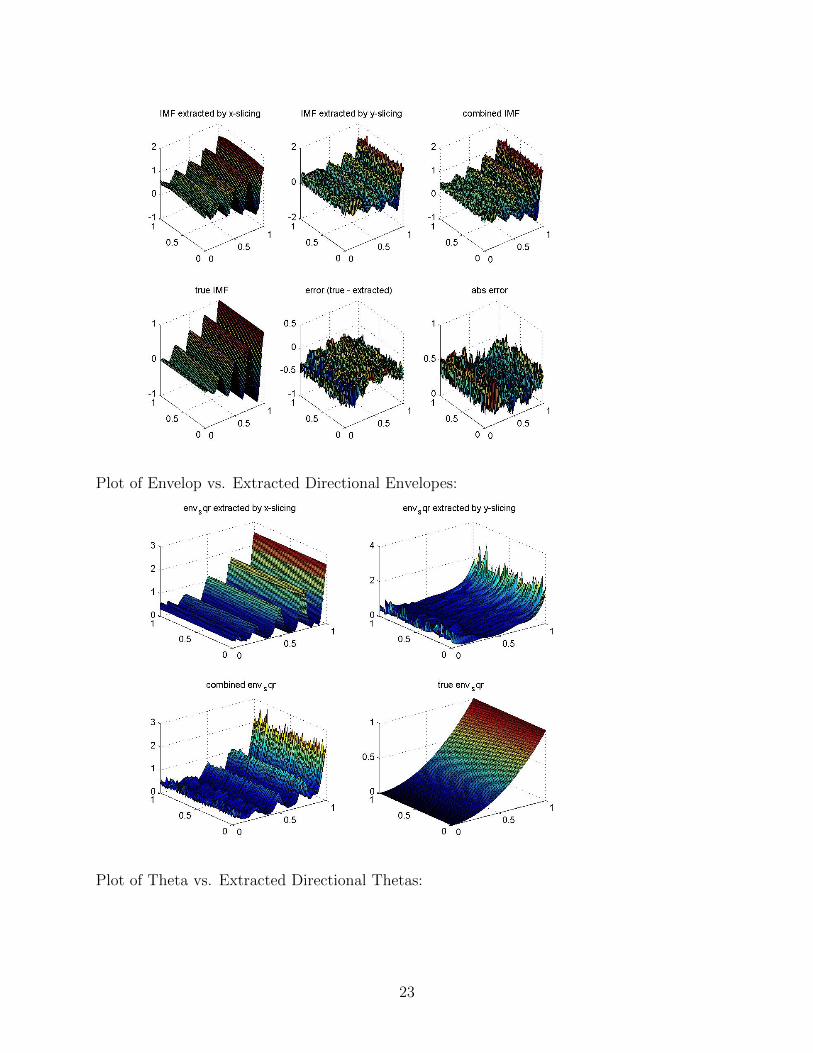
Plot of Envelop vs. Extracted Directional Envelopes:

Plot of Theta vs. Extracted Directional Thetas:

23

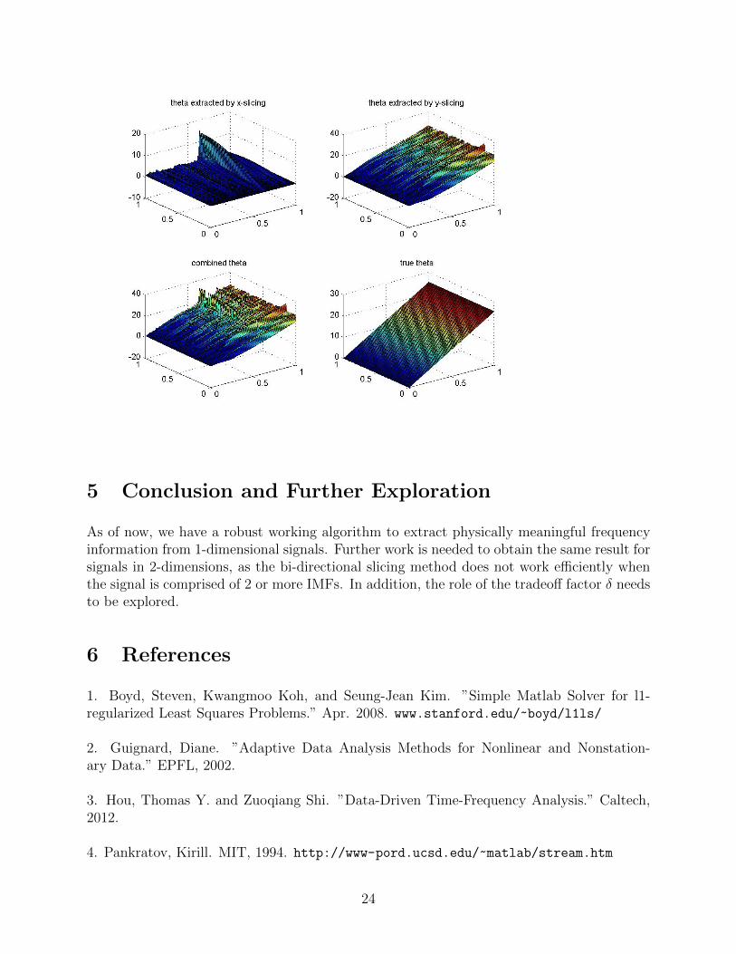
5 Conclusion and Further Exploration

As of now, we have a robust working algorithm to extract physically meaningful frequencyinformation from 1-dimensional signals. Further work is needed to obtain the same result forsignals in 2-dimensions, as the bi-directional slicing method does not work efficiently whenthe signal is comprised of 2 or more IMFs. In addition, the role of the tradeoff factor δ needsto be explored.

6 References

1. Boyd, Steven, Kwangmoo Koh, and Seung-Jean Kim. ”Simple Matlab Solver for l1-regularized Least Squares Problems.” Apr. 2008. www.stanford.edu/~boyd/l1ls/

2. Guignard, Diane. ”Adaptive Data Analysis Methods for Nonlinear and Nonstation-ary Data.” EPFL, 2002.

3. Hou, Thomas Y. and Zuoqiang Shi. ”Data-Driven Time-Frequency Analysis.” Caltech,2012.

4. Pankratov, Kirill. MIT, 1994. http://www-pord.ucsd.edu/~matlab/stream.htm

24

5. Tavallali, Peyman. ”Sparse Time Frequency Representation (STFR) and Its Applica-tions.” Caltech, 2012.

25