Suresh Ra jgopal - cs.unc.edu
201
Transcript of Suresh Ra jgopal - cs.unc.edu

c�����Suresh Rajgopal
All Rights Reserved
ii

SURESH RAJGOPAL� Spatial Entropy � A Uni�ed Attribute to ModelDynamic Communication in VLSI Circuits �Under the direction of Kye S�Hedlund and Akhilesh Tyagi�
Abstract
This dissertation addresses the problem of capturing the dynamic communication in VLSI circuits� There are several CAD problems where attributesthat combine behavior and structure are needed or when function behavior istoo complex and is best captured through some attribute in the implementation� Examples include timing analysis logic synthesis dynamic powerestimation and variable ordering for binary decision diagrams �BDDs�� Insuch a situation using static attributes computed from the structure of theimplementation is not always helpful� Firstly they do not provide su�cientusage information and secondly they tend to exhibit variances with implementations which is not desirable while capturing function behavior�The contribution of this research is a new circuit attribute called spa�
tial entropy� It models the dynamic communication e�ort in the circuit byunifying the static structure and the dynamic data usage� Quantitativelyspatial entropy measures the switching energy in a physical �CMOS� implementation� A minimumspatial entropy implementation is a minimumenergyimplementation� For the purposes of this dissertation we restrict our scopeto combinational circuits� We propose a simple procedure to estimate spatialentropy in a gate level circuit� It is characterized in extensive detail and wedescribe why it is di�cult to compute spatial entropy accurately� We showhow it can also be de�ned at other levels of abstraction�We illustrate applications of spatial entropy in BDD variable ordering
a problem that has traditionally relied on static attribute based solutions�We also show empirically that spatial entropy can track function behaviorthrough implementations by using it to measure gatecount complexity inboolean functions�
iii

Acknowledgments
I would like to take this opportunity to express my sincere gratitude towardsmy advisor Kye Hedlund and coadvisor Akhilesh Tyagi� This research wouldhave been impossible without their advice encouragement and guidance� Iwould like to thank them for the time that they have spent with me and thehours of discussions that we have had� Their comments and suggestions havegone a long way in helping me produce a comprehensive dissertation� Theyhave taught me the essence of patience in research and the need to presentideas clearly and simply� Doing research under them has been exciting andchallenging�I am indebted to my committee member Doug Reeves whose advice and
comments helped me keep this research in perspective� I gratefully acknowledge his patience encouragement and willingness to help� I would also liketo thank Don Stanat and David Plaisted for serving on my committee andfor their suggestions and encouragement� I appreciate the assistance of SujitDey �of NEC Research Labs Princeton� and Kris Kozminski of the OASISgroup at MCNC during this research�I am grateful to Yuki Watanabe for his support throughout my stay at
UNC� I would also like to thank Peter Reintjes of DASIX Intergraph for hishelp and encouragement during my graduate career and my o�ce mates atUNC Jim Symon and Don Stone for making the department a better placeto live work in�Finally I would like to thank my wife Uju for her endless patience and
support� Her strength and encouragement have been invaluable during hardtimes�
iv

Contents
� Introduction ���� Overview � � � � � � � � � � � � � � � � � � � � � � � � � � � � � ���� Motivation � � � � � � � � � � � � � � � � � � � � � � � � � � � � ���� Thesis � � � � � � � � � � � � � � � � � � � � � � � � � � � � � � � ���� Research Contributions � � � � � � � � � � � � � � � � � � � � � ���� Dissertation Outline � � � � � � � � � � � � � � � � � � � � � � � ��
� Related Work ����� Static and Dynamic Attributes � � � � � � � � � � � � � � � � � ����� Communication Complexity Prediction � � � � � � � � � � � � � ����� Entropy Based Attributes � � � � � � � � � � � � � � � � � � � � ��
����� Background � � � � � � � � � � � � � � � � � � � � � � � � ������� The Entropy function in CAD � � � � � � � � � � � � � ������� Entropy as a basis for Computation � � � � � � � � � � ��
� Spatial Entropy � A Circuit Attribute ����� Introduction and De�nitions � � � � � � � � � � � � � � � � � � � ����� Spatial Entropy Computation � � � � � � � � � � � � � � � � � � ����� Algorithm � � � � � � � � � � � � � � � � � � � � � � � � � � � � � ����� Spatial Entropy Vectors � � � � � � � � � � � � � � � � � � � � � ����� Factors a�ecting Spatial Entropy Computation � � � � � � � � ��
����� Logic Minimization and Spatial Entropy � � � � � � � � ������� Wire Length and Spatial Entropy � � � � � � � � � � � � ������� Reconvergent Fanout and Spatial Entropy � � � � � � � ��
� Spatial Entropy Based BDD Ordering ����� Introduction and Motivation � � � � � � � � � � � � � � � � � � � ��
v
����� Binary Decision Diagrams � � � � � � � � � � � � � � � � ������� The Variable Ordering Problem � � � � � � � � � � � � � ������� Motivation � � � � � � � � � � � � � � � � � � � � � � � � ��
��� Variable Ordering using Spatial Entropy � � � � � � � � � � � � ����� Experiment� Objectives and Criteria � � � � � � � � � � � � � � ��
����� Assumptions and Limitations � � � � � � � � � � � � � � ������� Data Set � � � � � � � � � � � � � � � � � � � � � � � � � � ��
��� Experiment Outline � � � � � � � � � � � � � � � � � � � � � � � ������� Software Construction and Variables Measured � � � � ��
��� Results and Observations � � � � � � � � � � � � � � � � � � � � ������� Spatial Entropy and BDD Sizes � � � � � � � � � � � � � ������� Spatial Entropy Approximations and BDD Sizes � � � ������� Spatial Entropy Vector Combination Strategies � � � � ���
��� Conclusions � � � � � � � � � � � � � � � � � � � � � � � � � � � � ���
� Spatial Entropy as a Measure of Area�Complexity ������ Motivation � � � � � � � � � � � � � � � � � � � � � � � � � � � � ������ Background � � � � � � � � � � � � � � � � � � � � � � � � � � � � ���
����� De�nitions � � � � � � � � � � � � � � � � � � � � � � � � ������ Information Content � � � � � � � � � � � � � � � � � � � � � � � ���
����� kdecomposition and Twolevel Minimization � � � � � ������ Decision Tree � � � � � � � � � � � � � � � � � � � � � � � � � � � ������ Spatial Entropy and Information Content � � � � � � � � � � � ������ Experiment � � � � � � � � � � � � � � � � � � � � � � � � � � � � ���
����� Assumptions � � � � � � � � � � � � � � � � � � � � � � � �������� Data Set � � � � � � � � � � � � � � � � � � � � � � � � � � ���
��� Experiment Outline � � � � � � � � � � � � � � � � � � � � � � � ������ Results and Observations � � � � � � � � � � � � � � � � � � � � ���
����� Results � � � � � � � � � � � � � � � � � � � � � � � � � � �������� Observations � � � � � � � � � � � � � � � � � � � � � � � ���
��� Conclusions � � � � � � � � � � � � � � � � � � � � � � � � � � � � ���
� Conclusions ����� Summary � � � � � � � � � � � � � � � � � � � � � � � � � � � � � ������ Future Research Directions � � � � � � � � � � � � � � � � � � � ���
Bibliography ��
vi

List of Tables
��� ISCAS �� Benchmark Circuit Characteristics � � � � � � � � � ����� Multilevel Circuit Characteristics from Logic Synthesis ��
Benchmarks � � � � � � � � � � � � � � � � � � � � � � � � � � � � ����� Twolevel Circuit Characteristics of Logic Synthesis �� Bench
marks � � � � � � � � � � � � � � � � � � � � � � � � � � � � � � � ����� OASIS generated Structured Circuit Characteristics � � � � � ����� Comparative BDD sizes for Logic Synthesis �� Benchmarks � ����� Comparative Statistics for Logic Synthesis �� Benchmarks � � ����� BDD sizes for Logic Synthesis �� Benchmarks relative to asyl�� ����� Comparative BDD sizes for ISCAS �� Benchmarks � � � � � � ����� Spatial entropy based ordering vs staticattribute based ap
proaches � � � � � � � � � � � � � � � � � � � � � � � � � � � � � � ������ Normalized Mean and Standard Deviation of sizes for IS
CAS�� Benchmarks � � � � � � � � � � � � � � � � � � � � � � � ������ BDD Sizes for OASISgenerated circuits � � � � � � � � � � � � ������ Mean and Standard Deviation of sizes for OASISgenerated
circuits � � � � � � � � � � � � � � � � � � � � � � � � � � � � � � � ������ Percentage improvement for OASIS circuits with wire length ������ E�ect of wire length and the SIS scripts on the Logic Synthesis
Benchmarks � � � � � � � � � � � � � � � � � � � � � � � � � � � � ������ j V j and � of sizes for Logic Synthesis �� circuits �with mini
mization and w l approximations� � � � � � � � � � � � � � � � ������ E�ect of wire length and the SIS scripts on the ISCAS ��
Benchmarks � � � � � � � � � � � � � � � � � � � � � � � � � � � � ������ Mean � Standard Deviation of sizes for ISCAS�� circuits �for
wire length and minimization approximations� � � � � � � � � ���
vii

���� Reconvergent Fanout Information for Logic Synthesis ��Benchmarks � � � � � � � � � � � � � � � � � � � � � � � � � � � � ���
���� Comparision of �S combination strategies for Logic Synthesis�� Benchmarks � � � � � � � � � � � � � � � � � � � � � � � � � � ���
���� Comparision of �S combination strategies for ISCAS �� Benchmarks � � � � � � � � � � � � � � � � � � � � � � � � � � � � � � � ���
��� �� and � input randomly generated functions � � � � � � � � � ������ �� and � input randomly generated functions � � � � � � � � � ������ Twolevel Functions from the Logic Synthesis �� Benchmarks ������ S I�f�Dk� and GC for random circuits �Set �� � � � � � � � � ������ S I�f�Dk� and GC for random circuits �Set �� � � � � � � � � ������ S I�f�Dk� and GC for random circuits �Set �� � � � � � � � � ������ Spatial Entropy and Information Content for Logic Synthesis
�� benchmarks � � � � � � � � � � � � � � � � � � � � � � � � � � ������ Mean and Variance of Spatial Entropy �S� and Information
Content �I� � � � � � � � � � � � � � � � � � � � � � � � � � � � � ������ Correlation Coe�cients for �S vs I� � � � � � � � � � � � � � � ������� Correlation Coe�cients for �GC vs I� � � � � � � � � � � � � � ������� Correlation Coe�cients for � data sets �Gate Count vs S� � � ���
viii
List of Figures
��� An Example Circuit and its Digraph Model � � � � � � � � � � ����� The Entropy Function Hw � � � � � � � � � � � � � � � � � � � ����� Spatial Entropy Computation for a Simple Circuit � � � � � � ����� Spatial Entropy Vector Computation � � � � � � � � � � � � � � ����� Example Spatial Entropy Calculation � � � � � � � � � � � � � ����� E�ect of Minimization on Spatial Entropy � � � � � � � � � � ����� A Node w with Multiple Fanouts � � � � � � � � � � � � � � � ����� Reconvergent Fanout An Example � � � � � � � � � � � � � � ����� A Circuit with a Supergate SG���� � � � � � � � � � � � � � � ������ The Supergate SG���� denoted as one Large Gate Node � � ��
��� OBDD of f � a��b� � a��b� � a��b� with orderingfa�� b�� a�� b�� a�� b�g � � � � � � � � � � � � � � � � � � � � � � � ��
��� OBDD of f with ordering fa�� a�� a�� b�� b�� b�g � � � � � � � � ����� Example Spatial Entropy Calculation � � � � � � � � � � � � � ����� Spatial Entropy Distribution for a �output function �Maxi
mum� � � � � � � � � � � � � � � � � � � � � � � � � � � � � � � � ����� Spatial Entropy Distribution for a �output function
�Weighted Multiply� � � � � � � � � � � � � � � � � � � � � � � � ����� Two implementations of the same function with di�ering Spa
tial Entropy � � � � � � � � � � � � � � � � � � � � � � � � � � � ����� The tradeo� between redundancy and wire length � � � � � � ����� Mapping of Gate Level Circuits at the Layout Level � � � � � ����� Experimental Setup � � � � � � � � � � � � � � � � � � � � � � � ������ E�ect of Minimization Scripts on the Logic Synthesis Bench
marks � � � � � � � � � � � � � � � � � � � � � � � � � � � � � � � ������ E�ect of Minimization Scripts on the ISCAS �� Benchmarks ������� E�ect of Wire Length on the Logic Synthesis Benchmarks � � ���
ix

���� E�ect of Wire Length on the ISCAS �� Benchmarks � � � � � ������� �S Combining Strategies for Logic Synthesis Benchmarks � � � ������� �S Combining Strategies for ISCAS �� Benchmarks � � � � � � ���
��� A Cube Space Representation of a � Variable Function � � � ������ Example functions of � variables a� b� c � � � � � � � � � � � � � ������ Monochromatic Cube Decomposition for �Variable Functions ������ Two di�erent Minimum Decompositions for a Function � � � � ������ Minimum �decomposition of f � ab� cd � � � � � � � � � � � ������ Decision Tree for D��f� with ordering a� b� c� d � � � � � � � � � ������ Decision Tree for D��f� with ordering a� c� b� d � � � � � � � � � ������ Implementation for f��c�a�b��abd� � � � � � � � � � � � � � � ������ Cube Space Distribution for f � ac� bc� abd � � � � � � � � ������� Implementation Constructed from Decision Tree in Figure ���� ������� Decision Tree for f � ac� bc� abd with � � c� d� a� b � � � � � ������� Decision Tree for f � ac� bc� abd with � � d� c� a� b � � � � � ������� Experiment Outline � � � � � � � � � � � � � � � � � � � � � � � ������� Regression Lines and Data plots �S vs I� � � � � � � � � � � � ������� Regression Lines and Data plots �S vs I� � � � � � � � � � � � ������� Regression Lines and Data plots �GC vs I� � � � � � � � � � � ������� Regression Lines and Data plots �GC vs I� � � � � � � � � � � ������� Regression Lines and Data plots �GC vs S� � � � � � � � � � � ������� Regression Lines and Data plots �GC vs S� � � � � � � � � � � ���
x

Chapter �
Introduction
The increasing complexity of VLSI circuit design has continually motivatedresearch in VLSI Design Automation and ComputerAidedDesign�CAD�tools for VLSI� The task of these CAD tools is to help automate and speedup the design process� Unfortunately almost all the problems that thesetools attempt to solve are NPcomplete� As a result many tools and theirunderlying algorithms can only achieve approximate solutions via heuristics�The quality of these solutions is often dictated by the information the algorithm can extract from the circuit in the form of attributes� These circuitattributes can be broadly classi�ed into static attributes and dynamic attributes� Static attributes are usually computed by examining the topologyor static structure of the circuit� For example the gate count attribute usedin logic synthesis is a static attribute� Dynamic attributes on the other handare computed by applying input data to the circuit� They capture circuit behavior or dynamic usage in contrast to static attributes that capture circuitstructure� Examples of dynamic attributes include �probability observability and controllability used in test generation algorithms� This dissertationillustrates the use of a uni�ed attribute that captures dynamic circuit usageand static circuit structure� As a physical attribute it provides a quantitativemeasure of switching energy in the circuit�Static attributes by themselves do not always provide su�cient informa
tion for algorithms to make good decisions� Since they are computed by statically examining the circuit structure they are unable to estimate how variousparts of the circuit get used over di�erent input combinations� In additionthese attributes often use information from one implementation to capture

the behavior of a function over all implementations� This overreliance onthe static structure can result in signi�cant variations in the value of theattribute over di�erent implementations� While this may seem desirable forsome purposes it is not helpful when the attribute is trying to capture aproperty of the function common to all implementations� In contrast to thisan attribute that can capture usage over all the input assignments is likelyto show less variation over di�erent implementations� This is because thisusage is common to all implementations of a function� When an attributecan combine this dynamic usage information along with the static structure�in an implementation� it can answer questions about the function and theimplementation�We have quantitatively de�ned and characterized a circuit attribute called
spatial entropy that can capture static structure and dynamic behavior in acircuit� We propose an e�cient method to compute this attribute in a givencircuit� We comprehensively analyze the attribute describe the di�cultiesin computing it the factors a�ecting its accuracy and the e�ects of variousapproximations� In CMOS circuit implementations spatial entropy yields ameasure of switching energy in the circuit by capturing the switching activity during dynamic power consumption� We illustrate its use in BDDvariable ordering a problem that has traditionally relied on static attributebased solutions� We also show that it can be used to capture function behavior through implementations by measuring of gatecount complexity inboolean functions� In this chapter we begin with an overview followed by anintroduction to the problem and the motivation behind it� Then we stateour thesis outlining its scope and assumptions� Finally major contributionsof the dissertation are outlined along with a description of the rest of thechapters�
��� Overview
VLSI circuit design is the process of transforming a highlevel behavioraldescription into mask geometry that is mapped onto silicon� Due to the complexity of the design process this task is typically performed by re�ning theinitial behavioral description over several levels of abstraction� At each levelof abstraction the circuit is described with increasing detail� This hierarchyof levels corresponds to phases in the design process� architectural level reg�
�

ister transfer or boolean function level logic gate level and physical level orlayout level�The objective of research in CAD for VLSI is to develop tools to help
automate the design tasks performed at the various levels of abstraction� Apartial list of research problems in CAD includes� high�level synthesis compiling behavioral HDL descriptions into RTL structures logic minimizationand logic synthesis minimizing twolevel and multilevel boolean functiondescriptions to generate factored forms of the function netlist optimizationand technology mapping mapping the factored boolean descriptions intogates belonging to a technology while performing area time optimizations tothe gate level netlist timing and critical path analysis estimating delay incircuit simulation propagating binary vectors through logic gates and transistors to verify function and timing veri�cation using formal or symbolictechniques to verify function and timing across abstraction levels test gen�eration and testability analysis generating test vectors for the circuit andestimating its testability placement� layout and routing placing the netlistof gates on a twodimensional plane and connecting the nets with constraintsof minimum area and delay�Several of the research areas cited above use static circuit attributes to
derive solutions� A static attribute is a structural attribute that is derivedfrom a static examination of the circuit topology� It does not require thecircuit to be exercised with data� For example consider logic minimizationand logic synthesis� The attribute used to guide twolevel and multilevellogic minimization �BRSVW��� is minimum literal count �or gate count� thatcan be obtained by static examination of the boolean function description orthe circuit topology� The phases of technology mapping �LBK��� and netlistoptimization �TSB��� also use a static attribute �gate depth� for criticalpath removal and delay reduction� Timing analyzers �Ous��� work similarly�Placement layout and routing �LP��� tools also use static attributes suchas layout area active area net length wire length and number of vias� Invariable ordering for binary decision diagrams �BDDs� the level or depth ofa node in a circuit has been used as a static attribute in various heuristicsto generate orderings �BRM����All these CAD tasks are similar in that they are solved using static at
tributes de�ned at a given level of abstraction� These attributes do provideuseful information about circuit structure and structural connectivity andthey are fairly easy to compute� but they have their drawbacks� They lack
�

dynamic usage information that is information about how the various partsof the circuit get used over the di�erent input combinations� and this is essential to solve some problems� For instance the dynamic power consumption ina circuit is a function of the amount of switching that takes place in the circuit as the nodes change states �� � �� �� �� by charging and dischargingcapacticances� This is di�cult to capture when the circuit is not exercisedover di�erent input combinations�It is also di�cult to capture function behavior with a static attribute� The
number of input combinations that in�uence a node is usually a measure ofthe minterms �or cubes� associated with that node and it is unlikely that astatic attribute can capture su�cient information about the �n minterms ofa given function� A static attribute is computed on the circuit topology andas a result its value is often in�uenced by the implementation itself� Twodi�erent implementations of the same function may often exhibit signi�cantvariances in their static attribute measures� When discriminating amongstimplementations this may be bene�cial� But this becomes a drawback whenthe attribute is trying to capture a fundamental characteristic of the functionthat is expected to remain invariant over di�erent implementations of thefunction� In this situation such swings in the value of the static attribute arenot desirable�There are some areas of CAD like simulation �gatelevel switchlevel and
fault� test generation and testability analysis where the approach is inherently dynamic and the circuit is exercised for many input assignments� Theyuse dynamic attributes like simulation vectors signal probabilities controllabilities observabilities and testability� But most of the other CAD tasksthat require structure manipulation have restricted themselves to solutionsbased on static attributes� They have done so primarily because of e�ciencyconsiderations and because information from the static circuit structure isessential to solving several of these problems� Dynamic attribute computation requires the circuit to be exercised for several input assignments andthis usually requires more �time and space� resources than static attributecomputation�We believe that an attribute that can capture dynamic usage over var
ious parts of the circuit along with static circuit structure can be useful inproviding more information about the function and the implementation� Wemotivate the need for such an attribute in the next section�
�

��� Motivation
Why is such an attribute needed� Almost all problems in CAD are NPcomplete �LP���� It is computationally intractable to �nd an exact optimalsolution for all but the smallest problems� The problem of twolevel andmultilevel logical minimization is NPcomplete �BHMSV�� Law���� Placement and layout tools face an NPcomplete problem in trying to embed anonplanar graph on a plane with minimum arc crossing �GJ���� Completegate level or transistor level simulation over all the input assignments takesexponential time� The best known deterministic algorithm to arrive at anoptimal variable ordering for a BDD is O��n� �FS���� This means that e�cient solutions to all these problems are heuristics or approximate strategiesthat use information derived from the circuit to achieve desired criteria�CAD problems that have relied on static attributes to achieve these solu
tions do not always capture su�cient information about the circuit to be ableto make informed decisions� Typically static attributes try to capture information about the behavior of a function from one particular implementationof the function� Since the attributes are derived from the static structureof the implementation they may fail to provide accurate information aboutthe function as a whole� Consider timing analysis� The static sensitizationprocess used to identify critical paths can erroneously identify false criticalpaths in the implementation that in reality may never be able to propagatea signal under any input combination� Variable ordering for BDDs is another area that relies on some �still unknown� fundamental attribute of thefunction for its solution� The use of static node depths or node levels �in animplementation� to discriminate between inputs and generate orderings is anattempt to capture function behavior from an implementation� But this maynot always be accurate since an implementation represents only one of several possible interpretations of the given boolean function� Our hypothesisis that an attribute that can capture usage over various input combinationsalong with static circuit structure will be able to provide more informationto help algorithms like these make better decisions�Information about the structure and behavior of an implementation is also
very helpful when computing �or estimating� the energy consumption in acircuit� With increasing circuit performance energy and power consumptionare becoming serious concerns for a designer� They are important metricsof circuit performance� The switching energy for a device �MC��� is equal to
�

the power consumed by the device �at maximum clock frequency� multipliedby the device delay� In CMOS implementations the switching power Pswat a node is a direct function of the clock frequency and the charging anddischarging of circuit capacitances at a node Psw � CswV �fclk� In orderto measure this dynamic power consumption the switching activity over allthe nodes in the circuit needs to be estimated� This requires dynamic usageinformation� The delay in a circuit is a function of the switching capacitanceCsw determined by the logic and the wires in the circuit� The time takenfor the gate to charge or discharge the switching capacitance determines thedelay� Estimating this requires structure and connectivity information of thelogic and wires� Switching energy of a circuit is thus a complex function ofnot just the static structure and connectivity of the implementation but alsothe dynamic behavior of the function being implemented� A single attributethat can unify these characteristics will be able to provide a quantitativeestimate or measure of the energy consumption in a circuit�Dynamic usage not only refers to the di�erent combinations that the
inputs can take but also to the manner in which these combinations cancause data to combine and communicate through the circuit� Static structureon the other hand requires information about the gates their arrangementand the wires that connect the gates� What makes it di�cult to de�ne anattribute that can unify these two features� An important factor is thedi�erent levels of abstraction that distort the estimates needed to capturedynamic usage and static structure� The boolean function level estimatescircuit usage in terms of cubes and minterms while the logic level mightestimate it in terms of the logic gates� This is further complicated by thefact that information at one level of abstraction may be totally �or partially�absent at another� For instance distance estimates are absent at the booleanfunction level� Some level or depth information is present at the the logicgate level but wire length information is absent� Usage estimates changeagain at the layout level when wire lengths are also included�Another factor that makes it di�cult to de�ne such an attribute is the
di�erent levels of abstraction that distort the �ow of information across thelevels� This makes it di�cult to unify the costs of the logic gates and thewiring together� Logic cost is estimated by attributes such as gate count literal count and cell area estimates while wiring cost is provided by attributessuch as wiring area net length number of nets etc�� These costs span acrossdi�erent levels of abstraction �gate and layout� making it di�cult to unify
�

them�The problems get more complicated for random logic than for regular
logic� This is because the designspace in regular logic �like datapath circuits�is fairly well structured and can be explored in a methodical fashion� Circuitusage over various inputs is also quite regular� Hence asymptotic areatimebounds can be derived for such circuits e�g� adders shifters and multipliers�This helps simplify the task of modeling circuit usage and wiring� On theother hand the design space for random logic is very discontinuous and lacksstructure� This makes it di�cult to talk about dynamic usage or wiringcomplexity without tracking the logic and the wires together�Finally there is also the fundamental problem that capturing dynamic
usage of a circuit over all input combinations requires an exponential numberof combinations to exercise the circuit�In this dissertation we propose a new circuit attribute called spatial en�
tropy that is capable of capturing the dynamic data movement and usagein a circuit along with the static circuit structure� In the next section weprovide some background information and then state our thesis and describeits scope along with our goals and assumptions�
��� Thesis
The concept of spatial entropy is not new� It was �rst introduced by CarverMead �MC��� to capture the communication activity in any physical computing system� He distinguishes between logical entropy and spatial entropyin the following way� while logical entropy is a measure of the e�ort neededto transform data from one form to another �computation� spatial entropyis a measure of the e�ort needed to transmit data from one place to another�communications��Our thesis is that �spatial entropy can be quantitatively de�ned and char�
acterized as a dynamic circuit attribute� and it can be applied to CAD prob�lems that have relied on static�attribute based solutions���We defend this statement in three phases de�nition analysis and appli
cation� In the �rst phase our goal is to introduce the spatial entropy conceptto the circuit domain� We de�ne spatial entropy intuitively as the dynamiccommunication e�ort in a circuit� This intuitive de�nition is then followed bya quantitative de�nition of spatial entropy as a circuit attribute computable
�

at every node in a circuit� This is then used to compute spatial entropy values over all nodes in the circuit� We describe its relation to a physical circuitattribute switching energy� The objective here is to be able to compute andcompare spatial entropy values for di�erent circuits and obtain measures oftheir switching energies� This will help answer questions like� what does itmean for one circuit to have greater spatial entropy than another� What isthe reason that a given circuit has high or low spatial entropy�In the second phase we propose to analyze and further characterize the
spatial entropy attribute� Our goal here is to study the problems faced incomputing this attribute so that we can answer questions such as� How isspatial entropy best computed� How accurate is the computed value� Whatare the factors that a�ect this and how can they be controlled�As a further characterization we plan to show that the de�nition of spatial
entropy at a node can be extended by describing it as an accumulation ofspatial entropy contributions from primary inputs a�ecting that node� Wede�ne this quantitatively so that it can be computed e�ciently� This willhelp compare and contrast the communication e�ort of a pair of nodes at a�ner granularity in terms of the contributions of the primary inputs to thetwo nodes�Finally we illustrate the usefulness of spatial entropy as an attribute that
can capture function behavior and as an attribute that provides a quanti�edmeasure of the switching energy in a circuit� We compare the spatial entropybased approach with approaches that use static attribute based solutions tocapture circuit behavior� Since spatial entropy models dynamic usage wehope to show that it captures a characteristic of a function that is invariantover its di�erent implementations� This way spatial entropy will be able totrack function properties through implementations� Our objective is to showthat we can compute the spatial entropies of the implementations of twodi�erent functions and then use these values to contrast the two functionsthemselves�Along with the e�ectiveness of spatial entropy as an attribute in CAD we
also intend to study empirically the e�ects of the various approximations onspatial entropy computation and their in�uence on the quality of the solution�We would like to be able to determine whether spatial entropy is indeed auseful circuit attribute for solving CAD problems� What kind of problemsis it best suited for and how does the accuracy of its calculation a�ect thequality of the solution�
�
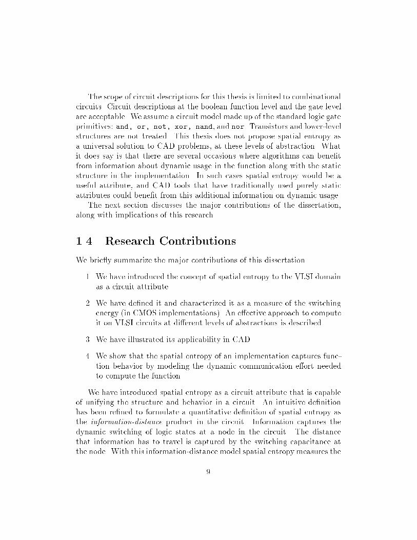
The scope of circuit descriptions for this thesis is limited to combinationalcircuits� Circuit descriptions at the boolean function level and the gate levelare acceptable� We assume a circuit model made up of the standard logic gateprimitives� and� or� not� xor� nand and nor� Transistors and lowerlevelstructures are not treated� This thesis does not propose spatial entropy asa universal solution to CAD problems at these levels of abstraction� Whatit does say is that there are several occasions where algorithms can bene�tfrom information about dynamic usage in the function along with the staticstructure in the implementation� In such cases spatial entropy would be auseful attribute and CAD tools that have traditionally used purely staticattributes could bene�t from this additional information on dynamic usage�The next section discusses the major contributions of the dissertation
along with implications of this research�
��� Research Contributions
We brie�y summarize the major contributions of this dissertation�
�� We have introduced the concept of spatial entropy to the VLSI domainas a circuit attribute�
�� We have de�ned it and characterized it as a measure of the switchingenergy �in CMOS implementations�� An e�ective approach to computeit on VLSI circuits at di�erent levels of abstractions is described�
�� We have illustrated its applicability in CAD�
�� We show that the spatial entropy of an implementation captures function behavior by modeling the dynamic communication e�ort neededto compute the function�
We have introduced spatial entropy as a circuit attribute that is capableof unifying the structure and behavior in a circuit� An intuitive de�nitionhas been re�ned to formulate a quantitative de�nition of spatial entropy asthe information�distance product in the circuit� Information captures thedynamic switching of logic states at a node in the circuit� The distancethat information has to travel is captured by the switching capacitance atthe node� With this informationdistance model spatial entropy measures the
�
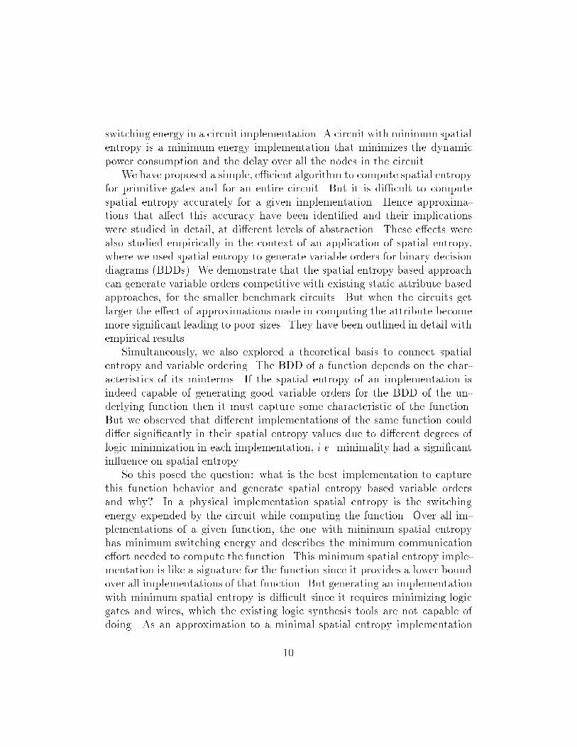
switching energy in a circuit implementation� A circuit with minimumspatialentropy is a minimum energy implementation that minimizes the dynamicpower consumption and the delay over all the nodes in the circuit�We have proposed a simple e�cient algorithm to compute spatial entropy
for primitive gates and for an entire circuit� But it is di�cult to computespatial entropy accurately for a given implementation� Hence approximations that a�ect this accuracy have been identi�ed and their implicationswere studied in detail at di�erent levels of abstraction� These e�ects werealso studied empirically in the context of an application of spatial entropywhere we used spatial entropy to generate variable orders for binary decisiondiagrams �BDDs�� We demonstrate that the spatial entropy based approachcan generate variable orders competitive with existing static attribute basedapproaches for the smaller benchmark circuits� But when the circuits getlarger the e�ect of approximations made in computing the attribute becomemore signi�cant leading to poor sizes� They have been outlined in detail withempirical results�Simultaneously we also explored a theoretical basis to connect spatial
entropy and variable ordering� The BDD of a function depends on the characteristics of its minterms� If the spatial entropy of an implementation isindeed capable of generating good variable orders for the BDD of the underlying function then it must capture some characteristic of the function�But we observed that di�erent implementations of the same function coulddi�er signi�cantly in their spatial entropy values due to di�erent degrees oflogic minimization in each implementation i�e� minimality had a signi�cantin�uence on spatial entropy�So this posed the question� what is the best implementation to capture
this function behavior and generate spatial entropy based variable ordersand why� In a physical implementation spatial entropy is the switchingenergy expended by the circuit while computing the function� Over all implementations of a given function the one with minimum spatial entropyhas minimum switching energy and describes the minimum communicatione�ort needed to compute the function� This minimum spatial entropy implementation is like a signature for the function since it provides a lower boundover all implementations of that function� But generating an implementationwith minimum spatial entropy is di�cult since it requires minimizing logicgates and wires which the existing logic synthesis tools are not capable ofdoing� As an approximation to a minimal spatial entropy implementation
��

we use a minimal gate count implementation� In order to study how spatialentropy on a minimal gate count implementation captures function behaviorwe started by de�ning minimality and spatial entropy computation in cubespace� This work also led to the second application of spatial entropy its useas a gatecount complexity measure for boolean functions�We �rst proposed an entropy based de�nition of the gatecount complex
ity of boolean functions called information content� Since the complexity of afunction is a measure that provides a lower bound on some physical attributeover all implementations of that function this captures a fundamental characteristic of function behavior� We also show that the information contentwhich is de�ned over a minimal Karnaugh decomposition of the functioncaptures minimality of twolevel function representations� This is becausethe minimal Karnaugh decomposition is equivalent to a minimized primeand irredundant twolevel representation of the function� Minimality formultilevel function representations was then de�ned using a notation calleddecision tree to relate a function to its implementation� An implementationis constructed bottom up from a decision tree and a minimal implementation corresponds to a minimal decision tree� Spatial entropy in cube spacewas then de�ned as the incremental contribution to the information contentover all nodes in an implementation derived from the decision tree� This definition of spatial entropy captures the communication between the mintermsin the implementation�We then empirically veri�ed that spatial entropy of a minimal implemen
tation does track function behavior in the form of the information contentof the function� While it is computationally intractable to compute the cubespace de�nition of spatial entropy we showed that the gatelevel spatial entropy computation procedure can be used as an approximation to it� Weshowed statistically that there is a strong correlation between the spatialentropy of a minimized implementation �as computed by the gatelevel procedure� and the information content of the function� Our de�nition of cubespace spatial entropy and information content was only de�ned for singleoutput completely speci�ed functions� So we handled multioutput functionsin our experiments by treating each of them as individual singleoutput functions�The information content of the function is de�ned over a minimal Kar
naugh decomposition and is thus an indicator of minimality in twolevelfunctions� We showed that the information content also estimates the gate
��

count complexity of a multilevel implementation of the function in terms ofthe logic gates required to implement it� An empirical correlation betweenthe information content and the gate count �in a multilevel implementation�is shown for several single output functions�The high degree of correlation between spatial entropy and information
content shows us that spatial entropy can be used to measure the gate countof a multilevel implementation of the function� We also found a strong correlation between spatial entropy and gate count for our experimental dataset� There is an explanation for this� Given that we limit our scope toonly combinational circuits the switching energy in these circuits is a function of the switching of states at the nodes and the delays at the nodes� Inmost combinational circuits this switching energy is equivalent to the circuitarea since almost the entire circuit is switching as the circuit computes dynamically� since spatial entropy measures switching energy we �nd the highcorrelation between spatial entropy and circuit area� This correlation wouldprobably be absent in sequential circuits where the switching energy is not adirect function of circuit area or in other combinational circuits where onlya fraction of the area is switched�Spatial entropy is a unique attribute since it is capable of capturing the
structure in an implementation and the behavior of the function being implemented� One can use the structural aspect of spatial entropy to discriminatebetween two implementations of the same function where an implementationwith lesser spatial entropy has lesser switching energy� Since a minimum spatial entropy implementation acts as a signature of the underlying functionone can compute this for two di�erent functions and compare the minimumswitching energies of these two functions� The fact that spatial entropy canmeasure information content a characteristic of the function that is invariant over di�erent implementations further lends credence to our hypothesisthat spatial entropy if computed accurately can generate good variable orders for BDDs on even the larger circuits� This is because BDDs too are acharacteristic of the function de�nitions and not of its implementations�
��� Dissertation Outline
In the next chapter we describe work that is related to our research� Thisis discussed along three directions� We �rst describe traditional static and
��

dynamic attributes in CAD and highlight the circuit properties that theycapture� Then we discuss approaches that estimate complexity in terms ofinformation �ow or wiring area when data has to be communicated betweenvarious places in a circuit� Finally we discuss entropy based attributes inCAD�In Chapter � we introduce the spatial entropy concept to the circuit
domain� It is �rst de�ned intuitively and then quantitatively as a dynamiccircuit attribute that measures the switching energy in a circuit� We showthat spatial entropy can be computed using existing circuit attributes andwe propose an algorithm to compute spatial entropy for primitive gates andfor an entire circuit� In the remainder of this chapter we characterize theattribute thoroughly explain why it is di�cult to compute it accurately andoutline the approximations that a�ect its accuracy�The subsequent chapters illustrate applications of spatial entropy� In
Chapter � we begin by introducing the variable ordering problem for binary decision diagrams �BDDs�� After a short survey of related research wedescribe our approach of using spatial entropy vectors to generate variableorders� The rest of the chapter describes our experiment to study spatial entropy based variable ordering empirically� The objectives are twofold� Firstwe study the e�ectiveness of spatial entropy in generating variable ordersand compare it with several existing approaches� Then we study the e�ectof the various factors and approximations and how they a�ect the accuracyof spatial entropy�Chapter � draws on the conclusions in Chapter �� It explains minimality
and spatial entropy in cube space� It also illustrates empirically how spatialentropy can measure the areacomplexity in boolean functions in terms ofthe multilevel gate implementations of these functions�Finally we summarize conclusions and future directions in Chapter ��
��

Chapter �
Related Work
The spatial entropy attribute has three characteristics its ability to unifystatic circuit structure and dynamic usage its ability to capture functioncomplexity and its information theoretic basis� We discuss related work inthis chapter by developing it along these three directions�First we brie�y describe traditional attributes that capture either static
structure or dynamic usage and discuss how they have been used to solveCAD problems� Our purpose here is to illustrate circuit properties that arecaptured by these attributes in order to contrast them later to the propertiescaptured by the spatial entropy attribute� In the second part of this chapterwe discuss approaches that estimate the complexity involved when data hasto communicate from various points in the circuit� The objective here isto illustrate how these approaches have been used to derive indicators suchas information �ow wiring area etc� to estimate this complexity� This willhelp us contrast them with the use of spatial entropy to capture wiring complexity and boolean function complexity which we discuss in later chapters�Finally we describe other entropy based attributes that rely on an information theoretic de�nition �like spatial entropy� and outline their applicationto problems in CAD�
��� Static and Dynamic Attributes
We begin by brie�y contrasting static and dynamic circuit attributes� Staticattributes are computed by examining the circuit structure or topology� In

contrast dynamic attributes are computed by exercising a circuit representation such that the circuit computes over a distribution of input values�While static attributes capture circuit connectivity or structure dynamicattributes capture usage of various parts of the circuit over a distributionof input data values� Static attributes can be usually computed quickly�dynamic attributes on the other hand can be expensive to compute� Wenow consider a subset of CAD problems and describe in turn the role staticand dynamic attributes play in solving them� We also highlight the circuitproperties captured by these attributes�Static attributes are typically used when information about the circuit
connectivity or structure is essential to solving the problem� Consider theproblem of timing analysis� The objective here is to identify the critical�or longest sensitizable� path in the circuit to estimate the worstcase delay�Since the actual delay along a path in the circuit depends on the propagationdelay and the number of gates in the path classical static timing analysis�Ous��� uses attributes like static gate depth and fanout along with propagation delay to arrive at an estimate of the worstcase delay� But this is notalways a true estimate� This is because some paths in the circuit are generated with subpaths that require input combinations that can never occur�These logically incompatible paths are called false paths and accumulatinggate delays along such paths would be erroneous� On the other hand anexact estimate of the critical path delay in the circuit would require simulating the circuit over all possible inputs to examine the e�ects of all inputcombinations� Since this is expensive the static attributes are used to obtain a quick approximation of the actual delay in terms of gate connectivityand gate depth� A lot of the work in timing analysis now concentrates oneliminating false paths �BI�� MK�� DYG�� BMCM�� PCD����Logic minimization and logic synthesis is another area of CAD where
solutions are guided by static circuit structure information� One of the objectives here is to map a twolevel boolean function representation into a setof gates �from some library� that occupies minimumarea �BHMSV�� BM��BRSVW�� LKB�� LBK���� Ideally one would like to achieve this objectiveof minimum area with respect to not just the gates in the circuit but also thewiring between them �Sau���� But since the notion of wires is absent at thelogic level of abstraction the objective is restricted to minimum gate area�The static circuit attribute of literal count becomes an approximation to thegate area� Hence algorithms in logic minimization and logic synthesis use
��
minimum literal count as the area criterion� Literal count is not only usedas a measure of performance of the algorithm but it is also used to guidethe algorithm during the minimization process� It assists in searching andselecting candidate factors for substitution while decomposing and factoringthe boolean function�Finally let us look at static attributes at the physical layout level� CAD
tools in the area of placement and routing are faced with the goal of placingcircuit components on a �dimensional plane and connecting nets betweenthem such that area and delay of the resulting circuit layout is minimized�LP���� Again static structure and connectivity information play an important role here� They are captured by attributes like wire length componentdimensions userde�ned or prerouted obstructions etc�� These yield minimization criteria such as minimum total net length minimum circuit areaminimum number of vias routeability for all nets prior routing of selected�power and ground� nets etc�� The algorithms are guided towards desiredsolutions by a suitably weighted version of these criteria�Dynamic attributes are typically used when circuit behavior over all pos
sible inputs needs to be captured to solve a problem� Simulation is one suchinstance� Regardless of the kind of simulation �function gate switch circuitfault� it is complete only when the circuit behavior for all possible inputs isstudied� In such a case the input vectors that represent various input combinations are dynamic attributes that capture circuit usage as they propagatethrough the various nodes�Testability analysis �BPH�� SDB�� JA�� LBdGG��� which is some
times viewed as an alternative to fault simulation is another problem thatrelies on a dynamic attribute� The objective here is to project the cost oftesting by predicting the number of random test patterns needed to achievehigh fault coverage� High fault coverage is usually de�ned by predicting alarge percentage ��� � �� � of faults in the circuit with a high probability����� � ������ To solve this problem the probability of detecting a fault isexpressed as a function of two probability based attributes� observability andcontrollability� Controllability is computed by assigning signal probabilitiesat the inputs to the circuit and propagating them forward through all thenodes in the circuit� Observability is computed similarly except that it iscomputed backwards from the output� These probability based attributesare dynamic because they capture circuit usage over di�erent input combinations� In this particular instance they are being used to detect a given
��

list of stuckat faults �at nodes in the circuit� by looking at the value ofthe node over all possible input combinations� We now look at research incommunication complexity�
��� Communication Complexity Prediction
With VLSI design being performed in submicron technology with smallerfeature sizes there is a realization that the areatime and power performanceof a circuit will be dominated less by the logic or the gates in the circuitand more by the wires and the communication between the logic� This hasresulted in e�orts to estimate communication complexity by the wiring areaor information �ow in a circuit�In ���� Thompson introduced a model �Tho��� for computing lower
bounds on the complexity of VLSI implementations of functions� The complexity of the computation was measured in terms of bounds �AT � A�T ��on chip area and computation time� The model highlighted the di�culty ofcommunicating information across the surface of a chip� Given any partitionof the input set into two equal halves on two disjoint regions of the chip theseareatime bounds de�ned lower bounds on the communication complexity ofthe function�The notion of communication complexity across a partition was intro
duced by Yao to provide lower bounds on the worst case information complexity of many functions �Yao���� Yao!s model assumed a particular partitioningof the input set into two equal halves �as against the VLSI complexity modelthat assumes any partition�� This captured a local information �ow acrossthe partition� The communication complexity was de�ned as the number ofbits of information that needed to cross the partition to correctly computethe function� These bits of information were computed by a twoway protocol that dictated how the bits would be exchanged by the two input halves�The maximum number of bits exchanged over all input values for computingthe function f was de�ned as the communication complexity c�p� for a givenprotocol p� The worstcase complexity was then de�ned as the minimumtwo�way communication complexity over all protocols for that partition�More recently Hwang Owens and Irwin �HOI�� HOI��� have used com
munication complexity for multilevel logic synthesis� They have also provided ways to compute the communication complexity whose bounds were
��

estimated in �Yao���� In their approach the �decomposition and factoring�operations in multilevel logic minimization are performed by partitioningthe boolean function f into three functions ft� fl� fr such that
f�X� � ft�fl�Xl�� fr�Xr��
whereXl and Xr denote a disjoint partition of the input setX �Xl�Xr � X��The partition is generated using heuristic partitioning techniques that try tominimize the communication complexity or the number of interconnectionsbetween the functions �ft� fl� and �ft� fr�� The communication complexityfor a given partition which acts as a cost function for their partitioning algorithm is computed by computing the number of compatible classes �Ris���of a given function� Two approaches were illustrated� The �rst approach usesa communication matrix while the second approach which is more e�cientuses cubes and cube overlaps �BHMSV����Another partially related approach is discussed in �ASSP���� Here wiring
complexity in a synthesized circuit is minimized by controlling input dependency with lexicographic expressions of a boolean function� A lexicographicexpression of a boolean function is a sum of product terms in which the inputliterals �that every product term depends upon� conform to an ordering calledthe reference order� This ordering is used to extract a set of lexicographicallycompatible kernels �BM���� Kernel �ltering computes the intersection of theextracted kernels to �nd shared parts amongst the functions� By tightlycontrolling this �ltering process the logic cones can be prevented from intersecting with each other� The objective is to reduce the wiring between logiccones that manifests itself as wires in the layout�We now discuss the application of entropy based attributes in CAD�
��� Entropy Based Attributes
����� Background
We begin with some background on the concept of entropy� There are twopopular de�nitions of entropy� Information theory �SW��� de�nes it as themeasure of information content in a system� Thermodynamic �Sea��� de�nesit as the thermodynamic probability of the internal particles of a systemwhile holding the external properties constant� We consider each de�nition
��

in turn and show how they both view entropy as � the measure of disorderin a system��Consider a system with N possible output events� In information theory
this is usually a communication system where the N events are messages tobe communicated to a receiver� Suppose each event i has a certain probabilityof occurrence pi with respect to its inputs� Then the informationtheoreticde�nition of entropy is the measure of information produced when one eventis chosen from this set N �SW���� It is de�ned as
Xi�N
pi log�
pi
When all the events are equally likely i�e� pi ��N the expression reduces to
logN �As an example consider a system where the messages are represented
by a bit string of length n� The set of output events N is the set of allpossible messages that can be represented by the nbit string� If all bitcombinations are assumed likely then the nbit string can represent at mostN � �n di�erent messages� On the other hand suppose we insisted that onlya single bit combination that of all �s in the string is possible� Then onlyone message �N � �� will be possible� In the former case the informationcontent �entropy� of the bitstring is log��n� � n while in the latter caseit is log��� � �� Thus if greater number of bit combinations �or messages�are possible this implies greater disorder in the system� This in turn impliesgreater entropy or information content�In the same vein a bitstring that is twice as long � of length �n� will
have an information content �or entropy� equal to �n� This conforms to ourintuitive notion that a message that is twice as long should be able to containtwice as much information�In thermodynamics entropy is de�ned as being proportional to the log
arithm of the number of ways of arranging the particles in a system whilemaintaining external conditions constant� As an intuitive example �MC���consider a system with two containers holding a total of �� red and �� bluemolecules� If we do not distinguish between containers there is only one wayin which the molecules can be arranged so that all the �� blue ones are in onecontainer and all the �� red ones in the other� On the other hand there area large number of ways of arranging � of each color in each container� The
��

second arrangement of molecules has much more disorder than the �rst andtherefore has much more entropy than the �rst� The actual de�nition �Sea���of this entropy S is in terms of the thermodynamic probability of the internalparticles in the system� It is de�ned as S � k logW where k is Boltzman!sconstant and W is the thermodynamic probability�Thus in both information theory and thermodynamics entropy captures
the measure of disorder in a system� The informationtheoretic de�nition ofentropy has found applications in a few areas of CAD� We begin by reviewingwork in these areas�
����� The Entropy function in CAD
One of the �rst applications of information theory was to use the informationtheoretic de�nition of entropy to predict boolean function complexity� Therelationship between function complexity and entropy was �rst conjecturedby Cook and Flynn �CF���� The complexity of a boolean function is expressedby the cost of implementing the function as a combinational network� Cookand Flynn demonstrated empirically that the average cost behavior of a singleoutput combinational network could be modeled by a formula that capturedthe entropy of the boolean function implemented by the network� It wasde�ned as
H�f� �u
�nlog�
�n
u��n � u
�nlog�
�n
�n � u
where n is the number of input variables and u is the number of ONtermsin the cube space� Subsequently Hellerman �Hel��� proposed a de�nitionof computational work based on the entropy function� Suppose a functionf � X � Y performed some computation over a domain of inputs X and arange of outputs Y � fy�� � � � � yng� Then for Xi � X and Xi � f���yi� the
work done by the function was expressed asPn
i��j Xi j log jXj
jXijwhere j X j
denotes the number of elements in the set�The relationship between the works of Hellerman and Cook � Flynn
was later observed by Mase�Mas���� He showed that the complexity of aboolean function can be expressed in terms of an entropybased de�nition of�computational� work performed by the combinational network�In ���� Pippenger further re�ned this entropy de�nition to handle don!t
cares in the function �Pip���� More recently in �CA��� the entropy formulation was generalized to multioutput functions both completely speci�ed
��

functions and partially speci�ed ones� They also showed statistically thatusing the literal count as a measure of circuit area a linear relationship canbe observed between entropy and average number of literals in a multilevelimplementation�Information theory has also found application as a testability measure�
This was �rst proposed by Dussault �Dus���� He presented observability andcontrollability measures based on information theory for gate level circuits�In �TA��� Thearling and Abraham extended this idea to estimate testabilityat the function level� They use a measure called the information transfer coe�cient �ITC� �Koo��� to enable relative testability measures to be computedas against the absolute measures computed by Dussault �Dus���� Agrawal�Agr��� has also applied information theory to test pattern generation� Heshows that by choosing test patterns that maximize the information at theoutput the probability of fault detection can be maximized�
����� Entropy as a basis for Computation
In �MC��� Carver Mead proposed the idea of computation based on entropy�This has formed the basis for our de�nition of spatial entropy in the circuitdomain that we discuss in Chapter ��He begins by suggesting that computation can be viewed as a process
that reduces the disorder �or entropy� in the solution space while arrivingat a result� Every computation �nds an answer by making decisions on asolution space� With each decision the usually huge initial solution spaceis cut down to some fraction of its former size� The number of decisionsrequired to specify one correct answer in the solution space is the entropyof the computation de�ned as log jTotal Solnsj
jAnswerj � This de�nition is analogous
to the informationtheoretic de�nition of entropy where the solution space isall possible messages with a given length and bitstring format� The correctanswer is one such message and the entropy is the number of bits requiredto specify this correct answer�The description of entropy outlined above captures algorithmic compu
tation and Mead terms this as logical entropy� This is because it depends onthe logical operations required to perform the computation� The objective ofa computation is to reduce the logical entropy of the data to zero� The studyof algorithm complexity analysis is the study of these logical operations modeled by logical entropy� Mead also proposes another form of entropy called
��

spatial entropy that is usually seen in situations when the computation hasto be mapped onto a domain where data travels over a physical distance� Thecontrast between the two forms of entropy is best captured by the followingquote from �MC��� �
� In any physical system� the logical entropy treated by classicalcomplexity theory is only part of the story� There is also a spatialentropy associated with a computation� Spatial entropy may bethought of as a measure of data being in the wrong place� justas logical entropy is a measure of data being in the wrong form�Data communications are used to remove spatial entropy� just aslogical operations are used to remove logical entropy��
Entropy is the measure of disorder in a system� So spatial entropy isthe measure of spatial disorder in a system� This spatial disorder �or spatialentropy� in a system captures a form of spatial distance between the inputsand the outputs in a system� The spatial entropy S of a system quanti�esthe spatial e�ort needed to bring the data at the input location to the outputlocation� When a system computes the data communications in the systemare carrying data from the input to the output� This reduces the spatialdistance between them or removes spatial entropy in the system�One scenario that illustrates spatial entropy is a communication network�
Here messages or communication events are transmitted over communication pathways that remove spatial entropy by routing data between variousspatially distributed source and destination sites� Another example is circuitcomputation� Here the input data travels through the wires in the circuit�These wires remove spatial entropy in the circuit by carrying the input datato the outputs� It is this latter model that is of interest to us� In the nextchapter we characterize the spatial entropy concept in the circuit domain andde�ne a quantitative measure that relates it to the switching energy in thecircuit� We describe an algorithm that computes spatial entropy for a gatelevel circuit implementation and study the factors a�ecting the accuracy ofthis computation�
��
Chapter �
Spatial Entropy � A Circuit
Attribute
In the previous chapter we introduced the concept of spatial entropy�In this chapter we illustrate how spatial entropy can be characterized as adynamic attribute in the circuit domain� We de�ne spatial entropy quantitatively and show how it can be computed on primitive gates and overan entire circuit� We also explain how it measures the switching energy ina physical implementation� Computing the attribute accurately is unfortunately a di�cult task and there are di�erent factors that a�ect its accuracy�In the latter part of this chapter we discuss these factors in detail and explainhow they result in various approximations while computing the attribute�We begin with an intuitive notion of circuit spatial entropy followed by
a quantitative de�nition� In Section ��� the technique to compute spatialentropy for gate level primitives is described� This becomes the basis for analgorithm to compute circuit spatial entropy which we outline in Section ����Section ��� further characterizes the attribute by introducing spatial entropyvectors� In Section ��� we talk about the di�culties in computing this attribute accurately and how these factors force approximations to be madeduring spatial entropy computation�

��� Introduction and De�nitions
Spatial entropy can be intuitively de�ned as the communication e�ort required to compute the circuit function� In a circuit both the logic gatesand the wires contribute e�ort towards computing the circuit function� Thegates compute boolean values or bits and the wires transmit these bits� Spatial entropy models the dynamic communication taking place in the circuitversus the static communication modeled by the wires� Over all the inputcombinations it tries to capture the distribution of bits at the gate outputsand the communication of these bits from one gate output to another� Whilethe wires determine how far the bits have to travel the gate types determinethe distribution of boolean values that these bits take at the various nodesin the circuit� Together they determine the dynamic communication e�ort inthe circuit� We use an informationtheoretic de�nition to capture this e�ortthrough the circuit�We start with a description of our circuit model� A circuit is represented
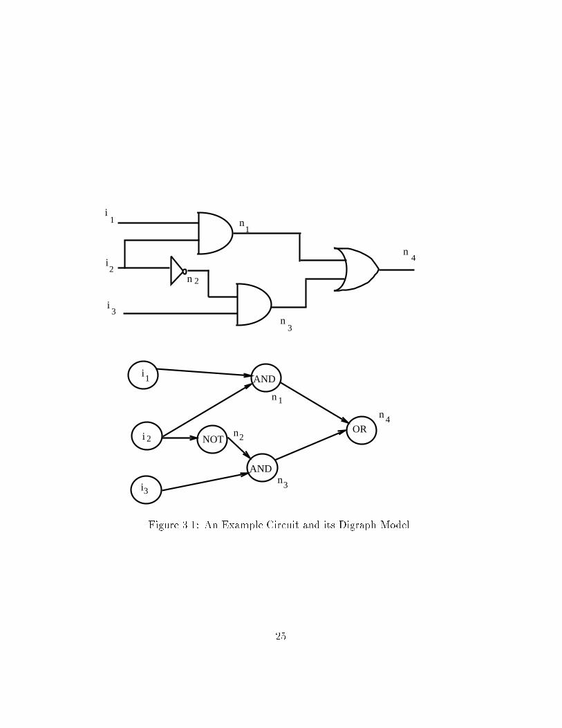
as a directed weighted graph G � hV�E�Li� Each primary input primaryoutput and logic gate in the circuit is represented by a node v � V in thegraph� An edge �v�w� � E represents a wire in the circuit� Each such edgehas a length attribute l�v�w� � L that is the length of the wire� L � E � Rwhere R is the set of real numbers� The direction of the edge from v to wrepresents the direction in which the bits travel in the wire� v is the sourcenode and w is the destination node for the edge� The directed edges from vto other nodes are called fanout edges� v is the source node of these edgesand the bits leave from v along these edges to go to destination fanout nodes�The directed edges that come into node v are called fanin edges� v is thedestination node of these edges and the bits enter v along these edges fromsource fanin nodes� The primary input nodes have no fanin edges and theprimary output nodes have no fanout edges� The number of fanin edges of agate node is equal to the number of inputs to the gate� A path in the graph isa sequence of vertices from a source node to a destination node� The supportset of a node v is the set of all primary inputs from which there is a path tonode v� Figure ��� illustrates a simple circuit and its corresponding directedgraph model� �The edge lengths are not shown��We now re�ne the idea of dynamic communication e�ort by quantifying it
with circuit attributes� To capture the distribution of boolean values at thenode we use the classical entropy function H�fpig� from information theory
��
i
i
i
1 n
n
n3
2
1
4n
2
3
AND
AND
ORNOT
i
i
i
n
n
n
n
1
2
3
2
1
3
4
Figure ���� An Example Circuit and its Digraph Model
��
�SW���H�fpig� �PN
i��pi log�
�pi�� N represents the number of possible values
�or events� in a given system� Since there are only two values possible in adigital circuit we can model the distribution of boolean values computed ata node w by the binary entropy function H�fp�
w� p�
wg� at the node
H�fp�w� p�
wg� � p�
wlog�
�
p�w
� � p�wlog�
�
p�w
�
where p�wis the �probability of a node w and p�
w� �� � p�
w� is the �
probability of the node� The probability of a node gives the distributionof � and � values computed by the node� This binary entropy functionH�fp�
w� p�
wg� denotes the information computed at the node over this proba
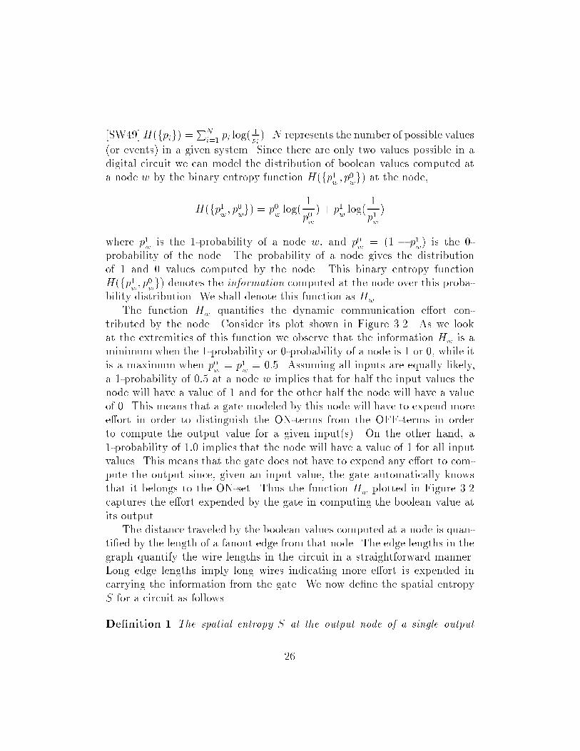
bility distribution� We shall denote this function as Hw�The function Hw quanti�es the dynamic communication e�ort con
tributed by the node� Consider its plot shown in Figure ���� As we lookat the extremities of this function we observe that the information Hw is aminimumwhen the �probability or �probability of a node is � or � while itis a maximum when p�
w� p�
w� ���� Assuming all inputs are equally likely
a �probability of ��� at a node w implies that for half the input values thenode will have a value of � and for the other half the node will have a valueof �� This means that a gate modeled by this node will have to expend moree�ort in order to distinguish the ONterms from the OFFterms in orderto compute the output value for a given input�s�� On the other hand a�probability of ��� implies that the node will have a value of � for all inputvalues� This means that the gate does not have to expend any e�ort to compute the output since given an input value the gate automatically knowsthat it belongs to the ONset� Thus the function Hw plotted in Figure ���captures the e�ort expended by the gate in computing the boolean value atits output�The distance traveled by the boolean values computed at a node is quan
ti�ed by the length of a fanout edge from that node� The edge lengths in thegraph quantify the wire lengths in the circuit in a straightforward manner�Long edge lengths imply long wires indicating more e�ort is expended incarrying the information from the gate� We now de�ne the spatial entropyS for a circuit as follows�
De�nition � The spatial entropy S at the output node of a single output
��

H
1.0
0.0p=0.0 p=1.0
p=0.5w
Figure ���� The Entropy Function Hw
circuit is the information�distance product over all the nodes in the circuit�
S �Xv�V
Xw�V
Hv � l�v�w�
Hv is the information computed at the node v over its input probability dis�tribution� and l�v�w� is the length of the fanout edge �v�w� � E� from node vto node w�
The spatial entropy S of a multioutput circuit is expressed as S �Pmi��
Soi where m is the number of outputs and Soi is the spatial entropy atoutput oi�At each node v the spatial entropy is computed by multiplying the in
formation computed at v by the distance it has to travel along all the fanoutedges from v� With this de�nition the intuitive notion of communicatione�ort is captured by the total information �ow in the circuit� The nodescompute the information while the edges communicate this information�How does spatial entropy capture dynamic circuit usage� Spatial entropy
is a dynamic circuit attribute in the sense that its value computed fromthe entropy function H is a function of the probability distribution at theprimary inputs of the circuit� Thus H captures circuit usage de�ned by thisprobability distribution� Since it is symmetric it gives an accurate modelof circuit usage capturing the propagation of both � and � probabilities� Acircuit that propagates mostly �s in its internal nodes could still be performing useful computation� but this would not be captured well with only�probabilities�
��

This de�nition of spatial entropy as the informationdistance product isa good model to measure the switching energy in a physical circuit implementation� The switching energy of a device is de�ned as the dynamic powerconsumed by the device multiplied by the delay associated with the device�It gives a measure of the dynamic work performed by the device� In CMOSimplementations the switching power Psw depends on the frequency at whichthe circuit runs and the number of times the switching capacitance Csw getscharged and discharged while the nodes switch logic states �� � �� � ���The delay is the time taken to charge or discharge the capacitance associated with a node and it is a function of the resistance and capacitance ofthe device and the wiring associated with it�In a physical implementation the information at a node �computed by
the entropy function Hw� captures the dynamic switching of logic states atthe node� A node with high information has equal likelihood of acquiringa value of � or � �p � ����� This also implies that such a node is likely toundergo more switching of states ��� ��� �� during dynamic computationand thus expend more switching energy� The distance information has totravel is a measure of the switching capacitance that needs to be chargedand discharged since this determines the delay incurred before the nodechanges state� Long edge lengths imply high switching capacitances causinglonger delays for a node to change state and longer delays for informationto travel to the next node� This de�nition of spatial entropy thus provides aquantitative measure for the switching energy in a physical implementation�In the next section we describe a way to estimate spatial entropy in a
circuit� It is di�cult to compute spatial entropy accurately and we onlyillustrate how to compute approximations to the spatial entropy de�nitionin De�nition �� We begin by describing this process for individual primitivegates that then evolves into a procedure to compute spatial entropy for anentire circuit�
��� Spatial Entropy Computation
We restrict our treatment of spatial entropy computation to the domain ofcombinational circuits at the gate level� Spatial entropy of sequential circuitscan be computed by expressing their next state and output functions asblocks of combinational logic� In this case the spatial entropy computation
��

will capture the information �ow through the circuit for only a single clockcycle� This would have to be repeated over successive clock cycles with newprobability values to capture the entire computation of the sequential circuit�The circuits are multilevel implementations and technology mapping mayor may not have taken place�We begin by describing spatial entropy computation for implementations
of single output boolean functions� Subsequently we extend our procedureto compute the spatial entropy of multioutput implementations� In order tocompute spatial entropy for circuits at the gate level the spatial entropy forprimitive logic gates needs to be de�ned� Spatial entropy is a function of theinformation Hw at a node and the fanout edge length at the node� But edgelengths are absent at the gate level� We currently assume unit edge length inour graph i�e� unit wire length in our circuit and compute an approximationto the spatial entropy of the circuit� Later in this chapter we describe waysto re�ne this approximation by obtaining estimates of the edge length�The local spatial entropy at a gate node g � V is de�ned as�
�Sg �Xg��V
Hg � l�g�g��
where Hg is the information computed at the gate node g and l�g�g�� is thelength of the fanout edge from node g to node g�� Since we have assumedl�g�g�� � � we can only compute an approximation �Sg � Hg� We illustratethis for some simple �input gates�Consider a �input AND gate with �probabilities of p�
xp�yat its inputs
x� y� The �probability at the output of the AND gate is p�and
� p�x� p�
y
since the only event yielding a � at the output is p�x� p�
y� The local spatial
entropy at the AND gates �Sand is equal to the information at the gateHand � p�
andlog �
p�and
� p�andlog �
p�and
�
For a �input XOR gate the �probability p�xor� p�
y��� p�
x� � p�
x��� p�
y�
since there can be a � at the output only if x � � and y � � or y � � andx � �� The local spatial entropy �Sxor � Hxor where Hxor � p�
xorlog �
p�xor�
p�xorlog �
p�xor�
For a �input OR gate the �probability p�or� � � �� � p�
x���� p�
y�� This
is obtained by subtracting from � the probability of the event that wouldyield a � at the output� Similarly the local spatial entropy �Sor � Hor whereHor � p�
orlog �
p�or� p�
orlog �
p�or�
��

For a NOT gate the �probability p�notis equal to � � px and the �
probability p�notis equal to px� The local spatial entropy �Snot � Hnot is
p�notlog �
p�not�p�
notlog �
p�not� The local spatial entropy values for �input NAND
NOR and other ����multiinput �ANDOREXOR� gates can be computedsimilarly�To see what these de�nitions mean let us assume for the moment that
the �probabilities at the inputs of all the above gates are ��� that is � and� are equally likely at the inputs� Then the �probabilities ��probabilities�at the outputs of the above gates are AND���������� OR���������� XOR�������� and NOT��������� Computing the information content H of theseprobability distributions we discover that the AND and OR gates will havethe same amount of information� This is because both have the same distribution of � � events at the output� In the AND three input events yieldsa � and one input event yields a � at the output� It is exactly the reversein the OR gate� In the case of NOT and XOR gates assuming an inputprobability of ��� both gates have the same amount of information H � ��This implies maximum information� The reason for this is that both gateshave equal probabilities for output events of � and � and thus the outputhas as much chance of being a � as being a ��We now have rules to compute the spatial entropy for the primitive gates
in our circuit� What is now needed is a way of accumulating these spatial entropy values over the various nodes in the combinational circuit� This wouldgive us the spatial entropy at the output of the circuit� We illustrate thiswith a simple example �rst and then describe a simple algorithm for spatialentropy computation� As we indicated before this computes an approximation to the actual spatial entropy since we assume unit edge lengths� In aphysical implementation such an approximation to spatial entropy will yielda measure of the dynamic power consumed in a circuit� It captures the rateat which the switching capacitance at each node charges and discharges asthe logic states change at the nodes without capturing the delay associatedwith the node�Consider the example combinational circuit in Figure ���� The circuit has
� inputs and � output� We assume the input values are distributed such thateach input has equal probability of being a � or �� So the circuit is initializedby assigning all primary inputs with a probability of ���� This initializesthe spatial entropy of every primary input to ��� �p � ��� �� H � ��� ��
��
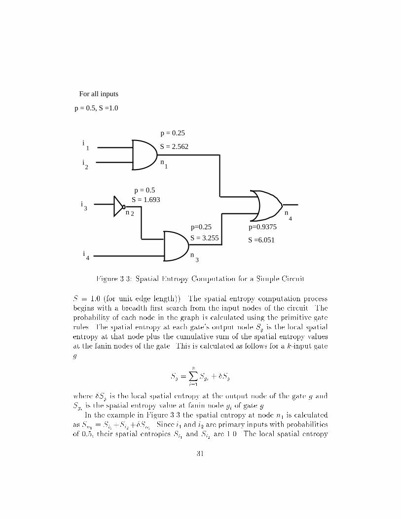
For all inputs
p = 0.5, S =1.0
S = 1.693
p=0.25 p=0.9375
S = 3.255 S =6.051
i
i
i
1
n
n
n3
2
1
4n
2
3
i4
p = 0.5
S = 2.562
p = 0.25
Figure ���� Spatial Entropy Computation for a Simple Circuit
S � ��� �for unit edge length��� The spatial entropy computation processbegins with a breadth �rst search from the input nodes of the circuit� Theprobability of each node in the graph is calculated using the primitive gaterules� The spatial entropy at each gate!s output node Sg is the local spatialentropy at that node plus the cumulative sum of the spatial entropy valuesat the fanin nodes of the gate� This is calculated as follows for a kinput gateg�
Sg �kXi��
Sgi � �Sg
where �Sg is the local spatial entropy at the output node of the gate g andSgi is the spatial entropy value at fanin node gi of gate g�In the example in Figure ��� the spatial entropy at node n� is calculated
as Sn� � Si��Si���Sn� � Since i� and i� are primary inputs with probabilitiesof ��� their spatial entropies Si� and Si� are ���� The local spatial entropy
��

at n� �Sn� is calculated using the formula for an AND gate to yield �Sn� �����log� �
���������log� �
��� � ������ Similarly Sn� � Si���Sn� � ������ The
spatial entropy at the internal node n� is calculated as Sn� � Sn��Si���Sn��In this case while Si� � ��� Sn� � ������ �Sn� is calculated as it is calculatedfor n�� Therefore Sn� � ��� � ����� � ����� � ������ Finally the spatialentropy at the output node n� is calculated to obtain a value for the totalspatial entropy of the circuit� Sn� � ����� � ����� � �Sn�� The local spatialentropy at n� is calculated as ������ � log� �
������ ����� � log� �
������ � ������
This gives Sn� � ������In the next section we describe an algorithm to compute spatial entropy
for a given combinational circuit�
��� Algorithm
The following algorithm computes the spatial entropy for a given combinational circuit� The computed spatial entropy is an approximation to thespatial entropy in De�nition � since we have assumed unit edge lengths in thecircuit� The same algorithm can also be used to compute spatial entropy ifthe actual edge lengths or edge length estimates are available� We illustratethis later when discussing di�erent estimates of the edge length�We �rst describe the procedure informally and then outline the algorithm�
The input is a logic gate level description of a combinational circuit modeledas a connected directed graph �V�E�� The algorithm itself can �t in theframework of any eventdriven system� It performs a breadth�rst traversalof the graph by visiting nodes in successive levels� At the outset the levelis � and the only nodes visited are the primary input nodes� These areinitialized with their probability and spatial entropy values� The procedurethen collects all nodes that are reachable from them� This makes up thenodes at the next level� A gate node is added to a level only if all its faninnodes have been visited� The spatial entropy and probability values for thesenodes �at the next level� are calculated and the nodes are merged with theexisting set of visited nodes� The search then proceeds to the next level tocollect the next set of gate output nodes� This continues till all the nodes inthe graph have been visited �or reached�� This indicates breadth�rstsearchis complete� At this point the spatial entropy and probability values of allthe nodes have also been calculated� Shown below are some de�nitions and
��
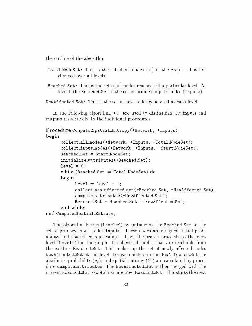
the outline of the algorithm�
Total NodeSet� This is the set of all nodes �V � in the graph� It is unchanged over all levels�
Reached Set� This is the set of all nodes reached till a particular level� Atlevel � the Reached Set is the set of primary inputs nodes �Inputs��
NewAffected Set� This is the set of new nodes generated at each level�
In the following algorithm ��� are used to distinguish the inputs andoutputs respectively to the individual procedures�
Procedure Compute Spatial Entropy��Network� �Inputs
begincollect all nodes��Network� �Inputs� �Total NodeSet�collect input nodes��Network� �Inputs� �Start NodeSet
Reached Set � Start NodeSet
initialize attributes��Reached Set
Level � �
while �Reached Set � Total NodeSet dobegin
Level � Level � �
collect new affected set��Reached Set� �NewAffected Set
compute attributes��NewAffected Set
Reached Set � Reached Set � NewAffected Set
end while�end Compute Spatial Entropy
The algorithm begins �Level��� by initializing the Reached Set to theset of primary input nodes Inputs� These nodes are assigned initial probability and spatial entropy values� Then the search proceeds to the nextlevel �Level��� in the graph� It collects all nodes that are reachable fromthe existing Reached Set� This makes up the set of newly a�ected nodesNewAffected Set at this level� For each node v in the NewAffected Set theattributes probability �pv� and spatial entropy �Sv� are calculated by procedure compute attributes� The NewAffected Set is then merged with thecurrent Reached Set to obtain an updated Reached Set� This starts the next
��

level of the breadth�rstsearch� This process repeats till the Reached Set
contains all the nodes in the graph �Total Node Set� indicating that breadth�rstsearch in the graph is complete�The run time of the algorithm depends on the number of nodes n in the
combinational circuit� Since the entire graph is connected in the worst casethe breadth �rst search will add at least one new node for each iteration ofthe while loop� Thus there will be at most n iterations of the loop�The frontier nodes Fl of the Reached Set at some level l consist of
all nodes that were added at level l � �� In order to generate theNewAffected Set at level l we examine the fanout nodes F �f� from eachfrontier node f � Fl� Only a subset of nodes F ��f� � F �f� are eligible toenter the NewAffected Set� Nodes whose fanins are not in the Reached Set
are discarded from F �f�� For a pair of frontier nodes f� g � Fl the eligiblefanout sets F ��f�� F ��g� are not necessarily disjoint� Two nodes can fanoutto the same node at the next level� Hence we need a union to compute theNewAffected Set� At level l NewAffected Set � �f�Fl
F ��f�� In the worstcase an F ��f� can be the entire set of nodes n� So the NewAffected Set iscollected as an ordered set �without duplicates� and the union operation �is implemented as an ordered set union whose total cost is the cost of sorting�to order the sets� followed by the cost of merging the two ordered sets�While the sorting requires O�n log n� time the merging can be done in timeproportional to the sum of the sizes of the two ordered sets �O�n��� Sincethe union is invoked for each level of the breadth �rst search the algorithmhas a worstcase run time complexity of O�n� log n��The above algorithm computes an approximation to the spatial entropy
of a combinational circuit� The same algorithm can be used to compute theactual spatial entropy as de�ned in De�nition � if edge length informationwere available� The only change would be to the compute attributes procedure that computes the local spatial entropy at each node in the circuit�In the next section we introduce spatial entropy vectors by extending the basic spatial entropy computation algorithm to further characterize the spatialentropy attribute�
��
��� Spatial Entropy Vectors
The spatial entropy of a circuit is a measure of the communication e�ortrequired to compute the circuit function� We obtained this amount by accumulating the spatial entropy at the internal nodes in the circuit� We can goone step further and characterize the spatial entropy of the circuit and thespatial entropy at the internal nodes of the circuit in terms of spatial entropycontributions of the primary inputs� This will give us the e�ort contributedby each primary input in computing the circuit function� In Chapter � weuse this idea to study the problem of variable orderings for binary decisiondiagrams �BDDs��We begin with an outline of the approach� The extension to the spatial
entropy computation procedure to capture spatial entropy contributions ofthe primary inputs is implemented by adding another attribute called thespatial entropy vector to each node in the network� The spatial entropy vectorat any node is an nelement vector containing the spatial entropy contributionof each of the n primary inputs to the spatial entropy at the node� The samealgorithm outlined in ��� is used to compute the spatial entropy vector at thecircuit outputs� The value of this vector at any internal node w is computedby adding the spatial entropy vectors at the node inputs to the local spatialentropy �Sw at the node� Since �Sw is a single value it is distributed amongstall the primary inputs in proportion to the spatial entropy contribution ofeach primary input at the fanins of node w� The spatial entropy contributionof each primary input at node w!s fanins can be computed from the spatialentropy vector at each of these fanins� We now express this idea formally�For a circuit with n primary inputs the spatial entropy at a node w Sw
and the spatial entropy vector at the node �Sw are related as follows
Sw �nX
j��
�Sw�xj�
The spatial entropy at the node is the cumulative sum of the spatial entropycontributions of each primary input at the node�
The spatial entropy vector at each primary input xj�Sxj consists of �s
at all input positions in the vector except for position j which contains a�� This indicates that the spatial entropy at this node is entirely contributedby the primary input xj�
��

.. . .
.
..
..
w..
Sw1
Swi
Swk
Sw
Figure ���� Spatial Entropy Vector Computation
How is the spatial entropy vector �S computed at a node w� The spatialentropy vectors at the k fanins of a node w �Figure ���� can be accumulated
by adding them together to obtain��
Sinw�Pk
i���Swi� This yields a single
accumulated vector consisting of the spatial entropy contributions of theprimary inputs to all the fanins of node w� Since the local spatial entropy atw �Sw is a single value it needs to be distributed as contributions over allthe primary inputs� This is accomplished by distributing �Sw amongst each
primary input in proportion to its value in the accumulated vector��Sinw� If
the total spatial entropy contribution of primary input xj over all the fanins
of node w is��Sinw �xj� and Sinw �
PNj��
��Sinw �xj� is the total spatial entropy
over all the fanins of node w then the local spatial entropy contribution ofprimary input xj is given by
�Sw ���
Sinw �xj�
Sinw
The intuitive justi�cation behind this step is as follows� The local spatialentropy at node w ��Sw� is a measure of the e�ort required to compute thevalue at w� We distribute this e�ort amongst the primary inputs using thereasoning that a primary input that has contributed more e�ort to the inputsof w will be rewarded by receiving a greater contribution of the local spatialentropy� This gives us the equation for computing the spatial entropy vector
��

at node w�
�Sw ���Sinw ��
�SwPNj��
��
Sinw�xj��� ��Sinw �����
If we now extend the algorithm so that it computes the spatial entropyvectors during the breadth �rst search we can obtain spatial entropy vectorsat the outputs that re�ect the spatial entropy contributions from the primary inputs� The following example will illustrate this extended algorithmon a simple gatelevel network� It must be mentioned again that since wehave assumed unit edge lengths only an approximation to the actual spatialentropy vectors is being computed in this example�Consider the combinational network shown in Figure ��� The circuit has
� inputs and � output� We assume that the input values are uniformlydistributed i�e� all inputs have �probability of � �� The spatial entropyvalues at all the input nodes Si�� Si�� Si�� Si� � ����The spatial entropy vector at each input is initialized to a vector that has
zeros at all positions and a ��� at that input position� �Si� � ����� ���� ���� �����Si� � ����� ���� ���� ����
�Si� � ����� ���� ���� �����Si� � ����� ���� ���� ����
The �rst level of the breadth�rstsearch yields nodes n and n in theNew Affected Set� So we compute the �probabilities and spatial entropyvalues at these nodes� n is the output of an OR node hence the �probabilityat n is � � �� � �"� ��� The �probability at n is � � since it is the outputof an inverter node� At n the spatial entropy value is calculated as follows
Sn� � Si� � Si� � �Sn�
The terms Si� and Si� provide the spatial entropy value from the inputsi� and i� which in this case is ���� �Sn� provides the local spatial entropycontribution at the OR node n� This works out to ������ Hence Sn� � ������Similarly Sn� � ������The spatial entropy vector at node n is
�Sn� ��Si� � �
�Sn�Si� � Si�
� � �Si� ��Si� � �
�Sn�Si� � Si�
� � �Si�
Here �Si� ��Si� are the initialized input vectors since i� and i� are inputs�
The other terms are calculated as follows� The term�Sn�
Si��Si�is the proportion
��

i
i
i
1
n
n
n
n
2
3
i4
5
S
8
9
n10
11
S = [1.281, 1.281, 0, 0 ]
S = 2.562
p = 0.75
p = 0.375
S = 4.224
S = [1.519, 1.519, 1.186, 0]
p = 0.5
S = 1.693
S = [0, 0, 1.693, 0]
p = 0.25
S= 3.256
S = [0, 0, 2.047, 1.209]
p = 0.5312
S = 8.17
= [1.66, 1.66, 3.53, 1.32]
Figure ���� Example Spatial Entropy Calculation ij j � �� �� pij � ���� Sij � ����
�Sij is a vector of
zeros� with a ��� at position j
��

in which the local spatial entropy at n will be distributed amongst i� andi�� This is ������ When multiplied by �Si� � ����� ���� ���� ���� and
�Si� ������ ���� ���� ���� it gives the local spatial entropy vector contribution due toi� and i� respectively which are ������� ���� ���� ���� and ����� ������ ���� ����respectively� Updating this with the spatial entropy vector values at i�� i� wehave the spatial entropy vector at n � ������� ������ ���� �����At the next level of the breadth�rstsearch the New Affected Set con
sists of nodes n�� and n� both outputs of AND nodes with two fanin edges�The probability at nodes n�� and n� is pn�� � ����� �� � ��� � ����and pn� � ���� ��
�� ��� � ����� The spatial entropy at the nodes are�
Sn�� � Sn� � Si� � �Sn�� which is ������ Sn� � Sn� � Si� � �Sn� which is������
�Sn�� is the local spatial entropy contribution at the AND node n��� Thespatial entropy vector at node n�� is computed as�
�Sn�� ��Sn� � �
�Sn��Sn� � Si�
� � �Sn� ��Si� � �
�Sn��Sn� � Si�
� � �Si�
This yields a contribution of
������� ������ ���� ���� � ������ � ������� ������ ���� ���� � ������� ������ ���� ����
from n and a contribution of
����� ���� ���� ���� � ������ � ����� ���� ���� ���� � ����� ���� ������� ����
from i� making �Sn�� � ������� ������ ������� �����
A similar exercise at node n� yields �Sn� as ����� ���� ������ �������Finally the last level in the breadth�rstsearch yields the output node
n�� which is the output of an OR node with two fanin edges� We havepn�� � �������������� Sn�� � Sn�� � Sn� � �Sn�� which is ����� � ����� ������ � ������ The spatial entropy vector at n�� is�
�Sn�� � ������� ������ ������� ���� � ������� ������ ������� ���� � ������� ����� ���� ������ ������ � ����� ���� ������ ������ � ������
This evaluates �nally to ������� ������ ������ ������� Adding these up givesus ����� � ����� � ����� � ����� � ����� the spatial entropy at the output
��

Sn�� � An inspection of the individual contributions of the primary inputs
�in �Sn��� to the spatial entropy at n�� shows that input i� has the largestcontribution �������� i�� i� have identical contributions ������� and i� hasthe least ��������In the next section we discuss in detail the factors that a�ect the accuracy
of spatial entropy computation�
��� Factors aecting Spatial Entropy Compu
tation
Computing spatial entropy accurately at the gate level is di�cult� As wehave seen in the absence of wire length information we have already had tomake the approximation of using unit lengths while computing spatial entropy� In this section we discuss the e�ects of three factors that make spatialentropy computation di�cult� logic minimization wire length and reconver�gent fanout� The e�ect of logic minimization on spatial entropy is discussedat length in a later chapter where we de�ne the information content of aboolean function in cube space and relate this to the spatial entropy of suchfunctions when minimized in the twolevel and multilevel form� Thereforewe treat minimization only brie�y here showing intuitively how minimizationcan a�ect spatial entropy values� The e�ects of wire length and reconvergentfanout will be handled in more detail here�
����� Logic Minimization and Spatial Entropy
In a gate level circuit the spatial entropy is computed by accumulating theinformationdistance product over all the nodes in the circuit� Suppose thespatial entropy of a given circuit C as computed with our unit wire lengthapproximation is SC � Let C � be a functionally equivalent version of thesame circuit C that has not been minimized and thus has more gate nodesthan C� Since the spatial entropy accumulates over all nodes and is nondecreasing SC� may be greater than SC � Figure ��� shows how the spatialentropy can increase� The implementation that is not minimized will have agreater spatial entropy due to the excess spatial entropy contribution fromthe additional gate� Excess spatial entropy is not desirable since it arti�cially
��

S =2.562
S=4.223 S =2.562
f = a+a’c f = a+c
a’
c
a
a
cS=1.0
Figure ���� E�ect of Minimization on Spatial Entropy
increases the spatial entropy of some nodes over others� Hence we requireour circuits to be minimal in literal count before performing spatial entropycomputation� In practice since minimization is a heuristic we only haveapproximately minimal circuits� The connection to switching energy can beseen here too� In an implementation with more gates there is likely to bemore dynamic switching of states contributing to greater switching energy�We now discuss the relationship between wire length and spatial entropycomputation�
����� Wire Length and Spatial Entropy
Computing exact spatial entropy as we have seen requires wire length information� Since a gate level netlist does not have length information to thispoint we have been approximating spatial entropy computation by using aunit wire length estimate� The problem here is that the �ow of informationacross the di�erent levels of abstraction in the VLSI design process make itdi�cult to compute spatial entropy accurately� These abstraction levels donot provide su�cient detail to compute the attribute� For instance at thegate level of abstraction one can compute � and � probabilities and henceinformation Hw but wire length information is absent� Actual wire lengthsexist only at the layout level� But there are ways in which this length estimatecan be improved at the gate level�One approach is to estimate wire length at the gate level by using the
number of fanouts at a node as the wire length at the node� Another approach
��

is to use the static levels in the circuit for wire length information� Thenodes in the circuit can be marked with levels corresponding to the gates ina breadth�rst prepass� Then the wire length at a node can be approximatedby the cumulative sum of the level numbers of all its fanout nodes� So if oneof the fanouts has a large level number then the approximated wire lengthwill be large signifying that a long wire was needed to get to that fanoutnode�One can also visualize the extraction of length information from the
schematic of a gate level netlist� These lengths can be computed as follows�Embed the netlist on a planar grid with the gates or nodes represented aspoints on the grid and the wires or edges represented as Manhattan lines onthe grid� �All input nodes would enter from one end and output nodes wouldappear at the other end�� Place the nodes so as to minimize edge crossingand edge length� Compute the Manhattan wire lengths between grid points�This placement problem itself is NPcomplete �GJ��� but approximationscan be obtained�Sometimes instead of point�to�point lengths between nodes only a lumped
length value may be available at the node� Lumped wire lengths introduceinaccuracies at multiple fanout nodes� When boolean functions share logicit is captured in an implementation by fanouts from the shared portion oflogic� Consider Figure ���� Suppose the logic at the output of a kinput gatew is shared by � output functions This will be re�ected by a node w with kfanins and � fanouts �f�� f�� and f���The local spatial entropy at w computed exactly is expressed below
�Sw ��X
j��
Hw � l�w�fj�
It is equal to the information Hw at the node multiplied by the distancetraveled by the information along each fanout edge �w� fj�� Since the edgelength from node w to each of its � fanout nodes will usually vary each fanoutnode fj is receiving a local spatial entropy contribution proportional to thelength of the fanout edge �w� fj�� The reasoning here is that for a fanoutedge with greater length the information Hw has to travel a longer distanceto reach the fanout node�The spatial entropy at each fanout node fj �Sfj� is computed as follows�
The cumulative sum of the spatial entropies at the fanins of node w �Pk
i��Swi�
��

...
1
k
f
fw
1
2
f3
Figure ���� A Node w with Multiple Fanouts
represents the total e�ort required to compute the spatial entropy at theinputs to w� Since this represents the e�ort prior to reaching w it is dividedequally amongst the three fanout nodes f�� f� and f�� On the other handthe local spatial entropy contribution at each fanout node is proportional tothe length of the fanout edge from w to fj� So Sfj is expressed below as
Sfj �
Pki��
Swi
��Hw � l�w�fj� �����
where l�w�fj� is the edge length between w and fj�With unit edge lengths or lumped edge lengths instead of pointtopoint
edge lengths we can only obtain approximate values for the spatial entropyat each fanout node� Consider the switching energy analogy� The switchingenergy at a multiple fanout node w is a function of the individual switchingcapacitances at each fanout node of w contributing to the delay at w� Alumped value will only yield an approximation� There are di�erent ways inwhich to perform this approximation�
Option �� We can compute the local spatial entropy at w as �Sw �P�i��
Hw � l�w�fi� where l�w�fi� is either equal to � or is the lumped
��
wire length at w� This amount can then be divided equally amongstthe � fanouts just as we divided the spatial entropy at the fanins of w�Si�� This is shown below�
Sfj ��
�� �
kXi��
Sni � �Sn� �����
But there is a disadvantage to doing this� It assumes that the information Hw travels an equal distance to each fanout node and each fanoutnode should get an equal fraction of the e�ort� This may not be thecase� By dividing the local spatial entropy at w equally � �Sw� � instead ofdetermining it to be in proportion to the edge length one fanout nodemay receive a greater proportion than it should actually get� Similarlyanother node may receive a smaller proportion than what it is entitled to receive� In single output functions this does not hurt becausethe fanouts are going to reconverge in the end into one single output�so even if we divide the spatial entropy at w disproportionately theyare going to recombine at the output� But the same is not true ofmultioutput functions� By dividing the spatial entropy at w disproportionately we are draining away some of the spatial entropy �e�ort�used to compute one function and attributing it to another�
Option �� Another option is to �rst compute the local spatial entropy asabove �Sw �
P�i��Hw�l�w�fi� and then obtain the total spatial entropy
at w as ��Sw�Pk
i�� Swi�� This is then replicated at all the fanout nodes�
So
Sfj �kXi��
Swi� �Sw �����
Replicating the �rst termPk
i��Swi
changes the Equation ��� by anequal amount at every fanout node and this does not a�ect the accuracy� Replicating the second term ��Sw� however is an approximationto distributing it in proportion to the edge lengths amongst the di�erent fj� On the one hand this does not drain away the spatial entropymeant for one function into another because the entire amount �computed at node w� is replicated along each of the fanout edges� On theother hand this approach can a�ect circuits with heavy reconvergent
��

fanout� This is because when fanout nodes reconverge their spatial entropies get added� In this process we have arti�cially �created� morespatial entropy at the reconvergent node than necessary�
Option �� A third option which is a combination of the above is to performa prepass and compute for each output �of a multioutput function� thecone of logic that supports it� Then we perform spatial entropy computation on each output cone independently either by equally dividingthe spatial entropies at fanout nodes or by replicating them� This stillis not an ideal solution� We are computing the spatial entropy overeach output of a multioutput function but with a unit edge lengthor lumped edge length estimate the local spatial entropy at the nodesare still being approximated Nevertheless performing a cone�based spatial entropy computation helps us concentrate on one output at a timepreventing spatial entropy contributions meant for one output fromgetting drained away into another�
By combining lumped wire length information along with static levelstructure information one can further approximate the proportionate distribution of �Sw� Fanout nodes with greater level numbers will now receive agreater share of the lumped wire length� In Chapter � we use lumped wirelengths from an extracted layout to compute the spatial entropy at the gatelevel� This is used in the problem of spatial entropy based variable orderingfor binary decision diagrams �BDDs�� We also empirically study the e�ectsof some other length estimates� Since all these estimates still yield only approximations to the spatial entropy we are interested in determining howuseful they are and how they a�ect spatial entropy computation�
����� Reconvergent Fanout and Spatial Entropy
Reconvergent fanout a�ects the exact calculation of �probabilities at thenodes� Since the information Hw at a node w is a function of the � and �probability at the node an error in the probability computation will a�ectHw and consequently the spatial entropy� Exact �probability computationin circuits with reconvergent fanout has been extensively studied in the areas of fault simulation �BPH�� MJ�� AS��� test generation �HM��� andtestability analysis �SDB�� SPA�� JA����
��

b
a
c
f = ab+ac
ab
[abc’,abc]
[ab’c,abc]
a
b
c ac
bcAND
ANDOR
f =ab+ac
[abc,ab’c,abc’]
2/8
2/8
(3/8)7/16ac
Figure ���� Reconvergent Fanout An Example
We begin by reviewing the idea of reconvergence� This is illustrated witha simple example in Figure ���� The gatelevel implementation and a simpledigraph model of a � input function is shown� A path in the graph is asequence of vertices from a source node to a destination node� Two pathsare said to be reconvergent if their source and destination nodes are thesame� The paths are said to fanout at the source node and reconverge at thedestination node� The destination node is called the reconvergent node� Inthe example the output of the OR gate which is also the output node of thefunction is a reconvergent node for two reconvergent paths that fanout fromthe source node a�Let us see how reconvergence a�ects the calculation of �probabilities�
The �probability at a node is the fraction of onterms at that node� Figure ���
��

identi�es the onterms at the two internal nodes and their �probabilities asfractions� The �probability at the OR node is obtained by combining the �probabilities �and hence the onterms� at its inputs using the rule de�ned foran OR gate� But due to reconvergent fanout the two internal nodes share acommon onterm abc� As a result the �probability at the reconvergent nodeno longer combines independent �probabilities �or onterms� at its inputsas assumed by our probability rules for primitive gates� While the actual�probability at the OR node obtained by computing the fraction of ontermsat the node is ��� the primitive gate rule calculates it incorrectly as �����Since �probabilities a�ect the number of information bits error in the
probability computation will be re�ected as error in the spatial entropy expression S� But in addition to this error reconvergent fanout can introduceanother form of error at fanout nodes depending on how the local spatialentropy at a node is attributed to its fanouts� For instance if the spatialentropy and spatial entropy vector at a node is replicated amongst its fanouts�instead of dividing it equally or proportionately� then the replicated spatial entropy values add up at the reconvergent node� In the process thecumulative spatial entropy at the reconvergent node is arti�cially boosted�In this section we discuss approaches to remove these errors� We begin bybrie�y discussing existing approaches in the literature to compute exact �probabilities� We then extend this idea to removing error in the spatialentropy at a reconvergent node�One of the ways to avoid the error in �probability computation due to
reconvergent fanout is to apply a random patterns to the circuit and compute�probability at the internal nodes� A similar approach has been used infault simulation and random test pattern generation �AS�� SB��� where acircuit is simulated with a sampling of random patterns until it is capable ofdetecting a high percentage ��� � of faults with a high probability � � ��Typically �� ������ In this particular instance if the distributionof probabilities at the inputs to the circuit are known then it is possible togenerate a sample of input patterns where each input is randomly selectedto be a � with its known �probability� This statistical sample can then beapplied on the circuit to generate � � values at the internal nodes conditionalto each input assignment� A weighted sum of these values would yield the�probability at the internal node� The main drawback is that to computethe probability exactly an exponential number of input patterns is required�As mentioned earlier exact �probability computation in reconvergent
��

fanout circuits has been studied extensively� �BPH�� MJ�� AS�� HM��SDB�� SPA�� JA���� Parker and McCluskey �PM��� described an algorithm for exact computation of �probabilities in circuits with or withoutreconvergent fanout� But the exact procedure can require exponential spaceand time� Since then several approximate algorithms have been proposed forcomputing the �probability at reconvergent nodes� In all these approaches�SPA�� JA�� SDB��� there is a tradeo� between accuracy of the probability computation and computational e�ciency� This implies that in circuitswith reconvergent fanout we again compute only an approximation of thespatial entropy in the circuit�In the rest of this section we examine one of the approaches to com
pute �probability at reconvergent nodes in greater detail and discuss howit can be extended to remove errors in spatial entropy� In �SPA��� Seth et�alpropose a simple and elegant procedure to trade e�ciency with accuracyin the probability computation phase� The procedure constructs supergatesfor reconvergent nodes and then recomputes the correct probability at thereconvergent node from the supergate� Informally a supergate SG�v� for areconvergent node v is a subgraph of the circuit that includes the edges andnodes on all paths that originate from nodes with independent probabilities�Figure ��� shows a simple circuit and one of its supergates� The procedure for�probability computation at the reconvergent node consists of the followingsteps�
�� Identi�cation of reconvergent nodes�
�� Determining the supergate for each reconvergent node�
�� Calculating the probabilities at the supergate outputs�
We brie�y elaborate on these steps�
Reconvergent Node Identi�cation� Reconvergent nodes in a circuit areidenti�ed via a quick preprocessing step that sweeps through the graphin a breadth�rst manner� This step labels each node v in the graphwith a label set Iv of primary inputs occurring in its cone of in�uence� To check if v is a reconvergent node the procedure then examinesfanin�v� the set of fanin nodes of v� v is not reconvergent if and onlyif the following is true�
x� y � fanin�v� Ix � Iy � fg
��

1
2
3
4
5
6
7
8
9
10
11
12
13
1
2
7
8
5 9
12
11
Figure ���� A Circuit with a Supergate SG����
��
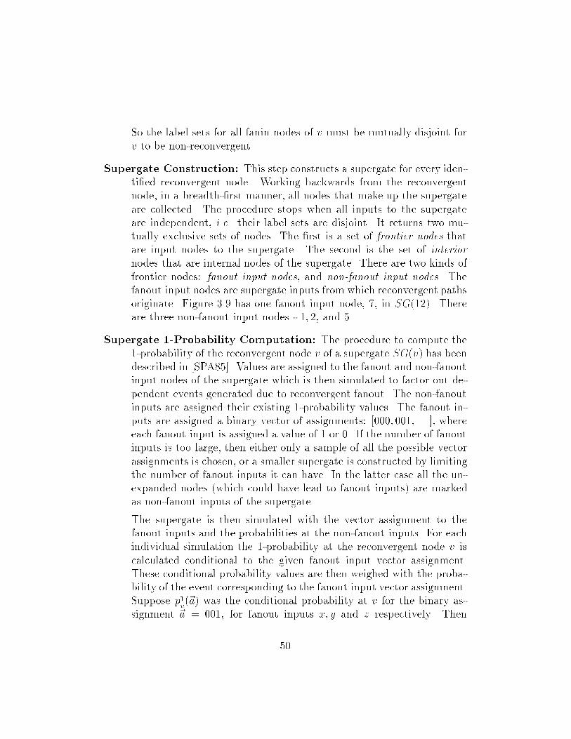
So the label sets for all fanin nodes of v must be mutually disjoint forv to be nonreconvergent�
Supergate Construction� This step constructs a supergate for every identi�ed reconvergent node� Working backwards from the reconvergentnode in a breadth�rst manner all nodes that make up the supergateare collected� The procedure stops when all inputs to the supergateare independent i�e� their label sets are disjoint� It returns two mutually exclusive sets of nodes� The �rst is a set of frontier nodes thatare input nodes to the supergate� The second is the set of interiornodes that are internal nodes of the supergate� There are two kinds offrontier nodes� fanout input nodes and non�fanout input nodes� Thefanout input nodes are supergate inputs from which reconvergent pathsoriginate� Figure ��� has one fanout input node � in SG����� Thereare three nonfanout input nodes �� �� and ��
Supergate ��Probability Computation� The procedure to compute the�probability of the reconvergent node v of a supergate SG�v� has beendescribed in �SPA���� Values are assigned to the fanout and nonfanoutinput nodes of the supergate which is then simulated to factor out dependent events generated due to reconvergent fanout� The nonfanoutinputs are assigned their existing �probability values� The fanout inputs are assigned a binary vector of assignments� ����� ���� � � �� whereeach fanout input is assigned a value of � or �� If the number of fanoutinputs is too large then either only a sample of all the possible vectorassignments is chosen or a smaller supergate is constructed by limitingthe number of fanout inputs it can have� In the latter case all the unexpanded nodes �which could have lead to fanout inputs� are markedas nonfanout inputs of the supergate�
The supergate is then simulated with the vector assignment to thefanout inputs and the probabilities at the nonfanout inputs� For eachindividual simulation the �probability at the reconvergent node v iscalculated conditional to the given fanout input vector assignment�These conditional probability values are then weighed with the probability of the event corresponding to the fanout input vector assignment�Suppose p�
v��a� was the conditional probability at v for the binary as
signment �a � ��� for fanout inputs x� y and z respectively� Then
��

p�v��a�� �p�
x�p�
y�p�
z� is the weighted conditional probability at the recon
vergent node for event ���� This weighted sum over all fanout inputassignments yields the exact �probability at the reconvergent node�
The tradeo� between computational e�ciency and probability accuracyarises when the fanout node set is too large� In such a situation whensimulating with the set of all possible fanout input assignments becomesimpractical a sample subset is used� Accordingly the �nal probabilityis also scaled by the size of this sample set�
Spatial Entropy Computation with Supergates�While removing errors in the spatial entropy at a reconvergent node the
steps of reconvergent node identi�cation and supergate construction outlinedabove do not change� But having constructed the supergate and computedthe �probability at the reconvergent node its spatial entropy and spatial entropy vector must also be calculated� Informally this task can be described asfollows� To start with the constructed supergate is treated as an independentcircuit� The existing spatial entropy S and spatial entropy vector �S values atits frontier nodes are saved� In Figure ���� this happens to nonfanout nodes�� � and �� and fanout node �� Since the frontier nodes of the supergate areprimary inputs of an independent circuit these are now initialized with a su
pergate spatial entropy Ssg and spatial entropy vector�Ssg� So Ssg
Ssg� S
sg��
and Ssg are initialized and the entropy vectors are initialized similarly� Then
the local spatial entropy ��Ssg� and spatial entropy vector ���Ssg� values for
the supergate are computed using the normal spatial entropy computationprocedure� At the end of this the supergate can be viewed as one large gatesimilar to the other �AND OR NAND� gates� Figure ���� shows this� Theselocal �supergate� spatial entropy and spatial entropy vector values are combined with the saved spatial entropy and spatial entropy vector values at thesupergate inputs to yield a cumulative expressions for the spatial entropy Svand spatial entropy vector �Sv at the reconvergent node� We now elaborateon these steps�The procedure to calculate the spatial entropy Ssg local to the supergate is
not as straight forward as the procedure to calculate the exact �probability�This is because the spatial entropy �and the spatial entropy vector� are aggregate concepts de�ned over a collection of input assignments or an entireprobability distribution� A node with an assigned value of � or � has a spatial
��

1
2
7
5
− Fanout Input Node
− Non Fanout Input Node
811
9
12Supergate SG(12)
Figure ����� The Supergate SG���� denoted as one Large Gate Node
��
entropy of � since its information content H is �� Hence the spatial entropyof the supergate cannot be calculated while simulating the supergate withbinary ����� values� It can be done only after the exact �probability iscomputed at the reconvergent node�The procedure to compute the spatial entropy at the reconvergent node
consists of the following steps�
�� Compute exact �probability of the reconvergent node�
�� Compute spatial entropy and spatial entropy vector local to the super
gate �Ssg and��
�Ssg�
�� Add these values to the spatial entropy and spatial entropy vectorvalues saved at the inputs of the supergate to obtain Sv and �Sv atthe reconvergent node�
We discuss each of these individually�
Step �� This step is identical to the supergate �probability calculation procedure discussed earlier�
Step �� Having computed the exact �probability at the reconvergent nodeanother pass is made through the supergate to compute the spatial
entropy �Ssg and spatial entropy vector���Ssg local to the supergate� For
this the fanout inputs of the supergate are �rst initialized to a spatialentropy of �� The nonfanout inputs are initialized to their local spatialentropy �H ��� which is computed from their �probabilities� Since thesupergate is being treated as an independent circuit the spatial entropyvector for the supergate has as many components as the number offrontier nodes in the supergate �fanout inputs � nonfanout inputs��As in the normal spatial entropy computation procedure the spatialentropy vector at a frontier node xi is initialized with a zero at allpositions except at position i�
Next a breadth�rst traversal of the nodes in the supergate is performed and spatial entropy and spatial entropy vector values are calculated at all the nodes inside the supergate to �nally obtain a value
for �Ssg and ���Ssg�
��

Step �� In this step the local spatial entropy and spatial entropy vector values at the supergate are combined with the existing spatial entropy andspatial entropy vector values at the supergate inputs to obtain the spatial entropy and spatial entropy vector at the reconvergent node� Weexpress this formally as follows� Suppose we have an ninput circuitwith a reconvergent node v whose supergate has m inputs and super
gate spatial entropy and spatial entropy vector values of �Ssg and ���Ssg�
The spatial entropy and spatial entropy vector of the reconvergent nodev can be expressed as follows
Sv �mXi��
Sxi � �Ssg �����
�Sv�
mXi��
��Sxi ��
��Ssg �����
where Sxi and�Sxi are the saved spatial entropy and spatial entropy
vector values at the frontier node xi of the supergate�
The vector��
Sxi is nelements long while ���
Ssg is m elements long sincethe former is in terms of the primary inputs of the circuit while thelatter is in terms of the inputs of the supergate� n and m can be
di�erent� So the values in ���Ssg have to be distributed proportionately
in terms of the primary inputs of the circuit� A supergate input xi willhave a saved spatial entropy and spatial entropy vector of Sxi and
�Sxi�
It will also have a contribution ���
Ssg�xi� in the local spatial entropyvector of the supergate� So if we distribute this contribution amongstthe primary inputs in the vector �Sxi we can obtain the local spatialentropy contribution for a given primary input j as
���
Sxi�j��
��
Sxi�j�
Sxi� �
��
Ssg�xi�
Since we have now expressed the supergate spatial entropy contributions in terms of the primary inputs we can write Equation ��� as
�Sv�
mXi��
���Sxi ��
��Sxi�
��

At the end of this third step the probability spatial entropy and spatialentropy vector at the reconvergent node have been calculated�
To summarize we have introduced the spatial entropy concept as a dynamic attribute in the circuit domain and de�ned it quantitatively using theentropy function in information theory� We explained how spatial entropycan provide a quantitative measure of the switching energy in a physicalcircuit implementation� A simple algorithm to estimate spatial entropy ingatelevel circuits was described� The spatial entropy attribute was extendedto describe spatial entropy vectors� Computing spatial entropy accurately isdi�cult� We discussed the various factors that a�ect the accuracy of its computation� The e�ects of minimization wire length and reconvergent fanoutare not necessarily independent� For instance minimization reduces literalcount but does not necessarily reduce wire lengths and hence spatial entropy�Since minimization can also alter the structure of reconvergence in a circuitthis too can a�ect spatial entropy� All this makes it all the more di�cultto characterize the e�ects of each factor independent of the other� In thenext chapter we discuss an application of spatial entropy to the problem ofvariable ordering for binary decision diagrams �BDDs�� This application alsohelps us evaluate the various approximations in computing spatial entropyand their e�ects on the solution�
��
Chapter �
Spatial Entropy Based BDD
Ordering
In this chapter we study an application of spatial entropy using it togenerate input variable ordering for binary decision diagrams�BDDs�� Theproblem of generating an ordering for the primary input variables of a booleanfunction in order to build small BDDs is an important one and has been studied extensively �MWBV�� FFK�� MIY�� Ber�� ISY�� JPHS�� BRM��MKR���� The ordering strategies in most of the literature rely on a staticexamination of the circuit topology� In this chapter we propose a dynamicapproach to generate variable orders that uses spatial entropy to capture theaggregate dynamic data movement in the circuit� We begin by introducingBDDs and motivating the variable ordering problem� After a short survey of
related research we outline our approach of using spatial entropy vectors��
S to generate variable orders� In Section ��� we describe the experimental setup to test our approach� After we state the objectives and assumptions wedescribe the data set the software and the experimental apparatus� Then inSection ��� we present our results followed by observations and conclusions�
��� Introduction and Motivation
In this section we begin with an introduction to binary decision diagrams andordered binary decision diagrams� Then we introduce the variable orderingproblem motivate it and summarize related research in this area�

����� Binary Decision Diagrams
A binary decision diagram �BDD� �Bry��� is a directed acyclic graph �DAG�representation �V�E� of a Boolean function f � I � f�� �g� The input variables I of the function are represented by nodes in the graph � The nodeset V of the graph contains two types of nodes� non�terminal nodes and ter�minal nodes� A nonterminal node corresponds to a boolean input variableand is labeled by the name of the variable� A terminal node corresponds tothe boolean constants � or � and is labeled T �true� or F �false� respectively�A fanout edge of a nonterminal node x � V is labeled with a � or �� Thislabel �� or �� denotes the value that is assigned to the boolean variable xalong this path� The fanout edge �x� y� � E leads from x to y where y iseither another nonterminal node or a terminal node� In the latter case y islabeled T or F � The node y is called the child of x �child�x� � y� and xis called the parent of y� The value of the function for a given assignmentto the input variables is determined by traversing the digraph �V�E� fromthe root down to a terminal node following a � or � edge depending uponthe value assigned to the boolean variable at that node� The value of thefunction equals � if the terminal node is T and � if the terminal node is F �Binary decision diagrams were �rst introduced in �Lee��� and further
popularized by Akers �Ake���� In �Bry��� Bryant introduced ordered binarydecision diagrams �OBDDs� a restriction on the class of binary decisiondiagrams� In an ordered BDD a strict ordering � is imposed on the inputvariables� The labeling of the nodes along any path from the root to theterminal node must follow the order given by �� This ordering can be formallyde�ned as follows� Suppose we are given a boolean function f with a set ofinput variables I where each variable in I is assigned an index according tothe ordering function � � I � f�� � � � � j I jg� A BDD for the function f underan ordering � has to satisfy the following constraint� Given nonterminalnodes w� x and y ��x� ��y� if and only if the following relation holds�
��child�x� � y�� ��x� ��y�� ���child�w� � y � ��x� ��w�� � ��x� ��y��
Figure ��� shows an example OBDD for the function a��b� � a��b� � a��b�with the ordering � � a� b� a� b� a� b�� Informally this ordering isspeci�ed by the sequence of variables in ascending order fa�� b�� a�� b�� a�� b�g�Since we are only interested in ordered binary decision diagrams the rest ofour discussion shall use the term BDDs to refer to ordered BDDs�
��

T F
01
1
T1
0
0
0
0
1
1 0
T
F
1
a1
a2
a3
b 3
b 1
b 2
Figure ���� OBDD of f � a��b� � a��b� � a��b� with orderingfa�� b�� a�� b�� a�� b�g
��

The variable ordering restriction on BDDs has several desirable propertiesfor symbolic boolean manipulation� In particular for a given variable ordering � the smallest BDD for a function is unique� Any BDD can be reducedto yield this unique representation by a simple e�cient algorithm �Bry����Furthermore many Boolean functions have e�cient polynomial size BDDrepresentations making it e�cient to manipulate such functions and performoperations on them� This in turn yields e�cient algorithms �Bry�� BBR���for tasks such as� determining if an input assignment satis�es a function�satis�ability testing� testing the equivalence of two functions �tautologychecking� and combining two functions with a boolean operation� Theseproperties led to the early use of BDDs in combinational logic veri�cation�Bry���� Since then they have been applied in several other areas of designautomation research� sequential veri�cation test pattern generation logicsynthesis and optimization� This is not surprising since the boolean function representation constitutes an important level of abstraction in the VLSIdesign process and an e�cient representation data structure bene�ts all thealgorithms employed at this level of abstraction�
����� The Variable Ordering Problem
A key issue that determines BDD size is the input variable ordering� TheBDD for a function can be very sensitive to the variable ordering� Figure ���shows a BDD of the function represented in Figure ��� but with a di�erent ordering � � fa�� a�� a�� b�� b�� b�g� The size of the BDD has increasedsubstantially�Bryant �Bry��� has shown that while for certain classes of Boolean
functions �integer multipliers� an e�cient �polynomial size� BDD representation does not exist regardless of variable ordering there are still alarge class of boolean functions that have e�cient BDD representations�The problem then becomes one of �nding a good input ordering thatwill yield an e�cient BDD representation� Since there are an exponential number �n#� of possible orderings for n input variables it is hardto exhaustively determine the smallest BDD for a given function� Thebest algorithm so far to arrive deterministically at an optimal orderingfor a function has a time complexity of O�n��n� �FS���� Several e�orts�Ber�� MWBV�� FFK�� MIY�� ISY�� JPHS�� MKR��� have been devoted to developing heuristics or approximate strategies for �nding a good
��

0 1
01
01
F
FT
0 1
0
0
1
T
01
0
10
1
01
FT
01
T
1
T0
01
TF
1
T
0
a 1
a2
a 3
a 2
a3 a3 a3
b1 b 1 b 1 b1
b 2 b 2
b 3
Figure ���� OBDD of f with ordering fa�� a�� a�� b�� b�� b�g
��

ordering to build small BDDs�There are two broad directions along which these heuristics to solve the
BDD ordering problem can be classi�ed� In the �rst category are the approaches �MWBV�� Ber�� MIY�� JPHS�� FFK�� BRM��� that relybroadly on the idea that an input node further away from the output has agreater in�uence on the BDD size than an input node closer to the output�These approaches perform a static analysis over the topology of a multilevel implementation of the function� They de�ne one or more attributes tocapture the depth of nodes in the static structure and then generate theorderings using these attribute�s�� For instance �MWBV��� uses node levelsand transitive fanin �TFI� depths as static attributes on a multilevel graphmodel of the implementation� The decreasing fanout count in the graph isused �FFK��� as a heuristic in an approach that generates orderings with theobjective of minimizing the number of crossings of a net� An observabilitybased approach is used in �MIY���� Other approaches use techniques basedon algebraic structure theory �JPHS��� and register allocation �Ber���� Allthese strategies typically require a breadth or a depth �rst traversal of thenetwork and can consequently generate orderings in a short time� But onthe other hand they do not seem to be able to generate consistently goodorderings� Butler et al� �BRM��� believe that a single algorithm might beinadequate for this purpose� so they use a suite of heuristics to solve theproblem�The second category consists of approaches that are more recent �FMK��
ISY�� MKR���� They formulate the ordering problem as an optimizationproblem� For a given ordering a cost function is de�ned to estimate BDDsizes� Then starting with an initial ordering and with the objective of minimizing the cost function optimization techniques like simulated annealingand variable exchanging within a window are used to generate improved orders� These techniques are more exhaustive and they spend a lot more timeexamining di�erent orderings before generating the best one� Thus theytrade computation time for a more thorough search of the space of variableorderings� Consequently they have yielded better BDD sizes than all theapproaches in the �rst category�In �PAS��� a slightly more fundamental approach is discussed where the
variable ordering strategy is part of the factorization process� Starting with atwolevel irredundant sum of primes form of the function a procedure calledlexicographic factorization is adopted� This procedure imposes a partial or
��
dering on the input variables of the function while generating the multilevelfactored form� The intuition behind using this factorization strategy is thatif excessive factorization can be controlled by controlling input dependencythen it yields a structured logic cone implementation that prevents the wiringcomplexity from increasing across di�erent cones in the implementation� Thepartial ordering of the input variables in the structured logic cone becomesthe variable order for the BDDs� This ordering is further optimized withvariable exchanging and then used to build the BDDs� We categorize thisapproach as more fundamental than the others because the variable ordersare generated while keeping in mind how the �n cubes of the function combine with each other during the factorization� The approach has encounteredproblems while generating orderings for the larger more complex benchmarkcircuit functions� This could possibly be due to the use of a greedy algorithmto generate the factors�Our approach is similar to the �rst set of techniques in that it requires an
existing circuit topology to �nd an ordering� But it di�ers from them in thatit uses a dynamic attribute spatial entropy as a discriminator for variableordering instead of a static circuit attribute� Such an attribute we believecan be related to a fundamental characteristic of the function� We elaborateon this in Chapter ��
����� Motivation
Why do we think that spatial entropy can help generate good variable orders�A BDD is a representation for a boolean logic function� Its size is in�uencedby some characteristics of the literals and the minterms of the function andnot by the implementation of the function� So when static attributes such asfanout depth or level �computed on an implementation of the function� areused to generate input variable orderings what characteristics of the literalsand the minterms are they trying to capture and how do they use the implementation of the function for this purpose� The number of onterms andthe spatial distribution of these onterms in the cube space of the functionwill in�uence the implementation of the function� The spatial distributionin�uences the degree to which the onterms can be combined to yield largercubes� For instance in the multilevel �factored form� implementation off � a�b� dc�e� h�g�� � bi the literal a belongs to several onterms not all ofwhich can be combined� Hence it typically appears at the outermost position
��

in the factored form representation of the function� In contrast the few onterms that literal g belongs to can be combined easily and it is nested deepinside the factored form� Since a factored form closely resembles a multilevelimplementation of the function the level or depth of nodes helps serve as adiscriminator between input literals� So the depth or level of the nodes inthe implementation is actually capturing some characteristic of the literalsand minterms of the function that in�uence the BDD size� But the precisemanner in which these literals and minterms in�uence the BDD size is stillnot clear� Hence this approach acts as a heuristic�Ordering variables on static depth or distance �from the output� may
not always help� This is because while the distance or depth measure ina static attribute may provide some information to discriminate betweenliterals in a minterm it may not capture su�cient information about how allthe �n minterms of a given function combine with each other� Furthermorewhen implementations fail to provide clear depth information it makes itmore di�cult to use static depth to discriminate between literals in di�erentminterms� This is seen in a parallelpre�x adder where the least signi�cantinput bit that in�uences the maximum number of onterms is at the samestatic distance O�log n� from the output as the most signi�cant input bit�The spatial entropy attribute tries to capture the spatial distribution of
the minterms in the cube space of the function� Like the other static attributes it too is computed on an implementation of the boolean function�The attribute has two components� It relies on the entropy function Hw forinformation about the �n minterms of a function� Hw is probability based andit provides dynamic usage information that helps determine the in�uence ofindividual literals on the minterms� It relies on the distance attribute l�w�w��to capture the spatial distribution of these minterms in the cube space� Whenminterms �or cubes� are too far apart in cube space they cannot be combinedto create larger cubes� The literals that make up these minterms cubes alsocannot be shared� As a result implementations of these minterms cubes thatare spatially apart in cube space will require wires or fanouts to bring themtogether in order to combine them� We also notice that in an implementation wires are needed to bring together blocks of unevenly sized logic�This will also happen when unevenly sized cubes have to be combined� Ifthe cubes themselves cannot be shared then wires would be needed in theimplementation to stretch the output of the larger cube!s implementationto combine it with the smaller cube� This issue and other issues related to
��

function complexity are treated in further detail in Chapter ��Spatial entropy is attempting to capture the spatial distances that the
cubes and minterms have to travel using its l�w�w�� attribute� By combiningusage with Hw and distances with l�w�w�� the spatial entropy attribute is computing dynamic distances of the input nodes over all possible minterms� Thiswe feel will yield a stronger discriminatory measure than static depth� Forinstance consider the addition function� Two static attributes depth andarea of di�erent implementations �carryripple carryskip carryselect andparallelpre�x� of an adder have a broad range of values� On the other handthe dynamic information about these circuits such as average case delays tothe output nodes have a smaller variance �Tya��b�� This indicates that anattribute like spatial entropy that captures both the static structure and dynamic usage may have lesser possible variations for di�erent implementationsof the same function� Hence it might be a better discriminator for variableordering than a static circuit attribute� In the next section we describe ourapproach of using spatial entropy to generate variable orderings�
��� Variable Ordering using Spatial Entropy
In Chapter � we described a procedure to compute the spatial entropy atthe output nodes of a combinational logic function� Then in Section �����we extended this procedure by characterizing the total spatial entropy ofthe circuit in terms of spatial entropy contributions of the primary inputs�This was done by adding an attribute called spatial entropy vector �S toevery node in the network� For a circuit with n primary inputs the spatial
entropy vector at any node w�Sw is an nelement vector that re�ects the
contribution of each primary input to the spatial entropy value at node w�The spatial entropy at the node w is the cumulative sum of the spatial entropycontributions of each primary input�
Sw �nX
j��
�
Sw �xj�
In the case of primary inputs the spatial entropy vector at each input xj�Sxj consists of �s at all input positions except for position j which containsa �� This indicates that the spatial entropy at this node is � which is entirelycontributed by the primary input xj�
��

The spatial entropy vector at an internal node w is computed by distributing the local spatial entropy computed at the node amongst the primary inputs in the support set of every fanin of node w� For a node w withk fanins w�� w�� � � � � wk the spatial entropy contribution of primary inputxj at node w can be expressed as�
��
Sw�xj����
Sinw�xj� ��SwSinw
���
Sinw�xj�
where �Sw is the local spatial entropy at node w��Sinw �xj� is the total
spatial entropy contribution of primary input xj at the fanins of node w and
Sinw �Pn
j��
��Sinw �xj� i�e� the total spatial entropy over all the fanins of
node w� This expression was discussed in detail in Section ������In order to generate an ordering for the primary inputs of a function using
the spatial entropy vector ��S � at the output nodes let us review the examplein Section ������ The �gure is reproduced in Figure ��� for easy reference� Thecircuit has a single output node n��� The spatial entropy at this node is S ������� This is expressed as the spatial entropy contribution of primary inputsi�� � � � � i� in the spatial entropy vector at n�� � ��������������������������
It may be recalled from Chapter � that spatial entropy was de�ned asthe total information �ow through the function giving us a measure of the
e�ort required to compute the function� The spatial entropy vector�S at
an output node contains the spatial entropy contributions of the primaryinputs �at that node�� This gives a measure of the e�ort required to computethe output function in terms of the primary input contributions� So fromthe vector ������������������������we �nd that inputs i�� i� contributeequal amounts to the spatial entropy at n�� i� contributes the most and i�contributes the least�All our ordering strategies are based on the following premise� A primary
input that contributes less e�ort or spatial entropy towards the output func�tion is less likely to in�uence the size of the BDD for the function� Likewisean input that contributes the most e�ort or spatial entropy is most likelyto in�uence the size of the BDD� A node that appears earlier in the orderingfor a BDD has a greater in�uence on the size of the BDD� Hence an inputwith the highest spatial entropy contribution is given the highest position inthe input order� Similarly an input that has less spatial entropy contribution
��
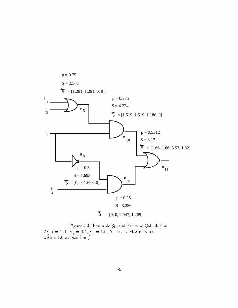
i
i
i
1
n
n
n
n
2
3
i4
5
S
8
9
n10
11
S = [1.281, 1.281, 0, 0 ]
S = 2.562
p = 0.75
p = 0.375
S = 4.224
S = [1.519, 1.519, 1.186, 0]
p = 0.5
S = 1.693
S = [0, 0, 1.693, 0]
p = 0.25
S= 3.256
S = [0, 0, 2.047, 1.209]
p = 0.5312
S = 8.17
= [1.66, 1.66, 3.53, 1.32]
Figure ���� Example Spatial Entropy Calculation ij j � �� � pij � ���� Sij � ��� �Sij is a vector of zeroswith a ��� at position j
��

will appear lower down in the orderings� In Chapter � we develop a strongerbasis for this premise�For a single output function we can generate variable orderings by order
ing the primary inputs in descending order of their spatial entropy contribu
tions in the spatial entropy vector�
S at the output node� But how does onegenerate variable orderings in a multioutput function� Consider a functionwith n inputs and m outputs� The e�ort contributed by primary input xi incomputing a given output function oj is expressed by the spatial entropy
vector at that output node�
Soj �xi�� So in order to determine the e�ort contributed by primary input xi in computing all the m output functions the
m output spatial entropy vectors�Soj �j � ��m� need to be combined� There
are several ways in which this can be done� We have tested three approachesthat we describe below�
Maximum� This approach is based on the intuition that an output with thehighest spatial entropy will have maximum say in the variable orderingprocess� This is because the logic cone for the output node �with highspatial entropy� is contributing the maximum percentage of the totalinformation �ow over all the output functions� Hence the variable ordering required to build a BDD for this output function should havethe maximum in�uence on the variable ordering required to build theBDD for all the output functions� Consider Figure ��� which illustratesan �input �output function with the distribution of spatial entropyvalues at each output� The spatial entropy or total information �owfor the �output function is the cumulative sum of the spatial entropiesof each output function� Since o� has the maximum contribution tothis total information �ow the spatial entropy vector associated withit should have the maximum in�uence on the ordering� This approachhas also been used by some of the static attribute based heuristics togenerate variable orderings� the di�erence is that instead of a dynamicattribute like spatial entropy static depths and levels of the nodes inthe logic cone were used�
The details of this strategy are as follows� First the primary output ojwith maximum spatial entropy �Soj � is considered� The input variablesare ordered in descending order of their spatial entropy contributions
��

o1
o
o
i
i
i
i
i
i
i
i
2
3
1
2
3
4
5
6
7
8
Figure ���� Spatial Entropy Distribution for a �output function �Maximum�
at oj using the spatial entropy vector �Soj � So
x� y � I x y iff�
Soj �x���
Soj �y� �����
In the above example the spatial entropy vector at output o� is ex
amined �rst� This vector�So� will not order input variables that have
equal spatial entropy contribution or zero spatial entropy contribution�The latter can happen when the input variables are not in oj!s supportset as is seen with i� i in the above �gure� As a result the aboveordering is really a partial ordering that partitions the input variableset I into a set Eoj of ordered disjoint equivalence classes� For output
oj Eoj � f�ji� � �ji� � � � �jilg l � n where each �jik consists ofeither a single input variable or a set of input variables such that
x� y � �jik
�
Soj �x���
Soj �y�
and
x � �jik � y � �jik� �Soj �x� � Soj �y�� � ��jik �jik� �
These classes �jik � Eoj are then re�ned by consulting the spatialentropy vector of the output with the nexthighest spatial entropy� In
��

i 1
i 2
i 8
i 7
i6
i5
i3
i 4
o2
o1
o 3
Figure ���� Spatial Entropy Distribution for a �output function �WeightedMultiply�
Figure ����So� is consulted and the ordering criteria in Equation ��� is
used to generate a re�ned set of equivalence classes Eo� � This process
continues until either all the input variables are ordered i�e j �jik j��� �jik � Eoj or the spatial entropy vectors of all the output nodeshave been examined� In the latter case if the input variables stillappear together in an equivalence class �j �ik j� �� then this indicatesthat the relative order of the elements in �ik is not important�
Weighted Multiply� In the previous approach we generated orderings bygiving maximum importance to the spatial entropy contributions ofone output� This was the output with the maximum spatial entropy�The �nal ordering is thus very largely determined by this output function and its logic cone� But not all functions exhibit this scenario�For instance in some multioutput functions an input that contributesheavily to one output may contribute very sparingly to all the otheroutputs� Consider Figure ���� Suppose in the cone of output o� thespatial entropy contribution of input i� is greater than that of i i�e�
�
So��i����
So��i�� We notice that while i� does not contribute to any otheroutput function i contributes to output functions o� and o� also� Insuch a situation with respect to the multioutput function as a wholeinput i could be contributing greater cumulative e�ort than input i��
��

Hence a more global variable ordering strategy is needed�
While the spatial entropy vector at the output node with the highestspatial entropy must have a high in�uence on the �nal variable orderings the spatial entropy vectors from the other outputs must also beable to in�uence the orderings� To do this for a given output oj every
element in the spatial entropy vector�
Soj �xi� is weighted by multiplying it by the proportion of the spatial entropy that its output node
oj contributes to the total circuit spatial entropySojPSoj� Then the
weighted spatial entropy vectors for all the outputs are added �in vec
tor form� to obtain one single cumulative spatial entropy vector �S��The contribution of input xi in this vector is given by
��
S��xi� �mXj��
���
Soj �xi� �SojPmk��
Sok
�
This strategy thus weighs the spatial entropy vector at each output interms of the percentage contribution of that output!s spatial entropyto the total circuit spatial entropy and then accumulates the weightedvectors� The descending order of the contributions in this weightedvector determines the order of primary input variables for the BDD�
Weighted Divide� This strategy is similar to the weighted multiply exceptfor the fact that instead of multiplying the elements of the spatial entropy vector by the output spatial entropy we divide them by the output spatial entropy� Dividing each spatial entropy vector by its outputspatial entropy normalizes all the spatial entropy vector contributionsto the ��� �� range� This suppresses the amount of in�uence that eachoutput spatial entropy value can exert due to its magnitude since allthe weighted vectors have a maximum value of �� Thus it treats everyoutput spatial entropy vector with equal importance� The e�ect of thisis that a primary input that contributes a consistently high percentageto all the outputs of a multioutput function may appear higher in theordering than an input that contributes a very high percentage to oneoutput and negligible amounts to others� For example given a pair ofinputs where input i contributes a spatial entropy percentage of ���� ���and ��� towards output functions o�� o� and o� respectively and input
��

j contributes a spatial entropy of ���� ��� and ��� respectively the inputj gets chosen as being more important ���� � �����
In the next section we describe our experiment to study the use of spatialentropy vectors to generate variable orderings for BDDs�
��� Experiment� Objectives and Criteria
The primary objective of this experiment is to study the e�ectiveness ofspatial entropy in generating good variable orders for BDDs� The criteriafor good variable orders is determined by the size of the resultant BDD thesmaller the BDD size the better the ordering� We compare the BDD sizesgenerated by the spatial entropy approach with those generated by otherheuristics �Bra�� BRM�� ISY�� MKR�� PAS���� The accuracy of thespatial entropy attribute as de�ned in Chapter � is a�ected by factors suchas logic minimization wire length and reconvergent fanout� The study of thee�ect of some of these factors on variable orderings is another objective ofthis experiment� Finally we also study the di�erent strategies that combinespatial entropy vectors� The results from this experiment will help evaluatethe e�ectiveness of this attribute in generating good variable orders� Inaddition it will help characterize how the inaccuracies in computing thisattribute a�ect variable orderings� We also hope that a study of the factorsa�ecting spatial entropy will provide us with a better characterization of thespatial entropy attribute to assist its application in other areas� We begin bydiscussing our assumptions and limitations after which we describe the dataset used for the experiment�
����� Assumptions and Limitations
Our �rst assumption is with respect to logic minimization� Computing thespatial entropy and the spatial entropy vector at the output nodes of a function requires an implementation� An unminimized implementation can a�ectthe spatial entropy � Figure ��� shows how the spatial entropy can increase�The implementation that is not minimized will have a greater spatial entropydue to the excess spatial entropy contribution from the additional gate� Evenlegitimate reasons for introducing redundancy like delay reduction are not
��

S =2.562
S=4.223 S =2.562
f = a+a’c f = a+c
a’
c
a
a
cS=1.0
Figure ���� Two implementations of the same function with di�ering SpatialEntropy
desirable in this particular case since it arti�cially increases the spatial entropy of some nodes over others� Hence we require our circuits to be minimalin literal count before performing spatial entropy computation� In practicesince minimization is a heuristic we only have approximately minimal circuits� Minimizing the circuit by removing redundant literals will help reducethe spatial entropy but the relationship between spatial entropy and logicminimization is not entirely straightforward� In larger complex functions therole of wire lengths becomes signi�cant� Let us see how�Given a twolevel or a multilevel representation of a logic function it
can be minimized �for literal count� using logicminimizers like espresso
�BHMSV��� along with one of the minimization scripts in the UC BerkeleyMISII SIS �Sequential Interactive System� system �BRSVW���� But sinceexact multilevel logic minimization requires exponential time �Law��� mostminimizers use heuristics to �nd �nearoptimal� solutions� The optimality ofsuch a solution is usually measured with respect to the minimal literal countin the multilevel implementation� The number of literals in�uences thenumber of nodes in the implementation� Since spatial entropy is computedover all the nodes in the implementation it is a function of this literal countmeasure�But minimizing literal count does not necessarily imply that the excess
spatial entropy �due to logic that is not minimized� is being removed� This isbecause wire lengths in the layout of such an implementation can reverse thise�ect� Figure ��� illustrates this in a very simpli�ed form� Version � factors
��

out the expression c�d and uses an extra fanout with a long wire to achievethe function� In contrast Version � avoids the factoring and replicates thegate implementing c � d� In the process it saves on the long wire� Whilethe redundant logic will contribute to the spatial entropy in Version � itsabsence in Version � is o�set by the long wire� This makes it di�cult toevaluate the e�ectiveness of the multilevel logic minimizers and minimizationscripts in completely solving the problem of generating implementations withminimum spatial entropy� With this scenario we assume for the present thatminimizing literal count does remove excess spatial entropy and we adoptthe minimization script that does the best job in minimizing the literal countwherever possible�Our next assumption deals with reconvergent fanout� In Chapter � we
had characterized the e�ect of reconvergent fanout on spatial entropy andoutlined approaches to remove errors in spatial entropy due to reconvergentfanout� Almost all VLSI circuits are reconvergent� Removing errors in spatialentropy values in such circuits is an exponential time procedure� Hence formost of the data in our experiments we elect to compute spatial entropy byignoring the e�ect of errors due to reconvergent fanout�Finally we discuss wire lengths� The e�ects of wire length on spatial en
tropy were described earlier in Chapter �� We had �rst discussed inaccuraciesdue to the absence of wire lengths and then followed it by discussing inaccuracies in the distribution of the lumped wire length along multiplefanoutnodes� What role do wire lengths play in variable ordering� In Section �����we had conjectured that the length attribute in the spatial entropy de�nitioncaptures the spatial distance that cubes and sets of cubes have to travel inthe implementation while computing the function� This distance is re�ectedin the implementation by wires that connect one set of gates �cubes� with another� One way of computing this wire length is to extract lengths from theschematic of a gate level netlist� But schematic generation for large netlistsis nontrivial and such tools are not easily available� The problem of gateplacement and interconnection in a netlist schematic has similarities with theplacement of cells in a layout synthesis system� We had access to a standardcell place and route system called VPNR �vanilla placeandroute� as part ofthe MCNC OASIS Silicon Compiler �KB���� So we decided to use layoutsfrom VPNR to extract our wire length estimates� This decision needs somejusti�cation�A netlist at the gate level can be realized at the layout level by a large set
��

c d
e a b
c d
Version 1 Version 2
c d
e a bf g f g
Figure ���� The tradeo� between redundancy and wire length
��

LAdmissable Set A
Layouts
CgGate level circuit
Figure ���� Mapping of Gate Level Circuits at the Layout Level
of layouts� All the layouts in this set will be functionally the same as the gatelevel implementation and will have the same set of nodes and gates� But thephysical layouts will di�er in other characteristics� The layout styles usedto realize the gates �standard cell full custom gate array� may be di�erent�The layouts may di�er in the total area the placement and routing betweenthe cells the number of layers in which routing is done the number of wiresand the the length of these wires� These di�erences arise due to the di�erentlayout methodologies and styles available and the di�erent criteria that theyuse while realizing the layout �minimize total area total wire length totalnumber of vias etc��� We are only interested in a subset of the set of allfeasible layouts called the admissible set A� This is the set of layouts thatyield a placement and interconnection pattern that is similar to our idealschematic placement� Figure ��� captures this scenario� The experimentproposes to use the wire lengths extracted from one such admissible layoutL � A of the gate level circuit Cg�We also assume that the wire lengths of internal nodes in a layout cor
��

relate well with those in a gatelevel schematic� By this we mean that forlayouts L�� L� � A lL�
w� lL�
v� lL�
w� lL�
v where lL�
wis the length of wire
w in layout L�� It is this relative ordering that we wish to capture� This isalso argued with some empirical evidence� In �RT��� the VPNR placeandroute system was used to generate layouts for regular data path functions likeadders and shifters� It was shown �with statistical regression analysis � thatVPNR generated layouts were a good �t to the expected analytical area ofthese functions� The coe�cient of variance between the analytical curve andthe area plots was within �� for most cases� Since area is a function of wirelength this correlation ought to hold with respect to wire lengths too� Thiscorrelation can be generalized to randomlogic circuits because the VPNRplaceandroute system performs its placement and generates its wires without any knowledge of the circuit function� Hence its behavior should notbe expected to change with circuit function� It must be emphasized herethat extracted wire lengths from a layout are not necessary for this experiment� They just happen to be a convenient source for obtaining wire lengthestimates between gates in a circuit�The next assumption we make is with respect to the process of wire length
extraction itself� The layout synthesis system and the extraction softwareforce us to make approximations� While the errors due to these approximations will not give us the exact wire length in the layout our hope is thatthey are small enough not to a�ect the relative wire length distribution�The �rst approximation is with respect to point�to�point versus lumped
wire lengths� Since we are primarily interested in interconnect length we wishto obtain length estimates for only the wires used in the routing between cellsin a layout� Wire lengths of layers inside a standard cell �gate� are not ofinterest to us� For a node that fans out to several other nodes ideally we wishto obtain point�to�point interconnect lengths for each individual fanout wire�This is di�cult to do because of two reasons� Firstly multipoint nets in alayout are usually routed using a minimal Steiner tree that inserts additionalpoints in the route that do not belong to the net� This makes pointtopointestimates di�cult� This also makes it di�cult for the the extraction softwareto extract wire lengths between nodes or points on a net� As a result wesubstitute pointtopoint lengths by estimates of total lumped wire length ata node�Our second approximation is with respect to the layers that constitute the
lumped wire length estimate� The extraction software extracts area and not
��

wire length� Dividing this area estimate by a constant factor should give uslength information since most rectangles in the layout have a fairly uniformwidth ������ The extractor generates the area of the rectangles by extractingthe areas of all the di�erent layers at a given node� This includes contacts�metal�� metal� poly� �n and p diff etc�� Assuming we can suppressarea extraction inside a cell we would still be including areas of severalcontacts in the intercell routing� We assume that retaining these areas alongwith the areas of the layers actually used for routing will not perturb the wirelength estimate enormously� To summarize our three main assumptions are
� We assume that aggressive literal count minimization helps reduce excess spatial entropy in redundant circuits�
� Reconvergent fanout removal is ignored�� An estimate of the pointtopoint interconnect wire length in a gatelevel netlist is obtained by using the lumped area of all intercell layers electrically connected at a given node in a �VPNR� layout of thatnetlist�
The primary limitation of our experimental set up is that it is di�cult toevaluate the magnitude of our approximations in spatial entropy computation� The only way to determine if an approximation in the spatial entropycomputation is good or bad is by generating variable orders building BDDsizes and comparing them� The fact that many approximations assumptions�like redundancy and wire length� are interdependent also makes it di�cult to isolate an approximation and characterize it separately� Two otherlimitations are the di�culty of computing exact spatial entropies in highlyreconvergent circuits with large supergates and the lack of more precisepointtopoint wire lengths between nodes� The e�ect of redundancy on spatial entropy is also not very clear� The spatial entropy is a function of wirelengths� Although the e�ect of di�erent minimization scripts on wiring areawas documented in �Sau��� it is is not clear how the use of minimizationscripts to remove redundancies will a�ect the wire length and what e�ectthat has on spatial entropy�
��

����� Data Set
The requirements of the data set for this experiment are as follows� Firstlythe data set should consist of benchmark circuits that can be used to compare the performance of the spatial entropy based BDD ordering with otherapproaches� The data set should also contain circuits that represent regularstructured logic and random combinational logic to evaluate BDD sizes inthese two domains� Finally it must contain small and large circuits� smallcircuits where the e�ects of the factors a�ecting spatial entropy can be studied more closely and large circuits to ensure that orderings for nontrivialcircuit examples can also be obtained�To satisfy these requirements our data set consists of three classes of
circuits� In all three classes we use the MCNC VPNR format �KB��� torepresent the multilevel netlist as input to the spatial entropy computationprocedure spent� The VPNR format is a circuit description format thatdescribes a technology mapped netlist in terms of the standard cells in theMCNC standard cell library�
ISCAS� Circuits� This data set consists of multilevel circuits from theISCAS �� benchmarks� There are several large circuits here which canhave signi�cantly di�ering BDD sizes highlighting good and bad orderings� The circuits have wellde�ned characteristics number of nodesnumber of inputs number of outputs� There is also a mix of circuitfunctions adder priority encoder random logic ALUs etc�� Thesecircuits have also been used as the primary data set for comparing various BDD ordering strategies for combinational circuits� We use theUC Berkeley MISII SIS system �BRSVW��� to further minimize thesecircuits and then translate them into the VPNR format� Table ���illustrates some characteristics of these circuits�
LgSynth� Circuits� These are benchmark circuits compiled at theMCNC Logic Synthesis Workshop �in May ������ These circuits arein twolevel and multilevel form� The circuits are a lot smaller thanthe ISCAS�� circuits giving us an opportunity to study the e�ects offactors a�ecting spatial entropy� They have also been used to compareBDD ordering strategies� They too consist of a mix of random andstructured logic� The �level form of the circuits gives us an opportunity to study the e�ect of the di�erent minimization scripts in SIS on
��

Circuit Circuit TotalName Function Inputs Outputs Gates
C��� Priority Decoder �� � ���
C���� ECAT� �� �� ���
C��� ALU and Control �� �� ���
C����� ECAT �� �� ���
C���� ECAT �� �� ���
C���� ALU and Control �� �� ����
Table ���� ISCAS �� Benchmark Circuit Characteristics�ECAT stands for Error Correcting and Transmission��Circuits C��� and C���� are functionally equivalent�
spatial entropy computation and variable ordering� The �nal netlistform is obtained by using SIS to minimize the circuit and then translating it to the VPNR format� The circuit characteristics are describedin Table ��� and Table ���� The functions of the twolevel circuits areunknown�
OASIS Generated Circuits� These are circuits generated using the OASIS silicon compiler tool set �KB���� They are primarily circuit descriptions of regular structured circuits in various sizes� This includes adders decoders encoders multiplexors multipliers shiftersand counters with bit widths varying from � to ���� The circuits weredescribed in LOGICIII and OASIS was used to generated the VPNRgatelevel netlist� The multilevel minimization strategy used here wasMCNC!s DECAF �LKB��� and not the Berkeley SIS scripts� This isbecause DECAF is part of the OASIS system� This data set helpscharacterize the behavior of the spatial entropy procedure on regularstructured circuits� Their characteristics are described in Table ����
��
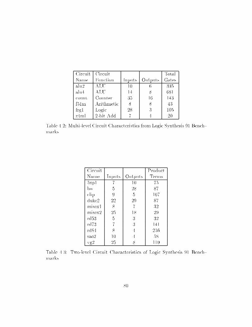
Circuit Circuit TotalName Function Inputs Outputs Gatesalu� ALU �� � ���alu� ALU �� � ���count Counter �� �� ���f��m Arithmetic � � ��frg� Logic �� � ���z�ml �bit Add � � ��
Table ���� Multilevel Circuit Characteristics from Logic Synthesis �� Benchmarks
Circuit ProductName Inputs Outputs Terms�xp� � �� ��bw � �� ��clip � � ���duke� �� �� ��misex� � � ��misex� �� �� ��rd�� � � ��rd�� � � ���rd�� � � ���sao� �� � ��vg� �� � ���
Table ���� Twolevel Circuit Characteristics of Logic Synthesis �� Benchmarks
��
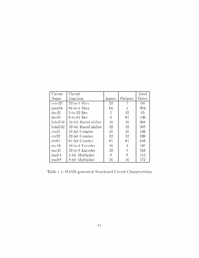
Circuit Circuit TotalName Function Inputs Outputs Gatesmux�� ��to� Mux �� � ���mux�� ��to� Mux �� � ���dec�� �to�� Dec � �� ��dec�� �to�� Dec � �� ���bshift�� ��bit Barrel shifter �� �� ���bshift�� ��bit Barrel shifter �� �� ���ctr�� ��bit Counter �� �� ���ctr�� ��bit Counter �� �� ���ctr�� ��bit Counter �� �� ���enc�� ��to� Encoder �� � ���enc�� ��to� Encoder �� � ���mult� �bit Multiplier � � ���mult� �bit Multiplier �� �� ���
Table ���� OASIS generated Structured Circuit Characteristics
��

To summarize the data set consists of about �� example circuits morethan � �rds of which are benchmark circuits� The remainder are structuredcircuits generated by OASIS that exhibit a more regular communicationbehavior� The circuits vary widely in size� The inputs range from � to ��and the outputs range from � to ��� This yields a wide range of possible BDDsizes from � to ��� in the worstcase� The circuit sizes range from �� gates toapproximately ���� gates� The circuit function is also well distributed� Thereare datapath structures like ALUs shifters counters multipliers etc�� buslike structures for select transmitting and encoding data like multiplexorsdecoders and encoders� Finally there is random glue logic of varying size�
��� Experiment Outline
Our objectives are threefold� Firstly we would like to see how the spatialentropy attribute performs in generating variable orders for BDDs� For thiswe compare it with the other approaches� those based on static attributesand those based on optimization techniques� Secondly we would like to analyze the e�ect of some of the factors a�ecting spatial entropy by computingspatial entropy with di�erent approximations� Finally we would like to compare the various strategies of combining the output spatial entropy vectorsin multioutput functions� All these goals require the generation of BDDsusing the spatial entropy approach� The experimental set up described inFigure ��� shows how this is done� The oval boxes indicate software whilethe rectangular boxes indicate data� The orderings generated by the spatialentropy computation procedure spent are fed to a BDD builder vpnr�bddto generate BDD sizes� The orderings that we wish to compare with are alsobuilt using the same BDD builder� This is done in order to remove implementation dependent discrepancies in BDD sizes of the di�erent approaches� Wenow describe the software construction for the experiment and then outlinethe variables measured�
����� Software Construction and Variables Measured
As Figure ��� indicates the experiment required � pieces of software� Thespatial entropy computation program spent was written to accept the inputcircuit description compute the spatial entropy and spatial entropy vector for
��

Variable Orderings
vpnr2bdd
Other OrderingsOther Orderings
from Spent
spent
len_extract
Input Data Set
Choose Ordering
Input Data Set
BDD Size
Wire Length
Figure ���� Experimental Setup
��

the nodes in the circuit and generate variable orders for the primary inputsof the circuit using the di�erent strategies discussed in Section ���� In orderto incorporate wire length information during spatial entropy computationwire lengths were extracted by len extract and then fed to spent� Finally aprogram called vpnr�bdd was employed �Ree��� to build BDDs for the inputcircuit descriptions in VPNR using either the generated variable orderingsfrom spent or orderings contributed from other sources�The criteria used to measure performance in this experiment was the size
of the built BDD� Hence it was the main variable measured for the di�erentcircuits in the data sets�
��� Results and Observations
We present our results in three phases along the lines of the three objectivesof the experiment� In the �rst phase we compare spatial entropy based BDDordering with static attribute based approaches and optimizationintensivestrategies� The same BDD builder vpnr�bdd was used to build BDDs forall the orderings� The BDD sizes are expressed as number of nodes� Inthe second phase we present results that illustrate the e�ects of some ofthe approximations redundancy wire length and reconvergent fanout onBDD sizes� Results for all the � data sets are discussed here� Finally wepresent results comparing the three di�erent strategies of combining spatialentropy vectors of multioutput functions to generate variable orders� All theexperiments were run on a DECStation ���� ��� MB� running Ultrix Version���A�
����� Spatial Entropy and BDD Sizes
We illustrate our results with respect to two data sets� Table ��� comparesBDD sizes generated by spent for the MCNC Logic Synthesis �� benchmarkcircuits with � other sources� These sources were chosen because they arerepresentative of related approaches to BDD variable ordering� They werealso the only sources known to us that had generated orderings for this setof benchmarks� Finally these ordering sources are very recent giving us anopportunity to compare spent with the latest results�
��
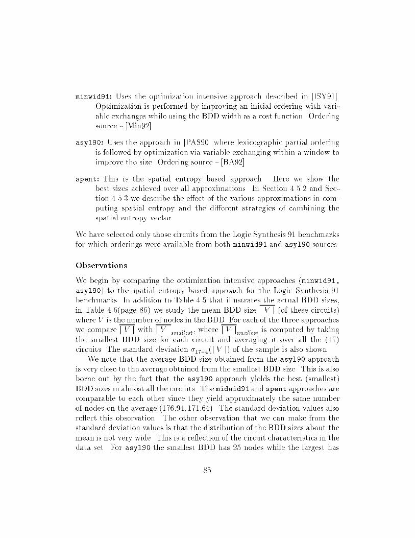
minwid��� Uses the optimization intensive approach described in �ISY����Optimization is performed by improving an initial ordering with variable exchanges while using the BDD width as a cost function� Orderingsource �Min����
asyl��� Uses the approach in �PAS��� where lexicographic partial orderingis followed by optimization via variable exchanging within a window toimprove the size� Ordering source �BA����
spent� This is the spatial entropy based approach� Here we show thebest sizes achieved over all approximations� In Section ����� and Section ����� we describe the e�ect of the various approximations in computing spatial entropy and the di�erent strategies of combining thespatial entropy vector �
We have selected only those circuits from the Logic Synthesis �� benchmarksfor which orderings were available from both minwid�� and asyl�� sources�
Observations
We begin by comparing the optimization intensive approaches �minwid���asyl��� to the spatial entropy based approach for the Logic Synthesis ��benchmarks� In addition to Table ��� that illustrates the actual BDD sizesin Table ����page ��� we study the mean BDD size j V j �of these circuits�where V is the number of nodes in the BDD� For each of the three approacheswe compare j V j with j V jsmallest where j V jsmallest is computed by takingthe smallest BDD size for each circuit and averaging it over all the ����circuits� The standard deviation �����j V j� of the sample is also shown�We note that the average BDD size obtained from the asyl�� approach
is very close to the average obtained from the smallest BDD size� This is alsoborne out by the fact that the asyl�� approach yields the best �smallest�BDD sizes in almost all the circuits� The midwid�� and spent approaches arecomparable to each other since they yield approximately the same numberof nodes on the average �������� �������� The standard deviation values alsore�ect this observation� The other observation that we can make from thestandard deviation values is that the distribution of the BDD sizes about themean is not very wide� This is a re�ection of the circuit characteristics in thedata set� For asyl�� the smallest BDD has �� nodes while the largest has
��

Circuit $ of NodesName minwid�� asyl�� spent
alu� ��� ��� ���alu� ���� ��� ���count ��� ��� ���f��m �� �� ��frg� ��� �� ���z�ml �� �� ���xp� �� �� ��bw ��� �� ���clip ��� ��� ���duke� ��� ��� ���misex� �� �� ��misex� ��� �� ���rd�� �� �� ��rd�� �� �� ��rd�� �� �� ��sao� �� �� ���vg� ��� �� ���
Table ���� Comparative BDD sizes for Logic Synthesis �� Benchmarks
Mean and Standard Deviation of BDD sizesStatistic minwid�� asyl�� spent smallest
jV j������ ������ ������ ������
����j V j� ������ ������ ������ ������
Table ���� Comparative Statistics for Logic Synthesis �� Benchmarks
��

��� nodes� In fact if alu� is excluded then the range of BDD sizes dropsfurther ���� �����While the asyl�� approach de�nitely has the best performance for this
data set we would now like to see how the spent and minwid�� approachescompare with it� Table ����page ��� shows the normalized BDD sizes forthe spent and minwid�� approaches computed as a fraction of the sizesgenerated using asyl��� To analyze this better we compare average performance and standard deviation of these approaches with respect to that ofasyl��� Since the BDD sizes are normalized with respect to asyl�� sizeswe are comparing against a mean of ��� and a standard deviation of ����The minwid�� approach has an average normalized BDD size of ���� whilespent has an average normalized BDD size of ����� The standard deviationsare ����� for minwid�� and ���� for spent� While this indicates that theseapproaches yield about ��� �� poorer sizes we also notice that the circuitwith the worst size in each of these approaches has a signi�cant in�uence onthese statistics� If we dropped alu� from minwid�� and vg� from spent theaverage normalized sizes drops for minwid�� ����� � ����� and for spent����� � ������ The standard deviation values drop too ����� � ���� and���� � ���� respectively�� So we can conclude that for the Logic Synthesis benchmarks the spatial entropy approach yields sizes that are within��� �� of the best size� Some of the circuits for which the spatial entropyapproach yields poor sizes viz� vg�� frg� are examined in greater detailwhen we study approximations in the spatial entropy computation� We nowlook at results for the ISCAS �� benchmarks� Since we do not have comparative sizes for the OASIS generated circuits from other approaches we do notshow results for them here� We will however discuss the BDD sizes for thesecircuits when we study the e�ects of spatial entropy approximations on BDDsizes�Table ��� shows the BDD sizes for the ISCAS �� benchmark circuits with
orderings generated from � sources described below� The � other sources thatspent was compared with with were chosen because amongst the orderingsthat we had access to they represented the most recent results on variableordering for the ISCAS �� benchmark circuits� Also some of them representthe best achieved orderings so far� In addition we were unable to obtainorderings for the asyl�� approach � that did so well in the Logic Synthesis
�We were informed that they did not have good sizes for the ISCAS �� circuits
��

Circuit Normalized w�r�t� asyl��Name minwid�� spent
alu� ���� ����alu� ���� ����count ���� ����f��m ��� ����frg� ���� ����z�ml ���� ����xp� ��� ����bw ���� ����clip ���� ����duke� ���� ����misex� ���� ����misex� ���� ����rd�� ��� ���rd�� ��� ���rd�� ��� ���sao� ���� ����vg� ���� ����
Table ���� BDD sizes for Logic Synthesis �� Benchmarks relative to asyl��
��

Circuit $ of NodesName cmu�� uta�� minwid�� uta�� spent
c��� ����� ���� ���� ���� ����c��� ����� ����� ����� ����� �����c��� ���� ���� ���� ���� ����c���� ����� ����� ���� ����� �����c���� ����� ����� ����� ����� �����c���� � ���� ��� ������ ����� ����� ������
Table ���� Comparative BDD sizes for ISCAS �� Benchmarks
benchmark set� The � sources are�
cmu��� Orderings from static attribute based heuristics discussed in�BBR���� �Source �Bra�����
uta��� Orderings using a collection of several static attribute based heuristics �BRM���� �Source �Kap����� The orderings in uta�� are the bestknown orderings based on staticattribute sources�
minwid��� Orderings generated using an optimization intensive approachdiscussed above�
uta��� Orderings also generated using an optimization intensive approach�In this case ordered partial decision diagrams OPDDs �RBKM��� wereused as cost functions and simulated annealing was used to conductthe optimization �MKR���� � Source �MKR�����
spent� Spatial entropy based ordering�
We do not show the time to generate the spatial entropy based orderingsfor the individual circuits because they are not critical� As an example forthe largest circuit c���� the spatial entropy based approach took ��� secondsto generate orderings�
��

Observations
For these much larger ISCAS �� benchmark circuits we note that the optimization intensive approaches minwid��� uta�� are clearly superior andyield the smallest BDD sizes� The exponential manner in which the sizeof a BDD grows makes these e�ects markedly visible� The primary advantage that the optimization intensive approaches minwid��� uta�� have overthe static attribute based approaches cmu�� uta�� and the spatial entropybased approach �spent� is the fact that they generate their orderings whilethe BDD is being built� On the other hand the other two approaches rely onan implementation for information about the function making approximations in the process� The static attribute based approach uses node levels anddepths as approximations while the spatial entropy based approach makesapproximations while computing the spatial entropy attribute� These approximations are responsible for the poorer orderings and poorer sizes� Onthe other hand the drawback with the optimization approaches is that theytake a lot longer to run since they make a through search of the space ofn# orderings� To cite a comparison the spatial entropy approach took �����seconds on a DEC Station ���� to generate an ordering for the ISCAS circuit c���� In contrast the minwid�� approach was documented �ISY��� astaking approximately ����� seconds on a SPARC Station ���We now compare the static attribute based approaches with the spatial
entropy based approach� In Table ��� �page ��� we show how the the staticattribute based approaches compare with the the spatial entropy approachby expressing the BDD size for each approach as a fraction of the best sizegenerated for that circuit� The entries with a ��� indicate the best sizefor that circuit� The approaches uta�� and spent yield better sizes for allbut one circuit� Table ���� �page ��� illustrates the mean and standarddeviation of these normalized BDD sizes� These are being compared witha mean of ��� and a standard deviation of ���� We note that while theapproach cmu�� does poorly the static based approach uta�� and spent
are quite comparable� Their average normalized BDD sizes ���� ���� arewithin � of each other indicating comparable performance� The standarddeviations too re�ect this� uta�� is an approach that uses a collection ofstatic attribute based heuristics and this seems to help it do better� They usea combination of breadth�rst and depth�rst traversal options on topologicalcircuit representations with a combination of several heuristics �MWBV��
��

Circuit Normalized $ of NodesName cmu�� uta�� spent
c��� ����� ���� ���c��� ����� ��� ����c��� ���� ���� ���c���� ��� ���� ����c���� ����� ��� ����c���� ��� ����
Table ���� Spatial entropy based ordering vs staticattribute based approaches
FFK�� MIY���� This smorgasbord of strategies gives this approach greaterapplicability than cmu�� which does not have such uniform results�The spatial entropy based approach appears to have the ability to cap
ture the characteristics and communication pattern of several function typeswithin the single uni�ed framework of spatial entropy vectors� For instanceit was observed that the distribution of spatial entropy amongst the output functions was di�erent in each of these circuits� While c��� showed analmost uniform spatial entropy distribution at its respective output functions c���� c��� showed a gradual progression of spatial entropy values�from low to high� over the individual outputs and c���� had some outputswith uniform spatial entropy values and others with a progression of values�While this single algorithm yields competitive results while the BDD sizesare small the approximations performed in computing spatial entropy unfortunately get more and more signi�cant with larger circuits� With BDDsizes increasing exponentially for poor orderings the sizes rapidly deteriorate�This leaves very little margin for inaccuracy� We now study the e�ects ofsome of these approximations on spatial entropy computation the orderingsand the consequent BDD sizes�
����� Spatial Entropy Approximations and BDD Sizes
Wirelength�Table ���� illustrates the e�ects of wire length approximation� For this we
��

Mean � Standard Deviation of Normalized sizesStatistic cmu�� uta�� spent
jV j���� ���� ����
��j V j� ��� ���� ���
Table ����� Normalized Mean and Standard Deviation of sizes for ISCAS��Benchmarks
show BDD sizes for OASIS generated circuits� The orderings were generatedusing the spatial entropy approach with three wire length approximationsdescribed by three columns in the table� The �rst describes sizes generatedwithout using wire length in spatial entropy computation� The second useslumped wire length while the third uses a level�based approach to distributethe lumped wire length at a node in proportion to the levels of the fanoutnodes� We also illustrate the average BDD size and standard deviation inBDD size for each of the three wire length approximation strategies �Table ���� page ����The BDD sizes for each of the circuits and the average size statistics in
dicate that wire length information is bene�cial� While lumped wire lengthdoes not have a signi�cant e�ect the level based wire length approach improves the average BDD size from � ���� to � ���� nodes� The standarddeviation values also improve with wire length information but they arerelatively high� This is because of the characteristics of the data set� The�bit multiplier has a signi�cant e�ect on this statistic� Computed withoutthe mult� sizes the standard deviations reduce by almost a factor of � from���� � ���� for no wire length ���� � ���� for lumped wire length and���� � ��� for level based wire length� The means sizes drop too� From���� � ��� for no wire length ���� � ��� for lumped wire length and���� � ��� for level based wire length� Thus in the absence of the �bitmultiplier this collection of circuits builds medium sized BDDs upto about���� nodes�While we observe that for most of these structured circuits wire length
approximation in the spatial entropy computation does help improve the orderings the amount of improvement varies from circuit to circuit� Table �����page ��� shows the percentage improvement using wire length approxima
��

Circuit $ of NodesName No W length Lumped W length Level based W lengthmux�� �� ��� ��mux�� ��� ���� ���dec�� �� �� ��dec�� ��� ��� ���bshift�� ��� ��� ���
bshift�� ��� ���� ����
ctr� �� �� ���
ctr�� ��� ��� ����
ctr�� ���� ���� ����
ctr�� ���� ���� �����
enc�� �� ��� ��enc�� ��� ��� ����
mult� ��� ��� ����
mult� ����� ����� ������
Table ����� BDD Sizes for OASISgenerated circuits�� Best Sizes
Mean � Standard Deviation of BDD sizes�$ of Nodes�Statistic No W length Lumped W Length Level based W length
jBDDj������� ���� �������
����j BDD j� ������� ������� �������
Table ����� Mean and Standard Deviation of sizes for OASISgenerated circuits
��
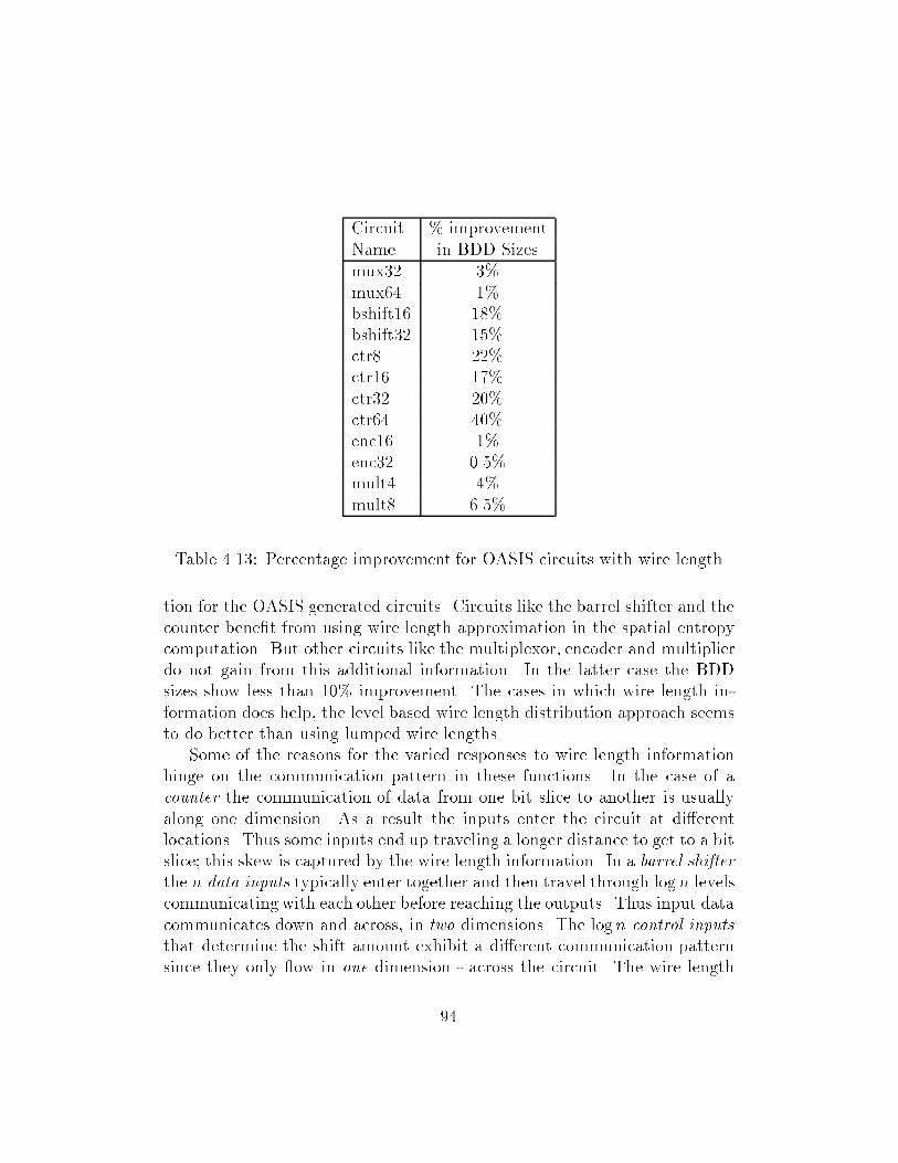
Circuit improvementName in BDD Sizesmux�� � mux�� � bshift�� �� bshift�� �� ctr� �� ctr�� �� ctr�� �� ctr�� �� enc�� � enc�� ��� mult� � mult� ���
Table ����� Percentage improvement for OASIS circuits with wire length
tion for the OASIS generated circuits� Circuits like the barrel shifter and thecounter bene�t from using wire length approximation in the spatial entropycomputation� But other circuits like the multiplexor encoder and multiplierdo not gain from this additional information� In the latter case the BDDsizes show less than �� improvement� The cases in which wire length information does help the level based wire length distribution approach seemsto do better than using lumped wire lengths�Some of the reasons for the varied responses to wire length information
hinge on the communication pattern in these functions� In the case of acounter the communication of data from one bit slice to another is usuallyalong one dimension� As a result the inputs enter the circuit at di�erentlocations� Thus some inputs end up traveling a longer distance to get to a bitslice� this skew is captured by the wire length information� In a barrel shifterthe n data inputs typically enter together and then travel through log n levelscommunicating with each other before reaching the outputs� Thus input datacommunicates down and across in two dimensions� The log n control inputsthat determine the shift amount exhibit a di�erent communication patternsince they only �ow in one dimension across the circuit� The wire length
��

information captures some of this variation in the communication patternbetween the control inputs and the data inputs� Multiplexors and encodersare variations of the selection function� In the multiplexor one of �n inputcombinations gets selected with the help of log n bits of select lines� Inthe encoder one of �n input combinations gets selected and encoded intolog n output lines� These functions require two dimensional communication�Since all the �n input combinations are involved in each output functionthe in�uence of each input variable is equal� They all end up traveling anapproximately equal amount to get to the output causing wire lengths to bea nonfactor� Multipliers are also functions with twoway communication andwith equal participation from each input variable causing wiring skew to beabsent� In addition the family of �integer� multiplier functions have beenproven to have exponential BDD sizes regardless of ordering �Bry���� So thechanges caused by wire lengths can only be minor perturbations�Let us now look at decoders� Table ���� �page ��� shows that decoders
are immune to any kind of wire length approximation� Their BDD sizesare the same regardless of wire length information� The reason for this isfundamental to the nature of the decoding function� In a completely speci�edn input �n output decoder each output of the decoder is speci�ed by exactlyone minterm of the n variable function� For example in a � to � decodero� � a�b�� o� � a�b� o� � ab� and o� � ab� Hence the BDD for every outputfunction oi requires an ordering on the input variables in a single minterm�In such a situation the size of the BDD will be the same regardless of howthe variables in the minterm are ordered since every variable appears once�
Minimization�Now we illustrate the e�ects of redundancy on spatial entropy based BDDordering� As discussed in our assumptions earlier since the e�ects of mini�mization and wire length approximations are not independent we study themtogether� Table ���� �page ��� shows BDD sizes for the Logic Synthesis ��benchmarks using di�erent wire length approximation strategies� There aretwo rows for each circuit� The �rst row represents sizes when the benchmarkcircuits were minimized using the SIS script algebraic �� The second rowrepresents BDD sizes when the benchmark circuits were minimized using theSIS script rugged �� In both cases no reconvergent fanout removal was per
�this script uses algebraic division while generating kernels and common cubes in thefactoring process�
�This is a more aggressive form of minimization using don�t care extraction of various
��

formed� Table ���� �page ��� illustrates the same results for the much largerISCAS �� benchmark circuits� The average BDD size and the standard deviation in BDD sizes for the two sets of benchmarks is illustrated in Table ����and Table �����In order to try and analyze the e�ects of wiring and minimization sep
arately we illustrate some additional plots� These e�ects are studied in thefollowing order�
A� Minimization with and without wire length for the Logic Synthesis ��benchmarks �LgSynth����
B� Minimization with and without wire length for the ISCAS �� benchmarks�
C� Wire length with and without minimization for the Logic Synthesis ��benchmarks�
D� Wirelength with and without minimization for the ISCAS �� benchmarks�
Minimization e�ects are analyzed by comparing the e�ects of the algebraicscript vs the rugged script� Wire length e�ects are analyzed by comparingthe e�ects of no wire length lumped wire length and level�based wire length�Minimization with and without wirelength LgSynth���We begin by studying the e�ect of minimization with and with out
the use of wire length in spatial entropy computation� This is illustrated inFigure ���� �page ��� for the Logic Synthesis �� circuits� �For space reasonsthe X axis uses Circuit Id numbers instead of circuit names�� The two plotsdepict percentage improvement �positive or negative� in BDD sizes whenthe spatial entropy computation was run on circuits minimized with thealgebraic script versus circuits minimized with the rugged script� Wirelength information was not used in one plot while it was used in the secondplot�Let us look at Figure ���� �page ��� �rst� For the smaller Logic Synthesis
benchmarks we observe that overall there seems to be little change in BDDsize �for the better or for the worse� when using circuits minimized with thealgebraic script versus circuits minimized with the rugged script� This is
also seen in Table ���� �page ��� where the average BDD size varies by�� ��
kinds to reduce literal count�
��

Circuit Circuit $ of NodesId Name No W length Lumped W length Level based W length� alu�a ���� ��� ���
alu�r ��� ���� ���� alu�a ���� ����� ����
alu�r ��� ���� ����� counta ��� ��� ����
countr ��� ��� ����� f��ma ��� �� ��
f��mr �� �� ���� z�mla �� �� ��
z�mlr �� �� ��� �xp�a �� ��� ��
�xp�r �� ��� ���� bwa ��� ��� ����
bwr ��� ��� ����� clipa ��� ��� ���
clipr ��� ���� ���� duke�a ��� ���� ���
duke�r ��� ���� ����� misex�a �� �� ���
misex�r �� �� ����� misex�a ���� ��� ���
misex�r ���� ��� ����� sao�a ���� ���� ���
sao�r ���� ��� ����� vg�a ��� ��� ����
vg�r ��� ���� ���
a � algebraic script� r � rugged script
Table ����� E�ect of wire length and the SIS scripts on the Logic SynthesisBenchmarks
��

Mean � Standard Deviation of BDD sizes�$ of Nodes�Statistic No W length Lumped W Length Level based W length
j V ja ��� ��� ����a���j BDD j� ������ ����� ���
j V jr ����� ��� ����r���j BDD j� ��� ����� �����
Table ����� j V j and � of sizes for Logic Synthesis �� circuits �with minimization and w l approximations�a� algebraic script r� rugged script
Circuit $ of NodesName No W length Lumped W length Level based W lengthc���a ����� ����� �����c���r ���� ���� ����c���a ����� ����� �����c���r ����� ����� �����c���a ����� ����� �����c���r ���� ���� �����c����a ����� ����� �����c����r ����� ����� �����c����a ������ ������ ������c����r � ���� ��� ������ ������
Table ����� E�ect of wire length and the SIS scripts on the ISCAS �� Benchmarksa � algebraic script� r � rugged script
��

��
����
���
���
����
�
���
��
��
���
�
� � � � � � �� �� �� ��
FractionChange
inBDDSize
Circuit Ids
Spatial Entropy Computation without Wirelength
Sizerugged�SizealgebraicSizealgebraic
��
����
���
���
����
�
���
��
��
���
�
� � � � � � �� �� �� ��
FractionChange
inBDDSize
Circuit Ids
Spatial Entropy Computation with Wirelength
Sizerugged�SizealgebraicSizealgebraic
Figure ����� E�ect of Minimization Scripts on the Logic Synthesis Benchmarks
��

��
����
��
����
�
���
�
c�� c�� c��� c���� c���
FractionChange
inBDDSize
Circuit Names
Spatial Entropy Computation without Wirelength
Sizerugged�SizealgebraicSizealgebraic
��
����
��
����
�
���
�
c�� c�� c��� c���� c���
FractionChange
inBDDSize
Circuit Names
Spatial Entropy Computation with Wirelength
Sizerugged�SizealgebraicSizealgebraic
Figure ����� E�ect of Minimization Scripts on the ISCAS �� Benchmarks
���
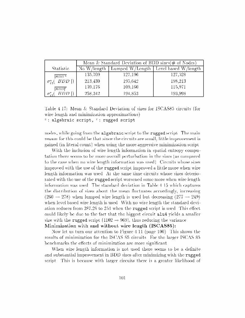
Mean � Standard Deviation of BDD sizes�$ of Nodes�Statistic No W length Lumped W Length Level based W length
jBDDja������ ������ ������
�a���j BDD j� ������ ������ ������
jBDDjr������ ������ ������
�r���j BDD j� ������ ������ ������
Table ����� Mean � Standard Deviation of sizes for ISCAS�� circuits �forwire length and minimization approximations�a � algebraic script� r � rugged script
nodes while going from the algebraic script to the rugged script� The mainreason for this could be that since the circuits are small little improvement isgained �in literal count� when using the more aggressive minimization script�With the inclusion of wire length information in spatial entropy compu
tation there seems to be more overall perturbation in the sizes �as comparedto the case when no wire length information was used�� Circuits whose sizesimproved with the use of the rugged script improved a little more when wirelength information was used� At the same time circuits whose sizes deteriorated with the use of the rugged script worsened some more when wire lengthinformation was used� The standard deviation in Table ���� which capturesthe distribution of sizes about the mean �uctuates accordingly increasing���� � ���� when lumped wire length is used but decreasing ���� � ����when level based wire length is used� With no wire length the standard deviation reduces from ������ to ��� when the rugged script is used� This e�ectcould likely be due to the fact that the biggest circuit alu� yields a smallersize with the rugged script ����� � ���� thus reducing the variance�Minimization with and without wire length ISCAS���Now let us turn our attention to Figure ���� �page ����� This shows the
results of minimization for the ISCAS �� circuits� For the larger ISCAS ��benchmarks the e�ects of minimization are more signi�cant�When wire length information is not used there seems to be a de�nite
and substantial improvement in BDD sizes after minimizing with the ruggedscript� This is because with larger circuits there is a greater likelihood of
���

performance improvement �in literal count� when the rugged script is usedfor minimization instead of the algebraic script� This is not re�ected in theaverage and standard deviation values in Table ���� �page ���� because ofthe dominating e�ect that circuit c���� has on these statistics� Discountingits e�ect from the computation j V ja � j V jr goes from ���� ��� � ���� ���to ��� ��� � ��� ��� indicating a clear improvement�When wire length information is used the bene�ts of running spatial
entropy computation on the rugged script minimized circuits appear mixed�While the lower plot of Figure ���� �page ���� shows sizes improving withwire length information this is not always the case� In Table ���� �page ���we notice that for circuit c��� minimized with the rugged script the sizesimprove when lumped wire length information is used but they deterioratewhen level�based wire lengths are used� Similarly in circuit c���� minimizedwith the rugged script the sizes improve when level�based wire lengths areused but deteriorate when lumped wire length is used� The statistics inTable ���� �page ���� on the other hand show that there is an improvement inaverage BDD size while going from the algebraic script to the rugged scriptregardless of whether lumped wire length is used ����� ��� � ���� ���� orlevel based wire length is used ����� ��� � ���� ����� This implies that on theaverage the BDD sizes improved more than they deteriorated� The standarddeviation does not show much change ����� ��� � ���� ���� ����� ��� ����� ����� because of the dominating e�ect of c�����The mixed size improvement results for minimization with wire length
con�rms our earlier hypothesis that the e�ects of minimization and wirelength are not independent� While the rugged script does a better job ofremoving redundant literals it also alters the wire length distribution in thecircuit with the excessive levels generated during factoring� This could a�ectthe spatial entropy distribution in the circuit for the better or for the worse�Wire length with and without minimization LgSynth���We now try to analyze the e�ect of wire length on BDD sizes for cir
cuits minimized with the algebraic script and circuits minimized with therugged script� Figure ���� �page ���� shows two plots for the Logic Synthesis benchmarks� The �rst plot in the �gure compares BDD sizes for circuitsminimized with the algebraic script when spatial entropy computation isperformed with and without wire length information� The second plot doesthe same comparison for circuits minimized with the rugged script�For the Logic Synthesis benchmarks minimized with the algebraic script
���

���
���
���
��
���
��
��
���
���
����
� � � � � � �� �� �� ��
BDDSizes
Circuit Ids
Minimization using algebraic script
without wirelengthwith wirelength
���
���
���
��
���
��
��
���
���
����
� � � � � � �� �� �� ��
BDDSizes
Circuit Ids
Minimization using rugged script
without wirelengthwith wirelength
Figure ����� E�ect of Wire Length on the Logic Synthesis Benchmarks
���

�����
�����
�����
����
�����
����
����
�����
�����
������
c�� c�� c��� c���� c���
BDDSizes
Circuit Names
Minimization using algebraic script
without wirelengthwith wirelength
�����
�����
�����
����
�����
����
����
�����
�����
������
c�� c�� c��� c���� c���
BDDSizes
Circuit Names
Minimization using rugged script
������
WLumped
WLevel
WLevel
WLumped
without wirelengthwith wirelength
Figure ����� E�ect of Wire Length on the ISCAS �� Benchmarks
���
�Figure ����� wire length information appears to be useful only when theBDD sizes get bigger �see Circuit Ids �� �� �� ���� As Table ���� �page ��� indicates the average BDD size improvement is quite minimal for these circuitswith wire length information ���� � f���� ���g�� The standard deviationvaries accordingly ������� � f������ ���g�� When the same circuits are minimized with the rugged script even this bene�t seems to disappear� Theaverage BDD size values also indicate this ������� f���� ���g��Wire length with and without minimization ISCAS���Figure ���� shows the same set of results for the ISCAS �� circuits� �The
sizes for circuit c���� have been scaled to ���K nodes to help present resultsclearly� This should not a�ect the results here since we are only interestedin comparative numbers��For the ISCAS benchmarks �Figure ����� minimized with the algebraic
script except for one circuit �c���� the wire length information does seemto bene�t but in varying amounts� Table ���� �page ���� con�rms this assizes improve from ���� ��� to f���� ���� ���� ���g�When minimized with the rugged script the results are again mixed�
but due to the improvement in size of the c���� circuit the overall average BDD size shows in improvement in Table ����� As mentioned earlierwhile wire length information does bene�t the lumped and the level�basedapproximations both fare di�erently�
Reconvergent FanoutFinally we discuss the errors due to reconvergent fanout� As discussed
in Chapter � the procedure to remove these inaccuracies in spatial entropycomputation is very expensive and is exponential in the number of fanoutinputs in the supergate� We implemented the procedure to construct supergates and remover errors in spatial entropy and �probability computation�But our results were unfortunately not very conclusive� For circuits withsmall supergates and a small number of fanout inputs where reconvergentfanout removal was tractable we found that there was not a need to applythe procedure since the spatial entropy computation already yielded goodsizes� For the circuits where the BDD sizes were poor it was very expensiveto apply this procedure because the supergate sizes and fanout inputs werelarge in number� We tabulate in Table ���� the supergate sizes and numberof fanout inputs for circuits in the Logic Synthesis �� benchmark set� In thetable we indicate the number of reconvergent nodes and the largest supergatesize for each circuit� We also indicate the largest number of fanout nodes
���

Circuit Total Reconv� Largest Max $ of $ of F outsName Nodes Nodes Sg Size F out Nodes �� ��alu� ��� �� ��� �� ��alu� ���� ��� ��� �� ���count ��� ��� �� �� �frg� ��� �� ��� �� ���xp� ��� �� �� � �bw ��� �� �� � �clip ��� �� ��� � �duke� ��� �� ��� �� ��misex� �� �� �� � �misex� ��� � �� � �rd�� ��� �� ��� � �sao� ��� �� �� �� �vg� ��� �� ��� �� ��
Table ����� Reconvergent Fanout Information for Logic Synthesis �� Benchmarks
found in a supergate� This is an indication of how wide the supergate is andhow expensive it would be to simulate such a supergate� The last columnis another indicator of reconvergent fanout removal expense� It counts thenumber of supergates that have �� or more fanout nodes� A supergate with�� fanout nodes requires ���� simulations to compute the exact �probabilityand spatial entropy at its reconvergent node� Hence this is a measure of howmany such large supergates exist in the circuit�We observe from Table ��� �page ��� that some of the circuits for which
spent had trouble in generating good BDD sizes were vg�� sao�� frg��
count and alu�� From Table ���� �page ���� we also notice that theseare the circuits that have high reconvergent fanout with several supergatesthat have �� or more fanout nodes� So it is likely that the errors due to thereconvergent fanout in these circuits is contributing to the poor orderings�
���

����� Spatial Entropy Vector Combination Strategies
We study three approaches to combining output spatial entropy vectors inmultioutput functions� maximum �max� weighted�multiply �wmult� andweighted�divide �wdiv�� These were discussed in detail in Section ���� Ourresults are presented in Table ���� and Table ���� for the two benchmarkcircuits with and without wire length approximations� Figure ���� and Figure ���� plot the BDD sizes for the di�erent spatial entropy vector combiningstrategies generated with and without wire length approximation� �The sizesfor circuit c���� have again been scaled to ���K nodes��Let us look at the plot for the Logic Synthesis benchmarks �rst �Fig
ure ������ For most of the small circuits there seems little to choose betweenone combining strategy versus the other� For a couple of the bigger circuits�Circuit Id $s ��� there seems to be a slightly clearer choice of the beststrategy though this is true only when wire length information is also provided� The choice of the strategy seems to vary from circuit to circuit� Thisis also illustrated in the following situation� Looking at Table ���� we observethat for the �arithmetic� circuits in the benchmark alu�� alu�� countthe weighted divide strategy wdiv does not appear to yield good sizes� Itmay be recalled that wdiv is the approach where the spatial entropy vectorvalues are combined such that the cumulative spatial entropy at every output node is normalized to the range ��� ��� All the above arithmetic circuitsprobably have adderlike computing elements in them where the individualoutputs have disproportionate contributions to the total circuit spatial entropy� As a result giving equal importance to all the output spatial entropyvectors using the wdiv approach does not seem to be the right thing to do�On the other hand if we look at circuits sao�� duke�� clip and vg� in Table ���� they seem to bene�t by the wdiv approach� One of the reasons forthis could be the following� These are circuits with high reconvergent fanout�Since we ignore reconvergent fanout removal the errors in the computationprocess may make the spatial entropy at some output nodes unrealisticallyhigh� Using the weighted divide approach forces every output to be treatedwith equal importance thus supressing errors that reconvergent fanout mighthave introduced�Now let us look at Figure ���� that shows plots for the ISCAS �� bench
marks� Here we notice that there is more variation between sizes generatedby one strategy versus sizes generated by another� But the choice of a par
���

Circuit �S Combining $ of Nodes �with Wire Length Approx��Id Name Strategy No W len Lumped Level
max ��� ��� ���� alu� wmult ��� ��� ���
wdiv ��� ��� ���max ��� ���� ����
� alu� wmult ���� ���� ���wdiv ���� ���� ����max ��� ��� ���
� count wmult ��� ��� ���wdiv ��� ��� ���max �� �� ��
� f��m wmult �� �� ��wdiv �� �� ��max ��� ��� ���
� clip wmult ��� ��� ���wdiv ��� ��� ���max ��� ��� ����
� duke� wmult ��� ��� ���wdiv ��� ��� ���max ��� ��� ���
� misex� wmult ��� ��� ���wdiv ��� ��� ���max ��� ��� ���
� sao� wmult ��� ��� ���wdiv ��� ��� ���max ��� ��� ���
� vg� wmult ��� ��� ���wdiv ��� ��� ���
Table ����� Comparision of �S combination strategies for Logic Synthesis ��Benchmarks
���

Circuit �S Combining $ of Nodes � with W length approx��Id Name Strategy No W len Lumped Level
max ����� ���� ������ c��� wmult ���� ���� �����
wdiv ���� ���� �����max ����� ����� ������
� c��� wmult ����� ����� �����wdiv ����� ����� �����max ���� ���� �����
� c��� wmult ���� ���� ������wdiv ����� ����� �����max ����� ����� �����
� c���� wmult ����� ����� �����wdiv ����� ����� �����max ������� ������ ������
� c���� wmult ������� ������ ������wdiv ������� ������ �������
Table ����� Comparision of �S combination strategies for ISCAS �� Benchmarks
���

���
���
���
��
���
��
��
���
���
����
� � � � � �
BDDSizes
Circuit Ids
Spatial Entropy Computation without Wirelength
MaxWmultWdiv
���
���
���
��
���
��
��
���
���
����
� � � � � �
BDDSizes
Circuit Ids
Spatial Entropy Computation with Wirelength
MaxWmultWdiv
Figure ����� �S Combining Strategies for Logic Synthesis Benchmarks
���

�����
�����
�����
����
�����
����
����
�����
�����
������
c�� c�� c��� c���� c���
BDDSizes
Circuit Names
Spatial Entropy Computation without Wirelength
MaxWmultWdiv
�����
�����
�����
����
�����
����
����
�����
�����
������
c�� c�� c��� c���� c���
BDDSizes
Circuit Names
Spatial Entropy Computation with Wirelength
MaxWmultWdiv
Figure ����� �S Combining Strategies for ISCAS �� Benchmarks
���

ticular strategy is unclear� The max and wmult approaches seem to performequally well� We also observe that circuit c��� an ALU�control circuit doesbadly with the weighted divide approach� This appears to con�rm our earlierobservations about using this approach on circuits with uneven contributionsfrom the di�erent outputs�
��� Conclusions
We are now ready to draw some conclusions� For the smaller circuits the spatial entropy approach generates BDD sizes competitive with the optimizationintensive approaches and the static attribute based approaches� But as thecircuits become larger the e�ectiveness of the optimzation intensive strategiesbecomes markedly apparent while both the static attribute based approachand the spatial entropy based approach do poorly but for di�erent reasons�The e�ectiveness of the optimization approach comes from the fact that theywork directly with the BDDs� In contrast the other approaches make approximations while working with an implementation� The static attributebased approaches use level and depth based heuristics while the spatial entropy based approach makes approximations to simplify the computation ofthe attribute� The e�ect of this is apparent as the circuits get larger� Withlarger circuits there is a greater chance that static attribute based heuristicsmay make wrong decisions� Similarly the e�ect of spatial entropy approximations such as reconvergent fanout wire length and redundancy is moresigni�cant in larger circuits� This results in poor orderings� The e�ect of apoor ordering on the BDD sizes is more signi�cant in large circuits� This isbecause a BDD size can grow exponentially at successive levels in the graphand a wrong variable choice at one level �in a large circuit� could explodeinto a huge BDD within a few levels� The optimization intensive approachesdirectly search the space of orderings while building the BDDs thus avoidingthe need to examine an implementation�But optimization intensive approaches pay a big price in the time they
spend searching for a good ordering� Most static attribute based approachesrequire a simple �breadth �rst or depth �rst� traversal through the networkthat consumes a few minutes� For instance the spatial entropy approachtook ����� seconds on a DEC Station ���� to generate an ordering for theISCAS circuit c���� In contrast the minwid�� approach was documented
���

�ISY��� as taking approximately ����� seconds on a SPARC Station ���How do inaccuracies in computing the spatial entropy attribute a�ect
variable orderings and BDD sizes� We �nd that for regular structured circuits where the communication pattern is wellde�ned the e�ects of wirelength can be observed clearly� These e�ects are a function of the communication behavior in these circuits� Consequently some circuits bene�t fromthis information generating smaller BDDs while others do not� For the moreirregular circuits �as in the benchmark sets� the e�ect of wire length is mixed�For the smaller benchmark circuits computing spatial entropy without wirelength information does not hurt BDD sizes� For the larger circuits wirelength information helps improve sizes but not always� The degree of minimization in the circuit and the communication pattern in the circuit controlthis e�ect�Lack of minimization a�ects spatial entropy computation and BDD sizes
signi�cantly in the larger circuits� Hence in such circuits minimization isbene�cial and improves BDD sizes� But when wire length information isalso used in these minimized circuits the approximations made in distributing wire lengths in�uence the e�ects of minimization� We had stated inan earlier section that the factors of logic minimization and wire length areinterdependent and these results con�rm it�Reconvergent fanout seems to have a de�nite in�uence on spatial entropy
computation for larger circuits as we found a correlation between poor oderings and heavy reconvergent fanout in some of these circuits� But the extentof its e�ect cannot be clearly estimated� This is because it was computationally too expensive to remove the errors in spatial entropy computation�due to reconvergent fanout� in these large circuits� Since minimization canchange the structure and organization of the gates in the circuit it is likelythat the minimization process can introduce or remove reconvergent nodesin the circuit� This also makes it di�cult to attribute the cause of poororderings in these circuits entirely to reconvergent fanout errors�With respect to the spatial entropy vector combining strategies the max
and wmult approaches do not perform very di�erently from each other� Thiscould be because both approaches combine output spatial entropy vectors inproportion to the output spatial entropy values� The wdiv approach forcesevery output node to contribute equally� Since this may not always be thecase this approach does not do well in some circuits� On the other hand itdoes help yield good orderings in cases where excess spatial entropy contri
���

bution gets generated due to reconvergent fanout or wire length distributionapproximations�On the whole the spatial entropy computation approach does use approx
imations that a�ect the accuracy of the attribute� But the e�ects of theseapproximations are felt more signi�cantly in the variable ordering problemespecially on large circuits than they might be in other applications of thisattribute� The �rst reason is the �ne granularity with which the attribute isbeing handled� Orderings are generated on spatial entropy vectors and notspatial entropies themselves� Thus inaccuracies get further distributed fromthe spatial entropies on the nodes to the spatial entropy contributions in thevectors� The second reason is the extreme sensitivity of BDDs to variableorderings� A small error in spatial entropy computation that yields a di�erent ordering can translate into a BDD that is several thousand nodes largerin size when the circuit is large�Due to the approximations in spatial entropy computation the exper
imental evidence for spatial entropy based variable ordering has not beenconclusive� We simultaneously explored a theoretical basis for using the spatial entropy of an implementation to generate BDD variable orders� The sizeof a BDD is a characteristic of the function and is invariant over di�erentimplementations� Then how can the spatial entropy of an implementationof the function be capable of generating variable orders for the BDD� Thiscan only be possible if the spatial entropy of an implementation capturesa fundamental characteristic of the function� This is the focus of the nextchapter�
���

Chapter �
Spatial Entropy as a Measure of
Area�Complexity
This chapter draws on some of the conclusions in Chapter �� In order to explain a theoretical basis for using spatial entropy to generate BDD variableorders an important question that needed to be answered was� If a BDD isa characteristic of the function then how can the spatial entropy of someimplementation of the function generate variable orders� In this chapter weshow empirical evidence that the spatial entropy of an implementation is capable of measuring the gatecount complexity of the function� This providesempirical evidence that spatial entropy is capable of capturing function behavior� We also show that our de�nition of gatecount complexity in booleanspace called information content does a good job in estimating actual logicgate cost and there is strong correlation between information content andgate count�We begin with some motivation for the work in this chapter and then
provide background information on boolean functions and complexity� InSection ��� we de�ne our estimate of gatecount complexity in boolean space�In order to show that spatial entropy can be used to measure gatecount complexity we introduce a notation called the decision tree in Section ���� Thisis an intermediate representation relating a function and its implementation�We then illustrate in Section ��� how the spatial entropy of an implementation can be computed using the decision tree and how this computation isapproximated by the gatelevel spatial entropy procedure discussed in Chapter �� Section ��� discusses experimental results to correlate spatial entropy

and information content and gatecount complexity and information content�
��� Motivation
In the previous chapter we demonstrated empirically that the spatial entropybased approach can generate variable orders for binary decision diagrams�We also observed that factors that a�ect the accuracy of spatial entropycomputation �in a given implementation� like reconvergent fanout and poorestimates of wire length have a signi�cant e�ect on BDD sizes� Spatialentropy is also in�uenced by logic minimization� Di�erent implementationsof the same function can di�er signi�cantly in their spatial entropy valuesdue to di�erent degrees of minimization in each implementation�Along with the experimental work we explored a theoretical basis to
connect spatial entropy and BDD variable ordering� The size of a BDDis a characteristic of the function� it is invariant over di�erent implementations� Then how can the spatial entropy of an implementation generatevariable orders for the BDD� In order to do so the spatial entropy of theimplementation must be able to capture some characteristic of the function!sminterms� But our experiments in Chapter � showed that there can be widevariations in the spatial entropies of the same function when computed ondi�erent implementations� So this raised the question� what should be thebest implementation to capture this function behavior and why�Spatial entropy is the dynamic communication e�ort required to compute
the function� In a physical �CMOS� implementation this becomes the switching energy expended by the circuit while computing the function� Over allimplementations of a given function the one with minimum spatial entropyhas minimum switching energy and describes the minimum communicatione�ort needed to compute the function� Thus the minimum spatial entropyover all implementations of a function acts like a signature of the functionsince it provides a lower bound on the switching energy over all implementations of that function� Minimum spatial entropy in an implementationimplies simultaneously minimizing the logic gates and the wires in the implementation� This yields minimum switching energy because the switchingactivity at the gates �that contribute to the power consumption� is minimized due to lesser gates and the delay at each gate is minimized due toreduced switching capacitance and shorter wires� So comparing a pair of
���

implementations with minimum spatial entropy is equivalent to comparingthe behavior of the underlying functions �in the two implementations��But as we noticed in Chapter � generating minimum spatial entropy im
plementations is di�cult with existing logic minimization tools� These toolsonly perform logic minimization and ignore the e�ect of wires� As Figure ���showed minimizing gate count can generate longer wires yielding greaterspatial entropy �and switching energy�� In such a situation an approximation can be made� A minimal gate count implementation on which spatialentropy is computed with unit wire length can be used as an approximationto a minimum spatial entropy implementation computed with actual wirelengths� This minimal gate count implementation also acts like a signatureof the function� This is because even this approximate spatial entropy �computed with unit wire length� provides a lower bound on a physical attributethe gate count over all implementations of that function�How does the spatial entropy of a minimal gate count implementation
capture minterm characteristics and boolean function behavior� We answerthis question in this chapter by studying minimality and spatial entropyin boolean space in the context of boolean function complexity� The com�plexity of a boolean function is a measure that provides a lower bound onsome physical attribute over all implementations of that function� Thus itis a fundamental characteristic of function behavior� Depending upon thephysical attribute that it bounds the complexity can be de�ned di�erently wiringcomplexity layoutarea complexity activearea complexity energycomplexity etc�� We are interested in the gate�count complexity the cost ofgates in an implementation� In this chapter we de�ne information content anestimate of the gatecount complexity of boolean functions over its mintermsand illustrate empirically that spatial entropy is a linear function of information content� While this does not give us a theoretical basis for using spatialentropy for BDD variable ordering it yields empirical evidence that sucha basis can exist by demonstrating that spatial entropy can track functionbehavior� We also show that information content and spatial entropy can actas measures of actual gatecount complexity�We begin with some background on boolean functions and then discuss
related work in function complexity�
���

��� Background
����� De�nitions
We start by de�ning some frequently used terms� A boolean variable is avariable that takes a value from the set f�� �g� A literal is a �boolean� variableor its negation� For example a and a� are literals� A single�output booleanfunction of n input variables f�x�� � � � � xn� is of the form�
f � f�� �gn �� f�� �g
When the function f is of the form
f � f�� �gn �� f�� �gm
then we have a multioutput boolean function �ninput moutput�� We shallrestrict ourselves to single output functions for the present�A product term is a conjunction �logical AND� of input literals� For
example ab�c is a product term with implicit conjunction� A minterm is aproduct term where every input variable is represented in its complementedor uncomplemented form� The ON�set of a function is the set of mintermsfor which the function has a value of �� The OFF�set of a function is the setof minterms for which the function has a value of �� The DON�T CARE�setof a function is the set of minterms for which the function can have a valueof � or �� A completely speci�ed function f is one in which each minterm isassigned a unique value either a � or �� In an incompletely speci�ed functionthere are minterms that may be a � or � i�e� the DON!T CAREset is notempty�A sum�of�products expression is a boolean function representation ex
pressed as a disjunction of product terms� Here is an example�
f � ac� ad�e� bc� bde
This is also called a two�level expression because it has two levels of logic�ANDOR�� A function can also be represented as a multi�level expressionwith more than two levels of logic� For example the above function f wouldappear as
f � �a� b��c� de�
���

A minimal expression is a multilevel expression with the fewest number ofliterals�An alternative way to view an nvariable boolean function is as an n
dimensional hypercube �f�� �gn�� Figure ��� shows a boolean function of �variables a� b� c represented as a �dimensional hypercube� The vertices of thehypercube denote the minterms� For example the vertex ����� represents theminterm a�bc�� A cube is a collection of minterms of an nvariable functionwhere the number of minterms is a power of � �m for some m � n� Ifm � � then the cube has only � minterm which is a vertex of the hypercube� If � � m � n then for each of the �m minterms the literals have thesame value in n � m positions and one of �m combinations in the other mpositions� Algebraically a cube is a product term� for example the cube withthe minterms f���� ���g is the product term b�c�� Viewed on a hypercube acube is a projection of the hypercube along one or more dimensions whereeach dimension corresponds to an input literal� This yields an m dimensionalrectangular subspace of the hypercube f�� �gn� For example projecting the�dimensional hypercube along the dimension of literal b yields a cube ofdimension � with �� � � minterms f���� ���� ���� ���g whose algebraic product term equivalent is b� A cube c is a subset of another cube c� if all theminterms in c are contained in the minterm set of c�� For example the cubef���� ���g is a subset of the above cube�The Shannon expansion of a boolean function f on the variable xi is
f�x�� x�� � � � � xn� � x�i�f�x�� � � � � xi � �� � � � � xn� � xi�f�x�� � � � � xi � �� � � � � xn�
where f�x�� � � � � xi � �� � � � � xn� and f�x�� � � � � xi � �� � � � � xn� are partial func�tions that represent the values of f when the input variable xi has value of� and � respectively� These partial functions are called boolean cofactors orShannon cofactors of the function with respect to x�
We now brie�y summarize related work in function complexity� Thecomplexity of boolean functions has been de�ned over the years with boundson di�erent physical attributes depending on the implementation technology�It was �rst investigated by Shannon �Sha��� while studying twoterminalswitching networks with relay contacts� Muller �Mul��� then applied hisresult to networks with logical elements and showed that an upper bound onthe complexity of single output networks was of the order of �n
nwhere n is
the number of input variables� Then Kellerman �Kel��� derived an empirical
���

(000)(100)
a
b
c
(110)
(111)
(101)(001)
(011)
(010)
Figure ���� A Cube Space Representation of a � Variable Function
formula to estimate the average cost of a combinational logic network as afunction of the number of ONterms in the cube space of the function� Heillustrated his results for singleoutput networks using diodes and modulesas the implementation technology� This was followed by work on entropybased de�nitions of complexity by several researchers �Hel�� CF�� Mas��Pip�� CA��� with bounds on attributes like diode counts gate counts andliteral counts� These were discussed in detail in Chapter �� Yao �Yao���used a communication model to to formulate lower bounds on the worst caseinformation complexity of a boolean function f and this was also discussedin Chapter ��How does our work relate to the above research� In the next section we
de�ne the gatecount complexity of a boolean function by its informationcontent� This de�nition di�ers from the existing de�nitions in that it emphasizes on the spatial distribution of the �s and �s in the cube space ratherthan just the number of �s and �s in the cube space� One of the motivationsfor doing so is to be able to predict the cost of implementing the function notjust in terms of the literal count or gates but also in terms of the communication between the gates through wiring� Our de�nition is entropy based andis de�ned for completely speci�ed singleoutput functions� The de�nitionensures minimality for twolevel function representations and is an estimateof gatecount complexity in a multilevel implementation�
���

��� Information Content
We begin this section with an intuitive development of our idea� Our objective is to de�ne the gatecount complexity of a boolean function in terms ofthe spatial distribution of minterms ��s and �s� in the cube space� This willgive us an estimate of the cost of implementing the function�Let us start by trying to understand the spatial embedding of minterms
and see how it contributes to the complexity of the function� Consider a setof completely speci�ed singleoutput �variable functions� Figure ��� illustrates an example collection of such functions and their minterm distributionin cube space� The ONterms or �s are marked with a � at the cube vertex�The unmarked vertices represent the OFFterms or �s� The minimized expressions for these functions are also shown� Let us assume for the sake ofthese examples that the cost of the implementation is measured by the literalcount in the minimized twolevel expression� Consider functions A and F �Both are �variable functions that have exactly four �s in their cube space�But the cost of implementingA is more than the cost of implementing F using the literal count measure� The reason for this is the spatial arrangementof the �s in the cube space� This was also observed in �Kel��� and �CF����Their experimental data showed that the maximumcost data point �for afunction of n variables with u �s in the cube space� appeared when none ofthe �s could be covered while the minimumcost data point appeared whenall the �s were optimally covered�On a �ner grain consider functions C and D� Both have exactly two �s in
their cube space� But the spatial arrangement of the �s permitsD to achieve acheaper implementation though this would require a �ner cost discriminatorthan the simplistic measure of twolevel literal count� Functions B and Eexhibit a di�erent feature� Here the number of �s outnumber the number of�s� The function E contains six �s and two �s and the two OFFterms arein almost identical spatial positions as the two ONterms of function C� Sowith respect to spatial distribution the two functions �E and C� look verysimilar� Their implementations too have the same cost�Now that we have an intuitive idea of why spatial embedding of minterms
can a�ect gatecount complexity of functions we can formally de�ne ourmeasure for completely speci�ed singleoutput functions� We begin with afew de�nitions�
���

A = a’b’c’ + a’bc+ab’c + abc’
B = b + ac’
F = ac + a’c’
E = a’b’ + bc + ac’
D = a(bc + b’c’)C = ab’c’ + a’bc
c
b
a
Figure ���� Example functions of � variables a� b� c
���

De�nition � A monochromatic cube c of a function f is a cube suchthat m � c �f�m� � �� � �f�m� � ��� where m is a minterm of thefunction f that belongs to cube c� and f�m� is the value of the function f forthe minterm m� When f�m� � � then the cube is termed a one�cube� c��When f�m� � � the cube is termed a zero�cube� c��
De�nition � The size of a cube j c j is the number of minterms in the cube�
De�nition � A k�decomposition Dk of a boolean function is a union�O � Z� of a set of one�cubes O� and a set of zero�cubes Z such that k �j O j� j Z j and O � Z is a partition of the function�s cube space�
De�nition � A minimum k�decomposition of a boolean function is a k�decompositionDk with the smallest k such that for any other k��decompositionDk� of the same boolean function� either k k�� or if k � k�� then the sumof the cube sizes in k is greater than the sum of the cube sizes in k��
Xci�fOk�Zkg
j ci j �X
c�i�fOk��Zk�g
j c�ij
Since cubes can overlap the sum of the cube sizes in a minimum kdecomposition does not have to be bounded by the number of minterms �n�The monochromatic cubes de�ned here are an ndimensional equivalent of
the monochromatic rectangles used by Yao in his communication complexitymodel �Yao���� A monochromatic cube is a collection of minterms �in the ndimensions� for which the function value is constant �� or ��� The monochromatic rectangle de�ned by Yao also describes a collection of minterms witha constant function value� But the rectangle is de�ned di�erently� The inputn bits are partitioned into bn��c and dn��e halves� The set M consists ofthe �bn��c values in one half while N consists of the �dn��e values in the otherhalf� The rectangle is a cross product P � Q � M �N where P � M andQ � N �Before we move further let us review the examples in Figure ��� �on
page ����� The minimum k�decomposition of the functions into monochromatic one zerocubes is shown in Figure ��� �on page ����� In function Aall the onecubes and zerocubes are of size �� The rearrangement of theONterms in the cube space of function F results in larger cubes �of size ���Functions C and D di�er in that the arrangement of minterms in D!s cube
���

space yields a zerocube of size � while the minterm distribution in C onlypermits zerocubes of size �� This contributes to the sharing in the implementation of D� The other observation of note is that the monochromaticdecomposition of cubes for C and E are similar except for the onecube andzerocube distribution being reversed�In the following subsection we show how the minimum kdecomposition
of cubes relates to results in twolevel logic minimization�
����� k�decomposition and Two�level Minimization
Twolevel logic minimization addresses the problem of minimizing the number of literals in a twolevel representation of a boolean function� The objective is to generate a minimal form of the function that is prime and ir�redundant� A function is irredundant if and only if no product term can bedeleted without changing the function� Conversely redundant terms can beremoved without changing the function� A product term is prime if and onlyif all literals in the term are necessary� Any nonprime term can be expandedby removing one or more literals without a�ecting the logic function� Thusthere are two basic strategies� expansion and redundancy removal�In the early years of logic design twolevel logic minimization was
performed with the use of Karnaughmaps �Koh���� The monochromaticone zerocubes in our de�nition bear a resemblance to them� SubsequentlyQuine and McCluskey �McC��� introduced more sophisticated techniques fortwolevel minimization like prime implicant generation and minimumprimecover extraction that have formed the basis for almost all of twolevel logicminimization today�Regardless of the technique the objective in twolevel minimization is to
generate a minimal form of the function that is prime and irredundant� Wenow show that a minimum kdecomposition of a function into monochromatic one zerocubes guarantees a prime irredundant minimized form of thefunction�
Lemma � A minimum k�decomposition guarantees an irredundant cover ofthe function�
Proof by contradiction� Suppose there exists a minimum k�decompositionthat has a redundant product term in it� A product term corresponds to a one�cube� and since it is redundant� we can remove it� This implies removing the
���

A F
B E
C D= ab’c’ + a’bc = a(bc + b’c’)
= a’b’c’ + a’bc + ab’c + abc’ = ac + a’c’
= a’b’ + bc + ac’= b + ac’
Zero Cube
One Cube
Figure ���� Monochromatic Cube Decomposition for �Variable Functions
���

cube from the decomposition set� giving us a decomposition of the functionthat is smaller than what we started with� This contradicts our assumptionthat we had a minimum k�decomposition initially��
Lemma � A minimum k�decomposition guarantees that all the literals inthe two�level minimized form of the function are necessary�
Proof by contradiction� If a literal were not necessary in a minimum k�decomposition� then it means that it can be expanded out from its minterm�This would mean that we have just doubled the size of the one�cube containingthat minterm� If the sum of the cube sizes before expansion was �� and ifliteral expansion does not introduce a redundant cube then the sum of thecube sizes after expansion will be at least �� �� This is because the smallestcube is of size and it will produce an increase in size of when doubled�But if the cube size did increase then this implies that we did not start witha minimum k�decomposition see De�nition ���
Lemma � A minimum k�decomposition of a boolean function guarantees aminimized two�level representation that is prime and irredundant�
Proof� From the Lemma on irredundancy� and Lemma � on primality��
Generating a minimum kdecomposition of monochromatic cubes for agiven function is an NPcomplete problem �GJ��� just as problems in traditional twolevel logic minimization are NPcomplete� generating all primeimplicants is O��
n
n� �BHMSV��� while extraction of a minimum prime cover
is NPcomplete �GJ����For a given function the minimum kdecomposition need not be a unique
decomposition� For example Figure ��� shows a decomposition of a functioninto monochromatic one zerocubes in two distinct ways�Before we de�ne a formal expression to estimate gatecount complexity
in terms of these monochromatic cubes we describe certain characteristicsof these cubes and intuitively motivate their role in de�ning this complexity�We will also use the examples in Figure ��� to illustrate the importance ofsome of these characteristics�To start with we need to strengthen the simplistic twolevel literal count
measure that we assumed as the gate cost of an implementation� Ideally the
���

a
b
c
E = a’c + b’c’ + ab E = a’b’ + bc + ac’
Figure ���� Two di�erent Minimum Decompositions for a Function
implementation cost should include the gatecount and the total wiring areabetween the gates� We examine cube characteristics by studying both thesecosts but our formal de�nition is only in terms of gatecount complexity� Inthe following discussion we intuitively explain how cube characteristics cancontribute to gatecount complexity and wiring complexity�
Distribution of One�Zero�cubes� Consider the distribution of the oneand zero cubes in the minimum kdecomposition of a function� Sincethe onecubes determine the onterms in the function and the zerocubesdetermine the o�terms the distribution of onecubes versus zerocubeshas a direct e�ect on the sizes of the ON and OFF sets of the function�This in turn can in�uence implementation cost� Suppose the numberof onecubes is much larger than the number of zerocubes� This skewin the distribution will mean that there is a good chance that the onterms can be minimized to yield a cheap implementation� At the sametime there is also a good chance that because there are few zerocubesimplementing the OFF set of the function and inverting its outputwill also yield a cheap implementation� A more uniform distribution ofone zerocube will make both these tasks more di�cult� Thus a skewed
���

cube distribution reduces the complexity of the function�
Sizes of One�Zero�cubes� The second factor is the sizes of the cubes inthe minimum kdecomposition of a function� The sizes of the cubesdetermine the number of literals in a minimized form of the function�The number of literals in the minimized form in turn in�uences thegate count and thus the cost of the implementation� For instance inthe earlier examples we notice that the literal count in B is less thanthat in A� While A has cubes that are very small in size B has largercubes� in fact one cube is of size � contributing only one literal to theminimized form�
Number of One�Zero�cubes� The third cube characteristic is the numberof cubes in the minimum kdecomposition of a function� This is di�erent from the issue of onecube versus zerocube distribution� We areconcerned here about the total number of onecubes and zerocubes�Take functions A and F in the above example� Both have an equalratio of onecubes��zerocubes � �� �� � �� �� But A has � onecubeswhile F has only � onecubes� This is a consequence of the spatialdistribution of minterms in cube space� The number of onecubes is are�ection of the degree of sharing that is permissible between parts oflogic in an implementation� The greater the number of onecubes themore spatially distributed are the minterms of the function� As a resultthere is less sharing possible not only between cubes but also betweenthe literals in the cubes� For instance in function A the cubes ab�c� andabc can share the literal a in the implementation a�bc� b�c��� but thegain is not as much as compared to F where the single onecube �consisting of ab�c� and abc�� yields ac� in the implementation� The lessersharing permitted also implies more cost in combining the cubes andliterals to implement the function� This means more gates or wires inthe implementation to perform the combining�
Variance of One�Zero�cube Sizes� Finally we consider the e�ect of thesize distribution of cubes in a minimum kdecomposition of the function� A function in which there is a greater variance in the sizes of theonecubes �or zerocubes� will tend to exhibit greater wiring complexity in the implementation� This complexity arises due to the spatialdistances between gate implementations of di�erently sized cubes� The
���

function B above has onecubes of sizes � and � but it is too small anexample to capture the e�ect� Consider a �� variable function with awide variance in the onecube sizes ��� �� �� ���� ���� � � �� of its minimumkdecomposition� In order to implement a cube of size � �c�� one wouldrequire � of the �� literals to be present in the implementation� Onthe other hand a cube of size ��� �c��� would only require � literals inits implementation� Regardless of how the � literals in c� are factoredand implemented there is likely to be some disparity in the size of thelogic required to implement c� versus c��� Sharing amongst cubes andliterals may reduce some of this disparity� But for the implementationas a whole there is likely to be a need for more wiring when di�erentlysized cubes are combined� This wiring e�ect will not be as evident ina function with a lesser variance on cube sizes� Whether the cube sizesare small or big the cones of logic implementing them will approximately be of the same size� Again sharing and factoring can changethis to an extent�
While we have discussed each cube characteristic individually it needs tobe emphasized that the actual implementation cost is the result of a complicated interaction of all these factors along with variations introduced bymultilevel logic minimization and technology mapping� We have tried to explain intuitively how cube characteristics can in�uence implementation costin terms of gatecount and wiring� We now de�ne a formal estimate for gatecount complexity called information content that captures the e�ects of factors � � and � above in the implementation cost� Since the de�nition doesnot capture the e�ect of factor � �variance in cube sizes� which contributessigni�cantly to wiringcomplexity we only de�ne gatecount complexity here�
De�nition � Given a minimum k�decomposition Dk of a boolean functionf into a set of one�cubes O� and a set of zero�cubes Z� where j O j � j Z j� k�the information content I�f�Dk� of the function is de�ned by�
I�f�Dk� �h
jOjjOj�jZj � log�
�jOj�jZjjOj
�� jZj
jOj�jZj � log��jOj�jZjjZj
�i�hP
c��Ojc�j�n� log�
��n
jc�j
��P
c��Zjc�j�n� log�
��n
jc�j
�i
where c� is a one�cube and c� is a zero�cube�
���

We have de�ned information content as the product of two entropy functions� The sizes of one�zero�cubes are captured by the �log� sub terms in the
entropy expression jc�j�nlog��
�n
jc� j� and jc�j
�nlog��
�n
jc�j�� The number of one�zero�
cubes is captured by accumulating these sizes overP
c��O andP
c��Z� Thedistribution of one�zero�cubes is captured by the two binary entropy functions in the de�nition�Why were the two entropy functions multiplied� In information theory
the entropy of two systems is usually expressed as the sum of their individualentropies� For instance suppose we wished to combine the entropies of a pairof bit strings nbits long and mbits long respectively� If we denote an eventby a combination of bits in a bit string then there are �n possible events inthe nbit string and �m possible events in the mbit string� Since entropy isexpressed as the logarithm of the number of possible events the individualentropy in the former case is n and in the latter case is m� Since the events inthe nbit string are independent of those in the mbit string taken togetherthere are �n�m events in all and the entropy of the combined string pair islog��n�m� � n � m� In our de�nition the �rst entropy function describesthe distribution of one zerocubes only in terms of the number of cubeswhile the second entropy function describes their distribution in terms ofthe minterms in the cubes� These are not independent of each other� Thedistribution of the minterms amongst the cubes also in�uences the numberof cubes irrespective of whether they are onecubes or zerocubes� Since thetwo entropy functions have a combined e�ect on the gatecount complexityof the function we take their product�The entropy based de�nition of information content in cube space is an
indicator of minimality in twolevel function descriptions� This is becauseit is de�ned over a minimum kdecomposition of the cubes� and we provedthat this is equivalent to the minimized �prime irredundant� twolevel representation of the function� In fact the literal count in a twolevel functiondescription is part of the de�nition of information content in De�nition ��The term log��
�n
jc�j� represents the number of literals in the minimized cube
c�� Suppose n � � and the cube had � minterms i�e� j c� j� � then thenumber of literals in the minimized cube would be �� For example if a� b� cwere the three variables in the function and the minterms were abc and abc�then the minimized cube is ab which has � literals� This can be determinedfrom log��
��
���
���

As mentioned earlier the objective of this de�nition was to capture thee�ects of the various cube characteristics that in�uence gatecount complexity in multilevel implementations� We experimented with various other estimates before settling upon this de�nition as an estimate of gatecountcomplexity� Some of these estimates are shown below�
�� Literal count in a minimized twolevel expression�
log���n
j c� j� � log���n
j c� j�
�� Entropy function of one zero cube sizes�
Xc��O
j c� j�n
� log���n
j c� j
��Xc��Z
j c� j�n
� log���n
j c� j
�
�� Entropy function of number of one zero cubes�
j O jj O j � j Z j � log�
�j O j � j Z jj O j
��
j Z jj O j � j Z j � log�
� j O j � j Z jj Z j
�
�� Weighted entropy function of cube sizes�
I�f�Dk� �hlog�
�jOj�jZjjOj
��Pc��O
jc� j�n� log�
��n
jc�j
�i�h
log��jOj�jZjjZj
��Pc��Z
jc�j�n� log�
��n
jc�j
�i
In order to study minimality in multilevel functions and de�ne spatialentropy in cube space we introduce a notation called the decision tree inthe next section� It is an intermediate representation that we use to bringtogether a function and its implementation� The information content is acharacteristic of the function and its minterm distribution� In Section ��� weuse the decision tree to establish a relation between the spatial entropy of agiven implementation and the information content of its underlying functionand show how spatial entropy can capture function behavior�
���

��� Decision Tree
Given a kdecomposition for a function how does one construct an implementation for such a function� Before we answer this question let us tryand visualize what the implementation must do� An implementation acceptsas input a minterm m whose literals are spatially distributed� Its task isto decide if the given minterm m is an onterm or if m is an o�term� Ifa naive approach is adopted this would require all the onterms or all theo�terms to be examined� But since several onterms and o�terms share literals and cubes the implementation!s task can be simpli�ed� It would besu�cient if the implementation is able to decide that m � c� or m � c�
where c� is a onecube and c� is a zerocube� One can intuitively see thatsuch a decision would be easier to make when the function has a large number of onterms �j ONset j��j OFFSet j� or a large number of o�terms�j ONset jj OFFSet j�� The di�culty in making such a decision iscaptured by the complexity of the function� In Section ��� we de�nedthe gatecount complexity as the information content de�ned over the kdecomposition of the one zerocubes� As we shall see later spatial entropyis de�ned as the e�ort required to make such a decision thus capturing themeasure of di�culty or the measure of information content�Suppose we are given a kdecomposition of the one zerocubes of a func
tion� We are now interested in understanding how an implementation usesthis kdecomposition to make decisions of the above nature with respect toan input mintermm� We introduce a representation called decision tree thatillustrates this decision process� The decision tree also gives us an insight intoconstructing an implementation for the function from its kdecomposition�We �rst illustrate the decision process for a simple example following
which we formally de�ne it� Consider a � variable function f � ab � cd�Figure ��� shows the kdecomposition for this function where k � �� Thearrows indicate the one and zerocubes �k � �� which are numbered below�
�� a�d� zerocube�
�� b�d� zerocube�
�� b�c� zerocube�
�� a�c�d zerocube�
���

a
b
c
f = ab + cd
d=0 d=1
#2−b’d’
#5 − ab
#6 − cd
#1 − a’d’
#3 − b’c’
a
c
b
#4 − a’c’d
Figure ���� Minimum �decomposition of f � ab� cd
�� ab onecube�
�� cd onecube�
Using the cube numbers to identify them we have a onecube set O �f�� �g and a zerocube set Z � f�� �� �� �g�The decision that we would like to make is� given an input minterm m
with an assignment of boolean values to the literals a� b� c and d which of these� cubes does it belong to� More speci�cally we are interested in determininga subset M of monochromatic cubes where M � O or M � Z such that theinput minterm m � M � At the outset the input decision space of one zerocubes is represented by the �decomposition D� � f�� �� �� �� ��� ��g wherethe onecubes are marked with a �� With successive assignments to theinput literals a� b� c and d we can start making decisions to generate smallersets of current candidate cubes� Suppose we started with the literal a� Theassignment a � � tells us that the variable a is a � in the input m� From
���
Figure ��� this tells us that the inputmmust lie in one of the cubes �� �� ��� ���Similarly if a � � then m must lie in cubes �� �� �� �� ��� Thus the candidatecube sets now are f�� �� ��� ��g and f�� �� �� �� ��g� Since neither of them isa monochromatic cube set we continue making assignments� This process isillustrated in Figure ���� We now consider assignments to the literal b� Fora � �� b � � we discover that the input must lie in cubes ��� ��� Since we nowhave a monochromatic cube set the decision process terminates along thispath� This tells us that if the input m is assigned a � �� b � � then it is partof some minterm in the onecubes �� or �� in the ONset� The assignmentsa � �� b � �� a � �� b � � and a � �� b � � all yield subsets of D� noneof which are monochromatic� Hence the literal assignment continues alongthese paths� The decision process completes when every path terminates in amonochromatic cube setM whereM � fO�Zg� As Figure ��� indicates thisyields a tree that has captured the decision process� This is called the decisiontree� For a given kdecomposition Dk the decision tree is not always unique�A di�erent sequence of literal assignments can yield a di�erent decision tree�Figure ��� illustrates the decision tree for the assignment sequence a� c� b� dfor the same �decomposition of f � ab� cd� This is di�erent from the onein Figure ��� which used the assignment sequence a� b� c� d�We are now ready to state some de�nitions� We �rst de�ne an ordering �
on the input variable set I� The ordering function � generates a permutationon the indices of the input variable set I by assigning an index to eachvariable in I� Given a set of one zerocubes representing the kdecompositionDk for a function and an ordering � on the input variable set I a decisiontree T �Dk� �� is denoted by a directed acyclic graph �V�E�� Every node�v � V � in the tree is associated with a set of cubes Cv � Dk� We shallcall this the cube set Cv� For the root node vroot the cube set is the kdecomposition itself Cvroot � Dk� There are two types of nodes in the tree�internal nodes and leaves� Every internal node v is labeled with a booleaninput variable� The leaf nodes are not labeled� A directed edge e � �v�w� �E corresponds to an assignment of � or � to labelv� Every internal node v hastwo children a onechild childv� which is the node along the edge that haslabelv � � and a zerochild childv� which is the node along the edge that haslabelv � �� The leaves of the tree do not have any children and correspondto monochromatic cube subsets of the kdecomposition Dk� That is if Oand Z are the monochromatic one and zerocube sets respectively for thedecomposition Dk �O � Z � Dk� then a leaf v of the tree is represented by
���

a=1 a=0
b=1 b=0 b=1 b=0
c=1 c=0
c=1
c=0 c=1 c=0
d=1 d=0
d=1 d=0 d=1d=0
d
c
b
a
{1,2,3,4,5*,6*}
{2,3,5*,6*} {1,2,3,4,6*}
{5*,6*} {2,3,6*} {1,4,6*} {1,2,3,4,6*}
{2,6*} {2,3}
{1,26*} {1,2,3,4}
{6*} {2}{6*} {1} {6*} {1,2}
{1,4}{1,6*}
Monochromatic zero−cube set (leaf)
Monochromatic one−cube set (leaf)
Set of one−cubes/zero−cubes (internal node)
Figure ���� Decision Tree for D��f� with ordering a� b� c� d
���
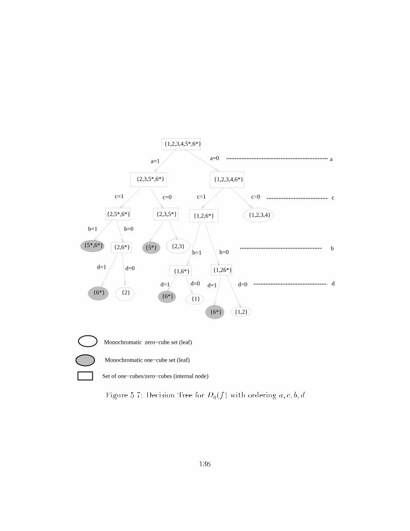
a=1 a=0
d=1 d=0
d=1 d=0 d=1 d=0 d
a
c
b
c=1 c=0 c=1 c=0
b=1 b=0
b=1 b=0
{1,2,3,4,5*,6*}
{2,3,5*,6*} {1,2,3,4,6*}
{2,5*,6*} {2,3,5*} {1,2,6*} {1,2,3,4}
{5*,6*} {2,6*} {5*} {2,3}
{6*} {2}{6*} {1}
{6*} {1,2}
{1,26*}{1,6*}
Monochromatic zero−cube set (leaf)
Monochromatic one−cube set (leaf)
Set of one−cubes/zero−cubes (internal node)
Figure ���� Decision Tree for D��f� with ordering a� c� b� d
���

a set of monochromatic cubes M where M � Cv and �Cv � O� � �Cv � Z��The permutation of indices generated by the the function � for each
variable in the input set I can be used to order the input variables� Thus inFigure ��� ��a� � � ��b� � � ��c� � � and ��d� � �� For convenience weshall denote the imposed ordering a � b � c � d by � � ha� b� c� di� Sinceinternal nodes in the decision tree are labeled with input variable names � Ithe ordering � also imposes a partial order � of levels l on the node set Vand the cube sets Cv associated with them� The levels in the node set aredistances from the leaves� The leaf nodes are at level � and the root nodeis at level n where n is the number of input variables j I j� This creates aset of ordered partitions of the node set V � fVn � Vn�� � � � � � V� � V�g�Each element of the partition is a set Vi consisting of all nodes at level i�Since each node v � Vi is associated with a cube set Cv we interchangeablyrefer to the elements of the set Vi as nodes �v� or cube sets �Cv�� We de�nea partition set PVi as the set consisting of the cube sets associated with eachnode in Vi� Therefore PVi � �v�ViCv� Thus a partition set PVi is a set ofsets� We can now de�ne a maximal partition set�
De�nition � Given a set of nodes Vi at level i� the maximal partition setPmaxVi
at this level is de�ned as
PmaxVi
� �v�ViCv such that �Cv � PmaxVi� iff Cv � Cw for w � Vi�
It contains all the cube sets in Vi such that no cube set is completely containedinside another� For every cube set Cv � Pmax
Vi the cube sets Cw that are
subsets of Cv are said to be covered by Cv�Before we look at an example we make one other observation� Since every
node v � Vi is labeled with the same input variable xj we can associate eachelement of the partition V � fVn � Vn�� � � � � � V� � V�g with a uniqueinput variable� This means we can rewrite Pmax
Vias Pmax
i�xj the maximal
partition set associated with an input variable xj � I at level i� in a decisiontree T �Dk� ��� To avoid confusion we shall adopt the convention of using thesubscript j for input variables and i for levels as far as possible�Let us now go back to the decision tree in Figure ���� The maximal
partition sets at each level i associated with each variable in � � ha� b� c� diare shown below�
Pmax��a � f��� �� �� �� ��� ���g
���

Pmax��b
� f��� �� ���� ��� �� �� �� ���gPmax��c
� f��� �� �� �� ���gPmax��d
� f��� �� ���gThe maximal partition set at a level consists of a set of cube sets at that
level� Every cube set in the maximal partition set has the characteristic thatthe subtree below it generates monochromatic leaf cube sets that are unique�i�e� not generated by any other element of the maximal partition set at thislevel� and maximal �i�e� it generates the largest possible monochromatic leafcube set��We now de�ne the signature S of a decision tree as follows�
De�nition The signature S of a decision tree T �Dk� �� is the union of themaximal partition sets associated with each input variable in the tree�
S � �xj�I
Pmaxi�xj
where i is the level associated with variable xj� The size of a signature j S jis the cardinality of the set S�The signature of a decision tree is a set of all the internal nodes that make
decisions to generate monochromatic cube sets at the leaves such that thecube set Cv associated with each such node v is unique and covers all othercube sets Cw that lie at the same level�The signature for the decision tree in Figure ��� is given by S �
f��� �� �� �� ��� ���� ��� �� ���� ��� �� �� �� ������ �� ���g and S � �Dk �Having introduced the decision tree we now return to the question ad
dressed at the beginning of this section� Rephrasing it we ask how can animplementation for a function be constructed given a decision tree T �Dk� ���Before we describe the procedure to construct this implementation some assumptions about our implementation model are necessary� We assume thatthe implementation is derived from a multilevel minimal expression representing a boolean function� The implementation assumes primitive technology mapping and uses only �input AND OR NOT gates corresponding tothe operators in the minimal expression of the function� A node in the implementation represents the output of a collection of gates that implement apartial function� The nesting depth in the minimal expression creates levels
���

in the implementation� Level � consists of the input literals and the levelsare numbered in increasing order moving from nodes �or partial functions�formed at the innermost level to the output node that has the maximumlevel number� Thus these levels impose a partial ordering on the nodes inthe implementation� Given a pair of nodes v�w belonging to levels i i� respectively if i i� then node v is closer to the inputs than node w� Theimplementation for the minimal expression
f � �c�a� b� � abd�
is shown in Figure ��� along with its partial functions�We now describe the procedure to construct an implementation from a
given decision tree T �Dk� ��� The procedure starts bottom up from the leaves�or monochromatic cube sets� of the tree� Using the ordering of the variablesspeci�ed by � the procedure examines the cube sets Cv associated with eachnode v at level i� Every cube set Cv at level i is replaced by a partial function
�f i�Cv� � xj��fi���childv�� � x�
j��f i���childv��
where xj is the input variable associated with the node v �f i���childv�� isthe partial function from the �child of v at level i� � and �f i���childv�� isthe partial function from the �child of v at level i� �� Since the childv� isa node where the value of xj � � and the childv� is a node where the valueof xj � � we can rewrite the partial function as
�f i � xj��fi��xj� x�
j��f i��x�
j�����
This is like the Shannon expansion of the function at level i except thatit is built bottom up from Shannon cofactors �with respect to xj� x�j� thatalready exist at the level below� The value of this partial function at any leveli is governed by a few rules� These rules are just manifestations of simpleboolean optimizations�
�� At the leaves of the tree �level �� there are only monochromatic onecube sets and monochromatic zerocube sets� If the leaf is a monochromatic onecube set then the partial function �f� has the value �� If theleaf is a monochromatic zerocube set then the partial function �f� hasthe value �� This corresponds to optimizations of the form x��� � x�
or x��� ��
���

a b c a b d
a.ba+b
(a+b).c a.b.d
c.(a+b)+abd
L=1
L=2
L=3
L=4
Figure ���� Implementation for f��c�a�b��abd�
���

�� For any level i � � suppose Cchildv�is the cube set at the onechild of
v and Cchildv�is the cube set at the zerochild of v� Then the partial
function �f i de�ned in Equation ��� can be reduced to
�f i � �f i��xj� x�
j��f i��x�j
provided c�� �c� � Cchildv�
� c� � Cchildv��
This says that if all the onecubes that belong to Cchildv�are contained
in Cchildv� then the literal xi is not making any useful decision and
hence is not part of the function� This corresponds to an optimizationof the form b� � bd � b� � d� Similarly if it is true that every �c� �Cchildv�
� � �c� � Cchildv�� then the partial function �f i reduces to
�f i � xj��fi��xj� �f i��x�
j
Here literal x�jis not making any useful decision in the tree and hence
does not appear in the partial function� The corresponding optimization is b� b�d� b� d�
�� For any level i � � if the cube set at the onechild of v Cchildv�is
identical to the cube set Cv at v then �f i � �f i��xj
If the cube set at
the zerochild of v Cchildv�is identical to the cube set Cv at v then
�f i � �f i��x�jThis performs the optimization b�cd � bcd � cd saying
that neither xj nor x�j are making any useful decisions�
�� For any level i � � if Cchildv�� Pmax
i���xkthen �f i can be reduced to
�f i � x�j��f i��x�
j
Similarly if Cchildv�� Pmax
i���xkthen �f i can be reduced to
�f i � xj��fi��xj
This says that if the cube sets at the onechild or zerochild of v arenot elements of the maximal partition set at that level then the partialfunctions associated with them can be ignored� Since there will be maximal partition set elements that covers these cube sets �Cchildv�
Cchildv��
the partial functions associated with these elements will cover �f i��x�j
and �f i��xj and hence they can be ignored here� This corresponds to
the optimization �ab� b�cd� � cd� �ab� cd��
���

In order to construct an implementation from the decision tree the partialfunctions computed at each level need to be replaced by gates� But our simple�input AND OR INVERTER gate model will not su�ce for this purpose�This is because the partial function constructed at a level may sometimesrequire more than one such primitive gate� This happens in two instances�
�� If every component of the partial function �f � x��fx�x���fx� is makinga contribution to the decision process then a pair of AND gates andan OR gate would be needed�
�� Similarly when the partial function is of the form �f � x��fx��fx� oneAND and one OR gate would be needed�
So we extend our implementation model to include a �input ANDOR gateAOR� and a �input ANDOR gate AOR�� Given that such complex gates doexist in practical implementations this extension does not seem unreasonable�We can now construct the implementation bottomup from the decision
tree by replacing the partial function at every node by a gate in the implementation� Thus the implementation is built incrementally� The set ofgates corresponding to the partial function at the root node is the multilevelimplementation of the entire function� The internal nodes in the implementation correspond to maximal partition sets in the decision tree at all levels� �� This is because it is only these nodes in the decision tree that contributeto the decision process and thus do not get optimized only during construction� The correspondence between input nodes in the implementation andinputs in the decision tree is di�cult to establish because of the decisiontree structure that forces the inputs to enter sequentially in contrast to animplementation where the inputs enter in parallel� So we shall restrict ourattention to the internal nodes of an implementation� Let us look at anexample�Figure ��� shows the cube space distribution for the function f � ac �
bc � abd implemented in Figure ���� It has � one zero cubes �not shown��The onecube set O and zerocube set Z in the minimum �decompositionare numbered below�
�� ac onecube�
�� bc onecube�
���

�� abd onecube�
�� c�d� zerocube�
�� b�c� zerocube�
�� a�b� zerocube�
�� a�c� zerocube�
Figure ���� shows the decision tree with the ordering � � hc� d� a� bi alongwith the constructed partial functions� Consider the nodes at the level �associated with d� For cube set f��� ��� ��� �g the partial function is computedas follows� Since the �child of this node has the same cube set f��� ��� ��� �gby rule � the partial function at this node is the same as the partial functionat its �child a�b� The partial function associated with the other cube set atlevel � f��� �� �� �� �g is computed as follows� Since the �child of this node isa monochromatic cube set rule � applies and �f i � xj�f i��xj
�f � d�ab� The
factored form representation of the function at the root node yields the multilevel implementation for this decision tree� The nodes in the implementationcorrespond to the partial functions at the maximal partition sets at each levelof the decision tree� Figure ���� illustrates the constructed implementation�
Since the implementation is derived from the decision tree a di�erentordering �� will possibly yield a di�erent decision tree and a di�erent implementation� Figure ���� illustrates this for the ordering �� � hd� c� a� b� i�Even though each ordering yields a di�erent decision tree the trees may besimilar in other respects� For instance we can de�ne cost�equivalent decisiontrees as follows�
De�nition Two decision trees T �D�f�� ���� T �D�f�� ��� have the samecost if their signatures S� and S� have the same sizes�
For the class of implementations that are derived from decision trees wecan state the following�
Lemma � If a pair of decision trees T �D�f�� ���� T �D�f�� ��� have the samecost� then the respective implementations I�� and I�� derived from them havethe same number of nodes�
���

a
b
c
d=0 d=1
a
b
c
f = ac+bc+abd
Figure ���� Cube Space Distribution for f � ac� bc� abd
���

AOR3
a b c a b d
a.ba+b
(a+b).c
a.b.d
c.(a+b)+abd
Figure ����� Implementation Constructed from Decision Tree in Figure ����
���

1*,2*,3*,4,5,6,7
1*,2*,3*,6 3*,4,5,6,7
1*,2*,3*,6 1*,2*,6 3*,5,6,7 4,5,6,7
1*,2*,3* 2*,6 1*,2* 2*,6 3*,5 5,6,7
6 6 52* 2* 3*
c=1 c=0
d=1 d=0 d=1 d=0
a=1 a=0 a=1a=0
a=1a=0
b=1 b=0 b=1 b=0 b=1 b=0
b
ab
abd
b
a+b
b
a+b
a+b
(a+b)c+abd
Monochromatic zero−cuboid set (leaf)
Monochromatic one−cuboid set (leaf)
Set of one−cuboids/zero−cuboids (internal node)
Figure ����� Decision Tree for f � ac� bc� abd with � � c� d� a� b
���
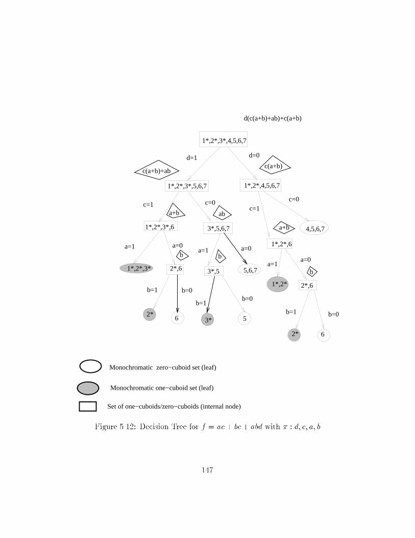
1*,2*,3*,4,5,6,7
1*,2*,3*,6
1*,2*,6
3*,5,6,7 4,5,6,7
1*,2*,3* 2*,6 3*,5 5,6,7
6 52*
3*
a=1 a=0a=1 a=0
b=1 b=0
b=0
b=1b=0
b
ab
a+b
b
a+b
1*,2* 2*,6
62*
a=1a=0
b=1
b
d=1 d=0
1*,2*,3*,5,6,7 1*,2*,4,5,6,7
c=1 c=0c=1
c=0
c(a+b)+ab
d(c(a+b)+ab)+c(a+b)
c(a+b)
Monochromatic zero−cuboid set (leaf)
Monochromatic one−cuboid set (leaf)
Set of one−cuboids/zero−cuboids (internal node)
Figure ����� Decision Tree for f � ac� bc� abd with � � d� c� a� b
���

Proof� By construction� Since the implementations are derived from thedecision tree the number of nodes in the implementation is equal to thenumber of maximal partition sets in the decision tree �by construction�� Sincethe decision trees have the same cost their signatures have the same numberof maximal partition sets and hence their implementations have the samenumber of nodes��
We now re�ne this cost measure between a pair of implementations �ordecision trees� to talk about costequivalence with respect to subtrees in apair of decision trees�Consider an ordering � � hxj� � � � � � xjni� By moving backwards in
the ordering we can create a series of partitions P �ithat are subsets of
the input variable set consistent with the ordering �� The �rst partition P �
� corresponds to ffxjng� fxjn��� � � � � xj�gg the second corresponds to
ffxjn � xjn��g� fxjn��
� � � � � xj�gg and so on until the last partition P �nequals
ffxjn � xjn��� � � � � x�g� fgg�
Consider two decision trees with orderings �� and �� such that �k whereP ��k � P ��
k � That is the subset of inputs in both these partitions is the sameeven though the order in which they entered their respective partitions maybe di�erent� The k in the partition P ��
k P ��k corresponds to the level k in the
implementation and is referred to as the join level�
De�nition �� Given a pair of partitions P ��k � P ��
k de�ned as above� withP ��k � P ��
k � their associated implementations I�� and I�� have the samecost with respect to this partition Pk if the total number of nodes in all thepartial functions in I�� is equal to the total number of nodes in all the partialfunctions in I�� computed till join level k�
In Figure ���� and Figure ���� the two implementations derived from therespective decision trees have the same cost with respect to the partitionffa� bg� fc� dgg of the input set fa� b� c� dg�We note that the partial functions at the join level k are functions of
variables in the set fxjk � � � � � xjng� They represent the cofactors of the originalfunction f with respect to the set fxj� � � � � � xjk��
g� Regardless of the order inwhich the inputs fxj�� � � � � xjk��
g were cofactored we would �nally arrive withthe same set of partial functions and the same number of maximal partitionsets at the join level�
���

Unfortunately our current notion of equivalence between implementations is much tighter than what we would ideally like� It needs to be expanded� If we can relax the assumption that identical partitions are neededat the join level it will help us derive a class of compatible implementationsat the join level giving us a broader notion of equivalence�
��� Spatial Entropy and Information Content
In the previous section we introduced the decision tree as an intermediate representation to relate a function with a broad class of implementations� Thetopdown reduction of the kdecomposition of the function into monochromatic cube sets generates the nodes and the leaves in the decision tree� Thebottomup construction of the kdecomposition from the leaves of the decision tree generates the implementation for the function�We have de�ned the information content I�f�Dk� of a function f in terms
of its kdecomposition Dk that appears at the root of all decision trees forf � In order to establish a relationship between the spatial entropy of animplementation of f and its information content I�f�Dk� we �rst de�ne thespatial entropy of a decision tree in terms of the onecubes and zerocubes inthe decision tree� Since a decision tree corresponds to an implementation wecan then relate this to the spatial entropy of an implementation as describedin Chapter ��The spatial entropy of an implementation was de�ned in Chapter � as the
dynamic communication e�ort required to compute a value �of � or �� for afunction� In the previous section we showed that the task of computing this�� or �� value is equivalent to the task of reducing the kdecomposition at theroot of the decision tree to the monochromatic cube sets at the leaves� Thepaths from the root to each leaf with a monochromatic onecube set describethe input onterms �� values� that belong to this onecube set� Similarly thepaths from the root to each leaf with a monochromatic zerocube set describethe o�terms �� values� that belong to this zerocube set� The e�ort requiredto generate all these monochromatic cube leaf sets from the root node is thespatial entropy of the decision tree�How can we express this e�ort formally� For this we use the notion of in
formation content de�ned in De�nition �� The spatial entropy of the decisiontree is the reduction in the information content I�f�Dk� of the function over
���

all the levels in the decision tree� At the root node I�froot�Dk� � I�f�Dk�which we reproduce below expresses the information content over the entirefunction�
I�f�Dk� �h
jOjjOj�jZj
� log��jOj�jZjjOj
�� jZj
jOj�jZj� log�
�jOj�jZjjZj
�i�hP
c��Ojc�j�n� log�
��n
jc�j
��P
c��Zjc�j�n� log�
��n
jc�j
�iAt the leaf node since there are only onecubes or only zerocubes the
�rst entropy function is � because either j O j or j Z j is � or the logexpression reducing to log��� equals �� As a result of this the informationcontent at a leaf node v I�fv�Dk� is �� At every level i � � in the decision treethe nodes v � Vi denote cofactors of the original function f with respect toall literal assignment�s� along the paths from the root to each of these nodes�We are only interested in those nodes whose cube sets Cv are elements of themaximal partition Pmax
i�xjat that level� This is because a cube set Cv � Pmax
i�xj
is a cube set whose one zerocube decomposition covers the one zerocubedecomposition of other cube sets that might appear at this level� Henceany decisions made with respect to this cube set would be a superset ofthe decisions made with respect to all the others it covers� For examplein Figure ��� �Page ���� the cube set f�� �� �� �� ��g � Pmax
��cat the level
corresponding to input variable c is a cube set that covers cube sets f�� �� ��gand f�� �� ��g� This node represents the cofactors of the function f � ab� cdwith respect to � literal assignments �a � �� b � �� �a � �� b � �� �a � �� b ��� all of which yield cd�Given that we are only interested in nodes v � Pmax
i�xjwe start by de�ning
the information content with respect to such a node v as
I�fv�Dk� �h
jOvjjOvj�jZvj
� log��jOvj�jZvj
jOvj
�� jZvj
jOvj�jZvj� log�
�jOvj�jZvj
jZvj
�i�hP
c��Ov
jc�j�n � log�
��n
jc�j
��P
c��Zvjc�j�n � log�
��n
jc�j
�iwhere Ov is the onecube set at v while Zv is the zerocube set at v� c�
is a onecube that belongs to Ov and c� is a zerocube that belongs to Zv�This de�nes the contribution of this node in making decisions to generate amonochromatic one zero cube set at the leaves� It also estimates the cost ofimplementing the partial function at this node its gatecount complexity�We use this de�nition to de�ne the cumulative information content at a
level i in the decision tree�
���

De�nition �� The cumulative information content I�fli�Dk� at a level i ina decision tree T �Dk� �� is de�ned as
I�fi�Dk� �X
Cv�Pmaxi�xj
I�fv�Dk�
where I�fv�Dk� is the information content with respect to a node that belongsto the maximal partition set at that level�
The cumulative information content at a level de�nes the gatecount complexity of the function f with respect to the inputs in the set fx�� � � � � xj��g � I�All the elements of the set fx�� � � � � xj��g precede xj in ��Going down the decision tree the change in information content from level
i to level i� � with a literal assignment xi or x�i tells us the contribution ofthat literal in reducing the information content� This is expressed as
%I�fi�Dk� � I�fi�Dk�� I�fi���Dk�
We are now ready to de�ne the spatial entropy of the decision tree�
De�nition �� The spatial entropy of a decision tree T �Dk� �� for a functionf with k�decomposition Dk and ordering � is
S�T �Dk� ��� �X
Pmaxi�xj
�S
%I�fi�Dk�
where� S is the signature of the decision tree� Pmaxi�xj
is a maximal partition
set � S at level i corresponding to variable xj in ��
We have thus expressed the e�ort required to generate monochromaticone zero cube sets at the leaves of a decision tree as a cumulative sum ofthe change in information content over the maximal partitions at each levelin the decision tree�We now try and relate the spatial entropy of an implementation as de
scribed in Chapter � to the spatial entropy of a decision tree� We use thefact that an implementation can be constructed bottomup from the decisiontree to establish this relationship� Since the decision tree representation doesnot capture wire length we assume that we are computing spatial entropyin the implementation with unit wire lengths� The monochromatic leaf cube
���

sets correspond to spatially distributed input sources in the implementation�Every node in the implementation denotes a partial function computed bythe implementation and corresponds to only those internal nodes in the decision tree whose cube sets belong to some maximal partition set� The rootnode which is the output of the implementation corresponds to the entirefunction� The e�ort required to reduce the kdecomposition at the root nodeto the monochromatic cube sets at the leaves can be expressed in reverse�On doing so we obtain the spatial entropy of an implementation� This is thee�ort required for the monochromatic leaf cube sets to combine with eachother while constructing the kdecomposition of the function�How can we express this e�ort formally� The spatial entropy of an imple
mentation can also be expressed using information content similar to way wede�ned the spatial entropy of a decision tree� We de�ne the spatial entropyof the implementation as the incremental contribution to the informationcontent I�f�Dk� of the function over all the nodes in the implementation�At the leaf nodes the information content is �� The root node expresses theinformation content over the entire function� Every internal node v in the implementation denotes a partial function� The information content I�fv�Dk�at this node v is computed from the cube set Cv� It indicates the e�ort contributed by the partial function at this node in combining the one zero cubesof the original function� The node!s contribution is computed by the increasein information content from the previous level in the implementation�Thus we can express the spatial entropy of an implementation I �con
structed from a decision tree T � using the expression
S�I�T �� �Xv�I
%I�fv�Dk�
where %I�fv�Dk� represents the increase in information content from onenode in the implementation to its immediate fanout node�
Lemma � The spatial entropy of an implementation constructed from adecision tree S�I�T �� is equal to the spatial entropy of a decision treeS�T ���Dk�� computed from the k�decomposition at the root�
Proof This is true by construction� The only nodes that contribute to thespatial entropy of a decision tree are nodes whose cube sets belong to themaximal partition� By construction every node in the implementation corresponds to a cube set belonging to some maximal partition� Hence the
���
contributions to the spatial entropy of the implementation and the decisiontree come from the same sources��
It should be noted that while a broad class of implementations can beconstructed from the decision tree they are restrictive in that they do nothave logical reconvergent fanout and technology mapping issues are ignored�We now turn our attention to the spatial entropy as we have de�ned it in
Chapter � to see how it relates to this de�nition� When a multilevel implementation is constructed for a function its kdecomposition is usually known�This is because the kdecomposition of the function corresponds to a minimal�irredundant prime� twolevel representation of a function� and multilevellogic minimization and synthesis often starts with such a minimized twolevel expression� We have seen that while computing the spatial entropy ofthe decision tree S�T ���Dk�� and while computing the spatial entropy of animplementation S�I�T �� from the decision tree we have knowledge of theonecubes and zerocubes and the function!s kdecomposition�On the other hand suppose we were interested in computing the spatial
entropy of an implementation that was already constructed� In such a caseits spatial entropy computation will have to be done without knowledge ofthe one zero cube distribution and the kdecomposition of the function� Thisis precisely what happens in the gatelevel spatial entropy computation procedure� In Chapter � we had de�ned the local spatial entropy at a node v asas�
�Sv �Xv��V
Hv � l�v�v��
where Hv is the information computed at the gate node v and l�v�v�� is thelength of the fanout edge from node v to v�� With a unit length assumption�Sv � Hv� Now let us look closely at the expression
Hv � p�vlog�
�
p�v
� � p�vlog�
�
p�v
�
p�vis the �probability of a node v and p�
vis the �probability of the node�
The � �or �� probability at the node is the fraction of onterms �or o�terms�in the cube space of the partial function being computed at the node�If we had used the expression for the information content at a node v in an
implementation derived from the decision tree we would have the expression
���
I�fv�Dk� de�ned earlier� The expression Hv is really an approximation tothe expression I�fv�Dk�� Let us see how� In a constructed implementationwe do not know the kdecomposition of the function� As a result we do notknow how the minterms of the partial function at each node contribute to theone zero cubes of the original function� So a simplistic assumption would beto assume that all the onterms of the partial function at that node contributeto the ON set of the function f and the all the o� terms contribute to theOFF set� This yields one big onecube and one big zerocube at the node�This means that j Ov j and j Zv j are � since there is only onecube and onezerocube� The expression I�fv�Dk� reduces to the following
I�fv�Dk� ��
����
� log������
�� �
���� log�
�����
����
jc�j�n log�
��n
jc�j
�� jc�j
�n log���n
jc�j
������ �
�� �
�jc�j�nlog�
��n
jc�j
�� jc�j
�nlog�
��n
jc�j
��
The size of the cubes j c� j and j c� j is equal to the number of mintermsin the cube� In j c� j this is the number of onterms while in j c� j this is thenumber of o�terms� So the expression jc�j
�nbecomes the �probability of the
node �p�v� and I�fv�Dk� reduced to Hv� AccumulatingHv over all the nodes
v � V yields the spatial entropy of the implementation�To summarize we began by de�ning the gatecount complexity of a
boolean function by its information content� We showed that the information content which is computed on a minimum kdecomposition of thefunction captures minimality in twolevel function representations� We thenshowed how a class of multilevel implementations for a given function couldbe derived from the decision tree representation� Minimality of multilevelimplementations was de�ned on the decision tree� We then de�ned the spatial entropy of an implementation computed bottomup from the decisiontree as the cumulative sum of the incremental information content over allthe corresponding nodes in the implementation� This gives a cube spacede�nition of spatial entropy that captures the communication between theminterms in the implementation� In the next section we verify empiricallythat the spatial entropy of an implementation tracks function behavior� Wealso show empirically that the information content and spatial entropy canbe used as estimates of the gatecount complexity of a function�
���

��� Experiment
The �rst objective of this experiment is to study the e�ectiveness of spatial entropy in measuring information content� Since information contentdepends on the minterm characteristics of the function this will tell us howe�ective spatial entropy is in capturing function behavior� As it may berecalled this was one of our objectives in establishing a theoretical basisfor using spatial entropy to generate BDD variable orders� Earlier in thischapter we de�ned an estimate for the gatecount complexity of a booleanfunction over a minimum k cube decomposition of the function� This estimate called the information content I�f�Dk� of the function was de�nedover cube characteristics that captured the gate cost in an implementation ofthe function� We then showed that the spatial entropy of an implementation�derived from a decision tree� can be de�ned as a function of the information content� Computing the spatial entropy of an implementation this wayis expensive because the size of a decision tree is exponential in the worstcase� In the previous section we also motivated the idea that the polynomialtime gate level spatial entropy computation of Chapter � could be used asan approximation to the spatial entropy computation over a decision tree�We verify this empirically in this experiment by using this polynomialtimeprocedure to measure information content� Our objective is to determine ifthere is su�cient correlation to use spatial entropy as a discriminator �ormeasure� of information content� For instance would we able to comparespatial entropies of a pair of functions and have the con�dence that we arecomparing their information content�In order to test our hypothesis we use the following criteria� We com
pute the sample correlation coe�cient r for the values of spatial entropy Sand information content I for a sample of circuits� �For convenience theinformation content expression I�f�Dk� is denoted as I�� The sample correlation coe�cient r which is a sample estimate of the population correlationcoe�cient is given by �Sto���
r �CISpCIICSS
r measures the degree of correlation between information content I and spatial entropy S� Values of r near �� indicate a strong positive correlationbetween S and I�S increases as I increases�� values of r near �� indicate
���

a strong negative correlation between S and I�S decreases as I increases��while if r � � then there is no correlation between S and I� We also determine the lines of regression �Sto��� of S on I and I on S� If there is perfectcorrelation r � �� then the two lines will coincide with each other and allthe experimental points will lie exactly on the common line of regression�For uncorrelated values the lines will be at right angles to each other�The second objective of this experiment is to study the e�ectiveness of
information content in estimating gate count complexity� As described earlier our de�nition of information content indicates minimality in twolevelfunctions� Since it captures cube characteristics that contribute to logic costwe would like to use it to estimate the gatecount complexity in a multilevelimplementation� To verify our hypothesis we use the same criteria as above�We compute the correlation coe�cient for information content I and gatecount GC for a sample of circuits where GC is the gate count in a technology mapped circuit implementation�
���� Assumptions
Our assumptions are along the lines of the quantities that we wish to compute spatial entropy �S� information content �I� and gatecount �GC�� Withrespect to spatial entropy computation our assumptions involve the threefactors discussed in Chapter �� redundancy wire length and reconvergentfanout� As mentioned in the previous section we would like to measure thespatial entropy on on a decision tree with the smallest signature size� Sincethis also corresponds to the spatial entropy of a minimized implementationwe assume redundancy is removed in the implementation by minimizing forliteral count� We use a unit wire length assumption for spatial entropy computation� This is because the de�nition of information content that we wishto track does not capture wiring complexity� In addition we have not beenable to explain the role of wire lengths in the decision tree representation�Finally we assume that errors in probabilities and spatial entropy due toreconvergent fanout are ignored�With respect to information content I we assume the following� Our es
timate is de�ned for singleoutput completely speci�ed functions� We ignorethe e�ect of don�t cares when functions are incompletely speci�ed� Sincewe have not de�ned information content for multioutput functions we currently use a naive approach� The information content of a multioutput
���

function is computed by computing the information content for a minimumkdecomposition of each of the outputs individually� So the information content I�f� for an moutput function would be computed as
I�f� �Xi���m
I�f�oi��Dk�oi��
This is actually an overestimate of the multioutput function!s complexitybecause the kdecompositions for each output function overlap �due to sharing of cube spaces between individual output functions�� Consequently theoverall information content would in most cases be less than the sum ofthe information contents of the individual functions� In order to remainconsistent in our comparisons when we compute the spatial entropy of suchmultioutput functions we use the cone�based approach �discussed in Chapter�� that computes the spatial entropy of each output function independently�Like the information content this too will be an overestimate of the spatialentropy of the multioutput function since the spatial entropy contributionof shared logic is not discounted�It was proved earlier in this chapter that the kdecomposition of a func
tion is equivalent to its twolevel prime irredundant representation� Sincecomputing the information content requires a kdecomposition of one zerocubes we use the output of a twolevel minimizer espresso �BHMSV��� togenerate these one zerocubes� The program espresso consists of a collection of heuristic algorithms for twolevel minimization and does not alwaysguarantee a minimum twolevel form� Thus for some functions our information content estimate does not use a minimum kdecomposition but anapproximately minimal kdecomposition�The gate count GC in an implementation is obtained by counting the
number of gates in a technology mapped multilevel implementation of thefunction� Like the assumption for spatial entropy we assume a minimized implementation while computing gate count� Since we compute the informationcontent for multioutput functions by computing the information content foreach function separately it would be inappropriate to compare this with thegate count in multioutput implementations� This is because multioutputfunctions share logic and the gate count in their implementations would be alot lesser than if they were implemented separately as singleoutput functions�So we compute gate count only only for single output implementations�
���

���� Data Set
The data set for the experiment is made up of two kinds of circuits bothdescribed as boolean functions in the PLA format �BHMSV���� The �rstset consists of several randomly generated singleoutput completely speci�ed boolean functions of �� �� �� �� � and � input variables� The number ofminterms in each of these functions and their positions in cube space wasrandomly generated� This data set satis�es the requirement of a wide rangeof boolean functions from � input functions to � input functions with di�erent cube sizes� Table ��� describes the characteristics of the �� � and � inputrandomly generated functions while Table ��� does the same for �� � and �input functions�The second set of data consists of twolevel boolean functions from the
MCNC Logic Synthesis �� benchmarks� This data set consists of singleoutput and multioutput functions some of which are incompletely speci�ed�These functions are shown in Table ���� The functions here are larger andmore irregular in their distribution of input output sizes minterm countand cube sizes� With this data set we get an opportunity to estimate andmeasure the complexity of boolean functions that have �presumably� usefulimplementations as against those of the randomly generated functions in the�rst data set set�In the �rst part of the experiment we determine the spatial entropy mea
sure S information content estimate I and the gate count GC for � samplesets of randomly generated functions with varying input sizes extractedfrom the data sets in Table ��� and Table ���� Each sample of �� functionsis made up of a uniform mix of �� �� �� �� � and � input functions� This givesus � separate data sets on which to correlate spatial entropy and informationcontent� In the second part of the experiment we generate spatial entropy information content and gate count for the the Logic Synthesis �� benchmarkcircuits�
�� Experiment Outline
Figure ���� shows the software construction and the experiment outline forcomputing the information content I for each function and the spatial entropy S and gate count GC for a minimized implementation� Computing
���

Circuit Product One ZeroName Inputs Terms Cubes Cubesf� � � �� � �f� � � � � �f� � � � � �f� � � �� � �f� � � �� � �f� � � � � �f� � � � � �f� � � �� � �f� � � � � �f� �� � � � �f� � � �� �� �f� � � �� � �f� � � �� � �f� � � � � �f� � � � � �f� � � �� � �f� � � �� � �f� � � �� � �f� � � �� � �f� �� � �� �� �f� � � �� �� ��f� � � �� �� ��f� � � �� �� ��f� � � �� �� ��f� � � �� �� ��f� � � �� �� ��f� � � �� � �f� � � �� � ��f� � � �� �� �f� �� � �� �� ��
Table ���� �� and � input randomly generated functions
���

Circuit Product One ZeroName Inputs Terms Cubes Cubesf� � � �� �� ��f� � � �� �� ��f� � � �� �� ��f� � � ��� �� ��f� � � �� �� ��f� � � �� �� ��f� � � �� �� ��f� � � �� �� ��f� � � �� �� ��f� �� � ��� �� ��f� � � �� �� ��f� � � ��� �� ��f� � � �� �� ��f� � � ��� �� ��f� � � ��� �� ��f� � � ��� �� �f� � � ��� �� ��f� � � ��� �� ��f� � � �� �� ��f� �� � ��� �� ��f� � � ��� �� ��f� � � ��� �� ��f� � � ��� �� ��f� � � ��� �� ��f� � � ��� �� ��f� � � �� �� ��f� � � ��� �� ��f� � � ��� �� ��f� � � ��� �� ��f� �� � ��� �� ��
Table ���� �� and � input randomly generated functions
���
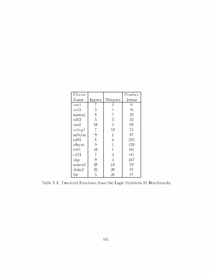
Circuit ProductName Inputs Outputs Termscon� � � �xor� � � ��misex� � � ��rd�� � � ��sao� �� � ��m�xp� � �� ��m�sym � � ��rd�� � � ���z�sym � � ���t��� �� � ���rd�� � � ���clip � � ���misex� �� �� ��duke� �� �� ��bw � �� ��
Table ���� Twolevel Functions from the Logic Synthesis �� Benchmarks
���
the information content estimate requires measuring the following variables�number of onterms o�terms number of one zero cubes and sizes of one zerocubes� As the �gure indicates each PLA representation is minimized at thetwolevel for its ON set and OFF set to obtain the one zero cube set thatmakes up the kdecomposition� This is then used to compute the information content measure� The spatial entropy S is computed along the linesof the experiment in Chapter �� First the twolevel PLA representation isminimized via SIS �BRSVW��� and a multilevel technology mapped implementation in VPNR �KB��� is generated� This is then used by the spatialentropy computation program spent to generate spatial entropy measures�The spatial entropy measures for both the ON and OFF set implementationsof the PLA are obtained and the lesser of the two is selected� This is becausewe are interested in the spatial entropy of a minimized implementation andthere are several occasions where implementing a function as its OFF set� inverted� yields an implementation with lesser spatial entropy� Since themultilevel minimization program SIS does not always detect this scenariowe perform this task explicitly�The spatial entropy of an implementation is computed with unit wire
length and no reconvergent fanout removal� On encountering multiple fanoutnodes the spatial entropy is divided equally amongst the fanout nodes� Thisensures that the overall spatial entropy is preserved when fanout nodes reconverge� The gate count GC is computed from the VPNR implementations�The information content for multioutput functions is calculated by com
puting the on o� terms and the one zerocubes for each individual outputfunctions by factoring out the common cubes� These values of I�foi� are thenaccumulated over all the output functions foi The spatial entropy for multioutput functions is calculated in two steps� In the �rst step the logic cone foreach output function foi is computed by traversing backward from the output oi� This determines the logic that contributes to the output function foi�The spatial entropy Sfoi with respect to this cone is then calculated� Afterperforming this task over all output functions the spatial entropy values overall cones are accumulated to obtain the spatial entropy of the multioutputfunction Sf � For m outputs we have
Sf �Xi���m
Sfoi
���

PLA Input
SISMulti−level Minimization
espressoGenerate D k
VPNR Netlist
spent gen_infcontent
Spatial Entropy (S) Information Content (I(f,D ))k
GateCount(GC)
One−cubesZero−cubes
Figure ����� Experiment Outline
���

��� Results and Observations
���� Results
Tables ��� ��� and ��� illustrate the results of spatial entropy gatecount and information content for three sets of randomly generated functions� Table ��� tabulates spatial entropy and information content for theLogic Synthesis �� benchmarks� As mentioned earlier the gate count wasnot computed for these implementations since they are multioutput implementations that share logic while the information content computation doesnot assume sharing� The spatial entropy measures shown here are obtainedafter computing the spatial entropy for minimized implementations of theONset and the OFFset and then taking the lesser of the two� The gatecount is obtained similarly�
���� Observations
Table ��� �page ���� shows the mean and variance of spatial entropy andinformation content values for the random function data sets and the LogicSynthesis �� benchmarks� We observe that the variance of the random function �for both spatial entropy and information content� is not as high as itis for the benchmark circuits� This is because the benchmark circuits are farmore diverse with a wider range of features� The individual functions aremuch further apart from each other in terms of their complexity and information content� There are functions with inputs ranging from � to �� andoutputs ranging from � to ���The other observation that we make with respect to the spatial entropy
and information content is that spatial entropy values show a higher variance than the information content values for all data sets� The reason forthis is that the implementations of two functions can di�er in a lot moreways than the speci�cations of the same two functions� There are a lot morevariables involved gates gate types their connectivity and arrangementetc� probabilities when spatial entropy is being computed at the implementation level� On the other hand the information content is computed on thefunction speci�cation in terms a few �xed variables� So �uctuations are lessdrastic�We study correlation between spatial entropy and information content
���

Circuit GateName Inputs S I�f�DK� Countf� � � ����� ���� �f� � � ���� ���� �f� � � ���� ���� ��f� � � ����� ����� ��f� � � ����� ����� ��f� � � ����� ���� �f� � � ����� ����� ��f� � � ����� ����� ��f� � � ����� ����� ��f� � � ����� ����� ��f� � � ����� ����� ��f� � � ����� ����� ��f� �� � ����� ����� ��f� � � ����� ����� ���f� � � ����� ����� ���f� �� � ����� ����� ��f� � � ����� ����� ���f� � � ����� ����� ���f� � � ������ ����� ���
Table ���� S I�f�Dk� and GC for random circuits �Set ��
���

Circuit GateName Inputs S I�f�DK� Countf� � � ����� ���� �f� � � ����� ����� ��f� � � ����� ����� �f� � � ����� ���� ��f� � � ����� ����� ��f� � � ���� ���� �f� � � ����� ����� ��f� � � ����� ����� ��f� � � ����� ����� ��f� �� � ����� ����� ��f� � � ����� ����� ��f� � � ������ ����� ��f� � � ����� ����� ��f� � � ����� ����� ���f� � � ����� ����� ���f� � � ����� ����� ���f� � � ����� ����� ���f� � � ����� ����� ���f� �� � ����� ����� ���
Table ���� S I�f�Dk� and GC for random circuits �Set ��
���

Circuit GateName Inputs S I�f�DK� Countf� �� � ����� ����� ��f� � � ����� ���� ��f� � � ����� ���� ��f� � � ����� ���� ��f� � � ����� ����� ��f� � � ����� ���� ��f� � � ����� ����� ��f� � � ������ ����� ��f� � � ������ ����� ��f� � � ����� ����� ��f� � � ����� ����� ��f� � � ����� ����� ��f� � � ����� ����� ��f� � � ����� ����� ��f� � � ���� ����� ���f� � � ����� ����� ���f� � � ����� ����� ���f� � � ����� ����� ���f� � � ����� ����� ���
Table ���� S I�f�Dk� and GC for random circuits �Set ��
���

CircuitName S I�f�DK�con� ������ ������xor� ����� ���misex� ������ ������rd�� ����� ������sao� ������� ������m�xp� ������� ������m�sym ����� ������rd�� ������ ������z�sym ������ ������t��� ����� ������rd�� ������ �������clip ������ ������misex� ������ ������duke� ������ �������bw ������ �������
Table ���� Spatial Entropy and Information Content for Logic Synthesis ��benchmarks
Data Spatial Entropy �S� Information Content �I�Set Mean Variance Mean Variance
Random Set � ����� ������ ���� ����Random Set � ����� ������ ���� ����Random Set � ����� ������ ���� ����
LgSynt�� Benchmarks ������ ��������� ����� �������
Table ���� Mean and Variance of Spatial Entropy �S� and Information Content �I�
���
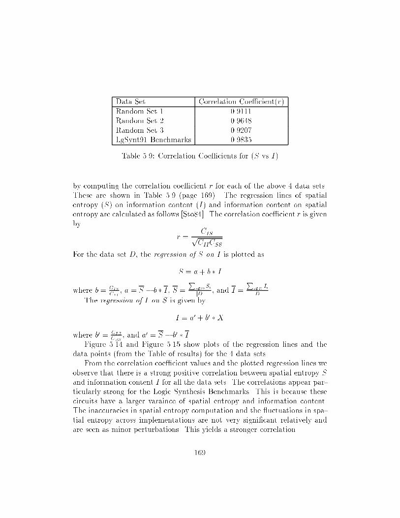
Data Set Correlation Coe�cient�r�Random Set � ������Random Set � ������Random Set � ������LgSynt�� Benchmarks ������
Table ���� Correlation Coe�cients for �S vs I�
by computing the correlation coe�cient r for each of the above � data sets�These are shown in Table ��� �page ����� The regression lines of spatialentropy �S� on information content �I� and information content on spatialentropy are calculated as follows �Sto���� The correlation coe�cient r is givenby
r �CISpCIICSS
For the data set D the regression of S on I is plotted as
S � a� b � I
where b � CIS
CII a � S � b � I S �
Pi�D
Si
jDj and I �
Pi�D
Ii
jDj�
The regression of I on S is given by
I � a� � b� �X
where b� � CIS
CSS and a� � S � b� � I�
Figure ���� and Figure ���� show plots of the regression lines and thedata points �from the Table of results� for the � data sets�From the correlation coe�cient values and the plotted regression lines we
observe that there is a strong positive correlation between spatial entropy Sand information content I for all the data sets� The correlations appear particularly strong for the Logic Synthesis Benchmarks� This is because thesecircuits have a larger varaince of spatial entropy and information content�The inaccuracies in spatial entropy computation and the �uctuations in spatial entropy across implementations are not very signi�cant relatively andare seen as minor perturbations� This yields a stronger correlation�
���

��
��
��
�
��
�
�
� � � � � � ��
SpatialEntropy
S
Information Content I
Random Set ��I vs S�
Correlation Coe�cient r � ������
regression line of S on Iregression line of I on S
�I�S� values �
����
� �
�
�
�
�
��
�
��
�
�
��
��
��
��
�
��
�
�
� � � � � � ��
SpatialEntropy
S
Information Content I
Random Set ��I vs S�
Correlation Coe�cient r � ������
regression line of S on Iregression line of I on S
�I�S� values �
���
���
����
�
��
� �
�
�
�
�
Figure ����� Regression Lines and Data plots �S vs I�
���

��
��
��
�
��
�
�
� � � � � � ��
SpatialEntropy
S
Information Content I
Random Set ��I vs S�
Correlation Coe�cient r � ������
regression line of S on Iregression line of I on S
�I�S� values �
�� ��� � �
��
�
���
�
��
���
���
���
���
��
���
��
�� �� � ��� ��� ���
SpatialEntropy
S
Information Content I
Logic Synthesis � Benchmarks
Correlation Coe�cient r � ������
regression line of S on Iregression line of I on S
�I�S� values �
�����
���� �
���
�
�
Figure ����� Regression Lines and Data plots �S vs I�
���

Data Set Correlation Coe�cient�r�Random Set � �����Random Set � �����Random Set � �����
Table ����� Correlation Coe�cients for �GC vs I�
The average value of the correlation coe�cient over the � random datasets is ������ indicating a strong correlation� This is inspite of the fact thatthe random functions have a much lesser variance in information content�This lesser variance would normally make it more di�cult to discriminatebetween information contents of di�erent functions� But this correlationshows that spatial entropy is capable of measuring information content evenin such functions�We now study the correlation between information content and gate
count� Table ���� �page ���� shows the correlation coe�cient r for the threerandom data sets� The plots are shown in Figure ���� �page ���� and Figure ���� �page �����The correlation coe�cient values and the regression lines indicate a de�
nite positive correlation between information content and gate count thoughit is not as strong as the correlation between information content and spatial entropy� This tells us that information content is a good estimate ofgatecount complexity in boolean functions� Some of the �uctuations can beexplained by the fact that we have used a gate count measure obtained after technology mapping� A more accurate physical attribute like active areamight have helped since it takes into account the di�erence in area occupiedbetween complex gates and simpler gates�The fact that there is a high correlation between information content I
and spatial entropy S suggests that there might be a positive correlation between spatial entropy S and gate count GC in a multilevel implementation�We study this by computing the correlation coe�cient r for spatial entropyand gate count for the three random data sets� These are shown in Table �����page ����� The regression line plots are shown in Figure ���� �page ����and Figure �����page �����We notice that there is high degree of correlation between gate count and
���
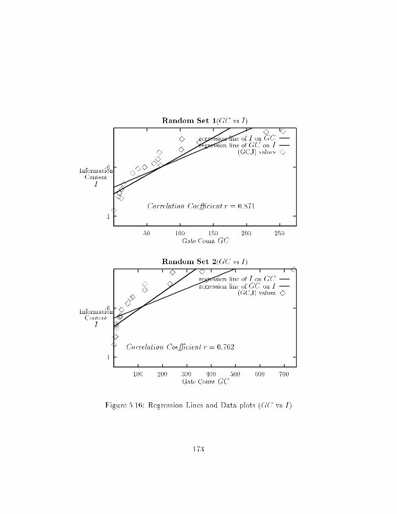
�
�� ��� ��� ��� ���
InformationContent
I
Gate Count GC
Random Set ��GC vs I�
Correlation Coe�cient r � �����
regression line of I on GCregression line of GC on I
�GC�I� values �
�
��
��
�
���
����
�
�
�
�
��
�
��� ��� ��� �� ��� �� ��
InformationContent
I
Gate Count GC
Random Set ��GC vs I�
Correlation Coe�cient r � �����
regression line of I on GCregression line of GC on I
�GC�I� values �
�
�
�
��
�
����
���
���
���
Figure ����� Regression Lines and Data plots �GC vs I�
���

�
��� ��� ��� �� ��� �� ��
InformationContent
I
Gate Count GC
Random Set ��GC vs I�
Correlation Coe�cient r � �����
regression line of I on GCregression line of GC on I
�GC�I� values �
�
��
�
��
��
�
����
�
��
�� �
Figure ����� Regression Lines and Data plots �GC vs I�
Data Set Correlation Coe�cient�r�Random Set � �����Random Set � ����Random Set � �����
Table ����� Correlation Coe�cients for � data sets �Gate Count vs S�
���

��
��
��
�
��
�
�
�� ��� ��� ��� ���
SpatialEntropy
S
Gate Count GC
Random Set ��GC vs S�
Correlation Coe�cient r � �����
regression line of S on GCregression line of GC on S
�GC�S� values �
�
�����
�
�
�
�
�
�
�
�
�
�
�
�
�
��
��
��
�
��
�
�
��� ��� ��� �� ��� �� ��
SpatialEntropy
S
Gate Count GC
Random Set ��GC vs S�
Correlation Coe�cient r � ����
regression line of S on GCregression line of GC on S
�GC�S� values �
��
�
���
����
��
�
�
��
�
�
�
Figure ����� Regression Lines and Data plots �GC vs S�
���

��
��
��
�
��
�
�
��� ��� ��� �� ��� �� ��
SpatialEntropy
S
Gate Count GC
Random Set ��GC vs S�
Correlation Coe�cient r � �����
regression line of S on GCregression line of GC on S
�GC�S� values �
���
�����
�
���
�
���
���
Figure ����� Regression Lines and Data plots �GC vs S�
spatial entropy for all the data sets� Thus spatial entropy gives us a measureof circuit area� In earlier chapters we explained how spatial entropy capturesthe switching energy in an implementation� How do these two relate� Giventhat we limit our scope to only combinational circuits the switching energy inthese circuits is a function of the switching of �� �� states at the nodes and theswitching delays at the nodes in the implementation� In most combinationalcircuits this switching energy is equivalent to the circuit area since almostthe entire circuit switches while the circuit computes� This explains the highcorrelation between spatial entropy and circuit area measured by gate count�
��� Conclusions
From the experimental results of the previous section we can conclude thatspatial entropy is a good measure for the information content of the function�Even when the functions are much closer in cube space as in the case ofthe random data sets we observe that there is strong positive correlation�������� between spatial entropy and information content� In Chapter � westudied the use of spatial entropy for variable ordering of BDDs� We observed
���

that due to the sensitivity of the BDD construction process and the �negranularity of usage of the spatial entropy attribute �individual contributionsin a spatial entropy vector� approximations and inaccuracies in the spatialentropy computation were quite signi�cant� This in turn had an adversee�ect on the resultant orderings and BDD sizes� In this chapter we observethat since we did not have to deal with sensitivity and spatial entropy valuesat such a �ne level the approximations in spatial entropy computation didnot a�ect the quality of the solution� This is an important observation� Itinforms us that while the results of applying spatial entropy may not be asrewarding in one case they might be a lot better in another�The information content of a function is a characteristic of the function
and its cube space distribution independent of the myriad of implementations that might be generated to compute this function� The fact that thespatial entropy computed on a minimized implementation of the function iscapable of measuring such a characteristic makes it a very useful measureto study functions over an entire class of implementations� This lends morecredence to our work in Chapter � on using spatial entropy for BDD variableordering and provides empirical evidence that there is some basis to usingspatial entropy for BDD variable ordering� The decision tree for a given input ordering can be very easily transformed into a BDD for that ordering� itis quite likely that this might yield a more formal relationship between BDDsizes and spatial entropy� We intend to pursue work in this direction�We can also conclude that information content our de�nition of gate
count complexity does estimate logic gate cost well� We observed a de�nitepositive correlation between information content an abstract attribute de�ned in cube space and the gate count obtained from the implementation�The high correlation between spatial entropy and information content showedthat it too can be used to estimate circuit area� Since we have not been ableestimate wiring at the cube space level wiring complexity is not captured inour results� Variances in cube sizes was not modeled in our de�nition of information content neither did we use any kind of distance length informationwhile de�ning the spatial entropy of the decision tree or computing spatialentropy on a gate level implementation in the experiments� The variance incube sizes a�ects the distance cubes need to travel before getting combinedand this might have an in�uence on the wiring factor� The recent work onusing lexicographic ordering �PAS�� ASSP��� to minimize the routing factorin multilevel synthesis further supports this� We elaborate on this brie�y�
���
In their research Saucier et�al adopt a lexicographic factorization strategy to generate the multilevel factored form of a function and show thatthis strategy reduces wiring complexity in the layout� A lexicographic factorization generates factors for a function all of which are compatible witha reference order on the input variables� For example the factors ab�ce� d�and ce�d�f� are compatible with the reference order b � a � c � e � d f �This idea can be related to the decision tree and its nodes� The factors
and their subfactors are partial functions at the cube sets that are membersof maximal partition sets in a decision tree� The reference order determinesthe ordering of variables in the decision tree�Suppose we had two decision trees built on two orderings where one of
the orderings is a reference order for a lexicographic factorization� The number of nodes in the decision tree built with lexicographic factorization willbe lesser than the the number of nodes in the decision tree built withoutlexicographic factorization� The reference order for the lexicographic factorization generates compatible factors� These factors correspond to nodesor cube sets that make independent decisions about generating monochromatic one zerocubes� For example in the factor ab�ce�d� with the orderingb a c e d the path a � �� b � � will immediately yield a monochromatic zerocube set at the level corresponding to c� Meanwhile all the othera� b combinations will yield exactly one cube set belonging to a maximal partition set at the level corresponding to c� Now the factor �ce � d� can actindependently to generate its monochromatic zero cube set for c � �� e � �at level c and below� Thus several cube sets in the decision tree get mergedinto maximal partition sets yielding decision trees with lesser nodes� Anordering like b e d a c will not be able to achieve such similarsharing� This implies larger nodes due to more number of maximal partitionsets� A formal treatment of this with the spatial entropy expressions at thenodes of the decision tree could yield some useful results with respect towiring complexity� The fact that the lexicographic factorization strategy hasalso been used to generate BDD variable orders further indicates a possiblefundamental relationship between spatial entropy and BDD sizes�
���

Chapter �
Conclusions
In this dissertation we have introduced spatial entropy to the VLSI domainas an attribute that captures the dynamic communication e�ort in a circuit�Its quantitative de�nition uni�es static structure and dynamic usage in acircuit� In a physical implementation �for CMOS circuits� this de�nitionis a good model for measuring the switching energy in a circuit� We haveshown how to compute spatial entropy at di�erent levels of abstraction andhave characterized it in extensive detail� We illustrated its use by applyingit to a CAD problem that has traditionally relied on static attribute basedsolutions� We also showed that it can be used to capture function behaviorthrough implementations�
��� Summary
There are several problems in CAD where function behavior needs to becaptured through an implementation� Using static attributes computed fromthe topology of the implementation is not always helpful for this purpose�Firstly they do not provide su�cient usage information and secondly theytend to exhibit variances with implementations which is not desirable whilecapturing function behavior� There is also a need for an attribute that canunify behavior and structure in order to answer questions about the functionand the implementation�We have introduced a circuit attribute capable of meeting some of these
requirements using a concept called spatial entropy� Intuitively it is the dy

namic communication e�ort �or work done� in the circuit while computingthe underlying function� We have de�ned the attribute quantitatively usingthe entropy function from information theory� This de�nition is computableat di�erent levels of abstraction and it uni�es the static structure and dynamic usage in a circuit� On a physical �CMOS� implementation spatialentropy computes the switching energy in a circuit� This quanti�es the intuitive notion of spatial entropy in the form of a physical attribute that is ofrelevance to designers�It is di�cult to compute spatial entropy accurately� The levels of ab
straction hide information needed to compute it and other factors like reconvergent fanout a�ect its accuracy� On applying spatial entropy to theproblem of generating variable orders in BDDs we found that it performscompetitively with earlier static attribute based approaches� But as circuitsget larger the inaccuracies in computing spatial entropy have a signi�cante�ect on the quality of the solution�We have shown that spatial entropy is capable of capturing function be
havior through an implementation� An implementation with minimum spatial entropy has minimum switching energy and describes the minimum communication e�ort required to compute the function� Such an implementationis like a signature for the function since its measures of spatial entropy �andswitching energy� provide a lower bound over all implementations of thatfunction� Since it is di�cult compute a minimal spatial entropy implementation we approximate it by using a minimal gate count implementationand show that the spatial entropy computed on such an implementation cancapture function behavior� We characterize function behavior by de�ninginformation content the gatecount complexity of a function in cube space�We then show that there is a strong correlation between the spatial entropyof a minimal gate count implementation and the information content of afunction� Moreover inaccuracies in spatial entropy computation do not havethe signi�cant e�ect they had in BDD variable ordering� There is also empirical evidence that information content �in cube space� is a good estimatorof actual gatecount complexity�What can we conclude about spatial entropy!s role in CAD from this
research� The empirical evidence that spatial entropy tracks function behavior suggests that there is a fundamental basis for using spatial entropyto generate BDD variable orders� A BDD is strictly a characteristic of thefunction and its minterms� A decision tree for a function depends on its
���

input variable ordering� and it is easy to transform one into a BDD for thatordering� The cube space de�nition of spatial entropy over a decision treegives us a mechanism for distinguishing one tree �or BDD� from another andconsequently one ordering from another� This can give us a theoretical basisfor connecting spatial entropy and variable ordering�The quantitative de�nition of spatial entropy provides a good model for
switching energy in a physical implementation� Switching energy and dynamic power consumption are of concern to every designer� and spatial entropy provides a quantitative comparison of these measures between di�erentcircuit implementations� Generating a minimumspatial entropy implementation is a desirable goal for a designer since minimum spatial entropy impliesminimum switching energy� But existing synthesis and layout tools that generate physical implementations are incapable of generating implementationswith minimum spatial entropy since they are unable to minimize wires alongwith logic gates� Minimizing wires is also of concern in performance drivenlogic and layout synthesis and minimum spatial entropy can become a usefulmetric of performance in these areas too�Depending on the level of abstraction �boolean function gate or layout�
at which the implementation is viewed there are di�erent interpretations tospatial entropy� in all of them spatial entropy captures a notion of dynamice�ort� For an implementation denoted by a multilevel function it is theincremental contribution in cube space to compute the information contentof the function� For an implementation denoted by a gate level netlist itis the information �ow computed as the informationdistance product overall the nodes in the implementation� For an implementation at the physicallayout level it models the switching energy in the implementation� Thisindicates the generic applicability of the spatial entropy concept�While trying to track function behavior from a gate level implementation
we observed that spatial entropy can be e�ciently computed but computingit accurately is a di�cult task� This inaccuracy in spatial entropy computation can a�ect some problems �BDD variable ordering� more than others�measuring gatecount complexity�� The primary drawback here is poor estimates of wire length at the gate level� This lack of wiring informationis also tied in to the goal of achieving minimum spatial entropy� An implementation with minimum spatial entropy is di�cult to achieve currentlybecause existing logic synthesis tools only minimize for gate count ignoringwire length information� Since we could not capture wiring estimates in the
���

form of variances in cubes sizes in our information content de�nition wecould not extend our estimate of gatecount complexity to include wiringcomplexity� Improved estimates of wire length will not only help us do thisbut also achieve minimal spatial entropy implementations and more accuratemeasures of spatial entropy at the gate level�
��� Future Research Directions
As discussed above using decision trees to demonstrate that there is a theoretical basis for using spatial entropy for BDD variable ordering is one of themore immediate problems that has spawned from this research� The problemof estimating wiring complexity at the cube space level and using it to re�nethe information content de�nition I�f�Dk� is another issue that has directrelevance�In addition to these issues we see spatial entropy being applicable in other
areas of CAD primarily those where static structure and dynamic usage cantogether provide more information to solve a problem� A partial list of theseareas is discussed below�
Spatial Entropy for Logic Synthesis� Logic synthesis involves severalphases that repeatedly make areatime tradeo� decisions� At almostevery stage in the synthesis process when data is needed in two di�erent places at the same time the logic computing it needs to be reused�The issue then is� should it be replicated �recomputed� at the desiredlocation or should it be factored out and transmitted �via a fanout orwire� to the desired location� Spatial entropy can capture the areatimetradeo� in this decision elegantly� We have seen that the wire lengthsin spatial entropy computation can provide a measure of dynamic communication e�ort by modeling the distance traveled by information� Atthe same time they can also be used to model the wiring complexity ina circuit to study trade o�s in circuit area minimization� Using spatialentropy �along with an active area measure� to control the extractionof kernel intersections during logic synthesis could lead to a new metricto measure the quality of synthesized circuits that captures active areaand the wiring area�
Device��tting� The logicwire unifying property of spatial entropy and its
���
ability to measure function complexity can also help address problemsin device �tting software design for FPGA and PLDs� The softwarethat maps twolevel logic equations into complex cells in FPGAs andPLDs has to tackle problems of design partitioning via boolean functiondecomposition minimization and technology mapping followed by signal place and route� These are quite often iterative tasks where literalcomplexity and wiring complexity trade o� with each other� Spatialentropy could be used as a cost measure here to assist in global decisions�
Design Space Parsing� Spatial entropy is currently being used as a toolto perform high level designspace parsing and exploration �Tya��a��The designspace of di�erent areatime implementations of datapathfunctions can be characterized into primitive models on the basis ofthe communication pattern exhibited by these functions� Due to similar communication behavior the spatial entropy values for di�erentareatime implementations of these functions will show a similar distribution� This structures the task of design space exploration�
State Transition Graph Discrimination� The distribution of spatial entropy values at the outputs of a sequential circuit helps discriminatethe structure of state transition graphs� This is useful information foralgorithms that perform state machine traversal during sequential circuit veri�cation and test generation since it gives an indication of thegraph structure� whether it is deep or shallow broad or narrow� Thisin turn can help state transition graph traversal algorithms�
���

Bibliography
�Agr��� V� Agrawal� An Information Theoretic Approach to DigitalFault Testing� IEEE Transactions on Computers pages ���&��� August �����
�Ake��� S� B� Akers� Binary Decision Diagrams� IEEE Transactions onComputers C���������&��� June �����
�AS��� K� J� Antreich and M� H� Schulz� Accelerated Fault Simulationand Fault Grading in Combinational Circuits� IEEE Transac�tions on Computer�Aided�Design CAD��������&��� September �����
�ASSP��� P� Abouzeid K� Sakouti G� Saucier and F� Poirot� MultilevelSynthesis minimizing the routing factor� In ��th ACM�IEEEDesign Automation Conference pages ���&��� June �����
�BA��� H� Bouzouzou and P� Abouzeid� Personal Communication�MCNC Logic Synthesis �� Benchmarks BDD Orderings May�����
�BBR��� K� S� Brace R� E� Bryant and R� L� Rudell� E�cient Implementation of a BDD Package� In Proceedings of the ��thACM�IEEE Design Automation Conference June �����
�Ber��� C� Leonard Berman� Circuit Width Register Allocation andOrdered Binary Decision Diagrams� IEEE Transactions onComputer�Aided�Design CAD����������&���� August �����
�BHMSV��� R� K� Brayton G� Hatchel C� McMullen and A� SangiovanniVincentelli� Logic Minimization Algorithms for VLSI Synthesis�Kluwer Academic Press� Boston �����
�BI��� D� Brand and V� S� Iyengar� Timing Analysis uusing FunctionalRelationship� In IEEE ICCAD ��� Digest of Technical Paperspages ���&��� November �����
�BM��� R� K� Brayton and C� McMullen� The Decomposition and Factorization of Boolean Expressions� In International Symposiumon Circuits and Systems pages ��&�� May �����
�BMCM��� J� Benkoski E� V� Meersch L� J� M� Claesen and H� D� Man�Timing Veri�cation using Statically Sensitizable Paths� IEEETransactions on Computer�Aided�Design CAD����������&���� October �����
�BPH��� Franc� Brglez P� Pownall and R� Hum� Applications of Testability Analysis� In Proceedings of the IEEE International TestConference pages ���&��� �����
�Bra��� K� Brace� Personal Communication� BDD Orderings June�����
�BRM��� K� M� Butler D� E� Ross and M� R� Mercer� Heuristics to Compute Variable Orderings for E�cient Manipulation of OrderedBinary Decision Diagrams� In Proceedings of the IEEE�ACMDesign Automation Conference pages ���&��� June �����
�BRSVW��� R� K� Brayton R� Rudell A� SangiovaniVincentelli andA� Wang� MIS� A MultipleLevel Logic Optimization System� IEEE Transactions on CAD CAD������&���� November �����
�Bry��� R� E� Bryant� Graph based algorithms for Boolean functionmanipulation� IEEE Transactions on Computers C���������&��� August �����
�Bry��� R� E� Bryant� On the Complexity of VLSI implementations andGraph Representations of Boolean functions with applications
���

to Integer Multiplication� IEEE Transactions on ComputersC���������&��� Feb �����
�CA��� KT Cheng and V� D� Agrawal� An Entropy Measure forthe Complexity of MultiOutput Boolean Functions� In ��thACM�IEEE Design Automation Conference pages ���&���June �����
�CF��� R� W� Cook and M� J� Flynn� Logical Network Cost andEntropy� IEEE Transactions on Computers C������&���September �����
�Dus��� J� Dussault� A Testability Measure� In Proceedings of the ���Semiconductor Test Conference pages ���&��� October �����
�DYG��� D� H� C� Du S� H� C� Yen and S� Ghanta� On the GeneralFalse Path Problem in Timing Analysis� In Proceedings of the��th IEEE�ACM Design Automation Conference �����
�FFK��� M� Fujita H� Fujisawa and N� Kawato� Evaluation and improvements of Boolean comparison method based on binarydecision diagrams� In Proceedings of the IEEE InternationalConference on Computer�Aided Design November �����
�FMK��� M� Fujita Y� Matsunaga and T� Kakuda� On variable orderingof Binary Decision Diagrams for the application of multilevellogic synthesis� In Proceedings of the European Conference onDesign Automation pages ��&�� February �����
�FS��� S� J� Friedman and K� J� Supowit� Finding the Optimal VariableOrdering for Binary Decision Diagrams� IEEE Transactions onComputers C���������&��� May �����
�GJ��� M� R� Garey and D� S� Johnson� Computers and Intractability�A Guide to the Theory of NP�Completeness� Freeman Press�New York �����
�Hel��� L� Hellerman� AMeasure of Computational Work� IEEE Trans�actions on Computers C������&��� May �����
���

�HM��� K�S� Hwang and M� R� Mercer� Derivation and Re�nement ofFanout Constraints to Generate Tests in Combinational LogicCircuits� IEEE Transactions on Computer�Aided Design CAD�����&��� October �����
�HOI��� T� Hwang R� M� Owens and M� J� Irwin� CommunicationComplexity Driven Logic Synthesis� In Proceedings of the ���International Workshop on Logic Synthesis �����
�HOI��� T�T� Hwang R� M� Owens and M� J� Irwin� E�ciently Computing Communication Complexity for Multilevel Logic Synthesis� IEEE Transactions on Computer�Aided Design ������&��� May �����
�ISY��� N� Ishiura H� Sawada and S� Yajima� Minimization of BinaryDecision Diagrams based on Exchange of Variables� In Proceed�ings of the International Conference of Computer�Aided Designpages ���&��� November �����
�JA��� S� K� Jain and V�D� Agrawal� STAFAN� An Alternative toFault Simulation� In Proceedings of the � st Design AutomationConference pages ��&�� �����
�JPHS��� S� W� Jeong B� Plessier G� D� Hatchel and F� Somenzi� Variable ordering for FSM Traversal� In International Workshop onLogic Synthesis May �����
�Kap��� R� Kapur� Personal Communication� BDD Orderings for acollection of heuristics July �����
�KB��� G� Kedem and F� Brglez� OASIS� Open Architecture SiliconImplementation System� Technical Report TR���� Microelectronics Center of North Carolina Feb �����
�Kel��� E� Kellerman� A Formula for Logical Network Cost� IEEETransactions on Computers C������&��� September �����
�Koh��� Z� Kohavi� Switching and Finite A Auto Theory� McGrawHill�����
���

�Koo��� G� Koob� An abstract Complexity Theory for Boolean Func�tions� University of Illinois at UrbanaChampaign �����
�Law��� E� J� Lawler� An Approach to Multilevel Boolean Minimization�Journal of the ACM pages ���&��� �����
�LBdGG��� R� Lisanke F� Brglez Aaart J� de Geus and David Gregory� TestabilityDriven Random Test Pattern Generation� IEEE Transactions on Computer�Aided Design CAD���������&���� November �����
�LBK��� R� Lisanke F� Brglez and G� Kedem� McMAP� A Fast Technology Mapping Procedure for MultiLevel Logic Synthesis� InProceedings of the IEEE International Conference on ComputerDesign October �����
�Lee��� C� Y� Lee� Representation of switching circuits by Binary Decision Programs� Bell Systems Technical Journal ������&���July �����
�LKB��� R� Lisanke G� Kedem and F� Brglez� DECAF� Decomposition and Factoring for MultiLevel Logic Synthesis� TechnicalReport TR���� Microelectronics Center of North CarolinaAugust �����
�LP��� M� Lorenzetti and B� Preas� Physical Design Automationof VLSI Systems� BenjaminCummings Publishing Company�����
�Mas��� K� Mase� Comments on �A Measure of Computational Work�and �Logical Network Cost and Entropy�� IEEE Transactionson Computers C�����&�� January �����
�MC��� C� Mead and L� Conway� Introduction to VLSI Systems chapterPhysics of Computational Systems pages ���&���� AddisonWesley Publishing Company �����
�McC��� E�J� McCluskey� Introduction to the Theory of Switching Cir�cuits� McGrawHill �����
���

�Min��� S�I Minato� Personal Communication� BDD Orderings usingminimum width method for ISCAS�� and Logic Synthesis ��Benchmarks May �����
�MIY��� S�I� Minato N� Ishiura and S� Yajima� Shared Binary DecisionDiagram with Attributed Edges for e�cient Boolean functionmanipulation� In Proceedings of the IEEE�ACM Design Au�tomation Conference pages ��&�� November �����
�MJ��� F� Maamari and J�Rajski� A Method of Fault Simulation basedon Stem Regions� IEEE Transactions on Computer�Aided De�sign CAD�����&��� February �����
�MK��� P� C� McGeer and R� K�Brayton� E�cient Algorithms for Computing the Longest Viable Path in a Combinational Network�In Proceedings of the ��th Design Automation Conference June�����
�MKR��� M� Ray Mercer R� Kapur and D� E� Ross� Functional Approaches to Generate Orderings for E�cient Symbolic Representations� In Proceedings of the ��th ACM�IEEE Design Au�tomation Conference pages ���&��� June �����
�Mul��� D� E� Muller� Complexity in Electronice Switching Circuits�IRE Transactions on Electron� Comput� EC����&�� Mar�����
�MWBV��� S� Malik A� R� Wang R� K� Brayton and A� S� Vincentelli�Logic Veri�cation using Binary Decision Diagrams in a LogicSynthesis Environment� In Proceedings of the IEEE Interna�tional Conference on Computer�Aided Design November �����
�Ous��� J� K� Ousterhout� Crystal� A Timing Analyzer for nMOS VLSICircuits� In Proceedings of �rd Caltech Conference on VLSI�Computer Science Press �����
�PAS��� F� Poirot P� Abouzeid and G� Saucier� Lexicographic Factorizations minimizing the critical path and the routing factor� InIFIP Working Conference on Logic and Architecture SynthesisJune �����
���
�PCD��� S� Perremans L� Claesen and H� DeMan� Static Timing Analysis of Dynamically Sensitizable Paths� In Proceedings of the��th Design Automation Conference June �����
�Pip��� N� Pippenger� Information Theory and the Complexity ofBoolean Functions� Mathematical Systems Theory ������&��������
�PM��� K� P� Parker and E� J� McCluskey� Probabilistic Treatmentof General Combinational Networks� IEEE Transactions onComputers C������&��� June �����
�RBKM��� D� E� Ross K� M� Butler R� Kapur and M� R� Mercer� FastFunctional Evaluation of Candidate OBDD Variable Orderings�In Proceedings of the European Conference on Design Automa�tion pages �&�� February �����
�Ree��� D� Reeves� Personal Communication� vpnr�bdd informationJuly �����
�Ris��� R� H� Risch� Staggered Input Networks� An Approach to Automatic Logic Decomposition� In Proceedings of the InternationalSymposium on Circuits and Systems pages ��&�� �����
�RT��� A� Rajanala and A� Tyagi� A New AreaBased Figure of Meritfor Layout Synthesis Systems� In Proceedings of the ��� Inter�national Workshop on Layout Synthesis� MCNC ACM SIGDAMay �����
�Sau��� G� Saucier� Analysis of the Trends in Logic Synthesis� In Pro�ceedings of the Synthesis and Simulation Meeting and Interna�tional Interchange SASIMI pages �&�� April �����
�SB��� M� Schulz and Franc Brglez� Accelerated TransitionFault Simulation� In Proceedings of the ��th Design Automation Confer�ence pages ���&��� �����
�SDB��� J� Savir G� S� Ditlow and P� H� Bardell� Random PatternTestability� IEEE Transactions on Computers C�����&��January �����
���

�Sea��� F� W� Sears� Thermodynamics� the kinetic theory of gases� andstatistical mechanics� AddisonWesley Publishing CompanyInc� �����
�Sha��� C� E� Shannon� The Synthesis of Twoterminal Switching Circuits� Bell Systems Technical Journal pages ��&�� January�����
�SPA��� S� C� Seth L� Pan and V� D� Agrawal� PREDICT� ProbabilisticEstimation of Digital Circuit Testability� In Proceedings of the �th Annual Symposium on Fault�Tolerant Computing pages���&��� �����
�Sto��� K� Stoodley� Applied and Computational Statistics� EllisHorwood Limited �����
�SW��� C� E� Shannon and W� Weaver� The mathematical theory ofcommunication� The University of Illinois Press� Urbana �����
�TA��� K� Thearling and J� Abraham� An easily computed FunctionalLevel Testability Measure� In Proceedings of the ��� Interna�tional Test Conference pages ���&��� �����
�Tho��� C� D� Thompson� Areatime Complexity for VLSI� In Pro�ceedings of the th Annual ACM Symposium on the Theory ofComputing pages ��&�� �����
�TSB��� H� J� Touati H� Savoj and R� Brayton� Delay Optimizationof Combinational Logic Circuits through Clustering and Partial Collapsing� In Proceedings of the IEEE International Con�ference on Computer�Aided Design pages ���&��� November�����
�Tya��a� A� Tyagi� An Algebraic Model for Datapath designspace exploration� In International Workshop on Formal Methods inVLSI Design January �����
�Tya��b� A� Tyagi� How Many Paths Classify a Function� A Study in Design Space Extraction� In Proceedings of the ��th InternationalSymposium on Circuits and Systems� IEEE June �����
���

�Yao��� A� C� Yao� Some Complexity Questions Related to DistributedComputing� In Proceedings of ACM Symposium on Theory ofComputing pages ���&��� �����
���