HEADING CONTROL OF AN UNDERWATER VEHICLE

SURAJ MISHRA (108EE032)

KARANKI DINESH (108EE041)

Department of Electrical Engineering

National Institute of Technology Rourkela

HEADING CONTROL OF AN UNDERWATER VEHICLE

a thesis submitted in partial fulfillment of the requirements for the degree of

Bachelor of Technology in Electrical Engineering

By

Suraj Mishra (108EE032)

Karanki Dinesh (108EE041)

Department of Electrical Engineering

National Institute of Technology

Rourkela

HEADING CONTROL OF AN UNDERWATER VEHICLE

a thesis submitted in partial fulfillment of the requirements for the degree of

Bachelor of Technology in Electrical Engineering

By

Suraj Mishra (108EE032)

Karanki Dinesh (108EE041)

under the guidance of

Prof. Bidyadhar Subudhi

Department of Electrical Engineering

National Institute of Technology

Rourkela

 

 

NATIONAL INSTITUTE OF TECHNOLOGY ROURKELA

CERTIFICATE

This is to certify that the thesis entitled “Heading Control of an Underwater Vehicle”

submitted by Suraj Mishra and Karanki Dinesh in partial fulfillment of the requirements for

the award of Bachelor of Technology Degree in Electrical Engineering at the National

Institute of Technology, Rourkela, is an authentic work carried out by them under my

supervision.

To the best of my knowledge the matter embodied in the thesis has not been submitted to any

other University/Institute for the award of any degree or diploma

Date: Prof. Bidyadhar Subudhi

Department of Electrical Engineering

National Institute of Technology

Rourkela-769008, Odisha

 

v  

ACKNOWLEDGEMENT

No thesis is created entirely by an individual, many people have helped to create this thesis and

each of their contribution has been valuable. Our deepest gratitude goes to our thesis supervisor,

Prof. Bidyadhar Subudhi, Department of Electrical Engineering, for his guidance, support,

motivation and encouragement throughout the period this work was carried out. His readiness for

consultation at all times, his educative comments, his concern and assistance even with practical

things have been invaluable. We would also like to thank all professors and lecturers, and

members of the department of Electrical Engineering for their generous help in various ways for

the completion of this thesis.

Karanki Dinesh Suraj Mishra

Roll no. 108EE041 Roll no. 108EE032

Dept. of Electrical Engineering Dept. of Electrical Engineering

NIT Rourkela NIT Rourkela

 

 

vi  

 

ABSTRACT

In this thesis an overview of Autonomous Underwater Vehicles (AUV) is presented which

covers the state of art in AUV technology, different components such as sensors and actuators of

AUV and the applications of AUVs. This thesis describes the development and verification of

six degree of freedom, non-linear simulation model. In this model, external forces and moments

are defined in terms of vehicle coefficients. A nonlinear model of AUV is obtained through

kinematics and dynamics equations which are linearized about an operating point to get a

linearized horizontal plane model. The objective of the AUV control here is heading control i.e.

to generate appropriate rudder angle position and thrust so that the desired heading is achieved.

For the above heading control we develop a controller that consists of two loops, one is

controlled by a PD controller and the other loop by a P control action. The first and second order

Nomoto model of the vehicle is formulated and studied for simpler qualitative analysis of

complicated ship model.

Simulation studies were undertaken also for yaw control of a single AUV. The above controller

is designed for effective tracking of desired trajectory of the AUV in horizontal plane. All the

simulations were performed using both MATLAB and SIMULINK.

The results obtained for heading and yaw control of the AUV studied are presented and

discussed in this thesis.

 

vii  

CONTENTS  

ABSTRACT vi 

TABLE OF CONTENTS vii

LIST OF TABLES ix

LIST OF FIGURES ix

CHAPTER 1: Introduction 1

1.1 Background of an AUV 1

1.2 Applications of AUVs 2

1.3 State of art 3

1.4 Main components of an AUV 4

1.4.1 Sensors and actuators 6

1.5 Objectives of the Thesis 7

1.6 Organisation the Thesis 8

CHAPTER 2:Kinamatics and Dynamics of an AUV 9

2.1 Coordinate frame assignment 9

2.2 Kinmatics 10

2.3 Dynamics 12

2.4 Linearized kinematics and dynamics 13

2.5 Steering controller 14

2.6 Linearized coefficent derivation 15

2.6.1 Hydrostatics 15

2.6.2 Hydrodynamic damping 15

2.6.3 Added mass 18

2.6.4 Fin lift forces and moments 19

 

viii  

2.6.5 Body lift forces and moments 20

2.6.6 Combined terms 21

2.7 SIMULINK model 23

2.8 Results and discussion 24

2.9 MATLAB Code 28

2.10 Summary 30

CHAPTER 3:Heading control of underwater vehicle 31

3.1 Nomoto model of AUV 31

3.2 Nomoto model analysis using SIMULINK 34

3.3 Summary 39

CHAPTER 4: Path tracking of an AUV 40

4.1 Error Dynamics 40

4.2 Simulation result 41

4.2 MATLAB code 42

CHAPTER 5:Conclusion 46

REFERENCES 47

 

 

ix  

LIST OF TABLES:

Table 2.1: Notation used in AUV modeling 9

Table 2.2:Linearized vehicle Coefficents 21

LIST OF FIGURES: 

Fig 1.1 : Components of an AUV 4

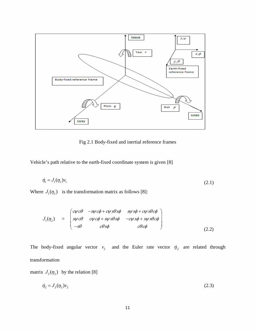
Fig 2.1 : Body-fixed and inertial reference frames 11

Fig 2.2 : SIMULINK model with fin angle saturation 23

Fig 2.3 : yaw angle ~ time 24

Fig 2.4 : y ~ time 25

Fig 2.5 : des ~ time 25 Fig 2.6 : R ~ time 26

Fig 2.7 : error in Y ~ time 27

Fig 2.8 : error in ~ time 27

Fig 2.9 : Dynamics simulation of the AUV 28 Fig 3.1 : SIMULINK model of 2nd order Nomoto model 34

Fig 3.2 : Bode plot of 1st order Nomoto model for heading control of an AUV 35 Fig 3.3 : Step response of 1st order Nomoto model for heading control of an AUV 35 Fig 3.4 : Bode plot of 2nd order Nomoto model for heading control of an AUV 36 Fig 3.5 : Step response of 2nd order Nomoto model for heading control of an AUV 36 Fig 3.6 : Root locus of 2nd order Nomoto model for heading control of an AUV 37 Fig 3.7 : Bode plot of 2nd order Nomoto model for heading control of an AUV 38 Fig 3.8 : Step response of 2nd order Nomoto model for heading control of an AUV 38 Fig 3.9 : Root locus of 2nd order Nomoto model for heading control of an AUV 39

 

x  

Fig 4.1 : Tracking control of AUV in horizontal plane 41

Fig 4.2 : Trajectory tracking of two thruster model 43

 

1  

CHAPTER 1:

INTRODUCTION

With the development of technology and applied sciences, the remotely operated vehicle (ROV)

industry has made itself well established with thousands of ROVs having been assembled and

deployed. The need for control and automation in robots, however, is becoming a more dominant

issue in many situations and environmental conditions. One of the major deciding factor whether

a vehicle is to be designed as an ROV or as an autonomous vehicle is its ability to communicate

with the operator. Autonomous control is preferred to remote control in environments where

communication with a vehicle is constrained.

One of the environments in which communication is inhibited is underwater. Underwater robots

are playing a major role in underwater expedition and in exploring greater depths. Assembled

and specialized vehicles for deepwater missions have been used in the offshore industry since

late 1960s. However excessive dependence on a communications tether and a control platform

has restricted their applications.

1.1 AUTONOMOUS UNDERWATER VEHICLE

Due to these limitations of ROVs there has been a surge in interest towards AUVs. AUVs are

fully automatic and submersible platforms capable of performing underwater tasks and missions

with their onboard sensor, navigation and payload equipments [6].The reason for this surge is

many scientific and commercial tasks involve hazardous and inaccessible environments which

can be performed by AUVs without any human guidance. The development of AUVs has been

 

2  

boosted by advancement in material science, sophisticated digital control and extremely accurate

sensors. Present research on AUVs focuses on making them more compatible, automatic and

intelligent. With an aim of achieving the above said goals, thorough research is going on

worldwide with high priority on navigation, autonomy and control.

1.2 APPLICATIONS OF AUVs

Due to technical constraints, AUVs were engaged in limited tasks and missions but with rapid

enhancement in technology nowadays AUVs are being deployed for many critical jobs with

persistently evolving roles and missions.

i. Commercial: Most of the oil and gas industry requires sea floor mapping and

surveying before developing infrastructure. Nowadays AUVs are the most cost

effective solution for this job with minimum environmental interference. With the

help of AUVs we have an upper hand over the traditional bathymetric technique.

Also post-lay pipeline surveys are now possible.

ii. Military: Incorporating its sonar technology AUVs are capable of detecting manned

submarines in anti-submarine warfare. They are also used to locate mines and detect

unidentified objects to secure an area.

iii. Research: To explore the ocean floor and microscopic lives in it scientist use AUVs

equipped with special sensors for their detection and study.

iv. Environment: For long term monitoring of radiation levels, leakage, pollution in

aquatic habitats and inspection of underwater structures such as dams, pipelines and

dykes AUVs are being utilized.

 

3  

1.3 STATE OF ART

From the beginning human beings have always desired to explore the unexplored. This crave has

empowered men to throw light on what lies deep down under sea. Due to physical limitations

from the beginning automatic vehicles are preferred for deep sea exploration. The first Special

Purpose Underwater Research Vehicle was developed by Stan Murphy and Bob Francois at the

Applied Physics Laboratory at the University of Washington in 1957.

In the 1970s, first AUVs were built and they were put into commercial use in the 1990s. Today

AUVs are mostly used for scientific studies, commercial purposes, military and survey

operations. The HUGIN series was developed in cooperation between Kongsberg Maritime and

the Norwegian Defense Research Establishment and it is the most commercially successful AUV

series on the world market today.[1]

Challenges, now an AUV faces are navigation, communication, autonomy, and endurance issues.

Automatic functioning is an important aspect of AUVs which deals with circuit configuration

and controller strategy. In this project work, the main concern is on the autonomy. During a

mission, an AUV may undergo different steering scenarios such as a complete turn at the end of

a trajectory, a severe roll during avoiding an obstacle or frequent depth changes while following

a tough seabed terrain. Different operations demand different controller strategy. A yaw and

surge controller is used to guide the AUV on a particular direction without changing depth. A

tracking controller is used to move the AUV on a predefined path.

 

4  

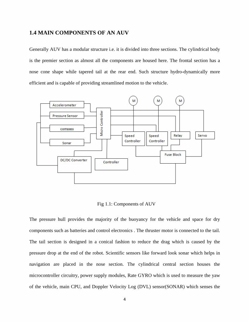
1.4 MAIN COMPONENTS OF AN AUV

Generally AUV has a modular structure i.e. it is divided into three sections. The cylindrical body

is the premier section as almost all the components are housed here. The frontal section has a

nose cone shape while tapered tail at the rear end. Such structure hydro-dynamically more

efficient and is capable of providing streamlined motion to the vehicle.

Fig 1.1: Components of AUV

The pressure hull provides the majority of the buoyancy for the vehicle and space for dry

components such as batteries and control electronics . The thruster motor is connected to the tail.

The tail section is designed in a conical fashion to reduce the drag which is caused by the

pressure drop at the end of the robot. Scientific sensors like forward look sonar which helps in

navigation are placed in the nose section. The cylindrical central section houses the

microcontroller circuitry, power supply modules, Rate GYRO which is used to measure the yaw

of the vehicle, main CPU, and Doppler Velocity Log (DVL) sensor(SONAR) which senses the

 

5  

approximate distance travelled in direction of each coordinate axis. Fins help in changing the

depth attained by vehicle. Rudder is movable vertically mounted fin, and performs the control of

heading direction of the vehicle. Thruster motor is provided at stern end to provide necessary

torque to move the vehicle in forward direction and rudder fins control the heading.

POWER MODULE

Pressure tolerant batteries are preferred for AUV. These special batteries do not require a special

housing chamber for them. This eliminates the risk of fire hazard due to explosion of battery. the

more deeper we go inside the water, the more pressure we are likely to observe. The pressure

tolerant design provides better energy and strength to the battery.

GPS

Global Positioning System is a satellite navigation system maintained by the US government,

which provides location and time information in all weather condition. With the help of GPS we

can get the exact co-ordinates of any object and can locate it anywhere on the earth. To realize

track following algorithm, coordinates of the vehicle must be determined precisely, which is

provided by the GPS system.

SONAR

Sound Navigation and Ranging (SONAR) is a method that uses sound waves as a medium to

navigate, communicate and detect objects in its path. In subsea environments it is very important

to avoid collision with static obstacles which is done with the help of SONAR. The sound waves

 

6  

sent from AUV are reflected back by obstacle and these signals are received by AUV to detect

presence of object.

DOPPLER VELOCITY LOG

To provide navigation information Doppler Velocity Log (DVL) is used. DVL exploits

Doppler’s effect to calculate the velocity of the robot. By bouncing sound frequency in a

direction it can determine the velocity of the vehicle in that direction. DVL is also quite useful in

determining absolute displacement relative to a fixed frame.

INERTIAL MEASUREMENT UNIT

Inertial Measurement Unit (IMU) uses Gyroscope and Accelerometer to determine the velocity,

orientation and the net gravitational force on the AUV. Using dead reckoning technique, the

computer keeps a track of the AUV using the data obtained from the IMU. The Gyro being an

integral member of the inertial navigational unit, helps in measuring and maintaining the

orientation of the vehicle. Accelerometer provides data on velocity of the vehicle

1.4.1 SENSORS AND ACTUATORS

Different types of sensors are used depending upon the application of AUV e.g. whether we want

to know the temperature of water, depth of seabed, concentration of any substance present or

high quality photos for study.

TEMPERATURE SENSORS: Generally Platinum Resistance Thermometers (PRTs), which

are suitable for use in all conditions, are used. PRTs and thermistors are both used for calculating

any temperature level.

 

7  

PRESSURE SENSORS: Strain gauge type pressure sensors are sensitive to temperature

variation and hence the data obtained varies with all temperature level, irrespective of the

extreme temperature. By the inclusion of a temperature sensor which is diffused into the silicon

of the strain sensor, this problem can be overcome. The thermal characterization of the

completed sensor is then obtained, which allows a performance of better accuracy over the full

working range of temperatures.

CONDUCTIVITY SENSORS: It uses an epoxy formed body linked to a stainless steel base for

standard applications.

OPTICAL SENSORS: Sensors such as transmisometers and fluorimeters operate by emitting a

light beam (pulsed for the fluorimeters) through optical filters and into the sea water via a

window set in the face of the sensor housing which has to be relatively thick to withstand high

pressures. [5]

1.5 OBJECTIVES OF THE THESIS

The objectives of this project were to:

design and model a prototype of the vehicle

contrive a new control strategy for the vehicle

Design a controller for track following of vehicle in 2D.

This project work was divided into two phases. First phase deals with modeling of the vehicle

while the second phase deals with its controller design. This report doesn’t deal with practical

implementation as it deals only with theoretical realization.

 

8  

1.6 ORGANISATION OF THESIS

This thesis is divided into five chapters.

Chapter 2, throws some light on the fundamental theories and concepts regarding underwater

vehicles and their design. A brief discussion on kinematics and dynamics of the vehicle is given.

The linearized model of the vehicle is considered and its linearized coefficients are calculated. Then a

SIMULINK model of the vehicle is studied.

Chapter 3, presents an approximated NOMOTO model of the vehicle which is used for simpler

heading control. The 1st and 2nd order model is studied along with their stabilizations. PD

controller is used for stabilization of the model with optimum settling time and overshoot

limitations.

Chapter 4, introduces the concept of error dynamics, which is optimally reduced for track

following of the vehicle. The track following of an AUV is shown along with its MATLAB

code. Trajectory tracking of a two thruster model is also shown using PD and LQR control

technique.

 

   

 

 

 

9  

CHAPTER 2:

KINEMATICS AND DYNAMICS OF AN AUV

To design any, vehicle knowledge of physical laws governing the system is essential. In this

chapter modeling and design of AUV in horizontal plane is examined. Controller design of AUV

using simple P-PD controller is presented. SIMULINK model for the system is designed and

results are obtained to check stability of the obtained system.

2.1 COORDINATE FRAME ASSIGNMENT

To study the motion of marine vehicle 6 degrees of freedom are required since to describe

independently the complete position and orientation of the vehicle we require 6 independent

coordinates. To describe position and translation motion first three sets of coordinates and their

time derivatives are required. While for orientation and rotational motion last three sets of

coordinates and their time derivatives are required.

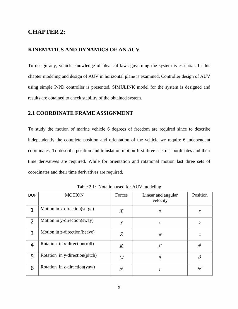
Table 2.1: Notation used for AUV modeling

DOF  MOTION Forces Linear and angular velocity 

Position

1  Motion in x-direction(surge)  X   u    x   

2  Motion in y-direction(sway)  Y   v    y

3  Motion in z-direction(heave)  Z   w    z   

4  Rotation in x-direction(roll)  K   p

5  Rotation in y-direction(pitch) M   q  

6  Rotation in z-direction(yaw)  N   r   

 

10  

 

To obtain a mathematical model of the AUV, its study can be divided into two sub-categories:

Kinematics and Dynamics.

Kinematics deals with bodies at rest or moving with constant velocity whereas dynamics deals

with bodies having accelerated motion.

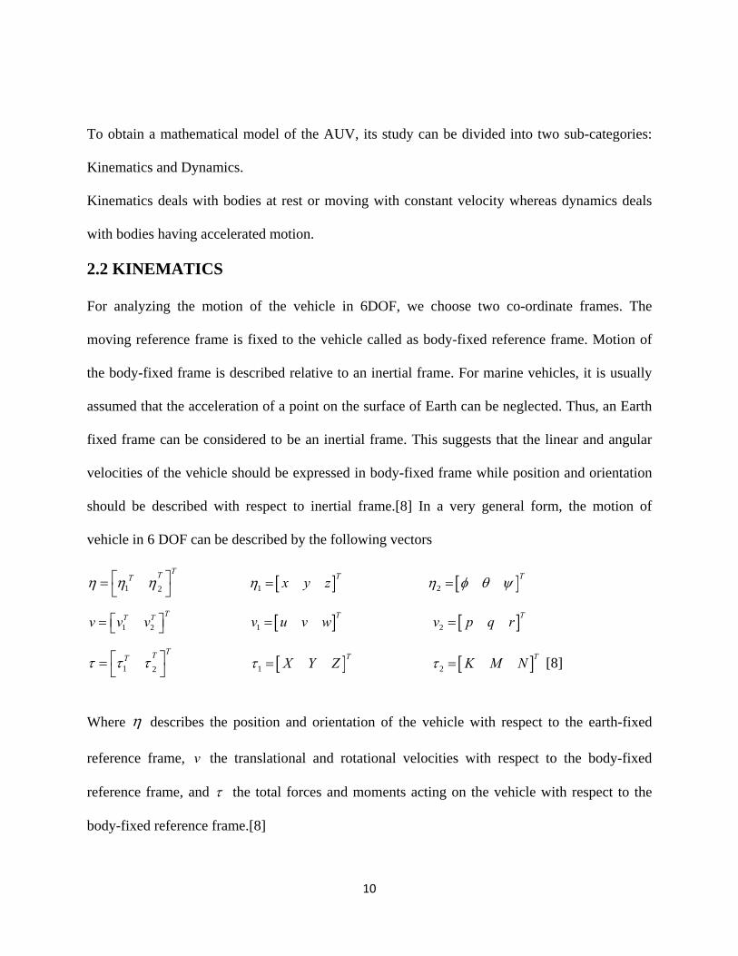
2.2 KINEMATICS

For analyzing the motion of the vehicle in 6DOF, we choose two co-ordinate frames. The

moving reference frame is fixed to the vehicle called as body-fixed reference frame. Motion of

the body-fixed frame is described relative to an inertial frame. For marine vehicles, it is usually

assumed that the acceleration of a point on the surface of Earth can be neglected. Thus, an Earth

fixed frame can be considered to be an inertial frame. This suggests that the linear and angular

velocities of the vehicle should be expressed in body-fixed frame while position and orientation

should be described with respect to inertial frame.[8] In a very general form, the motion of

vehicle in 6 DOF can be described by the following vectors

1 2

TTT 1

Tx y z 2

T

1 2

TT Tv v v 1

Tv u v w 2

Tv p q r

1 2

TTT 1

TX Y Z 2

TK M N [8]

Where describes the position and orientation of the vehicle with respect to the earth-fixed

reference frame, v the translational and rotational velocities with respect to the body-fixed

reference frame, and the total forces and moments acting on the vehicle with respect to the

body-fixed reference frame.[8]

 

 

Vehicle’s

1

Where J

1(J

The bod

transform

matrix J

2

s path relativ

1 2 1( )J v

1 2( )J is the

2( ) =

dy-fixed ang

mation

2 2( )J by th

2 2 2( )J v

Fig 2.1 B

ve to the eart

e transforma

c c s

s c c c

s

gular vecto

he relation [8

Body-fixed a

th-fixed coo

ation matrix a

c c s s

c s s s

c s

or 2v and

8]

11 

and inertial r

ordinate syste

as follows [8

s s c

c s

c c

the Euler

reference fra

em is given

8]:

c s c

s s c

c

r rate vecto

ames

[8]

or 2 are

(2.1)

(2.2)

related thr

(2.3)

rough

 

12  

And 2 2

1

( ) 0

0 / /

s t c t

J c s

s c c c

(2.4)

here, c• means cosine(•), s• means sine(•) and t(•) means tangent(•).

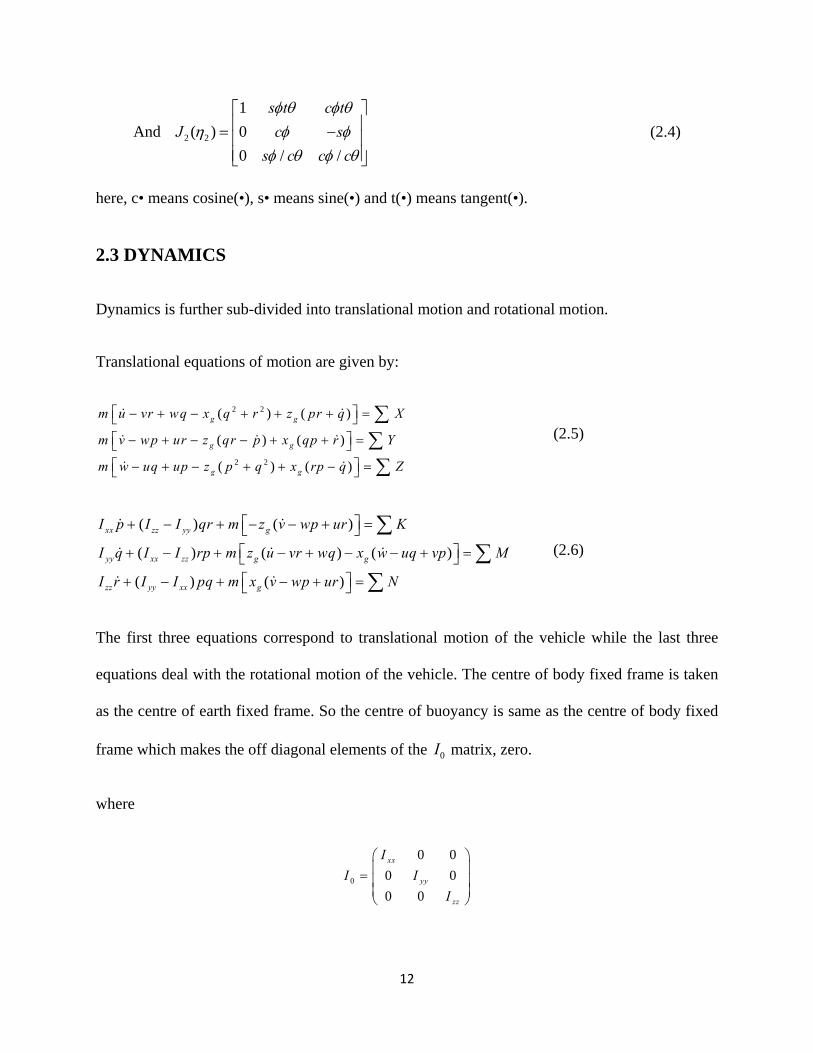
2.3 DYNAMICS

Dynamics is further sub-divided into translational motion and rotational motion.

Translational equations of motion are given by:

2 2

2 2

( ) ( )

( ) ( )

( ) ( )

g g

g g

g g

m u vr wq x q r z pr q X

m v wp ur z qr p x qp r Y

m w uq up z p q x rp q Z

(2.5)

( ) ( )

( ) ( ) ( )

( ) ( )

xx zz yy g

yy xx zz g g

zz yy xx g

I p I I qr m z v wp ur K

I q I I rp m z u vr wq x w uq vp M

I r I I pq m x v wp ur N

(2.6)

The first three equations correspond to translational motion of the vehicle while the last three

equations deal with the rotational motion of the vehicle. The centre of body fixed frame is taken

as the centre of earth fixed frame. So the centre of buoyancy is same as the centre of body fixed

frame which makes the off diagonal elements of the 0I matrix, zero.

where

0

0 0

0 0

0 0

xx

yy

zz

I

I I

I

 

13  

This technique is of great help as it reduces the complexity by making 0g g gx y z

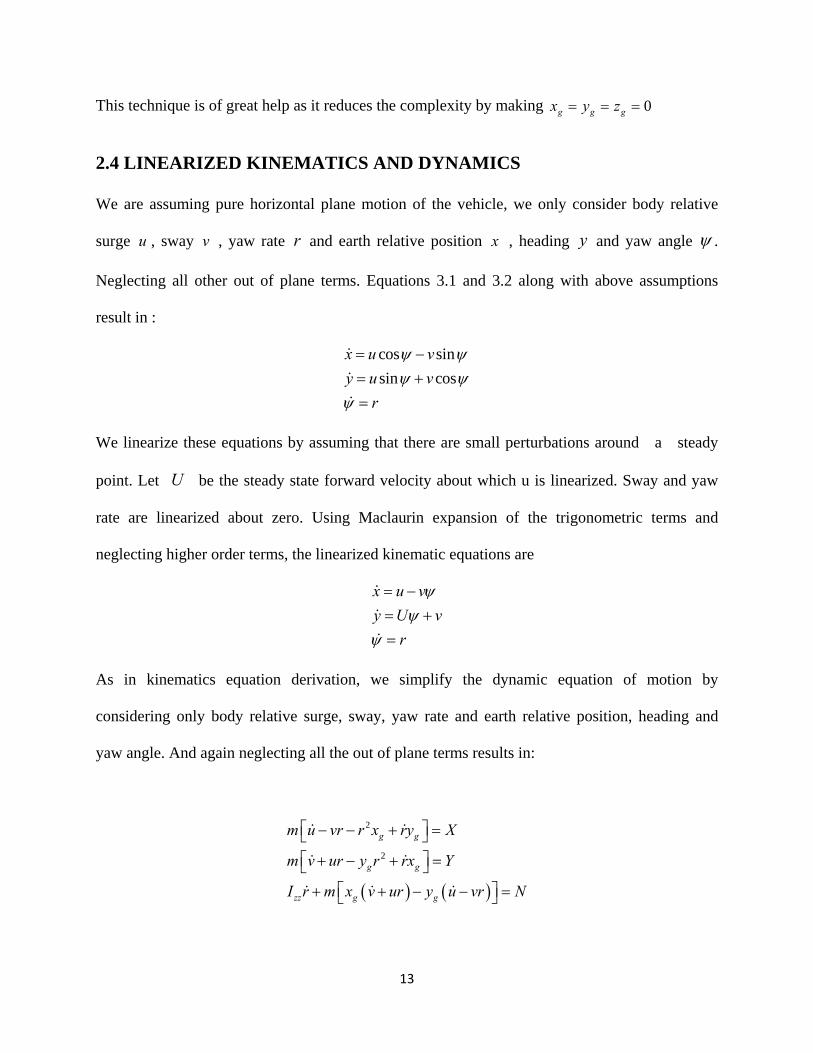
2.4 LINEARIZED KINEMATICS AND DYNAMICS

We are assuming pure horizontal plane motion of the vehicle, we only consider body relative

surge u , sway v , yaw rate r and earth relative position x , heading y and yaw angle .

Neglecting all other out of plane terms. Equations 3.1 and 3.2 along with above assumptions

result in :

cos sin

sin cos

x u v

y u v

r

We linearize these equations by assuming that there are small perturbations around a steady

point. Let U be the steady state forward velocity about which u is linearized. Sway and yaw

rate are linearized about zero. Using Maclaurin expansion of the trigonometric terms and

neglecting higher order terms, the linearized kinematic equations are

x u v

y U v

r

As in kinematics equation derivation, we simplify the dynamic equation of motion by

considering only body relative surge, sway, yaw rate and earth relative position, heading and

yaw angle. And again neglecting all the out of plane terms results in:

2

2

g g

g g

zz g g

m u vr r x ry X

m v ur y r rx Y

I r m x v ur y u vr N

 

14  

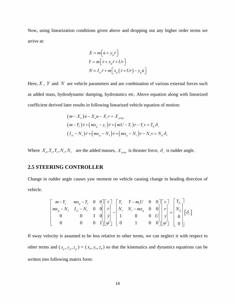
Now, using linearization conditions given above and dropping out any higher order terms we

arrive at:

g

g

zz g g

X m u y r

Y m v x r Ur

N I r m x v Ur y u

Here, X , Y and N are vehicle parameters and are combination of various external forces such

as added mass, hydrodynamic damping, hydrostatics etc. Above equation along with linearized

coefficient derived later results in following linearized vehicle equation of motion:

r

r

u u r prop

v g r r v r

zz r g v g r v r

m X u X u X r X

m Y v mx y r mU Y r Y v Y

I N r mx N v mx N r N v N

Where , , , ,u v r v rX Y Y N N are the added masses, propX is thruster force, r is rudder angle.

2.5 STEERING CONTROLLER

Change in rudder angle causes yaw moment on vehicle causing change in heading direction of

vehicle.

0 0 0 0

0 0 0 0

0 0 1 0 1 0 0 00 0 0 1 0 1 0 0 0

r

r

v g r v r

g v zz r v r gr

Ym Y mx Y v Y Y m U v

mx N I N r N N mx r N

y U y

If sway velocity is assumed to be less relative to other terms, we can neglect it with respect to

other terms and ( , ,g g gx y z ) = ( , ,b b bx y z ) so that the kinematics and dynamics equations can be

written into following matrix form:

 

15  

0 0 0 0

0 1 0 0 0 0

0 0 1 1 0 0 0

rzz r r

r

NI N r N r

y U y

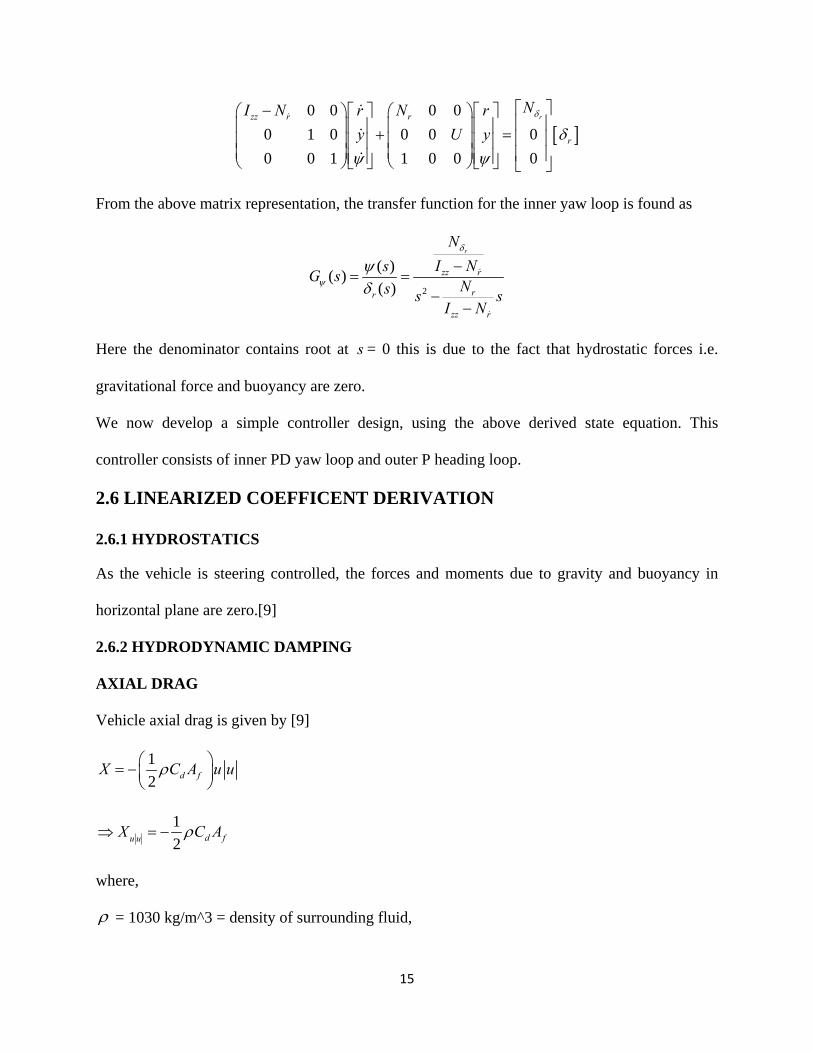
From the above matrix representation, the transfer function for the inner yaw loop is found as

2

( )( )

( )

r

zz r

rr

zz r

N

I NsG s

Ns s sI N

Here the denominator contains root at s = 0 this is due to the fact that hydrostatic forces i.e.

gravitational force and buoyancy are zero.

We now develop a simple controller design, using the above derived state equation. This

controller consists of inner PD yaw loop and outer P heading loop.

2.6 LINEARIZED COEFFICENT DERIVATION

2.6.1 HYDROSTATICS

As the vehicle is steering controlled, the forces and moments due to gravity and buoyancy in

horizontal plane are zero.[9]

2.6.2 HYDRODYNAMIC DAMPING

AXIAL DRAG

Vehicle axial drag is given by [9]

1

2 d fX C A u u

1

2 d fu uX C A

where,

= 1030 kg/m^3 = density of surrounding fluid,

 

16  

fA =0.0285 m^2= vehicle frontal area,

dC =0.3= axial drag coefficient

Linearizing,

1

2 d fX C A u U U u

2 212

2 d fC A U Uu u & 0u U U

17.6 /u d fX C A U kg s 2 /U m s

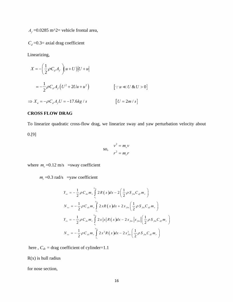
CROSS FLOW DRAG

To linearize quadratic cross-flow drag, we linearize sway and yaw perturbation velocity about

0.[9]

so, 2

2

v

r

v m v

r m r

where vm =0.12 m/s =sway coefficient

rm =0.3 rad/s =yaw coefficient

2

2

2

2

3 3

1 12 2

2 2

1 12 2

2 2

1 12 2

2 2

1 12 2

2 2

b

t

b

t

b

t

b

t

x

vc dc v fin df v

x

x

vc dc v fin fin df v

x

x

rc dc r fin fin fin df r

x

x

rc dc r fin fin df r

x

Y C m R x dx S C m

N C m xR x dx x S C m

Y C m x x R x dx x x S C m

N C m x R x dx x S C m

here , Cdc = drag coefficient of cylinder=1.1

R(x) is hull radius

for nose section,

 

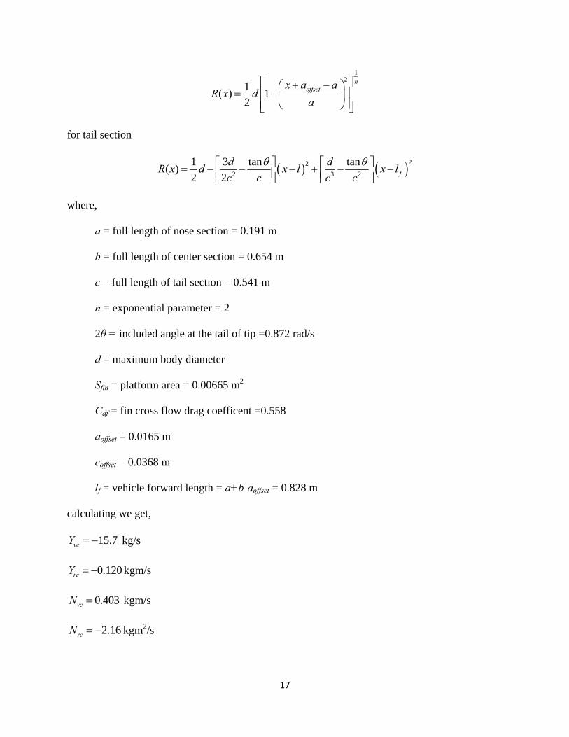
17  

12

1( ) 1

2

noffsetx a a

R x da

for tail section

22

2 3 2

1 3 tan tan( )

2 2 f

d dR x d x l x l

c c c c

where,

a = full length of nose section = 0.191 m

b = full length of center section = 0.654 m

c = full length of tail section = 0.541 m

n = exponential parameter = 2

2θ = included angle at the tail of tip =0.872 rad/s

d = maximum body diameter

Sfin = platform area = 0.00665 m2

Cdf = fin cross flow drag coefficent =0.558

aoffset = 0.0165 m

coffset = 0.0368 m

lf = vehicle forward length = a+b-aoffset = 0.828 m

calculating we get,

15.7vcY kg/s

0.120rcY kgm/s

0.403vcN kgm/s

2.16rcN kgm2/s

 

18  

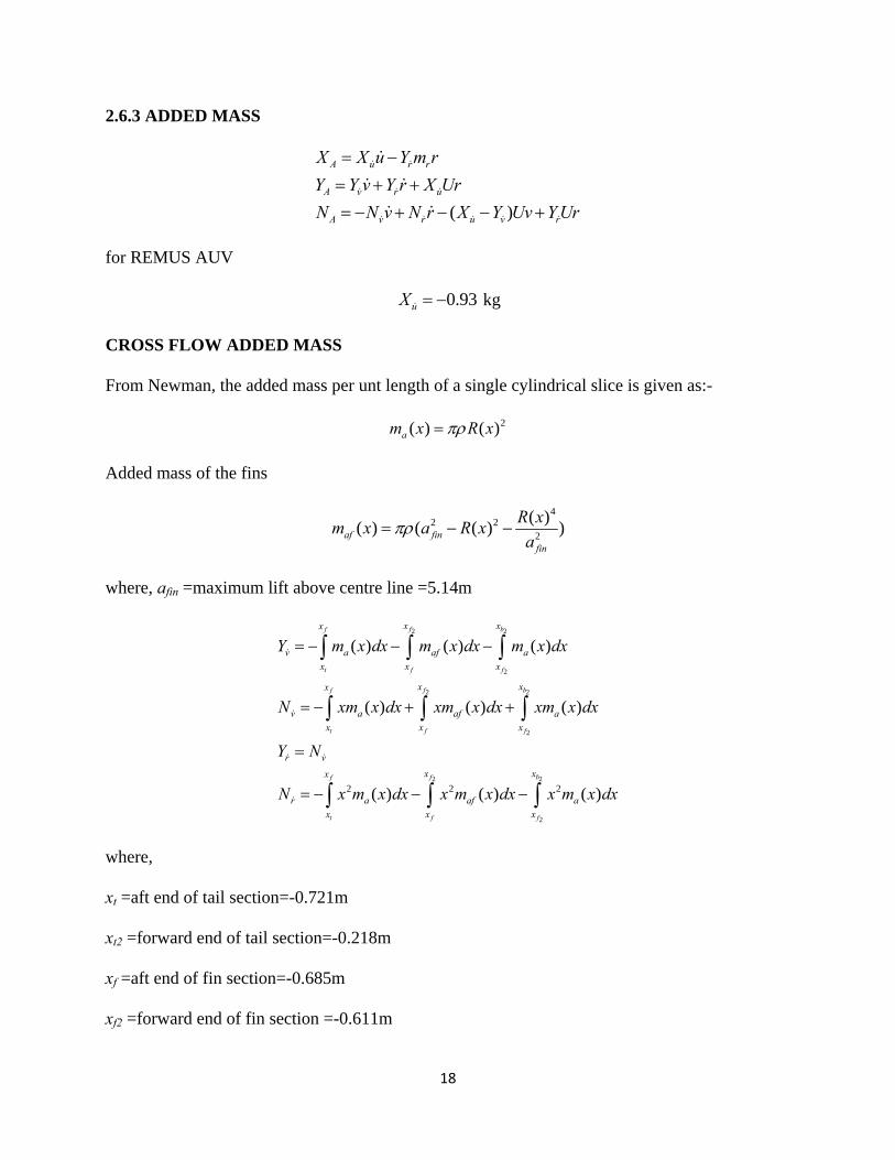
2.6.3 ADDED MASS

( )

A u r r

A v r u

A v r u v r

X X u Y m r

Y Y v Y r X Ur

N N v N r X Y Uv Y Ur

for REMUS AUV

0.93uX kg

CROSS FLOW ADDED MASS

From Newman, the added mass per unt length of a single cylindrical slice is given as:-

2( ) ( )am x R x

Added mass of the fins

42 2

2

( )( ) ( ( ) )af fin

fin

R xm x a R x

a

where, afin =maximum lift above centre line =5.14m

2 2

2

2 2

2

2 2

2

2 2 2

( ) ( ) ( )

( ) ( ) ( )

( ) ( ) ( )

f bf

t f f

f bf

t f f

f bf

t f f

x xx

v a af a

x x x

x xx

v a af a

x x x

r v

x xx

r a af a

x x x

Y m x dx m x dx m x dx

N xm x dx xm x dx xm x dx

Y N

N x m x dx x m x dx x m x dx

where,

xt =aft end of tail section=-0.721m

xt2 =forward end of tail section=-0.218m

xf =aft end of fin section=-0.685m

xf2 =forward end of fin section =-0.611m

 

19  

xb =aft end of bow section=0.437m

xb2 =forward end of bow section=0.610m

Calculating

vY=-35.5 kg

vN =1.93 kgm

rY=1.93 kgm

rN =-4.88kg 2m

The cross term results from added mass coupling

0.597

1.86

( ) 69.14

3.86

ra r r

ra u

va u v

ra r

X m Y

Y X U

N X Y U

N Y U

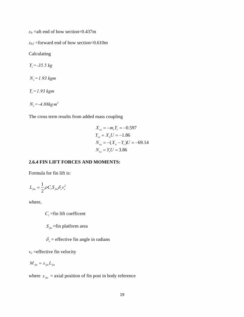
2.6.4 FIN LIFT FORCES AND MOMENTS:

Formula for fin lift is:

21

2fin l fin e eL C S v

where,

lC =fin lift coefficent

finS =fin platform area

e = effective fin angle in radians

ve =effective fin velocity

fin fin finM x L

where finx = axial position of fin post in body reference

 

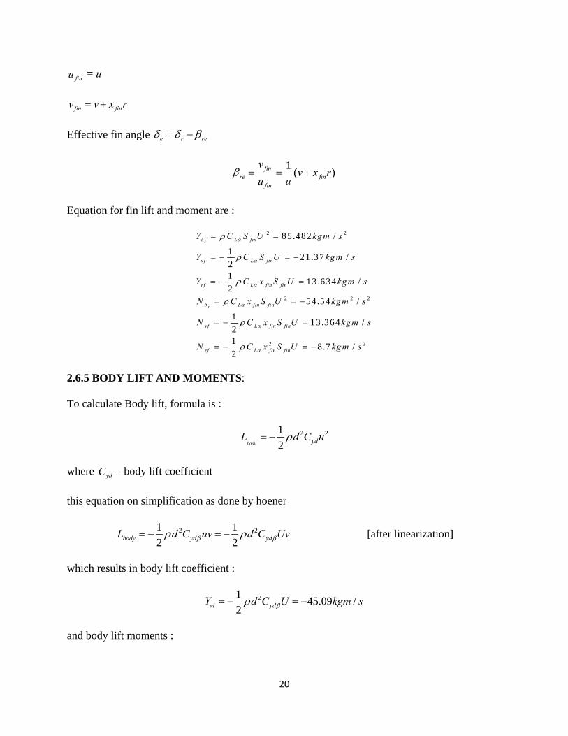
20  

finu = u

fin finv v x r

Effective fin angle e r re

1( )fin

re finfin

vv x r

u u

Equation for fin lift and moment are :

2 2

2 2 2

2 2

85 .482 /

121 .37 /

21

13.634 /2

54 .54 /

113 .364 /

21

8 .7 /2

r

r

L fin

vf L fin

rf L fin fin

L fin fin

vf L fin fin

rf L fin fin

Y C S U kgm s

Y C S U kgm s

Y C x S U kgm s

N C x S U kgm s

N C x S U kgm s

N C x S U kgm s

2.6.5 BODY LIFT AND MOMENTS:

To calculate Body lift, formula is :

2 21

2body ydL d C u

where ydC = body lift coefficient

this equation on simplification as done by hoener

2 21 1

2 2body yd ydL d C uv d C Uv [after linearization]

which results in body lift coefficient :

2145.09 /

2vl ydY d C U kgm s

and body lift moments :

 

21  

2114.474 /

2vl yd cpN d C Ux kgm s

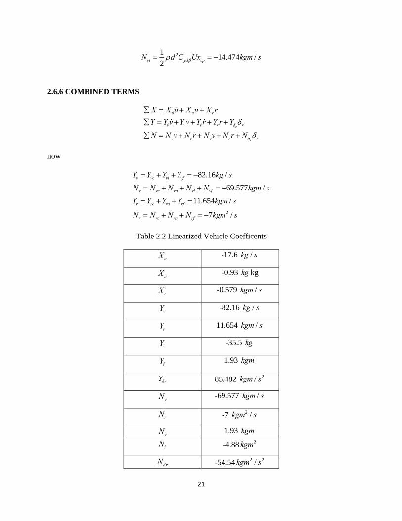
2.6.6 COMBINED TERMS

r

r

u u r

v v r r r

v r v r r

X X u X u X r

Y Y v Y v Y r Y r Y

N N v N r N v N r N

now

2

82.16 /

69.577 /

11.654 /

7 /

v vc vl vf

v vc va vl vf

r rc ra rf

r rc ra rf

Y Y Y Y kg s

N N N N N kgm s

Y Y Y Y kgm s

N N N N kgm s

Table 2.2 Linearized Vehicle Coefficents

uX -17.6 /kg s

uX -0.93 kg kg

rX -0.579 /kgm s

vY -82.16 /kg s

rY 11.654 /kgm s

vY -35.5 kg

rY 1.93 kgm

rY 85.482 2/kgm s

vN -69.577 /kgm s

rN -7 2 /kgm s

vN 1.93 kgm

rN -4.88 2kgm

rN -54.54 2 2/kgm s

 

22  

So,

2

54.543.45 4.88( )

( 7)3.45 4.88

G ss s

=2

6.547

0.84s s

Yaw control is done by PD controller with general transfer function given by

( )(1 )

( )r

p d

sK s

e s

where, e (error in yaw) = des (desired yaw) – (actual yaw). Kp is the proportional gain, d is

the derivative time constant.

Outer heading loop transfer function relates the des to y. As inner yaw loop is very fast

compared to outer heading loop, we can assume that des is nearly equal to ψ so that the transfer

function

( )

( )y

y s UG s

s s

For heading control, a proportional controller (P controller) is used whose gain,

( )

( )y

sG

e s

where ye is the error in position of the vehicle.

Adjusting in MATLAB, the controller gains are found out to be pK =-10 and dK =-2.5

 

23  

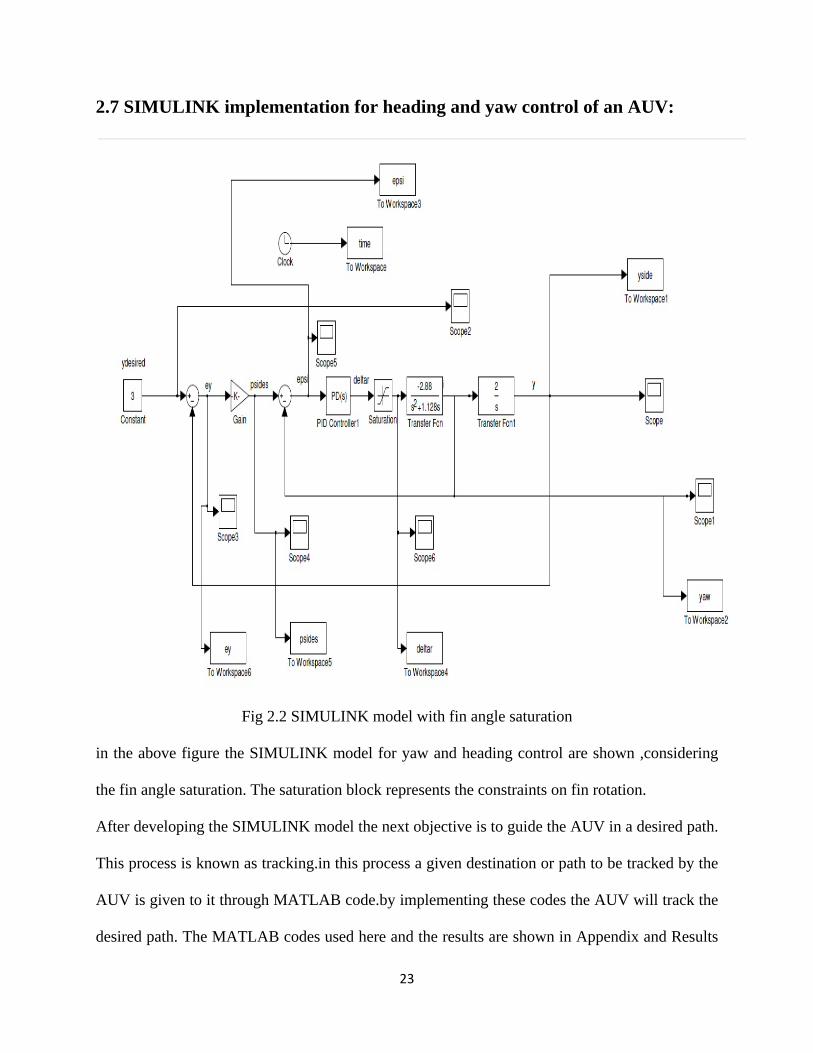
2.7 SIMULINK implementation for heading and yaw control of an AUV:

Fig 2.2 SIMULINK model with fin angle saturation

in the above figure the SIMULINK model for yaw and heading control are shown ,considering

the fin angle saturation. The saturation block represents the constraints on fin rotation.

After developing the SIMULINK model the next objective is to guide the AUV in a desired path.

This process is known as tracking.in this process a given destination or path to be tracked by the

AUV is given to it through MATLAB code.by implementing these codes the AUV will track the

desired path. The MATLAB codes used here and the results are shown in Appendix and Results

 

24  

section respectively. We have derived a linear model of AUV in x-y plane. While trying to

implement AUV dynamics in MATLAB we use a non-linear model as the controller will try to

operate at the desired velocity and will linearize it about that point. So the controller will be

effective on non-linear plant model.

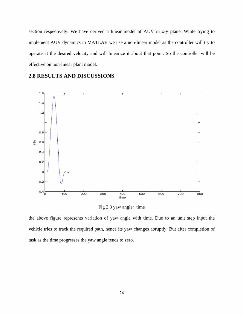
2.8 RESULTS AND DISCUSSIONS

Fig 2.3 yaw angle~ time

the above figure represents variation of yaw angle with time. Due to an unit step input the

vehicle tries to track the required path, hence its yaw changes abruptly. But after completion of

task as the time progresses the yaw angle tends to zero.

 

25  

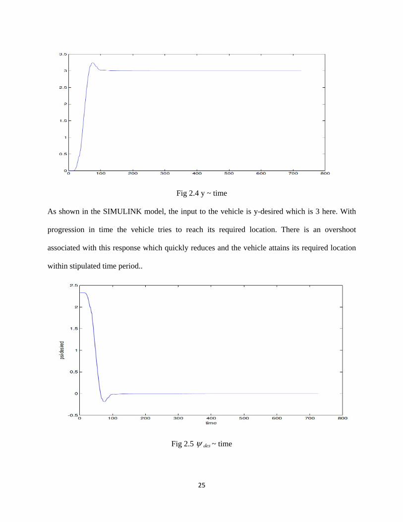
Fig 2.4 y ~ time

As shown in the SIMULINK model, the input to the vehicle is y-desired which is 3 here. With

progression in time the vehicle tries to reach its required location. There is an overshoot

associated with this response which quickly reduces and the vehicle attains its required location

within stipulated time period..

Fig 2.5 des ~ time

 

26  

Due to the step input, the value of des changes accordingly. At the beginning a sudden change

in the value of des is observed. As time progresses the vehicle achieves its required des value,

hence des decreases and reaches zero value.

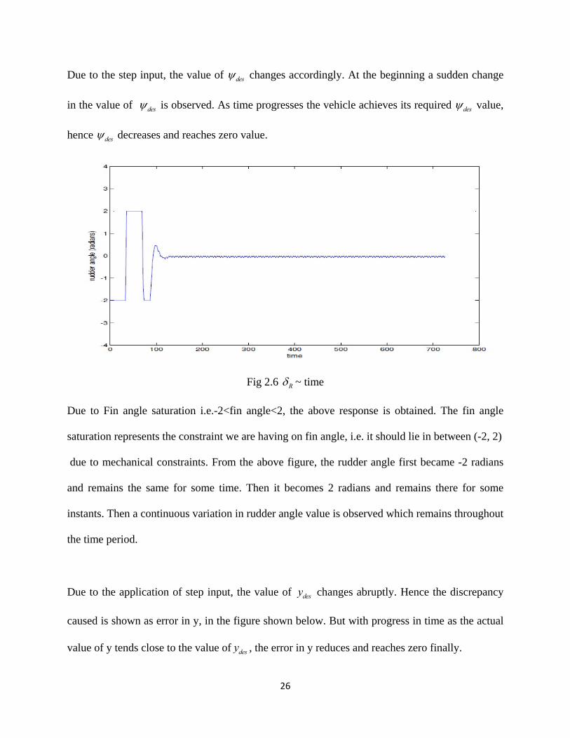
Fig 2.6 R ~ time

Due to Fin angle saturation i.e.-2<fin angle<2, the above response is obtained. The fin angle

saturation represents the constraint we are having on fin angle, i.e. it should lie in between (-2, 2)

due to mechanical constraints. From the above figure, the rudder angle first became -2 radians

and remains the same for some time. Then it becomes 2 radians and remains there for some

instants. Then a continuous variation in rudder angle value is observed which remains throughout

the time period.

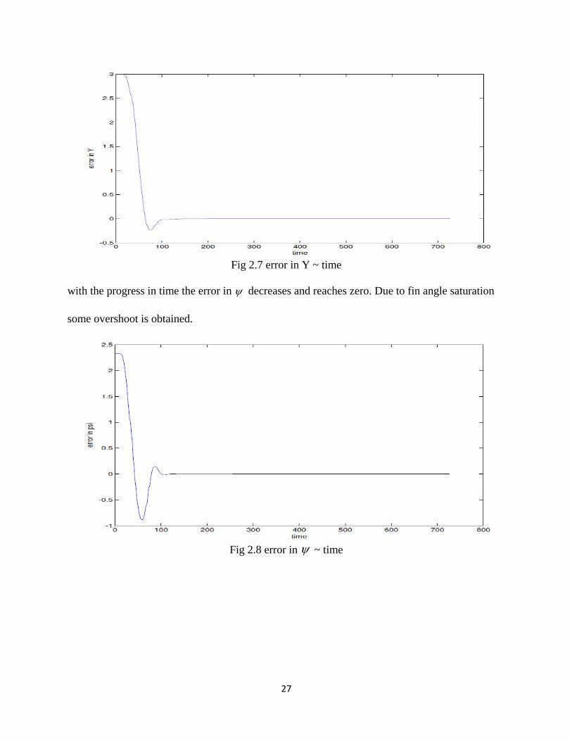
Due to the application of step input, the value of desy changes abruptly. Hence the discrepancy

caused is shown as error in y, in the figure shown below. But with progress in time as the actual

value of y tends close to the value of desy , the error in y reduces and reaches zero finally.

 

27  

Fig 2.7 error in Y ~ time

with the progress in time the error in decreases and reaches zero. Due to fin angle saturation

some overshoot is obtained.

Fig 2.8 error in ~ time

 

28  

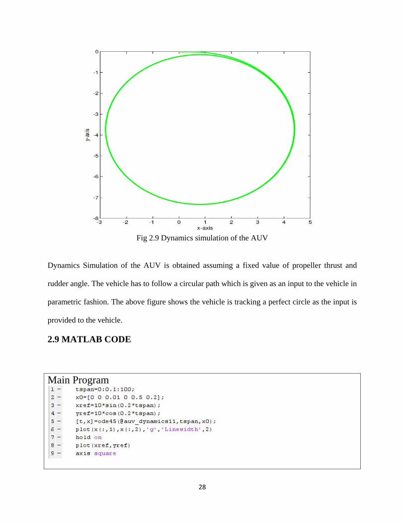
Fig 2.9 Dynamics simulation of the AUV

Dynamics Simulation of the AUV is obtained assuming a fixed value of propeller thrust and

rudder angle. The vehicle has to follow a circular path which is given as an input to the vehicle in

parametric fashion. The above figure shows the vehicle is tracking a perfect circle as the input is

provided to the vehicle.

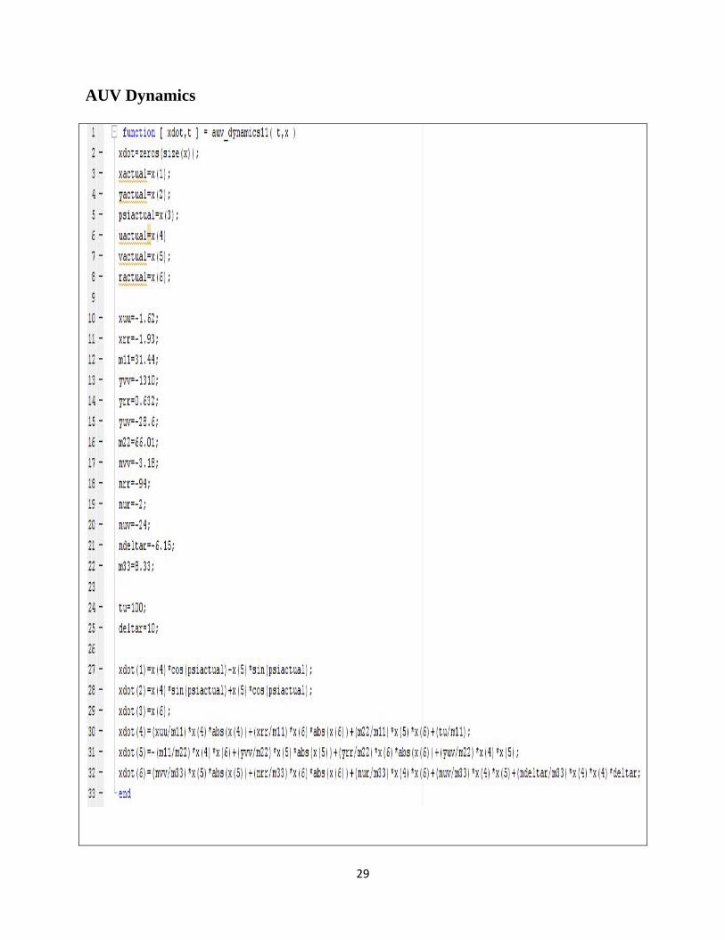
2.9 MATLAB CODE

Main Program

 

29  

AUV Dynamics

 

30  

2.10 Summary

A brief discussion on the kinematics and dynamics of the underwater vehicle is given in this

chapter. The nonlinear dynamics equations of the vehicle are formulated and linearized. The

linear coefficients of the vehicle are calculated and used to form the transfer function model of

the vehicle. The SIMULINK model is used to study the heading control of the vehicle along with

the MATLAB simulation for vehicle dynamics.

 

31  

CHAPTER 3

HEADING CONTROL OF UNDERWATER VEHICLE

A six degree-of-freedom rigid body motion in space is typically considered for determining ship

response in waves. For ship maneuvering study a three degree-of-freedom plane motion is

usually considered sufficient. However, for high speed vessels like the container ships, turning

motion induced roll is very high so cannot be neglected. Hence a four degree-of-freedom

description that includes surge, sway, yaw and roll modes is needed. Since the hydrodynamics

involved in ship steering is highly nonlinear, coupled nonlinear differential equations are needed

to fully describe the complicated ship maneuvering dynamics. A simple transfer function model

description is usually preferred when a qualitative prediction capability is all we need from the

model. This is the case in a model-based controller design, since the feedback controller itself

tolerates certain amount of modeling error and a complicated model might result in a controller

too complicated to implement. The popularity of the first order Nomoto model in ship steering

autopilot design is due to its simplicity and relative accuracy in describing the course-keeping

yaw dynamics, where typically, small rudder angles are involved. Extension to large rudder

angle yaw dynamics basing upon the Nomoto model has been proposed to better describe the

nonlinear behavior of yaw dynamics.

3.1 NOMOTO MODEL

NOMOTO model is a linear ship steering model which uses first order or second order models

for ship steering autopilot design. The advantage of this model over others is its simplicity and

accuracy in tracking yaw dynamics.

Linear theory suggests we can write equations of motion as :

 

32  

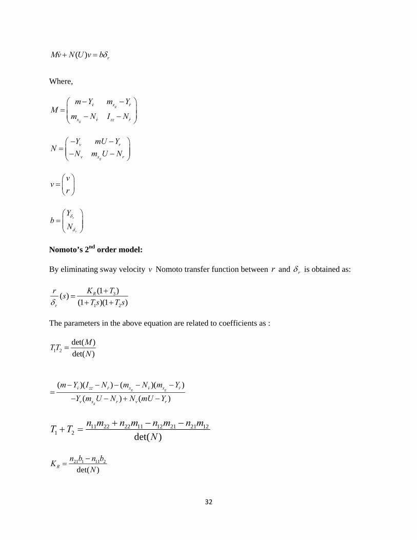
( ) rMv N U v b

Where,

g

g

v x r

x v zz r

m Y m YM

m N I N

g

v r

v x r

Y mU YN

N m U N

vv

r

r

r

Yb

N

Nomoto’s 2nd order model:

By eliminating sway velocity v Nomoto transfer function between r and r is obtained as:

3

1 2

(1 )( )

(1 )(1 )R

r

K Trs

T s T s

The parameters in the above equation are related to coefficients as :

1 2

det( )

det( )

MTT

N

( )( ) ( )( )

( ) ( )g g

g

v zz r x v x r

v x r v r

m Y I N m N m Y

Y m U N N mU Y

11 22 22 11 12 21 21 121 2 det( )

n m n m n m n mT T

N

21 1 11 2

det( )R

n b n bK

N

 

33  

21 1 11 23 det( )R

m b m bK T

N

1 2

( ) ( )( ) ( )( ) ( )

det( )g g gv zz r x r v r x v v x rY I N m U N m Y mU Y m N N m Y

T TN

det( )r rv v

R

N Y Y NK

N

3

( ) ( )

det( )g r rx v v

R

m N Y m Y NK T

N

3 32

1 2 1 2 1 2

(1 )( )

( ) (1 )(1 ) ( ) 1R R R

r

K T s K K T sr s

s T s T s TT s T T s

3 1.9103RK T

det( ) ( )( ) ( )( )g gv zz r x v x rM m Y I N m N m Y

=546.1384

det( ) ( ) ( )gv x r v rN Y m U N N mU Y

= -1798.221

1 2

det( )0.3037

det( )

MT T

N

1 2 0.74884T T 5.799RK

2

( ) 1.9103 5.799

( ) 0.3037 0.7488 1r

r s s

s s s

Nomoto’s 1st order model :

In this model approximation is found out by using a effective time constant

1 2 3T T T T

 

34  

This first order model works well only for low frequency operation as it gives good results but as

the frequency is increased the approximation starts giving erronious results hence second order

model is preferred in such cases.

1 2 3

( )(1 )

1.0782

KH s

s Ts

where

T T T T

2

5.799

1.0782s s

3.2 NOMOTO MODEL ANALYSIS USING SIMULINK

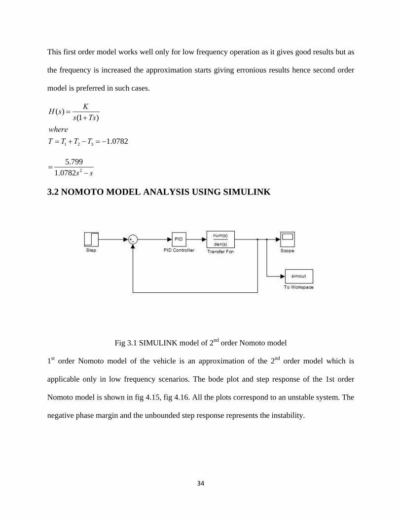
Fig 3.1 SIMULINK model of 2nd order Nomoto model

1st order Nomoto model of the vehicle is an approximation of the 2nd order model which is

applicable only in low frequency scenarios. The bode plot and step response of the 1st order

Nomoto model is shown in fig 4.15, fig 4.16. All the plots correspond to an unstable system. The

negative phase margin and the unbounded step response represents the instability.

 

35  

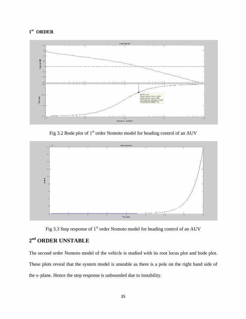
1st ORDER

Fig 3.2 Bode plot of 1st order Nomoto model for heading control of an AUV

Fig 3.3 Step response of 1st order Nomoto model for heading control of an AUV

2nd ORDER UNSTABLE

The second order Nomoto model of the vehicle is studied with its root locus plot and bode plot.

These plots reveal that the system model is unstable as there is a pole on the right hand side of

the s–plane. Hence the step response is unbounded due to instability.

 

 

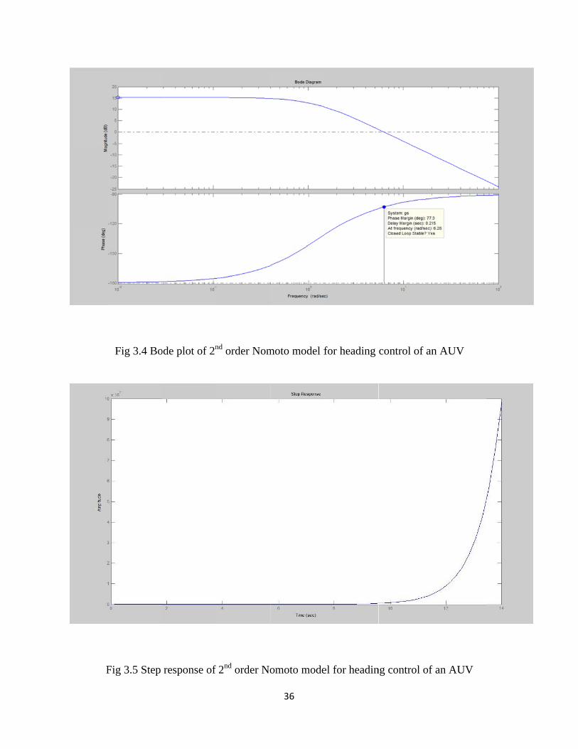
F

Fig 3.4 Bo

Fig 3.5 Step

ode plot of 2n

response of

nd order Nom

f 2nd order No

36 

moto model f

omoto mode

for heading

el for headin

control of an

ng control of

n AUV

f an AUV

 

37  

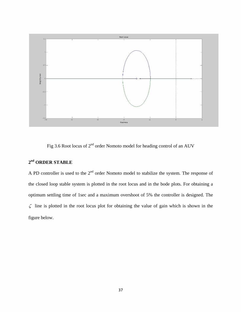
Fig 3.6 Root locus of 2nd order Nomoto model for heading control of an AUV

2nd ORDER STABLE

A PD controller is used to the 2nd order Nomoto model to stabilize the system. The response of

the closed loop stable system is plotted in the root locus and in the bode plots. For obtaining a

optimum settling time of 1sec and a maximum overshoot of 5% the controller is designed. The

line is plotted in the root locus plot for obtaining the value of gain which is shown in the

figure below.

 

38  

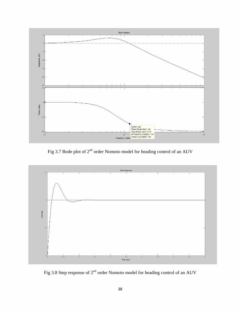
Fig 3.7 Bode plot of 2nd order Nomoto model for heading control of an AUV

Fig 3.8 Step response of 2nd order Nomoto model for heading control of an AUV

 

39  

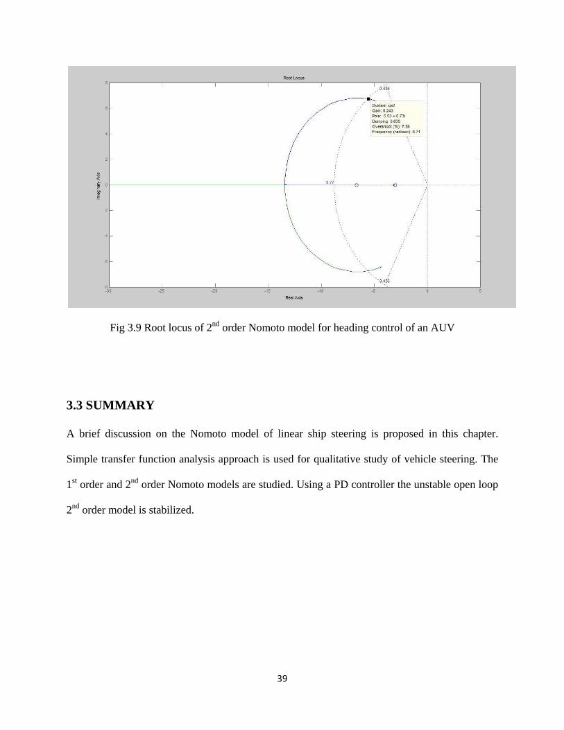
Fig 3.9 Root locus of 2nd order Nomoto model for heading control of an AUV

3.3 SUMMARY

A brief discussion on the Nomoto model of linear ship steering is proposed in this chapter.

Simple transfer function analysis approach is used for qualitative study of vehicle steering. The

1st order and 2nd order Nomoto models are studied. Using a PD controller the unstable open loop

2nd order model is stabilized.

 

40  

CHAPTER 4:

PATH TRACKING OF AN AUV

Here the objective is to drive a robot along a desired trajectory. As the name suggests an

Autonomous Underwater vehicle should be capable of task completion without using any

external input. In tracking a desired path is to be followed by the AUV. Error dynamics is

considered for tracking purpose here. The error associated with heading and surge is calculated

and constantly minimized for required system performance.

An AUV can be designed in various different ways. Each of these designs have their own

advantages and disadvantages. For example such designs can be categorized as

I. Torpedo shape

II. One hull, four thrusters

III. Two hulls, four thrusters

IV. Two hulls, two rotating thrusters

Here the trajectory tracking for a torpedo shaped and a two hulls, two rotating thrusters type

AUV is studied.

TORPEDO SHAPED AUV

4.1 ERROR DYNAMICS

We first derive error dynamics of the vehicle from its dynamics.

e du u u

e rr r

Where ,u r are actual surge and heading rate

,d ru are desired surge and heading rate

 

41  

Assuming constant desired surge velocity du = 2 m/s

eu u and

( ) ( ) ( )propu r

eu u u

XX Xu u r

m X m X m X

So the forward speed control law is

31.44( )prop u u uX f k e

And similarly yaw dynamics is defined as

2.952rr f r

So steering control law is

0.33875( )r rr f K r

Using these control laws propeller thrust force and rudder angle control the dynamics of the

vehicle and a circular path is followed by the vehicle.

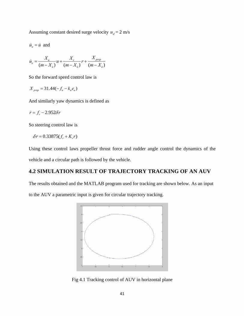
4.2 SIMULATION RESULT OF TRAJECTORY TRACKING OF AN AUV

The results obtained and the MATLAB program used for tracking are shown below. As an input

to the AUV a parametric input is given for circular trajectory tracking.

Fig 4.1 Tracking control of AUV in horizontal plane

 

42  

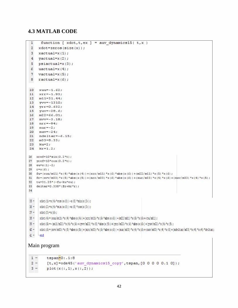
4.3 MATLAB CODE

Main program

 

43  

TWO THRUSTERS MODEL

The trajectory tracking of two thrusters model is comparatively simpler than the torpedo shaped

model. The controller required for trajectory tracking is proposed in two different methods i.e.

using PD controller and LQR based control.

The simulation result and the MATLAB program used for achieving trajectory tracking is shown

below.

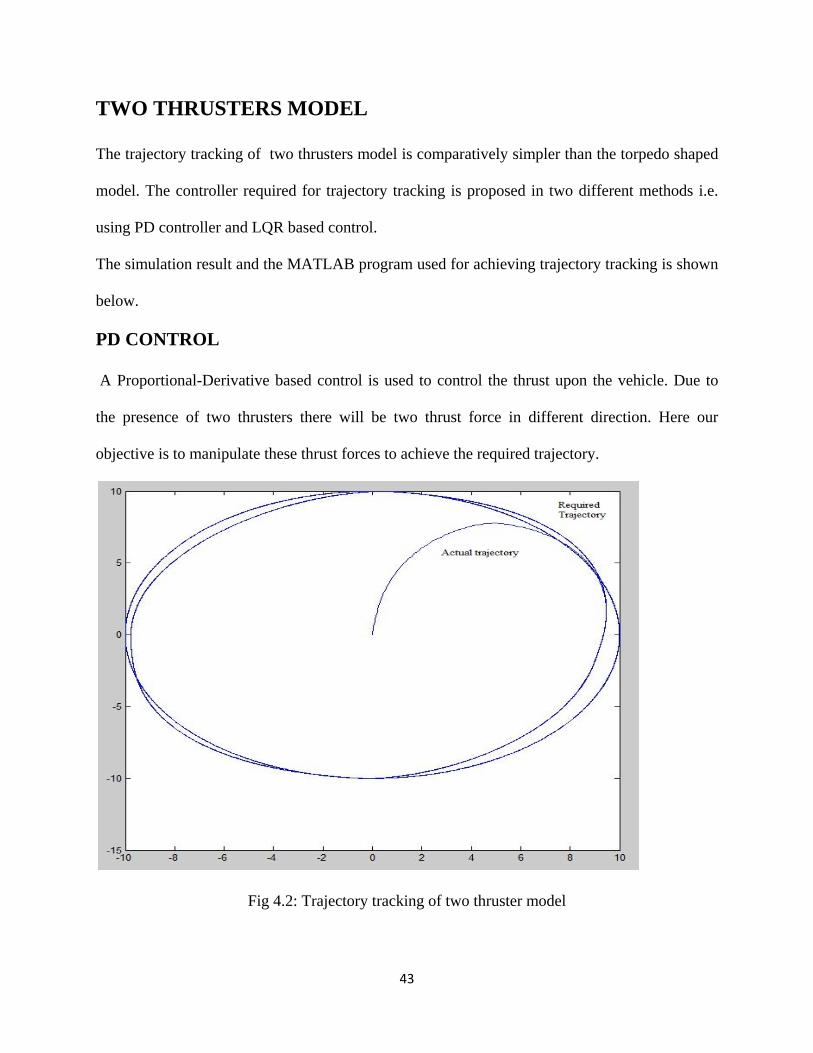
PD CONTROL

A Proportional-Derivative based control is used to control the thrust upon the vehicle. Due to

the presence of two thrusters there will be two thrust force in different direction. Here our

objective is to manipulate these thrust forces to achieve the required trajectory.

Fig 4.2: Trajectory tracking of two thruster model

 

44  

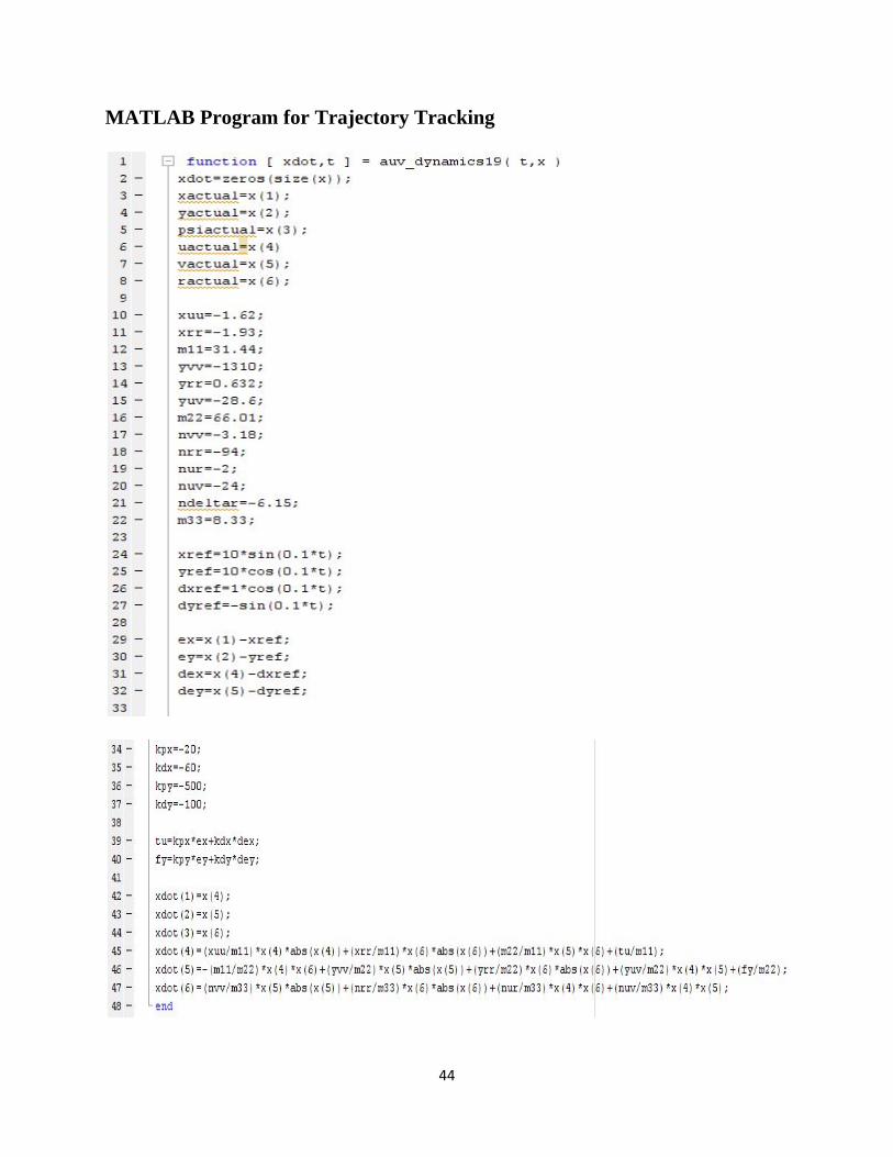
MATLAB Program for Trajectory Tracking

 

45  

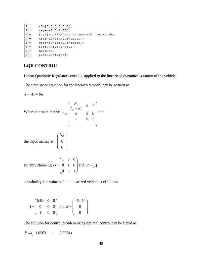
LQR CONTROL

Linear Quadratic Regulator control is applied to the linearised dynamics equation of the vehicle.

The state space equation for the linearized model can be written as :

x Ax Bu

Where the state matrix

0 0

0 0

1 0 0

r

zz r

N

I N

A U

and

the input matrix 0

0

rN

B

suitably choosing

1 0 0

0 1 0

0 0 1

Q

and 1R

substituting the values of the linearized vehicle coefficients

0.84 0 0

0 0 2

1 0 0

A

and

54.54

0

0

B

The solution for control problem using optimal control can be stated as

1.0563 1 2.2724K

 

46  

CHAPTER 5:

CONCLUSIONS AND SUGGESTIONS FOR FUTURE WORK

In this thesis modeling of AUV is done and kinematics and dynamic equations of motion were

obtained. Using geometrical parameters and relevant empirical formulas various hydrodynamic

coefficients for the dynamic model are determined. Various methods for heading control of AUV

were developed and controllers were designed.

Transfer function for heading control of AUV using simple P-PD controller was designed and

simulation results were obtained to see the accuracy of the model obtained. Also, a Nomoto

model approximation was presented and both 1st order and 2nd order models were obtained.

Control of Nomoto model using PD controller is done with some design parameters pre-

assigned. The stability of model obtained is visible in results obtained.

Path following problem of AUV in horizontal plane is considered and using error dynamics

reduction technique on the surge velocity u and heading rate r , it was implemented. The

required path is given in parametric form to the AUV.

Depth control and obstacle avoidance are major requirements for an AUV. Then for more

complex operations a leader follower model has to be implemented. Their formation control is a

major research field now-a-days.

 

47  

REFERENCES:

[1] Breivik, Morten and Fossen. Thor I. “Guidance Laws for Autonomous Underwater

Vehicles”. Norwegian University of Science and Technology, Norway.

[2] Blidberg, D Richard. “The Development of Autonomous Underwater Vehicles (AUV);

A Brief Summary”. Autonomous Undersea Systems Institute, Lee New Hampshire, USA.

[3] Desa, Elgar. , Madhan, R. and Maurya, P. “Potential of autonomous underwater vehicles

as new generation ocean data platforms”. National Institute of Oceanography, Dona

Paula, Goa, India.

[4] Ching-Yaw Tzeng, Ju-Fen Chen.” Fundamental properties of linear ship steering

dynamic models ”, Journal of Marine Science and Technology, Vol. 7, No. 2(1999): pp.

79-88

[5] http://robotics.ee.uwa.edu.au/auv/usal.html

[6] O. Xu. Autonomous underwater vehicles (auvs). Report, The University of Western

Australia, 2004.

[7] http://ise.bc.ca/design_sensors.html

[8] Fossen, Thor I. “Guidance and Control of Ocean Vehicles”. Wiley, New York, 1994

[9] Prestero, Timothy. “Verification of a Six-Degree of Freedom Simulation Model of

REMUS

[10] Autonomous Underwater Vehicle”. MIT and WHOI. 2001.