The Study of External Conditions on Lake Erie

Laura Carpenter

REU SUR-WinD project Case Western Reserve University

Mentor: Dr. Matthiesen Graduate Student Assistant: Daniel Corrigan

PIs: Dr. I. Alexander and Dr. J. R. Kadambi July 26, 2013

Carpenter 2

Table of Contents

1. Abstract 3

2. Introduction 3

3. Methodology 4

a. Instrument Deployment and Data Retrieval 4

b. Upward Looking Sonar 5

c. SWIP Theory of Operation 6

d. Ice Draft 7

e. Processing Data 8

f. IPS Processing Toolbox 8

g. 50 Year Return Wave Assessment 9

4. Results and Discussion 9

a. Ice and Wave Data Analysis 9

b. WERC Website 13

c. 50 Year Return Wave 13

5. Summary of Conclusions 15

6. Acknowledgements 15

7. References 15

Carpenter 3

Abstract

As the offshore wind turbine farm project, Icebreaker, is in developing stages a growing

understanding of the external conditions on Lake Erie is vital. Ice thickness and wave amplitude are

both concerns. The SWIP (Shallow Water Ice Profiler) collected ice and wave data in Lake Erie from

December 2010 through April 2013. The data shows 6 meter thick ice on January 17, 2011. This most

likely was an ice sheet forced vertical by ridging. When excluding occurrences like these a maximum ice

sheet thickness of slightly over 1 meter is present. The SWIP data reveals waves reaching 1.5 meters in

amplitude. Severe storms cause the readings to be exaggerated which could easily have been the case

here. Typically the wave amplitudes were .5 meters or below.

LEEDCo, The leader of the Icebreaker project hired several companies with expertise in risk

analysis to do a feasibility study on the external conditions of Lake Erie. One wave assessment

specification required calculating the 50 year return wave. Case Western Reserve University is

responsible for confirming the results of this study. By plotting the annual maximum wave heights from

NOAA buoyee 45005 against the annual probability of occurrence and applying a Weibel distribution it

was determined that the 50 year return wave height is 3.75 meters.

Introduction

Case Western Reserve University has an important role to play in LEEDCo’s effort to install an

offshore wind turbine farm in Lake Erie. As a research university Case has the capacity to perform

research on the external conditions of the lake including the ice, wind, and wave conditions. With this

research Case is developing and spreading an understanding of the feasibility of the Icebreaker project.

The vision of this project is to install six 3MW wind turbines 7.5 miles off of Cleveland in Lake Erie. The

larger picture is to spark a wind energy movement throughout the Great Lakes Region. With this vision

at hand my specific project this summer was to study the ice and waves on Lake Erie.

Carpenter 4

In December 2010 an active sonar device was placed in Lake Erie to study ice. My objective for

the summer was to analyze all three years of the collected data. This operation was to be performed in

Matlab using the IPS5 Processing Toolbox. The goal was to be able to speak of an average ice thickness

and an average wave amplitude for Lake Erie. As the summer progressed I was also given the task of

forming a website for my research group. This website would function as a platform for organizing large

masses of data. My research team has data from the campus wind turbine, the two turbines in Euclid

which power StampCo and SOPCO, the lidar which is located on Cleveland’s water intake crib, etc. The

website was envisioned as a place to store and organize this data as well as reach out to the public in an

educational manner.

In the last couple weeks I was given a statistical analysis project. LEEDCo hired Germanischer

Lloyd, BrownFlynn, and many other companies to assess the feasibility of a wind turbine farm on Lake

Erie. The offshore wind farm standards set forth in the International Standard, IEC booklet guided this

project. The assessors determined that the wind farm is in fact feasible. Case is the ‘second opinion’ to

the on this matter, so my job was to perform the assessment for the 50 return wave and compare my

results to the feasibility report completed by these companies.

Methodology

a. Instrument Deployment and Data Retrieval

The Shallow Water Ice Profiler (SWIP) is an upward looking sonar (ULS) instrument designed to study

ice thickness. It is also useful in studying waves.

Carpenter 5

The finer parts of this instrument are capsulated inside an aluminum pressure case which is hard-coat

anodized to reduce corrosion from the water. The cylindrical piece on the top is the source of the sonar

waves emitted into the lake [1]. Professor Matthiesen and his team placed this instrument about 2-3

miles out in Lake Erie (directly off of Cleveland) at the end of 2010. It collected data for a total of three

years. The instrument settings were adjusted according to the SWIP Operators Manual. The modes of

operation include ice mode and wave mode. As would be expected the ice mode is set up with

parameters specific to detecting ice while the wave mode is programmed for detecting wave action. For

the ice mode the ping period is set to 1 Hz, and for the wave mode it is set to 2 Hz. This is simply the

rate at which the instrument sends out sonar [1]. In Cleveland waves are expected in December and ice

January through March so the ice mode is activated in December (phase 1) and the wave mode January

through April (phase 2). Inside the instrument is a flash card which stores the collected data. While in

the water the instrument can communicate with a computer by the program IPS5Link. The data may

also be transferred to a computer using the card and then extracted into a form readable by ASL’s IPS

Processing Toolbox which is accessible in Matlab [1].

b. Upward Looking Sonar

The SWIP is a modern version of Upward Looking Sonar (ULS) which has been used for over 40 years to

study ice. In the 1960’s the Artic Ice Pack was studied using sensors attached to submarines. Further, in

the 1980’s studies were performed in Canada using sensors mounted to the bottom of the body of

SWIP

Carpenter 6

water [2]. In this same time frame an invention entered the scientific community enabling ice velocity

measurements, this being acoustic Doppler current profilers. All of these endeavors have led to the Ice

Profiling Sonar (IPS) instrument which is credited to Dr. Humfrey Melling of the Canadian Department of

Fisheries and Oceans at the Institute of Ocean Sciences (IOS) [2]. In 1995 the IPS was revamped and

upgraded to the IPS4 which had more memory capacity and an increased echo sounder frequency. This

unit entered the market in 1996, followed by the IPS5 in 2007. This generation has the ability to

monitor multiple targets per ping [2]. The SWIP is simply a shallow water version of the IPS5. Since Lake

Erie’s average water depth varies between 13 meters and 17 meters in the area of deployment the SWIP

was the appropriate instrument [3].

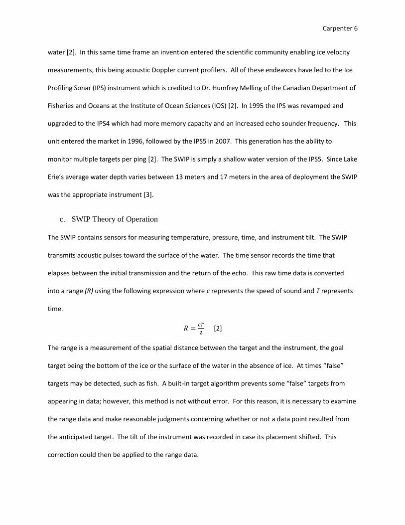
c. SWIP Theory of Operation

The SWIP contains sensors for measuring temperature, pressure, time, and instrument tilt. The SWIP

transmits acoustic pulses toward the surface of the water. The time sensor records the time that

elapses between the initial transmission and the return of the echo. This raw time data is converted

into a range (R) using the following expression where c represents the speed of sound and T represents

time.

[2]

The range is a measurement of the spatial distance between the target and the instrument, the goal

target being the bottom of the ice or the surface of the water in the absence of ice. At times “false”

targets may be detected, such as fish. A built-in target algorithm prevents some “false” targets from

appearing in data; however, this method is not without error. For this reason, it is necessary to examine

the range data and make reasonable judgments concerning whether or not a data point resulted from

the anticipated target. The tilt of the instrument was recorded in case its placement shifted. This

correction could then be applied to the range data.

Carpenter 7

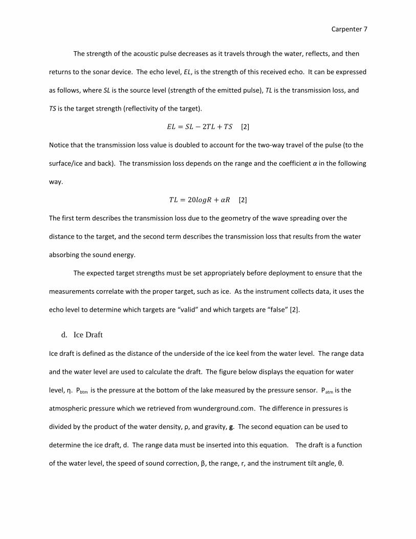
The strength of the acoustic pulse decreases as it travels through the water, reflects, and then

returns to the sonar device. The echo level, EL, is the strength of this received echo. It can be expressed

as follows, where SL is the source level (strength of the emitted pulse), TL is the transmission loss, and

TS is the target strength (reflectivity of the target).

[2]

Notice that the transmission loss value is doubled to account for the two-way travel of the pulse (to the

surface/ice and back). The transmission loss depends on the range and the coefficient α in the following

way.

[2]

The first term describes the transmission loss due to the geometry of the wave spreading over the

distance to the target, and the second term describes the transmission loss that results from the water

absorbing the sound energy.

The expected target strengths must be set appropriately before deployment to ensure that the

measurements correlate with the proper target, such as ice. As the instrument collects data, it uses the

echo level to determine which targets are “valid” and which targets are “false” [2].

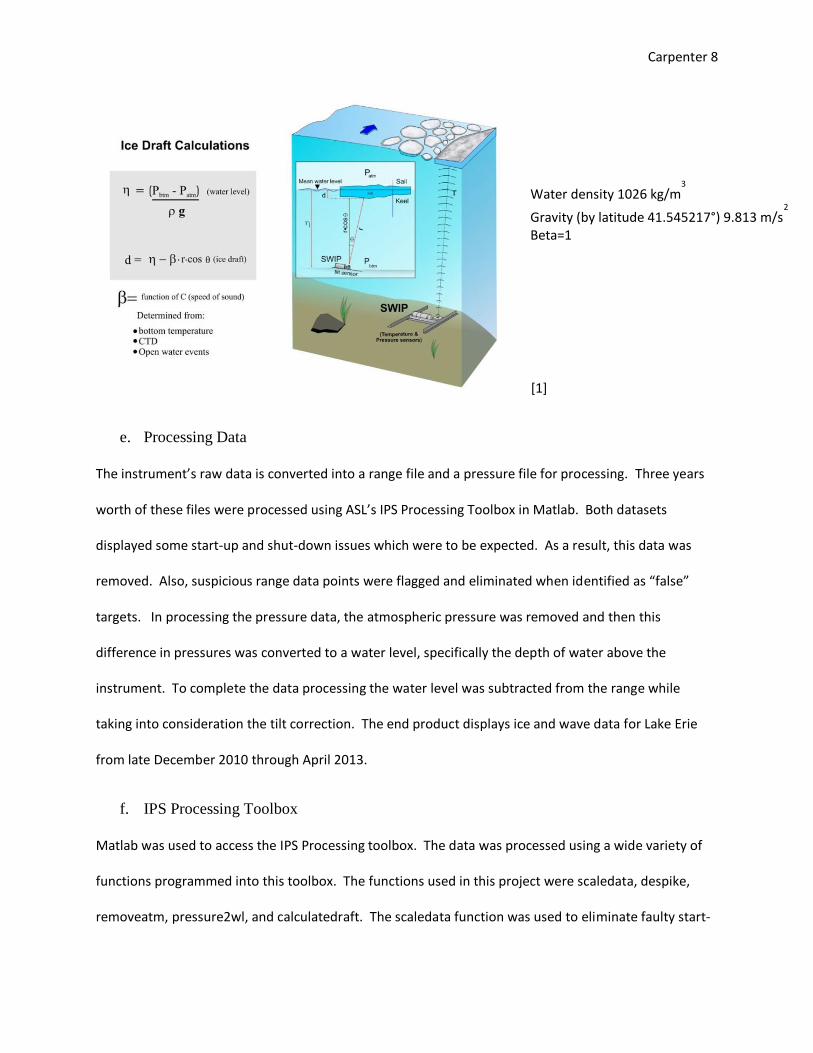
d. Ice Draft

Ice draft is defined as the distance of the underside of the ice keel from the water level. The range data

and the water level are used to calculate the draft. The figure below displays the equation for water

level, η. Pbtm is the pressure at the bottom of the lake measured by the pressure sensor. Patm is the

atmospheric pressure which we retrieved from wunderground.com. The difference in pressures is

divided by the product of the water density, ρ, and gravity, g. The second equation can be used to

determine the ice draft, d. The range data must be inserted into this equation. The draft is a function

of the water level, the speed of sound correction, β, the range, r, and the instrument tilt angle, θ.

Carpenter 8

[1]

e. Processing Data

The instrument’s raw data is converted into a range file and a pressure file for processing. Three years

worth of these files were processed using ASL’s IPS Processing Toolbox in Matlab. Both datasets

displayed some start-up and shut-down issues which were to be expected. As a result, this data was

removed. Also, suspicious range data points were flagged and eliminated when identified as “false”

targets. In processing the pressure data, the atmospheric pressure was removed and then this

difference in pressures was converted to a water level, specifically the depth of water above the

instrument. To complete the data processing the water level was subtracted from the range while

taking into consideration the tilt correction. The end product displays ice and wave data for Lake Erie

from late December 2010 through April 2013.

f. IPS Processing Toolbox

Matlab was used to access the IPS Processing toolbox. The data was processed using a wide variety of

functions programmed into this toolbox. The functions used in this project were scaledata, despike,

removeatm, pressure2wl, and calculatedraft. The scaledata function was used to eliminate faulty start-

Water density 1026 kg/m3

Gravity (by latitude 41.545217°) 9.813 m/s2

Beta=1

Carpenter 9

up/shut-down data at the beginning or end of the dataset. This function was primarily performed on

the pressure data. The despike function was used frequently on the range data. It eliminated data

points from “false” targets, such as fish or anything else in the water that reflects the sound waves.

Data points from “false” targets were recognized as points in which the range increased or decreased

dramatically within just fives seconds. In these cases it was unreasonable to believe that the range was

truly the distance between the profiler and the water surface or ice at that moment in time. The

despike function was very useful as it cleaned up the data to reflect reality more accurately. Once the

range data was fixed, the pressure data had to be processed, and then both were consolidated in the

calculatedraft function to yield the result, Lake Erie ice and wave data.

g. 50 Year Return Wave Assessment

The International Standard: Wind turbines –Part 3: Design requirements for offshore wind turbines

includes guidelines for assessing the 50 year return wave, which is a wave that has a 2% chance of being

exceeded in a given year. One way to attempt this is to plot the yearly maximum wave heights against

their annual probability of occurrence. The annual probability occurrence can be determined using the

following expression where P is annual probability of occurrence, m is rank of data, N is years of

available data, and T is return period in years.

[4]

My data source for the wave heights was NOAA weather bouyee 45005. This data spanned from 1980

to 2012. Upon plotting the data, I applied a Weibull distribution to estimate the 50 year return wave.

Results and Discussion

a. Ice and Wave Data Analysis

Carpenter 10

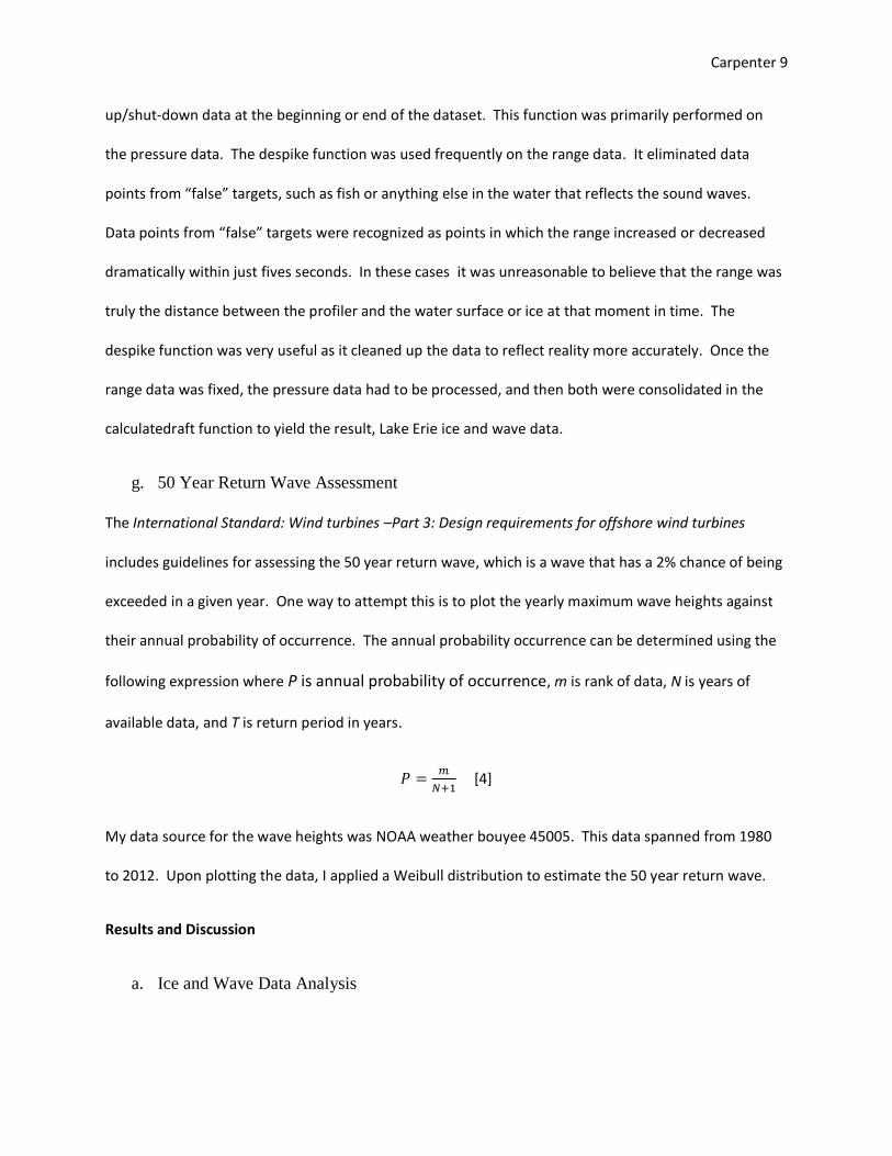
Below are plots of the three years of data from the SWIP. The x-axis represents time while the y-axis

represents a displacement in meters which can be interpreted as ice draft or wave amplitude. The

water level is 0 meters in all plots. The two features that appear throughout the data are ice and waves.

The rigid areas in the data with varying indents are ice while the smooth, fluid positive and negative

transitions are waves. The first large piece of ice appears around January 14th 2011 with a thickness of

about 1 meter. The data reveals a very large ice mass around January 17th. This 6 meter thick piece

seems unreasonable. It is possible that a keel of ice was forced vertical and then pushed further and

further down by collisions with other ice formations. The data from February 2011 reveals much more

reasonable ice thickness, fractions of a meter. By the middle of March the ice has melted andwaves are

present in April and May.

Carpenter 11

The time frame from December 2011 to March 2012 exhibits only waves. This was a relatively warm

winter that yielded little to no freezing. Some of the waves appear to reach amplitudes of 1.5 meters.

This is probably not realistic, however. During severe storms the lake floor soil gets stirred up and all of

the particulates can cause the instrument’s sonar to detect “false” targets.

Carpenter 12

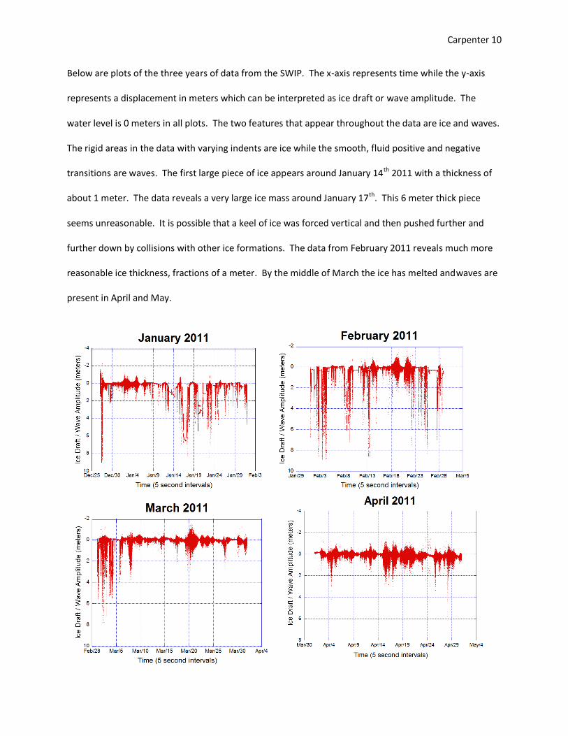
The next period of data shows waves in December 2012 and January 2013, then ice in February,

returning to waves in March and April. The max ice thickness in February is slightly over 1 meter. More

frequently the ice appears to be a fraction of a meter thick. There was about .2 meters of ice on the lake

on February 7th.

Carpenter 13

b. WERC Website

I was able to talk to Tom Seeber who added a research group webpage to Case’s website for my

research group, WERC, Wind Energy Research and Commercialization. In the future this website will be

accommodated with easily accessible, downloadable data. This could include data from the campus

turbine, the water intake crib, the two turbines in Euclid, etc. The data access will require username and

password. Not all parts of the website will be restricted though. A few pages may be dedicated to the

public for educational purposes. The web address is http://engineering.case.edu/groups/werc.

c. 50 Year Return Wave

Carpenter 14

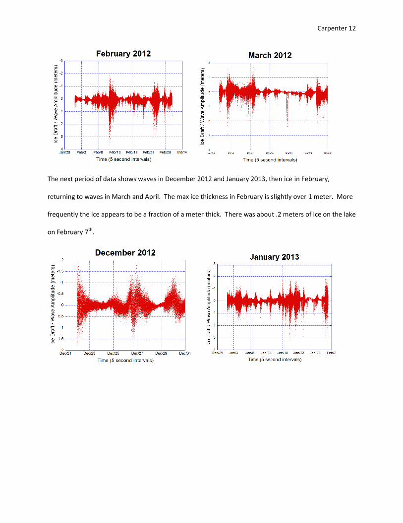
Below is a plot of the maximum wave heights each year. Notice the largest of these occurred most

recently in 2012 at 4.26 meters. 1995 and 1998 have the next largest wave heights.

Below is the plot of the annual maximum wave heights against their annual probability of

occurrence with the Weibull distribution applied. This distribution fit the data nicely so it was

reasonable to use it to predict the 50 year return wave. Since the 50 year return wave has a 2%

annual probability of occurrence, the corresponding wave height is 3.75m.

00.5

11.5

22.5

33.5

44.5

1980

1983

1986

1989

1992

1995

1998

2001

2004

2007

2010

Wav

e H

eigh

t (m

eter

s)

Year

Annual Max Wave Heights

-0.2

0

0.2

0.4

0.6

0.8

1

1.2

0 1 2 3 4 5 6

An

nu

al P

rob

abili

ty o

f O

ccu

ren

ce

Wave Height (meters)

Annual Maximum Wave Heights with Weibull Distribution

Weibull Distribution

50 year return wave

(3.75m, .20)

Carpenter 15

Summary or Conclusions

It was determined that the max ice sheet thickness from December 2010 through April 2013 was

slightly over 1 meter when ignoring the very large thicknesses which can be attributed to vertical

stacked pieces of ice. Typical thicknesses were a fraction of a meter.

The wave data showed waves reaching amplitudes of 1.5 meters on Lake Erie. This however is

not entirely true because severe storms can cause the amplitudes to be exaggerated in the data. More

frequently, the wave amplitude is .5 meters or below. The wave data was compared to historical

weather data and a correlation was present between high winds, storms, and large waves. Further, the

50 year return wave was determined by the Weibull distribution to be 3.75 meters.

These results encapsulate only a very small portion of the feasibility assessment of an offshore

wind turbine farm in Cleveland, so there is still much work to do in terms of studying external conditions

to better understand the structural needs of this project and potential issues that could arise.

Acknowledgements

I would like to thank REU SUR-WinD at Case Western Reserve University for accepting me into the summer 2013 program. Specifically, I would like to thank the two PI’s Dr. J. Kadambi and Dr. I. Alexander for this opportunity. I appreciate the guidance and assistance from my mentor Dr. Matthiesen and my graduate student assistant Daniel Corrigan throughout the summer. I would like to acknowledge Tom Seeber as he played a vital role in getting a research group website for WERC. Further, I give thanks to the City of Cleveland Division of Water for the trip to Cleveland’s water intake crib to check on the lidar. Lastly, I thank the National Science Foundation for the funding provided to this program.

References

[1] Stone, Matt, et al. SWIP Operators Manual. British Columbia, Canada: ASL Environmental Sciences Inc., June 2010. [2] IPS Processing Toolbox User’s Guide. British Columbia, Canada: ASL Environmental Sciences Inc., July 2011. [3] Great Lakes Wind Energy Center Feasibility Study. Cleveland, Ohio: juwi GmbH and its subsidiary JW Great Lakes Wind LLC, April 2009. [4] Makkonen, Lasse. NOTES AND CORRESPONDENCE: Plotting Positions in Extreme Value Analysis. Journal of Applied Meteorology and Climatology, 2005.