SUPREME SPLIT:

COMPARING THE ROBERTS AND REHNQUIST COURTS’ IDEOLOGICAL

PREFERENCES TOWARD BUSINESS ACCOUNTING FOR CASE SELECTION

Clifford Winston Jia Yan Quentin Karpilow

Brookings Institution Washington State University Yale University

CWinston@brookings.edu Jiay@wsu.edu Quentin.Karpilow@Yale.edu

Abstract. There is growing concern that Supreme Court rulings are increasingly being made along

partisan lines. We develop a new methodology that jointly analyzes justices’ selection of cases to

hear and their rulings, while allowing for justice preference heterogeneity, to estimate the effects

of their ideology on business case rulings in the Roberts and Rehnquist Courts. In contrast to prior

approaches that mute justices’ ideological preferences by not controlling for case selection, we

find strong evidence of growing politicization and polarization on the Supreme Court. We briefly

discuss explanations for, consequences of, and possible reforms to mitigate this worrisome trend.

May 2016

1

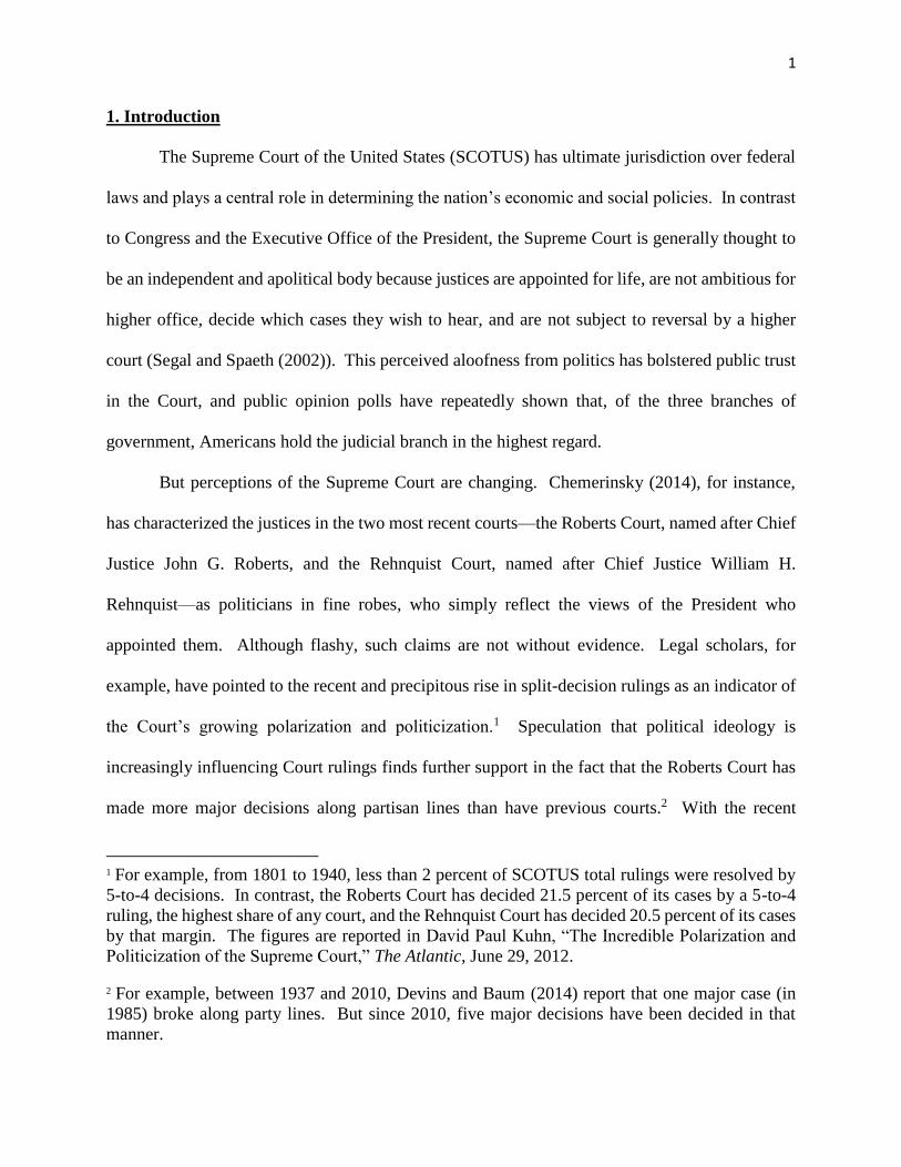
1. Introduction

The Supreme Court of the United States (SCOTUS) has ultimate jurisdiction over federal

laws and plays a central role in determining the nation’s economic and social policies. In contrast

to Congress and the Executive Office of the President, the Supreme Court is generally thought to

be an independent and apolitical body because justices are appointed for life, are not ambitious for

higher office, decide which cases they wish to hear, and are not subject to reversal by a higher

court (Segal and Spaeth (2002)). This perceived aloofness from politics has bolstered public trust

in the Court, and public opinion polls have repeatedly shown that, of the three branches of

government, Americans hold the judicial branch in the highest regard.

But perceptions of the Supreme Court are changing. Chemerinsky (2014), for instance,

has characterized the justices in the two most recent courts—the Roberts Court, named after Chief

Justice John G. Roberts, and the Rehnquist Court, named after Chief Justice William H.

Rehnquist—as politicians in fine robes, who simply reflect the views of the President who

appointed them. Although flashy, such claims are not without evidence. Legal scholars, for

example, have pointed to the recent and precipitous rise in split-decision rulings as an indicator of

the Court’s growing polarization and politicization.1 Speculation that political ideology is

increasingly influencing Court rulings finds further support in the fact that the Roberts Court has

made more major decisions along partisan lines than have previous courts.2 With the recent

1 For example, from 1801 to 1940, less than 2 percent of SCOTUS total rulings were resolved by

5-to-4 decisions. In contrast, the Roberts Court has decided 21.5 percent of its cases by a 5-to-4

ruling, the highest share of any court, and the Rehnquist Court has decided 20.5 percent of its cases

by that margin. The figures are reported in David Paul Kuhn, “The Incredible Polarization and

Politicization of the Supreme Court,” The Atlantic, June 29, 2012. 2 For example, between 1937 and 2010, Devins and Baum (2014) report that one major case (in

1985) broke along party lines. But since 2010, five major decisions have been decided in that

manner.

2

passing of Justice Antonin Scalia, there is concern that the Court will be deadlocked on a number

of major cases until a ninth justice is appointed and confirmed. Finally, Rishikof, Messenger, and

Jo (2009) show that Justices’ recent hiring of law clerks is also occurring much more along party

lines than in the past. Because those clerks play critical roles in selecting the petitions that the

Justices agree to hear and in drafting Justice opinions, the authors argue that such partisan hiring

practices have contributed to the Court’s polarized environment.3

While the circumstantial evidence presented above alludes to the growing politicization of

the Court, justice ideology is likely to be a potentially important influence on to SCOTUS

outcomes because SCOTUS justices are appointed for life and because their decisions are not

subject to reversal by a higher court. As a result, those policymakers enjoy greater freedom than

elected officials to allow their ideological preferences to influence their decisions. Moreover,

Posner (2008) argues that because Justices do not share a commitment to a logical premise for

making a decision (for example, cost-benefit analysis); they are ideological because they cannot

be anything else.

On the other hand, Rosen (2013) argues that, if justices based their decisions solely on their

ideologies, they could damage their reputations as fair justices, discredit the President who

appointed them, and possibly undermine the Court in the eyes of the public, which could lead to

3 The growing polarity of the Supreme Court is further suggested by Peppers and Giles’ (2012)

findings that the justices’ attendance at the President’s State of the Union (SOTU) address has

declined in recent decades and that a justice is more likely to attend the SOTU address if he or she

was appointed by the President giving the address. According to the authors, from 1965 (President

Johnson’s second address) to 1980 (President Carter’s last address), 84 percent of the justices

attended the SOTU address on average. From 1982 through 1999, the justices’ average attendance

declined to 56 percent. And since 2000, only 32 percent of the justices attended the address, with

Justice Clarence Thomas claiming that “it has become so partisan and it’s very uncomfortable for

a judge to sit there,” and Justice Antonin Scalia describing the annual address as “cheerleading

sessions.”

3

certain actions, such as term limits or even retention elections. It seems likely, then, that ideology

is an important, but not the only, factor shaping SCOTUS decision-making.

While the view that ideology influences SCOTUS outcomes is compelling, it is still an

empirical question as to whether stronger ideological preferences are making the Roberts Court

more polarized than previous courts. Chief Justice Roberts has, himself, acknowledged the policy

importance of this question, claiming that, if the Court were to adopt the extreme partisanship that

currently characterizes the other branches of the federal government, it would seriously damage

SCOTUS’s reputation among the public, as well as jeopardize the judicial nomination and

confirmation process. Accordingly, Roberts has sought to assuage concerns that the Court is

functioning as a political entity by publicly pledging to embrace Chief Justice John Marshall’s

conception of the judicial branch as a nonpartisan steward in a polarized democracy.4

Legal scholars who have attempted to determine systematically whether the Supreme Court

is becoming more polarized under Chief Justice Roberts are divided. For example, Chemerinsky’s

(2008) assessment of the Roberts Court after three years bemoans the new justices who have forged

a “solid conservative voting majority” and concludes that the Court is exceedingly pro-business,

while Adler (2008) disagrees and says the Court is only “moderately more conservative than it had

been immediately before” and is not notably pro-business. Adler points out that the smaller

number of case petitions that the Roberts Court accepted during the period suggests caution should

be exercised about making sweeping judgments about its ideological trajectory. Lee Epstein,

Landes, and Posner (2013a) performed a statistical analysis of business cases and concluded that

the conservatives on the Roberts Court are extremely pro-business and that the liberals are only

4 Justice Roberts’ concerns about polarization and partisanship in the Supreme Court are

summarized by Rosen (2013) and by Professor Geoffrey Stone of the University of Chicago Law

School in “Our Politically Polarized Supreme Court?,” Huffington Post Blog, September 24, 2014.

4

moderately liberal. Richard Epstein (2013) challenged their finding, stressing that the authors do

not control for potential selectivity bias in the case petitions that the Roberts Court accepts.

In this paper, we explore the influences of justice ideology in the Roberts Court by

analyzing the determinants of its rulings and the Rehnquist Court’s rulings on business cases. As

noted by Epstein, Landes, and Posner (2013a), business cases are useful to analyze because (1)

justices tend to have well-defined preferences toward business and the policies favored by most

business interests, and (2) justice political ideology (liberal or conservative) can serve as a good

proxy for those preferences, with conservative justices being more likely than liberal ones to make

decisions that favor business firms. Importantly, we isolate the effects of political ideology on

judicial rulings by developing a joint mixed-logit model that accounts for both justice preference

heterogeneity and the selection of petitions by SCOTUS.

To the best of our knowledge, this is the first application of a new methodology to correct

for selectivity bias when (1) discrete choice probability models are used to characterize both the

selectivity behavior (petition selection) and the outcome of interest (justices’ individual rulings for

or against a business entity), and (2) the selection error is correlated with the random coefficients

in the outcome model. Although it has long been argued that failure to control for case selectivity

can bias analyses of court outcomes (Priest and Klein (1984)), previous empirical studies of

SCOTUS rulings have not formally incorporated case selection decisions into an econometric

analysis.5 As a result, this paper contributes to the broader study of SCOTUS decision-making by

addressing a potentially critical, but largely ignored, source of estimation bias. In particular, a

5 For example, see: Epstein, Landes, and Posner (2013a, b); prediction models of Supreme Court

outcomes developed by Ruger et al. (2004) and Katz, Bommarito, and Blackman (2014); and

examinations of changes in individual justices’ ideological beliefs by Iaryczower and Shum (2012)

and Martin and Quinn (2007).

5

Court with strong ideological preferences may mask or exacerbate those preferences by agreeing

to hear more or fewer cases of a certain type (e.g., politically divisive cases). Our methodology

should also be of general interest, given the ubiquity of selection problems and discrete outcomes

that economists study. For example, instead of the classic Heckman selection problem of the

discrete selection choice of employment and a continuous wage outcome, one can think of the

selection problem of employment and a discrete outcome of earnings above the minimum wage.

We find that justices’ ideologies have a statistically and quantitatively important influence

on their rulings on business cases. Moreover, when we compare justices’ ideological preferences

in the Rehnquist Court with those in the Roberts Court and we implement our methodology to

control for case selection, we find strong evidence of growing politicization and polarity on the

Supreme Court. This finding holds even when we confine our analyses to those justices who have

served on both Courts. In contrast, we obtain much weaker evidence on growing politicization

and polarity if we do not control for case selection, indicating that the Roberts Court’ justices mute

their ideological preferences through the petition selection process. Thus, Supreme Court justices

have not moderated their ideological preferences over the past two decades; instead, those

preferences appear to have grown stronger and more divisive. We conclude by briefly discussing

the explanations for and adverse consequences of the Court’s growing polarity, as well as possible

reforms to mitigate this worrisome trend.

2. An Overview of the Determinants of Petition Selection and Case Outcomes

Two extreme theories about judges’ behavior exist (Edwards and Livermore (2009)). The

“legalist” theory asserts that judges mechanically apply the law to the facts, while the “political

6

science” theory argues that a judge’s political ideology has a predominant influence on his or her

rulings.

Epstein, Landes, and Posner (2013b) suggest a middle ground wherein ideology is a

component in judicial behavior that increases in influence as a judge moves up the judicial

hierarchy and gains more independence. In this framework, however, ideology does not rule out

other possible influences on judges’ rulings. We draw on this third approach to model two

SCOTUS decision-making processes: (1) the Court’s selection of petitions to hear (i.e., the

decision to grant a petition a writ of certiorari, or “granting cert”); and (2) justice rulings on

business-related cases that are heard by SCOTUS (i.e., case-outcome votes). We provide an

overview of the relevant influences and their measurement on those two decision junctures.

Case-Outcomes Model

Data on U.S. Supreme Court business case outcomes during the Rehnquist Court and the

Roberts Court up through 2011 are available in Epstein, Landes, and Posner’s (2013a) Business

Litigant Dataset (BLD). This dataset consists of all cases that were orally argued before the U.S.

Supreme Court and that involved a business entity as either a respondent or a petitioner, but not

both. Because BLD was constructed using Harold Spaeth’s well-known U.S. Supreme Court

Database, it contains detailed information on the legal characteristics, history, and outcomes of

Supreme Court disputes, as well as data on the votes of each Justice (Spaeth et al. (2014)). Due to

petition data constraints that are discussed in greater detail below, we limit our case outcomes

analyses to the 198 business cases that were submitted to and heard by SCOTUS between 1996

and 2011.

Following Epstein, Landes, and Posner (2013a), we classify any vote in favor of the

business litigant as “pro-business” and any vote in favor of the non-business party as “anti-

7

business.” Although it is possible for one company to win at the expense of the interests of the

larger business community, this classification scheme is superior to alternative definitions of a

“business win” because it is more transparent, relies less on the subjective coding judgments of

the researcher, and allows for the analysis of a wider range of business-related cases.6

We estimate separate models for the Roberts and Rehnquist courts to determine the distinct

ideological preferences of the justices on those courts. For each court, we initially follow Epstein,

Landes, and Posner (2013a) by specifying the probability of a pro-business vote as a function of:

(a) an indicator for each justice serving on the court, which captures the ideological preferences of

that justice;7 (b) an indicator of whether the lower court from which the case was appealed reached

a pro-business ruling; (c) a series of dummy variables indicating whether the Solicitor General

filed an amicus brief on behalf of the business litigant or the non-business litigant; (d) an indicator

of whether the federal government was the non-business party in the case; and (e) an indicator

variable of whether the substantive issues of a case fall within the scope of Spaeth’s “economic

activity” category. In an alternative set of specifications, we replace the individual justice

6 One popular definition of a business win focuses on cases that have been coded in the Spaeth

Database as being related to “economic activity,” and then uses Spaeth’s ideological classifications

of a case as either “conservative” or “liberal” as a proxy for pro- and anti-business decisions,

respectively. Epstein, Landes, and Posner (2013a), however, show that this definition excludes a

substantial number of cases that do not fall into the “economic activity” category, but nonetheless

involved business entities. Even more telling, the authors find that many of those excluded cases

were accompanied by an amicus curiae brief filed by the Chamber of Commerce, a sure indicator

of the business relevance of a case. In addition, Epstein, Landes, and Posner call into question the

accuracy of Spaeth’s ideological classification of cases when they conduct their own reanalysis of

147 business-related cases. Strikingly, in about 39 percent of the 147 cases reviewed, the authors

disagreed with Spaeth’s ideological coding. Rates of disagreement were even higher for businesses

cases that did not fall within the “economic activity” classification. 7 Note the dummy captures ideological preferences and not just disagreement among justices

because we control for several other factors on case decisions and because our main analyses

explore systematic differences among justices’ preferences by assessing them relative to the chief

justice’s preference.

8

indicators with a single ideology binary measure that identifies justices as either

Conservative\Moderate or Liberal according to Epstein, Landes, and Posner’s (2013b)

classification system, which they explain in detail in chapter 2 of their 2013b book. Importantly,

their methodology determines justices’ ideologies based on their actual votes in cases, as opposed

to the ideology of the President who appointed them. In addition, the ideological status of a justice

does not change over time.

Finally, as robustness checks, we expanded the specification of the case-outcomes model

to include: (f) eleven topical dummies that categorize petitions to the Supreme Court according to

the main legal questions and substantive matters of the dispute, which can be used to differentiate

between the subject matter of the business cases heard by the Court;8 and (g) a series of lower-

court dummies, which are described in greater detail below.

8 We use Bloomberg BNA’s Supreme Court Today’s dataset to obtain petitions to the Supreme

Court for each year of our sample. That database categorizes petitions according to 64 different

legal categories. Due to sample size issues, we aggregated those fine-grained classifications into

eleven broad topic categories, namely: (1) Criminal law, which contains cases related to criminal

law, prisons, and racketeering; (2) Civil rights law, which is composed of Bloomberg’s civil rights,

education, election, and employment discrimination topics; (3) Regulatory law, which contains

petitions related to agriculture, antitrust, energy, environment, health care, international trade,

securities, utilities, telecommunications, and transportation; (4) Consumer and worker safety law,

which contains Bloomberg’s consumer credit, consumer protection, deceptive trade, employee

benefits, mining, occupational safety, product liability, unfair trade practices, employment/labor,

attorney ethnics, and torts topics; (5) Private/state business law, which contains petitions related

to accounting, banking/finance, contracts, corporate and business law, insurance, partnerships,

arbitration, alcoholic beverages, and gambling; (6) Intellectual property law, which is composed

of Bloomberg’s copyrights, patents, and trademarks topics; (7) Government authority issues,

which contains petitions related to administrative law, agency law, international law, takings,

appellate procedure, civil procedure, congressional operations, evidence, judicial appointments,

and constitutional law; (8) Technology issues, which contains petitions related to cyber law, media,

and privacy; (9) Other government issues, which is composed of Bloomberg’s bankruptcy,

government contracts, immigration, infrastructure, maritime, military, Native American, postal

services, social security, veterans, and freedom of information topics; (10) Tax law, which is

composed only of Bloomberg’s tax topic; and (11) Private non-business, which includes

Bloomberg’s family law, trusts and estates, and nonprofit organizations topics.

9

Petition Selection Model

In principle, there are two selection decisions that may be relevant for our analysis: The

SCOTUS justices’ selection of cases from the pool of lower court appeals and the selectivity

behavior of litigants to include their case in the pool of SCOTUS petitions. Assembling a data set

and estimating a model of the petition decisions by litigants would be a very formidable task of

questionable value to our analysis given: (1) all litigants who lose at lower courts have the right to

petition the Supreme Court to hear their case; and (2) many business litigants take advantage of

this right, especially because the cost to those litigants of submitting a petition is not high.

Moreover, we are not aware of any theoretical or empirical evidence that there is any systematic

bias in the cases that business litigants choose to appeal, and, given that we are comparing the

Roberts Court (2005-2011) to the latter half of the Rehnquist Courts (1996-2005), we limit the

possibility that differences in the types of cases that make it into the SCOTUS pool of petitions

are driving our results. In particular, it seems highly unlikely that the types of cases being

processed by the lower courts during the end of the Rehnquist Court are categorically different

than those circulating through the lower courts during the Roberts Court.

Thus, we focus on estimating the determinants of case selection by the Roberts and

Rehnquist Courts using the online Bloomberg BNA Supreme Court Today dataset.9 The

Bloomberg database contains a myriad of information on virtually all paid cert. petitions filed with

the Supreme Court between 1996 and 2011.10 However, because the format of the database is not

9 http://www.bna.com/supreme-court-today-p5946/

10 Paid cert. petitions are also called non-pauper petitions. No one has collected data on pauper

(non-paid) petitions, which represent only about 10% of the Supreme Court’s docket and tend to

be easily resolved by the justices (Posner (2008)). Note that some early-1996 paid cert. petitions

10

conducive to statistical analysis and because data must be downloaded separately for each

individual petition, gathering information on the more than 27,000 petitions submitted during this

time period proved to be logistically infeasible. We therefore constructed a sample of 2768

petitions that were randomly selected from the Bloomberg database.11 In addition, the 198 cases

in our Business Litigant Database that are used to estimate the case-outcomes model can be treated

as a choice-based sample in estimating the petition-selection model. Although the petition-

selection model can be estimated using the random sample of 2768 petitions, combining the

random sample with the choice-based sample can improve the efficiency of the parameter

estimates. Hence, we estimate our model with the random sample and then combine it with the

choice-based sample as a robustness check.

We are not aware of a previous Supreme Court petition selection model that explains how

the justices select petitions, although it is known that a petition needs four justice votes to be

selected, the court typically hears about 1 percent of the nearly 9,000 appeals that they receive

each year, and that it is customary for the court’s decision on whether to hear a case does not

indicate how individual justices voted.12 Thus, we reviewed the extant literature on the factors

are also missing from the Bloomberg database. The database does, however, contain the full

population of non-pauper SCOTUS petitions submitted in all post-1996 years. 11 To construct our random sample of Bloomberg petitions, we first sorted eligible petitions by the

date on which the SCOTUS decided to hear (or not hear) the petition. Only petitions that were

either granted or denied a hearing with SCOTUS were eligible for selection. Then, for each year,

we selected every tenth petition to include in our sample, meaning that, on average, we sampled

between 100 and 300 petitions for each SCOTUS term. Note that the 2768 randomly selected

petitions and the 198 BLD petitions are not mutually exclusive because some randomly selected

petitions were also included in the Business Litigant Dataset. 12 Jeffrey L. Fisher, “The Supreme Court’s Secret Power,” New York Times, September 25, 2015

argues that justices’ votes on each petition should be announced to increase transparency on why

justices pick the cases they do. The absence of this voting information makes it difficult for us to

assess whether justices engage in “defensive denials” or other forms of strategic behavior (Corday

and Corday (2008)).

11

that are most relevant for explaining the Justices’ case selection decisions and specified the

probability that a petition is granted a hearing with the Supreme Court as a function of: (a) thirteen

lower court indicators and a reference category that identify the court system whose decision is

being appealed;13 (b) a lawyer quality dummy that indicates whether any of the lawyers filing the

petition are “top Supreme Court advocates,” which we define to be litigators who have argued at

least ten cases before the Supreme Court by 2010;14 (c) a second lawyer performance dummy that

identifies top Supreme Court advocates who were working as the U.S. Solicitor General when the

federal government filed the petition; (d) an indicator for whether the Court invited the Solicitor

General to submit a brief analyzing the petition and expressing the views of the United States;15

(e) a series of Court-calendar dummies indicating whether the decision to grant or deny a petition

was made during the Court’s summer recess, the May or June lists, or one of the seven argument

13 More specifically, we include separate dummies for (a) each of the eleven circuit courts of

appeals; (b) the District of Columbia circuit court (indicated in the estimations as lower court

dummy12); and (c) the Federal Patent Court (indicated in the estimations as lower court dummy

13). The reference category includes petitions from state and lower district courts, as well as any

court not explicitly identified by our set of indicator variables. 14 Biskupic, Roberts, and Shiffman (2012) and Lazarus (2008) argue that SCOTUS grants petitions

filed by certain top advocate lawyers at a significantly higher rate than they grant petitions filed

by other lawyers. While the Bloomberg database provides the names of the lawyers filing a

petition, we relied upon data published by Bhatia (2012) to identify top Supreme Court Advocates.

Specifically, Bhatia ranks modern lawyers according to the number of SCOTUS cases they have

argued between 2000 and 2010, as well as provides lifetime numbers of Supreme Court

appearances for each of those lawyers. Taken together, the Bloomberg and Bhatia data allowed us

to identify petitions filed by lawyers who, as of 2010, had argued at least 10 cases before the

Supreme Court. 15 Thompson and Wachtell (2009) discuss the close relationship that solicitor generals have with

the Supreme Court and the Court’s requests for their views on petitions.

12

sessions;16 and (f) a count variable measuring the size of the Supreme Court’s docket in a given

year.17

3. Econometric Model

We now develop a new econometric model to estimate the effects of the ideological

preferences of the Roberts and Rehnquist Court justices on the outcomes of business-related cases,

accounting for the non-random selection of petitions. We let index the two courts, with

for the Rehnquist Court and for the Roberts Court. For a given case before court , there

are up to nine votes by the justices on that court. We let denote the vote of justice on case

, with equal to 1 if the vote is pro-business and 0 otherwise. Thus the justice case outcomes

vote under court g is given by the following binary response model:

, (1)

16 Corday and Corday (2004) discuss how the volume of petitions affects the likelihood of whether

the Supreme Court will agree to hear a case. The Supreme Court term begins the first Monday in

October and consists of seven argument sessions during which the Justices hear cases and deliver

opinions; the May and June lists during which the Court sits only to announce orders and opinions;

and the summer recess during which the Court’s only duty is to review newly-submitted petitions

and make preparations for the fall argument sessions. Following Cordray and Cordray (2004),

petition decisions announced in July, August, September, and the first Monday of October were

assigned to the summer recess; subsequent petition decisions made in October (but after the first

Monday) were assigned to the October session, the first of the seven argument sessions. Month

dummies were then constructed to identify the six remaining argument sessions (November

through April) and the May and June lists. 17 Annual docket size was measured as the total number of petitions filed during the year plus the

total number of cases remaining on the docket from the previous year. Note that these counts

include both the non-pauper petitions recorded in the Bloomberg dataset and the much smaller

number of pauper cases. Data on docket size come from the Federal Judicial Center

(http://www.fjc.gov/history/caseload.nsf/page/caseloads_Sup_Ct_totals).

g 1g

2g i g

ijy j i

ijy

0* g

ij

g

i

C

j

g

i

L

j

g

iijij eDDyIy BX

13

where is an indicator function that is equal to 1 if the inside argument is true and is equal to

zero otherwise; is a liberal (or moderate) L ideology and is a conservative C ideology

dummy for justice ; and is a vector of exogenous influences on the case outcome discussed

previously, B is a vector of parameters, and e is an error term.18

The justices’ ideological preferences toward a case, captured by the parameters and

, would be expected to vary across cases because cases have different characteristics, many of

which are unobserved. Given that there are at most 9 votes for a case, it is infeasible for us to use

fixed effects by interacting case dummies with ideological dummies to control for the variation in

the ideological preferences across cases. We therefore adopt a random-effects specification and

model and as two correlated random coefficients; as noted later, the joint distribution of

the two random coefficients is allowed to be correlated with the case selection process because

unobserved case characteristics may affect both ideological preferences and case selection.

Because we include an intercept in the specification, the mean of is normalized to

zero and can be written as , where denotes a random term with zero mean.

Given this specification, the estimates of measure for a given court the average pro-business

bias of liberal or moderate justices compared with the pro-business bias of conservative justices.

Selectivity Bias

A probit or logit regression to estimate equation (1) suffers from sample-selection bias

because estimation is based only on the cases that the Supreme Court agreed to hear and ignores

18 We initially estimate separate dummies each justice and we then perform estimations where we

aggregate and specify liberal/moderate and conservative ideology dummies for each justice. Our

derivation also holds for the first approach.

I

LjD C

jD

j iX

g

ig

i

g

ig

i

g

i

g

ig

i

gg

i g

i

g g

14

the information provided by the cases that the Court declined to hear. Let denote the binary

indicator for case selection, which is equal to 1 if case is granted a hearing by the Supreme Court

and 0 otherwise. Thus, the case selection model under court is specified as:

, (2)

where is a vector of observed exogenous influences on case selection discussed previously

(some of which are not included in ), δ is a vector of parameters, and ν is an error term.

Formally, the selectivity issue arises because we can observe a case outcome only when

:

. (3)

The random coefficients in equation (1), and , are likely to be correlated with the error

term, , because unobserved case characteristics that affect case selection also affect how

justices’ preferences are revealed in the merits-ruling stage of the process. Thus maximizing the

log-likelihood of the unconditional probability as a probit or logit estimation with

random coefficients leads to inconsistent parameter estimates.

If we assume joint normality of , and , such that

, (4)

where and , and if the latent variable is observable, we can specify

the conditional expectation function

, (5)

is

i

g

0* gi

giii vsIs δZ

iZ

iX

ijy

1is

0 0Pr11Pr ** iijiij sysy

g

ig

i

gi

0Pr * ijy

g

ig

igi

g

i

g

i

gg

i

g

ii v μθΓ

,

22,0~ Ng

iμ 1,0~ Nvgi

*ijy

g

iii

g

j

g

i

L

j

g

iij vvEDsyE δZθDBX 1*

15

where . It would appear that equation (5) can be estimated to obtain consistent

parameter estimates by the usual two-step control-function type approach (Heckman (1976)): first

estimate a probit selection model to obtain the inverse-mills ratio and then regress on the

explanatory variables along with interactions of the inverse-mills ratio and the ideological

dummies to control for the unobserved influences on selection. However, that approach cannot be

applied here because we observe only the binary case outcome . Given the joint normality

assumption in equation (4) and the condition given by equation (3), we have

(6)

The last inequality is the result of Jensen’s Inequality because the indicator function is nonlinear.

Since we cannot use the standard two-step approach to control for selectivity bias, we instead

derive the joint distribution of the endogenous variables , where , and we

estimate the parameters in equation (1) by Maximum Simulated Likelihood Estimation (MSLE).

This appears to be the first application, to the best of our knowledge, of a new methodology to

correct for selectivity bias when both the selectivity and outcome equations are discrete. We

extend this application to allow the selection error to be correlated with the random coefficients in

the outcome model.

C

j

L

jj DD ,D

*ijy

ijy

11

g

ij

e

g

i

g

i

g

ij

gg

i

g

i

g

ij

g

i

L

j

gg

ij

g

ij

e v

g

i

g

i

g

i

g

i

g

i

g

i

g

ij

gg

ij

g

i

L

j

gg

ij

iij

eddfvvEDeI

dedvvvfdfvDeI

syP

gij

gi

gij

gi

gi

u

u

uuuDθδZDBX

δZuuuDθDBX

ii sP ,y 91,..., iii yyy

16

We identify the case outcome model with selectivity by assuming the distribution of ,

and is joint normal.19 Dropping the court superscript to simplify the exposition yields:

;

(7)

is assumed to have a logistic distribution with variance normalized to .

To summarize, then, our econometric model consists of: two binary response models, a

binary probit model of petition selection and a binary mixed-logit model of pro-business voting on

cases selected by SCOTUS; a cross-model correlation that is represented by equation (7);

correlations among different justices’ votes on a case that are captured by random individual

effects, and , and their correlation; and justice ideological preferences that influence case

outcomes that are allowed to vary, as indicated by equation (7), according to unobserved case

characteristics that affect both case selection and case outcomes.

Deriving the Data Likelihood

19 Heckman and Singer (1984) propose a nonparametric maximum-likelihood approach that uses

a discrete type distribution for the random components in an econometric model. Their approach

is difficult to apply to our sample selection model with random coefficients because we show in

equation (9) below that the data-likelihood of the sample selection model requires knowledge of

both the joint distribution and the conditional and marginal distributions of iii ,, . Although

we can use a common random component with a discrete type distribution to capture the

correlation of iii ,, , it is not possible for us to derive marginal and conditional distributions

from such a specification. Thus, assuming joint normality provides a tractable and plausible way

to identify the sample selection model.

g

i

g

igi

Ω0ΩΩ

Ω00 ,

1,

1

,~,,2212

12

2

32

3

2

1

21

MVNMVNMVNiii

ije 32

i i

17

After dropping the court superscript, we define and . For any

case in the Business Litigation Database, the joint distribution of and can be

expressed as

. (8)

Note, we assume that , where indicates the standard normal

distribution function.

The conditional probability is given by

i i

i i

i

i

iiiiiii

j

ijiiiij

iiiiiiiijiiii

iiiiijiii

iiiijiiijiii

dfdfsyP

dfdfsP

dfsP

dsfsPsP

δZΓΓΘDΓW

δZΓΓΘDΓWy

δZΘDWy

ΘDWyΘDWy

Γ

Γ

,,,,,1

,,,,,1

,,,,1

1,,,,1,,,1

(9)

where given our mixed logit specification, ΘDΓW ,,,,,1 ijiiiij syP has a simple binary logit

functional form. According to the specification (7), iif Γ is a bivariate normal density. The

density function is a truncated normal that is truncated below (because

). When sample selection is not correlated with the case outcome equation, the integration

in (9) does not depend on because . In that case, the parameters in the case

outcome equation can be estimated consistently by maximizing the log of the likelihood function

defined in (9).

Estimation

iii ZXW , δΩBΘ ,,,

i 91,..., iii yyy is

δZΘDWyΘDWy ,1,,,1,,, iijiiijiii sPsPsP

δZδZ iiisP ,1

ΘDWy ,,,1 jiii sP

δZiiif δZi

1is

i iii ff ΓΓ

18

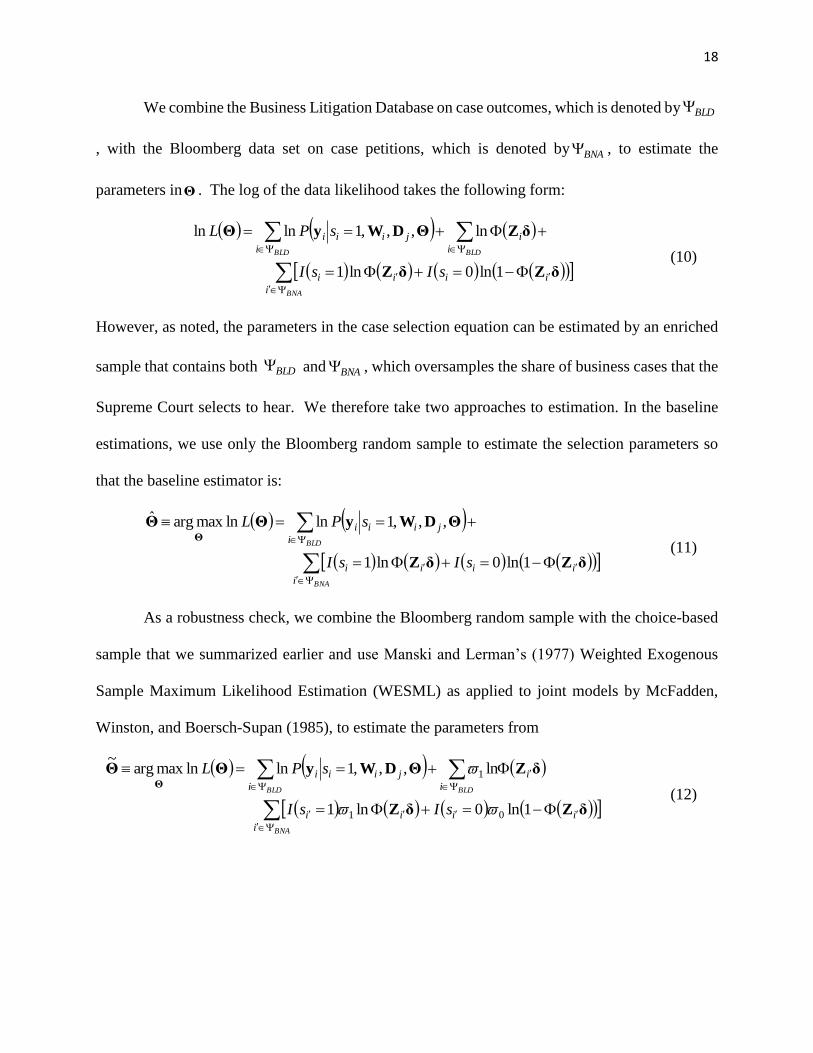
We combine the Business Litigation Database on case outcomes, which is denoted by

, with the Bloomberg data set on case petitions, which is denoted by , to estimate the

parameters in . The log of the data likelihood takes the following form:

(10)

However, as noted, the parameters in the case selection equation can be estimated by an enriched

sample that contains both and , which oversamples the share of business cases that the

Supreme Court selects to hear. We therefore take two approaches to estimation. In the baseline

estimations, we use only the Bloomberg random sample to estimate the selection parameters so

that the baseline estimator is:

(11)

As a robustness check, we combine the Bloomberg random sample with the choice-based

sample that we summarized earlier and use Manski and Lerman’s (1977) Weighted Exogenous

Sample Maximum Likelihood Estimation (WESML) as applied to joint models by McFadden,

Winston, and Boersch-Supan (1985), to estimate the parameters from

(12)

BLD

BNA

Θ

BNA

BLDBLD

i

iiii

i

i

i

jiii

sIsI

sPL

δZδZ

δZΘDWyΘ

1ln0ln1

ln,,,1lnln

BLDBNA

BNA

BLD

i

iiii

i

jiii

sIsI

sPL

δZδZ

ΘDWyΘΘΘ

1ln0ln1

,,,1lnlnmaxargˆ

BNA

BLDBLD

i

iiii

i

ii

jiii

sIsI

sPL

δZδZ

δZΘDWyΘΘΘ

1ln0ln1

ln,,,1lnlnmaxarg~

01

1

19

where , and is defined similarly to

reweight the cases not selected by the Supreme Court. This estimator yields consistent parameter

estimates.20

Estimation of the model requires evaluating the log-likelihood function given by equation

(11) or the pseudo-log-likelihood function given by equation (12) at each iteration of the

optimization procedure.21 In those functions, the conditional probability ,

which is given in equation (9), can be evaluated only numerically because the probability involves

integrations with respect to both given and itself. We use Monte-Carlo integration to

approximate the probability, where the Monte-Carlo approximation to equation (9) is given by

(13)

where represents the th random draw of from the truncated normal distribution

and represents the th random draw of from the bivariate normal

distribution conditional on – . and are the total number of

random draws for and respectively.

20 The WESML estimator is consistent but not efficient because the shares are determined from

data instead of being estimated following an approach developed by Cosslett (1981). However,

we found it computationally difficult to simultaneously estimate both the model parameters and

the sampling weights.

21 We use the term pseudo-log-likelihood function because we are not taking Cosslett’s (1981)

approach to obtain efficient estimates by maximum likelihood estimation. Vossmeyer (2015)

suggests a Bayesian approach that could be used to estimate the model.

Sample enriched in the hearing granted cases of %

Sample Bloomberg in the hearing granted cases of %1 0

ΘDWy ,,,1 jiii sP

iΓ i i

R

r

R

r j

j

r

i

r

iiijjii yPRR

P1 1

9

1

,,,11

,, ΘDΓWΘDWy

r

i r i

1,0, δZiTN r

i

r

iΓ r iΓ

r

i 12122212, ΩΩΩΩ r

iN R R

i iΓ

20

The computational burden of evaluating equation (13) is considerable because of the

nesting structure in the Monte-Carlo integrations. To reduce computation time, we used the Halton

sequence (Train (2009)) to simulate random draws when we implemented the integrations. The

estimation results we report are based on 150 Halton draws; we performed robustness checks on

the base-line results in table 4 by increasing the number of draws to 300 and we found that the

results changed very little.

4. Identification

We seek to estimate the joint probabilities of Supreme Court Justices’ votes on a case and

whether a case is selected by SCOTUS. Because we cannot exploit a natural or quasi-natural

experiment to estimate the joint probabilities, we identify the probabilities by excluding from the

case-outcomes model predictors of petition selection that are uncorrelated with the justices’ rulings

on the merits. We provide a careful institutional justification for the exclusion restrictions that is

informed by the legal literature, and we perform robustness checks by estimating alternative

models that relax some of those restrictions. Below, we discuss the factors that we assume are

orthogonal to justice voting on the case merits.

Monthly Calendar Dummies and Docket Size

Monthly calendar dummies and docket size capture the impact of changes in the Justices’

workload on their petition decisions. During the past several decades, the volume of Supreme

Court petitions has steadily risen from about 2,000 petitions in 1960 to a little under 9,000 in 2012

(Federal Judicial Center (2012)). The task of processing thousands of petitions each year places a

21

clear and substantial burden on the Justices and their law clerks, and legal scholars have

documented a variety of ways in which petition volume has affected both the quality of judicial

review and the composition of cases ultimately heard by the Supreme Court.22

Particularly relevant to our analysis are the findings of Cordray and Cordray (2004), which

indicate that cert-acceptance rates are dramatically lower during the summer recess and the months

of February and March. This variation cannot be explained by systematic differences in case

characteristics, because petitions must be filed within 90 days of the lower court ruling and there

is no reason to suspect that lower-court decisions on more meritorious cases are more likely to

occur in certain months of the year. Furthermore, once the appeal is filed, the highly structured

and largely automated process of reviewing and disposing of petitions leaves little room for

manipulation (either by the Justices or by the contestants involved), meaning that the assignment

of petition decisions to calendar months is largely a random process.23

22 Qualitative research, for instance, suggests that the Solicitor General’s Office typically drops a

non-trivial number of cert-worthy petitions based on their perceptions of the Court’s workload for

that year (Griswold (1975)). 23 Once a petition is submitted, the respondents have 30 days to file a brief in opposition. If they

choose to submit a brief in opposition, the respondents can file for an extension (typically another

30 days). If the respondents waive their right to file a brief in opposition or if the 30-day response

period expires, the petition is then circulated among the Justices' chamber the next time a

conference list of petitions goes out. New conference lists are circulated on a weekly basis and

the Court is scheduled to meet on pre-specified dates to discuss the petitions on each conference

list. If the respondents file a brief in opposition, the Court waits approximately 10 days in order

to allow the petitioner to file a reply, after which time the case is appended to the next conference

list. Occasionally, when respondents fail to submit a brief in opposition, the Justice will instruct

the respondents to prepare and file a brief in opposition within the next 30 days. On rare occasion,

the Court will also invite the Solicitor General to file an amicus curiae brief expressing the views

of the United States regarding whether the petition should be heard. Decisions on petitions may

also be postponed until the subsequent conference if Justices need more time to consider the case.

Such delays are rare, however, as the average time from submission to disposition of a petition is

only six weeks (Public Information Office of the Supreme Court of the United States (2014)).

Nelson (2009) provides more details on the petition-review process.

22

The observed monthly variation in cert-acceptance rates appears to be driven by work

pressures that arise from the structuring of the Court’s calendar. For instance, the Justices’

workload peaks in February and March, when they are scheduled to not only hear a full set of

arguments, but also to write their opinions for all the cases heard in the first four sessions of the

term. At the same time, incentives for granting new petitions reach an annual low in February and

March, primarily because January is the last session during which new cases can be added to the

Court’s docket for the current term, and the Justices have ample time to fill up next term’s

argument docket. Similar “institutional” forces can also explain the negative downturn in grant

rates during the summer recess.24

In sum, the month dummies and docket size variable primarily capture the effects of

exogenous resource constraints and idiosyncrasies in the Court’s schedule on petition selection.

Clearly, those influences do not affect the pro-business voting tendencies of justices on specific

cases and they are unlikely to be correlated with unobserved influences on case-outcome votes.

Top Advocate Dummy and Indicator for Whether the Solicitor General is the Petitioner

Court resource constraints also justify our assumption that the top advocate dummy and

the indicator of whether the Solicitor General (SG) is the petitioner are purely exogenous

influences on petition selection. Because Justices must review thousands of petitions each year,

24 In particular, Cordray and Cordray (2004, p. 209) explain that, “During the summer recess, the

Court acts on almost no petitions for certiorari, and thus allows three months of filings to

accumulate for disposition en masse upon their return in the fall. As a result, in each of the nine

terms we canvassed from 1996 to 2002, the Court dealt with, on average, more than 1,600 petitions

for certiorari at the end of the summer recess, as compared to an average of 574 petitions during

each of the other periods.” The authors hypothesize that the Justices may “feel” like they are

accepting large numbers of cases (even though their acceptances rates are strikingly low), or that

the overwhelming volume of cases has a “numbing effect” on the Justices and their law clerks. A

similar “overload effect” may be contributing to the low grant rates in February. The authors note

that the Justices consider about 50% more petitions in February than in the average session—an

increase that they attribute to the abnormally long recess that precedes the February session.

23

they have limited time to devote to any given petition.25 Consequently, Justices look to a variety

of indicators to determine the importance of a petition and whether it should be approved. One

“marker” of quality and legal significance is whether the petition was submitted by the Solicitor

General, SG (Cordray and Cordray (2008)). Due to the nature of the SG’s client (i.e., the United

States), writs for certiorari from the SG’s Office generally merit the attention of the Supreme

Court. In addition, as pointed by Cooper (1990), the Justices have confidence in the quality of

those petitions because the SG’s Office has a reputation for rigorously screening and vetting its

petitions, and because the Solicitor General is a repeat player before the Court. Days (1994)

provides a history of the Office and stresses that it enjoys a tradition of independence and that the

Solicitor General is not a “hired gun,” but is ultimately responsible for advancing the “interests of

the United States,” which may, on occasion, conflict with a governmental entity.

A similar argument helps explain why SCOTUS grants petitions filed by certain seasoned

Supreme Court advocates (many of whom were formerly employed in the SG’s Office) at a

significantly higher rate than they grant petitions filed by other lawyers. Lazarus (2008) reports

that the Justices’ clerks pay special attention to the petitions filed by prominent Supreme Court

advocates because their reputations as top litigators convey an important message about the

significance of the legal issues being presented and the credibility of the assertions being made.

Thus, much in the same way that the Solicitor General’s petitions carry an experience-based stamp

of quality assurance, the name of a top Supreme Court advocate on a petition acts as a beacon of

potential cert-worthiness that helps distinguish it from the thousands of other competing appeals.

25 Hart (1959), for example, estimated that SCOTUS Justices in the late 1950s could spend at most

twenty minutes reviewing each nonfrivolous petition, while Chief Justice Hughes reported that his

Justices were unable to spend more than four minutes discussing each petition at conference

(Cordray and Cordray (2004)). Finally, Lazarus (2008) explains that the Justices do not read a

large portion of petitions and, at most, read the memoranda prepared by the clerks.

24

Of course, it is possible that the high acceptance rates for SG and top-advocate petitions

are driven, in part, by political considerations. If, for example, the Court has a pro-business

orientation, but the current U.S. administration is enacting more private-sector regulations, then

the Justices may actively seek out SG petitions to limit the scope of government regulation.

However, because we include in our case-outcomes model an indicator for whether the federal

government was a party in the case, we largely control for potential correlations between the SG-

petitioner dummy in our petition-selection model and the error term in our case-outcomes model.26

Indicator for whether the Court Invited the Solicitor General to Submit a Brief Analyzing the

Petition and Expressing the Views of the United States

On rare occasions, the Court will solicit the perspective of the SG’s Office on the cert-

worthiness of a petition through a call for the views of the Solicitor General (CVSG). Extant

research suggests that the CVSG is another information-gathering tool that the Court uses to take

advantage of the SG’s independence and objectivity (Days (1994), and unmatched expertise in

federal policy and complex regulatory matters. For example, Thompson and Wachtell (2009) find

that 91% of the CVSG cases reviewed between 1997 and 2004 involved complex regulatory and

statutory schemes, while only 7% involved significant issues of constitutional law. This statistical

breakdown is consistent with the Justices’ competence in dealing with questions of

constitutionality, their relative unfamiliarity with regulatory systems, and the SG’s obvious

comparative advantage in advising the Court on issues related to federal regulation. The authors

also observe that, although the SG’s response to a CVSG is almost always accompanied with a

26 When we included the top Supreme Court advocate dummy in the case outcomes model, its

coefficient was statistically insignificant and the estimates of the model’s other coefficients were

barely affected.

25

suggestion for how the Court should rule on the case (assuming the petition is accepted), the

Court’s ultimate decision on the merits is uncorrelated with the SG’s recommendations. Finally,

Thompson and Wachtell point to a plethora of anecdotal evidence that decouples the CSVG from

any political motivations, further supporting our treatment of the CSVG indicator as exogenous to

the final votes in our case-outcomes model. 27

Lower-court Dummies

It is well-known that the Supreme Court is particularly prone to reverse the rulings of

certain appellate courts—most notably, the Ninth Circuit and the U.S. Court of Appeals for the

Federal Circuit on patent disputes.28 Prominent explanations for high reversal rates include

ideological differences between lower-court judges and Supreme Court Justices, as well as

variation in circuit size.29 Notable differences in the subject matter and the number of cases

disposed by circuit courts have also been documented (Hofer (2010)), and this variation may

account for part of the variation in cert-approval rates across appellate courts.

27 Specifically, Thompson and Wachtell quote Justice Ginsberg as saying: “The Solicitor acts as a

true friend of the Court when we call for its views on a case in which the United States is not a

party.” They also point to the following quote from former Solicitor General Lee: “The Solicitor

General’s office provides the Court from one administration to another with advocacy which is

more objective, more dispassionate, more competent, and more respectful of the Court as an

institution than it gets from any other lawyer or group of lawyers.” 28 The Ninth Circuit has been called the “rogue circuit” due to the high reversal rates of its rulings

by the Supreme Court. In addition, Tony Mauro, “Key Patent Dispute Divides Supreme Court

Justices,” National Law Journal, October 15, 2014 reports that SCOTUS has an unspoken distrust

of the U.S. Court of Appeals for the Federal Circuit as the ultimate arbiter of patent disputes

because this circuit court frequently reverses trial judge findings; thus, SCOTUS steps in to reset

the balance. 29 Larger circuits tend to have greater difficulties in maintaining “uniform law” (aka, consistency

in decisions across judges) within the circuit, which would account for the observed positive

correlation between circuit size and SCOTUS reversals of lower-court rulings (Scott (2006)).

26

Although variation in cert-grating rates may, in part, be due to the policy preferences of

SCOTUS justices, it is important to note that we control for whether the lower court’s ruling on a

case was pro-business in our case-outcomes model. This, in turn, enables the lower-court dummies

in our petition-selection model to capture cert-granting factors that are unrelated to the pro-

business inclinations of the Supreme Court Justices. As a robustness check, however, we include

the lower-court dummies in an alternative specification of our case-outcomes model.30

5. Estimation Results

Descriptive information about the voting behaviors of the Supreme Court justices provides

some initial insights into their ideological preferences. In table 1, we break down the Rehnquist

and Roberts Court justices’ votes on the 198 cases in the Business Litigant Database that were

granted a hearing with the Supreme Court between 1996 and 2011. There is a clear ideological

divide in the Rehnquist Court justices’ preferences: the share of liberal justices’ (Souter, Stevens,

Ginsberg, Breyer) votes that are pro-business is almost uniform at 37 percent, while the share of

moderate and conservative justices’ (Kennedy, Scalia, Thomas, O’Connor, Rehnquist) votes that

are pro-business is at least 48 percent. The ideological divide grows in the Roberts Court, with

30 It is worth noting that the petition-selection model does not control for circuit splits, which occur

when appellate courts generate conflicting rulings on a particular legal issue. Although the

Supreme Court is substantially more likely to grant cert in cases that create circuit splits, data on

circuit splits are sparse, largely because identifying such cases would require reading and

comparing thousands of appellate judicial opinions. However, the absence of a circuit split

variable does not pose a problem for our model because the lower-case dummies broadly capture

a circuit’s tendency to diverge from other appellate courts on questions of law. For example, the

high reversal rates of Ninth Circuit holdings partially reflect the Ninth Circuit’s heightened

probability of splitting with other appellate courts on legal issues. In addition, because nearly all

cert-worthy cases involve circuit splits, circuit splits are unlikely to be correlated in a meaningful

way with Supreme Court rulings on the merits. Thus, omitting circuit splits from the petition

model should not affect the consistency of the estimates in the model.

27

four of the five liberal justices voting pro-business less than 44 percent of the time (Kagan’s share,

which is based on a relatively small number of votes, is an outlier at 55 percent) and four of the

five conservative justices voting pro-business in more than 60 percent of relevant cases (Roberts’

share is 57 percent).

Table 2 shows that the justices’ ideological preferences have continued to diverge since

Elena Kagan joined the Roberts Court in 2010, as the incidence of pro-business voting among

conservative justices (82 to 91 percent) rose to nearly twice the rate among liberal justices (46 to

56 percent). Of course, these descriptive data do not account for differences in the cases that the

Rehnquist and Roberts justices heard, differences in the cases that the Roberts Court has heard

since 2010, or other non-ideological influences on the justices’ voting behaviors. Our econometric

model controls for those effects on the justices’ votes, thus enabling us to provide a more accurate

characterization of the justices’ ideological preferences and how they have evolved.

Case Outcomes and Petition Selection Models

We estimate separate models of case outcomes and petition selection and then present

estimates of the joint model of those decisions to show the effects of controlling for case

selectivity. Table 3 presents the results of a simple binary logit estimation of the case outcomes

equation that does not control for either case selection or justice preference heterogeneity.

Generally, the coefficients for the individual justices indicate that their ideological preferences

influence their probabilities of voting in favor of business to varying degrees. From the first two

columns, we can see that pro-business voting propensities do not differ significantly between

conservative justices and the conservative chief justice, who serves as the base case in each model.

In contrast, the liberal justices’ individual coefficients are negative and have some statistical

reliability, indicating that their ideological preferences increase the likelihood (compared with the

28

chief justice) that they will vote against the business entity. Note that the magnitude and statistical

reliability of the liberal justices’ ideology effects increase from the Rehnquist to the Roberts Court,

suggesting a rise in Court polarity.31

We crystalize this finding in columns 3 and 4 of the table by replacing the individual

justices’ dummies with a liberal ideology indicator that is defined to equal 1 if a justice is liberal

and 0 otherwise. The estimated coefficients on this variable indicate that the liberal justices in

both the Rehnquist and Roberts Courts are more likely than their moderate and conservative

counterparts to vote against business. Importantly, the effect is statistically significant, implying

that the two most recent courts are polarized to some extent along partisan lines.32 However,

although the magnitude of the coefficients for the liberal ideology dummy increases between the

Rehnquist and Roberts Courts, we cannot conclude that the Supreme Court is becoming

increasingly polarized because the difference between the liberal-ideology coefficients is not

statistically significant at conventional levels.

The control variables have plausible effects on case outcomes and reveal similarities and

differences between the Rehnquist and Roberts courts. For example, conditional on agreeing to

hear a business case, both courts are more likely to rule against business if the lower court ruled in

favor of it. In addition, anti-business votes are more likely to occur if the Solicitor General submits

an amicus brief in favor of the non-business entity, regardless of whether the non-business party

is the petitioner or the respondent in the case. However, when the federal government is a litigant

31 This conclusion should be qualified because different chief justices serve as the base in each

model. That said, the liberal justices’ ideologies are still being compared with the ideology of a

conservative chief justice.

32 As noted, the systematic difference indicates that the dummies capture ideological preferences

not periodic intellectual disagreements between justices.

29

in a business case, the Rehnquist Court is less likely to rule in favor of business, while the rulings

of justices in the Roberts Court are not affected. Furthermore, although both courts are more likely

to rule in favor of business if the Solicitor General’s amicus brief favors the business entity, the

effect of the brief is statistically significant only in the Rehnquist Court when the business entity

is the respondent, while the effect is statistically significant only in the Roberts Court when the

business entity is the petitioner.

We also estimated simple probit petition selection models for each court in two ways: (1)

using only the Bloomberg sample of petitions, and then (2) combining the Bloomberg sample with

the BLD sample and estimating the model by WESML to control for the over-sampling of business

cases that the Supreme Court agreed to hear. We present the estimation results for those models

in appendix table 1. Generally, they validate empirically the variables that we discussed previously

as influencing the Supreme Court’s decision to hear a case. For example, a petitioned case that

was previously heard by the Ninth Circuit Court, which we noted has been called the “rogue

circuit” due to the high reversal rates of its rulings by the Supreme Court, has a higher likelihood

of being heard by the Rehnquist and Roberts Courts than do cases from other circuit courts (the

effect is statistically insignificant only when we estimate the model with the Bloomberg sample

for the Roberts court). Cases brought to either the Rehnquist or Roberts Court by top Supreme

Court advocates, including those who are serving as the U.S. Solicitor General, are more likely to

be heard than are cases brought by other petitioners. And the likelihood that a petition is approved

by either Court increases when SCOTUS justices ask the Solicitor General to express the views of

the United States on the case.

The estimates also suggest that the Rehnquist and Roberts Courts differ in how they

manage their caseloads. In particular, the Roberts Court is less likely to grant a petition as the

30

number of cases on its docket increases, but the Rehnquist Court’s decision to hear a case is not

significantly correlated with its docket size. Similarly, while the probability that the Rehnquist

Court approves a petition does not vary significantly across the Court’s calendar, the Roberts Court

is less likely to approve a petition if it makes its decision during the summer session.

Joint Model of Case Outcome and Case Selection

We now present estimates of the joint mixed-logit case outcomes model and the probit

petition selection model, using as our base case the Bloomberg subsample to estimate the selection

model. The estimator for this joint model is given by the likelihood function in equation (13); for

sensitivity purposes we also report estimates using the combined Bloomberg and the BLD samples

to estimate the selection model with the pseudo-likelihood function given in equation (14). The

joint estimation of case outcomes and petition selection is validated statistically by the estimated

correlations of the selection error term and the ideology dummy variables in columns 1 and 2 of

table 4, which exceed their standard errors and are statistically significant in all but one case. The

statistically significant coefficients for the standard deviations of the conservative/moderate and

liberal ideology dummy variables for all of the models in the table provide statistical justification

for estimating the case outcomes model by mixed-logit.

As we found previously when we estimated only the case outcomes model, the estimated

coefficients for the moderate and conservative justices are not statistically significantly different

from the Chief Justice’s coefficients for both the Rehnquist and the Roberts Court. However, we

do find for the joint model that the coefficients for the liberal justices on the Rehnquist Court do

not even exceed their standard errors, meaning that the coefficients for all the justices on that court

are not statistically significantly different from the Chief Justice’s base coefficient. In other words,

business case outcomes in the Rehnquist Court do not appear to be influenced by differences in

31

the justices’ politically-based ideological preferences. In contrast, the coefficients for the liberal

justices on the Roberts Court are negative, statistically significant, and roughly of the same

magnitude, indicating that differences in the justices’ political ideologies continue to strongly

influence the rulings of the Roberts Court, even after controlling for case selection and preference

heterogeneity.

Columns 3 and 4 of table 4 present the joint-model results when we replace the individual

justice indicators with a single liberal ideology dummy. Interestingly, this parsimonious

specification indicates that liberal justices in the Rehnquist Court are statistically significantly less

likely (at the 90% level) than their moderate and conservative colleagues to vote pro-business.

This finding of a statistically significant ideological effect in the Rehnquist Court conflicts with

the statistically insignificant individual justice coefficients in column 1 of table 4, although it is

consistent with earlier results produced by the simple binary logit model of case outcomes (column

3 of table 3). Importantly, however, column 4 of table 4 shows that the coefficient on the liberal

justices’ dummy in the Roberts Court is negative, highly significant, and nearly four times larger

than its counterpart in the Rehnquist Court. Thus, both specifications of the joint model indicate

that the Supreme Court has become much more polarized along partisan lines under Chief Justice

Roberts.

Taken together, the preceding estimation results coalesce around two main findings. First,

the influences of political ideology on justice voting behaviors are both greater and, within a given

court, exhibit greater variation in the Roberts Court than in the Rehnquist Court. Second,

controlling for petition selection is critical to accurately estimating and comparing Court polarity.

In particular, marked differences in the polarization of the Roberts and Rehnquist Courts emerged

only when we correctly controlled for petition selection. This result suggests that the petition-

32

selection behaviors of the Roberts Court have worked to mute the ideological preferences of its

liberal and conservative justices, while the Rehnquist Court’s petition selection behaviors have

worked in the opposite direction by bringing forward cases that elicit and reveal the ideological

divisions amongst its member justices.33

Robustness

We explored the robustness of our findings that show the Supreme Court’s increasing

polarization in a number of ways. First, we re-estimated the joint model using the combined

Bloomberg and BLD sample to estimate the selection model. As shown in appendix table 2, the

estimated coefficients for the case outcomes model under this specification are generally consistent

with the estimates we obtained for the specification of case outcomes in table 4.34 We also assessed

the possibility that the Rehnquist and Roberts Courts have different ideological preferences and

degrees of polarization simply because different justices serve on each court. More specifically,

we addressed this concern by re-estimating the joint model using the subsample of justices who

served on both courts. Appendix table 3, which contains the estimated coefficients for this

specification, shows that the liberal ideology dummy in the Rehnquist Court is statistically

insignificant and that the coefficient on the liberal ideology dummy in the Roberts Court model

remains largely unchanged, indicating that justices who served on the Rehnquist Court have

become more ideologically motivated under the Roberts Court.

33 The availability of data on justices’ votes on petitions could shed additional light on why

accounting for selection affects estimates of the justices’ ideological preferences. For example,

such data may reveal patterns of strategic voting by justices.

34 Petition selection model results for all the robustness tests in this section are available upon

request. Generally, the estimates did not change much from the estimates we obtained in the base

case (table 4).

33

Finally, recall that our identification strategy to estimate the joint model involved omitting

the lower court dummy variables from the case outcomes equation. As noted earlier, it could be

argued that those variables should also be included in the specification of case outcomes. Thus,

in appendix table 4, we present estimated coefficients for a specification of the case outcomes

model that includes lower court dummy variables, meaning that our petition-selection model is

identified only by the month calendar dummies, docket size, the top advocate petitioner dummy

variable, the solicitor general petitioner dummy variable, and an indicator for whether SCOTUS

invited the solicitor general to submit a brief. We argued that those variables are clearly exogenous

to rulings on case merits. In this final specification, we also included in the case outcomes model

a series of case topic dummies that classify cases according to their legal and substantive content.

The case topic fixed effects control for case heterogeneity and the possibility that vote outcomes

vary systematically across case topics.35 We find that the coefficients for the liberal ideology

dummy variables are not affected much by those changes. We have therefore found that our

estimates of the effect of the justices’ ideological preferences on case outcomes are robust to

changes in the samples that we use to estimate the petition selection specification, the justices that

are included in the samples, and the specification of the case outcomes model.

Quantitative Implications and Qualifications

We have stressed that the estimates of justice ideological preferences are affected by case

selectivity and that the endogenous decision to approve a petition should be jointly estimated with

case outcomes. Table 5 provides quantitative evidence to clarify and underscore those points by

showing how controlling for case selection influences the conservative and liberal justices’

35 The case topic dummies were statistically insignificant in all the petition-selection models that

we estimated.

34

predicted probabilities of voting in favor of business on a typical business case. In particular, when

we do not control for case selection (column 1), the probability that conservative justices on the

Rehnquist Court will vote in favor of business is 13 percentage points higher than the probability

that liberal justices will vote in favor of business, while the difference between the conservative

and liberal justices’ probabilities of voting in favor of business is 21 percentage points in the

Roberts Court. When we control for case selection (column 3), the difference between the

conservative and liberal justices’ probabilities of voting in favor of business is 8 percentage points

for the Rehnquist Court and 27 percentage points for the Roberts Court—a statistically significant

difference.

We obtain similar differences between the conservative and liberal justices’ pro-business

voting probabilities when we focus only on those justices who served on both Courts (columns 2

and 4). Thus, controlling for case selection reduces the estimated polarization of the Rehnquist

Court justices’ ideological preferences, but increases the polarization of the Roberts Court justices’

ideological preferences, with the overall finding that polarization has sharply increased between

the two most recent and, based on historical evidence, the most ideologically divided of all U.S.

Supreme Courts.

Although we have limited our analysis to business cases, which currently account for

roughly 40 percent of the Court’s docket (Rosen (2013)), we believe that our estimates of ideology

serve as a lower bound on the true extent of polarization because business cases are often decided

on statutory, rather than constitutional, grounds. Thus, because justices tend to have entrenched

preconceived views on questions of constitutionality (Rosen (2013)), expanding our sample to

include non-business cases that involve constitutional issues would likely increase our estimates

of court polarization.

35

Another potential limitation of our analysis is that we focus only on the two most recent

courts. However, we have indicated that concerns about polarization have become increasingly

stronger during the past two decades. Thus, comparing the Roberts Court to earlier (pre-

Rehnquist) courts would, in all likelihood, only strengthen our finding that polarization has sharply

increased under the Roberts Court.36

6. Potential Implications and Future Mitigation

We have concluded that justices deviate from purely legalistic behavior and allow their

political ideology to influence their decisions. Chief Justice Roberts has warned that such behavior

raises serious concerns if it leads to extreme polarization and partisanship, although he has asserted

that his court does not behave in this manner.

Our findings challenge Justice Roberts’ characterization of his court’s behavior. In

particular, we have found that justices on the Roberts Court have strong and divided ideological

preferences that affect their rulings on business cases and mirror the polarization in Congress

(McCarty, Poole, and Rosenthal (2006)) and the partisanship of the presidency. Bartels and

Johnston (2013) argue that, because the Supreme Court’s justices are unelected, serve life terms,

and are virtually free from public accountability, it is crucial for the Court to maintain a reputation

among the public as impartial, trustworthy, and above the unrelenting politics that characterizes

36 Recall that we also pointed out that by comparing the Roberts and Rehnquist Courts, we limit

the possibility that differences in the types of cases that make it into the SCOTUS pool of petitions

are driving our results because the types of cases being processed by the lower courts during the

Rehnquist and Roberts Courts are unlikely to be categorically different. Differences in the types

of cases processed by the lower courts may arise if we compared the behavior of the Roberts Court

with the behavior of courts that preceded the Rehnquist Court.

36

and compromises the two other branches of government. Unfortunately, the sharp increase in

polarization that we documented may be affecting the Court’s reputation, as suggested by a 2014

Gallup poll, which found that 61% of Americans had a “great deal” or a “fair amount” of faith in

the Supreme Court—the lowest share of Americans to express trust in the judicial branch since

Gallup first asked the question in 1976.

Why has the Court become more politicized? A number of forces appear to be at work,

including advocacy groups providing greater input to the legal process, and the growing

politicization of Congress, the President, and, more generally, the legal world. At the same time,

Posner (2008) points out that judges and academics, who were once close, have grown apart as

academic law—influenced in part by social science and economics—has become increasingly

critical of the subjectivity involved in judicial decision-making.37

It is admittedly difficult to quantify the adverse consequences of the Court’s polarization

and partisanship in terms of its effect on the efficiency and equity of specific policies and

programs. For example, Crandall and Winston (2003) and Winston (2006) question the efficacy

of antitrust policy in improving consumer welfare, including major monopolization cases that were

decided by the Supreme Court; but their critique includes several decades when the Court was not

considered to be polarized.

Chief Justice Roberts has broadly indicated that the greatest danger of polarization, as

reflected by a steady flow of 5-4 decisions, is that it threatens the “rule of law.”38 (In the aftermath

37 Emily Brazen, “Better Judgment”, New York Times Magazine, June 21, 2015 describes how

Justice Oliver Wendell Holmes Jr. was influenced by a Harvard instructor, Harold Laski, to read

John Stuart Mill and Adam Smith and how those works caused him to change his views on freedom

of speech. Brazen notes judges rarely change their minds today because they wrap themselves in

a mythos of authority and certainty.

38 See Jeffrey Rosen, “The Supreme Court Has a Legitimacy Crisis, But Not for the Reason You

Think,” New Republic, June 11, 2012.

37

of Justice Scalia’s passing, a similar concern can be expressed about deadlocked 4-4 decisions.)

Narrow decisions are considered by Supreme Court observers to be the most political and therefore

the most likely to be overturned by later Courts. Polarization may also adversely affect the

behavior of the justices’ law clerks by making them reluctant to recommend certain cert-worthy

petitions that would not be well-received by partisan justices. In short, polarization makes it more

difficult for the Court to work out reasonable compromises and to reach durable agreements on

important matters affecting the nation.

It is also difficult to explain the lack of success that Chief Justice Roberts has had in

reducing polarization on the Court, despite his stated ambition to do so. Accordingly,

Chemerinsky (2014), among others, has recommended serious consideration of 18-year term limits

for Justices to help stem the growing political nature of the Court. Meanwhile, Lim (forthcoming)

has found that the outcomes of state courts appear to be less ideologically driven when courts are

subjected to greater media coverage, which may suggest that the Supreme Court’s polarity might

be reduced to some extent if it allowed television coverage of its proceedings. Such actions may

be premature and even unrealistic if the Court has any say in their approval. At the same time,

however, our findings amplify a growing concern among the public and legal specialists that the

Justices’ lack of accountability may have created a Court whose members’ ideological divide

mirrors that of society’s, rather than a Court whose members provide wisdom to help guide the

evolution of American society.

38

References

Adler, Jonathan H. 2008. “Getting the Roberts Court Right: A Response to Chemerinsky,”

Wayne Law Review, Fall, volume 54, pp. 983-1013.

Bartels, Brandon L. and Christopher D. Johnston. 2013. “On the Ideological Foundations of

Supreme Court Legitimacy in the American Public,” American Journal of Political

Science, volume 57, January, pp. 184-199.

Bhatia, Kedar. 2012. “Top Supreme Court Advocates of the Twenty-First Century,” Journal of

Legal Metrics, volume 1, number 3, pp. 561-582.

Biskupic, Joan, Janet Roberts, and John Shiffman. 2012. “Echo Chamber: A Small Group of

Lawyers and its Outsized Influence at the U.S. Supreme Court,” Reuters Special Report,

December 8.

Chemerinsky, Erwin. 2014. The Case Against the Supreme Court, Viking Press, New York.

Chemerinsky, Erwin. 2008. “The Roberts Court at Age Three,” Wayne Law Review, Fall, volume

54, pp. 947-980.

Cooper, James. 1990. “The Solicitor General and the Evolution of Activism.” Indiana Law

Journal, volume 65, issue 3, pp. 675-696.

Cordray, Margaret and Richard Cordray. 2004. “The Calendar of the Justices: How the Supreme

Court’s Timing Affects Its Decisionmaking.” Arizona State Law Journal, volume 36,

pp. 183-255.

Cordray, Margaret and Richard Cordray. 2008. “Strategy in Supreme Court Case Selection: The

Relationship between Certiorari and the Mertis.” Ohio State Law Journal, volume 69,

pp. 1-51.

Cosslett, Stephen R. 1981. “Maximum Likelihood Estimator for Choice-Based Samples,”

Econometrica, volume 49, pp. 1289-1316.

Crandall, Robert W. and Clifford Winston. 2003. “Does Antitrust Policy Improve Consumer

Welfare?,” Journal of Economics Perspective, volume 17, Fall, pp. 3-26.

Days III, Drew S. 1994. “In Search of the Solicitor General’s Clients: A Drama with Many

Characters,” Kentucky Law Journal, volume 83, pp. 485-503.

Devins, Neal and Lawrence Baum. 2014. “Split Definitive: How Party Polarization Turned the

Supreme Court into a Partisan Court,” William and Mary Law School working paper no.

09-276, May.

39

Edwards, Harry T. and Michael A. Livermore. 2009. “Pitfalls of Empirical Studies that Attempt

to Understand the Factors Affecting Appellate Decisionmaking,” Duke Law Journal,

volume 58, pp. 1895-1989.

Epstein, Lee, William Landes, and Richard Posner. 2013a. “How Business Fares in the Supreme

Court,” Minnesota Law Review, volume 97, pp. 1431-1472.

Epstein, Lee, William Landes and Richard Posner. 2013b. The Behavior of Federal Judges: A

Theoretical and Empirical Study of Rational Choices. Cambridge: Harvard University

Press.

Epstein, Richard. 2013. “The Myth of a Pro-Business SCOTUS,” Hoover Institution,

Stanford University, July 9, http://www.hoover.org/research/myth-pro-business-scotus

Federal Judicial Center. 2012. Supreme Court of the United States: Caseload, 1878-2012,

http://www.fjc.gov/history/caseload.nsf/page/caseloads_Sup_Ct_totals (last accessed

12/19/2014).

Griswold, Erwin. 1975. “Rationing Justice – The Supreme Court’s Caseload and What the Court

Does Not Do.” Cornell Law Review, volume 60, pp. 335-354.

Hart, Henry. 1959. “The Supreme Court, 1958 Term – Forward: The Time Chart of the Justices,”

Harvard Law Review, volume 100, pp. 101.

Heckman, James J. 1976. "The Common Structure of Statistical Models of Truncation, Sample

Selection and Limited Dependent Variables and a Simple Estimator for Such Models,”

Annals of Economic and Social Measurement, volume 5, number 4, National Bureau of

Economic Research, pp. 475-492.

Heckman, James J. and Burton Singer. 1984. "A Model for Minimizing the Impact of

Distributional Assumptions in Econometric Models for Duration Data,” Econometrica,

volume 52, March, pp. 271-320.

Hofer, Roy. 2010. “Supreme Court Reversal Rates: Evaluating the Federal Courts of Appeals.”

Landslide, volume 2, number 3.

Iaryczower, Matias and Matthew Shum. 2012. “The Value of Information in the Court: Get it

Right, Keep it Tight,” American Economic Review, volume 102, February, pp. 202-237.

Katz, Daniel Martin, Michael James Bommarito, and Josh Blackman. 2014. “Predicting the

Behavior of the Supreme Court of the United States: A General Approach,” available at

SSRN:http://ssrn.com/abstract=2463244 or http://dx.doi.org/10.2139/ssrn.2463244

Lazarus, Richard. 2008. “Advocacy Matters Before and Within the Supreme Court:

40

Transforming the Court by Transforming the Bar.” Georgetown Law Journal, volume 96,

pp. 1487-1564.

Lim, Claire S. H. Forthcoming. “Media Influence on Courts: Evidence from Civil Case

Adjudication,” American Law and Economics Review.

Manski, Charles F. and Steven R. Lerman. 1977. “The Estimation of Choice Probabilities from

Choice-Based Samples,” Econometrica, volume 45, November, pp. 1977-1988.

Martin, Andrew D. and Kevin M. Quinn. 2007. “Assessing Preference Change on the U.S.

Supreme Court,” Journal of Law, Economics, and Organization, volume 23, issue 2,

pp. 365-385.

McCarty, Nolan, Keith T. Poole, and Howard Rosenthal. 2006. Polarized America: The Dance of

Ideology and Unequal Riches, MIT Press, Cambridge, Massachusetts.

McFadden, Daniel, Clifford Winston, and Axel Boersch-Supan. 1985. “Joint Estimation of

Freight Transportation Decisions Under Nonrandom Sampling,” in Andrew F. Daughety,

editor, Analytical Studies in Transport Economics, Cambridge University Press,

Cambridge, United Kingdom, pp. 137-157.

Nelson, Scott. 2009. Opposing Cert: A Practitioner’s Guide, Washington, DC: Public Citizen

Litigation Group. https://www.citizen.org/documents/OpposingCertGuide.pdf (last

accessed 12/19/2014).

Peppers, Todd C. and Micheal W. Giles. 2012. “Of Potted Plants and Political Images: The

Supreme Court and the State of the Union Address.” Kansas Journal of Law and Public

Policy, volume, No. 1, pp. 49-81.

Posner, Richard A. 2008. How Judges Think, Harvard University Press, Cambridge,

Massachusetts.

Priest, George L. and Benjamin Klein. 1984. “The Selection of Disputes for Litigation,” Journal

Legal Studies, volume 13, pp. 1-55.

Public Information Office of the Supreme Court of the United States. 2014. A Reporter’s Guide

to Applications Pending before the Supreme Court of the United States,

http://www.supremecourt.gov/publicinfo/reportersguide.pdf (last accessed 12/19/2014).

Rishikof, Harvey, I. Scott Messenger, and Michael Jo. 2009. “The Liberal Tradition of the

Supreme Court Clerkship: Its Rise, Fall, and Reincarnation,” Vanderbilt Law Review,

volume 62, pp. 1749-1814.

Rosen, Jeffrey. 2013. “Can the Judicial Branch be a Steward in a Polarized Democracy?’”

Daedalus, volume 142, Spring, pp. 25-35.

Ruger, Theodore W., Pauline T. Kim, Andrew D. Martin, and Kevin M. Quinn. 2004. “The

41

Supreme Court Forecasting Project: Legal and Political Science Approaches to Predicting

Supreme Court Decisionmaking,” Columbia Law Review, volume 104, pp. 1150-1210.

Scott, Kevin. 2006. “Supreme Court Reversals of the Ninth Circuit.” Arizona Law Review,

volume 48, pp. 341-354.

Segal, Jeffrey A. and Harold J. Spaeth. 2002. The Supreme Court and the Attitudinal Model

Revisited, Cambridge University Press, Cambridge, United Kingdom.

Spaeth, Harold, Lee Epstein, Andrew Martin, Jeffrey Segal, Theodore Ruger, and Sara Benesh.

The Supreme Court Database (2014), http://Supremecourtdatabase.org.

Thompson, David and Melanie Wachtell. 2009. “An Empirical Analysis of Supreme Court

Certiorari Petition Procedures: The Call for Response and the Call for the Views of the

Solicitor General.” George Mason Law Review, volume 16, issue 2, pp. 237-302.

Train, Kenneth. 2009. Discrete Choice Methods with Simulation, Cambridge University Press,

second edition, Cambridge, United Kingdom.

Vossmeyer, Angela. 2015. “Analysis of Discrete Data Models with Endogeneity, Simultaneity,

and Missing Outcomes,” PhD. Dissertation, Department of Economics, University of

California, Irvine.

Winston, Clifford. 2006. Government Failure Versus Market Failure: Microeconomics Policy

Research and Government Performance, Brookings Institution, Washington, D.C.

42

Table 1. Summary of Justices’ Votes

Rehnquist’s Court (1996-2005) Roberts’ Court (2005-2011)

Total Number of

Votes

Number of

Votes Pro-

Business (%)

Total Number of

Votes

Number of

Votes Pro-

Business

A. M. Kennedy (Conservative) 126 60 (48) 72 44 (61)

A. Scalia (Conservative) 124 66 (53) 72 44 (61)

C. Thomas (Conservative) 125 64 (51) 71 44 (62)

D. H. Souter (Liberal) 123 45 (37) 42 18 (43)

E. Kagan (Liberal) -- -- 11 6 (55)

J. P. Stevens (Liberal) 125 46 (37) 54 18 (33)

R. B. Ginsburg (Liberal) 125 47 (38) 72 29 (40)

S. A. Alito (Conservative) -- -- 68 43 (63)

S. D. O’Connor (Moderate) 120 59 (49) 2 0 (0)

S. G. Breyer (Liberal) 123 45 (37) 68 29 (43)

S. Sotomayor (Liberal) -- -- 26 9 (35)

W. H. Rehnquist (Conservative) 124 59 (48) -- --

J. Roberts (Conservative) -- -- 70 40 (57)

Total number of votes 1115 491 (44) 628 324 (52)

Total number of cases 126 -- 72 --

Table 2. More Detailed Summary of Justices’ Votes under Roberts’ Court In the Period of D. H.

Souter (2005-2009)

In the Period of S.

Sotomayor (2009-2011)

In the Period of E.

Kagan (2010-2011)

Total

Number

of Votes

Number of

Votes Pro-

Business

(%)

Total

Number

of Votes

Number of

Votes Pro-

Business

Total

Number

of Votes

Number of

Votes Pro-

Business

A. M. Kennedy (Conservative) 42 27 (64) 26 15 (58) 11 10 (91)

A. Scalia (Conservative) 42 24 (57) 26 17 (65) 11 10 (91)

C. Thomas (Conservative) 41 25 (61) 26 16 (62) 11 9 (82)

D. H. Souter (Liberal) 42 18 (43) -- -- -- --

E. Kagan (Liberal) -- -- 9 4 (44) 11 6 (55)

J. P. Stevens (Liberal) 42 15 (36) 10 2 (20) -- --

R. B. Ginsburg (Liberal) 42 16 (38) 26 9 (35) 11 6 (55)

S. A. Alito (Conservative) 38 24 (63) 26 16 (62) 11 10 (91)

S. D. O’Connor (Moderate) 2 0 (0) -- -- -- --

S. G. Breyer (Liberal) 38 18 (47) 26 8 (31) 11 5 (46)

S. Sotomayor (Liberal) -- -- 26 9 (35) 9 5 (56)

J. Roberts (Conservative) 40 21 (53) 26 16 (62) 11 10 (91)

Total number of votes 369 188 (51) 227 112 (49) 91 71 (73)

Total number of cases 42 -- 26 -- 11 --

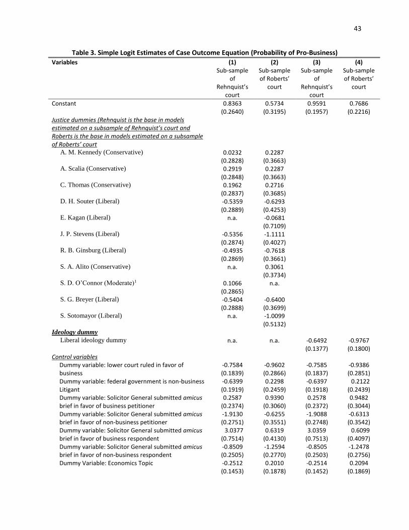
43

Table 3. Simple Logit Estimates of Case Outcome Equation (Probability of Pro-Business)

Variables (1) Sub-sample

of Rehnquist’s

court

(2) Sub-sample of Roberts’

court

(3) Sub-sample

of Rehnquist’s

court

(4) Sub-sample of Roberts’

court

Constant 0.8363 (0.2640)

0.5734 (0.3195)

0.9591 (0.1957)

0.7686 (0.2216)

Justice dummies (Rehnquist is the base in models estimated on a subsample of Rehnquist’s court and Roberts is the base in models estimated on a subsample of Roberts’ court

A. M. Kennedy (Conservative) 0.0232 (0.2828)

0.2287 (0.3663)

A. Scalia (Conservative) 0.2919 (0.2848)

0.2287 (0.3663)

C. Thomas (Conservative) 0.1962 (0.2837)

0.2716 (0.3685)

D. H. Souter (Liberal) -0.5359 (0.2889)

-0.6293 (0.4253)

E. Kagan (Liberal) n.a. -0.0681 (0.7109)

J. P. Stevens (Liberal) -0.5356 (0.2874)

-1.1111 (0.4027)

R. B. Ginsburg (Liberal) -0.4935 (0.2869)

-0.7618 (0.3661)

S. A. Alito (Conservative) n.a. 0.3061 (0.3734)

S. D. O’Connor (Moderate)1 0.1066 (0.2865)

n.a.

S. G. Breyer (Liberal) -0.5404 (0.2888)

-0.6400 (0.3699)

S. Sotomayor (Liberal) n.a. -1.0099 (0.5132)

Ideology dummy Liberal ideology dummy n.a. n.a. -0.6492

(0.1377) -0.9767 (0.1800)

Control variables Dummy variable: lower court ruled in favor of business

-0.7584 (0.1839)

-0.9602 (0.2866)

-0.7585 (0.1837)

-0.9386 (0.2851)

Dummy variable: federal government is non-business Litigant

-0.6399 (0.1919)

0.2298 (0.2459)

-0.6397 (0.1918)

0.2122 (0.2439)

Dummy variable: Solicitor General submitted amicus brief in favor of business petitioner

0.2587 (0.2374)

0.9390 (0.3060)

0.2578 (0.2372)

0.9482 (0.3044)

Dummy variable: Solicitor General submitted amicus brief in favor of non-business petitioner

-1.9130 (0.2751)

-0.6255 (0.3551)

-1.9088 (0.2748)

-0.6313 (0.3542)

Dummy variable: Solicitor General submitted amicus brief in favor of business respondent

3.0377 (0.7514)

0.6319 (0.4130)

3.0359 (0.7513)

0.6099 (0.4097)

Dummy variable: Solicitor General submitted amicus brief in favor of non-business respondent

-0.8509 (0.2505)

-1.2594 (0.2770)

-0.8505 (0.2503)

-1.2478 (0.2756)

Dummy Variable: Economics Topic -0.2512 (0.1453)

0.2010 (0.1878)

-0.2514 (0.1452)

0.2094 (0.1869)

44

Table 3. Simple Logit Estimates (continued)

(1) Sub-sample

of Rehnquist’s

court

(2) Sub-sample of Roberts’

court

(3) Sub-sample

of Rehnquist’s

court

(4) Sub-sample of Roberts’

court

Log Likelihood Number of Cases

-635.56 126

-373.84 72

-636.31 126

-375.81 72

Number of Observations ----------------------------------------------------------------------------

1115 ---------------

628 -----------------

1115 -----------------

628 -----------------

45

Table 4. Joint Estimation of Mixed-Logit Case Outcome Model and Probit Case Selection Model (The

selection model is estimated on the Bloomberg subsample) Variables (1)

Mixed logit

with control

for sample

selection on

sub-sample of

Rehnquist’s

court

(2)

Mixed logit

with control

for sample

selection on

sub-sample

of Roberts’

court

(3)

Mixed logit

with control

for sample

selection on

sub-sample

of

Rehnquist’s

court

(4)

Mixed logit

with control

for sample

selection on

sub-sample

of Roberts’

court

Part 1: Case Outcomes Equation

Constant 2.8010

(1.3275)

1.6081

(1.2006)

4.3172

(1.4235)

2.7233

(1.4282)

Justice and ideology dummies (Rehnquist as the

base in models on subsample of Rehnquist’s court

and Robert as the base in models on subsample of

Roberts’ court

A. M. Kennedy (Conservative) 0.1198

(0.5202)

0.8175

(0.7418)

A. Scalia (Conservative) 0.9548

(0.5314)

0.8175

(0.7418)

C. Thomas (Conservative) 0.6777

(0.5255)

0.9637

(0.7588)

D. H. Souter (Liberal) -0.3368

(0.8343)

-2.9337

(1.2229)

E. Kagan (Liberal) -- -3.0797

(1.5531)

J. P. Stevens (Liberal) -0.4304

(0.8355)

-3.9674

(1.2254)

R. B. Ginsburg (Liberal) -0.2859

(0.8313)

-3.1729

(1.1684)

S. A. Alito (Conservative) -- 0.8317

(0.7455)

S. D. O’Connor (Moderate)1 0.3077

(0.5271)

--

S. G. Breyer (Liberal) -0.4352

(0.8361)

-3.0045

(1.1731)

S. Sotomayor (Liberal) -- -3.0296

(1.3385)

Mean of Liberal ideology dummy -- -- -1.2839

(0.6740)

-4.7475

(1.2079)

Standard deviation of conservative/moderate

ideology dummy

6.6314

(1.0202)

8.1809

(1.5127)

6.4444

(0.9552)

7.8631

(1.9059)

Standard deviation of liberal

ideology dummy

6.8372

(1.3107)

3.8474

(0.8171)

5.1914

(0.7749)

4.0222

(0.9633)

Correlation between conservative/moderate

and liberal ideology dummy

0.6035

(0.0678)

0.4031

(0.1456)

0.5897

(0.0877)

0.6536

(0.1016)

Correlation between selection error and

conservative/moderate ideology dummy

0.7882

(0.0842)

-0.2837

(0.1012)

0.3461

(0.1263)

-0.3987

(0.1170)

Correlation between selection error and

liberal ideology dummy

0.2674

(0.1167)

0.2548

(0.2083)

0.0300

(0.1368_

0.1135

(0.1724)

46

Table 4 Joint Estimation of Mixed-Logit Case Outcome Model and Probit Case Selection Model (Continued)

Variables (1)

Mixed logit

with control

for sample

selection on

sub-sample of

Rehnquist’s

court

(2)

Mixed logit

with control

for sample

selection on

sub-sample

of Roberts’

court

(3)

Mixed logit

with control

for sample

selection on

sub-sample

of

Rehnquist’s

court

(4)

Mixed logit

with control

for sample

selection on

sub-sample

of Roberts’

court

Law variables

Dummy of lower court ruled in favor of business -4.6736

(1.3474)

-1.2649

(1.4197)

-3.4832

(1.0039)

-1.0990

(1.4430)

Dummy of federal government is non-business

litigant

-2.3399

(1.6176)

-0.5023

(1.2512)

-5.1020

(1.3870)

1.4258

(1.3066)

Dummy of Solicitor General submitted amicus

brief in favor business petitioner

-0.0743

(1.6844)

4.3603

(1.2699)

-1.0884

(1.4527)

5.4504

(1.6837)

Dummy of Solicitor General submitted amicus

brief in favor non-business petitioner

-5.4166

(1.8916)

-2.4784

(1.3156)

-9.5795

(2.1456)

-2.1486

(1.4341)

Dummy of Solicitor General submitted amicus

brief in favor business respondent

9.3134

(3.4880)

4.3911

(1.6947)

7.4362

(2.2434)

3.8868

(1.7797)

Dummy of Solicitor General submitted amicus

brief in favor non-business respondent

-4.7554

(1.8921)

-3.5744

(1.3368)

-5.4733

(1.3271)

-3.3499

(1.8787)

Dummy of Econ Topic -1.0262

(0.9549)

0.0231

(0.7125)

-0.0285

(0.7838)

0.7245

(0.8951)

Part 2: Case Selection Equation

Constant -2.1136

(0.8419)

1.7606

(1.9245)

-1.8058

(0.7576)

2.0230

(1.8823)

Lower Court Dummy 2 -0.0146

(0.2622)

0.3945

(0.3353)

0.0052

(0.2720)

0.4004

(0.3067)

Lower Court Dummy 4 0.4089

(0.2561)

-0.2276

(0.4676)

0.3910

(0.2399)

-0.2616

(0.4149)

Lower Court Dummy 6 0.4988

(0.1959)

0.2735

(0.3506)

0.4840

(0.1822)

0.2299

(0.3204)

Lower Court Dummy 7 0.0420

(0.3049)

0.4755

(0.2439)

0.1474

(0.2638)

0.4835

(0.2251)

Lower Court Dummy 8 0.4524

(0.2214)

0.5415

(0.2518)

0.5481

(0.2103)

0.5816

(0.2679)

Lower Court Dummy 9 0.3515

(0.1655)

0.2887

(0.2435)

0.3643

(0.1543)

0.3377

(0.2496)

Lower Court Dummy 11 0.2375

(0.2159)

-0.2912

(0.6416)

0.3162

(0.2078)

-0.2129

(0.6439)

Lower Court Dummy 13 0.2053

(0.3532)

0.2783

(0.4829)

0.1658

(0.3399)

0.3047

(0.4964)

Dummy of top Supreme Court advocates 1.1694

(0.1892)

0.9259

(0.2327)

1.1264

(0.1929)

1.0140

(0.2380)

Dummy of top Supreme Court advocates working

as the U.S. Solicitor General

0.5407

(0.3072)

2.1588

(0.6405)

0.5079

(0.2762)

2.0394

(0.6670)

Indicator for whether SCOTUS invited the Solicitor

General to express the views of the United States

1.0789

(0.3066)

0.9974

(0.3398)

1.0511

(0.3437)

0.9078

(0.3398)

Annual # of cases on SCOTUS docket (in

thousands)

0.0215

(0.0968)

-0.3724

(0.1732)

-0.0136

(0.0883)

-0.3599

(0.1554)

Dummy of decided in February session -0.1745

(0.2659)

-0.6020

(0.3855)

-0.2048

(0.2248)

-0.7101

(0.3469)

Dummy of decided in March session -0.0861

(0.2140)

-0.1414

(0.2858)

-0.1190

(0.2061)

-0.2298

(0.2851)

47

Table 4 Joint Estimation of Mixed-Logit Case Outcome Model and Probit Case Selection Model (Continued)

Variables (1)

Mixed logit

with control

for sample

selection on

sub-sample of

Rehnquist’s

court

(2)

Mixed logit

with control

for sample

selection on

sub-sample

of Roberts’

court

(3)

Mixed logit

with control

for sample

selection on

sub-sample

of

Rehnquist’s

court

(4)

Mixed logit

with control

for sample

selection on

sub-sample

of Roberts’

court

Dummy of decided in Summer session (Juy. – Sep.) -0.1307

(0.1581)

-0.6431

(0.2821)

-0.1937

(0.1561)

-0.6974

(0.2819)

Dummy of decided in November session -0.2137

(0.2167)

-0.6053

(0.2880)

-0.3482

(0.2036)

-0.6874

(0.2624)

Log-likelihood -650.49 -393.08 -652.79 -395.67

Number of cases in outcome equation 126 72 126 72

Number of observations in outcome equation 1115 628 1115 628

Number of cases in selection equation 1733 1035 1733 1035

Total number of observations 2848 1663 2848 1663

Note: The models are estimated by mixed-logit based on 150 halton draws.

Table 5. Comparing the Predicted Probability of Voting Pro-Business across Models

(1)

Simple logit

without control

for case selection

on full sample of

justices (Model 3

and 4 of Table 3)

(2)

Simple logit

without control

for case

selection on

subsample of

justices serving

both courts

(3)

Mixed logit with

control for case

selection on full

sample of justices

(Model 3 and 4 of

Table 5

(4)

Mixed logit with

control for case

selection on

subsample of

justices serving both

courts (Model 1 and

2 of Table 7)

Rehnquist court

Conservative justices

(p1)

Liberal justices (p2)

Probability of p1 > p2

0.50

0.37

0.99

0.51

0.37

0.99

0.44

0.36

0.96

0.45

0.39

0.95

Roberts court

Conservative justices

(p1)

Liberal justices (p2)

Probability of p1 > p2

0.61

0.40

0.99

0.61

0.40

0.99

0.65

0.38

0.99

0.65

0.37

0.99

48

Appendix Table 1. Estimation Results of Petition Selection Model (Probability of Being Approved)

Parameters in Selection Model (1)

Simple Probit

on Bloomberg

subsample

during the

period of

Rehnquist’s

court

(2)

Simple Probit

on Bloomberg

subsample

during the

period of

Roberts’ court

(3)

WESMLE on

subsample of

Rehnquist’s court

(including both

Bloomberg

subsample and

BLD subsample)

(4)

WESMLE on

subsample of

Roberts’ court

(including both

Bloomberg

subsample and

BLD subsample)

Constant -2.0380

(0.8624)

1.9961

(1.8010)

-1.5856

(0.9389)

0.7962

(1.9629)

Lower Court Dummy 1 -- -- 0.3860

(0.4233)

0.1861

(0.6968)

Lower Court Dummy 2 0.0042

(0.2899)

0.2906

(0.2892)

0.1861

(0.3071)

0.7287

(0.3210)

Lower Court Dummy 3 0.0589

(0.3502)

0.2124

(0.3838)

0.2476

(0.3650)

0.3580

(0.4612)

Lower Court Dummy 4 0.3412

(0.2553)

-0.3121

(0.4654)

0.4014

(0.2937)

0.0418

(0.4897)

Lower Court Dummy 5 0.2715

(0.2196)

-0.3221

(0.4321)

0.2819

(0.2560)

-0.3628

(0.6132)

Lower Court Dummy 6 0.5793

(0.2293)

0.2528

(0.3010)

0.4978

(0.2444)

0.4817

(0.3598)

Lower Court Dummy 7 0.0597

(0.3056)

0.5218

(0.2909)

0.3867

(0.2972)

0.7409

(0.3513)

Lower Court Dummy 8 0.4994

(0.2558)

0.5272

(0.3616)

0.5918

(0.2725)

0.6114

(0.4646)

Lower Court Dummy 9 0.4081

(0.1895)

0.2382

(0.2449)

0.6289

(0.2077)

0.5711

(0.2809)

Lower Court Dummy 10 -0.2829

(0.4503)

0.0883

(0.4714)

-0.0332

(0.4262)

0.3619

(0.5042)

Lower Court Dummy 11 0.3473

(0.2268)

-0.2875

(0.4190)

0.3232

(0.2690)

0.4035

(0.3657)

Lower Court Dummy 12 -0.3702

(0.5802)

-0.2065

(0.4783)

0.4917

(0.3740)

0.1795

(0.4836)

Lower Court Dummy 13 0.2502

(0.4372)

0.2808

(0.4400)

0.2628

(0.4801)

0.5228

(0.5037)

Dummy of top Supreme Court

advocates

1.1768

(0.2355)

0.9854

(0.2400)

1.3549

(0.2451)

1.4328

(0.2369)

Dummy of top Supreme Court

advocates working as the U.S.

Solicitor General

0.9679

(0.4344)

1.8329

(0.6873)

0.9089

(0.4503)

1.1075

(0.5289)

Indicator for whether SCOTUS invited

the Solicitor General to express the

views of the United States

1.1705

(0.4505)

0.6446

(0.4157)

1.7903

(0.4029)

1.1734

(0.4086)

Annual # of cases on SCOTUS docket

(in thousands)

0.0163

(0.0970)

-0.3666

(0.1909)

-0.0543

(0.1043)

-0.2624

(0.1480)

Dummy of decided in January session -0.0468

(0.2693)

-0.2972

(0.3070)

0.3107

(0.3230)

-0.2519

(0.3729)

Dummy of decided in February

session

-0.2784

(0.3094)

-0.9296

(0.4790)

-0.1365

(0.3772)

-0.7504

(0.5272)

Dummy of decided in March session -0.1995

(0.2923)

-0.4396

(0.3637)

-0.0669

(0.3628)

-0.3920

(0.4460)

Dummy of decided in April session -0.0537 -0.4401 0.0959 -0.2593

49

(0.2835) (0.3781) (0.3531) (0.4411)

Appendix Table 1. Estimation Results of Petition Selection Model (Continued) Parameters in Selection Model (1)

Simple Probit

on Bloomberg

subsample

during the

period of

Rehnquist’s

court

(2)

Simple Probit

on Bloomberg

subsample

during the

period of

Roberts’ court

(3)

WESMLE on

subsample of

Rehnquist’s court

(including both

Bloomberg

subsample and

BLD subsample)

(4)

WESMLE on

subsample of

Roberts’ court

(including both

Bloomberg

subsample and

BLD subsample)

Dummy of decided in May session -0.4285

(0.3340)

-0.7354

(0.3877)

0.1212

(0.3548)

-0.5188

(0.2428)

Dummy of decided in June session -0.3033

(0.2819)

-0.1516

(0.3010)

-0.0216

(0.3388)

0.0554

(0.3627)

Dummy of decided in Summer session -0.2496

(0.2574)

-0.9356

(0.3209)

-0.0849

(0.3220)

-0.6086

(0.2613)

Dummy of decided in October session 0.1596

(0.2857)

-0.2477

(0.3389)

0.3079

(0.3574)

-0.2131

(0.4193)

Dummy of decided in November

session

-0.2204

(0.3007)

-0.8923

(0.3985)

0.1559

(0.3481)

-0.4479

(0.4096)

Log-likelihood -260.67 -158.62 -228.01 -130.64

Number of observations 1697 1017 1865 1107

50

Appendix Table 2. Robustness Checks: Joint Estimation of Mixed-Logit Case Outcome Model and Probit

Case Selection Model (The selection model is estimated on combined sample of Bloomberg and BLD by

WESMLE) Variables (1)

Mixed logit

with control

for sample

selection on

sub-sample of

Rehnquist’s

court

(2)

Mixed logit

with control

for sample

selection on

sub-sample of

Roberts’

court

Constant 5.5695

(1.1404)

3.3165

(1.4895)

Mean of Liberal ideology dummy -1.7092

(0.8784)

-5.6606

(1.2241)

Standard deviation of conservative/moderate ideology dummy 6.3281

(0.8660)

7.0422

(1.4031)

Standard deviation of liberal ideology dummy 4.9800

(0.7679)

4.5366

(0.9313)

Correlation between conservative/moderate and liberal ideology dummy 0.5851

(0.0538)

0.5922

(0.1091)

Correlation between selection error and conservative/moderate ideology dummy -0.0078

(0.1190)

-0.3002

(0.0999)

Correlation between selection error and liberal ideology dummy 0.0391

(0.1161)

0.2378

(0.1258)

Dummy of lower court ruled in favor of business -3.3560

(0.9192)

-1.9499

(1.4776)

Dummy of federal government is non-business litigant -3.8810

(0.9272)

1.3408

(1.1422)

Dummy of Solicitor General submitted amicus brief in favor business petitioner -1.1567

(1.1418)

5.3745

(1.7223)

Dummy of Solicitor General submitted amicus brief in favor non-business petitioner -7.5675

(1.3817)

-2.5675

(1.2744)

Dummy of Solicitor General submitted amicus brief in favor business respondent 6.2962

(2.0716)

2.1809

(1.4600)

Dummy of Solicitor General submitted amicus brief in favor non-business respondent -4.6294

(1.2893)

-4.0472

(1.8942)

Dummy of Econ Topic -2.4573

(0.7757)

1.5659

(0.9809)

Note: The models are estimated by mixed-logit based on 150 halton draws.

51

Appendix Table 3. Robustness Checks: Joint Estimation of Mixed-Logit Case Outcome Model and Probit

Case Selection Model on the Subsample of Justices Serving Both the Two Courts (The selection model is

estimated on Bloomberg subsample) Variables (1)

Mixed logit

with control

for sample

selection on

sub-sample of

Rehnquist’s

court

(2)

Mixed logit

with control

for sample

selection on

sub-sample of

Roberts’

court

Constant 3.3177

(1.3065)

2.3634

(1.4885)

Mean of Liberal ideology dummy -0.8635

(0.7036)

-4.1260

(1.4507)

Standard deviation of conservative/moderate ideology dummy 7.0545

(1.2603)

5.8860

(1.3727)

Standard deviation of liberal ideology dummy 4.8685

(0.8248)

3.6559

(0.9833)

Correlation between conservative/moderate and liberal ideology dummy 0.6393

(0.0951)

0.6007

(0.1459)

Correlation between selection error and conservative/moderate ideology dummy 0.1607

(0.1540)

-0.4614

(0.1625)

Correlation between selection error and liberal ideology dummy -0.3987

(0.1744)

0.1563

(0.2582)

Dummy of lower court ruled in favor of business -1.1666

(1.0046)

-1.2962

(1.4809)

Dummy of federal government is non-business litigant -3.4255

(1.3501)

0.8048

(1.4770)

Dummy of Solicitor General submitted amicus brief in favor business petitioner 0.4107

(1.4728)

3.9246

(1.3854)

Dummy of Solicitor General submitted amicus brief in favor non-business petitioner -8.8758

(2.7223)

-2.3508

(2.3761)

Dummy of Solicitor General submitted amicus brief in favor business respondent 4.9079

(2.8453)

2.3607

(2.0504)

Dummy of Solicitor General submitted amicus brief in favor non-business respondent -6.1006

(1.7604)

-2.6100

(1.5831)

Dummy of Econ Topic -1.1574

(0.8247)

1.0085

(0.9848)

Note: The models are estimated by mixed-logit based on 150 halton draws. Justices included in the estimations are:

A. M. Kennedy, A. Scalia, C. Thomas, D. H. Souter, J. P. Stevens, R. B. Ginsburg and S. G. Breyer.

52

Appendix Table 4. Robustness Checks of adding case topic and lower court fixed effects: Joint

Estimation of Mixed-Logit Case Outcome Model and Probit Case Selection Model (The selection model is

estimated on Bloomberg subsample) Variables (1)

Mixed logit

with control

for sample

selection on

sub-sample of

Rehnquist’s

court

(2)

Mixed logit

with control

for sample

selection on

sub-sample of

Roberts’

court

Constant 4.4045

(2.7764)

2.8191

(2.1400)

Mean of Liberal ideology dummy -1.0040

(0.6013)

-5.1686

(1.2534)

Standard deviation of conservative/moderate ideology dummy 8.6551

(1.6164)

9.5883

(2.1310)

Standard deviation of liberal ideology dummy 5.9190

(0.9341)

2.3038

(0.6250)

Correlation between conservative/moderate and liberal ideology dummy 0.7825

(0.0435)

0.8140

(0.1277)

Correlation between selection error and conservative/moderate ideology dummy 0.0448

(0.0617)

-0.4142

(0.1188)

Correlation between selection error and liberal ideology dummy -0.0587

(0.0832)

0.1221

(0.2710)

Dummy of lower court ruled in favor of business -2.1376

(0.9353)

-2.0276

(1.4885)

Dummy of federal government is non-business litigant -6.6409

(1.4342)

-0.2087

(1.2293)

Dummy of Solicitor General submitted amicus brief in favor business petitioner -0.3641

(1.0878)

5.4587

(1.3216)

Dummy of Solicitor General submitted amicus brief in favor non-business petitioner -10.5239

(1.9762)

0.3378

(1.7038)

Dummy of Solicitor General submitted amicus brief in favor business respondent 5.8586

(2.4971)

7.1721

(2.5242)

Dummy of Solicitor General submitted amicus brief in favor non-business respondent -8.0782

(1.6168)

-0.8091

(1.4355)

Dummy of Econ Topic -3.2435

(0.9212)

0.1611

(0.9433)

Case topic dummies included? YES YES

Lower court dummies included? YES YES