Suppression of Arctic Air Formation with Climate Warming ... · PDF fileSuppression of Arctic...

Suppression of Arctic Air Formation with Climate Warming:Investigation with a Two-Dimensional Cloud-Resolving Model

TIMOTHY W. CRONIN

Department of Earth, Atmospheric, and Planetary Sciences, Massachusetts Institute of Technology,

Cambridge, Massachusetts

HARRISON LI

Harvard University, Cambridge, Massachusetts

ELI TZIPERMAN

Department of Earth and Planetary Sciences, and School of Engineering and Applied Sciences,

Harvard University, Cambridge, Massachusetts

(Manuscript received 23 June 2016, in final form 2 June 2017)

ABSTRACT

Arctic climate change inwinter is tightly linked to changes in the strength of surface temperature inversions,

which occur frequently in the present climate as Arctic air masses form during polar night. Recent work

proposed that, in a warmer climate, increasing low-cloud optical thickness of maritime air advected over high-

latitude landmasses during polar night could suppress the formation of Arctic air masses, amplifying winter

warming over continents and sea ice. But this mechanism was based on single-column simulations that could

not assess the role of fractional cloud cover change. This paper presents two-dimensional cloud-resolving

model simulations that support the single-column model results: low-cloud optical thickness and duration

increase strongly with initial air temperature, slowing the surface cooling rate as the climate is warmed. The

cloud-resolving model cools less at the surface than the single-columnmodel, and the sensitivity of its cooling

to warmer initial temperatures is also higher, because it produces cloudier atmospheres with stronger lower-

tropospheric mixing and distributes cloud-top cooling over a deeper atmospheric layer with larger heat ca-

pacity. Resolving larger-scale cloud turbulence has the greatest impact on the microphysics schemes that best

represent general observed features of mixed-phase clouds, increasing their sensitivity to climate warming.

These findings support the hypothesis that increasing insulation of the high-latitude land surface by low clouds

in a warmer world could act as a strong positive feedback in future climate change and suggest studyingArctic

air formation in a three-dimensional climate model.

1. Introduction

In recent decades, the Arctic has warmed faster than

the rest of the globe, particularly during winter (Chylek

et al. 2009; Hartmann et al. 2013), and Arctic-amplified

warming is expected to continue through the twenty-first

century according to climate model simulations

(Holland and Bitz 2003; Pithan and Mauritsen 2014).

Arctic amplification of temperature change occurs in

models primarily because of positive feedbacks that act

at high latitudes, especially those related to decreased

surface albedo from melting of ice and snow, and to

changes in the tropospheric lapse rate (Pithan and

Mauritsen 2014), though it can also occur without locally

amplifying feedbacks because of increased poleward

atmospheric heat transport (e.g., Alexeev and Jackson

2013). Although changes in tropospheric lapse rate

contribute strongly to Arctic amplification, assessment

of lapse-rate changes in models has often been di-

agnostic; a more process-based understanding of the

controls on high-latitude lapse rates and surface in-

version strength is needed.

Supplemental information related to this paper is available at

the Journals Online website: http://dx.doi.org/10.1175/JAS-D-16-

0193.s1.

Corresponding author: Timothy W. Cronin, [email protected]

SEPTEMBER 2017 CRON IN ET AL . 2717

DOI: 10.1175/JAS-D-16-0193.1

� 2017 American Meteorological Society. For information regarding reuse of this content and general copyright information, consult the AMS CopyrightPolicy (www.ametsoc.org/PUBSReuseLicenses).

http://dx.doi.org/10.1175/JAS-D-16-0193.s1

http://dx.doi.org/10.1175/JAS-D-16-0193.s1

mailto:[email protected]

http://www.ametsoc.org/PUBSReuseLicenses



Recent work by Cronin and Tziperman (2015) found

amplified surface warming and weaker surface inversions

over high-latitude winter continents due to increasing

insulation of the surface by optically thick liquid clouds

in a single-column model. The goal of this study is to test

the viability and strength of this mechanism—increased

surface insulation by low clouds in a warmer world—in

a model that resolves cloud dynamics at scales of

;100 m–10 km and to compare cloud-resolving and

single-column model results.

Arctic air formation is an initial-value problem in

which an air mass with a prescribed initial temperature

and moisture profile is allowed to cool by radiation to

space over a low-heat-capacity surface in the absence of

sunlight. This idealized problem represents the advec-

tion of maritime air over high-latitude land or sea ice

during polar night. The concept of Arctic air formation

was first introduced byWexler (1936), who explored the

transformation of polar maritime air into Arctic air by

longwave radiative cooling in the absence of sunlight or

clouds. Based on observed soundings during events of

high-latitude airmass stagnation over land, Wexler

(1936) suggested that the temperature profile of an

Arctic air mass could be represented by a relatively cold

isothermal layer overlying an even colder surface in-

version layer. Both the isothermal layer and the in-

version layer cool as time progresses and the isothermal

layer deepens; in essence, radiative cooling of the sur-

face to space steadily consumes the heat content of the

lower troposphere from beneath.

Work since the study ofWexler (1936) has slowly built

fromhis original idea. Curry (1983) used a one-dimensional

model with more detailed radiative transfer to examine

the role of clouds, subsidence, and turbulence on the

formation of Arctic air and found that the process is

especially sensitive to the amount of condensate in the

atmosphere and its partitioning between liquid and ice.

Overland and Guest (1991) conducted longer simula-

tions, including a modification of the problem to explore

equilibrium Arctic atmospheric temperature structure

in winter. They also examined the rapid adjustment of

surface temperature and inversion strength to transi-

tions between clear and cloudy skies. Emanuel (2008)

performed single-column model calculations of Arctic

airmass formation and showed that, owing to its large

static stability, Arctic air has greater saturation potential

vorticity relative to the rest of the troposphere, which

may allow it to play an important role in development of

midlatitude weather systems.

Arctic air formation has also been linked to the

broader investigation of Arctic mixed-phase clouds and

boundary layer dynamics, airmass transformation, and

the role of the surface energy balance throughout the

year in sea ice loss. The longwave radiative effect of

clouds is a large term in the Arctic surface energy bal-

ance in all seasons and consequently regulates ice loss

over both land and sea, with more ice loss typical under

cloudy conditions despite less absorption of shortwave

radiation (Kapsch et al. 2013; Van Tricht et al. 2016;

Mortin et al. 2016). From a Lagrangian standpoint,

clouds form as warm and moist air masses are advected

and cooled over the Arctic Ocean in both summer,

leading to ice melt and fog (Tjernstrom et al. 2015), and

winter, leading to bottom-heavy warming and weaken-

ing of surface inversions (Woods and Caballero 2016).

A key finding from recent field studies in the Arctic is

bimodality of the Arctic winter boundary layer: the

coupled system of boundary layer and surface prefer to

reside in either a ‘‘radiatively clear’’ state or an

‘‘opaquely cloudy’’ state (Stramler et al. 2011; Morrison

et al. 2012). The radiatively clear state is characterized

by clear skies or optically thin ice cloud, a colder surface

and stronger surface inversion, and net surface radiative

cooling of ;40Wm22, whereas the opaquely cloudy

state is characterized by presence of cloud liquid, a

warmer surface under a weaker elevated inversion, and

near-zero surface net radiation. Pithan et al. (2014)

found that similar distinct clear and cloudy states emerge

in a single-column simulation ofArctic air formation and

that a bimodal distribution of surface longwave radiation

emerges when the transient cooling process is sampled in

time. They also found that many climate models fail to

capture this bimodality because of insufficient mainte-

nance of supercooled cloud liquid and thus a poor rep-

resentation of Arctic mixed-phase clouds. Pithan et al.

(2016) followed on this work and used an in-

tercomparison of Arctic air formation in single-column

versions of several weather and climate models to un-

derstand the strengths and biases in model representa-

tion of both the clear and cloudy boundary layer states.

Cronin and Tziperman (2015) focused on the climate

sensitivity of the process of Arctic air formation, by

modifying the temperature of the initial sounding (rep-

resenting maritime air) while holding relative humidity

fixed. They found that a warmer initial atmosphere leads

to longer-lasting low clouds and a reduced surface

cooling rate, suppressing Arctic air formation and po-

tentially amplifying winter continental warming, which

would help explain continental warmth in past climates

(e.g., Greenwood and Wing 1995). Increasing optical

thickness of low clouds with warming results from both

increasing condensate amount and from the change in

cloud phase from ice to liquid. From the perspective of

boundary layer states, a warmer initial atmosphere in-

creases the fraction of the cooling period spent in the

opaquely cloudy state.

2718 JOURNAL OF THE ATMOSPHER IC SC IENCES VOLUME 74

One potential concern that could be raised with these

findings, however, is that the single-column model used

in Cronin and Tziperman (2015) did not allow for frac-

tional cloud cover. A decrease in cloud fraction with

warming would damp the effect of more cloud conden-

sate on reducing the surface cooling rate. Furthermore,

all single-column models rely on parameterizations to

represent processes of convection, cloud-top mixing,

and entrainment, which are important in Arctic mixed-

phase clouds and may change with warming (e.g.,

Morrison et al. 2012). It is not trivial that a two-

dimensional model, which explicitly resolves these

processes down to a scale of a few hundred meters (al-

though parameterizations are still used for mixing at

smaller scales), would have the same sensitivity to

warming as a single-column model.

To test the suppression of Arctic air formation with

climate warming found by Cronin and Tziperman

(2015), this paper studies the process of Arctic air for-

mation and its sensitivity to temperature in a two-

dimensional cloud-resolving model. We find that

clouds tend to have large fractional area coverage and

that increased mixing and deeper cloud layers actually

lead to more cloud cover and less surface cooling in the

two-dimensional model than in the single-column

model. Thus, sensitivity of the two-dimensional model

is broadly consistent with Cronin and Tziperman (2015):

warming of the initial atmosphere leads to more low

clouds and a reduced surface cooling rate. The two-

dimensional model, however, is even more sensitive

than the single-column model to warming of the initial

atmosphere, especially for the microphysics schemes

with the best representation of general observed fea-

tures found in mixed-phase clouds. We describe the

model setup in section 2, present results in section 3, and

discuss our findings in section 4.

2. Model description

We use a two-dimensional idealized configuration

of the Weather Research and Forecasting (WRF, ver-

sion 3.4.1) Model to simulate the process of Arctic air

formation over a low–heat-capacity land surface for a

14-day period during polar night. Simulations span a

range of different initial temperature profiles and mi-

crophysics schemes. Many aspects of the model setup

follow Cronin and Tziperman (2015), and these are

summarized below. The surface is a uniform moist slab

with the roughness of an ocean surface and heat capacity

CS 5 2.1 3 105 Jm22K21. This heat capacity is equiva-

lent to a water layer of depth of 5 cm and corresponds to

the heat capacity of the surface layer of a deep snowpack

that communicates with the atmosphere on a 1-day time

scale. Roughness lengths in the main set of simulations

are ;1–4 3 1025m; sensitivity tests with larger rough-

ness lengths of 1024 and 1023m differ little in a quali-

tative sense but have slightly colder 2-m air

temperatures because the cold surface is more strongly

coupled to the atmosphere. Initial temperature profiles

are defined by a single parameter, the initial 2-m air

temperature T2(0) (note that we use the terms ‘‘2-m air

temperature’’ and ‘‘surface air temperature’’ in-

terchangeably in this paper). Above the surface, initial

soundings have a tropospheric lapse rate that is either

moist adiabatic or28Kkm21, whichever is more stable,

and an isothermal stratosphere at 2608C. The initial

relative humidity profile decreases from 80% at the

surface to 20% at 600hPa; above 600hPa the relative

humidity is constant at 20%up to the tropopause and set

to a mixing ratio of 0.003 gkg21 in the stratosphere.

These temperature and humidity profiles are chosen to

mimic those in Pithan et al. (2014) and Pithan et al.

(2016), but with moist adiabatic stratification allowing

for extension to warmer initial profiles without leading

to moist convective instability. In this paper, we use the

phrase ‘‘climate warming’’ synonymously with ‘‘warm-

ing of the initial atmospheric state.’’

The model domain is 15 km long, ;15km high, and

periodic in the horizontal, with a horizontal grid spacing

of 100m and a uniform initial vertical grid spacing of

50m. Cronin and Tziperman (2015) used a stretched

grid, with spacing increasing from ;20m at the surface

to ;200m at 2-km altitude and becoming even coarser

higher up, so this study represents all clouds that are not

fog with more vertical detail. The model time step for

dynamics is 1.5 s, the Coriolis parameter is set to zero,

and no cumulus parameterization scheme is used. The

spacing of levels in height decreases with time in each

simulation because the vertical coordinate in the model

is based on hydrostatic pressure, so cooling causes

compression (by roughly 20% for 558C of cooling at a

starting temperature of 08C). Although the simulations

in Cronin and Tziperman (2015) extend to 35-km height,

we reduce the vertical extent of the model here because

the stratosphere is not essential for this problem. We

also run the model with varied grid spacing in both the

horizontal and vertical to test the robustness of the main

results (see section 4d). To stimulate turbulent mixing

near the surface (both parameterized mixing and re-

solved eddies) and prevent the development of sta-

tionary surface temperature heterogeneities, a uniform

initial 5m s21 zonal wind is imposed everywhere, and

the horizontal-mean flow is relaxed to this value over a

1-day period. To allow development of horizontal

asymmetries, we initialize the lowest four levels in the

model with random temperature perturbations that are


spatially white and chosen from a uniform distribution

between 20.1 and 10.1K.

Longwave radiative transfer in the model is parame-

terized using the Rapid Radiative Transfer Model for

GCMs (RRTMG) scheme (Iacono et al. 2008), which is

called every 2min. Sensitivity tests with 6 s between ra-

diation calls lead to minimal difference in the results but

are substantially more computationally costly. Short-

wave radiation is zero at all times, because the latitude is

set to 908N, and the model runs occur during the first

2 weeks of January. We use the Yonsei University

(YSU) boundary layer scheme, which diffuses heat and

moisture nonlocally within a layer of depth diagnosed

using a bulk Richardson number (Hong et al. 2006).

Because the near-surface stability in our model setup is

often very high, and winds are relatively weak, di-

agnosed boundary layer depths are small: rarely up to a

few hundred meters and often less than 50m in depth.

Resolved turbulent flow dominates transport above this

height. Surface turbulent fluxes are parameterized using

Monin–Obukhov similarity with separate lookup func-

tions for different stability classes, and the latent heat

flux is not allowed to be negative (i.e., there is no dew or

frost). Test simulations allowing for dew and frost show

small effects on the surface energy balance and do not

substantially alter our findings.

One advantage of using WRF is the ability to easily

test different parameterizations of cloud microphysics.

The six schemes are denoted Lin–Purdue, WRF single-

moment 6-class (WSM6), Goddard, Thompson, Morrison,

and Stony Brook, and some basic information on each is

given in the appendix, with a focus on generation pro-

cesses for cloud ice. Microphysics schemes are called at

every model time step. As in Cronin and Tziperman

(2015), some results are shown only for the Lin–Purdue

microphysics scheme, but many plots show the mean

and spread of the six microphysics schemes used. The

Lin–Purdue scheme is a relatively simple bulk (single

moment) scheme that models six hydrometeors—water

vapor, cloud liquid, cloud ice, snow, rain, and graupel—

assuming exponential size distributions of rain, snow,

and graupel particles (Lin et al. 1983). We also perform

sensitivity tests labeled ‘‘no-CRF,’’ where cloud–

radiation interactions are disabled; the Lin–Purdue

scheme is still used, but cloud water concentrations are

set to zero in the radiative transfer scheme (latent heat

associated with phase changes is still considered).

Comparing no-CRF results to the results with radia-

tively active clouds allows us to quantify the impact of

cloud longwave forcing on Arctic air formation.

To explore the effects of surface heterogeneity, we

also perform a set of sensitivity tests with the Lin–

Purdue scheme, where the surface heat capacity is

heterogeneous but has the same domain-average value.

We set CS 5 9.66 3 105 Jm22K21 (23 cm of water

equivalent) in a contiguous 10%of the domain andCS51.26 3 105 Jm22K21 (3 cm of water equivalent) else-

where. This heterogeneity in surface heat capacity is

intended as a crude representation of leads in sea ice, or

areas of shallow water over land (i.e., lakes, wetlands,

and streams). Although the true heat capacity of such

heterogeneities in land cover would likely be larger, we

do not want to complicate the interpretation of these

sensitivity tests by also modifying the domain-average

surface heat capacity. Limitations in our treatment of

the surface are further discussed in section 4d.

One important caveat of this modeling setup is that,

although some of the microphysics schemes predict

particle sizes in different categories, this information is

not passed to the RRTMG radiation scheme. Rather, in

the version of WRF that we use, only the total cloud

liquid and ice content in each column and vertical level

is passed to RRTMG, and the radiation scheme makes

assumptions about the cloud particle sizes. With more

complete radiation–microphysics coupling, differences

in microphysics schemes would likely affect the results

more than indicated here.

3. Results

a. Time evolution of temperature and clouds

An increase in cloudiness with warmer initial states is

evident from snapshots of modeled Arctic air formation

after 4 days of cooling from initial 2-m air temperatures

T2(0) of 08, 108, and 208C and the Lin–Purdue micro-

physics scheme (Fig. 1). Video S1 in the supplemental

material also shows the evolution of the cloud fields and

temperature profiles over the whole 2-week period;

below, we summarize this evolution over the first 4 days

to explain the origins of different cloud structures in

Fig. 1. Analogous supplemental videos S2–S6 are in-

cluded to show simulations with the other microphysics

schemes but are not discussed in detail.

When the initial surface temperature is T2(0)5 08C(Fig. 1a), a physically thin but optically thick mixed-

phase fog forms after about 6 h of initial clear-sky

cooling but dissipates in roughly a day as a result of

scavenging of cloud water by snow, leaving behind ten-

uous ice clouds and snow. Although the surface tem-

perature rebounds slightly when fog forms, the first

4 days are dominated by clear-sky surface cooling by

more than 258C and development of a strong surface

inversion. With a warmer initial surface temperature of

T2(0)5 108C (Fig. 1b), a surface fog layer again forms

after about 6 h, but it is all liquid and deepens rapidly.

An elevated stratus layer detaches from the surface fog


around hour 36, grows upward into the clear background

air, develops some ice after about hour 48 as it continues

to cool, and then dissipates rapidly by precipitation just

before the end of day 3. A new cloud layer beneath,

limited in its growth by effects of the overlying cloud

layer (weakened radiative cooling and precipitation),

then rapidly thickens and deepens and repeats the cycle

of growth and decay over day 4. At the end of day 4, the

broken remnants of this second mixed-phase stratus

cloud layer lie at about 1.5-km altitude, and a new liquid

fog layer is beginning to form at the surface. As a con-

sequence of strong longwave cloud radiative forcing

during this sequence of two cloud-layer life cycles, the

surface has cooled only by about 128C by the end of the

fourth day, and there is only a very weak surface in-

version. For an even warmer initial surface temperature

of T2(0)5 208C (Fig. 1c), the initial evolution and

growth of the surface fog layer is very similar to the

T2(0)5 108C case. The stratus layer at ;2.5 km, how-

ever, has persisted continuously since it detached from

the initial fog layer around hour 32 and is only just be-

ginning to develop ice and dissipate in the snapshot

shown in Fig. 1c. There is also a second optically thick

liquid cloud layer below it. This abundant and persistent

cloud cover displaces radiative cooling upward from the

surface to the top of the upper cloud layer, resulting in

only ;108C of surface cooling by the end of the fourth

day, with the low-level lapse rate remaining nearly moist

adiabatic as in the initial state. At the end of day 4, the

region between the two cloud layers for T2(0)5 208C is

convective (see video S1), with horizontal fluctuations of

vertical velocity ;0.2m s21.

The behavior and structure of mixed-phase clouds in

the warm and very warm simulations [T2(0) 5 108 and208C, respectively] in Fig. 1 bear some resemblance to

real Arctic mixed-phase clouds. Supercooled liquid

overlies ice, ice and snow fall gradually, updrafts and

entrainment through amoist inversion supply new cloud

water, and multiple cloud layers form in areas of both

stable and moist adiabatic stratification (e.g., Morrison

et al. 2012; Sedlar et al. 2011; Verlinde et al. 2013). The

most serious deficiencies of the simulations with the

Lin–Purdue scheme are that new clouds are too com-

monly mixtures of ice and liquid because of the im-

plementation of supersaturation adjustment (see the

appendix) and that the scheme does not maintain

enough supercooled liquid at low temperatures. In-

spection of theWRF implementation of the Lin–Purdue

scheme reveals that it cannot form any new supercooled

liquid by condensation below 2258C and thus cannot

simulate persistent mixed-phase clouds when the cloud

layer cools below 2108C, instead switching rapidly into

the radiatively clear boundary layer state. Other

schemes generally share this deficiency of maintaining

too little supercooled liquid—or, equivalently, a too-

high glaciation temperature (see the appendix)—similar

to findings by Pithan et al. (2014) for global models. In

broad terms, the WSM6 (video S2) and Goddard (video

S3) schemes do a poorer job than the Lin–Purdue

scheme of representing mixed-phase clouds; they both

FIG. 1. Snapshots at day 4 of clouds as a function of height and x coordinate for simulations with initial 2-m temperatures of (a) 08,(b) 108, and (c) 208C. Cloud liquid and cloud ice content are plottedwith a two-dimensional logarithmic scale inset in (a): light to dark blues

indicate cloud ice from 0.001 to 0.1 g kg21, light to dark greens indicate cloud liquid from 0.01 to 1 g kg21, and shades of cyan indicate

mixed-phase clouds containing both liquid and ice. (d) Domain-average temperature profiles show development of a strong surface-based

inversion in the cold simulation and deeper but less-cold convective surface layers beneath cloud-top inversions for the warmer simu-

lations. Video S1 shows time evolution of this figure over the full 14 days of the three simulations.


lack the basic supercooled liquid-over-ice morphology.

WSM6 simulates much more cloud ice than any other

scheme and has a glaciation temperature only slightly

below 08C. The Thompson (video S4) and Morrison

(video S5) schemes represent mixed-phase clouds better

than the Lin–Purdue scheme: both are able tomaintain a

mixed-phase cloud layer that grows upward and persists

for 2–3 days in the T2(0)5 08C case. Morrison and Pinto

(2005), one of the primary papers documenting the

Morrison scheme, applied it in WRF to a case study of

Arctic mixed-phase stratus and found that the scheme

was able to capture key qualitative features of the

clouds, as well as quantitative features such as cloud

droplet number concentration and cloud water path.

The Stony Brook (video S6) scheme has nearly identical

cloud ice and cloud liquid physics to the Lin scheme and

thus has similar strengths and weaknesses in depicting

Arctic mixed-phase clouds.

Snapshots of domain-average soundings and cloud

properties every 2 days during the cooling process also

show the strong increase in cloudiness with warming of

the initial state for the Lin–Purdue microphysics scheme

(Fig. 2). Whenever low-level liquid clouds are present,

they prevent the development of the surface inversion

characteristic of Arctic air, instead giving rise to a strong

cloud-top inversion with temperatures increasing from

the cloud top down to the surface (Fig. 2). Consequently,

the simulation with T2(0)5 208C has a total surface air

temperature decrease of 39.78C over 2 weeks, compared

to 52.28C for T2(0)5 108C and 57.38C for T2(0)5 08C.Comparing the evolution of surface longwave fluxes

(Fig. 3a) with the soundings in Fig. 2 shows the corre-

spondence between suppressed surface cooling rates

and the presence of low-level liquid clouds. Figure 3c

explicitly shows that warmer initial states have a more

positive and more persistent surface cloud longwave

forcing; for the warmest case, surface cloud longwave

forcing increases until after day 10. Turbulent surface

heat fluxes also regulate the total cooling rate under

clear skies; once the cloud layer dissipates in each sim-

ulation, about half of the surface radiative cooling is

offset by sensible heating of the surface (by warmer

overlying air in the surface inversion; negative fluxes

indicate warming of the surface in Fig. 3b).

Synchronous spikes in surface longwave cooling (up-

ward) and surface cloud radiative effect and condensate

path (downward) appear prominently for the warmest

simulation in Fig. 3. These spikes occur as a result of

quasi-periodic formation and upward propagation of a

near-surface fog and stratus cloud layer, which re-

peatedly transforms into cumulus convection and dissi-

pates, allowing the surface to cool and again form a fog

layer (see video S1; frames near and leading up to a

spike at day 4, hour 21 provide a good example). The

frequency of these spikes is ;1–2 day21, but the timing,

regularity, and amplitude varies substantially across

microphysics schemes (see videos S2–S6). Although

these spikes are an intriguing feature of the warmer

simulations, they do not seem to play a key role in any of

the main conclusions, and, consequently, we do not

discuss them further.

Simulations with heterogeneous surface heat capacity

share many of these features, with similar time series of

surface energy balance, cloud radiative forcing, vertically

integrated cloud condensate, and even similar timing of

spikes in the warmest simulation (dashed-dotted lines in

Fig. 3). An additional result from these simulations is that

thick clouds not only suppress surface cooling, they also

reduce the spatial variability in surface air temperature

(Fig. 3e). In clear-sky conditions, the surface cools less

quickly where it has high heat capacity, and more quickly

elsewhere. This differential surface cooling rate leads to

2-m air temperatures that vary spatially by ;48C in the

clear state, but only;0.58C in the cloudy state. Increased

duration of optically thick clouds in a warmer initial at-

mosphere thus allows not only for maintenance of

warmer conditions overall, but also for better re-

distribution of heat within the domain, from locally warm

areas to locally cold ones. A speculative consequence of

this finding would be that inland water bodies—even if

they are relatively shallow—could play more of a role in

moderating continental temperatures in warmer climates

because their heat could be redistributed nonlocally by

advection in a deeper cloud-topped boundary layer,

rather than being lost locally by radiation to space.

Surface air temperature evolution across the six mi-

crophysics schemes shows that warming the initial at-

mosphere leads to a strong reduction in the surface

cooling rate over the 2-week cooling period, especially

over the first week (Fig. 4a). Time series of the surface

air cooling [T2(0)2T2(t)] averaged across microphysics

schemes show a brief initial clear-sky cooling period

(lasting well under a day), followed by progressively

longer plateaus in surface air temperature for warmer

initial states (Fig. 4b). The no-CRF simulations show

that surface air cooling would be much less sensitive to

the initial atmospheric temperature under radiatively

clear skies (dashed–dotted lines in Fig. 4b).

Time series of cloud fraction (Fig. 5) aid in un-

derstanding the large spread in 2-m temperature across

microphysics schemes shown in Fig. 4a. We define the

cloud fraction as the fraction of grid cells with cloud

condensate path—both liquid and ice—greater than

20 gm22. Our conclusions are not strongly sensitive to

this choice of threshold of 20 gm22, which is based on a

combination of observations and modeling (Morrison


and Pinto 2005), use in previous work on cloud fraction

at high latitudes (Zuidema and Joyce 2008), physical

reasoning that liquid clouds with droplets of effective

radius 10mm have optical thickness ;1 for condensate

paths ;10 gm22, and the empirical result that this

threshold is large enough to exclude most of our simu-

lated higher-altitude ice clouds but small enough to in-

clude most of our lower-altitude mixed-phase stratus.

Most microphysics schemes show a rapid transition from

the opaquely cloudy to the radiatively clear state as time

passes (Fig. 5; also visible in Figs. 3c,d). The greatest

spread in surface air temperature across microphysics

schemes occurs when some microphysics schemes still

have optically thick cloud layers but others do not, and

this time window occurs progressively later for warmer

initial atmospheres: around days 1–4 for T2(0)5 08C,days 4–10 for T2(0)5 108C, and day 11 onward for

T2(0)5 208C (Figs. 4a and 5). For T2(0)5 108C, the

WRF single-moment, Goddard, and Morrison schemes

all switch back into a sustained overcast or mostly

cloudy state from the clear state, for days 4–11, 8–14, and

10–12, respectively. These three transitions are each

associated with a physically deep layer of tenuous ice

cloud that exceeds our 20 gm22 criterion for cloud

condensate path but has a weak longwave radiative ef-

fect and cannot prevent development of a surface

inversion. The depth of these optically thin ice-cloud

layers is probably exaggerated by the lack of large-scale

dynamics (e.g., subsidence), but optically thin ice clouds

are a common occurrence in the Arctic winter boundary

layer (e.g., Curry et al. 1996).

b. Time-mean cooling and cloud properties

To synthesize many cooling time series such as those

shown in Fig. 4, we define a metric of time-mean surface

air cooling DT2 by

DT25T

2(0)2T

2(t) , (1)

where the overline on T2(t) indicates a time-mean over

the 2-week simulation. Time-mean surface air cooling

decreases nonlinearly with initial temperature, with

relatively little spread across microphysics schemes

(Fig. 6a), and is much greater for the no-CRF simula-

tions (dashed–dotted line in Fig. 6a). A least squares fit

of DT2 averaged over all microphysics schemes gives

DT25 372 0:614T

2(0)2 0:0272T

2(0)2 (2)

and for the no-CRF simulations gives

DTno-CRF2 5 40:42 0:239T

2(0)2 0:0095T

2(0)2 , (3)

FIG. 2. Lower-tropospheric temperature profiles as a function of pressure at 2-day intervals (black lines) for simulations using the Lin–

Purdue microphysics scheme. Subplots are for initial 2-m temperatures of (a) 08, (b) 108, and (c) 208C. Colored circles display information

about the clouds at every other vertical level: circle radius is proportional to the logarithm of total cloud condensate, circle color indicates

ice fraction in a linear scale from green (all liquid) to blue (all ice), and the fractional fill of a circle at a given level corresponds to the cloud

fraction at that level. Grid cells are considered cloud if condensed water exceeds 0.001 g kg21, so small filled blue dots in (a) and

(b) indicate very optically thin ice clouds that cover the full domain.


withT2(0) in degreesCelsius. The slopeg52›DT2/›T2(0)

is a dimensionless feedback measure that indicates the

extent to which the Arctic air formation process amplifies

initial surface air temperature differences. In the mean

across microphysics schemes, each degree of warming of

the initial state leads to a decrease of time-mean surface air

cooling by g5 0:6141 0:054T2(0) (8C). For example, for

the warmest case [T2(0)5 208C], each degree of initial

warming implies a g’ 1:78C decrease in average cooling.

In comparison, the no-CRF feedback is about 65%

smaller: gno-CRF 5 0:2391 0:019T2(0) (8C). Thus, cloud

radiative effects alone reduce surface cooling by about a

degree for each degree of warming ofT2(0) in the warmest

cases that we simulate.

The time for the 2-m temperature to reach freezing t0remains well under a day for all microphysics schemes

when T2(0) is less than 88C. For a 28C warming above

108C (88C for the Goddard microphysics scheme),

FIG. 3. Time series of surface energy balance in simulations with

T2(0) 5 08, 108, and 208C, using the Lin–Purdue microphysics

scheme. Solid lines show results from normal Lin–Purdue simula-

tions with uniform surface heat capacity, and dashed–dotted lines

show results from simulations with heterogeneous heat capacity.

(a) Net longwave cooling of the surface, (b) the total turbulent heat

flux out of the surface (sensible plus latent), (c) the longwave cloud

forcing at the surface, (d) the cloud condensate path for the entire

depth of the troposphere (note log scale), and (e) spatial variability

in 2-m air temperature, quantified as the difference between the

maximumandminimum2-m air temperatures at each time. Surface

cloud longwave forcing in (c) is defined as the difference between

the surface net longwave fluxes in hypothetical clear-sky and all-sky

cases. In (d), filledmarkers show the points at which cloud water first

crosses thresholds of .10% ice (circles), .50% ice (triangles), and

.90% ice (squares).

FIG. 4. Time series of (a) 2-m air temperature and (b) cumulative

2-m cooling [T2(0)2T2(t)], for initial 2-m temperatures from2108to 208C in 58C increments, as labeled in (b). The solid colored lines

in both panels represent an average over all cloud microphysics

schemes; shaded regions in (a) indicate the variation among dif-

ferent microphysics schemes, excluding the no-CRF case (plus and

minus one standard deviation). Dashed–dotted lines in (b) show

cooling time series for the no-CRF simulation at each initial

temperature.


however, the time to freezing very rapidly jumps to

4–6 days, then increases further to 10–12 days for

T2(0)5 208C. The rapid jump and subsequent continued

increase occur because of the shape of the cooling time

series and because the time to freezing is the time to

cross a fixed threshold of 08C (Fig. 4a). When T2(0) is

less than 108C, the surface drops below freezing during

the period of rapid clear-sky cooling; for the warmer

cases, clouds form before the surface has the chance to

cool to freezing, and the threshold is crossed during a

period of slow cooling. The abrupt jump in t0 near

T2(0)5 108C is thus an indicator of the flatness of the

cooling time series in Fig. 4a.

Time-mean cloud condensate path, dominated by

cloud liquid path cqcl, increases with warming across all

microphysics schemes (Fig. 7a). Averaged across mi-

crophysics schemes, time-mean cloud liquid path in-

creases from ;10 gm22 at T2(0)5 08C to ;50 gm22 at

T2(0)5 108C to;125 gm22 at T2(0)5 208C. The spreadacross microphysics schemes is large, greater than a

factor of 3 at all initial temperatures, but all schemes

nonetheless show large relative increases in cloud liquid

path with warming. Although part of the increase occurs

as a result of thickening of clouds in the opaquely cloudy

state, most of this increase owes to an increasing

fraction of the 2-week period spent in the opaquely

cloudy state (Fig. 5). The increasing fraction of time

spent in the cloudy state with warming can also be seen

from Fig. 7c, which shows the temperature dependence

of time-mean cloud fraction, defined as the fraction of

grid cells for which total condensate path exceeds

20 gm22 and averaged across all time steps. The time-

mean cloud fraction averaged across microphysics

schemes increases from ;10% at T2(0)5 08C to ;90%

at T2(0)5 208C. Time-mean cloud ice path changes less

FIG. 5. Time series of cloud fraction in eachmicrophysics scheme

over 2-week simulations for T2(0) 5 08, 108, and 208C. Cloudfraction is defined as the fraction of grid cells with a vertically in-

tegrated condensed water path of 20 gm22 or greater, including

both liquid and ice.

FIG. 6. (a) Average 2-m cooling over 2 weeks, defined as the

difference between the initial 2-m temperature and the 2-m tem-

perature averaged over the 2-week period and (b) the number of

days for the 2-m temperature to drop to freezing. Both quantities

are plotted for a range of initial 2-m air temperatures from 2108Cto 208C in 28C increments and several cloud microphysics schemes.

The mean across microphysics schemes is shown in black, and the

same quantity from Cronin and Tziperman (2015) is shown in gray

for comparison.


consistently with warming than does cloud liquid path or

cloud fraction (Fig. 7b). Outliers include the fivefold

increase in cloud ice path from 8gm22 at T2(0)5 08Cto 40 gm22 at T2(0)5 208C in the WSM6 scheme and

values of,1 gm22 of cloud ice path with nonmonotonic

dependence on T2(0) in the Thompson scheme. The

phase of cloud water that contributes to the cloud frac-

tion (condensate path exceeding 20 gm22) is almost

entirely liquid for the Lin–Purdue, Thompson, Morri-

son, and Stony Brook schemes but ice as well for the

Goddard scheme and especially the WSM6 scheme.

Comparing Figs. 6 and 7, we see that the spread in

2-week average cooling across microphysics schemes is

linked to the spread in cloud fraction and time-mean

cloud liquid path, with the Thompson and Morrison

schemes cooling least, the Goddard scheme close to the

multimicrophysics mean, and the Lin–Purdue, WSM6,

and Stony Brook schemes cooling the most.

Mean statistics averaged over time and across micro-

physics schemes are given in Table 1 for simulations with

T2(0) in f2108, 258, 08, 58, 108, 158, 208gC and will be

discussed in more detail below. Note that the time-mean

surface skin temperature TS is ;38C colder than the

time-mean surface air temperature T2 in the coldest

simulations, because the strong surface inversion

includes a near discontinuity between the surface and

near-surface air (this surface temperature jump is

weakened by about a third in sensitivity tests where the

roughness length is increased from ;2 3 1025 to

0.001m). Evolution of the surface temperature jump

TS 2T2 closely follows the surface turbulent heat flux,

with slightly positive values in the opaquely cloudy state

and negative values in the radiatively clear state. Be-

cause the cloudy state dominates for higher values of

T2(0), the difference between surface skin temperature

and surface air temperature is much reduced for the

warmest simulations. Thus, a cooling metric defined in

terms of time-mean surface skin temperature would be

even more sensitive to the initial state than DT2.

4. Discussion

a. Comparison of cloud-resolving and single-columnmodel results

The results above are both qualitatively and quanti-

tatively consistent with the findings of Cronin and

Tziperman (2015), who used a single-column setup of

WRF. A key conclusion of this paper is to support the

single-column model result that Arctic air formation is

suppressed for a warm initial maritime profile.

Nevertheless, it is useful to analyze in depth the dif-

ferences between single-column and cloud-resolving

FIG. 7. (a) Time-mean cloud liquid path cqcl (gm22) and (b) time-

mean cloud ice path cqci (gm22), each shown across the set of micro-

physics schemes and values of initial 2-m temperature T2(0). (c) The

time-mean cloud fraction, defined as the fraction of grid cells forwhich

total condensate path—both liquid and ice—exceeds 20 gm22, aver-

aged across all time steps. Each panel also shows the mean across

microphysics schemes as a thick black line, and (a) shows a quadratic

fit to the multimicrophysics mean of the cloud liquid path.


results, to determine where differences lie. Our Fig. 6

shows in gray the multimicrophysics mean curves from

Fig. 2 of Cronin and Tziperman (2015). For the cloud-

resolving simulations presented here, time-mean surface

cooling over 2 weeks is slightly reduced (by;1–38C) andthe feedback g is 3%–8% larger relative to the single-

column results. The cooling curves are less flat for warm

T2(0) in the simulations of Cronin and Tziperman (2015)

as compared to the results found here, so the sharp jump

in t0 around T2(0)5 108C was not found in Cronin and

Tziperman (2015). These differences could result from

numerical issues, such as changes in domain height and

vertical level spacing, or from physical differences be-

tween the cloud-resolving and single-column models

related to changes in clouds and turbulence.

To compare single-column and cloud-resolving results

more directly, we have rerun single-column simulations

with the same vertical level spacing (301 vertical levels,

model top at 15 km) used here in all of our two-

dimensional simulations. Figure 8 shows differences in

time-mean surface air temperature between cloud-

resolving and single-column simulations, T22D 2T2

SCM,

as well as differences in time-mean cloud condensate

amount and time-mean cloud fraction. Differences are

small at low T2(0) for all but the Morrison scheme but

generally grow for warmer initial atmospheric states

[some schemes have greatest disagreement for T2(0) 510–158C]. Cloud-resolving simulations are generally

warmer near the surface than single-column simulations

(Fig. 8a), by ;28C in the mean across microphysics

schemes for initial 2-m temperatures above 108C, and by

up to 58C for the Morrison scheme. Surface air temper-

ature differences between the cloud-resolving and single-

column models also have strong time dependence, with

most warming at times when the cloud-resolving model

still has optically thick clouds but the single-column

model clouds have dissipated (not shown).

Warmer surface conditions in the cloud-resolving

simulations are associated with a larger time-mean

cloud liquid path and cloud fraction (Figs. 8b,d). The

difference in cloud fraction is ;0.1 in the mean across

microphysics schemes for T2(0). 108C, with the cloud-

resolving model maintaining cloud layers for consider-

ably longer than the single-column model, especially in

the Thompson and Morrison schemes. The Goddard

scheme is an outlier, in that it has less cloud liquid and

ice and a smaller cloud fraction in the two-dimensional

simulations than in the single-column simulations, yet it

still maintains a modestly warmer surface at higher ini-

tial temperatures. The pattern of overall differences in

both temperature and cloud condensate between cloud-

resolving and single-column simulations indicates more

active cloud-top turbulence and entrainment in the

cloud-resolving simulations, leading to cloud layers that

grow more rapidly and ultimately become deeper and

condense more water than in the single-column simu-

lations [this difference occurs for all microphysics

schemes at T2(0)5 208C]. Because the radiative coolingto space from lower-tropospheric cloud tops is spread

over a deeper layer, cooling is weaker at the surface but

TABLE 1. Summary statistics for simulations with different initial temperatures averaged across microphysics schemes. Quantities

prefaced with ‘‘time mean’’ are averaged over the whole 2-week period, and angle brackets indicate mass-weighted vertical integrals.

Quantity Units

T2(0) (8C)

210 25 0 5 10 15 20

Time-mean 2-m temperature [T2(t)] 8C 250.2 244.0 236.9 228.6 217.5 25.8 5.4

Time-mean surface temperature [TS(t)] 8C 253.6 247.1 239.5 230.7 219.1 26.8 5.0

Time-mean atmospheric cooling rate 8Cday21 1.15 1.27 1.39 1.52 1.64 1.75 1.84

Time-mean condensation rate mmday21 0.13 0.21 0.32 0.48 0.72 1.03 1.37

Change in atmospheric heat content (cyDhTi/Dt) Wm22 288.8 297.2 2106.3 2115.5 2124.5 2131.5 2136.9

Change in atmospheric potential energy (Dhgzi/Dt) Wm22 218.2 219.8 221.3 222.6 223.1 222.3 219.7

Change in atmospheric latent energy (LyDhqyi/Dt) Wm22 23.8 25.9 29.2 214.0 220.8 229.8 239.7

Change in surface heat content(CSDTS/Dt) Wm22 210.9 210.8 210.5 210.0 29.3 28.2 25.7

Time-mean energetic imbalance Wm22 2.65 2.22 1.66 0.99 0.27 20.64 20.71

Time-mean OLR Wm22 124.4 135.9 148.9 163.1 177.9 191.2 201.4

Initial OLR Wm22 192.6 203.9 215.5 227.7 240.4 253.9 268.1

Time-mean clear-sky OLR Wm22 120.8 131.9 144.7 159.7 179.2 200.4 221.4

Time-mean net longwave flux at surface Wm22 20.4 18.9 17.1 15.4 13.2 10.6 6.7

Time-mean net clear-sky longwave flux at surface Wm22 31.2 34.5 39.6 46.4 57.8 67.9 73.8

Time-mean surface sensible heat flux Wm22 29.39 28.17 26.67 25.45 24.10 22.62 21.03

Time-mean surface latent heat flux Wm22 0.01 0.03 0.08 0.08 0.09 0.11 0.12

Time-mean top-of-atmosphere CRF Wm22 23.5 24.0 24.1 23.4 1.3 9.2 20.0

Time-mean surface CRF Wm22 10.8 15.7 22.5 31.1 44.6 57.4 67.1


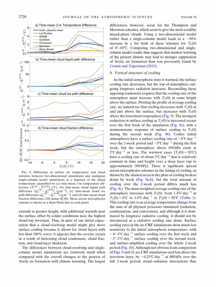
extends to greater height, with additional warmth near

the surface offset by colder conditions near the highest

cloud-top inversion. Thus, in spite of our initial expec-

tation that a cloud-resolving model might give more

surface cooling because it allows for cloud layers with

less than 100% cover, it appears that the reverse occurs

as a result of increasing cloud condensate, cloud frac-

tion, and cloud-layer thickness.

The differences between cloud-resolving and single-

column model simulations are relatively small when

compared with the overall changes to the process of

Arctic air formation with climate warming. The largest

differences, however, occur for the Thompson and

Morrison schemes, which seem to give the most credible

mixed-phase clouds. Using a two-dimensional model

rather than a single-column model leads to a ;50%

increase in g for both of these schemes for T2(0)

of 08–108C. Comparing two-dimensional and single-

column model results thus suggests that modest warming

of the present climate may lead to stronger suppression

of Arctic air formation than was previously found by

Cronin and Tziperman (2015).

b. Vertical structure of cooling

As the initial atmospheric state is warmed, the surface

cooling rate decreases, but the top-of-atmosphere out-

going longwave radiation increases. Reconciling these

opposing tendencies requires that the cooling rate of the

atmosphere must increase with T2(0) at some height

above the surface. Plotting the profile of average cooling

rate, we indeed see that cooling decreases with T2(0) at

and just above the surface, but increases with T2(0)

above the lowermost troposphere (Fig. 9). The strongest

reduction in surface cooling as T2(0) is increased occurs

over the first week of the simulation (Fig. 9a), with a

nonmonotonic response of surface cooling to T2(0)

during the second week (Fig. 9b). Colder initial

atmospheres have a surface cooling rate of ;48Cday21

over the 2-week period and ;58Cday21 during the first

week, but the atmosphere above 850 hPa cools at

28Cday21 or less. The warmest cases [T2(0)5 208C]have a cooling rate of about 28Cday21 that is relatively

constant in time and height over a deep layer (up to

approximately 300hPa). There is significant spread

across microphysics schemes in the timing of cooling, as

shown by the shaded areas in the plots of cooling broken

down by week (Fig. 9a,b), but the total amount of

cooling over the 2-week period differs much less

(Fig. 9c). The mass-weighted average cooling rate of the

atmosphere increases with T2(0), from 1.48Cday21 at

T2(0)5 08C to 1.88Cday21 at T2(0)5 208C (Table 1).

This cooling rate is an average temperature change from

the sum of all physical processes simulated (radiation,

condensation, and convection), and although it is dom-

inated by longwave radiative cooling, it should not be

interpreted as a radiative cooling rate alone. Surface

cooling rates in the no-CRF simulations show much less

sensitivity to the initial atmospheric temperature, with

;48–58Cday21 surface cooling over the first week and

;28–38Cday21 surface cooling over the second week,

and surface-amplified cooling over the whole 2-week

period (Fig. 10). Although not obvious from comparison

of Figs. 9 and 10, no-CRF simulations cool less above the

inversion layer, by ;0.258Cday21 at 800 hPa over the

full 2-week period; cloud–radiation interactions thus

FIG. 8. Difference in surface air temperature and cloud

statistics between two-dimensional simulations and analogous

single-column model simulations as a function of the initial

temperature, quantified by (a) time-mean 2-m temperature dif-

ference (T22D 2T2

SCM) (8C), (b) time-mean cloud liquid path

difference (cqcl2D

2cqclSCM

) (g m22), (c) time-mean cloud ice

path difference (cqci2D

2cqciSCM

) (g m22), and (d) time-mean cloud

fraction difference (2D minus SCM). Mean across microphysics

schemes is shown as a thick black line in each panel.


weaken the surface inversion but shift cooling upward,

to the tops of optically thick clouds, or to the whole layer

spanned by optically thin clouds. An upward shift and

increase in magnitude of mid- and upper-tropospheric

cooling with warming of the initial atmosphere is seen in

simulations with and without cloud–radiation in-

teractions (cf. Figs. 9 and 10 above 600 hPa).

The energy loss of the atmosphere and surface by

radiation to space can be divided into contributions

from changes in internal heat, latent, and gravitational

potential energy of the atmosphere and changes in

heat content of the surface (Table 1; angle brackets

indicate mass-weighted vertical integrals). Condensa-

tion (LyDhqyi/Dt) plays an increasingly important role in

the column energy budget at the warmest temperatures,

amounting to ;40Wm22 of heating in the warmest

cases. For extremely warm initial temperatures, the role

of condensation alone in increasing the effective heat

capacity of the atmosphere could lead to a reduction in

average tropospheric cooling rates with increasing T2(0)

(Cronin and Emanuel 2013), but our simulations do not

reach that limit, in part because our initial soundings are

rather dry. Note that changes in internal heat energy

(cyDhTi/Dt) and gravitational potential energy

(Dhgzi/Dt) of the column do not sum to cpDhTi/Dt, be-cause the upper bound of integration is only ;15 km,

and the equality only holds for a full column integral

(e.g., Peixoto andOort 1992, chapter 13). Loss of heat by

the surface, CSDTS/Dt, supplies &10Wm22 to the at-

mosphere; the magnitude of this term is limited because

the surface heat capacity is small by design (CS 5 2.1 3105 Jm22K21).

c. Top-of-atmosphere radiation and feedbacks

To attempt to compare our results with the feedbacks

diagnosed from global climate models (e.g., Pithan and

Mauritsen 2014), we can analyze how top-of-

atmosphere outgoing longwave radiation (OLR) de-

pends on surface temperature. The main idea is similar

to a climate model feedback analysis: that the derivative

of OLR with respect to TS is a measure of the total ra-

diative feedback, or how strongly top-of-atmosphere

energy loss tends to damp surface warming. Because our

model for Arctic air formation is an idealized depiction

of a complex transient process, this analysis is not

equivalent to a climate model feedback analysis, and we

do not decompose the sensitivity of OLR to surface

temperature TS into specific feedbacks: for example,

Planck, lapse rate, water vapor, and cloud (such a de-

composition would also require additional radiative

transfer calculations outside of WRF). We infer from

this analysis that there are strong positive cloud and

clear-sky feedbacks associated with suppression of

Arctic air formation that make dOLR/dTSmuch smaller

FIG. 9. Vertical profiles of total cooling rate averaged acrossmicrophysics schemes, as a function of initial 2-m air temperature for (a) the

first week, (b) the second week, and (c) both weeks. Solid lines represent averages across microphysics schemes, and the shaded area

indicates the spread across microphysics schemes (plus and minus one standard deviation).


in magnitude (less negative) for the time-mean atmo-

spheric states (during the process of Arctic air forma-

tion) as compared to the initial atmospheric states.

Figure 11a shows the surface temperature de-

pendence of three choices of OLR: initial OLR(0)

plotted against initial surface temperature, time-mean

clear-sky OLRclear plotted against time-mean surface

temperature, and time-mean all-sky OLR plotted

against time-mean surface temperature (values also

given in Table 1). A blackbody with temperature 258Cless than the surface is also plotted for reference as an

example with only the Planck feedback present. De-

noting the negative slope of OLRwith respect to surface

temperature as a feedback, we then also have three

different feedback metrics for our simulations, corre-

sponding to each choice of OLR:

l(0)52dOLR(0)

dTS(0)

lclear

52dOLR

clear

dTS

l52dOLR

dTS

.

(4)

These feedback parameters are plotted with negative

signs and represent a stabilizing total longwave feedback

in all cases: a warmer atmosphere and surface lead to

more OLR (Fig. 11b). The contrast in the feedback

parameter l, and its temperature dependence, between

the time-mean and initial OLR values provides a mea-

sure of how the suppression of cold-air formation alters

the local top-of-atmosphere longwave feedback. We

wish to emphasize a few features of Fig. 11b:

d The longwave feedback in the initial state l(0) in-

creases in magnitude from 22.2Wm22K21 for the

coldest initial temperatures to22.8Wm22K21 for the

warmest, presumably because of negative Planck and

lapse-rate radiative feedbacks, which increase in

strength with warming of the initial state.d The longwave clear-sky feedback in the time-mean state

lclear has a near-constant value ;21.7Wm22K21.

The smaller magnitude of lclear relative to l(0)—

by ;0.5Wm22 K21 in the range of overlapping

temperature—indicates that there are positive clear-

sky OLR feedbacks associated with the suppression of

Arctic air formation. We interpret this offset between

lclear and l(0) as primarily a positive lapse-rate

feedback, though we cannot rule out a water vapor

feedback component.d The longwave all-sky feedback in the time-mean state

l decreases in magnitude from 21.9Wm22K21 for

the coldest initial temperatures to20.9Wm22K21 for

the warmest. The smaller magnitude of the feedback l

FIG. 10. Vertical profiles of total cooling rate for clear-sky radiation simulations (no-CRF) as a function of initial 2-m air temperature for

(a) the first week, (b) the second week, and (c) both weeks.


with warming is due to a positive top-of-atmosphere

cloud longwave feedback that rapidly increases to

;1Wm22 K21 for the warmest initial conditions

(cf. l and lclear in Fig. 11b).

The strong top-of-atmosphere cloud feedback under

warm conditions shown in Fig. 11b can also be inferred

from time-mean top-of-atmosphere cloud radiative

forcing, which is generally small compared to the surface

cloud radiative forcing (and can even be negative), but

which increases rapidly with warming for warm initial

atmospheres (Table 1, bottom two rows). From a con-

ventional top-of-atmosphere standpoint, clouds may

thus act as a stronger positive feedback than was re-

alized by Cronin and Tziperman (2015). Our results thus

support the potentially important role of positive top-of-

atmosphere longwave cloud feedback, particularly in

much warmer climates (e.g., Abbot et al. 2009).

d. Treatment of the surface and other limitations

The surface in our model is treated very simply, es-

sentially as a heat-storing slab that is dragged along with

the atmosphere as it moves. By using identical values of

TS(0) and T2(0) and giving the surface a relatively low

heat capacity, we have tried to minimize biases in sen-

sitivity g52›DT2/›T2(0) that might be related to the

surface, although one clear limitation of this work is that

properties of the surface do not change at all with tem-

perature, even though major changes in real surface

properties occur across the freezing point. Cronin and

Tziperman (2015) found that a surface with higher heat

capacity leads to smaller values of g, whereas a surface

with a lower heat capacity leads to a larger g. We

speculate that greater surface heat capacity will gener-

ally make surface temperatures less sensitive to changes

in initial atmospheric state. This would have implica-

tions for previous work by Curry (1983), Pithan et al.

(2014), and Pithan et al. (2016), who used a sea ice–like

surface, with a prescribed thickness and temperature

profile. Such a structural choice makes sense for ex-

ploring Arctic air formation in the present climate but

likely makes g smaller than in our work, because ice

with a prescribed temperature that is independent of the

initial 2-m air temperature will conduct heat out of a

warm initial atmosphere or into a cold initial

atmosphere.

Our defaultmodel resolution (Dx,Dz)5 (100, 50)mhas

allowed us to run a large number of simulations across

different microphysics schemes and temperatures but

may be insufficient to fully resolve the liquid layer at the

top of Arctic mixed-phase clouds (e.g., Ovchinnikov

et al. 2014) and the sharpness of inversions that form

near stratus cloud tops (e.g., Blossey et al. 2013). Sen-

sitivity tests with varied resolution using the Lin–Purdue

scheme at T2(0) of 08 and 208C show that altering the

horizontal resolution by a factor of 2 typically leads to a

change of a few watts per square meter in surface cloud

forcing and ;18C in time-mean surface air temperature

and that decreasing the resolution for a cold initial

state can completely suppress the low-level turbulence

(Table 2). Increasing vertical resolution leads to surface

warming for T2(0)5 208C but to surface cooling for

T2(0)5 08C. This reversal occurs because the cloudy

state dominates in the warm simulation, but the clear

state dominates in the cold simulation, and its sharp

surface inversions are strengthened at high vertical

resolution. The Thompson and Morrison schemes,

which simulate better mixed-phase clouds at low

FIG. 11. (a) OLR as a function of surface temperature for initial

conditions [OLR(0)], time-mean values (OLR), and time-mean

clear-sky values (OLRclear). (b) Feedbacks based on slopes of OLR

[from (a)] with respect to TS. Progressively less negative values of

lclear and l relative to l(0) in (b) indicate positive cloud and clear-

sky feedbacks associated with suppression of Arctic air formation

from warmer initial states. A blackbody with temperature 258Clower than the surface (TS 2 25) is shown as dotted lines to provide

reference values for (a) OLR and (b) the Planck feedback by itself.


temperature, might be more sensitive to resolution for

cold initial states. Use of two-dimensional rather than

three-dimensional geometry is also a limitation of this

study; we originally imagined that the upscale cascade of

turbulent kinetic energy in two dimensions might allow

for larger-scale circulations to develop and disrupt lay-

ered clouds, but it is not clear to what extent this oc-

curred in any of our simulations.

Another limitation of thiswork is the lack of large-scale

subsidence or wind shear. Moderate subsidence in single-

column simulations of Cronin and Tziperman (2015) was

found to limit the upward growth of the cloud layer but

did little tomodify the suppression ofArctic air formation

in a warmer initial atmosphere; we anticipate similar

sensitivity to subsidence in the cloud-resolving model

used here. A stochastically varying vertical velocity pro-

file that includes stronger ascent and stronger subsidence,

as in Brient and Bony (2013), might provide a stronger

and more realistic test of our mechanism than steady

subsidence. Regarding wind shear, we expect more rapid

horizontal advection of air aloft than near the surface, so

realistic vertical shear would likely lead to less cooling in

the mid- and upper troposphere as an air mass traverses a

continent than we have simulated here. The 2-week time

period during which we follow the cold air formation

process is also somewhat arbitrary and should be in-

formed by investigation of the observed time scales of

continental traversal for air parcels in the lower tropo-

sphere and projections of how these time scales may

change with warming. Recent work by Woods and

Caballero (2016) has suggested a link between observed

Arctic warming and increasing frequency of injection

events of very warm and moist air into the polar region:

a result consistent with the ideas presented in this paper.

Questions about the role of large-scale dynamics—both

vertical advection and the statistics of horizontal flow—

point to investigation of cold-air formation in a global

climate model as a productive future research direction.

An additional limitation was noted above: in the

version of WRF we use, the coupling between radiation

and microphysics is incomplete. Only the total liquid

and ice content in each column and vertical level are

passed from the microphysics scheme to the radiation

scheme, and the radiation scheme makes its own as-

sumptions about cloud particle sizes. The spread across

microphysics schemes shown here thus includes

temperature-dependent differences in liquid condensate

fraction and microphysical removal rates but does not

include the coupling between varying particle sizes and

radiation. Investigation of cloud ice effective radii in the

Thompson and Morrison scheme simulations (not

shown) reveals large differences between the two

schemes but only weak sensitivity to T2(0) in each. Lack

of temperature dependence within each scheme is re-

assuring for our overall mechanism for suppression of

Arctic air formation, but the large difference between

schemes indicates that we have underestimated the

spread in cooling rates that would occur for complete

coupling of radiation and microphysics. Finally, we do

not include in our simulations any link between aerosols

and clouds or precipitation, although interactions be-

tween aerosol, cloud, and precipitation are likely im-

portant for determining cloud particle size and lifetime

in the real Arctic (Mauritsen et al. 2011; Solomon

et al. 2015).

5. Conclusions

We have used a two-dimensional cloud-resolving con-

figuration of the WRF Model to investigate the idea that

Arctic air formation is suppressed in warmer climates.

Our results indicate that warming of the initial state leads

to substantial inhibition of Arctic air formation via the

development of optically thick low-level liquid clouds

that hamper surface radiative cooling and are consistent

with single-column model simulations in Cronin and

Tziperman (2015). The 2-week averaged cooling de-

creases by roughly 0.68C for each degree warming of the

initial state at initial air temperatures near 08C, and this

amplification factor rises for very warm initial air

TABLE 2. Comparison of simulations with varied grid spacing. Metrics for comparison are the time-mean 2-m air temperature (T2; 8C),the time-mean surface cloud radiative forcing (CRFS; Wm22), and the time-mean standard deviation of the instantaneous zonal wind,

averaged over levels between 1000 and 850 hPa (su; m s21). Values in parentheses indicate deviations from the respective control sim-

ulation. Simulations shown use the Lin–Purdue microphysics scheme, with initial 2-m temperatures of T2(0)5 08C and T2(0)5 208C.

Simulation Grid spacing (Dx, Dz) (m)

T2(0)5 08C T2(0)5 208C

T2 (8C) CRFS (Wm22) su (m s21) T2 (8C) CRFS (Wm22) su (m s21)

Control (100, 50) 238.83 15.34 0.010 3.63 61.71 0.204

53 horizontal (500, 50) 238.5 (0.28) 11.5 (23.87) 0.001 (20.009) 2.0 (21.58) 58.9 (22.85) 0.169 (20.035)

2.53 horizontal (250, 50) 238.5 (0.33) 11.5 (23.85) 0.001 (20.009) 2.2 (21.45) 59.2 (22.48) 0.168 (20.036)

1/23 horizontal (50, 50) 237.3 (1.54) 18.1 (2.81) 0.019 (0.010) 4.0 (0.36) 62.9 (1.22) 0.183 (20.021)

23 vertical (100, 100) 237.1 (1.68) 16.2 (0.90) 0.015 (0.006) 2.6 (21.03) 57.5 (24.24) 0.173 (20.030)

1/23 vertical (100, 25) 239.5 (20.67) 16.1 (0.78) 0.026 (0.016) 3.7 (0.11) 62.9 (1.20) 0.208 (0.004)


temperatures to as much as 1.78C of reduced cooling for

each degree warming of the initial state. These results are

robust across several different cloud microphysics

schemes, but suppression of cold-air formation is stronger

in the schemes that produce the most credible mixed-

phase clouds and also more sensitive in these schemes to

the use of a two-dimensional model rather than a single-

column model. Low-level clouds in the two-dimensional

simulations growmore rapidly, extend to greater altitude,

and persist longer as compared to analogous single-

column simulations, which increases the strength of the

cloud feedback. The greater altitude reached and faster

growth of the lower-tropospheric cloud layer appear re-

lated to cloud-top entrainment and turbulence, which is

not resolved in the single-column model.

This paper has found that resolving smaller-scale pro-

cesses, especially convection and turbulence at scales of

;100 m–10km, strengthens the results of Cronin and

Tziperman (2015). Many questions for future research on

Arctic air formation relate to larger spatial scales and the

interaction of Arctic air formation with the general cir-

culation of the mid- and high-latitude atmosphere. How

does the upward shift in cooling during the formation of

cold air affect mid- and high-latitude dynamics? What

pressure levels in the Arctic atmosphere are most linked

to extreme cold outbreaks inmidlatitudes?How robust is

the low-cloud insulation mechanism to full three-

dimensional wind variability in a global model? What is

the joint probability density function of age of terrestrial

air and sea surface temperature last encountered, and

how does this joint distribution change with global

warming? Addressing these questions may offer new

ways of understanding Arctic amplification and its cou-

pling to changes in midlatitude extreme weather.

Acknowledgments. This work was supported by a

Harvard undergraduate PRISE fellowship (HL), by a

NOAA Climate and Global Change Postdoctoral Fel-

lowship (TWC), by the Harvard University Center for

the Environment (TWC), and by the NSF climate dy-

namics program under Grant AGS-1303604 (ET). ET

thanks the Weizmann institute for its hospitality during

parts of this work.We thank three anonymous reviewers

for thorough and helpful comments that helped to

improve the manuscript.

APPENDIX

Cloud Microphysics Schemes

We use six different microphysics schemes in this

paper, denoted the Lin–Purdue, WSM6, Goddard,

Thompson, Morrison, and Stony Brook schemes. Each

is described in its own subsection below, emphasizing

processes that produce and consume cloud ice (critical

for understanding mixed-phase clouds). Most of the

models are bulk schemes that use a single prognostic

variable (mass mixing ratio) to model six classes of wa-

ter: vapor, cloud liquid, cloud ice, rain, snow, and

graupel. Exceptions to this single-moment 6-class de-

fault are noted below in the description of each scheme.

Previous work highlights the importance of liquid–ice

partitioning as a function of temperature in determining

the magnitude of low-cloud optical thickness feedback

over the Southern Ocean in global climate models

(McCoy et al. 2015). The dependence of liquid cloud

condensate fraction on temperature is an informative

emergent property of both the microphysics scheme and

the model setup (Fig. A1) and has also been shown to be

related to model biases in mixed-phase clouds (Pithan

et al. 2014). As in McCoy et al. (2015), we denote the

glaciation temperature for each scheme as T50–50, or the

temperature at which half of cloud water is ice and half is

liquid. Curves in Fig. A1 were calculated by aggregating

the liquid cloud condensate fraction for all model grid-

points with at least 1024 gkg21 of total cloud condensate

among the simulations with initial surface temperatures

in f2108, 258, 08, 58, 108, 158, 208gC into bins of width

18C. The glaciation temperatures in our simulations are

around 158C higher than the near-global observations of

Hu et al. (2010) and themultimodelmean inMcCoy et al.

(2015), and we also find amore rapid liquid–ice transition

with temperature than in observations (Fig. A1). The

implications of these biases are unclear; McCoy et al.

(2015) suggest that higher glaciation temperature corre-

sponds to a stronger cloud optical thickness feedback

over the Southern Ocean, but clouds in our model setup

often form at a much lower temperature than experi-

enced in the lower troposphere over the SouthernOcean.

We speculate that lowering the glaciation temperature

of a specific scheme might lead to larger cloud optical

thickness changes with warming at lower T2(0), perhaps

shifting curves in Figs. 6 and 7 to the left.

a. Lin–Purdue scheme

The Lin–Purdue scheme is described in Lin et al.

(1983) and cloud liquid and cloud ice microphysics are

described in more detail in Hsie et al. (1980). Cloud ice

in the model is produced primarily by supersaturation

adjustment, with the fraction of supersaturation parti-

tioned into cloud ice varying linearly from 0 at 08C to 1

at 2258C (e.g., at 2108C, 40% of any vapor supersatu-

ration in a grid cell would be converted to cloud ice,

and the other 60% to cloud liquid) and supersaturation

calculated as a linear mix of that over liquid and ice

with the same temperature-dependent weighting. This


method of supersaturation adjustment has the un-

realistic consequence that all newly formed clouds be-

low 08C contain at least some ice. Offline calculations

show that the production of cloud ice from cloud liquid

by depositional growth—an arrow shown in Fig. 1 of Lin

et al. (1983)—is entirely negligible. This simple linear

ramp is responsible for the near-linear dependence of

liquid condensate fraction on temperature in the Lin–

Purdue scheme (linear ramp shown as a dotted black

line in Fig. A1), with T50–50 5 213.28C just below the

midpoint of the mixed-phase range. Liquid condensate

fraction lies above this dotted line in Fig. A1 for tem-

peratures between about 2108 and 08C because the

model implementation of the Bergeron process leads to

more rapid removal of cloud ice than it does of cloud

liquid, often leading to supercooled liquid clouds that

have snowed out all of their ice.

b. WSM6 scheme

The WSM6 scheme is described in Hong and Lim

(2006), but many essential details of the cloud ice

scheme are presented in Hong et al. (2004). Cloud ice is

produced rapidly by transfer from the vapor phase, both

onto existing particles and forming new particles, even

at temperatures just below freezing. If little existing ice

present, then the scheme produces ice by initiation of

new particles, at a rate sufficient to deplete the super-

saturation over ice in &1500 s at all temperatures below

freezing. If existing cloud ice is present, then vapor de-

position onto existing ice particles can be a faster pro-

cess, especially at temperatures slightly below freezing.

This aggressive formation of cloud ice from vapor is

responsible for the extremely high glaciation tempera-

ture T50–50 5 20.58C in the WSM6 scheme. WSM6 also

maintains clouds with the largest ice path, in part be-

cause autoconversion of cloud ice to snow has a high

threshold of 0.08/r g kg21, but also because the param-

eterization of the Bergeron process does not directly

transfer mass from cloud ice to snow.

c. Goddard scheme

The Goddard scheme is described in Tao et al. (1989)

and Tao et al. (2003). Cloud ice production occurs by a

combination of direct deposition from vapor and by the

parameterization of the Bergeron process, which trans-

fers mass directly from cloud liquid to ice and has an

increase in its rate coefficient by a factor of ;500 as

temperatures drop from 288 to 2158C. This rapid in-

crease in conversion rate from cloud liquid to cloud ice

with cooling is likely responsible for the value of the

glaciation temperature T50–50 5 212.28C, as well as thesharpness of the transition from liquid to ice clouds in

the Goddard scheme (Fig. A1). The Goddard scheme

has an even larger autoconversion threshold than the

WSM6 scheme for forming snow from cloud ice

(0.6 g kg21), but it also has rapid transfer of mass from

cloud ice to snow through the Bergeron process; the

competition of these processes leads to it being the

scheme with the second-largest cloud ice path.

d. Thompson scheme

The Thompson scheme is described in Thompson et al.

(2008) and simulates two-moment rain and cloud ice (i.e.,

it tracks both number and mass mixing ratio variables for

cloud ice and rain). The Thompson scheme also has the

lowest glaciation temperature ofT50–505217.58C, whichis related both to its maintenance of supercooled water

and its very low cloud ice mixing ratios. Two-moment

cloud ice makes it far more difficult to disentangle the

dominant sources and sinks of cloud ice by offline coding

of process rates. Simulated cloud ice production includes

heterogeneous nucleation of new ice particles at ice

supersaturation greater than 25% or temperatures less

than 2128C and supersaturation over liquid, deposition

from vapor onto existing particles, freezing of cloud liq-

uid, freezing of small raindrops, and ice multiplication

from rime splintering. The rate of cloud ice production

from freezing of cloud liquid increases exponentially

with supercooling and with the liquid droplet volume,

following Bigg (1953).

e. Morrison scheme

The Morrison scheme is described in Morrison et al.

(2009) and in more detail by Morrison and Pinto (2005),

FIG. A1. Dependence of liquid condensate fraction on temper-

ature (as in McCoy et al. 2015), taken from simulations with T2(0)

in f2108, 258, 08, 58, 108, 158, 208gC and averaged over all time

intervals and vertical levels where total cloud condensate is greater

than 1024 g kg21. The fit to global satellite observations from (1)

and (2) of Hu et al. (2010) is also shown as a thick gray line.


and it has two-moment rain, snow, graupel, and cloud ice

(i.e., it tracks both number and mass mixing ratio vari-

ables for rain, snow, graupel, and cloud ice). Despite the

high glaciation temperature of T50–50 5 24.88C, thescheme is nonetheless able to produce layers of super-

cooled liquid cloud below 2208C, especially at low

T2(0). As with the Thompson scheme, two-moment

variables make it difficult to disentangle dominant

sources and sinks of cloud ice. Simulated ice production

includes heterogeneous nucleation of new ice particles,

deposition from vapor onto existing particles, freezing of

cloud liquid (similar to the Thompson scheme),

accretion of cloud liquid droplets by falling ice, and

distinct ice multiplication pathways from cloud liquid–

snow, cloud liquid–graupel, rain–snow, and rain–graupel

interactions.

f. Stony Brook scheme

The Stony Brook scheme is described in Lin and Colle

(2011) and is a direct descendant of the Lin–Purdue

scheme. It has a near-identical treatment of cloud liquid

and ice physics, and the major difference from the Lin–

Purdue scheme is that the prognostic graupel variable is

replaced by a continuous riming intensity variable for

falling ice. The liquid condensate fraction curve is al-

most identical to that of the Lin–Purdue scheme in

Fig. A1, with T50–50 5 212.68C.

REFERENCES

Abbot, D. S., M. Huber, G. Bosquet, and C. Walker, 2009: High-

CO2 cloud radiative forcing feedback over both land and

ocean in a global climate model. Geophys. Res. Lett., 36,

L05702, doi:10.1029/2008GL036703.

Alexeev, V. A., and C. H. Jackson, 2013: Polar amplification: Is

atmospheric heat transport important? Climate Dyn., 41, 533–

547, doi:10.1007/s00382-012-1601-z.

Bigg, E. K., 1953: The formation of atmospheric ice crystals by the

freezing of droplets. Quart. J. Roy. Meteor. Soc., 79, 510–519,

doi:10.1002/qj.49707934207.

Blossey, P. N., andCoauthors, 2013:Marine low cloud sensitivity to

an idealized climate change: The CGILS LES in-

tercomparison. J. Adv. Model. Earth Syst., 5, 234–258,

doi:10.1002/jame.20025.

Brient, F., and S. Bony, 2013: Interpretation of the positive low-

cloud feedback predicted by a climate model under global

warming. Climate Dyn., 40, 2415–2431, doi:10.1007/

s00382-011-1279-7.

Chylek, P., C. K. Folland, G. Lesins, M. K. Dubey, and M. Wang,

2009: Arctic air temperature change amplification and the

Atlantic multidecadal oscillation. Geophys. Res. Lett., 36,

L14801, doi:10.1029/2009GL038777.

Cronin, T. W., and K. A. Emanuel, 2013: The climate time scale in

the approach to radiative-convective equilibrium. J. Adv.

Model. Earth Syst., 5, 843–849, doi:10.1002/jame.20049.

——, and E. Tziperman, 2015: Low clouds suppress Arctic air

formation and amplify high-latitude continental winter

warming. Proc. Natl. Acad. Sci. USA, 112, 11490–11495,

doi:10.1073/pnas.1510937112.

Curry, J., 1983: On the formation of continental polar air. J. Atmos.

Sci., 40, 2278–2292, doi:10.1175/1520-0469(1983)040,2278:

OTFOCP.2.0.CO;2.

——, W. B. Rossow, D. Randall, and J. L. Schramm, 1996:

Overview of Arctic cloud and radiation characteristics.

J. Climate, 9, 1731–1764, doi:10.1175/1520-0442(1996)009,1731:

OOACAR.2.0.CO;2.

Emanuel, K., 2008: Back to Norway: An essay. Meteor. Monogr.,

33, 87–96, doi:10.1175/0065-9401-33.55.87.Greenwood, D. R., and S. L. Wing, 1995: Eocene continental

climates and latitudinal temperature gradients. Geology,

23, 1044–1048, doi:10.1130/0091-7613(1995)023,1044:

ECCALT.2.3.CO;2.

Hartmann, D. L., and Coauthors, 2013: Observations: Atmosphere

and surface. Climate Change 2013: The Physical Science Basis,

T. F. Stocker et al., Eds., Cambridge University Press, 159–

186. [Available online at http://www.climatechange2013.org/

images/report/WG1AR5_Chapter02_FINAL.pdf.]

Holland, M., and C. Bitz, 2003: Polar amplification of climate

change in coupled models. Climate Dyn., 21, 221–232,

doi:10.1007/s00382-003-0332-6.

Hong, S.-Y., and J.-O. Lim, 2006: The WRF single-moment 6-class

microphysics scheme (WSM6). J.KoreanMeteor. Soc.,42, 129–151.

——, J. Dudhia, and S.-H. Chen, 2004: A revised approach to

ice microphysical processes for the bulk parameterization

of clouds and precipitation. Mon. Wea. Rev., 132, 103–120,

doi:10.1175/1520-0493(2004)132,0103:ARATIM.2.0.CO;2.

——, Y. Noh, and J. Dudhia, 2006: A new vertical diffusion

package with explicit treatment of entrainment processes.

Mon. Wea. Rev., 134, 2318–2341, doi:10.1175/MWR3199.1.

Hsie, E.-Y., R. D. Farley, and H. O. Orville, 1980: Numerical

simulation of ice-phase convective cloud seeding. J. Appl.

Meteor., 19, 950–977, doi:10.1175/1520-0450(1980)019,0950:

NSOIPC.2.0.CO;2.

Hu, Y., S. Rodier, K.-M. Xu,W. Sun, J. Huang, B. Lin, P. Zhai, and

D. Josset, 2010: Occurrence, liquid water content, and fraction

of supercooled water clouds from combined CALIOP/IIR/

MODIS measurements. J. Geophys. Res., 115, D00H34,

doi:10.1029/2009JD012384.

Iacono, M., J. S. Delamere, E. J. Mlawer, M. W. Shephard,

S. A. Clough, and W. D. Collins, 2008: Radiative forcing by long-

lived greenhouse gases: Calculations with the AER radiative

transfer models. J. Geophys. Res., 113, D13103, doi:10.1029/

2008JD009944.

Kapsch,M.-L., R. Graversen, andM. Tjernstrom, 2013: Springtime

atmospheric energy transport and the control of Arctic sum-

mer sea-ice extent. Nat. Climate Change, 3, 744–748,

doi:10.1038/nclimate1884.

Lin, Y., and B. A. Colle, 2011: A new bulk microphysical scheme

that includes riming and temperature-dependent ice char-

acteristics. Mon. Wea. Rev., 139, 1013–1035, doi:10.1175/

2010MWR3293.1.

Lin, Y.-L., R. Farley, and H. Orville, 1983: Bulk parameterization

of the snow field in a cloud model. J. Climate Appl.

Meteor., 22, 1065–1092, doi:10.1175/1520-0450(1983)022,1065:

BPOTSF.2.0.CO;2.

Mauritsen, T., and Coauthors, 2011: AnArctic CCN-limited cloud-

aerosol regime.Atmos. Chem. Phys., 11, 165–173, doi:10.5194/

acp-11-165-2011.

McCoy, D. T., D. L. Hartmann, M. D. Zelinka, P. Ceppi, and D. P.

Grosvenor, 2015: Mixed-phase cloud physics and Southern


http://dx.doi.org/10.1029/2008GL036703

http://dx.doi.org/10.1007/s00382-012-1601-z

http://dx.doi.org/10.1002/qj.49707934207

http://dx.doi.org/10.1002/jame.20025

http://dx.doi.org/10.1007/s00382-011-1279-7

http://dx.doi.org/10.1007/s00382-011-1279-7

http://dx.doi.org/10.1029/2009GL038777

http://dx.doi.org/10.1002/jame.20049

http://dx.doi.org/10.1073/pnas.1510937112

http://dx.doi.org/10.1175/1520-0469(1983)040<2278:OTFOCP>2.0.CO;2

http://dx.doi.org/10.1175/1520-0469(1983)040<2278:OTFOCP>2.0.CO;2

http://dx.doi.org/10.1175/1520-0442(1996)009<1731:OOACAR>2.0.CO;2

http://dx.doi.org/10.1175/1520-0442(1996)009<1731:OOACAR>2.0.CO;2

http://dx.doi.org/10.1175/0065-9401-33.55.87

http://dx.doi.org/10.1130/0091-7613(1995)023<1044:ECCALT>2.3.CO;2

http://dx.doi.org/10.1130/0091-7613(1995)023<1044:ECCALT>2.3.CO;2

http://www.climatechange2013.org/images/report/WG1AR5_Chapter02_FINAL.pdf

http://www.climatechange2013.org/images/report/WG1AR5_Chapter02_FINAL.pdf

http://dx.doi.org/10.1007/s00382-003-0332-6

http://dx.doi.org/10.1175/1520-0493(2004)132<0103:ARATIM>2.0.CO;2

http://dx.doi.org/10.1175/MWR3199.1

http://dx.doi.org/10.1175/1520-0450(1980)019<0950:NSOIPC>2.0.CO;2

http://dx.doi.org/10.1175/1520-0450(1980)019<0950:NSOIPC>2.0.CO;2

http://dx.doi.org/10.1029/2009JD012384

http://dx.doi.org/10.1029/2008JD009944

http://dx.doi.org/10.1029/2008JD009944

http://dx.doi.org/10.1038/nclimate1884

http://dx.doi.org/10.1175/2010MWR3293.1


http://dx.doi.org/10.1175/1520-0450(1983)022<1065:BPOTSF>2.0.CO;2

http://dx.doi.org/10.1175/1520-0450(1983)022<1065:BPOTSF>2.0.CO;2

http://dx.doi.org/10.5194/acp-11-165-2011


Ocean cloud feedback in climate models. J. Geophys. Res.

Atmos., 120, 9539–9554, doi:10.1002/2015JD023603.

Morrison, H., and J. O. Pinto, 2005: Mesoscale modeling of

springtime Arctic mixed-phase stratiform clouds using a new

two-moment bulk microphysics scheme. J. Atmos. Sci., 62,

3683–3704, doi:10.1175/JAS3564.1.

——, G. Thompson, and V. Tatarskii, 2009: Impact of cloud mi-

crophysics on the development of trailing stratiform pre-

cipitation in a simulated squall line: Comparison of one- and

two-moment schemes. Mon. Wea. Rev., 137, 991–1007,

doi:10.1175/2008MWR2556.1.

——, G. de Boer, G. Feingold, J. Harrington, M. Shupe, and

K. Sulia, 2012: Resilience of persistent Arctic mixed-phase

clouds. Nat. Geosci., 5, 11–17, doi:10.1038/ngeo1332.

Mortin, J., G. Svensson, R. Graversen,M.-L. Kapsch, J. C. Stroeve,

and L. N. Boisvert, 2016: Melt onset over Arctic sea ice con-

trolled by atmospheric moisture transport. Geophys. Res.

Lett., 43, 6636–6642, doi:10.1002/2016GL069330.

Ovchinnikov, M., and Coauthors, 2014: Intercomparison of large-

eddy simulations of Arctic mixed-phase clouds: Importance of

ice size distribution assumptions. J. Adv. Model. Earth Syst., 6,

223–248, doi:10.1002/2013MS000282.

Overland, J. E., and P. S. Guest, 1991: The Arctic snow and air

temperature budget over sea ice during winter. J. Geophys.

Res., 96, 4651–4662, doi:10.1029/90JC02264.

Peixoto, J. P., and A. H. Oort, 1992: Physics of Climate. Springer-

Verlag, 520 pp.

Pithan, F., and T. Mauritsen, 2014: Arctic amplification dominated

by temperature feedbacks in contemporary climate models.

Nat. Geosci., 7, 181–184, doi:10.1038/ngeo2071.——, B. Medeiros, and T. Mauritsen, 2014: Mixed-phase clouds

cause climate model biases in Arctic wintertime tempera-

ture inversions. Climate Dyn., 43, 289–303, doi:10.1007/

s00382-013-1964-9.

——, and Coauthors, 2016: Select strengths and biases of models

representing the Arctic winter boundary layer over sea ice:

The Larcform 1 single column model intercomparison.

J. Adv. Model. Earth Syst., 8, 1345–1357, doi:10.1002/

2016MS000630.

Sedlar, J., andCoauthors, 2011:A transitioningArctic surface energy

budget: The impacts of solar zenith angle, surface albedo, and

cloud radiative forcing. Climate Dyn., 37, 1643–1660,

doi:10.1007/s00382-010-0937-5.

Solomon, A., G. Feingold, and M. D. Shupe, 2015: The role of ice

nuclei recycling in the maintenance of cloud ice in Arctic

mixed-phase stratocumulus. Atmos. Chem. Phys., 15, 10 631–

10 643, doi:10.5194/acp-15-10631-2015.

Stramler, K., A.D.D.Genio, andW.B. Rossow, 2011: Synoptically

driven Arctic winter states. J. Climate, 24, 1747–1762,

doi:10.1175/2010JCLI3817.1.

Tao, W.-K., J. Simpson, and M. McCumber, 1989: An ice-water

saturation adjustment. Mon. Wea. Rev., 117, 231–235,

doi:10.1175/1520-0493(1989)117,0231:AIWSA.2.0.CO;2.

——, and Coauthors, 2003: Microphysics, radiation, and surface

processes in the Goddard Cumulus Ensemble (GCE) model.

Meteor. Atmos. Phys., 82, 97–137, doi:10.1007/s00703-001-0594-7.Thompson, G., P. Fiels, R. Rasmussen, and W. Hall, 2008: Explicit

forecasts of winter precipitation using an improved bulk mi-

crophysics scheme. Part II: Implementation of a new snow

parameterization. Mon. Wea. Rev., 136, 5095–5115, doi:10.1175/2008MWR2387.1.

Tjernstrom, M., and Coauthors, 2015: Warm-air advection, air

mass transformation, and fog causes rapid ice melt. Geophys.

Res. Lett., 42, 5594–5602, doi:10.1002/2015GL064373.

Van Tricht, K., and Coauthors, 2016: Clouds enhance Greenland

ice sheet meltwater runoff. Nat. Commun., 7, 10 266,

doi:10.1038/ncomms10266.

Verlinde, J., M. P. Rambukkange, E. E. Clothiaux, G. M.

McFarquhar, and E. W. Eloranta, 2013: Arctic multilayered,

mixed-phase cloud processes revealed in millimeter-wave

cloud radar Doppler spectra. J. Geophys. Res. Atmos., 118,13 199–13 213, doi:10.1002/2013JD020183.

Wexler, H., 1936: Cooling in the lower atmosphere and the

structure of polar continental air.Mon.Wea. Rev., 64, 122–136,

doi:10.1175/1520-0493(1936)64,122:CITLAA.2.0.CO;2.

Woods, C., and R. Caballero, 2016: The role of moist intrusions in

winter Arctic warming and sea ice decline. J. Climate, 29,

4473–4485, doi:10.1175/JCLI-D-15-0773.1.

Zuidema, P., and R. Joyce, 2008: Water vapor, cloud liquid

water paths, and rain rates over northern high latitude

open seas. J. Geophys. Res., 113, D05205, doi:10.1029/

2007JD009040.


http://dx.doi.org/10.1002/2015JD023603

http://dx.doi.org/10.1175/JAS3564.1


http://dx.doi.org/10.1038/ngeo1332

http://dx.doi.org/10.1002/2016GL069330

http://dx.doi.org/10.1002/2013MS000282

http://dx.doi.org/10.1029/90JC02264

http://dx.doi.org/10.1038/ngeo2071

http://dx.doi.org/10.1007/s00382-013-1964-9

http://dx.doi.org/10.1007/s00382-013-1964-9

http://dx.doi.org/10.1002/2016MS000630

http://dx.doi.org/10.1002/2016MS000630

http://dx.doi.org/10.1007/s00382-010-0937-5


http://dx.doi.org/10.1175/2010JCLI3817.1

http://dx.doi.org/10.1175/1520-0493(1989)117<0231:AIWSA>2.0.CO;2

http://dx.doi.org/10.1007/s00703-001-0594-7



http://dx.doi.org/10.1002/2015GL064373

http://dx.doi.org/10.1038/ncomms10266

http://dx.doi.org/10.1002/2013JD020183

http://dx.doi.org/10.1175/1520-0493(1936)64<122:CITLAA>2.0.CO;2

http://dx.doi.org/10.1175/JCLI-D-15-0773.1

http://dx.doi.org/10.1029/2007JD009040

http://dx.doi.org/10.1029/2007JD009040

Suppression of Arctic Air Formation with Climate Warming ... · PDF fileSuppression of Arctic...

Documents

Transcript of Suppression of Arctic Air Formation with Climate Warming ... · PDF fileSuppression of Arctic...