1

Supporting Information for

Advancement in Liquid Exfoliation of Graphite

through Simultaneously Oxidizing and Ultrasonicating

Ge Shia,b, Andrew Michelmoreb, Jian Jinc, Luhua Lid, Ying Chend, Lianzhou Wange, Hua Yue, Gordon Wallacef, Sanjeev Gambhirf, Shenmin Zhug, Pejman Hojati-Talemib, Jun Ma*a,b

aSchool of Engineering and 2Mawson Institute, University of South Australia, SA5095, AustraliabSuzhou Institute of Nano-Tech and Nano-Bionics, Chinese Academy of Sciences, Suzhou 215123, ChinacInstitute for Frontier Materials, Deakin University, Geelong Waurn Ponds Campus, VIC 3216, AustraliadSchool of Chemical Engineering and AIBN, the University of Queensland, QLD 4072, AustraliaeIntelligent Polymer Research Institute, University of Wollongong, NSW 2500, AustraliafState Key Laboratory of Metal Matrix Composites, Shanghai Jiao Tong University, 200240, China gState Key Laboratory of Metal Matrix Composites, Shanghai Jiao Tong University, 200240, China

1. Experimental setup for oxidi-sonication

Graphite particles were first mixed with acids and potassium permanganate as shown in the

Experiment, and then the mixture was immediately placed into an ultrasonication bath to

simultaneously undertake oxidation and ultrasonication (oxidi-sonication), as shown in Figure S1.

Fig. S1 Ultrasonication bath for simultaneously oxidizing and ultrasonicating graphite

(oxidi-sonication)

Electronic Supplementary Material (ESI) for Journal of Materials Chemistry A.This journal is © The Royal Society of Chemistry 2014

2

2. Comparison of our oxidi-sonication method with the improved Hummer’s method1

In the oxidi-sonication, the acid mixture consists of 26 g phosphoric acid, 6 g sulphuric acid and 0.1

g graphite. After 0.4 g potassium permanganate was added, Mn2O7 formed at a low speed which is

due to phosphoric acid used. The temperature arose slowly and the colour changed to red purple

owing to the dissolution of Mn2O7 (Figure S2 a1). The reaction rate was low, so some potassium

permanganate particles left at the beaker bottom (Figure S2 a2).

a1 a2 a3

b1 b2 b3

Fig. S2 Comparison between our oxidi-sonication method (a) and the improved Hummer’s method (b).

In the improved Hummer’s method, the precursor consists of 0.76 g phosphoric acid, 6.5 g

sulphuric acid and 0.1 g graphite. Following the addition of potassium permanganate (0.6 g),

Mn2O7 formed immediately (Figure S2 b1) as far less phosphoric acid used. Temperature increased

rapidly to 40–50°C, the mixture turned to yellow green, and most of potassium permanganate

particles reacted with acids (Figure S2 b2).

After 1-hour treatment, the improved Hummer’s method oxidized graphite excessively, resulting in

yellow colour graphene oxide. By contrast, the oxidi-sonication method oxidized graphite gently

implying a low degree of oxidation. The difference is shown in Figures S2 a3 and b3.

3

3. AFM micrographs of oxidi-sonication graphene sheets

a1 a2

b1 b2

c d

Fig. S3 AFM micrographs and height profiles of graphene sheets fabricated by 60 min oxidi-sonication

Figs. S3 a1 and a2 contain the high magnification AFM images and height profiles of the 60 min

oxidi-sonication graphene sheets. All these show the thicknesses at around 1 nm. In low

magnification AFM images (Fig. S3 c and d), most oxidi-sonication graphene sheets are 1–6 nm in

thickness and 50–200 nm in lateral dimension.

4

4. Acidic functionalities of our graphene sheets

0.0 0.5 1.0 1.5 2.0 2.5 3.04

6

8

10

12

20 min oxidi-sonication graphene 40 min oxidi-sonication graphene 60 min oxidi-sonication graphene

EP at 9.0

EP at 8.0

PH v

alue o

f gra

phen

e di

sper

sion

in 0

.1 M

NaO

H

Volume of 0.1 M NaOH

Without graphene

EP at 6.6

Fig. S4 Titration of graphene suspension using 80 mg graphene sheets (on dry basis) at different time

intervals with 0.1 M NaOH.

Increase in acidic functionality as a function of increasing the oxidi-sonication time of graphite was

further observed using the simple acid-base titration of aqueous dispersion of graphene. Ayrat et al.

have demonstrated analysing the acid functionalities of GO.2 Extrapolating similar conditions of

titration for analysing and comparing the acidic functionalities in the three graphene dispersion was

followed. Three different samples drawn at the intervals of 20, 40 and 60 min were analysed by

keeping the identical conditions of analysis. A similar quantity of graphene sheets (equivalent to 80

mg calculated on dry-basis) was taken in a beaker containing Milli-Q water. 0.1 M NaOH solution

was incrementally added using Metrohm auto-titrator in 0.05 ml/ dose, and the corresponding pH

was recorded automatically. Equivalence point (EP) at pH 7.9 is observed for all three samples and

was typically assigned to acidic functionalities arising from graphene oxide.3 Regarding analysis of

the sample treated for 60 min, additional EP at pH 6.6 and 9.0 are also observed and can be

assigned to the acidity arising from the phenolic functionalities.2

5. TGA of our graphene and graphene oxide

TGA graphs of our graphene samples are compared with that of graphene oxide fabricated

according to ref [1]. Graphene oxide shows an obvious mass loss between 50 and 150 °C

corresponding to the disappearance of absorbed water molecules. A major weight loss occurs

5

between 150 and 200 °C referring to the escape of CO and CO2, both of which were produced from

the large number of oxygen-containing functional groups. By contrast, our oxidi-sonication

graphene sheets do not have an abrupt weight loss. These results reflect that the oxidi-sonication

created a moderate number of functional groups, high thermal stability and sufficient crystalline

integrity for graphene.

0 100 200 300 400 500 600102030405060708090

100110

60 min oxidi-sonication graphene 40 min oxidi-sonication graphene 20 min oxidi-sonication graphene

Weig

ht L

oss %

Temperature, oC

12 hours oxidized graphene oxide

Fig. S5 TGA graphs of graphene sheets fabricated by oxidi-sonication (20, 40 and 60 min) and graphene

oxide by oxidation.1

6. Fabrication of thin graphene film

Graphene sheets fabricated by the oxidi-sonication can get dispersed in solution via ultrasonication

by overcoming the intersheet van der Waals forces through solvation forces and electrostatic force.

Solvation forces are the result of restructuring solvent molecules at the liquid/solid boundary due to

the interactions between the solid surface and the solvent molecules. Electrostatic force is generated

by charged sheet edges due to few functional groups ionized in solution. The oxygen-containing

groups of graphene sheets can produce hydrogen bonds between them, with acetone responsible for

stabilizing the suspension.4 Therefore, most graphene sheets should separate from each other at this

stage. After the suspension was dropped on pre-coated polystyrene membrane, acetone evaporated

quickly and the graphene concentration increased, resulting in an effective decrease in solvent

6

force.5 Therefore, the graphene sheets would move closer to each other and form two fundamental

interaction geometries: either edge to edge or face to face or both. Because graphene sheets have a

low lateral dimension of 50–100 nm and the sheet edges cut by the oxidi-sonication are rich in

hydrophilic oxygenated groups, most sheets would connect with each other edge to edge and may

form a structure similar to nanoribbons. As acetone evaporates, graphene sheets should deposit on

the polystyrene coating through π-π interactions. With further solution casting, there would be more

face to face interaction between the deposited graphene sheets, causing island–like assembling.

After most graphene sheets deposit on polystyrene substrate, the spin coating applied may separate

these islands; that is, spin coating may promote the movement of graphene sheets during the rapid

evaporation of acetone with such a high centrifugal force, resulting in relatively homogeneous,

interconnected structure.6

7. Surface roughness of polystyrene substrate

Fig. S6 AFM micrograph of the polystyrene substrate surface.

In Fig. S6, the polystyrene coating on the glass substrate has flat surface with a height of ~15 nm.

7

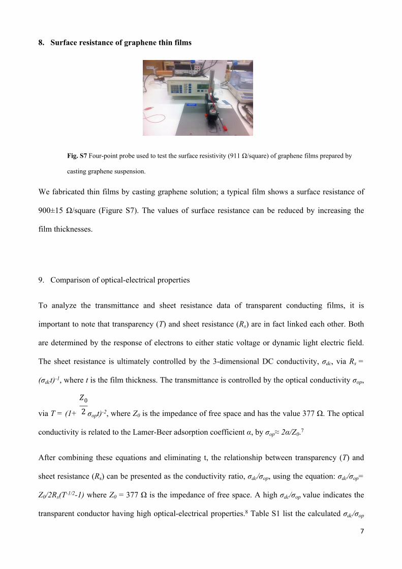
8. Surface resistance of graphene thin films

Fig. S7 Four-point probe used to test the surface resistivity (911 Ω/square) of graphene films prepared by

casting graphene suspension.

We fabricated thin films by casting graphene solution; a typical film shows a surface resistance of

900±15 Ω/square (Figure S7). The values of surface resistance can be reduced by increasing the

film thicknesses.

9. Comparison of optical-electrical properties

To analyze the transmittance and sheet resistance data of transparent conducting films, it is

important to note that transparency (T) and sheet resistance (Rs) are in fact linked each other. Both

are determined by the response of electrons to either static voltage or dynamic light electric field.

The sheet resistance is ultimately controlled by the 3-dimensional DC conductivity, σdc, via Rs =

(σdct)-1, where t is the film thickness. The transmittance is controlled by the optical conductivity σop,

via T = (1+ σopt)-2, where Z0 is the impedance of free space and has the value 377 Ω. The optical

𝑍02

conductivity is related to the Lamer-Beer adsorption coefficient α, by σop≈ 2α/Z0.7

After combining these equations and eliminating t, the relationship between transparency (T) and

sheet resistance (Rs) can be presented as the conductivity ratio, σdc/σop, using the equation: σdc/σop=

Z0/2Rs(T-1/2-1) where Z0 = 377 Ω is the impedance of free space. A high σdc/σop value indicates the

transparent conductor having high optical-electrical properties.8 Table S1 list the calculated σdc/σop

8

values for transparent conductors fabricated by various methods. In comparison, our transparent

graphene film could have better opt-electrical properties than other films made by (i) spin coating

and dip coating of reduced GO and (ii) electrochemically exfoliation of raw graphite.

Table S1 Comparison of our sheet film with previous ones.

FabricationMethods

Graphenetype

SheetResistance

(Ω/sq)

Transmittance(%)

σdc/σop Reference

Oxidi-sonication 815 86 2.95 Current work

Thermal reduction of GO 1000 80 1.60 [9]Spin coating

Thermal reduction of GO 2700 90 1.3 [10]

Thermal and Chemical

reduction of GO459 90 7.29 [8]

Chemical reduction

modified GO8000 83 0.24 [11]

Langmuir-Blodegett

Deposition

Chemical reduction of GO 1100 91 3.54 [12]

Vacuum filtration Chemical reduction of GO 350 80 4.5 [13]

Electrochemically exfoliation Graphene 2400 73 0.46 [14]

Dip coating Thermal reduction of GO 1800 70 0.54 [15]

Ni Substrate 1000 90 3.5 [16]

Ni Substrate 230 72 4.6 [17]CVD

Cu Substrate 350 90 9.96 [18]

9

10. Current–voltage characteristics of graphene films

a b

Fig. S8 Current–voltage measurement (a) devices and (b) characteristics

In Fig. S8, the current-voltage measurement indicates that the oxidi-sonication graphene films have

high conductivity.

Figure S9 shows an AFM image and its height profile of a graphene sheet made by the oxidi-

sonication of 60 min. The image is the same as in Figure 2d, but it measured the height of a

relatively large sheet. The height peak demonstrates both flat area and spikes; the latter is most

likely caused by either uneven sheet surface or AFM resolution.

Fig. S9 AFM image and its height profile for graphene sheets made by 60-min oxidi-sonication

10

References

1. D. C. Marcano, D. V. Kosynkin, J. M. Berlin, A. Sinitskii, Z. Sun, A. Slesarev, L. B. Alemany, W. Lu, J. M. Tour, ACS Nano, 2010, 4, 4806–4814.

2. A. M. Dimiev, L. B. Alemany, J. M. Tour, ACS Nano 2012, 7, 576–588.

3. B. Konkena, S. Vasudevan, J. Phys. Chem. Lett. 2012, 3, 867–872.

4. S. Dubin, S. Gilje, K. Wang, V. C. Tung, K. Cha, A. S. Hall, J. Farrar, R. Varshneya, Y. Yang, R. B. Kaner, ACS Nano, 2010, 4, 3845–3852.

5. C. Cheng, D. Li, Adv. Mater. 2013, 25, 13–29.

6. H. W. Kim, H. W. Yoon, S. M. Yoon, B. M. Yoo, B. K. Ahn, Y. H. Cho, H. J. Shin, H. Yang, U. Paik, S. Kwon, J. Y. Choi, H. B. Park, Science. 2013, 342, 91–95.

7. S. De, J. N. Coleman, ACS Nano, 2010, 4, 2713–2720.

8. Q. Zheng, W. H. Ip, X. Lin, N. Yousefi, K. K. Yeung, Z. Li, J. K. Kim, ACS Nano, 2011, 7, 6039–6051.

9. H. A. Becerril, J. Mao, Z. Liu, R. M. Stoltenberg, Z. Bao, Y. Chen, ACS Nano, 2008, 2, 463–470.

10. I. N. Kholmanov, S. H. Domingues, H. Chou, X. Wang, C. Tan, J. Y. Kim, H. Li, R. Piner, A. J. G. Zarbin, R. S. Ruoff. ACS Nano. 2013, 7, 1811–1816.

11. X. L. Li, G. Y. Zhang, X. D. Bai, X. M. Sun, X. R. Wang, E. Wang and H. J. Dai, Nat. Nanotechnol., 2008, 3, 538–542.

12. X. Lin, J. Jia, N. Youse, X. Shen and J. K. Kim, J. Mater. Chem. C, 2013, 1, 6869–6877.

13. H. Feng, R. Cheng, X. Zhao, X. Duan and J. Li, Nat. Commun., 2013, 4, 1539.

14. K. Parvez, R. Li, S. R. Puniredd, Y. Hernandez, F. Hinkel, S. Wang, X. Feng and K. Müllen, ACS Nano, 2013, 7, 3598–3606.

15. X. Wang, L. Zhi, K. M llen. Nano Lett., 2008, 8, 323–327.�̈�

16. A. Reina, X. Jia, J. Ho, D. Nezich, H. Son, V. Bululovic, M. S. Dresselhaus, J. Kong, Nano Lett., 2009, 9, 30–35.

17. L. G. D. Arco, Y. Zhang, C. W. Shlenker, K. Ryu, M. E. Thompson, C. Zhou, ACS Nano., 2010, 4, 2865–2873.

18. X. Li, Y. Zhu, W. Cai, M. Borysiak, B. Han, D. Chen, Richard. D. Piner, L. Colombo, R. S. Ruoff, Nano Lett., 2009, 9, 4359–4363.