Supply Chain Threats and Countermeasures: From Elicitation throughOptimization

Weihong “Grace” GuoRutgers University

wg152@soe.rutgers.edu

Paul KantorPaul B Kantor, Consultantpaulbkantor@gmail.com

Elsayed A. ElsayedRutgers University

elsayed@soe.rutgers.edu

Eric RosenbergGeorgian Court Universityerosenberg@georgian.edu

Rong LeiRutgers University

rl839@scarletmail.rutgers.edu

Sachin PatelRutgers University

sap357@scarletmail.rutgers.edu

Brendan RuskeyRutgers University

bjr110@scarletmail.rutgers.edu

Fred S. RobertsRutgers University

froberts@dimacs.rutgers.edu

Abstract

There are many checklists for improving supplychain resilience under different threats, but a lack ofconcrete procedures to rigorously assess and selectamong countermeasures (CMs). We present a novelprocess and method to elicit the needed informationto identify CMs and assess their ability to reducerisk. We report on the fine-grained analysis underlyingan effective simulation developed to model both theimpact of threats and the impact of alternative CMs inthe information and communication technology supplychain subject to disruptions due to natural hazards. Wealso describe the coarse-grained descriptions neededto elicit risk reduction estimates from subject matterexperts, and the problems of integrating these twoapproaches, bottom up, and top down, to supportmanagement decisions to choose an optimal set of CMsgiven a limited budget.

1. Introduction

1.1. Problem and Approach

Every nation is increasingly aware that informationand communication technologies are sourced fromaround the world, with the best performance costratios often coming from sources that are vulnerableto a number of threats. The information andcommunications technology (ICT) products andservices supply chain is vulnerable at every point fromthe design of chips to the moment that equipmentor software is installed. The U.S. is responding,particularly through the Department of HomelandSecurity (DHS) Cybersecurity and Infrastructure

Security Agency (CISA), and specifically CISA’sInformation and Communications Technology SupplyChain Risk Management Task Force Working Group2: Threat Evaluation. This group has identified ninecategories of threats to the ICT supply chain andhas developed specific threat scenarios for each threatcategory that are detailed enough to be useful to industryand government decision makers. The Working Group 2report [1] has served as a starting point for this project.

We report on a methodology to quantify the impact,measured by reduction in risk associated with specificcountermeasures (CMs) to threat scenarios. With thehelp of CISA and industry experts from a projectAdvisory Board, we have selected and specified threethreat scenarios that span many kinds of issues thatare representative of the major issues raised in theWorking Group 2 report and from which our workshould be readily generalizable to the other threats ofinterest. The first involves natural hazards: floods,storms, earthquakes. They are modeled at the levelof plants and interconnections. The second scenarioinvolves counterfeit materials. They are modeledby a flow of individual parts or components. Thethird scenario involves problems of “onboarding” anew supplier. This represents problems of financialstability, technical competence, intellectual propertyrights, and geopolitical factors. Our methodology hasthree components: elicitation of CMs and risk reductionestimates from subject matter experts (SMEs), networkmodeling and simulation of the supply chain, and useof optimization tools to choose an optimal set of CMs.We report on application of our methods to the naturalhazards threat. While our methodology can be easilyextended to the other two threats we have studied, thetechnical details, such as changing from a plant-based

simulation to an agent-based model for parts requiresdetailed expansion of the description that is beyond thescope of a short paper.

We gather input from SMEs in a Zoom-basedfocus group approach that includes development ofconsensus risk reduction estimates. From theseconsensus estimates, sophisticated computer simulationusing the anyLogistix tool [2] generates hundredsof random examples. This “Monte Carlo” methodis the gold standard for uncertainty in finance andclimate. To identify best decisions, simulationsare tied to an optimization algorithm using MixedInteger Programming that considers many possiblecombinations of protections. For any given budget itfinds the best allocation of limited funds.

This project is developing a methodology that wehope will be of use to CISA, other components of DHS,and the private sector. Our tools provide new approachesto eliciting expert assessments of relative risk reductionof different CMS. Our network models and simulationsfor supply chains and our optimization models forselecting the most effective set of CMs should be ofinterest to those concerned with understanding the riskreduction of different mitigation strategies for supplychain disruptions. The results should provide someinsight about supply chain threats such as those in thethree chosen scenarios, but also more generally to a widevariety of scenarios and to a wide variety of types ofsupply chains, not just for ICT.

The elicitation process, network modeling andsimulations of supply chains, and optimization toolsboth inform and are informed by each other. Section2 describes the elicitation procedure. The details of thenetwork models are presented in Section 3, while theapproach we have developed for optimization appears inSection 4. We discuss the challenges of integrating thesethree project components into a single coherent toolfor planning and decision making, and some possibleextensions of this work, in Section 5.

1.2. Related Literature

This project has benefited from an extensiveliterature on supply chains and supply chain resiliency;elicitation of risk and risk reduction; modeling andsimulation; and approaches to risk and risk reductionin the three scenarios of interest. We mention selectedwork that has influenced our own approach.

Supply Chains/Scenarios/Threats: Recentrelevant supply chain risk/disruption reviews arepresented in [3] and [4]. An earlier work that usedextensive qualitative methods is in [5]. However, theliterature lacks information on the quantitative impact

of specific mitigations and CMs.The key source for our selection of threats/scenarios

is the analysis of CISA Working Group 2 [1]. Thereis also an enormous literature on CMs. This literatureproposes checklists, often with anecdotal evidence aboutsome mitigation, leaving users to select their ownportfolios for implementation. We have found that theliterature on threats to supply chains under the threescenarios of interest was the most helpful part of thesupply chain literature, so we describe it here.

Natural Disasters: Public sources such as [6] andreports from FEMA (Federal Emergency ManagementAgency), ASCE (American Society of Civil Engineers),and NOAA (National Oceanographic and AtmosphericAdministration) provide useful information regardingmultiple hazards. Data analytic approaches such asthose of [7, 8, 9, 10] have been very helpful inproviding ways to quantify and characterize supplychain resilience under multiple natural hazards, helpingus develop performance metrics for our simulations.

Counterfeit Parts: The presence of counterfeitproducts has led to the development of the SuspectCounterfeit database in GIDEP (Government-IndustryData Exchange Program) [11], a very helpful resource.The Electronic Resellers Association (ERAI) is amajor resource with the world’s largest databaseof suspect counterfeit and noncomforming electronicparts [12]. The literature also describes bestpractices for government and industry, e.g., theNavy’s Counterfeit Materiel Process Guidebook [13]provides tools for implementing a risk-based counterfeitmateriel prevention program such as ours. [14]provides counterfeit risk mitigation strategies and[15] describes challenges of increasing reliance oncommercial-off-the-shelf (COTS) components. Webuild on similar strategies, e.g., different inspectionprocedures for components from selected vendors orfrom COTS sources. [16] suggests using different kindsof tests; likewise, our simulations allow for differentlevels of testing based on questionable behavior.[17] suggests stronger preventive measures, whichare reflected in our simulations studying pre-event orpreventive CMs as well as post-event CMs. [18]describes what makes a good counterfeit prevention planand [19] lays out a prototype agent-based simulation thatimplements an anti-counterfeiting framework. As in ourproject, the goal is to use such simulations to identifyeffective anti-counterfeiting policies. However, no priorwork similar to our approaches has been reported in theliterature.

Onboarding of New Suppliers: The literaturelacks quantitative metrics or simulation modeling ofthe onboarding of new suppliers. The CISA Working

Group 2 description of an onboarding threat scenarioemphasizes financial health and early warning signs thata vendor might be dependent on a foreign governmentfor financial support, signs also mentioned in thedescription of MITRE’s Supply Chain Security Systemof Trust [20]. The literature on counterfeit parts isrelevant to the onboarding threat as well. For example,[17] recommends that a vendor’s reporting of counterfeitparts be monitored and failures potentially leadingto debarring, ideas our models and simulations use.Digital watermarking of physical and digital documents(and components) is among the CMs relevant to theonboarding scenario, with publications such as [21, 22,23, 24] influencing our work.

Elicitation: There are many reviews of the literatureon elicitation, e.g., [25]. When scientific advice isused in government decision making, the traditionalapproach has been committee discussion, which canresult in bias. This was one motivation for developmentof more structured decision-making processes suchas Delphi [26, 27]. Formal procedures for elicitingjudgments about risk and risk reduction from experts,and pooling their judgments, can help to quantify riskas well as uncertainty [28]. We started with establishedprocedures for eliciting estimates of risk (e.g., [27]).After reviewing many methods, such as those reviewedin [25] and the ones instantiated in [29] and [30], weadopted a recent method aimed at experts unfamiliarwith probabilities [31]. This method extends the classicmethods for the combination of probabilities initiated in[32]. The central idea is that distributions need not bewell modeled by a well-behaved ”Bayesian conjugatedistribution,” since all down-stream calculations arenumerical Monte Carlo simulations. [30] presented asimilar idea, although their conceptual framework seeksa parametric form for the distribution. Our elicitationuses extensions of classical methods by [33, 34, 35, 36].[35] and [36] point out the importance of trainingexperts in making probability judgments, influencing usto include a training component in our elicitation. In ourfocus groups estimates are aggregated by averaging, assuggested by [32], and also using a generalization of themedian concept given by [37].

Our approaches to elicitation of risk and riskreduction are grounded in the large literature on riskmanagement. [38] and [39] present the process ofrisk management in steps: risk identification, riskassessment, risk mitigation, and situation monitoring.Our work concentrates on the risk assessment and riskmitigation steps – with an emphasis on identifying CMsto reduce risk. [40] points out how to extend thisstepwise model to the notion of opportunity, the idea thatevents can also provide positive impacts, which we do

not consider. [41] describes risk as the combination ofthe severity of the effects and probability of occurrence.This reflects the fact that performance of a supply chainis dependent on changing conditions, some of which(such as occurrence and severity of a natural disaster)are beyond our ability to measure – and something ourelicitation processes and our simulation models reflect.Risk reduction occurs in the context of uncertainty. [40]has proposed an interesting framework that reflects thereality that no supply chain will have a static stableequilibrium in a world with a constantly changingenvironment. Our work also builds on the dynamicnature of supply chains and the idea that risk and riskreduction are dynamic concepts.

Simulation: Simulation allows us to study complex,real-world systems with stochastic elements and to“see” how different scenarios of disruptions andimplementations of CMs impact the entire supplychain. Simulation has been widely used fortackling the uncertainties in supply chain networks.[42] reviewed several simulation techniques thatquantitatively addresses uncertainty in supply chains.[43] developed a framework of a digital supply chaintwin for managing the risks in pre, during, and postdisruption stages. [44] proposed a dynamic modelfor evaluating the service level of supply chains inscenarios with disruptions. Mathematical formulationof the network is difficult since the causes of disruptionsand their severities are often random with unknownprobability distributions, so a simulation model of thenetwork is a viable and realistic approach to evaluatethe dynamic performance of supply chain(s) in virtualenvironments [45, 46, 47].

Our simulation models include estimates of boththe degradation rate and recovery rate in modeling theability of each node and arc to meet performance levels.These are combined to quantify overall supply chainperformance. We compute importance measures foreach node or arc, extending the importance measuresdiscussed in [48] to incorporate multiple threat types.

2. Elicitation

Subject Matter Experts (so far 34 interviewed, 18also in Focus Groups) are recruited in a “snowball”process, starting with members of the project AdvisoryBoard. Each is interviewed, and those with specificexperience in the effectiveness of mitigations are invitedto a Zoom-based focus group process, supported by anew FGWare algorithm. After discussion to select ahandful of CMs, each SME provides estimates of howmuch each specific mitigation reduces risk. We combinethese estimates to form a consensus. We operationalize

“amount of risk reduction” based on Eq. 1, familiarthroughout the field of risk management. The amountof risk reduction corresponds to the variable denoted byE in Eq. 2

R0 = Consequences ∗Vulnerability ∗ Threat (1)Reduced Risk = (1−E) ∗R0 (2)

We sketch the approach to two technical issues,detailed in [49].

To elicit probability distributions, as discussed inSection 1.2, we use a recent method aimed at expertsunfamiliar with probabilities [50].

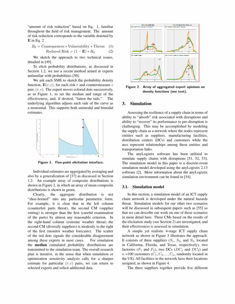
We ask each SME to sketch the probability densityfunction, E(r, c), for each risk r and countermeasure cpair, (r, c). The expert moves colored dots successively,as in Figure 1, to set the median and range of theeffectiveness, and, if desired, “fatten the tails.” Theunderlying algorithm adjusts each side of the curve asa monomial. This supports both unimodal and bimodalestimates.

Figure 1. Five-point elicitation interface.

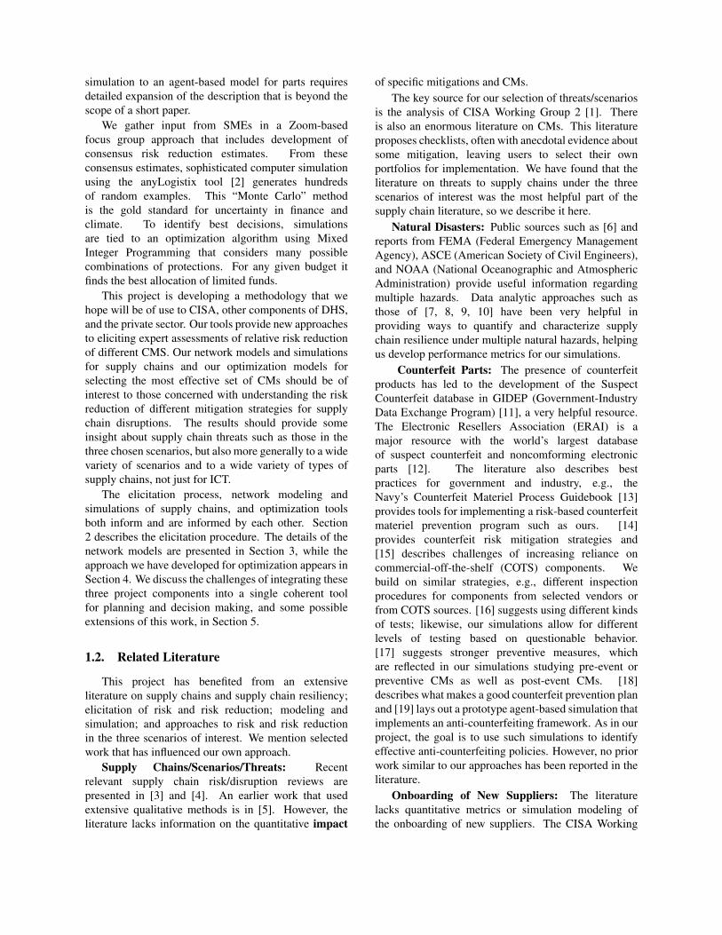
Individual estimates are aggregated by averaging andalso by a generalization of [37] as discussed in Section1.2. An example array of composite distributions isshown in Figure 2, in which an array of mean compositedistributions is shown in green.

Clearly, the aggregate distribution is not“shoe-horned” into any particular parametric form.For example, it is clear that in the left column(counterfeit parts threat), the second CM (suppliervetting) is stronger than the first (careful examinationof the parts) by almost any reasonable criterion. Inthe right-hand column (extreme weather threat) thesecond CM (diversify suppliers) is modestly to the rightof the first (monitor weather forecasts). The scatterof the red dots signals the considerable disagreementamong these experts in most cases. For simulationthe median cumulated probability distributions aretransmitted to the simulation team. The overall researchplan is iterative, in the sense that when simulation oroptimization sensitivity analysis calls for a sharperestimate for particular (r, c) pairs, we can return toselected experts and solicit additional data.

Figure 2. Array of aggregated expert opinions on

density functions (see text).

3. Simulation

Assessing the resilience of a supply chain in terms ofability to “absorb” risk associated with disruptions andability to “recover” its performance to pre-disruption ischallenging. This may be accomplished by modelingthe supply chain as a network where the nodes represententities such as suppliers, manufacturing facilities,distribution centers (DCs) and customers while thearcs represent relationships among these entities andtransportation links.

The anyLogistix software has been utilized tosimulate supply chains with disruptions [51, 52, 53].The simulation model in this paper is a discrete-eventsimulation model developed using the anyLogistix 2.13software [2]. More information about the anyLogistixsimulation environment can be found in [54].

3.1. Simulation model

In this section, a simulation model of an ICT supplychain network is developed under the natural hazardsthreat. Simulation models for our other two scenarioswill be discussed in subsequent papers such as [55] sothat we can describe our work on one of these scenariosin more detail here. Three CMs based on the results ofthe elicitation study (see Section 2) are investigated, andtheir effectiveness is assessed in simulation.

A simple yet realistic 4-stage ICT supply chainnetwork as shown in Figure 3 illustrates the approach.It consists of three suppliers (S1, S2, and S3, locatedin California, Florida, and Texas, respectively), twofactories (F1 and F2), two DCs (DC1 and DC2) andn =100 customers (C1, C2, ..., Cn, randomly located inthe US). All facilities in the network have their locationsassigned, as shown in Figure 4.

The three suppliers together provide five different

Figure 3. Supply chain network.

Figure 4. Simulated network of ICT supply chain.

components (screen, keyboard, motherboard, battery,and laptop base) to the factories. Factories assemble thecomponents into laptops. Finished laptops are deliveredto DCs and then customers.

3.1.1. Baseline scenario

In our baseline scenario, there are no disruptions tothe supply chain, and its performance level is 100%(meeting all requested demand on time). Each of thefive components is shipped from a supplier to a factoryaccording to a pre-specified ratio. A factory may receivea type of component from one or more suppliers: S1

provides a proportion p1 of its demand, and similarlyfor S2 and S3. The values of (p1, p2, p3) are shown inTable 1. For example, both factories receive all of theirscreens from S1. F2 receives 1/3 of the keyboards fromS1 and the remaining 2/3 from S2. The transportationbetween a supplier and a factory takes 5 hours.

Table 1. Sourcing table showing proportions of

components from each supplier to each factory.(p1, p2, p3) F1 F2

Screen (1, 0, 0) (1, 0, 0)Keyboard (0.5, 0.5, 0) (0.333, 0.667, 0)Motherboard (0, 0.625, 0.375) (0, 0.333, 0.667)Battery (0, 1, 0) (0, 0.167, 0.833)Laptop base (0, 0, 1) (0, 0, 1)

Factories use the QR inventory policy (fixedreplenishment quantity policy) with (Q,R) = (1000,600), starting laptop inventory at s = 1500 units, andcomponent inventory at r = 1000 units for each type.The throughput is p = 150 units/day at each factory.

Each factory provides proportions of the demand to theDCs. DC1’s demand is fulfilled by F1 and F2 equally,while 40% of DC2’s demand is fulfilled by F1 and60% by F2. The total factory demand is based on therequested demand from customers to the DCs. Thetransportation between a factory and a DC takes 5 hours.

DCs also use the QR policy with (Q,R) = (1000,600) and starting inventory at s = 1500 units. Each of thecustomers places a demand every single day accordingto a uniform distribution of U(1, 3) units. The demand issent to the closest DC. Based on the network in Figure4, there are 45 customers sending orders to DC1, and55 customers to DC2, every day. The transportationbetween a DC and a customer takes 3 days.

3.1.2. Threat scenario

In the threat scenario, natural hazards occur butno CMs are introduced. Factories F1 and F2 arelocated in an area subject to earthquakes and hurricanesrespectively. When a natural hazard occurs, it willshut down the factory in the area for a number ofdays. The frequency of earthquakes/hurricanes and theirseverities are expressed by random variables based onthe historical data of the area. The risk associated withthe severity is the duration of the disruption, which isexaggerated from reality to better show the impact of thethreat. Table 2 shows the parameters in this scenario.

Table 2. Model parameters in the threat scenario.Natural hazard Earthquake HurricaneFacility impacted F1 F2

Frequency Once during Jun-NovStarting date RandomDuration (day) 60 w.p. 0.5, 90 w.p. 0.3, 120 w.p. 0.2

3.1.3. Countermeasure scenarios

Three different CMs (CM1, CM2, and CM3) havebeen developed to provide resilience during disruptiveevents caused by natural hazards. CM1 and CM2are reactive CMs that are implemented after the actualoccurrence of the event. CM3 is a proactive CMdesigned for pre-disruption implementation.

When a factory is shut down due to a naturalhazard, we can increase the throughput of the remainingoperating factory to help meet the demand, but thisincrease takes several days to implement. So, in CM1,we increase the throughput of the remaining factorya few days after the disruption, and the throughputremains increased till the end of the disruption.

In CM2, we introduce an outsourcing factory tohelp cope with the demand. This outsourcing factorymay be reconfigured and subcontracted to handle laptop

assembly, which takes several days. Since this factory islocated in a non-impacted area, transportation betweenit and DCs takes longer.

Pre-disruption CM3 uses accurate monitoringsystems for potential natural hazards, based on whichearly actions can be planned in advance. In the daysleading to the disruption, we can increase the throughputof the to-be-impacted factory so that more laptops canbe assembled before the event. The inventory policiesof the DCs are adjusted accordingly so more finishedlaptops are delivered to DCs before the event.

Table 3 summarizes all five scenarios and theparameters in the three Threat + CM scenarios.

Table 3. Scenario description and parameters.Scenario DescriptionBaseline Normal operation, no disruption.Threat Natural hazards occur but no CMs are introduced.Threat+ CM1

Ten days after disruption, the remaining operatingfactory’s throughput increases to 200 units/day.

Threat+ CM2

Ten days after disruption, an outsourcing factorybecomes operational, but transportation from theoutsourcing factory to DCs takes 10 days.

Threat+ CM3

During the 15 days leading to disruption, factory’sthroughput increases to 200 units/day, and DC’sreorder point increases to 900 units.

3.1.4. Performance metrics

Five performance metrics are computed to evaluatethe performance of the supply chain and effectivenessof the CMs.

(1) ELT Service Level by Orders shows the servicelevel based on the ratio of on time orders to the overallnumber of outgoing orders:

ELTSL(i) = OTO/(OTO +DO) (3)

where i is the facility index, OTO is the number of ontime orders, and DO is the number of delayed orders.OTO+DO is the number of outgoing orders. The ELT(expected lead time) is set at 4 days, allowing 3 daysfor transportation and 1 day for order processing. Anon time order is one for which the time from customerorder placement to delivery is within the ELT.

(2) Service Level by Orders shows the service levelbased on the ratio of the number of successfully fulfilledorders to the sum of all orders placed for this facility:

SL(i) = SO/(SO + UO) (4)

where i is the facility index, SO is the number of ordersthat are successfully fulfilled, and UO is the number ofunsuccessful orders. Unsuccessful orders are the placedorders requiring the quantity of products that is notavailable at the facility at the time of order placement.

(3) Max Lead Time is the maximum time betweenorder placement and delivery across all orders.

(4) Mean Lead Time is the average time betweenorder placement and delivery across all orders.

(5) Fulfillment (Late Products) shows the quantityof product which fails to arrive within the specified ELT.

3.2. Results and comparison

We use feedback from stakeholders (industryAdvisory Board and DHS) throughout network modeldesign and simulation to verify the work by usingsmall-size, deterministic demand and following itthrough the network using “manual” calculations. Afterthe verification process, the demand is increased andmore stochasticity added, and we simulate for oneyear to observe enough inventory cycles and stockoutsituations, with 30 replications per scenario. Thenumber of replications is chosen for the Central LimitTheorem to hold. The 30 replications take about 60seconds on a Windows 2017 computer (Intel Core i7).Model validation is achieved by discussing the outputwith the stakeholders, but true validation will only bepossible when/if the model is used by government orindustry in specific situations.

The ELT service level by orders and service levelby orders are recorded for each day in the simulation.The daily values are then averaged over the threat periodwithin each replication. Table 4 shows the “threat periodaverage” values across 30 replications. A service levelcloser to 1 indicates a more resilient supply chain. Ascan be seen, both metrics are severely affected whenno CMs are employed. All 3 CMs improve upon thethreat scenario. CM2 is the least effective one, becauseit is enacted 10 days after the threat has occurred andthe transportation time from the outsourcing factory is7 days more than usual. This is why the ELT servicelevel is still poor. CM1 is ranked second. This CM isalso enacted 10 days after the threat has occurred but theproduction speed of the remaining factory is increasedwith no extra transportation time. CM3 is the mosteffective CM due to the 15-day early actions obtainedand the increased inventory levels and production speedsto deal with the threat.

Table 4. Average service levels from simulation.ELT Service Level Service Level

Scenario DC1 DC2 DC1 DC2

Threat only 0.3762 0.3678 0.3276 0.3292Threat + CM1 0.9616 0.9272 0.9675 0.9549Threat + CM2 0.8089 0.7947 0.7917 0.7668Threat + CM3 0.9985 0.9955 0.9970 0.9944

The max lead time and mean lead time performancemetrics are summarized in Table 5, showing the average

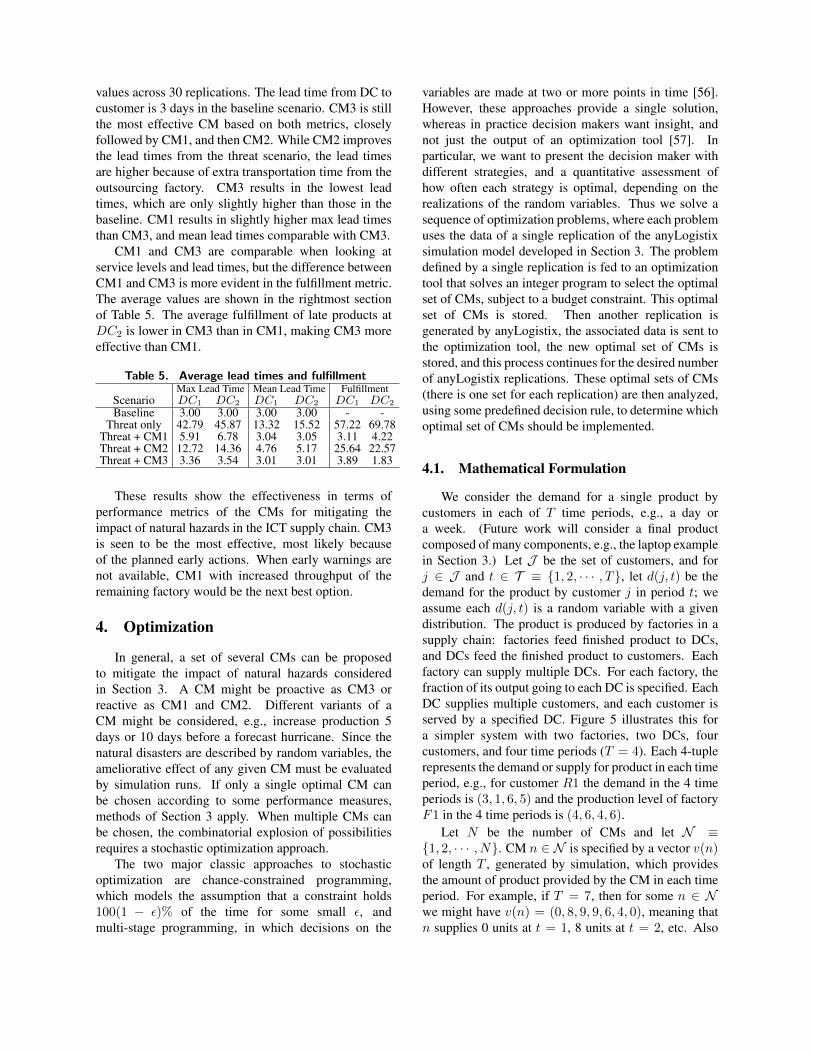
values across 30 replications. The lead time from DC tocustomer is 3 days in the baseline scenario. CM3 is stillthe most effective CM based on both metrics, closelyfollowed by CM1, and then CM2. While CM2 improvesthe lead times from the threat scenario, the lead timesare higher because of extra transportation time from theoutsourcing factory. CM3 results in the lowest leadtimes, which are only slightly higher than those in thebaseline. CM1 results in slightly higher max lead timesthan CM3, and mean lead times comparable with CM3.

CM1 and CM3 are comparable when looking atservice levels and lead times, but the difference betweenCM1 and CM3 is more evident in the fulfillment metric.The average values are shown in the rightmost sectionof Table 5. The average fulfillment of late products atDC2 is lower in CM3 than in CM1, making CM3 moreeffective than CM1.

Table 5. Average lead times and fulfillmentMax Lead Time Mean Lead Time Fulfillment

Scenario DC1 DC2 DC1 DC2 DC1 DC2

Baseline 3.00 3.00 3.00 3.00 - -Threat only 42.79 45.87 13.32 15.52 57.22 69.78

Threat + CM1 5.91 6.78 3.04 3.05 3.11 4.22Threat + CM2 12.72 14.36 4.76 5.17 25.64 22.57Threat + CM3 3.36 3.54 3.01 3.01 3.89 1.83

These results show the effectiveness in terms ofperformance metrics of the CMs for mitigating theimpact of natural hazards in the ICT supply chain. CM3is seen to be the most effective, most likely becauseof the planned early actions. When early warnings arenot available, CM1 with increased throughput of theremaining factory would be the next best option.

4. Optimization

In general, a set of several CMs can be proposedto mitigate the impact of natural hazards consideredin Section 3. A CM might be proactive as CM3 orreactive as CM1 and CM2. Different variants of aCM might be considered, e.g., increase production 5days or 10 days before a forecast hurricane. Since thenatural disasters are described by random variables, theameliorative effect of any given CM must be evaluatedby simulation runs. If only a single optimal CM canbe chosen according to some performance measures,methods of Section 3 apply. When multiple CMs canbe chosen, the combinatorial explosion of possibilitiesrequires a stochastic optimization approach.

The two major classic approaches to stochasticoptimization are chance-constrained programming,which models the assumption that a constraint holds100(1 − ε)% of the time for some small ε, andmulti-stage programming, in which decisions on the

variables are made at two or more points in time [56].However, these approaches provide a single solution,whereas in practice decision makers want insight, andnot just the output of an optimization tool [57]. Inparticular, we want to present the decision maker withdifferent strategies, and a quantitative assessment ofhow often each strategy is optimal, depending on therealizations of the random variables. Thus we solve asequence of optimization problems, where each problemuses the data of a single replication of the anyLogistixsimulation model developed in Section 3. The problemdefined by a single replication is fed to an optimizationtool that solves an integer program to select the optimalset of CMs, subject to a budget constraint. This optimalset of CMs is stored. Then another replication isgenerated by anyLogistix, the associated data is sent tothe optimization tool, the new optimal set of CMs isstored, and this process continues for the desired numberof anyLogistix replications. These optimal sets of CMs(there is one set for each replication) are then analyzed,using some predefined decision rule, to determine whichoptimal set of CMs should be implemented.

4.1. Mathematical Formulation

We consider the demand for a single product bycustomers in each of T time periods, e.g., a day ora week. (Future work will consider a final productcomposed of many components, e.g., the laptop examplein Section 3.) Let J be the set of customers, and forj ∈ J and t ∈ T ≡ {1, 2, · · · , T}, let d(j, t) be thedemand for the product by customer j in period t; weassume each d(j, t) is a random variable with a givendistribution. The product is produced by factories in asupply chain: factories feed finished product to DCs,and DCs feed the finished product to customers. Eachfactory can supply multiple DCs. For each factory, thefraction of its output going to each DC is specified. EachDC supplies multiple customers, and each customer isserved by a specified DC. Figure 5 illustrates this fora simpler system with two factories, two DCs, fourcustomers, and four time periods (T = 4). Each 4-tuplerepresents the demand or supply for product in each timeperiod, e.g., for customer R1 the demand in the 4 timeperiods is (3, 1, 6, 5) and the production level of factoryF1 in the 4 time periods is (4, 6, 4, 6).

Let N be the number of CMs and let N ≡{1, 2, · · · , N}. CM n ∈ N is specified by a vector v(n)of length T , generated by simulation, which providesthe amount of product provided by the CM in each timeperiod. For example, if T = 7, then for some n ∈ Nwe might have v(n) = (0, 8, 9, 9, 6, 4, 0), meaning thatn supplies 0 units at t = 1, 8 units at t = 2, etc. Also

Figure 5. Example supply chain with T = 4.

associated with n is a cost cost(n) e.g., a fixed cost ofopening an emergency assembly site plus an incrementalcost for each unit produced at the site over the T timeperiods. For n ∈ N , let the binary variable x(n) bedefined by x(n) = 1 if CM n is implemented, andx(n) = 0 otherwise. A budget B limits the total cost ofCMs:

∑n∈N cost(n)x(n) ≤ B . Each factory sends its

output to one or more DCs, and the fraction of the outputof a given factory to the set of DCs is given data. SinceCMs offset the loss in production capacity at a specificfactory when disasters occur, the output of each CM isallocated to the set of DCs using these same fractionalallocations. Let DC be the set of DCs.

If a threat materializes, and the factories are unableto ship sufficient products to meet the demand for oneor more customers, demand is backlogged rather thanlost. The objective is to minimize the total (over all timeperiods and customers) backlogged demand. Since eachcustomer is served by a particular DC i, for each timeperiod t we can sum (over all customers) the demand tobe served by DC i; let d(i, t) be this aggregate demandat DC i in period t. Let s(i, t) be the amount of productsupplied to DC i at time t given the current replication.For example, if the replication has no threat occurring,then s(i, t) is the amount supplied to DC i undernormal operating conditions, while if the replication hasreduced production at one or more factories, then s(i, t)reflects the reduced product available at DC i at timeperiod t if no CM is implemented. For a given t theamount of backlogged demand at DC i if no CM isimplemented is max{d(i, t)− s(i, t), 0}.

For n ∈ N and i ∈ DC and t ∈ T , let b(n, i, t)be the given data specifying the amount of productprovided at time t to DC i if CM n is implemented. IfCM n does not back up DC i then b(n, i, t) = 0. Thenthe total threat mitigation supply sent by all CMs toDC i in time t is

∑n∈N b(n, i, t)x(n), the total amount

L(i, t) of product backlogged at DC i at time t is

L(i, t) ≡ max{d(i, t)− s(i, t)−

∑n∈N

b(n, i, t)x(n), 0}

and the total amount of product backlogged over all DCsand over all time periods is the objective function F (x):

F (x) ≡∑t∈T

∑i∈DC

L(i, t) .

Using standard techniques for dealing with a “max”term, F (x) can be converted to a linear objectivefunction together with associated constraints. ThePython PuLP package [58], using the COIN-OR CBCsolver [59], solves the optimization problem. Thesolution to this optimization problem (correspondingto a particular simulation replication) is stored, andanother simulation replication is generated. Togetherthey support calculations of the mean impact and othermeasures of risk and resilience.

The results of the optimization expand upon theconclusions in Section 3 that CM3 is the most effectiveCM, followed by CM1, and then CM2. With 100replications and B = 1, CM3 at factory 1 (F1) is chosen69 times, and CM3 at F1 is chosen 31 times. With 100replications and B = 2, CM3 at both F1 and F2 ischosen 100 times. We also studied a larger example,with 8 factories, 6 distribution centers, 100 customers,and B = 2. With 100 replications, 18 distinct sets ofCMs were generated; the most frequent set generated(25 replications) used CM3 at F2 and F4; the next mostfrequent set (19 replications) used CM3 at F2 and F3.

5. Discussion

This work models an end-to-end approach thatrecognizes the fundamentally stochastic nature of riskmitigation and resilience. By developing the threecomponents of elicitation, simulation, and optimizationwe are able to inform each component by the specificand changing needs of the other two, which brings uscloser to the goal of providing a sound quantitativemethodology for making rational decisions under alimited budget for risk mitigation.

If either simulation or optimization should revealthat the conclusions are particularly sensitive to thedetails of a distribution describing some risk-mitigationCM, SMEs could be reconvened to look for a resolution.

The integrated approach presented here offersspecific operationalizations of the concepts ofuncertainty about the effectiveness of mitigations,and the stochastic nature of all threats. The frameworkpermits comparison of CMs not solely in terms ofcosts, but also in terms of their likely ability to controlassociated risks. With suitable choices of the objectivesand performance metrics, this technology can beadapted for use at a single plant, a multi-locationorganization, or a state or federal agency.

There are numerous opportunities to enhance theoptimization model described in Section 4. The softwarecould accept a CM scenario and automatically generatevariations of it, or could be enhanced to considerthe impact of the QR inventory policies described inSection 3.1.1 or to allow any of the performance metricsdescribed in Section 3.1.4 to be used as the objectivefunction of the optimization.

Crucial information on effectiveness of specific CMsis gained in painful experience such as business setbackor failures. Organizations are unwilling to share suchinformation; even when resilience is achieved, thatfact may well be regarded as a proprietary advantage.A somewhat similar problem exists in the airlineindustry. However, over the years the commercialairlines and the Federal Aviation Administration havedeveloped a secure and trusted system for reportingnot only accidents, but also the much more common“near misses.” This work contributes toward a similartrust and benefit for the ICT supply chain. By asystematic integration of elicitation, simulation, andoptimization, our work provides a unified frameworkto assess CM effectiveness, strengthen resilience, andsupport planning and decision-making.

6. Acknowledgments

Acknowledgement: This material is basedupon work supported by the U.S. Department ofHomeland Security under Grant Award Number17STQAC00001-05-00. Disclaimer: The views andconclusions contained in this document are those of theauthors and should not be interpreted as necessarilyrepresenting the official policies, either expressed orimplied, of the U.S. Department of Homeland Security.The authors thank Niles Egan and Vladimir Menkov forconstruction of the 5-point elicitation tool.

References[1] CISA Working Group 2, “INFORMATION AND

COMMUNICATIONS TECHNOLOGY SUPPLYCHAIN RISK MANAGEMENT TASK FORCEThreat Evaluation Working Group: Threat ScenariosVersion 2.0.” https://www.cisa.gov/sites/default/files/publications/ict-scrm-task-force-threat-scenarios-report-v2.pdf, 2021.

[2] The AnyLogic Company, “anyLogistix supplychain optimization software.” https://www.anylogistix.com, 2021.

[3] K. Katsaliaki, P. Galetsi, and S. Kumar, “Supply chaindisruptions and resilience: a major review and futureresearch agenda,” Ann. Oper. Res., pp. 1–38, 2021.

[4] B. Fahimnia, C. S. Tang, H. Davarzani, and J. Sarkis,“Quantitative models for managing supply chain risks:A review,” Eur. J. Oper. Res., vol. 247, pp. 1–15, 2015.

[5] C. W. Craighead, J. Blackhurst, M. J. Rungtusanatham,and R. B. Handfield, “The severity of supply chaindisruptions: design characteristics and mitigationcapabilities,” Decision Sci., vol. 38, pp. 131–156, 2007.

[6] Centre for Research on the Epidemiology of Disasters,“EM-DAT: The International Disaster Database.”https://www.emdat.be/.

[7] D. Gama Dessavre, J. E. Ramirez-Marquez, andK. Barker, “Multidimensional approach to complexsystem resilience analysis,” Reliab. Eng. Syst. Safe.,vol. 149, no. C, pp. 34–43, 2016.

[8] Y. Li and C. W. Zobel, “Exploring supply chain networkresilience in the presence of the ripple effect,” Int. J.Prod. Econ., vol. 228, p. 107693, 2020.

[9] M. Ouyang and L. Duenas Osorio, “Time-dependentresilience assessment and improvement of urbaninfrastructure systems,” Chaos, vol. 22, p. 033122, 2012.

[10] C. Zobel and L. Khamsa, “Characterizing multi-eventdisaster resilience,” Comput. Oper. Res., vol. 42,pp. 83–94, 2014.

[11] GIDEP, “About GIDEP.” https://www.gidep.org/about/about.htm.

[12] ERAI, “About ERAI, Inc..” https://www.erai.com/aboutus_profile.

[13] Counterfeit Material Process Guidebook: Guidelinesfor Mitigating the Risk of Counterfeit Materiel inthe Supply Chain. NAVSO P-7000: Office of theAssistant Secretary of the Navy (Research, Development& Acquisition) Acquisition and Business Management,2017-06.

[14] S. Wix and D. Mahadeo, “Suspect/counterfeit electronicsoverview,” Component & System Analysis, 2017-05-11.

[15] A. R. Szakal and K. J. Pearsall, “Open industry standardsfor mitigating risks to global supply chains,” IBM J. RES.& DEV, vol. 58, no. 1, p. 1:1–13.

[16] C. Metz, Counterfeit Items Detection and Prevention.DLA J-334,: Defense Logistics Agency, America’sCombat Logistics Support Agency, 2012-09.

[17] J. S. Gansler, W. Lucyshyn, and J. Rigilano,Addressing counterfeit parts in the DOD supplychain. UMD-LM-14-012: Center for Public Policy andPrivate Enterprise, School of Public Policy, Universityof Maryland, 2014-03.

[18] Lockheed Martin, “Counterfeit prevention: What makesa good control plan?.” https://slidetodoc.com/counterfeit-prevention-what-makes-a-good-control-plan/.

[19] D. A. Bodner, “Enterprise modeling frameworkfor counterfeit parts in defense systems,” ProcediaComputer Science, vol. 36, pp. 425–431.

[20] R. A. Martin, “Trusting our supply chains: Acomprehensive data-driven approach,” tech. rep., MITRECenter for Data-Driven Policy, 2021-01 https://www.mitre.org/sites/default/files/publications/pr-20-01465-37-trusting-our-supply-chains-a-comprehensive-data-driven-approach.pdf.

[21] DARPA, “A DARPA approach to trustedmicroelectronics.” https://www.darpa.mil/attachments/Obscurationandmarking_Summary.pdf.

[22] R. Lingle, “In-mold labels use digital watermarking forauthentication,” Packing Digest, 2014-11-26, https://www.packagingdigest.com/trends-issues/mold-labels-use-digital-watermarking-authentication.

[23] Digital Watermarking Alliance, “Authentication ofcontent and objects (includes government ids).” https://digitalwatermarkingalliance.org/digital-watermarking-applications/authentication-of-content-and-objects/.

[24] CDC, “Tamper-resistant prescription formrequirements.” https://www.cdc.gov/phlp/docs/menu-prescriptionform.pdf.

[25] M. Chen, F. Brun, M. Raynal, C. Debord, andD. Makowski, “Use of probabilistic expert elicitation forassessing risk of appearance of grape downy mildew,”Crop Protection, vol. 126, p. 104926, Dec. 2019.

[26] N. C. Dalkey, “The Delphi Method: An experimentalstudy of group opinion,” RAND Corporation ReportRM-5888-PR, 1969.

[27] H. A. Linstone and M. Turoff, eds., The Delphi Method:Techniques and Application. Reading, MA: AddisonWesley, 1975.

[28] W. P. Aspinall and R. M. Cooke, “Quantifying scientificuncertainty from expert judgement elicitation,” inRisk and Uncertainty Assessment for Natural Hazards(J. Rougier, S. Sparks, and L. Hill, eds.), CambridgeUniversity Press, 2013.

[29] S. Mitchell and I. Dunning, “MATCH Elicitation tool.”http://optics.eee.nottingham.ac.uk/match/uncertainty.php#, 2021.

[30] D. E. Morris, J. E. Oakley, and J. A. Crowe, “Aweb-based tool for eliciting probability distributionsfrom experts,” Environ. Modell. Softw., vol. 52, pp. 1–4,2014.

[31] P. B. Kantor, “Soft triangles for expert aggregation,”arXiv preprint arXiv:1909.01801, 2019.

[32] R. T. Clemen and R. L. Winkler, “Combining probabilitydistributions from experts in risk analysis,” Risk Anal.,vol. 19, no. 2, pp. 187–203, 1999.

[33] W. G. Stillwell, D. V. Winterfeldt, and R. S. John,“Comparing hierarchical and non-hierarchical weightingmethods for eliciting multiattribute value models,”Manage. Sci., vol. 33, pp. 442–450, 1987.

[34] E. J. Bonano, S. Hora, R. Keeney, andD. Von Winterfeldt, “Elicitation and use ofexpert judgment in performance assessment forhigh-level radioactive waste repositories,” tech.rep., Nuclear Regulatory Commission, 1990,doi:10.2172/6842967.

[35] R. L. Keeney and D. Von Winterfeldt, “Elicitingprobabilities from experts in complex technicalproblems,” IEEE T. Eng. Manage., vol. 38, pp. 191–201.

[36] S. C. Hora, “Eliciting probabilities from experts,” inAdvances in Decision Analysis: From Foundationsto Applications (W. Edwards, R. Miles Jr., andD. Winterfeldt, eds.), Chapter 8: Cambridge UniversityPress, 2007.

[37] F. Y. Edgeworth, “On observations relating to severalquantities,” Hermathena, vol. 6, pp. 279–285, 1887.

[38] W. Ho, T. Zheng, H. Yildiz, and S. Talluri, “Supply chainrisk management: A literature review,” Int. J. Prod. Res.,vol. 53, no. 16, pp. 5031–5069, 2015, doi:10.1080/.

[39] D. White, “Application of systems thinking to riskmanagement: A review of the literature,” Manage.Decis., vol. 33, no. 10, pp. 35–45, 1995.

[40] F. Benaben, L. Faugere, B. Montreuil, M. Lauras,N. Moradkhani, T. Cerabona, J. Gou, and W. Mu,“Instability is the norm! a physics-based theory tonavigate among risks and opportunities,” EnterpriseInformation Systems, pp. 1–28, 2021.

[41] P. Edwards and P. Bowen, Risk Management in ProjectOrganisations. Oxford, UK: Elsevier, 2005.

[42] R. Kumar, L. Ganapathy, R. Gokhale, and M. K.Tiwari, “Quantitative approaches for the integration ofproduction and distribution planning in the supply chain:a systematic literature review,” Int. J. Prod. Res., vol. 58,no. 11, pp. 3527–3553, 2020.

[43] D. Ivanov and A. Dolgui, “A digital supply chain twin formanaging the disruption risks and resilience in the era ofindustry 4.0,” Prod. Plan. Control., pp. 1–14, 2020.

[44] J. Olivares-Aguila and W. ElMaraghy, “Systemdynamics modelling for supply chain disruptions,” Int.J. Prod. Res., vol. 59, no. 6, pp. 1757–1775, 2021.

[45] C. Thierry, A. Thomas, and G. Bel, “Simulation forsupply chain management: An overview,” ISTE Ltd andJohn Wiley and Sons Inc, 2008.

[46] M. Jahangirian, T. Eldabi, A. Naseer, L. K. Stergioulas,and T. Young, “Simulation in manufacturing andbusiness: A review,” Eur. J. Oper. Res., vol. 203, no. 1,pp. 1–13, 2010.

[47] J. B. Oliveira, R. S. Lima, and J. A. B. Montevechi,“Perspectives and relationships in supply chainsimulation: A systematic literature review,” SimulationModelling Practice and Theory, vol. 62, pp. 166–191,2016.

[48] E. A. Elsayed, Reliability Engineering. John Wiley &Sons, 2012.

[49] N. Egan, V. Menkov, and P. Kantor, “Eliciting UncertainResilience Information for Risk Mitigation,” HICSS,2022 (to appear).

[50] Author. Details omitted to preserve blind review.[51] G. Timperio, S. Tiwari, J. M. Gaspar Sanchez, R. A.

Garcıa Martın, and R. De Souza, “Integrated decisionsupport framework for distribution network design,” Int.J. Prod. Res., vol. 58, no. 8, pp. 2490–2509, 2020.

[52] A. Kinra, D. Ivanov, A. Das, and A. Dolgui,“Ripple effect quantification by supplier risk exposureassessment,” Int. J. Prod. Res., vol. 58, no. 18,pp. 5559–5578, 2020.

[53] S. Singh, R. Kumar, R. Panchal, and M. K. Tiwari,“Impact of COVID-19 on logistics systems anddisruptions in food supply chain,” Int. J. Prod. Res.,vol. 59, no. 7, pp. 1993–2008, 2021.

[54] D. Ivanov, “Supply chain simulation and optimizationwith anyLogistix,” Berlın School of Economics and Law,Germany, 2018.

[55] R. Lei, S. Saleh, W. Guo, E. A. Elsayed, P. Kantor,E. Rosenberg, and F. Roberts, “Modeling ICT supplychains under threat of counterfeit parts,” manuscript inpreparation.

[56] F. Hillier and G. Lieberman, Introduction toMathematical Programming. McGraw Hill, 1990.

[57] A. Geoffrion, “The purpose of mathematicalprogramming is insight, not numbers,” Interfaces,vol. 7, pp. 81–92, 1976.

[58] I. Stuart Mitchell, “Pulp: A linear programming toolkitfor python.” https://pypi.org/project/PuLP/.

[59] COIN-OR Foundation, “Cbc.” https://projects.coin-or.org/Cbc.